Nhe Le ptr — ke VF el

Application of a Nonpoint Source Pollution model to a Small Watershed in Virginia

by

Yang Wang

Thesis submitted to the Faculty of the

Virginia Polytechnic Institute and State University

in partial fulfillment of the requirements for the degree of

Master of Science

in

Agricultural Engineering

APPROVED:

Sel) Maslagy Cres MD hehe Saied Mostaghimi, Chairman Conrad D. Heatwole

Nhe Le ptr — ke VF el “ Harry (iL. Johnson John V. Perumperal

June 19, 1991

Blacksburg, Virginia

L_)) SbSS V45S 194 | [24 F

C.)

Application of a Nonpoint Source Pollution model to a Small Watershed in Virginia

by

Yang Wang

Saied Mostaghimi, Chairman

Agricultural Engineering

(ABSTRACT)

AGNPS, a nonpoint source pollution model, was selected to simulate sediment yield and

chemical loadings from Owl Run watershed. The model was validated to demonstrate its applica-

bility to Virginia Piedmont conditions. The validation was carried out by comparing simulation

results with measured data including runoff, sediment yield, and nitrogen and phosphorus loadings

to downstream water bodies. Statistical measures, including simple linear regression, determination

of root mean square errors, and test on differences between simulated and measured data, were used

in this study to evaluate errors. Results from these statistical procedures indicated that the errors

between simulated and measured results are within acceptable limits.

An annualization procedure was used to provide the basis for evaluating the long-term impact

of various BMPs. Critical areas in the watershed, which are responsible for majority of the pollutant

loadings, were identified by the model using the annualization procedure. A FORTRAN program

was developed to convert critical areas for individual events to “annualized critical areas” so that

evaluations were made on long-term basis.

BMPs currently installed in Owl Run watershed and several alternative BMP implementation

scenarios were simulated. Their impacts on reducing pollutant loadings and their cost effectiveness

were evaluated by using the AGNPS model and the annualization procedure. The current BMP

scenario will eventually reduce sediment yield, total nitrogen, and total phosphorus loadings by

26%, 32%, and 32%, respectively. Some of the proposed scenarios can reduce these pollutant

loadings by up to 59%, 66%, and 67%, respectively.

Acknowledgements

Great thanks must go to Dr. Saied Mostaghimi for his academic, technical, and even English

guidance as my advisor and graduate committee chairman. I am grateful to Dr. Conrad Heatwole

and Dr. Harry Johnson for their guidance as my graduate committee members. Acknowledgement

is extended to Jan Carr and Phil McClellan for their assistance with computer techniques and rel-

evant data management work. Dr. U.S. Tim provided helpful comments, and Mr. Zheng Wang

provided me with his excellent personal computer techniques. Finally, I would like to thank my

family, especially my wife Yang Shi, my parents, and parents in law, for their patience, support,

understanding and encouragement.

Acknowledgements iii

Table of Contents

Introduction 2... ccc ccc cee ee ee ee te ee ee ee ee eee eee eee eee tere eee eee enes I

Objectives 2... en eee ee eee eee ene eee eee eee 3

Literature Review 2.0... ccc ect eee ee eee eee ee eee eter eter weet eee eees 5

Classification of Models 2.0... ccc ce cc eee ee eee eee eee ene ens 5

Description of NPS models 2... 1... . cece eee eee eee eee eee 10

SUMMATY 6 te ee ee eee eee eee eee eee eee ees 18

The Agricultural Nonpoint Source Pollution Model (AGNPS) .......... 000 eee eee 21

Introduction 2.1... eee een eee eee tenant eee nees 21

Hydrology 2.0... ee ee ee eee eee eee e eet eee tees 23

Erosion and Sediment Transport ....... 0... eee eee eee eens 25

Chemical Transport 2... 0... ce ec ne tenet nee eee e ene nee 26

Point Source Inputs 2... 0... ec eee eee ee ee eee ee ee eee eee eae 28

Owl Run watershed 2.0... 0. ccc ccc ee eee ee eee eee ee eee eee eee eee ee eee eees 29

Table of Contents iv

Selection of the storm events .......... cece ee eee ene eee eens 42

Preparation and evaluation of input parameter values... 1.0.2... cece eens 42

Statistical analysis 2... ee eee ee ee eee nee e eee e nee enne 49

Calibration 2... ee ee eee eee ete ee ence eee eees 54

Results and discussion 2... . 0... ccc eet cee ee tee ee eee teen nena 55

ConclusionS 2.0... ce ee ee ee ee eee eee ee ee eee teen eens 63

Annualization procedure 2.0... . cc ccc ec cece eee eee eee eee eee eee tees eeees 75

Frequency analysis 2.6... ec ec eee ee eee cette tenn ennes 76

Selection of representative events 2.2... .. eee eee eee eee ete te eee eee 78

Simulation and summarization ©. 1... ec ee eee ee ee eee nee I

Relationship between rainfall amount and erosion index ........... 0c cee eee eee 84

Results and discussion 2... 0... 0... cece cee eee eee eee ee eee eee eee 87

BMP simulation for Owl Run watershed ......... 0... c cece cer ence e er eee ere eenne 95

Scenario description 2.0... eee eee eee ee eee tee eee eee e nes 96

Simulation procedures for each of the BMPs .............. 0. cee eee eee eee eee 100

Results and discussion .. 0... 0... cee eee eee tee eee tenet nents 105

Summary and conclusions ......... ccc ec eee e ee cere ence eee e eee e weet reer sees 116

Recommendations ....... 0... cece cece eee e cere eee cence eee eee te eee e ee eees 119

Bibliogrophy 2.0... ccc cc ee ce ee eee eee ee eee eee ee eee teeta en eeee 121

Appendix A. Variable Glossary .......... ccc cece reece reer ecw rene er encece 128

Table of Contents Vv

Appendix B. Program Listing of Annualization Procedure ............0cseeeeeeee

Table of Contents vi

List of Illustrations

Figure 1. A classification of models. 1.0... 0... . cece eee eee eee eeee 6

Figure 2. A classification of mathematical models. ......... 0. cc eee eee eee ete eee 7

Figure 3. Location of Owl Run watershed. ........ 0... cee eee e eee 30

Figure 4. Monitoring stations installed within Owl Run watershed. ................. 3]

Figure 5. Types of soils in Owl Run watershed. ......... 0... eee ee ee ees 35

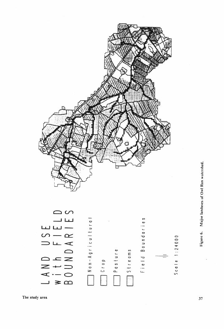
Figure 6. Major landuses of Owl Run watershed. ......... 0... 0 ce eee eee eee eens 37

Figure 7. Regression analysis for runoff simulation (Owl Run watershed 1988) ........ 65

Figure 8. Regression analysis for peak rate stmulation (Owl Run watershed 1988) ....... 66

Figure 9. Regression analysis for sediment yield simulation (Owl Run watershed 1988). .. 67

Figure 10. Regression analysis for total N loading simulation (Qwl Run watershed 1988). . 68

Figure 11. Regression analysis for total P loading simulation (Owl Run watershed 1988). . 69

Figure 12. Regression analysis for runoff simulation (Owl Run watershed 1987) ........ 70

Figure 13. Regression analysis for peak rate simulation (Owl Run watershed 1987) ....... 71

Figure 14. Regression analysis for sediment yield simulation (Owl Run watershed 1987). .. 72

Figure 15. Regression analysis for total N loading simulation (Owl Run watershed 1987). . 73

Figure 16. Regression analysis for total P loading simulation (Owl Run watershed 1987). . 74

Figure 17. Rainfall frequency analysis of Owl Run watershed .................0005- 79

Figure 18. Erosion index (EI) frequency analysis of Owl Run watershed .............. 80

Figure 19. Relationship between rainfall amounts and corresponding EI values ......... 86

Figure 20. Contribution of representative events to annual runoff ................... 90

Figure 21. Contribution of representative events to annual sediment yield ............. 91

List of Illustrations vil

Figure

Figure

Figure

Figure

Figure

Figure

Figure

Figure

Figure

Figure

22.

23.

24.

25.

26.

27.

28.

29.

30.

31.

Contribution of representative events to annual total N loading ............. 92

Contribution of representative events to annual total P loading ............. 93

Distributions of contributions of storm events to annual runoff ............. 94

BMPs currently installed in Owl Run watershed ............0 0000s 97

Critical areas of sediment yield - Pre-BMP - Level A simulation ........... 110

Critical areas of sediment yield - Post-BMP - Level A simulation .......... 111

Critical areas of sediment yield - Pre- BMP - Level B simulation ........... 112

Critical areas of sediment yield - Post-BMP - Level B simulation .......... 113

Critical areas of sediment yield - Pre-BMP - Level C simulation ........... 114

Critical areas of sediment yield - Post-BMP - Level C simulation .......... 115

List of Hlustrations Vili

List of Tables

Table

Table

Table

Table

Table

Table

Table

Table

Table

Table

Table

Table

Table

Table

Table

Table

Table

Table

Bow

oN

DR WN

10.

11.

12.

13.

14.

15.

16.

17.

18.

Summary of widely used NPS pollution models. ............ 0.00. ewes 19

Soil types in the Owl Run watershed. ............ cee eee ee eens 33

Typical Landuses in the Owl Run watershed. ......... 0... 0c ee eee eee 34

Soil and water quality parameters monitored at the Owl Run Watershed ....... 39

. Summary of selected AGNPS parameters used for Owl Run watershed. ........ 46

. Values of selected AGNPS parameters related to landuse in Owl Run watershed. . 47

Summary of Owl Run Simulations for 1988. 2... 0... 0... ee ee eee 57

Summary of Owl Run Simulations for 1987. ......... 0.0.0... ce eee eee eee 58

Summary of statistical analysis for 1988. 2.2... ee eee ene 59

Summary of statistical analysis for 1987. 2.0... 1. ee ee ee ee eee 60

Summary of contributions of representative events to runoff and sediment yield. . 83

Summary of contributions of representative storms to TN, TP, and COD loadings. 85

Comparison of annualized simulations with recorded data from Owl Run watershed. 89

Summary of parameters for no-till simulation. ................--...008- 101

Summary of parameters for stripcropping simulation. .................06. 102

Comparison of simulations before and after the subdivisions of cells for VFS and fencing 6... tt te ee eee eee eee eee tenes 104

Virginia state cost-share rate for major BMPs. ............... 20sec euee 106

Annual pollutant reductions by different BMP scenarios. ................. 107

List of Tables ix

Introduction

Nonpoint source (NPS) pollution, resulting from modern agricultural activities and urban de-

velopments, has been recognized as a significant source of water quality degradation in the United

States. Agricultural nonpoint source pollution, which is diffuse in nature and dominated by natural

processes, is responsible for a significant portion of pollution in large water bodies such as the

Chesapeake Bay [USEPA, 1983]. Main types of agricultural NPS pollution include sediment,

chemical fertilizers, pesticides, and animal wastes.

Soil erosion on nation’s croplands occurs at an average annual rate of about 20 Mg/ha, twice the

acceptable rate considered by some soil conservationists [Dempster and Sterna, 1979]. Soil erosion,

accelerated by human activities on the land, causes numerous sediment-related water quality prob-

lems such as habitat alteration and other adverse effects on aquatic life; filling of water courses and

decreasing of capacities of lakes and reservoirs; increasing the complexity and the cost of treating

water supplies for municipalities and industries; and reducing the recreational value of water bodies.

Many pollutants get absorbed to fine soil particles transported by surface runoff, and deteriorate the

downstream water bodies. In the United States, over 4 billion tons of sediment are delivered into

streams and rivers every year, about half of this amount originates from agricultural lands [Council

on Environmental Quality, 1980}.

Introduction 1

Major NPS pollutants of concern are sediment, nitrogen (N) and phosphorus (P). Fertilizers,

animal wastes, and crop residues are major sources of N and P. Excessive amount of soluble inor-

ganic P and N causes eutrophication in water bodies like the Great Lakes and the Chesapeake Bay.

Eutrophication, which is defined as explosive growth of aquatic plants, particularly algae, causes

increased turbidity; reduced oxygen levels; taste and odor problems; and aesthetically decreases

recreational values of surface waters. Excessive nitrate-N in water supplies can also cause animal

and human health problems [Duttweiler and Nicholson, 1983]. Agricultural and urban runoff may

also carry large amounts of toxic metal , pesticides, and other organic chemicals. These materials

may result in water quality problems in water supplies, commercial and recreational fisheries, and

decreased species in aquatic ecosystem.

To solve the nonpoint source pollution problems mentioned above, various approaches have

been considered by agencies in charge of NPS pollution control. These approaches, intended to

minimize the negative environmental effects of land use activities while maintaining the productivity

of the land, include the use of agricultural best management practices, or BMPs. Important BMPs

which reduce pollutant carriers such as surface runoff and sediment, include conservation tillage,

terraces, contouring, and cover crops. Other BMPs intended to reduce pollutant concentrations

involve the method, rate, timing, and formulation of fertilizers and pesticides. Such BMPs include

integrated pest management and improved fertilizer and animal waste management. There are also

structural BMPs which reduce pollutant delivery such as filter strips, ponds, grassed waterways,

terraces, and contouring.

To put the measures and steps of solving nonpoint source pollution problems into practice, the

effectiveness of the BMPs need to be evaluated first. In general, the most ideal way of evaluating

the impact of management practices on NPS pollution control is the establishment of a compre-

hensive monitoring system. Such systems allow detailed data collection and analysis for the assess-

ment of the effectiveness of BMPs. For most watersheds, however, it is not economical to install

monitoring systems. Watershed models are powerful tools to carry out the task of BMP assessment.

These models, however, need to be validated first to demonstrate their applicability on certain

watersheds. The validation work has rarely been done for most distributed parameter models be-

Introduction 2

cause of the need for excessive amount of field data for such models. The extensive data collected

from the Owl Run watershed, located in Fauquire County, Virginia, makes it possible to validate

distributed NPS models for Virginia’s Piedmont conditions [Mostaghimi, et al., 1989].

Even if a monitoring system is installed in a watershed, it is unlikely that the “critical areas” can

be demonstrated because of the diffuse characteristics of the nonpoint source pollution (nonpoint

sources generally cannot be monitored at their points of origin, and their exact sources are difficult

or impossible to trace). A critical area is defined as the small fraction of a watershed responsible

for a majority amount of sediment and chemical loadings to downstream water bodies. Distributed

parameter watershed models have the capability to identify the critical areas within the watershed.

Therefore, if pollution control activities can be concentrated in these areas, greater water quality

improvements can be expected with limited funds.

Objectives

The overall goal of this study was to investigate the applicability of a NPS pollution model to

small watersheds in Virginia Piedmont areas. The specific objectives were:

a. To perform a critical review of existing distributed watershed models and select a suitable model

for assessing NPS pollution in Virginia Piedmont areas. The model should have the ability to

evaluate the effectiveness of specific BMPs in terms of pollutant reductions.

b. To validate the model by comparing the model predictions with the data collected from a small

agricultural watershed in Virginia.

c. To use an annualization procedure to convert the event-based simulation results of the model

to average annual results so that the BMPs effectiveness can be evaluated on a long-term average

Introduction 3

basis, and compare the annualized simulation results with long-term average annual values of re-

corded data.

d. To identify NPS pollution critical areas on the watershed and propose suitable BMPs for re-

ducing annual pollutant loadings.

Introduction 4

Literature Review

A classification of different models is discussed in this chapter in order to recognize relevant

models by their specific characteristics. Widely accepted and used nonpoint source pollution

models are reviewed and their advantages and limitations are discussed. Based on the review of

models summarized in this chapter, a model is selected for the proposed study.

Classification of Models

To better understand, explain, and describe natural phenomena, variety of models have been

developed to simulate real systems. Different criteria result in different classification of models,

which reflect special interests or needs within a particular field of study. However, any model can

be categorized as either a material or a mathematical model [Haan, 1982]. Material models can

further be classified as either iconic or analog models, which have little to do with the topic of this

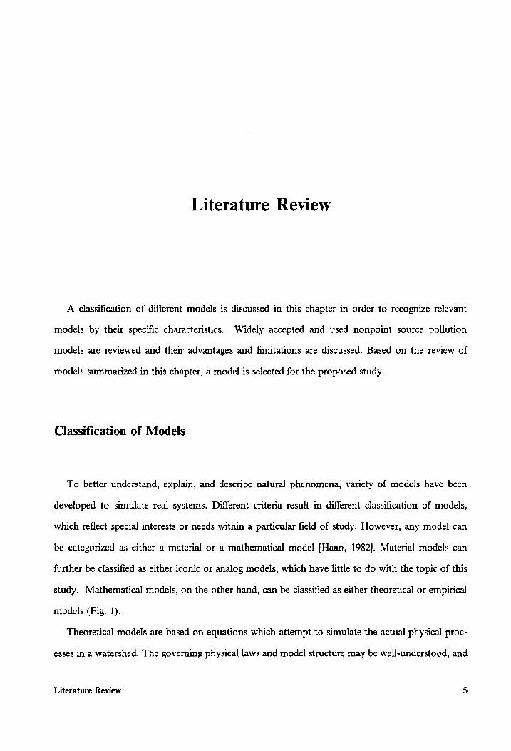
study. Mathematical models, on the other hand, can be classified as either theoretical or empirical

models (Fig. 1).

Theoretical models are based on equations which attempt to simulate the actual physical proc-

esses in a watershed. The governing physical laws and model structure may be well-understood, and

Literature Review 5

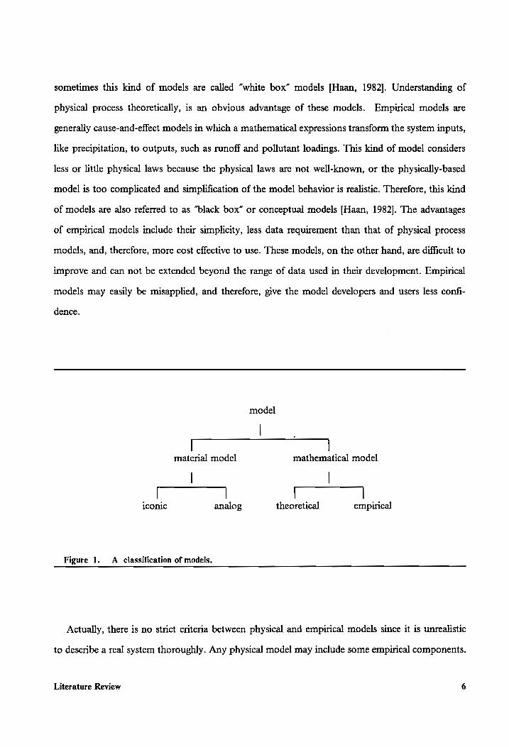
sometimes this kind of models are called “white box” models [Haan, 1982]. Understanding of

physical process theoretically, is an obvious advantage of these models. Empirical models are

generally cause-and-effect models in which a mathematical expressions transform the system inputs,

like precipitation, to outputs, such as runoff and pollutant loadings. This kind of model considers

less or little physical laws because the physical laws are not well-known, or the physically-based

model is too complicated and simplification of the model behavior is realistic. Therefore, this kind

of models are also referred to as “black box” or conceptual models [Haan, 1982]. The advantages

‘of empirical models include their simplicity, less data requirement than that of physical process

models, and, therefore, more cost effective to use. These models, on the other hand, are difficult to

improve and can not be extended beyond the range of data used in their development. Empirical

models may easily be misapplied, and therefore, give the model developers and users less confi-

dence.

model

[ 4 material model mathematical model

| | [ [

iconic analog theoretical empirical

Figure 1. A _ classification of models.

Actually, there is no strict criteria between physical and empirical models since it is unrealistic

to describe a real system thoroughly. Any physical model may include some empirical components.

Literature Review 6

It is clear, however, that the more the physical components are used in a model, the more confi-

dence a modeler or a user will have in its application.

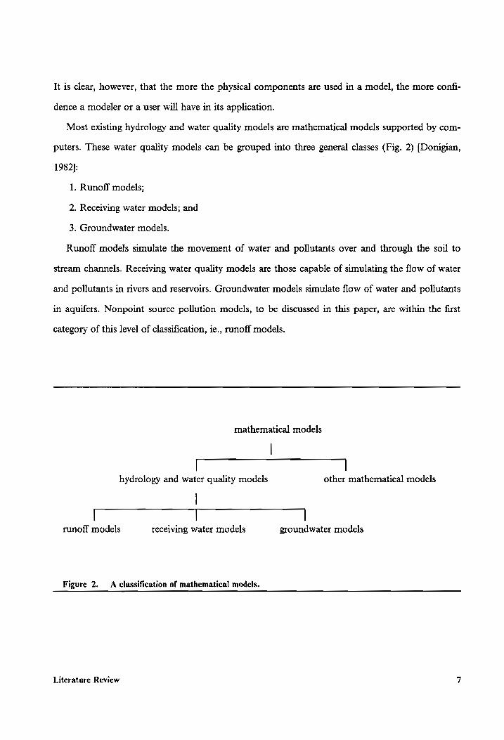
Most existing hydrology and water quality models are mathematical models supported by com-

puters. These water quality models can be grouped into three general classes (Fig. 2) [Donigian,

1982):

1. Runoff models;

2. Receiving water models; and

3. Groundwater models.

Runoff models simulate the movement of water and pollutants over and through the soil to

stream channels. Receiving water quality models are those capable of simulating the flow of water

and pollutants in rivers and reservoirs. Groundwater models simulate flow of water and pollutants

in aquifers. Nonpoint source pollution models, to be discussed in this paper, are within the first

category of this level of classification, ie., ranoff models.

mathematical models

| | |

hydrology and water quality models other mathematical models

| | |

runoff models receiving water models groundwater models

Figure 2. A classification of mathematical models.

Literature Review 7

Three levels of modeling can be identified according to model structure and modeling subject.

1) Individual process models; 2) component models; 3) Integrated watershed models

[Ozgazielinska, 1976]. Individual process models describe one of the physical processes involved in

the hydrologic cycle. Evaporation from free surface of water, flow in vadose zone, and unsteady

surface flow are examples of individual process models. Component models include linked models

of individual processes. These single process models can be run individually or simultaneously.

Examples of component models include: evapotranspiration, direct surface runoff, erosion and

subsurface flow. An integrated watershed model is a comprehensive model that consists of a set of

linked component models and an operator that apportions the flow of water to the individual

components in proper order. Such models are developed by combining components and have a

well-defined structure. Most NPS models are integrated watershed models.

Mathematical hydrology and water quality models can also be classified according to the fol-

lowing criteria:

1. Static and dynamic models

2. Stochastic and deterministic models

3. Lumped and Distributed Parameter Models

4. Screening and hydrologic assessment models

Static models do not use time as an independent variable, i.e. the real system is stimulated under

the assumption of a steady-state condition, while dynamic models are time- dependent [Haan,

1982]. Dynamic models can also be event-based or continuous models. Event-based models at-

tempt to simulate the hydrologic response during a storm event. They can better describe some of

the processes in detail and ignore some processes like evapotranspiration. This kind of models,

however, can not adequately represent long-term processes, and must select design storms to eval-

uate BMPs. Examples of event-based models include ANSWERS [Beaseley and Huggins, 1982],

FESHM [Ross, et al., 1982], and AGNPS [Young, et al., 1985]. Continuous models characterize

long term system response, and they are more appropriate for BMP risk assessment. The models

can account for meteorologic variability. One main disadvantage of continuous models is that they

Literature Review 8

have less details on individual events and some processes of interest may not be adequately de-

scribed for storms. CREAMS [Knisel, 1980], ARM [Donigian and Davis, 1978], HSPF [Johanson

et al., 1981] are examples of continuous NPS models.

A stochastic model considers the chance of occurrence of the variables and introduces the con-

cept of probability into the model. This kind of model requires long term historical data or syn-

thetic records such as precipitation, climatic, runoff, and sediment yield. If all the variables are not

random, or the chance of occurrence is ignored and the model is considered to follow a definite law

of certainty, the model will be a deterministic one [Chow, 1964]. Most of the NPS models are

deterministic.

Lumped models simulate an area under the assumption that all the system’s inputs and the pa-

rameters are uniform. They do not consider spatial variability of topography, soils and surface

cover conditions. Therefore critical areas can not be identified by using this kind of models. Dis-

tributed parameter models, on the other hand, delineate a watershed into fine cells within which soil

properties, crop conditions, and other characteristics of each element are considered to be homo-

geneous. The overall watershed response is obtained by integrating all the elemental responses.

These elements are also influenced by inflows from and outflows to neighboring elements. Obvi-

ously, the computational effort required to use this kind of models is greater than those of lumped

ones. But the models which consider spatial variability make it possible to delineate critical areas.

The additional computation time is compensated by improved accuracy of simulation results.

Screening, or planning models, are useful for identifying problem areas within large basins and

to make preliminary quantitative assessment of BMPs [Novotny, 1986]. Screening models are rela-

tively simple and their predictions are accurate only within an order of magnitude [Novotny, 1986].

Universal Soil Loss Equations (USLE) [Wischmeier and Smith, 1978], and GAMES [Cook, et al.,

1985; Madramootoo, et al., 1988] are examples of screening models. Hydrologic assessment models

are much more complex and can be used to evaluate various conditions or alternative management

scenarios. Hydrologic assessment models can also be subdivided into field-scale and watershed-scale

Literature Review 9

models. Field-scale models are usually lumped models describing hydrologic processes within a field

with uniform soils, crops, topography and weather condition. CREAMS [Knisel, 1980]; GLEAMS

[Leonard, et at., 1987]; and NTRM [Shaffer, et al., 1983] are examples of field scale models.

Watershed-scale hydrologic assessment models have a broad range of capabilities. Some of these

models are event oriented while others are continuous simulation models. Distributed models have

the ability to identify critical sources of NPS pollution in watersheds, and most of them can be

used to simulate effectiveness of various BMP implementatios. Examples of watershed-scale

hydrologic models include AGNPS [Young, et al., 1982]; ARM [Donigian and Davis, 1978]; AN-

SWERS [Beasely and Huggins, 1982]; and BASIN [Heatwole, et al., 1987].

Description of NPS models

WEPP

The USDA Water Erosion Prediction Project model (WEPP) was developed to generate new

water erosion prediction technology for use in soil and water conservation, and environmental

planning and assessment [Gilley, et al. 1988]. The WEPP model 1s a field size model for applying

to areas as large as a few hundred hectares in size. A watershed version is under development which

includes concentrated flow channels. The watershed version of the WEPP is a distributed model

based on a descretization of the study area.

The main advantage of WEPP model is that it uses simple inputs which are commonly available

and understood by personnel in local field offices. The model can also calculate sheet and rill ero-

sion, ephemeral gully erosion, and accounts for effects of climate, soils, topography, and cropping

management conditions on erosion and sediment transport. Furthermore, the model is easy to use

and applicable to a broad range of conditions. The current version of the model does not have a

Literature Review 10

chemical component. WEPP model has not been widely used or tested and verification is needed

before application on a particular field. The model is in its final stages of development.

CREAMS

The CREAMS model (Chemicals Runoff and Erosion from Agricultural Management Systems)

was developed by Agricultural Research Service for agricultural nonpoint source pollution control

research and planning purposes [Knisel, 1980]. With respect to nonpoint sources of pollution, this

model was developed specifically to simulate the response of field size areas. CREAMS is a com-

prehensive model for simulating long term average annual yields from a field. The model considers

infiltration, snow melt, evapotranspiration, plant growth, sediment detachment and transport, nu-

trient and pesticides transport, and even leaching past the root zone [Knisel, 1980]. The model has

two hydrology options: One option uses SCS runoff method, the other is an infiltration-based

runoff component model. CREAMS has also a channel erosion and deposition component and

can be used to evaluate alternative landuse practices and conservation measures [Decoursey, 1985].

The model employs concepts and algorithms representing natural processes, and most of the input

parameters have a physical basis [Heatwole, Campbell, and Bottcher, 1987].

CREAMS has been verified with the data from many regions of the country, and has been

widely used and distributed both nationally and internationally [Knisel and Svetlosanov, 1982]. The

modified version of the model, CREAMS-WT, was developed to better represent the hydrology

of flat, sandy, high-water-table fields [Heatwole et al., 1987]. Data from watersheds in South Florida

flatwood regions were used for model development and verification. The model should also be ap-

plicable to Atlantic and Gulf Coastal Plain areas that have similar hydrologic conditions.

The application of CREAMS is limited to field size areas since it is a lumped parameter model

and does not have the ability to consider spatial variability on a watershed scale. Therefore the

model can not identify critical areas with a watershed.

HSPF

The Hydrologic Simulation Program Fortran (HSPF) is a continuous general model which was

developed by Hydrocomp for the U.S. Environmental Protection Agency [Johanson et al., 1981;

Literature Review It

Decoursey, 1985]. It is a modification of the Stanford Watershed Model-4 [Ccrawford and Linsley,

1966]. This general-purpose model simulates hydrology, sediment, pH, dissolved oxygen, organic

matter, temperature, nutrients, pesticides, salts, bacteria and plankton from land surface entirely

through a channel and reservoir system, including groundwater. HSPF consists of a set of modules

arranged in a hierarchical structure which continuously simulates a comprehensive range of

hydrologic and water quality processes.

HSPF was applied to a watershed in Iowa by Donigian et al. [1983] to predict water quality re-

sulting from agricultural nonpoint sources. Their experiences with the model showed that HSPF

provides a viable and flexible means of estimating the impacts of a wide range of BMPs.

Calibration of HSPF was a hard job, and problems with field-to-stream delivery were also

mentioned by the authors. Formal training is recommended when necessary for those who attempt

to use HSPF because of its complexity [Crowder, 1987]. The biggest drawback of the model is the

empirical base of the many of its hydrologic parameters. Several years of recorded data are needed

to obtain reliable input values for many of these parameters. Large amount of human efforts needed

for application of the model is associated with data management and calibration of the parameter

values. HSPF is a lumped model and can not be used to identify problem areas within a watershed.

FESHM

An event-oriented, distributed parameter hydrologic model, Finite Element Storm Hydrograph

Model (FESHM), was developed and modified for simulating runoff in ungaged areas and for as-

sisting in nonpoint source pollution control planning [Ross, 1978; Ross, Wolfe, et al., 1982]. The

model has the ability to identify critically eroding areas within a watershed.

FESHM has two components: hydrology and sedimentation. Current version of the model does

not have a nutrient or pesticide component. It divides the watershed into flow elements and the

geographic information characteristics are lumped within each element. The finite element structure

allows the model to route rainfall excess and sediment yield downstream. The governing flow

equations of continuity and momentum were solved by the finite element numerical technique.


In subdividing a watershed, FESHM uses a procedure with two levels of discretization.

Hydrologic Response Units (HRU’s) are defined in determining rainfall excess, which are based on

overlay of soil mapping units and land use maps. Elements used to route overland flow are defined

based on the drainage and topographic characteristics of the watershed. The HRU’s rainfall excess

quantities are area-weighted within each flow element. This approach gives the model sufficient

flexibility to alter the number and position of overland flow elements to reflect wide spatial vari-

ations in rainfall excess generation.

Alternative land management practices can be simulated in terms of runoff and sediment loss

by using FESHM. The model simulates the management practices by changing the soil and cover

condition parameters in the input data file. Sediment in streams, nutrient, and pesticide components

are not available in the current version.

Difficulties were found in simulating low rainfall and low runoff events [Smith and Hebbert,

1979; Keith Beven, 1985]. This disadvantage of the model was ascribed to the lack of allowing

runoff generated on a relatively impervious unit to reinfiltrate on other units downslope. The

sediment transport component of the model has not been verified extensively. The sensitivity

analysis of the model to input parameters was carried out by Shanholtz et al. [1981]. It was found

that the model is most sensitive to the storage parameter in Holtan’s infiltration equation and hy-

draulic roughness coefficients [Shanholtz, et al., 1981].

ANSWERS

Areal Nonpoint Source Watershed Environment Response Simulator (ANSWERS) is another

distributed parameter, deterministic watershed model, which was developed originally by Purdue

University for the EPA Great Lakes Program [Beasley, 1977]. The original version of the model

predicts runoff and sediment loadings but not nutrients. A phosphorus transport component was

incorporated into ANSWERS, and data from rainfall simulator plots were used to verify the model

[Storm, 1987]. The phosphorus transport version of the model was used by Storm et. al. [1988]

to demonstrate BMPs effects on increasing cost-effectiveness of cost-share funds for water quality


improvement in the Nomini Creek watershed. ANSWERS divides watershed into a grid of small

square cells. Infiltration, surface retention, soil moisture, sediment detachment and transport, and

nutrient losses are calculated for each cell. These cellular responses are routed to cells downslope

and finally to the watershed outlet.

ANSWERS can be used as a planning tool for quantitatively evaluating the benefits of various

BMP scenarios for nonpoint source pollution control and even structural BMPs such as ponds,

grass waterways, and parallel tile-outlet terraces [Beasley and Huggins, 1982]. Like other distributed

watershed models, with its erosion submodel, ANSWERS can identify critical areas within a

watershed. Another advantage of the model is that the hydrology component uses break-point

rainfall data and deterministic equations to estimate infiltration, surface retention and detention, and

percolation to predict rainfall excess.

One of the disadvantages of the ANSWERS model is that it does not consider channel erosion.

It allows sediment degradation in channels only at the previously deposited areas. This limitation

of the model would be a problem if channel erosion occurs significantly in watersheds. Like other

distributed parameter watershed models, ANSWERS needs large amount of input data to describe

the conditions within each element of the watershed. Since each element is like a lumped parameter

watershed and requires about the same computation time as a lumped model does, the computer

time needed for a distributed model is much greater than that of a lumped model. With the devel-

opment of digital remote sensing techniques and other computerized inventory survey, this time

consuming work, however, is being reduced considerably [Feezor et al. 1989}.

AGNPS

Two Agricultural Nonpoint Source Pollution Models, AGNPS-I for areas from 500 to 25,000

acres and AGNPS-II for areas from 2.5 to 500 acres were developed in Minnesota [Young, et al.,

1985]. Both of the models simulate runoff volume and peak rate, sediment detachment and trans-

port, and nutrient and oxygen concentrations for single storm events.


AGNPS is a distributed parameter, event-based model. Hydrology, erosion, sediment transport,

nitrogen, phosphorus and chemical oxygen demand transport are calculated for each cell. AGNPS

can also consider point sources such as sediment from gullies, water, sediment, nutrient and

chemical oxygen demand (COD) from animal feedlots, springs, and other point sources. Although

AGNPS uses a cellular database like ANSWERS, the relationships used in each component cal-

culation is much simpler than those used in ANSWERS such that AGNPS requires much less

computational effort. Because of its simplicity, a PC version of AGNPS was developed by Young

et al. [1985] to simulate watersheds with areas from 2.5 to 8,000 acres.

An apparent advantage of the model is that it can treat nutrient contributions from animal

feedlots as point sources and route them with contributions from diffuse sources. Streambank,

streambed, and gully erosion are also accounted for using estimated values as point sources.

Sediment from these sources is added to upland sediment and considered in the transport phase of

the model.

The main difficulty in using AGNPS is that the preparation of input data file is very time con-

suming. The total time required to collect input data for the model and enter the data into files re-

quires 20 minutes per cell [Young, et al. 1987, Koelliker and Humbert, 1989]. Efforts were made

by some researchers to develop software for interfacing geographic information systems with the

AGNPS input data files [Hirschi, 1989].

The model has been tested for runoff estimations with data from 20 watersheds in the north

central United States. Sediment yield estimates of the model with data from three watersheds in

Iowa and Nebraska compared favorably with the measured values from the three watersheds

[Young, et al., 1989]. The chemical component of AGNPS has not been tested on watershed scale

because of lack of field data from watersheds. An annualization routine was also developed to

evaluate long-term effects of BMPs on reducing pollution from nonpoint sources [Koelliker and

Humbert, 1989].

SWRRB


The SWRRB model (Simulator for Water Resources in Rural Basins) was developed from

CREAMS to predict the effect of management decisions on water and sediment yields within larger

and more complex basins [Arnold, 1987].

The model was tested on more than ten large watersheds from eight Agricultural Research Ser-

vice (ARS) locations throughout the United States. The results showed that SWRRB can be used

to simulate water and sediment yields under a wide range of climatic conditions, soil properties,

topography, landuse, and management practices [Arnold, 1987].

Recent improvements to the model include: 1). addition of a return flow component; 2). the

incorporation of a component evaluating the effects of ponds and other reservoirs on water yield;

3). the addition of a weather model for long term simulation including rainfall, solar radiation and

temperature; 4). the development of a different method to predict peak runoff rate; and 5). the

addition of a simple flood routing component [Amold, 1987].

The model is based on daily rainfall hydrology so it does not have the ability to model event-

based storms. SWRRB does not have a chemical component to simulate transport of nutrients and

pesticides. A recent study showed that the SWRRB and AGNPS obtained much better simulation

results than CREAMS, EPIC, and ANSWERS. The data used were collected from several

watersheds in Mississippi [Bingner, et al., 1989].

The model was expanded to allow simultaneous computations on several subbasins. The largest

number of subbasins in the simulation by Arnold [1987] was five. It is unlikely that the model can

be classified as a distributed parameter model. Thus the model does not have the ability to identify

critical areas within a watershed.

GAMES

The Guelph model for evaluating effects of Agricultural Management Systems on Erosion and

Sedimentation (GAMES) is an event-based model which was developed at the University of

Guelph [Cook et al, 1985, Rudra et al, 1986, and Madramootoo et al., 1988]. GAMES is a dis-

tributed parameter model but its hydrologic response units are not elemental squares like that of


ANSWERS and AGNPS, these cells are irregular-shaped, which are delineated by natural and

man-made boundaries such as soils, topography, and land use.

' The principal inputs to the model are the rainfall erosion index (EJ) and variables describing the

soils, crops, and physical characteristics of each cell. The principal outputs from the model on a

cellular level are gross erosion, sediment yield to the adjacent cells and sediment yield to the chan-

nel, total gross erosion, average erosion, and total sediment yield. No nutrient and pesticide com-

ponents are available in the current version of the model. Since GAMES is simply a modification

of a seasonal erosion and sediment yield model, no hydrologic output is available.

ARM

Agricultural Runoff Management (ARM) model [Donigian and Davis, 1978; Davis and

Donigian, 1979] is a lumped parameter, continuous simulation model. ARM simulates runoff,

sediment, phosphorus, nitrogen, and pesticide loadings to surface waters from both surface and

subsurface sources. The hydrologic component of the model is an overland flow version of the

Stanford Watershed Model [Ross, 1970], which simulates small watersheds from 200 to 500 ha in

size.

The main advantage of ARM model is its comprehensiveness. It estimates runoff, sediment,

nutrient (N and P) and pesticides. The model has many drawbacks of lumped models, therefore the

model has to assume uniform landuse, cropping management practices, soils, and topography.

Furthermore, ARM is not suitable for modeling ungaged watersheds because it needs historical

records of runoff and water quality for calibration. ARM model does not consider channel erosion.

Crowder (1987) reported that calibration of ARM is necessary for each application of the model.

The author concluded that the model simulated monthly phosphorus loadings to runoff satisfac-

torily.

EPIC


Erosion Productivity Impact Calculator (EPIC) was developed by Williams et al. [1982] to de-

termine the relationship between soil erosion and crop productivity. EPIC is a continuous model

which simulates annual and perennial crop growth by predicting long term effects of soil erosion

on crop production. The model simulates, on a daily basis, hydrologic condition, sediment loss,

soil nutrient properties, soil temperature, effect of tillage, plant growth stage, and daily weather, if

the daily data are not available.

The multi-year simulation capability of the EPIC model is its main advantage. Jt is able to run

eleven different crops in a crop rotation schedule. Detailed description of the recent version of the

model was given by Williams et al. [1988]. Validation work was done for crop yield and runoff

components [Williams and Renard, 1985]. The model has been used to determine the impact of soil

erosion for the 1985 Resource Conservation Act appraisal [Putman et al., 1988]. EPIC is a field

size, lumped parameter model and does not simulate storm event effects. The model can not be

applied to a watershed for identifying critical areas.

Summary

A distributed parameter, comprehensive watershed model is needed to investigate the impact

of BMPs on surface water quality from Owl Run watershed. This watershed was selected for

monitoring because of its topography, landuse, and soils, which are typical characteristics of

watersheds in the northern part of Virginia. A monitoring system was installed in the watershed in

1986 and a substantial amount of water quality, quantity and landuse data necessary to validate the


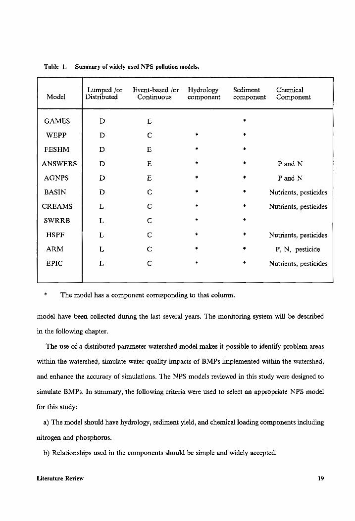
Table 1. Summary of widely used NPS pollution models.

Lumped /or _Event-based /or Hydrology Sediment Chemical Model Distributed Continuous component component Component

GAMES D E *

WEPP D C * *

FESHM D E * *

ANSWERS D E * * P and N

AGNPS D E * * P and N

BASIN D C * * Nutrients, pesticides

CREAMS L C * * Nutrients, pesticides

SWRRB L C * *

HSPF L Cc * * Nutrients, pesticides

ARM L Cc * + P, N, pesticide

EPIC L C * * Nutrients, pesticides

* The model has a component corresponding to that column.

model have been collected during the last several years. The monitoring system will be described

in the following chapter.

The use of a distributed parameter watershed model makes it possible to identify problem areas

within the watershed, simulate water quality impacts of BMPs implemented within the watershed,

and enhance the accuracy of simulations. The NPS models reviewed in this study were designed to

simulate BMPs. In summary, the following criteria were used to select an appropriate NPS model

for this study:

a) The model should have hydrology, sediment yield, and chemical loading components including

nitrogen and phosphorus.

b) Relationships used in the components should be simple and widely accepted.


c) The model should have the ability to simulate different kinds of BMPs.

d) The model should be a distributed one to enable the identification of critical areas and simulate

various BMPs implemented at different locations within the watershed.

e) Event-based models are preferred for this study since a comprehensive database exists for storm

events on Owl Run watershed.

Table 1 gives a summary of selected NPS models and their major characteristics. As indicated

in the table, the first six models are distributed parameter models, of which BASIN, ANSWERS,

and AGNPS have all the necessary components mentioned in the above criteria, and all of them

have the ability to simulated various BMPs, in addition, ANSWERS and AGNPS are event-based

models.

Three years of comprehensive data was available from Owl Run watershed, including rainfall

amount, runoff volume, sediment yield, total nitrogen and total phosphorus loadings for individual

events. Therefore, it was thought that an event based model should be selected, and validated by

using data from these storm events.

ANSWERS and AGNPS are believed to be the most applicable NPS models to our situation

based on the review of the models and data available. AGNPS was selected for this study because

of its widely accepted, simple relationships, user-friendly graphics functions, and

comprehensiveness. AGNPS has been successfully tested for various conditions throughout the

U.S. and more efforts are being made to interface the model with Geographic Information System

(GIS) to allow more convenient applications. A detailed description of AGNPS is included in the

next chapter.


The Agricultural Nonpoint Source Pollution Model

(AGNPS)

Introduction

The event-based, distributed parameter model AGNPS simulates runoff volume, peak flow rate,

sediment, and nutrient transport from agricultural watersheds. The nutrients considered include

nitrogen (N) and phosphorus (P). Basic model components include hydrology, erosion, sediment,

and chemical transport. The model also considers point sources of sediment, water sources, nutri-

ents and chemical oxygen demand (COD) from animal feedlots, springs, and other point sources

[Young, et al. 1989]. Sediment and chemicals from these sources are added to upland sediment and

chemicals considered in the transport phase of the model. Water impoundments are also considered

as areas of sediment deposition and adsorbed nutrients. AGNPS divides a watershed into uniform

square areas and analysis can be made at any point within the watershed.

Koelliker and Humbert [1989] used the PC version (2.5) of AGNPS on five watersheds in

northeast Kansas. An annualization routine was developed in the study to estimate average annual

results rather than single event results for water quality planning purposes. The study confirmed

the promising use of the AGNPS model to develop predictions for relative changes in yields as a

The Agricultural Nonpoint Source Pollution Model (AGNPS) 21

result of specific changes in watershed conditions. There was not adequate data available to validate

or calibrate the model. The study was based on a sedimentation survey of small reservoirs in Kansas

for the year 1960 [Holland, 1971]. The predicted sediment and water yields agreed reasonably good

with the measured data.

Several NPS models including AGNPS were used to simulate runoff and sediment yields from

three watersheds in Mississippi [Bingner, et al., 1989]. In this study, the AGNPS model was modi-

fied to simulate system response continuously holding all of the parameters constant for a given

year, except for rainfall, EI value and C factor used in the USLE. Simulated values by AGNPS

were compared with measured values from a number of storm events, over several years, on each

watershed. The comparison showed that no model worked very well for every situation of runoff

and sediment yield on the watersheds. Results produced by AGNPS, however, were close to the

measured values in many situations.

The AGNPS model was tested for runoff evaluations on 20 different watersheds in north central

United States by Young, et al.[1989]. A regression analysis of the estimated peak runoff values on

the observed values yielded a slope of 0.984, a good agreement between estimated and observed

values. Testing for sediment yield estimates were carried out on three watersheds, with two of them

being in Iowa, the other in Nebraska [Young, et al., 1989]. The estimation from the model com-

pared favorably with the measured values from the three watersheds.

Data from seven different watershed in Minnesota collected over a 3-year period were used to

test the chemical components of the AGNPS model [Young, et al., 1989]. The comparison of

measured versus estimated N and P concentrations from 20 different sampling points in the seven

watershed indicated that AGNPS provided realistic predictions of nutrients concentrations in runoff

water. Major applications following the testing of the model were accomplished on two large

watersheds in Minnesota [Young, et al., 1989] to identify critical areas within the watersheds, and

evaluate BMP effectiveness.

As mentioned previously, data file preparation for AGNPS is a time consuming work. Young’s

estimate [1987] was 20 minutes per cell to collect necessary data and enter the data into the files.

Researchers have tried to link Geographic Information Systems (GIS) to AGNPS model to save


the laborious time [Feezor, et al., 1989; Needham and Baxter, 1989]. The interfacing GIS with

AGNPS model can greatly enhance the efficiency of the model capabilities. In Feezor’s study

[1989], statistical evaluation of grid size comparison demonstrated that a user should use the

smallest grid size available to obtain certain degree of accuracy. High level automation of data

conversion is still expected to allow quick evaluation of alternative management practices.

The four components of the model, hydrology, soil erosion and sediment transport, chemical

transport, and point sources are described in detail in the following sections.

Hydrology

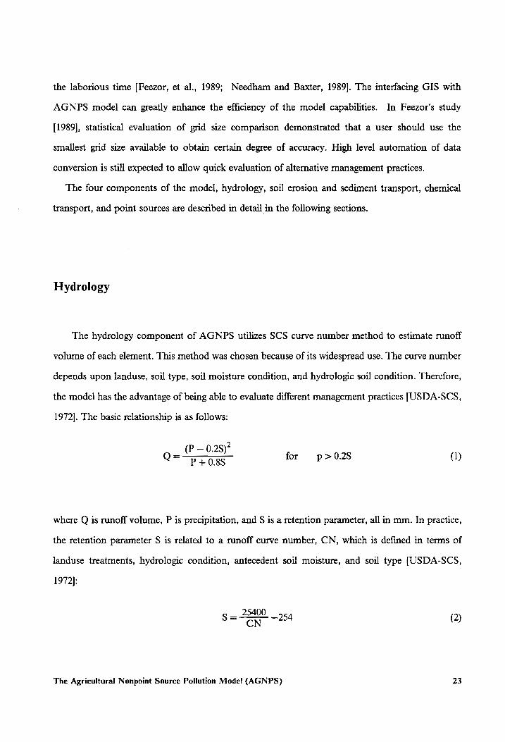
The hydrology component of AGNPS utilizes SCS curve number method to estimate runoff

volume of each element. This method was chosen because of its widespread use. The curve number

depends upon landuse, soil type, soil moisture condition, and hydrologic soil condition. Therefore,

the model has the advantage of being able to evaluate different management practices [USDA-SCS,

1972]. The basic relationship is as follows:

_ (P= 0.28)" Q= P+0.8S for p> 0.28 (1)

where Q is runoff volume, P is precipitation, and S is a retention parameter, all in mm. In practice,

the retention parameter S is related to a runoff curve number, CN, which is defined in terms of

landuse treatments, hydrologic condition, antecedent soil moisture, and soil type [USDA-SCS,

1972]:

_ 25400 _ 564 S CN (2)


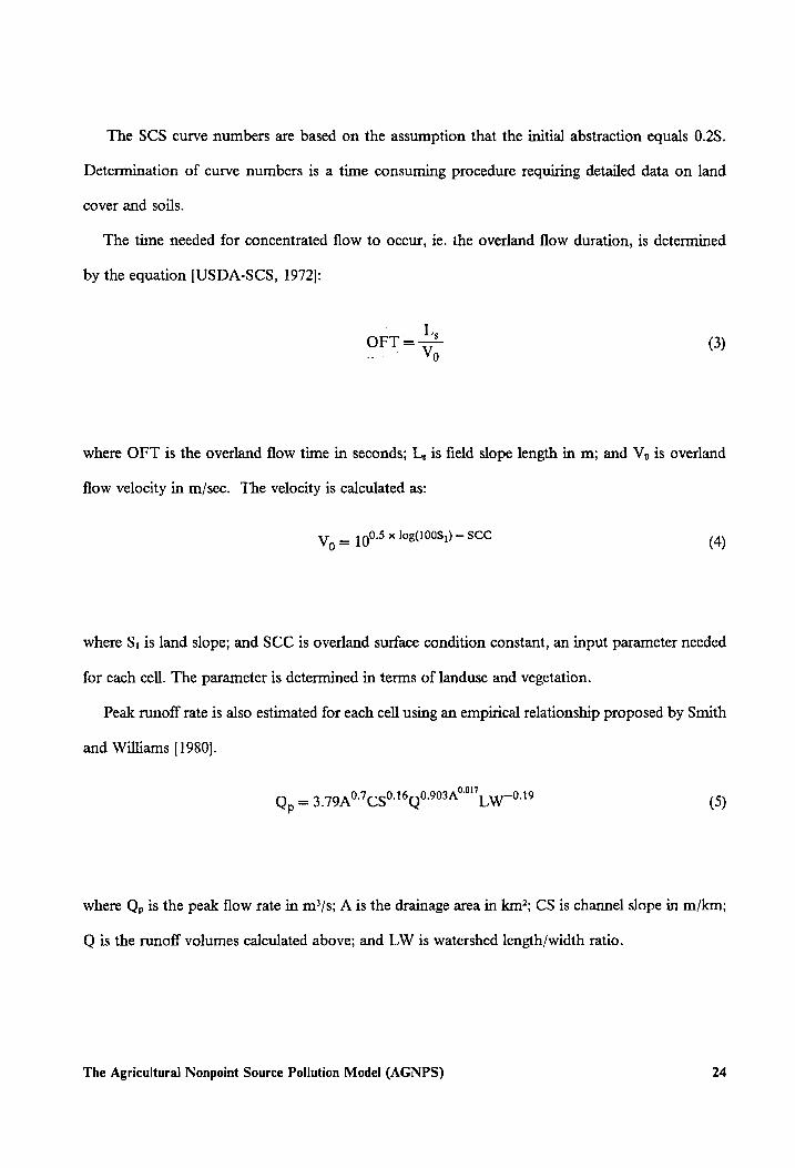
The SCS curve numbers are based on the assumption that the initial abstraction equals 0.2S.

Determination of curve numbers is a time consuming procedure requiring detailed data on land

cover and soils.

The time needed for concentrated flow to occur, ie. the overland flow duration, is determined

by the equation [USDA-SCS, 1972]:

L, OFT = Vv, (3)

where OFT is the overland flow time in seconds; L, is field slope length in m; and Vp» is overland

flow velocity in m/sec. The velocity is calculated as:

Vo = 1005 * 108(1008)) ~ SCC (4)

where S, is land slope; and SCC is overland surface condition constant, an input parameter needed

for each cell. The parameter is determined in terms of landuse and vegetation.

Peak runoff rate is also estimated for each cell using an empirical relationship proposed by Smith

and Williams [1980].

017 0 Q, = 3.79 A2-7 50-16 0-903A07 70.19 (5)

where Q, is the peak flow rate in m/s; A is the drainage area in km’; CS is channel slope in m/km;

Q is the runoff volumes calculated above; and LW is watershed length/width ratio.


Erosion and Sediment Transport

The erosion and sediment transport component of AGNPS uses a modified form of the Uni-

versal Soil Loss Equation to estimate upland erosion for single storm events [Wischmeier, et al.

1978].

The USLE equation used in AGNPS is:

SL = (EI)KLSCP(SSF) (6)

where SL is soil loss; EI is the energy index, which is the product of the total storm kinetic energy

and maximum 30-minute intensity; K is soil erodibility factor; LS is topographic factor representing

slope length and steepness; C is the crop and management factor; P is the supporting practice factor;

and SSF is a factor to adjust for slope shape within each cell. All these factors are defined and cal-

culated using procedures in USDA Agricultural Handbook 537 [Wischmeier and Smith, 1978].

Eroded soil are divided into five particle size classes -- clay, silt, small aggregates, large aggregates,

and sand.

The detached sediment is routed from cell to cell throughout the watershed to the outlet after

calculation of runoff and upland erosion. The method used for sediment routing involves equations

for sediment transport and deposition described by Foster et al. [1981] and Lane [1982]. The basic

routing equation, derived from the steady-state continuity equation is as follows:

Q,(x) = Q,(0) + Q.1(x/L,) — j D(x)Wdx (7)

where Q,(x) is the sediment discharge at downstream end of channel reach; Q,(0) is the sediment

discharge at upstream end of the channel reach; Q,, is lateral sediment inflow; x is downslope dis-


tance; L, is the reach length; D(x) is sediment deposition rate at point x; and W is the channel

width. The sediment deposition rate is estimated as:

D(x) = LV,,/a(x) ILq,(x) — 2,(x)] (8)

where V;,; is particle fall velocity; q(x) is the discharge per unit width; q,(x) is sediment discharge

per unit width; and g,(x) is the effective transport capacity per unit width. The effective transport

capacity, g,, 1s computed using a modification of the Bagnold stream power equation [Bagnold,

1966], as follows:

2

g,(x) = fk 7 (9)

where f is an effective transport factor; k is transport capacity factor; t is sheer stress determined

by types of soil texture; and V is the average channel flow velocity determined by the Manning’s

equation. Sediment load for each of the five particle sizes is calculated using:

Vis

q(0)

Vss85(X) [q,(0) —~ g,(0)] ™ q(x) J] (10)

2q(x) 2q(x) + OxV.,

Q.0) = TQ) +Q1 FE --GEL

where Q,(x) is the particle discharge at the cell outlet and other symbols are as defined previously.

This is the basic routing equation used in the sediment transport model.

Chemical Transport

The chemical component of the model estimates N, P, and COD transport throughout the

watershed, using the procedures adapted from CREAMS [Frere, et al, 1980] and a feedlot evalu-


ation model [Young, et al., 1982]. It calculates soluble and sediment-bound phases separately. Nu-

trient yield in the adsorbed phase is calculated using total sediment yield from a cell:

Nut,og = (Nut, x Q,(x) x ER (11)

where Nutseg is N or P transported by sediment; Nut; is N or P content in the soil; and ER is

enrichment ratio calculated as:

ER = 7.4x Q,(x)°? x T; (12)

where Q,(x) is the sediment yield and T; is an adjustment factor for different soil textures. The val-

ues for clay, silt, sand, and peat are 1.15, 1.00, 0.85, and 1.50 respectively [Young, et al., 1987; 1985].

Considering the effects of nutrient levels on rainfall, fertilization, and leaching, the soluble nu-

trients contained in runoff are estimated as follows:

Nut) = CayrNute,,Q (13)

where Nut,.) is the concentration of soluble N or P in the runoff; Cru is mean concentration of

soluble N or P at the soil surface during runoff; Nute, is an extraction coefficient of N and P

moving into runoff [Frere, et al. 1980]; Q is the total runoff volume.

The COD considered in the model is assumed soluble and the soluble COD is assumed to ac-

cumulate without losses. Computation of COD values in runoff are based on runoff volumes ob-

tained in the hydrology component and average concentration of COD in runoff is available in the

literature [Young, et al., 1985], which is used as the basis for predicting COD concentration for each

cell.


Point Source Inputs

Nutrient and COD concentrations contributed by animal feedlots are treated as point sources

by the chemical component of the model. Contributions from point sources are then routed with

contributions from nonpoint sources.

Chemical contributions from feedlots are estimated with a feedlot pollution evaluation system

developed by Young et al. [1982]. The system divides an animal feedlot into three conceptual areas.

Area | is the animal lot itself, area 2 is the drainage area upstream of the feedlot, and area 3 is the

area from which runoff bypasses the feedlot (area 1) and joins the runoff from the feedlot at its

outlet. The runoff from area 3 dilutes the concentrations of the pollutants in the runoff from the

feedlot area. A buffer area is also defined, within area 3, as the area between the feedlot and its

downstream waterbody. Inputs required by the model include the areas and curve numbers of the

three areas, the surface condition constant, slope and flow length of the buffer area, and the number

and type of animals in the feedlot. The system calculates the concentration and mass of nitrogen,

phosphorus, and COD in the runoff, taking into account the dilution by the tributary water and

attenuation through the buffer area.

Springs, waste water treatment plant discharges, and other point source inputs are accounted for

by entering inflow rates and chemical concentrations to the cells where the point sources are lo-

cated. Sediment from streambank, streambed, and gully erosion is calculated using estimated values

as point sources and is added to the upland sediment. Sediment and runoff routing through

impoundments are carried out using relations described by Laflen et al. [1978]. These relations were

developed for impoundment terraces with pipe outlets. Impoundments reduce peak discharge rate,

total volume of runoff, sediment yield, and chemical loadings.


Owl Run watershed

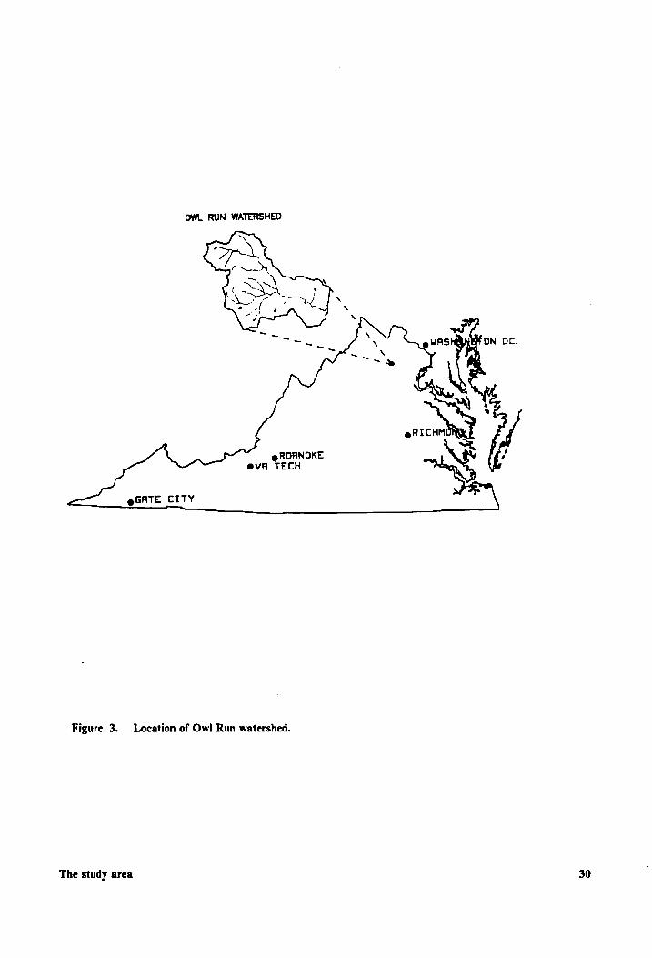
The Owl Run watershed, 1153 hectares in size, is located in Fauquier county, Virginia. The

watershed is 8 km south of Warrenton, Virginia, and 65 km from Washington, D.C. (Figure 3).

The Owl Run watershed was selected to be monitored, as part of the Chesapeake Bay program to

evaluate the impact of animal waste BMPs on downstream water quality. The Owl Run watershed

was chosen because of its high concentration of dairies and lack of animal waste management

practices [Mostaghimi, et al., 1989]. The Owl Run Watershed/Water Quality Monitoring project

was initiated in April 1986 to provide comprehensive assessment of the water quality as influenced

by changes in landuse, agronomic and cultural practices in the watershed over a 10-year study pe-

riod [Mostaghimi, et al., 1989]. Meteorological, hydrologic, biological, soil and water quality, and

landuse information are being monitored at several sites within the watershed. A database man-

agement system for storage and retrieval of hydrologic and water quality information has also been

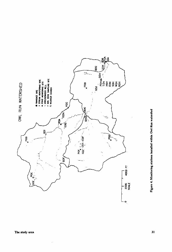
established. The installation of the monitoring system makes it possible to evaluate the effectiveness

of animal waste BMPs on improving the quality of water from the watershed. Figure 3 and figure

4 show the location of the watershed and the monitoring stations installed within the watershed.

Owl Run watershed 29

OWL RUN WATERSHED

@ ROANOKE @VA TECH an

eGATE CITY

Figure 3.

The study area

ae

Location of Owl Run watershed.

30

P2yssazVM UNY

IMC UIYWA

payyersul sues

Burs UOJ]

*p 91NB14

JWOS

44 000%

0002 Lg

1

~~ 409-109

109 |

e

‘ JjOd

NOUVIS WaHiVaM

4aUS ONNdNYS

3409 WOS

» T1aM

YBLWMONNOYD

< 3US

SNISQUNOW ONOd

w 4US

ONRIQUNOW WANS

o AUS

3DVONNY @

Q4HSY3LVM

NAY IMO

31 The study area

Topography: Fauquier county is located in the Piedmount physiographic provinces. The

Piedmount Plateau consists of 80% of the county. The Blue Ridge province in the northwestern

part of the county includes the Blue Ridge Mountains and outlying foothills.

The terrain of the area is predominantly steep and rugged with large rocks strewing over and

protruding from most of the mountain slope. Between the foothills are relatively narrow, rolling

to hilly uplands, which are underlaid by granite rocks. Elevation of the mountains range from 275

m to 725 m above sea level. The valleys are of considerably lower elevation. Main rivers in the

watershed are Rappahannock River, Goose Creek, and their tributaries originated in the Blue Ridge

and its foothills. The northern and eastern parts of the Fauquier County are drained by parts of the

Potomac River drainage system [USDA-SCS and VPI, 1956].

Climate: The climate of Fauquier county, Virginia, is of the humid continental type, with an

average annual rainfall of about 104 cm. It is rather humid and hot in summer with highest tem-

peratures around 32 °C to 35 °C. The extreme temperatures in winters are about -9 °C to -6 °C

which are vigorous but not too severe. A typical characteristic of the winters is frequent cold spells

of short duration. The average frost-free period is 189 days, expending from mid-April to late Oc-

tober [USDA-SCS and VPI, 1956].

Although large amount of rain occurs in spring and summer during the crop growing season, the

distribution of the average annual rainfall in the county is fairly even throughout the year. Runoff

is usually large during summer because of the rainfall intensity. Most of the well-drained upland

soils in the area may actually absorb less moisture during summer season. Heavy thunderstorms

and showers are frequent in summer, late spring, and early fall. Slowly drizzling rains and snow are

main forms of winter precipitation. The wind velocity is greatest in the spring and the average over

the year is 9.7 km/hr.

Soils: The soils on the watershed are mainly shallow silt loams, with Triassic shale being under-

neath. In some areas of the watershed the shale layer is exposed. Areas with high erosion rate are


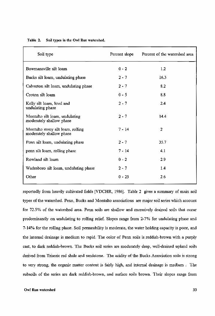
Table 2. Soil types in the Owl Run watershed.

Soil type Percent slope Percent of the watershed area

Bowmansville silt loam 0-2 1.2

Bucks silt loam, undulating phase 2-7 16.3

Calverton silt loam, undulating phase 2-7 8.2

Croton silt loam 0-5 8.8

Kelly silt loam, level and 2-7 2.4 undulating phase

Montalto silt loam, undulating 2-7 14.4 moderately shallow phase

Montalto stony silt loam, rolling 7-14 2 moderately shallow phase

Penn silt loam, undulating phase 2-7 35.7

penn silt loam, rolling phase 7-14 4.1

Rowland silt loam 0-2 2.9

Wadesboro silt loam, undulating phase 2-7 1.4

Other 0 - 25 2.6 reportedly from heavily cultivated fields [VDCHR, 1986]. Table 2 gives a summary of main soil

types of the watershed. Penn, Bucks and Montalto associations are major soil series which account

for 72.5% of the watershed area. Penn soils are shallow and excessively drained soils that occur

predominantly on undulating to rolling relief. Slopes range from 2-7% for undulating phase and

7-14% for the rolling phase. Soil permeability is moderate, the water holding capacity is poor, and

the internal drainage is medium to rapid. The color of Penn soils is reddish-brown with a purply

cast, to dark reddish-brown. The Bucks soil series are moderately deep, well-drained upland soils

derived from Triassic red shale and sandstone. The acidity of the Bucks Association soils ts strong

to very strong, the organic matter content is fairly high, and internal drainage is medium . The

subsoils of the series are dark reddish-brown, and surface soils brown. Their slopes range from


2-7%. The Montalto soils were derived from fine-grained Triaasic diabase with medium to strong

acidity. The slopes of the series range from 2-14%. The soils are moderately well supplied with

Organic matter and plant nutrients so that they are relatively fertile. Internal drainage is medium and

erosion ranges from none on forest to moderate on agricultural areas [SCS, 1956]. The Montalto

soils are moderately shallow and relatively dark and, therefore, warm and dry in the spring for early

plowing. A spatial distribution of major soils types of the watershed is given in Figure 5.

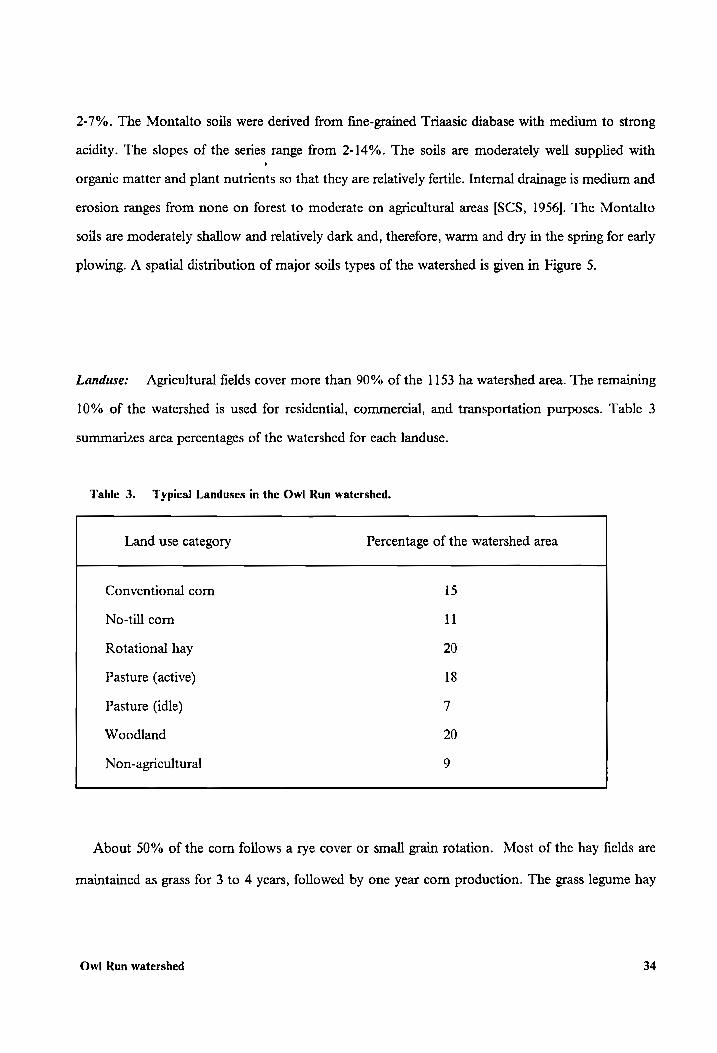
Landuse: Agricultural fields cover more than 90% of the 1153 ha watershed area. The remaining

10% of the watershed is used for residential, commercial, and transportation purposes. Table 3

summarizes area percentages of the watershed for each landuse.

Table 3. Typical Landuses in the Owl Run watershed.

Land use category Percentage of the watershed area

Conventional corn

No-till corn

Rotational hay

Pasture (active)

Pasture (idle)

Woodland

Non-agricultural

15

1]

20

18

7

20

About 50% of the corn follows a rye cover or small grain rotation. Most of the hay fields are

maintained as grass for 3 to 4 years, followed by one year corn production. The grass legume hay


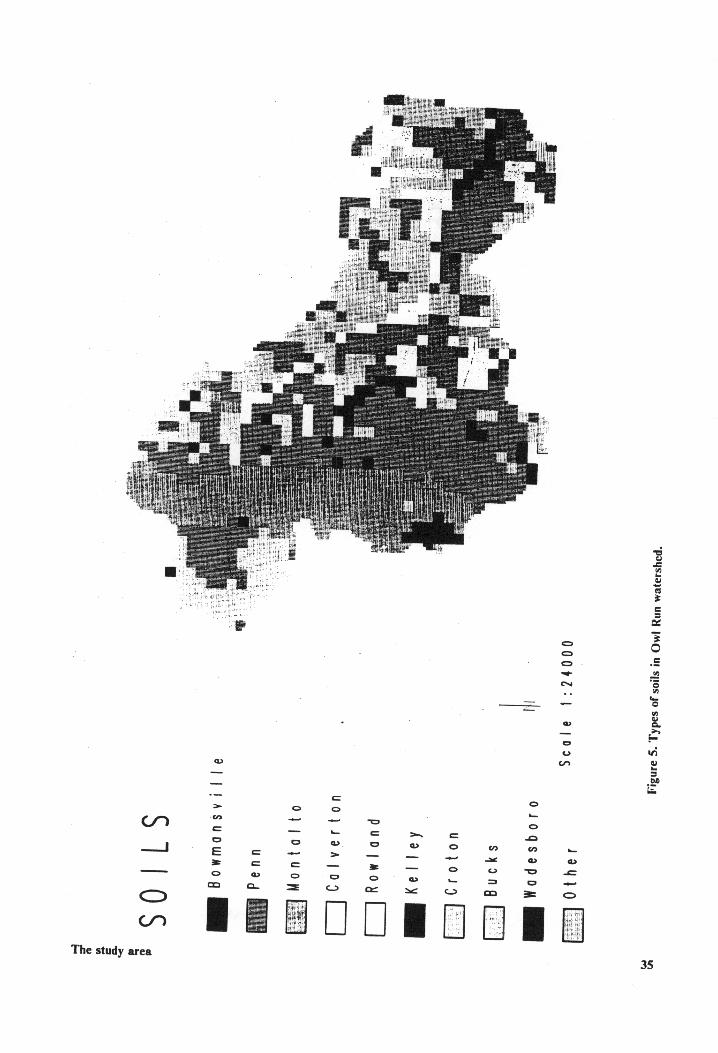
“POYsiayEM UNY

[MO UI

Sjlos yo

sadky °¢

ainsi

000%Z:1 aoa

72410 i

o1oqgsapoy

syong[-_]

vojyoin [|

Coijoy

puojmoy[

|

Oo vo,saajog[_ |

0} | 0}u0oK

uuad

a;iissuownog

fe

5110S

35 The study area

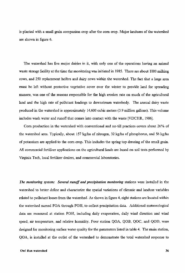
is planted with a small grain companion crop after the corn crop. Major landuses of the watershed

are shown in figure 6.

The watershed has five major dairies in it, with only one of the operations having an animal

waste storage facility at the time the monitoring was initiated in 1985. There are about 1000 milking

cows, and 250 replacement heifers and dairy cows within the watershed. The fact that a large area

must be left without protective vegetative cover over the winter to provide land for spreading

manure, was one of the reasons responsible for the high erosion rate on much of the agricultural

land and the high rate of pollutant loadings to downstream waterbody. The annual dairy waste

produced in the watershed 1s approximately 14,600 cubic meters (3.9 million gallons). This volume

includes wash water and runoff that comes into contact with the waste [VDCHR, 1986].

Corn production in the watershed with conventional and no-till practices covers about 26% of

the watershed area. Typically, about 157 kg/ha of nitrogen, 32 kg/ha of phosphorus, and 56 kg/ha

of potassium are applied to the corn crop. This includes the spring top dressing of the small grain.

All commercial fertilizer applications on the agricultural lands are based on soil tests performed by

Virginia Tech, local fertilizer dealers, and commercial laboratories.

The monitoring system: Several runoff and precipitation monitoring stations were installed in the

watershed to better define and characterize the spatial variations of climatic and landuse variables

related to pollutant losses from the watershed. As shown in figure 4, eight stations are located within

the watershed named POA through POH, to collect precipitation data. Additional meteorological

data are measured at station POH, including daily evaporation, daily wind direction and wind

speed, air temperature, and relative humidity. Four station QOA, QOB, QOC, and QOD, were

designed for monitoring surface water quality for the parameters listed in table 4. The main station,

QOA, is installed at the outlet of the watershed to demonstrate the total watershed response to


Mm— ar

SJ i <=

cc

oO — =

—_—_-+

<—<l-— ©

Hj =m

The study area

So

te

=>

~

=

eo

ke

m

<

I

=

°o

=

Qa

Oo

—

oO

@

—

=>

—

wn

o

a.

nn

Ee o @ —

~ wn

nm

@

—

o

~~

c

Ss

Oo

co

~~

@

uw

Scale

1:24000

Figure

6. Major

landuses

of Owl

Run

watershed.

37

BMP implementations. Seven private groundwater wells were used to monitor groundwater qual-

ity, as GOE, GOF, GOG, GOH, GOI, GOJ, and GOK (Figure 4).

Five data layers of the watershed, elevations, stream networks, watershed boundaries, soil types,

and general landuse, were digitized and stored in raster format into a database. The management

of the database, including digitization, error checking and correction of the data were performed

by the Virginia Geographic Information System (VirGIS) laborary, located in the Agricultural En-

gineering Department at Virginia Tech [Shanholtz, et al., 1987]. Soil and landuse survey program

of the monitoring project provided the basis for monthly landuse survey and quarterly soil sampling

on the watershed. The landuse survey provides a comprehensive documentation of agricultural and

animal waste management practices implemented on the watershed.


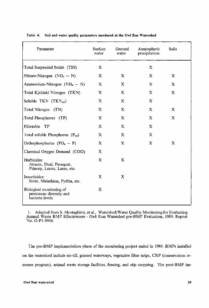
Table 4. Soil and water quality parameters monitored at the Owl Run Watershed

Parameter Surface Ground Atmospheric Soils water water precipitation

Total Suspended Solids (TSS)

Nitrate-Nitrogen (NO; — N)

Ammonium-Nitrogen (NH, — N)

Total Kjeldahl Nitrogen (TKN)

Soluble TKN (TKNga1)

Total Nitrogen (TN)

Total Phosphorus (TP)

Filterable TP

Total soluble Phosphorus (Pyo1)

~ Mm

Mm MM

MM

MOK

~ ~

KX KH

KH

KH

MH MH

KM OM

Orthophosphorus (PO, — P)

Chemical Oxygen Demand (COD)

~ Mm

KM MH

KH Mm

MH KM

mR

MK OK

OM

Herbicides: Atrazin, Dual, Paraquat, Princep, Lorox, Lasso, etc.

Insecticides: x 4 Sevin, Malathion, Pydrin, etc.

Biological monitoring of x protozoan diversity and bacteria levels

1. Adapted from S. Mostaghimi, et al., Watershed/Water Quality Monitoring for Evaluating Animal Waste BMP Effectiveness - Owl Run Watershed pre-BMP Evaluation, 1989. Report No. O-P1-8906.

The pre-BMP implementation phase of the monitoring project ended in 1989. BMPs installed

on the watershed include no-till, grassed waterways, vegetative filter strips, CRP (conservation re-

source program), animal waste storage facilities, fencing, and stip cropping. The post-BMP im-


plementation phase of the project will continue to be monitored for several years to evaluate both

the short term and long term impact of the practices.

The Owl Run watershed monitoring project makes it possible to develop, verify, or validate

various nonpoint source pollution models with the abundant meteorological, hydrological, land use,

soil and water quality data available. The database management system established by the project

can greatly enhance the usability of the data collected for model verification and BMP evaluations.


Model Validation

It is necessary to validate a model before applying it to a specific area. Validation of a model is

defined as demonstrating its applicability by identifying the accuracy of the parameters selected for

the study area. Complete model validation requires testing over the full range of conditions for

which the model simulates [Hern, et al., 1987]. There are generally two major steps involved in

model validation. First, the correctness of the selected model parameters needs to be determined

by comparing model predictions with measured watershed response from a series of record, and

calibrating the selected input parameters, if necessary. The second step is to use the selected pa-

rameter set (or calibrated parameters) on a different series of record and determine simulation errors

(Haan, et al., 1982; Young and Alward, 1983]. Therefore, two independent series of events need to

be provided to carry out this procedure.

The purpose of this chapter is to demonstrate the AGNPS applicability to Virginia Piedmont

conditions by comparing its predictions with data collected from the Owl Run watershed. As re-

quired by the validation procedure, two series of storms were selected from 1987, and 1988 records.

The 1988 series of storms were used for evaluating the selected input parameters. The parameters

obtained were then used on the second series (1987) with the same landuse and management

conditions. The simulation results and the corresponding observed data are plotted against each

other to present a visual view of the model performance. Both visual comparisons and statistical

Model Validation 41

analysis were performed on simulation results of both storm series to evaluate the model’s appli- —

cability.

Selection of the storm events

Over 100 storm events are observed on the Owl Run watershed each year. Among these events,

only about 40% produced measurable runoff. The precipitation amounts for each of these storms

are generally larger than 7 mm [Mostaghimi, et al., 1989]. For the purpose of data selection and

analysis, storms greater than 7 mm in rainfall amount are defined as primary storms. To meet the

requirement of statistical analysis and model validation, 11 of the 37 primary storm events which

occurred during 1988 were selected randomly throughout the year for parameter evaluation and

model testing. 12 primary events from 1987 were also selected, using the same procedure as 1988,

to carry out the model validation procedure.

Preparation and evaluation of input parameter values

Over 20 input parameters for each cell are needed for AGNPS simulations. Of these parameters,

some of them maintain the same value throughout the year and are not time dependent. These

values include topographic data such as land slope, slope direction (aspect), channel slope, channel

side slope, and soil properties including soil textures, erodibility factors, and hydrologic soil groups.

Other parameters such as curve number, cropping factor and Manning’s roughness coefficient are

functions of crop types and other surface cover and vary with the time of the year.

The procedure used for preparation and evaluation of parameters in this study consisted of

two steps. First, the input parameters for a watershed were selected homogeneously throughout the

year, i.e. the parameters were assumed to be the same for different crop stages. This set of param-

Model Validation 42

eters depicts the average conditions on the watershed throughout the year. A series of events were

simulated and the results were compared with the data collected from the Owl Run watershed.

The model with homogeneous parameters underpredicted watershed responses for those storm

events occurred during dormant season, and overpredicted the responses for the events during

growing season. The second step was to divide the whole year into two different seasons, dormant

and growing, in an attempt to refine the input parameter values. The period from May 15 through

October 15 was defined for Owl Run as the growing season, and the rest of the year as dormant

season. Input parameters with seasonal changes such as cropping factor in USLE, curve number,

Manning’s roughness coefficient, and surface condition constant were then prepared for the two

seasons.

As a distributed watershed model, the size of the cells in AGNPS needs to be selected carefully.

As mentioned in the literature review chapter, it takes about 20 minutes to collect and manage

necessary data for the preparation of input parameters for each cell [Young, et al. 1987; Koelliker

and Humbert, 1989]. The cell size for this study has to be selected carefully because the parameters

used in this study are treated manually. Feezor and Hirschi [1989] suggested that the smallest size

practical should be used to maintain the highest accuracy with AGNPS simulations. They used

one-hectare cell size as the basic size and compared the simulation results with that of other larger

cell sizes. The four-hectare size was found to cause an overall deviation less than 10 percent for the

results of the basic cell size for both sediment yield and nutrient loadings. A four-hectare cell size

was chosen for this study for the sake of both time-saving and necessary accuracy of the results.

Topographical parameters

Cell number, receiving cell number, land slope, slope shape, slope length, flow direction (aspect),

channel slope, channel side slope, and channel type indicator were obtained from 1:24000 scale

United States Geological Survey topographic map of Fauquire County, Virginia, which was

digitized into VirGIS database [Shanholtz, et al., 1987].

Cell number and the receiving cell number are used by the model to identify the locations of the

watershed behaviors. The other topographic parameters, together with the cell and receiving cell

Model Validation 43

numbers, are used by the model to route the runoff, sediment, and chemicals downstream and to

the watershed outlet.

Curve Number (CN)

The curve number is a key parameter used in SCS curve number method, which is adopted by

the hydrology component of AGNPS to estimate surface runoff volume. This parameter is a func-

tion of several variables including landuse, hydrologic soil group, and antecedent soil moisture

conditions. The landuse varies seasonally, the antecedent soil moisture condition varies from event

to event, while the hydrologic soil group remains constant. Curve numbers were determined using

the procedures outlined in the Engineering Handbook, Section 4 -- Hydrology [USDA-SCS, 1972].

A simple computer program was developed to calculate a CN for each cell based on landuse,

antecedent soil moisture condition, and soil property. With the incorporation of this software pro-

gram into AGNPS, the CN values in the input file of the model could be replaced by landuse, soil

hydrologic group, and antecedent soil moisture condition, which are available as different data lay-

ers of a typical GIS.

Average parameter values for growing and dormant seasons are 79 and 87, respectively, ranging

from 66 to 91, and from 71 to 94. Conditions used for selection of the parameters are given in

Table 5.

Cropping factor (C)

The Universal Soil Loss Equation (USLE) is used in the erosion component of the model as

described in the AGNPS chapter. The C factor used in USLE is closely related to crop types,

growing seasons, and the amount of residue left on soil surface. A detailed landuse monitoring

program is very helpful to determine the C value by using the classification tables in AGNPS User's

Manual (Version 3.5) [Young, R.A., et al., 1989]. The landuse data used in this study is the general

landuse map digitized into a VirGIS data base (Figure 6). Two basic sets of C values were prepared,

one for the dormant season, and the other one for growing season, as used in the hydrology

Model Validation 44

component. Conditions adopted for the two seasons and their average values were listed in Tables

5 6, respectively. The values are calculated by using the tables presented by Wischmeier and Smith

[1978] according to the conditions listed in Table 5.

Support practice factor (P)

The P factor is another parameter used in the USLE. This is a key parameter to reflect the im-

pact of various management practices on improving water quality related to nonpoint source pol-

lution. The P parameter is defined by Wischmeier and Smith [1978] as the ratio of soil loss with a

specific support practice to the corresponding loss with up-and-down-slope culture. The selection

of the factor is based on various conservation practices [Wischmeier and Smith, 1978] which are

related to the time of the year. For simulations of the events before 1989, when the pre-BMP phase

of the monitoring project ended, a value of 1 is used to represent the conditions during that period.

The support practices related to the P factor include contouring, contouring stripcropping, buffer

stripcropping, and terracing. Any of these practices can be simulated by the model for post-BMP

period using the procedures described by Wischmeier and Smith [1978].

Manning’s roughness coefficient (n)

This factor is used in sediment routing component of the AGNPS, in which the Bagnold stream

power equation is used to evaluate effective sediment transport capacity. Manning’s roughness co-

efficient is used in calculating the average velocity of flow in the equation. Roughness coefficients

for different landuse conditions for each storm were selected using the AGNPS User’s Guide for

channelized flow and overland flow. For those cells where there was no definable channel,

roughness coefficients appropriate for the landuse of the cells were selected for the main surface

condition. Average n values and their corresponding conditions for the two seasons used in this

study are also listed in Tables 5 and 6.

Model Validation 45

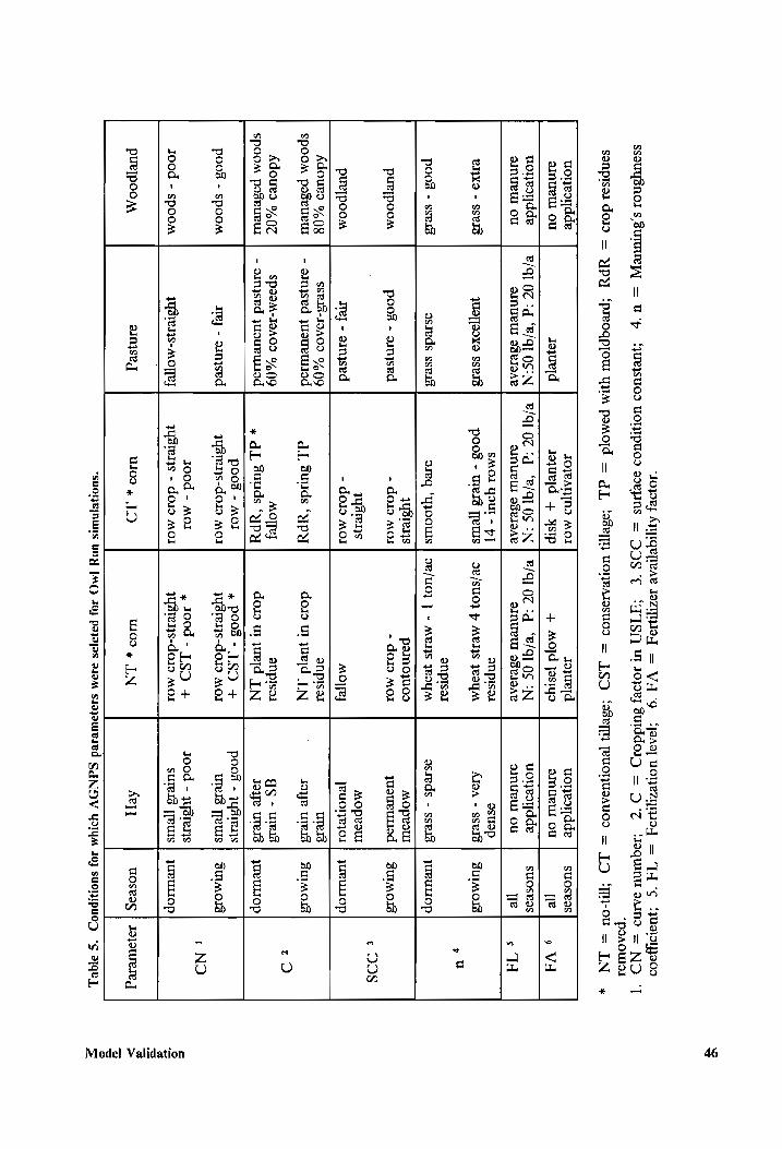
ssouysnol s 3uTduepy

= U

‘p ‘Jopuy

AUTIquieae Jez]

= VA

9 ‘JURISUOD

UOTIPUOS s9eJINS

= DOS

'C “ISN

ul sopry

suiddoiy =

7 7

{POAg] UONeZIWI

= Jy

‘¢ ‘yusroyjaoo

‘Joquinu sAInNd

= ND

‘PoAOUlal sonpisal

dolo =

Ypy

‘preoqpjow yUM

pomoyd =

Gg] ‘osely

UONRAIOsSUOD =

[SD ‘odefy

FeuONUDAUOD =

JD ‘qN-0uU

= IN

+

uoreoydde JOJEATNI

MOI Joyued

uolesydde |

suosvas omueUw

OU Jojur|d

Jojuejd +

ysIp +

Mod

Jasrys oimueul

ou Tre

9 VA

uoneoydde |

e/q] 07

:d ‘8/41

0S:N | ®/41

07 ‘d

“B/QT.0S -N |

®/Q1 07

ds ‘P/Q.

0S ¢N

uoneoydde |

suosvas oinueul

OU SINULUL

ISPIOAL OINUBULT

BdEIOAR SINUEUT

ddvIOAR oinueul

OU Te

s TA

SMOJ YOUI

- pf] anpiso1

osuop BI]X9

- sseId

JUST[INX9 ssid

poos - uresd

Tews |

9e/su0} p Mes

yeoyM AIOA

- sseId |

SUIMOIS U

v

onpisar pood

- ssvid

osieds sseid

oreq ‘Y}OOUIS |

9e/UO} |

- MeIIS

yeOUM asreds

- sseig |

juewop

1YysIeI4s poinojuos

MoOproul pur[poom

pood - s1injsed

- dolo

MOI - do1d

MOI yuoueued |

ZuImMols

¢ OOS

1Ysrens MoOpeoul

pur]poom Tre}

- ainjsed

- doid

MOI MOTTE}

Teuorejol |

yueWIOp

Kdoued % 08

SSBIS-INAOD (9

onpisos ureid

SpoomM paseuew

| - ainjsed

yuoueuod

d.L suuds

‘ypy dois

wt yueld

TN Jaye

ures | suimold

z Adours

% 07

SP9BM-I3AOD %()9

MOTTE} anptsol

aS - ures

Spoom podeurul

| - oInjsed

yuoueUod

+ dL

suuds ‘ypy

dois ut

yuejd TN

Joye utels |

jUeWIOp

pood - Mol

« poos

- SD

+ poos

- 1ysreNs

pood - spoom

Trey - oinysed

yystesys-do3o MOI

yysrerjs-dolo MOI

utlelg yfews |

SuIMoId

1 NO

Jood - Mos

» Wood

- JSD

4+ Jood

- jysress

Jood - spoom

yysresys- Moje} Wystels

- dod

MOI Wysteljs-do1o

MOI suTeid

yews |

jUeWIOp

pur[poon, oINjsey

uO) y LD

UWIOS » LN

Key] uoseag |

Jojoureleg

*‘SUOHZENUNIS UNY

JMO JO}

pazajas d4aM

SuaJoWIVIed GUNOV YY

10} suonipuo?

*¢ 31qe),

46 Model Validation

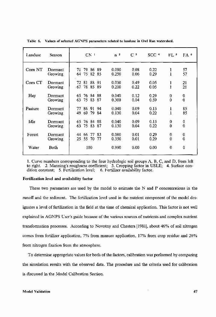
Table 6. Values of selected AGNPS parameters related to landuse in Owl Run watershed.

Landuse Season CN ! n ? C 3 SCC 4 FL5 FA 6

Com NT Dormant 71 79 86 89 0.090 0.08 0.22 l 57 Growing 64 75 82 85 0.250 0.06 0.29 l 57

Corn CT Dormant 72 81 88 9] 0.030 0.49 0.05 l 21 Growing -67 78 85 8&9 0.200 0.22 0.05 1 21

Hay Dormant 65 76 84 88 0.040 0.12 0.29 0 0 Growing 63 75 83 87 0.300 0.04 0.59 0 0

Pasture Dormant 77 86 91 94 0.040 0.09 0.15 1 85 Growing 49 69 79 84 0.130 0.04 0.22 l 85

Idle Dormant 65 76 84 88 0.040 0.09 0.15 0 0 Growing 63 75 83 87 0.130 0.04 0.22 0 0

Forest Dormant 44 66 77 83 0.080 0.01 0.29 0 0 Growing 25 55 70 77 0.350 0.01 0.29 0 0

Water Both 100 0.990 0.00 0.00 0 0 1. Curve numbers corresponding to the four hydrologic soil groups A, B, C, and D, from left to nght. 2. Manning’s roughness coefficient; 3. Cropping factor in USLE; 4. Surface condition constant; 5. Fertilization level; 6. Fertilizer availability factor.

Fertilization level and availability factor

These two parameters are used by the model to estimate the N and P concentrations in the

runoff and the sediment. The fertilization level used in the nutrient component of the model des-

ignates a level of fertilization in the field at the tume of chemical application. This factor is not well

explained in AGNPS User’s guide because of the various sources of nutrients and complex nutrient

transformation processes. According to Novotny and Chesters [1981], about 46% of soil nitrogen

comes from fertilizer application, 7% from manure application, 17% from crop residue and 20%

from nitrogen fixation from the atmosphere.

To determine appropriate values for both of the factors, calibration was performed by comparing

the simulation results with the observed data. The procedure and the criteria used for calibration

is discussed in the Model Calibration Section.

Model Validation ; 47

It is suggested by the AGNPS User’s Guide that, for a manure applied field, low fertilization

level (50 lb/ac N and 20 lb/ac P) for average manure application, and medium fertilization (100

Ib/ac N and 40 lb/ac P) for a heavy application of manure be assumed for the model input. Tables

5 and 6 list the average values for the manure applied fields and the conditions adapted for different

landuses, respectively, which were determined through calibration.

Fertilizer availability factor denotes the percent of fertilizer left in the top 1 centimeter of soil at

the time of the storm. This value changes with time because of the processes of chemical

volatilization, crop uptake, decay or attenuation, leaching to ground water, and losses to runoff

water. Therefore, the magnitude of this parameter is related to many factors such as different types

of cultivation activities, the methods of chemical application, meteorological conditions including

temperature, moisture, wind speed, amount and intensity of precipitation, or combinations of var-

10us conditions [Young, et al., 1985]. Wheras the only factor considered in the user’s manual for

determination of this availability factor is the type of cultivation activities. Detailed landuse data

is expected to make the parameters evaluated as realistic as possible. Values and corresponding

cultivation activities used for this study were determined by assuming that there are two cultivation

activities within each of the two periods selected for the year, representing average conditions for

that period. Minor adjustments for this parameter were also made through calibration (refer to

Calibration Section). Conditions and final values used are also listed in Tables 5 and 6, respectively.

Soil erodibility factor (K)

Some soil surveys include the soil erodibility factor, K, for different layers of the soils. For Owl

Run watershed, the latest version of soil survey is the Fauquir County Soil Survey published in

1956 [USDA-SCS, 1956]. This soil survey does not present the soil erodibility factors. The K factors

used for AGNPS input were identified by using the procedure outlined by Novotny and Chesters

[1981], which is based on organic matter content and textural classes of the soils. This is a simpli-

fication of the relationship developed by Wischmeier and Mannering [1969] on 55 soils in the

United States. The relationship is represented by an empirical equation with 24 variables (15 soil

Mode! Validation 48

properties and their combinations including organic matter content, aggregation index, thickness

of granular material, structure, antecedent soil moisture, etc.).

Surface condition constant (SCC)

This parameter is based on the condition of the landuse at the time of storms. This parameter

is used to make adjustments for the time it takes for overland flow to channelize in the sediment

and chemical routing components of the model. The values for various landuse and the two seasons

used in this study were obtained using the procedure similar to that of curve numbers outlined in

the AGNPS User’s Guide [Young, et al., 1985]. The conditions used for the determination of the

values in Table 5, and the selected values are listed in Table 6.

Chemical oxygen demand (COD) factor

The value of this factor is based on the landuse of the individual cells. It represents the average

COD concentration of the runoff from the cell. The AGNPS User’s Guide provides the values of

the factor for various landuses, which were based on estimates of background concentrations from

several northern states of the United States.

Statistical analysis

Errors from a variety of sources may be involved in modeling efforts. Measurement of observed

data, preparation of model parameters, and approximations and assumptions of physical relation-

ships adopted by the model are major sources of the errors. Wrong conclusions may be based on

these uncertainties. Statistical analysis provides a measurement of model accuracy by identifying the

total variation caused by the errors involved.

Model Validation 49

Several statistical methods are used in this study to evaluate the model performance and to

provide further understanding of the model’s applicability to Virginia’s conditions. The statistical

procedures used in this study include:

1. Regression analysis;

2. Root mean square error (rms);

3. Comparison of means between the observed and simulated results.

Regression analysis:

A simple linear regression line can be obtained by least square method

Y,;=a+bX;, +e; i= 1,2, oeeeee nN. (14)

in which Y; is the ith value of simulation; n is the number of simulations within a series; X; is the

observed value; a is the intercept, b is the slope of the regression line; and e;, is a random variable

representing errors around the regression line. A first impression can be obtained by drawing the

points of simulation and the regression line on a figure with X coordinate being the observed values

and Y coordinate the simulated values. Several statistics can be computed from the regression

Equation (14) [Haan, 1977]. The coefficient of determination, R?, is the ratio of the sum of squares

due to regression to the total sum of squares. It measures the ability of the regression line to explain

variations in the dependent variable. If the regression equation perfectly predicted every value of

Yi, or e;=0 for every i, the R? would be 1. On the other hand, if none of the variations in Y can

be explained by the regression equation, the value would be zero. The closer the R? is to 1, the

better is the relationship between simulated and observed values.

An estimate of the intercept and slope of the linear regression line can be obtained by using the

least square method. A slope of less than 1 means that the model underestimates the watershed

response, especially for large values, and a slope greater than | indicates overestimation. An neg-

ative intercept means that the model underestimates the watershed behavior, at least for small

events, and vice versa.

Model Validation 50

To test the significance of the slope and intercept, the null hypotheses on the intercept and the

slope can be written as:

Hp: a=0 (15 a)

Hp: b= 1 (15b)

where a is the intercept and b is the slope. The test statistics, a/S, and (b-1)/S,, are distributed

as student’s t with n-2 degrees-of-freedom. S? and S} are variances of the intercept and the slope,

respectively. These tests should be conducted as two-tailed tests with 5% probability significance

level on each side (t,j2=o05). A SAS simple linear regression program can be used to test

Hy:a = 0, Ho: b = 0, but not Hp:b= 1. Therefore hypothesis test on slope of 1:1 (or b= 1) was

performed manually in this study. Nonsignificant tests (null hypotheses are accepted) of equations

15a and 15b provide confidence to the modeler and demonstrates the applicability of the model

to the study area. In reality, it is impossible to obtain an exact 1:1 regression line with a zero in-

tercept. Evaluation of b, a, and R? provide additional levels of insight when comparing the model

prediction with the observed data.

While the coefficient of determination, R?, as mentioned above, provides a visual evaluation of

overall relationship between simulated and measured data, drawing confidence interval lines along

the obtained regression line gives the modeler or readers further information to evaluate the model

from the viewpoint of confidence intervals. For a certain level of confidence, the narrower the band

area between the confidence interval lines, the better the sample data represents the population.

The ultimate case is the coincidence of the two confidence interval lines on the regression line,

which means that there is no random error between the predicted and observed values.

The relationship used for calculating confidence intervals on the regression lines are given by:

L=y—S,t, —a/2,n—2 (16a)

Model Validation 51

Sy =sy/ In + (x- 9/9 (X—® (16 c)

where L and U are lower and upper confidence limits of the regression line, respectively; y and x

are coordinates of simulation points; s is the standard deviation of random variable e, in equation

(14); Xis the mean value of observed results; and « is the level of confidence [C.T. Haan. 1977].

Since our work is based on samples, all the statistic parameters (a, b, R?) are random variables

with certain probability distribution functions. The regression line is also a random variable as a

function of the random variables. For a continuous random variable, the probability that the vari-

able equals to a certain value is zero. The concept of confidence interval make it possible to evaluate

the variation of the errors involved in the simulation.

Root mean square (rms) error:

The root mean square error provides a pooled measure of differences between the observed and

simulated watershed response [Thomann, 1982]:

my 12 D; rms = Tn (17)

i=1

where D, is the difference between the observed and simulated values, and n is the number of pairs

of comparisons. The rms represents the standard error of estimate of model prediction and pro-

vides a direct estimate of model errors. The rms is also statistically well-behaved (identical, and

independently distributed as normal). If expressed as a ratio to the mean value of the observed or

simulated results data (whichever is smaller), the root mean square error represents a type of rela-

tive error and some researchers call this normalized quantity of the coefficient of variation (CV)

[Young, and Alward, 1983]. A relative error is especially useful when comparisons are being made

between different models. The disadvantage of the rms is that it does not reflect the impact of the

magnitude of variables.

Model Validation 52

Comparison of means between observed and simulated results:

A hypothesis test on the differences between observed and simulated values can be performed

under the null hypothesis: Hy, D = 0. Where D is the mean of the differences between the meas-

ured and predicted values [Thomann, 1982]. The test statistic, tors, is distributed as a student’s t

probability density function with a degree-of-freedom of n- 1:

D-—d =-—_—~T oT _ 18 lobs S/ TAL (18)

where d is the true difference expected between model prediction and the observed values which

is assumed to be zero, and S isa pooled value of the standard deviations of simulated and meas-

ured data. A significant result of this test (the null hypothesis Hp, D = 0 is rejected) at certain level,

say 5%, means that there is some apparent difference between the model prediction and the meas-

ured watershed response. A nonsignificant result (accepted the null hypothesis) gives us some con-

fidence that there is not enough evidence to criticize the overall model prediction.

All the three procedures mentioned above were used to validate the applicability of the model

to the study area. These methods evaluate the model credibility from different statistical viewpoints.

The rms error assess the overall model credibility by providing direct measure of model errors. The

test for comparison of means answers the question whether the difference between the simulation

results and the observed data is statistically acceptable. The parameters involved in the simple linear

regression procedure measure the errors related to the magnitude of the water quality problem, and

give the confidence intervals on the simulation results.

For hypothesis test problems, the criteria used to validate models are within the framework of

statistical analyses [Yang and Alward, 1983; Thomann, 1982]. A 5% significance level is widely

agreed to be reasonable to determine the validity of models. For direct error estimate procedures,

the criteria used by some researchers [Hedden, 1986] are: a) for screening applications, the model(s)

should be able to replicate observed field data within an order of magnitude; and b) for site-specific

applications, the prediction of the model(s) should be able to match the measured data within a

factor of two. Nevertheless, some scientists indicate that the site-specific criteria might not be met

Model Validation §3

easily by even the best models using carefully measured site-specific parameters [Smith, M.C., et

al., 1989].

Calibration

Calibration of AGNPS simulation was performed to closely approximate the observed runoff

volume, sediment yield, and nutrient loadings from the watershed. Such calibration allows for rea-

sonable estimate of input parameters for the model. Relevant parameters for model calibration

included curve number in the hydrology component; C factor, surface cover condition factor, and

Manning’s roughness coefficient used in soil erosion and sediment transport component; and

fertilization level and fertilizer availability factors in chemical loading component of the model.

Because of the error accumulation from runoff and sediment yield to nutrient loadings, the ac-

curacy of the hydrology and sediment simulations will influence the nutrient loading component.

Therefore the calibration procedure was performed on the hydrology, soil erosion and sediment

transport, and then the nutrient loading components.

These parameters were calibrated using the 1988 data series and the results were evaluated by

using the statistical measures and criteria mentioned previously in this section. The parameters were

adjusted according to the sensitivity analysis made by Young et al. [1985]. Various tables for de-

termination of the parameters collected in the AGNPS user’s manual were used to assure that the

parameters were adjusted within reasonable ranges. Once the selected parameter were calibrated to

within the satisfactory criteria, they were used for the 1987 data to evaluate the results using the

same statistical procedures. All of the calibrated input parameter values were realistic and within the

published ranges. Conditions and the corresponding adjusted parameter values are listed in Tables

5 and 6, respectively.

Model Validation 54

Results and discussion

The procedures outlined for model validation required simulations to be performed on both

1987 and 1988 data series selected for this study. The magnitude and date of occurrence of the se-

lected storm events are listed in tables 7 and 8 for the two series, respectively. The model input

parameters were prepared for both the growing season and the dormant season as defined previ-

ously in this chapter. The growing season parameter set was used to simulate those events occurred

during the crop growth period in the area, and the dormant season set was used for those events

occurred during the rest of the year.

All the three statistical methods explained in previous section were used on the two series of

storms. The parameters selected for the first series (1988) were tested by these methods and cali-

brated to the measured data. Simulations were then performed for 1987 events and the results were

tested by the same statistical procedures. The root mean square errors (rms) were examined first

because the corresponding relative error (coefficients of variation, CV) can be used to compare di-

rectly with the criteria suggested by some investigators [Hedden, 1986]. As defined in equation (17),

rms represents the overall average error between the observed and simulated results. The CV is the

ratio of rms to the observed or stmulated mean value (whichever is smaller). Therefore, the criterion

of within “a factor of two” will be satisfied when the ratio is less than 1 for site specific stimulations,

and the criterion of within “an order of magnitude” will be met when the CV value 1s less than 9.

According to these criteria [Hedden, 1986; Smith, et al., 1989], if the model simulates the watershed

response within a factor of two, the simple linear regression procedure and testing on differences

of means will give further confidence of the model credibility. When the relative error is outside of

a factor of two (CV is greater than 1), the simple linear regression analyses and the tests on means

can be used to diagnose the simulation problems.

Simulation results and direct comparisons with the observed data for runoff volume, peak flow

rate, sediment yield, total nitrogen, and total phosphorus concentrations at the watershed outlet,

are tabulated in tables 7 and 8 for 1988 and 1987 data sets, respectively. The two tables also include

Model Validation 55

values of root mean squares, coefficient of variation and parameters of simple linear regressions

(intercept, slope, and coefficient of determination). Test results on the intercept, slope and differ-

ences of means for various parameters are listed in tables 9 and 10 for 1988 and 1987 data sets,

respectively. Simulation results for the two storm series are also plotted against the observed data

in figures 7 through 11 for 1988 series, and figures 12 through 16 for 1987 series. Regression lines

and 95% confidence intervals along the lines are also plotted in the figures corresponding to each

of the parameters.

The runoff volumes predicted by the model compared favorably with the observed data. As

shown in figure 7 and figure 12 (runoff volume simulations for 1988 and 1987), simulation points

are well distributed along the regression lines, with intercepts and slopes being nearly zero and 1,

respectively. The confidence interval along the regression lines lie very close to the regression lines.

These results indicate that the regression lines, which are random variables, will fall between the

interval lines, 95% of the time. The relative errors evaluated in terms of CV values were 0.15, and

0.29 for 1988 and 1987 (tables 7 and 8), respectively, well within the criterion of “a factor of two”.

R? values of the two series presented in tables 7 and 8 (0.99 and 0.97, respectively) are large enough

to demonstrate suitability of the relationship used in the hydrologic component of the model. The

hypotheses of zero intercept and 1:1 slope were accepted at the 5% significance level (tables 9 and

10). This indicates that the simulation results consistently agreed with the observed data. Tests on

the means of simulated and measured runoff showed no significant differences (tables 9 and 10) so

that the hydrology component was validated with further confidence.

Peak flow rates were generally overpredicted by the model. The overall relative errors (expressed

by CV) were 1.02 and 1.39 for 1988 and 1987, which were just over the “a factor of two” criteria.

The Discrepancies between the observed and simulated peak flow rates increase proportionally with

the magnitude of the storm events. Slopes of 1.39 and 1.55 were computed by the regression ana-

lyses for 1988 and 1987 events, respectively, which means the error increases proportionally with

the magnitude of the storms. Hypothesis tests on differences between the mean values of observed

peaks and simulated peaks were rejected at the 5% significance level, indicating that significant er-

rors do exist between the simulated and observed peak flow rate. The discrepancies between the

Model Validation 56

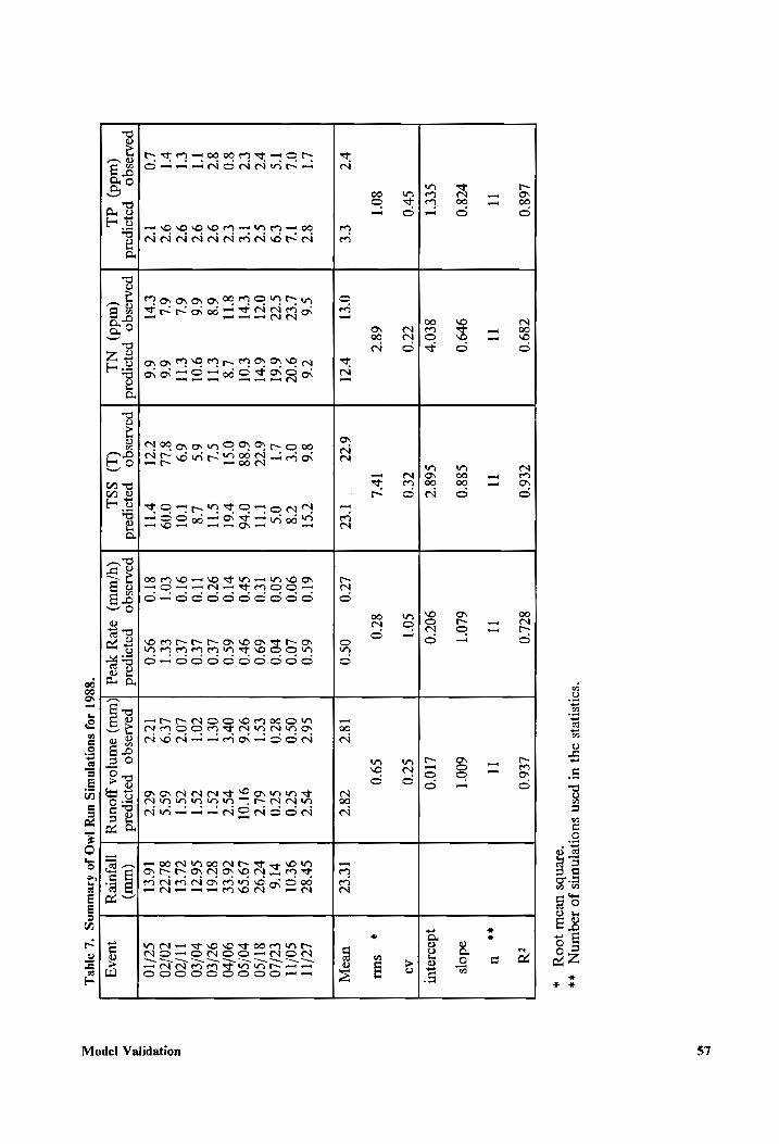
"SOI]SIILIS OY}

Ul posn

SUOTIEINUNS JO

JOQUINN, 4x

‘arenbs uesul

jooy sg

L680 €89°0

c£6'0 8cL'0

Lt60 cu

i a

Tl I

I ee

«OU

$780 979'0

$83°0 6L0'1

600°T adoys

Stel 8c0'P

$68°C 90¢'0

L100 ydoorayur

sv c0

ce'0 sol

$c0 AD

801 68°C

wl

8c'0 $9°0

+ SUE

vC ee

O¢T vl

6CC Tt?

Le0 0s°0

I8'¢ C8

Tee? hae Al

Lil 8C

$6 6

8°6 cSt

610 6$°0

S6C bs'C

Sv'8C LeU

OL VL

Lee 9°0¢

Oe o8

90°0 L0°0

0s°0 sc0

9¢°01 SO/TT

Vs C9

St? 66]

Li 0s

S00 v0'°0

8c'0 sc0

vl'6 €z/LO

ve S?

OCI 6 FI

6¢C TIT

T¢°0 69°0

cs] 6L°C

ve'9C 81/50

4 Ve

trl COI

688 076

sv'0 90

906 9TOl

L£9°S9 0/50

80 ec

STT L’8

O'sT y6l

v10 650

Ore bse

COLE 90/r0

8°C 9¢

68 Tl

CL ST

9¢°0 Lt0

orl cs

87 6l 9¢/€0

Ul 97¢

66 9°01

6¢ L’8

110 Lt0

col cs'T

s6?cl 70/0

eT 97C

6L Cll

69 TO!

910 Le

LOC cs]

cL el 11/Z0

bl 97

64 66

SLL 0°09

£01 cel

Leo 69°

8L°CC 70/20

L0 Ve

trl 66

cel tt

81°0 9$°0

1e?c 6C'C

lot! SZ/10

pearlssqo =

pajyoipaid |

poarosqo payorpoid |

poasasqo =

payotpaid |

poarosqo = poyorpaid

|

paarosqo payotpaid

(wut) (uidd)

dL (add)

NIL (L)

SSL (q/urux)

oyey Yeog

[(urw) surnjoa

Houny | [eyurey

qwoaq

S86] 40)

SuOeNUNTS

UNY JAG

jo ArewuNS

+f 3IqRy

57 Model Validation

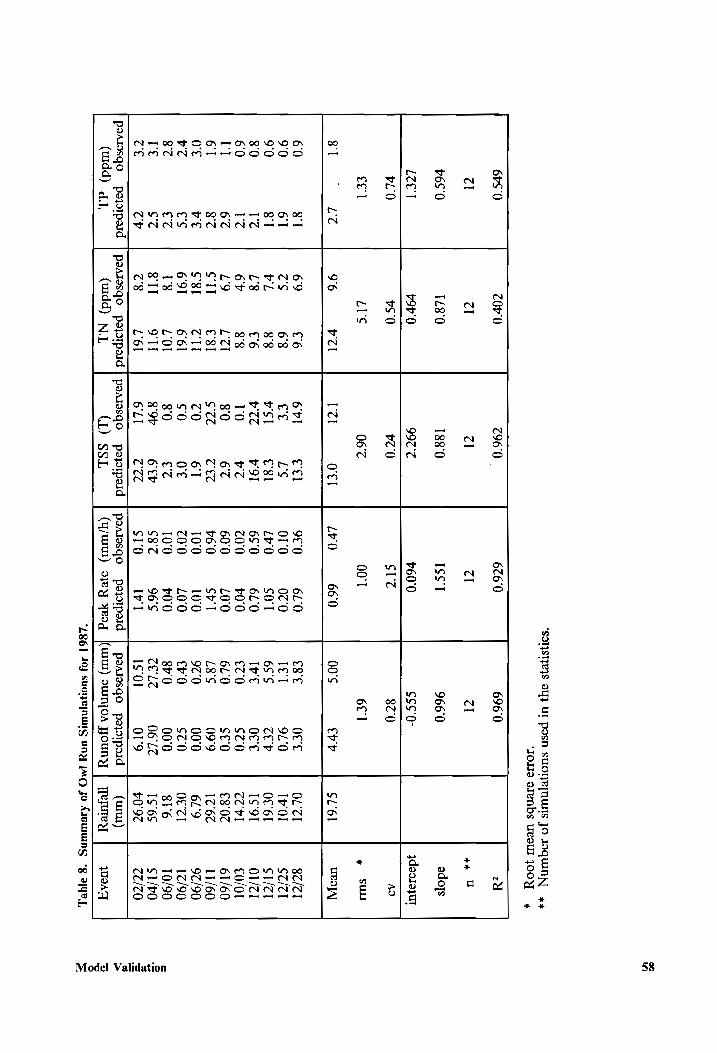
"SOIISI]IS SY}

Ul Posn

SUOTLINUNS JO

JOQUINN yy

‘1019 alenbs

uUedUT JOOY

sy

6bS'0

cor 0 €96'0

6260 696'0

ca

cl cl

cl cl

cl +a

U

v6s'0 TL8°0

188°0 Iss]

9660 adojs

Lev'l v9v'0

990°C 760°0

$s¢'0- ydaorayut

bl0 ps0

vc0 sl?

870 AO

cel LIS

06°C 001

6t'l +

SUL

81 "

Le 9°6

a | Vel

Otel LV0

66:0 00'S

tvy SLol

uUes}Al

60 8'T

69 €'6

641 eel

9¢°0 6L'0

csc Ore

OLCl 87/71

9°0 61

cS 68

et Ls

O10 0c°0

lel 9L°0

Ty'ol S7/Z1

9°0 8]

vl 38

vst esl

LPO sol

6S°S cov

Ot él

S1/Z1 80

Ve L’8

€'6 VCC

vol 6S°0

6L°0 Ive

Oe

Iso] O1/ZI

60 Ve

oh 8°8

10 VC

c0'0 v0'°0

tc0 sc0

co vl €0/01

UI 6C¢

Lg Ll

80 6¢

60°0 L0°0

6L°0 seo

£30

61/60 61

8c ST

€31 St

CLT v6'0

svi L3S

09°9 1C'6¢

11/60 oe

ve $31

cll c0

61 10°0

100 9¢°0

00°0 6L°9

97/90 v?

t's 691

661 SO

o€ c0'0

L0°0 tr

$c 0 OCC]

1Z/90 8

C7? V8

L0l 80

4 100

p00 8r0

00°0 816

10/90 Ve

sc STT

91] 8 9P

6 tP S8C

96'S COL

06°L7 1$°6S

S1/b0 cE

CV C8

L’6l 6LI

CCC S10

Tvl $01

O19 b0'9¢

77/70 pealasqo

= pajyoiposd |

paarosqo

payorpoid | paarosqo

§ payotpoid

| psalosqo

= poyipaid |

poarlasqo payorpaid

(ur)

(udd) dL,

(add) NIL

(L) SSL

(y/um) oyey

yeog [(wmur)

sunjoa youny |

yeyurey WoAq

“L861 40)

SUNT |NUNS

UNY [IMG

Jo ArewUINS

*g age),

58 Model Validation

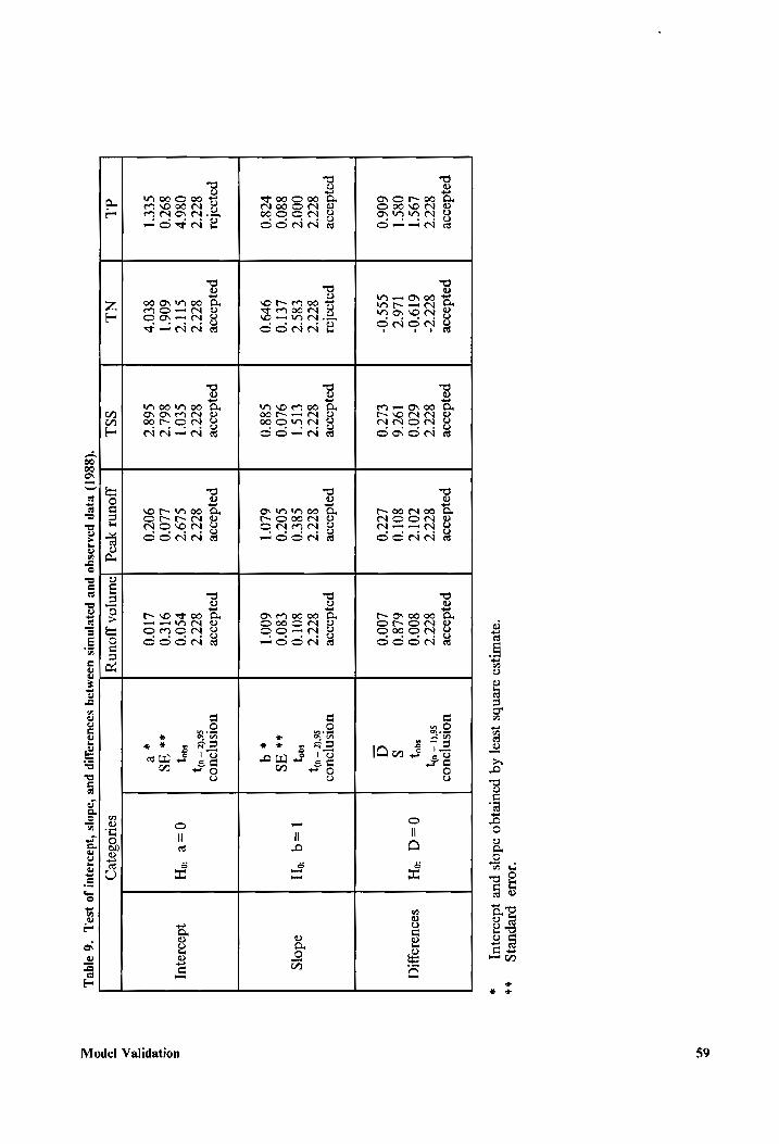
‘Joa prepuejig

, ‘9yeuryso

asenbs ysea]

Aq pouteygo

odojs pure

4da0I9}u] * *

pardasor paidasoe

pajdasoe poidasoe

poidaooe uoIsnpDUeS

877? 8CC'C-

82?

8CCC 8CCC

st — wy

L9oS'T 619°0-

620°0 cor?

800°0 ae)

0=d

“H SSOUsIOWI

O8s'T IL6¢

19C'6 8010

6L£8°0 Ss

606°0 $ss'0-

€£o'0 Lew0

£00°0 d

poidesse popalar

poidasoe pojdascor

psydasoe uOoTsnpIUOS

8CCOC 8CC'C

827? 8CCC

8CC'C so

Oy 000°

€8S°C els]

$8¢'0 8010

mY 1=4

*H adojs

8800 Ltl0

9L0°0 $070

£80°0 ##

AS vcs 0

979°0 $83°0

6L0°1 600°T

#4

poolor poidsooe

poidosoe poidasoe

poidsoo" UOIsNpIUOS

8CC'C 8CCC

8CCC 8CC'C

8CCC SoC

My 086°

SII? Sc0'l

SL9C bS0'0

m4 O="

*H ydooraqu]

8970 6061

86L°C LLO0

91C'0 +e

AS SECT

8t0'P S68°C

90¢'0 L100

#8

dL NL

SS.L youn

yeag jeumyoa

youny

SoU089}e7)

(8861) Byep

pIasasqo pus

poyejnus uIaMjJoq

SaDUJIAYIP pue

‘adojs 4ydad49}UI

Jo SIE

°G F/G.

59 Model Validation

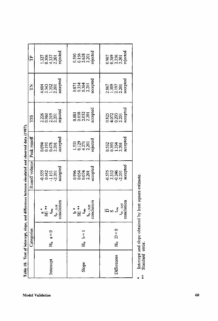
“IONS

prepuejg

**

‘syeutyso orenbs

yseaq Aq

pouteyqo adojs

pue ydoo0ju]

*

pewpalas pordasoe

poidaooe paidasoe

paidasse woIsn[auOS

1l0c¢ 10e°¢

10c¢°¢ 10c'¢

T0c'¢- sot

My 9S"

L6I'C £0¢'0

vSe'l 9¢e°0-

°y 0=d

*H SsoustIonic]

68¢°0 60¢'T

CLO'P €6£°0

CEE N)

L060 L98'C

$80

ces 0 SLS'0-

d

psyoatar poydesor

poidasoe poyolar

poidaooe uolsnjouos

1077 1077

10¢°7 102¢°7

1077 ee

8¢9°C v9t'0

cSO'C ILep

PL0'0 oa

=4 “H

adojs 9S1°0

pse0 8S0°0

610

vs0'0 «4

AS 06$°0

1L8°0 188°0

Iss'T 966°0

#4

poayolas poidssoe

popolar paidssoe

poidasoe uOIsn[IUOD

10c°@ 10¢°¢

10c¢ 10¢'?@

10¢'¢- soe

wy LeCy

cool 6I€¢

8Lr'0 Ist T

-

oy O=?

°H ydoo19}U]

90¢°0 tree

096°0 €61°0

C80

+4 AS

Lcee'l v09'P

9¢CC ¥60°0

Ss¢'0- ©

dL NL

SSL youn

yeog jawnyoa

jyouny soogaye7)

(L861) ByEp

paasasqgo pus

przEjNWIs UIIaMj}2q

SIdUdIIIp puw

‘adojs 4ydad49}uUL

Jo ISAT,

“OT FIG

60 Model Validation

simulated and observed peak runoff rates can be partially due to the empirical nature of the re-

lationship used in AGNPS for calculating the peak rates. The empirical equation used to predict

peak flow in AGNPS (equation (5) in this study) was developed using data from 304 storms oc-

curred on 56 watersheds located in 14 states [Knisel, et al., 1980]. The watershed sizes ranged from

less than 100 ha to over 6000 ha, and the exponents for drainage area A and runoff volume Q in

equation (5) vary with the sizes of watersheds. The current version of AGNPS does not have the

capability of adjusting these two parameters for specific applications.

The erosion and sediment yield predictions of the model agreed well with the measured data.

The coefficients of variation, CVs in tables 7 and 8 for TSS (total suspended sediment), were quite

small and easily within “a factor of two” (less than 1). The coefficients of determinations, R? , were

0.94 and 0.96 for 1988 and 1987, respectively. This simply means that the random errors are only

6 and 4 percent of the total variations. These values of R? for sediment yield are smaller than those

for runoff because errors within the hydrology components of AGNPS could have been accumu-

lated into the erosion and sediment routing components. The hypotheses that the intercepts of the

regression lines are zero were accepted for both data series, however the test on slope for the 1988

data was rejected. Therefore, it can be concluded that there are some minor errors which associated

with AGNPS predictions of TSS increase proportionally with the storm magnitude. The overall

differences between the simulated and measured data of the two series were not significant (Tables

9 and 10). This demonstrated further that the sediment yield component is acceptable for our

study area. Large differences between simulated and observed sediment yield can be found for some

big storms occurred during the two years (table 7). The energy intensity value EI, used in the

USLE, may not be evenly distributed spatially throughout the watershed. The current version of

AGNPS does not take into account the spatial variation of the EI values within a watershed. The

model uses only one EI value for the whole watershed. This uncertainty was incorporated into the

modeling results because Thiessen average EI values were used as input. Errors from hydrology and

soil erosion and sediment transport components were accumulated into the following nutrient

loading component.

Model Validation 6l

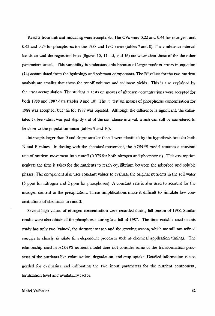
Results from nutrient modeling were acceptable. The CVs were 0.22 and 0.44 for nitrogen, and

0.43 and 0.74 for phosphorus for the 1988 and 1987 series (tables 7 and 8). The confidence interval

bands around the regression lines (figures 10, 11, 15, and 16) are wider than those of the the other

parameters tested. This variability is understandable because of larger random errors in equation

(14) accumulated from the hydrology and sediment components. The R? values for the two nutrient

analysis are smaller that those for runoff volumes and sediment yields. This is also explained by

the error accumulation. The student t tests on means of nitrogen concentrations were accepted for

both 1988 and 1987 data (tables 9 and 10). The t test on means of phosphorus concentration for

1988 was accepted, but the for 1987 was rejected. Although the difference is significant, the calcu-

lated t observation was just slightly out of the confidence interval, which can still be considered to

be close to the population mean (tables 9 and 10).

Intercepts larger than 0 and slopes smaller than 1 were identified by the hypothesis tests for both

N and P values. In dealing with the chemical movement, the AGNPS model assumes a constant

rate of nutrient movement into runoff (0.075 for both nitrogen and phosphorus). This assumption

neglects the time it takes for the nutrients to reach equilibrium between the adsorbed and soluble

phases. The component also uses constant values to evaluate the original nutrients in the soil water

(5 ppm for nitrogen and 2 ppm for phosphorus). A constant rate is also used to account for the

nitrogen content in the precipitation. These simplifications make it difficult to simulate low con-

centrations of chemicals in runoff.

Several high values of nitrogen concentration were recorded during fall season of 1988. Similar

results were also obtained for phosphorus during late fall of 1987. The time variable used in this

study has only two ‘values’, the dormant season and the growing season, which are still not refined

enough to closely simulate time-dependent processes such as chemical application timings. The

relationship used in AGNPS nutrient model does not consider some of the transformation proc-

esses of the nutrients like volatilization, degradation, and crop uptake. Detailed information is also

needed for evaluating and calibrating the two input parameters for the nutrient component,

fertilization level and availability factor.

Model Validation 62

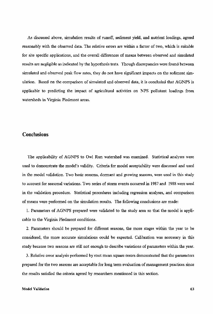
As discussed above, simulation results of runoff, sediment yield, and nutrient loadings, agreed

reasonably with the observed data. The relative errors are within a factor of two, which is suitable

for site specific applications, and the overall differences of means between observed and simulated

results are negligible as indicated by the hypothesis tests. Though discrepancies were found between

simulated and observed peak flow rates, they do not have significant impacts on the sediment sim-

ulation. Based on the comparison of simulated and observed data, it is concluded that AGNPS is

applicable to predicting the impact of agricultural activities on NPS pollutant loadings from

watersheds in Virginia Piedmont areas.

Conclusions

The applicability of AGNPS to Owl Run watershed was examined. Statistical analyses were

used to demonstrate the model's validity. Criteria for model acceptability were discussed and used

in the model validation. Two basic seasons, dormant and growing seasons, were used in this study

to account for seasonal variations. Two series of storm events occurred in 1987 and 1988 were used

in the validation procedure. Statistical procedures including regression analyses, and comparison

of means were performed on the simulation results. The following conclusions are made:

1. Parameters of AGNPS prepared were validated to the study area so that the model is appli-

cable to the Virginia Piedmont conditions.

2. Parameters should be prepared for different seasons, the more stages within the year to be

considered, the more accurate simulations could be expected. Calibration was necessary in this

study because two seasons are still not enough to describe variations of parameters within the year.

3. Relative error analysis performed by root mean square errors demonstrated that the parameters

prepared for the two seasons are acceptable for long term evaluation of management practices since

the results satisfied the criteria agreed by researchers mentioned in this section.

Model Validation 63

4. Results of runoff volume agreed well with the observed data while discrepancies were found

between simulated and observed peak flow values.

5. The sediment yield compared well with the observed data. The results would improve if spatial

distribution of precipitation and erosion indices could be considered by the model.

6. The simulations for nitrogen and phosphorus concentrations in runoff at the watershed outlet

agreed reasonably well with the measured data. Discrepancies were found between the simulated

and observed nutrient loadings for a few specific events because the effect of the timing of the

chemical applications could not be incorporated into the model since only two seasons were as-

signed for the year. Constants used by the model to estimate the original nutrient contents in the

soil, and the extraction rate of chemical movement into runoff, introduced errors in the simulation

results.

Model Validation 64

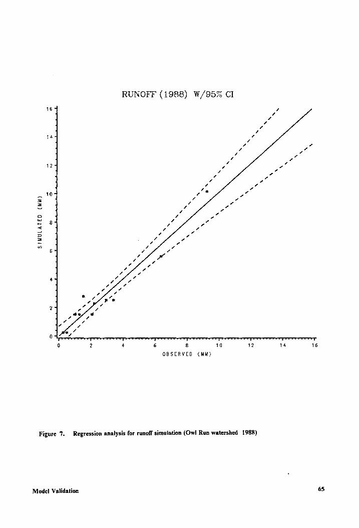
RUNOFF (1988) W/95% Cl

14

eg

kg ghee

—_

bo jes

—_ So

fh eer repealing

Bree

t cr

ea

ann -

abct

aee

fienecrilberee al

SIMULATED

(MM)

£0 rn

Boehner

len eel

0 2 4 6 8 10 12 14 16

OBSERVED (MM)

Figure 7. Regression analysis for runoff simulation (Owl Run watershed 1988)

Model Validation 65

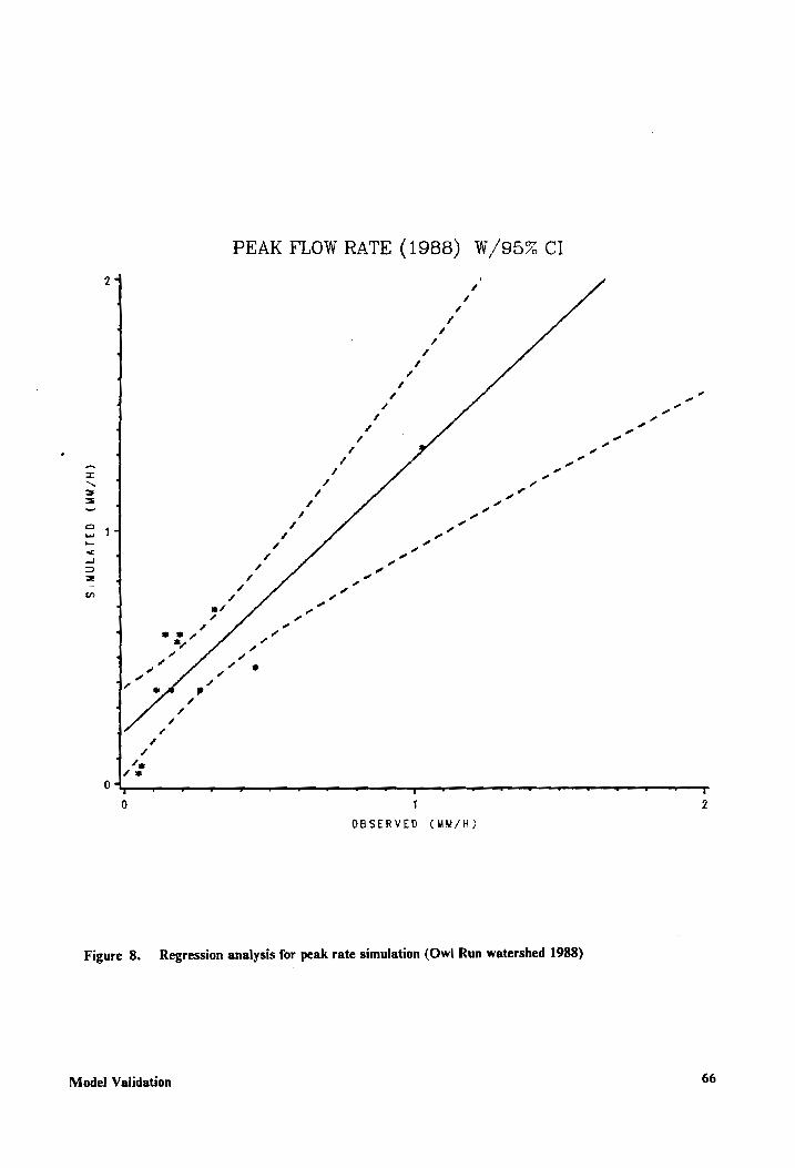
PEAK FLOW RATE (1988) W/95% CI

SiMULATED

(MM/H)

T ? 7 ¥ 7 r r —T 7 ¥ T T — T 7

9 1

OBSERVED (MM/H)

Figure 8. Regression analysis for peak rate simulation (Owl Run watershed 1988)

Model Validation 66

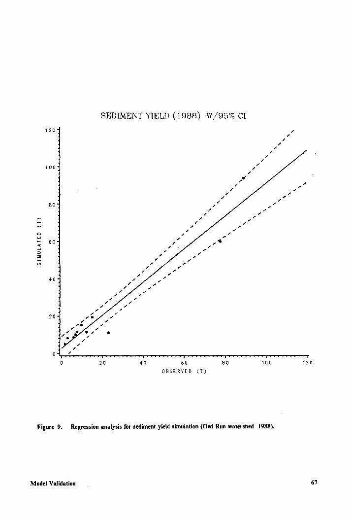
SEDIMENT YIELD (1988) W/95% Cl

120

100

BO

a WwW)

—- 60 < a

>

=

“

490

20

0 at ny] 0 20 40 60 80 100 120

OBSERVED (7)

Figure 9. Regression analysis for sediment yield simulation (Owl Run watershed 1988).

Model Validation 67

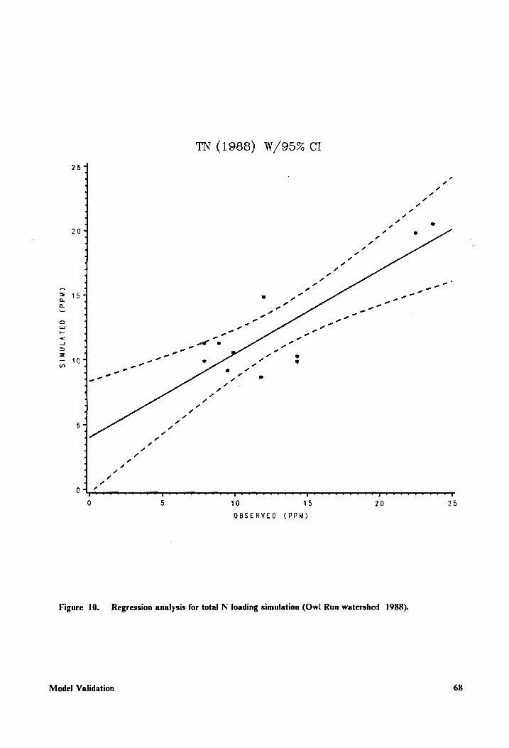
TN (1988) W/95% CI

nN on

ad.

20

15

10

SIMULATED

(PPM)

eB

ee Beh eee eee

eefienn

cl

fine

dhe

velhinerfientieenDenrdieafiedtinaiasderfianBat

haf p 2 ¢ £ g 2 2 g

Lendl B

t

Eel

TE ene “.”.CSFtC eter eel mreeelheeeeeee eee rele heehee cS reece T

0 5 10 15 20 25

OBSERVED (PPM)

Figure 10. Regression analysis for total N loading simulation (Owl Run watershed 1988).

Model Validation 68

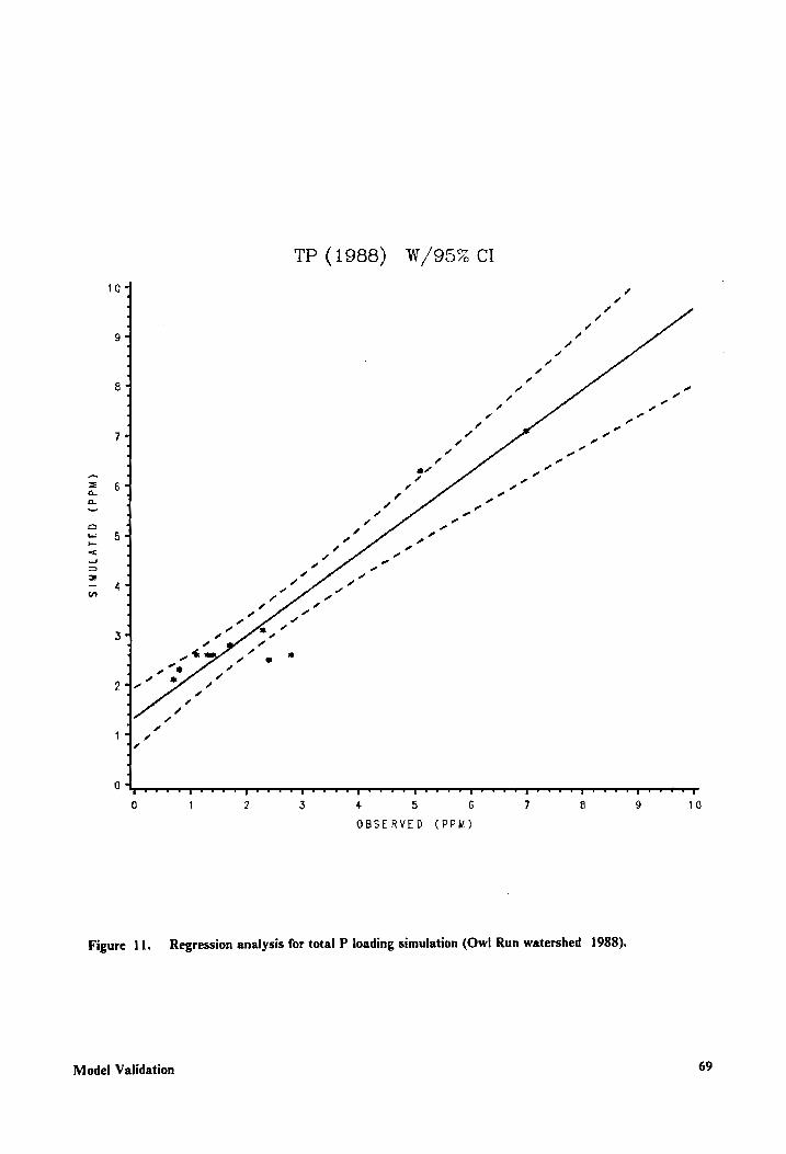
TP (1988) W/95% CI

wn ~

oO

Pacer

Re

Bhee

Bar

n fe

re S

acer

Ser

cann

Bhne

eeSb

ree

fhe tear,

MicedeeeerBiee Beer B

rees H

ana

Hb or

ecBi

eeer

rBen

eica

rne

SIMULATED

(PPM)

on

Be

lh ee

l ee

e Beeld

Gt

Pha cen

fiemne

creche

he

a he een

erred

enie

emet

oerr

dl

_s

er

a a

a So

[ee ee ee es ee ee ee ee ee ee ee ee ek ee ee ee

0 1 2 3 4 5 6 7 8 9 10

OBSERVED (PPM)

Figure 11. Regression analysis for total P loading simulation (Ow! Run watershed 1988).

Model Validation 69

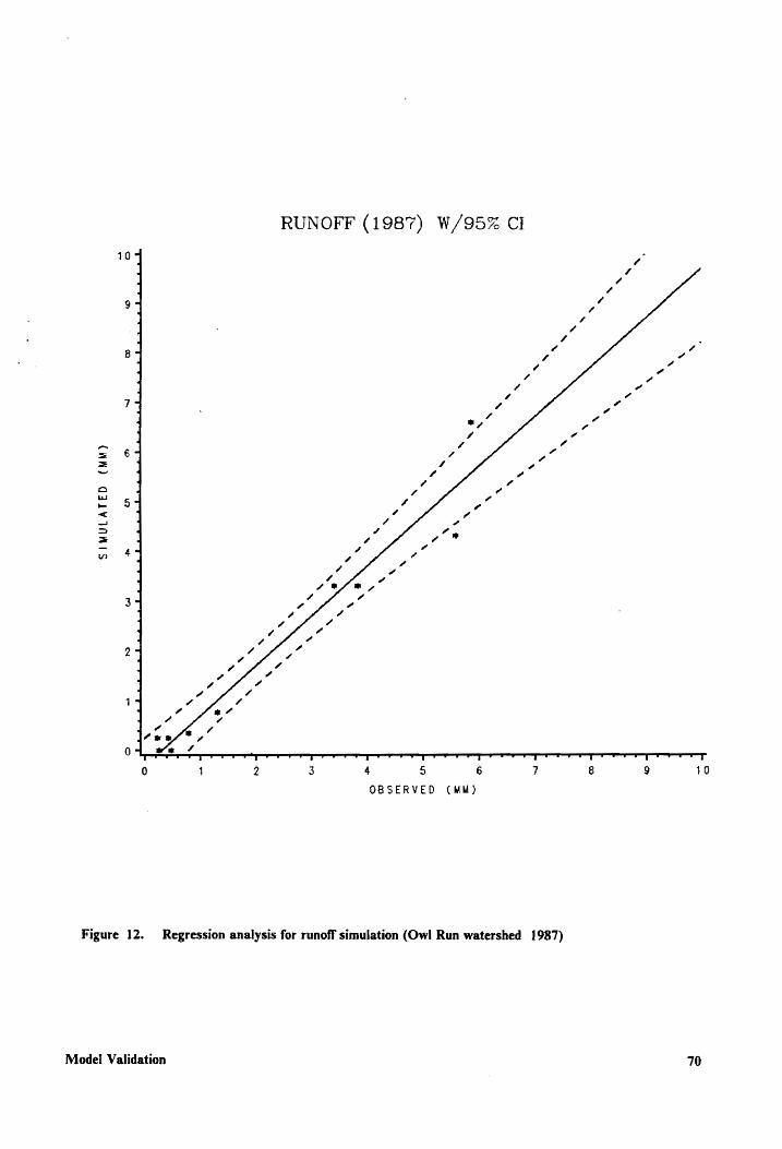
RUNOFF (1987) W/95% Cl

eB aee

e Be

a cael ere Beef

he

een

ree Beene

ne ee

e en

lere

edie

e fear

he

SIMULATED

(MM)

on

DoD eee

aa er

rr ee

l ea

eee

en

acelin cl areca

eT. CUP S:sCOrP dr? ee rhe hrm re eee

0 j 2 3 4 5 6 7 8 9 10

OBSERVED (MM)

Figure 12. Regression analysis for runoff simulation (Owl Run watershed 1987)

Model Validation 70

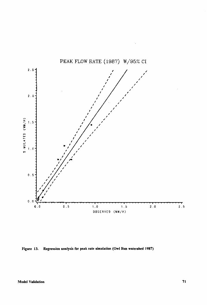
PEAK FLOW RATE (1987) W/95% CI

SIMULATED

(MM/H)

gett

a

Boe Be

cenB

iere

leee

nfne

rBne

feedicndl

oS oO

scal

lina

cvar

e Si

ndh

OBSERVED (MM/H)

Figure 13. Regression analysis for peak rate simulation (Ow! Run watershed 1987)

Model Validation 71

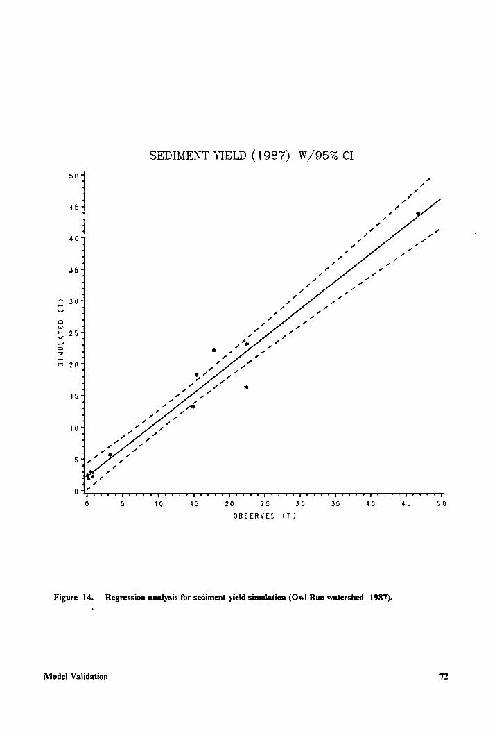
SEDIMENT YIELD (1987) W/95% Cl 50 4

454

40

BeBe

nf eeereent

el,

al

on |

Bnfen

30

25

SIMULATED

(T)

20

15

10

pet kt

eg nN

Reefer

eee

Bie Be

r fen

eel er

rand

s Jin

cadinsienBaxeabiemalieredees

ts, T”.”.':S”'~YSvrr’” ree ee hm eee

0 5 10 15 20 25 30 35 40 45 50

OBSERVED (T)

Tr .”" ' | FY ' | YT TY OT

Figure 14. Regression analysis for sediment yield simulation (Owl Run watershed 1987). .

Model Validation 72

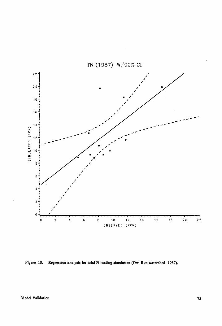
TN (1987) W/90% CI

20

16

Be

Bieclleeeefi

en

Bee

cerB

beee

eer

eee

eect

cB

ieee

eh pec

fien

enli

eren

fice

nfie

en

_

»

—>

bh

a on

a or a

a

ee e

e

=

oS

SIMULATED

(PPM)

©

Meee

Bae afr

rT

0 2 4 6 8 10 12 14 16 18 20 22

OBSERVED (PPM)

Figure 15. Regression analysis for total N loading simulation (Owl Run watershed 1987).

Model Validation 73

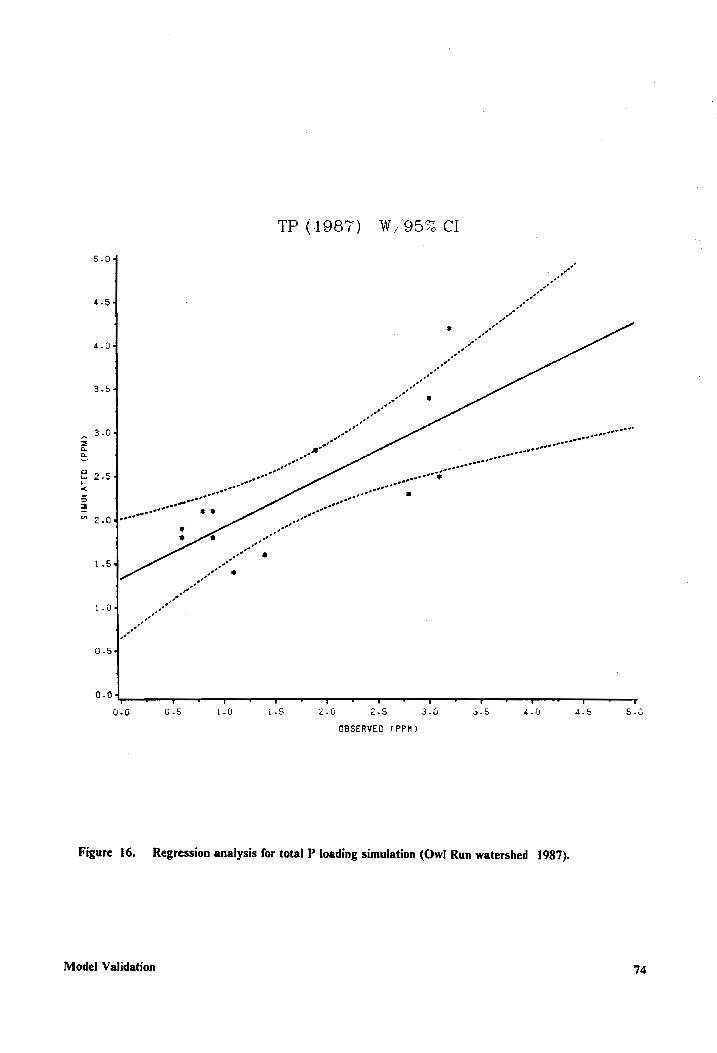
TP (1987) W/95% CI

SIMULATED

(PPM)

OBSERVED I PPH)

Figure 16. Regression analysis for total P loading simulation (Ow! Run watershed 1987).

Model Validation

74

Annualization procedure

To evaluate the effectiveness of various BMPs on downstream water quality, representative

storms, their magnitude and intensity, and their probability of occurrences need to be known, so

that the contributions of these storms to the average annual runoff, sediment yield, and chemical

loadings to downstream water bodies can be estimated. A big storm event may cause large amount

of pollutant losses in runoff, but its contribution to the average annual total loadings may not be

significant because of its low frequency of occurrence. Whereas relatively small events may cause

significant contributions because of their high frequency of occurrences [Koelliker and Humbert,

1989]. Therefore, individual storm events can not be used directly to evaluate long-term system

response. An annualization procedure is necessary to convert simulation results from event-based

water quality models for evaluating the long-term impacts of BMPs. Figure 24 shows comparison

of simulated and observed (from the 3-year data) distribution of contribution to runoff volume.

The comparisons provided by both of the table (Table 13) and the figure (Figure 24) further vali-

dated the parameters used in this study.

The annualization procedure explained in this section includes frequency analysis of rainfall

amounts and corresponding rainfall erosion indices (EI values in USLE), selection of representative

events based on the frequency analysis, sumulation, and summarization of these events.

Annualization procedure 75

Frequency analysis

As discussed in the last chapter, “primary events” (storm events with 24 hour rainfall amount

being equal to or greater than 7 mm in depth) may cause measurable runoff, sediment yield, and

chemical loadings. The data used in the frequency analysis for rainfall amount include a three-year

period of primary events, collected from Owl Run watershed during 1987 to 1989. In the

annualization procedure, storm events with all probabilities or return periods are required to sum-

marize contributions of different storms to annual pollutant loadings. Therefore, the data collected

from Owl Run watershed is too short to make a reliable frequency analysis, especially when ex-

trapolation is needed to determine the probability of occurrences of extremely large events [Linsley,

1988}. For this reason, results of a rainfall frequency analysis from a nearby station located in

Culpeper County, Virginia were used to extend the short record [Shanholtz and Lillard, 1973]. The

assumption made here is that the Owl Run watershed has similar meteorological conditions as

those of Culpeper county. The Culpeper series contains a ten-year period of record. This series was

mainly used for events with return periods of longer than two years.

The erosivity index of a storm event, EI, is calculated using the equation [Foster, G.R., et al.,

1981]:

n

El=1) (0.119 + 0.0873 log; o(i))D; (19) j=]

Where n is the number of time segments into which a storm is divided; I is the maximum 30-minute

rainfall intensity in mm/hr; i; is the intensity during the jth tume segment in mm/hr; and D, 1s the

depth of rainfall for the jth increment of the storm hyetograph. Frequency analysis for EI values

were also performed using the three-year data collected from Owl Run watershed. A 22-year rainfall

record for Richmond, Virginia [Wischmeier and Smith, 1978] was used to calculate EI values as-

sociated with larger events. The relationship between the probability of occurrence and return pe-

riod can be written as [Chow, 1964]:


P =—_— (20)

where P is the probability of occurrences of primary events being greater than or equal to certain

value; m is the average number of the primary events during a year, or the annual frequency of

occurrence; and T is the return period in years.

In frequency analysis of hydrologic data, theoretical curve-fitting is needed to interpret the past

record of hydrologic events in terms of future probability of occurrences. Theoretical frequency

distributions extensively used in rainfall frequency studies include Pearson type-I and type-II dis-

tributions [Pearson, 1930; Foster, 1924], Type-I extreme distribution [Gumbel, 1941; Chow, 1953],

and lognormal distribution [Chow, 1955].

Log-normal frequency distribution functions are found to be well fitted with the recorded

hydrological data [Chow, 1955]. A log-normal distribution is a transformed normal distribution in

which the variable is replaced by its logarithmic value. The probability density function of the dis-

tribution is

1 _(y—Hyy eo,./2n 205

P(x) = (21)

where x is the variable (rainfall amount or EI value); y = In x is normally distributed, with py and

oy being the mean and standard deviation of y. While the statistical parameters for the variable x,

including mean, coefficient of variation and coefficient of skewness (u, C, and C,), can be evaluated

by the complicated theoretical equations derived by Chow [1954], simplified procedures are widely

used in the engineering field of applied hydrology. This is because of the errors involved in the data

collection and enlarged by the calculation of higher power orders in the sophisticated equations.

One of the simplified procedures is based on the trial and error method. The statistical parameter

mean, py, is represented by the arithmetical mean of the recorded data x; the initial value of the co-

efficient of variation C, can be the calculated by using the standard deviation divided by the mean

value of x. The coefficient of skewness, C,, was evaluated by assigning an initial value, say 3C, or


2C,, and using curve fitting. The probabilities of the variable are calculated by using the table pro-

vided by Chow [1964].

In this study, a log-normal distribution function with mean, xX = 18mm, and coefficient of

variations, C, = 0.8, was found to be a good fitted theoretical curve for rainfall amounts. Another

log-normal frequency distribution function with mean, E] =51.7 MJ.mm/ha/hr, and C, = 1.7, was

fitted to the rainfall erosion index data. The results of the two frequency analysis for rainfall

amounts and EI values are shown in Figures 17 and 18, separately.

Selection of representative events

In order to estimate the average annual values from single storm simulations, a series of repre-

sentative storm events should be selected for use in the annualization simulation. The assumption

made in the annualization procedure is that each storm contributes to a portion of the average an-

nual amount based on its frequency of occurrence [Koelliker and Humbert, 1989]. A representative

storm to be used for AGNPS simulation is characterized by an amount of rainfall and an EI value.

A series of eleven different storms were selected with occurrence probabilities ranging from

0.0005 [return period, T, of 50 years, equation (20)] to 0.5 (return period, T, of 0.05 years). The

rainfall and EI frequency curves were divided into eleven frequency intervals intervals such that the

whole probability region (between 0 and 1) was represented (table 11). These eleven intervals on

each of the curves were also selected such that the differences in the magnitudes of neighboring

representative storms were not very large, in order to reduce the errors involved in the

descretization of continuous variables. The more representative storms selected, the more accurate

simulation results can be expected. The average rainfall amount and EI value on each of the eleven

intervals were used in the AGNPS simulations as the two characteristics of each representative

storm event corresponding to that probability interval. For example, the two values for the third


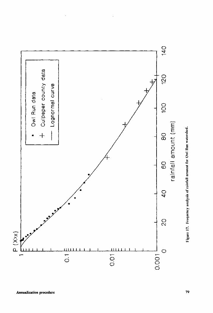
“poyssazem UNY

[MO 40J

JUnOW

|Ejures yo

siskjcue ADuanbaa,|

“Lf 94Nsty

(Lull) JUNOWP

|BsUuses

Orl OdL

OOL 08

O09 OV

O07? O

-+ 7

T 7

- 1

LOO'O

7 4100

- i A LO

BAIND jewwsOUBOT ——

2

Bye

Ayunod JededingQ

+ -

elep UNH

IMO 1 4

|

79 Annualization procedure

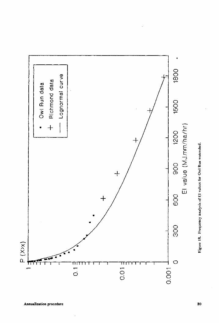
7°

(AU/BYU/WLUP

YY) @N|BA

|3

*PAYSAIIEM UNY

IMO JOJ

sanNgeA J]

JO SisApeue

Louanbaay “gy

aansiy

OO06L OOGL

OO0dL O06

009 OO0&

q

I

BAIND jewWwsoUBC TD

~__

Byep puowyojiy

Byep UNY

IMO os

i i

| +

q ard bt J Oe |

|00'O

LO'O

L'O

80 Annualization procedure

representative event (i = 3) required by AGNPS input were R; = 28.4 mm and El; = 78

MJ.mm/ha/hr. R; is the average value of rainfall amount on the 3rd interval of the frequency curve

in Figure 17 (table 11); EI; is the average value of erosion index on the 3rd interval of the EI fre-

quency curve in Figure 18 (table 11); both of the two values have the same probability of occur-

rence, P; = 0.15 (return period T = 0.1667 years for annual occurrence frequency P3,m = 6

times), which is used in weighing the annual contributions of this representative event.

Simulation and summarization

With the representative storm events selected following the procedures described in the last sec-

tion, direct AGNPS simulations were made and summarized to find the average annual results.

Let n be the number of probability intervals into which the whole probability region is divided

(or the number of representative storm events to be used in the annualization procedure), the an-

nual contribution of all representative storms can be expressed as:

n

Ct=m ) f(R;, EI)P; (22) i=1

where Ct is the annualized simulation result contributed by all the representative storms; R; and

EJ, are rainfall amount and erosion index of the i th representative storm event, 1= 1,2, ... n (n= 11

in this study); m is the average number of primary storms occurring during a year, or the annual

frequency of occurrence of all possible events; P, is the interval probability corresponding to the

i th representative storm; and f(Rj, Eli) is the AGNPS simulation result for each storm with input

of Rj and E];. Ct could be runoff, sediment yield, or any of the chemical loadings simulated by

AGNPS. Since a representative storm may occur during any season of the year, it should be sim-

ulated for each season and summarized as:


k

f(R;, El) = )f(R;, El, Para)Ps, (23) j=l

where k is the number of seasons used for a year (k = 2 in this study, for dormant and growing

seasons); Para, denotes all the parameters used for the j th season’s simulation such as CN, C factors

in USLE, etc.; and f,(Ri, Eli, Para) is the direct simulation result of the i th representative event

for the } th season simulation, it could be runoff, sediment yield, or nutrient loadings. The

f,(Ri, El;, Paraj) values corresponding to runoff, sediment yield, and chemical loadings for the two

seasons are listed in Table 7 and table 8. Ps, is the percentage of the ith representative storm

occurring during the j th season. Values of Ps, are also listed in Tables 11 and 12. The probability

of a storm event occurring during different seasons is not evenly distributed. Generally, small events

occur in dormant season more than in growing season, while extremely large events occur most of

the time during growing season. The probabilities of the storm events occurring during the two

seasons were calculated in percentages using the three-year period data from Owl Run watershed.

These percentages are listed in table 1] and table 12.

The probability of the representative event P;, in equation (22); annual frequency of occurrence,

mP,, in equation(22); the average rainfall amount, R;; and the rainfall erosion index value, El;,

corresponding to each frequency interval, i, were taken from the two frequency curves in Figures

17 and 18. A summary of these values are also listed in Tables 11 and 12.

Runoff, sediment yield, total nitrogen loading, total phosphorus loading, and total chemical

oxygen demand loading, were simulated to estimate the contributions of storms with different

magnitudes and frequencies. The outputs from each simulation run f,(Rj, El,, Para), multiplied

by the corresponding occurrence frequency (mPj), and weighted by the seasonal percentage (Pj),

give the annual contributions made by each representative storm. Figures 20 through 23 show the

contributions of every representative storm to the annual average (in percentage) runoff, sediment

yield, total nitrogen loading, and total phosphorus loading, corresponding to the rainfall amount

and the annual occurrence frequency of the event.


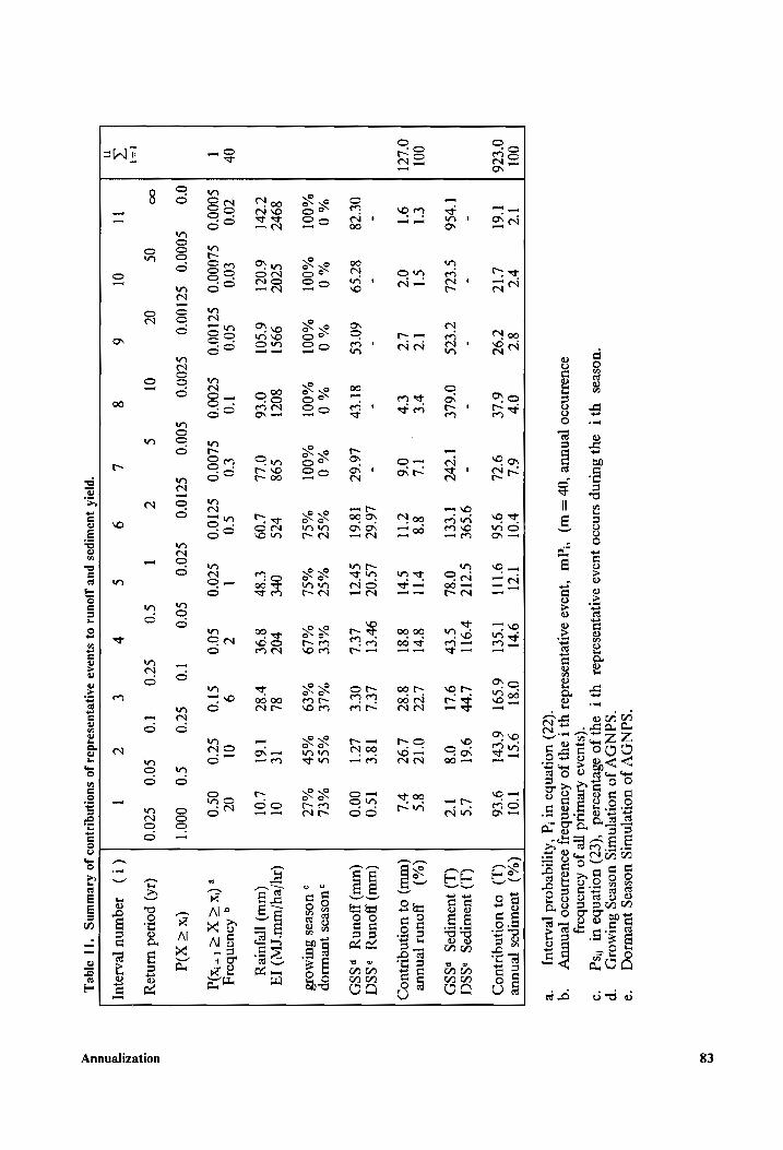
‘SdNOV

jo Uoyenung

vosesg yuRWIOg

= °3

“SdNDV

JO UOe[NUNIS

UOseaS SUIMOIDH

‘uoseas Y1T

94} SuUUNp

sind00 ydAd

SATFEJUASOIdSI YT

yy Jo

odejusoied ‘(¢7)

UoTenba ut

"sg

See!

*(syusao Areurtid

Tye Jo

Aousnboyy s9u01INd90

JenuUR ‘Op

= W)

“qui ‘jUdA9

dATVEJUDSOIda|I Y}

1 OY} JO

Aduanbay sousuNs90

Jenuuy =°q

‘(@Z) uonenbs

ut 'g

‘AyqIqeqoid yealouy—s*B

001 0'€26

001 O'LCI

—_

=A o -

Ve V6l

ps6

el 91

0¢°C8

% 0

“001

897 CCI

c0°0 $000°0

00

oo

I

¥'C Lic

87°S9

“% 0

“001

$202 6 0c!

t0°0 ¢L000°0

8

o9C

OLS

Ve Lt

60°¢S

% 0

"001

99ST 6S0I

$00 $c100°0

$0000 scl000

0S

OI

0c

OV OLE

0°6Lt

vt tv

3 % 0

001

8021 0'¢6

V0 $c00'°0

¢c00°0

OI

6L v'0I

ICL 9°S6

- 9°99¢

Vere eel

UL 8°8

0°6 cl

- L6'6¢

L66C =:

1861

% 0

“SC “001

“SL

$98 bes

OLL £09

€°0 $0

$4000 $cI00

S000 Sszr00

¢ Cc

L 9

Vel OTT

CCl? OSL

vit Stl

LS‘0¢ svcl

“ST "SL

Ope t 8p

I $700

$c0'0

S

orl sel

roll o'tV

I a |

8°81

9v'Cl LEL

“ott “%L9

v0C BOL

C $00

$00

$0

v

O8l 9ST

6S91 6th

Ler 96l

OLI 08

Le

O1@ 88C

=

LL 92

LeL 18

ore Lol

“LE %SS

9

VSP

8L It

vse =i

6l

9 01

STO Sce0

TO sco

$0

$c0 TO

8 $00

t c

TO! 9°€6

L's Ve

8°¢ VL

1S°0 00°0

“oth “LT

ol LO!

0c 0S°0 000°T

$c0'0

I (%) yUOUNpes

yenuue

(L) 01

vornquyu0D

(L) wuauNpss

»SSci (1)

yuauNpag pSSO

(%) jounl

fenuue (mu)

0} UONNQUyUO,

(um) founy

»SSd (uu)

youny pSso

9 UOseas JURUTIOp

> UOSRaS SUIMOIS

(zy/ey/urur fy) 14

(urur) jfefute yy

q Aouonbol]

o(X< X=)

(X < X)d

(14) powod

winjoy

(1) soquinu

yeAlsjuy]

“pjard quDWIpPOS

PUB YOUN

0} SjUdAd

JAIVBJUISaId94 Jo

SUOINGIIQUOD Jo

AyEWWNG

*]] 31921

83 Annualization

Relationship between rainfall amount and erosion index

Rainfall amount and its corresponding EI value are required by the AGNPS model as inputs for

each individual storm event simulation. Storms with same magnitude of rainfall amount may result

in a different EI value because of both temporal and spatial variations in rainfall intensity. There-

fore, a frequency analysis of two dimensional distribution, or determination of their joint distrib-

ution, may be ideal in selecting the two values as the model input. In this study a simplified

procedure was used by selecting rainfall amounts and EI values from the two individually-analyzed

frequency curves. In doing this, it was assumed that events with same amount of rainfall have same

EI value. For example, the rainfall amount taken from the rainfall frequency curve in Figure 17

between 0.1>P2> 0.05 was averaged as 36.83 mm on interval number 4; the corresponding EI

value was taken from EI frequency curve in Figure 18, with average value of 204 MJ.mm/ha/hr

on the same probability interval. The probability of this representative event occurring within this

interval is 0.1 — 0.05 = 0.05, which is used as the weight [P, in equation (22)] in summarizing the

simulation results.

The rainfall amounts recorded in Owl Run watershed during the 3-year period are plotted against

their EI values in Figure 19. Rainfall amounts and EI values of representative events taken from

the two frequency curves are also plotted on the same figure. The line joining the points of repre-

sentative events passes through the scattered recorded data points. This line represents the averaged

EI values for each representative rainfall amount. As mentioned above, only the representative

storm events were used in the simulation.


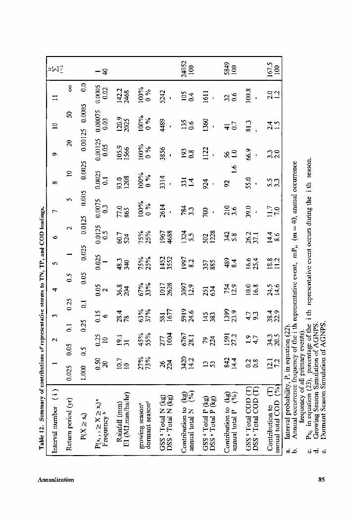
"SdNDOV JO

UoHe[NuNs Uoseag

JUeULIOg «=

‘9 "SdNDV

Jo UonR[NUNS

UOseas SUIMOID

“UOSEdS Y}T

34} BULINP

sINDIO WUSAS

oATJEUDSIIdaI YI

OY} JO

oseyUa.IOd ‘(¢z)

UoWenbs ut

"sg ‘(syuoaa

ATeurud ye

jo Asuonbay

99U91IN990 JenuUL

‘Hp =

WI) “Iqul

‘jUdAo sAtjREJMasoIder

Y} 1 oy}

Jo ADUaNbolj

sdudIINDIO Tenuuy

“q "(7Z)

uonenba ut

'g ‘Aypiqeqosd

yealojuy “eB ord

85

001 ZI

cl 07

Ce OL

9°8 (aan

orl 67

S02 ZL

(%) GOOD

[eI0} Jenuue

SLOT] 07

p72 €C€

cs Lil

rr 8°31

CPZ pss

€Pre ITI

(L) 0}

uornngimu0Z

- -

- -

- Ve

y'Sz 8°91

£6 LY

80 (L)

dOO FOL

» SSG 8001

C18 6°99

oss 0'6€

797 9°91

001 LY

61 Z0

(L) GOD

TROL p SSD

001 9°0

L0 O01

91 9°¢

gS p's

67I 62

Tle vl

(0%) q

yev0} Jenuue

6P8S 7

Iv 9¢

76 O1Z

Zre 68r

PSL 66€1

16SI 7br8

(34) 0}

UoTNqIUyUOZ

- -

- -

- 82Z1

C88 reg

€8&—s-w7Z €¢

(34) d

TRIOL » SSA

LI9T O9€T

2211 $76

OOL Z0S

LSC 1SZ

Srl 6L

€1 (84)

d IO.L

p SSO

001 r'0

9°0 80

rl ec

as 78

67 972

T8% Tl

(%) N

Jei0} fenuue

zsorz| =

SO Sel

£61 I€e

p8L p7f]

L661 L60C

616 L9L9

OPE (34)

0} uorNquUyUOZ

- -

- -

- 889p

~sse 879%

LLOT Yf00!

b7Z (34)

N PIOL

» SSA 7b7S

68rr 9S8E

PIC’ p19T

L961 = TSC

18S LLZ

97 (34)

N [230.1

p SSD

% 0)

% 0)

% 0

”% 0

% 0)

%ST MST

MEE MLE

MSS MEL

sUOSBas JURULIOP

*%001 %00l

%001 %O00l

%00l “SL

MSL LI

MO

Br

%*LZ Uoseas

SUIMOIE

89P7Z SZ0Z

99S 80ZI

698 b7S

Ore r0Z

8L I€

01 (ry /ey/uor f])

[4 Zr

6071 6'SOI

0'°€6 O'LL

L'09 € 8p

8°9€ p8t

l6l LO!

(ur) yeyuTey

Or |

zo0 £0'0

c0'0 10

£0 C0

I Z

9 OI

02 q Aouanbarj

1 |

s0000 SZ2O00°;0

SzI00;0 sz00;0

$4000 SzI00

S200 ¢0'0

S10 Szo

oso eX

ZK

<I tRY

00 s0000

SzI00';0 sSz00o0

sooo Sszi0o0

sz00 s00

SZ'0 SO

0007 (x

= X)d

oo 0s

02 OI

¢ Zz

I S70

soo Sz0'0

(14) poued

uinyay J=!

< Il

Ol 6

8 L

9 ¢

P €

Z I

(1) Joquinu

pearsyuy

*‘sBuipeo] GOD

put ‘dL

‘NLL 0}

Swi40j3s aatyejuasaidas

Jo suonngiajuos

jo ArewuNS

‘Z| 3qGe 1

Annualization

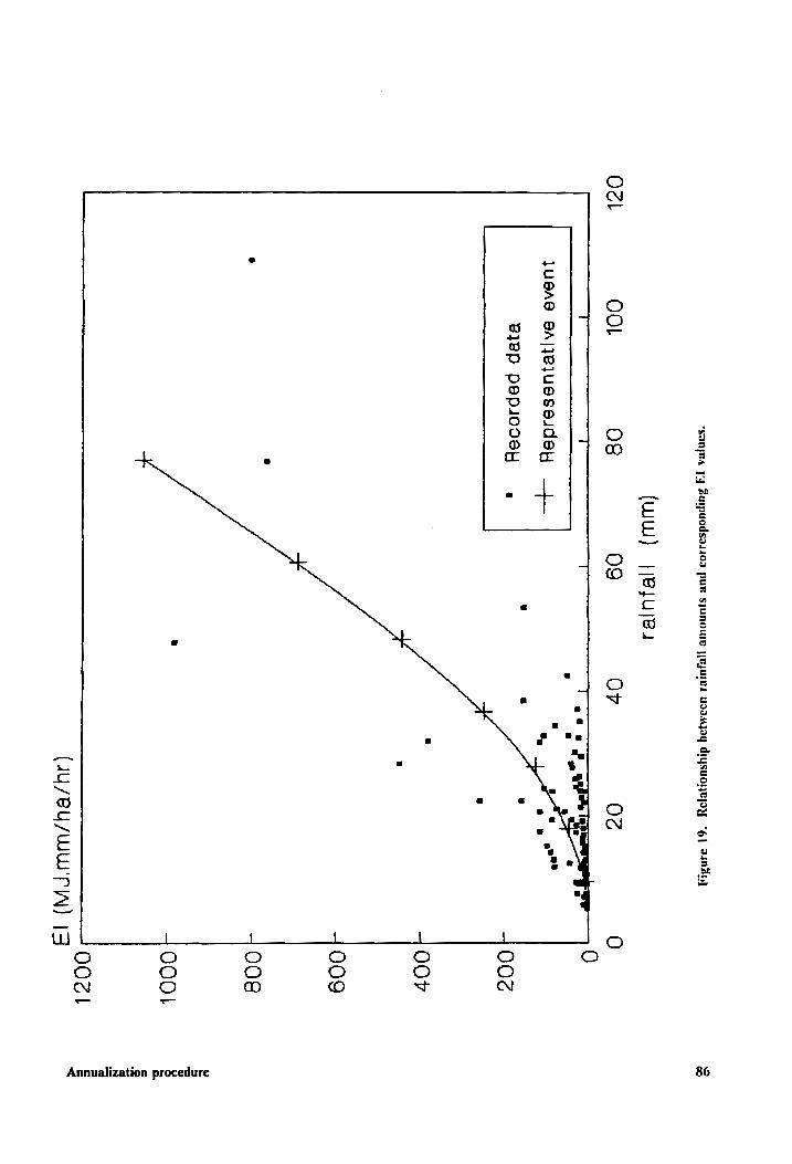
OdlL

"sanyea [A

Suipuodsass0d pue

syunowe jpejures

udaMjaq diysuontpay

“6] 34n814

(Ww) ||/Bsuses

OOL O&

Og OV

O¢ |

{ {

T eee

Ww

JUBAG BA]E]UESe1d8yY

1

"ae aoe"

Blep pepsooey

Sy .

. .

(ay/BY/WW'PW) 13

00d

OOF

O09

008

Q001

OO07d1



As described in the previous chapter, AGNPS parameters related to landuse and surface cover

conditions were prepared for different seasons; parameters related to topography and soils were

prepared for the whole year; antecedent soil moisture conditions for determination of curve num-

bers was assumed to be condition-II as used in the validation of the model. The simulation results

obtained from AGNPS using the annualization procedure were compared with the observed data

from the Owl Run watershed [Mostaghimi, et al., 1989]. Table 13 shows the average annual sim-

ulation results compared with the data collected during each individual year and the average of the

three years from the Owl Run watershed. Distributions of contributions to annual runoff volume

were also compared between the simulated results and the 3-year observed data (Figure 24). As

shown in Figure 24, the observed and simulated distribution agree reasonably well and indicate the

validity of the distribution used in the annualization procedure.

Generally, the results compared favorably with the observed data. The annual average sediment

yield, and total nitrogen loadings were slightly overestimated, while the total phosphorus loadings

were underestimated. One possible reason for the discrepancy between the simulated and observed

value is that the extreme values of rainfall erosion index data from Richmond, Virginia, was used

in the EI] frequency analysis for Owl Run watershed. The rainfall intensity in Richmond, Virginia,

is generally larger than that in Fauquier County, Virginia [Herschfield, 1961]. In addition,

fertilization levels and fertilizer availability factors are required by AGNPS as input parameters for

individual events. This is a major weakness of event-based models, since the parameters have to

be prepared for the entire season as average conditions in long-term simulations, which is more or

less subjective. The data reported by Mostaghimi et. al. [1989] indicate that high concentrations

of nitrogen and phosphorus were detected shortly after the chemical applications on the field. This

phenomenon is difficult to simulate by using representative storms. A great amount of variability

in the observed data was found among individual years. It should be noted that the annual predic-

tion values made AGNPS are well within the ranges represented by the recorded data from the Owl


Run watershed for the three years of the study. Once sufficient amount of data is collected, such

discrepancies can be minimized by comparing the simulation results with the observed average an-

nual results.

From the results displayed in Figures 20 through 23, it can be noted that, events with annual

occurrence frequencies of 6 to 10 times/year (return periods of 0.1667 to 0.1 years), are responsible

for majority of the annual pollutant loadings. Therefore, more attentions should be made in de-

signing BMPs sensitive to these small events.

The annualization procedure provides a basis for evaluating long-term effectiveness of various

BMPs. For identification of critical areas within a watershed, the concept of perennial effects should

still be considered. The critical areas in this study were identified by using the annualization pro-

cedure explained in this section. A computer program was developed to summarize the AGNPS’

output files with different representative storm’s input on a cell basis. Comparisons of annualized

critical areas identified for the circumstances before and after a BMP implementation scenario are

discussed in the next chapter.


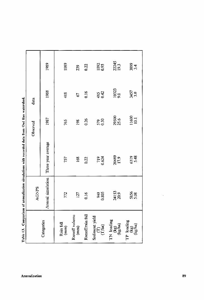
re Oe

LOT gr's

80°S (ey/3¥)

668E LOPE

OO9TT 61¢9

98S (34)

suipeo] dL

C61 06

9°SZ 6 LI

6°02 (ey/3y)

SPTCZ €ZC01

00S6Z 68902

€S1PZ (34)

suIpeo] NLL

660 Zr’

0s°0 $790

6080 (eq/1)

7601 C8P

6LS 614

Or6 (1)

pists yusuNpas

7Z'0 910

97°70 770

910 Trey

Ures/fyouny

6€7 L9

861 891

L71 (uray)

ounyjoA youny

6801 SIP

SOL LSL

CLL (urut)

[rey urey

6861 8861

L861 odesoae

Jeo sayy,

| UorEyNuNs jenuuy

salodoje-)

SdNDV

eyep

PeAresgg

“payssayem

UNY IMG

WO

BzPEpP papsooad

YPM SUOIZeINULIS

UOHeZYEnUUR yo

UOSIIedWIOZ “Cy

21qR

89 ization Annual

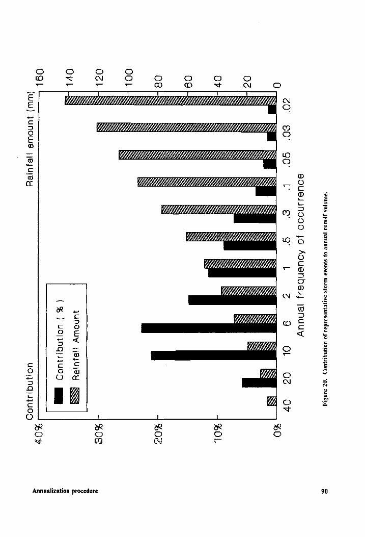
© © O

© st N © © © © O _ — — — 08) ©O <t N ©

E L111 OOOO

3 W000] & Aca)

= KITE]

& (TMQ

MIM QO

NX

AT

R

~ § TX Se 2 = TUN 25

c|/| EE Z\|6¢ ANN —

= \ =I! A A O O l l

eR ar aR HR xR © © © © oe) et aa) ay -


05

.03

02

i” 3

Annu

al

frequency

of occurrence

20

10

40 Figure

20.

Contribution

of re

pres

enta

tive

st

orm

even

ts

to annual

runo

ff vo

lume

.

90

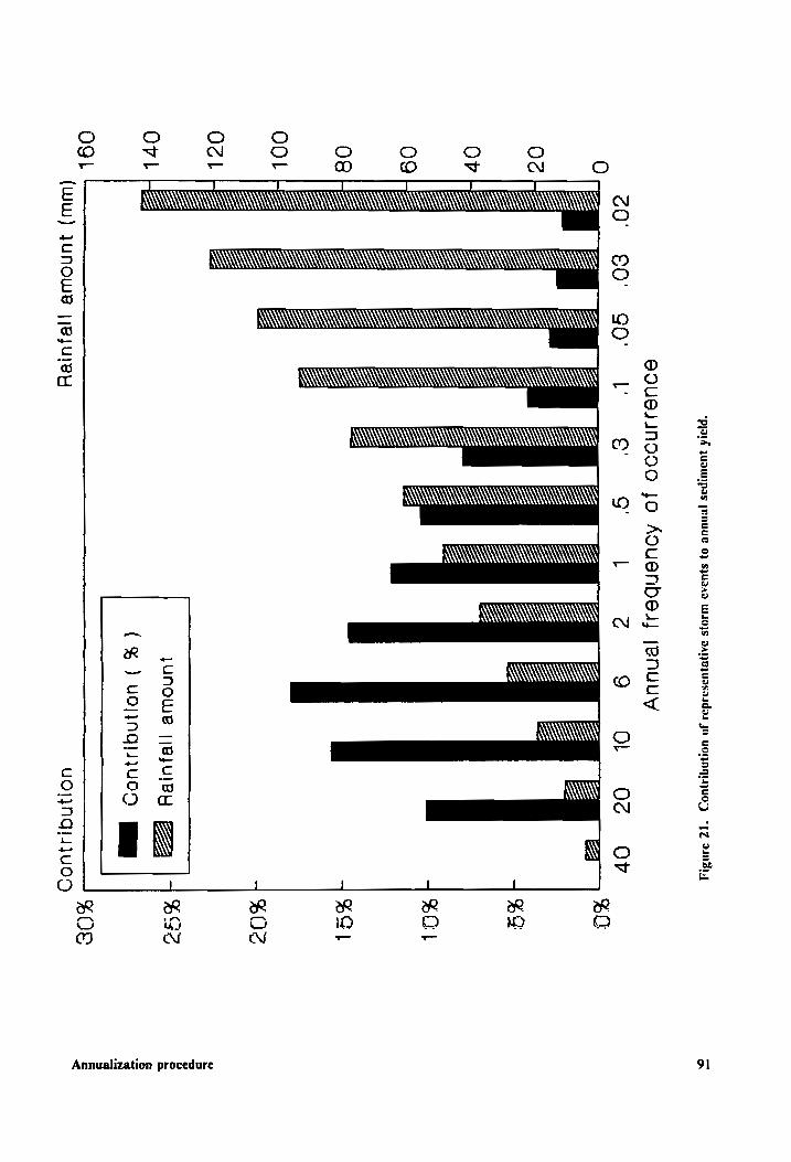
© © © O Ce) wt N © © © © O

- - - © oO a A Oo

E {III MMMM)

3 ITI) © e -

oO

= (III 2

& Wl 0 0"

MIM ©

NOOO

AI

WI) Rr ~ § A co c °o S €

2 = TO) o <-|| € © = SO AW a “ 5 BX Wo Oo ~t © ! __j _I I I

rend aR KR ae xR HR ran So ud Co WD O MD 2

Cc Ni a — —


Annual

frequency

of occurrence

Figu

re

21.

Cont

ribu

tion

of

re

pres

enta

tive

st

orm

events

to annual se

dime

nt

yiel

d.

91

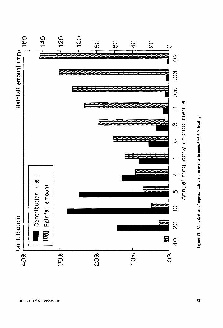
© O © O © a 9 N © © © O O — — —- — a cO wt N O

E (III IIo OO O©™®™©™ MM]

3 ITI M<™<™™ My] E

oO

= MII <€<©mk

& (III

MII

MMM]

_ IT « ro

~ § UI sé 2 = TT = @

c/| <¢ € EI(oé YS J

= \ =1/ HA x O O i i

eR on K oR aR Q Q Q Q QO st cy WN —


05

.03

02

i” 3

Annual

frequency

of occurrence

©

40

20

Figu

re

22.

Contribution

of re

pres

enta

tive

st

orm

even

ts

to annual

tota

l N

loading.

92

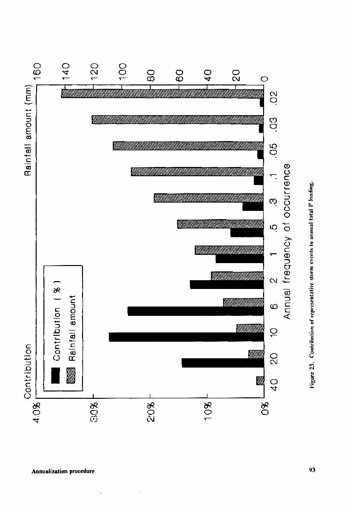
a

L.


© © © © Ce) —t N OQ © O © © _ — - — © oO t N OQ

E (IMO MK OOO OMOO™©XO™O©™<oyAY

3 WWW aa g e -

wo

= MII 9

& WTI _

LI «>

AU

II

_ I wR

~ § ANI S é 2 = ANKE

s|| § & . = 6 € WN O y

= BX Wie) Oo wt O { _4 _t

a Or aR oR oR O © O O Q =f ' iN —

Annu

al

frequency

of occurrence

Figu

re

23.

Contribution

of re

pres

enta

tive

st

orm

events

to annual

tota

l P

load

ing.

93

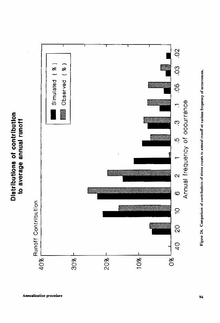
MME

Simu

late

d ( %)

Observed

( &}

LA

Distributions

of contribution

to average

annu

al

runoff

Runoff

Contribution

AUN

LK

AK

AY

AIIM

AW ovwyy'|\

AK

A

40%


30%

F

20%

10% F

O%

N ©

AY

03

08

20

10

AQ

Annu

al

frequency

of occurrence

Figure

24.

Comp

aris

on

of contributions

of st

orm

events

to annual

runoff

at va

riou

s fr

eque

ncy

of occurrences.

94

BMP simulation for Owl Run watershed

The purpose of this chapter is to evaluate the impacts of hypothetical implementation of BMPs

on surface water quality in Owl Run watershed using the AGNPS model along with the

annualization procedure. All the scenarios (currently intalled and proposed) were simulated using

the annualized version of the model. The cell size and the input parameters for the model were the

same as used in the model validation and the annualization sections.

The following seven BMP scenarios were simulated and their long term impacts on reducing

pollutant loadings are discussed in the following sections:

1. Present scenario (BMPs currently installed in the watershed);

2. No-till practice on critical areas;

3. CRP (Conservation resources program) on critical areas;

4. Installation of animal waste storage facilities;

5. No-till on critical areas plus animal waste facilities;

6. No-till on all agricultural land plus animal waste facilities;

7. All cropland converted to pastureland plus animal waste facilities.

BMP simulation for Owl Run watershed 95

Scenario description

Present scenario (Scenario No.1)

As part of the cost-share program implemented by the Virginia Department of Conservation and

Recreation, Division of Soil and Water Conservation (VDCR-DSWC), a combination of BMPs

were installed in the Owl Run watershed. The BMPs installed include no-till, strip cropping, CRP,

grassed waterways, animal waste storage structures, vegetative filter strips (VFS), and fencing. The

areas and locations of these practices are shown in figure 25.

As illustrated in figure 25, no-till was implemented on about 150 ha of corn, or 13 percent of the

entire watershed area. For no-till crop fields, the crops are planted in the previous crop residue with

minimum soil disturbance. This practice results in decrease in the curve numbers and C factors to

reduce surface runoff and soil erosion, and would increase the Manning’s n and surface condition

constant to increase the resistance of the land surface to the overland flow. The no-till practice also

increases the fertilizer availability factor, which has negative effects on improving water quality.

The strip cropping practice was implemented on about 50 ha of crop land within the watershed

(4.5 percent of the watershed in area). A stripcropping system refers to growing crops in a sys-

tematic arrangement of strips or bands across the general land slope to reduce water erosion and

nutrient losses [VDCR-DSWC, 1990]. Like no-till, this practice decreases the curve numbers and

C factors, increases the surface condition constant and Manning’s roughness coefficient, but does

not influence the fertilizer availability factor.

Conservation reserve program (CRP) requires that highly erodible cropland be retired for a pe-

riod of 10 years. While the “reforestation of erodible cropland and pastureland” is an eligible

Virginia state cost-share program, the CRP in Ow! Run watershed was implemented as converting

highly erodible lands (annual sediment erosion rate exceeding the tolerance limit, T) to grasslands.

This practice is enforced on about 12 ha area within the watershed. Cells on which CRP is imple-

mented are stmulated as hayland.


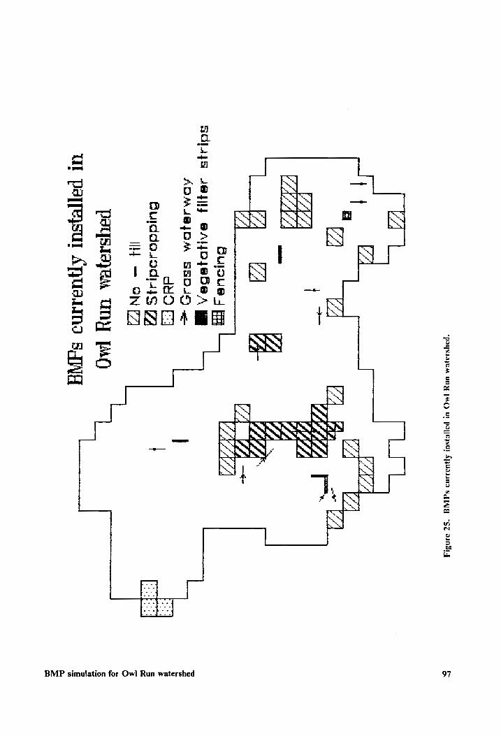
“payssayem UNY

IMG) Ul

Payeysul APUIIIND

SGING, "SZ

3403

r ri

ee

,

vot 4

’ cS

whores Fae

re

—

a 7

“ o

oF

/ a

doen Des

~

wn,

~,

RS Ny <

how

“e., —

97

‘f) Kh

— AMAL

T Gursue 4

FA LAL

VES

SC)45

184), eryoje6e,

mm

ADMIGIOM

BEDUS) we.

|

duo

£2] Buiddawodius

tt} =

ON EA

paysiayea UY

[Ag

Ul payeysul

APWALMI sq

BMP simulation for Owl Run watershed

A grassed waterway, or sod way is “a natural or constructed waterway, shaped or graded and

established in suitable vegetation, to safely convey water across areas of concentrated flow”

[VDCR-DSWC, 1990]. There are about 2.1 km of grassed waterways currently installed in the

watershed.

The Virginia agricultural BMP cost-share program [VDCR-DSWC, 1990] describes animal

waste control facilities as “a planned system designed to manage liquid and solid waste from areas

where livestock and poultry are concentrated to improve water quality by storing and spreading

waste at the proper time, rate and location”. The animal waste storage facilities installed near five

dairy cow feedlots and a hog lot in the watershed now have an annual storage capacity of 16810

tons, which is enough to handle the annual production of the livestock manure (17000 tons/year).

This allows the appropriate timing and rate of the manure application. Simulation of animal waste

facilities are accomplished by assigning appropriate values for fertilization levels and fertilizer

availability factors (reasonable application rate and timing).

Vegetative filter strips, or grass filter strips are defined in VDCR-DSWC [1990] as vegetative

buffers that are located along the banks of water courses to filter runoff, anchor soil particles and

protect banks against scour and erosion. About 1.2 km of grass filter strips are installed within the

watershed for nonpoint source pollutant contro! from about 29 ha of cropland. Cells where VFS

was installed were subdivided into subcells using the routine in the AGNPS version 3.51 or higher,

with the finest level at 12.5 m? (82 ft x 82 ft). Parameters related to grass were assigned to the areas

where VFS located as described later in this section.

A pond and some of the stream banks (about 1.8 km in length) are fenced to protect water

quality by reducing the direct manure loadings by animals. The Virginia agricultural BMP cost-

share program for fencing practice has the following requirements for qualification of application:

1. The fence is 20 feet away (minimum) from the stream; 2. There is adequate vegetation between

the stream and the water body to serve as an effective buffer to improve the water quality; 3. The

stream is fenced on both sides. Like the procedure used for the simulation of filter strips, cells

where fencing is applied need to be divided into subcells. The fine cells on the stream side of the

BMP simulation for Ow! Run watershed 98

fence are assigned parameters (of AGNPS input) for grass fields, and those on the other side of the

fence are given values of the parameters as for pastureland.

No-till practice on critical areas (Scenario No.2)

This scenario assumes that no-till practice be implemented on all the critical areas (high erodible

areas with annual sediment yield being greater than 22.4 tons/ha) identified by the AGNPS model

with the annualization procedure. The total critical area identified within the watershed was 68 ha.

in the watershed.

CRP on critical areas (Scenario No.3)

Like scenario no.2, the CRP practice is to be enforced on the critical areas to evaluate the im-

pacts of this scenario on improving water quality. As defined in the first scenario description in this

chapter, the conservation resource program requires that highly erodible croplands be retired for a

period of 10 years. The highly erodible lands (critical areas identified according to the annual

sediment yield) are to be replaced by grass land.

Animal waste storage facilities (Scenario No.4)

This option evaluates the net effects of pollutant reductions due to the installation of animal

waste storage structures for handling livestock manure applications. There were about 80 ha of field

in the watershed on which heavy rate of manure was applied before the installation of the animal

waste storage facilities. As mentioned above, the five dairy waste and one hog waste storage facilities

have enough capacity to handle the animal waste of 6 tons/day (total solids).

No-till on critical areas plus animal waste facilities (Scenario No.5)

While the no-till practice 1s implemented on the critical areas, the manure is managed to prevent

over-application and to provide appropriate timing of application on the agricultural fields. This

option simulates the cumulative effects of the two practices on water quality.


No-till on all agricultural land plus animal waste facilities (Scenario No.6)

The difference between this BMP scenario and scenario no.5 is that, instead of the critical areas,

the no-till practice is applied on all agricultural lands including no-till on pastureland and hayland.

The animal waste storage facilities play the same role as that of scenario no.4.

All cropland converted to pastureland plus animal waste facilities (Scenario No.7)

In this hypothetical scenario, all the cropland in the watershed is to be changed to pastureland

under the assumption that the capacity of the animal waste facilities is enough to treat the waste

from all the livestock in the watershed.

Simulation procedures for each of the BMPs

No-till

For the cells on which no-till is implemented, parameters including curve numbers (CN), C

factors, surface condition constant (SCC), and Manning’s roughness coefficients (n) were adjusted

from conventional conditions to appropriate values corresponding to the practice. A summary of

parameters used for simulating the no-till practice on cropland, pastureland, and hayland is given

in table 14 for both dormant and growing seasons. The sources from which these parameters were

estimated are the same as those used in the model validation procedure.


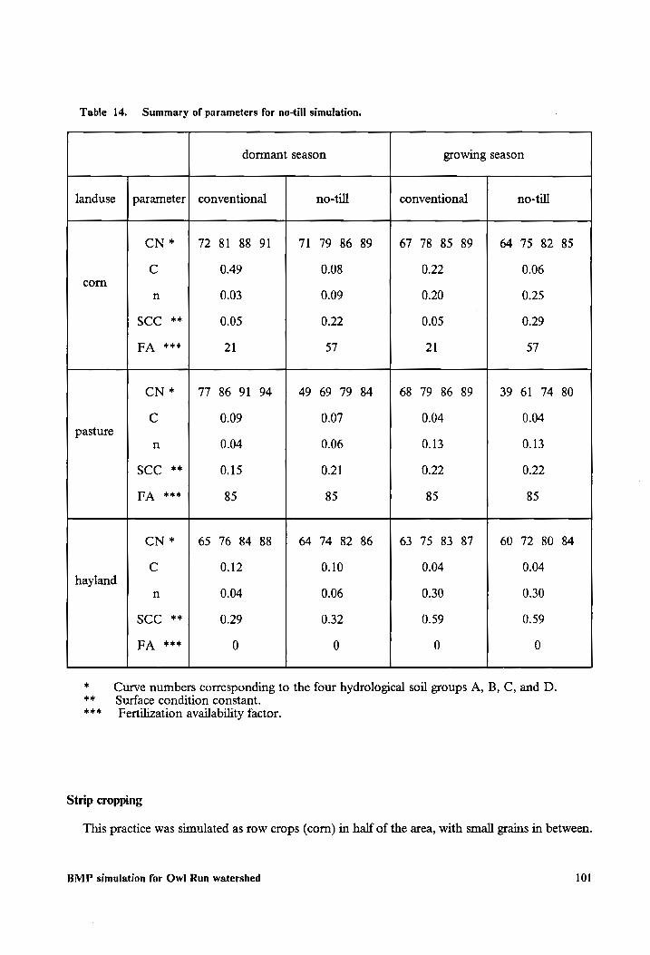
Table 14. Summary of parameters for no-till simulation.

dormant season growing season

landuse | parameter| conventional no-till conventional no-till

CN * | 72 81 88 91 71 79 86 89 67 78 85 89 64 75 82 85

C 0.49 0.08 0.22 0.06 corn

n 0.03 0.09 0.20 0.25

SCC ** 0.05 0.22 0.05 0.29

FA **# 21 57 21 57

CN * | 77 86 91 94 49 69 79 84 68 79 86 89 39 61 74 80

Cc 0.09 0.07 0.04 0.04 pasture

n 0.04 0.06 0.13 0.13

SCC ** 0.15 0.21 0.22 0.22

FA *** 85 85 85 85

CN * | 65 76 84 88 64 74 82 86 63 75 83 87 60 72 80 84

C 0.12 0.10 0.04 0.04 hayland

n 0.04 0.06 0.30 0.30

SCC ** 0.29 0.32 0.59 0.59

FA *** 0 0 0 0

*

** Surface condition constant. *k ok

Strip cropping

Fertilization availability factor.

Curve numbers corresponding to the four hydrological soil groups A, B, C, and D.

This practice was simulated as row crops (corn) in half of the area, with small grains in between.


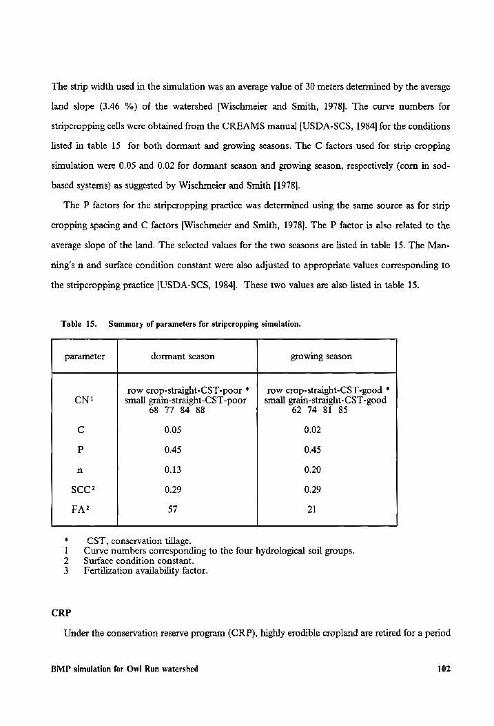
The strip width used in the simulation was an average value of 30 meters determined by the average

land slope (3.46 %) of the watershed [Wischmeier and Smith, 1978]. The curve numbers for

stripcropping cells were obtained from the CREAMS manual [USDA-SCS, 1984] for the conditions

listed in table 15 for both dormant and growing seasons. The C factors used for strip cropping

simulation were 0.05 and 0.02 for dormant season and growing season, respectively (corn in sod-

based systems) as suggested by Wischmeier and Smith [1978].

The P factors for the stripcropping practice was determined using the same source as for strip

cropping spacing and C factors [Wischmeier and Smith, 1978]. The P factor is also related to the

average slope of the land. The selected values for the two seasons are listed in table 15. The Man-

ning’s n and surface condition constant were also adjusted to appropriate values corresponding to

the stripcropping practice [USDA-SCS, 1984]. These two values are also listed in table 15.

Table 15. Summary of parameters for stripcropping simulation.

parameter dormant season growing season

row crop-straight-CST-poor * | row crop-straight-CST-good * CN! small grain-straight-CST-poor | small grain-straight-CST-good

68 77 84 88 62 74 81 85

C 0.05 0.02

0.45 0.45

n 0.13 0.20

SCC? 0.29 0.29

FA? 57 21

* CST, conservation tillage. 1 Curve numbers corresponding to the four hydrological soil groups. 2 Surface condition constant. 3 Fertilization availability factor.

CRP

Under the conservation reserve program (CRP), highly erodible cropland are retired for a period


of 10 years. The CRP is enforced on about 12 ha within the watershed. The retired croplands

maintain a condition of ungrazed pasture. AGNPS input parameters used for this simulation, CN,

C, SCC, and n were set to be the same as those of hayland as listed in table 14. The fertilization

level is assumed to be 0.

Grassed waterways

About 2.1 km of grassed waterways are currently installed in the watershed. At the locations

where grass waterways were installed, the value of Manning’s roughness coefficient for channelized

flow was adjusted from 0.048 to 0.060 [USDA-SCS, 1984]. It is assumed that gully sources do not

exist any more at these locations for post-BMP simulations.

Animal waste structures

Before the installation of animal waste storage facilities, the fertilization levels and availability

factors in AGNPS were chosen to be 2, and 100, respectively, as suggested by the AGNPS manual.

These values represent frequent applications of manure at high rate so that the pollutants contained

in the wastes are readily available to runoff. With the installation of the animal waste structures,

manure spreading is handled at proper time, rate and locations as required by the cost-sharing

program [VDCR - DSWC, 1990].

There are about 1000 dairy cows and 250 replacement heifers in the watershed [Mostaghimi, et

al., 1989]. Annual waste production of these animals is 17100 tons. The capacity of currently in-

stalled animal waste storage facilities is 16810 ton, which is enough to handle the manure applica-

tion at appropriate rate, timing and locations required by the cost-sharing program. The values of

fertilization level were reduced to 1 for the post-BMP simulation, and the fertilizer availability fac-

tors were reduced to regular values for different Janduses as listed in tables 14 and 15.

VFS

As indicated previously, for the AGNPS simulations performed in this study the basic cell size

was 4 ha (200 m x 200 m). At the locations where VFS and fencing are installed, the cells were


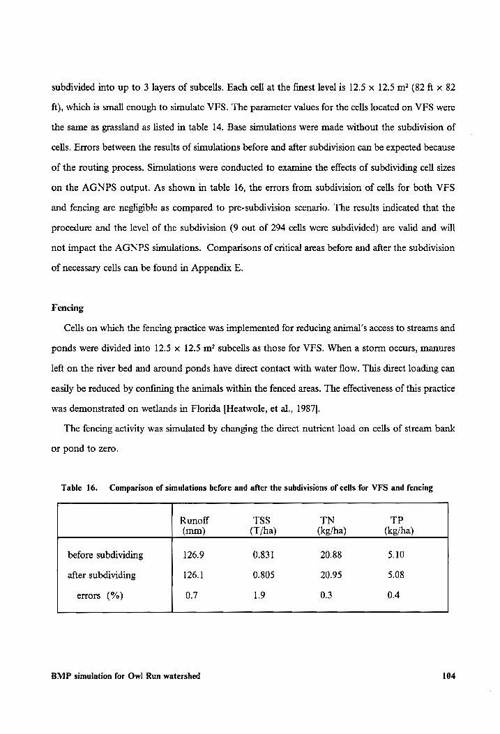
subdivided into up to 3 layers of subcells. Each cell at the finest level is 12.5 x 12.5 m? (82 ft x 82

ft), which is small enough to simulate VFS. The parameter values for the cells located on VFS were

the same as grassland as listed in table 14. Base simulations were made without the subdivision of

cells. Errors between the results of simulations before and after subdivision can be expected because

of the routing process. Simulations were conducted to examine the effects of subdividing cell sizes

on the AGNPS output. As shown in table 16, the errors from subdivision of cells for both VFS

and fencing are negligible as compared to pre-subdivision scenario. The results indicated that the

procedure and the level of the subdivision (9 out of 294 cells were subdivided) are valid and will

not impact the AGNPS simulations. Comparisons of critical areas before and after the subdivision

of necessary cells can be found in Appendix E.

Fencing

Cells on which the fencing practice was implemented for reducing animal’s access to streams and

ponds were divided into 12.5 x 12.5 m? subcells as those for VFS. When a storm occurs, manures

left on the river bed and around ponds have direct contact with water flow. This direct loading can

easily be reduced by confining the animals within the fenced areas. The effectiveness of this practice

was demonstrated on wetlands in Florida [Heatwole, et al., 1987].

The fencing activity was simulated by changing the direct nutrient load on cells of stream bank

or pond to zero.

Table 16. Comparison of simulations before and after the subdivisions of cells for VFS and fencing

Runoff TSS TN TP

(mm) (T/ha) (kg/ha) (kg/ha)

before subdividing 126.9 0.831 20.88 5.10

after subdividing 126.1 0.805 20.95 5.08

errors (%) 0.7 1.9 0.3 0.4

BMP simulation for Owl] Run watershed 104


The 1987 Chesapeake Bay Agreement stated that, by the year 2000, at least a 40 percent re-

duction in nitrogen and phosphorus entering the main stem of the Chesapeake Bay is to be achieved

due to the implementation of a basin-wide BMP strategy [U.S. EPA, 1983].

As mentioned at the beginning of this chapter, seven BMP scenarios were simulated using the

annualization procedure to evaluate their long term impacts on reducing nonpoint source pollution

losses. Results are compared to the pre-BMP scenario in terms of percent reductions in pollutant

loadings. The long term simulation results along with total cost of each scenario and cost per unit

for each scenario are given in table 18.

The conditions and corresponding parameters used for the pre-BMP simulations were described

in model validation and annualization sections (Tables 5 and 6). The pre-BMP simulation results

are provided in annualization section (Tables 11, 12, and 13), and are also listed in table 18 for

comparison purposes.

The costs to the State of Viginia for no-till, stripcropping, installation of animal waste facilities,

and other various BMP implementations were adapted from the Virginia Agricultural BMP Cost

Share Program [VDCR-DSWC, 1990]. Analyses related to cost effectiveness of BMP implemen-

tations were made based on the state of Virginia cost-share payments for various practices.

Table 17 lists Virginia state cost share rates for major BMPs. The current state funding rate for

implementing no-till practice is $37/ha/year. Cost for stripcropping systems is $74/ha/year. The

CRP was implemented under the title “Reforestation of Erodible Crop and Pastureland”, and

“Protective for Specialty Cropland” in the Virginia Agricultural BMP Cost Share Program. Eligible

lands are those on which the soil loss may exceed the tolerance limit, T. The one-time payment

for reforestation 1s $185/ha, or $18.5/ha/year, considering the 10 year land retirement for CRP. The

annual maintenance cost can be estimated under the title “Protective Cover for Specialty Cropland”

in the Virginia cost-share program, for which the state payment rate is $24.7/ha/year. Therefore the

total annual funds for CRP are $43.2/ha/year. The state cost share payment for the construction


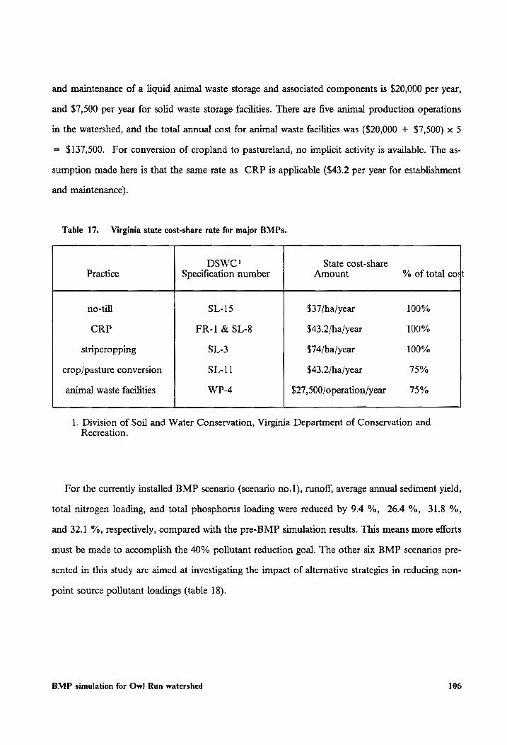
and maintenance of a liquid animal waste storage and associated components is $20,000 per year,

and $7,500 per year for solid waste storage facilities. There are five animal production operations

in the watershed, and the total annual cost for animal waste facilities was ($20,000 + $7,500) x 5

= $137,500. For conversion of cropland to pastureland, no implicit activity is available. The as-

sumption made here is that the same rate as CRP is applicable ($43.2 per year for establishment

and maintenance).

Table 17. Virginia state cost-share rate for major BMPs.

_DSWC! State cost-share | Practice Specification number Amount % of total cost

no-till SL-15 $37/ha/year 100%

CRP FR-! & SL-8 $43.2/ha/year 100%

stripcropping SL-3 $74/ha/year 100% -

crop/pasture conversion SL-11 $43.2/ha/year 75%

animal waste facilities WP-4 $27,500/operation/year 75% 1. Division of Soil and Water Conservation, Virginia Department of Conservation and

Recreation.

For the currently installed BMP scenario (scenario no.1), runoff, average annual sediment yield,

total nitrogen loading, and total phosphorus loading were reduced by 9.4 %, 264 %, 31.8 %,

and 32.1] %, respectively, compared with the pre-BMP simulation results. This means more efforts

must be made to accomplish the 40% pollutant reduction goal. The other six BMP scenarios pre-

sented in this study are aimed at investigating the impact of alternative strategies in reducing non-

point source pollutant loadings (table 18).


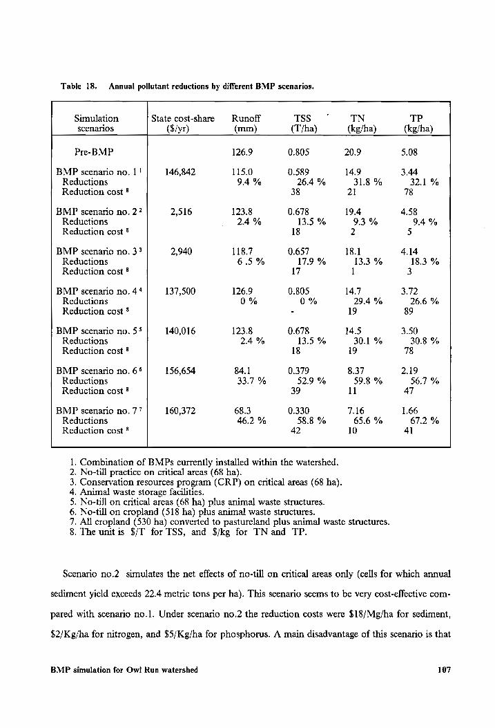
Table 18. Annual pollutant reductions by different BMP scenarios.

Simulation State cost-share Runoff TSS ™ TP scenarios ($/yr) (mm) (T/ha) (kg/ha) (kg/ha)

Pre-BMP 126.9 0.805 20.9 5.08

BMP scenario no. |! 146,842 115.0 0.589 14.9 3.44 Reductions 94% 26.4 % 31.8 % 32.1 % Reduction cost 8 38 21 78

BMP scenario no. 2? 2,516 123.8 0.678 19.4 4.58 Reductions 2.4 % 13.5 % 9.3% 94% Reduction cost 8 18 2 5

BMP scenario no. 33 2,940 118.7 0.657 18.1 4.14 Reductions 6.5% 17.9 % 13.3 % 18.3 % Reduction cost ® 17 1 3

BMP scenario no. 44 137,500 126.9 0.805 14.7 3.72 Reductions 0% 0% 29.4 % 26.6 % Reduction cost ® - 19 89

BMP scenario no. 55 140,016 123.8 0.678 14.5 3.50 Reductions 2.4 % 13.5 % 30.1 % 30.8 % Reduction cost ® 18 19 78

BMP scenario no. 6 156,654 84.1 0.379 8.37 2.19 Reductions 33.7 % 52.9 % 59.8 % 56.7 % Reduction cost ? 39 11 47

BMP scenario no. 77 160,372 68.3 0.330 7.16 1.66 Reductions 46.2 % 58.8 % 65.6 % 67.2 % Reduction cost ® 42 10 41

. Combination of BMPs currently installed within the watershed. No-till practice on critical areas (68 ha).

. Conservation resources program (CRP) on critical areas (68 ha). Animal waste storage facilities. No-till on critical areas (68 ha) plus animal waste structures.

. No-till on cropland (518 ha) plus animal waste structures.

OIANRWNE

. All cropland (530 ha) converted to pastureland plus animal waste structures.

. The unit is $/T for TSS, and $/kg for TN and TP.

Scenario no.2 simulates the net effects of no-till on critical areas only (cells for which annual

sediment yield exceeds 22.4 metric tons per ha). This scenario seems to be very cost-effective com-

pared with scenario no.1. Under scenario no.2 the reduction costs were $18/Mg/ha for sediment,

$2/Kg/ha for nitrogen, and $5/Kg/ha for phosphorus. A main disadvantage of this scenario is that


the amounts of pollutant reductions are far less than the 40% reduction goal (13.5 %, 9.3% and

9.4 % reductions for sediment yield, nitrogen and phosphorus loadings, respectively, table 18).

Scenario no.3 was designed to evaluate the impact of CRP practice on the same critical areas

as those of scenario no.2. The pollutant reductions for this scenario were 17.9 %, 13.3 %, and

18.3 % for sediment yield, nitrogen and phosphorus loadings, respectively. These reduction rates

are higher than those reported for scenario no.2 (no-till practice on critical areas), and is the most

effective scenario for reducing pollutant loadings. The costs per unit pollutant reduction were

$17/Mg/ha for sediment, $1/Kg/ha for nitrogen, and $3/Kg/ha for phosphorus.

Scenario no.4 evaluates the impact of the installation of the animal waste storage facilities on

nutrient reductions. The cost of this practice is very high -- $137,500 for the installation and

maintenance per year for the five dairy operations. The unit costs for pollutant reductions are also

much higher than those of no-till and CRP scenarios (no.2 and no.3), respectively, but the practice

does reduce a great amount of pollutants loadings, 29.4% for N and 26.6% for P respectively. The

costs of the animal waste structures were actually even higher than those figures used in this study

because of the implementation problems encountered [Mclellen, 1990].

Scenario no.5 considers the effects of the combination of no-till and animal waste structures on

reducing nonpoint source pollution. The pollutant reductions are about the same as those of the

current BMPs, 30.1 % and 30.8 % for nitrogen and phosphorus, respectively, but the total cost

is less than scenario no.1 ($140,016 vs $146,842). Obviously, the reductions made by this scenario

are still not enough to meet the 40% goal.

None of the above five scenarios met the 40% reduction requirement. Therefore, two additional

scenarios were considered to explore the possibilities for fulfilment of the goal. Scenario no.6 as-

sesses no-till practice on all of the agricultural land plus the installation of animal waste facilities,

and scenario no.7 considers a hypothetical situation where all the croplands are converted to

pastureland in addition to the installation of animal waste structures. It should be noted that these

two scenarios may not be as practical as the ones already discussed. As shown in table 18, the

sediment, nitrogen, and phosphorus loadings could be reduced by 52.6 %, 59.8 %, and 56.7 % for

scenario no.6, and 58.8 %, 65.6 %, and 67.2 % for scenario no.7, respectively. The costs per kg


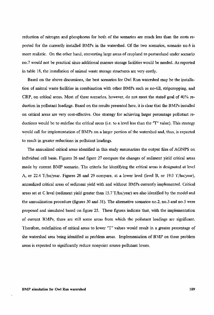
reduction of nitrogen and phosphorus for both of the scenarios are much less than the costs re-

ported for the currently installed BMPs in the watershed. Of the two scenarios, scenario no.6 is

more realistic. On the other hand, converting large areas of cropland to pastureland under scenario

no.7 would not be practical since additional manure storage facilities would be needed. As reported

in table 18, the installation of animal waste storage structures are very costly.

Based on the above discussions, the best scenarios for Owl Run watershed may be the installa-

tion of animal waste facilities in combination with other BMPs such as no-till, stripcropping, and

CRP, on critical areas. Most of these scenarios, however, do not meet the stated goal of 40% re-

duction in pollutant loadings. Based on the results presented here, it is clear that the BMPs installed

on critical areas are very cost-effective. One strategy for achieving larger percentage pollutant re-

ductions would be to redefine the critical areas (i.e. to a level less than the “IT” value). This strategy

would call for implementation of BMPs on a larger portion of the watershed and, thus, is expected

to result in greater reductions in pollutant loadings.

The annualized critical areas identified in this study summarizes the output files of AGNPS on

individual cell basis. Figures 26 and figure 27 compare the changes of sediment yield critical areas

made by current BMP scenario. The criteria for identifying the critical areas is designated at level

A, or 22.4 T/ha/year. Figures 28 and 29 compare, at a lower level (level B, or 19.0 T/ha/year),

annualized critical areas of sediment yield with and without BMPs currently implemented. Critical

areas set at C level (sediment yield greater than 15.7 T/ha/year) are also identified by the model and

the annualization procedure (figures 30 and 31). The alternative scenarios no.2, no.3 and no.5 were

proposed and simulated based on figure 25. These figures indicate that, with the implementation

of current BMPs, there are still some areas from which the pollutant loadings are significant.

Therefore, redefinition of critical areas to lower “T” values would result in a greater percentage of

the watershed area being identified as problem areas. Implementation of BMP on these problem

areas is expected to significantly reduce nonpoint source pollutant losses.


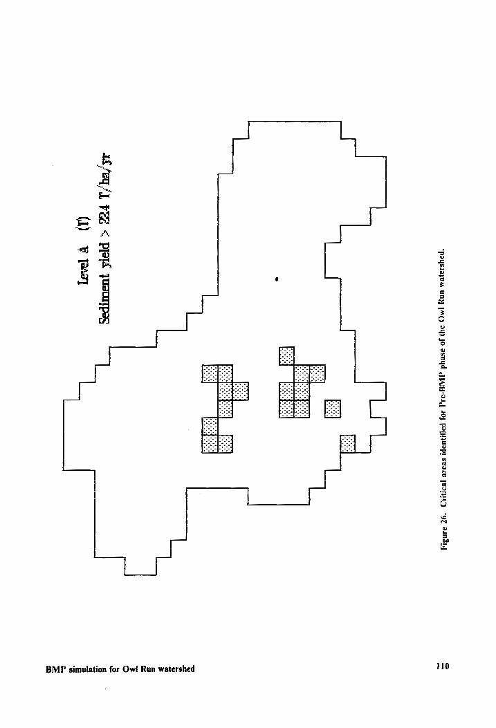
“payssazeM UNY

|AC) 34}

JO BsVyd

FAL-FAc

40J PIYNWUIP!

SCIIG PEIN

°97Z ainsi]

rer

eee

eee

oened

were

eseeg

Anecieath wer

eee?

ry vee

e Paes

eh oo ae

oane

pote e

eB ietete®

owe

toe

oe ‘

on toe

tee

fe *

eee

’ o

as beast

eoaa

teen

‘ ee

see

oe

ewes

va

. .

’ eae

ee

eone

Ge eae

¢ a

a .

.

iS Eq‘

Fee <

PPLE JOscoTpag

110

(1) ¥

Te]

BMP simulation for Ow! Run watershed

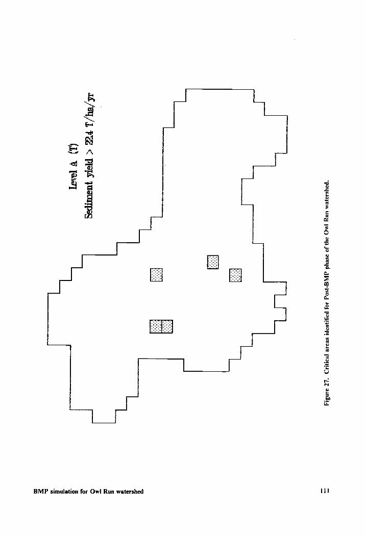
*PpayssajzUAa UNY

JMO 3y3

JO aseyd

QA/Y-ISOg 10)

pAyQuap! sease

pean

°2Z aansiy

etre

Peree

rerr

soe

eee

eres

. sneer

oeae

eee

ers

' .

i /Eq/L Fee

< PRL

yosopes

(1) ¥

[sey

111 BMP simulation for Owl Run watershed

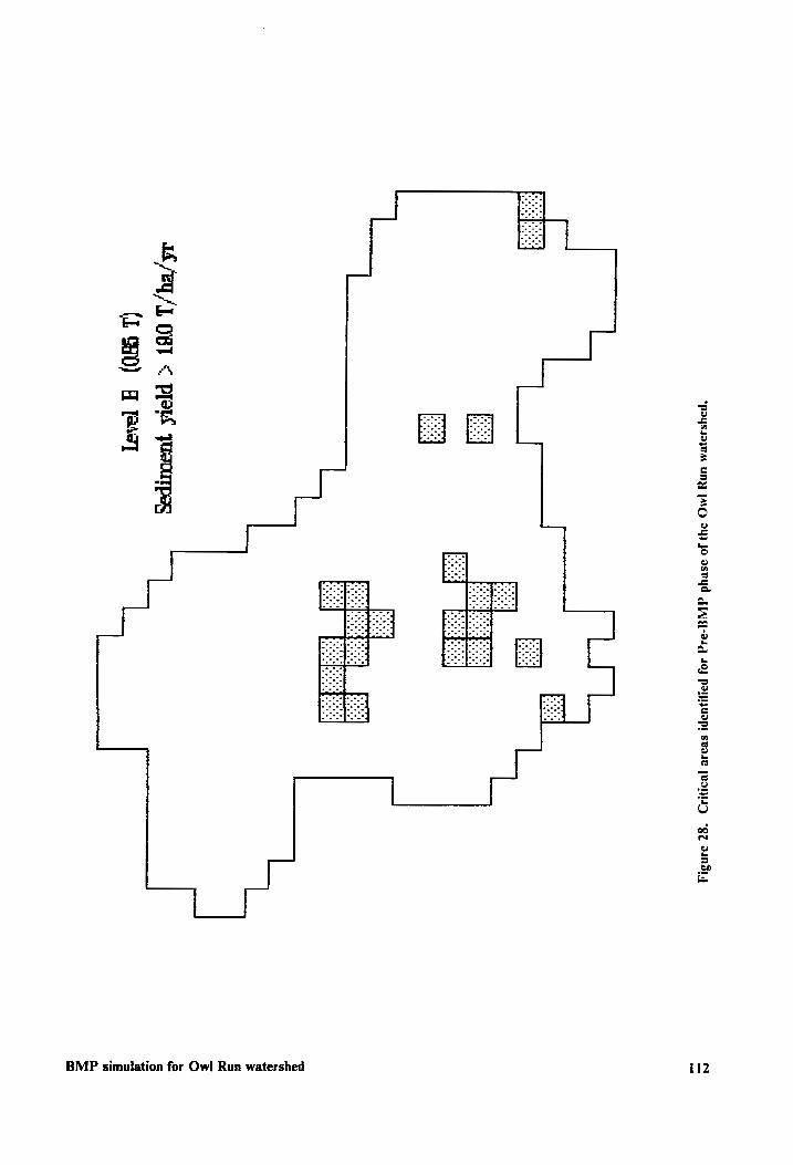
*payssajyem uny

FAC 24)

JO aseyd

IAg]-34,] 40}

payluaps svase

peony

“gz 34N31,)

fn eore

q Ppeves

ene

ee ‘

oe es

eee

wees

one

Peeos

tage

eons

veea

' teen

erates «eee

eno

see

tana

ve eon

tee

oun

rear

eee

anes

tons

tease

oe

het

‘ oe

oe a

earn

de oe

. oe

ee ee

. .

a6 feq/1 OBT

< PIPL JusoMTpeg

(L S90)

A 9]


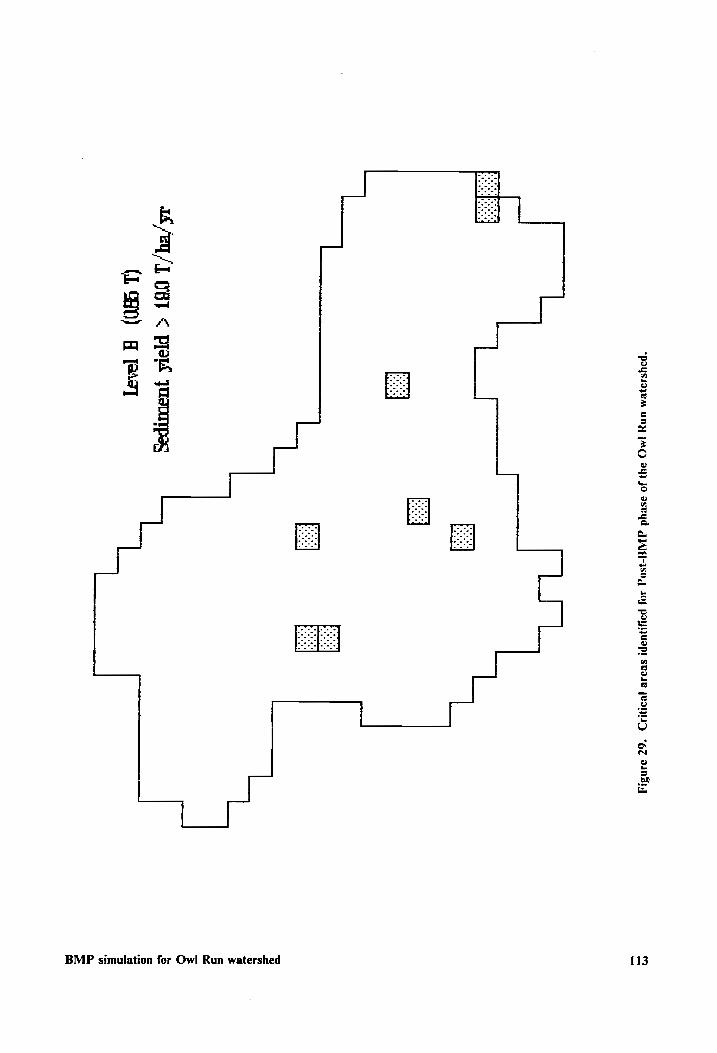
*poysuazem UNY

[MG 24)

JO aseyd

GIALY-3SOq JOJ

payHuapi sass

peony

*6Z aan

6 /2q/] OBT

< PIsKt

yuscorpag

(1 G0)

Af [asa]


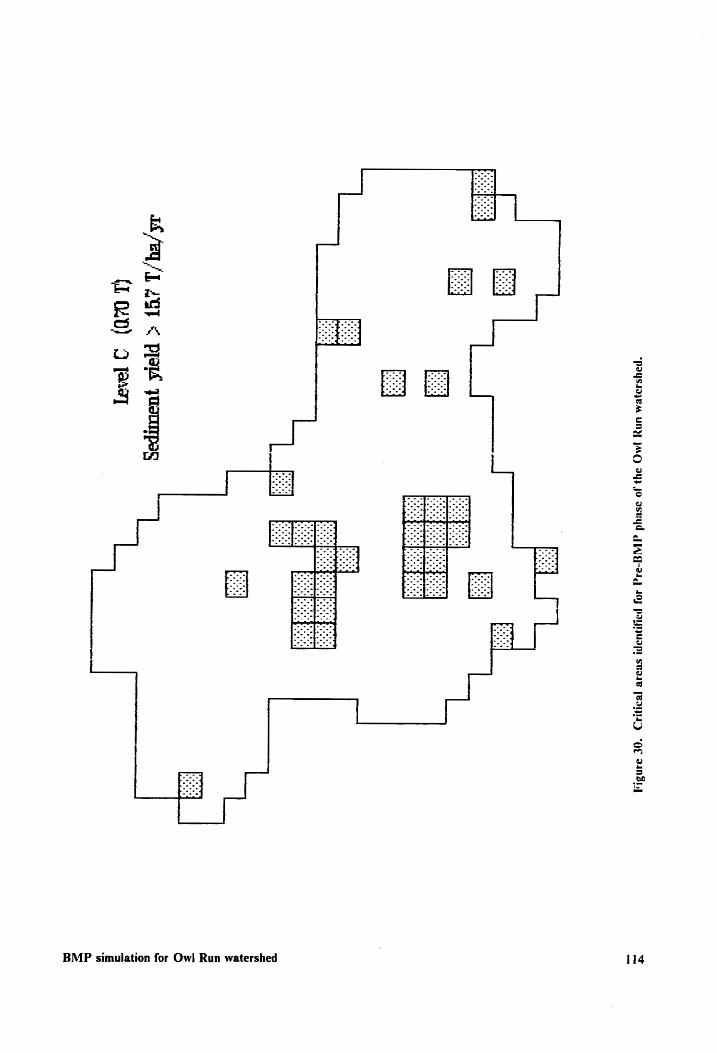
Payssayem UNY

JMG IY}

Jo aseyd

GIAG-F%f 40}

paypyuapl svase

peau

‘gg angi]

ee ne

eae w

eee

8 ee

eee

eee

eere

ene

eee.

feos

we ‘

yore

ve ee

nas

eaee

soe

If /EG/L LOT

< pret

yusonpag

(1 O40)

3 9]


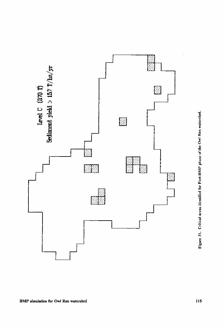
paysiajzem uny

[MO 243

JO aseyd

GFIAI-ISOg 40J

payNnuops Sease

pesnUD *|¢

andy

eeengq

.

I /EQ/L 2ST

< pists

pOSoOTpeg

(Lh 0)

3 a]

11S BMP simulation for Owl Run watershed

Summary and conclusions

The overall goal of this study was to investigate the applicability of an appropriate NPS pol-

lution model to small watersheds in Virginia Piedmont areas. Several distributed watershed models

were reviewed and a suitable model, AGNPS, which has the ability to evaluate effectiveness of

specific BMPs, was selected for this study. The model has been widely accepted because of its

simplicity, comprehensiveness, ability to consider spatial variability of watershed characteristics, and

its ability to identify critical areas study areas.

The model was validated by comparing model predictions with data collected from a small ag-

ricultural watershed in the area. The data used for validation were recorded by a meteorological,

hydrological, and water quality monitoring system installed in the Owl Run watershed.

An annualization procedure was used to convert the event based simulation results of the model

to average annual results so that the BMP effectiveness was evaluated on a long-term basis. The

long-term simulation results were also compared with recorded average annual data from the study

watershed. Nonpoint source pollution critical areas on the watershed were identified by using the

model and the annualization procedure, and some applicable BMPs were proposed, based on the

critical areas, for reducing pollutant loadings. The effectiveness of the proposed BMP scenarios were

then evaluated by the model.

Summary and conclusions 116

The annualization procedure was applied under several assumptions. Surface cover conditions

for preparation of model parameters were assumed to be uniform within each period considered for

the year; the antecedent soil moisture condition-II was used to represent the average antecedent soil

moisture conditions; and rainfall and EI values were considered to be uniformly distributed

throughout the watershed.

The following conclusions were made from this study:

Runoff, sediment yield, nitrogen and phosphorus loadings predicted by AGNPS compared rea-

sonably well with the observed data as indicated by simple linear regression analyses, comparison

of mean values, and relative errors represented by root mean square (rms) error methods.

The applicability of the annualization procedure for AGNPS to the study area was demonstrated

by comparing simulated runoff volume, sediment yield, and N and P loadings with those collected

from the watershed during a three-year period. Relative errors of 23.5%, 14.3%, and 8.9% were

calculated for sediment yield, N and P loadings for the average three year data collected from the

watershed.

The impact of BMPs currently installed in watershed, as well as those of six proposed BMP

scenarios on reducing nonpoint source pollutant loadings to the streams were simulated with

AGNPS. The expected average long-term reductions in pollutant loadings due to the implementa-

tion of current BMPs were 31.8% for N, 32.1% for P, and 26.4% for sediment.

Scenario no.2 and no.3, proposed for evaluating impact of no-till or CRP implementations on

critical areas, were found to be the most cost effective in reducing pollutant loadings. The no-till

scenario (no.2) could reduce sediment yield by 13.5%, and N and P losses by 9.2% and 9.4%, re-

spectively, with the costs of $18/T/year for sediment, $2/kg/year for N loss, and $5/kg/year for P

loss. Scenario no.3 reduces sediment by 17.9%, N by 13.3%, and P by 18.3%, with reduction costs

of $17/T/year, $1/kg/year, and $3/kg/year for sediment yield, N, and P losses, respectively. Animal

waste facility scenario (no.4) has the largest impact on reducing N and P loadings (29.4% and


26.6%, respectively), but fairly high unit reduction costs of $19.5/kg for N, and $89.0/kg for P. The

total annual cost for this scenario is $137,500.

The most effective and practical scenario seems to be somewhere between scenarios no.5 (no-till

on Critical areas plus animal waste facilities) and no.6 (no-till on all agricultural land plus animal

waste facilities). Scenario no.6 could reduce N and P loadings by 59.8% and 56.7%, respectively,

which meets the 40% reduction goal, with a total annual cost of $155,654, just slightly higher than

that of the current scenario. It should be noted, however, that the Chesapeake Bay agreement has

recommended reducing nutrients loadings to the Bay by 40 percent to protect long-term water

quality. Nutrients loadings from small watersheds located in the headwaters of the Bay, such as

Owl Run watershed, however, may need to be reduced by a larger percentage to achieve this goal.

Due to the complexity of the procedures involved, however, it is not possible to accurately estimate

the percent reduction needed at the headwaters.

It should be mentioned that input data preparation for distributed model parameters such as

those of AGNPS is very time consuming and difficulties will arise in determing accurate values for

some parameters. Based on the results obtained from this study, however, it appears that AGNPS

is a suitable model for application to Virginia Piedmont conditions.


Recommendations

The following recommendations are presented for further research on application of NPS pol-

lution models to small watersheds:

1. A mainframe version of AGNPS is necessary because of the large computation load and

memory space requirement. For annualized simulations performed in this study, the average long

term values of pollutant loadings were obtained based on a two dimensional analysis of seasonal

variation and magnitude of storms (i.e. the probability distributions of the model output were

functions of seasonal variation and magnitude of the representative events). If the frequency ana-

lyses of antecedent soil moisture conditions and/or other factors are taken into account, the com-

putation time will increase substantially.

2. In this study , two seasons, dormant and growing, were used for hydrologic and water quality

simulation. To better describe the seasonal variations of the parameters related to surface cover

conditions, more seasonal stages (periods) within the year should be considered.

Recommendations 119

3. Better relationships between rainfall amount and erosion index of storm events need to be

explored. Representative storm events can be analyzed as two dimensional joint frequency distrib-

utions of rainfall amount and erosion index for each storm event.

4. The seasonal variability of antecedent soil moisture conditions needs to be investigated. In this

study the average condition (condition-IJ) as classified by the National Engineering Handbook,

section-4 [USDA-SCS, 1972] was assumed. Frequency analysis of this parameter will help reduce

errors in using the annualization procedure.

5. Additional research is necessary on determining the fertilization levels and availability factors

for AGNPS. Relationship between the levels and the rate of animal waste or chemical fertilizer

application needs to clarified and the values need to be categorized in more detail.

6. Simulation of individual BMPs using AGNPS needs to be validated. This requires long term

monitoring data to compare with the simulation results.

7. A technique based on operations research, expert system, or other system analysis or opti-

mization theories is useful to identify feasible BMP combinations and select the best ones

8. Interfacing AGNPS input files with GIS is necessary to make more efficient analyses with

smaller cell sizes.

Recommendations 120

Bibliogrophy

Arnold, J.G., J.R. Williams. 1987. Validation of SWRRB --- Simulator for water resources in rural basins. Journal of Water Resources Planning and Management, Vol. 113, No.2.

ASAE. 1988. ASAE standards-1988. Structures, livestock, and environment. D384. pp 427.

Bagnold, R.A. 1966. An approach to the sediment transport problem from general physics. Prof. Paper 422-J. U.S. Geol. Survey, Reston, VA.

Beasley, D.B., L.F. Huggins, and E.J. Monke. 1980. ANSWERS: A model for watershed planning. Transactions of ASAE 23(4): 938-944.

Beasley, D.B., L.F. Huggins, and E.J. Monke. 1982. A monitoring/modeling strategy for 208 implementation. Transactions of the ASAE 25(3):654-660,665.

Beasley, D.B., L.F. Huggins. 1982. ANSWERS user’s manual. EPA-950/9-82-001. U.S.D.A. Region 5, Chicago, IL, 54pp.

Beasley, D.B., and W.C. Mills. 1989. A preliminary evaluation of ANSWERS in the Georgia coastal plain. Presentation at the 1989 international meeting jointly sponsored by ASAE and CSAE. Quebec, PQ, Canada.

Bennett, M.R., T.A. Dillaha, J.A. Burger, S. Mostaghimi, and V.O. Shanholtz. 1990. Water quality modeling for nonpoint source pollution control planning: Nutrient transport. MS thesis. Dept. of Ag. Engineering, Virginia Tech. Blacksburg, VA.

Beven, K. 1985. Distributed models. In hydrological Forecasting. Chapter 13. John Wiley & Sons Ltd.

Bingner, R.L., C-E. Murphree, and C.K. Mutchler. 1989. Comparison of Sediment Yield Models on Watersheds in Mississippi. Transactions of the ASAE. Vol. 32(2), pp. 529-544.

Breve, M.A., D.L. Thomas, J.M. Sheridan, D.B. Beasley, and W.C. Mills. 1989. A preliminary evaluation of ANSWERS in the Georgia Coastal Plain. Presentation at the 1989 international summer meeting of ASAE and CSAE, Quebec, PQ, Canada.

Bibliogrophy 121

Chow, V.T. 1953. Design charts for finding rainfall intensity frequency, Water and Sewage Works, vol 9, no 2, pp. 86-88, Feb., 1952.

Chow, V.T. 1955. On the determination of frequency factor in log-probability plotting, Trans. Am. Geophys. Union, vol. 36, pp. 481-486.

Chow, V.T. 1964. Handbook of Applied Hydrology -- A compendium of water resources technology. Mcgraw-Hill book company. p.8-9.

Cook, D.J., W.T. Dickinson, and R.P. Rudra. 1985. GAMES --- the Guelph model for evaluating effects of agricultural management systems on erosion and sedimentation. University of Guelph, School of Engineering Tech. Rep. 126-71, Guelph, Ontario.

Council on Environmental Quality. 1980. Environmental Quality -- 1980: The eleventh annual report of the council on environmental quality. U.S. Gov. Print. Off., Washington, DC.

Crawford, H.H., and R.K. Linsley. 1966. Digital simulation in hydrology: Stanford Watershed Model-4. TR No.39. Stanford University, Stanford, Calif. 210pp.

Crowder, B.M. 1987. Issues in water quality modeling of agricultural management practices: An economic perspective. p.313-327. Proceedings of the symposium on monitoring, modeling and mediating water quality, May 1987. American Water Resources Association, Minneapolis, MN.

Davis, H.H. Jr., and A.S. Donigian, Jr.. 1979. Simulating nutrient movement and transformations with the ARM model. Transactions of the ASAE 22(1): 151-154.

De Roo, A.P.J., L. Hazelhoff, and P.A. Barrough. 1989. Soil erosion modeling using ANSWERS and Geographic Information System. Earth Surface Processes and Landforms, Vol. 14, 517-532(1989).

DeCoursey, D.G. 1985. Mathematical models for nonpoint water pollution control. Journal of Soil and Water Conservation Sept-Oct, 1985. pp. 408.

Dempster, T.H., and J.H. Stierna. 1979. Procedures for economic evaluation of Best Management Practices. In Best Management Practices for agriculture and silviculture. R.C. Loehr et al., eds. Ann Arbor Sci. Publ. Inc., Ann Arbor, MI.

Dickinson, W.T., R.P. Rudra, and E.L. Von Euw. 1989. Sensitivity of a nonpoint source model to rainfall data. Presentation at the 1989 international summer meeting sponsored by ASAE and CSAE. Quebec, PQ, Canada.

Dillaha, T.A. and D.B. Beasley. 1983. Distributed parameter modeling of sediment movement and particle size distributions. Transactions of the ASAE 26(6): 1766-1777.

Donigian, A.S. 1982. Water quality modeling in relation to watershed hydrology. In V.P. Sinph [ed.]} Modeling components of Hydrologic Cycle. Water Resources Publications, Littleton, Colo. pp. 343-382.

Donigian, A.S. Jr., J.C. Imhoff and B.R. Bicknell. 1983. Predicting water quality resulting from agricultural nonpoint source pollution via simulation -- HSPF. Agricultural Management and Water Quality. Edited by F.W. Schaller and G.W. Bailey. Iowa St. Univ. Press. Ames, Iowa.

Donigian, A.S. Jr., and H.H. Davis, Jr.. Users Manual for Agricultural Runoff Monagement (ARM) Model. EPA-600/3-78-080, Environmental Research Laboratory, U.S. EPA. Athens, GA. 293p.

Bibliogrophy 122

Duttweiler, D.W., and H.P. Nicholson. 1983. Environmental problems and issues of agricultural nonpoint source pollution. In Agricultural Management and Water quality. Iowa St. Univ. Press. Ames, Iowa. p3-16.

Feezor, D.R., M.C. Hirschi, and B.J. Lesikar. 1989. Effect of cell size on AGNPS prediction. Presentation at the 1989 ASAE international winter meeting. New Orleans, Louisiana.

Foster, G.R., D.K. McCool, K.G. Renard, and W.C. Moldenhauer. 1981. Conversion of the Universal Soil Loss Equation to SI Metric Units. Journal of Soil and Water Conservation, Nov.-Dec. 1981. pp.355-359.

Foster, H.A. 1924. Theoretical frequency curves and their application to engineering problems. Transactions of ASCE, vol. 87, pp.142-173.

Foster, G.R., L.J. Lane, J.D. Nowlin, J.M. Laflen, and R.A. Young. 1981. Estimating erosion and sediment yield on field-sized areas. Transactions of ASAE 24(5): 1,53-1,262.”

Frere, M.H., J.D. Ross, and L.J. Lane. 1980. The nutrient submodel CREAMS, A field scale model for Chemicals, Runoff and Erosion from Agricultural Management Systems. Conserv. Res. Rep. No.26, ARS, USDA, Washington, D.C. pp65-85.

Gilley, J.E. L.J. Lane, J.M. Laflen, A.D. Nicks, and W.J. Rawls. 1988. USDA-Water Erosion Prediction Project: New generation erosion prediction technology. In proceedings of the 1988 International Symposium. Hyatt Regency. Chicago in Illinois Center, Chicago, Illinois.

Gumbel, E.J. 1941. The return period of flood flows. Ann. Math. Statist., vol 7, no. 2, pp. 163-190.

Haan, C.T. 1977. Statistical methods in hydrology. The Iowa State University Press. Ames, lowa 50010.

Haan, C.T., H.P. Johnson, and D.L. Brakensiek. 1982. Hydrologic modeling of small watersheds. An ASAE monograph. No.5 in a series published by ASAE, 2950 Niles Rd. St. Joseph, Michigan.

Heatwole, C.D., A.B. Bottcher, and L.B. Baldwin. 1986. Basin scale model for evaluating Best Management Practice implementation programs. Transaction of the ASAE. Vol. 29(2), pp. 439-444,

Heatwole, C.D., A.B. Bottcher, and K.L. Campbell. 1987. Basin scale water quality model for Coastal Plain Flatwoods. Transaction of the ASAE. Vol. 30(4), pp.1023-1030.

Heatwole, C.D., K.L. Campbell, A.B. Bottcher. 1987. Modified CREAMS Hydrology Model for Coastal Plain Flatwoods. Transactions of the ASAE. Vol. 30, No.4 pp.1014-1022. 1987.

Hern, S.C., 1986. Vadose zone modeling of organic pollutants. Lewis Pulishers.

Hedden, K.F., 1986. Example field testing of soil fate and transport model, PRZM, Dougherty Plain, Georgia. In Vadose Zone modeling of Organic Polluatants. $.C. Hern and S.M. Melancon, Eds. Lewis Publishers, Inc. Chelsea, MI. pp. 81-101.

Holland, D.D. 1971. Sediment yields from smll drainge areas in Kansas. Bull. No.16. Kansas Water Resources Board. Topeka, KS.

Holtan, H.N. 1961. A concept for infiltration estimates in watershed engineering. Agricultural Research Service, U.S.D.A. ARS-41-51. 25p.

Bibliogrophy 123

Huggins, L.F., and EJ. Monke. 1966. The mathematical simulation of the hydrology of small watersheds. Water Resources Research Center, Purdue Univ. Technical Report 1. 130p.

Johanson, R.C., J.C. Imhoff, H.H. Davis, J.L. Kittle, and A. 8. Donigian. 1981. User’s manual for hydrologic simulation program-(HSPF). Release 7.0. U.S. Environmental Protection Agency, Athens, CA.

Knisel, W.G. 1980. CREAMS: A field-scale model for chemicals, runoff, and erosion from agricultural management systems. Conservation Research Report No. 26. Washington, D.C. USDA-SEA.

Knisel, W.G., and V. Svellosanov (ed). 1982. European and United States case studies on application of the CREAMS model. Collaborative Paper CP-82-S11, International Institute for Applied System Analysis, Laxeuburg, Austria.

Koelliker, J.K. and C.E. Humbert. 1989. Application of AGNPS model for water quality planning. Presentation at the 1989 international summer meeting sponsored by ASAE and CSAE. Quebec, PQ, Canada.

Lane, L.J. 1982. Development of a procedure to estimate runoff and sediment transport in ephemeral streams. In Recent Developments in the Explanation and Prediction of Erosion and Sediment Yield. Publ. No.137. Int. Assoc. Hydro. Sci., Willingford, England. pp275-282.

Leonard, R.A., W.G.Knisel, and D.A. Still. 1987. GLEAMS: Groundwater loading effects of agricultural management system. Transactions of the ASAE. 30(5): 1403-1418.

Laflen, J.M., H.P. Johnson, and R.O. Hartwig. 1978. Erosion modeling on impoundment terraces. Transactions of ASAE 21(6):1,131-135.

Linsley, R.K. jr., Max A. Kohler, and J.L.H. Paulhus. 1988. Hydrology for engineers. SI metric edition. McGraw-Hill book company.

Madramootoo, C.A., L. Laperriere and S.F. Barrington. 1988. Modeling runoff and sediment yields from Quebec watersheds. In: Modeling agricultural, forest and rangeland hydrology. Proceedings of the 1988 international symposium; Dec. 12-13; Chicago, IL. St. Joseph, MI. ASAE; 1988: 264-270.

Masse, L., and S.O. Prasher. 1989. Field verification of GLEAMS in Eastern Canada. Presenta- tion at the 1989 Winter Meeting of ASAE. St. Joseph, MI.

Meyer, L.D.; and W.H. Wischmeier. 1969. Mathematical simulation of the processes of soil erosion b water. Transactions of the ASAE. 12(6): 754-758.

Mostaghimi, S., P.W. McClellan, U.S. Tim, J.C. Carr, R.K. Byler, T.A. Killaha, V.O. Shanholtz, and J.R. Pratt. 1989. Watershed/water quality monitoring for evaluating animal waste BMP effectiveness -- Owl Run watershed. Pre-BMP final report. Report No. O-P1-8906.

Mostaghimi, S., U.S. Tim, P.W. McClellan, J.C. Carr, R.K. Byler, T.A. Dillaha, and V.O. Shanholtz. 1988. Watershed/water quality monitoring for evaluating BMP effectiveness -- Nomini Creek watershed. Pre-BMP Evaluation report. Report No. N-P1-8811.

Needham, S. and P.E. Baxter Vieux. 1989. A GIS for AGNPS parameter input and mapping output. Presentation at the 1989 international winter meeting sponsored by ASAE. New Orleans, Louisiana.

Bibliogrophy 124

Novotny, V. 1986. A review of hydrologic and water quality models used for simulation of agricultural pollution. p. 9-35. In: Giorgini, A and F Zingules [ed.] Agrucultural nonpoint source pollution: Model selection and application. Elsevier Science Publishing Co., Inc. New York. 409 p.

Overton, D.E. 1964. Mathematical refinement of an infiltration equation for watershed engineering. ARS-41-99, Agricultural Research Service, USDA. Ip.

Ozga-Zielinska, Maria, 1976. Structure and operation functions of mathematical models of hydrologic systems. J. Hydrologic Science (Poland), 3(1,2):1-20.

Park, S.W., J.K. Mitchell and J.N. Scarborough. 1982. Soil erosion simulation on small watersheds: A modified ANSWERS model. Transactions of the ASAE 25(5):1581-1588.

Pearson, Karl, 1930. Tables for statisticians and biometricians, Part 1, The Biometric Laboratory, University College, London; printed by Cambridge University Press, London, 3d ed.

Putman, J., J.R. Williams, and D. Sawyer. 1988. Using the erosion-productivity impact calculator (EPIC) model to estimate the impact of soil erosion for the 1985 RCA appraisal. J. of Soil and Water Conservation. Vol. 43, No.4, July-August pp. 321-326.

Robert, P.C., J.L. Anderson, C.A. Bunn, and R.A. Young. 1985. Agricultural nonpoint source pollution program for personal microcomputers. Dept. of soil science. Minnesota Extension Service, Univ. of Minnesota.

Ross, B.B., M.L. Wolfe, et al. 1982. Model for simulating runoff and erosion in ungaged watersheds. Bulletin 130. Virginia Water Resources Research Center, VPI&SU, Blacksburg, VA.

Ross, B.B., V.O. Shanholtz, et al. 1978. A model for evaluating the effect of land uses on flood flows. Bulletin 85. Virginia Water Resources Research Center, VPI&SU, Blacksburg, VA. ”

Ross, G.A. 1970. The Stanford Watershed Model: The correlation of parameter values selected by a computerized procedure with measurable physical characteristics of the watershed. Water Resources Institute Research Report No. 35. Univ. of Kentucky, Lexington, KY.

Rudra, R.P., W.T. Dickinson, D.J. Clark, and G.J. Wall. 1986. GAMES --- A screening model of soil erosion and fluvial sedimentation. Canadian Water Resources Journal 11(4): 58-71.

Soil Conservation Service. 1956. Soil survey of Fauquier County, Virginia. Series 1944, No.7. In cooperation with the Virginia Agricultural Experiment Station.

Soil Conservation Service. 1979. Westmoreland County Soil Survey. Nat. Coop. Soil Survey. U.S. Dept. of Agriculture.

Shaffer, N.J., S.C. Gupta, D.R. Linder, J.A. Molina, and W.E. Larson. 1983. Nitrogen-tillage- residue-management model (NTRM). In Analysis of Ecological Systems: State of the Art in Ecological Models. Elsevier Pub., New York, N.Y. pp. 525-544.

Shanholtz, V.0O., M.D. Smolen, D.F. Amos, and J.B. Burger. 1981. Predicting soil loss from surface mined areas. State Mining And Mineral Resources Research Inst. VPI&SU, Blacksburg, Virginia.

Shanholtz, V.O., P.A. Hellmund, R.K. Byler, S. Mostaghimi, and T.A. Dillaha. 1987. VirGIS, agricultural pollution potential data base - phase 1. Final Report. VirGIS Laborary, Depart- ment of Agricultural Engineering, Virginia Tech, Blacksburg, VA.

Bibliogrophy 125

Shirmohammadi, A., T.J. Gish, D.E. Lehman, W.L. Magette. 1989. GLEAMS and the vadose zone modeling of pesticide transport. Presentation at the 1989 international summer meeting. Quebec, PW, Canada. June, 1989.

Smith, M.C., K.L. Campbell, A.B. Bottcher, and D.L. Thomas. 1989. Field testing and comparison of the PRZM and GLEAMS models. ASAE paper. 89-2082. ASAE, St. Joseph, MI 49085.

Smith, R.E., and Hebbert, R.H. 1979. A Monte Carlo analysis of the hydrologic effects of spatial variability of infiltration. Water Resources Research 15, 419-429.

Smith, R.E., and J.R. Williams. 1980. Simulation of surface water hydrology. In CREAMS, a Field Scale Model for Chemicals, Runoff, and Erosion from Agricultural Management Sys- tems. Conservation Research Report. 26. Agr. Res. Serv. USDA, Washinton, DC. p15.

Storm, D.E., 1987. Identification and modeling of critical watersheds for nonpoint source pollution control: Sediment and phosphorus. MS thesis, Dept. of Age, VWPI&SU, Blacksburg, VA.

Storm, D.E., T.A. Dillaha, S. Mostaghimi, and V.O. Shanholtz. 1988. Modeling phosphorus transport in surface runoff. Transactions of ASAE. 31(1):117-127.

Tchobanoglous, G., and I.D. Schroeder. 1985. Water quality management. Addson-Wesley Pub- lishing Company, Reading, MA.

Thamann, R.V. 1982. Verification of water quality models. J. of Environment Engineering Di- vision, ASCE 108:923-939.

Thomas, D.L., and D.B. Beasley. 1986. A physically-based forest hydrology model 1: Develop- ment and sensitivity of components. Trans. of the ASAE 29(4):962-9721.

USDA-SCS. 1984. User’s Guide for the CREAMS Computer Model. Washington computer center version. Technical Release 72.

USDA-SCS, and Virginia Agricultural Experiment Station. 1956. Soil survey -- Fauquier County, Virginia. Series 1944, No. 7.

USDA-SCS. 1972. Hydrology. In National Engineering Handbook. Washington, D.C. pp. 10.5-10.6.

USEPA. 1983. Chesapeake Bay: A framework for action. Chesapeake Bay Program. USS. Envi- ronmental Protection Agency, Annapolis, MD. 186p.

Virginia Department of Conservation and Historic Resources, Division of Soil and Water Con- servation. 1986. Owl Run livestock BMP demonstration watershed. Richmond, VA.

VDCR - DSWC (Virginia Department of Conservation and Receation, Division of Soil and Water Conservation). 1990. The Virginia Agricultural BMP Cost-Share Program Manual 1991.

Wight, J.R., editor. 1983. SPUR --- Simulator of production and utilization of rangelands. A rangeland model for management and research. Misc. Publ. No.1431. USDA, Washington, D.C. 120pp. ”

Williams, J.R. 1985. The physical components of the EPIC Model. In S.A. El-Swaify et al. (ed) Soil Erosion and Conservation. Soil Conservation Society of America, Ankeny, IA. p.272-284.

Bibliogrophy 126

Williams, J.R., and K.G. Renard. 1985. Assessments of soil erosion and crop productivity with process models (EPIC). p.67-103. In Soil Erosion and Crop Productivity. American Society of Agronomy. Crop Science Society of America. Soil Science Society of America. Madison, WI.

Wischmeier, W.H., and Smith, D.D. 1978. Predicting rainfall erosion losses. Agr. Handbook. 537 USDA, Washington, DC.

Wischmeier, W.H., and J.V. Mannering. 1969. Relation of soil properties to its erodibility. Soil Science Society of America Proceedings. V.33. pp131.

Wischmeier, W.H., C.B. Johnson, and B.V. Cross. 1971. <A soil erodibility nomograph for farmland and construction sites. Journal of Soil and Water Conservation. V.26. no.5 pp 189.

Young, G.K.K. and C.L. Alward. 1983. Calibration and testing of nutrient and pesticide transport models. In Agricultural Management and Water Quality. Ed. by F.W. Schaller and G.W. Bailey. lowa State Univ. Press, Ames, Iowa.

Young, R.A., C.A. Onstad, D.D. Bosch, and W.P. Anderson. 1987. AGNPS, Agricultural nonpoint source pollution model. A watershed analysis tool. USDA, ARS, Conservation Research Report No.35. National Technology Information Service, Springfield, VA.

Young, R.A., C.A. Onstad, et al. 1985. Agricultural nonpoint source pollution models (AGNPS) I and II model documentation. Minnesota Pollution Control Agency, St. Paul, and Agr. Res. Serv., Washington, D.C. 53pp.

Young, R.A., C.A. Onstad, et al. Oct. 1989. AGNPS user’s guide, version 3.5.

Young, R.A., C.A. Onstad, D.D. Bosch, and W.P. Anderson. 1989. AGNPS: A nonpoint source pollution model for evaluating agricultural watersheds. Journal of soil and water conservation. March-April, 1989. p. 168-173.

Young, R.A., M.A. Otterby and A. Ross. 1982. A technique for evaluating feedlot pollution potential. Journal of Soil and Water Conservation. 37(1):21-23.

Bibliogrophy | 127

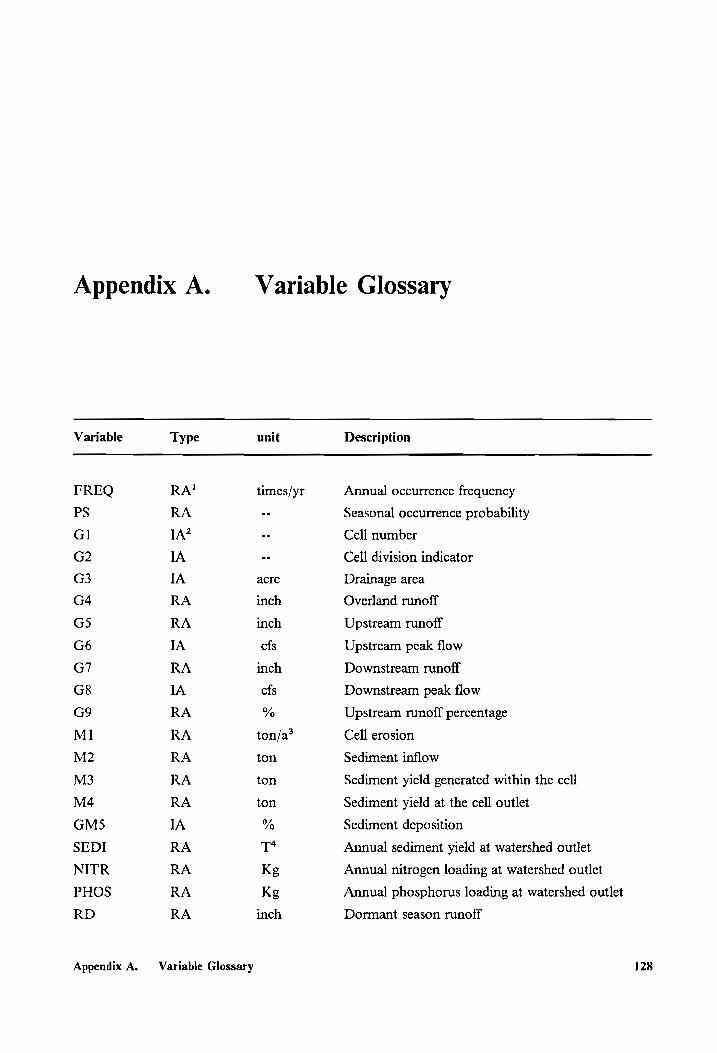
Appendix A. —— Variable Glossary

Variable Type unit Description

FREQ RA! times/yr Annual occurrence frequency

PS RA -- Seasonal occurrence probability

Gl [A? -- Cell number

G2 IA -- Cell division indicator

G3 IA acre Drainage area

G4 RA inch Overland runoff

GS RA inch Upstream runoff

G6 IA cfs Upstream peak flow

G7 RA inch Downstream runoff

G8 IA cfs Downstream peak flow

G9 RA % Upstream runoff percentage

M1 RA ton/a? Cell erosion

M2 RA ton Sediment inflow

M3 RA ton Sediment yield generated within the cell

M4 RA ton Sediment yield at the cell outlet

GMS5 IA % Sediment deposition

SEDI RA T4 Annual sediment yield at watershed outlet

NITR RA Kg Annual nitrogen loading at watershed outlet

PHOS RA Kg Annual phosphorus loading at watershed outlet

RD RA inch Dormant season runoff

Appendix A. Variable Glossary 128

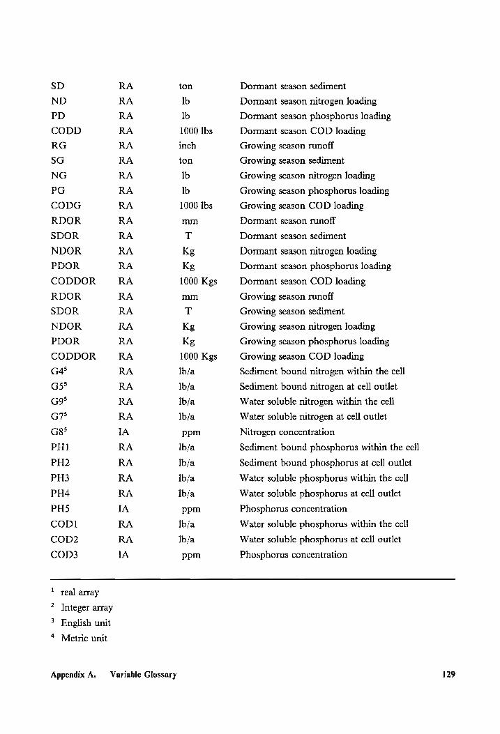
SD RA ton Dormant season sediment

ND RA Ib Dormant season nitrogen loading

PD RA lb Dormant season phosphorus loading

CODD RA 1000 Ibs Dormant season COD loading

RG RA inch Growing season runoff

SG RA ton Growing season sediment

NG RA Ib Growing season nitrogen loading

PG RA lb Growing season phosphorus loading

CODG RA 1000 Ibs Growing season COD loading

RDOR RA mm Dormant season runoff

SDOR RA T Dormant season sediment

NDOR RA Kg Dormant season nitrogen loading

PDOR RA Kg Dormant season phosphorus loading

CODDOR RA 1000 Kgs Dormant season COD loading

RDOR RA mm Growing season runoff

SDOR RA T Growing season sediment

NDOR RA Kg Growing season nitrogen loading

PDOR RA Kg Growing season phosphorus loading

CODDOR RA 1000 Kgs Growing season COD loading

G45 RA Ib/a Sediment bound nitrogen within the cell

G5> RA lb/a Sediment bound nitrogen at cell outlet

G9° RA Ib/a Water soluble nitrogen within the cell

G7? RA Ib/a Water soluble nitrogen at cell outlet

G8> IA ppm Nitrogen concentration

PH] RA Ib/a Sediment bound phosphorus within the cell

PH2 RA Ib/a Sediment bound phosphorus at cell outlet

PH3 RA Ib/a Water soluble phosphorus within the cell

PH4 RA Ib/a Water soluble phosphorus at cell outlet

PHS IA ppm Phosphorus concentration

COD1 RA Ib/a Water soluble phosphorus within the cell

COD2 RA Ib/a Water soluble phosphorus at cell outlet

COD3 IA ppm Phosphorus concentration

1 real array

Appendix A.

Integer array

3 English unit

Metric unit

Variable Glossary 129

> Reused variable in the loop for dormant season calculation.

Appendix A. ‘Variable Glossary 130

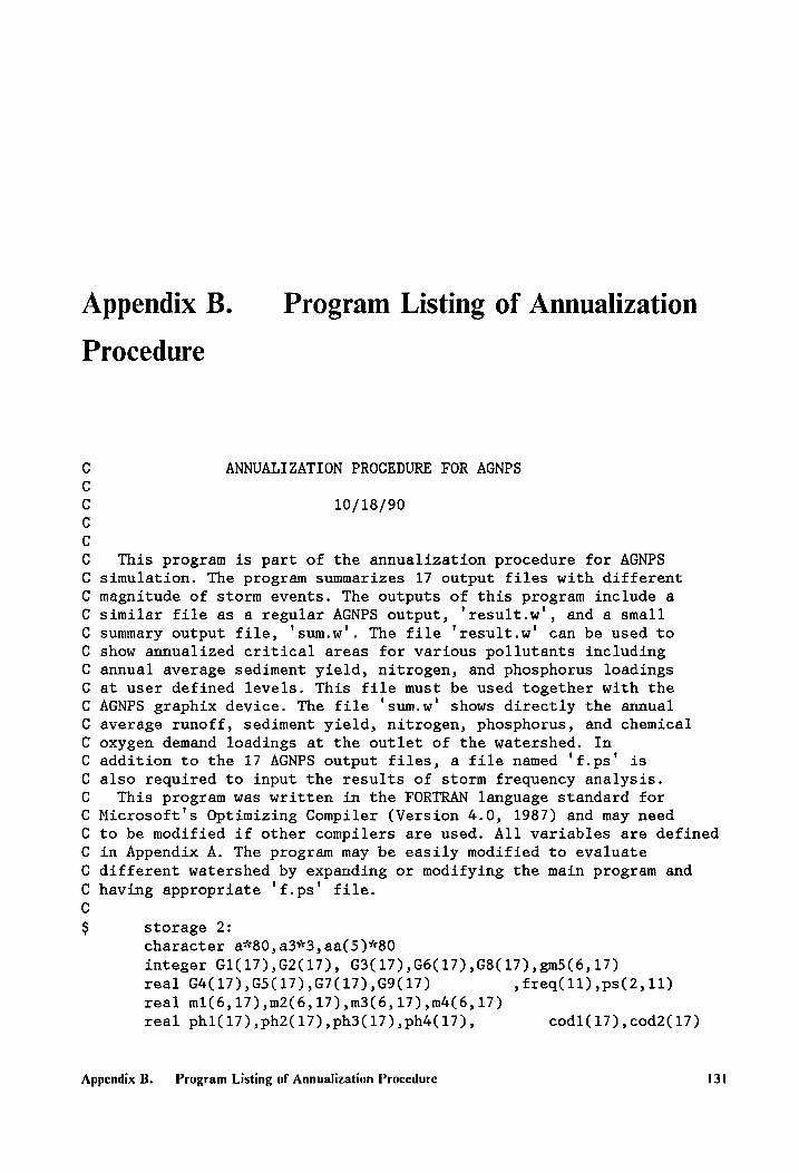
Appendix B. —_ Program Listing of Annualization

Procedure

PMPOAMIAAAAAIAIANRMAXMANANARMRAIANMQAaARAaNAaAN ANNUALIZATION PROCEDURE FOR AGNPS

10/18/90

This program is part of the annualization procedure for AGNPS simulation. The program summarizes 17 output files with different magnitude of storm events. The outputs of this program include a similar file as a regular AGNPS output, 'result.w', and a small summary output file, 'sum.w'. The file 'result.w' can be used to show annualized critical areas for various pollutants including annual average sediment yield, nitrogen, and phosphorus loadings at user defined levels. This file must be used together with the AGNPS graphix device. The file 'sum.w' shows directly the annual average runoff, sediment yield, nitrogen, phosphorus, and chemical

oxygen demand loadings at the outlet of the watershed. In addition to the 17 AGNPS output files, a file named 'f.ps' is also required to input the results of storm frequency analysis.

This program was written in the FORTRAN language standard for Microsoft's Optimizing Compiler (Version 4.0, 1987) and may need to be modified if other compilers are used. All variables are defined in Appendix A. The program may be easily modified to evaluate different watershed by expanding or modifying the main program and

having appropriate 'f.ps' file.

storage 2:

character a*80,a3*3,aa(5)*80

integer G1(17),G2(17), G3(17),G6(17),G8(17),9m5(6,17) real G4(17),G5(17),G7(17),G9(17) , freq(11),ps(2, 11) real m1(6,17),m2(6,17),m3(6,17),m4(6,17)

real ph1(17),ph2(17),ph3(17),ph4(17), cod1(17),cod2(17)

Appendix B. Program Listing of Annualization Procedure 131

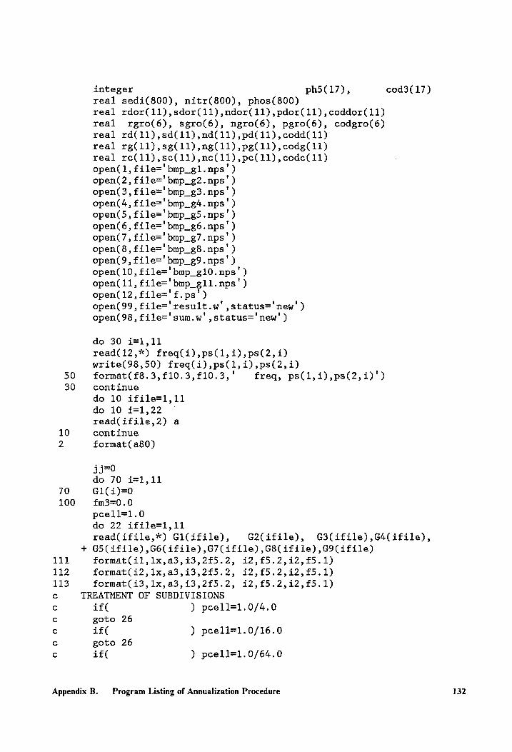
1 1 1 c

oOo aan

50 30

70 100

11 12 13

integer ph5(17), cod3(17)

real sedi(800), nitr(800), phos(800)

real rdor(11),sdor(11),ndor(11),pdor(11),coddor(11)

real rgro(6), sgro(6), ngro(6), pgro(6), codgro(6)

real rd(11),sd(11),nd(11),pd(11),codd(11)

real rg(11),sg(11),ng(11),pg(11),codg(11) real rc(11),sc(11),nc(11),pc(11),codc(11) open(1, file='bmp_gl.nps') open(2, file='bmp_g2.nps') open(3, file='bmp_g3.nps') open(4, file='bmp_g4.nps') open(5, file='bmp_g5.nps') open(6, file='bmp_g6.nps') open(7, file='bmp_g7.nps') open(8, file='bmp_g8.nps') open(9, file='bmp_g9.nps') open(10, file='bmp_g10.nps') open(11, file='bmp_gll.nps') open(12,file='f.ps') open(99, file='result.w',status='new’ ) open(98,file='sum.w',status='new')

do 30 i=1,11

read(12,*) freq(i),ps(1,i),ps(2,i) write(98,50) freq(i),ps(1,i),ps(2,i) format(£8.3,£10.3,£10.3,' freq, ps(1,i),ps(2,i)')

continue

do 10 ifile=1,11

do 10 i=1,22 —

read(ifile,2) a

continue

format(a80)

jj=0 do 70 i=1,11 G1(i)=0 fm3=0.0 pcell=1.0 do 22 ifile=1,11 read(ifile,*) Gli(ifile), G2(ifile), G3(ifile),G4(ifile), G5(ifile) ,G6(ifile) ,G7(ifile) ,G8(ifile) ,G9(ifile) format(il,1x,a3,i3,2f5.2, i2,£5.2,i2,£5.1) format(i2,1x,a3,i3,2f5.2, i2,f5.2,i2,£5.1) format(i3,1x,a3,i3,2f5.2, i2,f5.2,i2,£5.1)

TREATMENT OF SUBDIVISIONS if( ) peell=1.0/4.0 goto 26 if( ) peell=1.0/16.0 goto 26 if( )} pcell=1.0/64.0


c

O00 0

26 continue

if(Gl(ifile).gt.9) goto 180

if(Gl(ifile).gt.99) goto 181

write(98,111) GlCifile), G2(ifile), G3(ifile),G4(ifile),

+ G5(ifile) ,G6(ifile),G7(ifile) ,G8(ifile) ,G9(ifile) write(*,113) Gi(ifile), G2(ifile), G3(Cifile),G4(ifile),

+ G5(ifile),G6(ifile),G7(ifile) ,G8(ifile) ,G9(ifile) goto 86 write(98,112) Gli({ifile), G2(ifile), G3(ifile),G4(ifile),

+ G5(ifile) ,G6(ifile),G7(ifile),G8(ifile) ,G9(ifile) goto 86

write(98,113) Gl(ifile), G2(ifile), G3(ifile),G4(ifile), + G5(ifile),G6(ifile) ,G7(ifile) ,G8(ifile) ,G9(ifile)

continue

do 20 ir=1,6 read(ifile,*) mi(ir,ifile) ,m2(ir,ifile),m3(ir,ifile),

+ m4(ir,ifile),gm5(ir,ifile)

continue

fm3=fm3+m3(6, ifile)*freq(ifile)*ps(1,ifile)*pcell

if(GliCifile).ne.251) goto 22

rd(ifile)=g7(ifile)*freq(ifile)*ps(1,ifile)*pcell

sd(ifile)=m4(6,ifile)*freq(ifile)*ps(1,ifile)*pcell

rdor(ifile)=g7(ifile)*pcel1*25.4

sdor(ifile)=m4(6,ifile)*pcel1*0.9072 continue

j3=35+1 sedi(jj)=fm3

write(*,7) jj

format(i5)

if(G1(11).1t.294) goto 100

jj=0

TREATMENT OF NUTRIENTS

71 200

do 71 ifile=i,11

read(ifile,2) a

read(ifile,2) a Gic(i)=0 fni=0.0

£ph=0.0 pcell=1.0 do 282 ifile=1,11 read(ifile,*) Gi(ifile), G2(ifile), G3(ifile),

+ G4(ifile) ,G5(ifile) ,G9(ifile) ,G7(ifile) ,G8(ifile)

read(ifile,*) phl(ifile), ph2(ifile), ph3(ifile),ph4(ifile), + ph5(ifile),codl(ifile),cod2(ifile),cod3(ifile)

TREATMENT OF SUBDIVISIONS if( ) peell=1.0/4.0 goto 226 if( ) peell=1.0/16.0


226

282

289

284

310

72 300

QAaAaang

goto 226 if( ) peell=1.0/64.0

continue

fni=fnit+(G5(ifile)+G7(ifile))*freq(ifile)*ps(1,ifile)*pcell

fph=fpht+(ph2(ifile)+ph4(ifile))*freq(ifile)*ps(1,ifile)*pcell

if(Gl(ifile).ne.251) goto 282

nd(ifile)=(G5(ifile)+G7(ifile))*freq(ifile)*ps(1,ifile)*pcell

pd(ifile)=(ph2(ifile)+ph4(ifile))*freq(ifile)*ps(1,ifile)*pcell

codd(ifile)=cod2(ifile)*freq(ifile)*ps(1,ifile)*pcell

ndor(ifile)=(G5(ifile)+G7(ifile))*pcell*0.4536*2911.0

pdor(ifile)=(ph2(ifile)+ph4(ifile) )*pcel1*0.4536*2911.0

coddor(ifile)=cod2(ifile)*pcel1*0. 4536/1000. 0*2911.0

continue

§j=jjt1 nitr(jj)=fni

phos(jj)=fph write(*,7) jj

if(G1(11).1t.294) goto 200

continue

jj=0 do 284 i=1,11 close(i) open(1,file='bmp_di.nps') open(2,file='bmp_d2.nps') open(3,file='bmp_d3.nps') open(4, file='bmp_d4.nps') open(5, file='bmp_d5.nps') open(6, file='bmp_d6.nps' )

do 310 ifile=1,6

do 310 i=1,22

read(ifile,2) a

if(ifile.gt.1) goto 310 write(99,2) a

continue

do 72 i=1,6

G1(i)=0

fm3=0.0 pcell=1.0 do 322 ifile=1,6 read(ifile,*) Gl(ifile), G2(ifile), G3(ifile),G4(ifile),

+ G5(ifile) ,G6(ifile) ,G7(ifile) ,G8(ifile) ,G9(ifile)

TREATMENT OF SUBDIVISIONS if ( ) peell=1.0/4.0

goto 26 if( ) pceell=1.0/16.0


Cc goto 26 c if( ) peell=1.0/64.0

326 continue

do 320 irow=1,5

read(ifile,2) aa(irow)

320 continue

irow=6

read(ifile,*} miCirow,ifile) ,m2(irow,ifile) ,m3(irow,ifile),

+ m4(irow,ifile),gm5(irow, ifile)

fm3=fm3+m3(6,ifile)*freq(ifile)*ps(2,ifile)*pcell

if(giCifile).ne.251) goto 322

rg(ifile)=g7(ifile)*freq(ifile)*ps(2,ifile)*pcell sg(ifile)=m4(6,ifile)*freq(ifile)*ps(2,ifile)*pcell

rgro(ifile)=g7(ifile)*pcel1*25.4

sgro(ifile)=m4(6,ifile)*pcel1*0.9072

322 continue

jj=jjt+1 £m3=(fm3+sedi( jj))*0.9072/4.0 if(fm3.1t.1.00) £fm3=1.04

if(g3(1).gt.99) g3(1)=99 if(g3(1).1t.10) g3(1)=10 if(g6(1).gt.9) g6(1)=9

if(g8(1).gt.9) g8(1)=9

if((g4(1).gt.9.99).or.(g4(1).1t.1.00)) g4(1)=1.04 if((g5(1).gt.9.99).or.(g5(1).1t.1.00)) g5(1)=1.04 if((g7(1).gt.9.99).or.(g7(1).1t.1.00)) g7(1)=1.04 if((g9(1).gt.99.9).or.(g9(1).1t.10.0)) 2g9(1)=44.4 if((G1(1).gt.9).and.(G1(1).1t.100)) goto 360 if(G1(1).gt.99) goto 361

call zh(G2(1),a3)

write(99,111) G1(1),a3,G3(1),G4(1),G5(1),G6(1), + G7(1),G8(1),G9(1)

goto 366 call zh(G2(1),a3)

360 write(99,112) G1(1),a3,G3(1),G4(1),G5(1),G6(1), + G7(1),G8(1),G9(1)

goto 366 call zh(G2(1), a3)

361 write(99,113) G1(1),a3,G3(1),G4(1),G5(1),G6(1), + G7(1),G8(1),G9(1)

366 continue

do 390 ir=1,5

write(99,2) aa(ir)

390 continue

ir=6

if((m1(6,1).gt.9.99).or.(m1(6,1).1t.1.00)) m1(6,1)=1.04


114 115 116 117

316

370

314 379

93 94

if((m2(6,1).gt.9.99).or.(m2(6,1).1t.1.00)) m2(6,1)=1.04 if((m3(6,1).gt.9.99).or. (m3(6,1).1t.1.00)) m3(6,1)=1.04

if((gm5(6,1).gt.99).or.(gm5(6,1).1t.10)) gm5(6,1)=44 format (f4.2,2£5.2,£5.2 ,i3)

format(f4.2,2f£5.2,f6.2 ,i3)

format(f£4.2,2f£5.2,£7.2 ,i3)

format(f£4.2,2£5.2,£8.2 ,i3) if(fm3.1t.99.99) goto 370

if(fm3.1t.999.99) goto 316

write(99,117) ml(ir,1),m2Cir,1), m3(Cir,1),fm3, gm5(ir,1)

goto 379

write(99,116) ml(ir,1),m2(ir,1), m3(ir,1),fm3, gm5(ir,1)

goto 379

if(fm3.1t.10.00) goto 314

write(99,115) ml(Cir,1),m2(ir,1), m3(Cir,1),fm3, gm5(ir,1) goto 379 write(99,114) miCir,1),m2(Cir,1), m3(ir,1),fm3, gm5(ir,1) continue

write(*,7) jj

if(G1(6).1t.294) goto 300

write(99,93)

write(99,94) format ( Vveded! )

format ('NUTRIENT' )

c TREATMENT OF NUTRIENTS

73

400

onanan

426

Append

do 73 i=1,6 read(i,2) a

read(i,2) a

G1Ci)=0

jj=0 fni=0.0

fph=0.0 pcell=1.0 do 422 ifile=1,6

read(ifile,*) Gl(ifile), G2(ifile), G3(ifile),

+ G4(ifile),G5(ifile) ,G9(ifile) ,G7(ifile),G8(ifile) read(ifile,*) phl(ifile), ph2(ifile), ph3(ifile),ph4(ifile),

+ ph5(ifile),codl(ifile),cod2(ifile),cod3(ifile)

TREATMENT OF SUBDIVISIONS if( ) peell=1.0/4.0

goto 226 if( ) pcell=1.0/16.0 goto 226

if( ) peell=1.0/64.0

continue

fni=fnit+(G5(ifile)+G7(ifile))*freq(ifile)*ps(2,ifile)*pcell

fph=fpht+(ph2(ifile)+ph4(ifile) ) + *freq(ifile)*ps(2,ifile)*pcell

ix B. Program Listing of Annualization Procedure 136

if(gl(ifile).ne.251) goto 422

ng(ifile)=(G5(ifile)+G7(ifile))*freq(ifile)*ps(2,ifile)*pcell

pg(ifile)=(ph2(ifile)+ph4(ifile))*freq(ifile)*ps(2,ifile)*pcell

codg(ifile)=cod2(ifile)*freq(ifile)*ps(2,ifile)*pcell

ngro(ifile)=(G5(ifile)+G7(ifile) )*pcel1*0.4536*2911.0

pgro(ifile)=(ph2(ifile)+ph4(ifile) )*pce11*0.4536*2911.0 codgro(ifile)=cod2(ifile)*pcel1*0.4536/1000.0*2911.0

422 continue

jj=jj+1 fni=(fnitnitr(jj))*1.12085 fph=(fphtphos( jj))*1.12085

if(g3(1).gt.99) 23(1)=99 if(g3(1).1t.10) 23(1)=10 if((g4(1).gt.9.99).or.(g4(1).1t.1.00)) g4(1)=1.04 if((g5(1).gt.9.99).or.(€g5(1).1t.1.00)) g5(1)=1.04

if((g9(1).gt.9.99).or.(g9(1).1t.1.00)) 2g9(1)=1.04

if(g8(1).gt.9) g8(1)=9 if((ph1(1).gt.9.99).or.(ph1(1).1t.1.00)) phi(1)=1.04 if((ph2(1).gt.9.99).or.(ph2(1).1t.1.00)) ph2(1)=1.04 if((ph3(1).gt.9.99).or. (ph3(1).1t.1.00)) ph3(1)=1.04 if((€cod1(1).gt.9.99).or.(cod1(1).1t.1.00)) cod1(1)=4.44 if((cod2(1).gt.9.99).or. (cod2(1).1t.1.00)) cod2(1)=4.44

if((cod3(1).gt.99).or.(cod3(1).1t.10)) cod3(1)=44

if(ph5(1).gt.9) ph5(1)=9

211 format(il,1x,a3,i3,3f5.2,f5.2,12) 221 format(il,1x,a3,i3,3£5.2,f6.2,i2) 231 format(il,1x,a3,i3,3f5.2,£7.2,i2) 241 format(il,1x,a3,i3,3f£5.2,£8.2,i2) 251 format(il,1x,a3,i3,3£5.2,f9.2,i2) 212 format(i2,1x,a3,i3,3f5.2,f5.2,i2) 222 format(i2,1x,a3,i13,3f5.2,f6.2,i2) 232 format(i2,1x,a3,i3,3f5.2,f7.2,i2) 242 format(i2,1x,a3,i3,3f£5.2,f8.2,i2) 252 format(i2,1x,a3,i3,3f5.2,£9.2,i2) 213 format(i3,1x,a3,i3,3f£5.2,f5.2,i2) 223 format(i3,1x,a3,i3,3f5.2,f6.2,i2) 233 format(i3,1x,a3,i3,3f£5.2,f7.2,i2) 243 format(i3,1x,a3,i3,3f5.2,£8.2,1i2) 253 format(i3,1x,a3,i3,3f£5.2,£9.2,i2) 214 format(£4.2,2f£5.2,£5.2,i2,2f5.2,i3) 224 format (f£4.2,2f£5.2,f6.2,i2,2f5.2,i3)

234 format(f£4.2,2f5.2,£7.2,12,2f5.2,1i3) 244 format(f4.2,2f5.2,£8.2,12,2f5.2,i3)

fni=fni*100.0 fph=fph*100.0

if(fni.1t.1.00) fni=1.04 if(fph.1t.1.00) fph=1.04 assign 214 to kp


591

592

560

593

561

594

Appendix B.

if(fph

assign

if(fph assign

if(fph

assign

.1t.10.00) goto 591 224 to kp .1t.100.00) goto 591 234 to kp -1t.1000.00) goto 591 244 to kp

continue

if((G1(1).gt.9).and.(G1(1).1t.100)) goto 560

if(G1(1).gt.99) goto 561

call zh(G2(1),a3)

assign

if(fni. assign

if(fni.

assign

if(fni.

assign

if(fni. assign

211 to kn 1t.10.00) goto 592 221 to kn 1t.100.00) goto 592 231 to kn 1t.1000.00) goto 592 241 to kn 1t.10000.00) goto 592 251 to kn

continue

write(99,kn) G1(1),a3,G3(1),

write(99,kp) phl(1),ph2(1),ph3(1),

G4(1),G5(1),69(1), fni, G8(1)

fph, ph5(1),cod1(1),cod2(1),cod3(1)

goto 526

assign

if(fni.

assign

if(fni. assign

if(fni. assign

if(fni. assign

212 to kn 1t.10.00) goto 593 222 to kn

1t.100.00) goto 593 232 to kn 1t.1000.00) goto 593 242 to kn 1t.10000.00) goto 593

252 to kn continue

call zh(G2(1),a3)

write(99,kn) G1(1),a3,G3(1),

write(99,kp) ph1l(1),ph2(1),ph3(1),

G4(1),G5(1),G9(1), fni, G81)

fph, ph5(1),cod1(1),cod2(1),cod3(1)

goto 526 assign

if(fni.

assign

if(fni. assign

if(fni.

assign

if(fni. assign

213 to kn

1t.10.00) goto 594 223 to kn

1t.100.00) goto 594 233 to kn

1t.1000.00) goto 594 243 to kn 1t.10000.00) goto 594 253 to kn

continue

call zh(G2(1),a3)

Program Listing of Annualization Procedure 138

write(99,kn) G1(1),a3,G3(1), G4(1),G5(1),G69(1), fni, G8(1) write(99,kp) phi(1),ph2(1),ph3(1), fph,

+ ph5(1),cod1(1),cod2(1),cod3(1)

526 continue

write(*,7) jj if(G1(6).1t.294) goto 400

write(99,93)

do 610 i=1,6

rd(i)=(rd(i)t+rg(i))*25.4 sd(i)=(sd(i)+sg(i))*0.9072

nd(i)=(nd(i)+ng(i))*2911*0.4536

pd(i)=(pd(i)+pg(i))*2911*0.4536 610 codd(i)=(codd(i)+codg(i))*2911*0.4536/1000.0

do 611 i=7,11 rd(i)=rd(i)*25.4 sd(i)=sd(i)*0.9072

nd(i)=nd(i)*2911*0. 4536 pd(i)=pd(i)*2911*0.4536

611 codd(i)=codd(i)*2911*0.4536/1000.0 run=0.0

sed=0.0

tn=0.0

tp=0.0 tcod=0.0

do 612 i=1,11

run=runtrd(i)

sed=sedt+sd(i) tn=tntnd(i)

tp=tptpd(i) 612 tcod=tcod+codd(i)

do 613 i=1,11

re(i)=rd(i)/run*100.0

sc(i)=sd(i)/sed*100.0

nce(i)=nd(i)/tn*100.0

pe(i)=pd(i)/tp*100.0

613 codc(i)=codd(i)/tcod*100.0

write(98,621) rd,run, re 621 format(/11f£6.1,£8.1/11f6.1)

write(98,622) sd,sed, sc

622 format(/11f6.1,£8.1/11f6.1)

write(98,623) nd,tn, ne

623 format(/11f6.0,£9.0/11f6.1)

write(98,624) pd,tp, pe 624 format(/11£6.0,£9.0/11£6.1)

write(98,625) codd,tcod, codc 625 format(/11£6.1,£9.1/11£6.1)

write(98,631) rdor,rgro


631 format(///8X, 'DIRECT SIMULATION'//2f6.3,2f6.2,7£6.2/ + £6.3,5f6.2)

write(98,632) sdor,sgro

632 format(/11£6.1/11f6.1)

write(98,633) ndor,ngro

633 format(/3f5.0,4f6.0,4f£7.0/11£6.0) write(98,634) pdor, pgro

634 format(/7£6.0,4£7.0/11£6.0) write(98,635) coddor,codgro

635 format(/11f6.1/11f6.1)

end

subroutine zh(n, a3)

character a3*3,b(3),b3*3 equivalence (b(1),b3) il=n/100+48

i2=mod(n, 100) /10+48 i3=mod(mod(n, 10),10)+48

b(1)=CHAR(I1) B(2)=char(i2)

b(3)=char(i3)

a3=b3

end


Vita

Yang Wang was born on May 30, 1955 in Beijing, China. He received a B.Eng. degree in

Agricultural Water Resource Engineering from North China Institute of Water Conservancy and

Hydropower, Handan, Hebei Province, China in February, 1981. He was an assistant engineer in

the Northwest Research Institute of Water Resources Engineering, Yangling, Shaanxi Province,

China for two years and then entered the graduate school of the same college for two and half years

graduate study. He received the M.Eng. degree in July, 1986. He worked as a research engineer in

the same research institute in northwest China for another two years before entering Virginia Tech

to pursue an MS in Agricultural Engineering in August, 1988. He plans to begin studies in January,

1991 towards a PhD at another university in the United States.

Vita 141

Documents

Nhe Le ptr — ke VF el