nhess-10-2021-2010 Didenkulova Anderson

Nat. Hazards Earth Syst. Sci., 10, 2021–2029, 2010www.nat-hazards-earth-syst-sci.net/10/2021/2010/doi:10.5194/nhess-10-2021-2010© Author(s) 2010. CC Attribution 3.0 License.

Natural Hazardsand Earth

System Sciences

Freak waves of different types in the coastal zone of the Baltic Sea

I. Didenkulova1,2 and C. Anderson3

1Laboratory of Wave Engineering, Institute of Cybernetics, Tallinn, Estonia2Department of Nonlinear Geophysical Processes, Institute of Applied Physics, Nizhny Novgorod, Russia3Department of Probability and Statistics, University of Sheffield, Sheffield, UK

Received: 9 June 2010 – Revised: 5 August 2010 – Accepted: 11 August 2010 – Published: 30 September 2010

Abstract. We present a statistical analysis of freak waves1

measured during the 203 h of observation on sea surface el-evation at a location in the coastal zone of the Baltic Sea(2.7 m depth) during June–July 2008. The dataset contains97 freak waves occurring in both calm and stormy weatherconditions. All of the freak waves are solitary waves, 63% ofthem having positive shape, 17.5% negative shape and 19.5%sign-variable shape. It is suggested that the freak waves canbe divided into two groups. Those of the first group, whichincludes 92% of the freak waves, have an amplification factor(ratio of freak wave height to significant wave height) whichdoes not vary from significant wave height and has valueslargely within the range of 2.0 to 2.4; while for the secondgroup, which contain the most extreme freak waves, ampli-fication factors depend strongly on significant wave heightand can reach 3.1. Analysis based on the Generalised Paretodistribution is used to describe the waves of the first groupand lends weight to the identification of the two groups. Itis suggested that the probable mechanism of the generationof freak waves in the second group is dispersive focussing.The time-frequency spectra of the freak waves are studiedand dispersive tracks, which can be interpreted as dispersivefocussing, are demonstrated.

1 Introduction

There has been much recent interest in the problem of freak(rogue) wave occurrence. It has been realised that in manysituations, extreme single waves can cause significant dam-age to marine structures and even lead to failure, and a num-

Correspondence to:I. Didenkulova([email protected])

1taken to be waves whose height is 2 or more times greater thanthe significant wave height

ber of ship accidents have been caused by freak waves (Tof-foli et al., 2005; Didenkulova et al., 2006). As a result, muchattention has been paid to freak wave occurrence in the deeppart of the ocean with regards to ship accidents and dam-age to ocean platforms. The North and Norwegian Sea, fromwhich many accidents have been reported, has become a fo-cus of intense study of freak waves (Magnusson et al., 1999;Bitner-Gregersen and Magnusson, 2004; Guedes Soares etal., 2004; Stansell, 2004; Walker et al., 2004; Petrova et al.,2006; Krogstad et al., 2008; Olagnon, 2008), but extremewave data have also been analysed for the Mediterranean(Prevosto et al., 2000), Japan Sea (Mori and Yasuda, 2002),Gulf of Mexico (Al-Humoud et al., 2002) and Kuwaiti ter-ritorial waters (Neelamani et al., 2007). Different theoret-ical models of freak wave generation have been developed(Olagnon and Athanassoulis, 2001; MaxWave, 2003; Kharifand Pelinovsky, 2003; Kharif et al., 2009).

Freak wave events are also observed near shore, wherethey can lead to damage to coastal structures and loss oflife. For example, Chien et al. (2002), report on 140 freakwave events in the coastal zone of Taiwan for the past50 years (1949–1999) and Didenkulova et al. (2006), reporton coastal freak wave events seen by casual eyewitnessesin 2005. The increased incidence of such accidents sug-gests more widespread coastal freak wave occurrence thanhas hitherto been recognized. Usually freak events onshoreresult in sudden short-term flooding of the coast, or a strongimpact upon steep banks or coastal structures. Some descrip-tions of such events are given in Dean and Dalrymple (2002)and Kharif et al. (2009). General properties of wind-wavebackground in shallow water are studied, for example, inGlukovskij (1966), Bitner (1980), Massel (1989, 1996), andYoung and Babanin (2009).

The properties of coastal freak waves and the mechanismsof their formation differ from those developed for deep wa-ters, and need to be studied. This paper presents an analysisof data on freak waves occurring in the coastal zone of the

Published by Copernicus Publications on behalf of the European Geosciences Union.

http://creativecommons.org/licenses/by/3.0/

2022 I. Didenkulova et al.: Freak waves of different types in the coastal Baltic Sea

Figure 1. The Baltic Sea, Tallinn Bay, the study site on the SW coast of Aegna (right lower

panel).

16

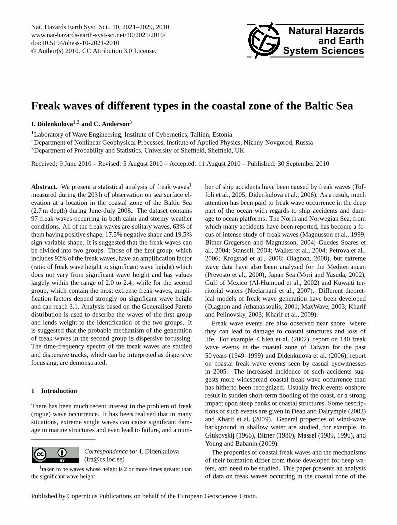
Fig. 1. The Baltic Sea, Tallinn Bay, the study site on the SW coastof Aegna (right lower panel).

Baltic Sea. The characteristic features of the Baltic Sea andthe observation site are described in Sect. 2, together with de-tails of the experiment and measurement methods. The gen-eral properties of the observed freak waves (wave heights,wave asymmetry and wave shapes) are described in Sect. 3.In Sect. 4, two putative groups of freak waves are identifiedin terms of the amplification factors and their variations withsignificant wave height. The first group, Group I (amplifica-tion factors vary over a limited range (from 2.0 to 2.4) and donot depend on significant wave height), the largest of the two,containing 92% of the freak waves observed, is discussed inSect. 5. The second group, Group II, contains more extremewaves with amplification factors reaching as high as 3.1 inthe dataset, and showing strong dependence on significantwave height. This group is studied in Sect. 6. It is suggestedthat the probable mechanism of the generation of waves inthis group is dispersive focussing. The paper concludes witha summary of findings in Sect. 7.

2 Study site and wave measurements

Tallinn Bay is a semi-enclosed body of water, approximately10×20 km in size, with the City of Tallinn located at itssouthern end. The bay belongs to a family of semi-shelteredbays that penetrate deep into the southern coast of the Gulfof Finland (Fig. 1), an elongated sub-basin of the Baltic Sea.The overall hydrodynamic activity is fairly limited in thisalmost-tideless area. There are, however, extensive waterlevel variations driven primarily by weather systems, witha maximum recorded range of 2.42 m. As very high (morethan 1 m a.m.s.l.) water level events are rare, the wind-waveimpact is concentrated into a relatively narrow range in thecoastal zone.

The complex shape of the Baltic Sea, combined with theanisotropy of predominant winds, results in a particular local

wave climate in Tallinn Bay. Most storms blow from the SWbut occasionally very strong NNW storms occur. Long andhigh waves created in the Baltic Proper during SW stormsusually do not enter the Gulf of Finland owing to geometricalblocking (Caliskan and Valle-Levinson, 2008). Bottom re-fraction at the mouth of the Gulf of Finland may cause wavesto enter the gulf under certain circumstances (Soomere et al.,2008). However, on entering they keep propagating along theaxis of the Gulf of Finland and affect only very limited sec-tions of the coast of Tallinn Bay, the northern part of which isadditionally sheltered by the islands of Aegna and Naissaar(Fig. 1). The same is also true for waves excited in the Gulfof Finland by easterly winds. The roughest seas in TallinnBay occur during NNW storms that have fetch length in theorder of 100 km and, thus, only produce waves with rela-tively short periods. These features severely limit the periodsof the wave components. The peak periods of wind wavesare usually well below 3 s, reaching 4–6 s in strong stormsand only in exceptional cases do they exceed 7–8 s.

As a result of these factors, the local wave climate is rel-atively mild in Tallinn Bay compared with the adjacent seaareas. The significant wave height exceeds 0.5–0.75 m in thebay with a probability of 10% and 1.0–1.5 m with a prob-ability of 1% (Soomere, 2005). On the other hand, veryhigh (albeit relatively short) waves occasionally occur dur-ing strong NW-NNW winds, to which Tallinn Bay is fullyopen. The significant wave height typically exceeds 2 m at acertain time each year and may reach 4 m in extreme NNWstorms in the central part of the bay. As a consequence, mostof the coast of Tallinn Bay has preserved features, indica-tive of periods of intense erosion (Lutt and Tammik, 1992;Kask et al., 2003) and, as such, it can be considered to be amedium- or high-energy coastal environment.

The wind-wave measurements were performed at the SWcoast of Aegna in the Tallinn Bay (Fig. 1). The island,about 1.5×2 km in size, is located at the northern entranceof Tallinn Bay. It is separated from the Viimsi Peninsulaby a shallow-water (typical depth 1–1.5 m) channel with twosmall islands. Effectively, no wave energy enters Tallinn Bayfrom the east.

The experimental site is fully open to the south. The max-imum fetch length in this direction, however, is only some10 km. Although the majority of storms blow from the SW,they produce no large waves. Moreover, these waves ap-proach the shore perpendicularly. Significant wave energyenters Tallinn Bay from the north but the study site is shel-tered from these waves by the island and shallow water about300 m to the west. The most significant waves at the studysite and along the adjacent shore to the west, come from thewest, entering Tallinn Bay between the mainland and the is-land of Naissaar. Waves from the NW are effectively blockedby Talneem Point (the W-SW end of Aegna, Fig. 1) and evenif they reach the SW coast owing to refraction, they impactthe coast in a similar way to waves approaching from thewest.

Nat. Hazards Earth Syst. Sci., 10, 2021–2029, 2010 www.nat-hazards-earth-syst-sci.net/10/2021/2010/

I. Didenkulova et al.: Freak waves of different types in the coastal Baltic Sea 2023

Towards Talneem, from the study site, a very shallow areaextends seaward, some 300 m from the coast, where waterdepths increase over a short distance. In the vicinity of thestudy site, water depths increase over a short distance to ap-proximately 2 m, beyond which there is a more or less linearslope from the position of the tripod on which the measur-ing equipment was mounted down to depths of 6–8 m and agently sloping terrace, 0.5–1 km wide to about 15 m waterdepth.

High resolution time series of water surface eleva-tions were collected using an ultrasonic echosounderLOG aLevel® from General Acoustics. The measurementrange of the sensor was 0.5–10 m to the water surface withan accuracy of± 1 mm. The surface water elevation datawere collected almost continuously over 30 days (21 June–20July 2008) at a recording frequency of 5 Hz. The device wasmounted at a distance of about 100 m offshore from an effec-tively non-reflecting shore of the island of Aegna at a depthof ∼2.7 m. A part of the experiment was performed in al-most calm conditions (significant wave height below 10 cm).The typical significant wave height was 30 cm and the heightreached 60 cm during short time intervals.

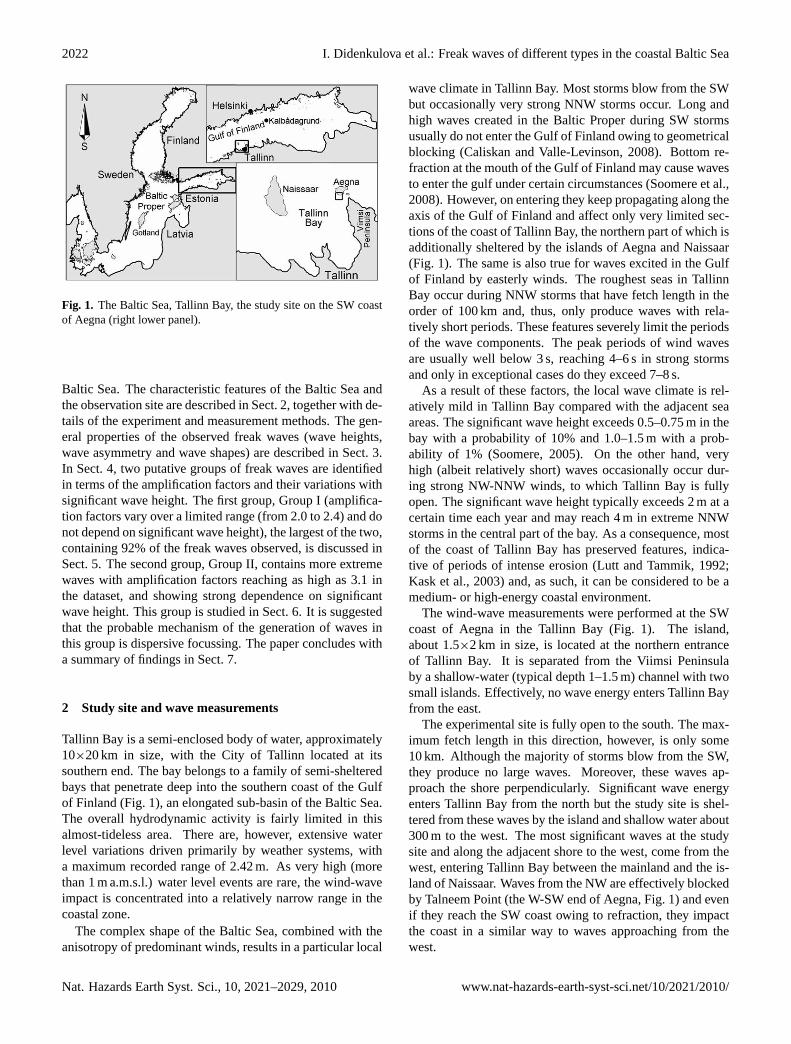
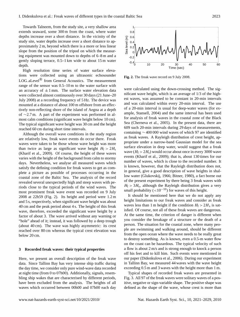
Although the overall wave conditions in the study regionare relatively low, freak wave events do occur there. Freakwaves were taken to be those whose wave height was morethan twice as large as significant wave heightHf > 2Hs(Kharif et al., 2009). Of course, the height of these wavesvaries with the height of the background from calm to stormydays. Nevertheless, we analyse all measured waves whichsatisfy the defining condition for freak waves to get as com-plete a picture as possible of processes occurring in thecoastal zone of the Baltic Sea. The analysis of the recordrevealed several unexpectedly high and steep waves with pe-riods close to the typical periods of the wind waves. Themost prominent freak wave event was recorded on 9 July2008 at 22h59 (Fig. 2). Its height and period were 1.2 mand 5 s, respectively, when significant wave height was about40 cm and the peak period about 4 s. The height of this freakwave, therefore, exceeded the significant wave height by afactor of about 3. The wave arrived without any warning or“hole” ahead of it; instead, it was followed by a deep trough(about 40 cm). The wave was highly asymmetric: its crestreached over 80 cm whereas the typical crest elevation wasbelow 20 cm.

3 Recorded freak waves: their typical properties

Here, we present an overall description of the freak wavedata. Since Tallinn Bay has very intense ship traffic duringthe day time, we consider only pure wind-wave data recordedat night time (from 0 to 07h00). Additionally, signals, resem-bling ship wakes that are characterised by different periods,have been excluded from the analysis. The heights of allwaves which occurred between 00h00 and 07h00 each day

0 10 20 30 40 50 60-0.4

-0.2

0

0.2

0.4

0.6

0.8

1

Time (sec)

Sea

leve

l (m

)

Figure 2. The freak wave record on 9 July 2008.

17

Fig. 2. The freak wave record on 9 July 2008.

were calculated using the down-crossing method. The sig-nificant wave height, which is an average of 1/3 of the high-est waves, was assumed to be constant in 20-min intervalsand was calculated within every 20-min interval. The useof a 20-min interval is usual for deep-water waves (for ex-ample, Stansell, 2004) and the same interval has been usedfor analysis of freak waves in the coastal zone of the BlackSea (Cherneva et al., 2005). In the present data, there are609 such 20-min intervals during 29 days of measurements,containing∼ 400 000 wind waves of which 97 are identifiedas freak waves. A Rayleigh distribution of crest height, ap-propriate under a narrow-band Gaussian model for the seasurface elevation in deep water, would suggest that a freakwave (Hf > 2Hs) would occur about once in every 3000 waveevents (Kharif et al., 2009); that is, about 130 times for ournumber of waves, which is close to the recorded number. Itis known, however, that the Rayleigh distribution does not,in general, give a good description of wave heights in shal-low water (Glukovskij, 1966; Bitner, 1980), a fact borne outof the present experiment by there being 3 freak waves withHf > 3Hs, although the Rayleigh distribution gives a verysmall probability (<10−10) for waves of this height.

It should be mentioned here that we do not apply anyheight limitations to our freak waves and consider as freakwaves less than 1 m height if the conditionHf > 2H s is sat-isfied. Of course, not all of these freak waves are dangerous.At the same time, the criterion of danger is different whenyou consider the breakage of a structure or the death of aperson. The situation for the coastal zone, where many peo-ple are swimming and walking around, should be differentfrom the open ocean where the wave needs to be really greatto destroy something. As is known, even a 0.5-m water flowon the coast can be hazardous. The typical velocity of sucha flow is about 2 m/s and is strong enough to knock a personoff his feet and to kill him. Such events were mentioned inour paper (Didenkulova et al., 2006). During our experimentin Tallinn Bay, we measured 44 waves with the wave heightexceeding 0.5 m and 3 waves with the height more than 1 m.

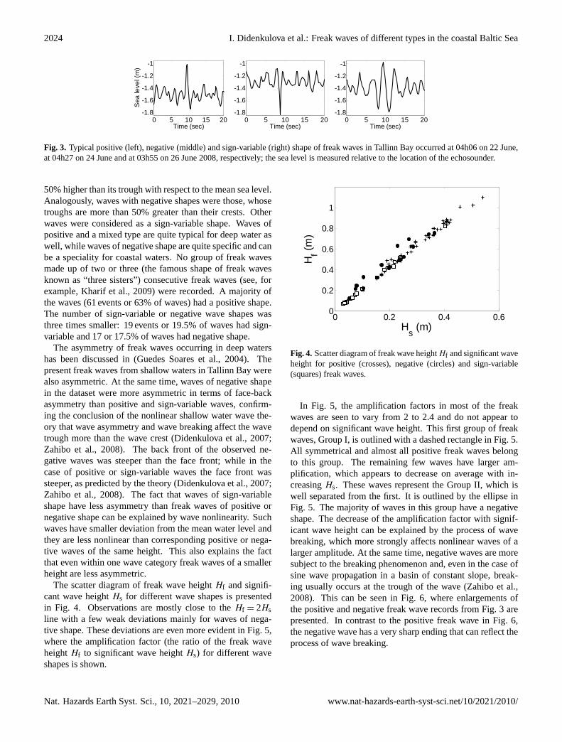
Typical shapes of recorded freak waves are presented inFig. 3. All 97 of the freak waves were solitary waves of a pos-itive, negative or sign-variable shape. The positive shape wasdefined as the shape of the wave, whose crest is more than

www.nat-hazards-earth-syst-sci.net/10/2021/2010/ Nat. Hazards Earth Syst. Sci., 10, 2021–2029, 2010


0 5 10 15 20-1.8

-1.6

-1.4

-1.2

-1

Time (sec)S

ea le

vel (

m)

0 5 10 15 20-1.8

-1.6

-1.4

-1.2

-1

Time (sec)0 5 10 15 20

-1.8

-1.6

-1.4

-1.2

-1

Time (sec) Figure 3. Typical positive (left), negative (middle) and sign-variable (right) shape of freak waves

in Tallinn bay occurred at 4:06 on 22 June, at 4:27 on 24 June and at 3:55 on 26 June 2008

respectively; the sea level is measured relative to the location of the echosounder.

18

Fig. 3. Typical positive (left), negative (middle) and sign-variable (right) shape of freak waves in Tallinn Bay occurred at 04h06 on 22 June,at 04h27 on 24 June and at 03h55 on 26 June 2008, respectively; the sea level is measured relative to the location of the echosounder.

50% higher than its trough with respect to the mean sea level.Analogously, waves with negative shapes were those, whosetroughs are more than 50% greater than their crests. Otherwaves were considered as a sign-variable shape. Waves ofpositive and a mixed type are quite typical for deep water aswell, while waves of negative shape are quite specific and canbe a speciality for coastal waters. No group of freak wavesmade up of two or three (the famous shape of freak wavesknown as “three sisters”) consecutive freak waves (see, forexample, Kharif et al., 2009) were recorded. A majority ofthe waves (61 events or 63% of waves) had a positive shape.The number of sign-variable or negative wave shapes wasthree times smaller: 19 events or 19.5% of waves had sign-variable and 17 or 17.5% of waves had negative shape.

The asymmetry of freak waves occurring in deep watershas been discussed in (Guedes Soares et al., 2004). Thepresent freak waves from shallow waters in Tallinn Bay werealso asymmetric. At the same time, waves of negative shapein the dataset were more asymmetric in terms of face-backasymmetry than positive and sign-variable waves, confirm-ing the conclusion of the nonlinear shallow water wave the-ory that wave asymmetry and wave breaking affect the wavetrough more than the wave crest (Didenkulova et al., 2007;Zahibo et al., 2008). The back front of the observed ne-gative waves was steeper than the face front; while in thecase of positive or sign-variable waves the face front wassteeper, as predicted by the theory (Didenkulova et al., 2007;Zahibo et al., 2008). The fact that waves of sign-variableshape have less asymmetry than freak waves of positive ornegative shape can be explained by wave nonlinearity. Suchwaves have smaller deviation from the mean water level andthey are less nonlinear than corresponding positive or nega-tive waves of the same height. This also explains the factthat even within one wave category freak waves of a smallerheight are less asymmetric.

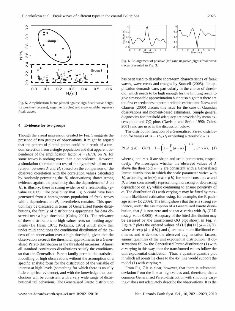
The scatter diagram of freak wave heightHf and signifi-cant wave heightHs for different wave shapes is presentedin Fig. 4. Observations are mostly close to theHf = 2Hsline with a few weak deviations mainly for waves of nega-tive shape. These deviations are even more evident in Fig. 5,where the amplification factor (the ratio of the freak waveheightHf to significant wave heightHs) for different waveshapes is shown.

0 0.2 0.4 0.60

0.2

0.4

0.6

0.8

1

Hs (m)

Hf (m

)

Figure 4. Scatter diagram of freak wave height and significant wave height for positive

(crosses), negative (circles) and sign-variable (squares) freak waves.

fH sH

19

Fig. 4. Scatter diagram of freak wave heightHf and significant waveheight for positive (crosses), negative (circles) and sign-variable(squares) freak waves.

In Fig. 5, the amplification factors in most of the freakwaves are seen to vary from 2 to 2.4 and do not appear todepend on significant wave height. This first group of freakwaves, Group I, is outlined with a dashed rectangle in Fig. 5.All symmetrical and almost all positive freak waves belongto this group. The remaining few waves have larger am-plification, which appears to decrease on average with in-creasingHs. These waves represent the Group II, which iswell separated from the first. It is outlined by the ellipse inFig. 5. The majority of waves in this group have a negativeshape. The decrease of the amplification factor with signif-icant wave height can be explained by the process of wavebreaking, which more strongly affects nonlinear waves of alarger amplitude. At the same time, negative waves are moresubject to the breaking phenomenon and, even in the case ofsine wave propagation in a basin of constant slope, break-ing usually occurs at the trough of the wave (Zahibo et al.,2008). This can be seen in Fig. 6, where enlargements ofthe positive and negative freak wave records from Fig. 3 arepresented. In contrast to the positive freak wave in Fig. 6,the negative wave has a very sharp ending that can reflect theprocess of wave breaking.



0.0 0.1 0.2 0.3 0.4 0.5 0.6

2.0

2.2

2.4

2.6

2.8

3.0

3.2

Hs(m)

Hf

Hs

+ +++

+

+

+ + +++

+

+++

+++++

+ ++++

++ +

+ +

++

+ +

+

+

+

++ ++

++++

++ +

+

+

+

+++ ++

+++++

Group I

Group II

Figure 5. Amplification factor plotted against significant wave height for positive (crosses),

negative (circles) and sign-variable (squares) freak waves.

20

Fig. 5. Amplification factor plotted against significant wave heightfor positive (crosses), negative (circles) and sign-variable (squares)freak waves.

4 Evidence for two groups

Though the visual impression created by Fig. 5 suggests thepresence of two groups of observations, it might be arguedthat the pattern of plotted points could be a result of a ran-dom selection from a single population and that apparent de-pendence of the amplification factorA = Hf/Hs on Hs forsome waves is nothing more than a coincidence. However,a simulation (permutation) test of the hypothesis of no cor-relation betweenA andHs (based on the comparison of theobserved correlation with the correlation values calculatedby randomly permuting theHs observations) shows strongevidence against the possibility that the dependence ofA onHs is illusory; there is strong evidence of a relationship (p-value = 0.013). The possibility that Fig. 5 could have beengenerated from a homogeneous population of freak waveswith a dependence onHs nevertheless remains. This ques-tion may be discussed in terms of Generalised Pareto distri-butions, the family of distributions appropriate for data ob-served over a high threshold (Coles, 2001). The relevanceof these distributions to high values rests on limiting argu-ments (De Haan, 1971; Pickands, 1975) which show thatunder mild conditions the conditional distribution of the ex-cess of an observation over a high threshold, given that theobservation exceeds the threshold, approximates to a Gener-alised Pareto distribution as the threshold increases. Almostall standard continuous distributions satisfy the conditions,so that the Generalised Pareto family permits the statisticalmodelling of high observations without the assumption of aspecific analytic form for the distribution of the variable ofinterest at high levels (something for which there is usuallylittle empirical evidence), and with the knowledge that con-clusions will be consistent with a very wide range of distri-butional tail behaviour. The Generalised Pareto distribution

0 1 2 3 4 5 6 7-1.8

-1.6

-1.4

-1.2

-1

Time (sec)

Sea

leve

l (m

)

0 1 2 3 4 5 6 7-1.8

-1.6

-1.4

-1.2

-1

Time (sec) Figure 6. Enlargement of positive (left) and negative (right) freak wave traces presented in

Figure 3.

21

Fig. 6. Enlargement of positive (left) and negative (right) freak wavetraces presented in Fig. 3.

has been used to describe short-term characteristics of freakwaves, wave crests and troughs by Stansell (2005). Its ap-plication demands care, particularly in the choice of thresh-old, which needs to be high enough for the limiting result togive a reasonable approximation but not so high that there aretoo few exceedances to permit reliable estimation; Naess andClausen (2000) discuss this issue for the case of Gaussianobservations and moment-based estimators. Simple generaldiagnostics for threshold adequacy are provided by mean ex-cess plots and QQ plots (Davison and Smith 1990; Coles,2001) and are used in the discussion below.

The distribution function of a Generalised Pareto distribu-tion for values ofA = Hf/Hs exceeding a thresholdu is

Pr(A ≤ a) = G(a) = 1−

(1+

ξ

σ(a−u)

)−1/ξ

, (a > u), (1)

whereξ andσ > 0 are shape and scale parameters, respec-tively. We investigate whether the observed values ofA

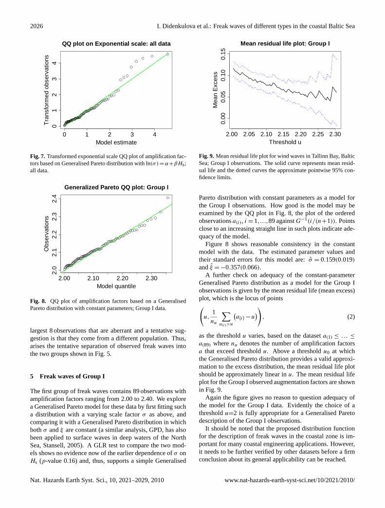
above the thresholdu = 2 are consistent with a GeneralisedPareto distribution in which the scale parameter varies withHs according to ln(σ ) = α +βHs for some constantsα andβ, a form conveniently representing increasing or decreasingdependence onHs whilst continuing to ensure positivity ofσ . The distribution (1) with varyingσ may be fitted by max-imum likelihood estimation using, for example, the R pack-age ismev (R 2009). The fitting shows that there is strong ev-idence, under the assumption of a Generalised Pareto distri-bution, thatβ is non-zero and so thatσ varies withHs (GLRtest;p-value 0.005). Adequacy of the fitted distribution maybe assessed by the transformed QQ plot shown in Fig. 7.Figure 7 plots the ordered values of (1/ξ̂ )ln(1+ξ̂ (a −2)/σ̂ ),whereσ̂=exp (α̂ + β̂Hs) and ξ̂ are maximum likelihood es-timates anda denotes the observed augmentation factors,against quantiles of the unit exponential distribution. If ob-servations follow the Generalised Pareto distribution (1) withσ varying in this way, then the transformed values follow theunit exponential distribution. Thus, a quantile-quantile plotin which all points lie close to the 45◦ line would support themodel (1) with varyingσ .

From Fig. 7 it is clear, however, that there is substantialdeviation from the line at high values and, therefore, that acommon Generalised Pareto distribution with smoothly vary-ing σ does not adequately describe the observations. It is the



0 1 2 3 4

01

23

4

Model estimate

Tran

sfor

med

obs

erva

tions

QQ plot on Exponential scale: all data

Figure 7. Transformed exponential scale QQ plot of amplification factors based on Generalized

Pareto distribution with sHβασ +=)ln( ; all data.

22

Fig. 7. Transformed exponential scale QQ plot of amplification fac-tors based on Generalised Pareto distribution with ln(σ ) = α+βHs;all data.

2.00 2.10 2.20 2.30

2.0

2.1

2.2

2.3

2.4

Model quantile

Obs

erva

tions

Generalized Pareto QQ plot: Group I

Figure 8. QQ plot of amplification factors based on a Generalized Pareto distribution with

constant parameters; Group I data.

23

Fig. 8. QQ plot of amplification factors based on a GeneralisedPareto distribution with constant parameters; Group I data.

largest 8 observations that are aberrant and a tentative sug-gestion is that they come from a different population. Thus,arises the tentative separation of observed freak waves intothe two groups shown in Fig. 5.

5 Freak waves of Group I

The first group of freak waves contains 89 observations withamplification factors ranging from 2.00 to 2.40. We explorea Generalised Pareto model for these data by first fitting sucha distribution with a varying scale factorσ as above, andcomparing it with a Generalised Pareto distribution in whichbothσ andξ are constant (a similar analysis, GPD, has alsobeen applied to surface waves in deep waters of the NorthSea, Stansell, 2005). A GLR test to compare the two mod-els shows no evidence now of the earlier dependence ofσ onHs (p-value 0.16) and, thus, supports a simple Generalised

2.00 2.05 2.10 2.15 2.20 2.25 2.30

0.00

0.05

0.10

0.15

Threshold u

Mea

n Ex

cess

Mean residual life plot: Group I

Figure 9. Mean residual life plot for wind waves in Tallinn Bay, Baltic Sea; Group I

observations. The solid curve represents mean residual life and the dotted curves the

approximate pointwise 95% confidence limits.

24

Fig. 9. Mean residual life plot for wind waves in Tallinn Bay, BalticSea; Group I observations. The solid curve represents mean resid-ual life and the dotted curves the approximate pointwise 95% con-fidence limits.

Pareto distribution with constant parameters as a model forthe Group I observations. How good is the model may beexamined by the QQ plot in Fig. 8, the plot of the orderedobservationsa(i), i = 1,...,89 againstG−1(i/(n+1)). Pointsclose to an increasing straight line in such plots indicate ade-quacy of the model.

Figure 8 shows reasonable consistency in the constantmodel with the data. The estimated parameter values andtheir standard errors for this model are:σ̂ = 0.159(0.019)andξ̂ = −0.357(0.066).

A further check on adequacy of the constant-parameterGeneralised Pareto distribution as a model for the Group Iobservations is given by the mean residual life (mean excess)plot, which is the locus of points(

u,1

nu

∑a(i)>u

(a{i} −u

)), (2)

as the thresholdu varies, based on the dataseta(1) ≤ ... ≤

a(89) wherenu denotes the number of amplification factorsa that exceed thresholdu. Above a thresholdu0 at whichthe Generalised Pareto distribution provides a valid approxi-mation to the excess distribution, the mean residual life plotshould be approximately linear inu. The mean residual lifeplot for the Group I observed augmentation factors are shownin Fig. 9.

Again the figure gives no reason to question adequacy ofthe model for the Group I data. Evidently the choice of athresholdu=2 is fully appropriate for a Generalised Paretodescription of the Group I observations.

It should be noted that the proposed distribution functionfor the description of freak waves in the coastal zone is im-portant for many coastal engineering applications. However,it needs to be further verified by other datasets before a firmconclusion about its general applicability can be reached.



20 25 30 35 40 45 500

5

10

15

Time (day)

Win

d sp

eed

(m/s

)

Figure 10. Wind speed for 20 June-21 July 2008 in Kalbadagrund (Finland); the circles show the

times when freak waves of the Group II occurred.

25

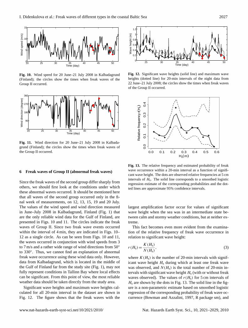
Fig. 10. Wind speed for 20 June–21 July 2008 in Kalbadagrund(Finland); the circles show the times when freak waves of theGroup II occurred.

20 25 30 35 40 45 500

90

180

270

360

Time (day)

Win

d di

rect

ion

(deg

ree)

Figure 11. Wind direction for 20 June-21 July 2008 in Kalbadagrund (Finland); the circles show

the times when freak waves of the Group II occurred.

26

Fig. 11. Wind direction for 20 June–21 July 2008 in Kalbada-grund (Finland); the circles show the times when freak waves ofthe Group II occurred.

6 Freak waves of Group II (abnormal freak waves)

Since the freak waves of the second group differ sharply fromothers, we should first look at the conditions under whichthese abnormal waves occurred. It should be mentioned herethat all waves of the second group occurred only in the fi-nal week of measurements, on 12, 13, 15, 19 and 20 July.The values of the wind speed and wind direction measuredin June–July 2008 in Kalbadagrund, Finland (Fig. 1) thatare the only reliable wind data for the Gulf of Finland, arepresented in Figs. 10 and 11. The circles indicate the freakwaves of Group II. Since two freak wave events occurredwithin the interval of 4 min, they are indicated in Figs. 10–12 as a single circle. As can be seen from Figs. 10 and 11,the waves occurred in conjunction with wind speeds from 3to 7 m/s and a rather wide range of wind directions from 50◦

to 330◦. Thus, we cannot find an explanation of abnormalfreak wave occurrence using these wind data only. However,data from Kalbadagrund, which is located in the middle ofthe Gulf of Finland far from the study site (Fig. 1), may notfully represent conditions in Tallinn Bay where local effectscan be significant. From this point of view, the most reliableweather data should be taken directly from the study area.

Significant wave heights and maximum wave heights cal-culated for all 20-min interval in the dataset are shown inFig. 12. The figure shows that the freak waves with the

25 30 35 40 45 500

0.2

0.4

0.6

0.8

1

1.2

Time (day)

Wav

e he

ight

(m)

Figure 12. Significant wave heights (solid line) and maximum wave heights (dotted line) for 20-

minute intervals of the night data from 22 June-21 July 2008; the circles show the times when

freak waves of the Group II occurred.

27

Fig. 12. Significant wave heights (solid line) and maximum waveheights (dotted line) for 20-min intervals of the night data from22 June–21 July 2008; the circles show the times when freak wavesof the Group II occurred.

0.0 0.1 0.2 0.3 0.4 0.5 0.6

0.0

0.1

0.2

0.3

0.4

Hs(m)

Rel

ativ

e fre

quen

cy r(

Hs)

Figure 13. The relative frequency and estimated probability of freak wave occurrence within a

20-minute interval as a function of significant wave height. Dots are observed relative

frequencies at 5 cm intervals of Hs. The solid line corresponds to a smoothed logistic regression

estimate of the corresponding probabilities, and the dotted lines are approximate 95% confidence

intervals.

28

Fig. 13. The relative frequency and estimated probability of freakwave occurrence within a 20-min interval as a function of signifi-cant wave height. The dots are observed relative frequencies at 5 cmintervals ofHs. The solid line corresponds to a smoothed logisticregression estimate of the corresponding probabilities and the dot-ted lines are approximate 95% confidence intervals.

largest amplification factor occur for values of significantwave height when the sea was in an intermediate state be-tween calm and stormy weather conditions, but at neither ex-treme.

This fact becomes even more evident from the examina-tion of the relative frequency of freak wave occurrence inrelation to significant wave height:

r (Hs) =K(Hs)

N (Hs), (3)

whereK(Hs) is the number of 20-min intervals with signif-icant wave heightHs during which at least one freak wavewas observed, andN(Hs) is the total number of 20-min in-tervals with significant wave heightHs (with or without freakwaves observed). The values ofr(Hs) for 5 cm intervals ofHs are shown by the dots in Fig. 13. The solid line in the fig-ure is a non-parametric estimate based on smoothed logisticregression of the corresponding probability of freak wave oc-currence (Bowman and Azzalini, 1997, R package sm), and



Figure 14. Time-frequency spectrum (extracts 60 sec) of the record of 13 July 2008; shades of

grey indicate the spectral density; dashed lines correspond to the time of the freak wave

occurrence; the ellipse corresponds to the dispersive track.

29

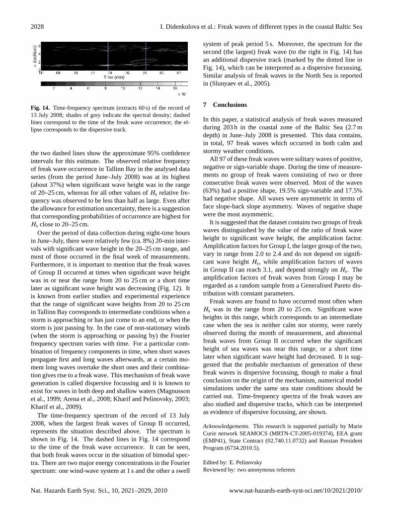
Fig. 14. Time-frequency spectrum (extracts 60 s) of the record of13 July 2008; shades of grey indicate the spectral density; dashedlines correspond to the time of the freak wave occurrence; the el-lipse corresponds to the dispersive track.

the two dashed lines show the approximate 95% confidenceintervals for this estimate. The observed relative frequencyof freak wave occurrence in Tallinn Bay in the analysed dataseries (from the period June–July 2008) was at its highest(about 37%) when significant wave height was in the rangeof 20–25 cm, whereas for all other values ofHs relative fre-quency was observed to be less than half as large. Even afterthe allowance for estimation uncertainty, there is a suggestionthat corresponding probabilities of occurrence are highest forHs close to 20–25 cm.

Over the period of data collection during night-time hoursin June–July, there were relatively few (ca. 8%) 20-min inter-vals with significant wave height in the 20–25 cm range, andmost of those occurred in the final week of measurements.Furthermore, it is important to mention that the freak wavesof Group II occurred at times when significant wave heightwas in or near the range from 20 to 25 cm or a short timelater as significant wave height was decreasing (Fig. 12). Itis known from earlier studies and experimental experiencethat the range of significant wave heights from 20 to 25 cmin Tallinn Bay corresponds to intermediate conditions when astorm is approaching or has just come to an end, or when thestorm is just passing by. In the case of non-stationary winds(when the storm is approaching or passing by) the Fourierfrequency spectrum varies with time. For a particular com-bination of frequency components in time, when short wavespropagate first and long waves afterwards, at a certain mo-ment long waves overtake the short ones and their combina-tion gives rise to a freak wave. This mechanism of freak wavegeneration is called dispersive focussing and it is known toexist for waves in both deep and shallow waters (Magnussonet al., 1999; Arena et al., 2008; Kharif and Pelinovsky, 2003;Kharif et al., 2009).

The time-frequency spectrum of the record of 13 July2008, when the largest freak waves of Group II occurred,represents the situation described above. The spectrum isshown in Fig. 14. The dashed lines in Fig. 14 correspondto the time of the freak wave occurrence. It can be seen,that both freak waves occur in the situation of bimodal spec-tra. There are two major energy concentrations in the Fourierspectrum: one wind-wave system at 1 s and the other a swell

system of peak period 5 s. Moreover, the spectrum for thesecond (the largest) freak wave (to the right in Fig. 14) hasan additional dispersive track (marked by the dotted line inFig. 14), which can be interpreted as a dispersive focussing.Similar analysis of freak waves in the North Sea is reportedin (Slunyaev et al., 2005).

7 Conclusions

In this paper, a statistical analysis of freak waves measuredduring 203 h in the coastal zone of the Baltic Sea (2.7 mdepth) in June–July 2008 is presented. This data contains,in total, 97 freak waves which occurred in both calm andstormy weather conditions.

All 97 of these freak waves were solitary waves of positive,negative or sign-variable shape. During the time of measure-ments no group of freak waves consisting of two or threeconsecutive freak waves were observed. Most of the waves(63%) had a positive shape, 19.5% sign-variable and 17.5%had negative shape. All waves were asymmetric in terms offace slope-back slope asymmetry. Waves of negative shapewere the most asymmetric.

It is suggested that the dataset contains two groups of freakwaves distinguished by the value of the ratio of freak waveheight to significant wave height, the amplification factor.Amplification factors for Group I, the larger group of the two,vary in range from 2.0 to 2.4 and do not depend on signifi-cant wave heightHs, while amplification factors of wavesin Group II can reach 3.1, and depend strongly onHs. Theamplification factors of freak waves from Group I may beregarded as a random sample from a Generalised Pareto dis-tribution with constant parameters.

Freak waves are found to have occurred most often whenHs was in the range from 20 to 25 cm. Significant waveheights in this range, which corresponds to an intermediatecase when the sea is neither calm nor stormy, were rarelyobserved during the month of measurement, and abnormalfreak waves from Group II occurred when the significantheight of sea waves was near this range, or a short timelater when significant wave height had decreased. It is sug-gested that the probable mechanism of generation of thesefreak waves is dispersive focussing, though to make a finalconclusion on the origin of the mechanism, numerical modelsimulations under the same sea state conditions should becarried out. Time-frequency spectra of the freak waves arealso studied and dispersive tracks, which can be interpretedas evidence of dispersive focussing, are shown.

Acknowledgements.This research is supported partially by MarieCurie network SEAMOCS (MRTN-CT-2005-019374), EEA grant(EMP41), State Contract (02.740.11.0732) and Russian PresidentProgram (6734.2010.5).

Edited by: E. PelinovskyReviewed by: two anonymous referees



References

Al-Humoud, J., Tayfun, M. A., and Askar, H.: Distribution of non-linear wave crests, Ocean Eng., 29, 1929–1943, 2002.

Arena, F., Ascanelli, A., Nava, V., Pavone, D., and Romolo, A.:Three-dimensional nonlinear random wave groups in intermedi-ate water depth, Coastal Eng., 55, 1052–1061, 2008.

Bitner, E. M.: Nonlinear effects of the statistical model of shallow-water wind-waves, Appl. Ocean Res., 2, 63–73, 1980.

Bitner-Gregersen, E. M. and Magnusson, A. K.: Extreme events infield data and in a second order wave model, Proc. Rogue Waves2004, Brest, France, 2004.

Bowman, A. W. and Azzalini, A.: Applied Smoothing Techniquesfor Data Analysis: the Kernel Approach with S-Plus Illustrations,Oxford University Press, Oxford, 1997.

Caliskan, H. and Valle-Levinson, A.: Wind-wave transformationsin an elongated bay, Cont. Shelf Res., 28, 1702–1710, 2008.

Cherneva, Z., Petrova, P., Andreeva, N., and Guedes Soares, C.:Probability distributions of peaks, troughs and heights of wind-waves measured in the black sea coastal zone, Coastal Eng., 52,599–615, 2005.

Chien, H., Kao, C.-C., and Chuang, L. Z. H.: On the characteristicsof observed coastal freak waves, Coastal Eng. J., 44(4), 301–319,2002.

Coles, S.: An introduction to statistical modelling of extreme val-ues, Springer, Berlin, 2001.

Davison, A. C.and Smith, R. L.: Models for exceedances over highthresholds (with discussion), J. Roy. Stat. Soc. B, 52, 393–442,1990.

Dean, R. G. and Dalrymple, R. A.: Coastal processes with engineer-ing applications, Cambridge University Press, Cambridge, 2002.

De Haan, L.: On regular variation and its application to the weakconvergence of sample extremes, Mathematical Center Tracts,Amsterdam, 1971.

Didenkulova, I., Pelinovsky, E., Soomere, T., and Zahibo, N.:Runup of nonlinear asymmetric waves on a plane beach, in:Tsunami and Nonlinear Waves, edited by: Kundu, A., Springer,173–188, 2007.

Didenkulova, I. I., Slunyaev, A. V., Pelinovsky, E. N., and Kharif,C.: Freak waves in 2005, Nat. Hazards Earth Syst. Sci., 6, 1007–1015, doi:10.5194/nhess-6-1007-2006, 2006.

Glukovskij, B. Ch.: Research of Wind Waves, Hydrometeor. Publ.,Leningrad, 1966.

Guedes Soares, C., Cherneva, Z., and Antao, E. M.: Steepness andasymmetry of the largest waves in storm sea states, Ocean Eng.,31, 1147–1167, 2003.

Kask, J., Talpas, A., Kask, A., and Schwarzer, K.: Geological set-ting of areas endangered by waves generated by fast ferries inTallinn Bay, Estonian Journal of Engineering, 9, 185–208, 2003.

Kharif, Ch. and Pelinovsky, E.: Physical mechanisms of the roguewave phenomenon, Eur. J. Mech. B-Fluid., 22, 603–634, 2003.

Kharif, Ch., Pelinovsky, E., and Slunyaev, A.: Rogue waves in theocean, Springer, 2009.

Krogstad, K. E., Barstow, S. F., Mathisen, J. P., Lønseth, L., Mag-nusson, A. K., and Donelan, M. A.: Extreme Waves in the Long-Term Wave Measurements at Ekofisk, Proc. Rogue Waves 2008Workshop, Brest, France, 13–15 October 2008.

Lutt, J. and Tammik, P.: Bottom sediments of Tallinn Bay, EstonianJournal of Earth Sciences, 41, 81–87, 1992.

Magnusson, A. K., Donelan, M. A., and Drennan, W. M.: On es-timating extremes in an evolving wave field, Coastal Eng., 36,147–163, 1999.

Massel, S. R.: Hydrodynamics of coastal zones, Elsevier, Amster-dam, 1989.

Massel, S. R.: Ocean surface waves: their physics and prediction,World Scientific Publ., Singapore, 1996.

Mori, N. and Yasuda, T.: A weakly non-gaussian model of waveheight distribution for random wave train, Ocean Eng., 29, 1219–1231, 2002.

Neelamani, S., Al-Salem, K., and Rakha, K.: Extreme waves forKuwaiti territorial waters, Ocean Eng., 34, 1496–1504, 2007.

Olagnon, M.: About the frequency of occurrence of rogue waves,Proceedings of the Rogue Waves 2008 Workshop, Brest, France,13–15 October 2008.

Petrova, P., Cherneva, Z., and Guedes Soares, C.: Distribution ofcrest heights in sea states with abnormal waves, Appl. OceanRes., 28, 235–245, 2006.

Pickands, J.: Statistical inference using extreme order statistics,Ann. Stat., 3, 119–131, 1971.

Prevosto, M., Krogstad, H. E., and Robin, A.: Probability distri-butions for maximum wave and crest heights, Coastal Eng., 40,329–360, 2000.

R Development Core Team: R: A language and environment for sta-tistical computing, reference index version 2.10.0, R Foundationfor Statistical Computing, Vienna, Austria, 2009.

Slunyaev, A., Pelinovsky, E., and Guedes Soares, C: Modeling freakwaves from the North Sea, Appl. Ocean Res., 27, 12–22, 2005.

Soomere, T., Behrens, A., Tuomi, L., and Nielsen, J. W.: Waveconditions in the Baltic Proper and in the Gulf of Finland dur-ing windstorm Gudrun, Nat. Hazards Earth Syst. Sci., 8, 37–46,doi:10.5194/nhess-8-37-2008, 2008.

Soomere, T.: Wind wave statistics in Tallinn Bay, Boreal Environ.Res., 10, 103–118, 2005.

Stansell, P.: Distributions of extreme wave, crest and trough heightsmeasured in the North Sea, Ocean Eng., 32, 1015–1036, 2005.

Toffoli, A., Lefevre, J. M., Bitner-Gregersen, E., and Monbaliu, J.:Towards the identification of warning criteria: analysis of a shipaccident database, Appl. Ocean Res., 27, 281–291, 2005.

Walker, D. A. G., Taylor, P. H., and Eatock Taylor, R.: The shape oflarge surface waves on the open sea and the Draupner New Yearwave, Appl. Ocean Res., 26, 73–83, 2004.

Young, I. R. and Babanin, A. V.: The form of the asymptotic depth-limited wind-wave spectrum. Part II – The wavenumber spec-trum, Coastal Eng., 56, 534–542, 209.

Zahibo, N., Didenkulova, I., Kurkin, A., and Pelinovsky, E.: Steep-ness and spectrum of nonlinear deformed shallow water wave,Ocean Eng., 35, 47–52, 2008.


Documents

nhess-10-2021-2010 Didenkulova Anderson