NITA’s mobile LRAIC model - Erhvervsstyrelsen · NITA’s mobile LRAIC model ... HLR dimensioning w excluded from the traffic- ... w equivalent to 4 CE 6. Data demand drivers

NITA’s mobile LRAIC model

Summary of the draft demand and network model for all parties

Copenhagen, 30 and 31 August 2007

2

Agenda

Activities and timetable

Draft demand and network model – industry summary

Operator-specific models

Next steps

3

Current activities

� Analysys has produced the first version of the LRAIC model

w to be distributed to industry parties as the first of three consultations on the model

� NITA will release the model to the industry parties on 3 September, at the start of the hearing process

� NITA has also published accompanying conclusions on the model specification consultation

� Analysys will commence work on the next phase of data review (top-down data and/or top-down models)

4

The timetable has been revised to accommodate additional industry interaction

5


Operators have eightweeks with the draft demand and network

model

6


Top-down cost data is due next week, top-

down models by 1 October 2007

7


We are due back in Copenhagen in six weeks’ time to:

(1) Review top-down submissions (2) Discuss the model consultation with each operator

8


We will bring together:

(1) Draft demand and network model(2) Operator responses(3) Cost data submissions(4) A possible further visit to Copenhagen

… and respond with a revised draft (the ‘draft cost model’) by Christmas

9




Next steps

10

Summary of the draft demand and network model for all industry parties

� We are presenting this summary and discussion to all of the mobile operators

w it may also be made public by NITA, distributed to MVNOs, etc.

� An operator-specific annex containing confidential parameters and model outputs will follow for each of the four mobile network operators

w we have not developed an MVNO version yet, although will be working on one in the coming few weeks. This version is likely to utilise only a few network assets

11

Sequence of model components

1. Subscribers

2. Voice traffic

3. Data traffic

4. Operator share

5. Voice demand drivers

6. Data demand drivers

7. Element interactions

8. Coverage drivers

9. Network roll-out

10. Radio network

11. Backhaul network

12. BSC and BSC-MSC

13. MSC, TSC, HLR

14. Backbone network

15. SMSC, GSNs

16. Expenditure rules

17. Unit costs

18. Incremental costs

12

We forecast mobile penetration based on the level at the end of 2006

� Registered plus hosted subscribers amount to 6.2 million subscribers – 115% penetration

� Long-term penetration is accordingly forecast at 120%

� In addition, a number of ‘non-personal’ SIMs are:

w included in the model for HLR dimensioning

w excluded from the traffic-per-subscriber calculations 0%

20%

40%

60%

80%

100%

120%

140%

1992

1994

1996

1998

2000

2002

2004

2006

2008

2010

2012

2014

SIM

pen

etra

tion

1. Subscribers

Personal mobile penetration

Source: NITA, operator data, Analysys

13

The total number of SIMs increases to over 7 million in the long term

� The forecast of SIM penetration is relatively static given recent growth in subscriber numbers

� The eventual penetration level is highly debatable, and depends upon:

w definition of ‘active’ subscribers

w the number of dual-SIM and dual-operator individuals

w non-personal SIMs (cabin control and industrial)

0

1

2

3

4

5

6

7

1992

1994

1996

1998

2000

2002

2004

2006

2008

2010

2012

2014

Yea

r end

sub

scrib

ers

(mill

ions

)

Registered/hosted Non-personal SIMsNational population

1. Subscribers

Subscription levels

Source: NITA, operator data, Analysys

14

The model includes the option to migrate from 2G to 3G, and from 3G

� Established operators exhibit approximately 1% migration to 3G at end 2006

� A migration profile is defined in the model – applicable to both 2G and 3G

� The profile results in a 2G shut-down date of 2012 (2013 for Telia)

� There is also the option of a 3G shut-down date of 2023

1. Subscribers

Migration profile

Source: Analysys

0

10

20

30

40

50

60

70

80

90

100

1 2 3 4 5 6 7 8

Year

Mig

ratio

n pr

ofile

(%)

15

Voice traffic is calculated on a usage-per-subscriber basis, forecast for each operator

� The model contains an indicative medium-usage growth forecast

w projected from actual 2006 values for each operator

� The rapid growth in usage from 2004 to 2006 stands out as a recent phenomenon

� Additional scenarios can easily be added to the model by duplicating the scenario sheet and referencing the sheet name (in the control panel)

2. Voice traffic

0

5

10

15

20

25

1992

1995

1998

2001

2004

2007

2010

2013

2016

2019

2022

Min

utes

(bill

ions

)2G outgoing, on-net, VMS minutes3G outgoing, on-net, VMS minutes2G incoming minutes3G incoming minutes

Total ‘medium-growth’ voice usage, including migration

Source: model input data, Analysys

16

Data usage is forecast in a similar way: per-subscriber, operator-specific, medium-growth

� Data traffic statistics are:

� Year 2006

w SMS 17 billion

w PS data 40 000 GB

w Video 5 million mins

� Year 2018 peak

w SMS 41 billion

w PS data 460 000 GB

w Video 70 million mins

0

50

100

150

200

250

300

350

400

450

500

1992

1995

1998

2001

2004

2007

2010

2013

2016

2019

2022

Vid

eo, p

acke

t dat

a

0

5

10

15

20

25

30

35

40

45

SM

S m

essa

ges

2G packet data (terabytes)3G packet data (Release 99) (terabytes)3G video (million minutes)2G SMS messages (billion)3G SMS messages (billion)

3. Data traffic

Total ‘medium-growth’ data usage, including migration

Source: model input data, Analysys

17

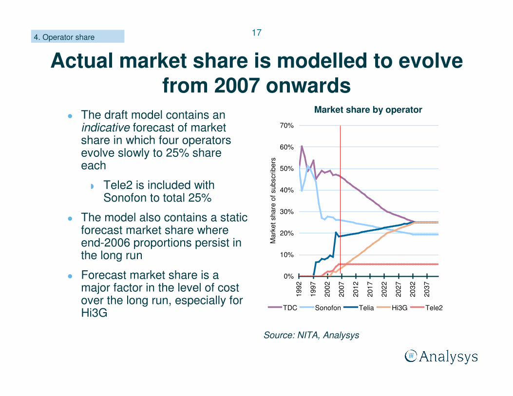
Actual market share is modelled to evolve from 2007 onwards

� The draft model contains an indicative forecast of market share in which four operators evolve slowly to 25% share each

w Tele2 is included with Sonofon to total 25%

� The model also contains a static forecast market share where end-2006 proportions persist in the long run

� Forecast market share is a major factor in the level of cost over the long run, especially for Hi3G

4. Operator share

Market share by operator

Source: NITA, Analysys

0%

10%

20%

30%

40%

50%

60%

70%

1992

1997

2002

2007

2012

2017

2022

2027

2032

2037

Mar

ket s

hare

of s

ubsc

riber

s

TDC Sonofon Telia Hi3G Tele2

18

The voice volume is converted to busy-hour load, according to operator characteristics

� The following parameters are inputs to the model, by operator

w proportion of traffic in weekdays (250 busy days per year)

w proportion of weekday traffic in busy hour

w average call duration

w call attempts per call

� Used to calculate busy-hour Erlang (BHE) and busy-hourcall attempts (BHCA) by service

5. Voice demand drivers

1.15Call attempts per call

30 secondsCall duration (to VMS)

1 ¾ minutesCall duration (to end user)

8%Busy-hour percentage

80%Weekday traffic proportion

Approximate average

Parameter

Source: operator data, Analysys estimates

19

Additional parameters and inputs are used to determine the peak data traffic drivers

� Busy days per year either weekdays (250) or weekends (115)

� SMS-specific busy-day and busy-hour percentages

� Cost allocation considers equivalence of 1150 SMS per minute, based on:

w 8×SDCCH channel per TCH

w 40 bytes per SMS

� Same busy-hour profile as voice

� 64kbit/s symmetric and guaranteed service

w equivalent to 4 CE

6. Data demand drivers

� Same busy-hour profile as voice

� Uplink/downlink proportion is assumed to be symmetric on average, e.g. MMS messaging is highly asymmetric per leg, but symmetric on average

� +12% IP overheads

� Cost allocation considers effective channel rate:

� GPRS 13.4kbit/s CS2

� Rel-99 3G 16kbit/s

SMS Packet data Video

20

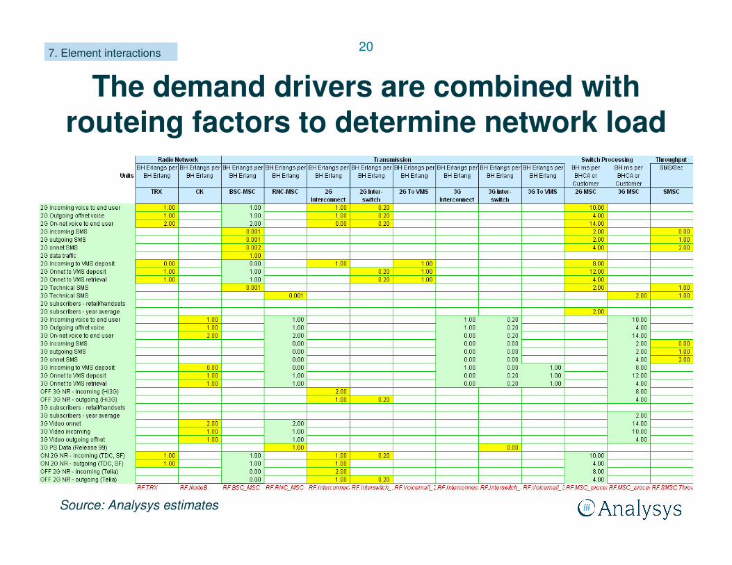
The demand drivers are combined with routeing factors to determine network load


Source: Analysys estimates

21



1:1:2 rule for in:out:on-net traffic

zero when the VMS answers the call

one for on-network national roaming legs (carried by TDC and Sonofon)

2G SMS and 2G packet data assumed to be carried in dedicated channel reservations

3G SMS assumed to be carried in signalling reservation

3G packet data has a scenario for adding to 3G radio load


22



All traffic on the radio network must travel from the BSC/RNC to the main switching

centres on transmission capacity


23



Interconnected traffic:incoming, outgoing off-net,

national roaming voice

Inter-switch traffic: an estimated/measured proportion of incoming,

outgoing and on-net voice

VMS traffic:deposits and retrievals

Same for 2G and 3G


24



Switch processing (BHms per CA):

Incoming = 10, Outgoing = 4, On-net = 4+10

SMS message = 2 per leg

Answered by VMS = -2

Location updates = 2 per handset

National roaming traffic also switched by both parties (off-network like VMS diverted)

Same for 2G and 3G

Outgoing/on-net SMS also handled by SMSCSource: Analysys estimates

25

NITA’s mast database, with operator data, has been used to specify details of coverage

� All operators recognise approximately 95% of Denmark as ‘rural’

w the main differences occur in the number and size of urban geotypes

� We have averaged across operator data and used the mast database to identify sites by geotype for each operator

8. Coverage drivers

Dense urban

Urban

Suburban

Rural

Dense urban

Urban

Suburban

Rural

4094495.75%Rural

14303.34%Suburban

3500.82%Urban

400.09%Dense urban

Size (sq. km)AreaGeotype

Source: operator data, Analysys

26

The mast database has some limitations, but is invaluable for coverage modelling

� Limitations include missing data points (which we have managed to resolve through post-processing of the database) and BTS start dates (which is inconsistent with the spectrum allocation)

� However, we have calibrated the theoretical radius of outdoor coverage using the mast database and operator data, and hexagonal modelling in MapInfo

8. Coverage drivers

MapInfo model of hexagonal outdoor coverage at each BTS

Source: operator data, NITA, Analysys

27

Theoretical coverage cell radii

� The hexagonal model of coverage used in MapInfo defines the theoretical outdoor coverage that can be achieved from each site, by geotype

� Operators provided outdoor coverage data (over time) to calibrate the hexagonal mapping model

� Cell radii:

w decrease with clutter

w decrease with frequency

8. Coverage drivers

Calibrated cell radii for outdoor coverage

Source: Analysys

0

1

2

3

4

5

6

7

8

9

10

Denseurban

Urban Suburban Rural

Theo

retic

al ra

dius

(km

)

900MHz 1800MHz 2100MHz

28

We have captured the difference between optimal and scorched-node radio coverage

� In an optimal, greenfield network, coverage would be achieved with the theoretical cell radius

� In reality, operators are constrained in the potential locations for BTSs, and must take a strategic decision about how well they fill the resulting gaps (by frequency)

� The ratio of the effective to theoretical coverage per site is the ‘scorched-node coverage coefficient’ and is always less than 1.00

8. Coverage drivers

Optimal locations of BTS

Sub-optimal locations of BTS

occurring in reality

Coverage models

Source: Analysys

29

The model rolls out separate 900MHz, 1800MHz and 3G-2100MHz networks

� The relevant model input is by three dimensions:

w by geotype

w by frequency

w by time (history + forecast)

� Historical coverage by operator is estimated or calculated from the mast database and operator data, using MapInfo

� Special site (indoor, tunnel) roll-out is also specified

� Coverage profiles are provided in the confidential annexes

9. Network roll-out

30

Site deployments for coverage

� The primary spectrum used for coverage is defined for each operator (900MHz for TDC and Sonofon, 1800MHz for Telia, 2100MHz for Hi3G)

� Secondary spectrum coverage BTSs are deployed mainly on existing primary spectrum sites

w although some variation exists by operator/geotype

� 3G coverage deployed mainly on existing 2G sites

w although some variation exists by operator/geotype

� Deployment is predominantly tri-sectored to maximise coverage (some 1- and 2-sector deployments in rural areas with 900MHz)

10. Radio network

31

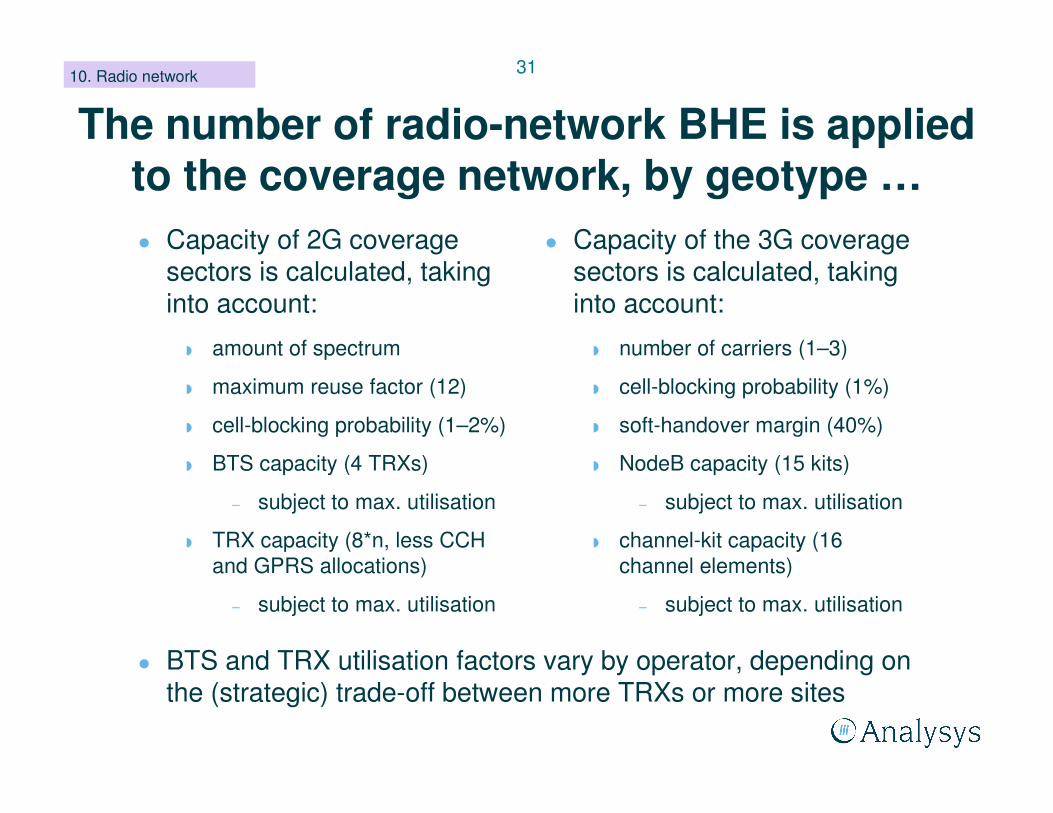
The number of radio-network BHE is applied to the coverage network, by geotype …� Capacity of 2G coverage

sectors is calculated, taking into account:

w amount of spectrum

w maximum reuse factor (12)

w cell-blocking probability (1–2%)

w BTS capacity (4 TRXs)

– subject to max. utilisation

w TRX capacity (8*n, less CCH and GPRS allocations)


� Capacity of the 3G coverage sectors is calculated, taking into account:

w number of carriers (1–3)

w cell-blocking probability (1%)

w soft-handover margin (40%)

w NodeB capacity (15 kits)


w channel-kit capacity (16 channel elements)


10. Radio network

� BTS and TRX utilisation factors vary by operator, depending on the (strategic) trade-off between more TRXs or more sites

32

…and BHEs that cannot be supported by coverage sites require additional BTSs� The additional BTS deployed:

w are always tri-sectored

w utilise primary and/or secondary spectrum in a certain (average) proportion by geotype

– these proportions vary by operator

10. Radio network

33

Other radio network elements are dimensioned more straightforwardly

� A proportion of traffic (approx. 1%) is carried on special sites (indoor and tunnel sites). These are deployed with a fixed number of TRXs or CKs per site

w i.e. capacity elements not driven explicitly by traffic

� Site types are deployed according to a percentage input

10. Radio network

Own tower site Third-party tower site Third-party rooftop site

(blue shading denotes own equipment; grey shading denotes third-party assets)

Own monopole site

Source: Analysys

34

Separate 2G and 3G backhaul transmission is modelled using the same logical structure

� The backhaul requirement per site is calculated as n E1 units per site, based on channels at the BTS, plus a maximum utilisation factor

� A proportion of sites therefore use n E1 leased lines per site

� Remaining sites use part-filled 8Mbit/s microwave

� A proportion of (rural) sites are connected to an access node on the fibre backbone (ratio of 9 sites per node)

� Special sites just use 1×E1

11. Backhaul network

Backhaul network elements

BSC

8Mbit/s microwave (nE1 part-

filled)

AN

Special sites

n E1 leased lines per site on average

E1

E1 E1

Up to 9 BTS per

AN

Fibre backbone

1××××E1

Source: Analysys

35

BSC and RNC switches are dimensioned using radio network parameters

� BSC switches are dimensioned on the basis of:

w TRX capacity

w maximum utilisation

� A proportion of BSCs are modelled to be remote from MSCs

� The average traffic passing through these BSCs is carried on E1 links, provisioned on the fibre backbone

� RNC switches are dimensioned on the basis of:

w NodeB capacity

w Mbit/s throughput

w maximum utilisation

� Again, a proportion can be remote from the MSC layer

� Again, the average traffic passing through these RNCsis carried on E1 links, provisioned on the fibre backbone

12. BSC and BSC–MSC

36

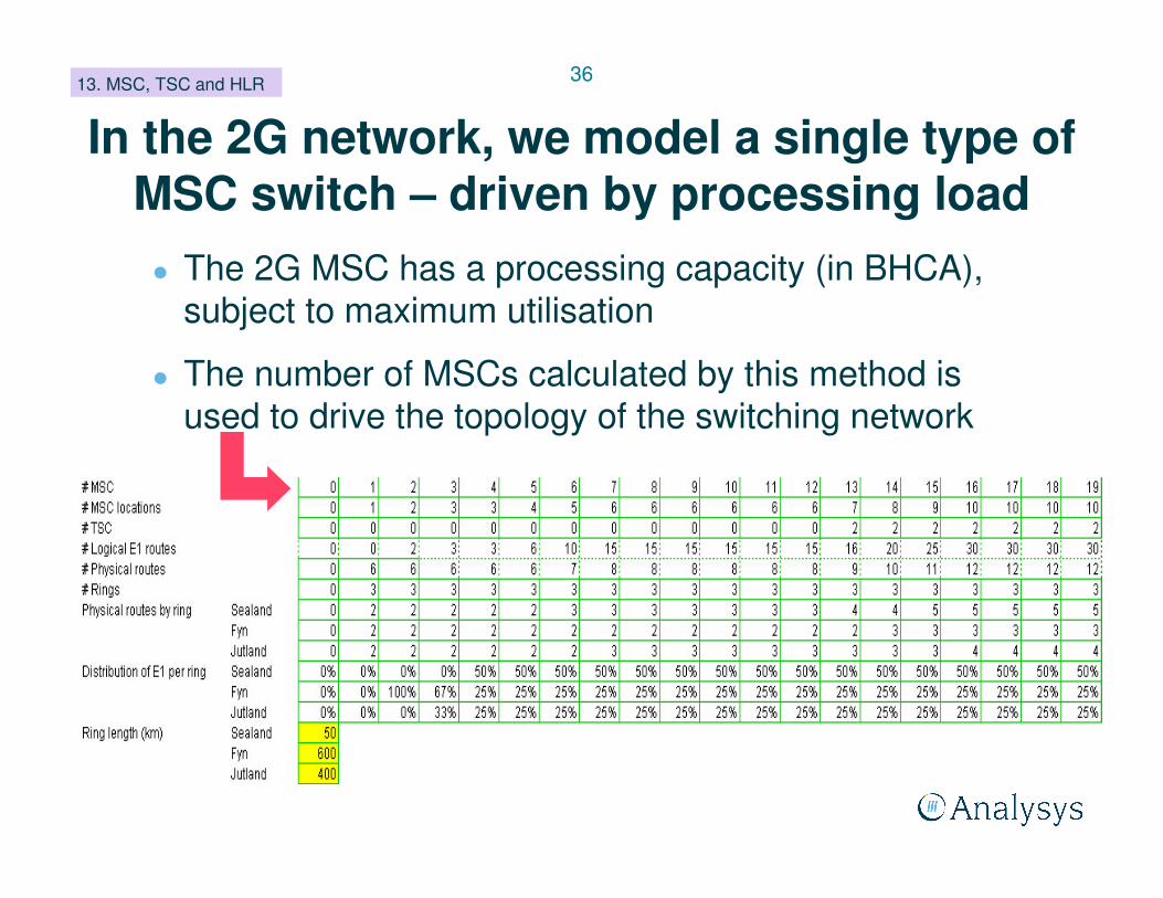
In the 2G network, we model a single type of MSC switch – driven by processing load� The 2G MSC has a processing capacity (in BHCA),

subject to maximum utilisation

� The number of MSCs calculated by this method is used to drive the topology of the switching network

13. MSC, TSC and HLR

37

In the 3G network, the MSC layer is modelled with two types of switch: server and gateway


Mobile switching server (MSS) Media gateway (MGW)

3G BHCAsMSS processor maximum utilisation

MSS processor capacity Number of MSSs

Switching topologySwitching topology look-up table

Traffic per route

E1 ports

BHE on inter-switch, interconnect, VMS

MGW port maximum utilisation

MGW port capacity

Number of MGWs

Source: Analysys

38

HLR units are driven by registered personal and non-personal SIMs

� The capacity per HLR unit, plus maximum utilisation is used to calculate HLR units over time

� 2G and 3G subscribers are combined in the HLR


39

Up to 12 MSC or 6 locations, a fully-meshed inter-MSC network is modelled

� Mature GSM networks are typically beyond 3 sites, however evolving 3G networks have yet to reach the same extent ( denotes a switching location)

1

2

1

2

3

1

2

3

45

6

6 logical routes

10 logical routes

15 logical routes

0 logical routes

2 logical routes

3 logical routes


Source: Analysys

40

For 12 MSCs and 7 locations, a two-mesh transit layer is deployed

� As the number of MSC locations increases, it becomes more efficient to deploy transit nodes

� Transit switches are assumed to not be necessary in the 3G network

w 3G switches are much larger in capacity than historical 2G switches

MSC locationTSC

6 logical routes 10 logical routes

7 locationsm

esh 1

mesh 2

Transit topology


Source: Analysys

41

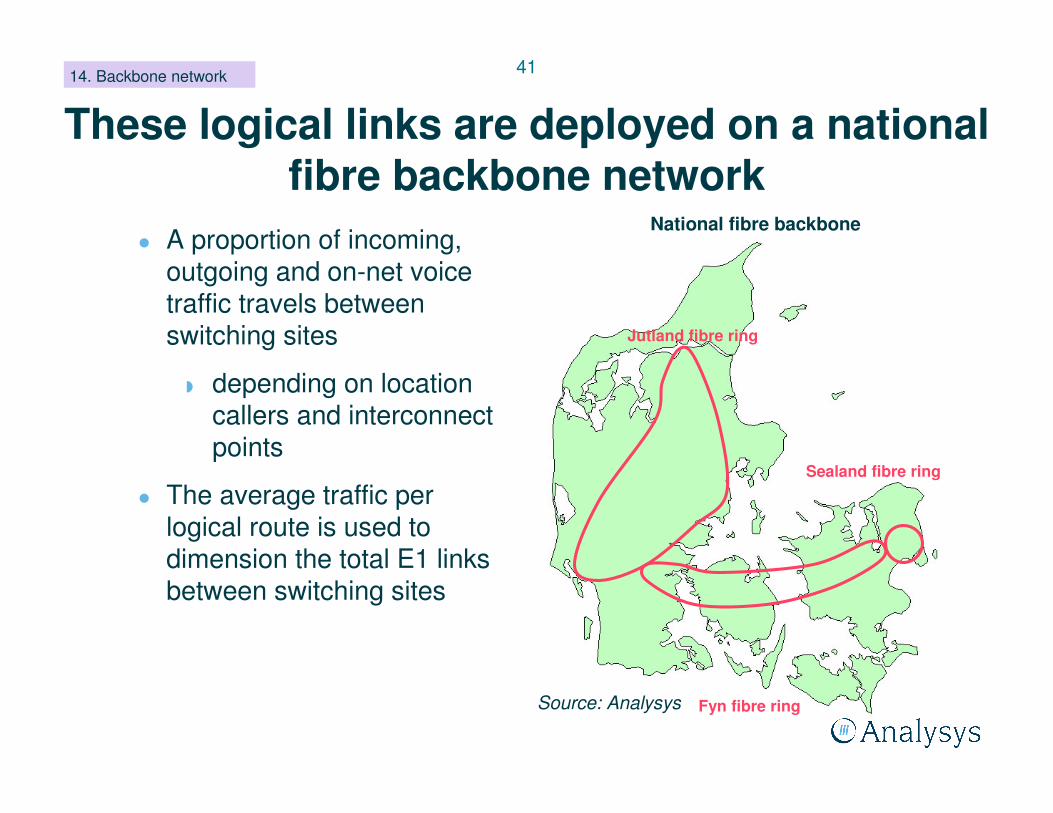
These logical links are deployed on a national fibre backbone network

� A proportion of incoming, outgoing and on-net voice traffic travels between switching sites

w depending on location callers and interconnect points

� The average traffic per logical route is used to dimension the total E1 links between switching sites


Fyn fibre ring

Fyn fibre ring

National fibre backbone

Jutland fibre ring

Fyn fibre ring

Sjaelland fibre ring

Jutland fibre ring

Fyn fibre ring

Sealand fibre ring

Source: Analysys

42

Backbone E1 links are distributed across the fibre rings

� We have estimated the proportion of transmission which occurs in the various parts of the country

� The total number of logical E1 links in each ring is calculated according to these proportions

� The number of E1 links per physical route is calculated

� Physical E1 links are then provisioned on STM-1 links (subject to max. utilisation), with length depending on the ring


400km600km50kmRing length

50%50%0%Backhaul access node links

34%33%33%Remote BSC–MSC links

25%25%50%Inter-switch E1s

JutlandFunenZeeland

Backbone E1 distribution

Source: Analysys

43

Data servers are deployed using straightforward rules

� Peak SMS throughput is calculated

� SMSC has a peak throughput capacity, subject to max. utilisation

� SGSN load in terms of simultaneously connected (2G+3G) subscribers is calculated

� GGSN load in terms of (2G+3G) active PDP contexts is calculated

� SGSNs and GGSNs have a defined capacity, subject to max. utilisation

15. SMSC, GSNs

SMSC SGSN and GGSN

44

Asset purchase is according to 1. deployment lead times, and 2. replacement lifetimes� Model calculates active

network assets at mid-year

� Capital expenditures on assets occurs 1–18 months in advance of activation

w depending on lead times and size of network assets

� Operating expenditures incurred once activated

� Replacement lifetime (5–25 years) determines when asset is replaced at current cost


Time

Demand requirement (t)subject to max.

utilisationLook-ahead

period

Ord

erin

gP

urch

asin

gD

eplo

ymen

tTe

stin

gA

ctiv

atio

n

Dep

loym

ent

Purchase requirement

subject to look-ahead

Lead time expenditure profile

Source: Analysys

45

Network elements are removed from the network when no longer required

� Due to migration off the networks, traffic-driven assets may become unnecessary, although coverage rules still apply

� The rate at which assets are removed from the network is an input to the model

� Removal saves:

w asset replacement costs

w operating expenditures

� Investment costs are still fully recovered; but removal is considered cost-less with zero scrap value


Time

Dep

loym

ent

Actual requirement according to

demand

t=1 t=2 t=100

Retirement options

Source: Analysys

46

The draft demand and network model contains indicative unit costs

� A schedule of capital and operating expenditures per network element is provided in the draft demand and network model

w along with annual price trends for these expenditures to drive the series of unit prices over time, and control the shape of the economic depreciation curve

� These unit cost inputs are indicative, based on previous LRIC models

� These unit costs allow the action of the purchasing and depreciation algorithms to be examined

17. Unit costs

47

The model contains a four-part mark-up , without any defined common costs (yet)

18. Incremental costs

Dedicated 2G assets

Incremental

Applicable to 2G-only services

Dedicated 2G assets –common

Dedicated 3G assets

Incremental

Applicable to 3G-only services

Dedicated 3G assets –common

Shared assets

Incremental

Applicable to 2G and 3G services

Shared assets – common

Retail incremental and common costs

Business overhead common costs

2G 3G

shared

overheads

Mark-up sequenceIncremental and common cost components

Source: Analysys

48

Agenda




Next steps

49

Agenda




Next steps

50

Next steps

� Operator progress on top-down data and/or models?

� NITA to distribute model and documents to mobile operators on Monday

� Analysys to receive top-down cost data in the coming week, top-down models in four weeks’ time

� Analysys to develop Tele2 version of this model

� Questions or clarifications on the model during the consultationperiod to NITA (cc Analysys if preferred)

� Possibility of next visit according to timetable

� Responses due 29 October 2007

51

Concluding remarks on the model – some calculations which could be improved� Dimensioning of 3G R99 packet data in radio

network: no effort, best efforts, or guaranteed effort?

� Tele2’s 3G traffic (carried as national roaming by Sonofon) does not have a ‘ON NR 3G service’ yet

� The cost allocation of the national backbone fibre network is not divided between all of backhaul, BSC-MSC and inter-switch services

w which could be done on an E1 basis

52

Contact details

� For NITA:

Michael Bøgh

3435 0261

[email protected]

� For Analysys:

Ian Streule

+44 1223 460600

[email protected]

Documents

NITA’s mobile LRAIC model - Erhvervsstyrelsen · NITA’s mobile LRAIC model ... HLR dimensioning w excluded from the traffic- ... w equivalent to 4 CE 6. Data demand drivers