Embed Size (px)
Citation preview

Nitinol FEA: Beyond ythe Fundamentals
Kenneth E. PerryP l E L b iPaul E. Labossiere
ECHOBIO LLC
OutlineOutline• Role of FEA in Design• Nitinol Material Model CalibrationNitinol Material Model Calibration• FEA Fundamentals• FEA Not so FundamentalsFEA Not so Fundamentals• Producing Valid Data• Verification of ResultsVerification of Results
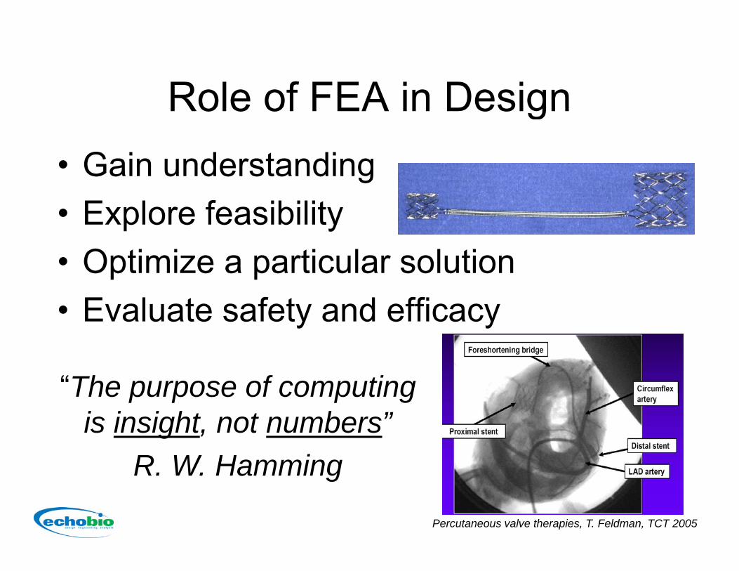
Role of FEA in DesignRole of FEA in Design• Gain understandingg• Explore feasibility
O ti i ti l l ti• Optimize a particular solution• Evaluate safety and efficacya ua e sa e y a d e cacy
“The purpose of computingThe purpose of computing is insight, not numbers”
R W Hamming
Percutaneous valve therapies, T. Feldman, TCT 2005
R. W. Hamming

Implants Break!Implants Break!
P. Chowdhury, R. Ramos, Coronary-Stent Fracture, New England Journal of Medicine, Volume 347:581,
McKelvey AL, Ritchie RO., J. Biomed. Mater. Res. 1999;47(3):301-308.
August 22, 2002, Number 8 (Commentary courtesy of B. Berg)
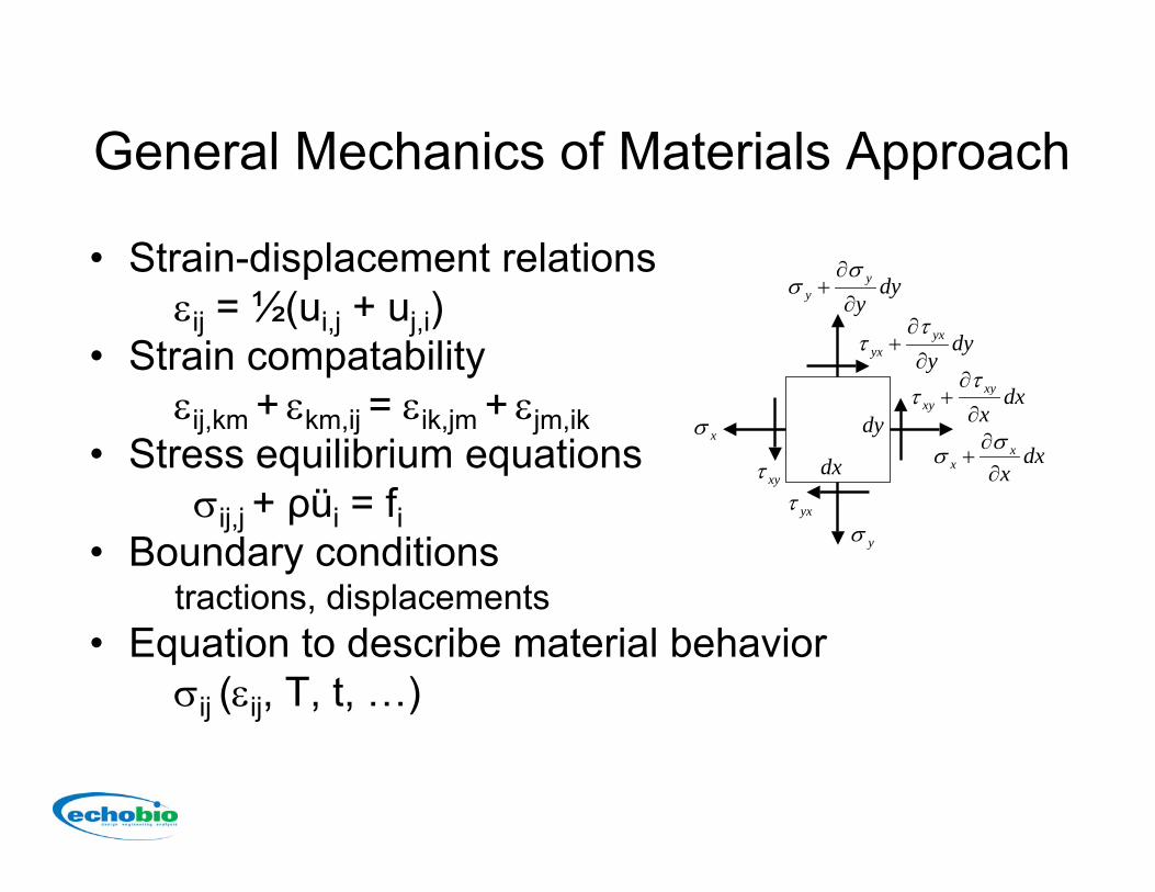
General Mechanics of Materials ApproachGeneral Mechanics of Materials Approach
• Strain-displacement relationsy∂σp
εij = ½(ui,j + uj,i)• Strain compatability
dyy
yy ∂+σ
dyyyx
yx ∂
∂+
ττ
dxy∂τεij,km + εkm,ij = εik,jm + εjm,ik
• Stress equilibrium equationsσ + ρü = f
dxx
xx ∂
∂+
σσxσ
dxxxy
xy ∂+τ
xyττ
dx
dy
σij,j + ρüi = fi• Boundary conditions
tractions, displacements
yσyxτ
p• Equation to describe material behavior
σij (εij, T, t, …)

Superelastic Behavior of NitinolSuperelastic Behavior of Nitinol– Stress induced reverse
transformation, T > Af
250
500
00 0.02 0.04 0.06
Shape Memory
750
p y– Thermally induced reverse
transformation, T < Af
250
500
00 0.02 0.04 0.06
HeatingNDC Website, www.nitinol.com

Generating Calibration Test DataGenerating Calibration Test Data• Measurements
– Load– Cross head disp.– Extensometer strain– TemperatureTemperature
• Complications– Multi-phase material
Loading mode dependence– Loading mode dependence– Temperature sensitivity– Large deformations
A i tK. Perry and P. Labossiere, ASTM 2005
– Anisotropy
“It is of no use to employ great sophisticationp y g pin computing outputs if your inputs are wrong”
Material Model ApproachesMaterial Model Approaches
• Piecewise continuous models• Piecewise continuous models• Hyperelasticity modelsHyperelasticity models• User Subroutines (UMATs)
–Generalized plasticity–Multi-phase elasticity
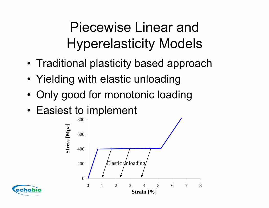
Piecewise Linear and H l i i M d lHyperelasticity Models
• Traditional plasticity based approachTraditional plasticity based approach• Yielding with elastic unloading
O l d f t i l di• Only good for monotonic loading• Easiest to implement
600
800
ss [M
pa]
200
400Stre
s
Elastic unloading
00 1 2 3 4 5 6 7 8
Strain [%]
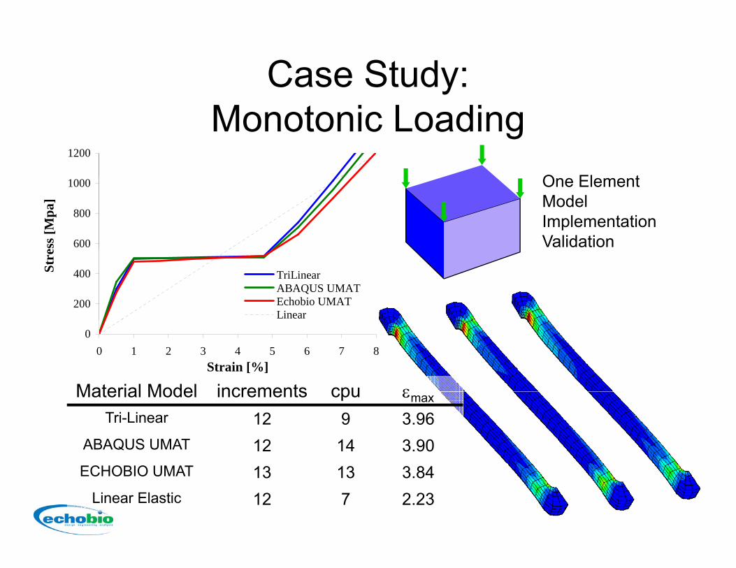
Case Study: M i L diMonotonic Loading
O El t
1200
One ElementModelImplementationValidation600
800
1000
ss [M
pa]
200
400Stre
TriLinearABAQUS UMATEchobio UMATLinear
Material Model increments cpu ε
00 1 2 3 4 5 6 7 8
Strain [%]
Material Model increments cpu εmax
Tri-Linear 12 9 3.96ABAQUS UMAT 12 14 3.90ECHOBIO UMAT 13 13 3.84
Linear Elastic 12 7 2.23
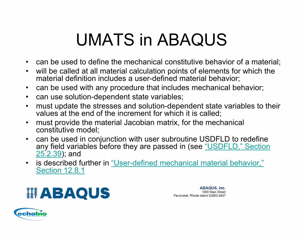
UMATS in ABAQUSUMATS in ABAQUS• can be used to define the mechanical constitutive behavior of a material;• will be called at all material calculation points of elements for which thewill be called at all material calculation points of elements for which the
material definition includes a user-defined material behavior;• can be used with any procedure that includes mechanical behavior;• can use solution-dependent state variables;• must update the stresses and solution-dependent state variables to their
values at the end of the increment for which it is called;• must provide the material Jacobian matrix, for the mechanical
constitutive model;constitutive model;• can be used in conjunction with user subroutine USDFLD to redefine
any field variables before they are passed in (see “USDFLD,” Section 25.2.39); andi d ib d f th i “U d fi d h i l t i l b h i ”• is described further in “User-defined mechanical material behavior,” Section 12.8.1
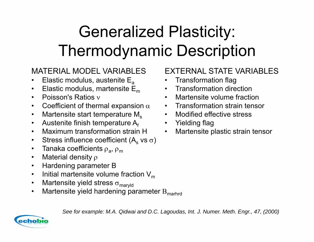
Generalized Plasticity: Th d i D i iThermodynamic Description
MATERIAL MODEL VARIABLES EXTERNAL STATE VARIABLES• Elastic modulus, austenite Ea• Elastic modulus, martensite Em• Poisson's Ratios ν• Coefficient of thermal expansion α
• Transformation flag• Transformation direction• Martensite volume fraction• Transformation strain tensor• Coefficient of thermal expansion α
• Martensite start temperature Ms• Austenite finish temperature Af• Maximum transformation strain H
• Transformation strain tensor• Modified effective stress• Yielding flag• Martensite plastic strain tensor
• Stress influence coefficient (As vs σ) • Tanaka coefficients ρa, ρm• Material density ρ• Hardening parameter BHardening parameter B• Initial martensite volume fraction Vm• Martensite yield stress σmaryld• Martensite yield hardening parameter Βmarhrd
See for example: M.A. Qidwai and D.C. Lagoudas, Int. J. Numer. Meth. Engr., 47, (2000)
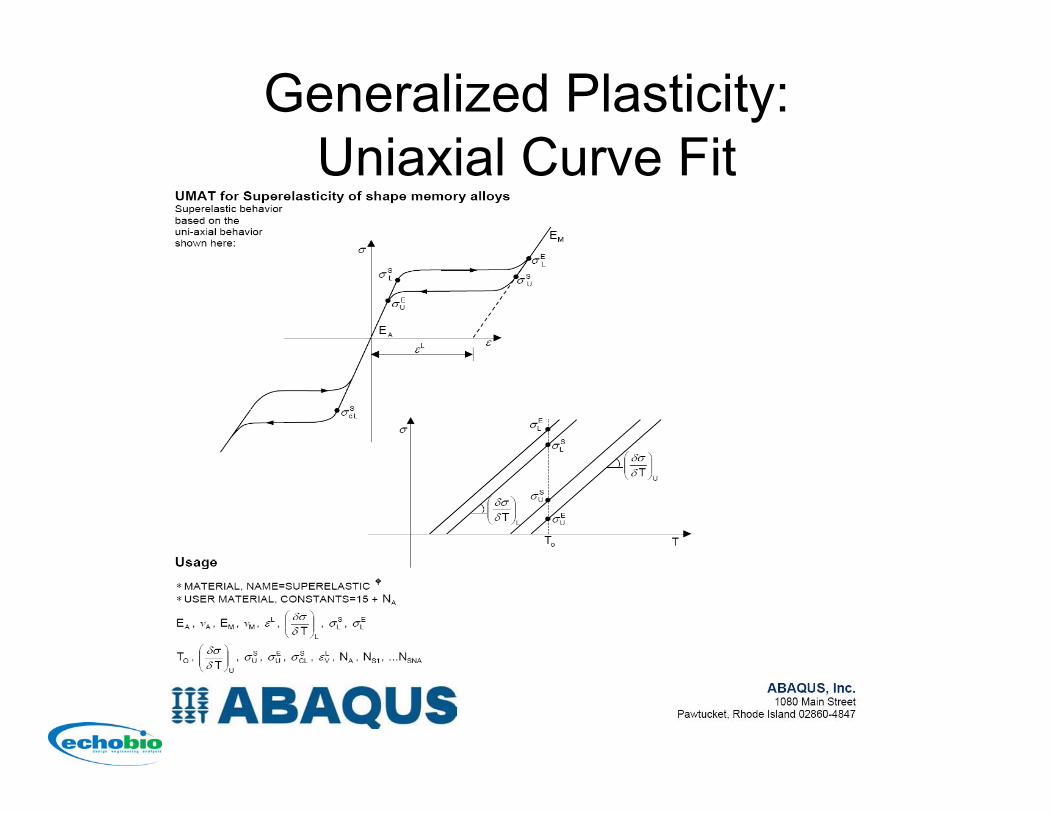
Generalized Plasticity:Uniaxial Curve FitUniaxial Curve Fit

Case Study:L di d U l diLoading and Unloading
0.5
0.3
0.4
e/St
rut
0.1
0.2Forc
e
TriLinearABAQUS UMATEchobio UMAT
Material Model cpu ε δ
00 1 2 3
Change in Radius [mm]
Linear
Material Model cpu εfinal δfinal
Tri-Linear 14 tons 1.14ABAQUS UMAT 42 0 0ECHOBIO UMAT 36 0 0
Linear Elastic 12 0 0

ConsiderationsConsiderations• 3D formulation?• Monotonic only loading?• Monotonic only loading?• Temperature dependence?• History dependence?
0.650 degrees
0 3
0.4
0.5
e/St
rut
50 deg ees37 degrees20 degrees0 degrees
ΔT0.1
0.2
0.3
Forc
e
00 1 2 3
Change in Radius [mm]
ΔT

Load History DependenceLoad History Dependence• Evolution of the stress-strain behavior after
multiple cycles of loadingmultiple cycles of loading
S. Miyazaki, Shape Memory Alloys, 1996Memory Alloys, 1996
0.4
0.5
Stru
t800
1000
1200
pa]
0 1
0.2
0.3
Rad
ial F
orce
/
First cycle
400
600
800
Stre
ss [M
p
First cycle
0
0.1
0 1 2 3Change in Radius [mm]
First cycleAfter 50 cycles
0
200
0 1 2 3 4 5 6 7 8Strain [%]
s cyc eAfter 50 cycles

Verification withE i l MExperimental Measurements
X-Y Gong, A.R. Pelton, T.W. Duerig, N. Rebelo and K.E. Perry, SMST 2003
400
500PP
δ
100
200
300
Load
, P [N
]
Path 1Path 2Path 3Path 4FEA solution
0
100
0 0.025 0.05 0.075 0.1 0.125 0.15 0.175 0.2
Displacement, δ [mm] -0.00 0.00 0.01 0.02 0.03 0.04-0.00 0.00 0.01 0.02 0.03 0.04K.E. Perry and P.E. Labossiere, SMST 2003
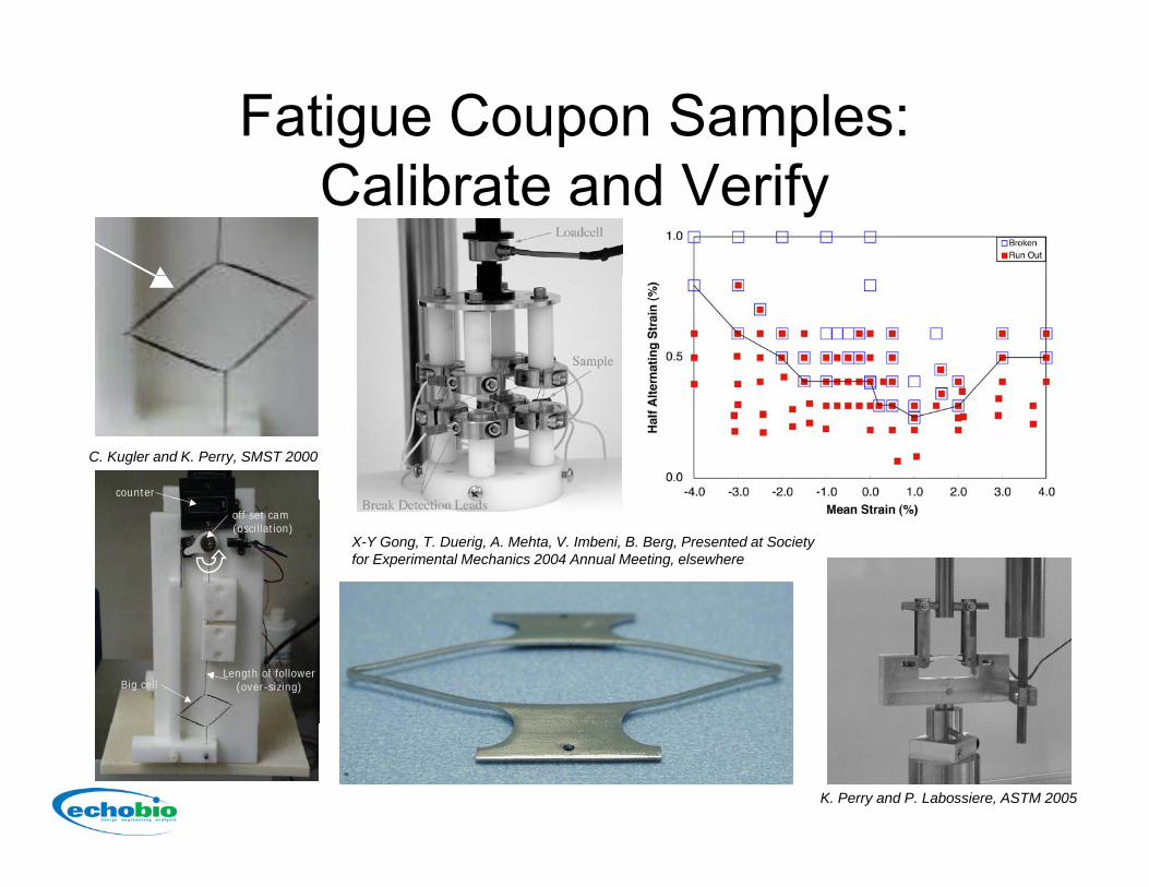
Fatigue Coupon Samples:C lib d V ifCalibrate and Verify
counter
C. Kugler and K. Perry, SMST 2000
off set cam (oscillation)
X-Y Gong, T. Duerig, A. Mehta, V. Imbeni, B. Berg, Presented at Society for Experimental Mechanics 2004 Annual Meeting, elsewhere
Big cellLength of follower
(over-sizing)
K. Perry and P. Labossiere, ASTM 2005
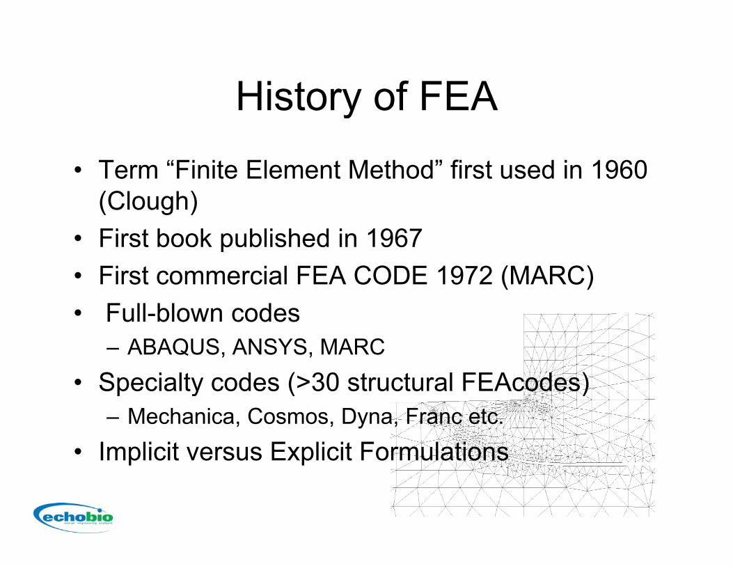
History of FEAHistory of FEA
• Term “Finite Element Method” first used in 1960Term Finite Element Method first used in 1960 (Clough)
• First book published in 1967p• First commercial FEA CODE 1972 (MARC)• Full-blown codesFull blown codes
– ABAQUS, ANSYS, MARC• Specialty codes (>30 structural FEAcodes)Specialty codes ( 30 structural FEAcodes)
– Mechanica, Cosmos, Dyna, Franc etc.• Implicit versus Explicit Formulationsp p
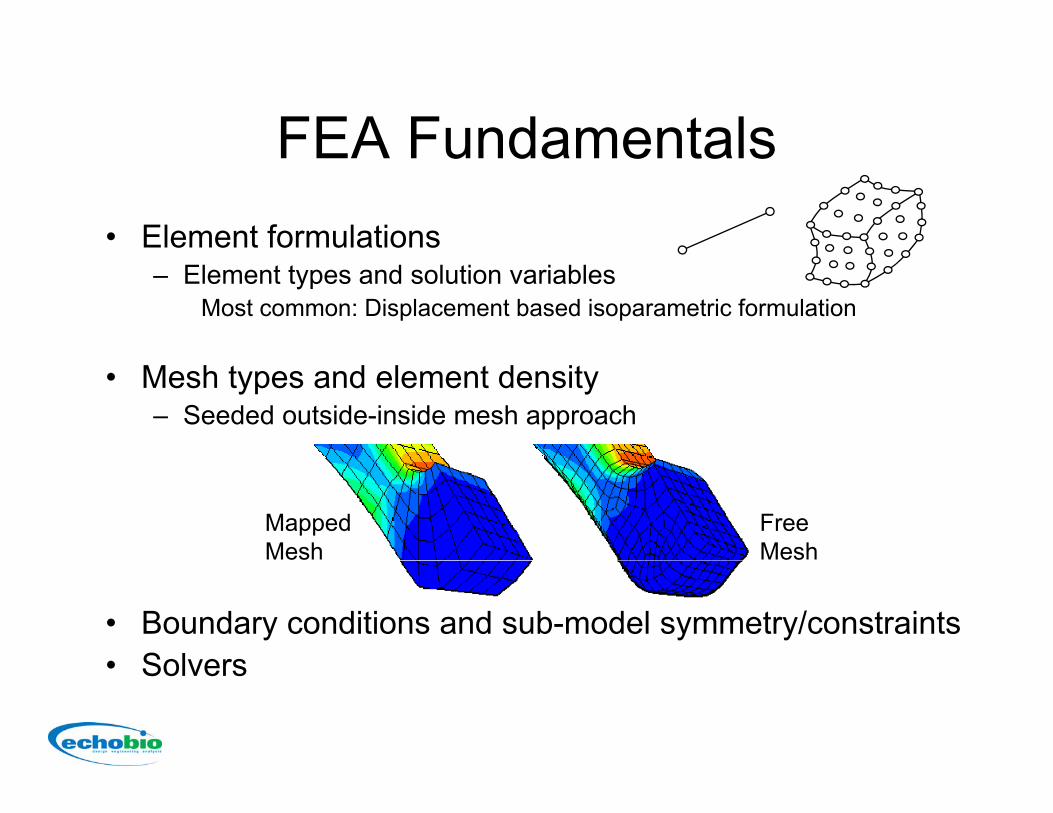
FEA FundamentalsFEA Fundamentals• Element formulations
– Element types and solution variablesMost common: Displacement based isoparametric formulation
• Mesh types and element density– Seeded outside-inside mesh approach
MappedMesh
FreeMesh
• Boundary conditions and sub-model symmetry/constraints• Solvers• Solvers

Element FormulationsElement Formulations• Linear Elements-2 nodes per edgep g
– Linear geometrical and displacement description
– Constant (triangles) or ( g )quasi-linear (squares) stress and strain description
• Quadratic Elements-3 nodes per edge– Quadratic geometrical and
displacement description5
3
5
3
displacement description– Linear (triangles) or
quasi-quadratic (squares)stress and strain description
1
4
6 2
1
4
6 2
stress and strain description

Elements in BendingElements in Bending• Some elements do not perform well in bending because
that deformation is not well described by the elementthat deformation is not well described by the element formulation– Linear isoparametric elements
• Element that do better in bending– Higher order elements (quadratic elements and up)– Reduced integration elements educed teg at o e e e ts– Bending specific elements such as incompatible mode elements
• ExampleElement Type # of DOF Max Deflectionyp
CST 24 0.3LST 30 0.99
Lin. Brick 24 .69Q d B i k 26 1 03Quad. Brick 26 1.03
Modified Bilinear 36 1.02Analytical - 1.0

FEA Basic PrincipleFEA Basic Principle
The static FEA solution (for displacementThe static FEA solution (for displacement formulation) comes from:
0=∫∫∫ ∫∫∫∫∫ TTT dSdVdV TNXNPuDBB
or simply
0=−−− ∫∫∫ ∫∫∫∫∫V S
tractbodyV
dSdVdV TNXNPuDBB
0=− fuKor simplyand with inertial and viscous effects
fKuuCuM =++ &&&
0=− fuK
With geometric and material nonlinearities, the problem becomes much more complicated
fKuuCuM ++

ComplicationsComplications• Nonlinear Material (ex: plasticity)
)(1 DnmDmDnH
DD ⋅⊗⋅⋅⋅+
−= &&&&p
ep
• Large deformationsp
( )∫∫∫ ++=v
OTLL
TLL
TOL dVDBBDBBDBBK
• Finite strains
⎥⎤
⎢⎡
⎟⎞
⎜⎛ ∂+⎟
⎞⎜⎛ ∂+⎟
⎞⎜⎛ ∂+
∂ 2221 wvuuε⎥⎥⎦⎢
⎢⎣
⎟⎠
⎜⎝ ∂
+⎟⎠
⎜⎝ ∂
+⎟⎠
⎜⎝ ∂
+∂
=2 xxxxxε
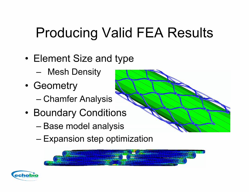
Producing Valid FEA ResultsProducing Valid FEA Results
• Element Size and typeElement Size and type– Mesh Density
Geometry• Geometry– Chamfer Analysis
• Boundary Conditions– Base model analysis– Expansion step optimization
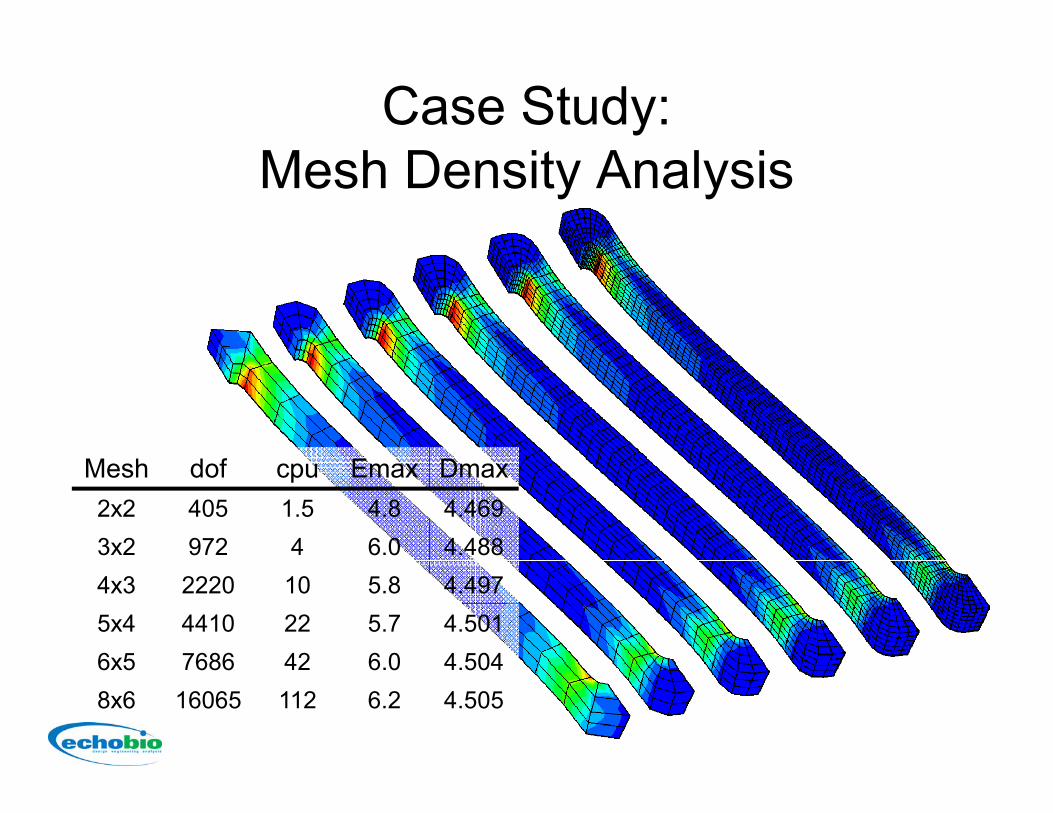
Case Study:M h D i A l iMesh Density Analysis
Mesh dof cpu Emax Dmax2x2 405 1.5 4.8 4.4693x2 972 4 6.0 4.4884x3 2220 10 5.8 4.4975x4 4410 22 5.7 4.5016x5 7686 42 6 0 4 5046x5 7686 42 6.0 4.5048x6 16065 112 6.2 4.505

Case Study:Ch f A l iChamfer Analysis
Displacementpbased BC’s
Model EmaxRectangular 5 59Rectangular 5.59
50µm Chamfer 5.99
100µm chamfer 5.84
Fillet Radius = 100µm 5.68
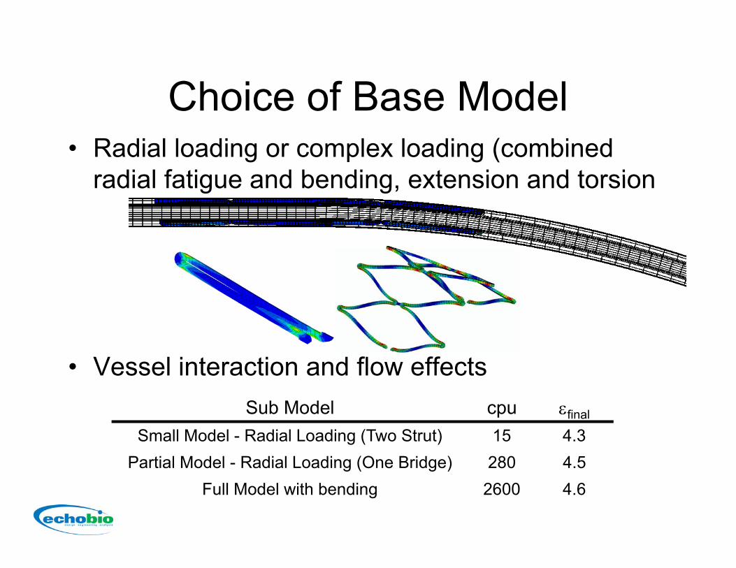
Choice of Base ModelChoice of Base Model• Radial loading or complex loading (combined
radial fatigue and bending extension and torsionradial fatigue and bending, extension and torsion
• Vessel interaction and flow effectsSub Model cpu εfinal
Small Model - Radial Loading (Two Strut) 15 4.3Partial Model - Radial Loading (One Bridge) 280 4 5Partial Model - Radial Loading (One Bridge) 280 4.5
Full Model with bending 2600 4.6
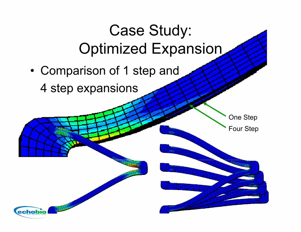
Case Study:O i i d E iOptimized Expansion
• Comparison of 1 step andComparison of 1 step and 4 step expansions
One Step
Four StepFour Step
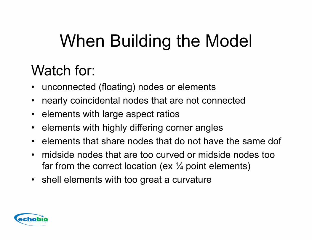
When Building the ModelWhen Building the ModelWatch for:Watch for:• unconnected (floating) nodes or elements• nearly coincidental nodes that are not connectedy• elements with large aspect ratios• elements with highly differing corner angles• elements that share nodes that do not have the same dof• midside nodes that are too curved or midside nodes too
far from the correct location (ex ¼ point elements)far from the correct location (ex ¼ point elements)• shell elements with too great a curvature
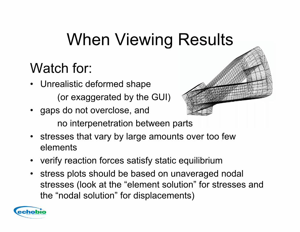
When Viewing ResultsWhen Viewing ResultsWatch for:Watch for:• Unrealistic deformed shape
(or exaggerated by the GUI)( gg y )• gaps do not overclose, and
no interpenetration between parts• stresses that vary by large amounts over too few
elements• verify reaction forces satisfy static equilibrium• verify reaction forces satisfy static equilibrium• stress plots should be based on unaveraged nodal
stresses (look at the “element solution” for stresses and (the “nodal solution” for displacements)
FEA Not So FundamentalsFEA Not So Fundamentals• Convergenceg
– Solution Stabilization• Nonlinearities
– Material– Geometry (large deformation/finite strain)
Boundary Conditions and Interactions• Boundary Conditions and Interactions– Contact surfaces
• User Subroutines and working with FEA codesUser Subroutines and working with FEA codes outside of the box– UMATS and feedback loops
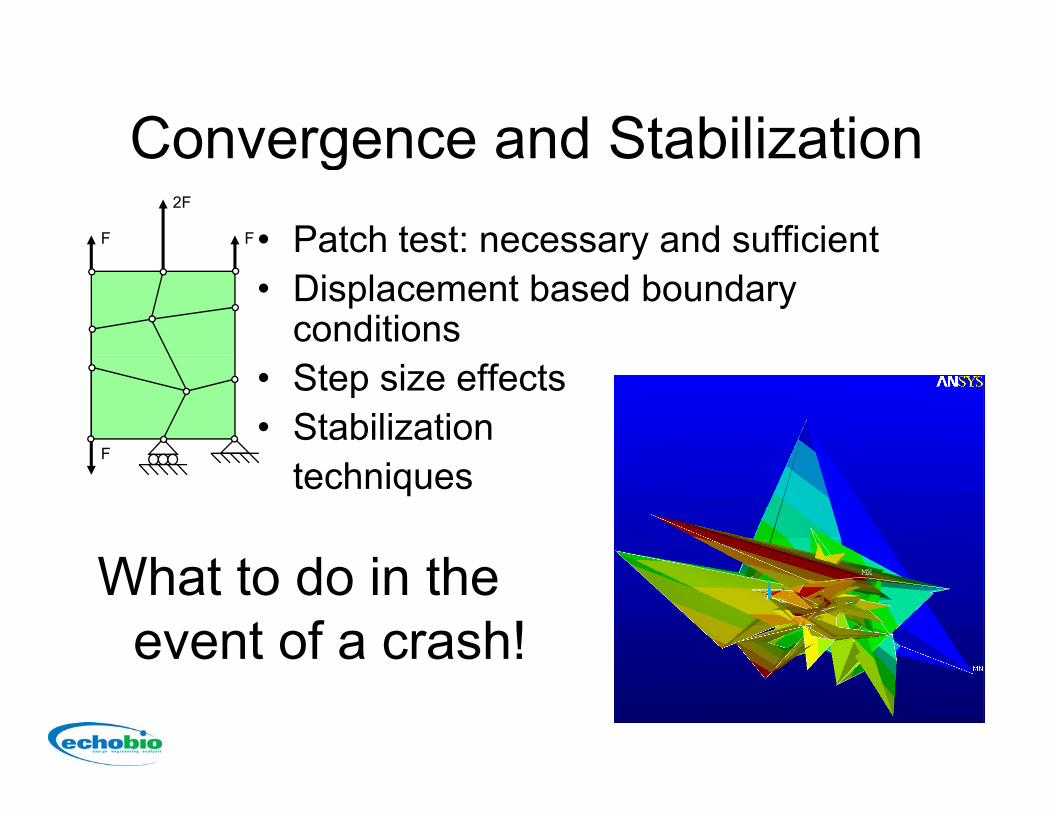
Convergence and Stabilization• Patch test: necessary and sufficient
Convergence and StabilizationF
2F
F y• Displacement based boundary
conditions• Step size effects• Stabilization
F
techniquesF
Wh t t d i thWhat to do in theevent of a crash!
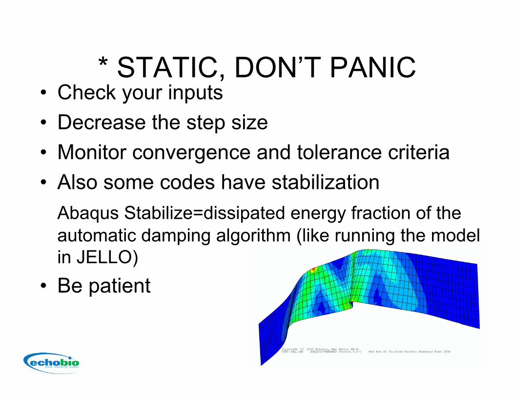
* STATIC DON’T PANIC STATIC, DON T PANIC• Check your inputs• Decrease the step size• Decrease the step size• Monitor convergence and tolerance criteria• Also some codes have stabilization
Abaqus Stabilize=dissipated energy fraction of the automatic damping algorithm (like running the model in JELLO)
• Be patient
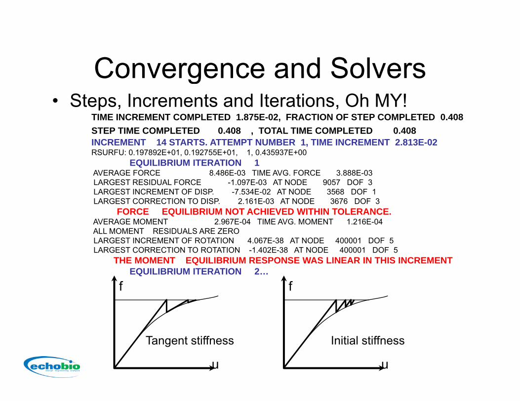
Convergence and SolversConvergence and Solvers• Steps, Increments and Iterations, Oh MY!
TIME INCREMENT COMPLETED 1.875E-02, FRACTION OF STEP COMPLETED 0.408 STEP TIME COMPLETED 0.408 , TOTAL TIME COMPLETED 0.408INCREMENT 14 STARTS. ATTEMPT NUMBER 1, TIME INCREMENT 2.813E-02RSURFU: 0.197892E+01, 0.192755E+01, 1, 0.435937E+00
EQUILIBRIUM ITERATION 1AVERAGE FORCE 8.486E-03 TIME AVG. FORCE 3.888E-03AVERAGE FORCE 8.486E 03 TIME AVG. FORCE 3.888E 03LARGEST RESIDUAL FORCE -1.097E-03 AT NODE 9057 DOF 3LARGEST INCREMENT OF DISP. -7.534E-02 AT NODE 3568 DOF 1LARGEST CORRECTION TO DISP. 2.161E-03 AT NODE 3676 DOF 3
FORCE EQUILIBRIUM NOT ACHIEVED WITHIN TOLERANCE.AVERAGE MOMENT 2.967E-04 TIME AVG. MOMENT 1.216E-04ALL MOMENT RESIDUALS ARE ZEROLARGEST INCREMENT OF ROTATION 4.067E-38 AT NODE 400001 DOF 5LARGEST CORRECTION TO ROTATION -1.402E-38 AT NODE 400001 DOF 5
THE MOMENT EQUILIBRIUM RESPONSE WAS LINEAR IN THIS INCREMENTEQUILIBRIUM ITERATION 2…
f f
u u
Tangent stiffness Initial stiffness

Case Study:Model Instabilities versusModel Instabilities versus
Solution Instabilitiese
[N]
STABLE REGION
05 10 15 20 25 30
Diameter [mm]ater
al F
orce
Diameter [mm]
La
UNSTABLE REGION
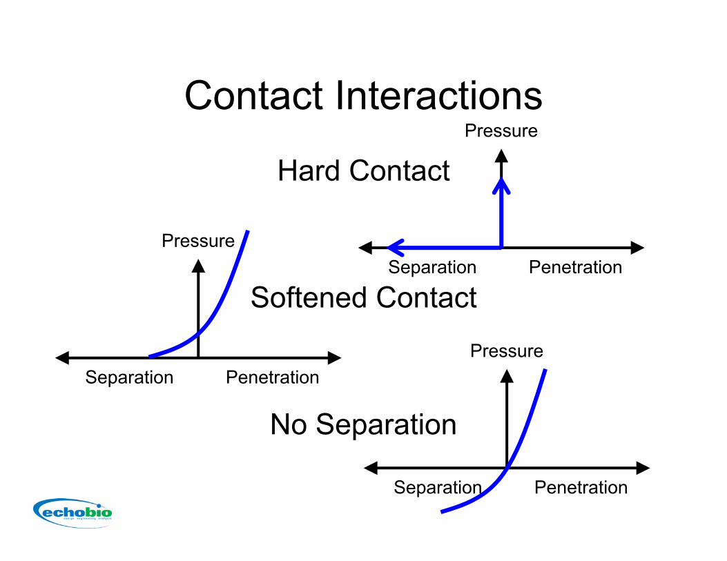
Contact InteractionsContact Interactions
Hard ContactPressure
Hard Contact
Pressure
Softened Contact
PressureSeparation Penetration
Separation PenetrationPressure
No Separation
p
Separation Penetration

Contact InteractionsContact Interactions
• Deformable contact bodiesDeformable contact bodies– Element based surfaces– Node based surfaces
• Rigid surface definitions• Self Contact
– to be included manually?
Element set
Node set

Radial Expansion, Crimp and F i M d liFatigue Modeling
• Radial loading with contracting and g gexpanding analytically defined cylinders
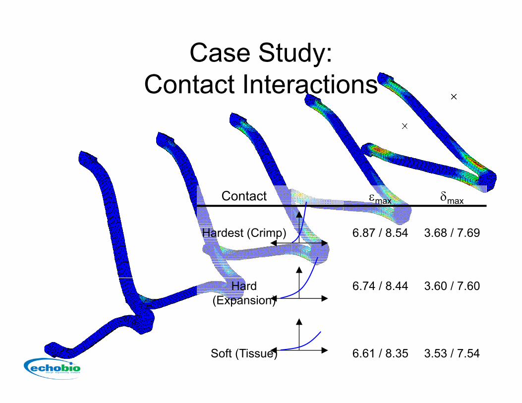
Case Study:C I iContact Interactions
Contact εmax δmax
Hardest (Crimp) 6.87 / 8.54 3.68 / 7.69
Hard (Expansion)
6.74 / 8.44 3.60 / 7.60
Soft (Tissue) 6.61 / 8.35 3.53 / 7.54
Verification of Results
• Perhaps a wordy slide to help accentuate
Verification of Results
Perhaps a wordy slide to help accentuate the importance of verification…and a list of possible ways verification can be donepossible ways verification can be done…
Di i l ifi ti– Dimensional verification (displacements are consistent)
– Radial force verification (equilibrium is satisfied)
F il / li bili l i– Failure/reliability analysis (material characterization is correct, self consistency)
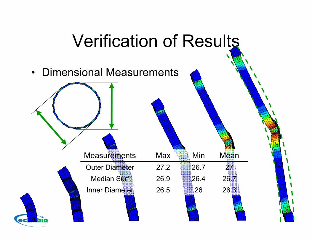
Verification of ResultsVerification of Results
• Dimensional MeasurementsDimensional Measurements
Measurements Max Min MeanOuter Diameter 27 2 26 7 27Outer Diameter 27.2 26.7 27
Median Surf 26.9 26.4 26.7Inner Diameter 26.5 26 26.3
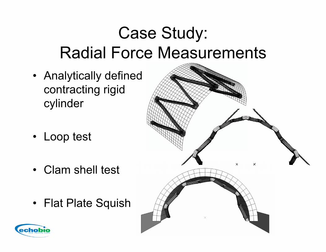
Case Study:R di l F MRadial Force Measurements
• Analytically definedAnalytically defined contracting rigid cylinder
• Loop testp
• Clam shell testC a s e test
• Flat Plate SquishFlat Plate Squish
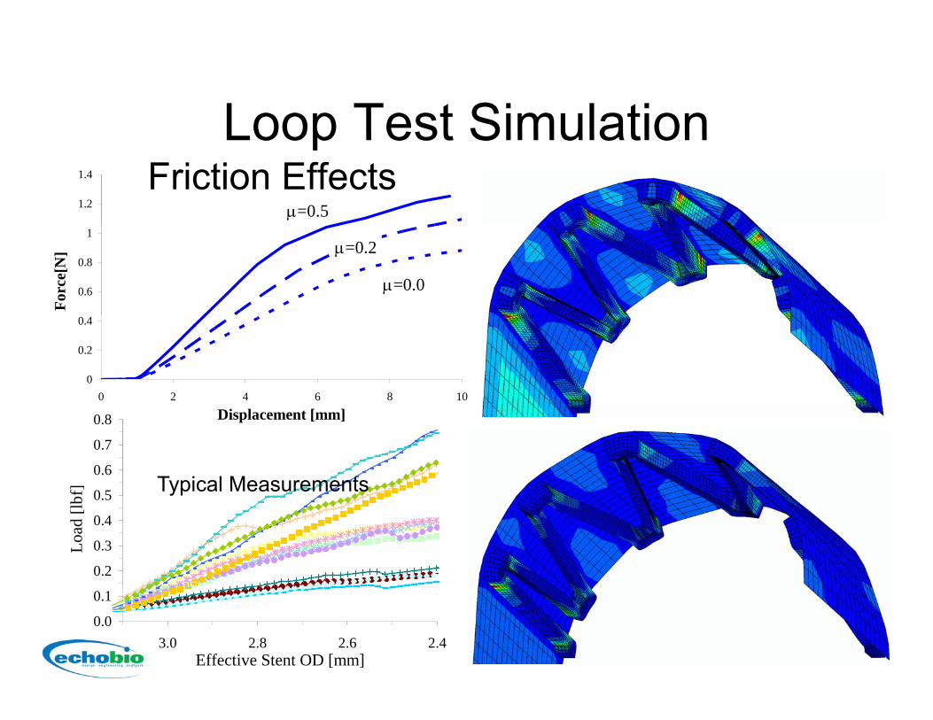
Loop Test SimulationLoop Test SimulationFriction Effects
1.2
1.4
μ=0.5
0.6
0.8
1
Forc
e[N
]
μ=0.0
μ=0.2
0
0.2
0.4
0 2 4 6 8 10
Displacement [mm]
0 5
0.6
0.7
0.8
f] Typical Measurements
0.2
0.3
0.4
0.5
Load
[lb
0.0
0.1
2.42.62.83.0Effective Stent OD [mm]
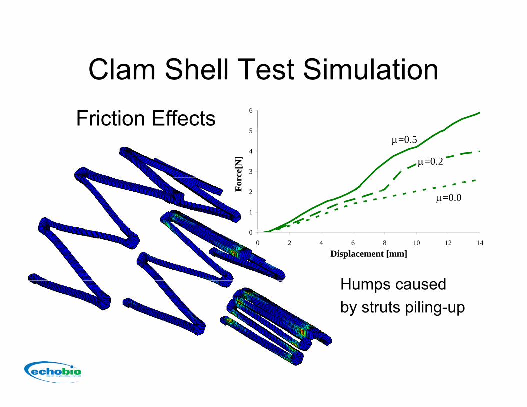
Clam Shell Test SimulationClam Shell Test Simulation6Friction Effects
3
4
5
rce[
N]
μ=0.5
μ=0.2
1
2For
μ=0.0
00 2 4 6 8 10 12 14
Displacement [mm]
H dHumps causedby struts piling-up

Fatigue and ReliabilityFatigue and Reliability• For medical devices, success comes down
to reliability with failure due to fatigue• In-vitro Fatigue testingIn vitro Fatigue testing
– Test-to-success versus Test-to-failure• In vitro fatigue model verification• In-vitro fatigue model verification• Results interpretation
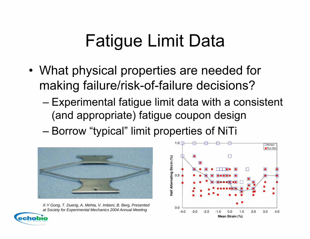
Fatigue Limit DataFatigue Limit Data• What physical properties are needed forWhat physical properties are needed for
making failure/risk-of-failure decisions? – Experimental fatigue limit data with a consistentExperimental fatigue limit data with a consistent
(and appropriate) fatigue coupon design– Borrow “typical” limit properties of NiTio o typ ca t p ope t es o
X-Y Gong, T. Duerig, A. Mehta, V. Imbeni, B. Berg, Presented at Society for Experimental Mechanics 2004 Annual Meeting
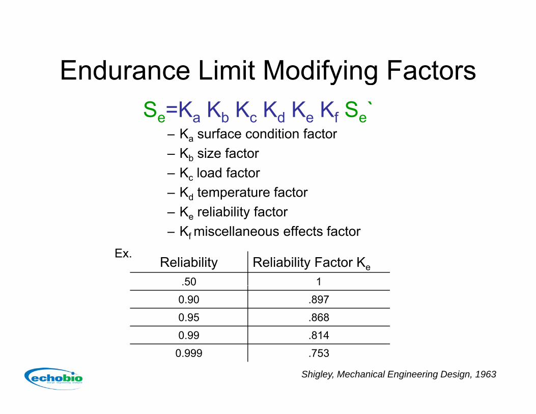
Endurance Limit Modifying FactorsEndurance Limit Modifying FactorsSe=Ka Kb Kc Kd Ke Kf Se`
K f di i f– Ka surface condition factor– Kb size factor– Kc load factor– Kd temperature factor– Ke reliability factor– Kf miscellaneous effects factorKf miscellaneous effects factor
Reliability Reliability Factor Ke
.50 1
Ex.
500.90 .8970.95 .8680 99 814
Shigley, Mechanical Engineering Design, 1963
0.99 .8140.999 .753
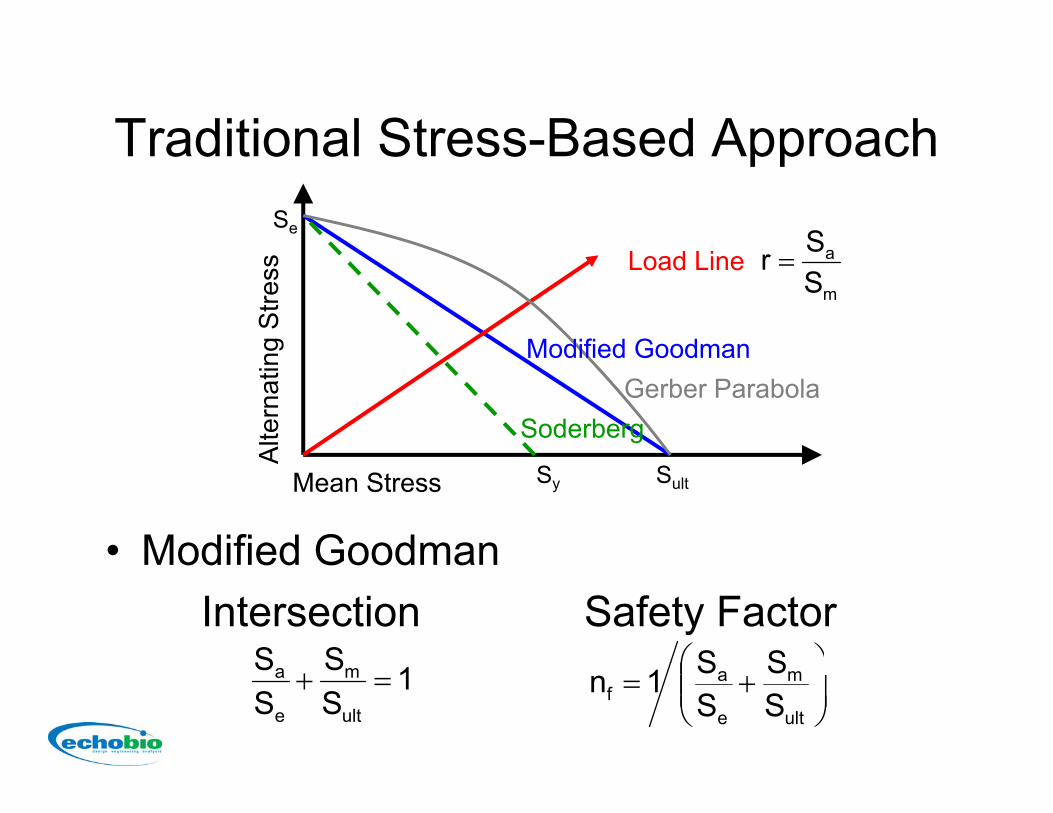
Traditional Stress-Based ApproachTraditional Stress Based ApproachSe
L d Li aSng
Stre
ss Load Line
Modified Goodman
m
a
Sr =
Alte
rnat
in
Gerber ParabolaModified Goodman
Soderberg
• Modified Goodman
A
Sy SultMean Stress
Modified GoodmanIntersection Safety Factor
SS⎟⎞
⎜⎛ SS1
SS
SS
ult
m
e
a =+ ⎟⎟⎠
⎞⎜⎜⎝
⎛+=
ult
m
e
af S
SSS1n
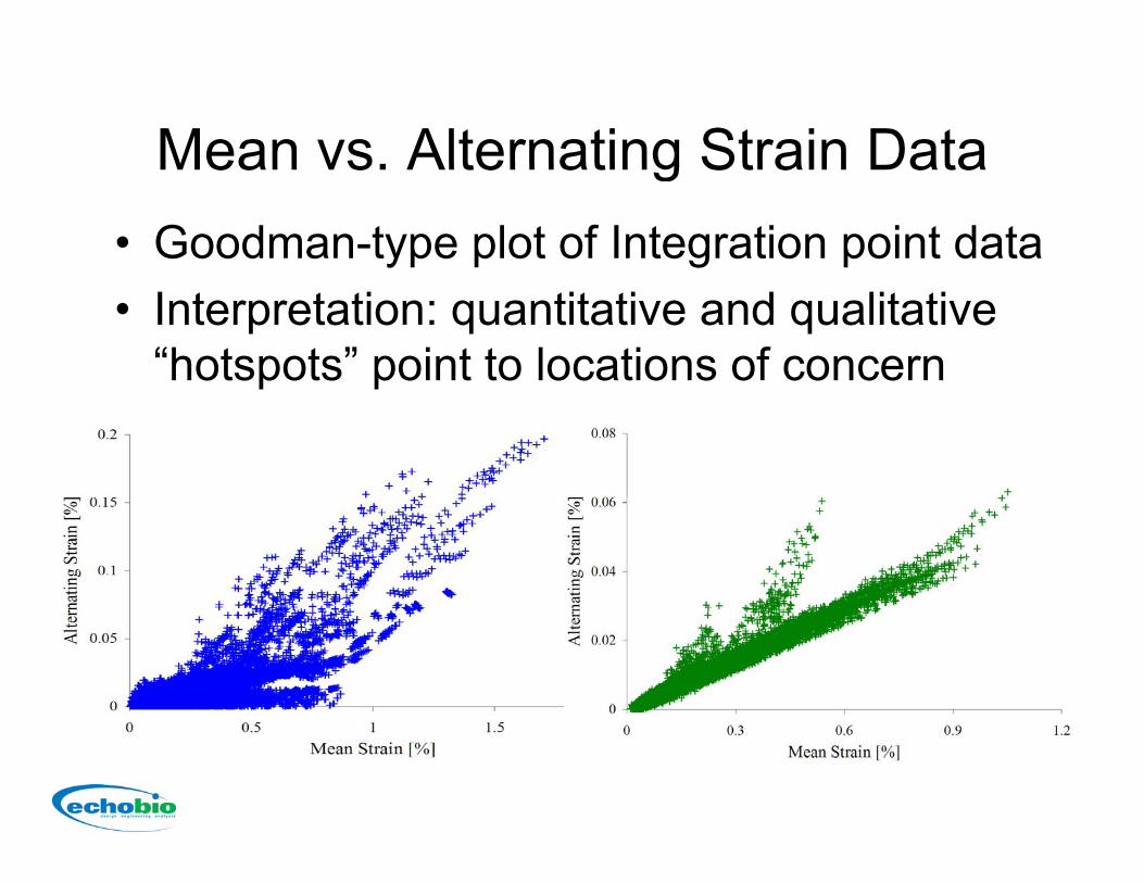
Mean vs Alternating Strain DataMean vs. Alternating Strain Data• Goodman-type plot of Integration point data• Interpretation: quantitative and qualitative
“hotspots” point to locations of concernp p
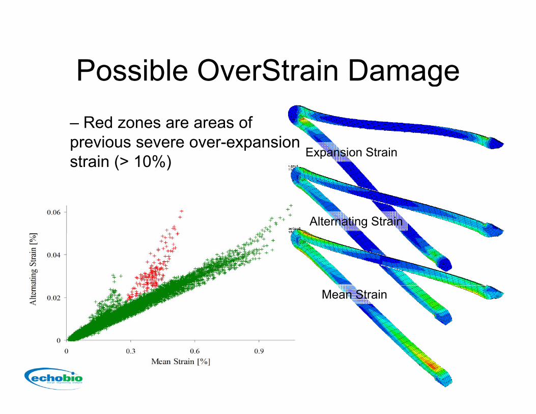
Possible OverStrain DamagePossible OverStrain Damage– Red zones are areas of
Expansion Strainprevious severe over-expansion strain (> 10%)
Alternating Strain
Mean Strain
Summary of Good FEA PracticesSummary of Good FEA Practices
Calibrate your modelValidate your methodology
and Verify your results