Embed Size (px)
Citation preview

NKS-449 ISBN 978-87-7893-541-0
EcoFood - A tool for assessment of
radiation exposure in terrestrialenvironments impacted by
airborne releases
Hosseini, A.1
Avila, R.2
Hryhorenko, D.2
Brown, J.1
Peltonen, T.3
Virtanen, S.3
Nielsen, S.4
Gudnason, K.5
1DSA (Norway) 2AFRY (Sweden)
3STUK(Finland) 4DTU(Denmark) 5IRSA (Iceland)
January 2021

Abstract The software package FDMT - Food Chain and Dose Module for Terres-trial Pathways is a component of the decision support systems, JRODOS and ARGOS, that are currently used in the Nordic countries for response to nuclear emergencies. Not all food chains that are relevant for the Nordic conditions are currently supported by FDMT and the modelling of some of the food chains is not optimal for the Nordic conditions, resulting in difficul-ties with the parameterization of the models. Moreover, in its current im-plementation FDMT is not totally transparent to users. The focus of the project was to develop a new software (EcoFood) that addresses these deficiencies and considers the findings of a gap analysis of FDMT con-ducted early in the project. The report presents the findings of the gap analysis, provides an overview of EcoFood´s components: the Simulator, the Model Library and the Parameter Database and a discussion on im-provements and advantages inherent to EcoFood. Key words radionuclide, releases, atmospheric, environment, terrestrial, dose, humans
NKS-449 ISBN 978-87-7893-541-0 Electronic report, June 2021 NKS Secretariat P.O. Box 49 DK - 4000 Roskilde, Denmark Phone +45 4677 4041 www.nks.org e-mail [email protected]

1
EcoFood - A tool for assessment of radiation exposure in
terrestrial environments impacted by airborne releases
Final Report from the NKS-B EcoFood (Contract: AFT/B(20)5)
Hosseini, Ali1
Avila, Rodolfo2
Hryhorenko, Dmytro2,
Koliabina, Daria2
Brown, Justin1,
Peltonen, Tuomas3
Virtanen, Sinikka3
Nielsen, Sven4
Gudnason, Kjartan5
1DSA, Norway 2AFRY, Sweden
3STUK, Finland
4DTU, Denmark
5IRSA, Iceland

2
Table of contents
1. Introduction.................................................................................................................................... 3
2. Gap analysis of FDMT ...................................................................................................................... 4
2.1. Soil models ................................................................................................................................... 4
2.2. Models for plants ........................................................................................................................ 5
2.3. Models for animals ..................................................................................................................... 6
2.5. Food chain parameters ............................................................................................................... 8
2.6. Uncertainty analysis .................................................................................................................11
2.7. Summary of the gap analysis ...................................................................................................12
3. Overview of EcoFood ......................................................................................................................13
3.1. The EcoFood Simulator ...........................................................................................................14
3.2. The EcoFood Model Library ...................................................................................................15
3.3. The EcoFood Parameter Database ..........................................................................................20
4. Improvements implemented in EcoFood .......................................................................................21
4.1. Models for soils .........................................................................................................................21
Intelligent distribution coefficients (Kds) ..................................................................................21
4.2. Models for plants ......................................................................................................................23
Intelligent Transfer Factors (TFs) .............................................................................................23
4.3. Models for animals ...................................................................................................................23
4.4. Uncertainty and sensitivity analyses ...........................................................................................24
Uncertainty analysis ....................................................................................................................24
Sensitivity analysis .......................................................................................................................25
5. Conclusions and recommendations ................................................................................................27
6. References .........................................................................................................................................29
Appendix. Conceptual and Mathematical Models ...........................................................................32

3
1. Introduction
The software package FDMT -Food Chain and Dose Module for Terrestrial Pathways (Müller
et al. 2004) is a component of the decision support systems, JRODOS and ARGOS, that are
currently used in the Nordic countries for response to nuclear emergencies. FDMT allows
modelling the transfer of radionuclides in terrestrial food chains following an atmospheric
deposition, to obtain estimates of radionuclide concentrations in foodstuffs and doses to the
public from their ingestion. Not all food chains that are relevant for the Nordic conditions are
currently supported by FDMT and the modelling of some of the food chains included in
JRODOS is not optimal for the Nordic conditions, resulting in difficulties with the
parameterization of the models. Moreover, in its current implementation FDMT is not totally
transparent to users.
This report presents the results of the NKS funded project EcoFood, implemented during 2020-
2021. The focus of the project was to develop a new software (EcoFood) that addresses the
above-mentioned deficiencies of FDMT and considering the findings of a gap analysis of
FDMT conducted early in the project. The final goal of the project was to achieve a tool suitable
for the Nordic conditions and that can be used in standalone mode, i.e., outside ARGOS and
JRODOS.
The report consists of six main Sections. Section 2 presents the findings and conclusions of the
gap analysis. Section 3 presents an overview of EcoFood. This Section is complemented by an
Appendix describing the conceptual and mathematical models included in EcoFood. Section
4 presents a discussion on improvements in EcoFood, as compared to FDMT. Conclusions
and recommendations for further development of EcoFood are provided in Section 5 and
references are listed in Section 6.

4
2. Gap analysis of FDMT
The project started with a gap analysis of FDMT. For this, the project team studied relevant
accident scenarios for FDMT application in the Nordic conditions and identified food chains
that need to be included in the modelling. The team then compared the food chains included
in FDMT and the modelling approaches with the identified needs for the Nordic countries. The
team also considered findings from international projects that have examined FDMT,
including:
PardNord and EcoDoses - NKS projects - these projects addressed improvements of
radioecological assessment of doses to man from terrestrial ecosystems and recommended
parameter values for Nordic conditions (Nielsen and Andersson, 2006, Nielsen and Andersson,
2008).
CONFIDENCE - EC project – The project addressed the issue of uncertainties in radiological
impact assessments. Also, some sub-models of FDMT were implemented in Ecolego (Brown
et al. 2018, Raskob et al. 2018).
COMET – EC project - has included efforts for improving human food chain modelling
through regional customization of parameter values, using Bayesian methods, and studying the
long‐term dynamics of soil‐to‐plant transfers for specific soil types and for long‐lived
radionuclides (Thorring et al. 2016).
The sub-sections 2.1-2.6 below present the findings in the different focus areas of the gap
analysis, and sub-section 2.7 presents a summary of features and functionalities that EcoFood
is expected to have.
2.1. Soil models
In the current version of FDMT, the radionuclide activity concentration available for root
uptake is modelled by accounting for post-depositional processes occurring in soil, these being
migration/leaching of the radionuclide out of the rooting zone and fixation in soil and
subsequent desorption. The soil model is formalised as the analytical solution to a system
comprising of two compartments, representing the activity available and not available (fixed)
for plants, with transfers (as rate constants representing the three processes above) between and
from the compartments (Müller et al., 2004). As default values, the desorption rate is set to
zero in FDMT and fixation rates of 2.2x10⁻⁴ d-1 for Cs and 9x10⁻⁵ d-1 for Sr are assumed (the
provenance of these values, within Müller et al. (2004), is however unclear). For other elements
it is assumed that fixation is of minor importance and is set to zero. Activity concentrations in
crops are derived via the multiplication of a transfer factor (commonly referred to as soil-plant
concentration ratios, in units of Bq/kg (f.w. plant) per Bq/kg (d.w. soil)) by the concentration
of activity (Bq kg-1) in the root zone of soil at time ‘t’ (Müller et al., 2004). The activity
concentration of a given radionuclide in the root zone is synonymous with the radionuclide
activity concentration available for root uptake as noted above.
It is possible to consider different soil types in a simplistic way in FDMT by altering various
parameters, notably migration/leaching rate, fixation, and desorption rates, for the soil -

5
processes module and by modifying the soil to crop transfer factor accordingly to make them
congruent with the specific soils the assessor is dealing with. If such changes are required, a
collation of empirical data specific to some of these parameters for given soil types is available
from publications such as IAEA (2010). However, limitations are apparent in relation to how
radionuclide behaviour in soils and transfer to plant/crop is modelled within FDMT, using the
empirical approach.
Long-term Assessment and hot Particles
Following severe nuclear events, a major fraction of refractory radionuclides will be released
as radioactive particles, containing fission and activation products such as 90Sr and 137Cs as
well as transuranic radionuclides. Knowledge with respect to particle characteristics and
processes influencing particle weathering in soils, i.e., the transformation of solid-state
radionuclide species bound in a particle matrix to dissolved species is a prerequisite for robust
prognoses. Essentially, information on potentially bioavailable forms (Kashparov et al., 2004)
is needed to assess long-term impact from radioactive particle contamination. The current
model in FDMT involving the behaviour of radionuclides in soils is, however, not suited to
modification. For example, in the case given above, there is no easy way of adapting the model
to account for the presence of hot particles.
Usually, measurements of environmental radioactivity and any associated assessments assume
that radionuclides are homogenously distributed throughout of the environment. However, we
know that this is a crude simplification and since both releases and spatial deposition of
radionuclides are prone to heterogeneity.
According to IAEA (IAEA, 2011) radioactive particles are defined as a localized aggregation
of radioactive atoms that give rise to an inhomogeneous distribution of radionuclides
significantly different from that of the matrix background.
The release and presence of radioactive particles have been verified and studied over many
years. However, their peculiar nature has not been widely recognized and understood until after
the Chernobyl accident where substantial advances with regards to the characterization and
environmental behavior of such particles were made (Beresford et al., 2016).
These findings can be used to improve models employed to simulate the transfer of
radionuclides along food chains and to make their prediction more robust and less uncertain.
As part of EcoFood, and to improve FDMT, a model to account explicitly for the presence of
radioactive particles could be included. It can be envisaged that this will make a difference at
least in relation to long-term simulations for the prediction of activity concentrations of
radionuclides in crops and soil.
2.2. Models for plants
Almahayni et al. (2019) reviewed empirical (i.e. transfer factor based), semi-mechanistic and
mechanistic models and assessed their fitness for the purpose of emergency preparedness and
response. Some of the disadvantages in applying an empirical transfer factor approach (as used
in FDMT) were noted in this review. The empirical approach predictions for a given soil-plant
may vary by up to four orders of magnitude as can be evidenced by reference to IAEA (2010).

6
Thus, substantial uncertainty is introduced when applying this approach. Furthermore, the
predictions of radiocaesium activity concentrations in plants made using a transfer factor are
based on total activity concentration in soil, despite the observation that this does not represent
the `bioavailable` pool of the radionuclide in soil. A proportion of the total radiocaesium in
soil is strongly fixed within soil minerals (e.g. certain types of clays) and is thus unavailable
for plant uptake. Additionally, the TF approach does not account for radiocaesium sorption,
ageing and competition with other ions in soil solution (notably K), which greatly influence
radiocaesium availability to plants (Almahayni et al., 2019). It should furthermore be
supplemented that, in its current form, the soil to plant transfer model in FDMT cannot be used
to evaluate the influence of various soil-based countermeasure strategies. It is known, for
example, that the application of K-fertiliser can influence the fraction of radiocaesium
transferable to crops as discussed by Rosén & Vinichuk (2014) and Brown et al. (2020). It
would be useful to be able to model this process.
Alternatives to the transfer factor model such as the semi-mechanistic Absalom model
(Absalom et al., 2001) are available. Such models have the advantage that they relate the
transfer of radiocaesium in plants to the bioavailable fraction in soil and consider the influence
of soil chemistry. In this regard the model accounts for competition of radiocaesium with
exchangeable potassium, the distribution of radiocaesium between solution and different solid
phases (soil humus and clay) and the ageing process where the amount of radicoaesium in
solution changes with time as more of the radionuclide becomes ‘fixed’ (albeit noting that the
soil model in FDMT does actually capture this last process as well). The Absalom model
requires ubiquitously measured parameters as input, namely: soil gravimetric clay content
(g/g), gravimetric organic content (g/g), pH and exchangeable potassium (cmolc/kg). Soluble
NH4 concentration were also included as input to the original model but this was later
considered to be non-essential, i.e., taken to be zero unless specifically measured (Tarsitano et
al., 2011). Process-based models offer an approach to understand/cope with the high degree of
variability in empirical plant-soil concentration ratios and provide predictions more relevant to
a given site (Brown et al. (2020).
A final note is required on the applicability of replacing empirical models with more
mechanistic-based models with regards to time following an accident. In the early phase after
an accident, processes related to interception and transfer in the crop canopy are critical in
determining environmental activity concentrations. As time passes, i.e. several weeks to
months, processes related to soil to plant uptake become more important. In this regard, the
application of process-based models would become more relevant as time progressed and when
more specific questions about contaminated areas had to be answered. For providing input
towards countermeasure strategies in the long-term, the application of a semi-mechanistic
model might be arguably seen as being extremely important (Brown et al. 2020).
2.3. Models for animals
Lamb
Thørring et al. (2016) noted that there is a clear seasonality of lamb/sheep production in
Norway. The lambs are born in March–May, released on mountain or outfield pastures during

7
May–June and collected in September. The slaughter period is generally September–October
(which provides most of the meat used for human consumption in the following year). There
is currently no possibility to include this additional information in the extant FDMT model set
up. The model used for predicting radionuclide activity concentrations in lamb meat in FDMT
returns values linked to specific calendar dates/time points with the tacit assumption that the
animal is continuously ingesting feed from a contaminated pasture and feedstuffs derived
thereof, i.e., from hay. In line with the information provided by Thørring et al. (2016), it might
be useful for an assessor to have the option to select a date of lamb slaughter. This date could
then subsequently be used to define the activity concentrations that are used as input to the
calculation of human ingestion doses whilst accounting for decay during a storage period. In
this regard, one might note that lamb meat not entering the markets soon after slaughter may
be frozen for utilisation later in time. Since this process is an annual event, the model
simulations could be configured to simply follow the activity concentrations in lamb meat for
each subsequent new year, starting, for example, in March-May in correspondence with
information provided, and introducing a recurring slaughter date at the same time each year.
Reindeer
The original configuration of ECOSYS (Müller & Pröhl, 1993) was developed for agricultural
conditions in Southern Germany and it was, therefore, natural that certain types of animal
husbandry, such as those more typical of boreal climates, were not included in the initial
modelling remit. In Norway, the importance of reindeer herding and the potential for
radiocaesium to enter the human food-chain, following the Chernobyl accident was highlighted
by Skuterud & Thørring (2012). For Fennoscandia in general, Åhman (2007), noted that
contamination of reindeer with radiocaesium, following the accident had an impact on many
aspects of reindeer husbandry. Presumably to account for this oversight in geographical
coverage, some efforts have been made, during the process of transferring the ECOSYS model
to a revamped version in the form of FDMT within the JRodos decision support system
(Raskob et al., 2018), to include the option of modelling radionuclide transfer to reindeer.
Staudt et al. (2016) included reindeer as an animal category for boreal and alpine
radioecological regions in the process of FDMT regionalisation within the HARMONE project.
However, the model was parameterised by adopting the feed to animal transfer factor (d kg-1)
for beef cattle. There was no evidence provided to support the efficacy of so doing.
Furthermore, it was assumed that the animal was grazing within an Extensive pasture (and
thereby ingesting grass for which transfer would have been dictated by more organic soil types
than those associated with “Intensive” pastures) as opposed to the intensive pasture used to
model transfer to beef cattle and cows. Furthermore, the diet of reindeer was derived from other
farm animals in boreal systems so that the ingestion of grass and hay throughout the year was
adopted from beef cattle and cow with the curious exception of water intake that was reduced
substantially from the source values (presumably this has something to do with increased water
requirements for animals that are milked). We consider these makeshift models for reindeer to
be quite inadequate. Åhman (2007) argued that reindeer diets are quite complex involving a
large variety of plants species (and most notably a large component of lichen in the winter that
should be adequately accounted for). Furthermore, the changes in diet and metabolism (at least
the biological half-life for radiocaesium) over the year render a simplification of the sort
elaborated above problematic. Ideally a bespoke model for reindeer based on, for example, the
analyses conducted by Åhman (2007) might be highly germane for the augmentation of FDMT.

8
2.5. Food chain parameters
As mentioned earlier, FDMT is an integrated module within the two main European decision
support systems, ARGOS and JRODOS which are standard tools to be used in the event of an
emergency for making decisions. The reliability of these tools is dependent on the robustness
of their underlying sub-systems/ modules. Earlier studies (Nielsen and Andersson, 2006 and
2008) have demonstrated the sensitivity of FDMT’s outcomes to several site-specific input
parameters, such as soil type, sowing and harvesting times, feeding regimes for animals and
human consumption habits /dietary composition.
The ECOSYS/ FDMT model was originally developed and parametrized for Southern German
conditions, so its application for other conditions, such as Nordic countries, without modifying
the default parameters to reflect the new conditions would undermine the credibility of its
outcomes.
For Norway, for example, one necessary modification is related to dietary compositions. The
default list of food products in FDMT should be augmented with at least two Norwegian
foodstuffs; brown cheese and reindeer.
Brown cheese
Brown (“whey”) cheese is regarded as one of Norway's most iconic foodstuffs and is
considered an important part of Norwegian gastronomical and cultural identity and heritage
(https://en.wikipedia.org/wiki/Brunost). In addition to being an important foodstuff in the
Norwegian diet, it has been shown that it can accumulate high levels of radiocaesium. To make
brown cheese both cow’s and goat’s milk, or a mixture of the two, can be used. Studies
conducted after the Chernobyl accident indicated that brown cheese made of goat milk is more
prone for accumulating radioactive caesium (Nielsen and Andersson, 2008). Following
potassium in milk and milk products, radioactive caesium will be concentrated in the whey,
noting that upon production of the cheese the whey is reduced to almost a 10th of its original
volume. So, any contaminants present in the whey will also be concentrated by a factor of 10
times (or more) in the final product (Nielsen and Andersson, 2008).
Reindeer
Reindeer herding is an occupational activity of cultural importance in Norway, as well as in
Finland and Sweden. The dietary surveys have confirmed that reindeer meat is the main source
of radiocaesium to reindeer herders, contributing about 90 % of the radiocaesium intake in
central Norway (Thørring et al., 2004b).
As in the case of brown cheese, reindeer meet is not part of the default diet list of
ECOSYS/FDMT. DSA has conducted dietary surveys among reindeer herders in central and
northern Norway (Thørring et al. (2004a) and (2004b)) that can be used in the process of
adaptation of FDMT for Norwegian condition.
Lessons learn from the COMET project
One task of the COMET project was dedicated to investigating FDMT´s model parameters. It
was found that FDMT´s default parameter values, taken from Central European environments,
are not appropriate for Nordic and Mediterranean regions of Europe. The aim of COMET was
to find in the literature parameter values that are representative for Nordic and Mediterranean
terrestrial ecosystems. In this endeavour, it was important to identify parameters that have the

9
highest effect on the final dose assessment. Finland, Norway, Spain used FDMT in this task
and France also attended with their model SYMBIOSE. Finland and Spain are JRODOS users
while Norway uses ARGOS as an FDMT platform.
The focus of the work was to identify: (1) parameters of relevance to growing season and
harvest periods of crops and grass including seasonal development of leaf area indices (LAI)
(i.e., agricultural calendars), (2) animal feeding practice, and (3) human consumption of
foodstuffs. Parameters were first collected, and some calculations were made using default
parameters vs. localized parameters. Sensitivity of parameters and their contribution on doses
were estimated.
The results of the study showed very different results when using the default FDMT values (for
central European environments) and localized values. One example is presented in Figure 1
where results obtained using Finnish and Central European parameters are compared.
Figure 1. Cs-137 concentration in cow beef calculated with different sets of values for radioecological parameters
in FDMT.
The results in Figure 1 do make sense. In Finland during the summer beef cattle does not
usually graze outside and therefore the doses at the beginning are caused by inhalation. When
contaminated grass (silage) is harvested and fed to animals the activity concentration in cow
meet begins to increase.
According to the COMET study the following parameters can be regarded as the most
important ones:
0.11
10100
1000
Cs-137 activity concentration in cow beef
(Bq/kg)Central European conditions

10
• Relevant growth periods (leaf area indices (LAI), yields, period of preparing winter
feed).
• Animal parameters (animal specific feeding ratios and use of different feedstuffs during
different seasons of the year).
• Human habits (age-dependent consumption rates, seasonality of consumption rates)
Dietary habits may significantly change over time and that is why they must be
regularly updated.
• Radioecological parameters related to the uptake by plants from the soil (transfer
factors, migration rates)
It was also noted that FDMT uses grouping of different foodstuffs. However, common
vegetables such as cauliflower, onions and peas do not seem to belong to any of FDMT’s
groups.
From feedstuffs grass silage is missing. This is not present in FDMT, but it is a crucial feedstuff
in Nordic countries. During the project work STUK tried to add it to FDMT tables with no
success. Also grazing of cows in outfield or in rough mountains is not considered in the model.
Imported feedstuff like maize and soya are also missing from the FDMT feedstuff products,
but that is probably not necessary as they are not locally produced.
From the COMET study it can be concluded that the categories should be described better in
order to classify the consumer data better. There is no information about which vegetables
belongs to each vegetable groups (leafy, root and fruit vegs).
Vegetables could be classified based on the part of the plant that is used for food. In FDMT,
potatoes and beet have their categories. Some suggestion on what the vegetable categories
should cover:
Leafy vegetables: lettuce, spinach, kale, cabbage, herbs
Fruit vegetables: tomato, eggplant, paprika, cucumber
Root vegetables: carrot, turnip, celeriac, parsnip,
Based on abovementioned classification, suggestions on what vegetable categories are missing
from the FDMT list are as follows:
Legumes: peas, beans
Flower vegetables: cauliflower, broccoli, artichoke
Bulb vegetables: onions, garlic, leek
These categories could be added as new categories in the FDMT list or combined to the existing
ones if the categories would be described in detail.
If the forest environment is included in EcoFood, forest mushrooms and berries could be added
as their own categories as their consumption in the Nordic countries, at least in Finland, is
notable.

11
2.6. Uncertainty analysis
Uncertainty, in general, is a concept that describes a state that arises because of having limited
knowledge to estimate an outcome. It is impossible to exactly describe the existing state, a
future outcome, or more than one possible outcome. So, there is uncertainty in any prediction,
including predictions that are made with mathematical models, such as FDMT.
Uncertainty in model predictions can arise from several sources, including System (scenario)
uncertainties, uncertainties in the mathematical models applied (Model uncertainty), and
uncertainty in the values of the model parameters.
Uncertainty analysis is an important component of a radiological impact assessment using
models. It can be defined as the process of identifying the sources of uncertainties, quantifying
the uncertainty of the different assessment components, through a process of quantifying and
propagating uncertainties through the models.
Lessons learn from the CONFIDENT project
The recently funded CONFIDENCE project (Raskob & Duranova, 2020) identified the fact
that, in the context of nuclear management and long-term rehabilitation, dealing with uncertain
information on the current and (predicted) evolving situation, is an intrinsic problem for
decision making. The authors noted that uncertain information can result in dose assessment
predictions that diverge dramatically from reality and that uncertainty forms an intrinsic
component of parameter uncertainty. Furthermore, the fact that decisions based on uncertain
information may lead to an outcome of “more harm than good”, as evidenced by experience
following the Chernobyl and Fukushima accidents, renders the necessity to reduce uncertainty
a pressing issue. A key driver for the CONFIDENCE project identified by Raskob & Duranova,
(2020) was the observation that uncertainty handling in simulation models, in particular
decision support systems, was far from being solved.
In the context of food-chain transfer models some initial inroads into mitigating the situation
regarding uncertainty handling were made in the CONFIDENCE project. Of particular note
was the work of Hamburger et al. (2020) who considered the propagation of uncertainty
through a modelling system involving both the atmospheric advection and dispersion of
radionuclides and the subsequent transfer through an agricultural food-chain using FDMT.
What this study found was that, depending on the growth season and type of radionuclide,
uncertainties in the food chain model can add substantial variability to the results of dispersion
models. In other words, characterising uncertainty in food-chain transfer models might be
considered a constructive endeavour. As part of the underpinning effort to provide uncertainty
estimates for the FDMT food-chain error propagation simulations, a literature search and data
collation was performed for numerous key parameters in the FDMT model. The statistical
information thus collated (see Brown et al., 2018) can from the basis for more detailed future
analysis.
Lessons learn from the COMET project
It was noted in the COMET project that the behaviour of the FDMT model is not fully
transparent. Moreover, the documentation of FDMT is rather old. Some of its components have
been developed without updating the documentation. If somebody finds the results strange it
is not easy to find out if it is a bug or a feature. Some inconsistency in results also occurred

12
during the calculation process. That might be related to numerical issues. The results also differ
between JRODOS and ARGOS which is probably caused by different (fixed) input parameters.
2.7. Summary of the gap analysis
The findings from the gap analysis concerning models, features, and functionalities that
EcoFood should support can be summarized as follows:
• A generic and more flexible implementation of the FDMT models is required to ensure
that they can be adapted to the Nordic conditions.
• The models and their implementation should be transparent to users.
• Several food chains models, for example reindeer, that are relevant for the Nordic
countries, are missing in FDMT and should be implemented.
• Dynamic models shall be implemented for the soil that are applicable for all relevant
scenarios, for example contamination with hot particles.
• It should be possible to incorporate mechanistic models for estimating highly uncertain
radioecological parameter, such as soil-to-plant transfer factors and distribution
coefficients.
• A database functionality shall be included that facilitates using localized values for the
food chain model parameters.
• Methods for parameter sensitivity and uncertainty analyses should be included.

13
3. Overview of EcoFood
EcoFood is a software package for modelling the transfer in terrestrial food chains of
radionuclides released to the atmosphere during a nuclear or radiological accident. EcoFood
implements all FDMT sub-models (Müller et al. 2004), which are based on the ECOSYS model
(Müller and Pröhl, 2006). EcoFood includes some improvements of the FDMT models and
some additional models, which have been added for addressing some of the gaps identified and
presented in Section 2.
From the start of the project a decision was taken to develop EcoFood using the Ecolego
(http://ecolego.se) software. Ecolego is a software package for implementing dynamic models
described by first order ordinary differential equations (i.e., compartmental models) and
performing probabilistic simulations. Ecolego has been proved successful in several similar
international projects, such as the development of the IAEA tools SAFRAN
(http://safran.facilia.se) and NORMALYSA http://project.facilia.se/normalysa/software.html).
Models can be developed in Ecolego, without needing any programming, by users that have a
software license. At the same time, a license of the Ecolego software is not required for setting
up, assigning parameter values and running the models. This can be done using the Ecolego
Player, which is free of charge and can be downloaded from the Ecolego website.
This approach of using Ecolego for the EcoFood development has the following advantages:
• The use of Ecolego functionality for creating and managing model libraries ensures that
the software architecture of EcoFood allows end users to easily configure a variety of
situations of exposure of individuals following a release to the atmosphere, providing
essential flexibility in accounting for site specific conditions and exposure situations.
• The generic database functionality existing in Ecolego allows to create a flexible and
expandable database for EcoFood, which facilitates the use of region-specific
parameter values in the models.
• The models implemented in Ecolego are fully transparent to end users, who can
examine all model equations and parameters.
• The powerful numerical solvers available in Ecolego ensures that any compartment
model can be implemented, without requiring analytical solutions.
• Ecolego includes state of the art sensitivity and uncertainty analysis methods that can
be used directly in EcoFood.
The main components of EcoFood are the Simulator program engine (Section 3.1), which is
integrated with a set of program modules organized in libraries (Section 3.2) and a parameter
database (Section 3.3).

14
3.1. The EcoFood Simulator
The EcoFood Simulator provides Graphical User Interface (GUI) capabilities, where site
specific models can be created using blocks from the model libraries. The simulator has been
developed based on the Ecolego Player, which can be downloaded free of charge from the
Ecolego website (http://ecolego.se). The User Guide of the Player is also valid for the EcoFood
Simulator.
The Simulator supports “Interaction Matrix” presentation of the conceptual model, as well as
the common “Block-Scheme” presentation. An example of the “Interaction Matrix”
presentation is shown in Figure 2.
Figure 2. Interaction Matrix representation in EcoFood of the Conceptual Model. The models that are included
are shown in the diagonal elements, whereas the transfer of information between them is shown with arrows in
the non-diagonal elements.
This EcoFood Simulator interface allows easily:
• selecting needed models from the EcoFood Library (see Section 3.2),
• “connecting models”, that is setting data exchanges between the models,
• specifying model parameter values directly in the model, importing/exporting
parameter values from excel or from the EcoFood Parameter Database (see Section
3.3),

15
• performing deterministic and probabilistic simulations with the assembled model,
• examining outputs and analyzing simulation results (table and/or graph formats).
The EcoFood Simulator includes the simulation capabilities and functionality inherent to
Ecolego software. This includes:
• built-in radionuclide database,
• powerful numerical solvers for ordinary differential equations (ODE-s), which are used
in compartment models to mathematically describe radionuclide transport and transfer
process,
• capabilities for probabilistic simulation, uncertainty, and sensitivity analyses,
• output data processing capabilities, including graphical presentation of modeling
results,
• report generation options.
3.2. The EcoFood Model Library
The EcoFood Model Library is organized as several modules, each containing models of
different components of the modelled system. Some of the models in the library are FDMT
models as implemented in Ecolego, whereas some others are Ecolego implementations of other
models described in the literature. The modules are briefly described below, and the conceptual
and mathematical models are presented in the Appendix.
Module – Input
This module does the post-processing of the input from the atmospheric dispersion modelling
to obtain the input required by other models to simulate the radionuclide transfer through the
food chains.
Name of model Short description
Input from
atmospheric
dispersion
modelling
Provides the input from the atmospheric dispersion
model or from measurements required by the food chains
models: concentration in air, dry and wet deposition
rates. Also includes calculation of the deposition rates
from the integrated air concentration.

16
Module – Models of soils
This module includes models of the transfer of deposited radionuclide in soil and out of it.
Name of model Short description
Analytical/FDMT
Soil model
Implementation of the FDMT model for soils
consisting of an analytical solution of 2-comparment
model. Considers the processes of leaching, sorption,
desorption, and fixation of radionuclides through rate
constants. Calculates time dependent concentrations in
the rooting zone of the soil.
Simple dynamic Compartment (One) dynamic model, which considers
the processes of leaching, sorption, desorption, and
fixation of radionuclides through rate constants. The
Kd-approach (Baes and Sharp, 1983) for modelling the
sorption/desorption is also included. Calculates time
dependent total concentrations in the rooting zone of
the soil.
Dynamic Implementation of the model by (Kasparov et al. 2004)
for the case when there is no presence of hot particles
in the deposition. Considers the processes of leaching,
sorption, desorption, fixation, and remobilization of
radionuclides through rate constants. The Kd-approach
(Baes and Sharp, 1983) for modelling the
sorption/desorption is also included. Calculates time
dependent concentrations in the different fractions of
the rooting zone of the soil.
Dynamic with hot
particles
Implementation of the model by (Kasparov et al. 2004)
for the case when hot particles are present in the
deposition. Considers the soil processes of leaching,
sorption, desorption, fixation, and remobilization of
radionuclides, as well as leaching from hot particles,
through rate constants. The Kd-approach (Baes and
Sharp, 1983) for modelling the sorption/desorption is
also included. Calculates time dependent
concentrations in different fractions of the rooting zone
of the soil.

17
Module – Models of plants
This module includes models of the transfer of deposited radionuclide to plants and within the
plants.
Name of model Short description
Generic Plant Model for a generic plant. All transfer processes are
included (interception, translocation, weathering, root
uptake) and can be switched on/off by the user.
Various modes of harvesting and representation of
growth dilution are available for selection. Calculates
time dependent concentrations in raw foods and feeds.
Grass/hay Implementation of the FDMT model for grass and hay.
Calculates time dependent concentrations in grass and
hay.
Type 2 Plant Implementation of the FDMT model for Type 2 plants.
Examples of plants: maize, beet leaves.
Calculates time dependent concentrations in foods and
feeds.
Type 3 Plant Implementation of the FDMT model for Type 3 plants.
Examples: Leafy vegetables
Calculates time dependent concentrations in foods and
feeds.
Type 4 Plant Implementation of the FDMT model for Type 4 plants.
Examples: Corn cobs, beet, potatoes, cereals
Calculates time dependent concentrations in foods and
feeds.
Type 5 Plant Implementation of the FDMT model for Type 5 plants.
Examples: Root vegetables, fruit vegetables, berries.
Calculates time dependent concentrations in foods and
feeds.

18
Module - Intelligent Transfer Factors (TFs) and distribution coefficients (Kds)
This module includes models for calculation of soil-to-plant TFs and Kds based on soil and
plant properties.
Name of
models
Short description
Transfer
Factor
grass
Implementation of the model by (Absalom et al. 2001,
Tarsitano et al. 2011) for calculation of Caesium TFs
from soil to grass.
Transfer
Factor
crops
Implementation of the model by (Absalom et al. 2001,
Tarsitano et al. 2011) for calculation of Caesium TFs
from soil to crops.
Distribution
coefficient
Implementation of the model by (Absalom et al. 2001,
Tarsitano et al. 2011) for calculation of Caesium Kds.
Module – Models of biotopes
This module includes integrated models of the soil-plant system for different types of biotopes.
The models have been built by integrating library models for soil and plants.
Name of
model
Short description
Grassland Model of the soil-plant system for a grassland. Developed
from integration of the model for Grass/hay with the
Analytical Soil model. Calculates time dependent
concentrations in soil and grass/hay.
Type 2
Cropland
Model of the soil-plant system for a Type-2 cropland.
Developed from integration of the model for Type 2 plants
with the Analytical Soil model. Calculates time dependent
concentrations in soil and foods, feeds from Type 2 plants.
Type 3
Cropland
Model of the soil-plant system for a Type-3 cropland.
Developed from integration of the model for Type 3 plants
with the Analytical Soil model. Calculates time dependent
concentrations in soil and foods, feeds from Type 3 plants.
Type 4
Cropland
Model of the soil-plant system for a Type-4 cropland.
Developed from integration of the model for Type 4 plants
with the Analytical Soil model. Calculates time dependent
concentrations in soil and foods, feeds from Type 4 plants.
Type 5
Cropland
Model of the soil-plant system for a Type-5 cropland.
Developed from integration of the model for Type 5 plants
with the Analytical Soil model. Calculates time dependent
concentrations in soil and foods, feeds from Type 5 plants.

19
Module – Models for animals
This module includes models of the intake of radionuclides by animals via inhalation and feed
ingestion and their transfer to animal foods.
Name of
model
Short description
Generic
animal
Generic implementation of the FDMT model for animals.
Considers intake of radionuclides via ingestion and
inhalation.
Flexible implementation of the choice of feeds and
slaughtering time. Calculates time dependent
concentrations in animal foods.
Lamb Fårikål Model implemented by parameterization of the “Generic
animal” model. Calculates time dependent concentrations
in raw meat from Lamb Fårikål.
Reindeer Implementation of the reindeer model by (Åhman, 2007).
Calculates time dependent concentrations in raw meat
from reindeer.
Module – Models of food storage and processing
This module includes models of changes in activity concentrations in human foods and animal
feeds during storage and processing of the foods and feeds.
Name of
model
Short description
Food
processing
Implementation of the FDMT models of changes in
activity concentrations in human foods by storage and
processing of the foods. Calculates time dependent
activity concentrations of radionuclides in
processed/stored foods.
Feed
processing
Implementation of the FDMT models of changes in
activity concentrations in animal feeds by storage and
processing of the feeds. Calculates time dependent activity
concentrations of radionuclides in processed/stored feeds.

20
Module – Models for calculation of doses to humans
This module includes models for calculation of doses to humans of different age groups by
different exposure pathways. The module includes models for effective doses and doses to
different organs.
Name of
model
Short description
Dose to
organs - food
ingestion
Implementation of the FDMT models for calculation of
doses to different organs from food ingestion.
Calculates time dependent doses for different age
groups.
Effective dose
- food ingestion
Implementation of the FDMT models for calculation of
effective doses from food ingestion. Calculates time
dependent doses for different age groups.
Dose to
organs -
occupancy
Implementation of the FDMT models for calculation of
doses to different organs from inhalation, external
exposure from the cloud and the ground. The model
considers attenuation inside buildings. Calculates time
dependent doses for different age groups.
Effective dose
- occupancy
Implementation of the FDMT models for calculation of
effective doses from inhalation, external exposure from
the cloud and the ground. The model considers
attenuation inside buildings. Calculates time dependent
doses for different age groups.
3.3. The EcoFood Parameter Database
The EcoFood Parameter Database consists of a SQL database that can be installed locally on
the user computer or on a shared server. All parameters of the models in the EcoFood Model
Library have been added to the database. For each parameter multiple values can be added and
tagged as desired by the user. The following data have been added to the database:
• Default values of all parameters in FDMT.
• Recommended values for Nordic conditions (NKS PardNord and ECODoses projects)
of deposition parameters in FDMT.
• Relevant values for Nordic conditions of FDMT parameters collated within the EC
funded projects CONFIDENCE and COMET.
It is possible to import/export parameter values from an EcoFood model, or the user can
add/extract parameter values directly from the database interface. The EcoFood Parameter
Database also supports import/export of parameter values from Excel.

21
4. Improvements implemented in EcoFood
Various improvements and additions to FDMT have been incorporated in EcoFood with the
aim of addressing gaps identified in Section 2. These are described in the subsections below.
4.1. Models for soils
In FDMT the soil model is formalised as the analytical solution to a system comprising of two
compartments, representing the activity available and not available (fixed) for plants, with
transfers, expressed as rate constants, between and from the compartments (Müller et al., 2004).
Values of these rates constants are given for Cs and Sr, whereas for other elements it is assumed
that fixation is of minor importance and the rate of fixation is set to zero. Leaching of
radionuclides from the rooting layer of the soil is also modelled with a rate constant.
As mentioned in Section 2, it is difficult to adapt the FDMT soil model to specific site
conditions and to incorporate other processes, such as leaching of radionuclides from hot
particles. Therefore, in addition to the FDMT model, three more soil models have been
implemented in EcoFood (see Section 3).
The three added soil models are compartment models that are integrated numerically in
EcoFood. The most complex of them (presented in Figure 3) is an implementation of the model
by (Kashparov et al. 2004), which consists of 6 compartment and that can handle leaching of
radionuclides from hot particles. In addition, the model considers the soil processes of
sorption/desorption, fixation, remobilization and leaching of radionuclides.
The two other dynamic models are simplifications of the Kashparov model. In one of them the
only difference is that Hot Particles are not considered, whereas in the simplest one
instantaneous steady state is assumed between the Soil Solution and the Exchangeable fraction.
Sorption and desorption process are considered implicitly in the model for the leaching from
the soil, using a distribution coefficient (Kd) in the equation for the leaching rate.
Intelligent distribution coefficients (Kds)
The selection of one or another model for a specific assessment will depend on the site
conditions and the availability of data. A common parameter in all three EcoFood dynamic soil
models is the distribution coefficient (kd). This parameter has a large variability from site to
site, depending on the soil type and composition. A promising approach for dealing with this,
is to express the Kd as a function of the soil properties, i.e., by using so-called “intelligent kds”.
A functionality has been added to EcoFood to be able to use “intelligent Kds” in any of the
dynamic soil models available in the library. Figure 4 illustrates how models for “intelligent
kds” from the EcoFood library could be linked to a dynamic model for the soil. In the current
version of EcoFood, “intelligent kds” have been added only for Cs, but they can be easily added
for other elements.

22
Figure 3. EcoFood dynamic soil model that supports consideration of deposited hot particles as a source of
radionuclides entering the soil solution. The model considers explicitly the sorption/desorption, fixation,
remobilization and leaching of the radionuclides.
Figure 4. Illustration of how “intelligent” distribution coefficients (Kd_soil) and transfer factors (TF_grass) can
be added to a model created using the EcoFood model library.

23
4.2. Models for plants
The models in FDMT make simplifying assumptions about the transfer in the soil-plant system
and the harvest of crops that differ between plant categories. As mentioned in Section 2,
sometimes it is not straightforward to assign certain Nordic plant and crops to FDMT
categories. For this reason, a generic plant model has been added in EcoFood, which includes
all transfer processes and modes of harvesting. By making the appropriate selection of model
settings, the user can tailor the model to fit any desired plant/crop. In fact, the FDMT models
included in the EcoFood library have been built using this generic plant model.
Intelligent Transfer Factors (TFs)
All plant models available in EcoFood make use of soil-to-plant transfer factors (TF). It is well-
known that the TFs show a large variability between sites, which contributes to the uncertainty
of the model predictions. An approach for dealing with this, is to express the TF as a function
of the soil and plant properties, i.e., by using so-called “intelligent TFs”. A functionality has
been added to EcoFood to be able to use “intelligent TFs” in any of the plant models available
in the library. Figure 4 illustrates how models for “intelligent TFs” from the EcoFood library
could be linked to a plant model. In the current version of EcoFood, “intelligent TFs” have
been added only for Cs, but they can be easily added for other elements.
4.3. Models for animals
The parameterization of the FDMT models varies between categories of animals/animal foods.
The gap analyses performed (Section 2) showed that these models are hardly applicable for all
animals and conditions that are relevant for the Nordic countries. For this reason, a generic
animal model has been added in EcoFood, which has more flexibility in defining the types of
feeds consumed, the slaughtering time, etc. By making the appropriate selection of model
settings, the user can tailor the model to fit any desired conditions. This generic model has been
used to re-create the animal models included in FDMT. It has also been used to create models
for animals that are relevant for the Nordic countries and not included in FDMT. An example
is the implementation of a model for Lamb Fårikål. Figure 5 illustrates how this model can be
flexibly combined with other models in the EcoFood library - The generic animal model
supports any combination of feeds, which is not possible in the FDMT models.

24
Figure 5. Illustration of how the Lamb Fårikål model is combined wih other models from the EcoFood library.
Reindeer meet is an example of animal food that is not included in FDMT. In this case, it was
not possible to use the EcoFood generic model for building the reindeer model. Instead, a new
library model was develop based on the model described in (Åhman, 2007).
4.4. Uncertainty and sensitivity analyses
In EcoFood uncertainty and sensitivity analyses of the models can be performed by doing
probabilistic runs of the models. The process for these analyses is briefly described below.
Uncertainty analysis
Each model parameter can be assigned a Probability Density Function (PDF) to represent
uncertainty in the parameter value. The parameter PDFs are then used to estimate the
uncertainty of the model simulation endpoints, by propagating the uncertainties through the
model. This is done by performing probabilistic simulations, where samples are taken from
each parameter PDF, and the results tallied usually in the form of a PDF or Cumulative
Distribution Function (CDF). This process is illustrated in Figure 6 for the case of a simple
model with one input, one parameter and one endpoint.
Several techniques for sampling from input and parameters distributions are available in the
literature (IAEA, 1989). EcoFood supports the conventional Monte Carlo sampling (Vose,
1996) consisting of taking random samples from the PDFs. It also supports Latin Hypercube
sampling (Iman and Helton, 1988), where the input distributions are divided into intervals of
equal probability and random samples are taken from within each interval.

25
Figure 6. Illustration of the use of probabilistic simulations for propagating the uncertainties in the inputs and
parameters through the model.
Sensitivity analysis
The results from the probabilistic simulations can be used for performing parameter sensitivity
analyses. Sensitivity analysis is used to apportion the relative effect of the uncertainty in each
model input/parameter on the uncertainty of each simulation endpoint. Several sensitivity
analysis methods, of varying degree of complexity, have been proposed in the literature
(Saltelli et al. 2004). The choice on an appropriate method depends on several factors such as
the time required for a model simulation, the number of uncertain parameters and the type of
dependency between inputs and outputs. For linear dependencies, simple methods based on
correlations, such as the Pearson Correlation Coefficient (PCC) and the Spearman Rank
Correlation Coefficient (SRCC) are sufficient; while for complex non-monotonic dependencies
more advanced methods, based on the decomposition of the variance, are required (Saltelli et
la. 2004). Both types of methods are supported by EcoFood.
The results of the sensitivity analysis can be presented in many ways, for example as tornado
plots (See Figure 7). These are simple bar graphs where sensitivity statistics, for example the
PCC or the SRCC, are visualized with vertical bars in order of descending absolute value. The
largest the bar, the largest is the effect of a parameter on the simulation endpoint. The
parameters that have positive bars (X2, X6 and X7 in Figure 7) have a positive effect on the
endpoint, whereas those with negative bars (X1, X3, X4 and X5 in Figure 7) have a negative
effect.
00.5
11.5
22.5
33.5
44.5
0.05 0.1625 0.275 0.3875 0.5
0
0.02
0.04
0.06
0.08
0.1
0.12
0.14
0.16
85 90 95 100 105 110
0
1
2
3
4
5
6
7
0 125 250 375 500
Input Parameter
Endpoint = F(Input, Parameter)
Endpoint

26
Figure 7. Example of a tornado plot representing the sensitivity statistics (values in the x-axis).

27
5. Conclusions and recommendations
In this project, a modern software package, EcoFood, has been developed for simulation of the
transfer in food chains of radionuclides released to the atmosphere during a nuclear or
radiological accident.
EcoFood includes all sub-models in FDMT, with several required improvements and
extensions, identified from the gap analysis of the applicability of FDMT for the conditions of
the Nordic countries:
• A more generic and flexible implementation of several FDMT´s sub-models (plants and
animals), which facilitates their parameterization (use of localized parameters) and
implementation of food chains typical for the Nordic conditions.
• The implementation of a database which contains representative parameters values for
the Nordic conditions, obtained from previous NKS and EC projects.
• Implementation of models for food chains that are missing in FDMT, such as the
reindeer food chain.
• Implementation of various dynamic models of radionuclide behaviour in soils that are
suitable for incorporating some processes that might be present in some conditions, but
that are missing in FDMT. An example is the leaching of radionuclides from hot
particles. Also, the added dynamic models are more flexible for parameterization.
• Implementation of functionality for using intelligent Transfer Factors (TFs) and
Distribution Coefficients (Kds) in the models, which is a promising way of dealing with
the large uncertainty of these parameters. In this project this functionality has used for
implementing intelligent TFs and Kds for Caesium.
As a software, EcoFood offers several other advantages:
• Programming is not needed for modifying and adding models to the EcoFood Model
Library.
• The models are totally transparent to end users, who can inspect all equations and
parameters.
• It is possible to perform parameter sensitivity and uncertainty analysis of any EcoFood
model.
The following areas for further developments and improvements of EcoFood have been
identified by the project team:
• Adding models of some missing food chains to the EcoFood Model Library, such as
forest food chains.
• Adding models for freshwater objects (rivers and lakes).
• Adding intelligent TFs and Kds for other elements.

28
• Improvements in the representation of transfer processes and their parameterizations.
An example is the improvements of the representation and parameterization of the
translocation of radionuclides in plants using approaches described in the literature
(Aarkrog et al., 1983, Aarkrog, 1994).
• Further improvements of the soil models. For example, by dividing the soil into several
vertical layers, to be able to represent processes like bioturbation and surface run-off.
29
6. References
Aarkrog, A., Coughtrey, P. J. (Ed.), Bell, J. N. (Ed.), & Roberts, T. M. (1983). Translocation
of Radionuclides in Cereal Crops. In Ecological Aspects of Radionuclide Release (pp. 81-90).
Blackwell Publishing. Special Publication Series, No. 3.
Aarkrog, A. (1994). Doses from the Chernoby accident to the Nordic populations via diet
intake. In Nordic Radioecology, The Transfer of Radionuclides through Nordic Ecosystems to
Man, Chapter 5, Ed. H. Dahlgaard, Studies in Environmental Science 62, Elsevier
Absalom, J.P., Young,S.D., Crout, N.M.J., Sanchez, A.,Wright, S.M., Smolders, E., Nisbet,
A.F., Gillett, A.G. (2001) Predicting the transfer of radiocaesium from organic soils to plants
using soil characteristics. J. Environ. Radioact. 52, 31–43.
Almahayni, T., Beresford, N.A., Crout, N.M., Sweeck, L. (2019). Fit-for-purpose modelling of
radiocaesium soil-to-plant transfer for nuclear emergencies: a review. J. Environ. Radioact.
201, 58–66.
Baes, C.F.III, Sharp, R.D. (1983). A proposal for estimation of soil leaching and leaching
constants in assessment models. Journal of Env. Qual. 12, 17-28.
Beresford, N.A., Fesenko, S., Konoplev, A., Skuterud, L., Smith, J.T., Voigt, G. (2016). Thirty
years after the Chernobyl accident: What lessons have we learnt? Journal of Environmental
Radioactivity 157, 77-89.
Brown, J.E., Thørring, H., Hosseini, A., Beresford, N.A. (2018). CONFIDENCE FDMT
implementation in ECOLEGO. Available from: https://www.storedb.org.
http://dx.doi.org/DOI:10.20348/STOREDB/1131
Brown, J.E. Brown, N.A. Beresford, A. Hosseini, C.L. Barnett (2020). Applying process-
based models to the Borssele scenario. Radioprotection 2020, 55(HS1), S109–S117
Hamburger, T., Gering, F., Ievdin, I., Schantz, S., Geertsema, G., de Vries, H. (2020).
Uncertainty propagation from ensemble dispersion simulations through a terrestrial food
chain and dose model. Radioprotection. https://doi.org/10.1051/radiopro/2020014.
IAEA (1989). Evaluating the reliability of predictions made using environmental transfer
models, Safety Series No. 100, IAEA, Vienna (1989).
IAEA (2010). Handbook of parameter values for the prediction of radionuclide transfer in
terrestrial and freshwater environments. Technical Reports Series No. 472, IAEA, Vienna.
IAEA (2011). Radioactive particles in the Environment: Sources, Particle Characterization and
Analytical Techniques. IAEA-TECDOC-1663.
Iman, R.L., Helton, J.C. (1988). An investigation of uncertainty and sensitivity analysis
techniques for computer models, Risk Anal. 8 (1988) 71.
Kashparov, V.A., Ahamdach, N., Zvarich, S.I., Yoschenko, V.I., Maloshtan, I.M., Dewiere, L.,
(2004). Kinetics of dissolution of Chernobyl fuel particles in soil in natural conditions. Journal
of Environmental Radioactivity, 72, 335-353

30
Müller, H., Pröhl, G. (1993). ECOSYS-87: A dynamic model for assessing radiological
consequences of nuclear accidents. Health Phys. 64, 232-252.
Müller, H., Gering, F., Pröhl, G. (2004). Model description of the Terrestrial Food Chain and
Dose Module FDMT in RODOS PV 6.0., RODOS(RA3)-TN(03)06, Report (version 1.1,
18.02.2004).
Nielsen S.P. and Andersson K. (2006). EcoDoses: Improving radiological assessment of doses
to man from terrestrial ecosystems. A status report for the NKS-B project 2005, NKS-123,
ISBN 87-7893-184-3.
Nielsen S.P. and Andersson K. (2008). PardNor - PARameters for ingestion Dose models for
NORdic areas. NKS-174, ISBN 978-87-7893-240-2.
Raskob, W., Almahayni, T., Beresford, N.A. (2018). Radioecology in CONFIDENCE: Dealing
with uncertainties relevant for decision making J. Environ. Radioact. 192, 399-404.
https://doi.org/10.1016/j.jenvrad.2018.07.017.
Raskob, W., Duranova, T. (2020). Editorial: the main results of the European CONFIDENCE
project. Radioprotection Volume 55. https://doi.org/10.1051/radiopro/2020007
Rosén K. & Vinichuk M. (2014). Potassium fertilization and 137Cs transfer from soil to grass
and barley in Sweden after the Chernobyl fallout. Journal of Environmental Radioactivity, 130,
pp. 22-32.
Saltelli, A., et al. (2004). Sensitivity analysis in practice – A guide to assessing scientific
models, John Wiley and Sons, Chichester (2004).
Skuterud, L., Thørring, H. (2012). Averted doses to Norwegian Sámi reindeer herders after the
Chernobyl accidentHealth Physics, 102 (Issue 2), pp. 208-216.
Staudt, C. (2016). HARMONE Set of regions with common FEPs and parameters. Deliverable
D5.37 for OPERRA. EC, Brussels.
Tarsitano, D., Young, S.D., Crout, N.M.J. (2011). Evaluating and reducing a model of
radiocaesium soil–plant uptake. J. Environ. Radioact. 102, 262–269.
Thørring H., Hosseini A., Skuterud L., Bergan T. (2004a). Radioactive
contamination in population groups in 1999 and 2002. Reindeer herders in Central
and Northern Norway. StrålevernRapport 2004:12. Østerås: NRPA (In Norwegian).
http://www.nrpa.no/archive/Internett/Publikasjoner/Stralevernrapport/2004/Stralevern
Rapport_12_2004.pdf
Thørring H, Hosseini A, Skuterud (2004b). Dietary surveys in 1999 and 2002.
Reindeer herders in Central Norway. StrålevernRapport 2004:14. Østerås: NRPA (in
Norwegian).
http://www.nrpa.no/archive/Internett/Publikasjoner/Stralevernrapport/2004/Stralevern
Rapport_12_2004.pdf.
Thørring, H., Dyve, J., Hevrøy, T., Lahtinen, J., Liland, A., Montero, M., Real, A., Simon-
Cornu, M., Trueba, C. (2016). Sets of improved parameter values for Nordic and Mediterranean

31
ecosystems for Cs-134/137, Sr-90, I-131 with justification text. COMET Deliverable IRA-
Human-D3. EC, Brussels.
https://radioecology-exchange.org/sites/default/files/files/COMET%20IRA-
Human%20Food%20Chain-D3.pdf
Vose, D. (1996). Quantitative Risk Analysis – A guide to Monte Carlo Simulation Modelling,
John Wiley and Sons, New York,1996.
Åhman B. (2007). Modelling radiocaesium transfer and long-term changes in reindeer. J
Environ Radioact 98:153–165; 2007

32
Appendix. Conceptual and Mathematical Models
Conceptual model
A conceptual schematization of the overall model is shown below (Figure A1).
Figure A1. Schematization of radionuclides transfer in a terrestrial system
The model starts calculations from the output of the atmospheric dispersion models. The main
input quantities are:
• the time-integrated activity concentration in the near ground air,
• the wet activity deposited per unit ground area,
• the amount of precipitation,
• the date of the deposition (day, month).
Contamination of plant products
The processes of the radionuclide deposition and interception by vegetation and soil are the
starting point of their transfer in the food chains. Dry and wet deposition are considered
separately to consider the actual circumstances as realistically as possible.
The contamination of plants is given by the activity transferred via the foliage, and the activity
resulting from root uptake from the soil.
Interaction of plants with contamination is shown below:

33
Figure A2. Conceptual model for plant interactions with the contamination
Assumptions in the model
One day deposition is assumed. Deposition occurring in a specified calendar day, at the
beginning of the day.
Before deposition, it is assumed that the feed and food products are uncontaminated, i.e.,
radioactivity that is already existing in the environment is not considered.
Concerning the time dependency of the plant's contamination after the day of deposition,
several groups of plants are considered (see Table A1).
The grass model includes the production of hay. Assumptions for the grass model are listed
below:
1. Grass is harvested continuously. After some time, external contamination is no longer
considered, and contamination is by root uptake only.
2. During hay harvest period the average contamination of fresh grass is calculated, and
then multiplied by a factor of 5 (considering the loss of water during hay preparation).
3. The harvest period is subdivided into two intervals by a parameter giving the end of the
first interval. During the first interval a special weighting factor can be defined
considering the varying harvesting intensity during the whole harvest period.
For points of time after the third calendar year, no seasonal variations are considered: here only
an average annual contamination is calculated.
For some plants it is assumed that they are stored for consumption in between two harvest
periods. The contamination of the stored product can be calculated as: the average
contamination of the preceding harvest period (type 5), or the contamination at the end of the
preceding harvest period (all other types).
Soil layer available for plants
Soil layer unavailable for plants
Deposition (dry+wet)
Leaching
Radioactive decay
Weathering
Root uptake
Foliar uptake
Translocation
Resuspension

34
Table A1. Different plant categories considered in the model
Type Used External contamination Stored products
1 Grass / hay Weathering
Growth dilution explicitly
Translocation in root zone
Average of hay harvesting
period (2 harvest
intervals)
2 Maize
Beet leaves
Weathering
Growth dilution implicitly
As at the end of harvesting
period
3 Leafy vegetables Weathering
Growth dilution implicitly
Harvest during winter
time
(but no growth)
4 Corn cobs, beet,
potatoes, cereals,
fruit
Translocation As at the end of harvesting
period
5 Root vegetables
Fruit vegetables
Berries
Translocation Average of harvesting
period
Foliar uptake by plants
For the assessment of the contamination of plant products after radionuclide deposition on the
foliage, two types of plants are considered: those that are used “entirily” (grass, maize silage,
leafy vegetables) and those from which only a certain part is eaten or fed to animals (e.g.,
cereals, potatoes).
In the first case, the contamination at time of harvest is calculated as initial contamination at
time of deposition. Losses of activity by weathering (by rain and wind) and by growth dilution
during the time between deposition and harvest are considered.
For leafy vegetables and maize, the dilution by increasing biomass is considered implicitly by
dividing the deposition onto the foliage at time of deposition by the yield at time of harvest.
The approach for pasture grass is different due to the continuous harvesting. Here the deposited
activity is divided by the yield at time of deposition. The increase of biomass is considered by
the dilution rate. It is assumed that phloem mobile elements (such as caesium and iodine) are
partly translocated to the root zone and transported to the leaves at later times. This is described
by a rate constant.
The concentration of activity in hay and grass silage is taken as a weighted mean concentration
in grass harvested between begin and end of hay harvesting period. The first half of that period
is weighted 70% and the second 30% to reflect the relative monthly growth of pasture grass.
For plants which are only partly consumed, the translocation of radionuclides from the leaves
to the edible part is considered. This is important only for nuclides which are mobile in the
phloem (see Table A2), but not for immobile elements. The translocation is dependent on the
stage of development of the plants. It is quantified by the translocation factor which gives the
fraction of activity deposited on the leaves which is recovered in the edible part of the plant at
time of harvest. It depends on the time elapsed between deposition and harvest. For immobile
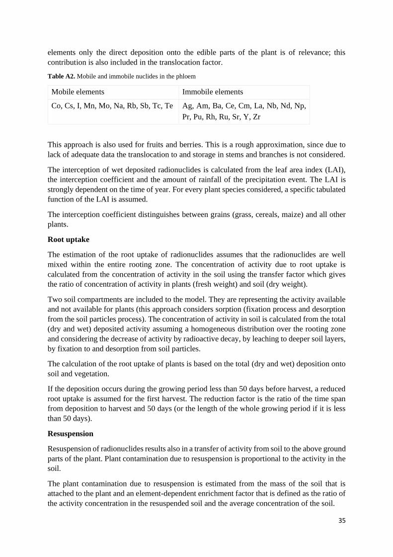
35
elements only the direct deposition onto the edible parts of the plant is of relevance; this
contribution is also included in the translocation factor.
Table A2. Mobile and immobile nuclides in the phloem
Mobile elements Immobile elements
Co, Cs, I, Mn, Mo, Na, Rb, Sb, Tc, Te Ag, Am, Ba, Ce, Cm, La, Nb, Nd, Np,
Pr, Pu, Rh, Ru, Sr, Y, Zr
This approach is also used for fruits and berries. This is a rough approximation, since due to
lack of adequate data the translocation to and storage in stems and branches is not considered.
The interception of wet deposited radionuclides is calculated from the leaf area index (LAI),
the interception coefficient and the amount of rainfall of the precipitation event. The LAI is
strongly dependent on the time of year. For every plant species considered, a specific tabulated
function of the LAI is assumed.
The interception coefficient distinguishes between grains (grass, cereals, maize) and all other
plants.
Root uptake
The estimation of the root uptake of radionuclides assumes that the radionuclides are well
mixed within the entire rooting zone. The concentration of activity due to root uptake is
calculated from the concentration of activity in the soil using the transfer factor which gives
the ratio of concentration of activity in plants (fresh weight) and soil (dry weight).
Two soil compartments are included to the model. They are representing the activity available
and not available for plants (this approach considers sorption (fixation process and desorption
from the soil particles process). The concentration of activity in soil is calculated from the total
(dry and wet) deposited activity assuming a homogeneous distribution over the rooting zone
and considering the decrease of activity by radioactive decay, by leaching to deeper soil layers,
by fixation to and desorption from soil particles.
The calculation of the root uptake of plants is based on the total (dry and wet) deposition onto
soil and vegetation.
If the deposition occurs during the growing period less than 50 days before harvest, a reduced
root uptake is assumed for the first harvest. The reduction factor is the ratio of the time span
from deposition to harvest and 50 days (or the length of the whole growing period if it is less
than 50 days).
Resuspension
Resuspension of radionuclides results also in a transfer of activity from soil to the above ground
parts of the plant. Plant contamination due to resuspension is proportional to the activity in the
soil.
The plant contamination due to resuspension is estimated from the mass of the soil that is
attached to the plant and an element-dependent enrichment factor that is defined as the ratio of
the activity concentration in the resuspended soil and the average concentration of the soil.

36
For grass and forage the soil intake of cattle is considered. This parameter is defined as the
amount of soil that is ingested by cattle per unit of grass or forage intake. Since during the soil
ingestion of animals, no fractionation occurs as during the resuspension, it is assumed that the
contamination of the soil ingested is equal to the mean activity in the soil. Therefore, the
enrichment factor is not applied. The resuspension and soil ingestion by cattle is formally used
as the transfer factor for root uptake.
Contamination of animal products
Primary contamination of animal products
The concentration of activity in animal products (milk, meat, and eggs) results from the intake
of activity by the animals, considering the kinetics of the radionuclides in the animal
metabolism.
The conceptual model of radionuclides interaction with cattle is shown below.
Figure A3. Conceptual model of the animal products
The amount of activity ingested by the animals is calculated from the concentration of activity
in the different feedstuffs. For the inhaled activity, the same transfer factor to animal products
as for ingested activity is assumed. This assumption is justified since for most elements the
same or very similar resorption factors for inhalation and ingestion is used in the metabolic
models for deriving dose conversion factors.
Plants or products processed from plants or animal products can be feedstuffs for animals. For
a realistic dose assessment in emergency situations, the feeding regimes must be adapted to the
season-dependent feed compositions of the specific region under consideration.
Ingestion of soil by grazing cattle is included in the feedstuff contamination. The soil intake of
animals is quantified in the model parameters by a factor which is defined as the amount of soil
(dry weight) per unit fresh weight of crop. This factor can be given for each of the plants
separately. It varies widely depending on the grazing management and the condition of the
pasture.
Inhalation of radionuclides by the animals is considered; this pathway may be relevant for early
contamination of animal products in certain cases (deposition during wintertime), but it is
relatively unimportant for the total resulting doses.

37
The time-dependent transfer to the animal products is described by the transfer factor fodder-
animal product and the retention function. The transfer factor fodder-animal product gives the
ratio of concentration of activity in the animal product and the daily intake of activity by the
animal for equilibrium conditions.
Change of activity concentration by storage and processing
The contamination of human foodstuffs and of the animals' fodder is calculated considering
the activity enrichment or dilution during processing and culinary preparation as well as
processing and storage times.
The concentration of activity decreases during storage and processing due to radioactive decay.
The contamination of the processed product is expressed by the processing factors which are
defined as the ratio of concentrations in the final processed product to that of the primary
product.
Calculation of doses by food ingestion
The intake of activity by the reference person is calculated from the time-dependent
concentrations of activity in foodstuffs and the human consumption rates.
Foodstuffs are assumed to be locally produced, i.e., the calculated ingestion doses represent
potential doses for people producing all their food locally. Age-dependent consumption rates
of the average population are applied.
Calculation of doses from occupancy
Doses from occupancy consider the following exposure pathways:
• Inhalation during cloud passage.
• External exposure due during cloud passage.
• Inhalation of suspended soil particles.
• External dose from radionuclides deposited on the ground.
• Exposure from contamination of closes and skin.
For calculation external dose from the ground, it is assumed that the deposited activity is
homogeneously distributed on an infinite meadow. Different deposition patterns and shielding
at different locations are taken into consideration by a correction factor.

38
Figure A4. Conceptual model for calculation of doses from occupancy
The following assumptions are made for calculations of doses from contamination of skin and
clothes:
• The deposition velocity for dry skin is same as for clothes. As default, a value of 1E-3
m s-1 is assumed.
• Indoors, the dry deposition is reduced by the factor which is also applied to estimate
the indoor inhalation dose.
• For the estimation of wet deposition on clothes and skin, the interception factor 0,1 is
applied. Wet deposition is only assumed for the time fraction people spent outdoors.
• For the fraction of the skin that is covered by clothes is set up to 0,8.
• The residence time of radionuclides on skin and clothes is the same. As default 24 h
hours are assumed. During this time, the activity is lost by radioactive decay only.
• The contamination of skin causes an exposure by alpha-, betta- and gamma-radiation,
whereas the contamination of clothes causes only an exposure due to gamma-radiation.
The dose factors for skin and clothes contamination were taken from Jacobi et al.
(1989). The values for skin represent the dose in skin averaged over a depth in skin of
50-100 µm.

39
Mathematical model
Input from atmospheric dispersion modelling
The contamination of soil is given by the sum of dry and wet deposition on soil. Total
deposition on soil is calculated by:
𝐴
soil total = Depo
soil,WET + Depo
soil,DRY
Where
Asoil total Total deposition on soil [Bq/m2];
Deposoil, WET Wet deposition on soil [Bq/m2];
Deposoil, DRY Dry deposition of nuclides on soil [Bq/m2];
Wet deposition on soil is calculated by:
Depo
soil,WET = Wet
deposition
Where
Wetdeposition Initial wet deposition [Bq/m2].
Dry deposition of nuclides on soil is calculated by:
Depo
soil,DRY = 𝐶
integrated,air ⋅ 𝑉
g,max,soil ⋅ seconds
per,hour
Where
Cintegrated, air The time-integrated activity concentration in air [Bq∙h/m3];
Vg, max, soil Maximum deposition velocity on soil [m/s];
secondsper, hour Conversion hours to seconds [s/h].
Maximum deposition velocity on soil is constant value (5.0 ∙ 10−4) for all nuclides, except
Iodine. For Iodine the next equation is used:
𝑉
g,max,soil[I] = 5.0 ∙ 10−4 ⋅ DV
soil,Particle + 0.003 ⋅ DV
soil,Elemental + 5.0 ∙ 10−5
⋅ DV
soil,Organic
Where
DVsoil Fraction of iodine in the form of particles, elemental and organic [unitless].
Mathematical equations for contamination of plants products
The initial contamination of the plants results from dry deposition onto the foliage of the plants
and from the fraction of wet deposition which is initially retained by the foliage.
𝐷𝑒𝑝𝑜 = 𝐷𝑒𝑝𝑜
𝐷𝑅𝑌 + 𝐷𝑒𝑝𝑜
𝑊𝐸𝑇
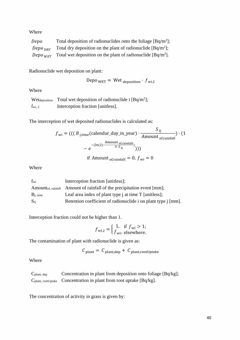
40
Where
𝐷𝑒𝑝𝑜 Total deposition of radionuclides onto the foliage [Bq/m2];
𝐷𝑒𝑝𝑜
𝐷𝑅𝑌 Total dry deposition on the plant of radionuclide [Bq/m2];
𝐷𝑒𝑝𝑜
𝑊𝐸𝑇 Total wet deposition on the plant of radionuclide [Bq/m2].
Radionuclide wet deposition on plant:
Depo
WET = Wet
deposition ⋅ 𝑓
wi,2
Where
Wetdeposition Total wet deposition of radionuclide i [Bq/m2];
fwi, 2 Interception fraction [unitless].
The interception of wet deposited radionuclides is calculated as:
𝑓
wi = ((( 𝐵
j,time (calendar_day_in_year) ⋅
𝑆
ij
Amount
of,rainfall ) ⋅ (1
− 𝑒−(ln(2)⋅
Amount
of,rainfall
3⋅ 𝑆 ij )
)))
if Amount
of,rainfall = 0, 𝑓
wi = 0
Where
fwi Interception fraction [unitless];
Amountof, rainfall Amount of rainfall of the precipitation event [mm];
Bj, time Leaf area index of plant type j at time T [unitless];
Sij Retention coefficient of radionuclide i on plant type j [mm].
Interception fraction could not be higher than 1.
𝑓
wi,2 = {
1,𝑓
wi ,
if 𝑓
wi > 1;
elsewhere.
The contamination of plant with radionuclide is given as:
𝐶
plant = 𝐶
plant,dep + 𝐶
plant,rootUptake
Where
Cplant, dep Concentration in plant from deposition onto foliage [Bq/kg];
Cplant, rootUptake Concentration in plant from root uptake [Bq/kg].
The concentration of activity in grass is given by:

41
𝐶
plant,dep (𝑡) =
𝐷𝑒𝑝𝑜
𝐸𝑔∙ {(1 − 𝑎𝑖) ∙ 𝑒−(𝜆𝑣𝑛+𝜆𝑤𝑖+𝜆𝑟) + 𝑎𝑖 ∙ 𝑒−(𝜆𝑡+𝜆𝑟)}
Where
𝐷𝑒𝑝𝑜 Total deposition of nuclide i on the grass [Bq/m2];
𝐸𝑔 Yield of grass at time of deposition (time-dependent) [kg/m2];
𝑎𝑖 Fraction of activity, which is translocated to the root zone [unitless];
𝜆𝑤𝑖 Weathering rate of nuclide i [d-1];
𝜆𝑣𝑛 Growth dilution rate dependent on the month of year [d-1];
𝜆𝑡 Rate constant representing translocation to the root zone and subsequent
remobilization [d-1];
𝜆𝑟 Radioactive decay constant [d-1].
For Type 2 and Type 3 the contamination at time of harvest is given by the initial contamination
at time of deposition, by loss of activity by weathering (by rain and wind):
𝐶
plant,dep (𝑡) =
𝐷𝑒𝑝𝑜
𝐸𝑗∙ 𝑒−(𝜆𝑤𝑖+𝜆𝑟)∙𝑡
Where
𝐷𝑒𝑝𝑜 Total activity of nuclide deposited on the foliage of plant, [Bq/m2];
𝐸𝑗 Yield of plant at time of harvest [kg/m2];
𝜆𝑤𝑖 Weathering rate of nuclide i [d-1];
𝜆𝑟 Radioactive decay constant [d-1].
For Type 4 and Type 5 plants the translocation of radionuclides from the leaves to the edible
part is considered as:
𝐶
plant,dep (𝑡) =
𝐷𝑒𝑝𝑜
𝐸𝑗∙ 𝑇𝑟𝑓(𝛥𝑡) ∙ 𝑒−𝜆𝑟𝑡
Where
𝐷𝑒𝑝𝑜 Total activity of nuclide deposited on the foliage of plant, [Bq/m2];
𝐸𝑗 Yield of plant at time of harvest [kg/m2];
𝑇𝑟𝑓(𝛥𝑡) Translocation factor for nuclide and plant type, depends on time 𝛥𝑡 between
deposition and harvest;
𝜆𝑟 Radioactive decay constant [d-1].
Concentration in grass from root uptake is calculated by:
𝐶
Plant rootUptake = 𝑇𝐹
𝑠𝑜𝑖𝑙,𝑝𝑙𝑎𝑛𝑡 ⋅ 𝐶
soil,total
Where

42
TFsoil, plant Transfer factor from soil to plant [unitless];
Csoil, total Total radionuclide activity in soil [Bq/kg].
Transfer factor from soil to plant includes root uptake, contamination of the plant by
resuspension and ingestion of soil by cows
TF
soil,plant = TF
rootUptake + 𝑓
e ⋅ 𝑅
j + 𝑆
j
Where
TFrootUptake Soil-plant transfer factor by root uptake [unitless];
fe Enrichment factor [unitless];
Rj Mass load of soil on plant [g/g];
Sj Soil intake by grazing animal [g/g].
The concentration of activity in soil is calculated from the total (dry and wet) deposited activity
assuming a homogeneous distribution over the rooting zone, and taking into account the
decrease of activity by radioactive decay, by leaching to deeper soil layers, by fixation to and
desorption from soil particles. The following analytical approach is applied:
𝐶
soil,total =
Depo
𝐿 ∙ 𝜌∙ [{𝑎𝑠 ∙ 𝑒−𝑏1∙𝑡 + (1 − 𝑎𝑠)𝑒−𝑏2∙𝑡} ∙ 𝑒−𝜆𝑟𝑡]
where
Depo Total deposition of radionuclides (dry + wet) on soil [Bq/m2];
𝑎𝑠 Coefficient representing distribution of nuclides in soil [unitless];
𝐿 Depth of rooting zone for pasture or arable soil [m];
𝜌 Soil density for pasture [kg/m3];
b1 and b2 Coefficients which represent loss processes [d-1].
Coefficient as is calculated by:
𝑎
s =
λ
fi − λ di
+ λ ai + RR
2 ⋅ RR
Where
λ
fi Fixation rate of nuclide i (pasture or arable soil) [d-1];
λ di Desorption rate of the nuclide i from the (pasture or arable) soil [d-1];
λ ai Leaching rate of nuclide i (pasture or arable soil) [d-1];
RR Coefficient [d-1].
Coefficients b1 and b2 are calculated by:
b1 =λ fi
+λ di +λ ai
+RR
2 and b2 =
λ fi +λ di
+λ ai −RR
2

43
Where
RR Coefficient [d-1].
The RR coefficient is calculated by:
RR = λ fi − λ di
+ λ ai 2 + 4 ⋅ λ fi
⋅ λ di
12
The grass model includes the production of hay: During another harvest period the average
contamination of fresh grass is calculated, and then multiplied by a factor of 5 (considering the
loss of water during hay preparation). The harvest period is subdivided into two intervals by
parameters giving the end of the first interval. During the first interval a weighting factor can
be defined considering the varying harvest intensity during the whole harvest period.
Example: If the harvest interval for hay is from 1st June till 30th September, the end of first
interval is 1st August, and the weighting factor of the first interval is 2, then it is assumed that
2/3 of the whole harvest is produced in the first half of the harvest period.
Radionuclide concentrations in hay:
Hay
= 5 ⋅ 𝑒−(time− Date
of deposition )⋅lambda
⋅ {Harvest
first,period ,
Harvest
second,period ,
if time
of,year >= 𝑡
harvest,begins 𝑎𝑛𝑑 time
of,year <= 𝑡
harvest,middle ;
elsewhere.
Concentration of radionuclides during first harvest period:
Harvest
first,period = Grass
Mean
Where
Harvestfirst, period Concentration gathered during harvest period [Bq/kg];
GrassMean Mean concentration of grass during harvest period [Bq/kg];
Mean radionuclide concentration in grass during harvest period:
Grass
Mean =
Grass Integrator
days
integrated

44
Where
Grass Integrator Preparation of grass during first harvest period which will be used for
production of hay[Bq];
daysintegrated Calculation of harvest interval length [d].
Harvest_second_period:
Harvest
second,period
= Grass
Mean,Snapshot + ( Grass
Mean − Grass
Mean,Snapshot ) ⋅ (1 −
weight
factor − 1
weight
factor + 1
)
Where
Harvestsecond, period RN concentration in grass during second period of hay preparation
[Bq/kg];
GrassMean, Snapshot Mean radionuclide concentration in grass at the middle of the harvest
period [Bq];
GrassMean Mean Rn concentration in grass during harvest period[Bq/kg];
weightfactor Weight factor for the first period for hay [unitless].
Mathematical equations for animal product contamination
Total activity concentration of radionuclides in animal products summed over biological
transfers is calculated as:
Farm
animals,products = ∑ Farm
products
Biological Transfer
Where
Farmproducts Activity concentration of radionuclides in animal products [Bq/kg].
Activity concentration of radionuclides in animal products is calculated as
Farm
products = TF
ik,farm ⋅ λ
bio,farm ⋅ Farm
products,corrected
where
TF
ik,farm Transfer factor fodder (farm animals) [d/kg];
λ
bio,farm Biological transfer rate [d-1];
Farmproducts, corrected Activity of radionuclides in farm products corrected by
animal time life [Bq].
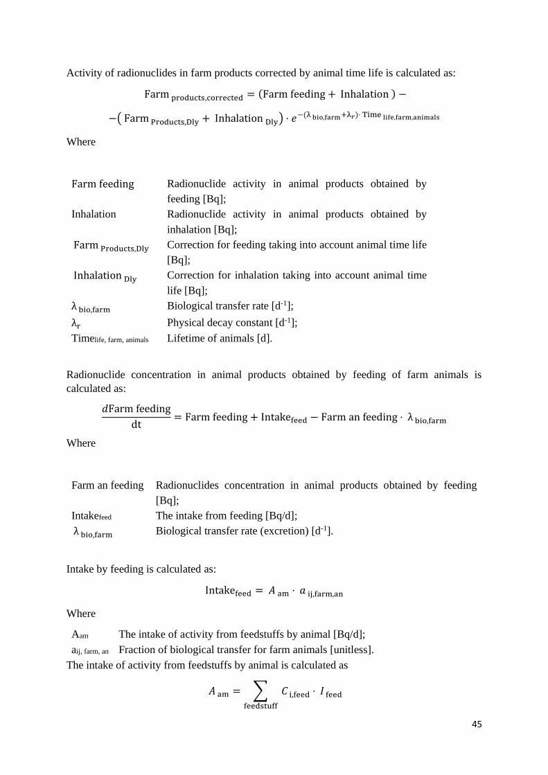
45
Activity of radionuclides in farm products corrected by animal time life is calculated as:
Farm
products,corrected = (Farm feeding + Inhalation
) −
−( Farm
Products,Dly + Inhalation
Dly ) ⋅ 𝑒−(λ bio,farm
+λ𝑟)⋅ Time
life,farm,animals
Where
Farm feeding Radionuclide activity in animal products obtained by
feeding [Bq];
Inhalation Radionuclide activity in animal products obtained by
inhalation [Bq];
Farm
Products,Dly Correction for feeding taking into account animal time life
[Bq];
Inhalation
Dly Correction for inhalation taking into account animal time
life [Bq];
λ bio,farm Biological transfer rate [d-1];
λr Physical decay constant [d-1];
Timelife, farm, animals Lifetime of animals [d].
Radionuclide concentration in animal products obtained by feeding of farm animals is
calculated as:
𝑑Farm feeding
dt= Farm feeding + Intakefeed − Farm an feeding ⋅ λ
bio,farm
Where
Farm an feeding Radionuclides concentration in animal products obtained by feeding
[Bq];
Intakefeed The intake from feeding [Bq/d];
λ
bio,farm Biological transfer rate (excretion) [d-1].
Intake by feeding is calculated as:
Intakefeed = 𝐴
am ⋅ 𝑎
ij,farm,an
Where
Aam The intake of activity from feedstuffs by animal [Bq/d];
aij, farm, an Fraction of biological transfer for farm animals [unitless].
The intake of activity from feedstuffs by animal is calculated as
𝐴
am = ∑ 𝐶
i,feed ⋅ 𝐼
feed
feedstuff

46
Ci,feed Concentration of activity of radionuclide i in feedstuff [Bq/kg];
Ifeed Intake rate of feedstuff by the farm animal [kg/d].
Radionuclide activity in animal products obtained by is calculated as:
𝑑Inhalation animals
dt= Inhalation animals + Intakeinhalation − Inhalation animals
⋅ Lambda
bio,farm
Where
Inhalation animals Radionuclide activity in animal products obtained by inhalation [Bq];
Intakeinhalation Intake by feeding [Bq/d];
Lambda
bio,farm Biological transfer rate [d-1].
Intake by inhalation for animal is calculated as:
Intakeinhalation = A nimal inhalation
⋅ 𝑎
ij,farm,an
Where
𝑎
𝑖𝑗,𝑓𝑎𝑟𝑚,𝑎𝑛 Fraction of biological transfer for animal product [unitless].
Activity of radionuclides inhalated by animal during cloud passage (24 hours) is calculated as:
Animal
inhalation = 𝐶
integrated,air ∙ Inhrate
Where
Animalinhalation Activity of radionuclides inhalated by animal [Bq];
Cintegrated,air The time-integrated activity concentration in air [Bq∙h/m3];
Inhrate Inhalation rate of animal k [m3/h].
Storage and processing of foodstuff and feedstuff
In case of time after deposition is lower than storage time concentration in foodstuff is equal
to 0.
The concentration of activity decreases during storage and processing due to radioactive decay
𝐶
RN,After,Storage = 𝐶
iq ⋅ 𝑒−λ𝑟⋅ 𝑡
storage,processing
Where
CRN, After, Storage Concentration of activity of radionuclide i in foodstuffs or feedstuff at
time t after processing and storage [Bq/kg];
Ciq Concentration of activity of RN i in the processed product q [Bq/kg];
λ𝑟 Physical decay constant [d-1];

47
𝑡
storage,processing Storage and processing time of food- or feedstuff [d].
The contamination of the processed product is expressed as:
𝐶
iq = 𝑉
ipq ⋅ Concentration
raw product p
Where
𝑉
ipq Processing factor of nuclide i for production of the processed
product q from the primary products p [unitless];
Concentration
raw product p Activity concentration in raw product p (cropland plants,
animal farm products and plants) [Bq/kg].
Effective dose from foodstuff ingestion
Radiation exposure due to ingestion of the foodstuff for referenced person is calculated as:
𝑑Dose
dt= Concentration
for,ingestion ⋅ 𝑉
n ⋅ DCC
ing,food ⋅ mSvperSv
Where
Dose Radiation exposure due to ingestion of the foodstuff n [mSv];
Concentrationfor,
ingestion
Radionuclide i concentration in foodstuff n after storage and processing
[Bq/kg];
Vn Consumption rate of foodstuff n at time t [kg/d];
DCCing, food Dose conversion factor for ingestion of nuclide i at time t [Sv/Bq];
mSvperSv Amount of mSv in 1 Sv [mSv/Sv];
hoursper, day Conversion days to hour [h/d].
Effective dose from ingestion of foodstuff summed over the radionuclides is calculated as:
Dose
ingestion,RN,food = ∑ Dose𝑅𝑛
𝑛
𝑖=1
Where
DoseRn Dose from ingestion of foodstuff contaminated by nuclide i
n Number of radionuclides

48
Doses from occupancy
Dose from inhalation during cloud passage
The dose Doseinh, cloud due to inhalation of radionuclides during the passage of the radioactive
cloud is calculated from the time-integrated activity concentration in the near ground air, the
inhalation rate, and the age-dependent dose factor for inhalation In addition, a reduction factor
can be applied taking into account the lower activity in air inside houses:
Dose
inh,cloud = 𝐶
integrated,air ⋅ 𝐼 ⋅ DCC
inh,cloud ⋅ 𝑟
inh,summ,cloud ⋅ mSvperSv
Where
Doseinh, cloud Inhalation dose [mSv];
Dateof, first, deposition Date when deposition happened [d];
Cintegrated, air The time-integrated activity concentration in air [Bq*h/m3];
I Age-dependent inhalation rate [m3/h];
DCCinh, cloud Dose conversion factor for inhalation of radionuclide i
[Sv/Bq];
rinh, summ, cloud Summed reduction factor for staying indoors [unitless];
mSvperSv Amount of mSv in 1 Sv [mSv/Sv].
Summed reduction factor for staying indoors:
𝑟
inh,summ,cloud = ∑ 𝑟
inh
Locations
Where
rinh Reduction factor for staying indoor [unitless].
Reduction factor for staying indoor
𝑟
inh = 𝑓
ui ⋅ 𝑐
Lij,cloud
Where
rinh Reduction factor for staying indoor [unitless];
fui Relative occupancy time at location j during passage of
cloud [unitless];
cLij, cloud Filtering factor for nuclide i and environment j [unitless];

49
Dose from external exposure during cloud passage
External exposure from radionuclides in the cloud is calculated by:
𝐷
w,i = 𝐶
integrated,air ⋅ DCC
external,cloud ⋅ 𝑟
w,i,summ ⋅ mSvperSv
Where
Dw,i External exposure from radionuclides in the cloud [mSv];
Cintegrated, air The time-integrated activity concentration in air [Bq·h/m3];
DCCexternal, cloud Dose factor for external exposure from cloud [Sv·m3·Bq-1·h-1];
rw, i, summ Summed reduction factor [unitless];
mSvperSv Amount of mSv in 1 Sv [mSv/Sv];
The summed reduction factor:
𝑟
w,i,summ = ∑ 𝑟
w,i
Locations
Where
rw, i Reduction factor for staying at different locations [unitless].
Reduction factor for staying at different locations:
𝑟
w,i = 𝑓
ui ⋅ 𝑐
wij
Where
rw, i Reduction factor for staying at different locations [unitless];
fui Relative occupancy time at location j during passage of cloud [unitless];
cwij Environment factor for cloud exposure at location j [unitless].
Dose of external exposure from the ground
Dose from radionuclides in the ground is calculated by:
𝑑Dose ext ground
dt= Dose ext ground + Ground
depo,time ⋅ 𝑟
bi,summ ⋅ DCC
external,ground
⋅ seconds
per,hour ⋅ hours
per,day ⋅ mSvperSv,
Where
Dose ext ground Dose from radionuclides in the ground [mSv];
Dateof, first, deposition Date of deposition [d];
Grounddepo, time Total deposition on ground as function of time [Bq/m2];

50
rbi, summ Reduction factor for staying at different locations
[unitless];
DCCexternal, ground Age dependent dose factor for exposure from ground
(Sv/s)*(m3/Bq) [GSF-12/90][Sv*m2*Bq-1*s-1];
secondsper, hour Conversion hour to seconds [s/h];
hoursper, day Conversion days to hour [h/d];
mSvperSv Amount of mSv in 1 Sv [mSv/Sv].
Reduction factor for staying at different locations:
𝑟
bi,summ = ∑ 𝑟
bi
Locations
Where
rbi Reduction factor for staying at different locations[unitless]
Reduction factor for staying at different locations:
𝑟
bi = 𝑓
ui ⋅ 𝑐
bij
Where
rbi Reduction factor for staying at different locations [unitless];
fui Relative occupancy time at location j during passage of cloud [unitless];
cbij Environment factor for cloud exposure at location j [unitless].
Total deposition on ground (soil + lawn) as function of time is calculated by
Ground
depo,time = Lawn
depo,total ⋅ (
a1
lambda
1 + lambda
⋅ (𝑒−( lambda
1 +lambda)⋅(time− Date
of,first,deposition −1)
− 𝑒−( lambda
1 +lambda)⋅(time− Date
of,first,deposition )
Where
Grounddepo, time Total deposition on ground as function of time [Bq/m2];
Dateof, first, deposition Date of deposition [d];
Lawndepo, total RN total deposition on lawn [Bq/m2];
a1 Contribution fractions of the migration rates [unitless];
lambda1 Migration rates [d-1];
lambda Physical decay constant [d-1];
a2 Contribution fractions of the migration rates [unitless];
lambda2 Migration rates [d-1].

51
Radionuclides total deposition on lawn that is used in external exposure calculations.
Lawn
depo,total = Depo
soil,TOTAL + Lawn
Dry,deposition
Where
Lawndepo, total RN total deposition on lawn[Bq/m2]
Deposoil, TOTAL Total deposition Bq/m2[Bq/m2]
LawnDry, deposition Dry deposition onto lawn [Bq/m2]
Dose in organ k due to skin contamination
Dose in organ k due to skin contamination is calculated by:
Dose
in,organ,from,skin,contamination = (𝐶
integrated,air ⋅ seconds
per,hour ⋅ 𝑉
g,H ⋅ 𝐶
H + 𝑓
H,N
⋅ Wet
deposition ⋅ 𝑓
F ) ⋅ DCC
Skin,to,organs ⋅ 𝐴
H ⋅ (
1 − 𝑒−lambda⋅
𝑡
H
hours
per,day
lambda)
⋅ seconds
per,hour ⋅ hours
per,day ⋅ mSvperSv
Where
Dosein, organ, from, skin, contamination Dose in organ k due to skin contamination [mSv];
Cintegrated, air The time-integrated activity concentration in air [Bq*h/m3];
secondsper, hour Conversion hour to seconds [s/h];
Vg, H The deposition velocity for dry skin [m*s-1];
CH Reduction factor for staying indoors [unitless];
fH, N Interception factor [unitless];
Wetdeposition Wet deposition activity [Bq/m2];
fF Fraction of time spent outdoors [unitless];
DCCSkin, to, organs Dose rate in the organ k after skin contamination [Sv*s-1/Bq];
AH Total area of skin [m2];
lambda Physical decay constant [d-1];
tH Skin exposure time [h];
hoursper, day Conversion days to hour [h/d];
mSvperSv Amount of mSv in 1 Sv [mSv/Sv].
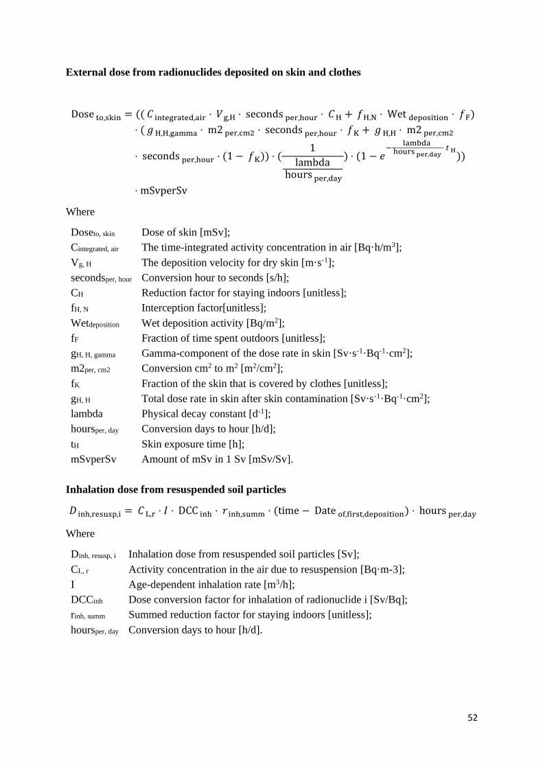
52
External dose from radionuclides deposited on skin and clothes
Dose
to,skin = (( 𝐶
integrated,air ⋅ 𝑉
g,H ⋅ seconds
per,hour ⋅ 𝐶
H + 𝑓
H,N ⋅ Wet
deposition ⋅ 𝑓
F )
⋅ ( 𝑔
H,H,gamma ⋅ m2
per,cm2 ⋅ seconds
per,hour ⋅ 𝑓
K + 𝑔
H,H ⋅ m2
per,cm2
⋅ seconds
per,hour ⋅ (1 − 𝑓
K )) ⋅ (
1
lambdahours
per,day
) ⋅ (1 − 𝑒−
lambdahours
per,day ⋅ 𝑡
H
))
⋅ mSvperSv
Where
Doseto, skin Dose of skin [mSv];
Cintegrated, air The time-integrated activity concentration in air [Bq·h/m3];
Vg, H The deposition velocity for dry skin [m·s-1];
secondsper, hour Conversion hour to seconds [s/h];
CH Reduction factor for staying indoors [unitless];
fH, N Interception factor[unitless];
Wetdeposition Wet deposition activity [Bq/m2];
fF Fraction of time spent outdoors [unitless];
gH, H, gamma Gamma-component of the dose rate in skin [Sv·s-1·Bq-1·cm2];
m2per, cm2 Conversion cm2 to m2 [m2/cm2];
fK Fraction of the skin that is covered by clothes [unitless];
gH, H Total dose rate in skin after skin contamination [Sv·s-1·Bq-1·cm2];
lambda Physical decay constant [d-1];
hoursper, day Conversion days to hour [h/d];
tH Skin exposure time [h];
mSvperSv Amount of mSv in 1 Sv [mSv/Sv].
Inhalation dose from resuspended soil particles
𝐷
inh,resusp,i = 𝐶
L,r ⋅ 𝐼 ⋅ DCC
inh ⋅ 𝑟
inh,summ ⋅ (time − Date
of,first,deposition ) ⋅ hours
per,day
Where
Dinh, resusp, i Inhalation dose from resuspended soil particles [Sv];
CL, r Activity concentration in the air due to resuspension [Bq·m-3];
I Age-dependent inhalation rate [m3/h];
DCCinh Dose conversion factor for inhalation of radionuclide i [Sv/Bq];
rinh, summ Summed reduction factor for staying indoors [unitless];
hoursper, day Conversion days to hour [h/d].
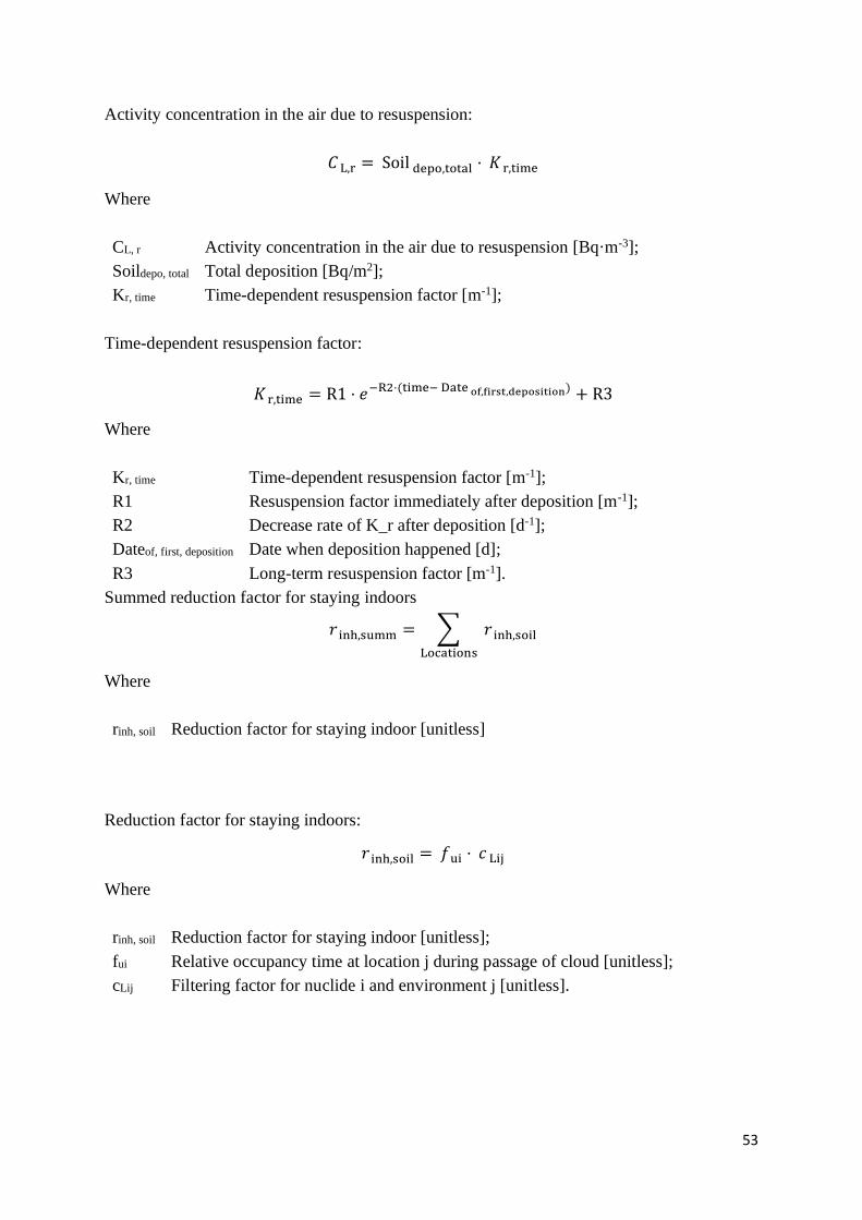
53
Activity concentration in the air due to resuspension:
𝐶
L,r = Soil
depo,total ⋅ 𝐾
r,time
Where
CL, r Activity concentration in the air due to resuspension [Bq·m-3];
Soildepo, total Total deposition [Bq/m2];
Kr, time Time-dependent resuspension factor [m-1];
Time-dependent resuspension factor:
𝐾
r,time = R1 ⋅ 𝑒−R2⋅(time− Date
of,first,deposition ) + R3
Where
Kr, time Time-dependent resuspension factor [m-1];
R1 Resuspension factor immediately after deposition [m-1];
R2 Decrease rate of K_r after deposition [d-1];
Dateof, first, deposition Date when deposition happened [d];
R3 Long-term resuspension factor [m-1].
Summed reduction factor for staying indoors
𝑟
inh,summ = ∑ 𝑟
inh,soil
Locations
Where
rinh, soil Reduction factor for staying indoor [unitless]
Reduction factor for staying indoors:
𝑟
inh,soil = 𝑓
ui ⋅ 𝑐
Lij
Where
rinh, soil Reduction factor for staying indoor [unitless];
fui Relative occupancy time at location j during passage of cloud [unitless];
cLij Filtering factor for nuclide i and environment j [unitless].

Bibliographic Data Sheet NKS-449
Title EcoFood - A tool for assessment of radiation exposure in
terrestrial environments impacted by airborne releases
Author(s) Hosseini, A.1, Avila, R2., Hryhorenko, D.2, Brown, J.1,
Peltonen, T.3, Virtanen, S.3, Nielsen, S.4, Gudnason, K5.
Affiliation(s) 1DSA (Norway), 2AFRY (Sweden), 3STUK(Finland), 4DTU(Denmark), 5IRSA (Iceland)
ISBN 978-87-7893-541-0
Date June 2021
Project NKS-B / ECOFOOD
No. of pages 52
No. of tables 10
No. of illustrations 11
No. of references 29
Abstract The software package FDMT - Food Chain and Dose Module
for Terrestrial Pathways is a component of the decision support
systems, JRODOS and ARGOS, that are currently used in the
Nordic countries for response to nuclear emergencies. Not all
food chains that are relevant for the Nordic conditions are
currently supported by FDMT and the modelling of some of the
food chains is not optimal for the Nordic conditions, resulting
in difficulties with the parameterization of the models.
Moreover, in its current implementation FDMT is not totally
transparent to users. The focus of the project was to develop a
new software (EcoFood) that addresses these deficiencies and
considers the findings of a gap analysis of FDMT conducted
early in the project. The report presents the findings of the gap
analysis, provides an overview of EcoFood´s components: the
Simulator, the Model Library and the Parameter Database and
a discussion on improvements and advantages inherent to
EcoFood.
Key words radionuclide, releases, atmospheric, environment, terrestrial,
dose, humans
Available on request from the NKS Secretariat, P.O.Box 49, DK-4000 Roskilde, Denmark.
Phone (+45) 4677 4041, e-mail [email protected], www.nks.org


![kCnifjp;%& II - NCERTdksfdys & nks dks;y two cuckoos,rs & ;s (f}opu] L=kh-) these pVosQ & nks xkSjS;k two sparrows oqQ#r% & djrh gSa do fogjr% & iqQnd jgh gSa hopping pkfyosQ & nks](https://img.pdfslide.net/doc/110x75/613280cadfd10f4dd73a7dfa/kcnifjp-ii-ncert-dksfdys-nks-dksy-two-cuckoosrs-s-fopu.jpg)