Embed Size (px)
Citation preview
AD-A1 7 0 NAVAL POSTGRADUATE SCHOOL MONTEREY CA F/6 13/6
NMEIRICAL OPTIMIZATION FOR INTERNAL EXPANDING BRAKE.UUUCL E MAR 81 M PEERNCLASSIFIEO NL
mmhhhhhhmmhmENumIIIIEEIhIhIEElEElllllElhlhIIIIIIIIIIIIIIIIIIIIIIIIIIIIu*IIIIIIIIIIIIIIN
NAVAL POSTGRADUATE SCHOOLMonterey, California
• t!
THESISNUMERICAL QPTIMIZATION FORINTERNAL EXPANDING BRAKE
by
" ,XORDECHA I/ PEER
MarelIM81 - //
Thesis Advisor: G. N. Vanderplaats
Approved for public release; distribution unlimited
L\ - •
SECURITY CLASSIFICATION Of THaIS P"6 fRon D.EWm.
REPOR DOCUMENTATION PAGE 8*3 OAD COMPLETINORM1. REPORT NMUER jGOVT ACCESSION NO. 3. RECIPIENT'S CAOGK~~ HUON
4. TIL.Krm subttle)S. TYP or REPORT 6 PERIOD COVERED
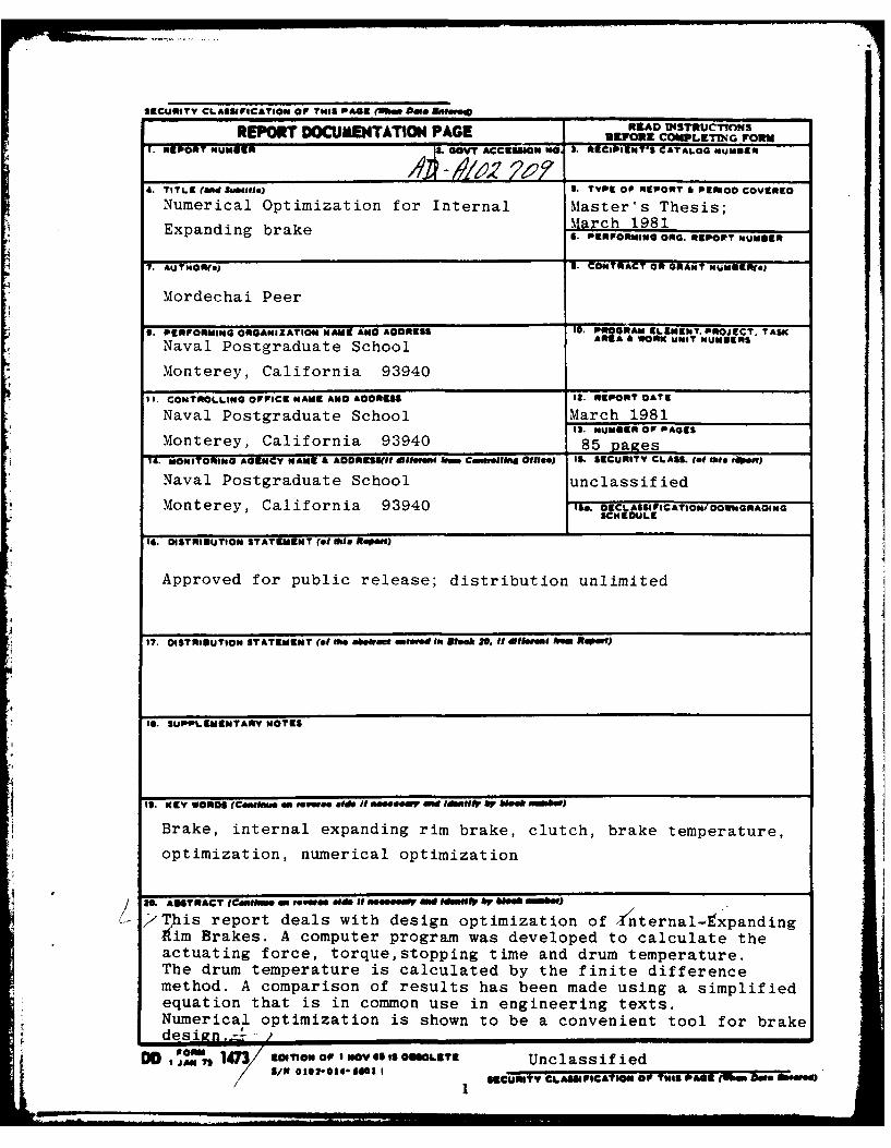
Numerical Optimization for Internal Master's Thesis;Expanding brake March 1981
S. PERFORMING ONG. 41EPoPT NMB~ER
7. AUTHOR(*) 9. CONTRACT OR GRNA-T NuMSERt(.J
Mordechai Peer
9. PERFORMING ORGANIZATION HNK AND ORESS 10- ROGAM ELEMENT. PROJECT. TASKAREA & WORK UNIT NUMBERS
Naval Postgraduate School
Monterey, California 93940
11. CONTROLLING OFFICE NAME ANC ADDRESS 12. REPORT DATS
Naval Postgraduate School March 1981IS. NUMBER OFPAGES
Monterey, California 93940 8 ae1.MONITORING AGENCY NAME A AOESS(Ol dlff e 11MM Conevoljgin Office) S6. SECURITY CLASS. (of thee ,fuW)
Naval Postgraduate School unclassified
Monterey, California 93940 IS&. 01CLSI IC ATION/OWN GRAING
14. DISTRIBUTION STATEMENT (Of11114 flePO)
* Approved for public release; distribution unlimited
17. DISTRIBUTION STATEMENT (of the abstrat 40100 lot D*..h It f gre. 1mm RaPit)
IS. SUPPLEMENTARY NOTES
19. KEY WORDS (Cnens et reverse side ifoneser aw *miftr AV ee UMAube')
Brake, internal expanding rim brake, clutch, brake temperature,optimization, numerical optimization
20. ABSTRACT (Cm.Umm 40 eeOW01* a11411 81 00ee..eY aiirb Melb 1411001aA,)
/This report deals with design optimization of tinternal-txpandingIfim Brakes. A computer program was developed to calculate theactuating force, torque,stopping time and drum temperature.The drum temperature is calculated by the finite differencemethod. A comparison of results has been made using a simplifiedequation that is in common use in engineering texts.Numerical optimization is shown to be a convenient tool for brake
DO I 147 EITION OPPIMOV 69I1SOBSLETE Unclassified
SECURITY CLASSIFICATION OFP TNIS PAGE (Whose mlos
Approved for public release; distribution unlimited.
Numerical Optimization forInternal Expanding Brake
by
Mordechai PeerMajor, Israeli Army
B.Sc. Technion, Haifa Israel, 1970
Submitted in partial fulfillment of therequirements for the degree of
MASTER OF SCIENCE IN MECHANICAL ENGINEERING
From the
NAVAL POSTGRADUATE SCHOOL
March 1981
Author: A c- A c oh.
Approved by: .bod 44 Ad~,h 7 iL4S
Thesis Advisor
3 eaeSecond Reader
Chairman, partment of! ;cal Engineering
. -. Dean of Science and Engineering
2

ABSTRACT
This report deals with design optimization of Internal-
Expanding Rim Brakes. A computer program was developed to
calculate the actuating force, torque, stopping time and
drum temperature. The drum temperature is calculated by the
finite difference method.
A comparison of results has been made using a simplified
equation that is in common use in engineering texts.
Numerizal optimization is shown to be a convenient tool
for brake design.
Accesion For _
nTI S GRA&IDTIC TA ElUnannounced L
4f4 to---
D i t r Ibui I,./_-
Av.iiabl-i'tY CodesAkvra iln/or
3Special
3I

TABLE OF CONTENTS
I. INTRODUCTION ..................- 11
II. INrERNAL-EXPANDING RIM CLUTCHES AND BRAKES -12
A. GENERAL MECHANICAL PRINZIPLES-------------- 12
B. FRICTION FUNDAMENTALS AND MATERIALS----------12
C. BRAKE DRUMS ---------------------------------- 13
D. STATIC AND DYNAMIC ANALYSIS ------------------- 14
1. Assumptions ----------------------------- 14
2. Pressure Concept --------------------------- 143. Actuating Force and Torque Calculation----15
4. Rate of Heat Generated and Deceleration---17
E. SURFACE TEMPERATURE CALCULATION--------------- 18
1. Assumptions ------------------------------- 19
2. Temperature Analysis ---------------------- 19
a. Thegry -------------------------------- 19b. Formulation --------------------------- 20
F. BRAKE DUTY CYCLE ------------------------------ 21
III. OPTIMIZATION -------------------------------------- 22
A. INTRODUCTION ---------------------------------- 22
B. DEFINITION OF TERMS ------------------------ 23
C. THE OPTIMIZATION PROCESS-24
D. COPES AND SUBROUTINE PN&LIZ- 26
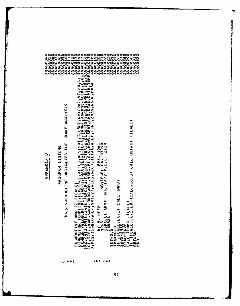
IV. DESCRIPTION OF THE PROGRAM------------------------27
A. GENERAL PROGRAM ORGANIZATION ------------------ 27
B. SUBROUTINES ----------------------------------- 27
1. Subroutine ANALIZ------------------------- 27
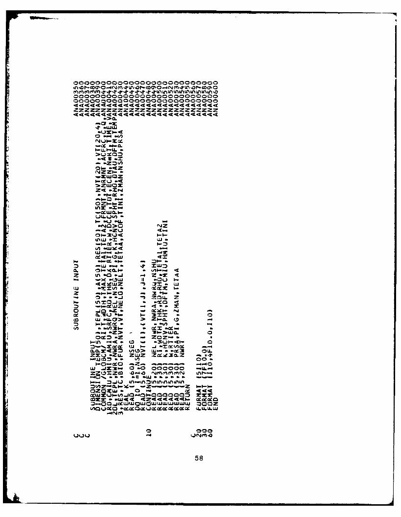
2. Subroutine INPUT -------------------------- 27
3. Subroutine TEMP--27
4. Subroutine TEMA --------------------------- 28
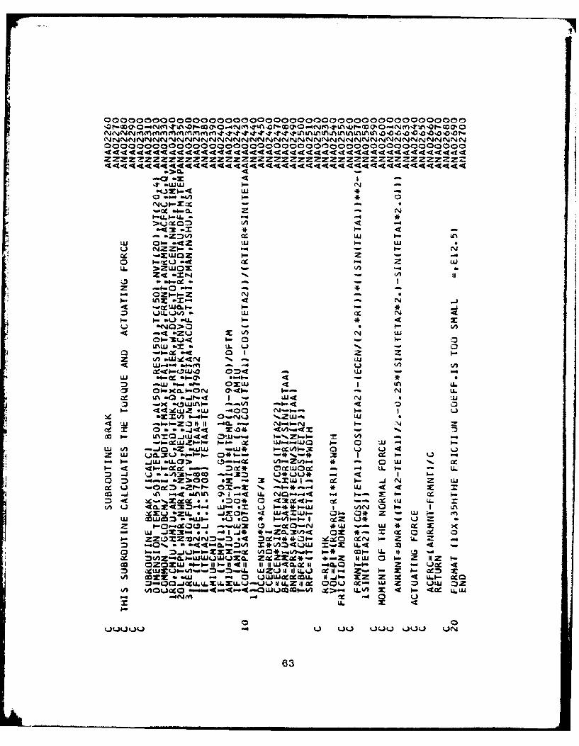
5. Subroutine BRAK --------------------------- 286. Subroutine OUTPUT---------.......-28
V. TESr PROBLE AND RESULTS-.........-29
VI. TEMPERATURE RAISE-SI&PLIFIED CALCULATION ---------- 32
4

VII. CONCLUSIONS- 314
VIII. RECOMENDATIONS FOR FUTURE INVESTIGATION ....-. 34
APPENDIX k: LIST Of PARAdETERS --- 47
APPENDIX B: INSTRUCTIONS FOR PROBLEM DECK PREPARATION--50
APPENDIX Z: STANDARD DECK STRUCTURE----------------------53
appendix D: COMPUTER PROGRAM LISTING--57
APPENDIX E: FIGURES ------------------------------------ 65
LIST OF REFERENCES -------------------------------------- 83BIBLIOGRAP---------------------------84
INITIAL DISTRIBUTION LIST ------------------------------- 85
5
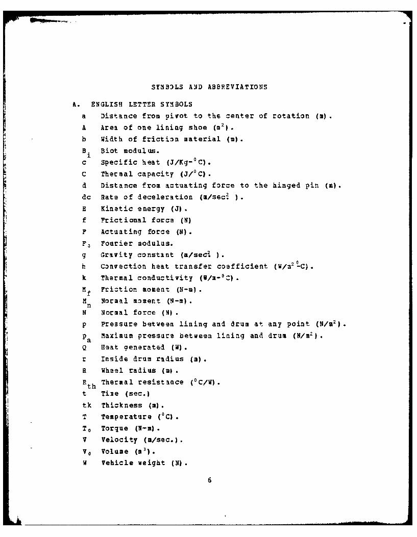
SYMB2LS AND ABBREVIATIONS
A. ENGLISH LETTER SY4BOLS
a Distance from pivot to the center of rotation (m).
A Are& of one lining shoe (M2,.
b Width of friction material (m).
B. Biot modulus.1
c Specific heat (J/Kg- °C).
C Thermal capacity (J/C).d Distance from actuating force to the hinged pin (m).
dc Rate of deceleration (m/sec. ).
E Kinetic energy (J).
f Frictional force (N)
F Actuating force (N).F0 Fourier modulus.
g Gravity constint (m/sec2 ).
h Convection heat transfer coefficient (W/32 IC).
k Thermal conductivity (W/m-OC).
Mf Friction moment (N-m).
M Normal moment (N-m).nN Normal force (N).
p Pressure between lining and drum at any point (N/I2 ).
Pa Maximum pressure between lining and drum (N/m2}.
Q Heat generated (W).
r Inside drum radius (m).
R Wheel radius (mi.
Rth Thermal resistance (°C/W).
t Tize (sec.)
tk Thickness (m).
T Temperature ('C)
T0 Torque (N-m.
V Velocity (m/sec.).
V0 Volume (M3').
W Vehicle weight (N).
6
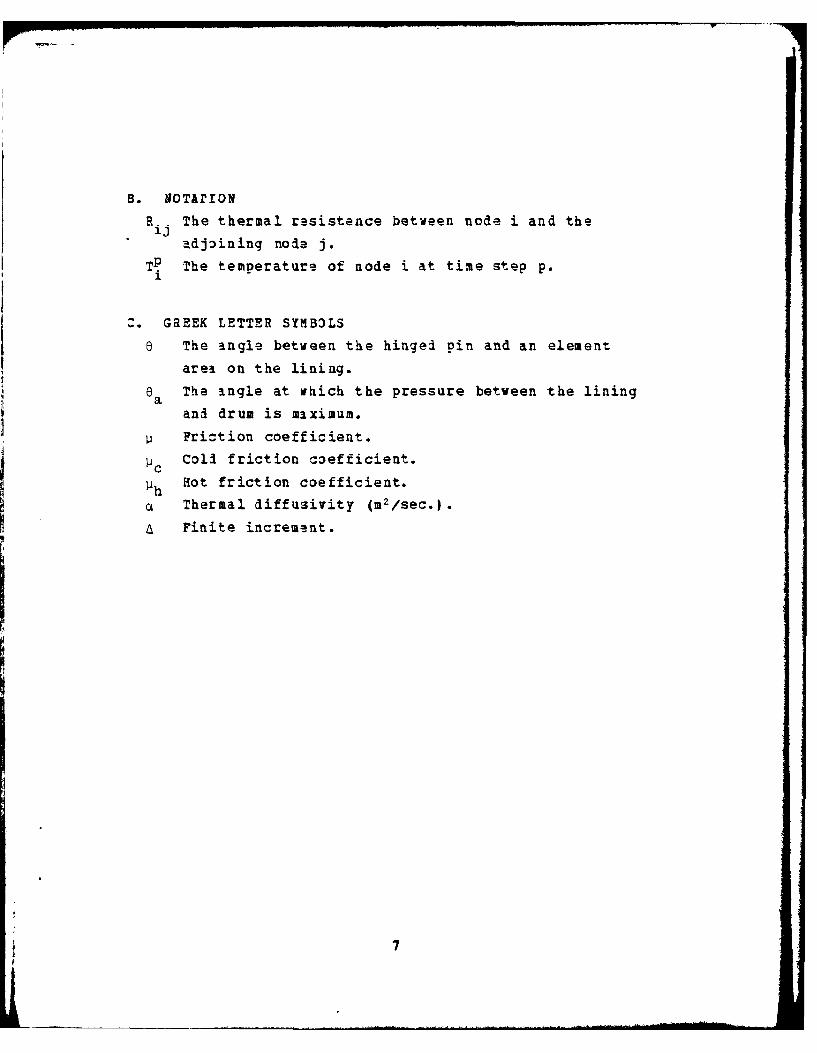
S. NOTA'ION
R.. The thermal resistance between node i and theij
adjoining node J.TP The temperature of node i at time step p.
1
GREEK LETTER SYMBOLS
e The angle between the hinged pin and an element
area on the lining.
6 The angle at which the pressure between the lininga
and drum is maximum.
U Friction coefficient.
1c Coll friction coefficient.
11h Hot friction coefficient.
c Thermal diffusivity (m2/sec.).
A Finite increment.
7
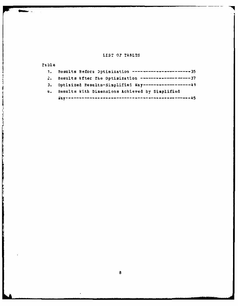
LIST 0? TABLES
Table
1. Results Befora Jptimization ---------------------- 35
2. Results hfter The Optimization-....-373. Optimized Results-Simplifiel Way ------------------ 41
4. Results With Dimensions Achieved by Simplified
Way------------------------------------------------ 45
8

LIST OF FIGURES
Figure1. Dynamic Representation of a Brake-65
2. Brake Assembly -----------------------------------66
3. Finite Difference Model of the Drum-67
4. Blozk Diagram of the Program68
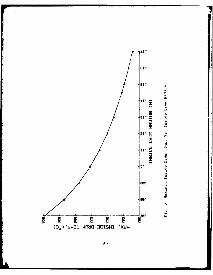
5. Maximum Inside Drum Temperature Vs. Inside Drum
Ralis -------------------------------------------- 69
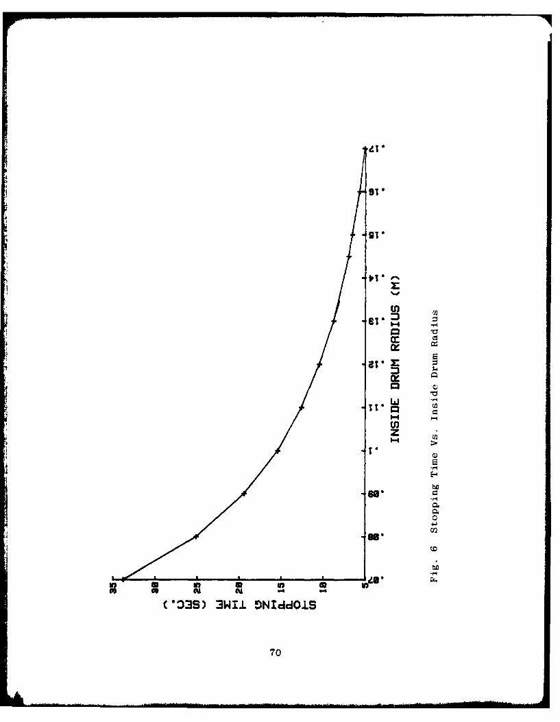
6. Stopping Time Vs. Inside Drum Radius-------------70
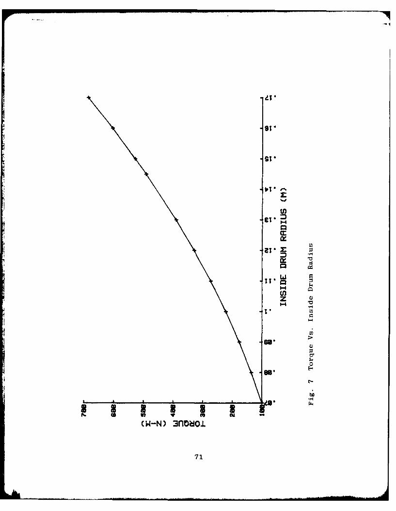
7. Tocgue Vs. Inside Drum aadius-.....-71
8. Maximum Inside Drum Temperature Vs. Drum Width----72
9. Stopping Time Vs. Drum Width --------------------- 73
10. Torque Vs. Drum Width ----------------------------- 74
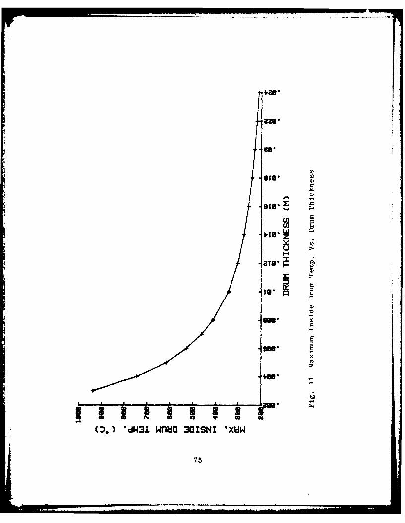
11. Maximum Inside Drum Temperature Vs. Drum
Thizkness ----------------------------------------- 75
12. Sto.ping Time Vs. Drum Thickness ----------------- 76
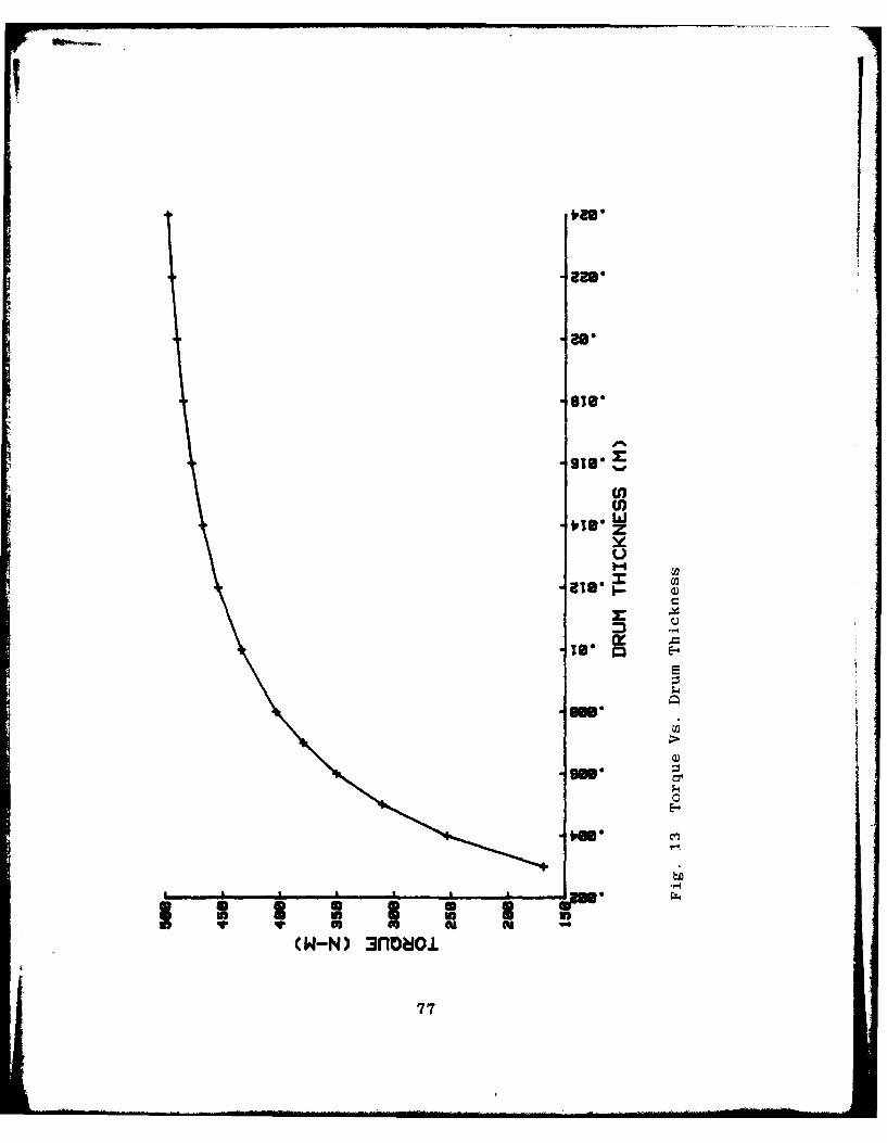
13. Torque Vs. Drum Thickness ----------------- 77
14. Maximum Inside Drum Temperature Vs. Theta2---------78
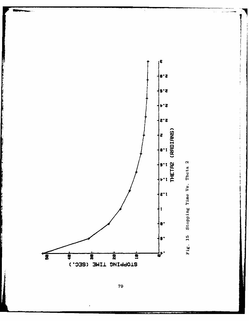
15. Stopping Time Vs. Theta2 ----------------------- 79
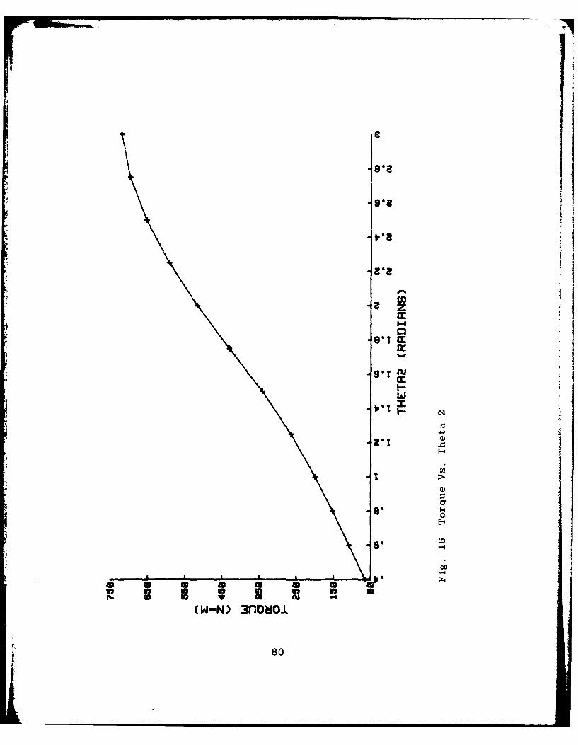
16. Torque Vs. Thet12--------------------------------- 80
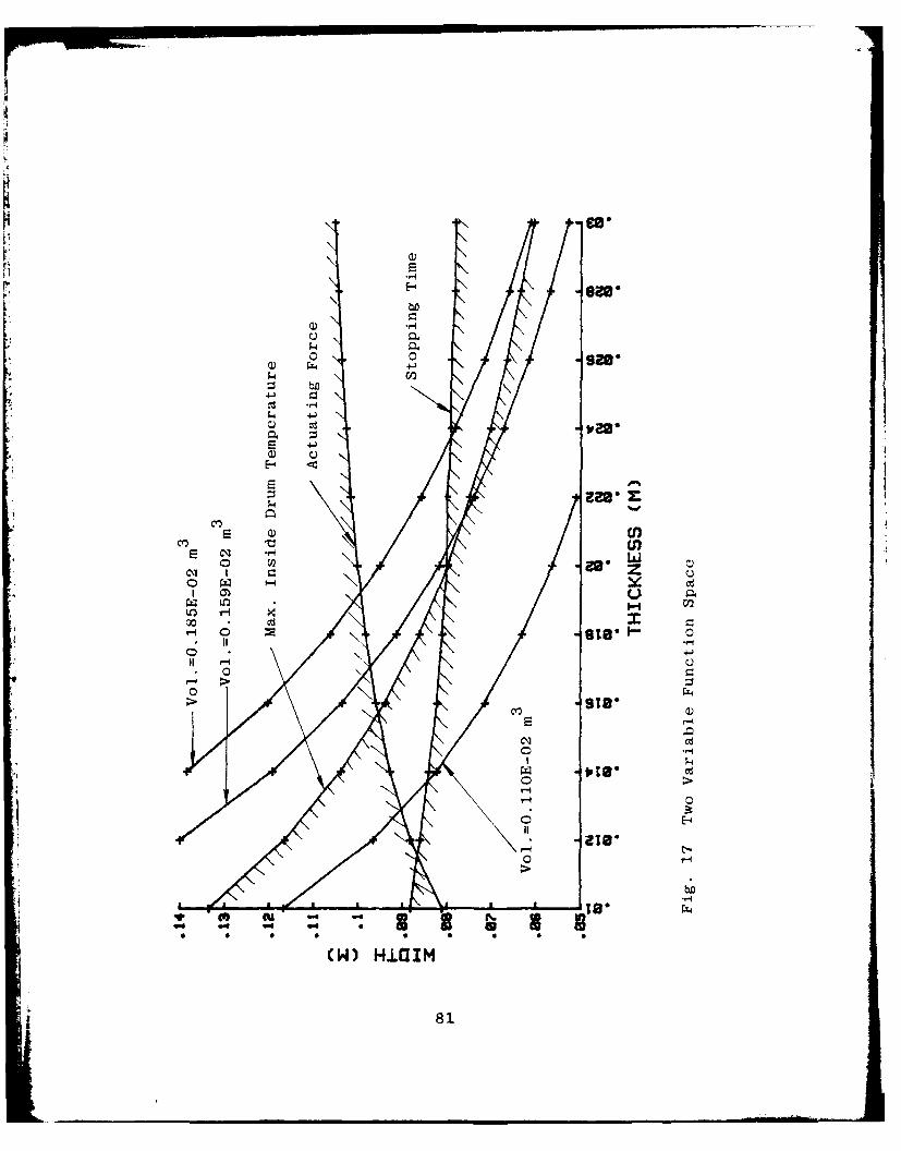
17. Two Variable Function Space-Width and Thickness---81
18. Drum Temperature Vs. Time-Zomparison--------------82
9
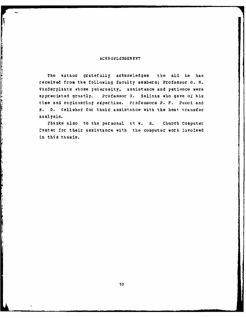
ACKNOWLEDGEMENT
The aathor gratefully acknowledges the aid he has
received from the following faculty members; Professor G. N.
Vanderplaits whose generosity, assistance and patience were
appreciated greatly. Professor D. Salinas who gave of his
time and enginsering expertise. Professors P. F. Pucci and
M. D. Kelleher for their assistance with the heat transfer
analysis.
Thanks also to the personal at W. R. Church Computer
Zenter f o their assistance with the computer work involved
in this thesis.
10
I. INTRODUCTION
Brakes are mechanical devices for retarding the motion
of a vehicle or machine by means of friction. Because of the
similarity of their functions, many clutches may also be
included here, assuming centrifugal forces are accounted
for.
A simplified dynamic representation of a brake is shown
in Fig. 1. Two masses with inertias, I, and 12 r rotating
at the respective angular velocities w, and W 2 (one of which
may be zero), are to be brought to the same speed by
engaging the brake.
The friction brake has three basic elements; two
opposing friction surfaces and a mechanism for forcing the
friction surfaces into contact. Whenever a friction brake is
eagaged to Join two members having relative motion, there is
a period of slip which may last several seconds. This slip
is one of the chief merits of the friction brake; i: absorbs
siocks iad prevents excessive torsicnal stresses on the
power transmission system. On the other hand, slip is the
limiting factor in friction clutch and brake performance;
for heat is generated in proportion to slip, torque
transmitted, and period of slip.
The following parameters are of interest in analyzing
the performance of these devices;
1. The actuating force.
2. The torque transmitted.
3. The temperature rise.
4. The 3lip time.
This report deals with Int-rnal-Expanding Rim Brakes.
This formulation also applies to internal-expanding clutches
if centrifugal forces are accounted for.
LI
II. INTERNAL-EXPANDING RIN CLUTCHES AND BRAKES
A. GENERAL MACHANICAL PRINCIPALS
A brake or clutch assembly, uses a brake shoe to which
is attached a friction material, called lining. The liningis riveted or bonded to the brake shoe as shown in Fig. 2.
The brake shoe is pivoted at a fiKed point and the other end
is subjected to a force which presses the shoe in contact
with the drum. The force between the brake and the drum is
radial as the drum rotates. If a point on the rotating drum
surface first makes contact with the shoe at the end nearest
the pivot, the shoe is termed a "trailing shoe". If it first
makes contact at the other end the shoe is termed "leading
shoe,, the latter giving a higher braking torque than the
former for a given braking force.
The friction between the lining and the drum creates
heat which is basically the conversion of energy of motion
of the vehicle or machine to thermal energy at the friction
surfaces, namely the lining and the drum. This heat is then
dissipatel and absorbed by the drum by conduction,
convectioa and radiation into the atmosphere.
B. FRicrroN FUNDAMENrALS AND IATESIALS
Friction mechanisms, such as brakes, are systems for
converting mechanical energy into heat. Several basicfactors affect friction and wear of materials used in brake
systems. The main factors are temperature, pressure, speed,
surface roughness, and type of material. Some organic or
molded friction materials show no change in friction
characteristics with pressure, while others such as
sintered-metal materials decrease in friction coefficient as
pressure is increased. For metallic friction materials there
is also a decrease in coefficient of friction as speed
12
increases. Temperature effects upon the coefficient of
friction vary widely with the type of materials used.
In a two-shoe internal expanding brake there is a
tendency for the brake drum to deform under hard
application. Drums become elliptical and the force to do
this is guite high and contributes to friction force.
A brake or clutch friction material should have the
following characteristics to a legree which is dependent
upon the severity of the service:
1. A high and uniform coefficient of friction.
2. The ability to withstand high temperatures, together
with good heat conductivity.
3. Properties which are not affected by environmental
conditions such as moisture.
4. Good resiliency.
5. High resistance to wear, scoring and galling.
C. BRAKE DRUMS
One of the primary functions of a brake drum is that of
absorbing and dissipating the heat developed during the
application of the brake. A brake drum is a heat sink into
which heat goes after it is created by the rubbing friction
of the brake lining contact to drum. The brake shoe and
lining permanently fixed on the axle, when actuated,
contacts the drum under pressure to cause the friction to
stop the vehicle. The energy of motion of a vehicle is
converted to thermal energy bj the brake assemblies. A brake
drum must have the capacity to absorb and dissipate this
heat energy within the limits of the brake heat input. If
this is not the case, the drum expands and the brakes fade
or fail. The greater the mass of the drum, the more heat it
can absorb and store until such time as the heat can be
dissipated by convection and radiation [Ref. 1].
An ideal brake drum would have the following
characteristics;
13
1. High structural strength to resist bursting forces.
2. Uniform coefficient of friction.
3. Hard surface to resist scoring.
4. High heat conductivity to rapidly conduct heat away
from braking surfaces.
5. High emissivity factor to radiate heat from the drum
surface to the atmosphere.
6. High heat storage capacity to store heat from
successive brake applications until it can be
dissipated.
7. Good aachinability to permit boring of the drum.
D. STATIZ AND DYNAMIZ ANALYSIS
1. Assumptions
In developing the equations, the following
assumptions have been made;
a. The pressure at any point on the shoe is proportional
to the moment arm of this point from the pivot.
b. The effect of centrifugal force may be neglected.
c. The shoe is assumed to be rigid.
d. The friction coefficient is a linear function of
temperature and it does not vary with pressure, wear
and environment.
2. Pressure Concept
ro analyze an internal shoe refer to Fig. 2, which
shows a shoe pivotel at a fixed point with the actuating
force acting at the other end of the shoe. The mechanical
arrangement does not permit pressure to be applied at the
pivot, therefore the pressure at this point is zero. If the
shoe rotates through a small angle about A, the radial
movement of any point on the arc of contact, is proportional
to the moment arm of this point from the pivot. Assuming
that the material of the brake lining and support obey
Hooke's law, the pressure at this point will also be
proportional to this moment arm. The distance is
14
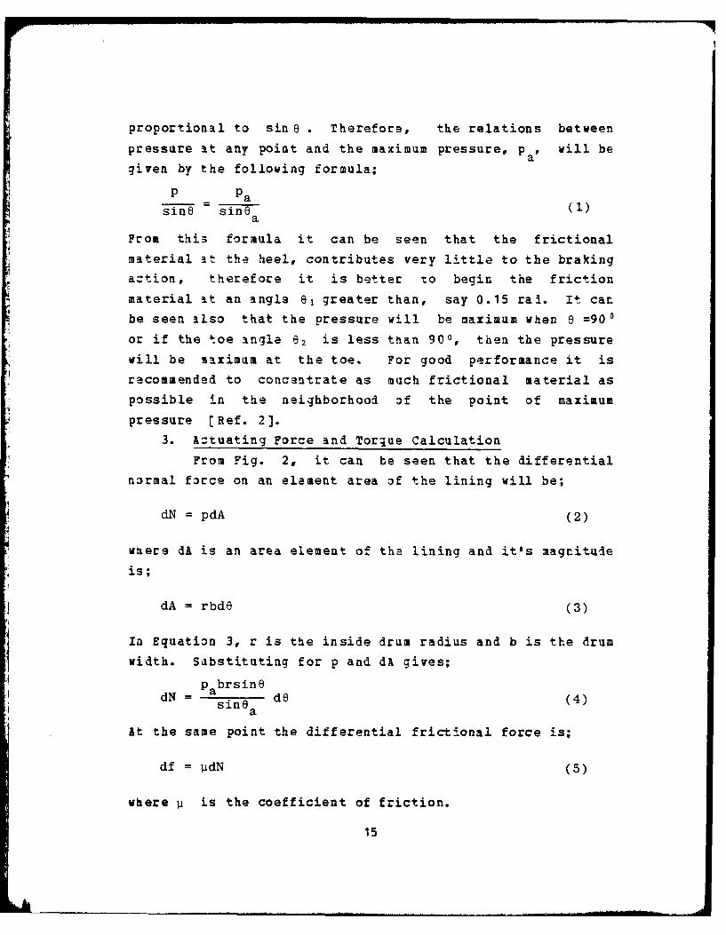
proportional to sin e . Therefore, the relations between
pressure at any point and the maximum pressure, pa' will be
given by the following formula;
P PasinG- sine (1)
a
From this formula it can be seen that the frictional
material at the heel, contributes very little to the braking
action, therefore it is better to begin the friction
material it an angle 61 greater than, say 0.15 ral. It can
be seen also that the pressure will be maximum when 8 =900
or if the toe angle 02 is less than 900, then the pressure
will be maximum at the toe. For good performance it is
recommended to concentrate as much frictional material as
possible in the neighborhood of the point of maximum
pressure [Ref. 2].
3. Actuating Force and Torque Calculation
From Fig. 2, it can be seen that the differential
normal f3rce on an eleament area of the lining will be;
dN = pdA (2)
where dA is an area element of the lining and it's magnitude
is;
dA = rbde (3)
In Equation 3, r is the inside drum radius and b is the drum
width. Sabstituting for p and dA gives;dN4 pabrsin(
dN a sine de (4)a
At the same point the differential frictional force is;
df = UdN (5)
where U is the coefficient of friction.
15
A..
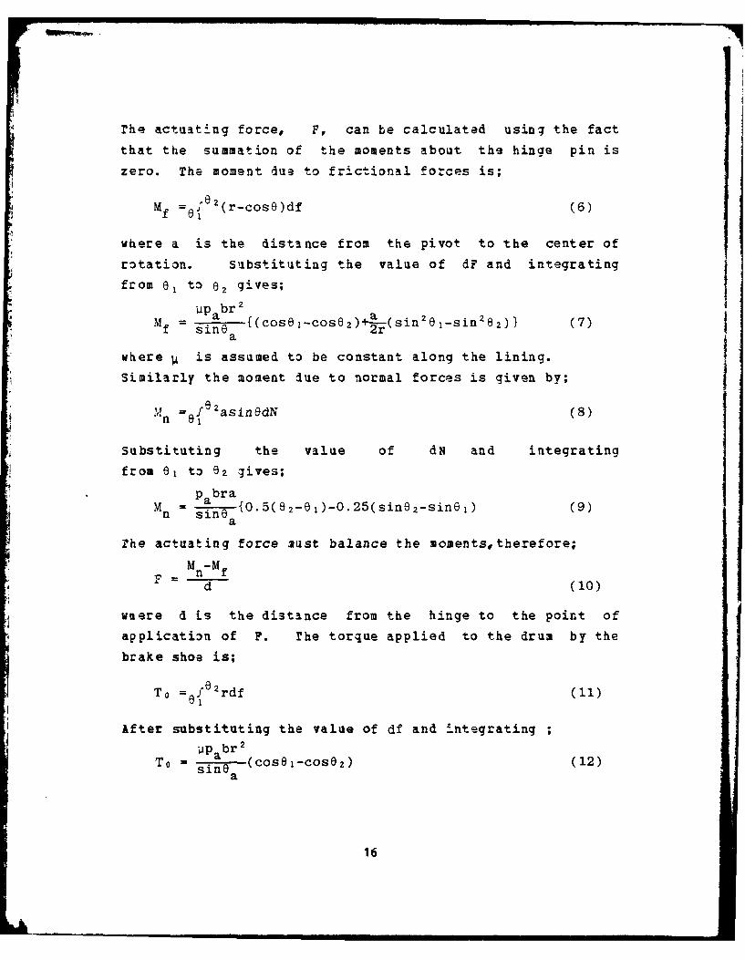
rhe actuating force, F, can be calculated using the fact
that the summation of the moments about the hinge pin is
zero. The moment due to frictional forces is;
Mf =ef 2(r-cos0)df (6)
where a is the distance from the pivot to the center of
rotation. Substituting the value of dF and integrating
from el to 02 gives;
Mf = siae {(cos8 1-cos 2 )+ r(sin201- sin28 2 )} (7)
f sine 2a
where is assumed to be constant along the lining.
Similarly the moment due to normal forces is given by;
M = OeasinedN (8)n
Substituting the value of dN and integrating
from e to 82 gives;pabra
Mn = sinea-{0.5(6 2-01 )-0.25(sin6 2-sin01 ) (9)siOa
rhe actuating force must balance the moments,therefore;
Mn-Mnf
d (10)
where d is the distance from the hinge to the point of
application of F. rhe torque applied to the drum by the
brake shoe is;
= fe2rdf (11)
After substituting the value of df and integrating ;
To = sine (cose-cos6z) (12)sinea
16

4. Rate of Heat 3enerated and Deceleration Calculation
The differential rate 3f heat generated by an
element area of the lining is equal to the velocity of the
inside surface of the drum relative to the lining , times
the differential frictional force acting on the element
area;
dQ = V df (13)r
Assuming the brake is on a vehicle wheel with a radius of R,
the inside surface velocity is equal to;
V V (14)r R
where V is the velocity of the vehicle and is a function of
time.
If V=V(t) then V =V (t) and the heat generated will be alsor ra functi3 of time. Substituting the values of V and df and
rintegrating from ei to 82 , we get the following formula for
the heat generated at any time t,
P bu 2a rQ(t) = sin ()(cosei-cose 2)v(t) (15)
4 . The kinetic energy of a vehicle of weight W is given by;
E =(.)v (16)
Note that if the brake is on a four wheel vehicle, there
will be eight shoes. Assuming all are leading shoes, each
will stop one-eight of the vehicle weight, so W/8 must be
used in Eguation (161. The rate of change in the kinetic
energy is;
dE ,W ddE (E) V~ (17)
From the energy conservation law the rate of change in the
kinetic energy is equal to the heat generated;
17
Q(t) dE (18)
Substituting the value of Q(t) aad dE/At, it is seen that
the velocity V(t) cancels and so the deceleration is not a
function of time. Therefore the deceleration, dc, is;
dV _ P a r-dc = dt (W sine()(COSel-cos6 2 ) (19)
The velocity at any time is;
V = V.-dct (20)
where Vi is the initial velocity. Substituting the velocity
i. Equation (16), yields the rate of heat generated as afunction of time,
Pabl4rP bP 2
Q(t) (-)(cose1-COSe 2 )(Vi-dct) (21)a
Ia this study the friction coefficient was taken as constant
up to a temperature of 900C and after 90 0C, decreases
linearly to zero at a specified temperature, Tmax;
T <90 C
P --E - (T-90) 90 0C < T < T (22)
0 T >Tmax.
where p is the cold coefficient of friction and Ph is the
hot coefficient of friction.
E. SURFAZE TEMPERATURZ CALCULATION
Since the function of a brake is to convert kinetic
energy into heat, surface temperatures of brake linings and
drums are most important. Therefore it is necessary to know
the temperature of the mechanism during and after any stop.
The temperatures were calculated by the finite difference
method.
18
1. Assumptionsa. One dimensional heat flow-The heat flow is from the
inner surface to the outer surface of the drum.
b. Constant heat transfer coefficient.
C. No heat dissipated by radiation.d. The heat is generated on the inner surface.
2. remperature Analysis
a. Theory
The differential equation to be solved in order
to find the temperature in the drum, based on the
assumptions, is;
2 = TT (23)
with the following boundary conditions:
at 1=0 heat is generated,
at x=tk heat is transferd to the atmosphere by
convection.
In the equation above k is the thermal conductivity, a is
the ther2al diffusivity, t is time and tk is the drum
thickness. This .luation can be solved by the finite
difference method "Ref. 3]. The finite difference model
used here is shown in Fig. 3. The rate of change with time
of the internal energy of a node i is approximated by;TP'lTP
AE _ ocVo 1 (24)At At
where p is the density, c is the specific heat and V0 is
the drum volume.
Now define the thermal capacity as
Ci = Dici AVoi (25)
rhe forward difference equation for all nodes and boundary
conditions is;
19
TP-T P TP TPRJ 1 C 1 (26)R th, ij i At
where th,ij is the thermal resistance
Solving the above equation for TP+ 1 gives;1TP A
p+l= (QpMR A 1 )TP (27)th,ij C i Rth,ij
The thermal resistance can be calculated from the geometry
and boundary conditions "Ref. 3]. To ensure
stability At must be equal or less than the following
nodal relation;C
At < ( ) (28)
th ij
With the assumptions made, the drum can be viewed as an
infinite plate, with heat generated at the surface of the
first node, as shown in Fig. 3. it is assumed that in every
drum, there are two shoes and that both are leading shoes.ptherefore, two times QP must be taken.
TP~l TP(2Qi J + (1- )TP (29)
th,ij 1 i th,ij
b. Formulation
In the computer program 5 nodes were taken. In
order to :heck accura-y, the program was run with 7 and 10
nodes. in each case the result was the same within 5 0C.
rhe heat is generated in the inner drum surface. Therefore Q
appears in the formula of temperature in the first node and
fir all the other nodes Q is equal zero. With the
assumptions mentionel above, the heat transfer through the
drum is solved as a heat transfer problem through an
infinite plate, with heat generation at the inner surface
aad with a heat convection boundary on the outer surface as
shown in Fig. 3. Equation (29) =an be simplified using two
dimensionless parameters, Biot and Fourier modulii,
20
B. = hAx (30)i k
FO aAt (31)(Ax) r
The final equations for calculating the temperatures at the
nodes now become;
For the first node;
Tl 1 2QPAtP+- C1 + (1-2Fo)TP + 2FGTP (32)
For the interior nodes;
TPl p + Tp + (1 2)TP} (33)i ~ ~ 1 0T_ +1 FO
For the last node;
T P+I - 2Fo{TP +B.T.+ (..-B.-l)TP} (34)n n- 1~ 2F 0 i nl
F. BRAKE DUTY CYCLE
In addition to tae parameters mentioned above the design
of a brake depends on the initial speed, final speed, number
of stops, and the rest time between each stop. In this
analysis a general daty cycle was considered so that the
initial speed, final speed ani the acceleration period
between stops can be different for each part of the design.
In the design examples presented here, a vehicle was
stopped four consecutive times with the following cycle;
Initial final Rest
Speed Speed
m/sec. a/sec. sec.
1 25.0 0.0 20.0
2 25.0 0.0 20.0
3 25.0 0.0 20.0
4 25.0 0.0 -
21

III. OPTIMIZATION
A. INTRODUCTIOV
Engineering analysis using the digital computer has
become commonplace. It is less common to use the computer
to make the actual design lecisions, such as sizing of
structural members or placement of mechanical linkages. This
may be largely attributed to the fact that fully automated
design requires techniques that ire unfamiliar to much of
the engineering community.
In many engineering problems, it is necessary to
determine the minimum or maximum of a function of several
variables, limited by various linear and nonlinear
inequality constraints. It is seldom possible, in practical
applications, to solve these problems directly, and
iterative methods are used to obtain the numerical solution.
Machine calculation of this solution is, of course,
desirable. The CON3IN program is available to solve a wide
variety of such problems [Ref. 4].
C03MIN is a FORTRXN program, in subroutine form, for theminimization of a multi-variable function subject to a set
of inequality constraints. The basic optimization algorithm
is the Method of Feasible Directions (Ref. 5]. The user must
provide a main calling program and an external routine to
evaluate the objective and constraint functions and to
provide gradient information. tf analytic gradients of the
objective or constraint functions are not available, this
information is calculated by finite difference. While the
program is intended primarily for efficient solution of
constrained problems, unconstrained function minimization
problems say also be solved, and the Conjugate Direction
Method of Fletcher and Reeves is used for this purpose
[Rqf. 6].
22

B. DEFINITION 3? TERMS
Most lisciplines have a unique set of nomenclature used
to describe the concepts within that discipline. Some of the
commonly sed terms in numerical optimization are summarized
here.objective- rha value of the function which is to be
minimized or maximized during the optimization process.
Synonyms ire cost, merit and payoff. The common mathematical
designation is F(X). In the present study the objective was
to minimize the material in the brake drum.
Design variables- Thi parameters to be changed
during the optimization process in order to minimize or
maximize the value of the objective function. Synonym;
decision variables. rhe common mathematical designation is
the vector X. Design variables considered in this study
include, drum thickness, width, the angle between the hinged
pin and the end of the lining, and the distance from the
pivot to the center of rotation.
Inequality constraints- one-sided conditions which
must be mathematically satisfied for the design to be
acceptable. The common mathematical term is G(X)<O or
G(X)>O. If the ineqality condition is satisfied on G(X), the
design is acceptable, (feasible). If it is not satisfied,
the design is not acceptable (infeasible) . Constraints
considered here include, vehicle stopping time, maximum drum
temperature, and actuating force.
Side constraints- Upper and lower bounds on the
individual design variables X . The common mathematical
representation is X .< Ii< Xi.
Design space- The n-dimensional mathematical space
spanned by the vector of design variables I.
&ctive constraint- Constraint G. (X) is called active3if its value is zero (or near zero for computational
purposes.
23
Inactive constraint- Constraint G. (X) is inactive if
JJG.(X)< O.
7iolated constraint- Constraint G (X) is violated if
3, (X) >0.J
C. THE JPTIHIZATION PROCESS
The general design optimization problem can be stated
mathematically as follows: Find the set of variables Xi,
i=1,2....a, which willminimize F(. (35)
Subject to:
Gj(X) < 0 j=1,2 ..... m (36)
X 1< X. < Xu i=1,2 ..... n (37)
Vector X contains the set of independent design
variables X., i=1,2....n. X may represent, for example1
width, thickness, and angles in the brake optimization. The
objective function used here is the drum volume.
Equation (36) defines the ineqality constraints imposed
on the design. For example, if the temperature on the inner
drum surface must not exceed a specified value T, the
associeted design constraint becomes, in normalized form
T 1 < 0 (38)Ti
The lower and upper bounds on the design variables,
given by Eq. (37) , limit the region over which the functions
F(X), and G(X) are defined. These constraints are often
referred to as side constraints because they form the sides
or bounds of the n-dimensional spaced spanned by the design
variables K.
If all the inequalities of Eqns. (36) and (37) aresatisfied, the design is said to be feasible; if any ofthese conditions are not satisfied, the design is not
24

feasible. If F(X) is a minimum and the design is feasible,
it is also optimum, or at least, a relative optimum. Note
that because the objzztive and constraints may be nonlinear,
there may be multiple minima in the design space that cannot
be identified using current methods. While this is a matter
for concern, since it is desired to find the true optimum,
it must be remembered that the same mathematical conditions
exist if the design process is not automated. However, using
optimization techniques, it is a simple matter to restart
the optimization from several initial points in the design
space and thereby improve the pribability of obtaining the
true optilum design, a process that would be quite time-
consuming in manual design.
Equations (35)-(37) define the nonlinear constrained
optimization problem. If Eqs. (361 and (37) are not imposed
on the design, the optimization problem is defined by
Ej.(35) aLone and is therefore an unconstrained minimization
problem.
Most 2onlinear optimization algorithms 1pdate the vector
of design variables by the iterative relationship;
Rq = Rq-1 + agq (39)
where q is the iteration number, vector S is the direction
of search in the design space, and the scalar a is referred
to as a aive parametar which,together with 9, determines how
such the vector i is changed luriag the q-th iteration. An
initial design defined by i must be supplied. The
optimization process then proceeds in two steps. First,
the direction S, whizh improves the design, is found, and
second, the scalar a , is determined which improves the
design as much as possible when moving in this direction.
rhe process is repeated until there is no further design
improvement, indicating that this is the optimum attainable
25
design. ?ir further details see Ref. 7.
D. COPES AND SUBROUTINE ANALIZ
In order to simplify the use of CONMIN and to further
aid in the design optimization process a Control Program For
Engineeriag Synthesis, COPES, was developed by Vanderplaats
[Ref. 7]. COPES is the main program (recall that CONMIN is
written in subroutine form). The user must supply an
analysis subroutine with the name ANALIZ, which will
calculate the various parameters. This subroutine has three
segments; INPUT, EXECUTION, OUTPUr.
All parameters which may be d9sign variables, objective
functions or constraints are contained in a single labeled
common block called GLOBC3.
Copes Terminology
The OPPES program currently provides six specific
capabilities;
1. Simple analysis, just as if ZOPES was not used.
2. Optimization-Minimization or maximization of one
calculated function with limits imposed on other
functions.
3. Sensitivity analysis- The effect of changing one or
more design variables on one or more calculated
fun:tions.4. Two-variable function space-knalysis for all specified
combinations of two design variables.
5. Optiaum sensitivity- The same as sensitivity analysis
except that, at each step, the design is optimized with
respect to the independent design variables.
6. Approximate optimization- Optimization using
approximation techniques. Usually more efficient than
standard optimization for up to 10 design variables or
if multiple optimizations are to be performed (Ref. 7].
26

IV. DESCRIPTION OF TKE COMPUTER PROGRAM
A. GENERAL PROGRAM ORGANIZATION
A functional block diagram of the program is presented
in Fig. 4. A general description of the subroutines
contained in the program is given here. Appendices A
t.rough D discuss the preparation of input data, list the
important computer program nomenclature, and list the
program.
B. SUBROU7INES
1. Subroutine ANALIZ
Subroutine ANALIZ organizes the basic analysis used
in the optimization. It controls the reading of the initial
design Jescription and calculation of the values of the
objective function, constraints, and all other parameters
necessary to solve the problem. COPES/COUHIN updates the
design to minimize/maximize the objective function,
iterating until no further iprovement in the objective
fanction is possible without violating one of the
constraints. COPES/CONMIN calls subroutine ANALIZ to obtain
the function value luring the optimization.
2. Subroutine INPUT
rhis subroutine reads all input data associated with
the brake analysis. Instructions for problem deck
preparation are given in appendix B.
3. Subroutine rE.PR
rhis subroutine calculates the heat transfer
constants such as the thermal capacity of each node and the
resistance of each node, determines the time increment in
order to insure a stable solution, and calculates the rate
of heat generation. In order to calculate the temperature of
each node, it calls two subroutines. From subroutine BRAK it
27

obtains the deceleration needed to calculate the rate of
heat gemn.ratel and from subroutine TEMA it obtains the
temperature rise of each node. Then it calculates the
temperatur-s during the time that the brake is not in use.
This subroutine is also c.apble of calculating the
temperature rise of a drum when a constant rate of heat
dissipation is given.
4. Subroutine rEIA
This subroutine calculates the temperature of each node.
As mentioned before, the heat is generated on the inner
s:irface, and on the outer side of the drum the heat is
dissipated by convection. The formulas used were developed
by the finite difference method, and are given in sectionII-E-2.
5. Subroutine BRAK
This subroutine calculates the torque, actuating force,
aad the friction moment of one shoe. It also calculates the
drum volume and the decelerat-ion of the machine. The
subroutine takes into consideration a constant friction
coefficient until a temperature of 90 0C is reached and a
linear decrease in the friction coefficient for higher
temperatures. More details are given in section II-D-4.
6. Subroutine 3UTPUT
This subroutine echos the input data and prints out
the thermal and meahanical information for the brake. An
example of the output obtained from this subroutine is shown
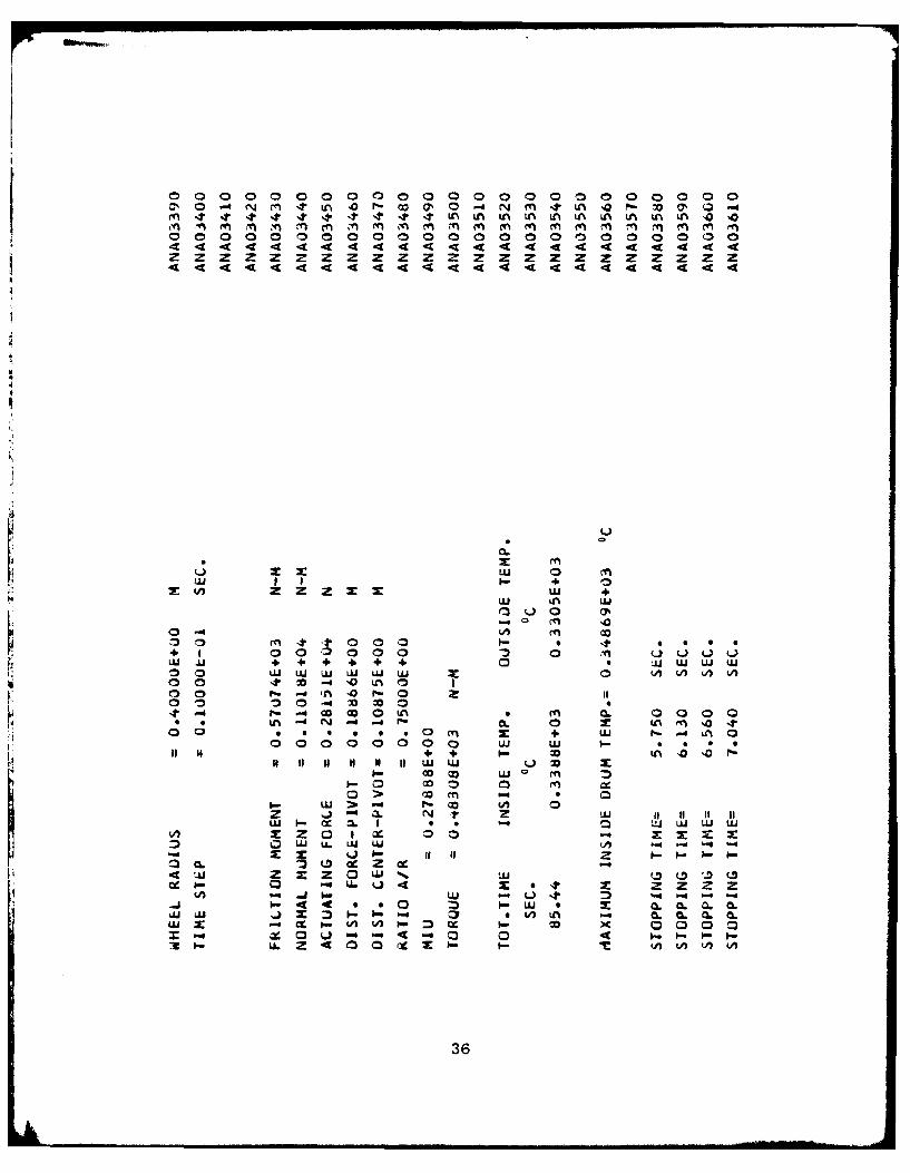
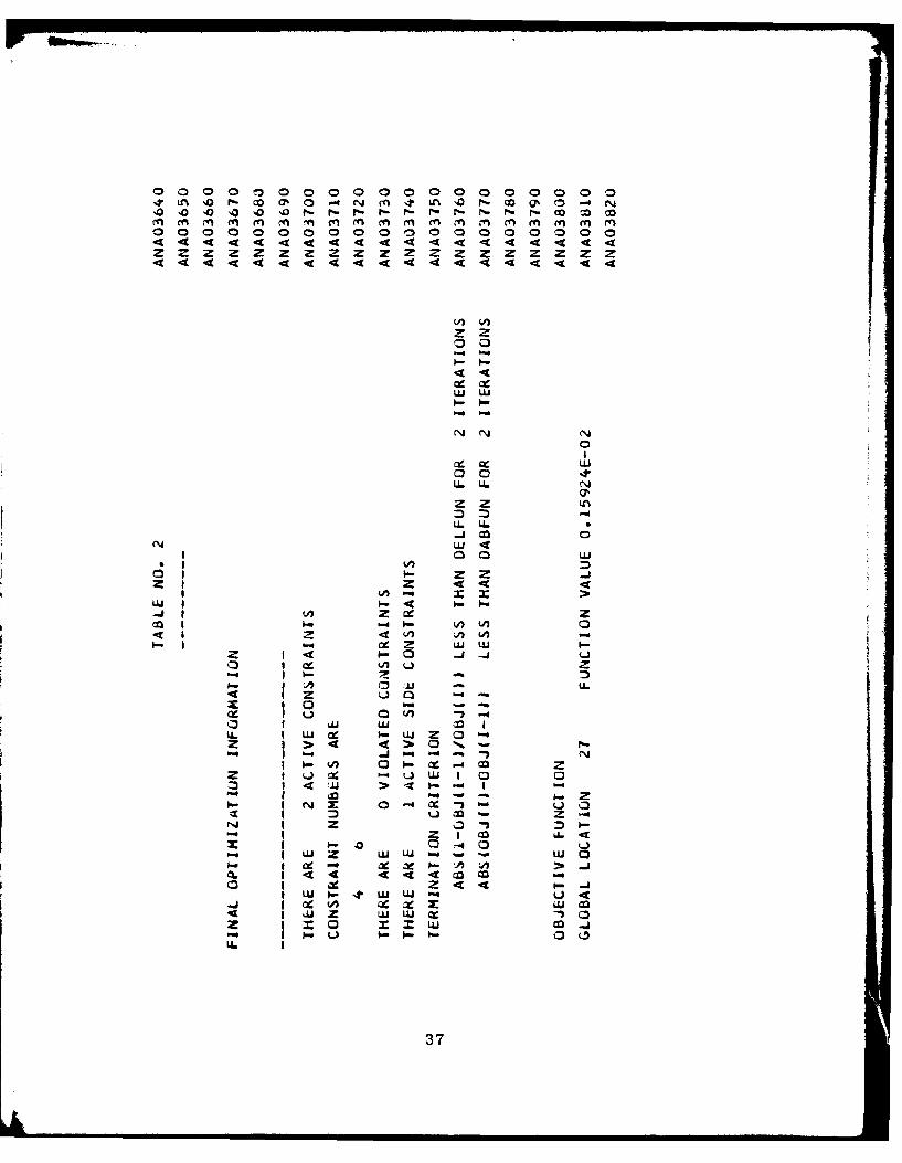
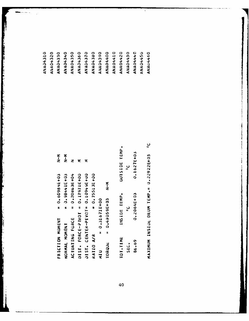
in Table I and Table 2.
28
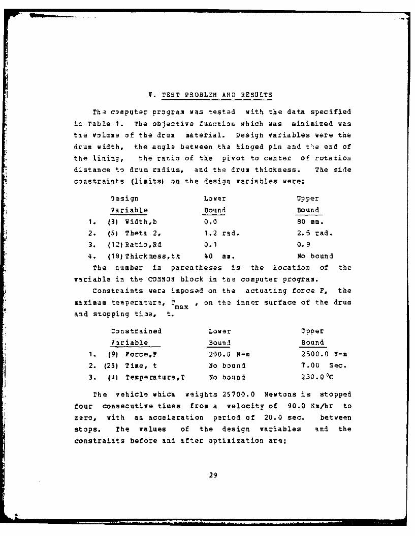
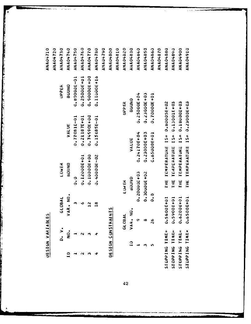
V. TEST PROBLEM ANiD RESULTS
The computer program was tested with the data specified
in Table 1. The objective function which was minimized was
tae voluze of the drua material. Design variables were the
drum width, the angle between the hinged pin and the end of
the lining, the ratio of the pivot to center of rotation
distance to drum radius, and the drum thickness. The side
constraints (limitsi on the design variables were;
Design Lower Upper
Variable Bound Bound
1. (3) width,b 0.0 80 mm.
2. (51 Theta 2, 1.2 rad. 2.5 rad.
3. (12)Ratio,Bd 0.1 0.9
4. (18) Thickness,tk 40 mm. No bound
The number in parentheses is the location of the
variable in the COM33N block in the computer program.
Constraints were imposed on the actuating force F, the
maximum temperature, T , on the inner surface of the drummax
and stopping time, t.
Constrained Lower Upper
Variable Bound Bound
1. (91 Force,F 200.0 N-m 2500.0 X-m
2. (251 Time, t No bound 7.00 Sec.
3. (31 Temperature,T No bound 230.0 0C
The vehicle which weights 25700.0 Newtons is stopped
four consecutive times from a velocity of 90.0 Km/hr to
zero, with an acceleration period of 20.0 sec. between
stops. The values of the design variables and the
constraints before and after optizization are;
29
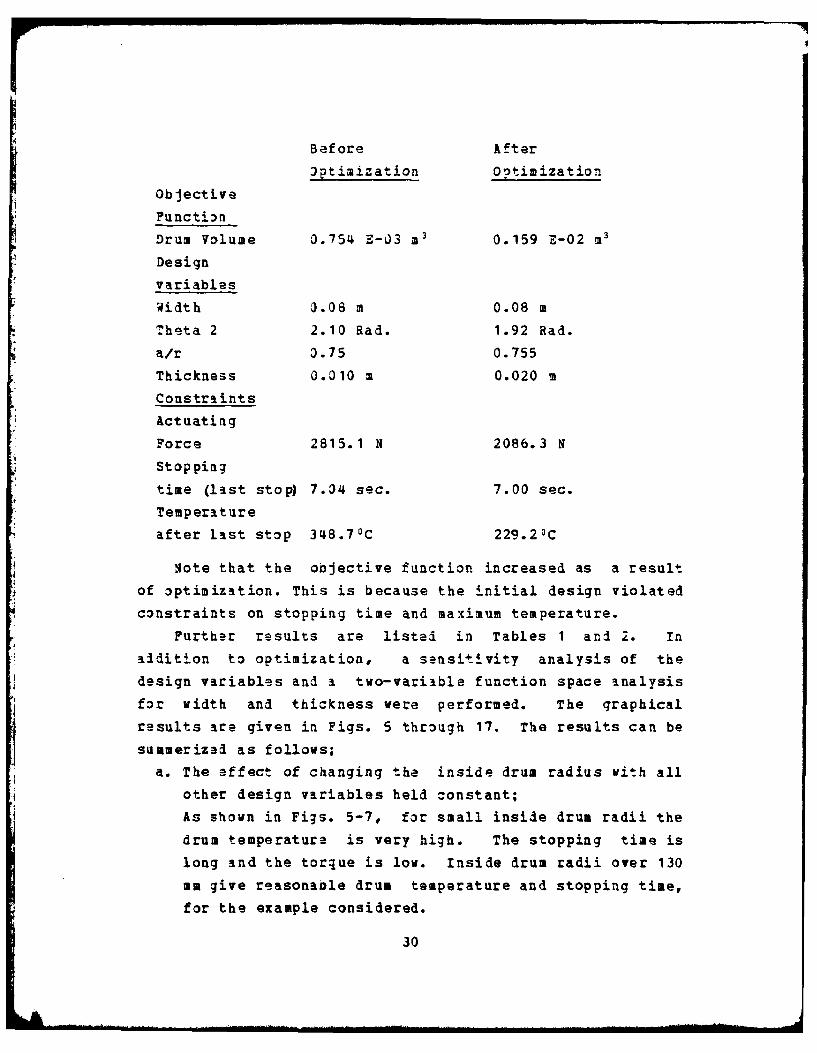
Before After
aptimization Ootimization
Objective
Function
Drum Volume 0.754 E-03 ml 0.159 E-02 ml
Design
variables
Width 0.08 m 0.08 m
Theta 2 2.10 Rad. 1.92 Rad.
a/r 0.75 0.755
Thickness 0.010 m 0.020 m
Constraints
Actuating
Force 2815.1 N 2086.3 N
Stopping
time (last stop) 7.04 sec. 7.00 sec.
Temperature
after list stop 348.7OC 229.2 0 C
Note that the objective function increased as a result
of optimization. This is because the initial design violated
constraints on stopping time and maximum temperature.
Further results are listed in Tables I and 2. In
addition to optimization, a sensitivity analysis of the
design variables and a two-variable function space analysis
for width and thickness were performed. The graphical
results ire given in Figs. 5 through 17. The results can be
summerizad as follows;
a. The effect of changing the inside drum radius with all
other design variables held zonstant;
As shown in Figs. 5-7, for small inside drum radii the
drum temperature is very high. The stopping time is
long and the torque is low. Inside drum radii over 130
mm give reasonaDle drum temperature and stopping time,
for the example considered.
30

b. As seen in Figs. 8-10, the affect of changing the drum
width with all other design variables held constant is
the same as described above.
c. The effect of changing the drum thickness with all
other parameters held constant is; For a drum thickness
up to 6 am, the stopping time and drum temperature are
consilerably high. Over 16 zm thickness, the stopping
time e ains almost constant. For a small thickness thetorlue is very low due to the high temperatures. For
thicknesses over 20 mm, the torque remains about
constant.
d. The effect of changing the angle between the hinged pin
and the end of the lining is; For a small e2 angle the
stopoing time is 7ery long because the torque is low.
The stopping time becomes reasonable when 6 2 >1.8 Rad.
2bvi:usly there is an increasa in the drum temperature
as e2 increases but the ovecall change in temperature
is small.
a. From the two variable function space, Fig. 17, it can
be seen that the constant volume line and the constant
temperature line are almost parallel, this leads to the
conclusion that for the cycle taken, the drum is a heat
sink, and the amount of heat dissipatel by convection
during this cycle is small.
31

1I
VI. TEMPERATORS aAISE - SIZMPLIFIED CALCULATIOV
A simplified way of finding the temperature rise of the
drum is by using the equation;Q = WcAT (40)
and setting Q equal to the amount of heat generated using
Eguation (21) from section II-D-4. This equation is in
common use in engineering texts (See, for example, Refs. 2
and 8). The temperature rise calculated this way, is the
average temperature of the drum, and not the temperature on
the interface, which can be much higher (depending on the
rate of heat generated). Extreme temperature gradients cause
distortion and excessive surface wear. Therefore it isn't
always acceptable to use the simplified formula. From
experience, it has been found that the surface wear
increases dramatically as inerface temperatures approachL430 to 5) OF (205 to 260 °C), [Ref. 8].
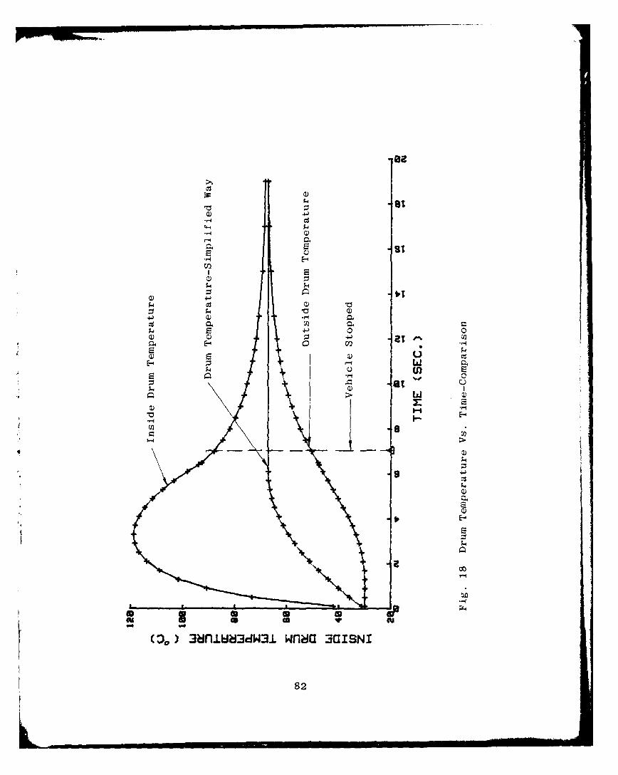
A comparison of the temperatures calculated on the inner
drum surface, outer drum surface, and the average drum
temperature calculated, using equation (40), is given in
Fig. 19. The graph shows the temperature rise for a vehicle
stopped from a velocity of 90 km/hr. From this graph, it can
be seen that the drum temperature, based on equation (40),
after the vehicle stopped is about the average temperature
of the inner and outer surface temperatures.
The results show that the drum will reach an uniform
temperature of about 58 0 C, in 15 sec, after the vehicle has
stopped.
Calculating the temperature with the simplified formula,
can lead to errors in the time needed to stop the vehicle.
Because the temperature calculated with the simplified
32
formula is lower than the temperature at the friction
interface, the calculated friction coefficient is higher
than the actual friction coefficient. Therefore the
calculatel stopping time will be shorter than the real
stopping time. All this is true , provided the friction
material behaves as assumed in seztion I-D-4.
Because high temperature is detrimental to both the
stopping ability and the wear characteristics of the brake,
it is important that the interface temperature be calculated
with reasonable accuracy in design. Fig. 18 clearly shows
the temperature differences resulting from the two
approaches.
This difference in results is compounded when the
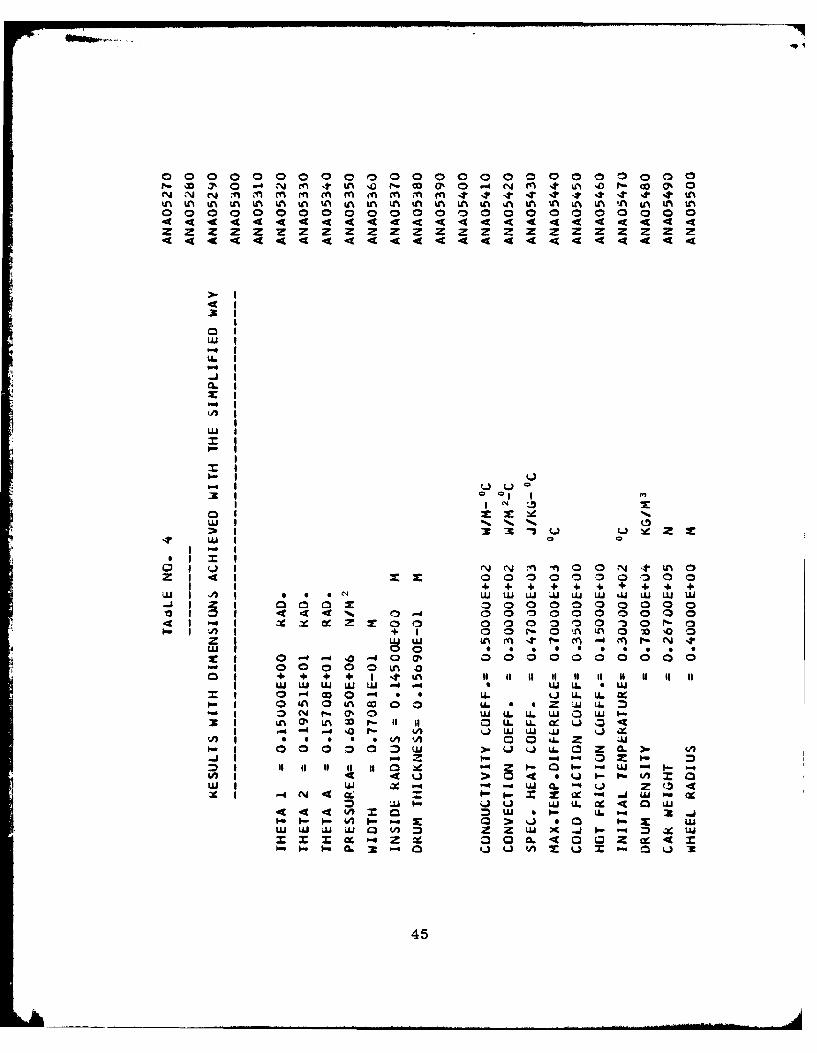
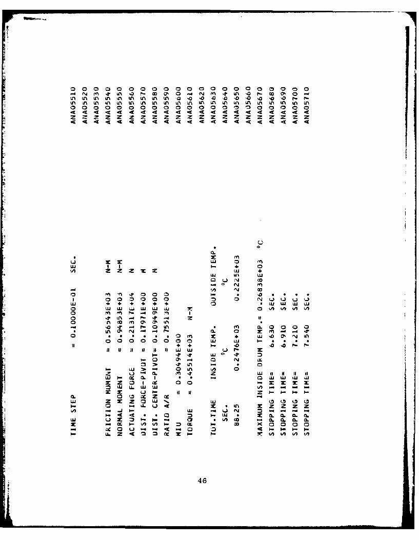
simplified equation is used for design. Table 3 presents the
design results based on the simplified approach. This design
represents an apparent material savings of 27%. However,
when this optimum is analysed using the finite difference
heat transfer solution, the maximum temperature is 268.8 0 C
and the last stopping time is 7.54 sec. This time violates
the constraint by 7.7%. Perhaps more importantly, the
temperature at the interface of about 269 0C would surely
lead to premature failure. Therefore this design is clearly
*. too unconservative to be acceptable.
33
VII. CONCLUSION
In summary, a numerical optimization program is an
effective way of finding a solution to an engineering
problem, provided reasonable care is used in formulating the
problem.
VIII. RECOMMENDATIONS FOR FUTURE INVESTIGATIOUS
The study has shown the feasibility of using numerical
3ptiaization in the design of Internal-Expanding Rim Brakes
with two leading shoes. Further studies on the same design
may be pursued by eliminating some of the restrictions. For
example;
1. To add heat dissipation by radiation.2. To investigate drum temperatures for a drum with fins.
3. To take into consideration changes in the surface
pressure as a function of friction coefficient.
4. To r-peat all the calculations for a drum in which
there is one trailing shoe and one leading shoe.
5. To add the effect of centrifugal forces for clutches.
34

000~~ a 0 aOOO OO OO 0ONC~ In 't 4O~ 0 .- A '0 r- Q 7J Q 0 - N m~ -- LA 0 tP- .50
z z ~ J NN NN z z z tz z m z
m 00 a I
I :D (Jm 1% n i 0
a 0 0 n
+I +I t 01 f If 1 1 0 f i
4 w 000000000. c0 0 *n LULU Z UJ L 6 LU D L
44 r-% W6600000000W
W LU wA U. !- c z 0.~*~Z~ ~ :r--O O 0 0 0 0
I. 44 + I ' 0 >I N I I if II (A XI-U CC LUJ 0. P" _ULL .7 ".D .
4. 004 0M :D U UJ U.00cc ~ 0 wa 6L. Q. 0 a U
N mO 'A xJ WU X o
0~ Z wZ -
I I if I I 9 0
W I 4 35
0 000 0 0 0 000000a0 0 0e1)0000 00 0
4x44 444 444444 L
ri (0
0 0 -4 f% LU 0
0 LU LU LU LU 00 LU00 A-. 4. 00 c n0
I.- -44f a!x I r 08~~~ C0@-. : e . L
0 aA '0 '0 (; o o!J '
01 If + + 1- 00 0If o I I 1 1 LU uj Z X:
L - t . I 00 0 L LU LU LUP- 0 co 00 0 -c
0LU I- ( U.1 LU LU 'A-4 U
I f It z l'- 16- 6-CL 0 e z
w z a Lj 1%LU ( 36
4 Ln Q~ P- w 0% 0 -* N m 't in 'o r- w Q% 0 N4~%
zz z zz z z 2z 7zz z z zz zz z
vI) A)
w z
CNN
L6 LL N
0%z w4
0I.- z z44 4c
ca .4 V) (A 0149 4 cm A (A
b- ae z ZL
9'--
I zzIL. 9 L" LU ZLL I L- cc -J -Z N
I-I-- cc -O
z a - -
I 1 40 M- 0L-4 IU Z w W -~W 0
00 x x >
4 9 JZ LU Wicc 1(Zu CO -j~Z
37

0 00 00000 0 0 0 0 0 00 n0
IA . - co (% 0- N m 'r Ln 1O 1- 0 C" 0- N (n It LA
0000m0 0 P000 ,000 0 %0 00 0 00m4 4 4 4 4 4 4 4 4 4
~~~ Oww
Q.L 000
-4 NC of00
_j~~W 000 .
C. 01 00C)~ 0 0
S-4 0 C1 ) % 0
S 0 (J I 0 N. N I-+ + I U
C3 N0 N 0 NO
0Dr-00 N0
Ico m U 10 N 0 (
0 0004'00
0000 Z LU U
-N I.- 01 14 x x
UIa i
LI4
38

0 00000000 0 0 0 0 00 0 000~ ~0 - rN rl Xt -0 r- m~ 07 C -4 N In 4 6n o r- 0000 - '-4 -4- 6 .4 -- 4 -4 N N N NV N N (% N~ N
LA
0+ +
* ~LU LU t LU LU W u 'U UJ LU U.) L LUJ
4 44S X 0 0000 00In0 000
cc~ ac 0x 0 00 00 (5n0e* 00+ I 0 Po - 1!3 - LAO0 m -0 00LU Wj L m .r'- m19 en r- cm N r 4 4
OOOOOLA co+.~ 4 4 I It a% If 11 1 11 11 11 H1 1 It 11 II
LUi LU U LU LU -4 14 LU U. i Lu0-4 co0 0 0 0 QI. (..). LI z0 LA 0 nA 1'- 0 0 LL 0 *Z Lu U. :3N r- 0' 0 LU LL LL LU OW i
L % U, 40 H 11 I 0 U.L u. cc 0 4.- 0 Q ~ ~ lLJ W L Ll. z 'U
z " -0 0 LA. L
44ci : <U I->wLa 4 0 .J1 4.CA
I-- (n f w - le Q > wXU.; L
X-I I-I I- Z >LJ Q *.4 0 9- Z LU: LU
39
-I Cf S L( ' f~ ~ 0 -4 0 ~ 0~ .0m It .dA- 10 1 z (% -t 0 't
0 0 0 0 0 0 0 0 04444444a444444444 0 0
z zz zz z zzz z zz zz z
LU P-0
I~1 IN-
0 a.
aU LU LU LU LW I-
C% rt Ln 00 04 c
> 10 0 -4 0I- LU > - 7 (A 0
LJ 1- (1 M. I 0 -0X Z -: c1 00x LUL LU 11
ZXZOW%,, LU0 i. 4% x 0%
LJ~ 0 I-Ic LU '- t~- C4l V) I- )- L) co
0 49U. Z 4 0c I
40

t L00 00 0 1% 0000 00000It tn m Ln LA InU A A inz '0 10 10 .0 4O '0 %0 Q
0
4L.
LL.-
'0a I z -
aI 4 c A L"
01cr wf Ln- 2-
-J ,L -U pL - 0U c -
w i w U..14 Ij > Z .J t
W~ Z W Z~z m
0 W " 4 >
Cf. - ) ui 00
44
r- -000 *-1- -0%000wc0w0 00 0m00w0 0
-4 -40 O
xn(I 0 Ln WLU 0
LU~0000
=. 0 0 -4 r-f C-L-j c U 0% co 00
0 0 % A) ~UJ
rl-~Q ?0 0 1-4Lu.J . V t
0 0~0 U 4
+ 44 1 0 0 C3 QL LU LU LU LUi w w w N
3I - 0 0 IA CL m
M000
c 0 m 4U '40 N w -0 ' N .f .-4 wU w.4 w ws fli cc 0 0 0 LU LaU-
> r- 00 3% NU L LU>j -4 0n if %0 c 4
0i Nn N N% c 0 a 0 0
I L Ja 00 0 00.0
4~~~~- -. WNO 00 I- I
*U * uj ULU L U L
000 AO 00 (A
420 0
.~~ o '- C 0 0 0 0 n 0t ' 0 0 -0'0'<'0%0'<%<000<00000
M-
00
0 .4 0I
0 0 in0
+ ~ ~ ~ ~ 4 + +. .4 4 + 4.4.I 1 f I 1 f I t if I 1 1w 0 w w' W LU0 Lii LL LU LU L U L ..
0 44 L. 0 U. 0 0 0 0 0 0 0 0kn m 00 0 L.00 00 00zwL
Ln 4 Ul 0 4.i If 0n U.- LL, lty 0 00
00 P r- V) 0 w 0 0z
LU vi LU L U -0 Ll . z LU
0" z Io0 0 - aI x. U.D
o 4c4 0' 00 LU U.0.U U
uU -0 ki w' I U. x LI 0
m =) LU 8. L. X
1, UJ- aIL > uU. x LU '.4 U ' Z wL I X .
x C9~ - Z -4 0 C L 4 -1 x U
43

L o r- oo 7% 0 (1) -t~- 4 - P N N N N N
Ln f4A i lAl I LN in M tin In
0 0
00
:z 44444 0'. LU J. wU LU L
'It It4
. * * .0 4
44 44
0 ' 0 -4 In 10 t A~ r- (D 0a% o o~ ND r- . n
tn LN In In In LA LA tn 1%In LA LN LA LIn n 4~A iAIn A in LA L %
)i I
4,C3,
LU L
U.1I
4U w IlI l l
-. 1
LI,
V) Il w 0 4
V)141 aaU.I
U.1 U. 3(j z (x WI "0 0
CA =I IA .:
X9 19 aI
01 QI N ~ ~00 N4 LA
-4 N m -. tn QO I- w ON 0 -4 N m -t LA '0 t.- m ON% nLA L L tA ALA LA '0 00 o 'o 'o O o 'o o--
tn .A In tn Ln in A UNL Ln LA L LA m A Ln ui Ln LA L L t tA LA0 0000 0 a000 00 0 00015D000 00a0
~U.
0 0U
LU Ul LU
N c
I a 00 ~0 C 0N0 ~ ~ ' r-L L U L 0 LA A L A0 'LA I'dP 4 t-I
0 10 Cl N' 0'
0 0 0 00 0 LU LU 1-- 0 0 o * 1+I 4 + 1- 0 10 0 r-
it 11 If if if 11 LU WL j rI-. 4LU 0 '
I- LU> 0o LA LA 0
LU U -. 4 0. LUUS J I- LU m. 1I 0 w~ w -
z 44 * w0 I-- x-L x x xwU LI L w w 0n -aoa "" :
Z ~ x~ z- La~f W~ -A004 .9I 4- 4 0 0)m f-L A L M (
U.1 '& 40X 1-00 -- Q L m
46
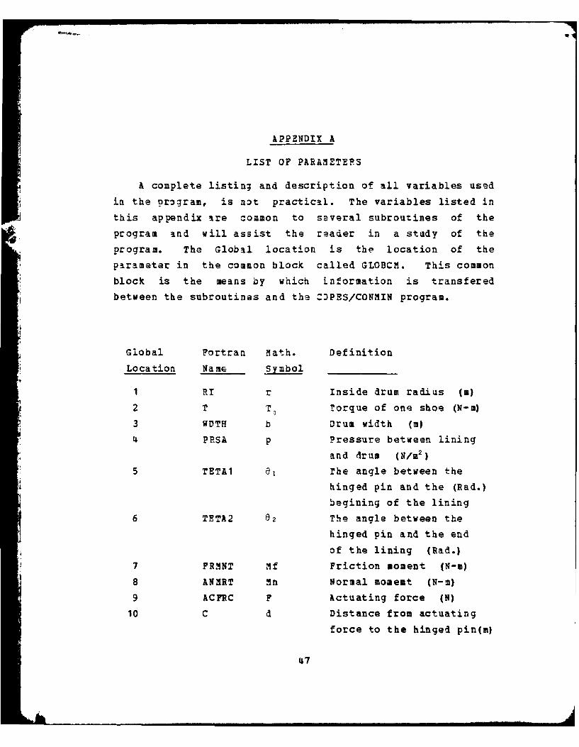
APPENDIX A
LIST OF PARAMETERS
A complete listing and description of all variables used
ia the program, is not practical. The variables listed in
this appendix are common to several subroutines of the
program and will assist the reader in a study of the
program. The Global location is the location of the
parameter in the common block called GLOBCM. This common
block is the means by which information is transfered
between the subroutines and the C)PES/CONMIN program.
Global Fortran Math. Definition
Location Name Symbol
1 RI r Inside drum radius (m)
2 T T o Torque of one shoe (N-m)
3 WDTH b Drum width (m)
4 PRSA p Pressure between lining
and drum (N/I3 2 )
5 TETAI e, The angle between the
hinged pin and the (Rad.)
begining of the lining
6 TETA2 e2 The angle between the
hinged pin and the end
of the lining (Rad.)
7 FRMNT Mf Friction moment (N-m)
8 ANMRT kn Normal moment (N-2)
9 ACFRC F Actuating force (N)
10 C d Distance from actuating
force to the hinged pin(m)
47

11 Q Heat generated (J/sec.)
12 RD a Distance from pivot to
center of rotation (m)
13 C!IU Cold friction coefficient
14 HNIU Hot friction coefficient
15 TMIU Friction coefficient at
any temperature
16 SRFC Drum surface area (m2)17 RO Outside drum radius (a)
18 THK tk Drum thickness (m)
19 DX An incremental thickness
(m)
20 RIIER R Wheel radius (m)
21 W W Car's weight (N)
22 DCCE dc Deceleration (M/sec.2 )
23 TOT Total time (sec.)
24 ECEN a Ecentricity (a)
25 NWRT Write statement control
26 TIME t rime (sec.)
27 VOL Vo Drum volume (m3)
28-32 TEPL(5) T Temperature at time p 1
(sec.)
33 NWR Write statement control
34 NWRA Write statement control
35 NWRQ Write statement control
36 NEL Number of elements
37 3SEG Number of segments
38 ?1 T Constant
39 G g Gravitational constant
40 K k Thermal conductivity
(J/m2c)
41 HCNV h Convection heat coeff.
(W/m2 -c).
42 SPHT c Specific heat (J/Kg-C)
48

43 aHO P Density (Kg./M )
14 DTAU Time increment (sec.)
45 DFTM T ilax. temp. difference(3 C)
46-50 TEMP T Temp. at time p (sec.)
51-57 RES Heat resistance (OC/J)58-63 TC C Heat capacity (J/ 0 C)
64 BIO Bi Biot moduli
65 FUR Fo Fourier moduli
66-72 NVT Control parameter
73-79 VT Control parameter
80 NELO Number of elements+1
81 NELT Number of elements+282 TETAA e The angle at which the
apressure between the
lining and drum is
maximum. (Rad.)
83 ACOF Constant
84 TII T Initial temperature(3 C)
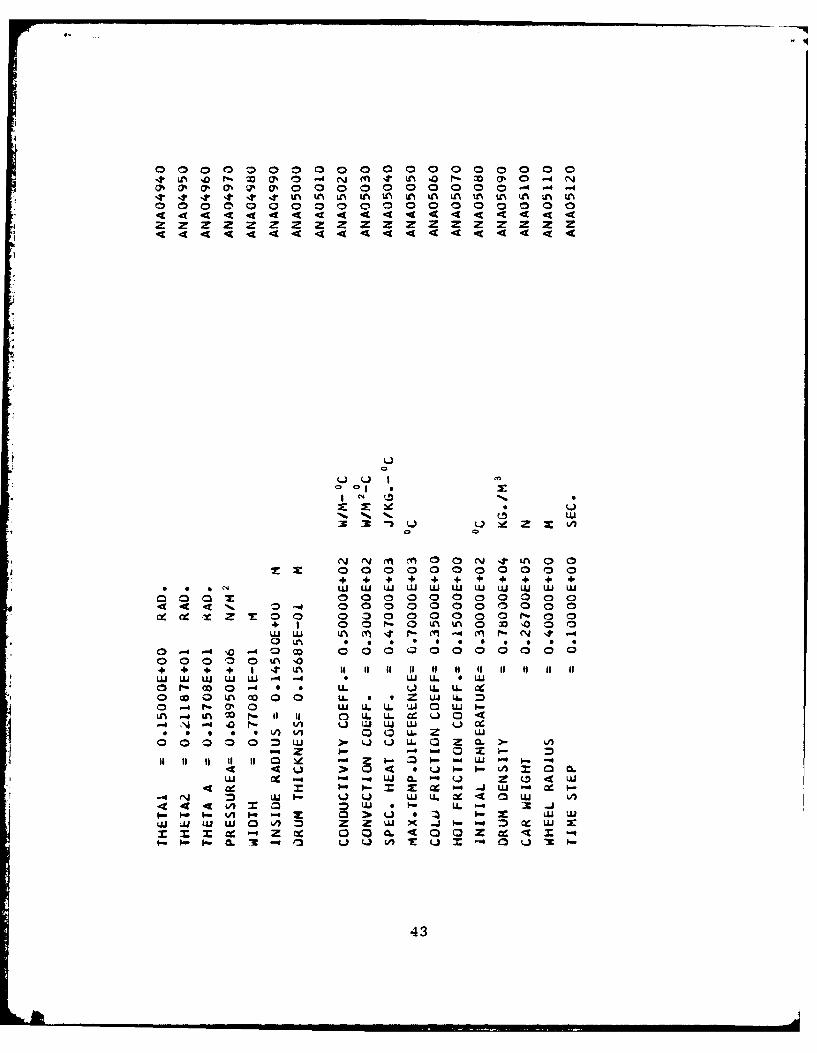
85 ZMAN t Time increment (sec.)
86 NSHU Number of shoes
49

APPENDIX B
INSTRUCTIONS FOR PROBLEM DATA PREPARATION
Although the procedure is straight forward, preparation
of input data for te program requires attention. Errors are
easy to make and difficult to locate. Input data is
described here for the brake analysis. For instructions on
data preparation for optimization see Ref. 7. Input data
should, in general, follow the steps outlined below. The use
of the standard FORTRAN Eighty Columm Coding Sheet is
recommended. Intege. constants aust be right justified in
the appropriate field. There are eight input cards, read by
subroutine INPUT, to describe th? initial design, material
properties and constants. Card format is given in
parenthesis followei by specific instructions where
n-cessary.
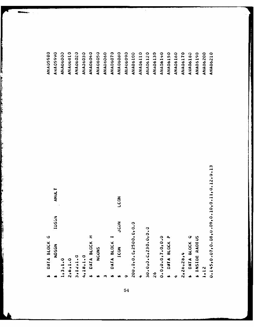
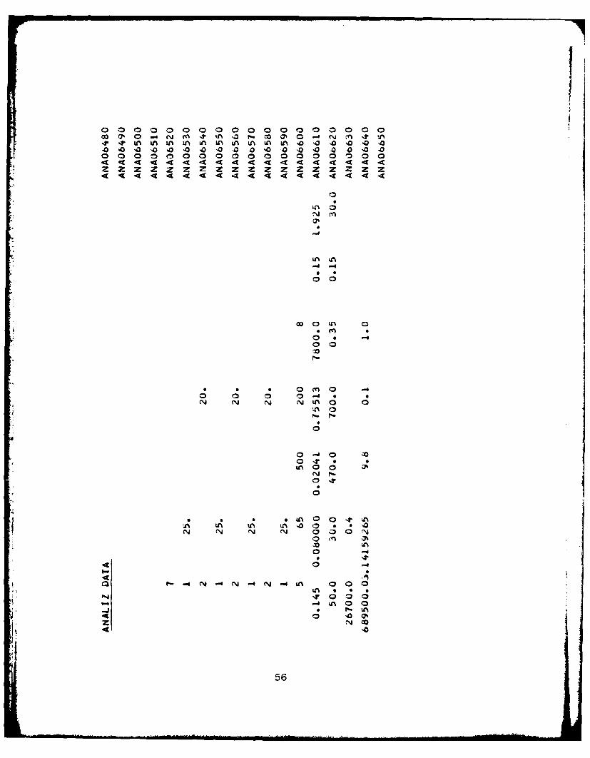
1. First Card (I10) - Duty cycle information.
Cols 1-10 : Total number of consecutives stopsand accelerations (NSEG)
2. Second Card (I10,3F10.01 - Duty cycle information.
a. Cols 1-10 : Control number.
1 means-deceleration,
2 means-brake not in use,
b. Cols 11-20 : Velocity at start of deceleration.
c. Cols 21-30 : The velocity at the end of the
deceleration.
A. Cols 31-40 : The time the trake is not in use.
3. Third Card (5110) - Thermal analysis information.
a. Cols 1-10 : Number of nodes (NEL).
b. Cols 11-23 : An integer number that controls the
amount of printout when detailed
output is required during the
vehicle deceleration. The amount of
50
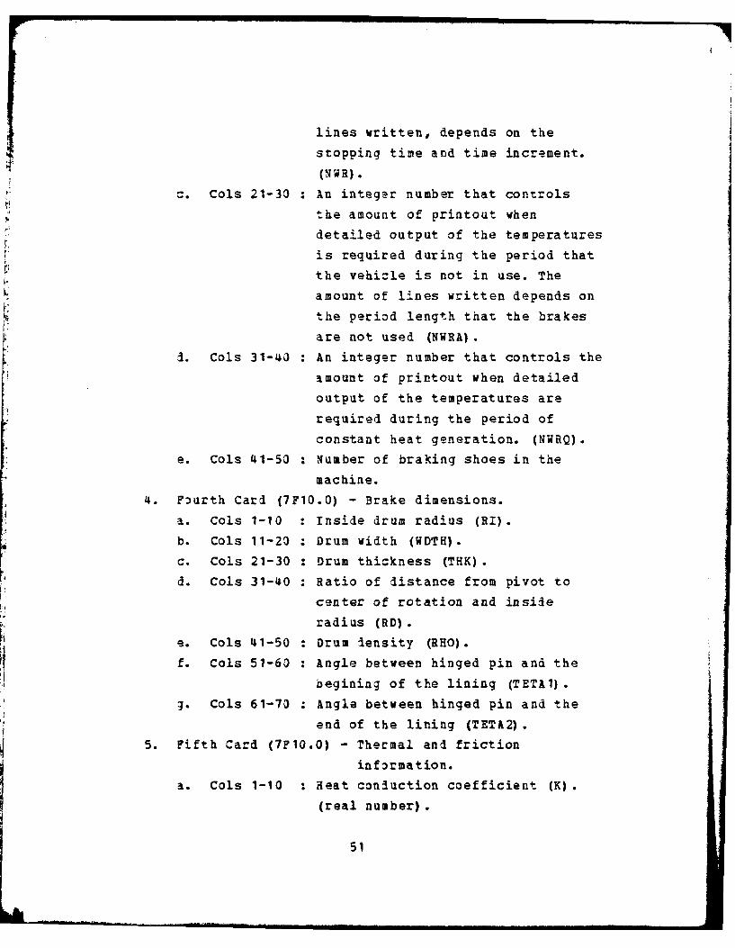
lines written, depends on the
stopping time and time increment.
(NWR).
a. Cols 21-30 : An integer number that controls
the amount of printout when
detailed output of the temperatures
is required during the period that
the vehicle is not in use. TheL amount of lines written depends on
the period length that the brakes
are not used (NWRA).
1. Cols 31-40 : An integer number that controls the
amount of printout when detailed
output of the temperatures are
required during the period of
constant heat generation. (NWRQ).
e. Cols 41-50 : Number of braking shoes in the
machine.
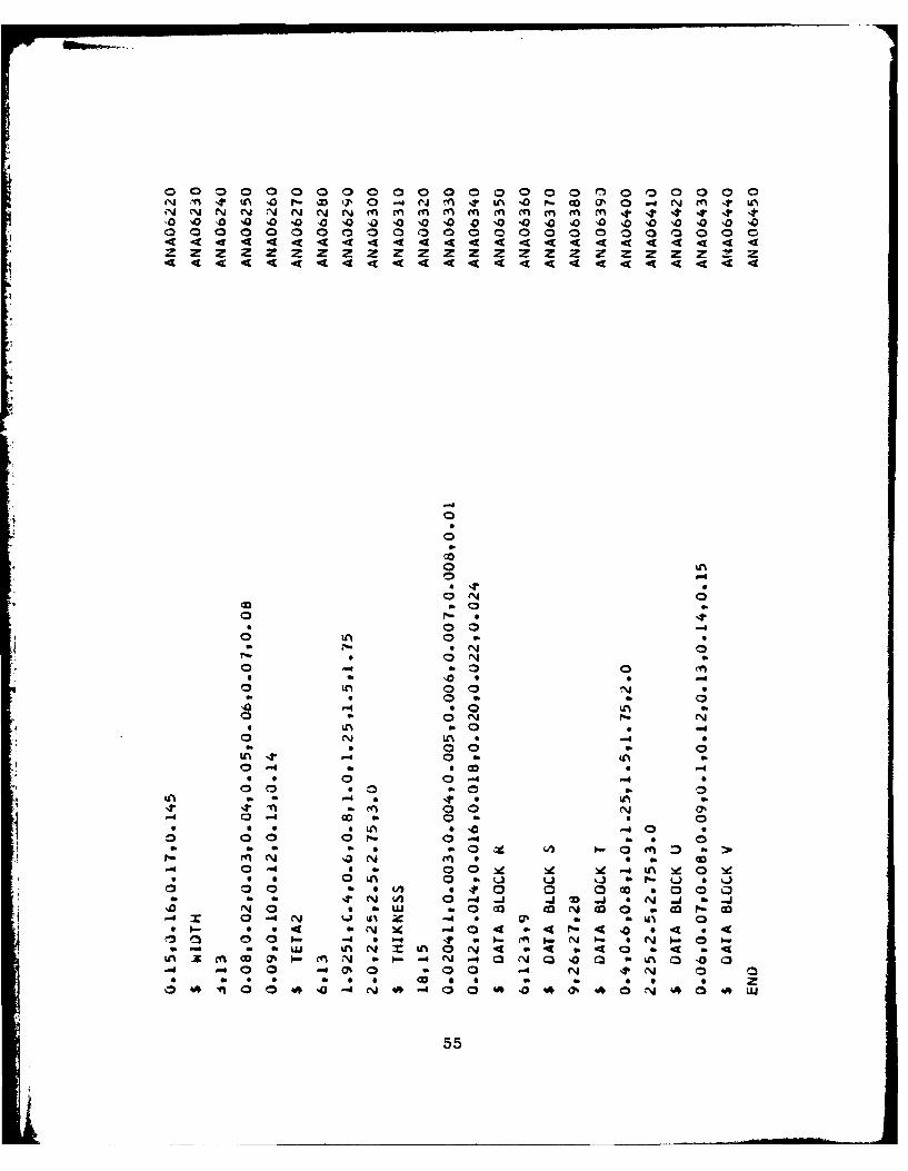
4. Fourth Card (7F10.0) - Brake dimensions.
a. Cols 1-10 : Inside drum radius (RI).
b. Cols 11-20 : Drum width (WDTH).
c. Cols 21-30 : Drum thickness (THK).
d. Cols 31-40 : Ratio of distance from pivot tocenter of rotation and insideradius (RD).
e. Cols 41-50 : Drum density (RHO).
f. Cols 51-60 : Angle between hinged pin and the
begining of the lining (TETAl).
g. Cols 61-70 : Angle between hinged pin and the
end of the lining (TETA2).
5. Fifth Card (7F10.0) - Thermal and friction
information.
a. Cols 1-10 : Heat conduction coefficient (K).
(real number).
51

b. Cols 11-20 : Heat convection coefficient (HCNV).
c. Cols 21-30 : Specific heat of the drum (SPHT).
d. Cols 31-40 : lax. temperature difference between
cold friction coefficient and hot
friction coefficient (DFTM).
e. Cols 41-50 : Cold friction coefficient (CMIV).
f. Cols 51-60 : Hot friction coefficient (HMIV).
g. Cols 61-70 : Initial temperature (TINI).
6. Sixth Card (2F10.0) - Machine information.
1. Cols 1-10 : Vehicles weiaht (W).
b. Cols 11-20 : Wheel ralius (RTIER).
7. Seventh Card (5F10.0) - Analysis constants.
a. Cols 1-10 : maximum pressure between lining
and drum (PRSA).
b. Cols 11-20 : Constant 3.1415927
c. Cols 21-30 : Gravitational constant (G).d. Cols 31-40 : Increment of time (ZMAN).
a. Cols 41-50 : The angle of maximum pressure(TETAA).
8. Eight Card (110.0) - Print control.
Cols 1-10 : An integer number can be zero or 1.
If zero (or a blank card) - only
the final results are printed.
If 1- the temperature at time
increments are printed.
52

-t Ln 'o r~- co 0 -4 C4 'nl 'r U-% I- CO 3 0 .- N C4 't LA 0 r.-AM LA nA UN Ln LA tA LA LA LA LA LA LA LA LA LA tA LA LA LA LA LA UN LA
zzZzzzz z z z zzz z z zz zz z z z z
44 4 4 4 4 44 4 4 4 4 4
Q Cc zx (Az ce C
I- a
zM
cm LU 0
a 0 04
CL 0 Z j c
44L
44
-5
00000 0 rCA00r '0 07%0 000000 1-00000Ln LA C\0 cfl' Q 10 0 10 0 1 0 4 C'Q 10 a 4 .4 0 1 10 4Lfla'0 '0 a0 04 0 C)0 '0 ' 0'0. '0444 '0 '04
< < At 4 4 44 4< 4 <4% < < 4 % -i -1 < < 4 < 4 -4 4cT z zz zz z z zzz zz zz z zz z z z
44 44 44 44 44 44ON44
.7
* c1o
(L Cr V) -c
0 0 -4 .
(I 4 04 0%00
*1 54
in. Q 4 A . r- W~ 1% 0 - 14 fn 't in 0 P. OS) 0' -4 N (4 -r Ln
-0 '0 0 -0 '0 %0 o0 0 a0 0 '0 0 0 '0 0 '0 '0 '0 '0 0 10 10 %a -4
4 < <At 4444 4 44 4 4444 <4 4 44<4 4d
000
10
N --
8 0n04 0
0 o 0 cc0*U m' N 0 r- o
N zN ON
O 1 49 0 0
0n N m LC% '-A
00- -4 0 0 in W 0 a
LA . -. 4 . 4 S55
It 0 kn Ln Ln L n Ln W Ln Ln~ '0 0 10 '0 '0,0 10 10 10 .0 10 '0 '0 -0 40 10 40 10 '0 0 40 -0 4
C
0 -t 0
0 It -00
I-n
6~1 (T.0 ~N~~~ N LoA
01
56~
*.. Adi -
ZZZZZZZZZZZZZZZZZZZZZZI4444444444444444ZZZ ZZZ ZZZOzZ ZZIZZZ ZZ1444444444444-k. 444 4 44 4 44 4
Cm .:-' .
Z- 4?I
z 04 -e
1l I- vAIoU-4 O~
= NU O-Z ft c-ON.DZ 0'W -4z O* C.-
0" V) .Wu jd .4mNC
- NJ 4- Pi- 1SC
- .JLU e-- . LLJ4 .
LU x .4 5 -cS *.W >0C. d4 W L0. cc x .ZxLI7. LI
CL LA 0.... .4
ujg 0It -j e -J-JI.-- < ^
z NJO-A i.. 'JcD L
Win 041'4 cv)4 * JOUJ - t57 - Q-
4"
00000000000000000000000000
2ZZZZZZZZZZZZZZZZ
I--4e4u4 44
o- -Z w
l- -u -. 6-
Ln~J am-4J
(A .X.14.W.M.-O .
e-XCLI0 - 4-.
t4 -0 LJ -4 .Z-Z0X3LU i 0-I.-
1- .4-XAz )~ -fol.Z
JO -Z .,- w
0. 0l-c(0 *I- 1- 0d--co tn.GAL CY> Zf-j 0
a fO: - - C X -
Z .b -Z
-t -.- 9w " 0:D .. X0.Z. W _j J
(LW X49La> LnO Zu- . 0-e~ -L
S-O .ZM .Wz- ~-wa. -40
I-U =Z .-. 4 - NM MM w .3)-.g-
'-a CIO:).x X 0
ul ..o.j~aCi 0 .0 000000 .- iLL-Z30O000090~ UO' L LLP-Sq
0 000-4 CI 1
58

OoOO00000000000000000000000000000000000000000000
cyo~ O~OO~%OO0OOOQ0O.-
W-x-
4: a2=0*
- .Z ' a
4 -01- .4-CNZUZZ4%0m2
OZf-I'-Z
... LUO.I--
i'- OkiJ a41-
Si) &nLL) a
oc WI-C -LUJ -W 0.0 ft0. 0I-(0.F-
xLU -(-n tA 0
LU 0U Sj-lZ - t
w -l---.jj 0l -4 .4 4)
v4*0 *U U.; 0J -0 *M %V~. Cd> Z wZ * * ftI
cc Lu .Ot:)1 oz M- .4)~ . -=' i oct +WU.7 o- )( " f4*( - 1
(A 0 I~ )0I 0* X0 + W4 ILL F-...&flE- - S -0A Wo- * LU .1> 0* 0 P>ii 0
W J m J-Nao 4 11 1 >- ZLL *N 04 1- LU"Z'-=Z +.. +S. -. o. M* < <. - -zN 11~ 1,
LU% ftU~ -10 z-.1-. .W- *1 LUO If MW If P.-W d It *CA'j * I2 -t i-.M-.i0ZZ 0 If 0.-. -Zj. I
- )(n2-xo-dzz -4Z 44 .42 0- ' -ZWW 4 a 1Zj) 1149oz rL 020g if OZw~ 11 It 0-P4d-gogg CA oo.-.-ozz CL CC--O"w I. o
Li11.W4I.. Z3-N '-Z2 W 11 CAZd)U U w .. 4.,.a -z 'w Doawwo-o-~ Xo~wcLWw~ UJou f-I.
.4 -4VJf4~ 44 49LULU l'-
59

zzzzzzzzzzzzzzzzzzzzzzzzzzzzzz- zz.zz6
O0 .0000000000000000000000
- L
+ -f
LU -z (m 0-
LOa
LUWO
+ % . - 1-
x I.-C.
Lu U. 00
aJ Z 0 --a ILII - -04M oi~
A -o
*U - M. 11- 0~ ~ LLU
MO-0 mI-- l -.-
0 09. I-LU 3 W O- * wmc (n 0.0c x Q4uzwMW-
LU-C Z~ 0 L Z-LJ 0 -g .. i-WNO W4- x aU a o 0 -4 o- --
I-* 00 cc n *% 0 -Z-.f -X ow.(.lU o x (.DI- ft3 .c: fwtOZ (21 L
*Wao-Z0 a- 00 :DD wooo4 V) *Q 1I- J0
tn- Z) 0 Z1 :D - y t--is -o d )4Q*LU *. Wa0%X 00 0 M Q- W -4 4
NI1MIAo a a. c3NrD Q z-z if .41j --z z> <1 Z
N~~I.~4c A W e --!D LULdV7 cc 0~J W
AaO.. ~ 0 0.Z WW.. - ..
WNAC~a4 * 4 4 4 0* LQQ -aN 04*i t.-40
A - LU 6 0 (~. - 4 I
OO00 04 04f- w mm m 0000000 00400
zzzzzzzzzzzzzzzzzzzzzzzzzzzzzzzzzzzzz
Lu LU LU wi
CL L 0 - (n .
Lu Lu LU Lu -v9 %
9- 0- 0 0-6 ~0. Z<
C5 a -00 0
aJ .j 00 ON0 _-- 7-Z a..a. a. a.
LU ) 4 LiU Luj ILU
1. $.0 *- tiz Z- SczP-P 00O I-LO C- I-sO sO LUOI.Xgcc 0i 0-' 0v 0c 0c4 A ~ M kn cL)
Q r 4 -- w w~ -> r-": c 0 0- - 0~ 0 9-3 O UX
La La *I aa -I Ou Lo OW4LA0 <ZO 0 0 0 0 00D41io19
:3 OOZ 0-0 3b 9- 1000Mz Z- 0 1-X z- Z "- if 1 *Xz O
-. 0 %lum W4 4 LU +*U-~ 11 4 *L *cL aC0- I- ~ i- SI-c.,ip I-I-. wo~wC.D
- 0 IJ -4 -0.a LoJ( -> O..-0% 4 S aSS S.~:
3 3 Z'.4Z (~ -t~l Zw-.4 3 ui~61l

O00M 000000000000-(mlto* O00
ZzZzzZZzzzzzzzZZz~zZzzzrz
-ur -Z.
LU e'Nzz- .*
>ZLUjOZ. 6.
LUJ Z< -=t-J* 43. 'J
LU ~ ~ LU -m
> -eccuwo.- -LU .JU.(J.) "P-s4
z wc,.0>c3o. I.4 -Ztz cc ..i
a4-3LJ4W 3 LuJLU -wL -= 04- U. Zcc 01,-cct -4* % -
4q <<4IOU:)1- LlUCC **C 4-U. I
LU -wL -* -* +. *
A.O..1-X -J- + M
I J<4wzg.I -4 " +4 =t -OML~.0 -X LU .- e-z ow . -..
LU -% w . .J-.0- x W~4- 00.w.W4I wu z
ZU LU a Q -. 4 +I.- U aUw.uCa>%w- -4 LU
-C 4XCc-ccoe -- I -
cic Qj -o0~n ZM- 0. cc4 i Un -. 444 -<
4 qccce. Lu LL'.3 Z.314Emm 0 4~* .
u.iSZQ -Zu.*W..j- 0 .jLU I--LUD= - - 7(3* N W..lz 1--cCO* *zcc I ZO.
LU J:X~zww * "M
11 1Z1Z -. u. j 11-11 -
CO ozorw ~~-.0-c0 OZ ccLUXL- wNC. Ix
4-4
62
,ooo-m -titm~O-co~
44444 44 4 4Z~zzzzzzzzzzzzzzzzzzZzZZZZzzZZZZZZzzzzzzZz~z
4t -LJ4 g
CA 4oO0AC
cc LU I- L4U Of 49ZLI- -. 0
Q- zZl0 Iic 1- z~ .4
ZX -=P-4 ifz -f( a"
.1 2 x -a..o-I - *
QLQV UUJ~-( 6 W0 0.1.1. 4 X
w- 44N >OW - I.--I-4 -. - -- U1 MI o40 N'1. U.1J
01-7390O.JW4 0W - I--
Wgq.4W 5-0-0%
:n1. .. JL .. 4 ftr OX4Lf.. *n LL1-4 ol_-1-ON 0% 0.W0 l- N4L1 U.
In -0 .2-Jt 0I-~' 1 - LU 4 4' ~ ~ - V- ~ ni. ~ -'4 U. N 4 .- I <~~ 4Z 0-'%Z 1.e 0 0*L 0 L4- -U J L
ccI- n JU.@ O." I (A W4W1 -00 - W sLU. ~ w w*Z1- *(Je I- I.- ~ .. Lx (.1*o - 1-
U.Z( -Jo -Z - - .... vW C.,* -QCCI- aW Q wU q Qz wL u .. JBt3 . I* *Z.3 d) -* N%- X I cc 0
- JL Zc3I7N> w 0 .f %'44I*01- 00 ~ I U. 2
0 I-CjC o-- :)cc*.n- clc-*c - LL. U.C) "-ft"2~ sZ>00* *.-. 0"W 0 -%-L I % jN z LuccQ -c: 0ZO aW-- (5-Z hI ~I4.il * 0. 1-I4 2 49 2:
4c d U-ad 0 wU 0 *:D* 0 4 u..0 ce I - - C4 LA I.-
Q <QXo -4u* U.-o 'u i. 0= L LU* Z l-L Iw CA a otXXC AL CAOriEO 4 4 LuQ-Lfl 0 uC* Z - (n4 UL
U. : NVLJO: - 0LI SQ s I e Q
I U. It (
ootJj.)J . CX - CJZ --) QL J C..I
63

.4zzzzzzzzzzzzzzzzzz
I- .U4 1Lz I L f
)OO00r0000000000000000000of04r U
I:k cL- UQWWO IIo- M-z L LU(AWu _j JO
14zzi-~L'QU G.N0j" XU<U yo -um -4 01 *zl.,L1:)L1 x
iac 0. U .)Z J
>ZUJOZ :of-%
Z-9 vx- 3 ie Z=X3 Ztn~Un w= 00000 =.-O.$ * On
!30,-Z - =-N - NN- -44.4 Cl)
-nxW0.b- cf m LO ox(-EZ ft*fl
QLL k..) C4 Am. 00 11'%% ~ f *gI-- O 04A. z4 -4 I, fl~u~notInNX-4
NC3J>0 "f U w o 0u 0 *. * * *&vrA a
0-304%= 1-Cf (~(%(JN
uIwL 0= ftl- :D ft 0 x SX aWwwLJLw -4 *%%0D-( cc 40r -Z 0 --4tnx a. .a -- N OUMLCCY 2.
"i b . .4~ 3 w ma. ".., na iti1it iit W-4 II cc x
LJJ-4 * 'J. ft =L. T.% JUn*%, . 0 O *%%LJ it )(-4 %.
0%- P- 'cOoO'. :) & C3N NNSI e- U.GJ= 1
g-- Lu (Jw~ wo IIQ _ M-N WO-w Af-xW-QI. x- - LWTWGWIo.Ntj.WW.1i
0 A W 1_j - .. 0 N oIIIju % Z L I.
- - W'Z OLU *L4 Ll .4 11 CCUN~~0 W 0 00 IJU .OIIUN
ce -'NZ3.L a a- 0 000 00
64.LI-L

APPENDIX E
W1 W 2
Clutch or Brake
Fig. 1 Dynamic Representation of a Brake or Clutch
65

p4
Direction of Rotation
A 62 Shoe
Lining
Rim
Fig. 2 Brake Assembly
66

Drum Thickness
AX
1 2 3 5
Heat Generated Convection BounderyCondition
Outer SurfaceInner Surface
Fig. 3 Finite Difference Model
67

COPES CONMIN
INPUT ANALIZ
OUTPUT
TEMPR TEMA
i,- -
BRAK
Fig. 4 Block Diagram of the Program
68
(z2
= E1-4
1-4
z
*1l
1 2 20 In -- a r)
N 0 cZtu cu cu c
(:))Od31 n~a3aINI XW
69V
U)
LIU)
z
tbb
cuj
(*03S) 3WI.L DNIddOIS
70
cr.
ix
C3
LLI 2
z
bD
(W-N) 3flowi
71

I
iT'
TO
68'
-4
2
II-
z2
2
-4ci,
-4
22-4
so'-f
bD-4f p us'3333 31S
31 -
72

.Iwo
.we
1r'4
-I-
bb
*:6.
04
U) U U) U VI
(003S) 3WID DNIddO.S
73

Nor
E--
74.
0J-%1
U)Li,p6 z
cz
C)
-4
'dW31wnma3alSI X2
75 29-

Le.
'S.
.mo
U 0
low 4 l
16 ~ ~ ~ 1 L ----AC33S)3WII!)N~~dO2
76)
Iw
*mF
91 " ,
((TS"i-. cW
.Is* 0 E-
(W-N) 3flowO
77

Sl
.4-I
8*1
raft'
(00) dW31wn~a alSN 'me
78s
ix
9.9-
902
.. 9-
(*03S) 3WIJ. DNIddOLS
79
EA
IxI
s8.1 1
m
0:
.4. 6
,. .0
(W-N) 3nomo.
o
Si
E-44
0a 0
00
0 PL4
*186 CO
0.
0W HIM
81 -
Cd)
-44 C)
-4
5.4 0.4
E. C)
5.4 C)
C) .;-4
ILL4
S -4-
4V 4 C)
Co. 3alNdW1wiaIlN
C 82
LIST OF REFERENCES
1. White, J. A., Bcake Dynamics, 1st Ed. Published by
Research Center Of Motor Vehizle, Research Of New
Hampshire Lee, New Hampshire, 1963.2. Shigley, E. J., Mechanical En.ineering Design,
3rd. Ed., McGraw-Hill, 1977.
3. Holma, J. P., Heat Transfer, 4th Ed., ScGraw-Hill 1976.
4. Vanderplaats, G. N., CONMIN- A Fortran Program For
Constrained Function Minimization, User's Manual,
NASA TMX-62282, August 1973.
5. Vanderplaats, G. N. and Moses Fred, Structural
Optimization By Methods Of Feasible Direction. J.
Computers and Stractures, Vol. 3, Pergamon Press, July
1973.
6. Fletcher, R. and Reeves, C. M., Function Minimization
By Conjugate Gradients, British Computer J., Vol.7,
No. 2, 1964.
7. Vanderplaats, G. N., COPES- A Fortran Control
Program For Engineering Synthesis. Course Notes, Engr.
Desiga Optimization, Naval Postgraduate School, Monterey
California, undated.
8. Ranks, J., A Study In Pneumatic Brake Selection. Horton
Manufacturing C3., Minneapolis, MN 55414, undated.
83
-II I! .. . .
BIBLIOGRAPHY
Baumaeister, A. B., Mark's Standard Handbook for
3ngineers, 8th. Ed., McGraw-Hill, 1978.
Dusinberre, G. I1., Heat-Transfer Calculations by
Finite Difference, International Textbook Company,
1961.
Hanks, J. and Dayan, L., Efficient Clutching and Braking
of High Input Energy Loads, ASHE Publication,
S0-C2/Det-97.
Hannah, J., Mechanics of Machines, 2nd. 31I.,,
Edward Arnold (Publisher) Ltd, 1972.
Limpert, R., The rhermal Performances of Automotive
Disk Brakes, SAS 750873, 1975.
INITIAL DISTRIBUTION LIST
1. Library, Code 0142 2
Naval Postgraduate School
Monterey,california 93940
2. Professsor G.N. Vanderplaats, Code 69Vn 3
Department of Mach. Engineering
Naval Postgraduate School
3onterey, California 93940
3. Professor David Salinas, Code 69Zc
Department of Mach. Engineering
Naval Postgraduate School
Monterey, California 93940
4. Defense and Armed Forces Attache
Embassy of Israel
3514 International Drive, N.W.
Washington, D.C. 20008
5. Major Mordechai ?eer 2
Military P.O.B. 2128
ISRAEL
6. Dr. Jim Bennet
Engineering Mechanics Dept.
G. 3. Research .ab
Warren Michigan 48090
7. Defense Technical Information Center 2
Cameron Station
Alexandria, Virginia 22314
85