No. 503

Trade liberalization and the evolution of

skill earnings differentials in Brazil

Gustavo Gonzaga Naércio Menezes Filho

Cristina Terra

TEXTO PARA DISCUSSÃO

DEPARTAMENTO DE ECONOMIA www.econ.puc-rio.br

DEPARTAMENTO DE ECONOMIA PUC-RIO

TEXTO PARA DISCUSSÃO No. 503

TRADE LIBERALIZATION AND THE EVOLUTION OF SKILL EARNINGS DIFFERENTIALS IN BRAZIL

(revised version)

GUSTAVO GONZAGA

NAÉRCIO MENEZES FILHO CRISTINA TERRA

MARÇO 2005

Trade Liberalization and the Evolution of SkillEarnings Di¤erentials in Brazil�

Gustavo GonzagaPUC-Rio

Naércio Menezes FilhoIBMEC and USP

Cristina Terray

EPGE/FGV

JEL classi�cation: F13, J31Keywords: Skill Earnings Di¤erentials, Trade Liberalization,

Tari¤s Pass-through, Stolper-Samuelson

March 15, 2005

Abstract

Skilled labor earnings di¤erentials decreased during the trade liberal-ization implemented in Brazil from 1988 to 1995. This paper investigatesthe role of trade liberalization in explaining these relative earnings move-ments. We perform several independent empirical exercises that checkthe traditional trade transmission mechanism, using disaggregated dataon tari¤s, prices, earnings, employment and skill intensity. We �nd that:i) employment shifted from skilled to unskilled intensive sectors, and eachsector increased its relative share of skilled labor; ii) relative prices fellin skill intensive sectors; iii) tari¤ changes across sectors were not relatedto skill intensities, but the pass-through from tari¤s to prices was largerin skill intensive sectors; iv) the decline in skilled earnings di¤erentialsmandated by the price variation predicted by trade was even larger thanthe observed one. The results are compatible with trade liberalizationaccounting for the observed relative earnings changes in Brazil. Theyalso highlight the importance of considering the e¤ects of di¤erentiatedpass-through from tari¤s to prices.

�The authors are grateful to Honório Kume for providing tari¤s data; Maurício MesquitaMoreira for help with price data; IBRE-FGV for providing domestic price data; Daron Ace-moglu, Jorge Arbache, Carlos Cinquetti, Jonathan Eaton, Marc Muendler, Raymond Robert-son, two anonymous referees, and participants at seminars in CEDEPLAR, EEA, EPGE-FGV,LACEA, Latin American Meeting of the Econometric Society, PUC-Rio, UNB, and USP foruseful comments and suggestions; and Andrea Curi and Rogério Mazali for able researchassistance. We thank CNPq for �nancial support. Terra is also sponsored by PRONEX.

yCorresponding author: EPGE-Fundação Getulio Vargas, Praia de Botafogo 190 sala 1108,Rio de Janeiro, RJ, 22250-900, phone: (5521) 2559-5844, fax: (5521) 2553-8821, e-mail:terra@fgv.br.

1

1 Introduction

From 1988 to 1995 the Brazilian economy underwent a massive trade liberal-

ization process. Non-tari¤ barriers were replaced by tari¤s, and tari¤s were

reduced from an average of 42.6% in 1988 to 13.4% in 1995. Neoclassical trade

theory, based on factor endowments di¤erences, has very clear predictions on

how relative factor prices should change in response to trade liberalization. Over

the same period, a decrease in earnings inequality was observed in Brazil: more

educated workers�average earnings declined 15.5% in relation to that of less edu-

cated workers. This paper investigates the role of trade liberalization on relative

earnings movements in Brazil, through a Heckscher-Ohlin-style mechanism.

Brazil is particularly well suited for studying the e¤ects of trade on earnings

inequality. First, Brazil moved from being a very protected economy to an open

one in a relatively short period of time. Second, earnings inequality decreased

in Brazil over the liberalization period, contrary to evidence for most other

developing countries. Third, relative prices have displayed substantial variation

over this period, mostly due to very high in�ation rates (the average monthly

in�ation rate in the 1988-95 period was 20,7%). This is important because

Stolper-Samuelson e¤ects work through relative prices changes, and relative

prices tend to be more �exible under high in�ation. Finally, Brazil has very

high-quality and relatively unexplored establishment and household data sets.

One crucial step in relating trade liberalization to wage di¤erentials move-

ments is the link between relative tari¤s changes and relative prices changes.

This link depends not only on the pattern of relative tari¤s changes but also

on their pass-through to prices. Even an homogeneous tari¤ reduction could

impact relative prices when pass-through from tari¤s to prices di¤ers across

sectors. We develop a version of Dornbusch et al. (1980), adding to it im-

port tari¤s and aggregating goods into sectors. The model predicts that the

pass-through from tari¤s to prices depends on the share of imported goods in

each sector. The model also delivers the Stolper-Samuelson result that trade

liberalization increases the relative price of the relatively abundant production

2

factor. We implement this empirically by adjusting tari¤s changes by import

penetration. This is an important theoretical feature that has been overlooked

in the literature, and proved to be relevant in our empirical analysis.

We perform several independent empirical exercises that check the trade

transmission mechanism, using disaggregated data on tari¤s, prices, earnings,

employment and skill intensity from 1988 to 1995. First, through an employment

share changes decomposition analysis into within- and between-industry e¤ects,

we show that employment shifted from skilled to unskilled intensive sectors,

and each sector increased its skilled labor relative share. Second, we perform

consistency checks on the relationship among relative prices, tari¤s and skill

intensities. We show that relative prices fell in skill-intensive sectors, and that

tari¤s changes were unrelated to skill intensities. However, by adjusting for

the di¤erentiated pass-through from tari¤s to prices across sectors, the trade

liberalization pattern with respect to skill intensity was consistent with that of

relative prices changes. Finally, we apply a mandated wage analysis. We show

that the decline in skilled earnings di¤erentials mandated by the price variation

predicted by trade was even larger than the observed one.

There is a wide empirical literature examining the relationship between ob-

served changes in skill premium and international trade. Most of it studies the

rising skill premium in developed countries (see Slaughter, 2000). For developing

countries, the literature is far scantier. Di¤erently from the evidence for Brazil

presented in this paper, studies on Mexico (Hanson and Harrison, 1999, and

Robertson, 2004) and Chile (Beyer et al., 1999) show that these countries have

experienced increases in wage di¤erentials after having opened their economies

to trade.

A possible problem with the studies for developing countries is the use of

the share of nonproduction workers from establishment surveys as a proxy for

skill intensity. As we argue in Section 2, we consider education attainment

a more adequate measure of skill. Krueger (1997) uses both high education

and nonproduction share measures of skill intensity for U.S. data, where both

measures are available, and obtains qualitatively the same results. Slaughter

3

(2000) shows that the results of studies that use either measure are comparable.

This paper shows that this is not the case for Brazil. When education attainment

is used to measure skill intensity, we �nd a reduction in earnings inequality, while

a slight increase is observed for the nonproduction measure. This should be

taken as a warning on how to interpret the results of studies for other developing

countries.

A competing view attempts to associate the rising skill premium to skill

biased technological changes - SBTC (see Acemoglu, 2002). One interpretation

in the literature for the �ndings of an increase in the earnings di¤erentials in

developing countries is that SBTC is pervasive in those countries, as in the

more developed ones. Some authors have argued that trade opening can induce

SBTC in developing countries (Acemoglu, 2003 and Thoenig and Verdier, 2003).

Note, however, that, as earnings di¤erentials decreased in Brazil, SBTC could

not have been its only driving force. Therefore, this paper focuses on the role

of trade liberalization in explaining these movements.

This paper is organized as follows. Section 2 presents some stylized facts on

earnings di¤erentials and trade liberalization in Brazil. Section 3 discusses the

theoretical framework for the empirical exercises, including the role of di¤eren-

tiated pass-through from tari¤s to prices across sectors. Section 4 presents the

various empirical exercises linking trade liberalization to earnings di¤erentials

and Section 5 concludes.

2 Stylized Facts

2.1 Earnings di¤erentials

We put together data from several di¤erent sources. For the education and earn-

ings data we use a particularly rich data set, consisting of repeated cross-sections

of an annual household survey (Pesquisa Nacional de Amostras por Domicílio -

PNAD) from 1981 to 2001, conducted each September by the Brazilian Census

Bureau (IBGE) and used in several studies about the Brazilian labor market.

Each cross-section is a representative sample of the Brazilian population and

4

contains about 100,000 observations on households, from which around 330,000

individuals are interviewed.

From the original data, we kept only individuals with positive hours worked

in the reference week in the manufacturing sector and with positive monetary

remuneration. The main variable used is real hourly earnings, de�ned as the

normal labor income in the main job in the reference month, normalized by nor-

mal weekly working hours. The sample also includes self-employed and workers

with informal contracts. We measure education by completed years of formal

schooling.

Figure 1 shows the evolution of earnings di¤erentials (in log di¤erences)

between skilled and unskilled workers in Brazil between 1981 and 2001 and of

average tari¤s from 1988 to 1999.1 As the �gure illustrates, the bulk of trade

liberalization occurred from 1988 to 1995, with minor tari¤ changes since then.

The �gure also presents data for two alternative education thresholds to de�ne

skill: high-school (at least 11 years of education) and college (at least 15 years of

education). For both measures of skill, earnings di¤erentials followed the same

pattern from 1981 to 1995. They presented no relevant changes between 1981

and 1988, and dropped from 1988 to 1995. After 1995, earnings di¤erentials

remained basically constant for the college skill measure. For the high-school

de�nition, they continued to decrease, but at a lower pace than before.

It is clear that the period of drastic reduction in tari¤s (1988-1995) coincided

with the period of pronounced decline in earnings di¤erentials for both skill mea-

sures.2 In what follows, we intend to investigate the role of trade liberalization

in explaining these relative earnings movements. We use the high-school thresh-

old to de�ne skill in our empirical exercises for two reasons. First, as will be

shown in Figure 3, less than 10% of the workforce had completed college edu-

1Prior to 1988, there were several quantitative trade restrictions and import tari¤ waiversthat rendered o¢ cial tari¤ data uninformative about actual trade barriers. Hence, we do notpresent those data here.

2Trade liberalization was, of course, not the only event in Brazil during the period studied.A privatization program began in the early 1990�s, while the economy experienced periods ofhigh in�ation alternated with short-lived in�ation stabilization attempts. However, we haveno reason to believe that the implications of these other changes to relative prices movementswere correlated with those coming from trade liberalization.

5

Figure 1: Tari¤s and Education Earnings Di¤erentials

1.1

1.2

1.3

1.4

1.5

1.6

1.7

81 82 83 84 85 86 87 88 89 90 91 92 93 94 95 96 97 98 99 00 01

college definition high school definition (1+tariffs)

cation over the period studied, which is clearly too small a fraction of the labor

force when compared to more than 20% of workers with complete high school.

Second, as shown in Figure 1, both skill measures followed the same pattern

over the trade liberalization period.

Behrman et al. (2000) have shown that returns to college education rose

in Latin American countries, on average, over the 1990s. Duryea et al. (2002)

qualify this evidence, presenting earnings data for tertiary, secondary and pri-

mary education groups for each country in the region. They show that, not only

the skill premium pattern di¤ers across countries, but several countries alter-

nate periods of rising with periods of declining wage di¤erentials. A close look

at the data shows that skill earnings di¤erentials in Brazil followed a di¤erent

pattern from the Latin American average. We analyze the evolution of earnings

di¤erentials, splitting the data into three di¤erent education groups: workers

with primary, high-school (secondary) and college (tertiary) education.

As shown in Figure 2, college/primary and high-school/primary earnings dif-

ferentials followed basically the same decreasing pattern during the trade liber-

alization period. Before 1988, the college/primary earnings gap showed a slight

increase, while for the high-school/primary the di¤erential remained unchanged.

6

Figure 2: Education Earnings Di¤erentials

0.3

0.5

0.7

0.9

1.1

1.3

1.5

1.7

1.9

81 82 83 84 85 86 87 88 89 90 91 92 93 94 95 96 97 98 99 00 01

high school x primary college x high school college x primary

After 1995, the two measures took di¤erent directions. The high-school/primary

earnings gap continued its decreasing trend, specially after 1998, and the col-

lege/primary remained constant until 1999 and increased steeply afterwards.

The di¤erence in patterns between these two measures can be explained by the

evolution of the college/high-school earnings di¤erentials, which increased be-

fore 1988 and after 1997, and remained constant between 1988 and 1997. The

fact that high-school and college skill measures diverged after the trade liber-

alization period is an indication that other forces a¤ecting those variables may

be at play, such as skill biased technological changes and relative skill supply

changes. The behavior of earnings di¤erentials after 1995 is not the focus of this

paper, since their movements are not related to the e¤ects of trade liberalization.

One could wonder whether the drop in skilled-labor relative earnings during

trade opening illustrated in Figure 1 could have been caused solely by a rise

in skilled labor relative supply. Figure 3 shows that, indeed, there was a rise

in the share of skilled workers over the same time period, specially for the

high-school skill measure. The �gure also suggests that, although labor supply

could have a say in the decline of earnings di¤erentials, it cannot be its only

explanation. The relative supply of skilled workers rose steadily over the period,

7

Figure 3: Education Labor Supply Share (%)

5

10

15

20

25

30

35

1981 1982 1983 1984 1985 1986 1987 1988 1989 1990 1991 1992 1993 1994 1995 1996 1997 1998 1999 2000 2001

high school share college share

while earnings di¤erentials started to decline only at the very beginning of the

trade liberalization period. This suggests that trade liberalization could be a

key factor behind the behavior of earnings di¤erentials. It is also interesting

to note that the rate of growth of skilled labor supply increased after 1995,

specially for high-school workers. This is compatible with the increase of the

college/high-school earnings di¤erentials after trade liberalization observed in

Figure 2.

As we mentioned in the introduction, most studies that investigated the

e¤ects of trade liberalization in developing countries used the share of nonpro-

duction workers as a proxy for skill intensity3 . Obviously, neither education

nor occupation measures perfectly re�ect skill intensity, which is unobservable

to the econometrician. On the one hand, education attainment fails to re�ect

skill intensity when, for instance, a highly educated worker is performing tasks

that do not require skill. On the other hand, some blue-collar workers can have

highly skill demanding assignments and they would be misclassi�ed as unskilled

workers if one uses the occupation measure as a proxy for skill. The occupation

measure is specially problematic in developing countries, since, as unskilled la-

bor wages in these countries tend to be low, �rms are more likely to hire workers

for nonproduction tasks that do not require skills, such as janitors and phone

3Behrman et al. (2000) is a notable exception.

8

operators. We believe that education attainment is a more accurate proxy for

skill and therefore use it to construct our skill composition measure in the em-

pirical exercises that follow, although we also report results of some experiments

using the occupation measure.

Figure 4 displays the evolution of di¤erent measures of the skill earnings

di¤erentials, using education and occupation as proxies for skill. We present

data on the nonproduction/production earnings di¤erentials from two di¤erent

sources: i) the Brazilian Industrial Surveys (Pesquisa Industrial Anual -PIA);

and ii) the PNAD household surveys.4 The �gure shows that the two earnings

di¤erentials computed using occupation as a proxy for skill followed di¤erent

patterns between 1988 and 1995. The PNAD-de�ned di¤erentials followed a

decreasing pattern, similar to that of the educational earnings di¤erentials de-

scribed above. In contrast, the PIA-de�ned di¤erentials slightly rose over the

trade liberalization period.

Figure 4: Earnings Di¤erentials: Education vs. Occupation Measures

0,5

0,6

0,7

0,8

0,9

1

1,1

1,2

1,3

1,4

88 89 90 91 92 93 94 95 96 97 98 99 00 01

Education Earnings Differentials (PNAD)Occupation Earnings Differentials (PIA)Occupation Earnings Differentials (PNAD)

One explanation for this di¤erence could be skill upgrading among the non-4 In the case of PNAD, we classi�ed workers to production and nonproduction using the

classi�cation given by Muendler et al. (2004). The level of disaggregation in the industrialsurveys is higher (60 industries) than in the household surveys (21 sectors). The table in theappendix shows how the data in the two surveys are matched.

9

production workers in PIA data. Within-occupation skill upgrading could be

the result of outsourcing of service workers that were previously employed in

industrial-sector �rms, a phenomenon pervasive in Brazil in the early 1990s.

In data from establishment surveys, such as PIA, workers that were subcon-

tracted to service-sector �rms were removed from the questionnaires answered

by the industrial �rms. This may not be the case in household surveys, since

the worker is the respondent and may perceive herself as still working in the

industrial sector, even when subcontracted. These workers are more likely to

be in the nonproduction group, but performing unskilled tasks. Between 1988

and 1995, total industrial employment declined by 31% in PIA data and by only

7.7% in PNAD data, which is compatible with this explanation.

Figure 5: Occupation Earnings Di¤. and Skill Share Changes (PIA): 1988-95

Cha

nge 

in O

ccup

. Ear

ning

s D

iffer

entia

ls (P

IA)

Change in Occupation Skill Share (PIA)­.1 ­.05 0 .05 .1

­1

­.5

0

.5

minerals

non­methalic

metallurgy

mechanic

eletric material

transport

wood

furniture

paper

graphicrubber

chemical

drugs

perfumary

plastic

textile

clothingleather

coffeetobacco beverages

We cannot directly test this hypothesis due to the lack of education data in

the industrial surveys, but, as shown in Figure 5, occupation earnings di¤eren-

tials increased mostly in sectors in which there was a decrease in the share of

nonproduction workers. This is consistent with skill upgrading within nonpro-

duction workers due to outsourcing, but it could be consistent with other forms

of selection as well. Nonetheless, the evidence presented above challenges the

10

use of occupation wage di¤erentials from industrial surveys as a measure for

skill remuneration. The choice of skill proxy turns out to be crucial, since the

evolutions of the two measures are very di¤erent in Brazil.5

2.2 Trade Liberalization in Brazil

Brazil has a long tradition of restrictive trade policies. Trade barriers were built

over several decades, responding to di¤erent policy orientations. Trade policy

before 1974 was designed as an incentive to selected industries as part of the

import substitution strategy. After 1974, the increase in both tari¤ and non-

tari¤ barriers was a reaction to macroeconomic instability caused �rst by the

oil shocks and later by the debt crisis. By the end of the 1980s a maze of trade

policy was in place, distorting price, and, hence, microeconomic incentives.

An important question for our purposes is whether the tari¤ structure be-

fore trade liberalization favored skill-intensive industries. In order to answer this

question, we use data on tari¤s for 60 industries (PIA classi�cation) between

1988 and 1995, from Kume (2002). We organized them into 21 sectors to match

the aggregation level of the education attainment skill measure computed from

PNAD (see the data matching in the appendix). Figure 6 shows that the Brazil-

ian tari¤ protection pattern in 1988 had only a mildly positive relationship with

skill-intensity, but with considerable variance. This comes as no surprise, given

that trade barriers were raised to cope with macroeconomic problems, and not

to protect sectors in which Brazil had no comparative advantage.

The trade liberalization process was initiated in 1988, with most non-tari¤

barriers being replaced by tari¤s, and it was intensi�ed by a new government in

1990, in conjunction with the implementation of a regional trade block, Merco-

sul. The average tari¤ level was below 14% by November 1995, compared with

over 42% in 1988. There has been no major tari¤s changes since 1995. Table 1

shows the evolution of nominal tari¤s from 1988 to 1999.

Figure 7 shows that tari¤s have declined slightly more in the more skill-

5Remember that this was not a problem for U.S. data, as shown by Krueger (1997) andSlaughter (2000).

11

Figure 6: Tari¤s and Skill Shares (1988).

Tarif

fs

skill share0 .1 .2 .3 .4

.2

.4

.6

.8

mineralsnon­methalic

metallurgy

mechaniceletric material

transport

wood furniture paper

graphicrubber

chemical

drugsperfumary

plastic

textile

clothing

leathercoffee

tobacco

beverages

Nominal tari¤s 88 89 90 91 92 93Simple average 42.6 35.2 33.1 21.5 17.0 14.4

Weighted average* 43.6 36.1 34.4 22.5 17.9 15.2Standard deviation 12.6 12.6 11.9 8.4 6.6 5.2

Nominal tari¤s 94 95 96 97 98 99Simple average 12.3 13.4 13.3 16.4 16.5 16.1

Weighted average* 12.6 14.4 14.6 17.8 17.7 17.0Standard deviation 5.6 6.2 6.6 5.6 5.5 4.7(*) Weighted by the value added in 1988. Source: Kume (2002).

Table 1: Nominal and e¤ective tari¤s, 1988-1995

intensive sectors, although not dramatically so, a pattern that will be further

investigated below.6 This contrasts sharply with what was observed in Mex-

ico. Hanson and Harrison (1999) and Robertson (2004), for example, show

that Mexican tari¤s were relatively lower in skill-intensive sectors before trade

liberalization, and decreased less in those sectors.

3 Theoretical Considerations

In a Heckscher-Ohlin world, international trade is completely specialized, that

is, countries import only goods in which they have no comparative advantage.

Moreover, in these models, trade liberalization a¤ects relative wages through its

6Nonproduction-production employment ratios in 1988 are negatively correlated with 1988tari¤s levels, but are not correlated with 1988-1995 tari¤s changes.

12

Figure 7: Tari¤s Changes (1988-1995) and Skill Shares (1988)

.

Cha

nge 

in T

ariff

s

skil l share0 .1 .2 .3 .4

­.6

­.5

­.4

­.3

­.2

mineralsnon­methalic

metallurgy

mechaniceletric material

transportwood furniturepaper

graphicrubber

chemical

drugsperfumary

plastictextile

clothing

leather coffee

tobacco

beverages

direct e¤ect on relative domestic prices. However, data are usually collected at

the sectorial level, and, in general, sectors are composed of imported, exported

and non-traded goods. Hence, sectors do not present complete specialization

and, more importantly, the impact from tari¤s changes to sectorial relative

prices is not as straightforward.

In order to investigate the e¤ect of tari¤s changes on relative sector prices,

we present a H-O type of model with a continuum of goods and no complete

trade specialization in each sector, building on a version of Dornbusch et al.

(1980) by adding to it import tari¤s and by aggregating goods into sectors.

The model predicts that the pass-through from tari¤s to prices depends on the

share of imported goods in each sector. The model also delivers the Stolper-

Samuelson result that trade liberalization increases the relative price of the

relatively abundant production factor.

Consider two economies, South and North, producing and consuming a con-

tinuum of goods, as in Dornbusch et al. (1980), but aggregated into sectors.

There is a continuum of sectors k in the interval [u; 1� u], u being a constant

in the�0; 12

�interval. Each sector k comprises a continuum of goods z; in the

range [k � u; k + u], hence z 2 [0; 1]. Goods are indexed both by their type, z;

and by the sector to which they belong, k.

Following Romalis (2004), we assume Cobb-Douglas production functions

13

with two production factors, skilled and unskilled labor, which are mobile across

sectors but not across countries. We assume that South is relatively abundant

in unskilled labor. The marginal cost of production of good z from sector k in

the South is given by:

MgC (q (k; z)) = A (k) szw1�z, (1)

where A (k) is a technological parameter equal for all goods in sector k, s and w

are skilled- and unskilled-labor wages, respectively, and q (k; z) is the quantity

produced of good (k; z). Note that the parameter z also represents the good�s

skill intensity: goods with higher z are more skill intensive. Both countries use

the same technology, but their relative wages may di¤er.

We assume that South imposes import tari¤s, � (k), which is the same for

all goods in sector k, but may di¤er across sectors. South imports a good

(k; z) whenever its domestic price exceeds the price in North plus the import

tari¤, that is, when p (k; z) � (1 + � (k)) p� (k; z), where p (k; z) and p� (k; z) are

domestic and foreign producer prices, respectively. As markets are competitive,

prices equal marginal cost, hence the inequality becomes:

szw1�z � (1 + � (k)) s�z

w�1�z; (2)

where s� and w� are skilled- and unskilled-labor wages in North, respectively.7

Equation (2) implicitly de�nes a cuto¤ value for z, z (k), such that all goods

z � z (k) in sector k are imported.8

Analogously, South exports a good when p (k; z) � p� (k; z),9 so that:

szw1�z � s�z

w�1�z: (3)

Equation (3) implicitly de�nes a good z, such that all goods z � z in sector k

are exported. Clearly, goods z < z < z (k) are non-traded.

7Dornbusch et al. (1980) show that, if factor endowments are not very di¤erent across coun-tries, then there is factor price equalization. Here we assume that relative factor endowmentsare su¢ ciently dissimilar so that factor price equalization does not occur.

8Note that z (k) is a lower bound for imported goods following our assumption that Southis relatively abundant in unskilled labor, which implies that s

s� >ww� .

ss� > 1 and w

w� < 1ensure that z (k) < 1 and z > 0, respectively (z de�ned below).

9Remember that North does not have import tari¤s.

14

Now we derive the price index in each sector. The wholesale price index is

de�ned as:10

logP (k) =

Z k+u

k�ud (k; z) log pd (k; z) dz; (4)

where d (k; z) is the good�s transactions share of total sector�s transactions, in-

cluding both domestically produced and imported products, withR k+uk�u d (k; z) dz =

1. pd (k; z) is the domestic price, which equals p (k; z) if the good is produced

domestically or (1 + � (k)) p� (k; z) if the good is imported. There are three

possible cases. In sectors for which k + u � z (k), all goods are produced do-

mestically and pd (k; z) = p (k; z). When z (k) � k � u, all goods in sector k

are imported. For these sectors, pd (k; z) = (1 + � (k)) p� (k; z). Finally, when

k � u � z (k) � k + u, only a portion of the goods is imported. Thus, the price

index can be written as:

logP (k) =

Z k+u

k�ud (k; z) log p (k; z) dz for k � z (k)� u (5)

=

Z z(k)

k�ud (k; z) log p (k; z) dz+

+

Z k+u

z(k)

d (k; z) log [(1 + � (k)) p� (k; z)] dz for z (k)� u < k < z (k) + u

= log (1 + � (k)) +

Z k+u

k�ud (k; z) log p� (k; z) dz for k � z (k) + u

From the sector price indexes in equation (5), we can derive the pass-through

from tari¤s to prices:

@ logP (k)

@ log (1 + � (k))=

8><>:0 for k � z (k)� uR k+uz(k)

d (k; z) dz for z (k)� u < k < z (k) + uR k+uk�u d (k; z) dz = 1 for k � z (k) + u

(6)

Equation (6) shows that the pass-through from tari¤s to prices is not equal

across sectors. In sectors with no imports (k � z (k) � u), the pass-through is

obviously zero. On the other extreme, in sectors where all goods are imported

(k � z (k) + u), the pass-through coe¢ cient is one. For sectors with some

10We de�ne the price index as the wholesale one because this is the only price index availableat the sectorial level in Brazil. Moreover, we employ the same de�nition for the weight of eachgood in the price index as in the wholesale price index used in the empirical exercises.

15

imports, the pass-through from tari¤s to prices is equal to the share of imported

goods in total transactions in the sector, that is,R k+uz(k)

d (k; z) dz, which is the

sector�s import penetration.

This means that the impact of trade liberalization on relative prices depends

not only on the change in relative tari¤s, but also on the di¤erentiated pass-

through coe¢ cients across sectors. When pass-through coe¢ cients are di¤erent

across sectors, even a homogeneous tari¤s decrease may lead to relative price

changes.

Note that sectors in which the country has comparative advantages are the

ones with lower import penetration11 , hence, with lower pass-through. As South

does not have comparative advantage in skill-intensive goods, a given tari¤

decrease should have a larger impact on prices of sectors that use skilled labor

more intensively.

This model also delivers the Stolper-Samuelson result, as shown in the ap-

pendix. According to the model, in order to be consistent with the reduction

in earnings inequality observed in Brazil, the relative prices of skill-intensive

sectors should have decreased, and this decrease should have been induced by

trade liberalization. The new relative prices incentives would have led to a shift

in production from skill- to unskill-intensive sectors. This would have caused a

relative decrease in skilled labor demand, implying a fall in the relative wages

of skilled labor. The new factor price, in turn, would have induced �rms in all

sectors to increase the proportion of skilled labor used in production.

In the end, under full employment, one should observe higher relative wages

for unskilled labor, an increase in employment and production in unskilled-

intensive sectors, and an increase in the use of skilled labor in all sectors. The

next section investigates whether the comovements of sectorial variables follow-

ing Brazilian trade liberalization conform to this trade transmission mechanism.

Additionally, according to the model, changes in relative labor supply also

a¤ect relative wages: an increase in skilled-labor relative supply decreases its11South has comparative advantages in goods that use skilled labor less intensively, which

are goods z � z (k). At the sectorial level, comparative advantages are not well de�ned, butthey clearly should depend on the share of those goods in the sector.

16

relative earnings. This result is derived in the appendix.

4 Empirical Results

4.1 Within and Between Industry Decomposition

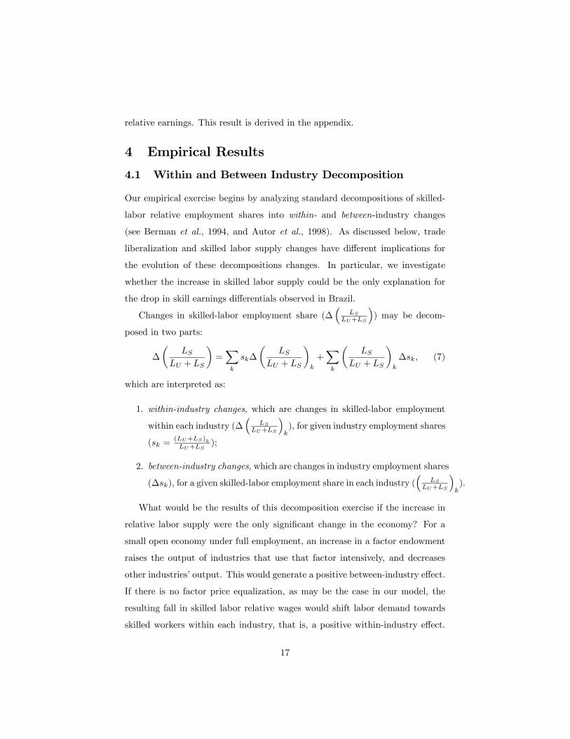
Our empirical exercise begins by analyzing standard decompositions of skilled-

labor relative employment shares into within- and between-industry changes

(see Berman et al., 1994, and Autor et al., 1998). As discussed below, trade

liberalization and skilled labor supply changes have di¤erent implications for

the evolution of these decompositions changes. In particular, we investigate

whether the increase in skilled labor supply could be the only explanation for

the drop in skill earnings di¤erentials observed in Brazil.

Changes in skilled-labor employment share (��

LSLU+LS

�) may be decom-

posed in two parts:

�

�LS

LU + LS

�=Xk

sk�

�LS

LU + LS

�k

+Xk

�LS

LU + LS

�k

�sk, (7)

which are interpreted as:

1. within-industry changes, which are changes in skilled-labor employment

within each industry (��

LSLU+LS

�k), for given industry employment shares

(sk =(LU+LS)kLU+LS

);

2. between-industry changes, which are changes in industry employment shares

(�sk), for a given skilled-labor employment share in each industry (�

LSLU+LS

�k).

What would be the results of this decomposition exercise if the increase in

relative labor supply were the only signi�cant change in the economy? For a

small open economy under full employment, an increase in a factor endowment

raises the output of industries that use that factor intensively, and decreases

other industries�output. This would generate a positive between-industry e¤ect.

If there is no factor price equalization, as may be the case in our model, the

resulting fall in skilled labor relative wages would shift labor demand towards

skilled workers within each industry, that is, a positive within-industry e¤ect.

17

In terms of equation (7), an increase in skilled-labor supply is represented by

a positive left hand side. The two terms on the right hand side should also

positive, representing the positive within- and between-industry e¤ects.

What would be the results of this exercise if trade were the only source

behind the changes in earnings inequality? As described in Section 3, trade

opening should have caused a decrease in relative prices of skill-intensive sectors

in order to produce the observed decrease in earnings inequality.12 On the one

hand, these price incentives would decrease production in those sectors, which

denote a negative between-industry e¤ect. On the other hand, as above, the

relative wage incentives would yield a positive within-industry e¤ect. With

given factor supplies, the two e¤ects should o¤set each other.

Table 2 presents the skilled-labor employment share decomposition results,

using education attainment as a measure of skill from the PNAD dataset. Con-

�rming the labor supply movements displayed in Figure 3, skilled-labor em-

ployment share (measured by the high-school threshold) increased 2.67% a year

between 1988 and 1995, on average. The decomposition reveals that the within

e¤ect is positive and the between e¤ect is negative, that is, employment shifted

from skilled- to unskilled-intensive sectors, and each sector increased its relative

share of skilled labor. Two important conclusions emerge: (1) labor supply

changes alone cannot account for these results, and (2) the results are compat-

ible with the trade explanation.13

Total Within Industry Between IndustrySkilled Labor 0.0267 0.0334 -0.0067

Employment Share (100%) (125%) (-25%)

Table 2: Employment and Wage Bill Shares Decompositions, 1988-95

12Note that we are considering an economy that is relatively abundant in unskilled labor.13Results not reported here, using nonproduction share from PIA as a proxy for skill, are also

compatible with trade. But in that case, they explain the increase in earnings di¤erentalsobserved for that skill measure. There was an average overall annual decrease of 0.7% innonproduction employment share. This was decomposed into a negative within-industry e¤ect(-1.4%), which outweighted a positive between-industry e¤ect (0.7%).

18

4.2 Consistency Checks

We perform some consistency check exercises to examine the causality path

predicted by trade theory. As discussed in Section 3, the following relationships

should be investigated to determine whether trade liberalization was responsible

for the decrease in skilled labor relative earnings observed in Brazil:

1. What was the pattern of relative price changes? To be consistent with the

decrease in earnings inequality, one should observe a decrease in the rela-

tive prices of the sectors that use skilled labor intensively. This should be

re�ected in the data through a negative correlation between price changes

and skill intensity.

2. What was the pattern of tari¤ reduction? If these changes in relative

prices, negatively correlated with skill intensity, were induced by trade lib-

eralization, one should observe that the most skill-intensive sectors expe-

rienced the largest tari¤ reductions and/or that in these sectors the tari¤s

reduction had a larger impact on prices. As equation (6) shows, tari¤s ad-

justed by the share of imported goods in each sector is the proper measure

to be used to investigate the impact of trade liberalization on prices, since

it captures both the tari¤ changes and the di¤erentiated pass-through ef-

fect. Therefore, one should test the correlation between skill intensity and

adjusted tari¤ changes.

3. Was the pattern of price changes induced by tari¤ changes? This can be

examined through the estimation of price changes equations based on the

relationship established in equation (5).

We investigate each of these questions in turn over the next three sub-

sections.

4.2.1 Prices and Skill Intensity

The �rst step is to check whether the pattern of price changes is consistent

with the observed decrease in skilled labor relative earnings. Figure 8 suggests

19

that, between 1988 and 1995, relative prices decreased in sectors with a higher

proportion of educated workers.

We test the correlation between prices and the sector skill intensity by esti-

mating:

� logPk� = �0� + �1 log

�LS

LU + LS

�k;��1

+ �k� , (8)

where Pk� is the wholesale price for sector k in year � , and�

LSLU+LS

�kis the

share of skilled labor employed in sector k. The pattern of price changes must

deliver a negative value for �1, in order to be consistent with the decrease in

skilled-labor relative earnings.

Figure 8: Price Changes (1988-1995) and Skill Shares (1988)

.

Cha

nge 

in P

rices

skill share0 .1 .2 .3 .4

16

16.5

17

17.5

minerals

non­methalic

metallurgymechanic

eletric material

transport

wood

furniture

paper graphicrubber

chemical

drugs

perfumary

plastic

text ileclothing

leather

coffeetobacco

beverages

Equation (8) is estimated using yearly observations from 1988 to 1995, for

a sample of 60 industries (PIA classi�cation). The Brazilian wholesale price

index (Índice de Preços por Atacado - Oferta Global, IPA-OG),14 collected by

the Fundação Getulio Vargas, was matched to the PIA aggregation. The skilled

labor share based on education attainment was computed from the 21-sectors�

PNAD data set. When this is the skill measure used, we correct the standard

errors of all coe¢ cients for the fact that this variable is more aggregated than

the dependent variables.

14The weight of each good in IPA-OG is given by the good�s transactions share of totalsector�s transactions. The latter is de�ned as the sum of the sector�s total production andimports.

20

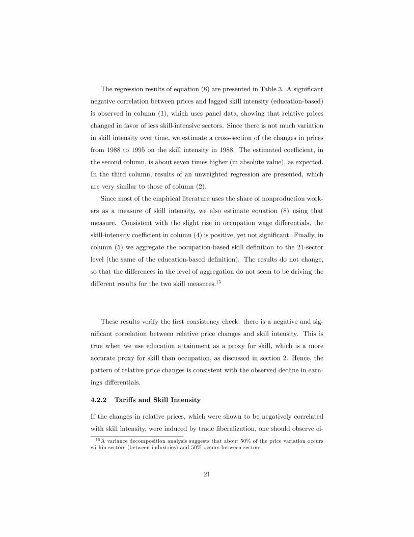
The regression results of equation (8) are presented in Table 3. A signi�cant

negative correlation between prices and lagged skill intensity (education-based)

is observed in column (1), which uses panel data, showing that relative prices

changed in favor of less skill-intensive sectors. Since there is not much variation

in skill intensity over time, we estimate a cross-section of the changes in prices

from 1988 to 1995 on the skill intensity in 1988. The estimated coe¢ cient, in

the second column, is about seven times higher (in absolute value), as expected.

In the third column, results of an unweighted regression are presented, which

are very similar to those of column (2).

Since most of the empirical literature uses the share of nonproduction work-

ers as a measure of skill intensity, we also estimate equation (8) using that

measure. Consistent with the slight rise in occupation wage di¤erentials, the

skill-intensity coe¢ cient in column (4) is positive, yet not signi�cant. Finally, in

column (5) we aggregate the occupation-based skill de�nition to the 21-sector

level (the same of the education-based de�nition). The results do not change,

so that the di¤erences in the level of aggregation do not seem to be driving the

di¤erent results for the two skill measures.15

These results verify the �rst consistency check: there is a negative and sig-

ni�cant correlation between relative price changes and skill intensity. This is

true when we use education attainment as a proxy for skill, which is a more

accurate proxy for skill than occupation, as discussed in section 2. Hence, the

pattern of relative price changes is consistent with the observed decline in earn-

ings di¤erentials.

4.2.2 Tari¤s and Skill Intensity

If the changes in relative prices, which were shown to be negatively correlated

with skill intensity, were induced by trade liberalization, one should observe ei-

15A variance decomposition analysis suggests that about 50% of the price variation occurswithin sectors (between industries) and 50% occurs between sectors.

21

Dependent Variable: Change in Prices(1) (2) (3) (4) (5)

High Education -0.043 -0.338 -0.299 - -Employment Share (0.020) (0.061) (0.131)

Nonproduction - - - 0.036 0.062Employment Share (0.239) (0.285)

Constant 3.489 16.240 16.320 16.913 16.947(0.039) (0.257) (0.241) (0.292) (0.355)

Observations 420 60 60 60 60Weighted Yes Yes No Yes Yes

Time Dummies Yes No No No NoNotes: Panel regression of yearly changes in column (1) and cross-sectionof 1988-1995 changes in columns (2) to (5). In column (5), nonproductionshare is aggregated to sector level. Sector employment shares are usedas weights. Robust standard errors are in parentheses.

Table 3: Prices and Skill Intensity, 1988-95

ther that the largest tari¤ reductions occurred in the most skill-intensive sectors

or that the pass-through from tari¤s to prices was larger in these sectors.

We �rst estimate the correlation between tari¤ changes and skill intensity

using the following equation:

� log (1 + tk� ) = 0� + 1 log

�LS

LU + LS

�k;��1

+ �k� , (9)

where tk is the average import tari¤ for sector k.

The results for cross-section long changes (1988-1995) regressions are pre-

sented in columns (1) and (2) of Table 4. Neither skill intensity measure is

signi�cantly correlated with the changes in tari¤s. Therefore, as already sug-

gested by Figure 7, there is no clear pattern of tari¤ reductions with relation to

skill intensity in Brazil.

According to equation (6), the proper measure to be used to investigate the

impact of trade liberalization on prices is tari¤s adjusted by the share of im-

ported goods in each sector. This measure captures both the tari¤ changes and

the di¤erentiated pass-through from tari¤s to prices. We, then, test the correla-

tion between adjusted tari¤ changes and skill intensity, using �k� log (1 + tk� )

22

as the dependent variable in equation (9), where �k is the import penetration.

This is measured as the ratio of imports over the sum of imports and total

production in each sector in the initial year (1988).

Columns (3) and (4) of Table 4 report the regression results for a panel

of yearly changes and for a cross-section of long changes, respectively. Both

skill-intensity coe¢ cients are negative and signi�cant, with the long-changes co-

e¢ cient being about six times larger (in absolute value) than the panel one as

expected. The unweighted regression yields the same result, as shown in column

(5). Interestingly, the use of nonproduction employment share as an alternative

explanatory variable also delivers a negative and statistically signi�cant coe¢ -

cient (see column (6)). These results indicate that adjusted tari¤s fell relatively

more in more skill-intensive sectors.

Dependent VariableChange in Tari¤s Change in Tari¤s*Import Shares(1) (2) (3) (4) (5) (6)

High Education -0.015 - -0.002 -0.012 -0.015 -Employment Share (0.023) (0.001) (0.004) (0.005)

Nonproduction - 0.002 - - - -0.008Employment Share (0.039) (0.004)

Constant -0.258 -0.252 -0.004 -0.031 -0.036 -0.019(0.038) (0.045) (0.001) (0.008) (0.009) (0.007)

Observations 60 60 420 60 60 60Weighted yes yes yes yes no yes

Time Dummies no no yes no no noNotes: Panel regression of yearly changes in column (3) and cross-section of1988-1995 changes in the other columns. Sector employment shares are usedas weights. Robust standard errors are in parentheses.

Table 4: Tari¤ Changes and Skill Intensity, 1988-95

Note that these last results contrast with those obtained in columns (1) and

(2), where tari¤ changes were not adjusted by import penetration. These two

sets of results together imply that: (i) tari¤ changes had no relationship with

skill intensity, and (ii) import penetration was larger in more skill-intensive

sectors, which, according to the arguments in section 3, entails a higher pass-

23

through from tari¤s to prices in these sectors.

This exercise establishes the second consistency check for the causality from

trade liberalization to earnings di¤erentials: adjusted tari¤ changes are nega-

tively correlated with skill intensity.

4.2.3 Prices and Tari¤s

We now investigate the relationship between tari¤ and price changes. Based on

equation (5), we estimate:

� logPk� = �0� + �1�k� log (1 + tk� ) + �2�k� logP�k� + "k� . (10)

�k captures the di¤erentiated pass-through impact from tari¤s to prices in sec-

tor k, measured by import penetration in 1988. As we do not have data on

goods international prices, we use sector international prices P �k� instead, prox-

ied by U.S. prices.16 �k, the di¤erentiated pass-through of international prices

to domestic sector prices, is measured by the ratio of imported plus exported

goods over the sum of production and total imports in the sector, which we

denote trade exposure.17

We have assumed away export subsidies and quantitative trade restric-

tions.18 Hence, changes in the rents generated by other trade barriers should

be captured by an error term, "k� . The e¤ects of other omitted variables are in

the time dummies and the error term.

Equation (10) is estimated using a panel of yearly observations from 1988

to 1995, for a sample of 50 industries. The level of aggregation is lower here

because we could only match 50 U.S. industries to the PIA classi�cation. U.S.

producer price data are from the Bureau of Labor Statistics. In order to identify

the causal e¤ect of tari¤s on prices, we must assume that the tari¤s changes

16Note that equation (5) considered international prices as measured by the same currencyas domestic prices. Were they measured by another currency, any nominal exchange ratechanges would be captured by the time dummies �0� .17 In equation (5), we split the sector into domestically produced and imported goods. How-

ever, the domestically produced goods include both nontraded and exported goods, and theprices of the latter also depend on international prices.18As discussed in Section 2.2, most non-tari¤ barriers were replaced by tari¤s in the outset

of trade liberalization.

24

are exogenous, that is, not correlated to other (omitted) determinants of price

changes. Note, however, that this was a period of substantial policy changes in

Brazil. We argue that the introduction of time dummies in equation (10) absorbs

the contemporaneous correlation between changes in tari¤s and the other policy

changes, which is true as long as there is no within-sector correlation among

these changes.

We �rst estimate equation (10) without considering the di¤erentiated pass-

through coe¢ cient, that is, we regress price changes on unadjusted tari¤ changes

and U.S. prices changes (with �k = 1 and �k = 1, 8k). The �rst column

of Table 5 presents the estimation results using panel data. The estimated

tari¤ coe¢ cient is positive and statistically di¤erent from zero at conventional

signi�cance levels. The coe¢ cient for U.S. prices is not precisely estimated in

this speci�cation. In the long di¤erences regression, presented in the second

column, neither coe¢ cient is signi�cantly di¤erent from zero.

Next, we take into account the di¤erentiated pass-through coe¢ cients from

tari¤s and from international prices to domestic industry prices, as in equation

(10). We regress the prices changes on the tari¤s changes multiplied by import

penetration, �k, and U.S. price changes times trade exposure, �k. Both �k and

�k are measured by 1988 levels. The results of the panel regression, reported

in column (3), show that the coe¢ cient of adjusted tari¤ changes is also posi-

tive and statistically signi�cant. Moreover, adjusted international prices turned

out to be positive and signi�cant.19 In column (4) we use the long-di¤erences

speci�cation and �nd that the coe¢ cient of adjusted tari¤s is positive but not

signi�cant at conventional levels. In an unweighted regression, in column (5),

the coe¢ cients of both the adjusted tari¤s and adjusted international prices

changes are positive and signi�cant.

These results are in accordance with the predictions of the model presented

in section 3: relative price changes are positively correlated with tari¤ changes

adjusted by import penetration and with international prices adjusted by trade

19One cannot compare the magnitude of the estimated coe¢ cients because of the di¤erencesin the units of measurement between the two variables.

25

exposure.20

Dependent Variable: Price Changes(1) (2) (3) (4) (5)

Tari¤ Changes 0.457 0.125 - - -(0.237) (0.775)

Tari¤ Changes* - - 4.221 5.173 4.035Import Penetration (2.194) (3.821) (2.011)

U.S. Price Changes 0.105 1.446 - - -(0.182) (0.915)

U.S. Price Changes* - - 0.378 2.031 1.001Trade Exposure (0.155) (1.919) (0.472)

Constant 2.882 16.684 2.874 16.857 16.869(0.018) (0.215) (0.018) (0.075) (0.070)

Observations 350 50 350 50 50Weighted yes yes yes yes no

Time Dummies yes no yes no noNotes: Panel regression of yearly changes in columns (1) and (3) and cross-sectionof 1988-1995 changes in the other columns. Sector employment shares are usedas weights. Robust standard errors are in parentheses.

Table 5: Price Changes and Tari¤ Changes, 1988-95

4.3 Mandated Wage Equations

While the pattern of price changes is consistent with the pattern of relative earn-

ings evolution and correlated with tari¤ changes, we have not as yet examined

how much of the drop in skill earnings di¤erentials could be attributed to price

changes mandated by trade liberalization. We therefore follow another vein of

the trade literature and estimate mandated wage equations (see Baldwin and

Cain, 1997, Haskel and Slaughter, 2002, and Robertson, 2004). According to

the Stolper-Samuelson theorem, price changes should equal factor price changes,20There is one caveat in interpreting the results of this regression. The composition of goods

within each sector may change over time, and this change may be correlated with changes intrade policy. On the one hand, trade liberalization may reduce or even eliminate domesticproduction of goods with relatively high domestic production costs. On the other hand, newproducts may be introduced due to the reduced cost of imported goods. Even though this isa drawback, there is nothing we can do to correct for possible measurement errors caused byit.

26

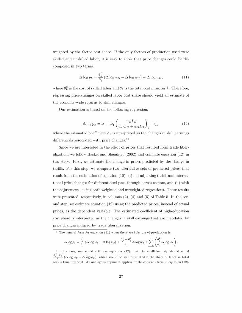
weighted by the factor cost share. If the only factors of production used were

skilled and unskilled labor, it is easy to show that price changes could be de-

composed in two terms:

� log pk =�Sk�k(� logwS �� logwU ) + � logwU , (11)

where �Sk is the cost of skilled labor and �k is the total cost in sector k. Therefore,

regressing price changes on skilled labor cost share should yield an estimate of

the economy-wide returns to skill changes.

Our estimation is based on the following regression:

� log pk = �0 + �1

�wSLS

wULU + wSLS

�k

+ �k, (12)

where the estimated coe¢ cient �1 is interpreted as the changes in skill earnings

di¤erentials associated with price changes.21

Since we are interested in the e¤ect of prices that resulted from trade liber-

alization, we follow Haskel and Slaughter (2002) and estimate equation (12) in

two steps. First, we estimate the change in prices predicted by the change in

tari¤s. For this step, we compute two alternative sets of predicted prices that

result from the estimation of equation (10): (i) not adjusting tari¤s and interna-

tional price changes for di¤erentiated pass-through across sectors, and (ii) with

the adjustments, using both weighted and unweighted regressions. These results

were presented, respectively, in columns (2), (4) and (5) of Table 5. In the sec-

ond step, we estimate equation (12) using the predicted prices, instead of actual

prices, as the dependent variable. The estimated coe¢ cient of high-education

cost share is interpreted as the changes in skill earnings that are mandated by

price changes induced by trade liberalization.

21The general form for equation (11) when there are l factors of production is:

�log pj =�1j

�j(� logw1 �� logw2) +

�1j + �2j

�j� logw2 +

lXk=3

�kj

�j� logwk

!.

In this case, one could still use equation (12), but the coe¢ cient �1 should equal�Sj +�

Uj

�j(� logwS �� logwU ), which would be well estimated if the share of labor in total

cost is time invariant. An analogous argument applies for the constant term in equation (12).

27

Dependent Variable: Change in PricesPredicted by tari¤

Predicted changes, adjusted byby tari¤ changes di¤. pass-through

(1) (2) (3)High-Education Cost Share -0.048 -0.294 -0.268

(0.039) (0.085) (0.088)

Constant 16.88 16.93 16.94(0.021) (0.087) (0.033)

Auxiliary Regression in Table 5 Col.(2) Col.(4) Col.(5)Actual Change in Log Earnings Di¤s -0.168 -0.168 -0.168

Observations 60 60 60Weighted Original Regressions yes yes no

Notes: Robust standard errors are in parentheses.

Table 6: Mandated Wages

The results are presented in Table 6. The actual fall in skill earnings di¤eren-

tials observed in Brazil from 1988 to 1995 was 15.5% (which corresponds to the

-0.168 log di¤erence). The �rst column shows that the decline in earnings dif-

ferentials mandated by the price variation predicted by the (unadjusted) change

in tari¤s was estimated at 4.7%, but was not signi�cantly di¤erent from zero.

When we use the price changes predicted by tari¤s, allowing for di¤erentiated

pass-through coe¢ cients across sectors, weighted in column (2) and unweighted

in column (3), we �nd mandated annualized skill earnings di¤erential declines

of 25.5% (-0.294 log di¤erence) and 23.5% (-0.268), respectively.

These results indicate that, if trade were the only change in the Brazilian

economy from 1988 to 1995, skill earnings di¤erentials would have fallen by even

more (8-10 percentage points) than what was actually observed. Other changes

in the economy were responsible for this di¤erence. In particular, skill biased

technological changes would have had a positive impact on the di¤erentials.

Note, however, that the observed labor supply changes might have reinforced

the decline in earnings di¤erentials. It is beyond the scope of this paper to

disentangle the contribution of these other factors on the evolution of the skill

premium. Nevertheless, this result provides compelling evidence that trade

28

liberalization played a major role in explaining the decrease in skilled labor

relative earnings in Brazil.

5 Conclusion

During the trade liberalization implemented in Brazil from 1988 to 1995, earn-

ings of workers with at least complete high school decreased with respect to

earnings of less educated workers. In this paper we present evidence compat-

ible with trade liberalization having played a role in explaining these relative

earnings movements.

First, a decomposition analysis of changes in skilled-labor employment share

over this period reveals that employment shifted from skilled- to unskilled-

intensive sectors, and that each sector increased its relative share of skilled

labor. Second, we show that relative prices fell in skill-intensive sectors, and

that tari¤s reductions, adjusted by import penetration, were larger in those

sectors. Furthermore, we �nd not only that prices and tari¤s were positively

correlated, but also that the impact of tari¤s changes on prices was higher in sec-

tors with larger import penetration. Finally, we show that the decline in skilled

earnings di¤erentials mandated by the price variation predicted by trade, allow-

ing for di¤erentiated pass-through coe¢ cients across sectors, was even larger

than the observed one. In sum, all steps of the trade transmission mechanism

were tested, and the results are compatible with trade liberalization accounting

for the observed relative earnings changes in Brazil.

Our results highlight the importance of considering the e¤ects of di¤eren-

tiated pass-through from tari¤s to prices across sectors in order to adequately

investigate the e¤ects of trade liberalization on relative prices. We develop a

theoretical foundation for this through a modi�ed version of Dornbusch et al.

(1980), which shows that the pass-through from tari¤s to prices in each sector

depends on the sector�s import penetration.

29

References

[1] Acemoglu, D.(2002). �Technical Change, Inequality and the Labor Mar-ket,�Journal of Economic Literature, 50 (1), 7-72.

[2] Acemoglu, D.(2003). �Patterns of Skill Premia,�Review of Economic Stud-ies, 70, 199-230.

[3] Autor, D., L.Katz and A.Krueger (1998). �Computing Inequality: HaveComputers Changed the Labor Market?,�The Quarterly Journal of Eco-nomics, 113(4): 1169-213.

[4] Baldwin, R. and G.Cain (1997). �Shifts in U.S. Relative Wages: The Roleof Trade, Technology and Factor Endowments,� NBER Working Paper#5934.

[5] Behrman, J., N.Birdsall and M.Székely (2000). �Economic Reform andWage Di¤erentials in Latin America,�Inter-American Development Bank,Working Paper #435.

[6] Berman, E., J.Bound and Z.Griliches (1994). �Changes in the Demand forSkilled Labor within US Manufacturing: Evidence from the Annual Surveyof Manufacturers,�The Quarterly Journal of Economics, 109(2): 367-98.

[7] Beyer, H., P.Rojas, and R.Vergara (1999). �Trade Liberalization and WageInequality,�Journal of Development Economics, 59: 103-23.

[8] Dornbusch, R., S.Fischer and P.Samuelson (1980). �Heckscher-Ohlin TradeTheory with a Continuum of Goods,�The Quarterly Journal of Economics,95(2): 203-24.

[9] Hanson, G. and A.Harrison (1999). �Trade Liberalization and Wage In-equality in Mexico,�Industrial and Labor Relations Review, 52(2): 272-88.

[10] Haskel, J. and M.Slaughter (2003). �Have Falling Tari¤s and Transporta-tion Costs Raised U.S. Wage Inequality?,�Review of International Eco-nomics,11(4): 630-50.

[11] Duryea, S., R.Robertson and W.Hernani (2002). �Regional Integrationand Wage Inequality,�in Beyond Borders: The New Regionalism in LatinAmerica, Inter-American Development Bank.

[12] Krueger, A.(1997). �Labor Market Shifts and The Price Puzzle Revisited,�NBER Working Paper #5924.

30

[13] Kume, H.(2002). �A política brasileira de importação no período 1987-99:descrição e avaliação,�May, mimeo.

[14] Muendler, M., J.Poole, G.Ramey and T.Wajnberg (2004). �Job Concor-dances in Brazil: Mapping the Classi�cação Brasileira de Ocupações to theInternational Standard Classi�cation of Occupations�, UCSD, mimeo.

[15] Robertson, R.(2004). �Relative Prices and Wage Inequality: Evidence fromMexico,�Journal of International Economics, 64(2): 387-409.

[16] Romalis, J.(2004). �Factor Proportions and the Structure of CommodityTrade,�The American Economic Review, 94(1): 67-97.

[17] Slaughter, M.(2000). �What are the Results of Product-Prices Studies andWhat Can We Learn from Their Di¤erences?,� in Robert Feenstra (ed.),The Impact of International Trade on Wages, NBER Conference Report,Chicago: University of Chicago Press, 129-70.

[18] Thoenig, M. and T.Verdier (2003).�A Theory of Defensive Skill-Biased In-novation and Globalization,�American Economic Review, 93(3):709-28.

6 Appendix

6.1 Stolper-Samuelson Result and the E¤ect of Labor Sup-ply Changes

Stolper-Samuelson Result We start by deriving the Stolper-Samuelsonresult in the model developed in section 3. This can more easily be shown ina simpli�ed version of the model with no sectorial aggregation of goods, thatis, assuming q (k; z) � q (z).22 Cuto¤ points z and z can still be obtained fromequations (2) and (3). Equilibrium in this economy is characterized by balancedtrade and by full employment of both factors.Balanced trade requires that:Z z

0

b (z) (w�L�U + s�L�S) dz =

Z 1

z

b (z) (wLU + sLS)

1 + �dz; (13)

where b (k) is the proportion of income spent on sector-k goods, assuming Cobb-Douglas consumer preferences, LU (L�U ) and LS (L

�S) are unskilled and skilled

labor supplies in the South (North), and tari¤s � are the same for all goods. To

22Using the sectorial aggregation yields the same results as in this appendix, although theequations are much more cumbersome.

31

obtain equation (13), we use the fact that preferences imply that the demandfor good z by Southern consumers is:

q (z) =b (z) (wLU + sLS)

pd (z); (14)

with an equivalent equation for the North.The condition for skilled labor full employment in South is given by:

LS =

Z z

0

�zw

(1� z) s

�1�zb (z)

p (z)(wLU + sLS + w

�L�U + s�L�S) dz+ (15)

+

Z z

z

�zw

(1� z) s

�1�zb (z)

p (z)(wLU + sLS) dz;

which follows from the demand for skilled labor equation,23

LS (z) =

�zw

(1� z) s

�1�z[q (z) + q� (z)] ;

and uses the demand conditions in equation (14) and the fact that pc (z) = p (z)(see footnote 9). Analogously, the full employment equation for unskilled laboris:

LU =

Z z

0

�zw

(1� z) s

��zb (z)

p (z)(wLU + sLS + w

�L�U + s�L�S) dz+ (16)

+

Z z

z

�zw

(1� z) s

��zb (z)

p (z)(wLU + sLS) dz:

Substituting the balanced trade condition into equations (15) and (16), andsimplifying using the zero pro�t conditions as in Dornbusch et al. (1980), weget:

�ls =

Z z

0

b (z) (� + ls)

(� + ls (z))ls (z) dz + �

Z z

z

b (z) (� + ls)

(� + ls (z))ls (z) dz; (17)

for skilled labor, and:

� =

Z z

0

b (z) (� + ls)

(� + ls (z))dz + �

Z z

z

b (z) (� + ls)

(� + ls (z))dz; (18)

for unskilled labor, where � � (1+�)R z0b(z)dz

(1+�)R z0b(z)dz+

R 1zb(z)dz

, � � ws , ls (z) �

Ls(z)Lu(z)

=

z�(1�z) and ls �

LsLu. Combining equations (17) and (18), we get:

F (�; �) �Z z

0

b (z) [z� � (1� z) ls] dz+�Z z

z

b (z) [z� � (1� z) ls] dz = 0: (19)

23 In this simpli�ed version, we assume A (k) = 1.

32

An analogous equation can be derived for the North. With equation (19) andits counterpart for the North one can derive relative wages in the two countries(� and ��).In this set up, the Stolper-Samuelson result is equivalent to d�

d� < 0, thatis, trade liberalization in South yields an increase in the relative wages of un-skilled labor, its relatively abundant factor. This can be derived by applyingthe implicit function theorem to equation (19).The numerator of d�d� is:

@F (�; �)

@�=

@�

@�

Z z

z

b (z) (� + ls) [z� � (1� z) ls] dz + (20)

� �

(1 + �) log (�=��)b (z) (� + ls) [z� � (1� z) ls] ;

where:

@�

@�=� (1� �)1 + �

� �b (z)

(1 + �) log (�=��)h(1 + �)

R z0b (z) dz +

R 1zb (z) dz

i :First, note that log (�=��) < 0 (see footnote 8), hence, @�

@� > 0. Second,R zzb (z) (� + ls) [z� � (1� z) ls] dz > 0, for the following reason. This expres-

sion is in the second term of F (�; �) in equation (19). As F (�; �) = 0, eitherits two terms are zero, or one is positive and the other is negative. It cannot bethe case that both are zero, since [z� � (1� z) ls] is monotonically increasing inz. This monotonicity also implies that the �rst term cannot be positive. Hence,the only possibility is the �rst term being negative and the second positive.Therefore, we can establish that @F (�;�)@� > 0.Finally, the second term in equation (20) is positive, as we show by contradic-

tion that [z� � (1� z) ls] is positive. Note that z��(1� z) ls = [ls (z)� ls] (1� z) :Suppose that ls (z)� ls < 0. Due to its monotonicity in z, we would have thatls (z) � ls < 0; 8z � z, that is, for all goods produced in the country. The fullemployment in the economy implies that relative labor demand equals relative

labor supply, that is,R z0LS(z)dzR z

0LU (z)dz

= ls: The relative labor demand can be rewrit-

ten asR z0ls(z)LU (z)dzR z0LU (z)dz

, which would be smaller thanR z0lsLU (z)dzR z

0LU (z)dz

= ls, under the

assumption ls (z) < ls. Hence, we would have a contradiction.

33

The denominator of d�d� is:

@F (�; �)

@�=

F (�; �)

� + ls+

Z z

0

b (z) (� + ls) zdz + �

Z z

z

b (z) (� + ls) zdz +(21)

+(� � 1) z

� log (�=��)b (z) (� + ls) [z� � (1� z) ls] +

� �z

� log (�=��)b (z) (� + ls) [z� � (1� z) ls] :

The �rst term in equation (21) is zero, and the second and third are positive.We have already shown that the last term is positive.The fourth term may be either positive or negative. If ls (z) � ls < 0, then

the term is positive and @F (�;�)@� > 0. Otherwise, we can derive the following

necessary and su¢ cient condition for @F (�;�)@� > 0, assuming b (z) constant for

all z:24

z > �"z2 (1 + �)

(1� z) +ls (1 + �z) = (1� z)� log(�=��)

2 � (� + ls)

#:

We have that both @F (�;�)@� > 0 and @F (�;�)

@� > 0, then d�d� < 0, yielding the

Stolper-Samuelson result.

The E¤ect of Labor Supply Changes The e¤ect of labor supply changesis straighforward. We apply the implicit function theorem to equation (19) toderive d�

dls. Its denominator, @F (�;�)

@� , is the same as in d�d� . We have argued

above that, under certain conditions, it is positive.The denominator of d�dls is:

dF (�; �)

dls=F (�; �)

� + ls+

Z z

0

b (z) (� + ls) (z � 1) dz+�Z z

z

b (z) (� + ls) (z � 1) dz:

(22)The �rst term in equation (22) is zero and the other two terms are negative.Hence, we have that d�

dls> 0, that is, an increase in skilled-labor relative supply

decreases skilled-labor relative earnings.

24Note that, if ls (z) � ls > 0, the sign of @F (�;�)@�

can only be established with somerestriction on the behavior of b (z). It is reasonable to assume that b (z) is well behaved.

34

6.2 Data Matching

Industry: PIA Sector: PNAD1 Metal Ore Mining Minerals2 Cement Manufacturing Minerals non­metallic3 Cement, Concrete and Gypsum Product Manufacturing Minerals non­metallic4 Glass and Glass Product Manufacturing Minerals non­metallic5 Nonmetallic Mineral Product Manufacturing Minerals non­metallic6 Iron Production and Processing Metallurgy7 Nonferrous Metals Production and Processing Metallurgy8 Steel Production and Processing Metallurgy9 Other Metal Products Manufacturing Metallurgy

10 Machinery, Equipment and Commercial Installation Manufacturing Mechanic11 Road Construction Machinery and Tractor Manufacturing Mechanic12 Machinery Maintenance, Repairing and Installation Mechanic13 Electrical Products Manufacturing for Power Generation and Distribution Electrical material14 Electric Conductor and Other Electrical Device Manufacturing Electrical material15 Electric Appliance and Equipment Manufacturing (including household appliances) Electrical material16 Electronic Components, Electronic Equipment and Communication Apparatus Manufact Electrical material17 Audio and Video Equipment Manufacturing Electrical material18 Automobile, Truck and Bus Manufacturing Transport19 Motor Vehicle Engine and Parts Manufacturing Transport20 Ship and Boat Building (including repairing) Transport21 Railroad Rolling Stock Manufacturing and Repairing Transport22 Other Transportation Equipment Manufacturing Transport23 Wood Sawing and Wood Products Manufacturing Wood24 Furniture Manufacturing Furniture25 Pulp and Paper Production Paper26 Pulp, Paper and Paperboard Products Manufacturing Paper27 Printing, publishing and allied industries Graphic28 Rubber Product Manufacturing Rubber29 Non­petrochemical Chemical Manufacturing Chemicals30 Alcohol Production Chemicals31 Petroleum Refining Chemicals32 Basic and Intermediate Petrochemical Manufacturing Chemicals33 Resins, Artificial and Synthetic Fibers and Elastomers Manufacturing Chemicals34 Fertilizer Manufacturing Chemicals35 Miscellaneous Chemical Product Manufacturing Chemicals36 Pharmaceutical Manufacturing Drugs37 Perfumes, Detergents and Candles Manufacturing Perfumery38 Laminated Plastics Plate and Pipe Manufacturing Plastic39 Plastics Products Manufacturing Plastic40 Natural Fabric Processing, Weaving, Knitting and Finishing" Textile41 Artificial and Synthetic Fabric Weaving, Knitting and Coating" Textile42 Other Textiles Manufacturing Textile43 Apparel and Apparel Accessories Manufacturing Clothing44 Leather and Hide Products and Luggage Manufacturing" Leather45 Footwear Manufacturing Leather46 Coffee Manufacturing Food47 Rice Milling and Processing Food48 Wheat Milling Food49 Fruit and Vegetable Processing and Canning Food50 Other Grains and Seeds Milling and Plant Product Manufacturing Food51 Tobacco Product Manufacturing Tobacco52 Animal (except poultry) Slaughtering and Meat Processing Food53 Poultry Slaughtering and Processing Food54 Fluid Milk and Dairy Product Manufacturing Food55 Sugar Manufacturing Food56 Oilseed Milling Food57 Seed Oil Refining and Food Fats and Oils Processing Food58 Animal Feeds Manufacturing Food59 Other Food Manufacturing Food60 Beverage Manufacturing Beverages

Data matching: PIA vs. PNAD

35

Departamento de Economia PUC-Rio

Pontifícia Universidade Católica do Rio de Janeiro Rua Marques de Sâo Vicente 225 - Rio de Janeiro 22453-900, RJ

Tel.(21) 31141078 Fax (21) 31141084 www.econ.puc-rio.br flavia@econ.puc-rio.br