No Contagion, Only Interdependence: Measuring Stock Market … · 2015-03-02 · Figure 2. Stock market indices during the 1994 Mexican crisis. This figure graphs stock market indices

No Contagion, Only Interdependence:Measuring Stock Market Comovements

KRISTIN J. FORBES and ROBERTO RIGOBON*

ABSTRACT

Heteroskedasticity biases tests for contagion based on correlation coefficients. Whencontagion is defined as a significant increase in market comovement after a shockto one country, previous work suggests contagion occurred during recent crises.This paper shows that correlation coefficients are conditional on market volatility.Under certain assumptions, it is possible to adjust for this bias. Using this adjust-ment, there was virtually no increase in unconditional correlation coefficients ~i.e.,no contagion! during the 1997 Asian crisis, 1994 Mexican devaluation, and 1987U.S. market crash. There is a high level of market comovement in all periods,however, which we call interdependence.

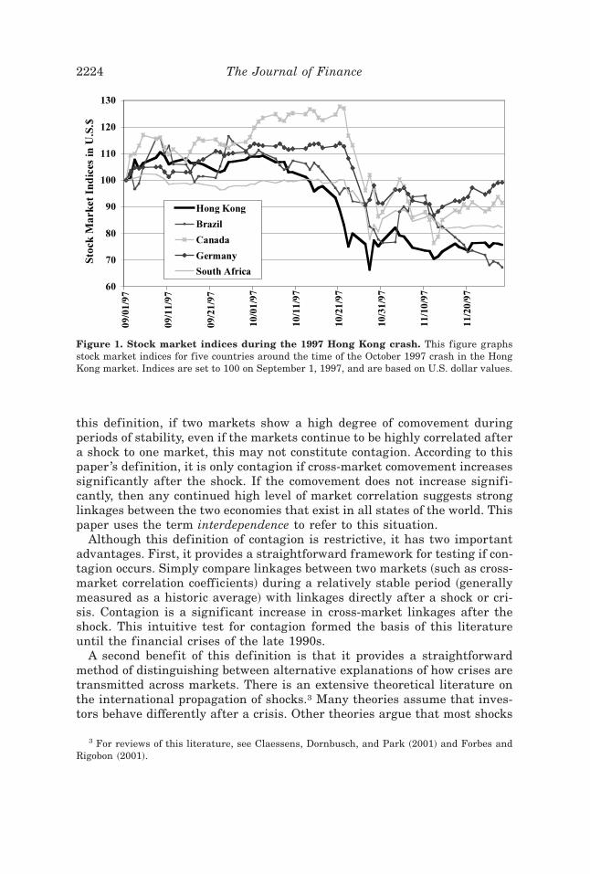
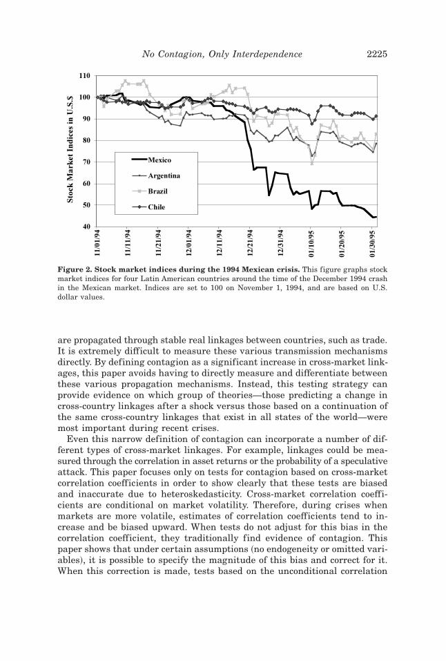
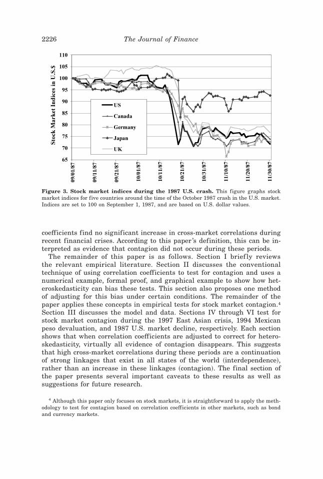
IN OCTOBER 1997, THE HONG KONG STOCK MARKET declined sharply and thenpartially rebounded. As shown in Figure 1, this movement affected marketsin North and South America, Europe, and Africa. In December 1994, theMexican market dropped significantly, and as shown in Figure 2, this fallwas quickly ref lected in other Latin American markets. Figure 3 shows thatin October 1987, the U.S. market crash affected major stock markets aroundthe world. These cases show that dramatic movements in one stock marketcan have a powerful impact on markets of very different sizes and structuresacross the globe. Do these periods of highly correlated stock market move-ments provide evidence of contagion?

Before answering this question, it is necessary to define contagion. Thereis widespread disagreement about what this term entails, and this paperutilizes a narrow definition that has historically been used in this litera-ture.1 This paper defines contagion as a significant increase in cross-marketlinkages after a shock to one country ~or group of countries!.2 According to

* Forbes and Rigobon are both from the Sloan School of Management at the MassachusettsInstitute of Technology. Thanks to Rudiger Dornbusch; Richard Greene; Andrew Rose; JaumeVentura; an anonymous referee; and seminar participants at Dartmouth, MIT, and NYU forhelpful comments and suggestions.

1 For a discussion of alternate def initions and their advantages and disadvantages,see Forbes and Rigobon ~2001! or the web site http:00www.worldbank.org0economicpolicy0managing%20volatility0contagion0Definitions_of_Contagion0definitions_of_contagion.html.

2 It is important to note that this definition of contagion is not universally accepted. Someeconomists argue that contagion occurs whenever a shock to one country is transmitted toanother country, even if there is no significant change in cross-market relationships. Othersargue that it is impossible to define contagion based on changes in cross-market linkages.Instead, they argue that it is necessary to identify exactly how a shock is propagated acrosscountries, and only certain types of transmission mechanisms ~no matter what the magnitude!constitute contagion.

THE JOURNAL OF FINANCE • VOL. LVII, NO. 5 • OCTOBER 2002

2223

this definition, if two markets show a high degree of comovement duringperiods of stability, even if the markets continue to be highly correlated aftera shock to one market, this may not constitute contagion. According to thispaper ’s definition, it is only contagion if cross-market comovement increasessignificantly after the shock. If the comovement does not increase signifi-cantly, then any continued high level of market correlation suggests stronglinkages between the two economies that exist in all states of the world. Thispaper uses the term interdependence to refer to this situation.

Although this definition of contagion is restrictive, it has two importantadvantages. First, it provides a straightforward framework for testing if con-tagion occurs. Simply compare linkages between two markets ~such as cross-market correlation coefficients! during a relatively stable period ~generallymeasured as a historic average! with linkages directly after a shock or cri-sis. Contagion is a significant increase in cross-market linkages after theshock. This intuitive test for contagion formed the basis of this literatureuntil the financial crises of the late 1990s.

A second benefit of this definition is that it provides a straightforwardmethod of distinguishing between alternative explanations of how crises aretransmitted across markets. There is an extensive theoretical literature onthe international propagation of shocks.3 Many theories assume that inves-tors behave differently after a crisis. Other theories argue that most shocks

3 For reviews of this literature, see Claessens, Dornbusch, and Park ~2001! and Forbes andRigobon ~2001!.

Figure 1. Stock market indices during the 1997 Hong Kong crash. This figure graphsstock market indices for five countries around the time of the October 1997 crash in the HongKong market. Indices are set to 100 on September 1, 1997, and are based on U.S. dollar values.

2224 The Journal of Finance

are propagated through stable real linkages between countries, such as trade.It is extremely difficult to measure these various transmission mechanismsdirectly. By defining contagion as a significant increase in cross-market link-ages, this paper avoids having to directly measure and differentiate betweenthese various propagation mechanisms. Instead, this testing strategy canprovide evidence on which group of theories—those predicting a change incross-country linkages after a shock versus those based on a continuation ofthe same cross-country linkages that exist in all states of the world—weremost important during recent crises.

Even this narrow definition of contagion can incorporate a number of dif-ferent types of cross-market linkages. For example, linkages could be mea-sured through the correlation in asset returns or the probability of a speculativeattack. This paper focuses only on tests for contagion based on cross-marketcorrelation coefficients in order to show clearly that these tests are biasedand inaccurate due to heteroskedasticity. Cross-market correlation coeffi-cients are conditional on market volatility. Therefore, during crises whenmarkets are more volatile, estimates of correlation coefficients tend to in-crease and be biased upward. When tests do not adjust for this bias in thecorrelation coefficient, they traditionally find evidence of contagion. Thispaper shows that under certain assumptions ~no endogeneity or omitted vari-ables!, it is possible to specify the magnitude of this bias and correct for it.When this correction is made, tests based on the unconditional correlation

Figure 2. Stock market indices during the 1994 Mexican crisis. This figure graphs stockmarket indices for four Latin American countries around the time of the December 1994 crashin the Mexican market. Indices are set to 100 on November 1, 1994, and are based on U.S.dollar values.

No Contagion, Only Interdependence 2225

coefficients find no significant increase in cross-market correlations duringrecent financial crises. According to this paper ’s definition, this can be in-terpreted as evidence that contagion did not occur during these periods.

The remainder of this paper is as follows. Section I brief ly reviewsthe relevant empirical literature. Section II discusses the conventionaltechnique of using correlation coefficients to test for contagion and uses anumerical example, formal proof, and graphical example to show how het-eroskedasticity can bias these tests. This section also proposes one methodof adjusting for this bias under certain conditions. The remainder of thepaper applies these concepts in empirical tests for stock market contagion.4Section III discusses the model and data. Sections IV through VI test forstock market contagion during the 1997 East Asian crisis, 1994 Mexicanpeso devaluation, and 1987 U.S. market decline, respectively. Each sectionshows that when correlation coefficients are adjusted to correct for hetero-skedasticity, virtually all evidence of contagion disappears. This suggeststhat high cross-market correlations during these periods are a continuationof strong linkages that exist in all states of the world ~interdependence!,rather than an increase in these linkages ~contagion!. The final section ofthe paper presents several important caveats to these results as well assuggestions for future research.

4 Although this paper only focuses on stock markets, it is straightforward to apply the meth-odology to test for contagion based on correlation coefficients in other markets, such as bondand currency markets.

Figure 3. Stock market indices during the 1987 U.S. crash. This figure graphs stockmarket indices for five countries around the time of the October 1987 crash in the U.S. market.Indices are set to 100 on September 1, 1987, and are based on U.S. dollar values.


I. Empirical Evidence on International Transmission Mechanisms

As discussed above and shown in Figures 1–3, stock markets of verydifferent sizes, structures, and geographic locations can exhibit a high de-gree of comovement after a shock to one market. Since stock markets dif-fer greatly across countries, this high degree of comovement suggests theexistence of mechanisms through which domestic shocks are transmittedinternationally. The empirical literature testing how shocks are propagatedand if contagion exists is extensive.5 Much of this empirical literature usesthe same definition of contagion as in this paper, although some of themore recent work has used a broader definition. Four different methodol-ogies have been utilized to measure how shocks are transmitted internation-ally: cross-market correlation coefficients, ARCH and GARCH models,cointegration techniques, and direct estimation of specific transmission mech-anisms. Many of these papers do not explicitly test for contagion, but vir-tually all papers which do test for its existence conclude that contagion—nomatter how defined—occurred during the crisis under investigation.

The first methodology uses cross-market correlation coefficients and isthe most straightforward approach to test for contagion. These tests mea-sure the correlation in returns between two markets during a stable periodand then test for a significant increase in this correlation coefficientafter a shock. If the correlation coefficient increases significantly, this sug-gests that the transmission mechanism between the two markets strength-ened after the shock and contagion occurred. In the first major paper usingthis approach, King and Wadhwani ~1990! test for an increase in stockmarket correlations between the United States, the United Kingdom, andJapan and find that cross-market correlations increased significantlyafter the U.S. market crash in 1987. Lee and Kim ~1993! extend this analy-sis to 12 major markets and find further evidence of contagion; averageweekly cross-market correlations increased from 0.23 before the 1987 U.S.crash to 0.39 afterward. Calvo and Reinhart ~1996! use this approach totest for contagion in stock prices and Brady bonds after the 1994 Mexicanpeso crisis. They find that cross-market correlations increased for manyemerging markets during the crisis. To summarize, each of these testsbased on cross-market correlation coefficients reaches the same generalconclusion: There was a statistically significant increase in cross-marketcorrelation coefficients during the relevant crisis and, therefore, contagionoccurred.6

5 For an excellent survey of this empirical literature, see Claessens et al. ~2001!. For a num-ber of recent empirical papers on this subject, see Claessens and Forbes ~2001!.

6 For further applications and extensions of this general approach, see Bertero and Mayer~1990! for a study of why the transmission of the U.S. stock market crash differed across coun-tries, Karolyi and Stulz ~1996! for an analysis of comovements between the U.S. and Japanesemarkets, Pindyck and Rotemberg ~1993! for a study of comovements between individual stockprices within the United States, and Pindyck and Rotemberg ~1990! for an analysis of comove-ments in commodity prices.


A second approach for analyzing market comovement is to use an ARCHor GARCH framework to estimate the variance–covariance transmissionmechanisms between countries. Hamao, Masulis, and Ng ~1990! use thisprocedure to examine stock markets around the 1987 U.S. stock marketcrash and find evidence of significant price-volatility spillovers from NewYork to London and Tokyo, and from London to Tokyo. Edwards ~1998!examines linkages between bond markets after the Mexican peso crisis andshows that there were significant spillovers from Mexico to Argentina, butnot from Mexico to Chile. Both of these papers, along with most otherstudies based on ARCH and GARCH models, show that market volatility istransmitted across countries. They do not, however, explicitly test if thistransmission changes significantly after the relevant shock or crisis. There-fore, although these papers provide important evidence that volatility istransmitted across markets, most do not explicitly test for contagion asdefined in this paper.

A third method of examining cross-market linkages tests for changes inthe cointegrating vector between markets over long periods of time. For ex-ample, Longin and Solnik ~1995! consider seven OECD countries from 1960to 1990 and report that average correlations in stock market returns be-tween the United States and other countries rose by about 0.36 over this30-year period.7 This approach does not specifically test for contagion, how-ever, since cross-market relationships over such long periods could increasefor a number of reasons, such as greater trade integration or higher capitalmobility. Moreover, this testing strategy could miss periods of contagion whencross-market relationships only increase brief ly after a crisis.

A final series of papers examining international transmission mechanismsattempts to directly measure how different factors affect a country’s vulner-ability to financial crises. This literature is extensive and incorporates arange of testing strategies. In one of the earliest papers based on this ap-proach, Eichengreen, Rose, and Wyplosz ~1996! use a binary-probit model topredict the probability of a crisis occurring in a set of industrial countriesbetween 1959 and 1993. They find that this probability is correlated withthe occurrence of a speculative attack in other countries at the same time.Using a very different testing strategy, Forbes ~2000! estimates the impactof the Asian and Russian crises on stock returns for a sample of over 10,000companies around the world. She finds that trade linkages ~which she di-vides into competitiveness and income effects! are important predictors offirms’ stock returns and, therefore, of country vulnerability to these crises.Many of these papers measuring specific cross-country transmission chan-nels avoid the debate on how to define contagion and do not explicitly testfor its existence.

Although the empirical literature examining how crises are transmittedacross markets has used this wide range of methodologies, the remainder of

7 For further examples of tests based on cointegration, see Chou, Ng, and Pi ~1994! or Cashin,Kumar, and McDermott ~1995!.


this paper focuses only on the first approach: tests based on correlationcoefficients. Not only was this approach utilized in the majority of pre-vious work explicitly testing for contagion, but it also provides the moststraightforward framework to test for its existence. Moreover, despite therange of countries and time periods investigated, papers based on thisapproach arrive at a consistent conclusion; there is a statistically sig-nificant increase in cross-market correlation coefficients after the relevantcrisis and therefore contagion occurred during the time period underinvestigation.

II. Bias in the Correlation Coefficient

This section shows that tests for contagion based on correlation coeffi-cients are biased and inaccurate due to heteroskedasticity in market re-turns. It begins with a short numerical example to develop the intuitionbehind this bias. Then it uses a simple model ~which assumes no omittedvariables or endogeneity between stock markets! to specify the magni-tude of this bias and how to correct for it. The section closes with a graph-ical example suggesting that this bias could be important in tests forcontagion.

This discussion of how changes in market volatility can bias correlationcoefficients was motivated by Ronn ~1998!, which addresses this issue in theestimation of intra-market correlations in stocks and bonds.8 Ronn, however,uses more restrictive assumptions about the distribution of the residuals inhis proof of the bias and does not consider how this bias affects cross-marketcorrelations or the measurement of contagion. More recently, a series of pa-pers has begun to investigate this bias in more detail, as well as broaderproblems with measuring contagion. Boyer, Gibson, and Loretan ~1999! andLoretan and English ~2000! use a different statistical framework to docu-ment this bias. They propose an adjustment to the correlation coefficient,which, after some algebraic manipulation, is the same as the correction pro-posed in this paper.9

8 Ronn ~1998! indicates that this result was first proposed by Rob Stambaugh in a discussionof Karolyi and Stulz ~1995! at an NBER Conference on Financial Risk Assessment andManagement.

9 More specifically, Loretan and English propose the following adjustment to the correlationcoefficient:

rA 5r

!r2 1 ~1 2 r2 !Var~x!

Var~x 6x [ A!

.

Using the event definitions in this paper, the relative variances are defined as: Var~x 6x [ A! 5~1 1 d!Var~x!. If this definition is substituted into the equation for rx , this formula to adjust thecorrelation coefficient is the same as that derived in this paper ~equation ~11!!.


A. A Numerical Example: Bias in the Correlation Coefficient

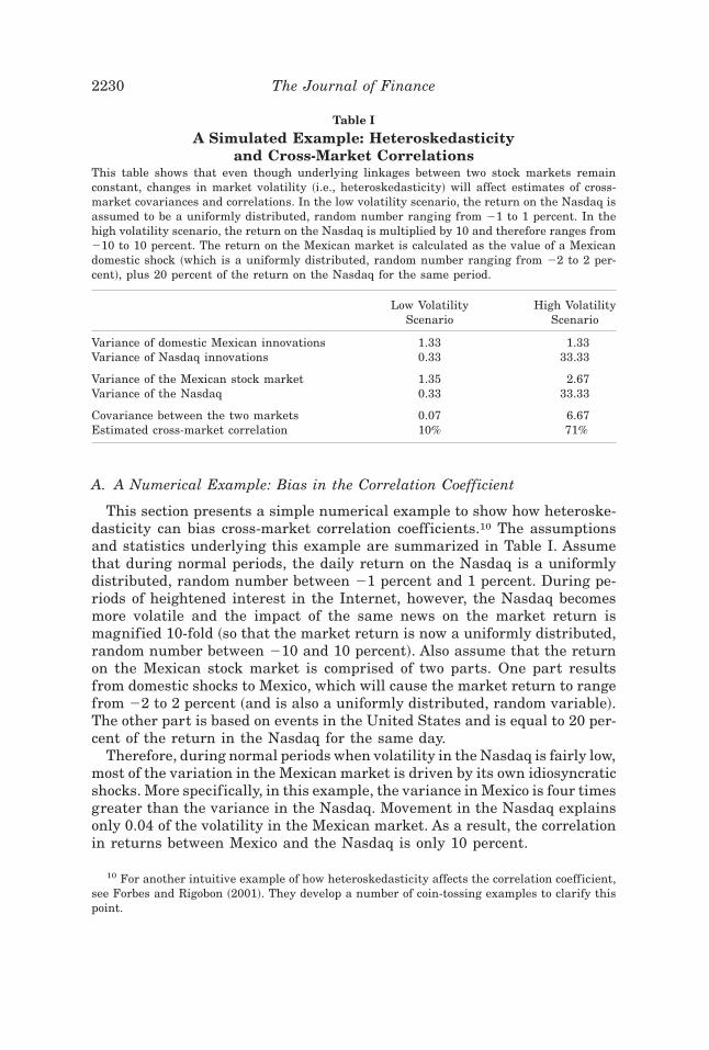
This section presents a simple numerical example to show how heteroske-dasticity can bias cross-market correlation coefficients.10 The assumptionsand statistics underlying this example are summarized in Table I. Assumethat during normal periods, the daily return on the Nasdaq is a uniformlydistributed, random number between 21 percent and 1 percent. During pe-riods of heightened interest in the Internet, however, the Nasdaq becomesmore volatile and the impact of the same news on the market return ismagnified 10-fold ~so that the market return is now a uniformly distributed,random number between 210 and 10 percent!. Also assume that the returnon the Mexican stock market is comprised of two parts. One part resultsfrom domestic shocks to Mexico, which will cause the market return to rangefrom 22 to 2 percent ~and is also a uniformly distributed, random variable!.The other part is based on events in the United States and is equal to 20 per-cent of the return in the Nasdaq for the same day.

Therefore, during normal periods when volatility in the Nasdaq is fairly low,most of the variation in the Mexican market is driven by its own idiosyncraticshocks. More specifically, in this example, the variance in Mexico is four timesgreater than the variance in the Nasdaq. Movement in the Nasdaq explainsonly 0.04 of the volatility in the Mexican market. As a result, the correlationin returns between Mexico and the Nasdaq is only 10 percent.

10 For another intuitive example of how heteroskedasticity affects the correlation coefficient,see Forbes and Rigobon ~2001!. They develop a number of coin-tossing examples to clarify thispoint.

Table I

A Simulated Example: Heteroskedasticityand Cross-Market Correlations

This table shows that even though underlying linkages between two stock markets remainconstant, changes in market volatility ~i.e., heteroskedasticity! will affect estimates of cross-market covariances and correlations. In the low volatility scenario, the return on the Nasdaq isassumed to be a uniformly distributed, random number ranging from 21 to 1 percent. In thehigh volatility scenario, the return on the Nasdaq is multiplied by 10 and therefore ranges from210 to 10 percent. The return on the Mexican market is calculated as the value of a Mexicandomestic shock ~which is a uniformly distributed, random number ranging from 22 to 2 per-cent!, plus 20 percent of the return on the Nasdaq for the same period.

Low VolatilityScenario

High VolatilityScenario

Variance of domestic Mexican innovations 1.33 1.33Variance of Nasdaq innovations 0.33 33.33

Variance of the Mexican stock market 1.35 2.67Variance of the Nasdaq 0.33 33.33

Covariance between the two markets 0.07 6.67Estimated cross-market correlation 10% 71%


On the other hand, during periods when the volatility of the Nasdaq in-creases, the proportion of the variation in the Mexican market driven bymovements in the Nasdaq increases significantly. More specifically, in theexample when shocks to the Nasdaq are uniformly distributed from 210 to10, the variance of these shocks is 25 times the variance of the domesticshocks to the Mexican market. As a result, movements in the Nasdaq ex-plain about 50 percent of the variance in the Mexican stock market, and thecorrelation between these two markets increases to over 70 percent.

This example clearly shows how an increase in market volatility can affectestimates of cross-market correlation coefficients.11 Even though the trans-mission mechanism from the Nasdaq to the Mexican market remains con-stant at 20 percent in both states of the world, estimates of the cross-marketcorrelation coefficient increase from 10 percent during the normal period to70 percent during the volatile period. Heteroskedasticity in returns ~i.e., theincreased volatility in the Nasdaq! will affect estimates of cross-market cor-relation coefficients, even when the underlying cross-market linkages re-main constant.

B. Proof of the Bias and a Proposed Correction

This section presents an informal proof of how heteroskedasticity biasesthe cross-market correlation coefficient. Appendix A presents a more formalproof.12 For simplicity, the following discussion focuses on the two-marketcase. Assume x and y are stochastic variables which represent stock marketreturns ~in different markets!, and these returns are related according to theequation:

yt 5 a 1 bxt 1 et , ~1!

where

E @et # 5 0, ~2!

E @et2# 5 c , ` ~3!

11 This simple example can be extended to its limiting values to emphasize the key point.The two markets continue to be linked through the same mechanisms: 20 percent of the Nasdaqreturn is transmitted to the Mexican market. Now assume that the variance of the Nasdaq fallsto zero. Then the covariance and correlation between the two stock markets will be zero. In theother extreme, assume that the variance of the Nasdaq goes to infinity ~or that the variancebecomes so large that innovations in the Mexican market are negligible by comparison!. Thenall the movement in the Mexican market is explained by movement in the Nasdaq, so that thecorrelation between the two markets increases to one. In each case, the true cross-marketlinkage remains constant ~at 0.20!, but the estimated correlation coefficient will move from0 to 1.

12 Both of these proofs build on Ronn ~1998!. Ronn, however, uses more restrictive assump-tions about the distribution of the residuals.


~where c is a constant!, and

E @xt et # 5 0. ~4!

Note that it is not necessary to make any further assumptions about thedistribution of the residuals. Divide the sample into two groups, so that thevariance of xt is lower in one group ~l ! and higher in the second group ~h!.In terms of our definition of contagion, the low-variance group is the periodof relative market stability and the high-variance group is the period ofmarket turmoil directly after the shock or crisis. In the context of the ex-ample with Mexico and the Nasdaq discussed above, the low-variance groupis the normal period and the high-variance group is the period of heightenedinterest in the Internet, so that a 5 0 and b 5 0.20 for both periods.

Next, since E@xt et # 5 0 by assumption in equation ~4!, OLS estimates of equa-tion ~1! are consistent for both groups and bh 5 b l. By construction, we knowthat sxx

h . sxxl , which, when combined with the standard definition of b:

bh 5sxy

h

sxxh 5

sxyl

sxxl 5 b l, ~5!

implies that sxyh . sxy

l . In other words, the cross-market covariance is higherin the second group. This increase in the cross-market covariance from thatin the first group is directly proportional to the increase in the variance of x.

Meanwhile, according to equation ~1!, the variance of y is

syy 5 b2sxx 1 see . ~6!

Since the variance of the residual is positive, the increase in the variance ofy across groups is less than proportional to the increase in the variance of x.In other words, since the variance of the residuals is assumed to remainconstant over the entire sample, this implies that the increase in the vari-ance of y across groups is less than proportional to the increase in the vari-ance of x. Therefore,

Ssxx

syyDh

. Ssxx

syyDl

. ~7!

Finally, substitute equation ~5! into the standard definition of the correla-tion coefficient:

r 5sxy

sx sy5 b

sx

sy, ~8!

and, when combined with equation ~7!, this implies that rh . r l.


As a result, the estimated correlation between x and y increases when thevariance of x increases—even if the true relationship ~b! between x and y isconstant. Therefore, tests for a change in cross-market transmission mech-anisms based on the correlation coefficient can be misleading. Estimates ofthe correlation coefficient are biased and conditional on the variance of x.

The formal proof presented in Appendix A shows that it is possible toquantify the extent of this bias. More specifically, if we continue to assumethe absence of endogeneity ~equation ~4!! and omitted variables ~equation~2!!, the conditional correlation can be written as

r* 5 r! 1 1 d

1 1 dr2 , ~9!

where r* is the conditional correlation coefficient, r is the unconditionalcorrelation coefficient, and d is the relative increase in the variance of x:

d [sxx

h

sxxl 2 1. ~10!

Equation ~9! clearly shows that the estimated correlation coefficient isincreasing in d. Therefore, during periods of high volatility in market x, theestimated correlation ~i.e., the conditional correlation! between markets yand x will be greater than the unconditional correlation. In other words,even if the unconditional correlation coefficient remains constant during astable period and volatile period, the conditional correlation coefficient willbe greater during the more volatile period.

This result has direct implications for tests for contagion based on cross-market correlation coefficients. Markets tend to be more volatile after ashock or crisis. Therefore, the conditional correlation coefficient will tend toincrease after a crisis, even if the unconditional correlation coefficient ~theunderlying cross-market relationship! is the same as during more stableperiods. In other words, heteroskedasticity in market returns can cause es-timates of cross-market correlation coefficients to be biased upward after acrisis. Formal tests for contagion could find a significant increase in theestimated, conditional correlation coefficients after a crisis. Without adjust-ing for the bias, however, it is impossible to deduce if this increase in theconditional correlation represents an increase in the unconditional correla-tion or simply an increase in market volatility. According to our definition,only an increase in the unconditional correlation coefficient would constitutecontagion.

Under the assumptions discussed above, it is straightforward to adjust forthis bias. Simple manipulation of equations ~9! and ~10! to solve for theunconditional correlation coefficient yields

r 5r*

!1 1 d@1 2 ~ r* !2 #. ~11!


One potential problem with this adjustment for heteroskedasticity is thatit assumes there are no omitted variables or endogeneity between markets~written as equations ~2! and ~4!!. In other words, the proof of this bias andthe adjustment is only valid if there are no exogenous global shocks and nofeedback from stock market y to x. These assumptions are clearly a simpli-fication, but there does not currently exist any procedure that can adjust thecorrelation coefficient without making these two assumptions. Appendix Banalyzes the impact of relaxing these two assumptions. This appendix showsthat the correlation coefficient is still biased in the presence of heteroske-dasticity and omitted variables or endogeneity. It also shows that withoutmaking additional assumptions, it is impossible to estimate the extent ofthis bias and, therefore, impossible to make any sort of simple adjustment tocalculate the unconditional correlation coefficient.

On a more positive note, however, Appendix B also shows that the adjust-ment in equation ~11! is a relatively good approximation of the unconditionalcorrelation coefficient if the change in the variance is large and it is possibleto identify the country where the shock originates. The intuition behind thesefindings is based on what the simultaneous-equations literature calls near iden-tification. More specifically, assume that there are two countries whose re-turns are simultaneously determined and both affected by the same aggregateshock as well as their own idiosyncratic shocks. If the idiosyncratic shock af-fecting one country is much larger than the aggregate shock, then the adjust-ment to the correlation coefficient proposed in equation ~11! is fairly accurate.

In the empirical implementation below, we ascertain that these criteriafor near identification are valid when deciding which pairs of correlations tocalculate and test for contagion. The three criteria are: a major shift inmarket volatility, clear identification of which country generates this shift involatility, and inclusion of the relevant country as one market in the esti-mated correlation. The data suggests that these criteria are satisfied duringthe crisis periods investigated in this paper. During the three relevant pe-riods, the variance of returns in the crisis countries increased by over 10times, and the source of the shock is clear ~the United States in 1987, Mexicoin 1994, and Hong Kong in October, 1997!. We only test for contagion fromthe country where the shock originates to other countries in the sample. Forexample, during December 1994, there was a large increase in market vol-atility caused mainly by events in Mexico. Therefore, it is only valid to usethis framework and the adjustment in equation ~11! to analyze cross-marketcorrelations between Mexico and each of the other countries in the sampleduring this period. ~It is not valid to use this framework, for example, to testfor contagion from Chile to Argentina during this period.!

C. A Graphical Example: The Bias in Tests for Contagion

To clarify the intuition behind this bias in the cross-market correlationcoefficient and its potential importance in tests for contagion, Figure 4 graphsthe correlation in stock market returns between Hong Kong and the Philip-


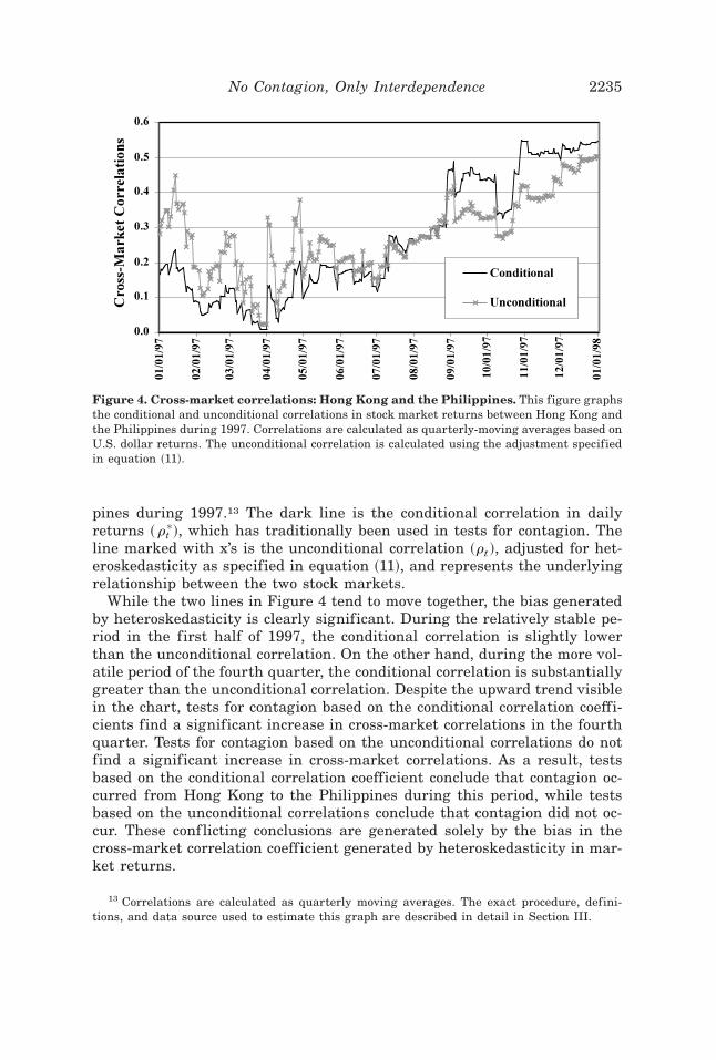
pines during 1997.13 The dark line is the conditional correlation in dailyreturns ~ rt

*!, which has traditionally been used in tests for contagion. Theline marked with x’s is the unconditional correlation ~rt !, adjusted for het-eroskedasticity as specified in equation ~11!, and represents the underlyingrelationship between the two stock markets.

While the two lines in Figure 4 tend to move together, the bias generatedby heteroskedasticity is clearly significant. During the relatively stable pe-riod in the first half of 1997, the conditional correlation is slightly lowerthan the unconditional correlation. On the other hand, during the more vol-atile period of the fourth quarter, the conditional correlation is substantiallygreater than the unconditional correlation. Despite the upward trend visiblein the chart, tests for contagion based on the conditional correlation coeffi-cients find a significant increase in cross-market correlations in the fourthquarter. Tests for contagion based on the unconditional correlations do notfind a significant increase in cross-market correlations. As a result, testsbased on the conditional correlation coefficient conclude that contagion oc-curred from Hong Kong to the Philippines during this period, while testsbased on the unconditional correlations conclude that contagion did not oc-cur. These conf licting conclusions are generated solely by the bias in thecross-market correlation coefficient generated by heteroskedasticity in mar-ket returns.

13 Correlations are calculated as quarterly moving averages. The exact procedure, defini-tions, and data source used to estimate this graph are described in detail in Section III.

Figure 4. Cross-market correlations: Hong Kong and the Philippines. This figure graphsthe conditional and unconditional correlations in stock market returns between Hong Kong andthe Philippines during 1997. Correlations are calculated as quarterly-moving averages based onU.S. dollar returns. The unconditional correlation is calculated using the adjustment specifiedin equation ~11!.


III. The Base Model and the Data

Before formally analyzing how heteroskedasticity biases tests for conta-gion during recent financial crises, this section brief ly discusses our modelspecification and data set. To adjust for the fact that stock markets are openduring different hours, as well as to control for serial correlation in stockreturns and any exogenous global shocks, we utilize a VAR framework toestimate cross-market correlations. More specifically, the base specifica-tion is:

Xt 5 f~L!Xt 1 F~L! It 1 ht ~12!

Xt [ $xtC , xt

j% ' ~13!

It [ $itC , it

US , itj% ', ~14!

where xtC is the stock market return in the crisis country; xt

j is the stockmarket return in another market j; Xt is a transposed vector of returns inthe same two stock markets; f~L! and F~L! are vectors of lags; it

C , itUS , and

itj are short-term interest rates for the crisis country, the United States, and

country j, respectively; and ht is a vector of reduced-form disturbances. Foreach series of tests, we first use the VAR model in equations ~12! through~14! to estimate the variance–covariance matrices for each pair of countriesduring the stable period, turmoil period, and full period. Then we use theestimated variance–covariance matrices to calculate the cross-market corre-lation coefficients ~and their asymptotic distributions! for each set of coun-tries and periods.

Stock market returns are calculated as rolling-average, two-day returnsbased on each country ’s aggregate stock market index.14 We utilize averagetwo-day returns to control for the fact that markets in different countriesare not open during the same hours. We calculate returns based on U.S.dollars as well as local currency, but focus on U.S. dollar returns since thesewere most frequently used in past work on contagion. We utilize five lags forf~L! and F~L! in order to control for serial correlation and any within-weekvariation in trading patterns. We include interest rates in order to controlfor any aggregate shocks and0or monetary policy coordination.15 All of thedata is from Datastream. An extensive set of sensitivity tests ~many of whichare reported below!, show that changing the model specification has no sig-nificant impact on results. For example, using daily or weekly returns, localcurrency returns, greater or fewer lags, and0or varying the interest ratecontrols does not change our central findings. Moreover, the sensitivity analy-

14 Daily returns are also adjusted for weekends and holidays.15 Although interest rates are an imperfect measure of aggregate shocks, they are a good

proxy for global shifts in real economic variables and0or policies that affect stock marketperformance.


sis also shows that focusing only on the cross-market correlation coefficient—with daily returns, no lags, and no interest rate controls—actually strengthensour central results.

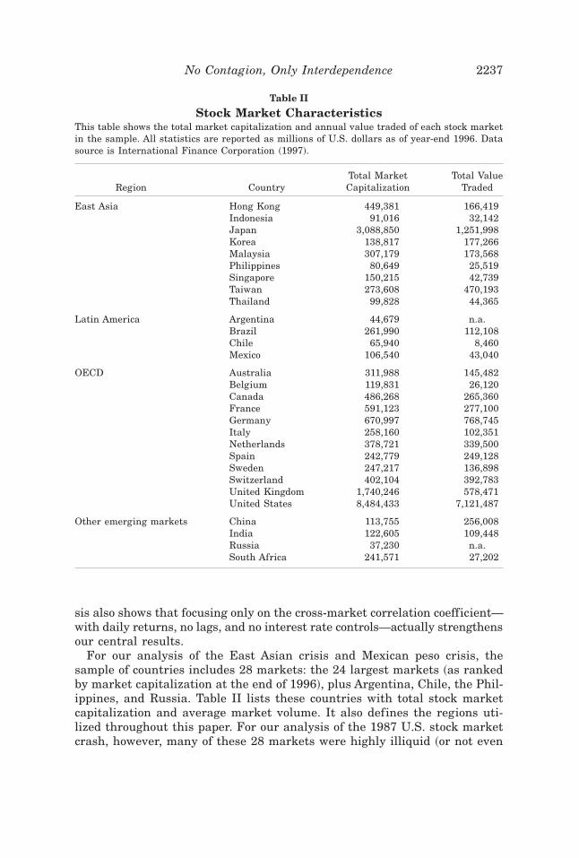
For our analysis of the East Asian crisis and Mexican peso crisis, thesample of countries includes 28 markets: the 24 largest markets ~as rankedby market capitalization at the end of 1996!, plus Argentina, Chile, the Phil-ippines, and Russia. Table II lists these countries with total stock marketcapitalization and average market volume. It also defines the regions uti-lized throughout this paper. For our analysis of the 1987 U.S. stock marketcrash, however, many of these 28 markets were highly illiquid ~or not even

Table II

Stock Market CharacteristicsThis table shows the total market capitalization and annual value traded of each stock marketin the sample. All statistics are reported as millions of U.S. dollars as of year-end 1996. Datasource is International Finance Corporation ~1997!.

Region CountryTotal MarketCapitalization

Total ValueTraded

East Asia Hong Kong 449,381 166,419Indonesia 91,016 32,142Japan 3,088,850 1,251,998Korea 138,817 177,266Malaysia 307,179 173,568Philippines 80,649 25,519Singapore 150,215 42,739Taiwan 273,608 470,193Thailand 99,828 44,365

Latin America Argentina 44,679 n.a.Brazil 261,990 112,108Chile 65,940 8,460Mexico 106,540 43,040

OECD Australia 311,988 145,482Belgium 119,831 26,120Canada 486,268 265,360France 591,123 277,100Germany 670,997 768,745Italy 258,160 102,351Netherlands 378,721 339,500Spain 242,779 249,128Sweden 247,217 136,898Switzerland 402,104 392,783United Kingdom 1,740,246 578,471United States 8,484,433 7,121,487

Other emerging markets China 113,755 256,008India 122,605 109,448Russia 37,230 n.a.South Africa 241,571 27,202


in existence!. Therefore, during this earlier period we only include the 10largest markets.

IV. Contagion from Hong Kong during the 1997 East Asian Crisis

As our first empirical analysis of how heteroskedasticity biases tests forcontagion based on the correlation coefficient, we consider the East Asiancrisis of 1997. One difficulty in testing for contagion during this period isthat no single event acts as a clear catalyst behind this turmoil. For exam-ple, the Thai market declined sharply in June, the Indonesian market fell inAugust, and the Hong Kong market crashed in mid-October. A review ofAmerican and British newspapers and periodicals during this period, how-ever, shows an interesting pattern. The press in these countries paid littleattention to the earlier movements in the Thai and Indonesian markets un-til the sharp decline in the Hong Kong market in mid-October. After this,events in Asia became headline news, and an avid discussion quickly beganon the East Asian “crisis” and the possibility of “contagion” to the rest of theworld.

Therefore, for our base analysis, we focus on tests for contagion from HongKong to the rest of the world during the volatile period directly after theHong Kong crash. It is obviously possible that contagion occurred duringother periods of time, or from the combined impact of turmoil in a group ofEast Asian markets instead of in a single country. We test for these varioustypes of contagion in the sensitivity analysis and show that using thesedifferent contagion sources has no significant impact on key results.16 Usingthe October decline in the Hong Kong market as the base for our contagiontests, we define our “turmoil” period as the month starting on October 17,1997 ~the start of this visible Hong Kong crash!. We define the “stable” pe-riod as January 1, 1996, to the start of the turmoil period.17

Then we estimate the VAR model specified in equations ~12! through ~14!with Hong Kong as the crisis country ~c!. Using the variance–covarianceestimates from this model, we calculate the cross-market correlation coeffi-cients between Hong Kong and each of the other countries in the sampleduring the stable period, turmoil period, and full period. Then we use thesecoefficients to perform the standard test for contagion described at the startof Section I. These are based on the conditional correlation coefficients andare not adjusted for heteroskedasticity. Finally, we use t-tests to evaluate if

16 Many papers date the start of the Asian crisis as the Thai devaluation in July 1997. Thesensitivity analysis shows, however, that there were few cases of contagion after the Thai de-valuation ~based on the conditional correlation coefficients!, and since markets were less vol-atile during this earlier period, the bias in tests for contagion is less problematic. Therefore, forthe purpose of this paper, the Hong Kong crisis provides a cleaner example of how heteroske-dasticity can bias tests for contagion.

17 A sensitivity analysis shows that period definition does not affect the central results. Wedo not utilize a longer length of time for the stable period in our base estimates due to the factthat any structural change in markets over this period would invalidate the tests for contagion.


there is a significant increase in any of these correlation coefficients duringthe turmoil period.18 If r is the correlation during the full period and rt

h isthe correlation during the turmoil ~high volatility! period, the test hypoth-eses are

H0 : r . rth

H1 : r # rth .

~15!

The estimated, conditional correlation coefficients for the stable, turmoil,and full period are shown in Table III. The critical value for the t-test at thefive percent level is 1.65, so any test statistic greater than this critical valueindicates contagion ~C!, while any statistic less than or equal to this valueindicates no contagion ~N!. Test statistics and results are reported on theright of the table.

Several patterns are immediately apparent. First, cross-market correla-tions during the relatively stable period are not surprising. Hong Kong ishighly correlated with Australia and many of the East Asian economies, andmuch less correlated with Latin American markets. Second, cross-marketcorrelations between Hong Kong and most of the other countries in the sam-ple increase during the turmoil period. This is a prerequisite for contagion tooccur. This change is especially notable in many of the OECD markets, wherethe average correlation with Hong Kong increases from 0.22 during the sta-ble period to 0.68 during the turmoil period. In one extreme example, thecorrelation between Hong Kong and Belgium increases from 0.14 in the sta-ble period to 0.71 in the turmoil period. Third, the t-tests indicate a signif-icant increase in this conditional correlation coefficient during the turmoilperiod for 15 countries. According to the standard interpretation in this lit-erature, this implies that contagion occurred from the October crash of theHong Kong market to Australia, Belgium, Chile, France, Germany, Indone-sia, Italy, Korea, the Netherlands, the Philippines, Russia, South Africa, Spain,Sweden, and Switzerland.

As discussed above, however, these tests for contagion may be inaccuratedue to the bias in the correlation coefficient resulting from heteroskedastic-ity. The estimated increases in the conditional correlation coefficient couldref lect either an increase in cross-market linkages and0or increased marketvolatility. To test how any bias in the correlation coefficient affects our testsfor contagion, we repeat this analysis but use the correction in equation ~11!to adjust for this bias. In other words, we repeat the above analysis usingthe unconditional instead of the conditional correlation coefficients. Uncon-ditional correlation coefficients and test results are shown in Table IV.

18 We have also experimented with a number of other tests, such as two-sided tests and0orcomparing the correlation coefficient during the turmoil period with that during the stableperiod ~instead of the full period!. In each case, test specification has no significant impact onresults.


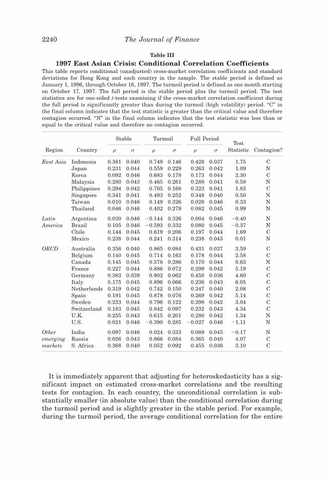
It is immediately apparent that adjusting for heteroskedasticity has a sig-nificant impact on estimated cross-market correlations and the resultingtests for contagion. In each country, the unconditional correlation is sub-stantially smaller ~in absolute value! than the conditional correlation duringthe turmoil period and is slightly greater in the stable period. For example,during the turmoil period, the average conditional correlation for the entire

Table III

1997 East Asian Crisis: Conditional Correlation CoefficientsThis table reports conditional ~unadjusted! cross-market correlation coefficients and standarddeviations for Hong Kong and each country in the sample. The stable period is defined asJanuary 1, 1996, through October 16, 1997. The turmoil period is defined as one month startingon October 17, 1997. The full period is the stable period plus the turmoil period. The teststatistics are for one-sided t-tests examining if the cross-market correlation coefficient duringthe full period is significantly greater than during the turmoil ~high volatility! period. “C” inthe final column indicates that the test statistic is greater than the critical value and thereforecontagion occurred. “N” in the final column indicates that the test statistic was less than orequal to the critical value and therefore no contagion occurred.

Stable Turmoil Full Period

Region Country r s r s r sTest

Statistic Contagion?

East Asia Indonesia 0.381 0.040 0.749 0.146 0.428 0.037 1.75 CJapan 0.231 0.044 0.559 0.229 0.263 0.042 1.09 NKorea 0.092 0.046 0.683 0.178 0.173 0.044 2.30 CMalaysia 0.280 0.043 0.465 0.261 0.288 0.041 0.58 NPhilippines 0.294 0.042 0.705 0.168 0.323 0.041 1.83 CSingapore 0.341 0.041 0.493 0.252 0.348 0.040 0.50 NTaiwan 0.010 0.046 0.149 0.326 0.028 0.046 0.33 NThailand 0.046 0.046 0.402 0.279 0.082 0.045 0.99 N

Latin Argentina 0.030 0.046 20.144 0.326 0.004 0.046 20.40 NAmerica Brazil 0.105 0.046 20.593 0.332 0.080 0.045 20.37 N

Chile 0.144 0.045 0.619 0.206 0.197 0.044 1.69 CMexico 0.238 0.044 0.241 0.314 0.238 0.043 0.01 N

OECD Australia 0.356 0.040 0.865 0.084 0.431 0.037 3.59 CBelgium 0.140 0.045 0.714 0.163 0.178 0.044 2.58 CCanada 0.145 0.045 0.378 0.286 0.170 0.044 0.63 NFrance 0.227 0.044 0.886 0.072 0.299 0.042 5.19 CGermany 0.383 0.039 0.902 0.062 0.450 0.036 4.60 CItaly 0.175 0.045 0.896 0.066 0.236 0.043 6.05 CNetherlands 0.319 0.042 0.742 0.150 0.347 0.040 2.08 CSpain 0.191 0.045 0.878 0.076 0.269 0.042 5.14 CSweden 0.233 0.044 0.796 0.122 0.298 0.042 3.04 CSwitzerland 0.183 0.045 0.842 0.097 0.232 0.043 4.34 CU.K. 0.255 0.043 0.615 0.201 0.280 0.042 1.34 NU.S. 0.021 0.046 20.390 0.285 20.027 0.046 21.11 N

Other India 0.097 0.046 0.024 0.333 0.089 0.045 20.17 Nemerging Russia 0.026 0.043 0.866 0.084 0.365 0.040 4.07 Cmarkets S. Africa 0.368 0.040 0.052 0.092 0.455 0.036 3.10 C


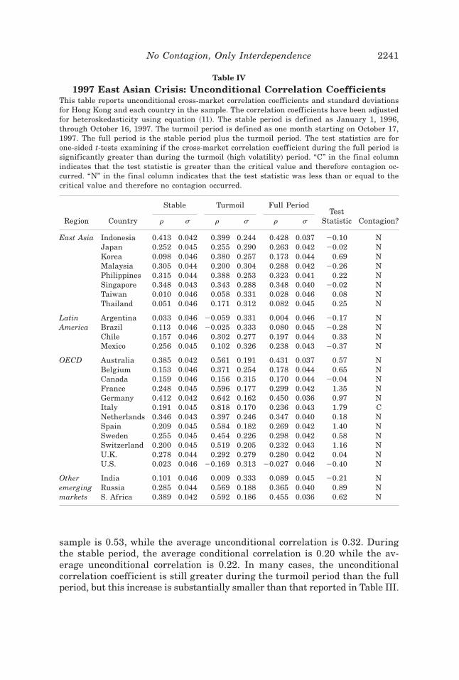
sample is 0.53, while the average unconditional correlation is 0.32. Duringthe stable period, the average conditional correlation is 0.20 while the av-erage unconditional correlation is 0.22. In many cases, the unconditionalcorrelation coefficient is still greater during the turmoil period than the fullperiod, but this increase is substantially smaller than that reported in Table III.

Table IV

1997 East Asian Crisis: Unconditional Correlation CoefficientsThis table reports unconditional cross-market correlation coefficients and standard deviationsfor Hong Kong and each country in the sample. The correlation coefficients have been adjustedfor heteroskedasticity using equation ~11!. The stable period is defined as January 1, 1996,through October 16, 1997. The turmoil period is defined as one month starting on October 17,1997. The full period is the stable period plus the turmoil period. The test statistics are forone-sided t-tests examining if the cross-market correlation coefficient during the full period issignificantly greater than during the turmoil ~high volatility! period. “C” in the final columnindicates that the test statistic is greater than the critical value and therefore contagion oc-curred. “N” in the final column indicates that the test statistic was less than or equal to thecritical value and therefore no contagion occurred.




East Asia Indonesia 0.413 0.042 0.399 0.244 0.428 0.037 20.10 NJapan 0.252 0.045 0.255 0.290 0.263 0.042 20.02 NKorea 0.098 0.046 0.380 0.257 0.173 0.044 0.69 NMalaysia 0.305 0.044 0.200 0.304 0.288 0.042 20.26 NPhilippines 0.315 0.044 0.388 0.253 0.323 0.041 0.22 NSingapore 0.348 0.043 0.343 0.288 0.348 0.040 20.02 NTaiwan 0.010 0.046 0.058 0.331 0.028 0.046 0.08 NThailand 0.051 0.046 0.171 0.312 0.082 0.045 0.25 N


Chile 0.157 0.046 0.302 0.277 0.197 0.044 0.33 NMexico 0.256 0.045 0.102 0.326 0.238 0.043 20.37 N

OECD Australia 0.385 0.042 0.561 0.191 0.431 0.037 0.57 NBelgium 0.153 0.046 0.371 0.254 0.178 0.044 0.65 NCanada 0.159 0.046 0.156 0.315 0.170 0.044 20.04 NFrance 0.248 0.045 0.596 0.177 0.299 0.042 1.35 NGermany 0.412 0.042 0.642 0.162 0.450 0.036 0.97 NItaly 0.191 0.045 0.818 0.170 0.236 0.043 1.79 CNetherlands 0.346 0.043 0.397 0.246 0.347 0.040 0.18 NSpain 0.209 0.045 0.584 0.182 0.269 0.042 1.40 NSweden 0.255 0.045 0.454 0.226 0.298 0.042 0.58 NSwitzerland 0.200 0.045 0.519 0.205 0.232 0.043 1.16 NU.K. 0.278 0.044 0.292 0.279 0.280 0.042 0.04 NU.S. 0.023 0.046 20.169 0.313 20.027 0.046 20.40 N

Other India 0.101 0.046 0.009 0.333 0.089 0.045 20.21 Nemerging Russia 0.285 0.044 0.569 0.188 0.365 0.040 0.89 Nmarkets S. Africa 0.389 0.042 0.592 0.186 0.455 0.036 0.62 N


For example, the conditional correlation between Hong Kong and the Neth-erlands jumps from 0.35 during the full period to 0.74 during the turmoilperiod, while the unconditional correlation only increases from 0.35 to 0.40.Moreover, when tests for contagion are performed on these unconditionalcorrelations, only one coefficient ~for Italy! increases significantly duringthe turmoil period. In other words, according to this testing methodology,there is only evidence of contagion from the Hong Kong crash to one othercountry in the sample ~versus 15 cases of contagion when tests are based onthe conditional correlations!.

Moreover, these results highlight exactly how this testing methodologydefines contagion. Many stock markets are highly correlated with Hong Kong’smarket during this volatile period in October and November of 1997. Forexample, during this period, the unconditional correlation between HongKong and Australia is 0.56 and that between Hong Kong and the Philippinesis 0.39. These high cross-market correlations do not qualify as contagion,however, because these markets are correlated to a similar high degree dur-ing more stable periods. These stock markets are highly interdependent inall states of the world. Therefore, according to the assumptions and simpletests performed above, this interdependence does not change significantlyduring October and November of 1997.

A. Sensitivity Tests

Since this adjustment to the correlation coefficient has such a significantimpact on our analysis, we perform an extensive series of sensitivity tests.In the following section, we test for the impact of modifying the period def-initions, the source of contagion, the frequency of returns, the lag structure,the interest rate controls, and the currency denomination. In each case ~aswell as others not reported below!, the central results do not change. Testsbased on the conditional correlation coefficients find some evidence of con-tagion, while tests based on the unconditional coefficients ~adjusted accord-ing to equation ~11!! find virtually no evidence of contagion. Due to therepetition of these tests, we only report a selection of summary results foreach analysis.19

As a first set of robustness tests, we modify definitions for the stable andturmoil periods. In the base analysis, we define the stable period as Janu-ary 1, 1996, through October 16, 1997, and the turmoil period as the monthstarting on October 17, 1997. We begin by defining the turmoil period asstarting at an earlier date, such as on June 1, 1997 ~when the Thai marketfirst dropped! or on August 7, 1997 ~when the Indonesian and Thai marketsbegan their simultaneous decline!. Next we extend the turmoil period to endon March 1, 1998. Then we extend the length of the stable period by definingit to begin on January 1, 1993, or January 1, 1995. A selection of these

19 Complete results are available from the authors.


results is reported near the top of Table V. The base case is reported in bolditalics in the first row of the table.

For a second set of sensitivity tests, we examine how altering the definedsource of contagion can impact results. As discussed above, one difficulty intesting for contagion during the East Asian crisis is that there is no singleevent acting as a clear catalyst driving this turmoil. We begin by testing forcontagion from single East Asian markets ~other than Hong Kong! after asignificant downturn in those markets: from Thailand after its June decline;from Thailand or Indonesia after their August losses; or from Korea for thetwo-months after its crash that started in late October. Next, since conta-gion may occur from the combined impact of movements in several EastAsian markets, we construct several East Asian indices.20 We test for con-tagion from Thailand and Indonesia after the August crashes in both ofthese markets; from Hong Kong and Korea during several tumultuous pe-riods in these markets; and from Hong Kong, Indonesia, Korea, Malaysia,and Thailand ~a five-country index! during several different periods. Sum-mary results for a selection of these tests are reported in the middle ofTable V.

As a third series of robustness tests, we adjust the frequency of returnsand0or lag structure. In our base analysis, we focus on rolling-average, two-day returns in order to control for the fact that different stock markets areopen during different hours. We also include five lags of the cross-marketcorrelations ~Xt ! and the vector of interest rates ~It !. We repeat this analysisusing daily returns and weekly returns. We also combine each of these re-turn calculations with zero, one, or five lags ~as possible! of Xt and It .21 Aselection of results is reported near the bottom of Table V.

For a final series of sensitivity tests, we vary the interest rate controlsand currency denomination. First, we include no interest rates in the modelor only include interest rates in the United States or the crisis country. Thenwe repeat the analysis with local-currency returns with a variety of lag andreturn structures. A sample of these results is reported at the bottom ofTable V. It is worth noting that the results reported in the last row of thetable—with daily returns, no lags, and no interest rate controls—is a test forcontagion in the simple theoretical model ~developed in Section II! beforeadding the additional controls and extensions in Section III.

This series of sensitivity tests reported in Table V suggests that a widerange of modifications to our base model do not affect the central results.When tests for a significant change in cross-market relationships are basedon the conditional correlation coefficients, there is evidence of contagion in

20 To calculate each index, we weight each country by total market capitalization at the endof 1996, as reported in Table II.

21 Note that in each case, estimates are only consistent if there are at least as many lags~minus one! as the number of days averaged to calculate the returns. Lags are required becausewe utilize a moving average to measure returns. Therefore, by construction, observations attime t are correlated with those at t 2 1, t 2 2, and so forth. Also note that we do not use morethan five lags due to the short length of the turmoil period.


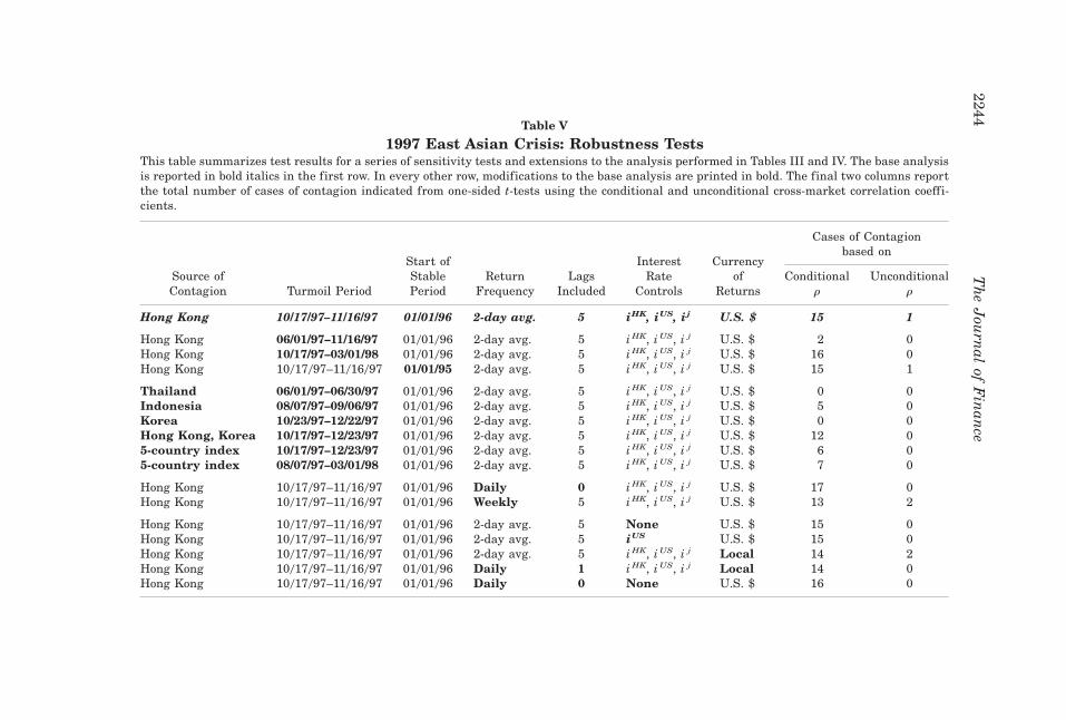
Table V

1997 East Asian Crisis: Robustness TestsThis table summarizes test results for a series of sensitivity tests and extensions to the analysis performed in Tables III and IV. The base analysisis reported in bold italics in the first row. In every other row, modifications to the base analysis are printed in bold. The final two columns reportthe total number of cases of contagion indicated from one-sided t-tests using the conditional and unconditional cross-market correlation coeffi-cients.

Cases of Contagionbased on

Source ofContagion Turmoil Period

Start ofStablePeriod

ReturnFrequency

LagsIncluded

InterestRate

Controls

Currencyof

ReturnsConditional

rUnconditional

r

Hong Kong 10/17/97–11/16/97 01/01/96 2-day avg. 5 iHK, iUS, i j U.S. $ 15 1

Hong Kong 06/01/97–11/16/97 01001096 2-day avg. 5 i HK, i US, i j U.S. $ 2 0Hong Kong 10/17/97–03/01/98 01001096 2-day avg. 5 i HK, i US, i j U.S. $ 16 0Hong Kong 10017097–11016097 01/01/95 2-day avg. 5 i HK, i US, i j U.S. $ 15 1

Thailand 06/01/97–06/30/97 01001096 2-day avg. 5 i HK, i US, i j U.S. $ 0 0Indonesia 08/07/97–09/06/97 01001096 2-day avg. 5 i HK, i US, i j U.S. $ 5 0Korea 10/23/97–12/22/97 01001096 2-day avg. 5 i HK, i US, i j U.S. $ 0 0Hong Kong, Korea 10/17/97–12/23/97 01001096 2-day avg. 5 i HK, i US, i j U.S. $ 12 05-country index 10/17/97–12/23/97 01001096 2-day avg. 5 i HK, i US, i j U.S. $ 6 05-country index 08/07/97–03/01/98 01001096 2-day avg. 5 i HK, i US, i j U.S. $ 7 0

Hong Kong 10017097–11016097 01001096 Daily 0 i HK, i US, i j U.S. $ 17 0Hong Kong 10017097–11016097 01001096 Weekly 5 i HK, i US, i j U.S. $ 13 2

Hong Kong 10017097–11016097 01001096 2-day avg. 5 None U.S. $ 15 0Hong Kong 10017097–11016097 01001096 2-day avg. 5 iUS U.S. $ 15 0Hong Kong 10017097–11016097 01001096 2-day avg. 5 i HK, i US, i j Local 14 2Hong Kong 10017097–11016097 01001096 Daily 1 i HK, i US, i j Local 14 0Hong Kong 10017097–11016097 01001096 Daily 0 None U.S. $ 16 0

2244T

he

Jou

rnal

ofF

inan

ce

about half the sample ~with the number of cases highly dependent on thespecification estimated!. When tests are based on the unconditional corre-lation coefficients, there is virtually no evidence of a significant increase incross-market linkages.

V. Contagion during the 1994 Mexican Peso Crisis

As our second analysis of how bias in the correlation coefficient can affecttests for contagion, we compare cross-market correlations before and afterthe Mexican peso crisis of 1994. In December 1994, the Mexican governmentsuffered a balance of payments crisis, leading to a devaluation of the pesoand a precipitous decline in the Mexican stock market. This crisis generatedfears that contagion could quickly lead to crises in other emerging marketsand especially in the rest of Latin America. This analysis is more straight-forward than that of the East Asian crisis due to the existence of one clearcatalyst driving any contagion.

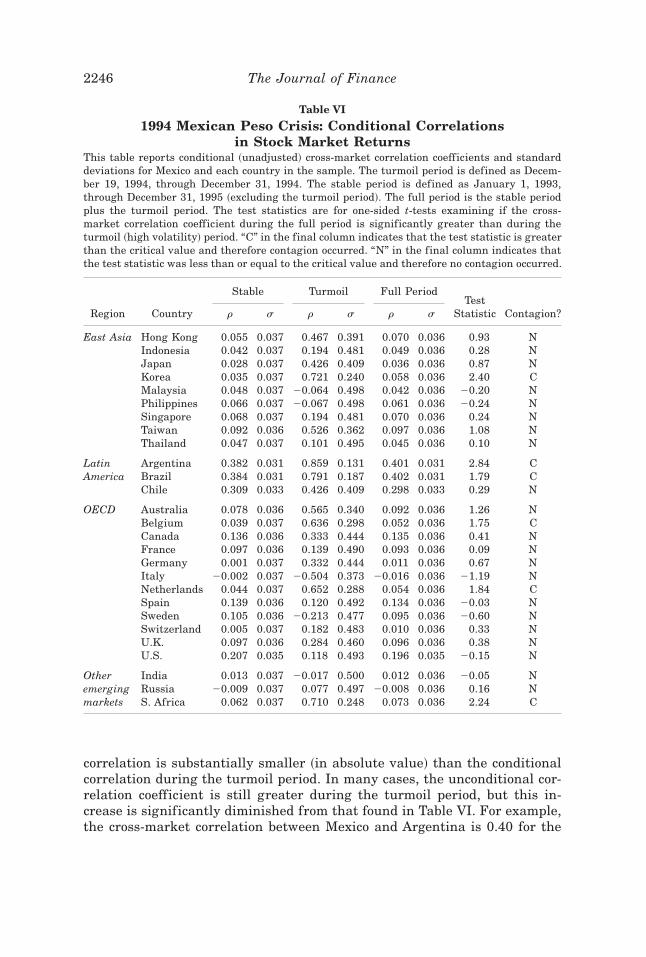
For our base test, we define the turmoil period in the Mexican market aslasting from December 19, 1994 ~the day the exchange rate regime was aban-doned! through December 31, 1994. We define the entire period as Janu-ary 1, 1993 through December 31, 1995 ~with the stable period including alldays except the turmoil period!. Next, we estimate the same system of equa-tions ~12! through ~14! with Mexico as the crisis country ~c!. We repeat thestandard test for stock market contagion: test for a significant increase incross-market correlations during the turmoil period. Estimates of the con-ditional correlation coefficients ~which have not been adjusted for hetero-skedasticity! and test results are shown in Table VI.

These conditional correlation coefficients show many patterns similar tothe East Asian case. First, during the relatively stable period, the Mexicanmarket tends to be more highly correlated with markets in the same region.Second, cross-market correlations between Mexico and most countries in thesample increase during the turmoil period. This is a prerequisite for conta-gion to occur. Many developed countries that are not highly correlated withMexico during the stable period become highly correlated during the turmoilperiod. Third, the t-tests indicate that there is a significant increase ~at thefive percent level! in the correlation coefficient during the turmoil period forsix countries. According to the interpretation used in previous empirical work,this indicates that contagion occurred from the Mexican stock market inDecember 1994 to Argentina, Belgium, Brazil, Korea, the Netherlands, andSouth Africa.

As discovered above, however, this evidence of contagion could result fromheteroskedasticity biasing estimates of cross-market correlations. Therefore,we repeat these tests using equation ~11! to adjust for this bias ~again underthe assumptions of no omitted variables or endogeneity!. Estimated uncon-ditional correlation coefficients and test results are shown in Table VII. Onceagain, this adjustment has a significant impact on estimated correlationsand the resulting tests for contagion. In each country, the unconditional


correlation is substantially smaller ~in absolute value! than the conditionalcorrelation during the turmoil period. In many cases, the unconditional cor-relation coefficient is still greater during the turmoil period, but this in-crease is significantly diminished from that found in Table VI. For example,the cross-market correlation between Mexico and Argentina is 0.40 for the

Table VI

1994 Mexican Peso Crisis: Conditional Correlationsin Stock Market Returns

This table reports conditional ~unadjusted! cross-market correlation coefficients and standarddeviations for Mexico and each country in the sample. The turmoil period is defined as Decem-ber 19, 1994, through December 31, 1994. The stable period is defined as January 1, 1993,through December 31, 1995 ~excluding the turmoil period!. The full period is the stable periodplus the turmoil period. The test statistics are for one-sided t-tests examining if the cross-market correlation coefficient during the full period is significantly greater than during theturmoil ~high volatility! period. “C” in the final column indicates that the test statistic is greaterthan the critical value and therefore contagion occurred. “N” in the final column indicates thatthe test statistic was less than or equal to the critical value and therefore no contagion occurred.




East Asia Hong Kong 0.055 0.037 0.467 0.391 0.070 0.036 0.93 NIndonesia 0.042 0.037 0.194 0.481 0.049 0.036 0.28 NJapan 0.028 0.037 0.426 0.409 0.036 0.036 0.87 NKorea 0.035 0.037 0.721 0.240 0.058 0.036 2.40 CMalaysia 0.048 0.037 20.064 0.498 0.042 0.036 20.20 NPhilippines 0.066 0.037 20.067 0.498 0.061 0.036 20.24 NSingapore 0.068 0.037 0.194 0.481 0.070 0.036 0.24 NTaiwan 0.092 0.036 0.526 0.362 0.097 0.036 1.08 NThailand 0.047 0.037 0.101 0.495 0.045 0.036 0.10 N

Latin Argentina 0.382 0.031 0.859 0.131 0.401 0.031 2.84 CAmerica Brazil 0.384 0.031 0.791 0.187 0.402 0.031 1.79 C

Chile 0.309 0.033 0.426 0.409 0.298 0.033 0.29 N

OECD Australia 0.078 0.036 0.565 0.340 0.092 0.036 1.26 NBelgium 0.039 0.037 0.636 0.298 0.052 0.036 1.75 CCanada 0.136 0.036 0.333 0.444 0.135 0.036 0.41 NFrance 0.097 0.036 0.139 0.490 0.093 0.036 0.09 NGermany 0.001 0.037 0.332 0.444 0.011 0.036 0.67 NItaly 20.002 0.037 20.504 0.373 20.016 0.036 21.19 NNetherlands 0.044 0.037 0.652 0.288 0.054 0.036 1.84 CSpain 0.139 0.036 0.120 0.492 0.134 0.036 20.03 NSweden 0.105 0.036 20.213 0.477 0.095 0.036 20.60 NSwitzerland 0.005 0.037 0.182 0.483 0.010 0.036 0.33 NU.K. 0.097 0.036 0.284 0.460 0.096 0.036 0.38 NU.S. 0.207 0.035 0.118 0.493 0.196 0.035 20.15 N

Other India 0.013 0.037 20.017 0.500 0.012 0.036 20.05 Nemerging Russia 20.009 0.037 0.077 0.497 20.008 0.036 0.16 Nmarkets S. Africa 0.062 0.037 0.710 0.248 0.073 0.036 2.24 C


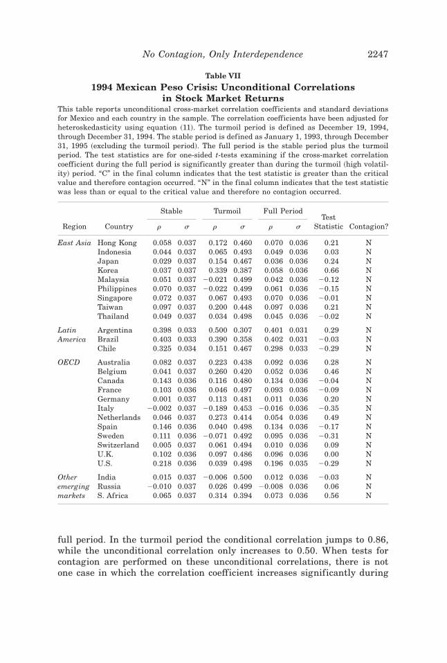
full period. In the turmoil period the conditional correlation jumps to 0.86,while the unconditional correlation only increases to 0.50. When tests forcontagion are performed on these unconditional correlations, there is notone case in which the correlation coefficient increases significantly during

Table VII

1994 Mexican Peso Crisis: Unconditional Correlationsin Stock Market Returns

This table reports unconditional cross-market correlation coefficients and standard deviationsfor Mexico and each country in the sample. The correlation coefficients have been adjusted forheteroskedasticity using equation ~11!. The turmoil period is defined as December 19, 1994,through December 31, 1994. The stable period is defined as January 1, 1993, through December31, 1995 ~excluding the turmoil period!. The full period is the stable period plus the turmoilperiod. The test statistics are for one-sided t-tests examining if the cross-market correlationcoefficient during the full period is significantly greater than during the turmoil ~high volatil-ity! period. “C” in the final column indicates that the test statistic is greater than the criticalvalue and therefore contagion occurred. “N” in the final column indicates that the test statisticwas less than or equal to the critical value and therefore no contagion occurred.




East Asia Hong Kong 0.058 0.037 0.172 0.460 0.070 0.036 0.21 NIndonesia 0.044 0.037 0.065 0.493 0.049 0.036 0.03 NJapan 0.029 0.037 0.154 0.467 0.036 0.036 0.24 NKorea 0.037 0.037 0.339 0.387 0.058 0.036 0.66 NMalaysia 0.051 0.037 20.021 0.499 0.042 0.036 20.12 NPhilippines 0.070 0.037 20.022 0.499 0.061 0.036 20.15 NSingapore 0.072 0.037 0.067 0.493 0.070 0.036 20.01 NTaiwan 0.097 0.037 0.200 0.448 0.097 0.036 0.21 NThailand 0.049 0.037 0.034 0.498 0.045 0.036 20.02 N


Chile 0.325 0.034 0.151 0.467 0.298 0.033 20.29 N

OECD Australia 0.082 0.037 0.223 0.438 0.092 0.036 0.28 NBelgium 0.041 0.037 0.260 0.420 0.052 0.036 0.46 NCanada 0.143 0.036 0.116 0.480 0.134 0.036 20.04 NFrance 0.103 0.036 0.046 0.497 0.093 0.036 20.09 NGermany 0.001 0.037 0.113 0.481 0.011 0.036 0.20 NItaly 20.002 0.037 20.189 0.453 20.016 0.036 20.35 NNetherlands 0.046 0.037 0.273 0.414 0.054 0.036 0.49 NSpain 0.146 0.036 0.040 0.498 0.134 0.036 20.17 NSweden 0.111 0.036 20.071 0.492 0.095 0.036 20.31 NSwitzerland 0.005 0.037 0.061 0.494 0.010 0.036 0.09 NU.K. 0.102 0.036 0.097 0.486 0.096 0.036 0.00 NU.S. 0.218 0.036 0.039 0.498 0.196 0.035 20.29 N

Other India 0.015 0.037 20.006 0.500 0.012 0.036 20.03 Nemerging Russia 20.010 0.037 0.026 0.499 20.008 0.036 0.06 Nmarkets S. Africa 0.065 0.037 0.314 0.394 0.073 0.036 0.56 N


the turmoil period. In other words, according to this testing methodology,there is no longer evidence of a significant change in the magnitude of thepropagation mechanism from Mexico to any other country in the sample.

An extensive set of sensitivity tests supports these results. We modifyperiod definitions, adjust the frequency of returns and lag structure, varythe interest rate controls, and0or estimate local currency returns. In theseries of tests based on the conditional correlation coefficient, there are be-tween zero and seven cases of contagion. Whenever the statistics are ad-justed for heteroskedasticity and tests are based on the unconditionalcorrelation coefficients, however, there is virtually no evidence of conta-gion.22 In other words, there are virtually no cases where the unconditionalcorrelation coefficient between Mexico and any other country in the sampleincreases significantly during the peso crisis.

VI. Contagion during the 1987 U.S. Stock Market Crash

Before the East Asian crisis and Mexican devaluation, another period ofstock market turmoil when investors feared contagion was after the U.S.stock market crash in October 1987. To test for contagion during this period,we repeat the test procedure described above. We define the turmoil periodas October 17, 1987 ~the date the crash began! through December 4, 1987~the nadir of the U.S. market! and define the stable period as January 1,1986, through October 17, 1987. Since many of the smaller stock markets inour sample of 28 countries were not in existence or were highly regulated atthis time, we focus only on the 10 largest stock markets ~including the UnitedStates!. Once again, we focus on two-day, rolling-average, U.S. dollar re-turns and control for five lags of returns and interest rates. Results based onthe conditional and unconditional correlation coefficients are reported inTables VIII and IX. We also perform an extensive set of sensitivity tests inwhich we modify period definitions, adjust the frequency of returns and lagstructure, vary the interest rate controls, and utilize local currency returns.Results are virtually identical to those reported in Tables VIII and IX.

Most patterns are similar to those found after the 1997 East Asian crisisand the 1994 Mexican devaluation. Tests for a significant increase in cross-market correlations based on the conditional correlation coefficients show asubstantial amount of contagion—usually in about one-third to one-half thesample. This agrees with the findings of earlier work testing for contagionafter the 1987 U.S. stock market crash ~and discussed at the start of Sec-tion I!. None of this work using correlation coefficients, however, attemptedto correct for heteroskedasticity and estimate the unconditional correlations

22 In all of these tests based on the unconditional coefficients, there are never more than twocases of contagion. These cases only occur when returns are measured in local currency, andoften occur in countries that are geographically distant from the source of contagion, such asIndia and South Africa.


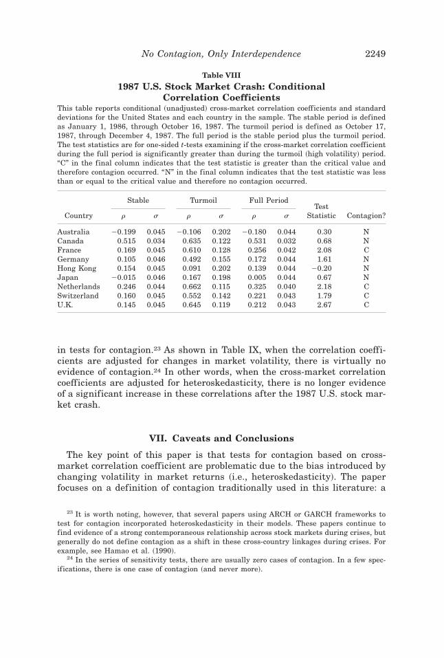
in tests for contagion.23 As shown in Table IX, when the correlation coeffi-cients are adjusted for changes in market volatility, there is virtually noevidence of contagion.24 In other words, when the cross-market correlationcoefficients are adjusted for heteroskedasticity, there is no longer evidenceof a significant increase in these correlations after the 1987 U.S. stock mar-ket crash.

VII. Caveats and Conclusions

The key point of this paper is that tests for contagion based on cross-market correlation coefficient are problematic due to the bias introduced bychanging volatility in market returns ~i.e., heteroskedasticity!. The paperfocuses on a definition of contagion traditionally used in this literature: a

23 It is worth noting, however, that several papers using ARCH or GARCH frameworks totest for contagion incorporated heteroskedasticity in their models. These papers continue tofind evidence of a strong contemporaneous relationship across stock markets during crises, butgenerally do not define contagion as a shift in these cross-country linkages during crises. Forexample, see Hamao et al. ~1990!.

24 In the series of sensitivity tests, there are usually zero cases of contagion. In a few spec-ifications, there is one case of contagion ~and never more!.

Table VIII

1987 U.S. Stock Market Crash: ConditionalCorrelation Coefficients

This table reports conditional ~unadjusted! cross-market correlation coefficients and standarddeviations for the United States and each country in the sample. The stable period is definedas January 1, 1986, through October 16, 1987. The turmoil period is defined as October 17,1987, through December 4, 1987. The full period is the stable period plus the turmoil period.The test statistics are for one-sided t-tests examining if the cross-market correlation coefficientduring the full period is significantly greater than during the turmoil ~high volatility! period.“C” in the final column indicates that the test statistic is greater than the critical value andtherefore contagion occurred. “N” in the final column indicates that the test statistic was lessthan or equal to the critical value and therefore no contagion occurred.


Country r s r s r sTest


Australia 20.199 0.045 20.106 0.202 20.180 0.044 0.30 NCanada 0.515 0.034 0.635 0.122 0.531 0.032 0.68 NFrance 0.169 0.045 0.610 0.128 0.256 0.042 2.08 CGermany 0.105 0.046 0.492 0.155 0.172 0.044 1.61 NHong Kong 0.154 0.045 0.091 0.202 0.139 0.044 20.20 NJapan 20.015 0.046 0.167 0.198 0.005 0.044 0.67 NNetherlands 0.246 0.044 0.662 0.115 0.325 0.040 2.18 CSwitzerland 0.160 0.045 0.552 0.142 0.221 0.043 1.79 CU.K. 0.145 0.045 0.645 0.119 0.212 0.043 2.67 C


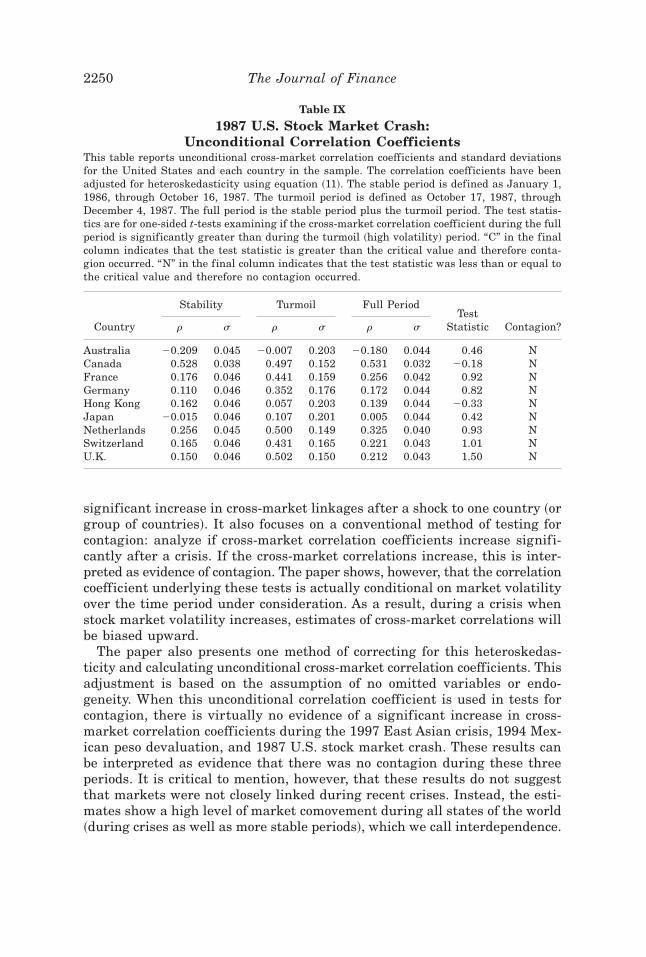
significant increase in cross-market linkages after a shock to one country ~orgroup of countries!. It also focuses on a conventional method of testing forcontagion: analyze if cross-market correlation coefficients increase signifi-cantly after a crisis. If the cross-market correlations increase, this is inter-preted as evidence of contagion. The paper shows, however, that the correlationcoefficient underlying these tests is actually conditional on market volatilityover the time period under consideration. As a result, during a crisis whenstock market volatility increases, estimates of cross-market correlations willbe biased upward.

The paper also presents one method of correcting for this heteroskedas-ticity and calculating unconditional cross-market correlation coefficients. Thisadjustment is based on the assumption of no omitted variables or endo-geneity. When this unconditional correlation coefficient is used in tests forcontagion, there is virtually no evidence of a significant increase in cross-market correlation coefficients during the 1997 East Asian crisis, 1994 Mex-ican peso devaluation, and 1987 U.S. stock market crash. These results canbe interpreted as evidence that there was no contagion during these threeperiods. It is critical to mention, however, that these results do not suggestthat markets were not closely linked during recent crises. Instead, the esti-mates show a high level of market comovement during all states of the world~during crises as well as more stable periods!, which we call interdependence.

Table IX

1987 U.S. Stock Market Crash:Unconditional Correlation Coefficients

This table reports unconditional cross-market correlation coefficients and standard deviationsfor the United States and each country in the sample. The correlation coefficients have beenadjusted for heteroskedasticity using equation ~11!. The stable period is defined as January 1,1986, through October 16, 1987. The turmoil period is defined as October 17, 1987, throughDecember 4, 1987. The full period is the stable period plus the turmoil period. The test statis-tics are for one-sided t-tests examining if the cross-market correlation coefficient during the fullperiod is significantly greater than during the turmoil ~high volatility! period. “C” in the finalcolumn indicates that the test statistic is greater than the critical value and therefore conta-gion occurred. “N” in the final column indicates that the test statistic was less than or equal tothe critical value and therefore no contagion occurred.

Stability Turmoil Full Period

Country r s r s r sTest


Australia 20.209 0.045 20.007 0.203 20.180 0.044 0.46 NCanada 0.528 0.038 0.497 0.152 0.531 0.032 20.18 NFrance 0.176 0.046 0.441 0.159 0.256 0.042 0.92 NGermany 0.110 0.046 0.352 0.176 0.172 0.044 0.82 NHong Kong 0.162 0.046 0.057 0.203 0.139 0.044 20.33 NJapan 20.015 0.046 0.107 0.201 0.005 0.044 0.42 NNetherlands 0.256 0.045 0.500 0.149 0.325 0.040 0.93 NSwitzerland 0.165 0.046 0.431 0.165 0.221 0.043 1.01 NU.K. 0.150 0.046 0.502 0.150 0.212 0.043 1.50 N


This paper only focuses on adjusting for one problem with the cross-market correlation coefficient: heteroskedasticity. While the proposed ad-justment for heteroskedasticity is clearly an improvement over past work, itis only a first step. The adjustment can change in the presence of endo-geneity and0or omitted variables. As shown in Appendix B, it is impossible topredict the extent of this bias in the conditional correlation coefficient whenheteroskedasticity is combined with either of these problems. Future workneeds to examine how endogeneity and omitted variables, especially whencombined with heteroskedasticity, can affect cross-market correlation coef-ficients and tests for contagion.

Finally, the main objective of this paper and its extensive series of tests isto show that inferences based on the conditional correlation coefficient canbe extremely misleading. A simple adjustment for heteroskedasticity can re-verse what appear to be straightforward conclusions about the existence ofcontagion during recent currency crises.

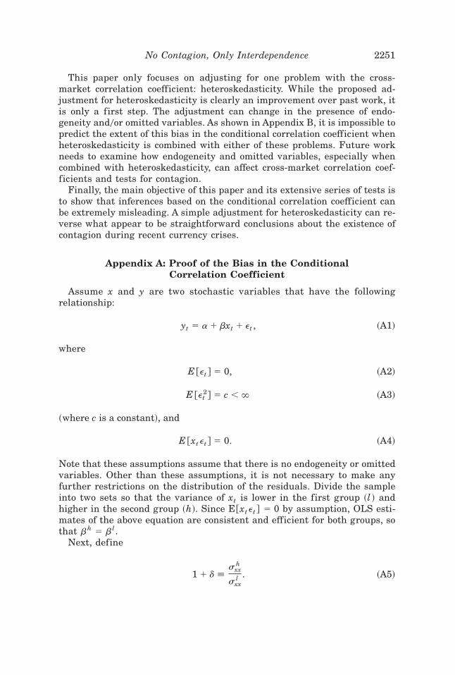
Appendix A: Proof of the Bias in the ConditionalCorrelation Coefficient

Assume x and y are two stochastic variables that have the followingrelationship:

yt 5 a 1 bxt 1 et , ~A1!

where

E @et # 5 0, ~A2!

E @et2# 5 c , ` ~A3!

~where c is a constant!, and

E @xt et # 5 0. ~A4!

Note that these assumptions assume that there is no endogeneity or omittedvariables. Other than these assumptions, it is not necessary to make anyfurther restrictions on the distribution of the residuals. Divide the sampleinto two sets so that the variance of xt is lower in the first group ~l ! andhigher in the second group ~h!. Since E@xt et # 5 0 by assumption, OLS esti-mates of the above equation are consistent and efficient for both groups, sothat bh 5 b l.

Next, define

1 1 d [sxx

h

sxxl . ~A5!


Then

syyh 5 b2sxx

h 1 see

5 b2~1 1 d!sxxl 1 see

5 ~b2sxxl 1 see! 1 db2sxx

l ~A6!

5 syyl 1 db2sxx

l

5 syyl S1 1 db2

sxxl

syyl D,

and when this is combined with

r 5sxy

sx sy5 b

sx

sy~A7!

then

syyh 5 syy

l ~1 1 d@ r l # 2 !. ~A8!

Therefore,

rh 5sxy

h

sxh sy

h

5~1 1 d!sxy

l

~1 1 d!102sxl~1 1 d@ r l # 2 !102sy

l ~A9!

5 r l! 1 1 d

1 1 d@ r l # 2 .

The correlation coefficient is clearly an increasing function of d.

Appendix B: Misspecification Due to Omitted Variablesand Endogeneity

In the main text, we use the simple, stylized model in equations ~1! through~11! to highlight the properties of the conditional correlation coefficient. Weshow that correlation coefficients can be biased in the presence of hetero-skedasticity. The model assumes that there are no omitted variables or endo-geneity. These two assumptions are clearly simplifications, and this appendixexplores their importance.


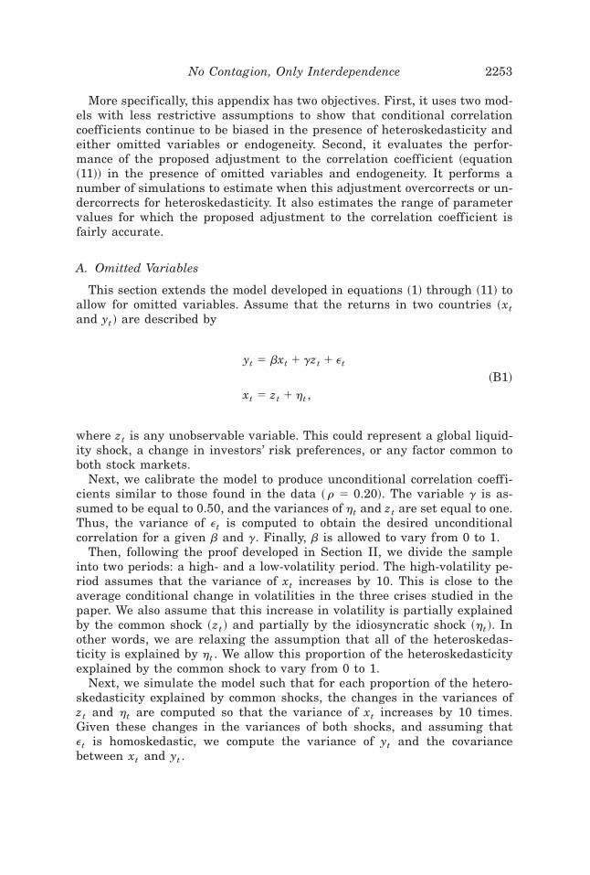
More specifically, this appendix has two objectives. First, it uses two mod-els with less restrictive assumptions to show that conditional correlationcoefficients continue to be biased in the presence of heteroskedasticity andeither omitted variables or endogeneity. Second, it evaluates the perfor-mance of the proposed adjustment to the correlation coefficient ~equation~11!! in the presence of omitted variables and endogeneity. It performs anumber of simulations to estimate when this adjustment overcorrects or un-dercorrects for heteroskedasticity. It also estimates the range of parametervalues for which the proposed adjustment to the correlation coefficient isfairly accurate.

A. Omitted Variables

This section extends the model developed in equations ~1! through ~11! toallow for omitted variables. Assume that the returns in two countries ~xtand yt ! are described by

yt 5 bxt 1 gzt 1 et

xt 5 zt 1 ht ,~B1!

where zt is any unobservable variable. This could represent a global liquid-ity shock, a change in investors’ risk preferences, or any factor common toboth stock markets.

Next, we calibrate the model to produce unconditional correlation coeffi-cients similar to those found in the data ~ r 5 0.20!. The variable g is as-sumed to be equal to 0.50, and the variances of ht and zt are set equal to one.Thus, the variance of et is computed to obtain the desired unconditionalcorrelation for a given b and g. Finally, b is allowed to vary from 0 to 1.

Then, following the proof developed in Section II, we divide the sampleinto two periods: a high- and a low-volatility period. The high-volatility pe-riod assumes that the variance of xt increases by 10. This is close to theaverage conditional change in volatilities in the three crises studied in thepaper. We also assume that this increase in volatility is partially explainedby the common shock ~zt ! and partially by the idiosyncratic shock ~ht !. Inother words, we are relaxing the assumption that all of the heteroskedas-ticity is explained by ht . We allow this proportion of the heteroskedasticityexplained by the common shock to vary from 0 to 1.

Next, we simulate the model such that for each proportion of the hetero-skedasticity explained by common shocks, the changes in the variances ofzt and ht are computed so that the variance of xt increases by 10 times.Given these changes in the variances of both shocks, and assuming thatet is homoskedastic, we compute the variance of yt and the covariancebetween xt and yt .


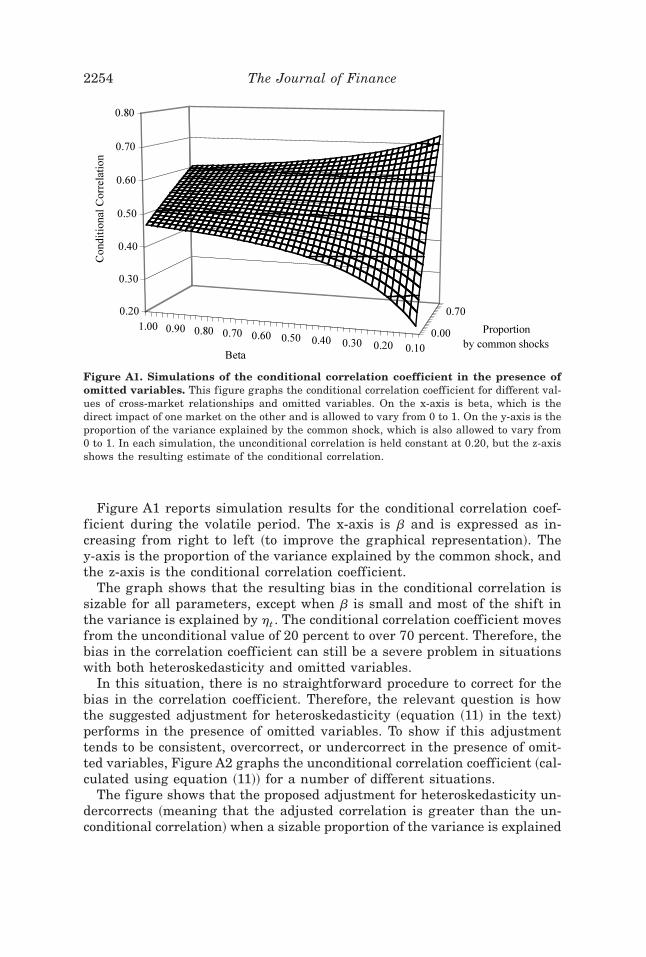
Figure A1 reports simulation results for the conditional correlation coef-ficient during the volatile period. The x-axis is b and is expressed as in-creasing from right to left ~to improve the graphical representation!. They-axis is the proportion of the variance explained by the common shock, andthe z-axis is the conditional correlation coefficient.

The graph shows that the resulting bias in the conditional correlation issizable for all parameters, except when b is small and most of the shift inthe variance is explained by ht . The conditional correlation coefficient movesfrom the unconditional value of 20 percent to over 70 percent. Therefore, thebias in the correlation coefficient can still be a severe problem in situationswith both heteroskedasticity and omitted variables.

In this situation, there is no straightforward procedure to correct for thebias in the correlation coefficient. Therefore, the relevant question is howthe suggested adjustment for heteroskedasticity ~equation ~11! in the text!performs in the presence of omitted variables. To show if this adjustmenttends to be consistent, overcorrect, or undercorrect in the presence of omit-ted variables, Figure A2 graphs the unconditional correlation coefficient ~cal-culated using equation ~11!! for a number of different situations.

The figure shows that the proposed adjustment for heteroskedasticity un-dercorrects ~meaning that the adjusted correlation is greater than the un-conditional correlation! when a sizable proportion of the variance is explained

Figure A1. Simulations of the conditional correlation coefficient in the presence ofomitted variables. This figure graphs the conditional correlation coefficient for different val-ues of cross-market relationships and omitted variables. On the x-axis is beta, which is thedirect impact of one market on the other and is allowed to vary from 0 to 1. On the y-axis is theproportion of the variance explained by the common shock, which is also allowed to vary from0 to 1. In each simulation, the unconditional correlation is held constant at 0.20, but the z-axisshows the resulting estimate of the conditional correlation.


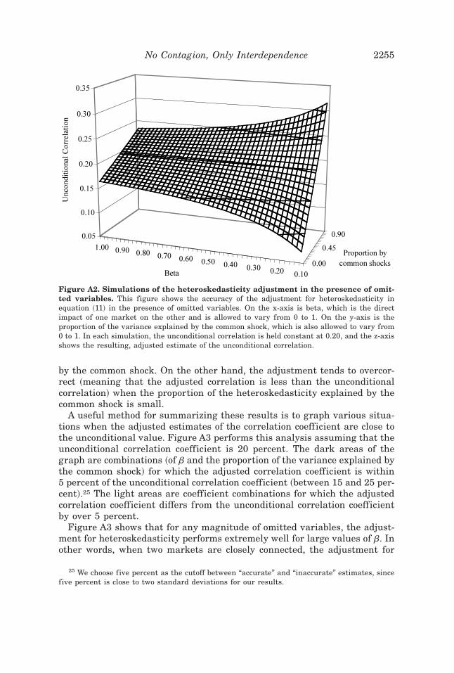
by the common shock. On the other hand, the adjustment tends to overcor-rect ~meaning that the adjusted correlation is less than the unconditionalcorrelation! when the proportion of the heteroskedasticity explained by thecommon shock is small.

A useful method for summarizing these results is to graph various situa-tions when the adjusted estimates of the correlation coefficient are close tothe unconditional value. Figure A3 performs this analysis assuming that theunconditional correlation coefficient is 20 percent. The dark areas of thegraph are combinations ~of b and the proportion of the variance explained bythe common shock! for which the adjusted correlation coefficient is within5 percent of the unconditional correlation coefficient ~between 15 and 25 per-cent!.25 The light areas are coefficient combinations for which the adjustedcorrelation coefficient differs from the unconditional correlation coefficientby over 5 percent.

Figure A3 shows that for any magnitude of omitted variables, the adjust-ment for heteroskedasticity performs extremely well for large values of b. Inother words, when two markets are closely connected, the adjustment for

25 We choose five percent as the cutoff between “accurate” and “inaccurate” estimates, sincefive percent is close to two standard deviations for our results.

Figure A2. Simulations of the heteroskedasticity adjustment in the presence of omit-ted variables. This figure shows the accuracy of the adjustment for heteroskedasticity inequation ~11! in the presence of omitted variables. On the x-axis is beta, which is the directimpact of one market on the other and is allowed to vary from 0 to 1. On the y-axis is theproportion of the variance explained by the common shock, which is also allowed to vary from0 to 1. In each simulation, the unconditional correlation is held constant at 0.20, and the z-axisshows the resulting, adjusted estimate of the unconditional correlation.


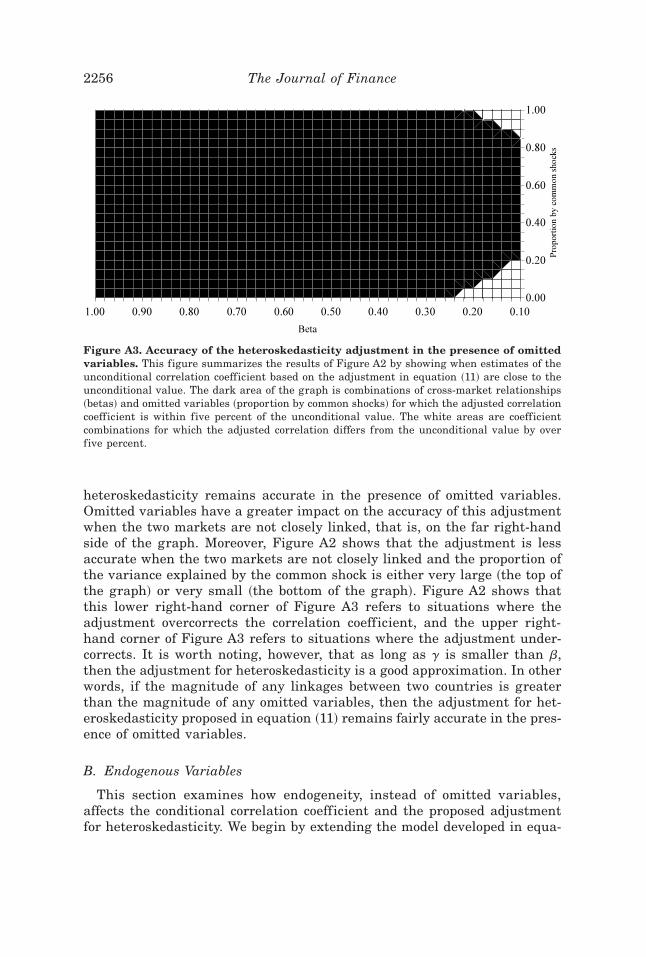
heteroskedasticity remains accurate in the presence of omitted variables.Omitted variables have a greater impact on the accuracy of this adjustmentwhen the two markets are not closely linked, that is, on the far right-handside of the graph. Moreover, Figure A2 shows that the adjustment is lessaccurate when the two markets are not closely linked and the proportion ofthe variance explained by the common shock is either very large ~the top ofthe graph! or very small ~the bottom of the graph!. Figure A2 shows thatthis lower right-hand corner of Figure A3 refers to situations where theadjustment overcorrects the correlation coefficient, and the upper right-hand corner of Figure A3 refers to situations where the adjustment under-corrects. It is worth noting, however, that as long as g is smaller than b,then the adjustment for heteroskedasticity is a good approximation. In otherwords, if the magnitude of any linkages between two countries is greaterthan the magnitude of any omitted variables, then the adjustment for het-eroskedasticity proposed in equation ~11! remains fairly accurate in the pres-ence of omitted variables.

B. Endogenous Variables

This section examines how endogeneity, instead of omitted variables,affects the conditional correlation coefficient and the proposed adjustmentfor heteroskedasticity. We begin by extending the model developed in equa-

Figure A3. Accuracy of the heteroskedasticity adjustment in the presence of omittedvariables. This figure summarizes the results of Figure A2 by showing when estimates of theunconditional correlation coefficient based on the adjustment in equation ~11! are close to theunconditional value. The dark area of the graph is combinations of cross-market relationships~betas! and omitted variables ~proportion by common shocks! for which the adjusted correlationcoefficient is within five percent of the unconditional value. The white areas are coefficientcombinations for which the adjusted correlation differs from the unconditional value by overfive percent.


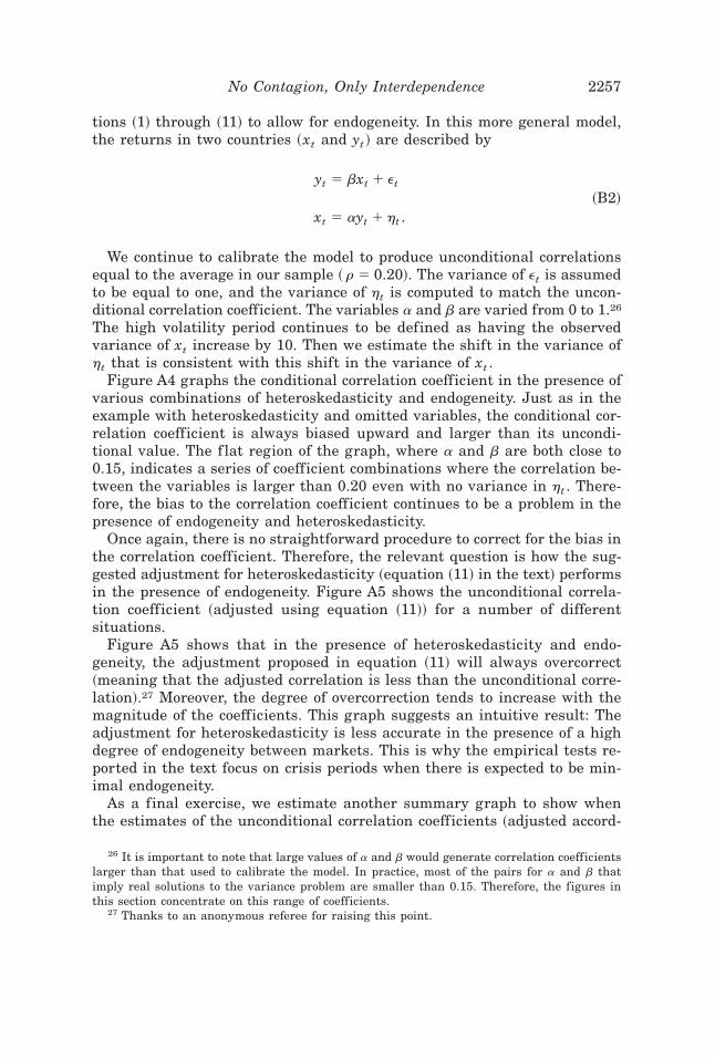
tions ~1! through ~11! to allow for endogeneity. In this more general model,the returns in two countries ~xt and yt ! are described by

yt 5 bxt 1 et

xt 5 ayt 1 ht .~B2!

We continue to calibrate the model to produce unconditional correlationsequal to the average in our sample ~ r 5 0.20!. The variance of et is assumedto be equal to one, and the variance of ht is computed to match the uncon-ditional correlation coefficient. The variables a and b are varied from 0 to 1.26

The high volatility period continues to be defined as having the observedvariance of xt increase by 10. Then we estimate the shift in the variance ofht that is consistent with this shift in the variance of xt .

Figure A4 graphs the conditional correlation coefficient in the presence ofvarious combinations of heteroskedasticity and endogeneity. Just as in theexample with heteroskedasticity and omitted variables, the conditional cor-relation coefficient is always biased upward and larger than its uncondi-tional value. The f lat region of the graph, where a and b are both close to0.15, indicates a series of coefficient combinations where the correlation be-tween the variables is larger than 0.20 even with no variance in ht . There-fore, the bias to the correlation coefficient continues to be a problem in thepresence of endogeneity and heteroskedasticity.

Once again, there is no straightforward procedure to correct for the bias inthe correlation coefficient. Therefore, the relevant question is how the sug-gested adjustment for heteroskedasticity ~equation ~11! in the text! performsin the presence of endogeneity. Figure A5 shows the unconditional correla-tion coefficient ~adjusted using equation ~11!! for a number of differentsituations.

Figure A5 shows that in the presence of heteroskedasticity and endo-geneity, the adjustment proposed in equation ~11! will always overcorrect~meaning that the adjusted correlation is less than the unconditional corre-lation!.27 Moreover, the degree of overcorrection tends to increase with themagnitude of the coefficients. This graph suggests an intuitive result: Theadjustment for heteroskedasticity is less accurate in the presence of a highdegree of endogeneity between markets. This is why the empirical tests re-ported in the text focus on crisis periods when there is expected to be min-imal endogeneity.

As a final exercise, we estimate another summary graph to show whenthe estimates of the unconditional correlation coefficients ~adjusted accord-

26 It is important to note that large values of a and b would generate correlation coefficientslarger than that used to calibrate the model. In practice, most of the pairs for a and b thatimply real solutions to the variance problem are smaller than 0.15. Therefore, the figures inthis section concentrate on this range of coefficients.

27 Thanks to an anonymous referee for raising this point.


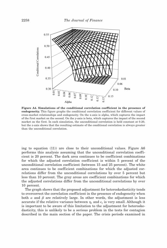
ing to equation ~11!! are close to their unconditional values. Figure A6performs this analysis assuming that the unconditional correlation coeffi-cient is 20 percent. The dark area continues to be coefficient combinationsfor which the adjusted correlation coefficient is within 5 percent of theunconditional correlation coefficient ~between 15 and 25 percent!. The whitearea continues to be coefficient combinations for which the adjusted cor-relations differ from the unconditional correlations by over 5 percent butless than 10 percent. The gray areas are coefficient combinations for whichthe adjusted correlations differ from the unconditional correlations by over10 percent.

The graph shows that the proposed adjustment for heteroskedasticity tendsto overcorrect the correlation coefficient in the presence of endogeneity whenboth a and b are relatively large. In other words, the adjustment is lessaccurate if the relative variance between ht and et is very small. Although itis important to be aware of this limitation to the adjustment for heteroske-dasticity, this is unlikely to be a serious problem in the tests for contagiondescribed in the main section of the paper. The crisis periods examined in

Figure A4. Simulations of the conditional correlation coefficient in the presence ofendogeneity. This figure graphs the conditional correlation coefficient for different values ofcross-market relationships and endogeneity. On the x-axis is alpha, which captures the impactof the first market on the second. On the y-axis is beta, which captures the impact of the secondmarket on the first. In each simulation, the unconditional correlation is held constant at 0.20,but the z-axis shows that the resulting estimate of the conditional correlation is always greaterthan the unconditional correlation.


the paper only include events where the feedback from the second country tothe crisis country is expected to be small.28

C. Conclusion

In conclusion, this appendix has examined the accuracy of the adjustmentfor heteroskedasticity ~proposed in equation ~11!! in the presence of omittedvariables and endogeneity. It shows that under certain circumstances, theadjustment is less accurate and should be used cautiously. For example, insituations with heteroskedasticity, positive linkages between two economies,and a large aggregate shock ~omitted variable!, the proposed adjustmentcould either over- or undercorrect the unconditional correlation coefficient.In situations with heteroskedasticity and a strong feedback effect from thesecond country to the crisis country ~endogeneity!, the proposed adjustmentwill tend to overcorrect the unconditional correlation coefficient. It also shows,

28 In other situations, when the source of the crisis is less well identified and endogeneitymay be more severe, it may be useful to utilize a Granger causality test to determine the extentof any feedback from each country in the sample to the initial crisis country. Granger causalitytests should be used with caution, however, since serial correlation in stock returns could biastest results.

Figure A5. Simulations of the heteroskedasticity adjustment in the presence of endo-geneity. This figure shows the accuracy of the adjustment for heteroskedasticity in equation~11! in the presence of endogeneity. On the x-axis and y-axis are alpha and beta, which capturethe direct impact of each market on the other market. In each simulation, the unconditionalcorrelation is held constant at 0.20, and the z-axis shows the resulting, adjusted estimate of theunconditional correlation.


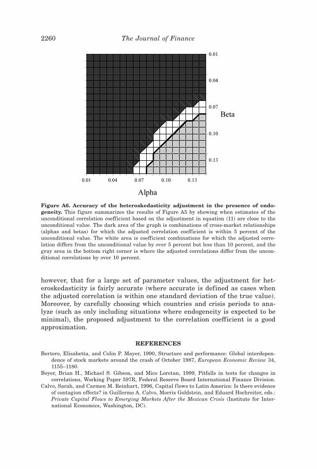
however, that for a large set of parameter values, the adjustment for het-eroskedasticity is fairly accurate ~where accurate is defined as cases whenthe adjusted correlation is within one standard deviation of the true value!.Moreover, by carefully choosing which countries and crisis periods to ana-lyze ~such as only including situations where endogeneity is expected to beminimal!, the proposed adjustment to the correlation coefficient is a goodapproximation.

REFERENCES

Bertero, Elisabetta, and Colin P. Mayer, 1990, Structure and performance: Global interdepen-dence of stock markets around the crash of October 1987, European Economic Review 34,1155–1180.

Boyer, Brian H., Michael S. Gibson, and Mico Loretan, 1999, Pitfalls in tests for changes incorrelations, Working Paper 597R, Federal Reserve Board International Finance Division.

Calvo, Sarah, and Carmen M. Reinhart, 1996, Capital f lows to Latin America: Is there evidenceof contagion effects? in Guillermo A. Calvo, Morris Goldstein, and Eduard Hochreiter, eds.:Private Capital Flows to Emerging Markets After the Mexican Crisis ~Institute for Inter-national Economics, Washington, DC!.

Figure A6. Accuracy of the heteroskedasticity adjustment in the presence of endo-geneity. This figure summarizes the results of Figure A5 by showing when estimates of theunconditional correlation coefficient based on the adjustment in equation ~11! are close to theunconditional value. The dark area of the graph is combinations of cross-market relationships~alphas and betas! for which the adjusted correlation coefficient is within 5 percent of theunconditional value. The white area is coefficient combinations for which the adjusted corre-lation differs from the unconditional value by over 5 percent but less than 10 percent, and thegray area in the bottom right corner is where the adjusted correlations differ from the uncon-ditional correlations by over 10 percent.


Cashin, Paul A., Manmohan Kumar, and C. John McDermott, 1995, International integration ofequity markets and contagion effects, Working Paper 950110, International Monetary Fund.

Chou, Ray Y., Victor K. Ng, and Lynn Pi, 1994, Cointegration of international stock marketindices, Working Paper 94094, International Monetary Fund.

Claessens, Stijn, Rudiger W. Dornbusch, and Yung Chul Park, 2001, Contagion: Why crisesspread and how this can be stopped, in Stijn Claessens, and Kristin J. Forbes, eds.: Inter-national Financial Contagion ~Kluwer Academic Publishers, Norwell, MA!.

Claessens, Stijn, and Kristin J. Forbes, eds., 2001, International Financial Contagion ~KluwerAcademic Publishers, Norwell, MA!.

Edwards, Sebastian, 1998, Interest rate volatility, capital controls, and contagion, WorkingPaper 6756, NBER.

Eichengreen, Barry J., Andrew K. Rose, and Charles A. Wyplosz, 1996, Contagious currencycrises, Scandinavian Journal of Economics 98, 463–484.

Forbes, Kristin J., 2000, The Asian f lu and Russian virus: Firm-level evidence on how crises aretransmitted internationally, Working paper 7807, NBER.

Forbes, Kristin J., and Roberto Rigobon, 2001, Measuring contagion: Conceptual and empiricalissues, in Stijn Claessens, and Kristin J. Forbes, eds.: International Financial Contagion~Kluwer Academic Publishers, Norwell, MA!.

Hamao, Yasushi, Ronald W. Masulis, and Victor K. Ng, 1990, Correlations in price changes andvolatility across international stock markets, The Review of Financial Studies 3, 281–307.

International Finance Corporation, 1997, Emerging Stock Market Factbook ~InternationalFinance Corporation, Washington, DC!.

Karolyi, G. Andrew, and René M. Stulz, 1996, Why do markets move together? An investigationof U.S.-Japan stock return comovements, The Journal of Finance 51, 951–986.

King, Mervyn A., and Sushil Wadhwani, 1990, Transmission of volatility between stock mar-kets, Review of Financial Studies 3, 5–33.

Lee, Sang B., and Kwang Jung Kim, 1993, Does the October 1987 crash strengthen the co-movements among national stock markets? Review of Financial Economics 3, 89–102.

Longin, François M., and Bruno Solnik, 1995, Is the correlation in international equity returnsconstant: 1960–1990? Journal of International Money and Finance 14, 3–26.

Loretan, Mico, and William B. English, 2000, Evaluating “correlation breakdowns” duringperiods of market volatility, in Bank for International Settlements: International FinancialMarkets and the Implications for Monetary and Financial Stability ~Bank for InternationalSettlements, Switzerland!.

Pindyck, Robert S., and Julio J. Rotemberg, 1990, The excess co-movement of commodity prices,The Economic Journal 100, 1173–1189.

Pindyck, Robert S., and Julio J. Rotemberg, 1993, The comovement of stock prices, The Quar-terly Journal of Economics 108, 1073–1104.

Ronn, Ehud I., 1998, The impact of large changes in asset prices on intra-market correlationsin the stock and bond markets, Working paper, University of Texas at Austin.


Documents

No Contagion, Only Interdependence: Measuring Stock Market … · 2015-03-02 · Figure 2. Stock market indices during the 1994 Mexican crisis. This figure graphs stock market indices