No Evidence for Evolution in the Far-Infrared-Radio Correlation

out to z ∼ 2 in the ECDFS

Minnie Y. Mao

Infrared Processing and Analysis Center, California Institute of Technology, Pasadena CA

91125, USA. minnie.mao@csiro.au

School of Mathematics and Physics, University of Tasmania, Private Bag 37, Hobart, 7001,

Australia

CSIRO Astronomy and Space Science, PO Box 76, Epping, NSW, 1710, Australia

Australian Astronomical Observatory, PO Box 296, Epping, NSW, 1710, Australia

Minh T. Huynh

Infrared Processing and Analysis Center, California Institute of Technology, Pasadena CA

91125, USA

International Centre for Radio Astronomy Research, M468, University of Western

Australia, Crawley, WA 6009, Australia

Ray P. Norris

CSIRO Astronomy and Space Science, PO Box 76, Epping, NSW, 1710, Australia

Mark Dickinson

National Optical Astronomy Observatory, 950 North Cherry Avenue, Tucson, AZ 85719,

USA

Dave Frayer

National Radio Astronomy Observatory, PO Box 2, Green Bank, WV 24944, USA

George Helou

Infrared Processing and Analysis Center, California Institute of Technology, Pasadena CA

91125, USA

and

Jacqueline A. Monkiewicz

– 2 –

School of Earth and Space Exploration, Arizona State University, Tempe, AZ 85287, USA

ABSTRACT

We investigate the 70µm Far-Infrared Radio Correlation (FRC) of star-

forming galaxies in the Extended Chandra Deep Field South (ECDFS) out to z

> 2. We use 70µm data from the Far-Infrared Deep Extragalactic Legacy Sur-

vey (FIDEL), which comprises the most sensitive (∼0.8mJy rms) and extensive

far-infrared deep field observations using MIPS on the Spitzer Space Telescope,

and 1.4GHz radio data (∼8µJy beam−1 rms) from the VLA. In order to quantify

the evolution of the FRC we use both survival analysis and stacking techniques

which we find give similar results. We also calculate the FRC using total infrared

luminosity and rest-frame radio luminosity, qTIR, and find that qTIR is constant

(within 0.22) over the redshift range 0 - 2. We see no evidence for evolution in

the FRC at either 70µm or 24µm which is surprising given the many factors

that are expected to change this ratio at high redshifts.

Subject headings: galaxies: evolution, galaxies: formation, infrared radiation,

radio continuum

1. Introduction

The correlation between the far-infrared (FIR) and radio emission for star-forming galax-

ies in the local Universe was first observed by van der Kruit (1971, 1973) and is the tightest

and most universal correlation known among global parameters of galaxies (Helou & Bicay

1993). The correlation is linear, spans five orders of magnitude of bolometric luminosity and

has been shown to hold for a wide range of Hubble types (de Jong et al. 1985; Helou, Soifer

& Rowan-Robinson 1985; Condon 1992; Yun, Reddy & Condon 2001).

The FIR-radio correlation (FRC) has been attributed to the presence of young, high-

mass (M > 8M⊙) stars. The FIR emission arises from the absorption by dust of the UV

emission and subsequent reradiation of the energy at IR wavelengths. The radio emission

is dominated by non-thermal synchrotron emission from cosmic ray electrons which are

accelerated by supernovae shocks. There is also a thermal component which arises from

free-free emission from ionized hydrogen in HII regions, but this contributes only ∼10% of

the radio emission at lower frequencies (<5GHz, Condon 1992), and becomes more significant

at higher frequencies.

– 3 –

The “calorimeter theory” (Voelk 1989) suggests that the FRC holds because galaxies

are both electron calorimeters and UV calorimeters so the total radio and IR outputs remain

proportional independent of variations within the galaxy. This theory however, requires

that galaxies are optically thick to UV light from the young high-mass stars, and thus does

not hold for optically-thin galaxies. Helou & Bicay (1993) proposed the non-calorimetric

“optically thin” scenario involving a correlation between disk scale height and the escape

scale length for cosmic ray electrons, while Bell (2003) concludes that the linearity of the

FRC is a conspiracy as the star-formation rate is underestimated for low-luminosity galaxies

at both radio and infrared frequencies. However, these models typically leave out proton

losses and non-synchrotron cooling (Lacki, Thompson & Quataert 2010). Ultimately, the

physical origin of the FRC is still not clear.

The far-reaching nature of the FRC has made it a valuable diagnostic. Some examples of

its application include: using the FRC to identify radio-loud AGN (Donley et al. 2005; Norris

et al. 2006); using the FRC to define the radio luminosity/SFR relation (Bell 2003); and,

at higher redshifts, using the FRC to estimate distances to submillimeter galaxies without

optical counterparts (e.g., Carilli & Yun 1999). Consequently it is of great importance to

determine whether the FRC holds at high redshifts.

The FRC may fail at high redshifts for a number of reasons. Electrons are expected to

lose energy by inverse Compton interactions with the cosmic microwave background, whose

energy density scales as (1+z)4, implying a lower level of radio emission at higher redshifts.

Moreover, synchrotron emission is proportional to the magnetic field strength squared, so

evolution of magnetic field strength should affect the FRC at higher redshifts (e.g., Murphy

2009). Changes in the spectral energy distributions (SEDs) may also be expected due to

evolution in dust properties and metallicity (e.g., Amblard et al. 2010; Hwang et al. 2010;

Chapman et al. 2010). Nonetheless, current studies show no firm evidence for evolution in

the FRC (e.g., Garrett 2002; Appleton et al. 2004; Seymour et al. 2009; Bourne et al. 2010;

Ivison et al. 2010a,b; Sargent et al. 2010a,b; Huynh et al. 2010).

Herschel was launched in May 2009 and can probe the FIR to submillimeter regime

from 55µm to 671µm, deeper than ever before (Pilbratt et al. 2010). Most recently, Jarvis

et al. (2010) and Ivison et al. (2010b) used data from Herschel and found no evidence for

evolution in the FRC out to z = 0.5 and z = 2 respectively.

This paper studies the dependence of the FRC on redshift using deep 70µm data from

the Spitzer Space Telescope and 1.4GHz data from the Very Large Array (VLA). This work

differs from previous studies as we are using FIDEL (Far-Infrared Deep Extragalactic Legacy

Survey) 70µm data, which is the deepest 70µm data taken to date. FIDEL reaches a point

source rms sensitivity of 0.8mJy at 70µm, making it far more sensitive than previous studies

– 4 –

of the FIR at 70µm such as Sargent et al. (2010b) whose data reached a point source rms

sensitivity of 1.7mJy.

We focus on the 70µm data as this band probes closer to the dust emission peak

(∼100µm) than, for example, 24µm. Furthermore, for z < 3, the 70µm band is not affected

by emission from polycyclic aromatic hydrocarbons (PAHs; 7 - 12 µm). While Bourne et

al. (2010) also study the FRC using FIDEL data, their work was entirely based on stacking

analysis. This work is the first to use such deep 70µm data to study the evolution of the

FRC based on individual sources.

The data are described in Section 2, Section 3 describes the data analysis while Section

4 presents our results and analysis. This paper uses H0 = 71 km s−1 Mpc−1, ΩM = 0.27 and

ΩΛ = 0.73.

2. Data

2.1. FIDEL

FIDEL, the Far-Infrared Deep Extragalactic Legacy Survey, is a legacy science program

(PI: Dickinson) which comprises the most sensitive and extensive FIR deep field observations

using the Multiband Imaging Photometer for SIRTF (MIPS) on the Spitzer Space Telescope.

Characteristics of the FIDEL data are described in detail in Magnelli et al. (2009) and other

papers. FIDEL observed three fields: ECDFS, EGS and GOODS-North. Observations were

taken at 3 bands: 24µm, 70µm and 160µm, focusing specifically on the 70µm data. This

paper concentrates only on the 30′ × 30′ ECDFS field centered on 03 32 00, -27 48 00 (J2000).

The observations were designed to achieve roughly uniform sensitivity at 70µm across most

of the ECDFS, although the FIDEL data include a somewhat deeper central region with

data from a GO program (PI: Frayer). The mean 70µm exposure time over the ECDFS

is approximately 6600s, yielding an RMS point source sensitivity of approximately 0.8mJy.

The 24µm exposure time varies considerably more over the field, from 5000 to 35000 seconds

over most of the ECDFS, with an average exposure time of approximately 16000 seconds.

The RMS point source sensitivity at 24µm thus also varies, but is typically in the range

8 to 14 µJy over most of the field. FIDEL data were processed using the Mosaicking and

Point-source Extraction (MOPEX, Makovoz & Marleau 2005) package to form the mosaicked

images. The final 70µm mosaic has a pixel scale of 4.0 ′′/pixel and a point response function

(PRF) with an 18′′ FWHM. The final 24µm mosaic has a pixel scale of 1.2 ′′/pixel and a

PRF with a 5.9′′ FWHM.

– 5 –

2.2. Ancillary data

2.2.1. Radio data

The ECDFS has been observed at 1.4GHz by both the VLA and the ATCA (Norris et

al. 2006; Kellermann et al. 2008; Miller et al. 2008). Here we use the Miller et al. (2008)

radio data due to its high angular resolution and sensitivity over our field. The radio data

encompass a 34′ × 34′ region, centered on 03 32 28.0, -27 48 30.0 (J2000). The data have

a typical rms sensitivity of 8µJy per 2.8′′ × 1.6′′ beam. The catalog contains 464 sources

above a 7 sigma cutoff.

2.2.2. Redshift data

We obtained both spectroscopic and photometric redshift data from COMBO-17 (Wolf

et al. 2004), MUSYC (Gawiser et al. 2006; Cardamone et al. 2010), GOODS (Balestra et al.

2010) and ATLAS (Mao et al. 2009).

COMBO-17 has photometric data in 17 passbands from 350 nm to 930 nm for 63501

objects in the ECDFS. The photometric redshifts are most reliable for sources with R ≤ 24

(Wolf et al. 2004).

MUSYC (Multiwavelength Survey by Yale-Chile) has photometric data in the ECDFS.

Cardamone et al. (2010) combined photometric data from the literature with new deep 18-

medium-band photometry into a public catalog of ∼80000 galaxies in ECDFS, from which

they computed the photometric redshifts. The photometric redshifts are most reliable for

sources with R ≤ 25.5. Cardamone et al. (2010) also compile a spectroscopic redshift catalog

of 2551 galaxies from the the literature (e.g., Balestra et al. 2010; Vanzella et al. 2008; Le

Fevre et al. 2004).

Balestra et al. (2010) observed the GOODS-South field (within the ECDFS) using VI-

MOS to obtain spectroscopic redshifts. Their campaign used two different grisms to cover

different redshift ranges and used 20 VIMOS masks. They combined their resulting redshifts

with those available in the literature to produce a catalog containing 7332 spectroscopic red-

shifts. Quality flags were provided for all the redshifts and we took only those redshifts that

had quality flags of “secure” and “likely” yielding a catalog of 5528 spectroscopic redshifts.

Although Cardamone et al. (2010) includes Balestra et al. (2010) data in their compilation

of spectroscopic redshifts, they only include a subset of the data.

Mao et al. (2009) are undertaking a program of redshift determination and source classi-

– 6 –

fication of all ATLAS (Australia Telescope Large Area Survey) radio sources with AAOmega

(Sharp et al. 2006) on the Anglo-Australian Telescope (AAT). Using redshifts from both the

literature and their own campaign they have a total of 261 spectroscopic redshifts in ECDFS

and its surrounding region.

2.2.3. X-ray data

We use the 2 Ms Chandra Deep Field South X-ray catalogs from Luo et al. (2008) to

identify AGN in our 70µm catalog (Section 4.1). This is one of the most sensitive X-ray

surveys ever performed and detects 462 sources in 436 arcmin2. While the X-ray data cover

a smaller region than the FIDEL data, we use these data to eliminate some AGN from our

sample (Section 4.1).

3. Data Analysis

3.1. FIDEL

3.1.1. 70µm

The 70µm catalog was produced with the Astronomical Point Source Extraction (APEX)

module within the MOPEX package. APEX subtracts the local background by calculating

the median in a region, which we set to 34 × 34 pixels, surrounding each pixel, and removing

the 100 brightest pixels. Peak values with a S/N greater than three were fitted using the

PRF. The 3-sigma catalog extracted using APEX contained 515 sources.

3.1.2. 24µm

A similar source detection and extraction process to the 70µm data were used for the

24µm data. However a four sigma cutoff was used to reduce the number of spurious sources.

Visual inspection was required to remove spurious sources due to artifacts surrounding bright

objects. The final catalog of 24µm sources in the ∼30′ × 30′ region of interest contained

5319 sources.

– 7 –

3.1.3. Final catalog

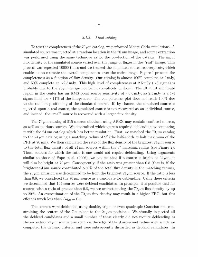
To test the completeness of the 70µm catalog, we performed Monte-Carlo simulations. A

simulated source was injected at a random location in the 70µm image, and source extraction

was performed using the same technique as for the production of the catalog. The input

flux density of the simulated source varied over the range of fluxes in the “real” image. This

process was repeated 10000 times and we tracked the simulated source recovery rate, which

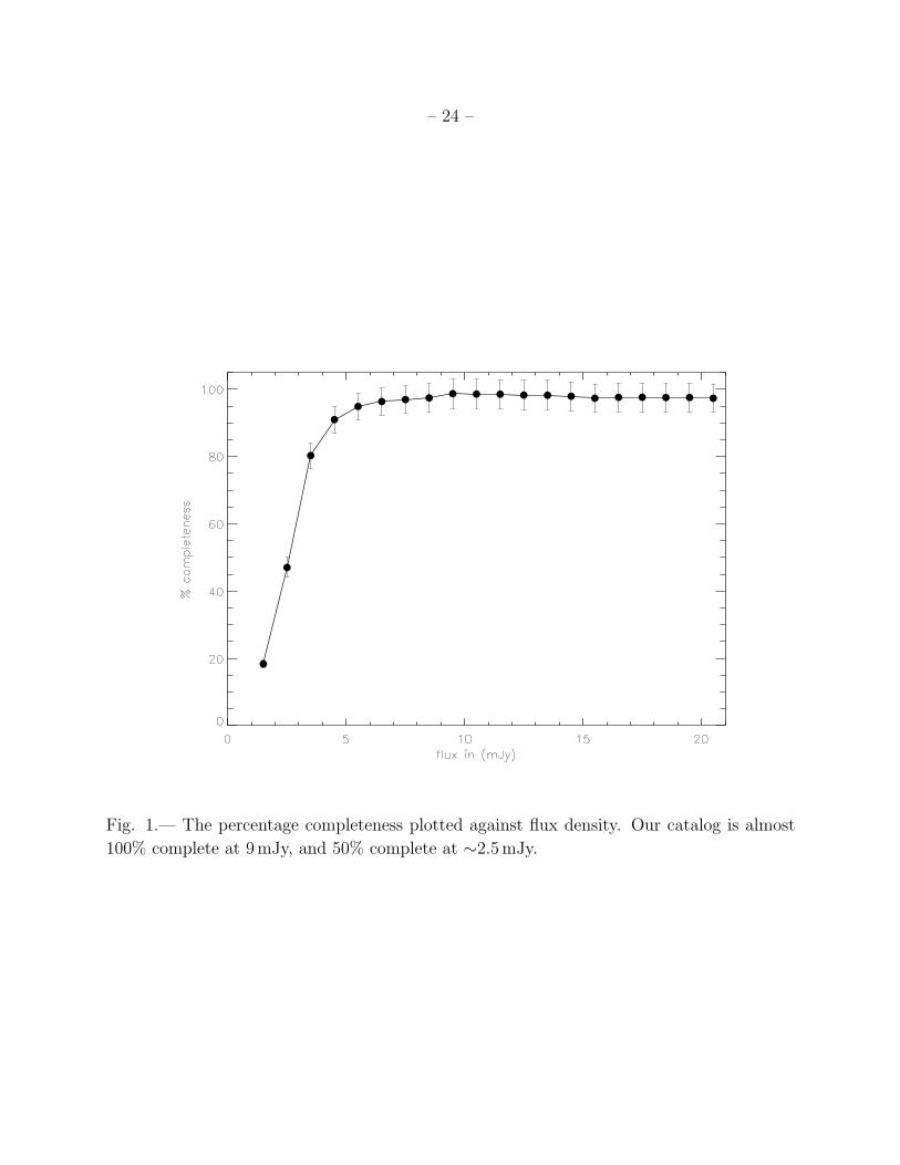
enables us to estimate the overall completeness over the entire image. Figure 1 presents the

completeness as a function of flux density. Our catalog is almost 100% complete at 9mJy,

and 50% complete at ∼2.5mJy. This high level of completeness at 2.5mJy (∼3 sigma) is

probably due to the 70µm image not being completely uniform. The 10 × 10 arcminute

region in the center has an RMS point source sensitivity of ∼0.6mJy, so 2.5mJy is a >4

sigma limit for ∼11% of the image area. The completeness plot does not reach 100% due

to the random positioning of the simulated source. If, by chance, the simulated source is

injected upon a real source, the simulated source is not recovered as an individual source,

and instead, the “real” source is recovered with a larger flux density.

The 70µm catalog of 515 sources obtained using APEX may contain confused sources,

as well as spurious sources. We determined which sources required deblending by comparing

it with the 24µm catalog which has better resolution. First, we matched the 70µm catalog

to the 24µm catalog using a matching radius of 9′′ (the half-width at half maximum of the

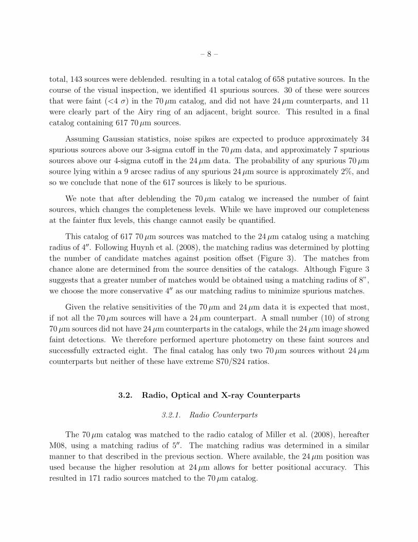
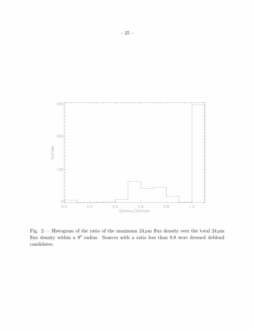
PRF at 70µm). We then calculated the ratio of the flux density of the brightest 24µm source

to the total flux density of all 24µm sources within the 9′′ matching radius (see Figure 2).

Those sources for which the ratio is one would not require deblending. Using arguments

similar to those of Pope et al. (2006), we assume that if a source is bright at 24µm, it

will also be bright at 70µm. Consequently, if the ratio was greater than 0.8 (that is, if the

brightest 24µm source contributed >80% of the total flux density in the matching radius),

the 70µm emission was determined to be from the brightest 24µm source. If the ratio is less

than 0.8, we considered the 70µm source as a candidate for deblending. Using these criteria

we determined that 164 sources were deblend candidates. In principle, it is possible that for

sources with a ratio of greater than 0.8, we are overestimating the 70µm flux density by up

to 20%. An overestimation of the 70µm flux density may result in a higher FRC, but this

effect is much less than ∆q70 = 0.1.

The sources were deblended using double, triple or even quadruple Gaussian fits, con-

straining the centers of the Gaussians to the 24µm positions. We visually inspected all

the deblend candidates and a small number of these clearly did not require deblending as

the secondary 24µm source was right on the edge of the 9 arcsecond radius with which we

computed the deblend criteria, and were subsequently discarded as deblend candidates. In

– 8 –

total, 143 sources were deblended. resulting in a total catalog of 658 putative sources. In the

course of the visual inspection, we identified 41 spurious sources. 30 of these were sources

that were faint (<4 σ) in the 70µm catalog, and did not have 24µm counterparts, and 11

were clearly part of the Airy ring of an adjacent, bright source. This resulted in a final

catalog containing 617 70µm sources.

Assuming Gaussian statistics, noise spikes are expected to produce approximately 34

spurious sources above our 3-sigma cutoff in the 70µm data, and approximately 7 spurious

sources above our 4-sigma cutoff in the 24µm data. The probability of any spurious 70µm

source lying within a 9 arcsec radius of any spurious 24µm source is approximately 2%, and

so we conclude that none of the 617 sources is likely to be spurious.

We note that after deblending the 70µm catalog we increased the number of faint

sources, which changes the completeness levels. While we have improved our completeness

at the fainter flux levels, this change cannot easily be quantified.

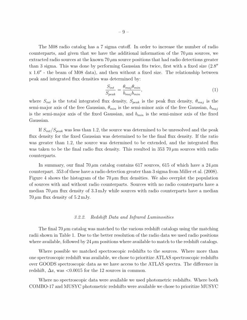
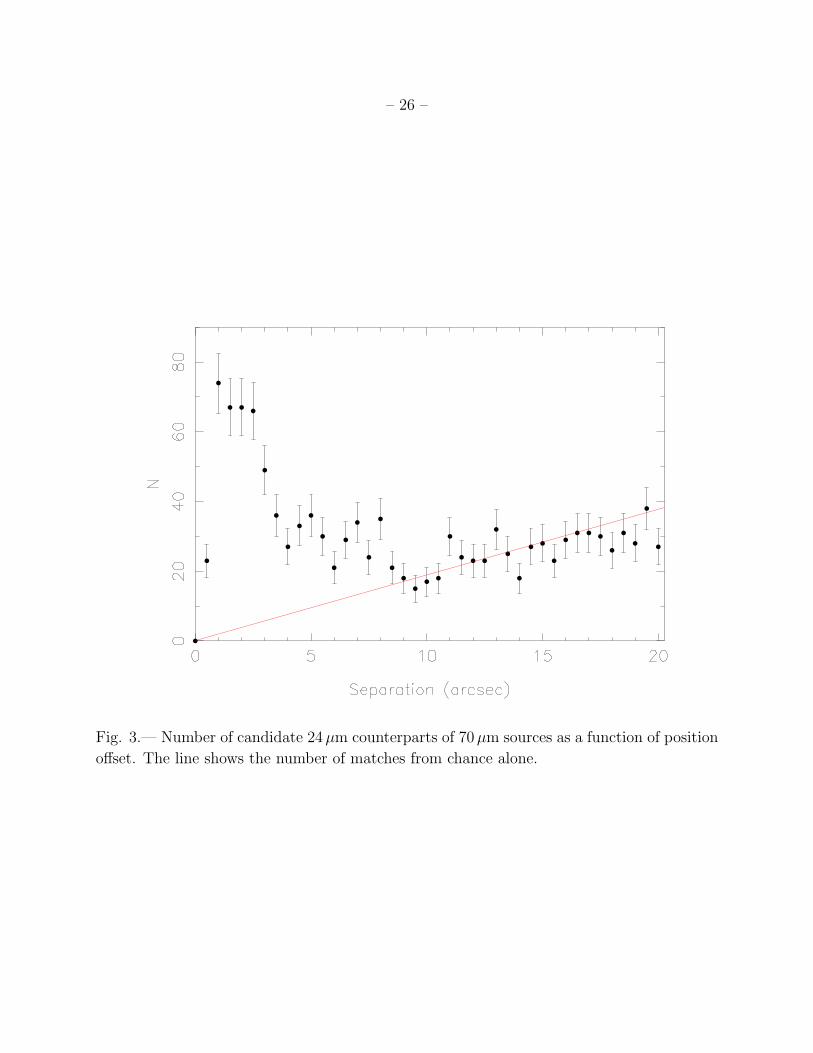
This catalog of 617 70µm sources was matched to the 24µm catalog using a matching

radius of 4′′. Following Huynh et al. (2008), the matching radius was determined by plotting

the number of candidate matches against position offset (Figure 3). The matches from

chance alone are determined from the source densities of the catalogs. Although Figure 3

suggests that a greater number of matches would be obtained using a matching radius of 8”,

we choose the more conservative 4′′ as our matching radius to minimize spurious matches.

Given the relative sensitivities of the 70µm and 24µm data it is expected that most,

if not all the 70µm sources will have a 24µm counterpart. A small number (10) of strong

70µm sources did not have 24µm counterparts in the catalogs, while the 24µm image showed

faint detections. We therefore performed aperture photometry on these faint sources and

successfully extracted eight. The final catalog has only two 70µm sources without 24µm

counterparts but neither of these have extreme S70/S24 ratios.

3.2. Radio, Optical and X-ray Counterparts

3.2.1. Radio Counterparts

The 70µm catalog was matched to the radio catalog of Miller et al. (2008), hereafter

M08, using a matching radius of 5′′. The matching radius was determined in a similar

manner to that described in the previous section. Where available, the 24µm position was

used because the higher resolution at 24µm allows for better positional accuracy. This

resulted in 171 radio sources matched to the 70µm catalog.

– 9 –

The M08 radio catalog has a 7 sigma cutoff. In order to increase the number of radio

counterparts, and given that we have the additional information of the 70µm sources, we

extracted radio sources at the known 70µm source positions that had radio detections greater

than 3 sigma. This was done by performing Gaussian fits twice, first with a fixed size (2.8′′

x 1.6′′ - the beam of M08 data), and then without a fixed size. The relationship between

peak and integrated flux densities was determined by:

Sint

Speak

=θmajθmin

bmajbmin

, (1)

where Sint is the total integrated flux density, Speak is the peak flux density, θmaj is the

semi-major axis of the free Gaussian, θmin is the semi-minor axis of the free Gaussian, bmaj

is the semi-major axis of the fixed Gaussian, and bmin is the semi-minor axis of the fixed

Gaussian.

If Sint/Speak was less than 1.2, the source was determined to be unresolved and the peak

flux density for the fixed Gaussian was determined to be the final flux density. If the ratio

was greater than 1.2, the source was determined to be extended, and the integrated flux

was taken to be the final radio flux density. This resulted in 353 70µm sources with radio

counterparts.

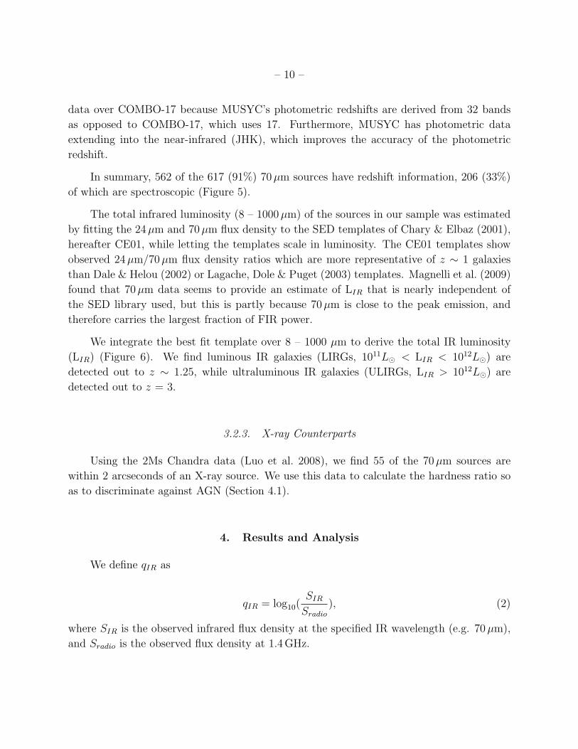
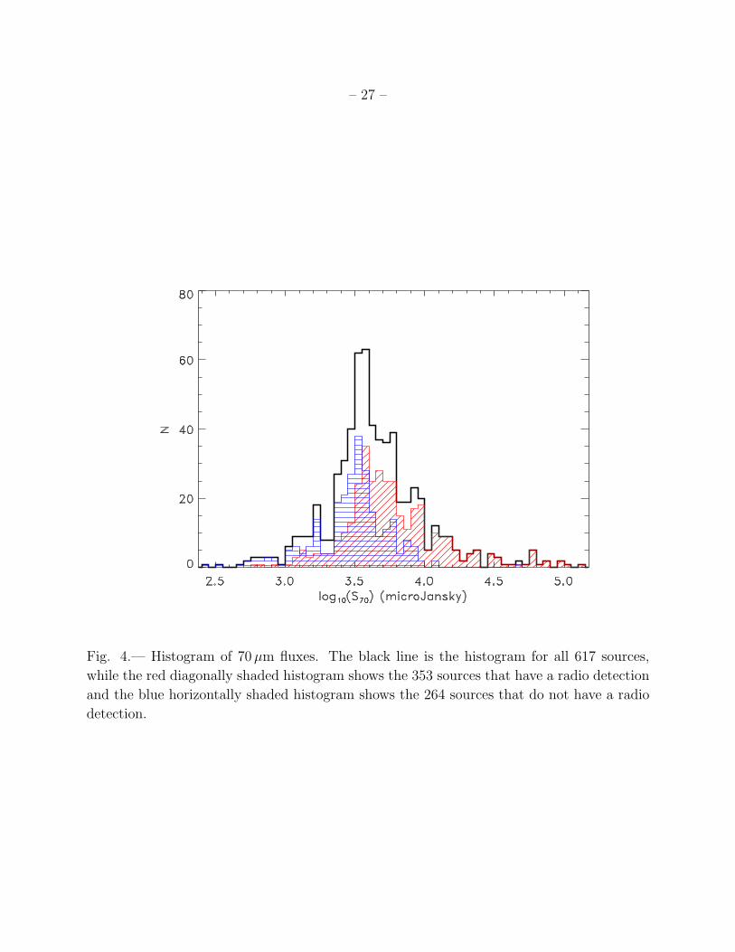
In summary, our final 70µm catalog contains 617 sources, 615 of which have a 24µm

counterpart. 353 of these have a radio detection greater than 3 sigma fromMiller et al. (2008).

Figure 4 shows the histogram of the 70µm flux densities. We also overplot the population

of sources with and without radio counterparts. Sources with no radio counterparts have a

median 70µm flux density of 3.3mJy while sources with radio counterparts have a median

70µm flux density of 5.2mJy.

3.2.2. Redshift Data and Infrared Luminosities

The final 70µm catalog was matched to the various redshift catalogs using the matching

radii shown in Table 1. Due to the better resolution of the radio data we used radio positions

where available, followed by 24µm positions where available to match to the redshift catalogs.

Where possible we matched spectroscopic redshifts to the sources. Where more than

one spectroscopic redshift was available, we chose to prioritize ATLAS spectroscopic redshifts

over GOODS spectroscopic data as we have access to the ATLAS spectra. The difference in

redshift, ∆z, was <0.0015 for the 12 sources in common.

Where no spectroscopic data were available we used photometric redshifts. Where both

COMBO-17 and MUSYC photometric redshifts were available we chose to prioritize MUSYC

– 10 –

data over COMBO-17 because MUSYC’s photometric redshifts are derived from 32 bands

as opposed to COMBO-17, which uses 17. Furthermore, MUSYC has photometric data

extending into the near-infrared (JHK), which improves the accuracy of the photometric

redshift.

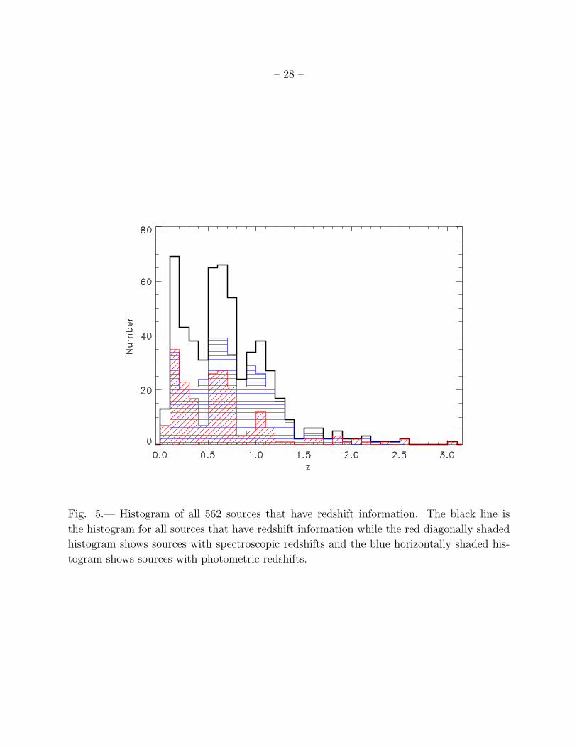
In summary, 562 of the 617 (91%) 70µm sources have redshift information, 206 (33%)

of which are spectroscopic (Figure 5).

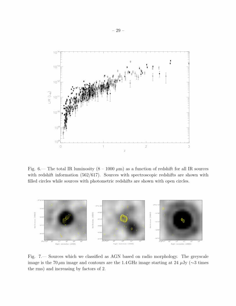
The total infrared luminosity (8 – 1000µm) of the sources in our sample was estimated

by fitting the 24µm and 70µm flux density to the SED templates of Chary & Elbaz (2001),

hereafter CE01, while letting the templates scale in luminosity. The CE01 templates show

observed 24µm/70µm flux density ratios which are more representative of z ∼ 1 galaxies

than Dale & Helou (2002) or Lagache, Dole & Puget (2003) templates. Magnelli et al. (2009)

found that 70µm data seems to provide an estimate of LIR that is nearly independent of

the SED library used, but this is partly because 70µm is close to the peak emission, and

therefore carries the largest fraction of FIR power.

We integrate the best fit template over 8 – 1000 µm to derive the total IR luminosity

(LIR) (Figure 6). We find luminous IR galaxies (LIRGs, 1011L⊙ < LIR < 1012L⊙) are

detected out to z ∼ 1.25, while ultraluminous IR galaxies (ULIRGs, LIR > 1012L⊙) are

detected out to z = 3.

3.2.3. X-ray Counterparts

Using the 2Ms Chandra data (Luo et al. 2008), we find 55 of the 70µm sources are

within 2 arcseconds of an X-ray source. We use this data to calculate the hardness ratio so

as to discriminate against AGN (Section 4.1).

4. Results and Analysis

We define qIR as

qIR = log10(SIR

Sradio

), (2)

where SIR is the observed infrared flux density at the specified IR wavelength (e.g. 70µm),

and Sradio is the observed flux density at 1.4GHz.

– 11 –

4.1. AGN identification

We wish to study the FRC of predominantly star-forming galaxies and so we removed

galaxies from our sample if they satisfied any of the following four criteria which indicate

AGN.

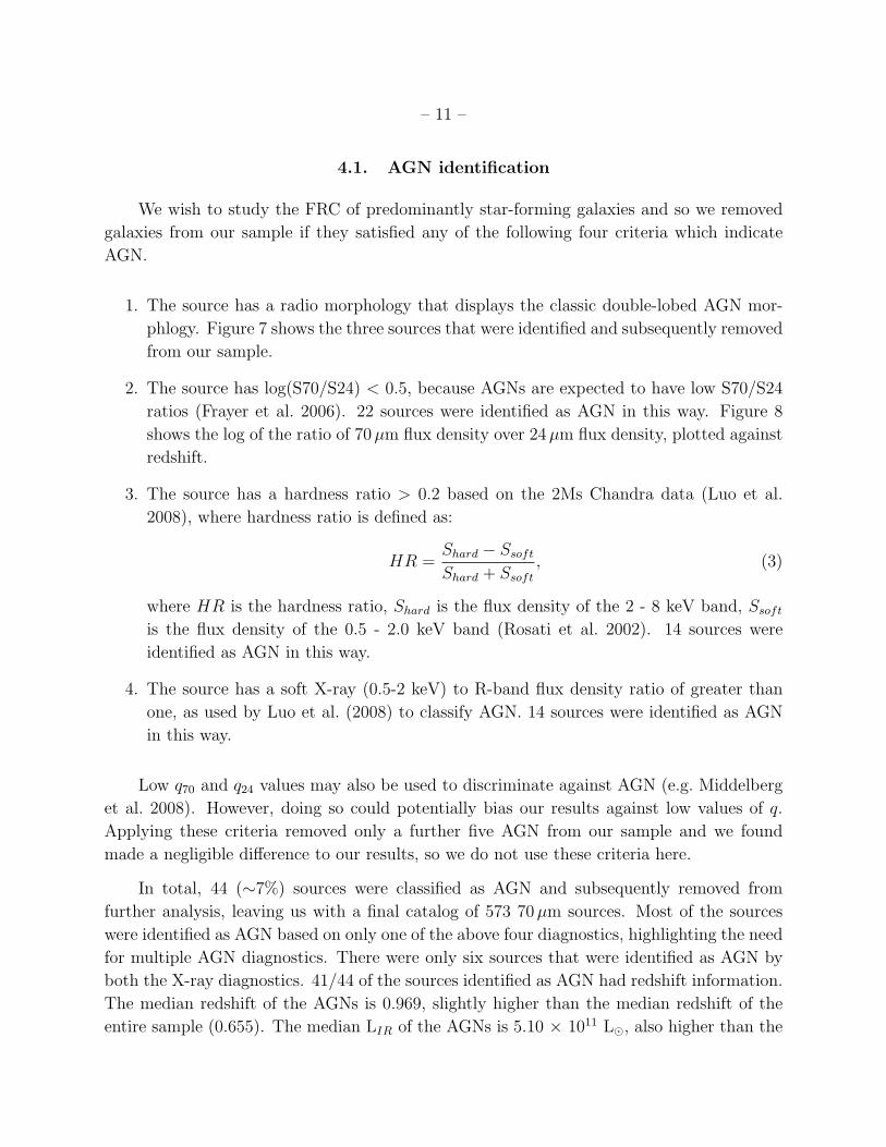
1. The source has a radio morphology that displays the classic double-lobed AGN mor-

phlogy. Figure 7 shows the three sources that were identified and subsequently removed

from our sample.

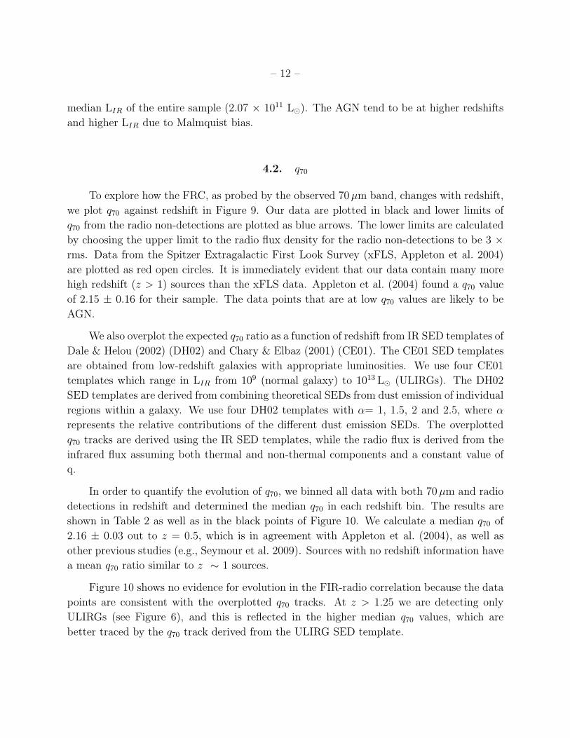
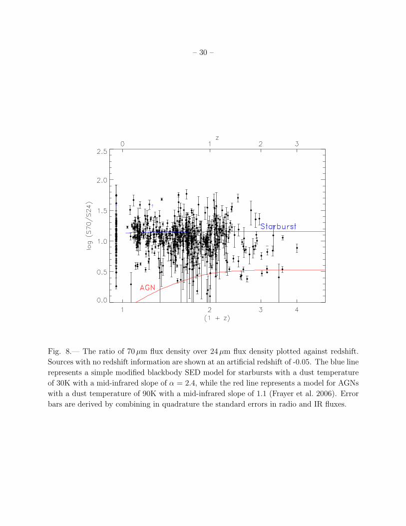
2. The source has log(S70/S24) < 0.5, because AGNs are expected to have low S70/S24

ratios (Frayer et al. 2006). 22 sources were identified as AGN in this way. Figure 8

shows the log of the ratio of 70µm flux density over 24µm flux density, plotted against

redshift.

3. The source has a hardness ratio > 0.2 based on the 2Ms Chandra data (Luo et al.

2008), where hardness ratio is defined as:

HR =Shard − Ssoft

Shard + Ssoft

, (3)

where HR is the hardness ratio, Shard is the flux density of the 2 - 8 keV band, Ssoft

is the flux density of the 0.5 - 2.0 keV band (Rosati et al. 2002). 14 sources were

identified as AGN in this way.

4. The source has a soft X-ray (0.5-2 keV) to R-band flux density ratio of greater than

one, as used by Luo et al. (2008) to classify AGN. 14 sources were identified as AGN

in this way.

Low q70 and q24 values may also be used to discriminate against AGN (e.g. Middelberg

et al. 2008). However, doing so could potentially bias our results against low values of q.

Applying these criteria removed only a further five AGN from our sample and we found

made a negligible difference to our results, so we do not use these criteria here.

In total, 44 (∼7%) sources were classified as AGN and subsequently removed from

further analysis, leaving us with a final catalog of 573 70µm sources. Most of the sources

were identified as AGN based on only one of the above four diagnostics, highlighting the need

for multiple AGN diagnostics. There were only six sources that were identified as AGN by

both the X-ray diagnostics. 41/44 of the sources identified as AGN had redshift information.

The median redshift of the AGNs is 0.969, slightly higher than the median redshift of the

entire sample (0.655). The median LIR of the AGNs is 5.10 × 1011 L⊙, also higher than the

– 12 –

median LIR of the entire sample (2.07 × 1011 L⊙). The AGN tend to be at higher redshifts

and higher LIR due to Malmquist bias.

4.2. q70

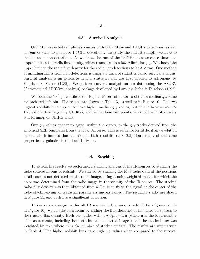
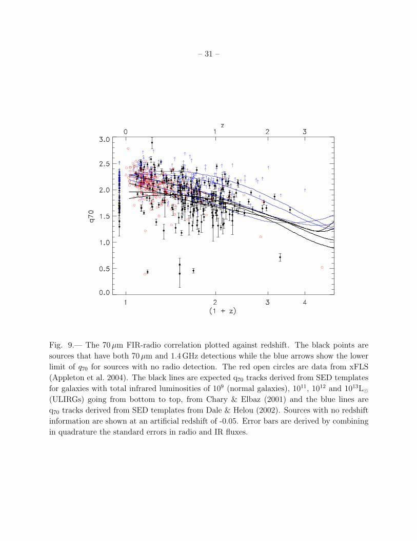
To explore how the FRC, as probed by the observed 70µm band, changes with redshift,

we plot q70 against redshift in Figure 9. Our data are plotted in black and lower limits of

q70 from the radio non-detections are plotted as blue arrows. The lower limits are calculated

by choosing the upper limit to the radio flux density for the radio non-detections to be 3 ×rms. Data from the Spitzer Extragalactic First Look Survey (xFLS, Appleton et al. 2004)

are plotted as red open circles. It is immediately evident that our data contain many more

high redshift (z > 1) sources than the xFLS data. Appleton et al. (2004) found a q70 value

of 2.15 ± 0.16 for their sample. The data points that are at low q70 values are likely to be

AGN.

We also overplot the expected q70 ratio as a function of redshift from IR SED templates of

Dale & Helou (2002) (DH02) and Chary & Elbaz (2001) (CE01). The CE01 SED templates

are obtained from low-redshift galaxies with appropriate luminosities. We use four CE01

templates which range in LIR from 109 (normal galaxy) to 1013 L⊙ (ULIRGs). The DH02

SED templates are derived from combining theoretical SEDs from dust emission of individual

regions within a galaxy. We use four DH02 templates with α= 1, 1.5, 2 and 2.5, where α

represents the relative contributions of the different dust emission SEDs. The overplotted

q70 tracks are derived using the IR SED templates, while the radio flux is derived from the

infrared flux assuming both thermal and non-thermal components and a constant value of

q.

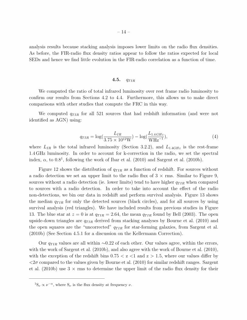
In order to quantify the evolution of q70, we binned all data with both 70µm and radio

detections in redshift and determined the median q70 in each redshift bin. The results are

shown in Table 2 as well as in the black points of Figure 10. We calculate a median q70 of

2.16 ± 0.03 out to z = 0.5, which is in agreement with Appleton et al. (2004), as well as

other previous studies (e.g., Seymour et al. 2009). Sources with no redshift information have

a mean q70 ratio similar to z ∼ 1 sources.

Figure 10 shows no evidence for evolution in the FIR-radio correlation because the data

points are consistent with the overplotted q70 tracks. At z > 1.25 we are detecting only

ULIRGs (see Figure 6), and this is reflected in the higher median q70 values, which are

better traced by the q70 track derived from the ULIRG SED template.

– 13 –

4.3. Survival Analysis

Our 70µm selected sample has sources with both 70µm and 1.4GHz detections, as well

as sources that do not have 1.4GHz detections. To study the full IR sample, we have to

include radio non-detections. As we know the rms of the 1.4GHz data we can estimate an

upper limit to the radio flux density, which translates to a lower limit for q70. We choose the

upper limit to the radio flux density for the radio non-detections to be 3 × rms. One method

of including limits from non-detections is using a branch of statistics called survival analysis.

Survival analysis is an extensive field of statistics and was first applied to astronomy by

Feigelson & Nelson (1985). We perform survival analysis on our data using the ASURV

(Astronomical SURVival analysis) package developed by Lavalley, Isobe & Feigelson (1992).

We took the 50th percentile of the Kaplan-Meier estimator to obtain a median q70 value

for each redshift bin. The results are shown in Table 3, as well as in Figure 10. The two

highest redshift bins appear to have higher median q70 values, but this is because at z >

1.25 we are detecting only ULIRGs, and hence these two points lie along the most actively

star-forming, or ULIRG track.

Our q70 values appear to agree, within the errors, to the q70 tracks derived from the

empirical SED templates from the local Universe. This is evidence for little, if any evolution

in q70, which implies that galaxies at high redshifts (z ∼ 2.5) share many of the same

properties as galaxies in the local Universe.

4.4. Stacking

To extend the results we performed a stacking analysis of the IR sources by stacking the

radio sources in bins of redshift. We started by stacking the M08 radio data at the positions

of all sources not detected in the radio image, using a noise-weighted mean, for which the

noise was determined from the radio image in the vicinity of the IR source. The stacked

radio flux density was then obtained from a Gaussian fit to the signal at the center of the

radio stack, leaving all Gaussian parameters unconstrained. The resulting stacks are shown

in Figure 11, and each has a significant detection.

To derive an average q70 for all IR sources in the various redshift bins (green points

in Figure 10), we calculated a mean by adding the flux densities of the detected sources to

the stacked flux density. Each was added with a weight =1/n (where n is the total number

of measurements, including both stacked and detected images) and the stacked flux was

weighted by m/n where m is the number of stacked images. The results are summarized

in Table 4. The higher redshift bins have higher q values when compared to the survival

– 14 –

analysis results because stacking analysis imposes lower limits on the radio flux densities.

As before, the FIR-radio flux density ratios appear to follow the ratios expected for local

SEDs and hence we find little evolution in the FIR-radio correlation as a function of time.

4.5. qTIR

We computed the ratio of total infrared luminosity over rest frame radio luminosity to

confirm our results from Sections 4.2 to 4.4. Furthermore, this allows us to make direct

comparisons with other studies that compute the FRC in this way.

We computed qTIR for all 521 sources that had redshift information (and were not

identified as AGN) using:

qTIR = log(LIR

3.75× 1012W)− log(

L1.4GHz

WHz−1 ), (4)

where LIR is the total infrared luminosity (Section 3.2.2), and L1.4GHz is the rest-frame

1.4GHz luminosity. In order to account for k-correction in the radio, we set the spectral

index, α, to 0.81, following the work of Ibar et al. (2010) and Sargent et al. (2010b).

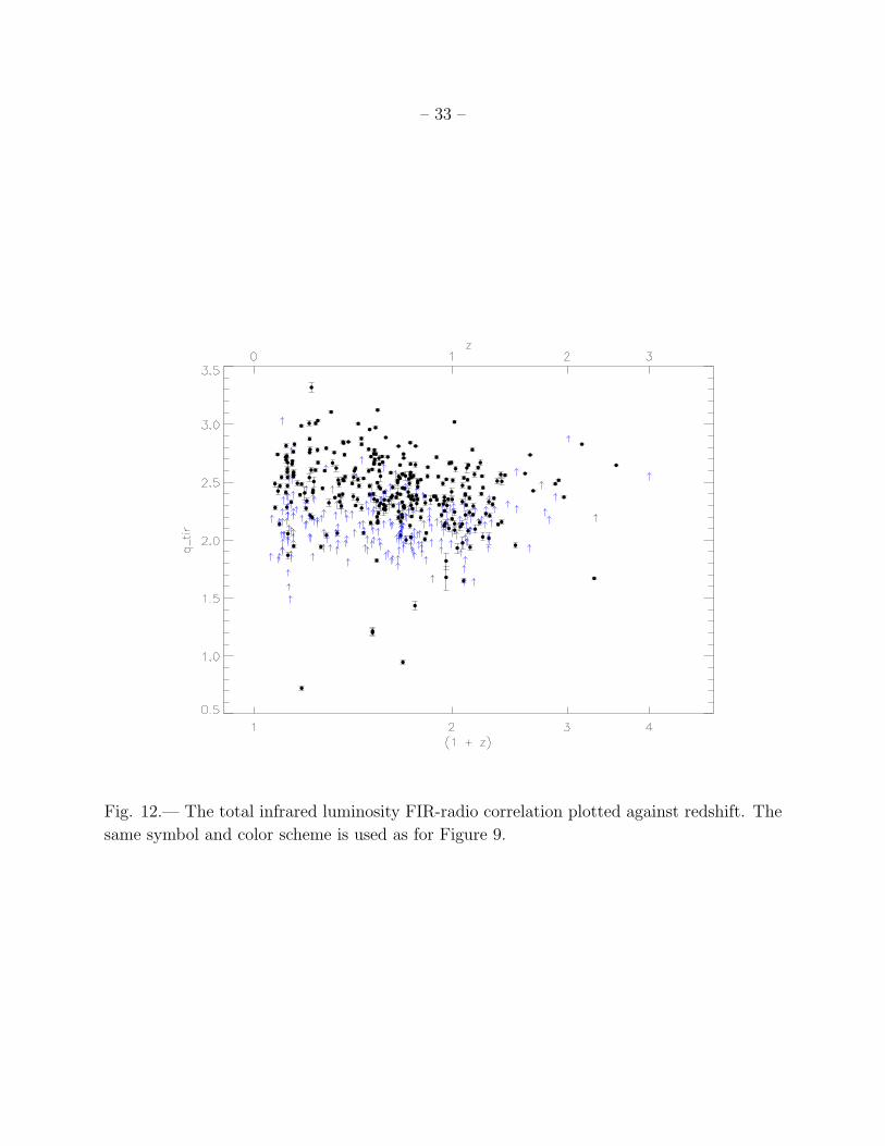
Figure 12 shows the distribution of qTIR as a function of redshift. For sources without

a radio detection we set an upper limit to the radio flux of 3 × rms. Similar to Figure 9,

sources without a radio detection (ie. lower limits) tend to have higher qTIR when compared

to sources with a radio detection. In order to take into account the effect of the radio

non-detections, we bin our data in redshift and perform survival analysis. Figure 13 shows

the median qTIR for only the detected sources (black circles), and for all sources by using

survival analysis (red triangles). We have included results from previous studies in Figure

13. The blue star at z = 0 is at qTIR = 2.64, the mean qTIR found by Bell (2003). The open

upside-down triangles are qTIR derived from stacking analyses by Bourne et al. (2010) and

the open squares are the “uncorrected” qTIR for star-forming galaxies, from Sargent et al.

(2010b) (See Section 4.5.1 for a discussion on the Kellermann Correction).

Our qTIR values are all within ∼0.22 of each other. Our values agree, within the errors,

with the work of Sargent et al. (2010b), and also agree with the work of Bourne et al. (2010),

with the exception of the redshift bins 0.75 < z <1 and z > 1.5, where our values differ by

<2σ compared to the values given by Bourne et al. (2010) for similar redshift ranges. Sargent

et al. (2010b) use 3 × rms to determine the upper limit of the radio flux density for their

1Sν ∝ ν−α, where Sν is the flux density at frequency ν.

– 15 –

dataset. Unlike the work by Bourne et al. (2010) and Sargent et al. (2010b), our qTIR values

do not consistently increase or decrease over the redshift range studied, although we do see

marginally significant evidence for a decreasing qTIR over the redshift range 0 to 1.5, followed

by an increase from 1.5 to 3. However, Fig 14 shows that the data points that use survival

analysis (which are more reliable than those that do not) are statistically consistent with a

horizontal line at about qTIR = 2.62, and so we conclude that these apparent variations of

qTIR with redshift may not be statistically significant.

Bourne et al. (2010) find their qTIR values are systematically higher than the median

qTIR found by Bell (2003) of 2.64 ± 0.02, except at z > 1 where it appears to decline. They

suggest the apparent decline may be attributed to the assumptions they make about spectral

indices. Sargent et al. (2010b) find that their qTIR values are constant with redshift when

they apply a correction (see Section 4.5.1), otherwise ∼0.3 dex of evolution is found. While

Bourne et al. (2010) also uses FIDEL data in the ECDFS, their sample is IRAC selected

whereas our sample is 70µm selected. Sargent et al. (2010b) use a 24µm selected sample to

study the qTIR in the COSMOS field.

There are a number of factors that may contribute to uncertainties in qTIR. The pre-

dominant source of uncertainty is in the estimation of LIR as we are fitting the 24µm and

70µm fluxes to SED templates. The uncertainty from the choice of model SEDs can add

0.2 to 0.3 dex (Magnelli et al. 2009; Le Floc’h et al. 2005). Uncertainties also arise from the

rest-frame radio luminosity where we are assuming α = 0.8.

Jarvis et al. (2010) suggest that the slight upturn in qIR seen at low redshifts (z <

0.5) in high redshift studies of the FRC (e.g. Bourne et al. 2010) may be attributed to the

resolving of extended structure, which means radio flux would be missed and hence increase

the FRC. Our radio data has a 2.8′′ × 1.6′′ beam, so if the Jarvis hypothesis is correct, we

would expect to see this effect at low redshifts.

Although we see a slight upturn in qTIR from z = 1 to z = 0, this increase has a roughly

constant gradient, implying that resolution effects are important as high as z = 1. However,

at z = 1 a typical star-forming galaxy of diameter 10 kpc is unresolved by our beam. Thus,

the increasing qTIR towards low redshifts is probably not due to this effect.

4.5.1. The Kellermann Correction

Kellermann (1964) showed that flux ratios (such as q) or spectral indices of a flux-

limited sample are biased by a factor which depends sensitively on the scatter in the flux

ratio and on the source intensity distribution, and in particular on the power law index β

– 16 –

of the differential source counts (i.e., dN/dS ∝ S−β ). Other formulations of the same effect

are given by Condon (1984), Francis (1993) and Lauer et al. (2007), and were first noted as

being relevant to the evolution of q by Sargent et al. (2010a).

Sargent et al. (2010b) assume a Euclidean (β=2.5) source intensity distribution at z <

1.4 and a sub-Euclidean (β ∼1.5) at 1.4 < z < 2 to derive a correction of 0.22 in their value

of q at z > 1.4. However we note that (a) the expression assumes a common value of β for

both the radio and infrared source counts, and (b) the value of β is very uncertain at low

flux densities. For example, the median radio flux density for our detected sources at z <

1.4 is ∼ 72 µJy, at which the radio source count power law index lies in the range ∼ 1.5 -

2.5 (e.g., Huynh et al. 2005), leading to a correction factor between 0.22 (the adopted value

of Sargent, which gives no evolution of q with z) and 0.51 (which implies that q decreases

with z with marginal significance).

Because of this uncertainty in the value of the Kellermann correction for faint sources

such as those studied here and for consistency with other authors (e.g., Appleton et al. 2004;

Seymour et al. 2009; Bourne et al. 2010), we do not apply it to our data but note that it is

responsible for a further uncertainty in the slope of q as a function of redshift. The range

of possible Kellermann corrections (which depend strongly on the assumed value of β) to

the variation of q over our redshift range is roughly centered on zero, with a total spread of

about ± 0.3.

5. Summary and Conclusions

We have studied the FRC out to z > 2 of ULIRGs in ECDFS. Our results for q70 showed

that they could be broadly described by q70 tracks derived from the SED templates of Chary

& Elbaz (2001) and Dale & Helou (2002). To quantify the evolution of q70 we binned our

data in redshift and determined the median q70 using both survival analysis and a stacking

analysis. Both survival analysis and the stacking analysis gave similar results. We see no

clear evidence for evolution in the FRC at 70µm.

We also calculate the FRC using LIR and L1.4GHz and find that evolution in qTIR is

constrained within 0.22. Our calculated qTIR appears slightly lower than previous studies but

this may merely be due to uncertainties involved in calculating qTIR. We also acknowledge

the importance of the Kellermann correction but due to uncertainties in the value we do not

apply it to our data.

A lack of evolution in the FRC is surprising because it implies that the myriad of effects

on which the FRC rely must either also not evolve, or must evolve in such a way so as

– 17 –

to preserve the FRC. Effects such as inverse Compton cooling of the electrons (Murphy

2009), evolution of the magnetic field strength, and evolution in the SEDs due to dust and

metallicity changes should all affect the FRC.

We therefore conclude that either all these factors are insignificant at z ∼ 2 or there is

a complex interplay between these factors conspiring in the preservation of the FRC at high

redshifts.

Early science results from Herschel have already hinted that the FRC shows no evidence

for evolution to z = 2 (Jarvis et al. 2010; Ivison et al. 2010b). More results on the FRC

from Herschel are expected over the next few years as observations are completed and the

data analyzed. Herschel will measure the far-infrared properties of normal galaxies to z ∼1 and ULIRGs out to z ∼ 4. Consequently, we will be able to study the FRC out to higher

redshifts and hence gain a better understanding of the evolution of star-forming galaxies,

especially in the high redshift Universe.

We wish to thank our anonymous referee whose insightful comments helped improve

this paper. We wish to thank Neal Miller for providing the radio data. MYM was supported

by the IPAC Visiting Graduate Research Fellowship Program for this work.

REFERENCES

Amblard A., et al., 2010, A&A, 518, L9

Appleton P. N., et al., 2004, ApJS, 154, 147

Balestra I., et al., 2010, A&A, 512, A12

Bell E. F., 2003, ApJ, 586, 794

Bourne N., Dunne L., Ivison R. J., Maddox S. J., Dickinson M., Frayer D. T., 2010, MNRAS,

1524

Cardamone C. N., et al., 2010, ApJS, 189, 270

Carilli C. L., Yun M. S., 1999, ApJ, 513, L13

Chapman S. C., et al., 2010, MNRAS, 409, L13

Chary R., Elbaz D., 2001, ApJ, 556, 562

– 18 –

Condon J. J., 1984, ApJ, 287, 461

Condon J. J., 1992, ARA&A, 30, 575

Dale D. A., Helou G., 2002, ApJ, 576, 159

de Jong T., Klein U., Wielebinski R., Wunderlich E., 1985, A&A, 147, L6

Donley J. L., Rieke G. H., Rigby J. R., Perez-Gonzalez P. G., 2005, ApJ, 634, 169

Francis P. J., 1993, ApJ, 407, 519

Garrett M. A., 2002, A&A, 384, L19

Gawiser E., et al., 2006, ApJS, 162, 1

Huynh M. T., Pope A., Frayer D. T., Scott D., 2007, ApJ, 659, 305

Feigelson E. D., Nelson P. I., 1985, ApJ, 293, 192

Frayer D. T., et al., 2006, AJ, 131, 250

Helou G., Soifer B. T., Rowan-Robinson M., 1985, ApJ, 298, L7

Helou G., Bicay M. D., 1993, ApJ, 415, 93

Huynh M. T., Jackson C. A., Norris R. P., Prandoni I., 2005, AJ, 130, 1373

Huynh M. T., Jackson C. A., Norris R. P., Fernandez-Soto A., 2008, AJ, 135, 2470

Huynh M. T., Gawiser E., Marchesini D., Brammer G., Guaita L., 2010, ApJ, 723, 1110

Hwang H. S., et al., 2010, MNRAS, 409, 75

Ibar E., Ivison R. J., Best P. N., Coppin K., Pope A., Smail I., Dunlop J. S., 2010, MNRAS,

401, L53

Ivison R. J., et al., 2010, MNRAS, 402, 245

Ivison R. J., et al., 2010, A&A, 518, L31

Jarvis M. J., et al., 2010, MNRAS, 409, 92

Kellermann K. I., 1964, ApJ, 140, 969

Kellermann K. I., Fomalont E. B., Mainieri V., Padovani P., Rosati P., Shaver P., Tozzi P.,

Miller N., 2008, ApJS, 179, 71

– 19 –

Lacki B. C., Thompson T. A., Quataert E., 2010, ApJ, 717, 1

Lagache G., Dole H., Puget J.-L., 2003, MNRAS, 338, 555

Lauer T. R., Tremaine S., Richstone D., Faber S. M., 2007, ApJ, 670, 249

Lavalley M., Isobe T., Feigelson E., 1992, ASPC, 25, 245

Le Fevre O., et al., 2004, A&A, 428, 1043

Le Floc’h E., et al., 2005, ApJ, 632, 169

Luo B., et al., 2008, ApJS, 179, 19

Magnelli B., Elbaz D., Chary R. R., Dickinson M., Le Borgne D., Frayer D. T., Willmer

C. N. A., 2009, A&A, 496, 57

Makovoz D., Marleau F. R., 2005, PASP, 117, 1113

Mao M. Y., Norris R. P., Sharp R., Lovell J. E. J., 2009, ASPC, 408, 380

Middelberg E., et al., 2008, AJ, 135, 1276

Miller N. A., Fomalont E. B., Kellermann K. I., Mainieri V., Norman C., Padovani P., Rosati

P., Tozzi P., 2008, ApJS, 179, 114

Murphy E. J., 2009, ApJ, 706, 482

Norris R. P., et al., 2006, AJ, 132, 2409

Pilbratt G. L., et al., 2010, A&A, 518, L1

Pope A., et al., 2006, MNRAS, 370, 1185

Rosati P., et al., 2002, ApJ, 566, 667

Sargent M. T., et al., 2010, ApJS, 186, 341

Sargent M. T., et al., 2010, ApJ, 714, L190

Seymour N., Huynh M., Dwelly T., Symeonidis M., Hopkins A., McHardy I. M., Page M. J.,

Rieke G., 2009, MNRAS, 398, 1573

Sharp R., et al., 2006, SPIE, 6269, 14

van der Kruit P. C., 1971, A&A, 15, 110

– 20 –

van der Kruit P. C., 1973, A&A, 29, 263

Vanzella E., et al., 2008, A&A, 478, 83

Voelk H. J., 1989, A&A, 218, 67

Wolf C., et al., 2004, A&A, 421, 913

Yun M. S., Reddy N. A., Condon J. J., 2001, ApJ, 554, 803

This preprint was prepared with the AAS LATEX macros v5.2.

– 21 –

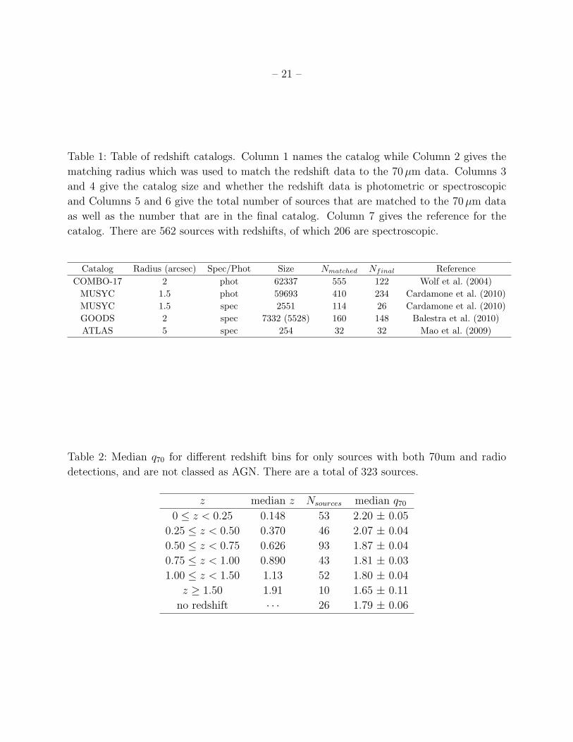
Table 1: Table of redshift catalogs. Column 1 names the catalog while Column 2 gives the

matching radius which was used to match the redshift data to the 70µm data. Columns 3

and 4 give the catalog size and whether the redshift data is photometric or spectroscopic

and Columns 5 and 6 give the total number of sources that are matched to the 70µm data

as well as the number that are in the final catalog. Column 7 gives the reference for the

catalog. There are 562 sources with redshifts, of which 206 are spectroscopic.

Catalog Radius (arcsec) Spec/Phot Size Nmatched Nfinal Reference

COMBO-17 2 phot 62337 555 122 Wolf et al. (2004)

MUSYC 1.5 phot 59693 410 234 Cardamone et al. (2010)

MUSYC 1.5 spec 2551 114 26 Cardamone et al. (2010)

GOODS 2 spec 7332 (5528) 160 148 Balestra et al. (2010)

ATLAS 5 spec 254 32 32 Mao et al. (2009)

Table 2: Median q70 for different redshift bins for only sources with both 70um and radio

detections, and are not classed as AGN. There are a total of 323 sources.

z median z Nsources median q700 ≤ z < 0.25 0.148 53 2.20 ± 0.05

0.25 ≤ z < 0.50 0.370 46 2.07 ± 0.04

0.50 ≤ z < 0.75 0.626 93 1.87 ± 0.04

0.75 ≤ z < 1.00 0.890 43 1.81 ± 0.03

1.00 ≤ z < 1.50 1.13 52 1.80 ± 0.04

z ≥ 1.50 1.91 10 1.65 ± 0.11

no redshift · · · 26 1.79 ± 0.06

– 22 –

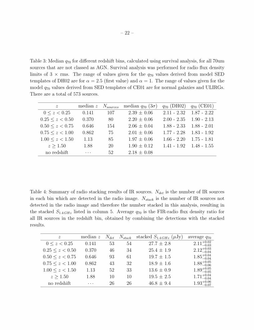
Table 3: Median q70 for different redshift bins, calculated using survival analysis, for all 70um

sources that are not classed as AGN. Survival analysis was performed for radio flux density

limits of 3 × rms. The range of values given for the q70 values derived from model SED

templates of DH02 are for α = 2.5 (first value) and α = 1. The range of values given for the

model q70 values derived from SED templates of CE01 are for normal galaxies and ULIRGs.

There are a total of 573 sources.

z median z Nsources median q70 (3σ) q70 (DH02) q70 (CE01)

0 ≤ z < 0.25 0.141 107 2.39 ± 0.06 2.11 - 2.32 1.87 - 2.22

0.25 ≤ z < 0.50 0.370 80 2.20 ± 0.06 2.00 - 2.35 1.90 - 2.13

0.50 ≤ z < 0.75 0.646 154 2.06 ± 0.04 1.88 - 2.33 1.88 - 2.01

0.75 ≤ z < 1.00 0.862 75 2.01 ± 0.06 1.77 - 2.28 1.83 - 1.92

1.00 ≤ z < 1.50 1.13 85 1.97 ± 0.06 1.66 - 2.20 1.75 - 1.81

z ≥ 1.50 1.88 20 1.90 ± 0.12 1.41 - 1.92 1.48 - 1.55

no redshift · · · 52 2.18 ± 0.08

Table 4: Summary of radio stacking results of IR sources. Ndet is the number of IR sources

in each bin which are detected in the radio image. Nstack is the number of IR sources not

detected in the radio image and therefore the number stacked in this analysis, resulting in

the stacked S1.4GHz listed in column 5. Average q70 is the FIR-radio flux density ratio for

all IR sources in the redshift bin, obtained by combining the detections with the stacked

results.

z median z Ndet Nstack stacked S1.4GHz (µJy) average q700 ≤ z < 0.25 0.141 53 54 27.7 ± 2.8 2.11+0.02

−0.03

0.25 ≤ z < 0.50 0.370 46 34 25.4 ± 1.9 2.12+0.03−0.04

0.50 ≤ z < 0.75 0.646 93 61 19.7 ± 1.5 1.85+0.04−0.04

0.75 ≤ z < 1.00 0.862 43 32 18.9 ± 1.6 1.88+0.05−0.06

1.00 ≤ z < 1.50 1.13 52 33 13.6 ± 0.9 1.89+0.05−0.05

z ≥ 1.50 1.88 10 10 19.5 ± 2.5 1.71+0.04−0.04

no redshift · · · 26 26 46.8 ± 9.4 1.93+0.06−0.07

– 23 –

Table 5: Median qTIR for different redshift bins for only sources with both 70µm and radio

detections, and are not classed as AGN. There are a total of 297 sources.

z median z Nsources median qTIR

0 ≤ z < 0.25 0.148 53 2.54 ± 0.05

0.25 ≤ z < 0.50 0.370 46 2.52 ± 0.04

0.50 ≤ z < 0.75 0.626 93 2.41 ± 0.03

0.75 ≤ z < 1.00 0.890 43 2.35 ± 0.04

1.00 ≤ z < 1.50 1.13 52 2.33 ± 0.03

z ≥ 1.50 1.91 10 2.52 ± 0.11

Table 6: Median qTIR for different redshift bins, calculated using survival analysis, for all

70µm sources that are not classed as AGN. Survival analysis was performed using L1.4GHz

calculated from radio flux density limits of 3 × rms. There are a total of 521 sources.

z median z Nsources median qTIR (3σ)

0 ≤ z < 0.25 0.141 107 2.74 ± 0.06

0.25 ≤ z < 0.50 0.370 80 2.70 ± 0.06

0.50 ≤ z < 0.75 0.646 154 2.60 ± 0.04

0.75 ≤ z < 1.00 0.862 75 2.53 ± 0.06

1.00 ≤ z < 1.50 1.13 85 2.55 ± 0.06

z ≥ 1.50 1.88 20 2.75 ± 0.12

– 24 –

Fig. 1.— The percentage completeness plotted against flux density. Our catalog is almost

100% complete at 9mJy, and 50% complete at ∼2.5mJy.

– 25 –

Fig. 2.— Histogram of the ratio of the maximum 24µm flux density over the total 24µm

flux density within a 9′′ radius. Sources with a ratio less than 0.8 were deemed deblend

candidates.

– 26 –

Fig. 3.— Number of candidate 24µm counterparts of 70µm sources as a function of position

offset. The line shows the number of matches from chance alone.

– 27 –

Fig. 4.— Histogram of 70µm fluxes. The black line is the histogram for all 617 sources,

while the red diagonally shaded histogram shows the 353 sources that have a radio detection

and the blue horizontally shaded histogram shows the 264 sources that do not have a radio

detection.

– 28 –

Fig. 5.— Histogram of all 562 sources that have redshift information. The black line is

the histogram for all sources that have redshift information while the red diagonally shaded

histogram shows sources with spectroscopic redshifts and the blue horizontally shaded his-

togram shows sources with photometric redshifts.

– 29 –

Fig. 6.— The total IR luminosity (8 – 1000 µm) as a function of redshift for all IR sources

with redshift information (562/617). Sources with spectroscopic redshifts are shown with

filled circles while sources with photometric redshifts are shown with open circles.

Fig. 7.— Sources which we classified as AGN based on radio morphology. The greyscale

image is the 70µm image and contours are the 1.4GHz image starting at 24 µJy (∼3 times

the rms) and increasing by factors of 2.

– 30 –

Fig. 8.— The ratio of 70µm flux density over 24µm flux density plotted against redshift.

Sources with no redshift information are shown at an artificial redshift of -0.05. The blue line

represents a simple modified blackbody SED model for starbursts with a dust temperature

of 30K with a mid-infrared slope of α = 2.4, while the red line represents a model for AGNs

with a dust temperature of 90K with a mid-infrared slope of 1.1 (Frayer et al. 2006). Error

bars are derived by combining in quadrature the standard errors in radio and IR fluxes.

– 31 –

Fig. 9.— The 70µm FIR-radio correlation plotted against redshift. The black points are

sources that have both 70µm and 1.4GHz detections while the blue arrows show the lower

limit of q70 for sources with no radio detection. The red open circles are data from xFLS

(Appleton et al. 2004). The black lines are expected q70 tracks derived from SED templates

for galaxies with total infrared luminosities of 109 (normal galaxies), 1011, 1012 and 1013L⊙

(ULIRGs) going from bottom to top, from Chary & Elbaz (2001) and the blue lines are

q70 tracks derived from SED templates from Dale & Helou (2002). Sources with no redshift

information are shown at an artificial redshift of -0.05. Error bars are derived by combining

in quadrature the standard errors in radio and IR fluxes.

– 32 –

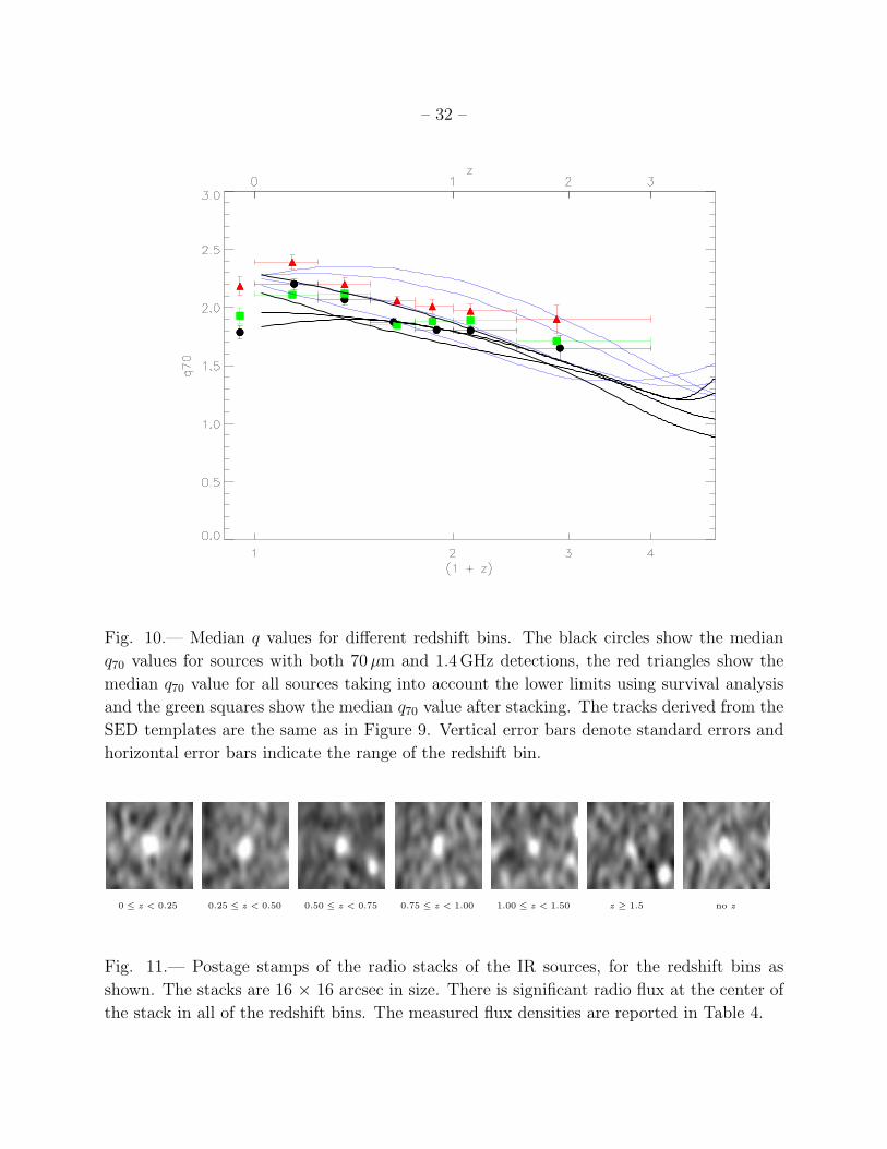
Fig. 10.— Median q values for different redshift bins. The black circles show the median

q70 values for sources with both 70µm and 1.4GHz detections, the red triangles show the

median q70 value for all sources taking into account the lower limits using survival analysis

and the green squares show the median q70 value after stacking. The tracks derived from the

SED templates are the same as in Figure 9. Vertical error bars denote standard errors and

horizontal error bars indicate the range of the redshift bin.

0 ≤ z < 0.25 0.25 ≤ z < 0.50 0.50 ≤ z < 0.75 0.75 ≤ z < 1.00 1.00 ≤ z < 1.50 z ≥ 1.5 no z

Fig. 11.— Postage stamps of the radio stacks of the IR sources, for the redshift bins as

shown. The stacks are 16 × 16 arcsec in size. There is significant radio flux at the center of

the stack in all of the redshift bins. The measured flux densities are reported in Table 4.

– 33 –

Fig. 12.— The total infrared luminosity FIR-radio correlation plotted against redshift. The

same symbol and color scheme is used as for Figure 9.

– 34 –

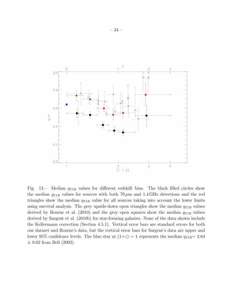
Fig. 13.— Median qTIR values for different redshift bins. The black filled circles show

the median qTIR values for sources with both 70µm and 1.4GHz detections and the red

triangles show the median qTIR value for all sources taking into account the lower limits

using survival analysis. The grey upside-down open triangles show the median qTIR values

derived by Bourne et al. (2010) and the grey open squares show the median qTIR values

derived by Sargent et al. (2010b) for star-forming galaxies. None of the data shown include

the Kellermann correction (Section 4.5.1). Vertical error bars are standard errors for both

our dataset and Bourne’s data, but the vertical error bars for Sargent’s data are upper and

lower 95% confidence levels. The blue star at (1+z) = 1 represents the median qTIR= 2.64

± 0.02 from Bell (2003).