NOAA DATA REPORT ERL PMEL-63 CTD/O MEASUREMENTS …

NOAA DATA REPORT ERL PMEL-63

CTD/O2 MEASUREMENTS COLLECTED ON A CLIMATE AND GLOBAL CHANGECRUISE (WOCE SECTIONS P14S AND P15S) DURING JANUARY–MARCH, 1996

K.E. McTaggartG.C. Johnson

Pacific Marine Environmental Laboratory7600 Sand Point Way N.E.Seattle, WA 98115-0070

September 1997

Contribution No. 1895 from NOAA/Pacific Marine Environmental Laboratory

ii

NOTICE

Mention of a commercial company or product does not constitute an endorsementby NOAA/ERL. Use of information from this publication concerning proprietaryproducts or the tests of such products for publicity or advertising purposes is notauthorized.

Contribution No. 1895 from NOAA/Pacific Marine Environmental Laboratory

__________________________________________________For sale by the National Technical Information Service, 5285 Port Royal Road

Springfield, VA 22161

iii

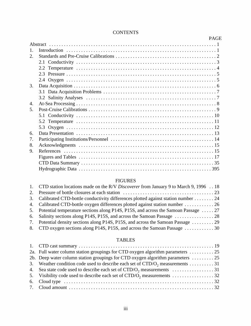
CONTENTSPAGE

Abstract . . . . . . . . . . . . . . . . . . . . . . . . . . . . . . . . . . . . . . . . . . . . . . . . . . . . . . . . . . . . . . . . . . . . 1 1. Introduction . . . . . . . . . . . . . . . . . . . . . . . . . . . . . . . . . . . . . . . . . . . . . . . . . . . . . . . . . . . . . 1 2. Standards and Pre-Cruise Calibrations. . . . . . . . . . . . . . . . . . . . . . . . . . . . . . . . . . . . . . . . . 2

2.1 Conductivity . . . . . . . . . . . . . . . . . . . . . . . . . . . . . . . . . . . . . . . . . . . . . . . . . . . . . . . . . 3 2.2 Temperature. . . . . . . . . . . . . . . . . . . . . . . . . . . . . . . . . . . . . . . . . . . . . . . . . . . . . . . . . 4 2.3 Pressure. . . . . . . . . . . . . . . . . . . . . . . . . . . . . . . . . . . . . . . . . . . . . . . . . . . . . . . . . . . . . 5 2.4 Oxygen . . . . . . . . . . . . . . . . . . . . . . . . . . . . . . . . . . . . . . . . . . . . . . . . . . . . . . . . . . . . . 5

3. Data Acquisition. . . . . . . . . . . . . . . . . . . . . . . . . . . . . . . . . . . . . . . . . . . . . . . . . . . . . . . . . . 6 3.1 Data Acquisition Problems. . . . . . . . . . . . . . . . . . . . . . . . . . . . . . . . . . . . . . . . . . . . . . 7 3.2 Salinity Analyses. . . . . . . . . . . . . . . . . . . . . . . . . . . . . . . . . . . . . . . . . . . . . . . . . . . . . 7

4. At-Sea Processing. . . . . . . . . . . . . . . . . . . . . . . . . . . . . . . . . . . . . . . . . . . . . . . . . . . . . . . . . 8 5. Post-Cruise Calibrations. . . . . . . . . . . . . . . . . . . . . . . . . . . . . . . . . . . . . . . . . . . . . . . . . . . . 9

5.1 Conductivity . . . . . . . . . . . . . . . . . . . . . . . . . . . . . . . . . . . . . . . . . . . . . . . . . . . . . . . . 10 5.2 Temperature. . . . . . . . . . . . . . . . . . . . . . . . . . . . . . . . . . . . . . . . . . . . . . . . . . . . . . . . 11 5.3 Oxygen . . . . . . . . . . . . . . . . . . . . . . . . . . . . . . . . . . . . . . . . . . . . . . . . . . . . . . . . . . . . 12

6. Data Presentation. . . . . . . . . . . . . . . . . . . . . . . . . . . . . . . . . . . . . . . . . . . . . . . . . . . . . . . . 13 7. Participating Institutions/Personnel. . . . . . . . . . . . . . . . . . . . . . . . . . . . . . . . . . . . . . . . . . 14 8. Acknowledgments. . . . . . . . . . . . . . . . . . . . . . . . . . . . . . . . . . . . . . . . . . . . . . . . . . . . . . . 15 9. References. . . . . . . . . . . . . . . . . . . . . . . . . . . . . . . . . . . . . . . . . . . . . . . . . . . . . . . . . . . . . 15

Figures and Tables. . . . . . . . . . . . . . . . . . . . . . . . . . . . . . . . . . . . . . . . . . . . . . . . . . . . . . . 17 CTD Data Summary. . . . . . . . . . . . . . . . . . . . . . . . . . . . . . . . . . . . . . . . . . . . . . . . . . . . . . 35 Hydrographic Data. . . . . . . . . . . . . . . . . . . . . . . . . . . . . . . . . . . . . . . . . . . . . . . . . . . . . .395

FIGURES1. CTD station locations made on the R/V Discoverer from January 9 to March 9, 1996 . . 18 2. Pressure of bottle closures at each station. . . . . . . . . . . . . . . . . . . . . . . . . . . . . . . . . . . . . 23 3. Calibrated CTD-bottle conductivity differences plotted against station number. . . . . . . . 24 4. Calibrated CTD-bottle oxygen differences plotted against station number. . . . . . . . . . . . 26 5. Potential temperature sections along P14S, P15S, and across the Samoan Passage. . . . . 27 6. Salinity sections along P14S, P15S, and across the Samoan Passage. . . . . . . . . . . . . . . . 28 7. Potential density sections along P14S, P15S, and across the Samoan Passage. . . . . . . . . 29 8. CTD oxygen sections along P14S, P15S, and across the Samoan Passage. . . . . . . . . . . . 30

TABLES1. CTD cast summary. . . . . . . . . . . . . . . . . . . . . . . . . . . . . . . . . . . . . . . . . . . . . . . . . . . . . . . 19 2a. Full water column station groupings for CTD oxygen algorithm parameters. . . . . . . . . . 25 2b. Deep water column station groupings for CTD oxygen algorithm parameters. . . . . . . . . 25 3. Weather condition code used to describe each set of CTD/O2 measurements. . . . . . . . . . 31 4. Sea state code used to describe each set of CTD/O2 measurements. . . . . . . . . . . . . . . . . 31 5. Visibility code used to describe each set of CTD/O2 measurements. . . . . . . . . . . . . . . . . 32 6. Cloud type . . . . . . . . . . . . . . . . . . . . . . . . . . . . . . . . . . . . . . . . . . . . . . . . . . . . . . . . . . . . . 32 7. Cloud amount. . . . . . . . . . . . . . . . . . . . . . . . . . . . . . . . . . . . . . . . . . . . . . . . . . . . . . . . . . . 32

CTD/O2 Measurements Collected on a Climate and Global Change Cruise(WOCE Sections P14S and P15S) During January–March, 1996

K.E. McTaggart and G.C. Johnson

ABSTRACT. Summaries of CTD/O2 measurements and hydrographic data acquired on a Climate andGlobal Change cruise during the austral summer of 1996 aboard the NOAA ship Discoverer arepresented. The majority of these data were collected along WOCE section P14S from 53°S, 170°E to66°S, 171°E and WOCE section P15S from 67°S, 170°W to 0°, 169°W. Also presented are datacollected along a short section across the Samoan Passage. Data acquisition and processing systems aredescribed and calibration procedures are documented. Station location, meteorological conditions,CTD/O2 summary data listings, profiles, and potential temperature-salinity diagrams are included foreach cast. Section plots of oceanographic variables and hydrographic data listings are also given.

1. IntroductionThe long-term objective of the Climate and Global Change Program is to provide reliable

predictions of climate change and associated regional implications on time scales ranging from

seasons to centuries. In support of NOAA’s Climate Program, PMEL scientists have been measuring

the growing burden of greenhouse gases in the Pacific Ocean and the overlying atmosphere since

1980. The NOAA Office of Global Programs (OGP) sponsors the Ocean Tracers and Hydrography

Program and Ocean-Atmosphere Carbon Exchange Study (OACES) to study ocean circulation,

mixing processes, and the rate at which CO2 and chlorofluorocarbons (CFCs) are taken up and

released by the oceans. Work on this cruise was cooperative with the World Ocean Circulation

Experiment (WOCE) and the Joint Global Ocean Flux Study (JGOFS). Data from this cruise will

allow quantification of the zonal currents and meridional distribution of water masses throughout

the full water column in the southwestern Pacific. Tracer measurements will be used to study the

rates of mass formation and transport processes throughout the water column.

For all sections sampled on this cruise, stations were occupied at a nominal spacing of 30 nm,

closer over steeply sloped bathymetry, and never more distant than 60 nm. Stations 1–3 were test

stations occupied to evaluate the CTD/O2 and rosette systems on the transit from Hobart, Australia

to the start of P14S. These profiles were not processed and are not included in this data report. The

cruise was broken up into two legs of roughly 1-month duration each by a port stop in Wellington,

New Zealand after station 93. Station 94 was a reoccupation of station 93 to evaluate temporal

variations that occurred during the port stop.

Full water column CTD/O2 profiles were collected at all stations. Lowered Acoustic Doppler

Current Profiler (ADCP) measurements were also collected on most casts of leg 1. In addition,

underway salinity, temperature, and CO2 measurements were taken along the cruise track. Shallow

productivity casts were made daily, and ALACE floats were deployed during the cruise. Water

samples were analyzed for a suite of natural and anthropogenic tracers including salinity, dissolved

2

oxygen, inorganic nutrients, CFCs, carbon tetrachloride, dissolved inorganic carbon, total alkalinity,

pH, pCO2, dissolved organic carbon, dissolved organic nitrogen, carbon isotopes, and oxygen

isotopes. Samples were collected from productivity casts for chlorophyll and primary productivity.

Figure 1 shows station locations. Table 1 provides a summary of cast information.

WOCE section P14S began with station 4 at 53°S, 170°E in 200 m of water on the south edge

of the Campbell Plateau and ended with station 32 at 66°S, 171°E, intersecting the zonal WHP

section S4 occupied nominally along 67°S in 1992. The section consisted of 29 stations. It sampled

the entire Antarctic Circumpolar Current between the edge of the Campbell Plateau and the crest of

the Pacific-Antarctic Ridge. At the ridge crest it explored a deep passage between the Ross Sea and

the Southwest Pacific Basin. South of the ridge crest, it entered the north side of the Ross Sea Gyre.

WOCE section P15S began with station 33 at 67°S, 170°W, again intersecting the zonal WHP

section S4 occupied nominally along 67°S in 1992. It proceeded north to station 72 at 47.5°S,

170°W, whereupon it followed a diagonal in towards the Chatham Rise until station 85 at 43.25°S,

175°E. From there it moved back away from the rise towards 170°W along a diagonal to station 104

at 36°S, 170°W. It then resumed north to station 154 at 10.5°S, 170°W, whereupon it shifted

longitudes slightly to follow the axis of the Samoan Passage until station 164 at 7.5°S, 168.75°W.

From there it continued north to station 174 at the equator, 168.75°W. Station 175 and 176 were

added to the section to improve meridional resolution in the vicinity of the Samoan Passage. From

15°S to the equator the section overlapped WHP section P15N, occupied in 1994. The section

consisted of 143 stations, discounting the duplication after the Wellington port stop. It sampled the

north end of the Ross Sea Gyre, the Antarctic Circumpolar Current, the Deep Western Boundary

Current system on both flanks of the Chatham Rise, the Subtropical Gyre, and the Tropical Regime

up to the equator.

Stations 177 to 182 were taken after the completion of P15S but prior to the final port stop in

Pago Pago, American Samoa. These profiles constitute a short, nearly zonal, section near 10°S

across the Samoan Passage. These stations were taken to investigate deep water-mass and transport

variability there.

2. Standards and Pre-Cruise CalibrationsThe CTD/O2 system is a real-time data system with the data from a Sea-Bird Electronics, Inc.

(SBE) 9plus underwater unit transmitted via a conducting cable to the SBE 11plus deck unit. The

serial data from the underwater unit is sent to the deck unit in RS-232 NRZ format using a 34560 Hz

carrier-modulated differential-phase-shift-keying (DPSK) telemetry link. The deck unit decodes the

serial data and sends it to a personal computer for display and storage in a disk file using Sea-Bird

SEASOFT software.

The SBE 911plus system transmits data from primary and auxiliary sensors in the form of

binary number equivalents of the frequency or voltage outputs from those sensors. The calculations

3

required to convert from raw data to engineering units of the parameters being measured are

performed by software, either in real-time or after the data has been stored in a disk file.

The SBE 911plus system is electrically and mechanically compatible with standard

unmodified rosette water samplers made by General Oceanics (GO), including the 1016 36-position

sampler, which was used for most stations on this cruise. An optional modem and rosette interface

allows the 911plus system to control the operation of the rosette directly without interrupting the

data from the CTD, eliminating the need for a rosette deck unit.

The SBE 9plus underwater unit uses standard modular temperature (SBE 3) and conductivity

(SBE 4) sensors which are mounted with a single clamp and “L” bracket near the lower end cap. The

conductivity cell entrance is co-planar with the tip of the temperature sensor’s protective steel sheath.

The pressure sensor is mounted inside the underwater unit main housing and is ported to outside

pressure through the oil-filled plastic capillary tube seen protruding from the main housing bottom

end cap. A compact, modular unit consisting of a centrifugal pump head and a brushless DC ball-

bearing motor contained in an aluminum underwater housing pump flushes water through sensor

tubing at a constant rate independent of the CTD’s motion. This improves dynamic performance.

Motor speed and pumping rate (3000 rpm) remain nearly constant over the entire input voltage range

of 12–18 volts DC.

The SBE 11plus deck unit is a rack-mountable interface which supplies DC power to the

underwater unit, decodes the serial data stream, formats the data under microprocessor control, and

passes the data to a companion computer. It provides access to the modem channel and control of

the rosette interface. Output data is in RS-232 (serial) format.

2.1 ConductivityThe flow-through conductivity-sensing element is a glass tube (cell) with three platinum

electrodes. The resistance measured between the center electrode and end electrode pair is

determined by the cell geometry and the specific conductance of the fluid within the cell, and

controls the output frequency of a Wien Bridge circuit. The sensor has a frequency output of

approximately 3 to 12 kHz corresponding to conductivity from 0 to 7 S/m (0 to 70 mmho/cm). The

SBE 4 has a typical accuracy/stability of ±0.0003 S/m/month; resolution of 0.00004 S/m at 24

samples per second; and 6800-meter anodized aluminum housing depth rating.

Pre-cruise sensor calibrations were performed at Sea-Bird Electronics, Inc. in Bellevue,

Washington. The following coefficients were entered into SEASOFT using software module

SEACON:

4

S/N 748 S/N 1561 S/N 1562December 14, 1995 December 14, 1995 December 14, 1995

g = –4.13299236 g = –4.09205330 g = –4.16899749h = 4.36576287e–01 h = 5.28538155e–01 h = 5.53740992e–01i = –1.39236118e–04 i = –1.56949585e–04 i = –5.94323544e–05j = 2.59599092e–05 j = 3.46776288e–05 j = 3.11836344e–05ctcor = 3.2500e–06 ctcor = 3.2500e–06 ctcor = 3.2500e–06cpcor = –9.5700e–08 cpcor = –9.5700e–08 cpcor = –9.5700e–08

Conductivity calibration certificates show an equation containing the appropriate pressure-dependent

correction term to account for the effect of hydrostatic loading (pressure) on the conductivity cell:

C (S/m) = (g + hf 2 + if 3 + jf 4) / [10 (1 + ctcor t + cpcor p)]

where g, h, i, j, ctcor, and cpcor are the calibration coefficients above, f is the instrument frequency

(kHz), t is the water temperature (C), and p is the water pressure (dbar). SEASOFT automatically

implements this equation.

2.2 TemperatureThe temperature-sensing element is a glass-coated thermistor bead, pressure-protected by a

stainless steel tube. The sensor output frequency ranges from approximately 5 to 13 kHz

corresponding to temperature from –5 to 35°C. The output frequency is inversely proportional to the

square root of the thermistor resistance which controls the output of a patented Wien Bridge circuit.

The thermistor resistance is exponentially related to temperature. The SBE 3 thermometer has a

typical accuracy/stability of ±0.004°C per year, and resolution of 0.0003°C at 24 samples per second.

The SBE 3 thermometer has a fast response time of 70 ms. Its anodized aluminum housing provides

a depth rating of 6800 m.



SEACON:

S/N 1370 S/N 2038 S/N 2037November 22, 1995 December 14, 1995 December 14, 1995

g = 4.84042876e–03 g = 4.11396861e–03 g = 4.13135090e–03h = 6.74974915e–04 h = 6.20923913e–04 h = 6.33482482e–04i = 2.38622986e–05 i = 1.98024796e–05 i = 2.11340704e–05j = 1.66698127e–06 j = 1.99224715e–06 j = 2.16252937e–06f0 = 1000.0 f0 = 1000.0 f0 = 1000.0

Temperature (ITS-90) is computed according to

5

T (°C) = 1/{g+h[ln(f 0/f )] + i[ln2(f 0/f )] + j[ln3(f 0/f )]} – 273.15

where g, h, i, j, and f 0 are the calibration coefficients above and f is the instrument frequency (kHz).

SEASOFT automatically implements this equation, and converts between ITS-90 and IPTS-68

temperature scales when selected.

2.3 PressureThe Paroscientific series 4000 Digiquartz high pressure transducer uses a quartz crystal

resonator whose frequency of oscillation varies with pressure-induced stress measuring changes in

pressure as small as 0.01 parts per million with an absolute range of 0 to 10,000 psia (0 to

6885 dbar). Also, a quartz crystal temperature signal is used to compensate for a wide range of

temperature changes. Repeatability, hysteresis, and pressure conformance are 0.005% FS. The

nominal pressure frequency (0 to full scale) is 34 to 38 kHz. The nominal temperature frequency is

172 kHz + 50 ppm/°C.



SEACON:

S/N 53960 S/N 53586April 11, 1995 October 29, 1993

c1 = –4.315048e+04 c1 = –3.920451e+04 c2 = 4.542800e–01 c2 = 6.234560e–01c3 = 1.344380e–02 c3 = 1.350570e–02d1 = 3.795200e–02 d1 = 3.894300e–02d2 = 0.0 d2 = 0.0t1 = 3.034230e+01 t1 = 3.046303e+01t2 = –1.809380e–04 t2 = –9.018862e–05t3 = 4.616150e–06 t3 = 4.528890e–06t4 = 2.084220e–09 t4 = 3.309590e–09

Pressure coefficients are first formulated into

c = c1 + c2*U + c3*U2

d = d1 + d2*U

t0 = t1 + t2*U + t3*U2 + t4*U3

where U is temperature in degrees Celsius. Then pressure is computed according to

P (psia) = c * [1 – (t02/t2)] * {1 – d[1 – (t02/t2)]}

where t is pressure period (µs). SEASOFT automatically implements this equation.

6

2.4 OxygenThe SBE 13 dissolved oxygen sensor uses a Beckman polarographic element to provide in-situ

measurements at depths up to 6800 meters. This auxiliary sensor is also included in the path of

pumped sea water. Oxygen sensors determine the dissolved oxygen concentration by counting the

number of oxygen molecules per second (flux) that diffuse through a membrane. By knowing the

flux of oxygen and the geometry of the diffusion path the concentration of oxygen can be computed.

The permeability of the membrane to oxygen is a function of temperature and ambient pressure. The

interface electronics outputs voltages proportional to membrane current (oxygen current) and

membrane temperature (oxygen temperature). Oxygen temperature is used for internal temperature

compensation. Computation of dissolved oxygen in engineering units is done in the software. The

range for dissolved oxygen is 0 to 650 µmol/kg; nominal accuracy is 4 µmol/kg; resolution is

0.4 µmol/kg. Response times are 2 s at 25°C and 5 s at 0°C.

The following oxygen calibrations were entered into SEASOFT using SEACON:

S/N 130309 September 28, 1995

m = 2.4544 e–07b = –4.6633 e–10soc = 2.6721boc = –0.0178tcor = –3.3e–02pcor = 1.5e–04tau = 2.0wt = 0.67k = 8.9224c = –6.9788

The use of these constants in linear equations of the form I = mV + b and T = kV + c will yield

sensor membrane current and temperature (with a maximum error of about 0.5°C) as a function of

sensor output voltage. These scaled values of oxygen current and oxygen temperature were carried

through the SEASOFT processing stream unaltered.

3. Data AcquisitionCTD/O2 measurements were made using one of two SBE 9plus CTDs each equipped with a

fixed pumped temperature-conductivity (TC) sensor pair. A mobile pumped TC pair with dissolved

oxygen sensor was mounted on whichever CTD was in use so that dual TC measurements and

dissolved oxygen measurements were always collected. The TC pairs were monitored for calibration

drift and shifts by examining the differences between the two pairs on each CTD and comparing

CTD salinities with bottle salinity measurements.

PMEL’s SBE 9plus CTD/O2 S/N 09P8431-0315 (sampling rate 24 Hz) was mounted in a

36-position frame and employed as the primary package. Auxiliary sensors included a lowered

7

ADCP, Metrox load cell, and Benthos altimeter. Water samples were collected using a GO 36-bottle

rosette and 10-liter Niskin bottles. The primary package was used for the majority of 182 casts.

PMEL’s SBE 9plus CTD/O2 S/N 329053-0209 (sampling rate 24 Hz) was mounted in a

24-position frame and employed as the backup package. Auxiliary sensors included a Metrox load

cell and Benthos altimeter. Water samples were collected using a SBE 32 24-bottle rosette, and

4-liter Niskin bottles. One test cast and 22 bad-weather casts were made using the smaller backup

package.

The package entered the water from the stern of the ship and was held 5–15 m beneath the

surface for 1 minute in order to activate the pump and attach tag lines for package recovery. Under

ideal conditions the package was lowered at a rate of 30 m/min to 50 m, 45 m/min to 200 m, and

60 m/min to depth. Ship heave often caused substantial variation about these mean lowering rates,

especially in the Southern Ocean. Load cell values were monitored in real time during each cast. The

position of the package relative to the bottom was monitored by the ship’s Precision Depth Recorder

(PDR) and an altimeter. A bottom depth was estimated from bathymetric charts and the PDR ran

during the bottom 1000 m of the cast. Casts were generally made to within 10 m of the bottom,

sometimes farther away in heavy weather. Figure 2 shows the depths of bottle closures during the

upcast.

Upon completion of the cast, sensors were flushed with deionized water and stored with a

dilute Triton-X solution in the plumbing. Niskin bottles were then sampled for various water

properties detailed in the introduction. Sample protocols conformed to those specified by the WOCE

Hydrographic Programme.

A SBE 11plus deck unit received the data signal from the CTD. The analog data stream was

recorded onto video cassette tape as a backup. Digitized data were forwarded to a 286-AT personal

computer equipped with SEASOFT acquisition and processing software version 4.216. Temperature,

salinity, and oxygen profiles were displayed in real time. Raw data files were transferred to a 486

personal computer using Laplink version 3 and backed up to optical disk.

3.1 Data Acquisition ProblemsSome time was lost at the beginning of leg 1 owing to level-wind problems on the primary

winch. The sea cable was retensioned on the drum at sea by removing the CTD/rosette package,

attaching a weight to the cable, and spooling the full length of cable behind the ship while underway

to within the last full wrap on the drum. Level-wind problems were much reduced after this

procedure.

No useful data from the secondary TC pair and dissolved oxygen sensor were collected during

station 12 owing to biological fouling of the mobile sensors. Data from the primary TC pair were

processed for station 12, as well as for stations 69, 78, 79, 128, 130, 131, and 159 owing to noise.

No oxygen data are available for stations 132, 133, 134, and 144 during which problems with the

dissolved oxygen sensor were being diagnosed and repaired.

8

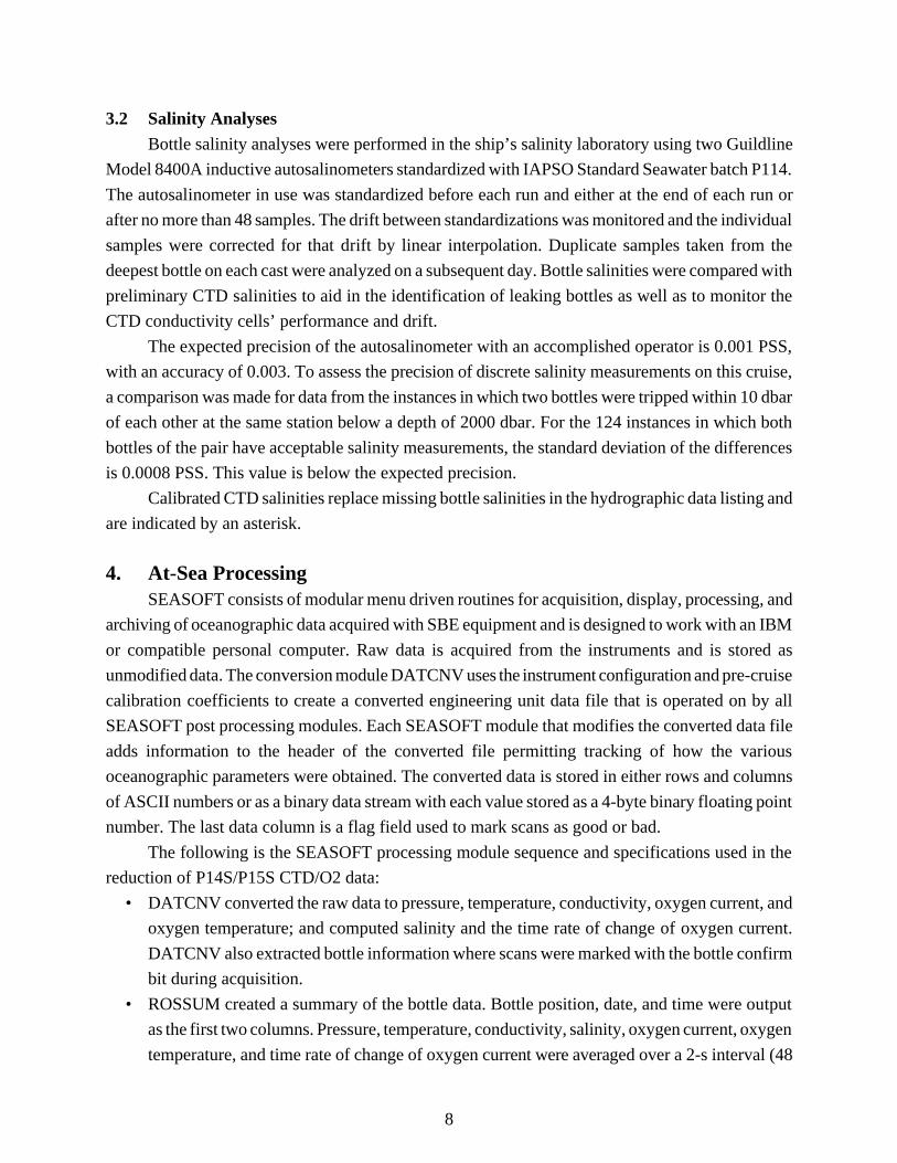
3.2 Salinity AnalysesBottle salinity analyses were performed in the ship’s salinity laboratory using two Guildline

Model 8400A inductive autosalinometers standardized with IAPSO Standard Seawater batch P114.

The autosalinometer in use was standardized before each run and either at the end of each run or

after no more than 48 samples. The drift between standardizations was monitored and the individual

samples were corrected for that drift by linear interpolation. Duplicate samples taken from the

deepest bottle on each cast were analyzed on a subsequent day. Bottle salinities were compared with

preliminary CTD salinities to aid in the identification of leaking bottles as well as to monitor the

CTD conductivity cells’ performance and drift.

The expected precision of the autosalinometer with an accomplished operator is 0.001 PSS,

with an accuracy of 0.003. To assess the precision of discrete salinity measurements on this cruise,

a comparison was made for data from the instances in which two bottles were tripped within 10 dbar

of each other at the same station below a depth of 2000 dbar. For the 124 instances in which both

bottles of the pair have acceptable salinity measurements, the standard deviation of the differences

is 0.0008 PSS. This value is below the expected precision.

Calibrated CTD salinities replace missing bottle salinities in the hydrographic data listing and

are indicated by an asterisk.

4. At-Sea ProcessingSEASOFT consists of modular menu driven routines for acquisition, display, processing, and

archiving of oceanographic data acquired with SBE equipment and is designed to work with an IBM

or compatible personal computer. Raw data is acquired from the instruments and is stored as

unmodified data. The conversion module DATCNV uses the instrument configuration and pre-cruise

calibration coefficients to create a converted engineering unit data file that is operated on by all

SEASOFT post processing modules. Each SEASOFT module that modifies the converted data file

adds information to the header of the converted file permitting tracking of how the various

oceanographic parameters were obtained. The converted data is stored in either rows and columns

of ASCII numbers or as a binary data stream with each value stored as a 4-byte binary floating point

number. The last data column is a flag field used to mark scans as good or bad.

The following is the SEASOFT processing module sequence and specifications used in the

reduction of P14S/P15S CTD/O2 data:

• DATCNV converted the raw data to pressure, temperature, conductivity, oxygen current, and

oxygen temperature; and computed salinity and the time rate of change of oxygen current.

DATCNV also extracted bottle information where scans were marked with the bottle confirm

bit during acquisition.

• ROSSUM created a summary of the bottle data. Bottle position, date, and time were output

as the first two columns. Pressure, temperature, conductivity, salinity, oxygen current, oxygen

temperature, and time rate of change of oxygen current were averaged over a 2-s interval (48

9

scans). For the primary package, the time interval was from 5 to 3 s prior to the confirm bit

in order to avoid spikes in conductivity and oxygen current owing to minor incompatibilities

between the SBE 911plus CTD/O2 system and GO 1016 rosette. Bottle data from the backup

package were averaged from 1 s prior to the confirm bit to 1 s after the confirm bit in the data

stream. ROSSUM computed CTD oxygen, potential temperature, and sigma-theta.

• WILDEDIT marked extreme outliers in the data files. The first pass of WILDEDIT obtained

an accurate estimate of the true standard deviation of the data. The data were read in blocks

of 200 scans. Data greater than two standard deviations were flagged. The second pass

computed a standard deviation over the same 200 scans excluding the flagged values. Values

greater than 16 standard deviations were marked bad.

• SPLIT removed decreasing pressure records from the data files, leaving only the downcast.

• FILTER performed a low pass filter on pressure with a time constant of 0.15 s. In order to

produce zero phase (no time shift) the filter first runs forward through the file and then runs

backwards through the file.

• ALIGNCTD aligned conductivity in time relative to pressure to ensure that all calculations

were made using measurements from the same parcel of water. Conductivity for the primary

sensor on the 36-bottle package was advanced by –0.020 s. Conductivity for the primary

sensor on the 24-bottle package was advanced by –0.010 s. Conductivity for the secondary,

mobile sensor on either package was advanced 0.055 s.

• CELLTM used a recursive filter to remove conductivity cell thermal mass effects from the

measured conductivity. For C748 with an epoxy coating, the thermal anomaly amplitude

(alpha = 0.03) and the time constant (1/beta = 9.0) were higher than for C1561 and C1562 with

no coating (alpha = 0.02, 1/beta = 7.0).

• DERIVE was used to compute fall rate (m/s) with a time window size for fall rate and

acceleration of 2.0 seconds.

• LOOPEDIT marked scans where the CTD was moving less than the minimum velocity of

0.25 m/s or traveling backwards due to ship heave.

• BINAVG averaged the data into 1-dbar pressure bins starting at 1 dbar with no surface bin.

The center value of the first bin was set equal to the bin size. The bin minimum and maximum

values are the center value ± half the bin size. Scans with pressures greater than the minimum

and less than or equal to the maximum were averaged. Scans were interpolated so that a data

record exists every decibar.

• STRIP removed scan number and fall rate from the data files.

• TRANS converted the data file format from binary to ASCII.

5. Post-Cruise CalibrationsPost-cruise sensor calibrations were done at Sea-Bird Electronics, Inc. during May 1996.

Mobile, secondary sensor pair T1370 and C748 were selected for final data reduction for all stations

10

except 12, 69, 128, 130, 131, and 159. Post-cruise calibrations showed T1370 to have drifted by

0.43e–03°C over the 3.2 months between calibrations. Station 12 data are from sensors T2037 and

C1562. Post-cruise calibrations showed T2037 to have drifted by –0.28e–03°C over the 3.2 months

between calibrations. The remaining station data are from sensors T2038 and C1561. Post-cruise

calibrations showed T2038 to have drifted by 0.11e–03°C over the 3.3 months between calibrations.

5.1 ConductivitySEASOFT module ALIGNCTD was used to align conductivity measurements in time relative

to pressure. Measurements can be misaligned due to the inherent time delay of the sensor response,

the water transit time delay in the pumped plumbing line, and the sensors being physically

misaligned in depth. Because SBE 3 temperature response is fast (0.06 s), it is not necessary to

advance temperature relative to pressure. When measurements are properly aligned, salinity spiking

and density errors are minimized.

For a SBE 9 CTD with ducted TC sensors and a 3000 rpm pump the typical net advance of

conductivity relative to temperature is 0.073 s. The SBE 11 deck unit advances primary conductivity

by 0.073 s but does not advance secondary conductivity. Therefore the alignment of C748

conductivity data, which was from the secondary sensor channel (except for stations 78 and 79), was

much larger, typically 0.06 s versus coming from a primary sensor channel, typically 0.02 s.

Conductivity slope and bias, along with a linear pressure term (modified beta), were computed

by a least-squares minimization of CTD and bottle conductivity differences. The function minimized

was

BC – m * CC – b – beta * CP

where BC is bottle conductivity (S/m), CC is pre-cruise calibrated CTD conductivity (S/m), CP is

the CTD pressure (dbar), m is the conductivity slope, b is the bias (S/m), and beta is a linear pressure

term (S/m/dbar). The final CTD conductivity (S/m) is

m * CC + b + beta * CP

The slope term m is a fourth-order polynomial function of station number to allow the entire cruise

to be fit at once with a smoothly-varying station-dependent slope correction. For sensors C748 and

C1561 a series of fits were made, each fit throwing out bottle values for locations having a residual

between CTD and bottle conductivity greater than three standard deviations. This procedure was

repeated with the remaining bottle values until no more bottle values were thrown out.

For C748, the slope correction ranged from 1.0000501 to 1.0001274, the bias applied was

–7.5e–04 S/m, and the beta term was –9.01e–09 S/m/dbar. Of 5680 bottles, the percentage of bottles

retained in the fit was 85.2 with a standard deviation of CTD versus bottle conductivity differences

11

of 9.88e–05 S/m. For C1561, the slope correction ranged from 1.0001481 to 1.0002849, the bias

applied was –3.8e–04 S/m, and the beta term was –3.16e–09 S/m/dbar. Of 5118 bottles, the

percentage of bottles retained in the fit was 88.1 with a standard deviation of 9.93e–05 S/m.

For station 12, station 13 calibrated secondary salinity data was used as a reference. A slope,

bias, and pressure correction was determined that matched station 13 uncalibrated primary salinity

(C1562, T2037) to station 13 calibrated secondary salinity (C748, T1370). These coefficients

(slope = 1.004, bias = –0.0011 S/m, beta = –2.49e–08 S/m/dbar) were used to calibrate station 12

primary salinity (C1562, T2037).

CTD-bottle conductivity differences are plotted against station number to show the stability

of the calibrated CTD conductivities relative to the bottle conductivities (Fig. 3, upper panel).

CTD-bottle conductivity differences are plotted against pressure to show the tight fit below 500 m

and the increasing scatter above 500 m (Fig. 3, lower panel).

5.2 TemperatureAdjustments were made to the bias of the thermistors as deviations from the pre-cruise

calibrations on a station-by-station basis. These deviations were obtained from a linear fit of the

pre-cruise and post-cruise temperature residuals from the pre-cruise calibration versus time.

A pressure correction was then applied to each sensor such that

CT = CT * pcor * CP

where CT is CTD temperature (°C) with the bias adjustment, pcor is the pressure correction (dbar)

for each sensor, and CP is CTD pressure (dbar).

pcor1370 = –2.6e–03/9000 dbar = –2.8889e–007 1/dbar

pcor2037 = –2.3e–03/9000 dbar = –2.5556e–007 1/dbar

pcor2038 = –1.7e–03/9000 dbar = –1.8889e–007 1/dbar

Also, a uniform correction was applied for heating of the thermistor owing to viscous effects.

All the thermistors were biased high by this effect and were adjusted down accordingly. An

adjustment of 0.6e–03°C results in errors of no more than ±0.15°C from this effect for the full range

of oceanographic temperature and salinity.

Post-cruise temperature and conductivity calibrations were applied to all sensor pairs using

PMEL program CALCTD (STA12CAL for station 12). Surface values were filled using PMEL

program FILLSFC. FILLSFC copied the first good value of salinity and potential temperature back

to the surface and then back-calculated temperature and conductivity. Primary and secondary sensor

differences were examined. Data from the secondary sensor pair (T1370/C748) were chosen for all

stations except 12, 69, 78, 79, 128, 130, 131, and 159. Primary sensor data chosen for these 8

12

stations were within .001 PSS of the secondary sensor data of the surrounding stations. All profiles

were despiked and data linearly interpolated using PMEL program DESPIKE.

Package slowdowns and reversals owing to ships heave can move mixed water in tow to in

front of the CTD sensors and obscure measurements. In addition to SEASOFT module LOOPEDIT

(see section 4), PMEL program DELOOP computed values of density locally referenced between

every 1 dbar of pressure to compute N2 = (–g/rho)(drho/dz) and linearly interpolated over those

records where N2 � –1.0e–05 s–2.

Post-cruise calibrations were applied to CTD data associated with bottle data using PMEL

program CALMSTR. CALMSTR also amended WOCE quality flags associated with CTD and

bottle salinities. Eighteen CTD salinities were flagged as bad during station 78 likely owing to

clogged plumbing of the primary sensors during the upcast. Of the 5640 bottle salinities, 0.33% were

flagged as bad and 2.68% were flagged as questionable.

5.3 OxygenIn situ oxygen samples collected during CTD/O2 profiles are used for post-measurement

calibration. Calibrated CTD/O2 data associated with bottle data were merged with bottle oxygen data

flagged as “good.” Because the dissolved oxygen sensor has an obvious hysteresis, PMEL program

OXDWNP replaced up-profile water sample data with corresponding down-profile CTD/O2 data at

common pressure levels. The time rate of change of oxygen current was computed using 2-s

intervals in SEASOFT and smoothed using a median filter of width 5 dbar prior to OXDWNP.

Oxygen saturation values were computed according to Benson and Krause (1984) in units of

µmol/kg.

The algorithm used for converting oxygen sensor current and probe temperature measurements

to oxygen as described by Owens and Millard (1985) requires a non-linear least squares regression

technique in order to determine the best fit coefficients of the model for oxygen sensor behavior to

the water sample observations. WHOI program OXFITMR uses Numerical Recipes (Press et al.,

1986) Fortran routines MRQMIN, MRQCOF, GAUSSJ, and COVSRT to perform non-linear least

squares regression using the Levenberg-Marquardt method. A Fortran subroutine FOXY describes

the oxygen model with the derivatives of the model with respect to six coefficients in the following

order: oxygen current slope, temperature correction, pressure correction, weight, oxygen current bias,

and oxygen current lag.

Program OXFITMR reads the data for a group of stations. The data are edited to remove

spurious points where values are less than zero or greater than 1.2 times the saturation value. The

routine varies the six (or fewer) parameters of the model in such a way as to produce the minimum

sum of squares in the difference between the calibration oxygens and the computed values.

Individual differences between the calibration oxygens and the computed oxygen values (residuals)

are then compared with the standard deviation of the residuals. Any residual exceeding an edit factor

of 2.8 standard deviations is rejected. A factor of 2.8 will have a 0.5% chance of rejecting a valid

13

oxygen value for a normally distributed set of residuals. The iterative fitting process is continued

until none of the data fail the edit criteria. The best fit to the oxygen probe model coefficients is then

determined. Coefficients were applied by PMEL program CALOX2W and CTD oxygen was

computed using subroutine OXY6W.

By plotting the oxygen residuals versus station, appropriate station groupings for further

refinements of fitting are obtained by looking for abrupt station-to-station changes in the residuals.

For each grouping, two sets of coefficients were determined, one fitting all the bottles and a second

fitting only bottles deeper than just above the median bottle oxygen minimum. Sometimes it was

necessary to fix values of some oxygen algorithm parameters to keep those parameters within a

reasonable range (noted by asterisks in Table 2). Final coefficients were applied to downcast data

using PMEL program OXYCALC; and to bottle data using OXYCALB. The two sets of coefficients

were blended at the oxygen minimum using a set of hyperbolic tangent functions with 250-dbar

decay scales.

CTD oxygen values were despiked using PMEL program CLEANOX. Bad CTD oxygen data

were flagged for all of station 12 owing to clogged plumbing, parts of stations 127–131 where the

dissolved oxygen module failed in the deep water (the dissolved oxygen module was replaced prior

to station 135), and stations 177–182 above 2850 dbar where no shallow bottle data were available

to calibrate the sensor.

CTD-bottle oxygen differences are plotted against station number to show the stability of the

calibrated CTD oxygens relative to the bottle oxygens (Fig. 4, upper panel). Note that the residuals

are well below the nominal accuracy quoted for the oxygen sensor. CTD-bottle oxygen differences

are plotted against pressure to show the tight fit below 1200 m and the increasing scatter above

1200 m (Fig. 4, lower panel).

PMEL program P15_EPIC converted finalized CTD/O2 data files into EPIC format (Soreide,

1995), and computed ITS-90 temperature, ITS-90 potential temperature, and dynamic height. EPIC

datafiles contain a WOCE quality flag parameter associated with pressure, temperature, CTD

salinity, and CTD oxygen. Quality flag definitions can be found in the WOCE Operations Manual

(1994).

6. Data PresentationThe final calibrated data in EPIC format were used to produce the plots and listings which

follow. The majority of the plots were produced using Plot Plus Scientific Graphics System (Denbo,

1992). Vertical sections of potential temperature, CTD salinity, potential density, and CTD oxygen

are contoured with pressure as the vertical axis and latitude as the horizontal axis (Figs. 5–8).

Nominal vertical exaggerations are 1000:1 below 1000 dbar (lower panels) and 2500:1 above

1000 dbar (upper panels). Plots and summary listings of the CTD/O2 data follow for each cast.

Tables 3–7 define the abbreviations and units used in the CTD/O2 data summary listings.

Hydrographic bottle data at discrete depths are listed in the final section.

14

The hydrographic listings presented include two-digit WOCE quality flags. The numeric digits

are associated with bottle salinity and bottle oxygen. Quality flag definitions can be found in the

WOCE Operations Manual (1994).

7. Participating Institutions/Personnel

NOAA Pacific Marine Environmental Laboratory (PMEL)NOAA Atlantic Oceanographic and Meterological Laboratory (AOML)Bermuda Biological Station for Research (BBSR)Monterey Bay Aquarium Research Institute (MBARI)Scripps Institution of Oceanography (SIO)University of Tennessee (UT)University of Hawaii (UH)University of Washington (UW)University of Miami (UM)University of South Florida (USF)University of Charleston, South Carolina (UCSC)

Measurement Principal Investigator Institution

CTD/O2, salinity G. Johnson PMELChlorofluorocarbons (CFCs) J. Bullister PMELTotal CO2 (DIC), pCO2 R. Feely PMELC-14 (AMS radiocarbon), C-13 P. Quay UWNutrients C. Mordy PMEL

Z. Zhang AOMLDissolved Oxygen J. Bullister PMELTotal alkalinity F. Millero UMpH R. Byrne USFUnderway pH/DIC A. Dickson SIODOC/DON D. Hansell BBSRADCP P. Hacker/E. Firing UHALACE floats R. Davis SIOPrimary productivity J. DiTullio UCSC

W. Smith UTUnderway chlorophyll F. Chavez MBARI

Leg 1 Leg 2

John Bullister, PMEL Chief Scientist xGreg Johnson, PMEL Co-Chief Scientist xDick Feely, PMEL Chief Scientist xMarilyn Roberts, PMEL Co-Chief Scientist xKristy McTaggart, PMEL CTD x xNorge Larson, Sea-Bird CTD xJohn Love, IOS CTD xJim Richman, OSU CTD xGregg Thomas, AOML salinity x xDave Wisegarver, PMEL CFC x xCraig Neill, PMEL CFC x x

15

Wenlin Huang, PMEL CFC xKirk Hargreaves, PMEL oxygen x xCarol Stewart, IOS oxygen/CFC x xCalvin Mordy, PMEL nutrients x xZia-Zhong Zhang, AOML nutrients x xTom Lantry, AOML DIC x xMarilyn Roberts, PMEL DIC xKim Currie, IOS DIC xCathy Cosca, PMEL underway pCO2 xDana Greeley, PMEL pCO2 x xHua Chen, AOML pCO2 xRhonda Kelly, BBSR pCO2 xJamie Goen, RSMAS alkalinity x xDavid Purkinson, RSMAS alkalinity xMary Roche, RSMAS alkalinity xChris Edwards, RSMAS alkalinity xXiarong Zhu, RSMAS alkalinity xSean McElligott, USF pH x xWensheng Yao, USF pH x xJohan Schijf, USF pH xXeuwu Liu, USF pH xEric Firing, UH ADCP xSusan Becker, BBSR DOC x xRachel Parsons, BBSR DOC x xBrian Kleinhaus, UW C-13, C-14 xTanya Westby, UW C-13, C-14 xKendra Daly, UTK productivity x xDavid Jones, UCSC productivity x xPeter Walz, MBARI productivity xTim Pennington, MBARI productivity x

8. AcknowledgmentsThe assistance of the officers, crew, and survey department of the NOAA ship Discoverer is

gratefully acknowledged. Funds for the CTD/O2 program were provided to PMEL by the Climate

and Global Change program under NOAA’s Office of Global Programs.

9. ReferencesBenson, B.B., and D. Krausse Jr. (1984): The concentration and isotopic fractionation of oxygen

dissolved in freshwater and seawater in equilibrium with the atmosphere. Limnol. Oceanogr.,

29, 620–632.

Denbo, D.W. (1992): PPLUS Graphics, P.O. Box 4, Sequim, WA, 98382.

Owens, W.B., and R.C. Millard Jr. (1985): A new algorithm for CTD oxygen calibration. J. Phys.

Oceanogr., 15, 621–631.

Press, W., B. Flannery, S. Teukolsky, and W. Vetterling (1986): Numerical Recipes: The Art of

Scientific Computing. Cambridge University Press, 818 pp.

16

Seasoft CTD Acquisition Software Manual (1994): Sea-Bird Electronics, Inc., 1808 136th Place NE,

Bellevue, Washington, 98005.

Soreide, N.N., M.L. Schall, W.H. Zhu, D.W. Denbo, and D.C. McClurg (1995): EPIC: An

oceanographic data management, display and analysis system. Proceedings, 11th International

Conference on Interactive Information and Processing Systems for Meteorology,

Oceanography, and Hydrology, January 15–20, 1995, Dallas, TX, 316–321.

WOCE Operations Manual (1994): Volume 3: The Observational Programme, Section 3.1: WOCE

Hydrographic Programme, Part 3.1.2: Requirements for WHP Data Reporting. WHP Office

Report 90-1, WOCE Report No. 67/91, Woods Hole, MA, 02543.

17

FIGURES AND TABLES

18

Fig. 1. CTD station locations made on the R/V Discoverer from January 9 to March 9, 1996.

19

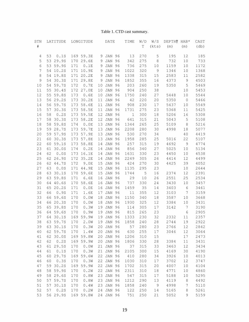
Table 1. CTD cast summary.

STN LATITUDE LONGITUDE DATE TIME W/D W/S DEPTH + HAB* CAST # T (kts) (m) (m) (db)

4 53 0.1S 169 59.3E 9 JAN 96 13 270 5 195 12 185 5 53 29.9S 170 29.6E 9 JAN 96 342 275 8 732 10 733 6 53 59.9S 171 0.1E 9 JAN 96 736 275 10 1159 10 1172 7 54 10.2S 171 10.9E 9 JAN 96 1022 320 9 1346 10 1368 8 54 19.8S 171 20.2E 9 JAN 96 1338 315 15 2583 11 2582 9 54 30.3S 171 29.8E 9 JAN 96 1852 355 16 4373 9 4503 10 54 59.7S 172 0.7E 10 JAN 96 203 260 19 5350 5 5469 11 55 30.4S 172 27.0E 10 JAN 96 904 250 38 10 5453 12 55 59.8S 173 0.6E 10 JAN 96 1750 240 27 5448 10 5544 13 56 29.2S 173 30.2E 11 JAN 96 42 220 20 5350 0 5466 14 56 59.7S 173 58.6E 11 JAN 96 908 230 17 5437 10 5549 15 57 30.3S 173 58.5E 11 JAN 96 1731 275 23 5368 11 5425 16 58 0.2S 173 59.5E 12 JAN 96 1 300 18 5206 16 5308 17 58 30.3S 173 58.2E 12 JAN 96 641 315 21 5043 5 5108 18 58 59.8S 174 0.0E 13 JAN 96 1344 265 25 5109 8 5216 19 59 28.7S 173 59.7E 13 JAN 96 2208 280 30 4998 18 5077 20 59 57.9S 173 57.9E 13 JAN 96 530 270 34 40 4419 21 60 30.3S 173 57.8E 13 JAN 96 1958 285 25 5016 22 5107 22 60 59.1S 173 58.8E 14 JAN 96 257 315 19 4692 9 4774 23 61 30.0S 174 0.2E 14 JAN 96 856 340 27 5025 10 5134 24 62 0.0S 173 16.1E 14 JAN 96 1631 330 23 4450 10 4538 25 62 26.9S 172 35.2E 14 JAN 96 2249 305 26 4414 12 4499 26 62 44.7S 172 9.0E 15 JAN 96 424 270 30 4425 39 4052 27 63 0.0S 171 44.9E 15 JAN 96 1135 295 23 10 2644 28 63 30.1S 170 59.6E 15 JAN 96 1744 5 16 2374 12 2391 29 63 59.8S 171 6.6E 16 JAN 96 29 10 26 2551 25 2534 30 64 40.6S 170 58.6E 16 JAN 96 737 330 24 3430 10 3457 31 65 20.2S 171 0.0E 16 JAN 96 1459 35 14 3403 6 3461 32 66 0.9S 171 1.6E 17 JAN 96 11 355 12 3103 7 3159 33 66 59.6S 170 0.0W 18 JAN 96 1150 340 18 3587 10 3668 34 66 20.3S 170 0.0W 18 JAN 96 1930 325 12 3384 10 3431 35 65 39.8S 170 0.3W 19 JAN 96 114 305 17 3142 7 3190 36 64 59.6S 170 0.9W 19 JAN 96 815 265 23 6 2905 37 64 30.1S 169 59.9W 19 JAN 96 1333 230 32 2332 11 2357 38 63 59.7S 170 2.0W 19 JAN 96 1858 240 28 2744 19 2922 39 63 30.1S 170 0.3W 20 JAN 96 57 280 23 2766 12 2842 40 62 59.7S 170 1.4W 20 JAN 96 630 255 17 3046 12 3064 41 62 30.0S 169 59.8W 20 JAN 96 1206 310 15 17 2473 42 62 0.2S 169 59.9W 20 JAN 96 1806 330 28 3384 11 3431 43 61 29.5S 170 0.0W 21 JAN 96 37 315 33 3463 12 3434 44 61 0.1S 170 0.3W 21 JAN 96 2105 300 15 4169 30 4190 45 60 29.7S 169 59.6W 22 JAN 96 410 280 34 3926 10 4013 46 60 0.3S 170 0.3W 22 JAN 96 1030 310 17 3702 12 3747 47 59 30.2S 169 59.9W 22 JAN 96 1702 315 20 4007 10 4104 48 58 59.9S 170 0.2W 22 JAN 96 2311 310 18 4771 10 4860 49 58 29.6S 170 0.8W 23 JAN 96 547 315 17 5188 10 5295 50 57 59.7S 170 0.8W 23 JAN 96 1212 290 13 4119 8 4492 51 57 30.1S 170 0.4W 23 JAN 96 1858 240 9 4998 7 5110 52 57 0.2S 170 0.2W 24 JAN 96 122 250 14 5165 8 5261 53 56 29.9S 169 59.8W 24 JAN 96 751 250 21 5052 9 5159

20

Table 1. (continued).


54 56 0.0S 170 1.8W 24 JAN 96 1352 220 20 5157 7 5236 55 55 29.9S 170 0.0W 24 JAN 96 2050 240 5 4945 9 5049 56 54 59.8S 170 0.0W 25 JAN 96 307 285 11 4812 7 4916 57 54 29.4S 170 0.1W 25 JAN 96 900 285 13 4811 3 4929 58 54 0.1S 169 59.3W 25 JAN 96 1545 290 16 5009 8 5138 59 53 39.9S 169 59.4W 25 JAN 96 2122 270 17 5131 5 5253 60 53 19.9S 169 59.6W 26 JAN 96 320 280 22 5286 8 5459 61 53 0.0S 170 0.5W 26 JAN 96 925 275 22 5193 9 5298 62 52 29.9S 170 1.8W 26 JAN 96 1643 270 27 5070 7 5173 63 52 0.1S 170 7.8W 26 JAN 96 2325 275 26 4970 10 5067 64 51 30.0S 170 0.2W 27 JAN 96 606 270 26 4754 20 4876 65 51 0.2S 170 0.4W 27 JAN 96 1221 250 20 5249 12 5321 66 50 29.9S 169 59.6W 27 JAN 96 1937 220 10 5052 15 5129 67 50 0.4S 169 59.9W 28 JAN 96 225 210 11 5361 8 5479 68 49 30.3S 170 0.9W 28 JAN 96 917 265 15 5217 15 5337 69 48 59.6S 169 59.4W 28 JAN 96 1633 270 18 5253 10 5340 70 48 30.0S 170 0.2W 28 JAN 96 2248 310 10 5303 5 5409 71 47 59.8S 170 0.3W 29 JAN 96 531 340 10 5293 10 5400 72 47 30.3S 169 59.8W 29 JAN 96 1148 45 13 5309 5 5474 73 47 6.5S 170 27.7W 29 JAN 96 1902 70 6 5391 8 5500 74 46 43.4S 170 54.7W 30 JAN 96 124 45 6 5292 9 5387 75 46 20.0S 171 22.2W 30 JAN 96 743 50 10 5101 8 5196 76 45 57.0S 171 49.5W 30 JAN 96 1446 100 15 5156 9 5250 77 45 33.6S 172 16.7W 30 JAN 96 2127 110 9 4968 7 5057 78 45 10.6S 172 44.2W 31 JAN 96 443 180 10 4660 10 4738 79 44 50.1S 173 8.2W 31 JAN 96 1035 230 15 3832 10 3869 80 44 31.8S 173 29.4W 31 JAN 96 1707 230 16 3397 10 3452 81 44 19.2S 173 44.7W 31 JAN 96 2119 225 10 3077 9 3115 82 44 9.4S 173 56.3W 1 FEB 96 106 280 5 1897 10 1911 83 43 50.9S 174 17.7W 1 FEB 96 434 250 11 946 10 959 84 43 38.8S 174 32.2W 1 FEB 96 710 0 0 790 10 789 85 43 15.2S 174 59.9W 1 FEB 96 1023 280 9 788 12 785 86 42 55.9S 174 47.2W 1 FEB 96 1328 270 5 1054 10 1055 87 42 44.8S 174 39.3W 1 FEB 96 1627 300 4 1581 9 1595 88 42 24.1S 174 24.4W 1 FEB 96 2014 315 7 2654 10 2677 89 42 10.1S 174 15.0W 2 FEB 96 6 350 10 2862 7 2889 90 41 42.8S 173 56.5W 2 FEB 96 520 330 12 3118 6 3162 91 41 16.0S 173 38.7W 2 FEB 96 1014 325 12 3319 6 3353 92 40 49.5S 173 19.5W 2 FEB 96 1545 330 14 4169 6 4239 93 40 23.6S 173 2.0W 2 FEB 96 2056 345 18 4574 9 4652 94 40 23.5S 173 1.7W 13 FEB 96 2049 130 15 4574 4 4658 95 39 57.7S 172 42.2W 14 FEB 96 326 150 22 4738 8 4823 96 39 31.0S 172 25.2W 14 FEB 96 937 190 23 4761 8 4848 97 39 4.3S 172 7.7W 14 FEB 96 1612 160 18 4835 10 4929 98 38 37.8S 171 48.6W 14 FEB 96 2202 140 12 4914 10 5003 99 38 11.4S 171 30.2W 15 FEB 96 423 140 8 4932 10 5031 100 37 45.8S 171 12.0W 15 FEB 96 1033 130 14 4997 7 5119 101 37 18.6S 170 53.7W 15 FEB 96 1727 145 14 5130 5 5230 102 36 52.3S 170 37.0W 15 FEB 96 2306 210 12 5278 6 5384 103 36 27.0S 170 17.2W 16 FEB 96 513 220 15 5122 8 5219

21



104 36 0.2S 170 0.3W 16 FEB 96 1135 200 19 5069 8 5156 105 35 40.3S 170 0.9W 16 FEB 96 1727 205 24 4292 5 4329 106 35 20.0S 170 0.1W 16 FEB 96 2233 170 21 4895 7 4981 107 35 0.5S 169 59.6W 17 FEB 96 415 140 19 5250 5 5348 108 34 30.3S 170 0.2W 17 FEB 96 1137 160 20 5487 6 5591 109 33 59.8S 170 0.0W 17 FEB 96 1849 150 16 5533 6 5640 110 33 29.9S 170 0.1W 18 FEB 96 119 150 10 5416 6 5509 111 33 0.1S 170 0.1W 18 FEB 96 736 115 10 5582 10 5677 112 32 30.1S 170 0.1W 18 FEB 96 1404 115 8 5533 7 5651 113 31 59.8S 169 59.8W 18 FEB 96 2055 140 6 5677 7 5790 114 31 30.0S 169 59.3W 19 FEB 96 330 90 7 5526 8 5645 115 31 0.4S 169 59.7W 19 FEB 96 951 80 15 5606 7 5725 116 30 30.3S 169 59.8W 19 FEB 96 1640 90 14 5537 9 5640 117 30 0.2S 169 59.8W 19 FEB 96 2259 80 12 5413 7 5514 118 29 30.2S 169 59.8W 20 FEB 96 503 90 15 5148 12 5190 119 29 0.8S 169 59.9W 20 FEB 96 1113 70 18 5596 15 5684 120 28 30.5S 169 59.8W 20 FEB 96 1809 90 10 5459 9 5555 121 28 0.3S 169 59.6W 21 FEB 96 10 90 13 4907 10 4966 122 27 30.1S 170 0.1W 21 FEB 96 600 100 20 5349 7 5485 123 27 0.3S 169 59.5W 21 FEB 96 1202 95 13 5241 7 5331 124 26 29.7S 169 59.4W 21 FEB 96 1906 110 24 5613 8 5710 125 26 0.3S 169 59.7W 22 FEB 96 321 100 20 5601 9 5695 126 25 30.0S 170 0.0W 22 FEB 96 1005 105 17 5833 9 5944 127 25 0.1S 169 59.9W 22 FEB 96 1734 100 20 5640 3 5818 128 24 30.0S 170 0.1W 23 FEB 96 16 90 16 5650 10 5757 129 23 59.8S 170 0.1W 23 FEB 96 720 80 16 5678 10 5780 130 23 30.1S 170 0.1W 23 FEB 96 1404 100 18 5666 7 5781 131 22 59.8S 169 59.7W 23 FEB 96 2139 120 9 5691 9 5799 132 22 30.0S 169 59.9W 24 FEB 96 448 120 13 5649 7 5752 133 22 0.0S 169 59.9W 24 FEB 96 1127 160 12 5626 8 5731 134 21 30.4S 170 0.1W 24 FEB 96 1837 150 7 5421 6 5514 135 20 59.7S 169 59.6W 25 FEB 96 107 160 5 5461 4 5566 136 20 29.9S 170 0.1W 25 FEB 96 739 175 5 5598 40 5722 137 20 0.0S 170 0.1W 25 FEB 96 1354 170 6 5315 7 5429 138 19 29.9S 170 0.1W 25 FEB 96 2023 80 4 4904 8 4982 139 19 0.1S 170 3.4W 26 FEB 96 159 350 5 2991 10 3047 140 18 30.3S 170 0.1W 26 FEB 96 730 330 9 5260 3 5343 141 18 0.0S 170 0.0W 26 FEB 96 1324 350 3 4912 9 4991 142 17 30.1S 170 0.0W 26 FEB 96 1948 65 5 5024 8 5097 143 17 0.1S 169 59.8W 27 FEB 96 156 80 12 4974 7 5081 144 16 30.3S 169 59.9W 27 FEB 96 746 80 17 5134 6 5208 145 16 0.2S 169 59.9W 27 FEB 96 1343 90 13 5145 5 5233 146 15 29.8S 170 0.1W 27 FEB 96 2028 70 10 5087 8 5172 147 15 0.2S 170 0.0W 28 FEB 96 250 0 10 4820 8 4884 148 14 40.0S 169 59.9W 28 FEB 96 800 80 14 3315 8 3365 149 14 16.9S 169 59.8W 28 FEB 96 1225 20 10 3535 8 3578 150 13 58.3S 170 0.0W 28 FEB 96 1648 355 11 2938 9 2986 151 13 49.1S 170 0.1W 28 FEB 96 2111 40 7 4303 7 4367 152 13 30.1S 170 0.0W 29 FEB 96 231 280 6 4878 8 4952 153 12 59.9S 170 0.0W 29 FEB 96 821 95 11 4969 10 5047

22



154 12 29.9S 169 59.9W 29 FEB 96 1403 20 7 5000 5 5084 155 12 0.1S 170 0.1W 29 FEB 96 2018 310 11 5078 9 5016 156 11 30.0S 170 0.0W 1 MAR 96 217 330 13 5057 9 5138 157 11 0.1S 170 0.0W 1 MAR 96 807 20 9 5124 10 5205 158 10 30.1S 169 59.8W 1 MAR 96 1345 350 7 4876 5 4964 159 9 55.5S 169 37.7W 1 MAR 96 2112 20 20 5205 10 5285 160 9 30.1S 168 59.9W 2 MAR 96 429 60 18 5340 5 5432 161 9 0.0S 168 52.6W 2 MAR 96 1036 70 19 4866 9 4973 162 8 29.9S 168 44.9W 2 MAR 96 1726 40 10 5154 6 5243 163 8 0.0S 168 37.0W 2 MAR 96 2343 40 5 5164 8 5260 164 7 30.0S 168 45.0W 3 MAR 96 542 70 10 5273 7 5364 165 7 0.0S 168 44.9W 3 MAR 96 1141 100 10 5670 8 5767 166 6 30.1S 168 44.9W 3 MAR 96 1854 70 10 5535 10 5646 167 6 0.0S 168 45.0W 4 MAR 96 123 30 10 5671 8 5769 168 5 30.1S 168 45.0W 4 MAR 96 803 50 10 5379 8 5522 169 5 0.0S 168 45.0W 4 MAR 96 1441 50 9 5572 10 5666 170 4 0.0S 168 45.1W 4 MAR 96 2242 40 14 5208 8 5290 171 3 0.0S 168 45.0W 5 MAR 96 712 30 20 5379 4 5467 172 2 0.1S 168 45.0W 5 MAR 96 1555 40 17 3285 10 3447 173 1 0.1S 168 45.2W 6 MAR 96 12 80 17 5786 8 5891 174 0 0.1S 168 45.0W 6 MAR 96 828 70 16 5581 10 5683 175 7 44.8S 168 40.2W 8 MAR 96 14 80 14 5319 3 5414 176 8 15.1S 168 41.3W 8 MAR 96 549 75 10 4964 6 5051 177 10 8.7S 168 58.8W 8 MAR 96 1642 100 12 4640 8 4709 178 10 4.1S 169 12.7W 8 MAR 96 2108 100 10 5254 10 5336 179 9 55.2S 169 37.7W 9 MAR 96 248 70 11 5215 4 5306 180 9 47.0S 170 3.5W 9 MAR 96 1024 95 7 5014 8 5097 181 9 41.6S 170 19.5W 9 MAR 96 1459 30 6 4293 8 4372 182 9 35.7S 170 36.1W 9 MAR 96 1900 90 9 4038 7 4090_________________________* height above bottom+ corrected water depth

Fig. 2. Pressures of bottle closures at each station.

23

24

Fig. 3. Calibrated CTD-bottle conductivity differences (mS/cm) plotted against station number (upper panel).Calibrated CTD-bottle conductivity differences (mS/cm) plotted against pressure (lower panel).

Table 2a. Full water column station groupings for CTD oxygen algorithm parameters.

Station StdDev #Obs 2.8*sd 1:Bias 2:Slope 3:Pcor 4:Tcor 5: Wt 6: Lag

4-9 0.1351E+01 96 3.782 0.014 0.3616E-02 0.1350E-03* -0.3149E-01 0.8702E+00* 0.3275E+01* 10-13 0.1732E+01 73 4.849 0.026 0.3561E-02 0.1350E-03* -0.3003E-01 0.8702E+00* 0.3275E+01* 14-18 0.9219E+00 145 2.581 0.007 0.3815E-02 0.1350E-03* -0.3797E-01 0.8702E+00* 0.3275E+01* 19-24 0.1207E+01 108 3.380 0.020 0.3702E-02 0.1350E-03* -0.3494E-01 0.8702E+00* 0.3275E+01* 25-31 0.8802E+00 149 2.465 0.019 0.3738E-02 0.1350E-03* -0.3822E-01 0.8702E+00* 0.3275E+01* 32-45 0.1088E+01 322 3.045 0.017 0.3772E-02 0.1338E-03 -0.3540E-01 0.6807E+00 0.7588E+01 46-53 0.9705E+00 237 2.718 0.023 0.3676E-02 0.1345E-03 -0.3174E-01 0.6084E+00 0.6309E+01 54-62 0.1516E+01 273 4.244 0.021 0.3675E-02 0.1361E-03 -0.3032E-01 0.8185E+00 0.1341E+01 63-77 0.2001E+01 430 5.603 0.045 0.3481E-02 0.1310E-03 -0.2757E-01 0.8358E+00 0.2439E+01 78-87 0.2184E+01 231 6.114 0.044 0.3320E-02 0.1449E-03 -0.2536E-01 0.7788E+00 0.2021E+01 88-95 0.1724E+01 255 4.827 0.050 0.3271E-02 0.1409E-03 -0.2511E-01 0.7474E+00 0.2745E+01 96-113 0.1770E+01 574 4.956 0.034 0.3472E-02 0.1389E-03 -0.2739E-01 0.8249E+00 0.2537E+01 114-131 0.1687E+01 587 4.724 0.034 0.3479E-02 0.1390E-03 -0.2703E-01 0.8737E+00 0.3543E+01 135-154 0.1714E+01 624 4.800 0.045 0.2938E-02 0.1476E-03 -0.2465E-01 0.8803E+00 0.5267E-01 155-171 0.1929E+01 558 5.402 0.009 0.3289E-02 0.1508E-03 -0.2794E-01 0.8965E+00 0.1374E-01 172-176 0.1494E+01 124 4.182 -0.006 0.3554E-02 0.1474E-03 -0.3070E-01 0.7925E+00 0.0000E+00* 177 0.4873E+00 13 1.364 0.021 0.3213E-02 0.1474E-03* -0.4386E-01 0.7925E+00* 0.0000E+00* 178 0.8195E+00 16 2.295 -0.009 0.3443E-02 0.1474E-03* -0.8431E-01 0.7925E+00* 0.0000E+00* 179 0.5936E+00 15 1.662 -0.019 0.3316E-02 0.1474E-03* -0.9472E-01 0.7925E+00* 0.0000E+00* 180 0.5059E+00 13 1.416 -0.040 0.3283E-02 0.1474E-03* -0.1163E+00 0.7925E+00* 0.0000E+00* 181 0.3037E+00 10 0.850 -0.041 0.3268E-02 0.1474E-03* -0.1508E+00 0.7925E+00* 0.0000E+00* 182 0.1928E+01 7 5.398 -0.098 0.3711E-02 0.1474E-03* -0.1875E+00 0.7925E+00* 0.0000E+00*

* fixed parameter

Table 2b. Deep water column station groupings for CTD oxygen algorithm parameters.

Station StdDev #Obs 2.8*sd 1:Bias 2:Slope 3:Pcor 4:Tcor 5: Wt 6: Lag

10-18 0.8233E+00 119 2.305 0.000 0.3918E-02 0.1350E-03* -0.4539E-01 0.8702E+00* 0.3275E+01* 19-31 0.8240E+00 187 2.307 0.016 0.3754E-02 0.1350E-03* -0.3740E-01 0.8702E+00* 0.3275E+01* 32-45 0.8000E+00 237 2.240 0.021 0.3735E-02 0.1338E-03* -0.3460E-01 0.6807E+00* 0.7588E+01* 46-53 0.5762E+00 131 1.613 0.010 0.3846E-02 0.1345E-03* -0.3893E-01 0.6084E+00* 0.6309E+01* 54-62 0.4671E+00 139 1.308 -0.001 0.3939E-02 0.1361E-03* -0.3908E-01 0.8185E+00* 0.1341E+01* 63-77 0.5677E+00 190 1.590 0.008 0.3972E-02 0.1310E-03* -0.4515E-01 0.8358E+00* 0.2439E+01* 78-95 0.8477E+00 90 2.374 -0.011 0.3991E-02 0.1409E-03* -0.3776E-01 0.7474E+00* 0.2745E+01* 96-113 0.7719E+00 196 2.161 -0.001 0.3901E-02 0.1389E-03* -0.3079E-01 0.8249E+00* 0.2537E+01* 114-131 0.7562E+00 213 2.117 -0.008 0.4008E-02 0.1390E-03* -0.3101E-01 0.8737E+00* 0.3543E+01* 135-154 0.8193E+00 180 2.294 -0.003 0.3476E-02 0.1476E-03* -0.2547E-01 0.8803E+00* 0.5267E-01* 155-171 0.8459E+00 225 2.368 -0.013 0.3480E-02 0.1508E-03* -0.6254E-02 0.8965E+00* 0.1374E-01* 172-176 0.1120E+01 64 3.135 -0.009 0.3524E-02 0.1474E-03* -0.1246E-01 0.7500E+00* 0.0000E+00*

* fixed parameter

25

26

Fig. 4. Calibrated CTD-bottle oxygen differences (µmol/kg) plotted against station number (upper panel). CalibratedCTD-bottle oxygen differences (µmol/kg) plotted against pressure (lower panel).

Fig. 5. Potential temperature (°C) sections along P14S, P15S, and across the Samoan Passage. Contour intervals are 0.2 from –2–3°C, 0.5 from 3–4°C, and 1from 4–35°C.

27

Fig. 6. Salinity (PSS) sections along P14S, P15S, and across the Samoan Passage. Contour intervals are 0.1 from 32–34.5 PSS, 0.05 from 34.5–34.6 PSS, 0.1from 34.6–35 PSS, 0.5 from 35–37 PSS in the upper panel. Contour intervals are 0.1 from 32–34.5 PSS, 0.05 from 34.5–34.6 PSS, and 0.01 from34.6–34.8 PSS, 0.1 from 34.8–35, and 1.0 from 35–37 PSS in the lower panel.

28

Fig. 7. Potential density (kg/m3) sections along P14S, P15S, and across the Samoan Passage. Sigma-theta contour intervals are 0.5 from 22–26, 0.2 from26–26.6, and 0.1 from 26.6–27.4. Sigma-2 contour intervals are 0.1 from 36.7–36.8, 0.05 from 36.8–36.9, and 0.02 from 36.9–37. Sigma-4 contourintervals are 0.02 from 45.82–48.

29

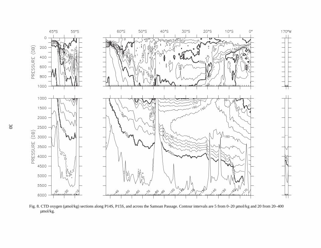
Fig. 8. CTD oxygen (µmol/kg) sections along P14S, P15S, and across the Samoan Passage. Contour intervals are 5 from 0–20 µmol/kg and 20 from 20–400µmol/kg.

30

31

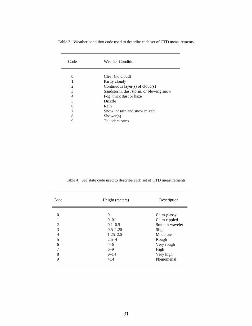
Table 3. Weather condition code used to describe each set of CTD measurements.

Code Weather Condition

0 Clear (no cloud)1 Partly cloudy2 Continuous layer(s) of cloud(s)3 Sandstorm, dust storm, or blowing snow4 Fog, thick dust or haze5 Drizzle6 Rain7 Snow, or rain and snow mixed8 Shower(s)9 Thunderstorms

Table 4. Sea state code used to describe each set of CTD measurements.

Code Height (meters) Description

0 0 Calm-glassy1 0–0.1 Calm-rippled2 0.1–0.5 Smooth-wavelet3 0.5–1.25 Slight4 1.25–2.5 Moderate5 2.5–4 Rough6 4–6 Very rough7 6–9 High8 9–14 Very high9 >14 Phenomenal

32

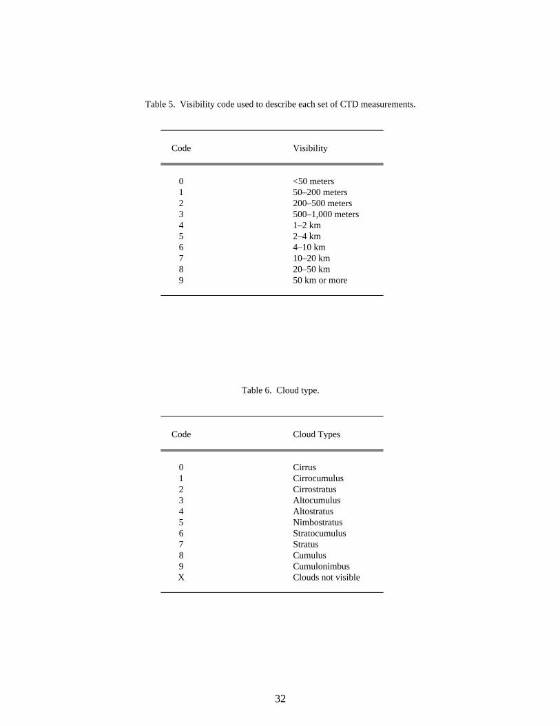
Table 5. Visibility code used to describe each set of CTD measurements.

Code Visibility

0 <50 meters1 50–200 meters2 200–500 meters3 500–1,000 meters4 1–2 km5 2–4 km6 4–10 km7 10–20 km8 20–50 km9 50 km or more

Table 6. Cloud type.

Code Cloud Types

0 Cirrus1 Cirrocumulus2 Cirrostratus3 Altocumulus4 Altostratus5 Nimbostratus6 Stratocumulus7 Stratus8 Cumulus9 CumulonimbusX Clouds not visible

33

Table 7. Cloud amount.

Code Cloud Amount

0 01 1/10 or less but not zero2 2/10–3/103 4/104 5/105 6/106 7/10–8/107 9/108 10/109 Sky obscured or not determined

All CTD and Hydrographic Data can be obtained bycontacting K.E. McTaggart at [email protected].

Documents

NOAA DATA REPORT ERL PMEL-63 CTD/O MEASUREMENTS …