Embed Size (px)
Citation preview
Noise and vibration reduction for a mass-spring-dampersystemNoijen, R.P.F.
Published: 01/01/2002
Document VersionPublisher’s PDF, also known as Version of Record (includes final page, issue and volume numbers)
Please check the document version of this publication:
• A submitted manuscript is the author's version of the article upon submission and before peer-review. There can be important differencesbetween the submitted version and the official published version of record. People interested in the research are advised to contact theauthor for the final version of the publication, or visit the DOI to the publisher's website.• The final author version and the galley proof are versions of the publication after peer review.• The final published version features the final layout of the paper including the volume, issue and page numbers.
Link to publication
Citation for published version (APA):Noijen, R. P. F. (2002). Noise and vibration reduction for a mass-spring-damper system. (DCT rapporten; Vol.2002.063). Eindhoven: Technische Universiteit Eindhoven.
General rightsCopyright and moral rights for the publications made accessible in the public portal are retained by the authors and/or other copyright ownersand it is a condition of accessing publications that users recognise and abide by the legal requirements associated with these rights.
• Users may download and print one copy of any publication from the public portal for the purpose of private study or research. • You may not further distribute the material or use it for any profit-making activity or commercial gain • You may freely distribute the URL identifying the publication in the public portal ?
Take down policyIf you believe that this document breaches copyright please contact us providing details, and we will remove access to the work immediatelyand investigate your claim.
Download date: 30. May. 2018
CENTRO DE INVESTIGACION Y DE
ESTUDIOS AVANZADOS DEL 1.P.N
EINDHOVEN UNIVERSITY n ~ ~ N T T TAT O r I L L H ~ WLOGY
Noise and vibration reduction for a mass- spring-damper system
Ralf Noijen 444552 DCT 2002.63
Coaches
Dr. G. Silva Navarro Prof. Dr. H. Nijmeijer.
Eindhoven, November 2002.
Abstract In this work four control strategies are implemented in a mass-spring-damper system
in order to suppress undesired vibrations. The first is a passive control strategy while the other three are active control strategies. Two of them are classical, namely the Linear Quadratic Regulator (LQR) and PI-control. Generalized PI is the fourth strategy and can be qualified as a modern control strategy. The performances of the controllers are compared both experimentally and in simulations.
Contents
1 Introduction
2 Passive control . . . . . . . . . . . . . . . . . . . . . . . . 2.1 The system without absorber
. . . . . . . . . . . . . . . . . . . 2.2 Passive control with vibration absorber . . . . . . . . . . . . . . . . . . . . . . . . 2.3 Simulations for passive control
3 Linear Quadratic Regulator . . . . . . . . . . . . . . . . . . . . . . . . . . . . . . . . 3.1 Pole assignment
. . . . . . . . . . . . . . . . . . . . . . . . . 3.2 Linear Quadratic Regulator . . . . . . . . . . . . . . . . . . . . . . . . . . . . . 3.3 Simulations for LQR
4 PI control . . . . . . . . . . . . . . . . 4.1 Determining the gains of the PI control
. . . . . . . . . . . . . . . . . . . . . . . 4.2 Simulations for PI control
5 Generalized PI control . . . . . . . . . . . . . . . . . . . . . . . . . . . . . . . . 5.1 Flat output
. . . . . . . . . . . . . . . . . . . . . . . . . . . . 5.2 Controller design
. . . . . . . . . . . . . . . . . . . . . . . . . . 5.2.1 Proposed controller . . . . . . . . . . . . . . . . . . . . . . . 5.2.2 Tuning of the controller
. . . . . . . . . . . . . . . . . . . . . . . . . 5.3 Simulations for GPI control
6 Experiments . . . . . . . . . . . . . . . . . . . . . . . . . . 6.1 The experimental platform
. . . . . . . . . . . . . . . . . . . . . . . 6.2 Experiments for passive control 6.2.1 Experiment to obtain the anti-resonance frequency . . . . . . . .
. . . . . . . . . . . . . . . . . . . . 6.2.2 Experiment for passive control . . . . . . . . . . . . . . . . . . . . . . . 6.3 Experiments with active control
. . . . . . . . . . . . . . . . . . . 6.3.1 Experiments with LQR control . . . . . . . . . . . . . . . . . . . . . . 6.3.2 Experiments for PI control
CONTENTS
6.3.3 Experiments for Generalized PI control . . . . . . . . . . . . . . . 33 6.3.4 Comparison of the experimental results . . . . . . . . . . . . . . . 34
7 Conclusions and recommendations 35
A M-files: PIfindgain 37
B Simulink model: Passive control
C Simulink model: LQR control
D Simulink models: PI control 43
E Simulink model: @PI control 45
F ECP programs: LQR
G ECP programs: PI
H ECP programs: Generalized PI
I T-c IULGI -mn+- l l l a u ; ~ ~ on CINVESTN=IPhT
Chapter 1
Introduction
Vibration control is a valuable tool in attenuating undesired vibrations in mechanical systems. Vibration control can be categorized in three main concepts: passive, semi- active and active vibration control.
Passive control requires no control input. When the parameters and the dynamics of a system are known and when a perturbation exists of a known frequency then passive control can be a very useful tool. The main idea is to change the frequency response of the system by adding stilrness and dampifig to the system. When dampifig and stiffness are added depending on the operating conditions one can speak about semi- active control. Physically it is difficult to add stiffness to a system, so in practice springs with adjustable spring characteristics are used.
In the past many active control strategies are developed. Active control can be divided in two groups, namely classical and modern control. A Linear Quadratic Regu- lator is a classical active control strategy. The working principle of the Linear Quadratic Regulator is to change the pole locations of the system by using state feedback. The difference with ordinary state feedback control is that the gains of the controller are determined by minimizing a cost function. This cost function depends on the control effort and the performance of the controller. In many mechanical systems it is not pos- sible to determine all the states of the system that are needed in the LQR control. PI control only needs an output and the same output that is integrated. The gains for the controller can not be determined, but an indication of the magnitude of the gains can be obtziried by the method of Zieg!€r-Nicho!s.
An example of a modern strategy that has recently been developed is generalized PI control. M e n a control system is differential flat it is possible to reconstruct the states of the system by integrals of the output and the input and also guarantees controllability. This property simplifies the analysis and design of the Generalized PI controller that is able to achieve asymptotic output tracking.
A mass-spring-damper system that consists of mass carriages that are connected with springs is used as a carrier to compare the control strategies that are mentioned before. The comparison is done regarding robustness and performance both experimentally and in simulations.

CHAPTER 1. INTRODUCTION
This report is organised as follows. In the first chapter passive control is explained in theory and implemented in simulations. The vibration absorber that is used for the passive control is maintained for the other controllers which makes the system underac- tuated. In chapters 3,4 and 5 are respectively the classical LQR and PI controller and the modern Generalised PI controller explained and simulated. In chapter 6 are some experiments made. The report is closed with a conclusion and some recommendations.
Chapter 2
Passive control
The vibration absorber that is discussed in this chapter is a useful tool to control vibra- tions with a single known frequency without any control effort. First the system without an absorber is discussed before the system with the vibration absorber is discussed.
2.1 The system without absorber
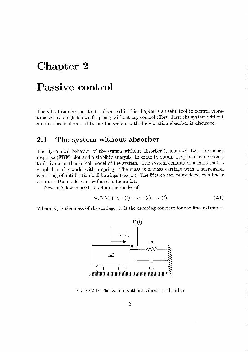
The dynamicai behavior of the system without absorber is analyzed by a frequency response (FRF) plot and a stability analysis. In order to obtain the plot it is necessary to derive a mathematical model of the system. The system consists of a mass that is coupled to the world with a spring. The mass is a mass carriage with a suspension consisting of anti-friction ball bearings (see [I]). The friction can be modeled by a linear damper. The model can be found in figure 2.1.
Newton's law is used to obtain the model of:
Where m2 is the mass of the carriage, c2 is the damping constant for the linear damper,
Figure 2.1: The system without vibration absorber
3
CHAPTER 2. PASSIVE CONTROL
Figure 2.2: FRF of system (2.1) without absorber
k2 is the linear spring coefficient and 2 2 the position of the mass with 22 and Z2 its velocity and acceleration. F( t ) represents the perturbation. In order to obtain a FW a Laplace transformation is performed on (2.1). This results in the following transfer function:
X2(4 - G(s) = - - 1
F (s) (m2s2 + c2s + k2) (2.2)
The parameters are taken from the experimental setup as:
m2 = 2.839 kg, k2 = 340 N/m, c2 = 0.01 Ns/m (2.3)
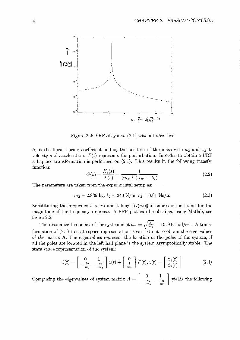
Substituting the frequency s = i w and taking [[G(iw)[lan expression is found for the magnitude of the frequency response. A FRF plot can be obtained using Matlab, see figure 2.2.
The resonance frequency of the system is at w, = 2 = 10.944 rad/sec. A trans- r formation of (2.1) to state space representation is carried out to obtain the eigenvalues of the matrix A. The eigenvalues represent the location of the poles of the system, if all the poles are located in the left half plane is the system asymptotically stable. The state space representation of the system:
Computing the eigenvalues of system matrix A = 1 c2 ] yields the following
m2
2.2. PASSIVE CONTROL WITH VIBRATION ABSORBER
Figure 2.3: The system with absorber
pole locations: pl,, = -1.761 2 x & 10.943i
The real parts of the eigenvalues are small but negative which means that the system is asymptotically stable. The imaginary part can be recognized as the resonance frequency of the system.
2.2 Passive control with vibration absorber
The system with vibration absorber consists of a primary mass ma and an absorber ml (see figure 2.3). U ( t ) = 0 because the control is passive. The main idea of passive control is that the response on vibrations for the primary system is minimized when the excitation frequency coincides with the uncoupled natural undamped eigenfrequency of the absorber.
In order to obtain a FRF plot it is necessary to describe the system mathematically. Newton's law yields:
m l x l ( t ) + c l x l ( t ) + k l x l ( t ) - klx2(t) = U ( t ) (2.5)
m2x2(t) + c2i3 ( t) + k2x2(t) + kl ( 2 2 ( t ) - xl ( t ) ) = F ( t )
By taking the Laplace transform of (2.5), with Il' = 0, the transfer hnction G ( s ) , h t gives a relationship between the amplitude of movement of the primary system and the excitation, is given by:
Substituting s = iw and taking IIG(iw) 1 1 gives an expression for the magnitude of the FRF of the primary system. The parameters are taken from the experimental setup as:
ml = 1.586 kg, kl = 745 N/m, cl = 0.01 Ns/m (2-7)
6 CHAPTER 2. PASSIVE CONTROL
The other parameters are the same as in the system without absorber. The FRF of the passive control can be compared with the FRF of the system without absorber in figure
Figure 2.4: The FRF of system (2.7) (solid) and of system (2.1) (dashed)
For the system with absorber two resonance frequencies can be recognized namely close to the natural eigenfrequencies of the system because the damping is very small (see [2]). From the figure it can be seen that the eigenfrequencies are near 9 and 28 Hertz and the anti-frequency is near 22 Hertz. The anti-resonance frequency should be near
the uncoupled natural eigenfrequency of the absorber, wnl = 6 = 21.673 radlsec.
The eigenfrequencies can be determined by the pole locations. Equation (2.5) can be transformed to a set of first order differential equations by introducing the state vector
T x2 5 2 ] -
The eigenvalues of matrix A give the following pole locations:
2.3. SIMULATIONS FOR PASSIVE CONTROL 7
The eigenfrequencies of the system are indeed near 9 and 28 Hertz according to the pole locations, namely 27.934 and 8.4938 Hertz. The location of the poles indicate that the system is asymptotically stable.
The advantage of the passive control is clear: it is possible to tune the absorber in a way that the gain at the excitation frequency is very low. This is achieved with no control effort. Figure 2.4 shows two resonance peaks. This implies that in the presence of some noise in the excitation the primary system will excite with higher amplitudes.
2.3 Simulations for passive control
In order to show the conclusions of the previous section some simulations are carried out with Matlab's Simulink. In passive control are initial conditions very important to tune the absorber. The simulations are carried out with the initial conditions that are calculated below.
To obtain good results in simulation the initial conditions are very important. How- ever in experiments this is not the case because friction is not taken into account in the model. For the system of (2.5) the next solution (and its derivatives) is proposed:
xl (t) = A cos(wt) , 21 (t) = -Aw sin(wt) , xl (t) = -Aw2 cos(wt) (2.10)
x2(i) = 3 C O S ( W ~ ) , k2(t) = - 3 w sin(wt), Z2(t) = - B W ~ C O S ( W ~ )
Substituting this and w = 6 (because this is the excitation frequency that the ab-
sorber is tuned to) in (2.5) at t = 0 (where sin(wt) = 0, cos(wt) = 1 and F( t ) =
Fo cos(wt) = Fo) yields:
The first equation gives B = 0, which is desirable because the amplitude of the movement of the primary system should be 0. Substituting B = 0 in the second equation yields.
The initial conditions used in the simulations are xl(0) = A, ~ ~ ( 0 ) = x2(0) = 540) = 0. The Simuiink schemes can be found in appendix B. The excitation is F = 3 cos(2i.673). Simulations without the addition of noise are carried out on both the system without (2.1) and with (2.3) absorber. From these simulations it can be concluded that; the absorber is a very useful tool since the amplitude of the vibration for the system without absorber is 5 . m and for the system with absorber 3 . lop6 m. The amplitude of the vibration for the system with absorber when white gaussian noise with mean zero and variance 0.02 is added is 1 . m. This indicates that the passive control is not robust to noise but still shows better results than the system without absorber. In figure 2.5 the result of a simulation for the passive controller without the addition of noise can be found.
CHAPTER 2. PASSIVE CONTROL
Figure 2.5: Response of primary system, see figure (2.3), without the addition of noise

Chapter 3
Linear Quadratic Regulator
The first control strategy used to control the primary system by actuating the absorber is the Linear Quadratic Regulator (LQR). LQR is an optimized state feedback control strategy. First state feedback control is explained using pole placement. Then LQR is used to find suitable pole locations and the corresponding gains.
3.1 Pole assignment
In order to place the poles of the system in arbitrary positions the system should be observable and controllable. The system to be controlled is represented by figure 2.3 and the mathematical model of (2.8). It has already been proven that the system is stable. To prove observability the observability matrix [ C CA CA2 CA3 ] should be of full rank (4) . To prove controllability the controllability matrix: [ B AB A 2 ~ A3B ] should be of full rank. Here the system is given by (2.8) with the output:
y ( t ) = C z (t) + D U ( t )
y ( t ) = [ o 0 1 O ] z ( t )
Resulting in the observability matrix and its rank:
I 0 0 1 0
obs = 0 0 0 1
262.42 0 -382.18 -3.5224 x 1 r a n k = 4 (3.2)
-. 924 33 262.42 1.346 2 -382.18
And the controllability matrix and its rank:
10 CHAPTER 3. LINEAR QUADRATIC REGULATOR
Thus it can be concluded that the system is stable, observable and controllable. This implies that the poles can be placed at arbitrary positions using state feedback control. The control law used for state feedback control is:
The result of substituting K = [ Kl K2 K3 K4 ] in (2.8) yields:
The characteristic polynomial can be derived from system matrix A:
The gains of the system can be found by substituting the desired pole locations in the characteristic polynomial.
3.2 Linear Quadratic Regulator The LQR determines the gains by minimizing a cost function. First the minimization procedure will be highlighted. Then the LQR is applied to the system, a FRF plot is made and discussed and simulations are carried out.
The cost function that is to be minimized is a quadratic time domain performance index:
it is proven (see [GI) that (3.6) is minimized by choosing the feedback gain K to be:
Where S = ST > 0 is the solution of the Riccati equation:
A and B are the system matrices as determined in (3.5) and Q and R are the user defined weighting matrices of the cost function. The performance of the controller will depend on the values for the weighting matrices. The Q matrix puts more emphasis on
3.2. LINEAR QUADRATIC REGULATOR
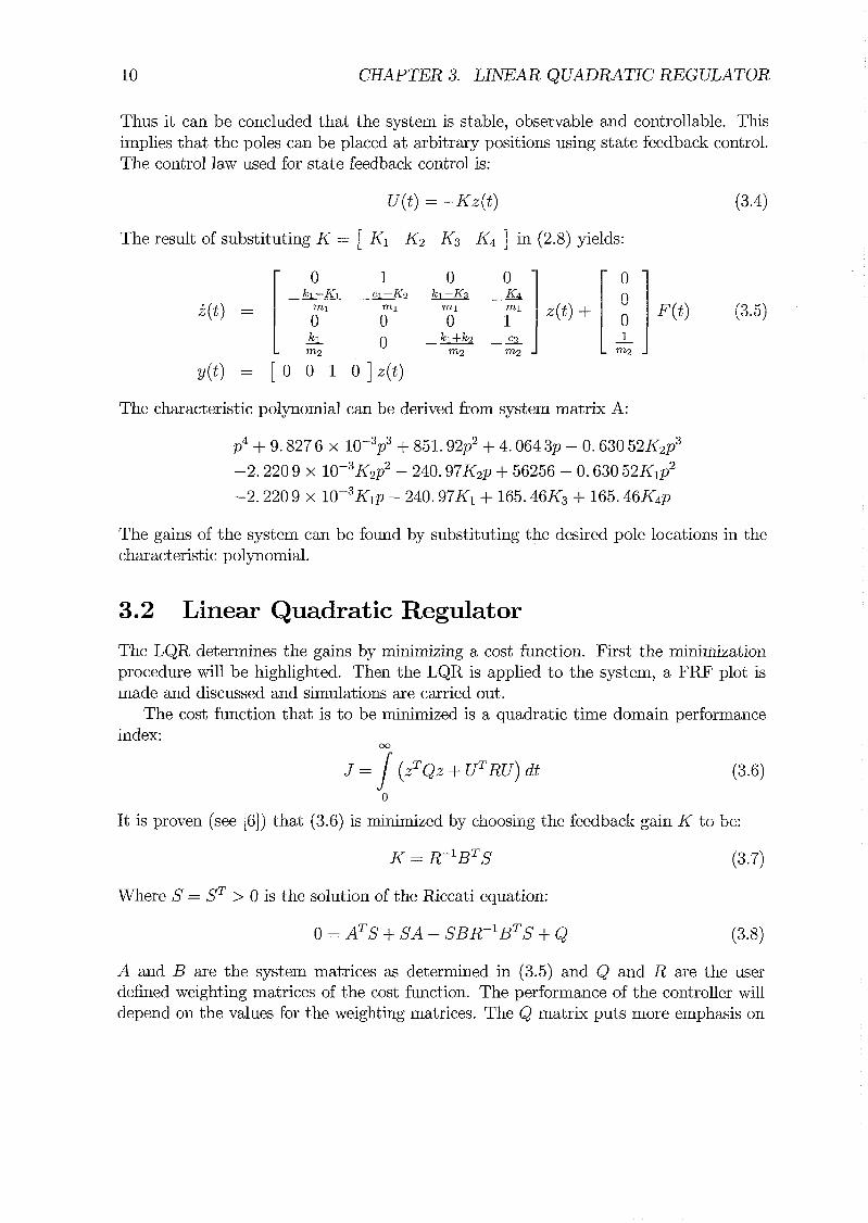
Figure 3.1: Bode plots for system with absorber (dash-dot) , without absorber(so1id) and LQR (dashed)
the performance of the controller and the R matrix puts more emphasis on the control effort. The objective is to control the position of the primary system without a big control effort. It appeared that the following weighting matrices suffice this demand:
To determine the gain the Matlab command 1qr.m is used. This results in the feedback gain:
The resulting pole locations p = / -1'2896 28'08512 1 . This implies that the eigenfre- -4.0243 f 9.0000~
L 1
quencies will be wnl = 9 rad/sec. and w,z = 28.0851 rad/sec. A frequency response plot or Bode plot can easily be obtained by using the b0de.m command in Matlab, see figure 3.1.From figure 3.1 can be concluded that the control is more robust to noise because the resonance peaks are lower but the feature of the vibration absorber in the passive control in terms of the anti resonance is not preserved. Simulations are made to justify this conclusion.
12 CHAPTER 3. LINEAR QUADRATIC REGULATOR
3.3 Simulations for LQR It is necessary that the primary system can be controlled to a reference position. For this case an additional control effort has to be made. This additional control effort can be determined by considering the system in state space notation:
The control force will be defined as:
Where y, is the reference point and G the additional gain to bring the system in the desired equilibrium position. Plugging the control force into the system yields:
In the equilibrium i ( t ) is zero. This yields the equilibrium:
The output at the equilibrium is defined as:
So y = y, yields for G: G=- 1
C(A - BK)-lB
It should be noted that this addition in the control effort will make the performance index (3.6) to go to infinity.
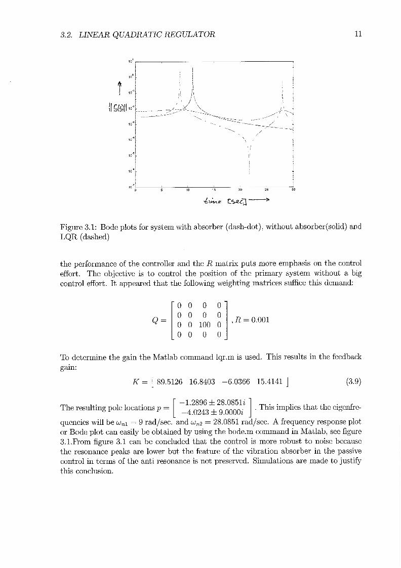
Now simulations can be made with a reference point. The used Sirnulink models can be found in appendix B. Simulations are carried out with and without noise. From the simulations it could be concluded that the amplitude of the vibration is almost the same in the noisy case and in the simulations without noise. This amplitude is about 1000 times higher than in the simulations for passive control. This justifies that the afiti-resonance as we!! &s the resoiiamzs diszppemed. Another disadvantage of the LQIt control is that the complete state has to be known. Fast asymptotic tracking is achieved with a small control input (about 6 Newton) with this controller. In figure 3.2 can the result of the simulation with the addition of noise be found. The noise and perturbation are the same as in the simulations for passive control.
It is necessary to find a control strategy that conserves the anti resonance and pro- vides robustness to noise. In the next chapter another classical control strategy will be applied to the system, namely PI control. Using this control strategy only the position of the primary system has to be known to control the system.
3.3. SIMULATIONS FOR LQR
Figure 3.2: Response of primary system with LQR control in presence of noise

Chapter 4
The second classical control theory to be implemented is a PI controller. First the controller is proposed. The magnitude of the gains follow from a method using root-locus and Ziegler-Nichols (see 141). A frequency response plot is made and finally simulations are made.
The standard form of the PI controller is: t
1 U(t) = K (e,(t) + - 1 e, (t) dt)
T, J 0
Where e,(t) = y,(t) - y(t) and K and T, are the gains. To obtain an idea of the magnitude of the gains the Ziegler-Nichols method is used.
4.1 Determining the gains of the PI control
To use the Ziegler-Nichols method it is necessary to determine the critical times and the critical gain. The critical times can be derived from the resonance frequencies of the svstem:
The critical gain of the system is that gain (in U(t) = Ky) that makes the system instabie. To determine this gain the riocus.m program in Matiab is used. As an input again the system matrices of (2.8) are used as well as a prescribed vector of gains. The critical gains c2n be seen as the lower and upper bounds of the gains for which the system is stable:
Kcl = -340, Kc2 = 755 (4.3) The Ziegler-Nichols frequency response method (see [4]) gives the next indication of the gains of the system:
16 CHAPTER 4. PI CONTROL
The system is very close to instability due to low damping. That makes it more difficult to find gains that keep the system stable. To find gains P1findgain.m (see appendix A) in Matlab is used. The algorithm computes the pole locations for the closed loop system for different gains. The state space representation for the closed loop system can be ob-
t T
tained by adding a state to the system: ( t ) = [ x1 (t) il (t) x2 (t) 22 (t) J x2 (t) ] . 0
The open loop system in state space representation is given in equation (2.8). With t
the additional state and U(t) = K(-x2(t) + $ J(-xz (t)) the closed loop state space D
represent ation is:
The pole locations are determined by computing the eigenvalues of the matrix A. This process is repeated for different gains. One example of gaim that result in a stable closed loop system is : K = 0.2 and T, = 0.18001. This results in the following pole locations:
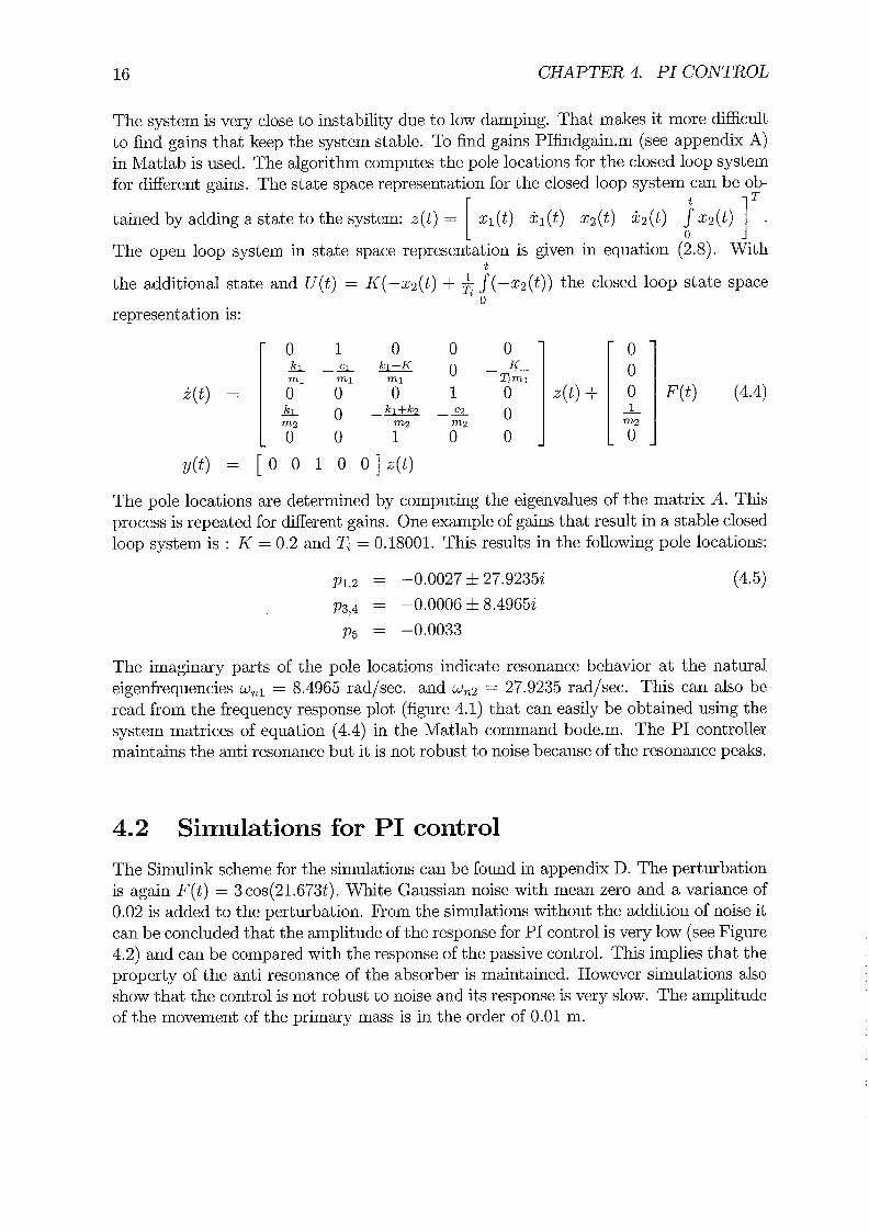
The imaginary parts of the pole locations indicate resonance behavior at the natural eigenfrequencies wnl = 8.4965 rad/sec. and wn2 = 27.9235 rad/sec. This can also be read from the frequency response plot (figure 4.1) that can easily be obtained using the system matrices of equation (4.4) in the Matlab command b0de.m. The PI controller maintains the anti resonance but it is not robust to noise because of the resonance peaks.
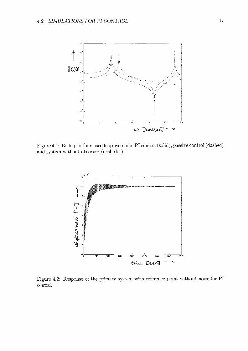
The Simulink scheme for the simulations can be found in appendix D. The perturbation is again F ( t ) = 3 cos(21.673t). White Gaussian noise with mean zero and a variance of 0.02 is added to the perturbation. From the simulations without the addition of noise it can be concluded that the amplitude of the response for PI control is very low (see Figure 4.2) and can be compared with the response of the passive control. This implies that the property of the anti resonance of the absorber is maintained. However simulations also show that the control is not robust to noise and its response is very slow. The amplitude of the movement of the primary mass is in the order of 0.01 m.
4.2. SIMULATIONS FOR PI CONTROL
Figure 4.1: Bode plot for closed loop system in PI control (solid), passive control (dashed) and system without absorber (dash dot)
Figure 4.2: Response of the primary system with reference point without noise for PI control
Chapter 5
Generalized PI control
After the classical control techniques LQR and PI control a modern control technique is to be implemented to the system to conserve the anti-resonance and to get a more robust controller. It is usual that not all states of a system are measurable. It is usual to estimate the states by either using an asymptotic observer or online calculations of time derivatives of the available output systems. The idea of the Generalized PI controller is to construct an integrated state feedback controller based on structural estimates of the states of the system. The errors that occur ill that way can be compensated by integral actions. The flat output will first be derived because the controller is derived from this output. Also the reconstruction of the states is derived from the flat output. When all this is done the appropriate gains for the controller are derived using pole placement. The resulting bode plot will be derived and discussed. Finally simulations are carried out for the GPI controller.
5.1 Flat output
The system (2.8) has a flat output y = 2 2 . This means that the state variables and the input can be parameterized in terms of the output and a finite number of its time derivatives (see [12], [13] and [l4]). From now on a( t ) will be written as a to keep the expressions shorter. The parametrization is obtained from (2.8):
CHAPTER 5. GENERALIZED PI CONTROL
Here the constants are given by:
In the parametrization of the state variables and the input are derivatives of the out- put and inputs present. Also in the control law these derivatives are present. This is undesirable. A reconstruction of these derivatives is possible through integration of the
t last expression in (5.1). In order to keep the expressions shorter J Bdt will be written as
0 t 7
J , J J y d ~ d t as y etc. This procedure yields a parametrization of the derivatives 0 0
of the output in terms of the inputs, integrals of the inputs, the output and integrals of the output:
With the structural estimates:
Here U1, U2 and U3 are structural estimates for 0, i j and ~ ( ~ 1 . The error made in these structural estimates are depending on the perturbation and the initial conditions. Now the estimates are known, a controller can be proposed that is independent of derivatives of the output.

5.2. CONTROLLER DESIGN
5.2.1 Proposed controller
The proposed controller is:
The controller consists of three parts. The first part are the structural estimates (ay + a l e l + a2e2 + a3e3) that are supposed to cancel the dynarnical properties of part of the last expression of (5.1), that is (-ay - aly - a2y - a3y3) . However in the struc- tural estimates an error is made that is caused by the initial conditions and by the perturbation. The nature of the error caused by the initial conditions can be found in (5.7). These errors are of the type constant, linear (t) and parabolic (t2). Applying a Laplace transformation to these errors gives for the constant: $, for the ramp: 2 and for the parabolic function: $. Here integrators can easily be recognized. In order to compensate these errors three integrators are added to (5.9). The third part of the ce~tro! is an additional part of the dynamics that will caduse the closed loop dynamics to be asymptotically stable, that is (-K4y - K3e1 - K202 - K1e3). When the inte- grators compensate the errors made in the structural estimates then the characteristic polynomial of the closed loop system is of the Hurwitz type which means that the poles are all located in the open left complex half plane.
5.2.2 Tuning of the controller
Choosing appropriate values for the gains Kl , K2, K3, K4, K5, K6 and K7, is done by pole placement. For this purpose the characteristic equation of the closed loop system has to be found. The characteristic equation is the denominator of the transfer function G(s) = &. For this purpose a Laplace transformation is performed on (2.5) :
F ( s )
To obtain the transfer function % (5.8) is substituted in (5.9) and this result is sub- stituted in (5.10) after a Laplace transformation. The values for the masses, spring constants and damping constants are the same as in the previous chapters. The denom-
22 CHAPTER 5. GENERALIZED PI CONTROL
inat or, or characteristic equation, contains the following components:
1.0s7 + (4.672 9 x lop8 + 1.0K1) s6 (5.11)
(-4.576 9 x ~ O - ~ K ~ + 1.413 7 x + 1 . 0 ~ 2 ) s5
(5.457 3 x - 3.630 5 x - 4.576 9 x I O - ~ K ~ + 1 . 0 ~ 3 ) s4
(5.162 4 x ~ o - ~ K ~ + 1.610 2 x 1ov7K3 + 2.457 + l .0K4 - 7.853 2 x I O - ~ K ~ ) s3
(-35. 781K1 - 6.465 6 x + 5.165 9 x 1oy2K3 + l.0K5 + 0.723 72) s2
(-2966.2 - 0.151 02K1 + 4.275 3 x 1 0 - ~ ~ 3 - 1.6262 x 10-~K2 + 1 . 0 ~ 6 ) s
-1943. 3K1 - 7.25i 4 x 1 0 - 2 ~ 2 + 1.0K7 + 63.297
The desired dynarnical behavior is:
(s2 + 2[w,s + w:)~ (S + b)
A common choice in engineering practice for the damping constant is J = 0.52/2. The chosen value for both the natural eigenfrequency w, and the additional pole b is 20. The resulting characteristic polynomial is:
l.0s7 + 104. 85s6 + 5297. l s5 + 1.625 1 x 10⁵s4 + 3.250 2 x 10⁶s3 + 4.237 6 x 10⁷s2 + 3.355 3 x 10⁸s + 1.28 x lo9
The gains are then found as:
K1 = 104.85, K2 = 5297.1, K3 = 1.625 1 x lo5, K4 = 3.249 9 x lo6 (5.13)
K5 = 4 . 2 3 7 1 ~ 1 0 ~ , ~ ~ = 3 . 3 5 5 3 ~ 1 0 ~ , ~ ~ = 1 . 2 8 0 2 ~ 1 0 ~
The nominator of the resulting transfer function G(s) = $$ is:
And the denominator:
1.0s7 + 104. 85s6 + 5296. 9s5 + 1.625 1 x 10⁵s4 + (5.15)
3.250 3 x lo6s3 + 4.2378 x 10⁷s2 + 3.355 4 x 10⁸s + 1.280 1 x 10'
Due to numerical problems is the denominator of the resulting transfer function a little bit different from the desired characteristic polynomial. The biggest difference in the coefficients is of the order 0.02 percent. This has a big influence on the pole locations:
sl = -20.002, s2,3 = -15.006 f 13.631i (5.16)
-14.113 f 15.1532, S6,7 = -13.305 5 13.644.2 S4,5 -
The desired pole locations are:
S l = -20, S2,3,4,5,6,7 = -14.142 f 14.1422
The frequency response plot can be found in figure 5.1. The bode plot for the GPI control indicates that this control is able to meet the objectives of the project. It preserves the anti-resonance that is characteristic for the vibration absorber and is robust to noise. To justify these conclusions simulations are carried out for noisy and non-noisy cases with a reference trajectory.

5.3. SIMULATIONS FOR GPI CONTROL
Figure 5.1: Bode plot for GPI control (solid), for no absorber (dash-dot) and for passive control (dashed)
5.3 Simulations for GPI control Simulations are carried out with a perturbation of F = 3cos(21.763t). In order to see whether the controller achieves fast asymptotic tracking is a reference signal created that the primary system should track. The structural estimates give estimates for the output and three time derivatives of the output. Therefore should the reference signal be smooth up until the fourth time derivative of the reference signal. Then the control effort is reduced. The reference is a zero signal up to 4.5 seconds.. Then a smooth function is employed to bring the reference from zero to one em. After this a reference of 1 cm is maintained.
The simulation starts at t = -4.5 seconds, which means that the reference trajectory starts at to = 0 and ends at tf = 1 second. The demands for the reference signal r are:
Where r o = 0 and rf = 0.01 m. With these demands for the function that describes the reference trajectory all reference states used by the controller are differentially continu- ous. Because there are ten demands a function with ten variables has to be proposed to solve the problem. The proposed function for the trajectory is:
Differentiating t h s signal four times yields a system of 10 equations because there are conditions at to and t f . Solving this system results in the following coefficients for the
24 CHAPTER 5. GENERALIZED PI CONTROL
reference signal:
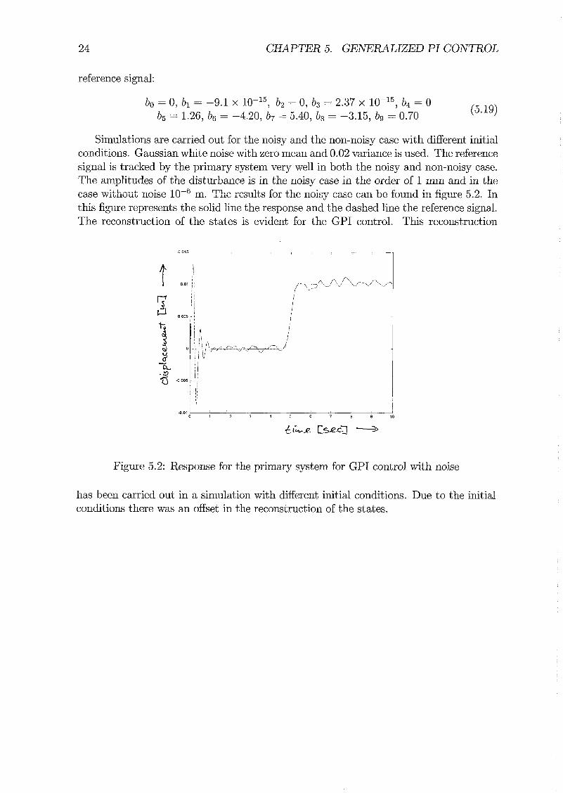
Simulations are carried out for the noisy and the non-noisy case with different initial conditions. Gaussian white noise with zero mean and 0.02 variance is used. The reference signal is tracked by the primary system very well in both the noisy and non-noisy case. The amplitudes of the disturbance is in the noisy case in the order of 1 mm and in the cme w;tho-Gt noise 19-6 'PLA - ..It L r tho -A '
lllG ~es,,s lul ..., ..,lsy case ~2x1 be feund in figlxe 5.2. In this figure represents the solid line the response and the dashed line the reference signal. The reconstruction of the states is evident for the GPI control. This reconstruction
Figure 5.2: Response for the primary system for GPI control with noise
has been carried out in a simulation with different initial conditions. Due to the initial conditions there was an offset in the reconstruction of the states.
Chapter 6
Experiments
Before the experiments for the described control strategies are carried out a short de- scription of the experimental setup is given. After that experiments for the strategies are carried out.
6.1 The experimental platform
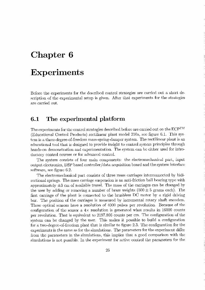
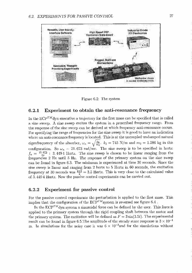
The experiments for the control strategies described before are carried out on the ECPTM (Educational Control Products) rectilinear plant model 210a, see figure 6.1. This sys- tem is a three-degree-of-freedom mass-spring-damper system. The rectilinear plant is an educational tool that is designed to provide insight to control system principles through hands-on demonstration and experimentation. The system can be either used for intro- ductory control courses or for advanced control.
The system consists of four main components: the electromechanical part, input output electronics, DSP based controller/dat a acquisition board and the system interface software, see figure 6.2.
The electromechanical part consists of three mass carriages interconnected by bidi- rectional springs. The mass carriage suspension is an anti-friction ball bearing type with approximately f 3 cm of available travel. The mass of the carriages can be changed by the user by adding or removing a number of brass weights (500 f 5 grams each). The first carriage of the plant is connected to the brushiess DC motor by a rigid driving bar. The position of the carriages is measured by incremental rotary shaft encoders. These optical sensors have a resolution of 4000 pulses per revolution. Because of the configuration of the sensor a 4x resolution is generated what results in 16000 counts per revolution. That is equivalent to 2197.866 counts per cm. The configuration of the system can be changed by the user. This makes it possible to build a configuration for a two-degree-of-freedom plant that is similar to figure 2.3. The configuration for the experiments is the same as for the simulations. The parameters for the experiment differ from the parameters in the simulations, this implies that a good comparison with the simulations is not possible. In the experiment for active control the parameters for the
CHAPTER 6. EXPERIMENTS
Figure 6.1: The rectilinear plant
masses are: ml = 1.839 kg, m2 = 3.05 kg
The friction is very small and can be assumed to be 0.01 N/s2. The parameters for the spring constants are obtained through experiments. To determine the spring constant of the first spring, k l , five times five experiments are carried out for forces ranging from 2 Newton until 10 Newton. In those experiments the elongation x of the springs is measured and the spring constant is obtained by the relation
The average of the 25 experiments is taken and the result is kl = 745 N/m. The same experiment for forces ranging from 1 to 5 Newton is carried out for the second spring and the result is k2 = 340 N/m.
6.2 Experiments for passive control
In order to do experiments for passive control the configuration is changed. The entire system is reversed because the brushless DC motor is used to apply the perturbation. First an experiment is carried out to find the anti-resonance frequency of the system. This frequency will be used in the experiment for the excitation frequency. In simulations noise is added however in experiments noise is present in the system. The characteriza- tion of the experimental noise is not done. This implies that the noise in the simulations is different from the noise that is experienced in the experiments.
6.2. EXPERIMENTS FOR PASSIVE CONTROL
Inn~vativc. thought. Provaklnq Experimenls
_ - . V w - ,
: k?- ~n second hrkchmism osc~llatoty shown mode
Figure 6.2: The system
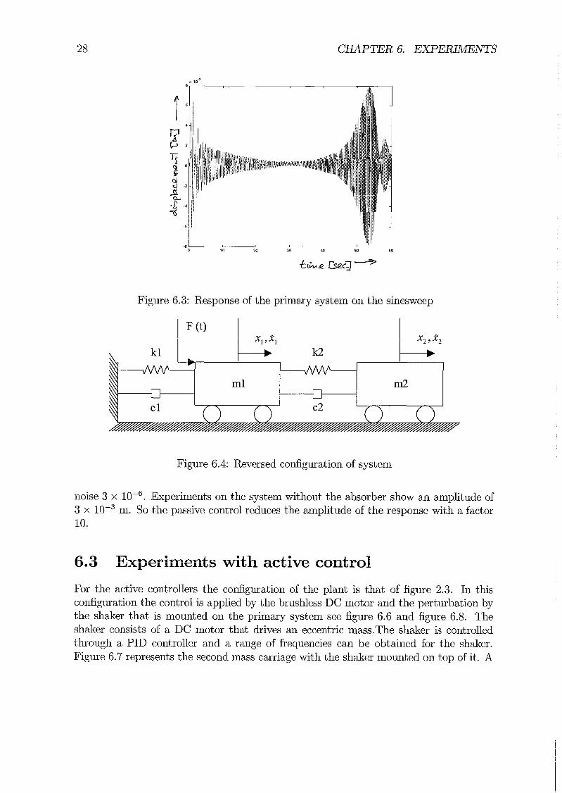
Experiment to obtain the anti-resonance frequency
In the ECPTMdyn executive a trajectory for the f i s t mass can be specified that is called a sine sweep. A sine sweep excites the system in a prescribed frequency range. From the response of the sine sweep can be derived at which frequency anti-resonance occurs. For specifying the range of frequencies for the sine sweep it is good to have an indication where an anti-resonance frequency is located. This is at the uncoupled undamped natural
eigenfrequency of the absorber, wn = p. m2 k2 = 745 N/m and m2 = 1.586 kg in this
configuration. So wn = 21.673 rad/sec. The sine sweep is to be specified in hertz: 21.673 : 3.4494 Hertz. The sine sweep is chosen to be linear ranging from the fn = -
2? frequencies 2 Hz until 5 Hz. The response of the primary system on the sine sweep can be found in figure 6.3. The minimum is experienced at time 30 seconds. Since the sine sweep is linear and ranging from 2 hertz to 5 Hertz in 60 seconds, the excitation frequency at 30 seconds was = 3.5 Hertz. This is very close to the calculated value of 3.449 4 Hertz. Now the passive control experiments can be carried out.
6.2.2 Experiment for passive control
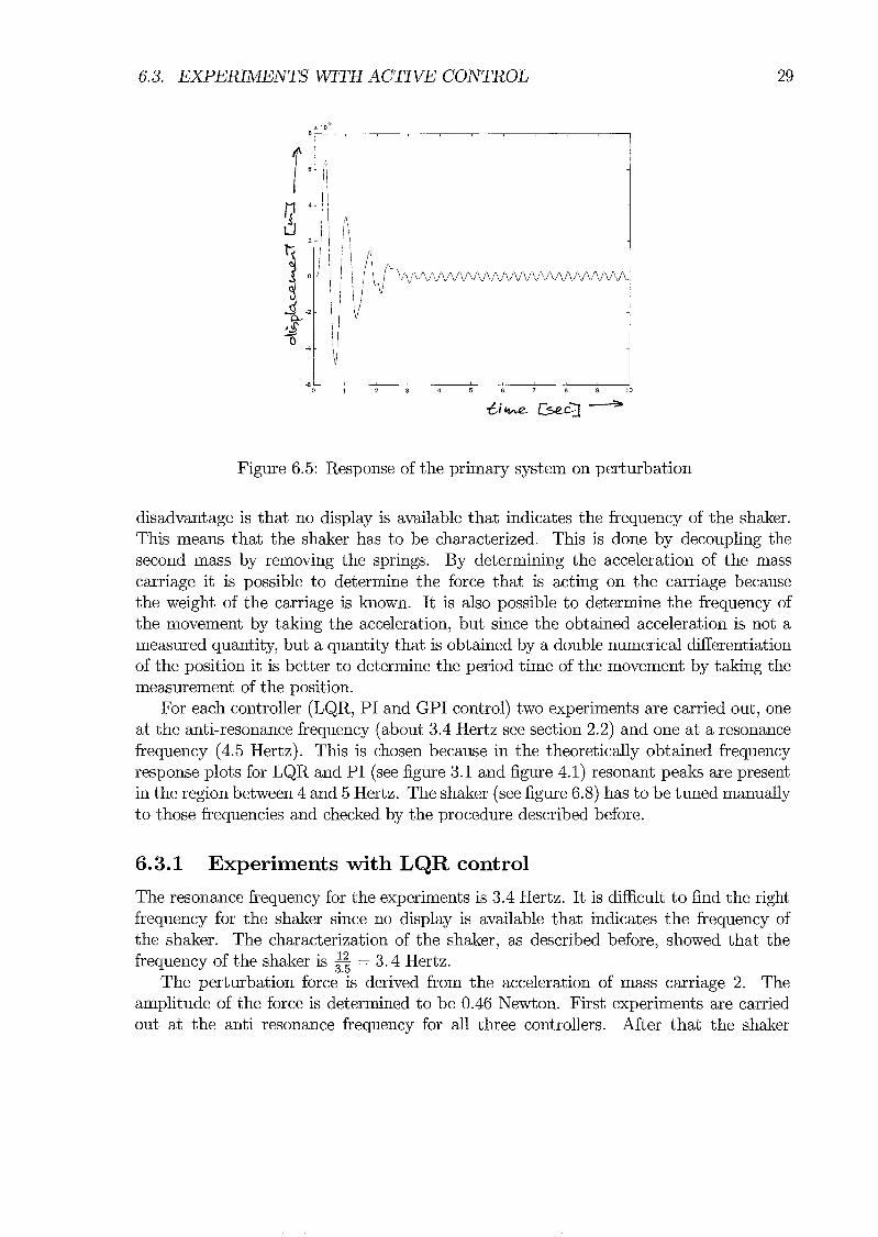
For the passive control experiments the perturbation is applied to the first mass. This implies that the configuration of the ECPTMsystem is reversed see figure 6.4 .
In the ECPTMdyn system a sinusoidal force can be defined by the user. This force is applied to the primary system through the rigid coupling shaft between the motor and the primary system. The excitation will be defined as F = 3 sin(3.5t). The experimental result can be found in figure 6.5.The amplitude of the steady state response is 3 x m. In simulations for the noisy case it was 6 x 10-~and for the simulations without
CHAPTER 6. EXPERIMENTS
Figure 6.3: Response of the primary system on the sinesweep
Figure 6.4: Reversed configuration of system
noise 3 x lop6. Experiments on the system without the absorber show an amplitude of 3 x m. So the passive control reduces the amplitude of the response with a factor 10.
6.3 Experiments with active control
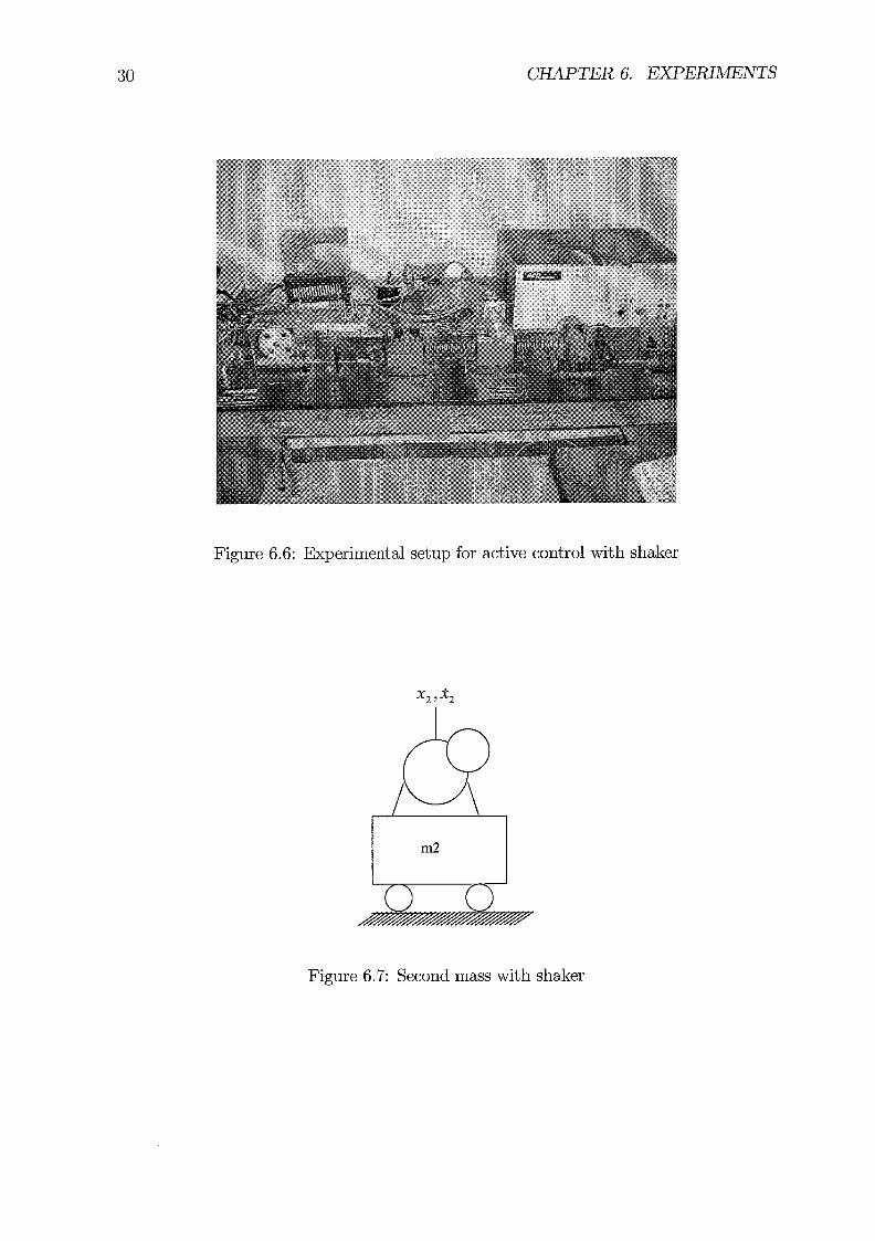
For the active controllers the configuration of the plant is that of figure 2.3. In this configuration the control is applied by the brushless DC motor and the perturbation by the shaker that is mounted on the primary system see figure 6.6 and figure 6.8. The shaker consists of a DC motor that drives an eccentric mass.The shaker is controlled through a PID controller and a range of frequencies can be obtained for the shaker. Figure 6.7 represents the second mass carriage with the shaker mounted on top of it. A
6.3. EXPERIMENTS WITH ACTIVE CONTROL
Figure 6.5: Response of the primary system on perturbation
disadvantage is that no display is available that indicates the frequency of the shaker. This means that the shaker has to be characterized. This is done by decoupling the second mass by removing the springs. By determining the acceleration of the mass carriage it is possible to determine the force that is acting on the carriage because the weight of the carriage is known. It is also possible to determine the frequency of the movement by taking the acceleration, but since the obtained acceleration is not a measured quantity, but a quantity that is obtained by a double numerical differentiation of the position it is better to determine the period time of the movement by taking the measurement of the position.
For each controller (LQR, PI and GPI control) two experiments are carried out, one at the anti-resonance frequency (about 3.4 Hertz see section 2.2) and one at a resonance frequency (4.5 Hertz). This is chosen because in the theoretically obtained frequency response plots for LQR and PI (see figure 3.1 and figure 4.1) resonant peaks are present in the region between 4 and 5 Hertz. The shaker (see figure 6.8) has to be tuned manually to those frequencies and checked by the procedure described before.
6.3.1 Experiments with LQR control
The resonance frequency for the experiments is 3.4 Hertz. It is difficult to find the right frequency for the shaker since no display is available that indicates the frequency of the shaker. The characterization of the shaker, as described before, showed that the frequency of the shaker is $ = 3.4 Hertz.
The perturbation force 1s derived from the acceleration of mass carriage 2. The amplitude of the force is determined to be 0.46 Newton. First experiments are carried out at the anti resonance frequency for all three controllers. After that the shaker
CHAPTER 6. EXPERIMENTS
Figure 6.6: Experimental setup for active control with shaker
Figure 6.7: Second mass with shaker
6.3. EXPERIMENTS WITH ACTIVE CONTROL
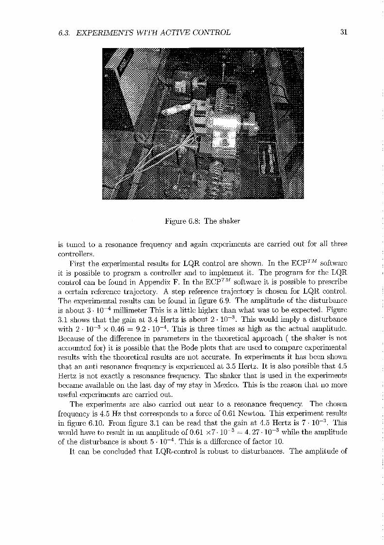
Figure 6.8: The shaker
is tuned to a resonance frequency and again experiments are carried out for all three controllers.
First the experimental results for LQR control are shown. In the ECPTM software it is possible to program a controller and to implement it. The program for the LQR control can be found in Appendix F. In the ECPTM software it is possible to prescribe a certain reference trajectory. A step reference trajectory is chosen for LQR control. The experimental results can be found in figure 6.9. The amplitude of the disturbance is about 3 . lop4 millimeter Tlvs is a little higher than what was to be expected. Figure 3.1 shows that the gain at 3.4 Hertz is about 2 This would imply a disturbance with 2 . lop3 x 0.46 = 9.2 - This is three times as high as the actual amplitude. Because of the difference in parameters in the theoretical approach ( the shaker is not accounted for) it is possible that the Bode plots that are used to compare experimental results with the theoretical results are not accurate. In experiments it has been shown that an anti resonance frequency is experienced at 3.5 Eertz. it is also possible that 4.5 Hertz is not exactly a resonance frequency. The shaker that is used in the experiments became available on the last day of my stay in Mexico. This is the reason that no more useful experiments are carried out.
The experiments are also carried out near to a resonance frequency. The chosen frequency is 4.5 Hz that corresponds to a force of 0.61 Newton. This experiment results in figure 6.10. From figure 3.1 can be read that the gain at 4.5 Hertz is 7 . This would have to result in an amplitude of 0.61 x 7. lop3 = 4.27. loF3 while the amplitude of the disturbance is about 5 - lop4. This is a difference of factor 10.
It can be concluded that LQR-control is robust to disturbances. The amplitude of

CHAPTER 6. EXPERIMENTS
Figlxe 6.9: Experimental results for LQR control
Figure 6.10: Experiment for LQR at 4.5 Hz
6.3. EXPERIMENTS WITH ACTIVE CONTROL 33
the disturbance seems large to be a result of a anti resonance. It can be concluded that the anti resonance of the passive control is not present in the closed loop of LQR control.
6.3.2 Experiments for PI control
In the simulations for PI control is shown that the system converges very slowly to a reference. In the E C P ~ " software it is not possible to perform a step reference for the time that is necessary for the PI controller to converge. Now only a constant reference signal of 1 cm is wed for the primary system. The algorithm that is used can be found in Appendix 6;. The ECPTM system is not capable of doing measurements that take a long time. During the experiment with an perturbation with a frequency of 3.4 Hertz ten measurements are made. For every measurement the time started at zero again. It is not illustrative to show the measurements. In all measurements the amplitude of the disturbance is about 3 . m. In the 3.4 Hertz experiments the applied force equals 0.46 Newton. From figure 4.1 it can be seen that the gain at this frequency is 2 . This implies an amplitude of 9.2 . m. If the shaker excites the system with a frequency that is only 0.2 Hertz shifted the gain is of the order lop4. In that case the calculated amplitude would be higher than the amplitude in the experiment. As stated before in Chapter 6.3.1 and Chapter 6.2.2 it is possible that 3.4 Hertz is not the anti-resonance frequency and that 4.5 Hertz is not a resonance frequency.
The amplitude of the disturbance is in the experiment with a perturbation frequency of 4.5 Hertz about 4 - m. This is only a little hgher than the disturbance in the experiment with 3.4 Hertz. According to figure 4.1 is the gain at this frequency of the order lo-'. The applied force is 0.61 Newton. This should result in a response of lop1 * 0.61 = 0.061 m. This is a factor 100 larger than the experiment indicates. However again it has to be noted that the control of the shaker is not very accurate. If the shaker has a frequency of = 4.774 6 Hertz than the gain is 3 - The resulting amplitude would be 3 - . 0.61 = 0.001 83 m. This is only a factor 5 higher. With a larger difference in the perturbation frequency the experimental result would be in correspondence with the theoretical results. Also the determination of the applied force is sensitive of errors.
6.3.3 Experiments for Generalized PI control
A measurement of the experiment for the GPI control with a perturbation with a fre- quency of 3.4 Hertz can be found in figure 6.11. The resulting amplitude of the dis- turbance is 2 . m. The gain in figure 5.1 at 3.4 Hertz is 1 . lop5 and the force is 0.46 Newton. This results in a amplitude of 4.6 . Newton. It is possible that the anti-resonance frequency is located at another frequency because of the difference in parameters. Then the result of the experiment is plausible.
The amplitude of the vibration becomes very big after a long time. This is due to errors in compensating the initial conditions. When in the beginning of the experiment the integrals do not fully compensate will this error grow quadratically because of the
CHAPTER 6. EXPERIMENTS
Figure 6.11: Experimental results for GPI control with 3.4 Hertz perturbation
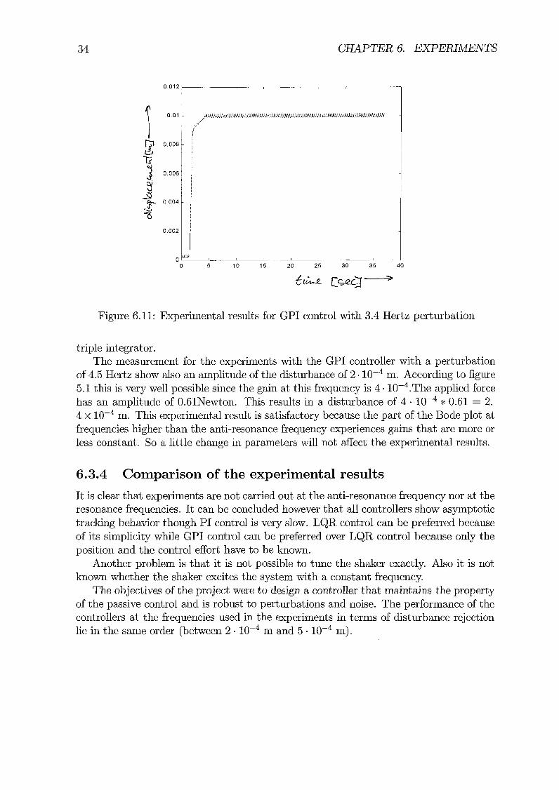
triple integrator. The measurement for the experiments with the GPI controller with a perturbation
of 4.5 Hertz show also an amplitude of the disturbance of 2 . lop4 m. According to figure 5.1 this is very well possible since the gain at this frequency is 4 . 1OW4.The applied force has an amplitude of 0.61Newton. This results in a disturbance of 4 lop4 * 0.61 = 2. 4 x lop4 m. This experimental result is satisfactory because the part of the Bode plot at frequencies higher than the anti-resonance frequency experiences gains that are more or less constant. So a little change in parameters will not affect the experimental results.
6.3.4 Comparison of the experimental results
It is clear that experiments are not carried out at the anti-resonance frequency nor at the resonance frequencies. It can be concluded however that all controllers show asymptotic tracking behavior though PI control is very slow. LQR control can be preferred because of its simplicity while GPI control can be preferred over LQR control because only the position and the control effort have to be known.
Another problem is that it is not possible to tune the shaker exactly. Also it is not known whether the shaker excites the system with a const ant frequency.
The objectives of the project were to design a controller that maintains the property of the passive control and is robust to perturbations and noise. The performance of the controllers at the frequencies used in the experiments in terms of disturbance rejection lie in the same order (between 2 . loW4 m and 5 . loW4 m).

Chapter 7
Conclusions and recommendations
The objectives of the project were to design a controller that maintains the anti resonance property of the passive control and is robust to perturbations and noise. GPI is the only control strategy in comparison with PI and LQR that, in theory, is robust to noise and preserves the anti resonance of the passive absorber. Also in the simulations shows GPI the best performance. It should be noted that more control strategies are available that possibly are simpler to implement and possibly perform better than GPI control.
A disadvantage of the GPI control is that it is a complicated controller to build. Also experimentally do errors in the initial conditions blow up to make the system instable. LQR shows good results in simulation however it does not conserve the anti resonance property of the vibration absorber. PI control preserves the property of the anti resonance of the vibration absorber but the gain at the resonance frequencies is still very large. Also the PI controller is not suitable since the system is underactuated. This however is not a surprise since PI is not a good control strategy on the fourth order mass-spring-damper system. PI is a very successful strategy on lower order systems. The conclusions that can be drawn from theory and simulation can not be justified by the experiments. More experiments are necessary.
It is possible to obtain better results, therefore some recommendations are made. In order to be able to make a comparison between the experimental and the simulation results it is necessary to use the same parameters in simulations and experiments. Also it is useful to use a shaker that excites the system with a constant frequency and that is easily adjustable to another frequency without the need to decouple the system. The measurements that are needed for the controllers to work enter the ECPTM programs in counts. It is recommended that the inputs are first converted to meters and Newtons before the control is executed. This control should be computed in Newtons, while the control force that is send to the DC motor is modified with a factor called the hardware gain. With these recommendations it should be possible to obtain better results.
Appendix A
K 131 n - r &A-mes: r lfindgain
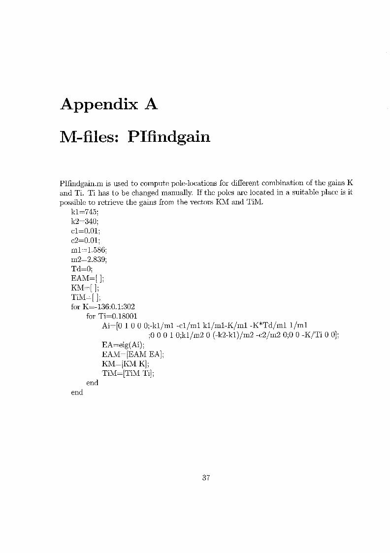
P1findgain.m is used to compute pole-locations for different combination of the gains K and Ti. Ti has to be changed manually. If the poles are located in a suitable place is it possible to retrieve the gains from the vectors KM and TIM.
kl=745; k2=340; cl=O.Ol; c2=0.01; mL=1.586; m2=2.839; Td=O; EAM= [ ] ; KM=[ 1; TIM= [ ] ; for K=-136:0.1:302
for Ti=0.18001 Ai=[O 1 0 0 0;-kl/ml -cl/ml kl/ml-K/ml -K*Td/ml l / m l
;O 0 0 1 O;kl/m2 0 (-k2-kl)/m2 -c2/m2 0;O 0 -K/Ti 0 01; EA=eig(Ai) ; EAM= [EAM EA] ; KM=[KM K] ; TIM= [TIM Tij ;
end end
Appendix B
1. -1 Simulmt model: Passive control
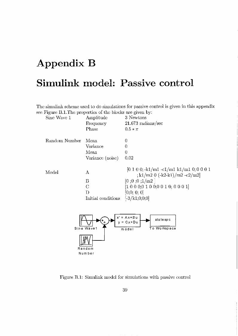
The simulink scheme used to do simulations for passive control is given in this appendix see Figure B.1.The properties of the blocks are given by:
Sine Wave 1 Amplitude 3 Newtons Frequency 21.673 radianslsec Phase 0.5 * ir
Random Number Mean 0 Variance 0 Mean 0 Variance (noise) 0.02
Model A (0 1 0 0; -kl/ml -cl/ml k l /ml 0; 0 0 0 1
; kl/m2 0 (-k2-kl)/m2 -c2/m2] B [0 ;O ;O ;l/m2 ] C [I 0 0 0;o 1 0 O;o 0 1 0; 0 0 0 11 D [O;O; 0; 01 Initial conditions [-3/k1;0;0;0]
w R a n d o m
x ' = A x + B u y = Cx+Du
N u m b e r
Figure B.l: Simulink model for simulations with passive control
39
S i n e Wave1 m ode1 T o Workspace
--b statesp c
0 (asrou ou) uzan ~aqumu mopuq
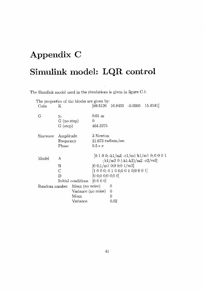
APPENDIX C. SIMULINK MODEL: LQR CONTROL
Number
Figure C.l: Sirnulink model for LQR control

Appendix D
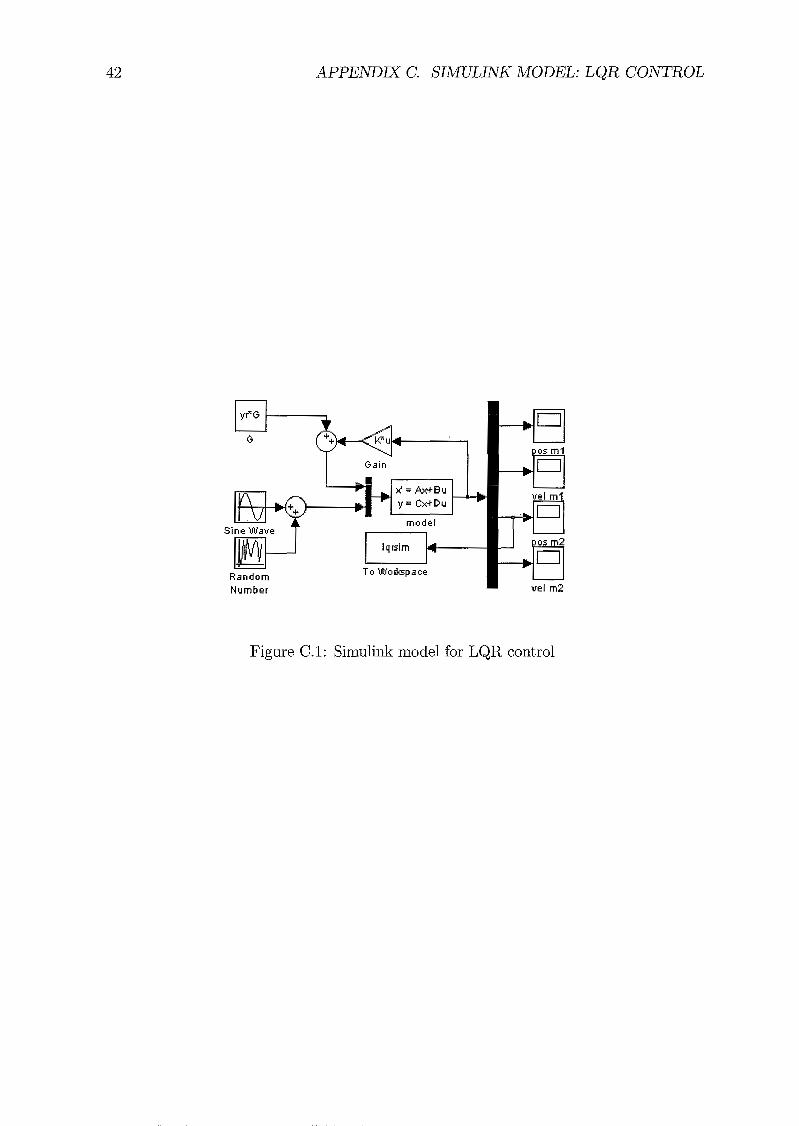
1 1 Sirnulink moaels: PI control
The simulirik model that is used for the PI control can be found in figure D.1. The properties of the blocks are given by:
PID
S me ' wave
Random number
Constant
Model
Amplitude 3 Newton Frequency 21.673 radianslsec Phase 0.5 * .i.r
Mean (no noise) 0 Variance (no noise) 0 Mean 0 Variance 0.02
C (no step) 0 C 0.01
A [0 1 0 0;-kl/ml -cl/ml k l /ml 0;O 0 0 11
;kl/m2 0 (-kl-k2)/m2 -c2/m2 B [0 O;i/mi 0;O 0;O -i/m2] C [o 0 1 01 D 10 01 Initial conditions [ 0 0 0 01
APPENDIX D. SIMULINK MODELS: PI CONTROL
W B c ! 1 y = C*Du
State-Space
Sine W a r e I I E i n A U pidsim L 4 - l Random Number
Figure D. 1: Simulation model for PI control
Appendix E
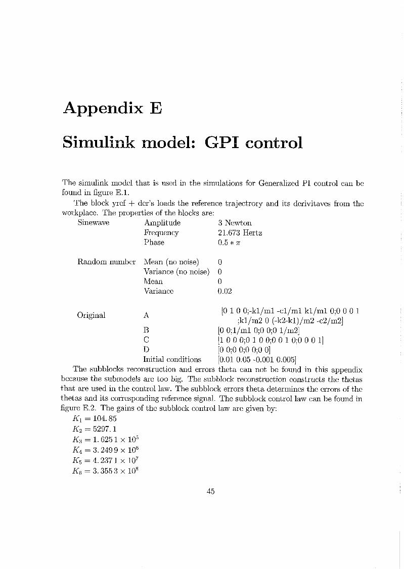
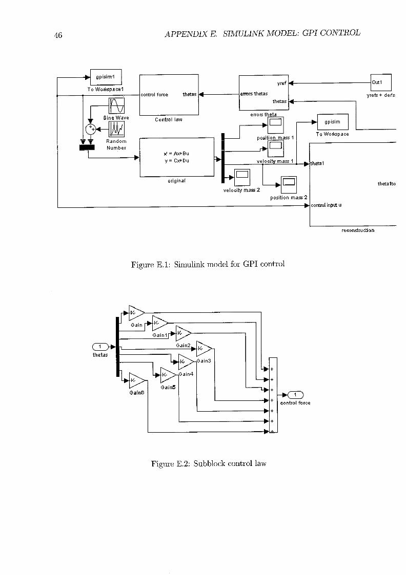
Sirnulink model: GPI control
The simulink model that is used in the simulations for Generalized PI control can be found in figure E. 1.
The block yref + der's loads the reference trajectrory and its derivitaves from the workplace. The properties of the blocks are:
S' mewave
Random number
Original
Amplitude 3 Newton Frequency 21.673 Hertz Phase 0.5 * .i7
Mean (no noise) 0 Variance (no noise) 0 Mean 0 Variance 0.02
A [0 1 0 0;-kl/ml -cl/ml k l /ml 0;O 0 0 1
;kl/m2 0 (-k2-kl)/m2 -c2/m2] B [0 O;l/ml 0;o 0;o l/m2] C [l 0 0 0;o 1 0 0;o 0 1o ;o 0 0 I] D [O O;o 0;o 0;o 01 Initialconditions [0.010.05-0.0010.005]
The subblocks reconstruction and errors theta can not be found in this appendix becaduse the submodels are too big. The subblock reconstruction constructs the thetas that are used in the control law. The subblock errors theta determines the errors of the thetas and its corresponding reference signal. The subblock control law can be found in figure E.2. The gains of the subblock control law are given by:
Kl = 104.85 K2 = 5297.1 K3 = 1.625 1 x lo5 K4 = 3.249 9 x lo6 K5 = 4.237 1 x lo7 K6 = 3.3553 x lo8
Sine Wave
Number
APPENDIX E. SIMULINK MODEL: GPI CONTROL
control force thetas
Control law
yref 4 -
errors t h k
p o s i t i a n m a I
-b 2 = W B U - y = Cx+Du =b velocity m a s I - ,, -
original -
Out1
velocity mars 2 -u position m a s 2
4 errors thetas -
yrefs+ der's thetas f
:hetal
mntrol input u
thetalto
reconstruction
Figure E. 1: Sirnulink model for GPI control
Figure E.2: Subblock control law
Appendix F
ECP programs: LQR
This appendix gives the ECPTM-program that is used during the experiments for LQR control.
.*********** variables ................................... >
#define K1 q l #define K2 q2 #define K3 q3 #define K4 q4 #define G q5 #define posoldl q6 #define posold2 q7 #define vell q8 #define ve12 q9 #define deltat q10 #define khw q l l .****** Initialize variables ..................................... >
posoldl=O ;initial value for old position for mass carriage 1 posold2=0 ;initial value for old position for mass carriage 2 vell=O ;initial velocity of mass carriage 1 ve12=0 ;initial velocity of mass carriage 2 deltat=0.000884 ; remember to choose Ts=0.000884 in dialog box prior
; to !'Implement !' khw=12000 ;hardware gain (see manual) K1=89.5126 ;gain 1 K2=16.8403 ;gain 2 K3=-6.0366 ;gain 3 K4=15.4141 ;gain 4 G=430 ;value to get system to reference .********** Real-Tirne User Code ***********J"**J"** ;k**** ;k******* 7
begin vell= (encl - pos-posoldl) Ideltat ;construction of the velocity of mass

APPENDIX F. ECP PROGRAMS: LQR
;carriage 1 ve12=(enc2~pos-posold2)/deltat ;construction of the velocity of mass
;carriage 2 control - effort=(l/khw)* (-Kl*(encl-pos)-K2*vell
-K3*(enc2 - pos)-K4*vel2+G*cmd-pos) posoldl=encl -pas posold2=enc2-pos
end
Appendix G
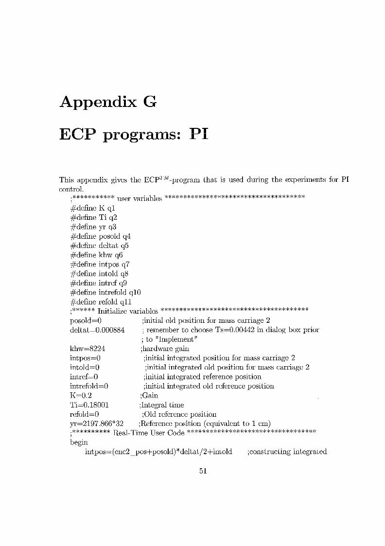
l7n P programs: PI
This appendix gives the ~ C ~ ~ " - ~ r o g r a m that is used during the experiments for PI control.
.*********** variables ..................................... 1
#define K q l #define Ti q2 #define yr q3 #define posold q4 #define deltat q5 #define khw q6 #define intpos q7 #define intold q8 #define intref q9 #define intrefold q10 #define refold q l l .****** Initialize ....................................... 1
posold=O ;initial old position for mass carriage 2 deltat=0.000884 ; remember to choose Ts=0.00442 in dialog box prior
; to "Implement "
khw=8224 ;hardware gain intpos=O ;initial integrated position for mass carriage 2 intoid=O ;initial integrated old position for mass carriage 2 intref=O ;initial integrated reference position intrefo!d=O ;initial. integrated old reference position K=0.2 ;Gain Ti=O. 18001 ;Integral time refold=O ;Old reference position yr=2197.866*32 ;Reference position (equivalent to 1 cm) .********** Real-Tirne User Code .................................. 1
begin intpos=(enc2 - posfposold) *deltat/2+intold ;constructing integrated

APPENDIX G. ECP PROGRAMS: PI
;position intref=yr*deltat +intrefold ;integrated reference
;position control - effort=(l/khw) * (K* (yr-enc2 - pos) +(K/Ti) * (intref-intpos)) int old=intpos ;updating intrefold=intref refold=cmd-pos posold=enc2-pos
end ..............................................................
Appendix H
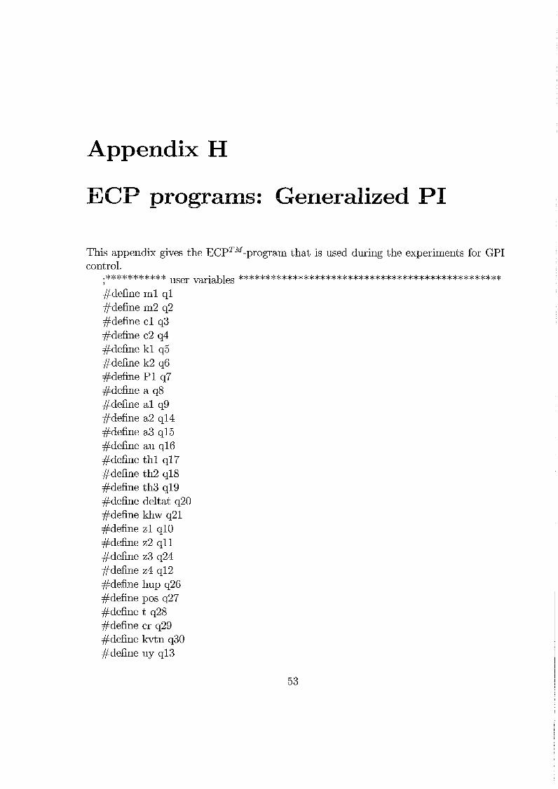
1 n T ECP programs: Generalizes rl
This appendix gives the E C ~ ~ ~ - ~ r o g r a r n that is used during the experiments for GPI control.
.*********** variables ................................................ 1
#define ml q l #define m2 q2 #define c l q3 #def;,r,e c2 q4 #define k l q5 #define k2 q6 #define P I q7 #define a q8 #define a1 q9 #define a2 q14 #define a3 q15 #define au q16 #define th l q17 #define th2 q18 #define th3 q19 #define deltat q20 #define khw q21 #define z l q10 #define 22 q l l #define 23 q24 #define 24 q12 #define hup q26 #define pos q27 #define t q28 #define cr q29 #define kvtn q30 #define uy q13
APPENDIX H. ECP PROGRAMS: GENERALIZED PI
#define uyi q32 #define uyold q33 #define uyiold q34 #define uyiy q35 #define uyiyold q36 #define uyiyi q37 #define uyiyiold q38 #define uyiyiy q39 #define uyiyiyold q40 #define uyiyiyi q41 #define uyiyiyiold q42 #define P2 q43 #define P3 q44 #define P4 q45 #define P5 q46 #define P6 q47 #define P7 q48 #define refdd q49 #define refddd q50 #define refi q5i #define refiold q52 #define refii q53 #define refiiold q54 #define refiii q55 #define refiiiold q56 #define yr q57 #define bO q58 #define bl q59 #define b2 q60 #define b3 q6l #define b4 q62 #define b5 q63 #define b6 q64 #define b7 q65 #define b8 q66 #define b9 q6? #define to q68 #define cr q69 #define td q70 #define d l q71 #define d2 q72 #define d3 q73 #define d4 q74
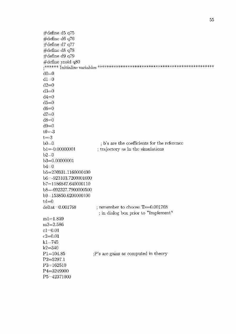
dO=O dl=0 d2=0 d3=0 d4=0 d5=0 d6=0 d7=0 d8=0 d9=0 t 0=-3 t =-3 bO=O bl=-0.00000001 b2=0 b3=0.00000001 b4=0 b5=27693l. ll6OOOO4OO b6=-923103.7200001000 b7=ll86847.64OOOOllO b8=-692327.7900000500 b9=153850.6200000100 td=O delt at =O. 001 768
; b's are the coefficients for the reference ; trajectory as in the simulations
; remember to choose Ts=0.001768 ; in dialog box prior to "Implement"
;P's are gains as computed in theory
APPENDIX H. ECP PROGRAMS: GENERALIZED PI
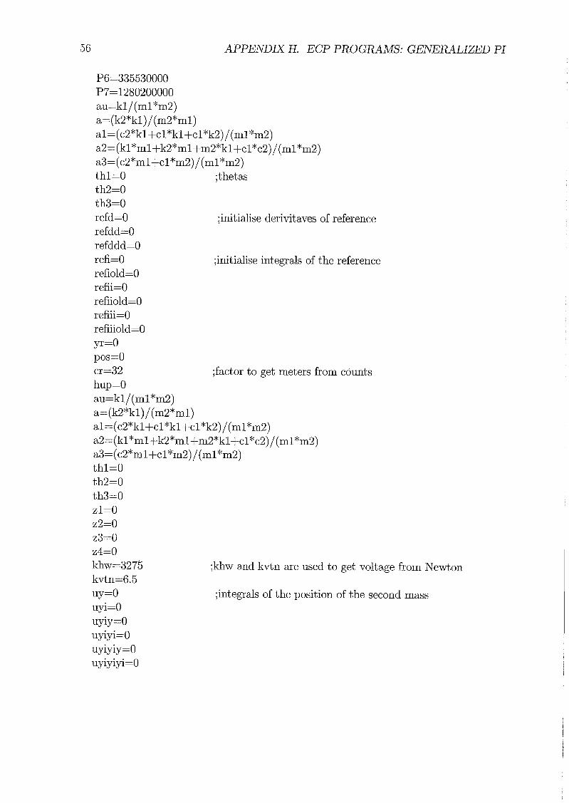
P6=335530000 P7=1280200000 au=kl/(ml*m2) a=(k2*kl)/(m2*ml) al=(c2*kl+cl*kl+cl*k2)/(ml*m2) a2=(kl*ml+k2*ml+m2*kl+cl*c2)/(ml*m2) a3=(c2*ml+cl*m2)/(ml*m2) thl=O ;thetas th2=0 th3=0 refd=O ;initialise derivitaves of reference refdd=O refddd=O refi=O ;initialise integrals of the reference refiold=O refii=O refiiold=O refiii=O refiiiold=O yr=O pos=o cr=32 ;factor to get meters from counts hup=O au=kl/(ml*m2) a=(k2*kl)/(m2*ml) al=(c2*kl+cl*kl+cl*k2)/(ml*m2) a2=(kl*ml+k2*ml+m2*kl+cl*c2)/(ml*m2) a3=(c2*ml+cl*m2)/(ml*m2) thl=O th2=0 th3=0 zl=O z2=0 z3=0 z4=0 khw=3275 kvtn=6.5 uy=o uyi=O uyiy=O uyiyi=O uyiyiy=O uyiyiyi=O
;khw and kvtn are used to get voltage from Newton
;integrals of the position of the second mass
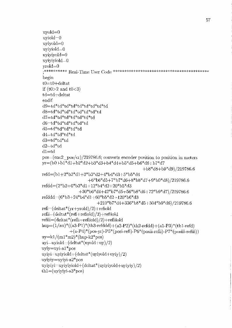
uyold=O uyiold=O uyiyold=O uyiyiold=O uyiyiyold=O uyiyiyiold=O yrold=O .********** Real-Tirne User Code .......................................... 1
begin tO=tO+deltat if (t0>2 and t0<3) td=td+deltat endif d9=td*td*td*td*td*td*td*tdJftd d8=td*td*td*td*td*td*tdJFtd d7=td*td*td*td*td*td*td d6=td*td*td*td*td*td d5=td*td*td*td*td d4=td*td*td*td d3=td*td*td d2=td*td dl=td pos=(enc2 - pos/cr)/219786.6; converts encoder position to position in meters yr=(bO+bl*dl+b2*d2fb3*d3+b4*d4+b5*d5+b6"d6+b7*d7
+b8*d8+b9*d9)/219786.6 refd=(bl+2*b2*d1+3*b3*d2+4*b4*d3+5*b5*d4
+6*b6*d5+7*b7*d6+8*b8*d7+9*b9*d8)/219786.6 refdd=(2*b2+6*b3*dl+12*b4*d2+20*b5*d3
+30*b6*d4+42*b7*d5+56*b8*d6+72*b9*d7)/219786.6 refddd=(6*b3+24*b4*dl+60*b5*d2+120*b6*d3
+210*b7*d4+336*b8*d5+504*b9*d6)/219786.6 refi= (deltat * (yrfyrold) 12) frefiold refii= (deltat * (refi-krefiold) 12) frefiiold re&= (deliat* (refii+refiiold j /2) +refiiiold hup=(l/au) * ((a3-PI) * (th3-refddd) + (a2-P2) * (t h2-refdd) +(al-P3) * (thl-refd)
+ (a-P4) * (pos-yr)-P5* (posi-refi)-P6* (posii-sefii)-P7* (posiii-refiii)) uy=kl/(ml*m2)*(hup-k2*pos) uyi=uyiold+ (delt at * (uyold+uy) 12) uyiy=uyi-al*pos uyiyi=uyiyiold+ (delt at * (uyiyold+uyiy) 12) uyiyiy=uyiyi-a2*pos uyiyiyi=uyiyiyiold+ (delt at * (uyiyiyold+uyiyiy) 12) t h l = (uyiyiyi-a3"pos)

58 APPENDIX H. ECP PROGRAMS: GENERALIZED PI
th2=(uyiyi-a2*pos-a3*thl) th3=(uyi-al*pos-a2*thl-a3*th2) zl=l/kl*(m2*th2+c2*thl+(kl+k2)*pos) z2=l/kl*(m2*th3+ c2*th2+(kl+k2)*thl) z3=pos z4=thl control - effort=hup*khw/kvtn uyold=uy uyiold=uyi uyiyold=uyiy uyiyiold=uyiyi uyiyiyold=uyiyiy uyiyiyiold=uyiyiyi refiold=refi refiiold=refii refiiiold=refiii yrold=yr end ........................................................................
Appendix I
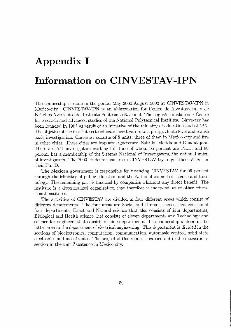
T T Information on CINVESTAk -IPN
The traineeship is done in the period May 2002-August 2002 at CINVESTAV-IPN in Mexico-city. CINVESTAV-IPN is an abbreviation for Centro de Investigacion y de Estudios Avanzados del Instituto Politecnico National. The english translation is Centre for research and advanced studies of the National Polytecnical Institute. Cinvestav has been founded in 1961 as result of an initiative of the ministry of education and of IPN. The objctive of the institute is to educate investigators to a postgraduate level and realise basic investigacion. Cinvestav consists of 8 units, three of them in Mexico city and five in other cities. These cities are Irapuato, Queretaro, Saltillo, Merida and Guadalajara. There are 571 investigators working full time of whom 95 percent are Ph.D. and 80 percent has a membership of the Sistema Nacional of Investigators, the national union of investigators. The 2000 students that are in CINVESTAV try to get their M. Sc. or their Ph. D.
The Mexican government is responsible for financing CINVESTAV for 95 percent through the Ministry of public education and the National council of science and tech- nology. The remaining part is financed by companies whithout any direct benefit. The institute is a decentralized organization that therefore is independant of other educa- tional institutes .
The activities of CINVESTAV are divided in four different areas which consist of different departments. The four areas are Social and Human science that consists of four departments, Exact and Natural science that also consists of four departments, Biological and Health science that consists of eleven departments and Technology and science for engineers that consists of nine departments. The traineeship is done in the latter area in the department of electrical engineering. This department is divided in the sections of bioelectronics, computation, communication, a~tomatic control, solid state electronics and mecatronics. The project of this report is carried out in the mecatronics section in the unit Zacatenco in Mexico city.
Bibliography
Parks, T.R., " Manual for model 210/210a, rectilinear control system", 1999, Edu- cational Control Products.
Rao, S.S., "Mechanical vibrations", third edition, Addison-Wesley: 1995
Datta, A, Ho, M.T. and bhattacharyya, S.P., "Structure and synthesis of PID controllers", 2000, Springer-Verlag, London
Astrom, A. J. and Hagglund, T , "PID controllers: theory design and tuning", 1995, International Society for Measurement and Control, Research Triangle Park, NC.
Yu, C.C. "Autotuning of PID controllers", 1999, Springer-Verlag, London.
Lewis, F.L., "Applied Optimal Control and Estimation: digital design and imple- mentation", 1992, Prentice-Hall, NJ.
Franklin, G.F., Powell, J.D. and Workman, M.L., "Digital control of dynamic sys- tems", 1990, Addison-Wesley, NY.
Van Brussel, H., Sas, P, Dehandschutter, W., Van den Braembussche, P and In- drawanto, "New methods for active and semi-act ive vibration control in machines", Leuven.
Herzog, R, "Active versus passive vibration absorbers", Journal of dynamic systems, measurement and control, september 1994, Vo1.116, 367-371, Zurich.
[lo] Vazquez, B, Silva, G and Alvarez, J, "Active vibration control of an oscillating rigig bar using nonlinear output regulation techniques", SPIE Vol. 3989, Damping and isolation, march 2000, D.F. Mexico.
[Ill Vazquez , B, Silva, G and Alvarez, J , "A nonlinear vibration absorber based on nonlinear control methods", D.F. Mexico.
[12] Fliess, M, Marquez, R, Delaleau, E and Sira-Ramirez, H, "Correcteurs proportionnels-integraux generalises I' , 2002, ESAIM: Control, Optimization and calculus of variations, Vol. 7, pp. 23-41.

62 BIBLIOGRAPHY
1131 Belt ran- Carbaj al, F., Silva-Navarro, G . and Sira-Ramirez, H, I' Passive and active vibration absorbers using generalized PI control", D.F. Mexico.
[14] Hernandez, V.M. and Sira-Ramirez, H, "Position control of an inertia-spring DC- motor system without mechanical sensors: experiment a1 results", 2001, IEEE, p.p. 1386-1391, D.F. Mexico.