Noise Increases Anchoring Effects Chang-Yuan Lee and Carey

Noise Increases Anchoring Effects


Chang-Yuan Lee and Carey K. Morewedge

Boston University

In press at Psychological Science.


2

Abstract

We introduce a theoretical framework distinguishing between anchoring effects, anchoring bias,

and judgmental noise: Anchoring effects require anchoring bias, but noise modulates their size.

We test it by manipulating stimulus magnitudes. As magnitudes increase, psychophysical noise

due to scalar variability widens the perceived range of plausible values for the stimulus. This

increased noise, in turn, increases the influence of anchoring bias on judgments. In eleven

preregistered experiments (N = 3,552), anchoring effects increased with stimulus magnitude for

point estimates of familiar and novel stimuli (e.g., reservation prices for hotels and donuts,

counts in dot arrays). Comparisons between relevant and irrelevant anchors showed noise itself

did not produce anchoring effects. Noise amplified anchoring bias. Our findings identify a

stimulus feature predicting the size and replicability of anchoring effects––stimulus magnitude.

More broadly, we show how to use psychophysical noise to test relationships between bias and

noise in judgment under uncertainty.

Keywords: anchoring bias, noise, judgment under uncertainty, numerical cognition


3

An anchoring effect occurs when considering one number, an anchor, leads subsequent

estimates to be assimilated to it. Anchoring effects occur in judgments ranging from mundane

trivia answers to the selling price of homes, but are not ubiquitous (Northcraft & Neale, 1987;

Tversky & Kahneman, 1974). Anchoring effects vary in size across anchors and judges and

contexts (Jacowitz & Kahneman, 1995; Jung, Perfecto, & Nelson, 2016; Smith, Windschitl, &

Bruchmann, 2013; Wilson, Houston, Etling, & Brekke, 1996). We propose that noise in the

mental representation of the stimulus estimated (i.e., the target) is a critical determinant of the

size of anchoring effects.

We base our theoretical framework on the anchoring-and-adjustment-heuristic (Epley &

Gilovich, 2006; Simmons, LeBoeuf, & Nelson, 2010; Tversky & Kahneman, 1974). It posits that

people estimate the value of a target (e.g., the duration of Mars’ orbit) by identifying an anchor

(e.g., Earth’s orbit = 365 days). People then adjust from that anchor until they reach a range of

plausible values for the point estimate and stop at a value within that range. Because adjustment

is usually insufficient (i.e., people typically stop at a value before rather than beyond the correct

answer), estimates are biased by consideration of anchors (Quattrone, Lawrence, Finkel, &

Andrus, 1984). The average estimate of Mars’ orbit is 492 days, for instance, which is 195 days

less than the right answer (i.e., 687 days; Epley & Gilovich, 2006).

“Anchoring effect” and “anchoring bias” are used interchangeably to describe this

biasing effect of anchors (e.g., Chapman & Johnson, 1994; Englich, Mussweiler, & Strack, 2006;

Epley & Gilovich, 2006), but errors in judgment are driven by both bias and noise (Kahneman,

Rosenfield, Gandhi, & Blaser, 2016). We propose the terms should be distinct, as anchoring

effects are also a product of bias and noise. Most anchoring research examines an anchoring

effect, which we define as the absolute effect of an anchor on an estimate. It can be calculated as


4

the raw difference between point estimates influenced by low and high anchors, or the raw

difference between point estimates made with and without an anchor. The anchoring effect

indicated by the red line in Example A/Figure 1 is the raw difference between point estimates

made with low and high anchors, AL and AH.

Figure 1. In Examples A, B, and C, the (absolute) anchoring effects of low and high anchors on

point estimates are smallest in Example A (AH - AL), and equally larger in Examples B and C (BH

- BL; CH - CL). Anchoring bias is greatest in Example C where there is the least (relative)

correction from anchors, and equally smaller in Examples A and B. Noise is greatest in Example

B, which has the widest plausible range of stimulus values, and equally smaller in Examples A

and C. Black arrows depict adjustment from low and high anchors to the range of plausible

values of the point estimate.


5

Noise in our framework reflects the width of the range of plausible values for the point

estimate, the distance between the minimum and maximum plausible values. It is essentially the

judge’s subjective confidence interval. The red line in Example C/Figure 1 indicates the

plausible range width for point estimates CL and CH.

Anchoring bias is the degree of undercorrection from the anchor in the point estimate,

relative to the range of plausible values. In Example B/Figure 1, judges corrected only halfway

from plausible extremums to the midpoint in point estimates BL and BH. Anchoring bias can be

measured with a skew index (Epley & Gilovich, 2006) dividing the (a) difference between a

point estimate and the plausible extremum nearest to the anchor (low anchor à minimum

plausible value; high anchor à maximum plausible value), by (b) the difference between the

minimum and maximum plausible value (see Experiment 6A for details). Thus, the same

anchoring bias produces a smaller anchoring effect when there is less noise, and a larger

anchoring effect when there is more noise.

Our framework shows how noise and anchoring bias together determine the size of

anchoring effects. Furthermore, it helps specify whether anchoring effects vary across factors

like judges, anchors, and contexts because they modulate anchoring bias or noise. We illustrate

these proposals in Figure 1. An expert (Example A) and novice (Example C) could be equally

uncertain about the plausible value of a stimulus (same noise), but the expert exhibits a smaller

anchoring effect than the novice because she is less biased by the anchor (less anchoring bias).

Alternatively, the expert (Example A) could be as biased by the anchor as the novice (Example

B; same anchoring bias), but she exhibits a smaller anchoring effect because the range of

plausible values she considers is narrower than the range the novice considers (less noise).


6

We test our theory by manipulating anchors and stimulus magnitudes. Scalar variability

makes mental representations of numbers nosier as stimulus magnitudes increase (Feigenson,

Dehaene, & Spelke, 2004). The range of plausible values for point estimates should then widen

with stimulus magnitude. The range between the minimum and maximum plausible weight of a

small dog, for instance, should be narrower than the range between the minimum and maximum

plausible weight of a large dog. We test this prediction in six pretests. Consequently, anchoring

effects should increase with stimulus magnitude, even when anchoring bias is similar in

estimates of smaller and larger targets (we test this in Experiments 6A and 6B).

We test if anchoring effects increase with stimulus magnitude in Experiments 1A-3B. In

Experiments 4A and 4B, we test if low stimulus magnitudes explain cases where anchoring

effects are weak or have failed to replicate (Jung et al., 2016; Maniadis et al., 2014). In

Experiment 5, we test the proposed relationship between anchoring effects, anchoring bias, and

noise. In Experiments 6A and 6B, we directly compare effects of stimulus magnitude on

anchoring effects, anchoring bias, and noise.

Open Practices Statement

All experiments were preregistered on AsPredicted (see SOM for preregistrations). We

report how we determined our sample size, all data exclusions (if any), all manipulations, and all

measures in all experiments. All data are available at:

https://osf.io/9xun6/?view_only=4ec11927192d451489de206954fc6d82

Pretests: Plausible Range Widths by Stimulus Magnitudes

In six categories of stimuli, we tested if the plausible range of stimulus values widen as

stimulus magnitudes increase.

Method


7

Miami Hotels. We recruited 50 participants from Amazon Mechanical Turk to be well

powered to detect medium sized effects within-subjects, and 50 AMT workers completed the

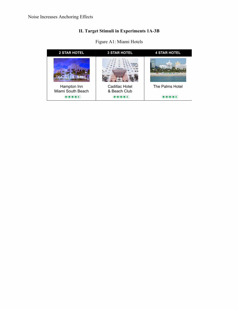
pretest. Participants saw pictures of three hotels in Miami Beach, Florida vertically differentiated

by star rating (i.e., a 2-star hotel, a 3-star hotel, and a 4-star hotel; Figure A1). In open-ended

response boxes, participants estimated the highest and lowest market price ($USD per night) of a

standard room in each hotel in the past year.

Dog Breeds. We recruited 50 participants from Amazon Mechanical Turk, and 48 AMT

workers completed the pretest. Participants saw pictures of three adult dogs of different breeds,

which they were told varied in size from small to medium to large (i.e., Basenji, American

Staffordshire Terrier and Bernese Mountain Dog, respectively; Figure A2). In open-ended

response boxes, participants estimated the maximum and minimum plausible weight in pounds

of each of the three dog breeds.

French Fries. We recruited 50 participants from Amazon Mechanical Turk, and 52 AMT

workers completed the pretest. Participants saw pictures of small, medium, and large servings of

McDonald’s French Fries (Figure A3). In open-ended response boxes, participants estimated the

maximum and minimum plausible number of calories in each serving.

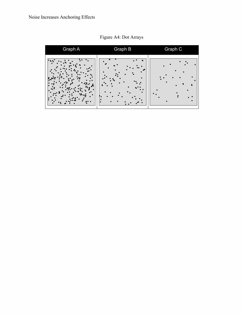
Dot Arrays. We recruited 50 participants from Amazon Mechanical Turk, and 50 AMT

workers completed the pretest. Participants saw pictures of three dot arrays that obviously varied

in the number of dots each contained (i.e., 35, 97 and 273 dots, Figure A4). In open-ended

response boxes, participants estimated the maximum and minimum plausible number of dots in

each of the three arrays.

Donuts. We recruited 50 participants from Amazon Mechanical Turk, and 50 AMT

workers completed the pretest. Participants were first presented with an image of Dream Fluff


8

Donuts, adapted from Jung and colleagues (2016). In open-ended response boxes, participants

estimated the highest and lowest market price for one donut and for one dozen donuts made by

Dream Fluff Donuts’.

Unpleasant Tones. We recruited 50 participants from Amazon Mechanical Turk, and 50

AMT workers completed the pretest. Participants first listened to an unpleasant tone for 30

seconds, the same tone used by Maniadis and colleagues (2014). Participants then read that other

100 AMT workers had reported the maximum amount of money they were willing to accept

(WTA) to listen to the same tone for 60, 180, and 300 seconds. In open-ended response boxes,

participants estimated the highest and lowest amounts of money that those AMT workers

requested to listen to the tone for each of the three durations.

Results

We first computed plausible range widths for each stimulus, within each participant, by

subtracting the minimum estimate from the maximum estimate; mean plausible range widths and

standard deviations are reported in Table 1. We then compared the widths of plausible ranges for

the largest, medium, and smallest magnitude stimuli. As predicted, the mean plausible range of

the largest magnitude stimulus was wider than the plausible range of the medium and smallest

magnitude stimuli (all ts ≧ 2.16, all ps ≦ .036, all ds ≧ .31), and the plausible range of the

medium magnitude stimulus was wider than that of the smallest magnitude stimulus (all ts ≧

2.75, all ps ≦ .008, all ds ≧ .39). For all comparisons, see Supplemental Online Materials.


9

Table 1.

Plausible Range Width by Stimulus Magnitude in Pretests

Stimulus Magnitude

Stimuli Small Medium Large

Miami Hotels ($USD / per night)

Δ89.26 (102.01)a Δ115.94 (90.56)b Δ144.22 (115.33)c

Dog Breeds (lbs.)

Δ29.40 (18.48)a Δ53.77 (48.94)b Δ74.75 (51.88)c

French Fry Servings (calories) Δ81.98 (119.79)a Δ117.00 (178.96)b Δ156.38 (254.52)c

Dot Arrays (counts)

Δ21.64 (13.29)a Δ40.06 (29.97)b Δ118.20 (148.95)c

Donuts ($USD)

Δ1.75 (1.94)a - Δ5.77 (5.39)b

Unpleasant Tones ($USD)

Δ3.24 (5.08)a Δ4.73 (6.51)b Δ7.38 (9.37)c

Note. Means within rows that do not share subscripts differ at p < .05 in paired sample t-tests

(within-subjects). Standard deviations in parentheses.


10

Experiments 1A-3B: Directional Tests

Given that plausible ranges of stimulus values widen with stimulus magnitude, our theory

predicts that anchoring effects should increase with stimulus magnitude. To compare across

subjective and objective judgments, we operationalized anchoring effects as the difference in

point estimates between participants exposed to a low anchor, high anchor, or no anchor

(depending on experiment). In Experiments 1A and 1B, we manipulated externally provided

anchors between-subjects and targets within-subjects. In Experiments 2A and 2B, we

manipulated internally generated anchors between-subjects and targets within-subjects. In

Experiments 3A and 3B, we manipulated externally provided anchors and targets between-

subjects.

Experiment 1A: WTP for Miami Hotels

Method

Participants and Design

We requested 300 participants from Amazon Mechanical Turk; 297 AMT workers

completed Experiment 1A (39% female; Mage = 36.40 years; SD = 10.43). Generally, we aimed

to recruit at least 100 participants per condition in our experiments as the focal statistical

predictions were interaction effects. In a mixed design, we randomly assigned participants,

between-subjects, to one of three externally provided anchoring conditions: control (i.e., no

anchor), low anchor, or high anchor. Each participant then reported her willingness-to-pay

(WTP) for three Miami hotels (within-subjects).

Procedure

In the no anchor condition, participants saw no anchor. They imagined purchasing a hotel

room for one night during an upcoming trip to Miami, and were presented with the name, a


11

photograph, TripAdvisor traveler rating, and star rating for each of three Miami Beach hotels

(i.e., a 2-star hotel, a 3-star hotel, and a 4-star hotel). Participants then reported their maximum

WTP in $USD for a room for one night in an open response box, for each of the three hotels.

Values for all three hotels were elicited simultaneously on one survey page.

In the low (external) anchor condition, participants were first informed of the price of a

room for one night in a 1-star Miami Beach hotel (i.e., priced at $44 USD). In the high (external)

anchor condition, participants were first informed of the price of a room for one night in a 5-star

Miami Beach hotel (i.e., priced at $610 USD). Participants then reported their maximum WTP

for a room (per night) for each of the three hotels, just as controls.

Results

To test our directional predictions, we first examined WTP for the three target hotels in a

3 (anchor: no, low, high; between-subjects) × 3 (hotel: 2-star, 3-star, 4-star; within-subjects)

mixed ANOVA, which revealed a significant main effect of anchor (F(2, 294) = 37.37, p < .001,

ηp2 = .20), and a significant main effect of hotel (F(1, 294) = 317.44, p < .001, ηp2 = .52). More

important, these main effects were qualified by a significant anchor × hotel interaction (F(2, 294)

= 34.18, p < .001, ηp2 = .19). Note that, in all mixed and within-subject analyses in this paper, we

report the lower-bound (i.e., the most conservative) estimates. Means and standard deviations are

reported in Figure 2 and Table A1.

We decomposed the interaction with comparisons across each pair of conditions in

separate mixed ANOVAs. Most important, comparing the low and high anchor conditions

revealed a significant 2 (anchor: low, high) × 3 (hotel: 2-star, 3-star, 4-star) interaction (F(1, 192)

= 51.23, p < .001, ηp2 = .21). Simple comparisons showed that participants were willing to pay

more for the 4-star hotel in the high anchor condition than in the low anchor condition (t(192) =


12

9.29, 95% CI = [144.53, 222.44], p < .001, d = 1.33). Participants were also willing to pay more

for the 2-star hotel in the high anchor condition than in the low anchor condition (t(192) = 4.55,

95% CI = [35.75, 90.51], p < .001, d = .65). Moreover, a 2 (anchor: low, high) × 2 (hotel: 2-star,

4-star) interaction revealed that this difference between conditions was significantly greater for

the 4-star than the 2-star hotel (F(1, 192) = 59.08, p < .001, ηp2 = .24; Nieuwenhuis, Forstmann,

& Wagenmakers, 2011).

Comparing the no anchor and high anchor conditions revealed a significant 2 (anchor: no,

high) × 3 (hotel: 2-star, 3-star, 4-star) interaction (F(1, 199) = 31.72, p < .001, ηp2 = .14). Simple

comparisons showed that participants were willing to pay more for the 4-star hotel in the high

anchor condition than in the no anchor condition (t(199) = 6.61, 95% CI = [93.19, 172.45], p

< .001, d = .93). Participants were also willing to pay more for the 2-star hotel in the high anchor

condition than in the no anchor condition (t(199) = 2.33, 95% CI = [5.09, 61.75], p = .021, d

= .33). Moreover, 2 (anchor: no, high) × 2 (hotel: 2-star, 4-star) interaction revealed that the

difference between conditions was significantly greater for the 4-star than the 2-star hotel (F(1,

199) = 38.26, p < .001, ηp2 = .16).

Comparing the no anchor and low anchor conditions revealed a marginal 2 (anchor: no,

low) × 3 (hotel: 2-star, 3-star, 4-star) interaction (F(1, 197) = 3.48, p = .06, ηp2 = .02). Simple

comparisons showed that participants were willing to pay less for the 4-star hotel in the low

anchor condition than in the no anchor condition (t(197) = 3.90, 95% CI = [25.04, 76.30], p

< .001, d = .55). Participants were also willing to pay less for the 2-star hotel in the low anchor

condition than in the no anchor condition (t(197) = 2.40, 95% CI = [5.29, 54.13], p = .017, d

= .34). Moreover, a 2 (anchor: no, low) × 2 (hotel: 2-star, 4-star) interaction revealed that this


13

difference between conditions was significantly greater for the 4-star than the 2-star hotel (F(1,

197) = 4.33, p = .039, ηp2 = .02).

Experiment 1B: Weight of Dog Breeds

Method


We requested 200 participants from Amazon Mechanical Turk. 201 AMT workers

completed Experiment 1B (43% female; Mage = 37.03 years; SD = 11.49). In a mixed design, we

randomly assigned participants to a low or high externally provided anchor (between-subjects).

Each participant then made weight estimates for three dog breeds (within-subjects).

Procedure

Participants randomly assigned (between-subjects) to a low (external) anchor condition

first saw a picture of an adult Australian Terrier and were told that the average weight of its

breed is 12 pounds. In the high (external) anchor condition, participants first saw a picture of an

adult Boerboel and read that the average weight of its breed is 200 pounds. In open-ended

response boxes appearing on the same page, participants then estimated the average weight, in

pounds, of an adult Basenji, an American Staffordshire Terrier (AST), and a Bernese Mountain

Dog (BMD). A picture of each dog accompanied the breed name. The ranking of the weights of

the dog breeds was made explicit. In the low anchor condition, participants saw the ranking:

Australian Terrier < Basenji < American Staffordshire Terrier < Bernese Mountain Dog. In the

high anchor condition, they saw the ranking: Basenji < American Staffordshire Terrier < Bernese

Mountain Dog < Boerboel.


14

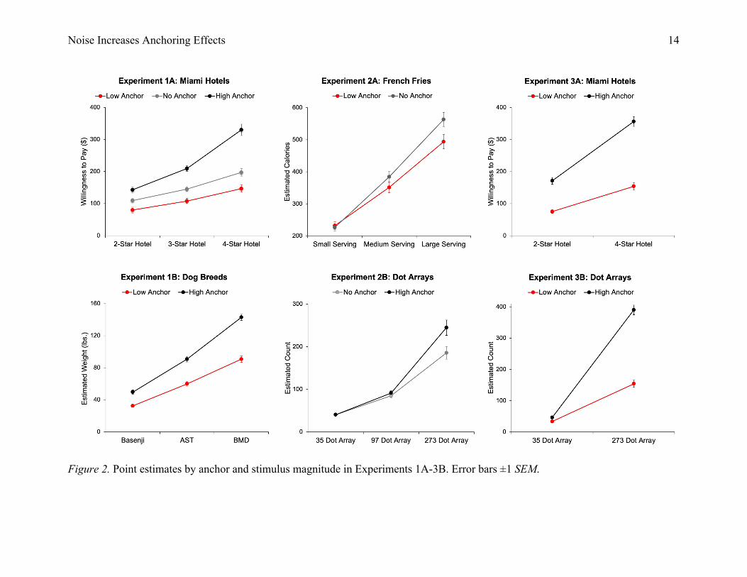
Figure 2. Point estimates by anchor and stimulus magnitude in Experiments 1A-3B. Error bars ±1 SEM.


15

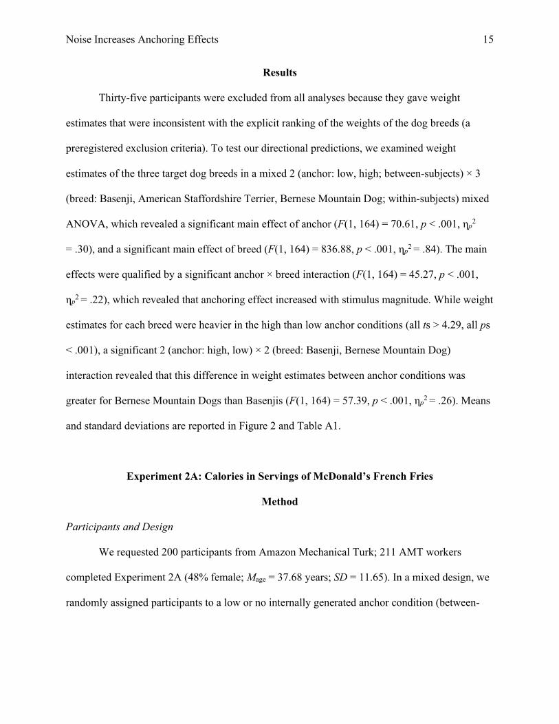
Results

Thirty-five participants were excluded from all analyses because they gave weight

estimates that were inconsistent with the explicit ranking of the weights of the dog breeds (a

preregistered exclusion criteria). To test our directional predictions, we examined weight

estimates of the three target dog breeds in a mixed 2 (anchor: low, high; between-subjects) × 3

(breed: Basenji, American Staffordshire Terrier, Bernese Mountain Dog; within-subjects) mixed

ANOVA, which revealed a significant main effect of anchor (F(1, 164) = 70.61, p < .001, ηp2

= .30), and a significant main effect of breed (F(1, 164) = 836.88, p < .001, ηp2 = .84). The main

effects were qualified by a significant anchor × breed interaction (F(1, 164) = 45.27, p < .001,

ηp2 = .22), which revealed that anchoring effect increased with stimulus magnitude. While weight

estimates for each breed were heavier in the high than low anchor conditions (all ts > 4.29, all ps

< .001), a significant 2 (anchor: high, low) × 2 (breed: Basenji, Bernese Mountain Dog)

interaction revealed that this difference in weight estimates between anchor conditions was

greater for Bernese Mountain Dogs than Basenjis (F(1, 164) = 57.39, p < .001, ηp2 = .26). Means

and standard deviations are reported in Figure 2 and Table A1.

Experiment 2A: Calories in Servings of McDonald’s French Fries

Method



completed Experiment 2A (48% female; Mage = 37.68 years; SD = 11.65). In a mixed design, we

randomly assigned participants to a low or no internally generated anchor condition (between-


16

subjects). Each participant then made calorie estimates for three servings of McDonald’s French

Fries (within-subjects).

Procedure.

At the beginning of the experiment, all participants were told that McDonald’s offered

four different servings of French fries: kids, small, medium, and large. In the no anchor

condition, participants saw pictures of three different servings of McDonald’s French Fries (i.e.,

small, medium, and large) and estimated the number of calories in each serving on the same

page. On a separate page, they next saw a picture of a serving of McDonald’s kids French Fries

and estimated the number of calories in that serving. Participants in the low (internal) anchor

condition first saw and estimated the calories contained in the serving of kids French Fries. They

then saw and estimated the calories contained in small, medium, and large servings. Calorie

estimates were made in open-ended response boxes.

Finally, participants indicated whether they searched online for the calorie information

when estimating the numbers of calories in McDonald’s French fries.

Results

Fourteen participants who reported searching online for the calorie information were

excluded from the analysis (this exclusion criteria was preregistered).

Anchors. Calorie estimates for the kids French Fries serving were significant higher in the

low anchor condition (M = 184.04, SD = 108.24) than in the no anchor condition (M = 150.11,

SD = 78.11, t(195) = 2.52, 95% CI = [7.38, 60.47], p = .01, d = .36).

Targets. To test our directional predictions, we examined calorie estimates for the three

adult sized servings in a 2 (anchor: no, low; between-subjects) × 3 (serving size: small, medium,

and large; within-subjects) mixed ANCOVA with calorie estimate for kids French Fries as a


17

covariate. It revealed a significant main effect of anchor (F(1, 194) = 24.36, p < .001, ηp2 = .11)

and a main effect of serving size (F(1, 194) = 76.60, p < .001, ηp2 = .28). More important, there

was a significant anchor × serving size interaction (F(1, 194) = 23.90, p < .001, ηp2 = .11). The

anchor × serving size interaction holds when calorie estimates for kids French Fries are not

included as a covariate (F(1, 195) = 11.36, p = .001, ηp2 = .06).

Simple comparisons showed that calorie estimates for the large serving were significantly

lower in the low anchor condition than in the no anchor condition (t(195) = 2.03, 95% CI =

[1.99, 136.76], p = .04, d = .29). By contrast, there was no difference in calorie estimates for the

small or medium servings between the low anchor condition and the no anchor condition (both

ts(195) < 1.31, ps > .194). A significant 2 (anchor: no, low; between-subjects) × 2 (serving size:

small, large; within-subjects) interaction revealed that anchoring effect was significantly greater

for large than for small serving of McDonald’s French Fries, (F(1, 195) = 12.05, p = .001, ηp2

= .06). Means and standard deviations are reported in Figure 2 and Table A1.

Experiment 2B: Counts in Dots Arrays

Method


We requested 200 participants from Amazon Mechanical Turk. 200 AMT workers (46%

female; Mage = 41.01 years; SD = 13.37) completed Experiment 2B. In a mixed design, we

randomly assigned participants to a no anchor or high internally generated anchor condition

(between-subjects). Each participant then made dot estimates for three related stimuli (within-

subjects).

Procedure


18

In the no anchor condition, participants saw no anchor. They estimated the number of

dots in 35, 97 and 273-dot arrays, in three open-ended response boxes appearing on that page.

The number of dots in each of these three arrays was not disclosed to participants. In the high

(internal) anchor condition, participants first estimated the number of dots in a 500-dot array in

an open-ended response box. On a separate page, each participant next estimated the number of

dots in 35, 97 and 273-dot arrays, in three open-ended response boxes appearing on that page.

All dots were the same size.

Results

Anchor. The mean dot estimate of the anchor dot array was 297.72 (SD = 338.90).

Targets. To test our directional predictions, we examined dot estimates for the three

target dot arrays in a mixed 2 (anchor: no, high; between-subjects) × 3 (dot array: 35, 97, 273;

within-subjects) mixed ANOVA, which revealed significant main effects of anchor (F(1, 198) =

4.43, p = .036, ηp2 = .02) and of dot array (F(1, 198) = 235.79, p < .001, ηp2 = .54). More

important, there was a significant anchor × dot array interaction (F(1, 198) = 7.59, p < .01, ηp2

= .04), which suggested that the anchoring effect increased with stimulus magnitude. Simple

comparisons showed that dot estimates for the 273-dot array were significantly lower in the no

anchor condition than in the high anchor condition (t(198) = 2.54, 95% CI = [13.21, 105.23], p

= .01, d = .36). By contrast, there was no difference in dot estimates for the 35-dot or 97-dot

arrays between the no anchor condition and the high condition (both ts(198) < .91, ps > .36).

Means and standard deviations are reported in Figure 2 and Table A1.


Method


19



completed Experiment 3A (47% female; Mage = 37.30 years; SD = 11.79). We randomly assigned

participants to a low or high externally provided anchor condition (between-subjects), and to

report their WTP for a 2-star or 4-star Miami hotel (between-subjects).

Procedure

Participants imagined purchasing a hotel room for one night during an upcoming trip to

Miami, and were shown the name, a photograph, and star rating for two hotels. In the low

(external) anchor condition, participants first saw this information and the price of a room for

one night in a 1-star Miami Beach hotel (i.e., the Miami Beach International Hostel, priced at

$44). In the high (external) anchor condition, participants saw this information and the price of a

room for one night in a 5-star Miami Beach hotel (i.e., Four Seasons Hotel Miami, priced at

$610). On a separate page, participants were then shown this information for either a 2-star or a

4-star Miami Beach hotel (i.e., without prices), and reported their maximum WTP for a room

($USD per night) in that hotel in an open response box appearing on that page.

Results

We tested our directional predictions, examining WTP for the two target hotels in a 2

(anchor: low, high) × 2 (hotel: 2-star, 4-star) between-subjects ANOVA. It revealed significant

main effects of anchor (F(1, 396) = 175.56, p < .001, ηp2 = .31) and of hotel (F(1, 396) = 137.36,

p < .001, ηp2 = .26). More important, these main effects were qualified by a significant anchor ×

hotel interaction (F(1, 396) = 22.39, p < .001, ηp2 = .05). Participants were willing to pay less for

the 4-star hotel in the low anchor condition than in the high condition (t(198) = 10.63, 95% CI =

[164.78, 239.85], p < .001, d = 1.50). Participants were also willing to pay less for the 2-star


20

hotel in the low anchor condition than in the high anchor condition (t(198) = 7.99, 95% CI =

[72.17, 119.50], p < .001, d = 1.13). The significant interaction revealed that this difference

between anchor conditions was significantly greater for the 4-star than the 2-star hotel. Means

and standard deviations are reported in Figure 2 and Table A1.

Experiment 3B: Counts in Dots Arrays

Method



completed Experiment 3B (46% female; Mage = 37.23 years; SD = 12.21). We randomly assigned

participants to a low or high externally provided anchor condition (between-subjects), and to

evaluate a 35-dot or 273 dot array (between-subjects).

Procedure

In the low (external) anchor condition, participants first saw a 10-dot array. In the high

(external) anchor condition, participants first saw a 500-dot array. In both conditions,

participants were told the number of dots depicted in that anchor array (i.e., 10 or 500) and that

all of the dots were of the same size in the experiment. Next, in open-ended response box,

participants estimated the number of dots in either a 35-dot or 273-dot array.

Results

We tested our directional predictions, examining dot estimates in a 2 (anchor: low, high)

× 2 (dot array: 35, 273) between-subjects ANOVA. It revealed significant main effects of anchor

(F(1, 396) = 177.52, p < .001, ηp2 = .31) and of array (F(1, 396) = 618.90, p < .001, ηp2 = .61).

More important, there was a significant anchor × array interaction (F(1, 396) = 143.30, p < .001,


21

ηp2 = .27). The dot estimate for the 273-dot array was significantly lower in the low anchor

condition than in the high anchor condition (t(195) = 12.63, 95% CI = [199.33, 273.09], p < .001,

d = 1.80). Moreover, the dot estimate for the 35-dot array was significantly lower in the low

anchor condition than in the high anchor condition (t(201) = 4.08, 95% CI = [652, 18.75], p

< .001, d = .57). However, the significant interaction revealed that this difference between

conditions was significantly greater for the 273-dot array than the 35-dot array. Means and

standard deviations are reported in Figure 2 and Table A1.

Discussion

Anchoring effects increased with stimulus magnitude across a variety of anchors,

judgments, and targets—for both novel (i.e., dot arrays) and familiar stimuli (i.e., hotels, dogs,

and French fries).

Experiments 4A and 4B: Stimulus Magnitudes and the Replicability of Anchoring Effects

In Experiments 4A and 4B, we tested if our framework explains instances where

anchoring effects were found to be weak or did not replicate. In an adaptation of Jung and

colleagues (2016), we tested anchoring effects on PWYW for one donut and for 12 donuts

(original and new quantity, respectively). In an adaptation of Maniadis and colleagues (2014), we

tested anchoring effects on WTA to listen to an unpleasant tone for 60 seconds, 180 seconds, and

300 seconds (original and two new durations, respectively). We expected to find weak or no

anchoring effects at the original low stimulus magnitudes, but to find larger anchoring effects at

the new higher stimulus magnitudes.


22

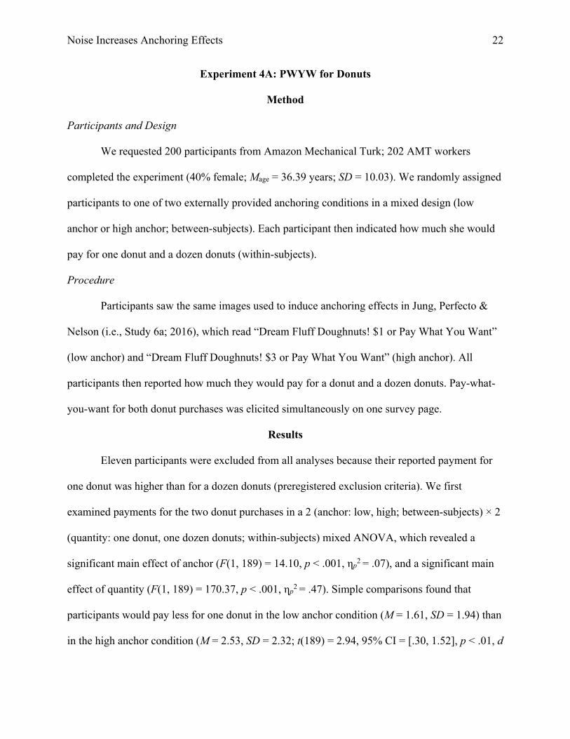
Experiment 4A: PWYW for Donuts

Method



completed the experiment (40% female; Mage = 36.39 years; SD = 10.03). We randomly assigned

participants to one of two externally provided anchoring conditions in a mixed design (low

anchor or high anchor; between-subjects). Each participant then indicated how much she would

pay for one donut and a dozen donuts (within-subjects).

Procedure

Participants saw the same images used to induce anchoring effects in Jung, Perfecto &

Nelson (i.e., Study 6a; 2016), which read “Dream Fluff Doughnuts! $1 or Pay What You Want”

(low anchor) and “Dream Fluff Doughnuts! $3 or Pay What You Want” (high anchor). All

participants then reported how much they would pay for a donut and a dozen donuts. Pay-what-

you-want for both donut purchases was elicited simultaneously on one survey page.

Results

Eleven participants were excluded from all analyses because their reported payment for

one donut was higher than for a dozen donuts (preregistered exclusion criteria). We first

examined payments for the two donut purchases in a 2 (anchor: low, high; between-subjects) × 2

(quantity: one donut, one dozen donuts; within-subjects) mixed ANOVA, which revealed a

significant main effect of anchor (F(1, 189) = 14.10, p < .001, ηp2 = .07), and a significant main

effect of quantity (F(1, 189) = 170.37, p < .001, ηp2 = .47). Simple comparisons found that

participants would pay less for one donut in the low anchor condition (M = 1.61, SD = 1.94) than

in the high anchor condition (M = 2.53, SD = 2.32; t(189) = 2.94, 95% CI = [.30, 1.52], p < .01, d


23

= .43), and would pay less for one dozen donuts in the low anchor condition (M = 8.67, SD =

8.75) than in the high anchor condition (M = 14.35, SD = 12.60; t(189) = 3.60, 95% CI = [2.56,

8.79], p < .001, d = .52). A significant anchor × quantity interaction (F(1, 189) = 10.843, p

= .001, ηp2 = .05), however, showed that the anchoring effect was larger for a dozen donuts than

for a single donut (Figure 3).

Experiment 4B: WTA for Unpleasant Tones

Method



completed the experiment (42% female; Mage = 37.80 years; SD = 10.87). We randomly assigned

participants to one of two anchoring conditions in a mixed design (no, or low anchor; between-

subjects). Each participant reported her willingness-to-accept (WTA) for listening to an

unpleasant tone for 60 seconds, 180 seconds, and 300 seconds (within-subjects).

Procedure

In the no anchor condition, participants saw no anchor. We first asked participants to put

on their headphones (if they used them) and adjust their device volume (e.g., computer,

smartphone) to a comfortable level. Participants then listened to a 30-second sample of an

unpleasant tone, the same tone used in Maniadis, Tufano & List (2014). Next, they reported the

minimum amount of money they would be willing to accept to listen to the same tone for 60

seconds, 180 seconds, and 300 seconds. Participants reported values for all three durations

simultaneously on one survey page.

In the low anchor condition, we asked participants, “Would you be willing to repeat the

same experience for $0.10? (Yes/No)” immediately after they listened to the tone sample for 30


24

seconds. They then reported their minimum amount of money for which they would be willing to

listen to the same tone for 60 seconds, 180 seconds, and 300 seconds, just as controls. Finally, all

participants responded to a manipulation check verifying that they listened to the sample tone

[i.e., “To which of the below was the sound most similar? (Police siren/Truck horn/Vacuum

cleaner/High pitched beep)”].

Results

Fifty participants were excluded from all analyses because they failed to correctly

identify the tone as a “high pitched beep” (preregistered exclusion criteria). We first examined

WTA for the three durations in a 2 (anchor: no, low; between-subjects) × 3 (duration: 60

seconds, 180 seconds, 300 seconds; within-subjects) mixed ANOVA, which revealed a

significant main effect of anchor (F(1, 145) = 7.74, p < .01, ηp2 = .05), and a significant main

effect of duration (F(1, 145) = 137.83, p < .001, ηp2 = .49). More important, these main effects

were qualified by a significant anchor × duration interaction (F(1, 145) = 10.55, p = .001, ηp2

= .07), suggesting that the anchoring effect increased with the duration of unpleasant tone.

Simple comparisons showed that participants were willing to accept less to listen to the tone for

300 seconds in the low anchor condition (M = $3.68, SD = 3.27) than in the no anchor condition

(M = $5.84, SD = 3.76; t(145) = 3.72, 95% CI = [1.01, 3.31], p < .001, d = .61). Similarly,

participants were willing to accept less to listen to the tone sample for 180 seconds in the low

anchor condition (M = $2.46, SD = 2.87) than in the no anchor condition (M = $3.51, SD = 2.80;

t(145) = 2.26, 95% CI = [.13, 1.98], p < .05, d = .37). However, participants were not willing to

accept less to listen to the tone for 60 seconds in the low anchor condition (M = $2.04, SD =

2.62) than in the no anchor condition (M = $1.51, SD = 2.54; t(145) = 1.25, 95% CI = [-.31,

1.37], p = .22, d = .21; see Figure 3).


25

Figure 3. Pay-what-you-want for donuts in Experiment 4A (left panel) and willingness-to-accept to listen to an unpleasant tone in

Experiment 4B (right panel), by anchor and stimulus magnitude. Error bars ±1 SEM.


26

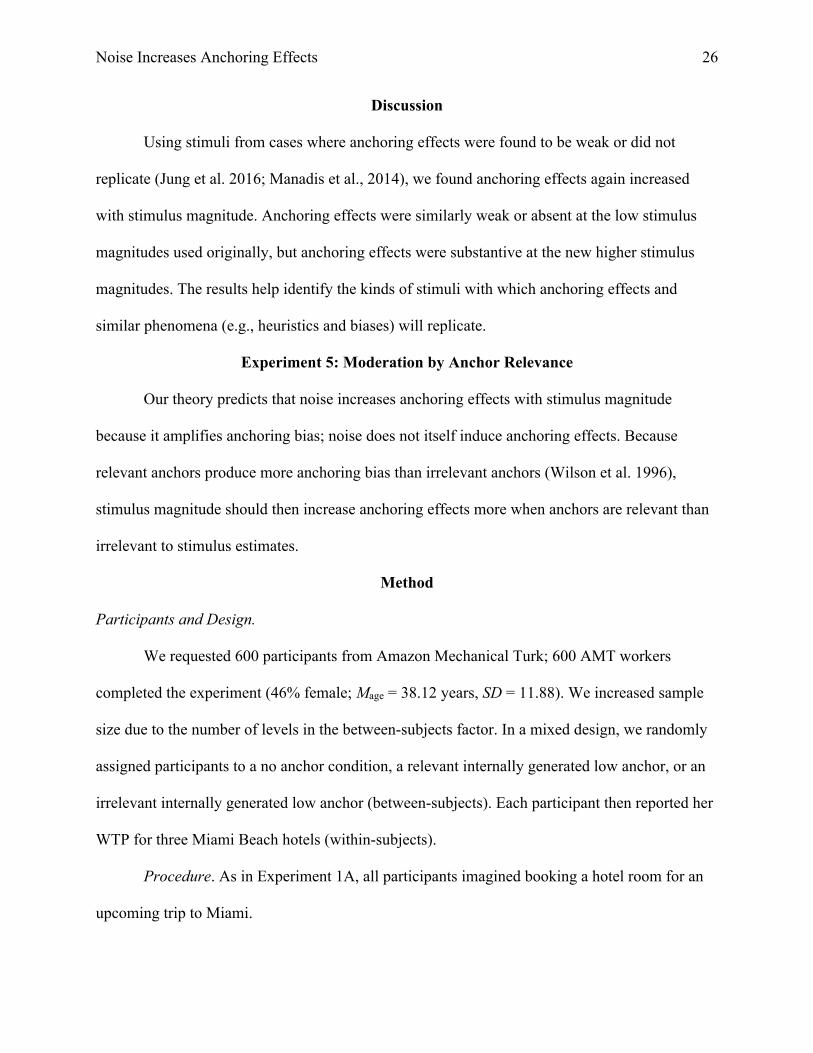
Discussion

Using stimuli from cases where anchoring effects were found to be weak or did not

replicate (Jung et al. 2016; Manadis et al., 2014), we found anchoring effects again increased

with stimulus magnitude. Anchoring effects were similarly weak or absent at the low stimulus

magnitudes used originally, but anchoring effects were substantive at the new higher stimulus

magnitudes. The results help identify the kinds of stimuli with which anchoring effects and

similar phenomena (e.g., heuristics and biases) will replicate.

Experiment 5: Moderation by Anchor Relevance

Our theory predicts that noise increases anchoring effects with stimulus magnitude

because it amplifies anchoring bias; noise does not itself induce anchoring effects. Because

relevant anchors produce more anchoring bias than irrelevant anchors (Wilson et al. 1996),

stimulus magnitude should then increase anchoring effects more when anchors are relevant than

irrelevant to stimulus estimates.

Method

Participants and Design.


completed the experiment (46% female; Mage = 38.12 years, SD = 11.88). We increased sample

size due to the number of levels in the between-subjects factor. In a mixed design, we randomly

assigned participants to a no anchor condition, a relevant internally generated low anchor, or an

irrelevant internally generated low anchor (between-subjects). Each participant then reported her

WTP for three Miami Beach hotels (within-subjects).

Procedure. As in Experiment 1A, all participants imagined booking a hotel room for an

upcoming trip to Miami.


27

In the hotel anchor condition, participants first saw a picture, the name and rating for a 1-

star anchor Miami Beach hotel and reported their WTP (per night) for it. On a subsequent page,

they saw a picture, the name and rating for each of three target Miami Beach hotels (2-star, 3-

star, and 4-star), as in Experiments 1A, and reported their WTP (per night) for one room in each

hotel.

In the no anchor condition, participants first reported their WTP (per night) for the three

target hotels, and then saw and reported their WTP (per night) for the 1-star anchor hotel.

In the jeans anchor condition, participants first saw the brand logo of Levis and stated

their WTP for one pair of Levis jeans. They then saw the same information about each of the

three target hotels and reported their WTP (per night) for one room in each hotel.

In all conditions, participants reported their WTP ($USD) for each stimulus in a unique

open response box.

Results

Anchor. Examining WTP for the anchor itself across conditions with ANOVA revealed a

marginal main effect of condition (F(2, 597) = 2.79, p = .06). Post hoc analyses revealed no

significant difference in WTP for the anchor between the no anchor condition (M = $66.91, SD =

55.62) and the hotel anchor condition (M = $60.63, SD = 58.38; p = .30). WTP for the anchor in

the jeans anchor condition (M = $52.44, SD = 68.74) was significantly lower than WTP for

anchor in the no anchor condition (p = .02). Most important, WTP for the anchor in the jeans

anchor condition did not differ significantly from WTP for the anchor in the hotel anchor

condition (t(198) = 21.88, p < .18).

Targets. We examined the moderating effect of anchor relevance on WTP for the target

hotels in a 3 (anchor: no, hotel, jeans; between-subjects) × 3 (hotel: 2-star, 3-star, 4-star; within-


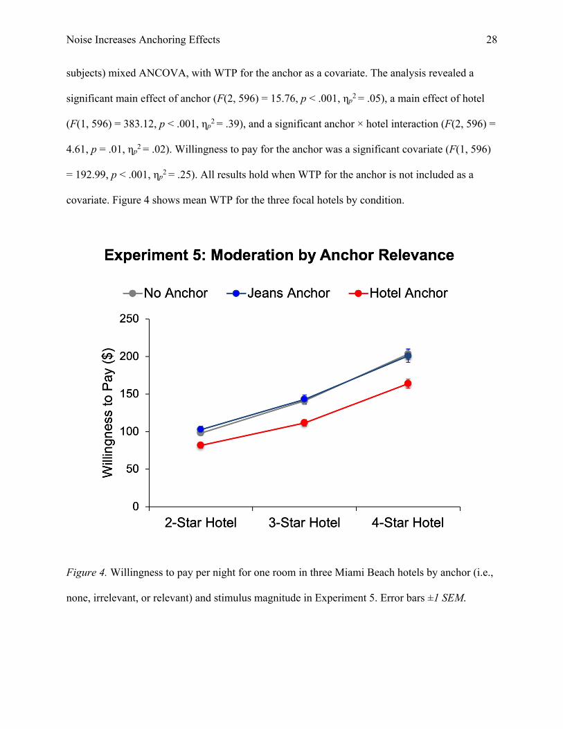
28

subjects) mixed ANCOVA, with WTP for the anchor as a covariate. The analysis revealed a

significant main effect of anchor (F(2, 596) = 15.76, p < .001, ηp2 = .05), a main effect of hotel

(F(1, 596) = 383.12, p < .001, ηp2 = .39), and a significant anchor × hotel interaction (F(2, 596) =

4.61, p = .01, ηp2 = .02). Willingness to pay for the anchor was a significant covariate (F(1, 596)

= 192.99, p < .001, ηp2 = .25). All results hold when WTP for the anchor is not included as a

covariate. Figure 4 shows mean WTP for the three focal hotels by condition.

Figure 4. Willingness to pay per night for one room in three Miami Beach hotels by anchor (i.e.,

none, irrelevant, or relevant) and stimulus magnitude in Experiment 5. Error bars ±1 SEM.


29

We next decomposed this interaction in pairwise comparisons of conditions using

separate 2 × 3 mixed ANCOVAs. Comparing the no anchor and the hotel anchor conditions

revealed a significant 2 (anchor: no, hotel) × 3 (hotel: 2-star, 3-star, 4-star) interaction (F(1, 398)

= 9.27, p = .002, ηp2 = .02). Simple comparisons showed that participants were willing to pay

significantly less for the 4-star hotel in the hotel anchor condition (M = $163.85, SD = 84.98)

than in the no anchor condition (M = $203.29, SD = 105.09; t(399) = 4.14, 95% CI = [20.71,

58.17], p < .001, d = .41). They were also willing to pay less for the 3-star and 2-star hotel in the

hotel anchor condition than in the no anchor condition (M3-star, no anchor = $141.00, SD = 66.57;

M3-star, hotel anchor = $111.67, SD = 60.45; t(399) = 4.62, 95% CI = [16.86, 41.81], p < .001, d

= .46; M2-star, no anchor = $98.04, SD = 47.61; M2-star, hotel anchor = $81.83, SD = 53.27; t(399) = 3.21,

95% CI = [6.28, 26.14], p = .001, d = .32). Moreover, a 2 (anchor: no, low) × 2 (hotel: 2-star, 4-

star) interaction revealed that this difference between conditions was significantly greater for the

4-star than the 2-star hotel (F(1, 398) = 10.13, p = .002, ηp2 = .03).

Comparing the no anchor and the jeans anchor conditions in a 2 (anchor: no, jeans) × 3

(hotel: 2-star, 3-star, 4-star) ANCOVA found no interaction, (F(1, 393) = .14, p = .71, ηp2

< .001), suggesting that considering an irrelevant anchor did not increase anchoring effects with

stimulus magnitude (M2-star, jeans anchor = $102.71, SD = 66.19; M3-star, jeans anchor = $142.96, SD =

83.93; M4-star, jeans anchor = $200.84, SD =121.08).

Finally, comparing the hotel anchor and the jeans anchor conditions in a 2 (anchor: hotel,

jeans) × 3 (hotel: 2-star, 3-star, 4-star) ANCOVA revealed a significant interaction (F(1, 400) =

4.83, p = .029, ηp2 = .01). Simple comparisons revealed that the WTP for the 4-star hotel was

significantly lower in the hotel anchor condition than in the jeans anchor condition (t(401) =

3.56, 95% CI = [16.54, 57.43], p < .001, d = .35). Differences in WTP for the 3-star and 2-star


30

hotels were also significant between the two anchor conditions (both ts(401) > 4.30, ps ≤ .001).

A 2 (anchor: hotel, jeans) × 2 (hotel: 2-star, 4-star) interaction suggested that this difference

between conditions was significantly greater for the 4-star than the 2-star hotel (F(1, 400) = 5.09,

p = .025, ηp2 = .01).

Discussion

Noise alone did not increase anchoring effects. Anchoring effects increased with stimulus

magnitude only when the anchor was relevant to targets––when there was an anchoring bias to

amplify.

Experiments 6A and 6B: Anchoring Effects, Anchoring Bias, and Noise

In Experiments 6A and 6B, we directly compared effects of stimulus magnitude on

anchoring effects, anchoring bias, and noise. We elicited range and point estimates for small and

large magnitude stimuli in low and high external anchor conditions. We calculated range widths

and anchoring effects, as before, but also calculated anchoring bias with a skew index (Epley &

Gilovich, 2006). We predicted stimulus magnitude would increase range widths and anchoring

effects, even though anchoring bias would be similar for both small and large magnitude stimuli.


Method



completed Experiment 6A (49% female; Mage = 38.51 years; SD = 12.20). The design was

adapted from Experiment 3A. We randomly assigned participants to a low or high external

anchor condition (between-subjects). Participants then made a range or point estimate involving


31

WTP for a standard room (per night) in either a 2-star or a 4-star Miami Beach hotel (all

between-subjects).

Procedure

All participants imagined vacationing after the pandemic concluded in Miami in January

2023. Participants randomly assigned to the low (external) anchor condition saw the 1-star

Miami Beach hotel and its $44 rate, as in Experiment 3A. Participants randomly assigned to the

high (external) anchor condition saw the 5-star Miami Beach hotel and its $610 rate, as in

Experiment 3A. On the same page, participants also saw one target hotel: either the 2-star or the

4-star Miami Beach hotel from Experiment 3A (i.e., with no rate displayed). On a separate page,

participants randomly assigned to a point estimate condition then reported their maximum WTP

for a room ($USD per night) in that target hotel in an open response box. Participants randomly

assigned to a range estimate condition estimated the maximum and minimum possible average

WTP of the 100 participants who made a point estimate for the target hotel. We had these

participants estimate averages because the minimum and maximum possible estimates could

range from zero to infinity. Range estimates were reported in two separate open-ended response

boxes.

Results

All means and confidence intervals are reported in Table 2.

Point Estimates (Anchoring Effects)

We examined point estimates in a 2 (anchor: low, high) × 2 (hotel: 2-star, 4-star)

between-subjects ANOVA. It revealed significant main effects of anchor (F(1, 200) =98.04, p

< .001, ηp2 = .33) and hotel (F(1, 200) = 104.72, p < .001, ηp2 = .34). More important, these main

effects were qualified by a significant anchor × hotel interaction (F(1, 200) = 5.39, p = .02, ηp2


32

= .03). Participants were willing to pay less for the 4-star hotel in the low anchor condition than

in the high anchor condition (t(100) = 6.86, 95% CI = [114.80, 208.16], p < .001, d = 1.38).

Participants were also willing to pay less for the 2-star hotel in the low anchor condition than in

the high anchor condition (t(100) = 8.33, 95% CI = [76.29, 123.99], p < .001, d = 1.45). The

significant interaction revealed that this difference in point estimates between anchor conditions

was significantly greater for the 4-star than the 2-star hotel.

Range Estimates (Noise)

We converted range estimates to widths (i.e., maximum – minimum) and compared them

in a 2 (anchor: low, high) × 2 (hotel: 2-star, 4-star) between-subjects ANOVA. It revealed the

predicted significant effect of hotel, such that ranges were wider for the 4-star than 2-star hotel

(F(1, 199) = 44.29, p < .001, ηp2 = .18). Exploratory analyses revealed that there was also a

significant main effect of anchor (F(1, 199) = 6.67, p = .01, ηp2 = .03), such that ranges were

wider in high than low anchor conditions, and a significant anchor × hotel interaction (F(1, 199)

= 5.02, p = .03, ηp2 = .03). Range estimates were still significantly wider for the 4-star than the 2-

star hotel in the low anchor condition (M4-star = 182.89, SD = 180.69; M2-star = 41.43, SD = 34.76;

t(100) = 5.74, p < .001, 95% CI = [92.54, 190.39], d = 1.09) and in the high anchor condition

(M4-star = 188.33, SD = 107.38; M2-star = 118.11, SD = 88.84; t(99) = 3.51, p = .001 95% CI =

[30.50, 109.94], d = .71). We interpret these wider ranges with higher than lower anchors as

further evidence of the influence of scalar variability. In other words, the larger anchor may have

made the value of the hotels appear greater and thus increased the noise in their estimation, but

this interpretation is admittedly speculative.


33

Skew Index (Anchoring Bias)

We then calculated a skew index (Epley & Gilovich, 2006) to quantify anchoring bias

across point estimate conditions. We divided (a) the difference between each participant’s point

estimate and the range endpoint nearest to the anchor by (b) the total range width of plausible

values [(point estimate – the maximum or minimum plausible value)/(the maximum plausible

value – the minimum plausible value)]. The range estimate values used for each participant were

specific to their treatment (e.g., low anchor, 2-star hotel). We then multiplied the skewness index

in the high anchor conditions by -1 so adjustment could be directly compared to the low anchor

conditions. Generally, a lower skew index suggests greater anchoring bias. Perfectly centered

estimates received a score of .50. Estimates closer to the anchor, cases of insufficient correction

from the anchor, scored less than .50. Estimates beyond the midpoint, cases of overcorrection

from the anchor, scored higher than .50

We examined skew indices in a 2 (anchor: low, high) × 2 (hotel: 2-star, 4-star) between-

subjects ANOVA. It revealed no significant main effect of anchor (F(1, 200) = 1.55, p = .22, ηp2

< .01), no main effect of hotel (F(1, 200) = .83, p = .36, ηp2 < .01), and no anchor × hotel

interaction (F(1, 200) = .15, p = .70, ηp2 < .01).


34

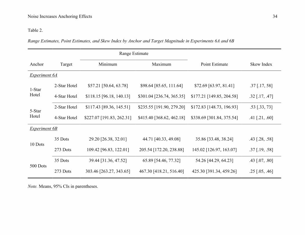
Table 2.

Range Estimates, Point Estimates, and Skew Index by Anchor and Target Magnitude in Experiments 6A and 6B

Range Estimate

Anchor Target Minimum Maximum Point Estimate Skew Index

Experiment 6A

1-Star Hotel

2-Star Hotel $57.21 [50.64, 63.78] $98.64 [85.65, 111.64] $72.69 [63.97, 81.41] .37 [.17, 58]

4-Star Hotel $118.15 [96.18, 140.13] $301.04 [236.74, 365.35] $177.21 [149.85, 204.58] .32 [.17, .47]

5-Star Hotel

2-Star Hotel $117.43 [89.36, 145.51] $235.55 [191.90, 279.20] $172.83 [148.73, 196.93] .53 [.33, 73]

4-Star Hotel $227.07 [191.83, 262.31] $415.40 [368.62, 462.18] $338.69 [301.84, 375.54] .41 [.21, .60]

Experiment 6B

10 Dots 35 Dots 29.20 [26.38, 32.01] 44.71 [40.33, 49.08] 35.86 [33.48, 38.24] .43 [.28, .58]

273 Dots 109.42 [96.83, 122.01] 205.54 [172.20, 238.88] 145.02 [126.97, 163.07] .37 [.19, .58]

500 Dots 35 Dots 39.44 [31.36, 47.52] 65.89 [54.46, 77.32] 54.26 [44.29, 64.23] .43 [.07, .80]

273 Dots 303.46 [263.27, 343.65] 467.30 [418.21, 516.40] 425.30 [391.34, 459.26] .25 [.05, .46]

Note. Means, 95% CIs in parentheses.


35

Experiment 6B: Counts in Dot Arrays

Method



completed Experiment 6B (46% female; Mage = 39.59 years; SD = 12.42). The paradigm was the

same as in Experiment 6A, with the dot arrays used in Experiment 3B as anchors and targets. We

randomly assigned participants to a low or high external anchor condition (between-subjects).

Participants then made a range or point estimate for a 35-dot or 273-dot array (all between-

subjects).

Procedure

As in Experiment 3B, participants randomly assigned to the low (external) anchor

condition saw a 10-dot array. Participants randomly assigned to the high (external) anchor

condition saw a 500-dot array. Participants were told the number of dots in that array (i.e., 10 or

500), and that all dots were the same size in the experiment. Next, participants were randomly

assigned to see a 35-dot or a 273-dot array (the number of dots was not labeled). Participants

randomly assigned to a point estimate condition estimated the number of dots in the array an

open response box. Participants randomly assigned to a range estimate condition estimated the

maximum and minimum plausible number of dots in the array. Range estimates were reported in

two separate open-ended response boxes.

Results

All means and confidence intervals are reported in Table 2.

Point Estimates (Anchoring Effects)


36

We examined point estimates in a 2 (anchor: low, high) × 2 (dot array: 35, 273) between-

subjects ANOVA. It revealed significant main effects of anchor (F(1, 196) = 241.14, p < .001,

ηp2 = .55), dot array (F(1, 196) = 623.284, p < .001, ηp2

= .76), and the predicted significant

anchor × dot array interaction (F(1, 196) = 185.37, p < .001, ηp2 = .49). Participants estimated a

significantly lower count for the 273-dot array in the low anchor condition than in the high

anchor condition (t(99) = 15.19, 95% CI = [243.67, 316.89], p < .001, d = 2.98). Participants also

estimated a significantly lower count for the 35-dot array in the low anchor condition than in the

high anchor condition (t(97) = 4.14, 95% CI = [9.57, 27.24], p < .001, d = .78). The significant

interaction revealed that the anchoring effect on point estimates was larger for the 273-dot array

than the 35-dot array.

Range Estimates (Noise)

We converted range estimates to widths (i.e., maximum – minimum) and compared them

in a 2 (anchor: low, high) × 2 (dot array: 35, 273) between-subjects ANOVA. Most important, it

revealed the predicted significant effect of dot array (F(1, 196) = 108.82, p < .001, ηp2 = .37).

Exploratory analyses revealed there was also a significant main effect of anchor (F(1, 196) =

14.17, p < .001, ηp2 = .07), such that ranges were wider in the high than low anchor conditions,

and a significant anchor × dot array interaction (F(1, 196) = 7.39, p < .01, ηp2 = .04). Range

estimates were still significantly wider for the 273-dot array than the 35-dot array in the low

anchor condition (M273-dot array = 96.12, SD = 84.25; M35-dot array = 15.51, SD = 14.59; t(89) = 5.84,

p < .001, 95% CI = [53.20, 108.02], d = 1.29) and in the high anchor condition (M273-dot array =

163.85, SD = 115.73; M35-dot array = 26.44, SD = 31.05; t(107) = 9.00, p < .001, 95% CI = [107.15,

167.65], d = 1.62). As for Experiment 6A, we interpret the wider ranges with higher than lower

anchors as further evidence of the influence of scalar variability. The larger anchor may have


37

made the arrays appear larger in number and thus increased the noise in their estimation, but

again this interpretation is admittedly speculative.

Skew Index (Anchoring Bias)

Skew index was calculated using the same method as Experiment 6A. We examined

skew index in a 2 (anchor: low, high) × 2 (dot array: 35, 273) between-subjects ANOVA, which

revealed no significant main effect of anchor (F(1, 196) = .24, p = .62, ηp2 < .01), no main effect

of dot array (F(1, 196) = 1.11, p = .29, ηp2 < .01), and no anchor × dot array interaction (F(1,

196) = .30, p = .59, ηp2 < .01).

Discussion

Anchoring effects on point estimates and ranges of plausible values increased with

stimulus magnitude. Anchoring bias as measured by the skew index, however, was not

statistically different for the small and large magnitude hotels or dot arrays (Fs ≦ 1.11, ps

≧ .292). Anchoring effects appear to have increased with stimulus magnitude due to increased

noise in stimulus representations, not due to increased anchoring bias.

General Discussion

Anchoring effects increased with stimulus magnitude. This appears to have been due to

an increase in judgmental noise. Ranges of plausible values for point estimates increased with

stimulus magnitudes, but anchoring bias did not. As scalar variability would predict, regressing

standard deviations on means of all target estimates also revealed a positive linear relationship

between the noise and magnitude of point estimates (β1 = .44, SE = .02; t(60) = 19.96, p < .001;

F(1, 60) = 398.32, p < .001, R2 = .87; Figure 5).


38

Figure 5. Standard deviation of point estimates by mean of point estimates for all targets.

Alternative explanations, such as a floor effect of scales or an inability to differentiate

low anchors from low magnitude stimuli are not supported by the data. The lower bound of

plausible ranges for all low magnitude stimuli (i.e., average minimum) was significantly greater

than zero (all ts ≧ 3.37, all ps ≦ .001) and significantly greater than all low anchors (all ts ≧ 2.53,

all ps ≦ .015). Anchoring bias induced by low and high anchors did not differ for the 2-star hotel

in Experiment 6A or the small dot array in Experiment 6B (ts < 1, p’s ≧ .283). An ancillary

experiment found the effect of stimulus magnitude on anchoring effects holds when stimulus

values are negative integers (see SOM), and comparisons between no anchor and high anchors


39

conditions in Experiments 1 and 2B (see also Experiment 3C in SOM), where censoring effects

should not apply, also found an increase in anchoring effects with stimulus magnitude.

Our findings elucidate the roles of noise and bias in anchoring effects. Noise modulates

the size of anchoring effects by modulating anchoring bias. Our findings and framework

contribute to the anchoring literature by reconciling questions regarding the replicability and

prevalence of anchoring effects (Jung et al., 2016; Maniadas et al., 2014). The stimuli used in

that research were so low in magnitude that they induced insufficient noise to observe sizeable

anchor effects. More important, our findings suggest a reexamination of how anchoring effects

are moderated by factors such as cognitive load, intoxication, subjective confidence, knowledge,

and incentives (Epley & Gilovich, 2006; Jacowitz & Kahneman, 1995; Mussweiler & Strack,

2000; Simmons et al., 2010; Smith et al., 2013). It is often assumed they modulate anchoring

effects by influencing anchoring bias, but these factors could also modulate anchoring effects by

influencing judgmental noise. Cognitive load or intoxication, for instance, may increase

anchoring effects in point estimates by reducing adjustment from an anchor (i.e., anchoring bias)

or by widening the range of values perceived to be plausible (i.e., noise). More broadly, our

framework shows how noise can modulate effects of heuristics and biases on judgments under

uncertainty, and it provides a paradigm for testing the role of noise in these phenomena.


40

References

Chapman, G. B., & Johnson, E. J. (1994). The limits of anchoring. Journal of Behavioral

Decision Making, 7(4), 223–242.

Englich, B., Mussweiler, T., & Strack, F. (2006). Playing dice with criminal sentences: The

influence of irrelevant anchors on experts’ judicial decision making. Personality and Social

Psychology Bulletin, 32(2), 188–200.

Epley, N., & Gilovich, T. (2006). The anchoring-and-adjustment heuristic: Why the adjustments

are insufficient. Psychological Science, 17(4), 311–318.

Feigenson, L., Dehaene, S., & Spelke, E. (2004). Core systems of number. Trends in Cognitive

Sciences, 8(7), 307–314.

Jacowitz, K. E., & Kahneman, D. (1995). Measures of anchoring in estimation tasks. Personality

and Social Psychology Bulletin, 21(11), 1161–1166.

Jung, M. H., Perfecto, H., & Nelson, L. D. (2016). Anchoring in payment: Evaluating a

judgmental heuristic in field experimental settings. Journal of Marketing Research, 53(3),

354–368.

Kahneman, D., Rosenfield, A. M., Gandhi, L., & Blaser, T. (2016). Noise: How to overcome the

high, hidden cost of inconsistent decision making. Harvard Business Review, 94(10), 38–

46.

Maniadis, Z., Tufano, F., & List, J. A. (2014). One swallow doesn’t make a summer: New

evidence on anchoring effects. American Economic Review, 104(1), 277–290.

Mussweiler, T., & Strack, F. (2000). Numeric judgments under uncertainty: The role of

knowledge in anchoring. Journal of Experimental Social Psychology, 36(5), 495-518.

Northcraft, G. B., & Neale, M. A. (1987). Experts, amateurs, and real estate: An anchoring-and-


41

adjustment perspective on property pricing decisions. Organizational Behavior and Human

Decision Processes, 39(1), 84–97.

Quattrone, G. A., Lawrence, C. P., Finkel, S. E., & Andrus, D. C. (1984). Explorations in

anchoring: The effects of prior range, anchor extremity, and suggestive hints. Unpublished

Manuscript.

Simmons, J. P., LeBoeuf, R. A., & Nelson, L. D. (2010). The effect of accuracy motivation on

anchoring and adjustment: Do people adjust from provided anchors? Journal of Personality

and Social Psychology, 99(6), 917–932.

Smith, A. R., Windschitl, P. D., & Bruchmann, K. (2013). Knowledge matters: Anchoring

effects are moderated by knowledge level. European Journal of Social Psychology, 43(1),

97–108.

Tversky, A., & Kahneman, D. (1974). Judgment under uncertainty: Heuristics and biases.

Science, 185(4157), 1124–1131.

Wilson, T. D., Houston, C. E., Etling, K. M., & Brekke, N. (1996). A new look at anchoring

effects: Basic anchoring and its antecedents. Journal of Experimental Psychology: General,

125(4), 387–402.


42

Acknowledgements

We sincerely thank Gretchen Chapman, Fiery Cushman, Nicholas Epley, Daniel

Kahneman, Thomas Mussweiler, and Lawrence Williams for helpful comments about this work.


SUPPLEMENTAL ONLINE MATERIAL

I. Preregistrations

Experiment 1A: https://aspredicted.org/blind.php?x=6ec32n

Experiment 1B: https://aspredicted.org/blind.php?x=p6hj24

Experiment 2A: https://aspredicted.org/blind.php?x=q6hs5c

Experiment 2B: https://aspredicted.org/blind.php?x=dw6ap9

Experiment 3A: https://aspredicted.org/blind.php?x=hr6me8

Experiment 3B: https://aspredicted.org/blind.php?x=bx9ya3

Experiment 4A: https://aspredicted.org/blind.php?x=nb2eh8

Experiment 4B: https://aspredicted.org/blind.php?x=tb38ed

Experiment 5: https://aspredicted.org/blind.php?x=4fk93p

Experiment 6A: https://aspredicted.org/blind.php?x=in2x82

Experiment 6B: https://aspredicted.org/blind.php?x=zm5yd3


II. Target Stimuli in Experiments 1A-3B

Figure A1: Miami Hotels

2 STAR HOTEL 3 STAR HOTEL 4 STAR HOTEL

Hampton Inn Miami South Beach

Cadillac Hotel & Beach Club

The Palms Hotel

Maximum Willingness-to-Pay ($)


Figure A2: Dog Breeds

Bernese Mountain Dog

American Staffordshire Terrier

Basenji

Estimated Weight (lbs.)


Figure A3: Servings of McDonald’s French Fries

Small Fries Medium Fries Large Fries

Estimated Calories


Figure A4: Dot Arrays

Graph A Graph B Graph C

Estimated Number of Dots


III. Pretests: Extended Results

Miami Hotels. As predicted, the range of plausible prices of the 4-star hotel was

significantly wider (Mmin = $200.24, SD = 173.83; Mmax = $344.46, SD = 187.74) than the range

of plausible prices of the 3-star hotel (Mmin = $143.14, SD = 110.37; Mmax = $259.08, SD =

164.55; t(49) = 2.16, 95% CI = [1.99, 54.57], p = .036, d = .31) and the 2-star hotel (Mmin =

$103.88, SD = 87.15; Mmax = $193.14, SD = 169.20; t(49) = 2.88, 95% CI = [16.65, 93.27], p

= .006, d = .41). The range of plausible prices of the 3-star hotel was also significantly wider

than that of the 2-star hotel (t(49) = 2.75, 95% CI = [7.20, 46.16], p = .008, d = .39).

Dog Breeds. The range of plausible weights of Bernese Mountain Dogs was significantly

wider (Mmin = 70.60, SD = 43.78; Mmax = 145.35, SD = 63.85) than the range of the plausible

weights of American Staffordshire Terriers (Mmin = 45.54, SD = 31.17; Mmax = 99.31, SD = 57.10;

t(47) = 3.58, 95% CI = [9.19, 32.77], p = .001, d = .52) and Basenjis (Mmin = 22.92, SD = 20.36;

Mmax = 52.31, SD = 26.25; t(47) = 7.25, 95% CI = [32.76, 57.95], p < .001, d = 1.05). The range

of the plausible weights of American Staffordshire Terriers was also significantly wider than that

of Basenjis (t(47) = 4.49, 95% CI = [13.46, 35.29], p < .001, d = .65).

French Fries. The range of plausible calories of the large serving of McDonald’s French

Fries was significantly wider (Mmin = 266.98, SD = 264.12; Mmax = 423.37, SD = 464.84) than

that of the medium serving of McDonald’s French Fries (Mmin = 203.23, SD = 205.99; Mmax =

320.23, SD = 337.84; t(51) = 2.38, 95% CI = [6.13, 72.64], p = .021, d = .33) and the small

serving of McDonald’s French Fries (Mmin = 141.48, SD = 153.53; Mmax = 223.46, SD = 236.45;

t(51) = 3.36, 95% CI = [29.97, 118.84], p = .001, d = .47). The range of plausible calories of the

medium serving of McDonald’s French Fries was also significantly wider than that of the small

serving of McDonald’s French Fries (t(51) = 3.01, 95% CI = [11.69, 58.35], p = .004, d = .42).


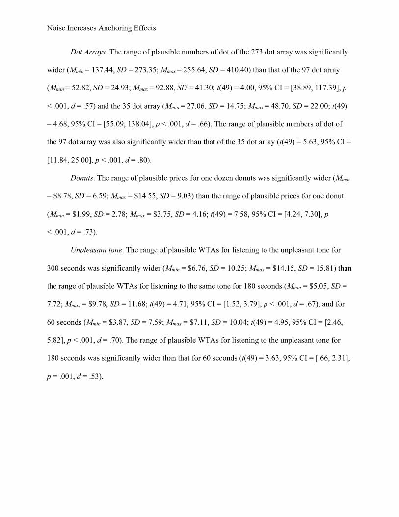
Dot Arrays. The range of plausible numbers of dot of the 273 dot array was significantly

wider (Mmin = 137.44, SD = 273.35; Mmax = 255.64, SD = 410.40) than that of the 97 dot array

(Mmin = 52.82, SD = 24.93; Mmax = 92.88, SD = 41.30; t(49) = 4.00, 95% CI = [38.89, 117.39], p

< .001, d = .57) and the 35 dot array (Mmin = 27.06, SD = 14.75; Mmax = 48.70, SD = 22.00; t(49)

= 4.68, 95% CI = [55.09, 138.04], p < .001, d = .66). The range of plausible numbers of dot of

the 97 dot array was also significantly wider than that of the 35 dot array (t(49) = 5.63, 95% CI =

[11.84, 25.00], p < .001, d = .80).

Donuts. The range of plausible prices for one dozen donuts was significantly wider (Mmin

= $8.78, SD = 6.59; Mmax = $14.55, SD = 9.03) than the range of plausible prices for one donut

(Mmin = $1.99, SD = 2.78; Mmax = $3.75, SD = 4.16; t(49) = 7.58, 95% CI = [4.24, 7.30], p

< .001, d = .73).

Unpleasant tone. The range of plausible WTAs for listening to the unpleasant tone for

300 seconds was significantly wider (Mmin = $6.76, SD = 10.25; Mmax = $14.15, SD = 15.81) than

the range of plausible WTAs for listening to the same tone for 180 seconds (Mmin = $5.05, SD =

7.72; Mmax = $9.78, SD = 11.68; t(49) = 4.71, 95% CI = [1.52, 3.79], p < .001, d = .67), and for

60 seconds (Mmin = $3.87, SD = 7.59; Mmax = $7.11, SD = 10.04; t(49) = 4.95, 95% CI = [2.46,

5.82], p < .001, d = .70). The range of plausible WTAs for listening to the unpleasant tone for

180 seconds was significantly wider than that for 60 seconds (t(49) = 3.63, 95% CI = [.66, 2.31],

p = .001, d = .53).


Table A1.

Mean Point Estimates by Anchor and Stimulus Magnitude in Experiments 1A-3B.

Stimulus

Magnitude

Anchor

Experiment None Low High

1A. Miami Hotels (WTP)

2-Star 109.43 (93.13) 79.72 (80.53) 142.85 (110.22)

3-Star 145.08 (76.37) 107.81 (75.62) 209.23 (117.69)

4-Star 197.28 (100.42) 146.61 (81.10) 330.10 (176.07)

1B. Dog Breeds (Pounds)

Basenji 32.38 (15.45) 49.51 (25.19)

AST 59.80 (25.52) 90.73 (34.75)

BMD 90.67 (36.00) 142.85 (35.51)

2A. French Fries (Cal)

Small 226.27 (127.23) 231.98 (116.12)

Medium 384.38 (192.85) 351.22 (163.46)

Large 563.05 (258.35) 493.68 (219.88)

2B. Dot Arrays (Counts)

35-Dot 40.18 (18.48) 40.42 (20.80)

97-Dot 84.72 (50.89) 91.17 (50.23)

273-Dot 185.39 (150.73) 244.61 (178.35)

3A. Miami Hotels (WTP)

2-Star 75.42 (53.57) 171.25 (105.71)

4-Star 154.04 (119.08) 356.35 (149.41)

3B. Dot Arrays (Counts)

35-Dot 33.41 (6.89) 46.05 (30.10)

273-Dot 153.94 (113.78) 390.15 (147.98)

Note: Standard deviations in parentheses.


IV. Negative Integer Experiment: Freezing Points

Method

Pretest

We recruited 50 participants from Amazon Mechanical Turk, and 50 AMT workers

completed the pretest. Participants were told the alcohol content of beer, wine, and vodka, and

the relationship between alcohol content and freezing temperature. Participants were not shown

pictures of each beverage. In open-ended response boxes, participants estimated the highest

(warmest) and lowest (coldest) temperatures that the freezing point of each beverage might fall

between with 95% confidence.

The range of plausible freezing points of vodka was significantly wider (Mmin = 14.02, SD

= 46.12; Mmax = -39.34, SD = 81.92) than the range of plausible freezing points of wine (Mmin =

29.24, SD = 17.85; Mmax = -15.25, SD = 67.87; t(49) = 2.02, 95% CI = [.03, 17.69], p = .049, d

= .29) and beer (Mmin = 30.32, SD = 16.34; Mmax = -7.74, SD = 63.03; t(49) = 2.94, 95% CI =

[4.85, 25.74], p = .005, d = .42). The range of plausible freezing points of wine was also

significantly wider than the range of plausible freezing points of beer (t(49) = 2.88, 95% CI =

[1.94, 10.93], p = .006, d = .41).

Preregistration

https://aspredicted.org/blind.php?x=az59jw


We recruited 200 participants from Amazon Mechanical Turk. 200 AMT workers

completed Experiment 5 (51% female; Mage = 36.01 years; SD = 11.83). In a mixed design, we


randomly assigned participants to a low or high externally provided anchor (between-subjects).

Each participant then made freezing point estimates for three related stimuli (within-subjects).

Procedure

Participants randomly assigned to a high anchor condition first read that the freezing

point of water is 32°F. In the low anchor condition, participants first read that the freezing point

of ethanol is -173.5°F. In open-ended response boxes appearing on the same page, participants

then estimated the freezing point, in Fahrenheit, of beer, wine, and vodka. The ranking of the

freezing point of the alcoholic beverages was explicit. Participants read the freezing point of

vodka is lower than that of wine, which is lower than that of beer.

Results

Sixty-six participants were excluded from all analyses because they gave freezing point

estimates that were inconsistent with this ranking (i.e., preregistered exclusion criteria). We

examined freezing point estimates of the three target alcohol beverages in a 2 (anchor: low, high;

between-subjects) × 3 (alcohol beverage: beer, wine, vodka; within-subjects) mixed ANOVA. It

revealed a significant main effect of anchor (F(1, 132) = 43.91, p < .001, ηp2 = .25), and a

significant main effect of alcohol beverage (F(1, 132) = 161.40, p < .001, ηp2 = .55). The main

effects were qualified by the predicted significant anchor × alcohol beverage interaction, (F(1,

132) = 19.30, p < .001, ηp2 = .13). As predicted, anchoring effects increased with stimulus

magnitude, even when integers were negative.

Simple comparisons revealed that freezing point estimates for beer were lower when the

anchor was ethanol (M = -15.38, SD = 54.96) than when the anchor was water (M = 20.46, SD =

14.05; t(132) = 5.17, 95% CI = [22.13, 49.55], p < .001, d = .89); freezing point estimates for

wine were lower when the anchor was ethanol (M = -33.87, SD = 60.92) than when the anchor


was water (M = 9.46, SD = 16.80; t(132) = 5.61, 95% CI = [28.06, 58.60], p < .001, d = .97); and

freezing point estimates for vodka were lower when the anchor was ethanol (M = -80.2, SD =

72.67) than when the anchor was water (M = -11.95, SD = 27.72; t(132) = 7.26, 95% CI =

[50.18, 87.77], p < .001, d = 1.26). A significant 2 (anchor: high, low) × 2 (alcohol beverage:

beer, vodka) interaction revealed that anchoring effects were greater for freezing point estimates

for vodka than for beer (F(1, 132) = 21.83, p < .001, ηp2 = .14).


V. Experiment 3C: Counts in Dots Arrays

Method

Preregistration

https://aspredicted.org/blind.php?x=wj23be



completed this experiment (49% female; Mage = 38.28 years; SD = 12.18). We randomly

assigned participants to a high or no externally provided anchor condition (between-subjects),

and to evaluate a 35-dot or 273 dot array (between-subjects).

Procedure

In the no (external) anchor condition, participants saw and estimated the number of dots

in either a 35-dot or 273-dot array. In the high (external) anchor condition, participants were first

presented with a 500-dot array. They were told the number of dots depicted in that anchor array.

Next, they saw and estimated the number of dots in either a 35-dot or 273-dot array. Dot

estimates were made in open-ended response boxes.

Results

We tested our directional predictions, examining dot estimates in a 2 (anchor: no, high) ×

2 (dot array: 35, 273) between-subjects ANOVA. It revealed significant main effects of anchor

(F(1, 401) = 79.27, p < .001, ηp2 = .17) and of array (F(1, 401) = 609.30, p < .001, ηp2 = .60).

More important, there was a significant anchor × array interaction (F(1, 401) = 57.28, p < .001,

ηp2 = .13). The dot estimate for the 273-dot array was significantly lower in the no anchor

condition (M = 213.04, SD = 161.10) than in the high anchor condition (M = 384.05, SD =


128.00; t(199) = 8.25, 95% CI = [130.16, 211.87], p < .001, d = 1.18). Moreover, the dot

estimate for the 35-dot array was significantly lower in the no anchor condition (M = 35.33, SD =

10.18) than in the high anchor condition (M = 19.19, SD = 25.25; t(202) = 4.99, 95% CI = [8.38,

19.34], p < .001, d = .72). However, the significant interaction revealed that this difference

between conditions was significantly larger for the 273-dot array than the 35-dot array.

View publication statsView publication stats

https://www.researchgate.net/publication/351327098

Documents

Noise Increases Anchoring Effects Chang-Yuan Lee and Carey