Embed Size (px)
Citation preview

Noise Simulations of the High-Lift Common Research Model
David P. Lockard,∗ Meelan M. Choudhari,† Veer N. Vatsa† and Matthew D. O’Connell‡
NASA Langley Research Center, Hampton,VA 23681
Benjamin Duda§
Exa GmbH, Landshuter Allee 8, 80637 Munich, Germany
Ehab Fares¶
Exa GmbH, Curiestrasse 4, D-70563, Stuttgart, Germany
The PowerFLOW R© code has been used to perform numerical simulations of the high-lift version of the Com-
mon Research Model (HL-CRM) that will be used for experimental testing of airframe noise. Time-averaged sur-
face pressure results from PowerFLOW R© are found to be in reasonable agreement with those from steady-state
computations using FUN3D. Surface pressure fluctuations are highest around the slat break and nacelle/pylon
region, and synthetic array beamforming results also indicate that this region is the dominant noise source on
the model. The gap between the slat and pylon on the HL-CRM is not realistic for modern aircraft, and most
nacelles include a chine that is absent in the baseline model. To account for those effects, additional simulations
were completed with a chine and with the slat extended into the pylon. The case with the chine was nearly
identical to the baseline, and the slat extension resulted in higher surface pressure fluctuations but slightly re-
duced radiated noise. The full-span slat geometry without the nacelle/pylon was also simulated and found to be
around 10 dB quieter than the baseline over almost the entire frequency range. The current simulations are still
considered preliminary as changes in the radiated acoustics are still being observed with grid refinement, and
additional simulations with finer grids are planned.
Nomenclature
Cp coefficient of pressure
c local deployed chord
p pressure
rms root mean square
VR variable resolution
x, y, z Cartesian coordinates
Superscript:′ perturbation quantity (e.g., p′ = p − po)
Subscript:
o dimensional reference quantity
I. Introduction
Aircraft noise reduction, including that of the airframe, is an important goal of the NASA Advanced Air Transport
Technology (AATT) Project, which is supporting a combined experimental and computational effort to better understand
and mitigate the sources associated with slat noise. The nonpropulsive (or airframe) sources of aircraft noise include
high-lift devices (e.g., the leading-edge slat and trailing-edge flaps) and the aircraft undercarriage. The ranking of these
sources is configuration dependent; however, both model-scale tests1–7 and flyover noise measurements8 have identified
the leading-edge slat as a prominent source of airframe noise during aircraft approach. To further develop airframe
noise reduction technology, NASA is currently planning to construct a 10%-scale version of the High-Lift Common
Research Model (HL-CRM) recently developed by Lacy and Sclafani.9 The original cruise configuration NASA CRM is
an open geometry that has been widely used in the AIAA Drag Prediction Workshops.10 The NASA CRM11 consists of a
contemporary supercritical transonic wing with flow-through nacelles and a fuselage that is representative of a widebody
commercial transport aircraft. The new HL-CRM is also an open geometry that is being used in the AIAA Geometry
and Mesh Generation Workshop12 and 3rd AIAA High-Lift Prediction Workshop.13
∗Aerospace Technologist, Computational AeroSciences Branch, Mail Stop 128, Senior Member, AIAA†Aerospace Technologist, Computational AeroSciences Branch, Mail Stop 128, Associate Fellow, AIAA‡Aerospace Technologist, Computational AeroSciences Branch, Mail Stop 128, Member, AIAA§Senior Application Engineer, Aerospace Applications¶Senior Technical Director, Aerospace Applications; Senior Member AIAA
1 of 18
American Institute of Aeronautics and Astronautics
Dow
nloa
ded
by M
elis
sa R
iver
s on
Jan
uary
30,
201
8 | h
ttp://
arc.
aiaa
.org
| D
OI:
10.
2514
/6.2
017-
3362
23rd AIAA/CEAS Aeroacoustics Conference
5-9 June 2017, Denver, Colorado
10.2514/6.2017-3362
Copyright © 2017 by Exa Corporation and U.
S. Government, as represented by the National Aeronautics and Space Administration. Published by the American Institute of Aeronautics and Astronautics, Inc., with permission.
AIAA AVIATION Forum
Two views of the HL-CRM are shown in Fig. 1. The geometry includes inboard and outboard flaps that meet in
the center. There are also inboard and outboard slats, but there is a gap between them to accommodate the pylon for a
flow-through nacelle. In the landing configuration, both flap deflections are set to 37◦ and the slats are set to 30◦. The
current geometry does not have any brackets nor some of the modifications that will be necessary during the detailed
design of the wind tunnel model. However, simulations of the basic geometry should still give an initial indication of
both aerodynamic and acoustic performance of the HL-CRM.
NASA is currently developing an Active Flow Control version of the HL-CRM, and both the conventional and flow
control semispan models will be tested in the NASA Langley Research Center (LaRC) 14- by 22-foot (14x22) subsonic
tunnel in 2018/2019. The entry will include aeroacoustic measurements using a microphone array14 that was previously
used during the testing of an 18% Gulfstream Aircraft. During that campaign, various flap and landing gear noise
reduction devices15 were developed and evaluated. However, that model did not include a slat, so no slat noise reduction
devices were developed. To demonstrate an overall reduction in airframe noise for large commercial transport aircraft,
the HL-CRM will be used as a platform to evaluate slat noise-reduction concepts such as the slat-cove filler16, 17 and
slat-gap filler18 at a higher technology readiness level. Slat-cove fillers were tested on a trapezoidal-wing model16 and
the 26% 777 STAR model,19 but those treatments were incapable of being stowed. The slat gap- and cove-fillers that will
be tested on the HL-CRM will be constructed out of shape-memory alloys so that the slat could be stowed. However, the
HL-CRM slat will not articulate, and other testing will be used to evaluate additional structural aspects of the designs.
Computational simulations are being used to support the model development and to aid in the design of the noise
reduction devices. Although several computational fluid dynamics (CFD) codes are being employed in the overall effort,
the commercial CFD software PowerFLOW R© version 5.3c is being used to make aeroacoustic predictions of the noise
from the HL-CRM. PowerFLOW R© was used extensively during the design of the noise reduction technology applied
the to Gulfstream aircraft model tested in the LaRC 14x22,20, 21 and the noise predictions made before the experimental
testing compared very well with the measurements. PowerFLOW R© was also used for slat noise simulations involving the
unswept 30P30N high-lift configuration from the BANC series of workshops.22 Preliminary simulations of the HL-CRM
in the landing configuration have been completed with PowerFLOW,R© and the mean flow field will be shown to be in
reasonable agreement with the steady CFD results23 from the FUN3D code.24 Surface pressure fluctuations and synthetic
microphone array beamform maps will be used to identify potential noise sources. Some unexpectedly prominent noise
sources have been identified in the vicinity of the nacelle/pylon junction where there is a break between the inboard and
outboard slat sections. Several means of mitigating these junction related noise sources are then evaluated numerically,
but only the complete elimination of the nacelle/pylon was found to allow the normal slat and flap sources to be easily
identified.
II. Simulation Methodology
The numerical simulations presented in this paper were performed using the commercial CFD software PowerFLOW,R©
which is a compressible flow solver based originally on the three-dimensional 19 state (D3Q19) Lattice Boltzmann
Model (LBM). The PowerFLOW R© code represents LBM-based CFD technology developed over the last 30 years,25–29
and has been extensively validated for a wide variety of applications ranging from academic direct numerical simula-
tions (DNS) cases to industrial flow problems in the fields of aerodynamics30 and aeroacoustics.31 In contrast to methods
based on the Navier-Stokes (N-S) equations, LBM uses a simpler and more general physics formulation at the micro-
scopic level.25 The LBM equations recover the macroscopic hydrodynamics of the Navier-Stokes equations32, 33 through
the Chapman-Enskog expansion. The local formulation of the LBM equations allows a highly efficient implementation
for distributed computations on thousands of processors. The low dissipation and dispersion properties of the numerical
scheme produces aerodynamic and aeroacoustic results that are generally comparable to large eddy simulations obtained
with classical CFD solvers, as shown in Refs. 34 and 35, and demonstrated in the comparative study of flow over tandem
cylinders by Lockard.36
The classical LBM scheme is typically valid in the low speed regime up to a local Mach number of 0.5. Recent
extensions of the scheme recover a fully unsteady compressible form of the Navier–Stokes equations.37–39 Applications
of this new version at transonic conditions were presented in recent papers by Koeing and Fares40 for the NASA CRM,
and by Duda et al.41 for a sweeping jet (fluidic) actuator operating at choked conditions. The newer version of the
PowerFLOW R© code, which incorporates the modified LBM scheme suitable for simulating flows containing transonic
flow regimes, has two options for higher-speed flows: the high-subsonic option for 0.5 < Mach < 0.9, and a transonic
option for 0.9 < Mach < 2.0. All of the results presented here were obtained using the high-subsonic option of the
baseline solver. The local maximum time-averaged Mach number for the landing conditions under investigation is 0.6,
which is low enough for the baseline solver. However, some transients will exceed this value, so the transonic version
2 of 18
American Institute of Aeronautics and Astronautics
Dow
nloa
ded
by M
elis
sa R
iver
s on
Jan
uary
30,
201
8 | h
ttp://
arc.
aiaa
.org
| D
OI:
10.
2514
/6.2
017-
3362
(not used here) may produce somewhat improved results.
The PowerFLOW R© code can be used to solve the Lattice-Boltzmann equation in a DNS mode,42 where all of
the turbulent scales are spatially and temporally resolved. However, for most engineering problems at high Reynolds
numbers, the simulations are usually conducted in conjunction with a hybrid turbulence modeling approach where the
small scales are modeled and the largest scales containing most of the energy are directly resolved. The current work the
Lattice-Boltzmann Very Large Eddy Simulation (LB-VLES) approach described in Refs. 27, 28 and 43 is used.
The standard Lattice-Boltzmann boundary condition for no-slip or the specular reflection for free slip condition are
generalized through a volumetric formulation25, 26 near the wall for arbitrarily oriented surface elements (surfels) within
the Cartesian volume elements (voxels). This formulation of the boundary condition on a curved surface cutting the
Cartesian grid automatically conserves mass, momentum, and energy, and is compatible with the general second-order
spatial accuracy of the underlying LBM numerical scheme. To reduce the resolution requirement near solid surfaces for
high Reynolds number flows, a hybrid wall function is used to model the near wall region of the boundary layer.30, 44
The Lattice-Boltzmann equation is solved on embedded Cartesian meshes, which are generated automatically within
the flow solver on the basis of input specifications provided by the user. Variable resolution (VR) regions can be defined
to allow for local mesh refinement of the grid by successive factors of two in each direction.25 The PowerFLOW R© code
scales well on modern computer clusters consisting of thousands of processors, making it ideally suitable for large scale
applications. The LBM methodology described here has been extensively validated for a wide variety of applications
ranging from DNS for academic cases42 to LB-VLES for industrial flow problems in the fields of aerodynamics, thermal
management, and aeroacoustics, see e.g., Refs. 30 and 44–47.
III. Results
PowerFLOW R© simulations of the semispan HL-CRM have been completed on a series of meshes. A planar view of
a typical mesh is shown in Fig. 2. The increase in resolution near solid surfaces is obvious, but finer resolution was also
specified to capture important flow features in the interior of the flow-field. Figure 3 shows some of the VR regions on
the top and bottom surfaces of the wing. The wireframe objects in pink have the finest resolution. Some of these regions
are boxes and cylinders defined to enclose important flow features. In addition, the region in the slat cove is encompassed
by a surface that was defined based on an isocontour obtained from a preliminary solution. The grid spacing one level
down, which represents a coarsening by a factor of two in each coordinate direction, is shown by the red outlined objects.
An additional level down is shown by the green outlined objects. These regions were defined by examining solutions
on coarser grids. Important features were identified from contours of the steady and unsteady surface pressure, surface
and volume streamlines, and isosurfaces. Furthermore, noise source regions identified by synthetic microphone array
analyses were also targeted for refinement.
The first set of grids was denoted as version zero (v0), with both coarse (c) and medium (m) spacings for the finest
cells. The smallest grid, v0c, had approximately 208 million voxels and a minimum grid spacing of 0.432 mm. Most of
the refinement at level 0 was dictated by the distance from solid surfaces. The v0m grid was uniformly refined by a factor
of 1.5. The version 1 grids primarily included refinement based on location such as around leading and trailing edges as
well as global refinement. The v1c grid had a minimum spacing of 0.216 mm, and 0.144 mm for v1m. The version 2
grids had more targeted refinement around flow features, and the v2c grid had 900 million voxels and the same minimum
grid spacing of 0.216 mm as the v1c grid. The meshes are summarized in Table 1 where the number of Fine Equivalent
(FE) Voxels is also included. PowerFLOW R© only updates cells in time as needed based on the size of the cell, and the
Fine Equivalent is an estimate of the average number of cells that must be updated at each time step. However, when
comparing grids with different minimum spacings, the number of time steps required to reach a fixed point in time will
vary linearly by the size of the smallest voxel. Localized refinement around the pylon and wing tip is shown in Fig. 4.
The version 2 grids have larger regions of fine grid in locations where strong vorticity and unsteadiness is likely to occur.
However, even much finer grids may be necessary to capture all of the relevant noise generating mechanisms.
All of the simulations have been run at landing conditions with a Mach number of 0.20, static temperature of 15◦C
(519◦R), Reynolds number (based on the mean aerodynamic chord of 0.7 m or 27.58 in) of 3.27×10⁶, and an angle
of attack of 8.◦ This Reynolds number corresponds to the conditions expected for the 10% model that will be tested in
the NASA LaRC 14x22 tunnel. The wing semispan is 2.938 m (115.675 in), which corresponds to a large transport
aircraft. The slats are deployed at an angle of 30◦ and the flaps at 37.◦ The mean aerodynamic quantities such as lift
and drag did not vary significantly across any of the meshes used in PowerFLOW,R© and they compare reasonably well
with steady-state results23 from FUN3D. The FUN3D Reynolds-Averaged-Navier-Stokes calculations were obtained
with the Spalart-Allmaras48 turbulence model on a grid with 92 million nodes. No grid refinement study was performed
with FUN3D, but the grid is considered relatively fine for this type of configuration. The FUN3D solutions specified a
3 of 18
American Institute of Aeronautics and Astronautics
Dow
nloa
ded
by M
elis
sa R
iver
s on
Jan
uary
30,
201
8 | h
ttp://
arc.
aiaa
.org
| D
OI:
10.
2514
/6.2
017-
3362
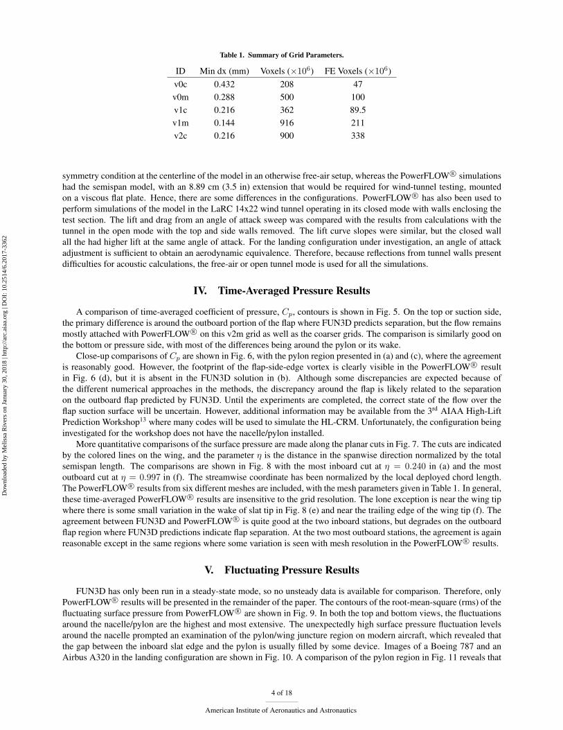
Table 1. Summary of Grid Parameters.
ID Min dx (mm) Voxels (×106) FE Voxels (×10
6)
v0c 0.432 208 47
v0m 0.288 500 100
v1c 0.216 362 89.5
v1m 0.144 916 211
v2c 0.216 900 338
symmetry condition at the centerline of the model in an otherwise free-air setup, whereas the PowerFLOW R© simulations
had the semispan model, with an 8.89 cm (3.5 in) extension that would be required for wind-tunnel testing, mounted
on a viscous flat plate. Hence, there are some differences in the configurations. PowerFLOW R© has also been used to
perform simulations of the model in the LaRC 14x22 wind tunnel operating in its closed mode with walls enclosing the
test section. The lift and drag from an angle of attack sweep was compared with the results from calculations with the
tunnel in the open mode with the top and side walls removed. The lift curve slopes were similar, but the closed wall
all the had higher lift at the same angle of attack. For the landing configuration under investigation, an angle of attack
adjustment is sufficient to obtain an aerodynamic equivalence. Therefore, because reflections from tunnel walls present
difficulties for acoustic calculations, the free-air or open tunnel mode is used for all the simulations.
IV. Time-Averaged Pressure Results
A comparison of time-averaged coefficient of pressure, Cp, contours is shown in Fig. 5. On the top or suction side,
the primary difference is around the outboard portion of the flap where FUN3D predicts separation, but the flow remains
mostly attached with PowerFLOW R© on this v2m grid as well as the coarser grids. The comparison is similarly good on
the bottom or pressure side, with most of the differences being around the pylon or its wake.
Close-up comparisons of Cp are shown in Fig. 6, with the pylon region presented in (a) and (c), where the agreement
is reasonably good. However, the footprint of the flap-side-edge vortex is clearly visible in the PowerFLOW R© result
in Fig. 6 (d), but it is absent in the FUN3D solution in (b). Although some discrepancies are expected because of
the different numerical approaches in the methods, the discrepancy around the flap is likely related to the separation
on the outboard flap predicted by FUN3D. Until the experiments are completed, the correct state of the flow over the
flap suction surface will be uncertain. However, additional information may be available from the 3rd AIAA High-Lift
Prediction Workshop13 where many codes will be used to simulate the HL-CRM. Unfortunately, the configuration being
investigated for the workshop does not have the nacelle/pylon installed.
More quantitative comparisons of the surface pressure are made along the planar cuts in Fig. 7. The cuts are indicated
by the colored lines on the wing, and the parameter η is the distance in the spanwise direction normalized by the total
semispan length. The comparisons are shown in Fig. 8 with the most inboard cut at η = 0.240 in (a) and the most
outboard cut at η = 0.997 in (f). The streamwise coordinate has been normalized by the local deployed chord length.
The PowerFLOW R© results from six different meshes are included, with the mesh parameters given in Table 1. In general,
these time-averaged PowerFLOW R© results are insensitive to the grid resolution. The lone exception is near the wing tip
where there is some small variation in the wake of slat tip in Fig. 8 (e) and near the trailing edge of the wing tip (f). The
agreement between FUN3D and PowerFLOW R© is quite good at the two inboard stations, but degrades on the outboard
flap region where FUN3D predictions indicate flap separation. At the two most outboard stations, the agreement is again
reasonable except in the same regions where some variation is seen with mesh resolution in the PowerFLOW R© results.
V. Fluctuating Pressure Results
FUN3D has only been run in a steady-state mode, so no unsteady data is available for comparison. Therefore, only
PowerFLOW R© results will be presented in the remainder of the paper. The contours of the root-mean-square (rms) of the
fluctuating surface pressure from PowerFLOW R© are shown in Fig. 9. In both the top and bottom views, the fluctuations
around the nacelle/pylon are the highest and most extensive. The unexpectedly high surface pressure fluctuation levels
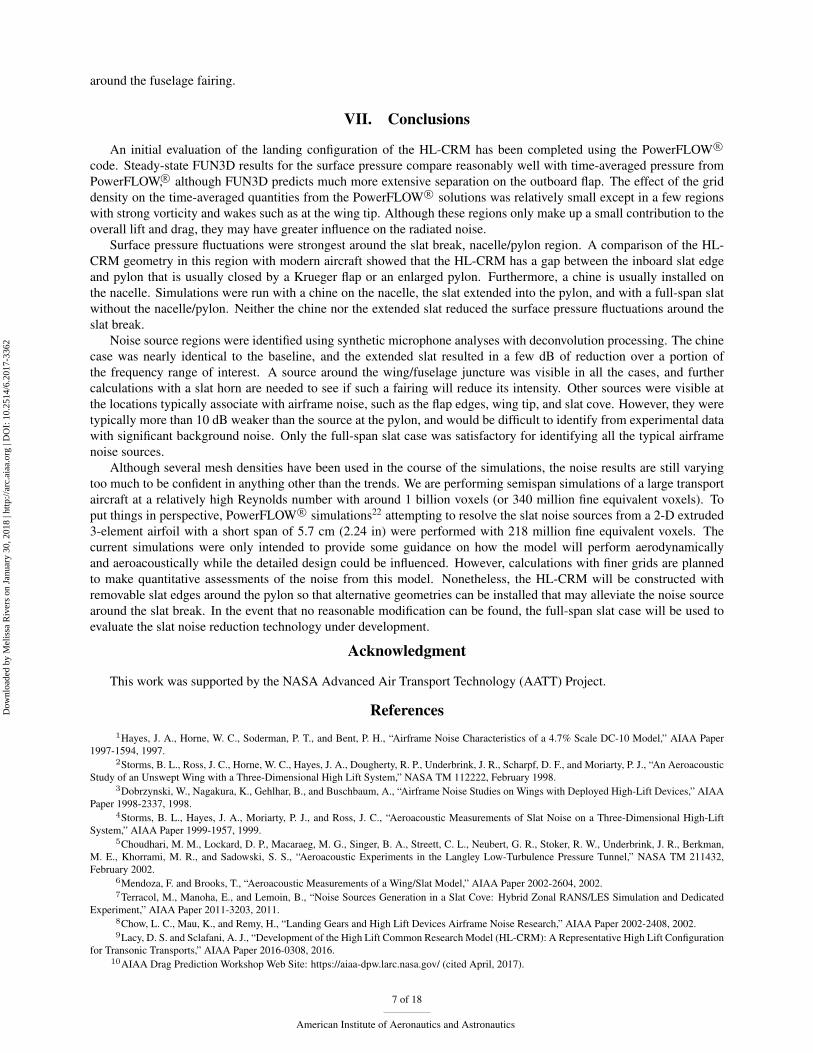
around the nacelle prompted an examination of the pylon/wing juncture region on modern aircraft, which revealed that
the gap between the inboard slat edge and the pylon is usually filled by some device. Images of a Boeing 787 and an
Airbus A320 in the landing configuration are shown in Fig. 10. A comparison of the pylon region in Fig. 11 reveals that
4 of 18
American Institute of Aeronautics and Astronautics
Dow
nloa
ded
by M
elis
sa R
iver
s on
Jan
uary
30,
201
8 | h
ttp://
arc.
aiaa
.org
| D
OI:
10.
2514
/6.2
017-
3362

an important difference between the configurations involves the presence of a Krueger flap between the inboard slat and
the pylon on the Boeing 787 and a bulge in the pylon on the A320 that closes the gap with the inboard slat. Curiously,
we have not found any aircraft where the gap between the outboard slat and the pylon is closed in a similar fashion.
Another obvious difference is the relatively narrow and more rectangular pylon on the HL-CRM in comparison with
the two real aircraft. The pylon and gap treatments on real aircraft are most likely designed for aerodynamic reasons,
but they are also likely to have an important effect on the acoustics. One of the goals of the upcoming HL-CRM test is
to examine slat-cove noise reduction devices, and minimizing other sources, especially those that are unrealistic, which
will make it easier to isolate true slat-cove noise. Therefore, additional PowerFLOW R© calculations have been performed
with a nacelle chine, with the slat extended into the pylon, and with a full-span slat and no nacelle/pylon. All of these
simulations were run with meshes similar to the v2c grid for the baseline geometry. The nacelle chine was taken from
another aircraft geometry of a similar sized aircraft, but may not be identical to the chine that is ultimately designed for
the HL-CRM. Furthermore, only three locations of the chine were evaluated at an angle of attack of 8,◦ and the position
where the vortex coming off the chine most closely passed through the slat break region was chosen for an additional
simulation. However, this may not be an optimal position for the stall case, i.e., the primary target for the employment
of a chine.
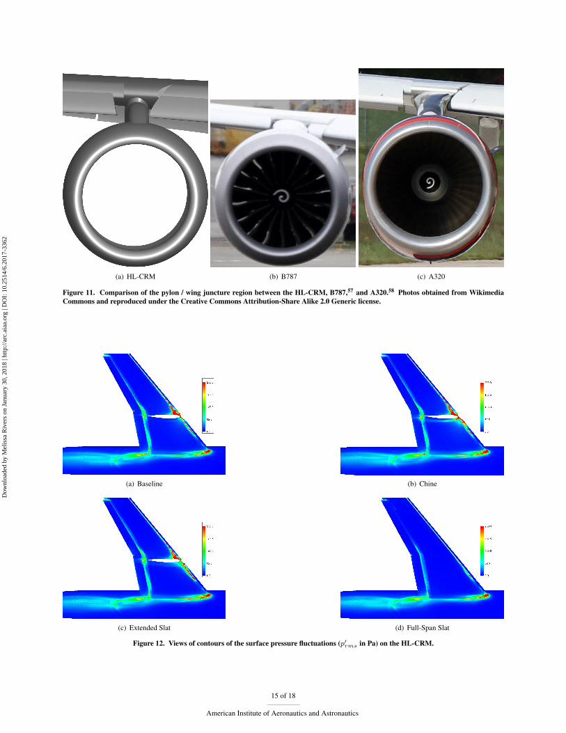
The rms of the perturbation pressure from the four simulations is shown in Fig. 12. The nacelle and pylon have
been removed to allow a direct view of the slat break region. The chine has very little effect on the fluctuations, and
the extended slat has more pronounced fluctuations on the inboard slat near the slat break. As should be expected, the
full-span slat case has much lower fluctuation levels on the slat. All of the simulations exhibit significant unsteadiness
near the wing-fuselage junction, but the current version of the HL-CRM does not have a slat horn or fairing that would
have smoothed out the flow in this region. Fluctuations are also seen around the inboard flap edge and the fuselage.
Some of this is caused by the flow around the flap edge, but some is because of the fuselage fairing, which is not readily
apparent in the figure. The fuselage fairing is not very well resolved and some of the unsteadiness may disappear with
grid refinement in this region. Additional regions with significant fluctuation levels include the outboard flap tip and the
main wing cove, especially in the wake of the pylon. The fluctuation levels in the main cove were observed to increase
significantly after refining the grid in the wake of the slat edges adjacent to the pylon.
Close-up views of the nacelle/pylon are presented in Fig. 13 where now the case with the chine exhibits some subtle
differences with the baseline. Surface streamlines have been superimposed on the contours to give another indication of
the flow patterns. Again, the extended slat case appears to have enhanced fluctuation levels both on the slat and nacelle.
The extended slat presents more blockage to the flow, so the fluid has to accelerate more to get around the pylon. The
higher velocities may be partially responsible for the higher fluctuations. Another view of this region is presented in
Fig. 14 where the complicated flow patterns and stagnation regions around the pylon are readily apparent in the surface
streamlines. In contrast, the flow around the full-span slat is fairly uniform in the span and does not exhibit any regions
with higher fluctuation levels as those seen in the three other cases.
The results from all the simulations were relatively similar around most of the model, so only the results from the
baseline case are presented for some other important regions in Fig. 15. The top of the wing tip is shown in Fig. 15
(a), where the wake of the slat tip is evident. Only a small portion of the fluctuations are really from the slat edge as
considerable separation also occurs on the edge created by the unslatted portion of the main element. After sufficient
grid refinement, this vortical feature persisted so that its footprint was visible to the trailing edge of the wing. Significant
fluctuations are also visible at the trailing edge near the wing tip. The wing tip vortex migrates from the side to the top
at around the 80% chord position and is still relatively close to the wing surface as it moves across the trailing edge. The
fluctuations near the leading edge of the wing tip are more visible in Fig. 15 (b) and are associated with disturbances in
the slat cove being carried out past the slat edge by a strong spanwise flow and then being wrapped around the wing tip.
An additional region with significant fluctuation levels includes the outboard flap edge shown in Fig. 15 (c). A typical
dual vortex system is observed where the side-edge vortex migrates to the top around the 60% chord position and merges
with the upper surface vortex. The last region examined is around the wing/fuselage junction shown in Fig. 9 (d) where
high fluctuation levels are observed just upstream of the wing and around the edge created by the unslatted portion of
the main element.
VI. Acoustics: Synthetic Array Beamforming
Although the simulations indicate strong unsteadiness in several locations on the model, the rms levels include
fluctuations at all frequencies. Some very low frequency oscillations may be present in the pressure signals and may
even dominate the rms levels. These are not particularly relevant for acoustics and, hence, contours focused on just the
rms pressure fluctuations can be misleading. Even without this contamination, only a small fraction of fluctuating energy
5 of 18
American Institute of Aeronautics and Astronautics
Dow
nloa
ded
by M
elis
sa R
iver
s on
Jan
uary
30,
201
8 | h
ttp://
arc.
aiaa
.org
| D
OI:
10.
2514
/6.2
017-
3362

is actually converted into acoustics. Hence, for any frequency, the rms pressure levels can only give an indication of
potential noise source locations. One method to assess actual noise sources is through array beamforming. Conventional
beamforming involves assuming an acoustic source basis function (such as a monopole in a uniform flow) and placing
one of these sources at every point in a mesh surrounding a region where sound sources are expected. A source strength
amplitude for each grid point is determined by how well cross-correlations of the signals across the microphone array
are consistent with those based on the assumed basis function. Using the distances between the grid point and the
microphones, each signal is adjusted in amplitude and time (or phase). They can then be combined such that the
portion of the signal consistent with the assumed basis adds up constructively, whereas the inconsistent portion combines
destructively. However, this assumes that the sources are uncorrelated and that their directivity is consistent with that
of the basis function, which is typically a monopole. Furthermore, even when the source coincides exactly with the
assumed basis, the array response is dependent on the particular arrangement of the microphones relative to the sources.
Deconvolution methods have been developed to account for the array response that can provide spectra equivalent to what
would be obtained by a single microphone, but all of these algorithms require certain assumptions and some of them can
be computationally expensive. Nonetheless, microphone arrays have provided valuable information about noise sources
when the elevated background noise would render single microphone measurements useless. In particular, the contour
maps of source strength provide information about the location of sources that was not available previously. Array
beamforming is typically used with experimental data, but the technique is now being applied to numerical simulation
data.49, 50
A methodology commonly used to make aeroacoustic predictions using CFD involves coupling the near-field solution
from the CFD to an acoustic analogy such as the Ffowcs Williams and Hawking’s equation51 (FW-H). These predictions
are often computed at the center of a microphone array and compared with the array output. However, with a minimal
increase in computational cost, the predictions can be made at all microphone locations in an array, and the signals
processed in the same manner as experimental data. Hence, the simulations provide synthetic array data that can be used
with beamforming techniques.
The far-field noise from the HL-CRM was calculated using the FW-H equation51, 52 solver described by Bres.53
Results were obtained using 0.4 seconds of pressure time history data on all solid surfaces on the model but not on the
flat plate. The array is positioned in the 90◦ position, geometrically directly beneath the center of the wing. The 97-
microphone array is 276 inches (7 m) from the model centerline, with an outer diameter (microphone to microphone) of
78.6 inches (2.0 m). An array shading algorithm was employed to exclude certain microphones based on the frequency
so that sources appear similar in size across the frequency range and to reduce the distances between the included
microphones as the frequency increases, which helps to minimize the detrimental effects of decorrelation. The array
data was processed using the Exa beamforming code that uses the CLEAN-SC54 deconvolution approach. Detailed
information about the array and processing procedure are in Refs. 14 and 50.
CLEAN-SC beamform maps are shown in Fig. 16 for the four configurations under investigation. The data was
processed in narrow band with a bin width of 125 Hz. The contour levels are normalized by the maximum for that
map, and the range is 20 dB. Hence, only the relative distribution of source levels should be compared between the
four cases. However, the baseline and chine cases are nearly identical with the extended slat being a few dB quieter for
frequencies below 1 kHz and above 4 kHz. The full-span slat case is around 10 dB quieter than the baseline over almost
all frequencies, with the exceptions being at 2 and 2.5 kHz where tones are present in the full-span slat spectra. As seen
in Fig. 16, the source of the tone is associated with the outer section of the outboard slat. A similar source location was
observed in the experimental testing of a 26% 777 model19, 55 and in a flight test.56 In the current simulations, the tones
appear to be reminiscent of the narrow band peaks observed in many small-scale slat experiments and accompanying
computations. The particular geometric arrangement and flow in the outboard section of the slat may lend itself to the
narrow band peak phenonema. However, the current model does not have any brackets, which may alter the flow and
have an impact on these tones. The three other cases in Fig. 16 are dominated by a source around the pylon, with the
other sources being 10 dB down. Although the secondary sources are evident in these results, they may be difficult to
observe in an experiment because of much higher background noise levels. The secondary noise sources include the
wing tip, outboard flap edge, and slat break wake on the upper surface of the wing interacting with the main flap cove.
This last source is the one seen on the inboard flap. The tonal slat source is not observed in the cases with the pylon
because they do not have as much resolution in the slat cove. An additional simulation of the baseline with increased
slat cove resolution has been completed, and the same slat tone phenomenon was evident.
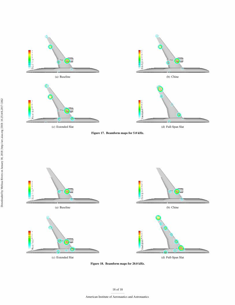
At a frequency of 5.0 kHz, Fig. 17 shows that the outboard flap edge source is now stronger than the one near the
wing tip, but the pylon is still dominant. A source at the wing/fuselage junction is now more apparent as well. The maps
for 20.0 kHz in Fig. 18 are indicative of those for the remainder of the frequency range up to 30 kHz. The pylon region
persists as a strong source, but the wing tip and outboard flap are visible for the two quieter cases. Extensive sources are
now visible on the fuselage for the full-span slat case, and we believe that these may be a result of insufficient resolution
6 of 18
American Institute of Aeronautics and Astronautics
Dow
nloa
ded
by M
elis
sa R
iver
s on
Jan
uary
30,
201
8 | h
ttp://
arc.
aiaa
.org
| D
OI:
10.
2514
/6.2
017-
3362
around the fuselage fairing.
VII. Conclusions
An initial evaluation of the landing configuration of the HL-CRM has been completed using the PowerFLOW R©
code. Steady-state FUN3D results for the surface pressure compare reasonably well with time-averaged pressure from
PowerFLOW,R© although FUN3D predicts much more extensive separation on the outboard flap. The effect of the grid
density on the time-averaged quantities from the PowerFLOW R© solutions was relatively small except in a few regions
with strong vorticity and wakes such as at the wing tip. Although these regions only make up a small contribution to the
overall lift and drag, they may have greater influence on the radiated noise.
Surface pressure fluctuations were strongest around the slat break, nacelle/pylon region. A comparison of the HL-
CRM geometry in this region with modern aircraft showed that the HL-CRM has a gap between the inboard slat edge
and pylon that is usually closed by a Krueger flap or an enlarged pylon. Furthermore, a chine is usually installed on
the nacelle. Simulations were run with a chine on the nacelle, the slat extended into the pylon, and with a full-span slat
without the nacelle/pylon. Neither the chine nor the extended slat reduced the surface pressure fluctuations around the
slat break.
Noise source regions were identified using synthetic microphone analyses with deconvolution processing. The chine
case was nearly identical to the baseline, and the extended slat resulted in a few dB of reduction over a portion of
the frequency range of interest. A source around the wing/fuselage juncture was visible in all the cases, and further
calculations with a slat horn are needed to see if such a fairing will reduce its intensity. Other sources were visible at
the locations typically associate with airframe noise, such as the flap edges, wing tip, and slat cove. However, they were
typically more than 10 dB weaker than the source at the pylon, and would be difficult to identify from experimental data
with significant background noise. Only the full-span slat case was satisfactory for identifying all the typical airframe
noise sources.
Although several mesh densities have been used in the course of the simulations, the noise results are still varying
too much to be confident in anything other than the trends. We are performing semispan simulations of a large transport
aircraft at a relatively high Reynolds number with around 1 billion voxels (or 340 million fine equivalent voxels). To
put things in perspective, PowerFLOW R© simulations22 attempting to resolve the slat noise sources from a 2-D extruded
3-element airfoil with a short span of 5.7 cm (2.24 in) were performed with 218 million fine equivalent voxels. The
current simulations were only intended to provide some guidance on how the model will perform aerodynamically
and aeroacoustically while the detailed design could be influenced. However, calculations with finer grids are planned
to make quantitative assessments of the noise from this model. Nonetheless, the HL-CRM will be constructed with
removable slat edges around the pylon so that alternative geometries can be installed that may alleviate the noise source
around the slat break. In the event that no reasonable modification can be found, the full-span slat case will be used to
evaluate the slat noise reduction technology under development.
Acknowledgment
This work was supported by the NASA Advanced Air Transport Technology (AATT) Project.
References
1Hayes, J. A., Horne, W. C., Soderman, P. T., and Bent, P. H., “Airframe Noise Characteristics of a 4.7% Scale DC-10 Model,” AIAA Paper
1997-1594, 1997.2Storms, B. L., Ross, J. C., Horne, W. C., Hayes, J. A., Dougherty, R. P., Underbrink, J. R., Scharpf, D. F., and Moriarty, P. J., “An Aeroacoustic
Study of an Unswept Wing with a Three-Dimensional High Lift System,” NASA TM 112222, February 1998.3Dobrzynski, W., Nagakura, K., Gehlhar, B., and Buschbaum, A., “Airframe Noise Studies on Wings with Deployed High-Lift Devices,” AIAA
Paper 1998-2337, 1998.4Storms, B. L., Hayes, J. A., Moriarty, P. J., and Ross, J. C., “Aeroacoustic Measurements of Slat Noise on a Three-Dimensional High-Lift
System,” AIAA Paper 1999-1957, 1999.5Choudhari, M. M., Lockard, D. P., Macaraeg, M. G., Singer, B. A., Streett, C. L., Neubert, G. R., Stoker, R. W., Underbrink, J. R., Berkman,
M. E., Khorrami, M. R., and Sadowski, S. S., “Aeroacoustic Experiments in the Langley Low-Turbulence Pressure Tunnel,” NASA TM 211432,
February 2002.6Mendoza, F. and Brooks, T., “Aeroacoustic Measurements of a Wing/Slat Model,” AIAA Paper 2002-2604, 2002.7Terracol, M., Manoha, E., and Lemoin, B., “Noise Sources Generation in a Slat Cove: Hybrid Zonal RANS/LES Simulation and Dedicated
Experiment,” AIAA Paper 2011-3203, 2011.8Chow, L. C., Mau, K., and Remy, H., “Landing Gears and High Lift Devices Airframe Noise Research,” AIAA Paper 2002-2408, 2002.9Lacy, D. S. and Sclafani, A. J., “Development of the High Lift Common Research Model (HL-CRM): A Representative High Lift Configuration
for Transonic Transports,” AIAA Paper 2016-0308, 2016.10AIAA Drag Prediction Workshop Web Site: https://aiaa-dpw.larc.nasa.gov/ (cited April, 2017).
7 of 18
American Institute of Aeronautics and Astronautics
Dow
nloa
ded
by M
elis
sa R
iver
s on
Jan
uary
30,
201
8 | h
ttp://
arc.
aiaa
.org
| D
OI:
10.
2514
/6.2
017-
3362

11NASA Common Research Model Web Site: https://commonresearchmodel.larc.nasa.gov/ (cited April, 2017).12AIAA Geometry and Mesh Generation Web Site: http://www.pointwise.com/gmgw/ (cited April, 2017).13AIAA High Lift Prediction Workshop: https://hiliftpw.larc.nasa.gov/ (cited April, 2017).14Humphreys, W. M., Brooks, T. F., Bahr, C. J., Spalt, T. B., Bartram, S. M., Culliton, W., and Becker, L., “Development of a Microphone Phased
Array Capability for the Langley 14- by 22-foot Subsonic Tunnel,” AIAA Paper 2014-2343, 2014.15Khorrami, M. R., Humphreys, W. M., Lockard, D. P., and Ravetta, P. A., “Aeroacoustic Evaluation of Flap and Landing Gear Noise Reduction
Concepts,” AIAA Paper 2014-2478, 2014.16Streett, C. L., Casper, J., Lockard, D. P., Khorrami, M. R., Stoker, R., Elkoby, R., Wenneman, W., and Underbrink, J., “Aerodynamic Noise
Reduction for High-Lift Devices on a Swept Wing Model,” AIAA Paper 2006-0212, 2006.17Scholten, W. D., Hartl, D. J., Turner, T. L., and Kidd, R. T., “Development and Analysis-Driven Optimization of Superelastic Slat-Cove Fillers
for Airframe Noise Reduction,” AIAA Journal, Vol. 54, No. 3, 2016, pp. 1078–1094.18Turner, T. L. and Long, D. L., “Development of a SMA-Based, Slat-Gap Filler for Airframe Noise Reduction,” AIAA Paper 2015-0730, 2015.19Horne, W. C., Burnside, N. J., Soderman, P. T., Jaeger, S. M., Reinero, B. R., James, K. D., and Arledge, T. K., “Aeroacoustic Study of a
26%-Scale Semispan Model of a Boeing 777 Wing in the NASA Ames 40- by 80-Foot Wind Tunnel,” NASA TP 2004-212802, October 2004.20Fares, E., Casalino, D., and Khorrami, M., “Evaluation of Airframe Noise Reduction Concepts via Simulations Using a Lattice Boltzmann
Approach,” AIAA Paper 2015-2988, 2015.21Khorrami, M. R., Humphreys, W. M., Lockard, D. P., and Ravetta, P. A., “An Assessment of Flap and Main Landing Gear Noise Abatement
Concepts,” AIAA Paper 2015-2978, 2015.22Choudhari, M. M. and Lockard, D. P., “Assessment of Slat Noise Predictions for 30P30N High-Lift Configuration from BANC-III Workshop,”
AIAA Paper 2015-2844, 2015.23Rivers, M., Hunter, C., and Vatsa, V., “Computational Fluid Dynamic Analyses for the High-Lift Common Research Model Using the USM3D
and FUN3D Flow Solvers,” AIAA Paper 2017-0320, 2017.24Biedron, R. T., Derlaga, J. M., Gnoffo, P. A., Hammond, D. P., Jones, W. T., Kleb, B., Lee-Rausch, E. M., Nielsen, E. J., Park, M. A., Rumsey,
C. L., Thomas, J. L., , and Wood, W. A., “FUN3D Manual: 12.4,” NASA TM 2014-218179, March 2014.25Chen, H., “Volumetric Formulation of the Lattice Boltzmann Method for Fluid Dynamics: Basic Concept,” Physical Review A, Vol. 58,
September 1998, pp. 3955–3963.26Chen, H., Teixeira, C., and Molvig, K., “Realization of Fluid Boundary Conditions via Discrete Boltzmann Dynamics,” Intl. J. Mod. phys. C,
Vol. 9, No. 8, 1998, pp. 1281–1292.27Yakhot, V. and Orszag, S., “Renormalization Group Analysis of Turbulence. I. Basic Theory,” J. Sci. Comput., Vol. 1, No. 2, 1986, pp. 3–51.28Chen, H., Kandasamy, S., Orszag, S., Shock, R., Succi, S., and Yakhot, V., “Extended Boltzmann Kinetic Equation for Turbulent Flows,”
Science, Vol. 301, No. 5633, 2003, pp. 633–636.29Chen, S. and Doolen, G., “Lattice Boltzmann Method for Fluid Flows,” Annu. Rev. Fluid Mech., Vol. 30, January 1998, pp. 329–364.30Fares, E. and Nolting, S., “Unsteady Flow Simulation of a High-Lift Configuration using a Lattice Boltzmann Approach,” AIAA Paper 2011-
869, 2011.31Khorrami, M., Fares, E., and Casalino, D., “Towards Full-Aircraft Airframe Noise Prediction: Lattice-Boltzmann Simulations,” AIAA Paper
2014-2481, 2014.32Chen, H., Chen, S., and Matthaeus, W., “Recovery of the Navier-Stokes Equations Using a Lattice-gas Boltzmann Method,” Physical Review
A, Vol. 45, 1992, pp. 5339–5342.33Qiana, Y. H., D’Humieres, D., and Lallemand, P., “Lattice BGK Models for Navier-Stokes Equations,” Europhysics Letters, Vol. 17, 1992,
pp. 479–484.34Marie, S., Ricot, D., and Sagaut, P., “Comparison between Lattice Boltzmann Method and Navier-Stokes High Order Schemes for Computa-
tional Aeroacoustics,” J. of Computational Physics, Vol. 228, 2009, pp. 1056–1070.35Bres, G., Perot, F., and Freed, D., “Properties of the Lattice-Boltzmann Method for Acoustics,” AIAA Paper 2009-3395, 2009.36Lockard, D., “Summary of the Tandem Cylinder Solutions from the Benchmark problems for Airframe Noise Computations-I Workshop,”
AIAA Paper 2011-353, 2011.37Shan, X., Yuvan, X.-F., and Chen, H., “Kinetic Theory Representation of Hydrodynamics: a Way Beyond the Navier-Stokes Equation,” Physics.
Rev. Lett., Vol. 80, 1998, pp. 65–88.38Zhuo, C., Zhong, C., Li, K., Xiong, S., Chen, X., and Cao, J., “Application of Lattice Boltzmann Method to Simulation of Compressible
Turbulent Flow,” Commun. Comput. Physics, Vol. 8, 2010, pp. 1208–1223.39Fares, E., Wessels, M., Li, Y., Gopalakrishnan, P., Zhang, R., Sun, C., Gopalaswamy, N., Roberts, P., Hoch, J., and Chen, H., “Validation of a
Lattice Boltzmann Approach for Transonic and Supersonic Simulations,” AIAA Paper 2014-0952, 2014.40Koeing, B. and Fares, E., “Validation of a Transonic Lattice-Boltzmann Method for the NASA Common Research Model,” AIAA Paper
2016-2023, 2016.41Duda, B., Fares, E., Wessels, M., and Vatsa, V., “Unsteady Flow Simulation of a Sweepig Jet Actuator Using a Lattice-Boltzmann Method,”
AIAA Paper 2016-1818, 2016.42Li, Y., Shock, R., and Chen, H., “Numerical Study of Flow Past an Impulsively Started Cylinder by Lattice Botzmann Method,” J. Fluid Mech.,
Vol. 519, November 2004, pp. 273–300.43Chen, H., Orszag, S., Staroselsky, I., and Succi, S., “Expanded Analogy between Boltzmann Kinetic Theory of Fluid and Turbulence,” J. Fluid
Mech., Vol. 519, November 2004, pp. 301–314.44Fares, E., “Unsteady Flow Simulation of the Ahmed Reference Body using a Lattice Boltzmann Approach,” Comput. Fluids, Vol. 35, No. 8-9,
2006, pp. 940–950.45Bres, G., Fares, E., Williams, D., and Colonius, T., “Numerical Simulations of the Transient Flow Response of a 3D, Low-Aspect-Ratio Wing
to Pulsed Actuation,” AIAA Paper 2011-3440, 2011.46Bres, G., Freed, D., Wessels, M., Noelting, M., and Perot, F., “Flow and Noise Predictions for Tandem Cylinder Aeroacoustic Benchmark,”
Physics of Fluids, Vol. 24, No. 3, 2012, http://dx.doi.org/10.1063/1.3685102.
8 of 18
American Institute of Aeronautics and Astronautics
Dow
nloa
ded
by M
elis
sa R
iver
s on
Jan
uary
30,
201
8 | h
ttp://
arc.
aiaa
.org
| D
OI:
10.
2514
/6.2
017-
3362

47Casalino, D., Ribeiro, A., and Fares, E., “Facing Rim Cavities Fluctuation Modes,” Journal of Sound and Vibration, Vol. 333, No. 13, 2014,
pp. 2812–2830.48Spalart, P. R. and Allmaras, S., “A One-Equation Turbulence Model for Aerodynamic Flows,” Recherche Aerospatiale, Vol. 1, No. 1, 1994,
pp. 5–21.49Marotta, T. R., Lieber, L. S., and Dougherty, R. P., “Validation of Beamforming Analysis Methodology with Synthesized Acoustic Time History
Data: Sub-Scale Fan Rig System,” AIAA Paper 2014-3068, 2014.50Lockard, D. P., Humphreys, W. M., Khorrami, M. R., Fares, E., Casalino, D., and Ravetta, P. A., “Comparison of Computational and Experi-
mental Microphone Array Results for an 18%-Scale Aircraft Model,” AIAA Paper 2015-2990, 2015.51Ffowcs Williams, J. E. and Hawkings, D. L., “Sound Generation by Turbulence and Surfaces in Arbitrary Motion,” Philosophical Transactions
of the Royal Society, Vol. A264, No. 1151, 1969, pp. 321–342.52Najafi-Yazdi, A., Bres, G. A., and Mongeau, L., “An Acoustic Analogy Formulation for Moving Sources in Uniformly Moving Media,”
Proceedings of the Royal Society of London, Series A, Vol. 467, No. 2125, 2011, pp. 144–165.53Bres, G. A., Wessels, M., and Noelting, S., “Tandem Cylinder Noise Predictions Using Lattice Boltzmann and Ffowcs Williams – Hawkings
Methods,” AIAA Paper 2010-3791, 2010.54Sijtsma, P., “CLEAN Based on Spatial Source Coherence,” AIAA Paper 2007-3436, 2014.55Horne, W. C., James, K. D., Arledge, T. K., and Soderman, P. T., “Measurements of a 26%-Scale 777 Airframe Noise in the NASA Ames 40-
by 80-Foot Wind Tunnel,” AIAA Paper 2005-2810, 2005.56Stoker, R., Guo, Y., Streett, C., and Burnside, N., “Airframe Noise Source Locations of a 777 Aircraft in Flight and Comparisons with Past
Model-Scale Tests,” AIAA Paper 2003-3111, 2003.57Salard, E., “American Airlines, Boeing 787-8 Dreamliner, N805AN - PAE (18677833553),”
https://commons.wikimedia.org/wiki/File:American Airlines, Boeing 787-8 Dreamliner, N805AN - PAE (18677833553).jpg,
https://creativecommons.org/licenses/by-sa/2.0/de/legalcode, 2015.58Strey, B., “Aeroflot A320 front view,” https://commons.wikimedia.org/wiki/File:Aeroflot A320 front view.jpg,
https://creativecommons.org/licenses/by-sa/2.0/legalcode, 2011.
(a) Top view (b) Front view
Figure 1. Two views of the HL-CRM geometry.
Figure 2. PowerFLOW R© grid distribution on a plane through the HL-CRM.
9 of 18
American Institute of Aeronautics and Astronautics
Dow
nloa
ded
by M
elis
sa R
iver
s on
Jan
uary
30,
201
8 | h
ttp://
arc.
aiaa
.org
| D
OI:
10.
2514
/6.2
017-
3362

(a) Top (b) Bottom
Figure 3. Identification of some of the variable resolution regions on the HL-CRM.
(a) v0m Pylon (b) v0m Wing Tip
(c) v2m Pylon (d) v2m Wing Tip
Figure 4. PowerFLOW R© grid distribution on planes through the HL-CRM.
10 of 18
American Institute of Aeronautics and Astronautics
Dow
nloa
ded
by M
elis
sa R
iver
s on
Jan
uary
30,
201
8 | h
ttp://
arc.
aiaa
.org
| D
OI:
10.
2514
/6.2
017-
3362

(a) FUN3D Top (b) FUN3D Bottom
(c) PowerFLOW R© Top (d) PowerFLOW R© Bottom
Figure 5. Contours of the mean Cp on the HL-CRM. PowerFLOW R© results from v2m mesh.
11 of 18
American Institute of Aeronautics and Astronautics
Dow
nloa
ded
by M
elis
sa R
iver
s on
Jan
uary
30,
201
8 | h
ttp://
arc.
aiaa
.org
| D
OI:
10.
2514
/6.2
017-
3362

(a) FUN3D pylon (b) FUN3D outboard flap
(c) PowerFLOW R© pylon (d) PowerFLOW R© outboard flap
Figure 6. Contours of the mean Cp on parts of the HL-CRM.
Figure 7. Planar cuts along the wing used for comparisons.
12 of 18
American Institute of Aeronautics and Astronautics
Dow
nloa
ded
by M
elis
sa R
iver
s on
Jan
uary
30,
201
8 | h
ttp://
arc.
aiaa
.org
| D
OI:
10.
2514
/6.2
017-
3362

x/c
Cp
0 0.2 0.4 0.6 0.8 1
-3
-2
-1
0
1
FUN3Dv0cv0mv1cv1mv2c
Powerflow
(a) η = 0.240
x/c
Cp
0 0.2 0.4 0.6 0.8 1
-3
-2
-1
0
1
FUN3Dv0cv0mv1cv1mv2c
Powerflow
(b) η = 0.418
x/c
Cp
0 0.2 0.4 0.6 0.8 1
-3
-2
-1
0
1
FUN3Dv0cv0mv1cv1mv2c
Powerflow
(c) η = 0.552
x/c
Cp
0 0.2 0.4 0.6 0.8 1
-3
-2
-1
0
1
FUN3Dv0cv0mv1cv1mv2c
Powerflow
(d) η = 0.819
x/c
Cp
0 0.2 0.4 0.6 0.8 1
-4
-3
-2
-1
0
1
FUN3Dv0cv0mv1cv1mv2c
Powerflow
(e) η = 0.966
x/c
Cp
0 0.2 0.4 0.6 0.8 1
-4
-3
-2
-1
0
1
FUN3Dv0cv0mv1cv1mv2c
Powerflow
(f) η = 0.997
Figure 8. Cp on planar cuts through the HL-CRM wing.
13 of 18
American Institute of Aeronautics and Astronautics
Dow
nloa
ded
by M
elis
sa R
iver
s on
Jan
uary
30,
201
8 | h
ttp://
arc.
aiaa
.org
| D
OI:
10.
2514
/6.2
017-
3362

(a) Top view (b) Bottom view
Figure 9. Contours of the surface pressure fluctuations (p′rms
in Pa) on the HL-CRM.
(a) B787 (b) A320
Figure 10. Images of modern B78757 and A32058 aircraft in the landing configuration. Photos obtained from Wikimedia Commons and
reproduced under the Creative Commons Attribution-Share Alike 2.0 Generic license.
14 of 18
American Institute of Aeronautics and Astronautics
Dow
nloa
ded
by M
elis
sa R
iver
s on
Jan
uary
30,
201
8 | h
ttp://
arc.
aiaa
.org
| D
OI:
10.
2514
/6.2
017-
3362
(a) HL-CRM (b) B787 (c) A320
Figure 11. Comparison of the pylon / wing juncture region between the HL-CRM, B787,57 and A320.58 Photos obtained from Wikimedia
Commons and reproduced under the Creative Commons Attribution-Share Alike 2.0 Generic license.
(a) Baseline (b) Chine
(c) Extended Slat (d) Full-Span Slat
Figure 12. Views of contours of the surface pressure fluctuations (p′rms
in Pa) on the HL-CRM.
15 of 18
American Institute of Aeronautics and Astronautics
Dow
nloa
ded
by M
elis
sa R
iver
s on
Jan
uary
30,
201
8 | h
ttp://
arc.
aiaa
.org
| D
OI:
10.
2514
/6.2
017-
3362

(a) Baseline (b) Chine
(c) Extended Slat (d) Full-Span Slat
Figure 13. Close-up views of contours of the surface pressure fluctuations (p′rms
in Pa) on the nacelle/pylon of the HL-CRM.
(a) Baseline (b) Chine
(c) Extended Slat (d) Full-Span Slat
Figure 14. Close-up views of contours of the surface pressure fluctuations (p′rms
in Pa) on the pylon of the HL-CRM.
16 of 18
American Institute of Aeronautics and Astronautics
Dow
nloa
ded
by M
elis
sa R
iver
s on
Jan
uary
30,
201
8 | h
ttp://
arc.
aiaa
.org
| D
OI:
10.
2514
/6.2
017-
3362

(a) Wing Tip (b) Top of Wing Tip
(c) Outboard Flap Edge (d) Wing/Fuselage Junction
Figure 15. Views of contours of the surface pressure fluctuations (p′rms
in Pa) on the HL-CRM.
(a) Baseline (b) Chine
(c) Extended Slat (d) Full-Span Slat
Figure 16. Beamform maps for 2.5 kHz.
17 of 18
American Institute of Aeronautics and Astronautics
Dow
nloa
ded
by M
elis
sa R
iver
s on
Jan
uary
30,
201
8 | h
ttp://
arc.
aiaa
.org
| D
OI:
10.
2514
/6.2
017-
3362
(a) Baseline (b) Chine
(c) Extended Slat (d) Full-Span Slat
Figure 17. Beamform maps for 5.0 kHz.
(a) Baseline (b) Chine
(c) Extended Slat (d) Full-Span Slat
Figure 18. Beamform maps for 20.0 kHz.
18 of 18
American Institute of Aeronautics and Astronautics
Dow
nloa
ded
by M
elis
sa R
iver
s on
Jan
uary
30,
201
8 | h
ttp://
arc.
aiaa
.org
| D
OI:
10.
2514
/6.2
017-
3362