Noise updating repeated Wiener filter and other adaptive noise smoothing filters using local image statistics

Noise updating repeated Wiener filter and other adaptive noisesmoothing filters using local image statistics

Shiaw-Shiang Jiang and Alexander A. Sawchuk

We consider the restoration of images degraded by a class of signal-uncorrelated noise, which is possiblysignal-dependent. Some adaptive noise smoothing filters, which assume a nonstationary mean, nonstation-ary variance image model implicitly or explicitly, are reviewed, and their performances are compared by themean-squares errors (MSES) and by the human subjectivejudgment. We also present a new noise smoothingtechnique which is called the noise updating repeated Wiener (NURW) filter. Explicit noise varianceupdating formulas are derived for the NURW filter. The performance is improved both in the MSE senseand in the vicinity of edges by subjective observation.

I. Introduction

An image can be treated as a random field' which isnonstationary in mean and variance. Furthermore,any pixel should be correlated with other nearby pixelsin a nonstationary manner. These descriptions con-stitute the most accurate and yet perhaps the mostuseless image model for any purpose. One must com-promise between accuracy and complication to estab-lish a manageable image model so that it will be usefulfor some application purposes. Different image mod-els may be suitable for different application purposes.To reduce the complexity of the general image model,one needs to drop either the nonstationary or the cor-relation assumptions. Researchers have proposedvarious models combined with their correspondingtechniques for the purpose of image restoration.2-7 Inthis paper, we adopt the nonstationary mean, nonsta-tionary variance model established by Kuan et al.,8which has proven effective for image restoration. Wewill consider the restoration of images corrupted bynoise only. The noise smoothing problem itself is aninteresting application area because in some applica-tions the noise degradation is much more severe thanthe blurring degradation.

We first give a complete definition of the nonsta-tionary mean, nonstationary variance (NMNV) imagemodel, which will be used extensively. Three kinds ofnoise degradation will be discussed: additive noise;

The authors are with University of Southern California, Signal &Image Processing Institute, Los Angeles, California 90089-0272.

Received 23 November 1985.0003-6935/86/142326-12$02.00/0.3 1986 Optical Society of America.

multiplicative noise; and Poisson noise. The multipli-cative and Poisson noises are inherently signal-depen-dent. Fortunately, it can be shown that they can betreated as uncorrelated additive noise without approx-imation. Some of their statistics are given withoutdetailed derivation, which can be found in Refs. 9 and10.

All the noise smoothing algorithms discussed in thispaper are based on the local linear minimum mean-squares error (LLMMSE) estimator.8 The LLMMSEfilter has the characteristic that each pixel can beprocessed separately without waiting for the results ofits neighboring pixels. This characteristic makes thefilter suitable for parallel processing and hence real-time image processing. The performance of the re-sults strongly depends on how the local windows arechosen and how the local statistics are calculated. Wewill see that the LLMMSE filter has the property thatit smoothes out noise in flat regions of the image andleaves the observation unchanged in the vicinity ofedges. Researchers have proposed various modifica-tions on calculating local statistics to improve thisshortcoming. We will review some of the major re-search work using the LLMMSE estimator. Then wepresent our own filtering algorithm. Simulation re-sults and performance comparison are presented at theend of this paper.

II. NMNV Image Model and Its Application

A. NMNV Image Model

The NMNV image model was first established byKuan,9 although others"", 2 assumed it implicitly.The NMNV model treats a 2-D image as a randomfield or as a random vector in the lexicographicrepresentations with nonstationary mean and nonsta-tionary variance. For simplification of calculation, it

2326 APPLIED OPTICS / Vol. 25, No. 14 / 15 July 1986

also assumes that the pixels are uncorrelated to eachother. Therefore, the NMNV model can be betterunderstood as an uncorrelated nonstationary model.Under these assumptions, it is clear that the covari-ance matrix of a lexicographically represented imagevector is a diagonal matrix with the pixel variances onthe corresponding diagonal elements. Mathematical-ly, the NMNV model can be expressed as

f(ij) = E[f(ij)] + [of(ij)] 2 n(i,j), (1)

where E[f(ij)] and af(i,j) are the nonstationary meanand nonstationary variance of the random field f at(ij), respectively; and n(ij) is a white signal-drivingrandom noise with zero mean and unit variance. Sincethe NMNV model is generally combined with a linearminimum mean-squares error (LMMSE) filter, whereonly the first- and second-order statistics are needed,the distribution of n can be arbitrary.

In general, the nonstationary mean and variance areestimated by the local statistics. Obviously, choosingthe local windows and calculating the local statisticsaffect the final quality of the restored results. Theywill be discussed in detail in the next section.

The NMNV model performs well in retaining theedge sharpness of restored images. However, due toits assumption of uncorrelated pixels and to the finitesize of the local windows for estimating the local statis-tics, the NMNV model loses some detailed textureinformation. This may limit application of theNMNV model. However, as far as edge detection,image segmentation, and human interpretation areconcerned, the NMNV model is suitable.

1. Model JustificationTo justify the NMNV model, Kuan9 generated the

normalized residual image from a typical picture bythe equation

w(ij) = A + B { [v (ij)]) 2 I

pixel array. The brightness at each pixel is stored ineight bits. Thus f(ij) is expressed in integers between0 (the darkest pixel) and 255 (the brightest pixel). Wewill use the same image format throughout this paper.Figure 1(b) is the normalized residual image of Fig.1(a) generated by Eq. (2) with A = 128 and B = 50.Figure 1(c) is an image simulated according to Eq. (3)using a Gaussian random number generator. Realvalues are rounded to integers, and any result that goesbeyond the range between 0 and 255 is set to be thenearest limiting values 0 or 255. Similarly, the simu-lated image with a uniformly'distributed random num-ber generator is shown in Fig. 1(d). A 5 X 5 2-Dwindow is used to calculate the local statistics. It wasdemonstrated in Ref. 9 that the normalized residualimage is closer to a white noise when better local statis-tics are estimated. From Figs. 1(c) and (d), one can seethat the NMNV model contains the basic structure ofthe original image, although it assumes that there is nocorrelation between pixels.

B. Locally Linear Minimum Mean Square Error EstimationIn this section, an application example of the

NMNV model is presented. We consider the restora-tion problem with noise degradation only, which byitself constitutes an interesting application area, be-cause in some applications the noise degradation ismuch more severe than the blurring degradation.

Consider the observation equation given byg(i,j) = af(ij) + u(ij),

(2)

where mf(ij) and vf(i,]) are the local mean and localvariance of f(ij), respectively; A is a constant to sup-port a brightness level for w(ij) so that it can beobserved as an image; and B is a constant to adjust thecontrast of the normalized residual image. Compar-ing Eq. (2) with Eq. (1), one can see that w(ij) has thesame distribution as n(ij) with mean A and varianceB2. If the NMNV model is a reasonable assumptionw(i,j) should be close to a white noise.

Another way to justify the model is by synthesizingthe image

(a) The Original Image

(4)

(b) Normalized Residual Image

s(ij) = mf(ij) + v n(i),

where mf(ij) and vf(ij) are the local mean and localvariance calculated from the original image f(i,j); andn(i,j) is generated from a pseudorandom number gen-erator with zero mean and unit variance. The distri-bution of the random number can be arbitrarily cho-sen.

The simulation results are shown in Fig. 1. Figure1(a) is an original girl picture digitized to a 256- X 256-

(c) Simulated Image with Gaussian (d) Simulated Image with UniformlyDistributed Driving Noise Distributed Driving Noise

Fig. 1. NMNV image model justification.

15 July 1986 / Vol. 25, No. 14 / APPLIED OPTICS 2327

(3)

where the noise part u(ij) is uncorrelated with thesignal f(ij). In addition, the u(ij)1 are uncorrelatedto each other and have zero mean. The parameter a isa constant, which is unity when the observation g(ij) isnormalized to have the same average gray level as theoriginal image f(ij). In lexicographic representation,the observation can be represented as

g = af + U. (5)

The linear minimum mean square error (LMMSE)estimator' 4 is given by

?LMMSE = E[f] + CfgC;1(g - E[g]), (6)

where Cfg is the cross-covariance matrix of f and g, Cg isthe covariance matrix of g, and E[f] and E[g] are theensemble means of f and g, respectively. If the imagef(ij) fits the NMNV model and because the noise u(ij)is uncorrelated, the cross-covariance matrix Cfg andthe covariance matrix Cg are approximated to be diag-onal. The LMMSE estimator becomes a point-opera-tion process given by the following equation:

(ij) = E[f(ij)] + 2(ij) {g(ij) - E[g(ij)]}, (7)

where E[f(ij)], E[g(ij)], oi(ij) and o'(ij) are the en-semble means and variances of f(ij) and g(ij), respec-tively. If we replace the ensemble statistics by localstatistics in Eq. (7), we have

?LLMMSE(ii) = m(ij)+ Vg(ij) [g(i,j) - mg(ij)] (8)a avg(ij)

where mg(ij) and vg(ij) are the local mean and localvariance of the observation g at (ij), respectively; andvu,(ij) is the variance of u(ij).

Equation (8) is referred to as the LLMMSE filter.It is also known as noise filtering using local statistics"or an adaptive noise smoothing filter.8 9 This filter hasthe property8 12 that it smoothes out noise in flat re-gions and leaves the observation unchanged in thevicinity of edges. This can be seen from Eq. (8).When the pixel (ij) is located in a flat region, wherevg(ij) vu(i,) and thus (ij) mg(ij)/a, the noisevariance is reduced by an amount proportional to thelocal window size. While in the vicinity of edges,where vg(ij) is much larger than vu(ij), the estimate isnearly equal to the scaled observation g(ij)/a, andlittle noise is removed. It follows from this adaptiveproperty that the LLMMSE filter will preserve edgesharpness in the restored image at the expense of noiseappearing in the vicinity of edges.

A. Lee's Work

Lee" used a (2m + 1) X (2n + 1) 2-D window tocalculate the local statistics. The local mean is

i+m j+nm(ij) = 1 E l g (kl).

2=+-m + =j-n

The local variance is

1 i+m j+nVg(ij) > [g_1 -Mg(ij)]

2.(2m + 1)(2n + 1) , I [-(kl)

k=i-m =j-n

(9)

(10)

In his experiments, m = n = 3; i.e., a 7 X 7 window ischosen.

There is one important remark about the local vari-ance. Because the variance of the observation is thesum of the variances of signal and noise, both non-negative, the variance of g(ij) should be greater thanor equal to the noise variance. In reality, when vari-ances are replaced by local variances, it might happenthat the local variance vg(ij) has a calculated value lessthan the known noise variance vu,(ij). When this hap-pens, the local variance vg(ij) should be set to the valueof v11(ij).

In other words, the local variance should be ex-pressed more precisely as

vg(iI) = max[v(ij), vs(ij)], (11)

where vU(ij) is the noise variance, and vs(ij) is the localsample variance defined by the right-hand side of Eq.(10). Although we will describe several local varianceschemes similar to Eq. (10) in this paper, we will modi-fy each of them by a test of the form in Eq. (11) so thatthey never have a value less than v(ij).

1. Additive Noise FilteringThe observation with additive noise is expressed as

g(ij) = f(ij) + n(ij), (12)

where n(ij) is a signal-independent white noise withzero mean and variance a . The estimated result iscomputed by

(13)Aij) = mg(ij) + Vg(ij) ij)-mg(i,)].

2. Multiplicative Noise FilteringThe degraded image is represented by

g(ij) = f(i,j)v(ij),

Ill. Noise Smoothing Using Local Statistics

In this section, we review some noise smoothingalgorithms using local statistics. The basic filteringstructure is given by Eq. (8). The results of the algo-rithms will be presented with a minimum of deriva-tions. Detailed derivations can be found in the citedreferences.

(14)

where v(ij) is signal-independent white noise withnonzero mean v and variance ar. By an optimal linearapproximation, Eq. (14) is approximated by

g(ij) £ uf(ij) + V(ij)[V(ij) - u]}, (15)

where f(ij) A E[f(ij)] is the ensemble mean of f(ij).The LLMMSE estimator is then applied to Eq. (15)rather than Eq. (14). It is straightforward to showthat the result is given by


i j) mg(iJ) + ivf(ij) [g(i,j) -mg(ij)], (16)

e2 a + Vf(ij)V

in which

Vf(i j) A Vg(ij) + mI(ij) - m(ij) (17)

Note that the observation expressed by Eq. (14) isnot normalized to have the same average brightnesslevel as that of the original image unless v = 1. If theobservation is normalized, i.e., if v = 1, Eqs. (16) and(17) are simplified to the expression

Aij) = mg(ij) + Vg(ij) - m(ij) [g(ij) - m(ij)]. (18)M,2(ij)o.4 + V(ij)LS'

3. Refinement of the Local StatisticsTo improve the noise left by the LLMMSE filter in

the vicinity of the edges, Lee15 proposed an improvedsmoothing algorithm using edge detection with gradi-ent masks16 on means computed in several subareaswithin a 2-D local window. If there is an edge detectedin the window, the local statistics are calculated overthe neighboring pixels on the same side of the edge asthe pixel under consideration instead of over the wholelocal window. With this refinement, the performanceof the LLMMSE filter in the vicinity of edges shouldbe improved because the local statistics are not calcu-lated across the edges.

B. Kuan et al.'s Work

Kuan et al.8 '9 also used a (2m + 1) X (2n + 1) 2-Dlocal window to calculate the local statistics. The localmean is defined in the same way as Lee, i.e.,

Eq. (13), except that the local variance is calculateddifferently. There is no need to repeat the formulahere.

1. Multiplicative Noise FilteringThe normalized observation with multiplicative

noise is represented by

g(ij) = f(ij)v(i,j)/v, (21)

where v(ij) is a signal-independent white noise with- ~~~~2mean v and variance ao. Equation (21) can be equiva-

lently represented as

g(ij) = f(i,j) + u(ij), (22)

where

u(ij) A f(ij) 2 - 1.L V I (23)

It is straightforward8"10 to show that u(ij) is uncorre-lated with the signal f(ij) with zero mean and variancegiven by

I=[ (i,) : a (ij)] (24)

Straightforwardly applying the LLMMSE estimatoron Eq. (22), which is equivalent to Eq. (21), one gets thefollowing adaptive noise smoothing filter for the multi-plicative noise model8 :

Ai,j) = mg(ij) +Vf(ij)

vf(ij) + - [mg(iJ) + Vf(ij)]V2

X [g(i,j) - mg(i,),mgIij) i+m j+n

mgXi) = (2m + 1)(2n + 1) >: zk=i-m 1=j-n

(19)

The local variance, which is different from what is usedby Lee, is defined as

1 i+m j+nV(ij) = X I c(i-kjl)

(2m + 1)(2n+ 1) - frj'nk=i-m =j-n

X [g(k,l) - mg(kl)] 2 . (20)

There are two major points in the above equation.First, the local mean is allowed to vary within thewindow for the calculation of local variance. Second,the local window is not necessarily uniformly weightedas suggested by Eq. (10). For example, pixels that arecloser to the pixel under consideration may have heavi-er weighting. Since there is no physical support onhow these weighting factors should be set, they canonly be chosen on a heuristic or ad hoc basis. A Gauss-ian shaped weighting window is suggested in Ref. 8.

Equation (20) is claimed9 to be more robust, lesssensitive to noise, and easier to implement. Betteredge performance was presented in Ref. 9. A simula-tion experiment comparing the two local variances isshown later.

The additive noise filtering is exactly the same as

(25)

where

2

Vg(ij) - 2(i)vf~~i~j)- a2(~Vf(ij) A ~V 2 _

-32

(26)

Substituting Eq. (26) into Eq. (25), we get the simp)li-fied expression

2

Vg(ij) - M2 (i2j)

fij) = mg(ij) + + V [g(i,j) - mg(i,)].( v2

(27)

Note that if u = 1, Eq. (21) is equivalent to Eq. (14).In this case, it is easy to see that Eq. (26) is the same asEq. (17). However, the ar2vf(ij) term in the denomina-tor of Eq. (25) is missing from Eq. (16). Recall that inthe derivation of Eq. (25), there is no approximationinvolved. This leads to the conclusion9 that Eq. (16) issuboptimal compared with Eq. (25). Simulation ex-periments comparing these two formulas are present-ed later.


2. Poisson Noise FilteringUnder low light level conditions, photon noise is a

fundamental limitation of detected images. Photonnoise can be modeled as a Poisson point process givenby

g'(ij) = Poisson[X, f(ij)], (28)

where X is a proportionality factor determining theSNR, and Poisson (-, *) is a Poisson random numbergenerator. The probabilistic description of a Poissonprocess is given by

Pr[g'(ij)f(ij),\ = [f(jj)]'(ii) exp-Xf(ij)] (29)

The normalized observation is given by

g(i,j) = g'(ij)/X.

Equation (30) can be rewritten as

g(ij) = f(ij) + u(ij),

where

u(ij) A g(ij) - f(ij)

(30)

(31)

(32)

I

Vg2 1 Vg1

I

- - - - _ - - - -

(i, j)Vg3 I Vg 4

Fig. 2. Locations of the four quadrant variances.

The local variance is given by

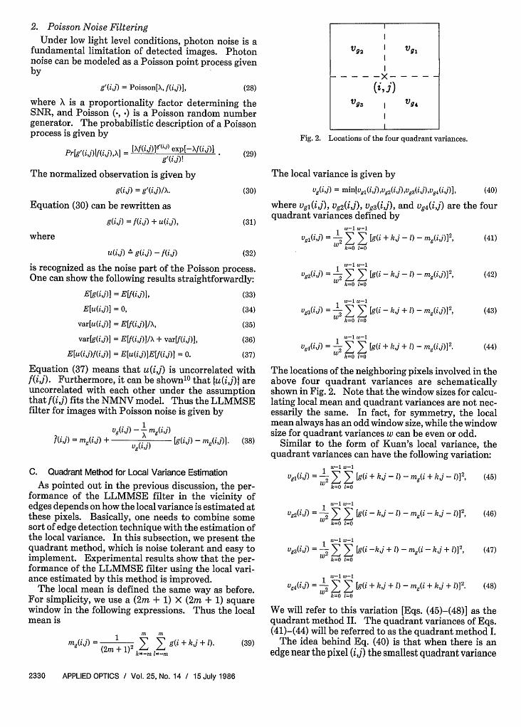
vg(ij) = min[vg1(ij),Vg2(ij),Vg(ij),Vg 4(ij)], (40)

where vgi(ij), Vg2(iI), Vg3(ij), and vg4(ij) are the fourquadrant variances defined by

1w-1 w-12

Vgi(iI) = I I [g(i + kj - 1) - mg(ij)]2,k=0 1=0

(41)

is recognized as the noise part of the Poisson process.One can show the following results straightforwardly:

E[g(ij)] = E[f(ij)],

E[u(ij)] = 0,

var[u(ij)] = E(ij)]IX,

var[g(ij)] = EVf(ij)]/X + varVf(ij)],

E[u(ij)f(ij)] = E[u(ij)IE[f(ij) = 0.

(33)

(34)

(35)

(36)

(37)

1w-1 -1Vg2(Lj) = W2

k=0 1=0

1w-1 -1Vg3(tj) = W2 E

k=0 1=0

1w-1 -1Vg4(,j) = 1 I

k=0 1=0

[g(i - k,j - 1) - mg(ij)]2,

[g(i - k,j + 1) - g(ij)12,

[g(i + kj + 1) - g(ij)]2.

Equation (37) means that u(i,]) is uncorrelated withf(ij). Furthermore, it can be shown'0 that u(ij)} areuncorrelated with each other under the assumptionthat f(ij) fits the NMNV model. Thus the LLMMSEfilter for images with Poisson noise is given by

Vg(i,) --- mg(ij)A(ij) = m,(ij) + X A [g(ij) - mg(ij)]. (38)

Vg(ii)

The locations of the neighboring pixels involved in theabove four quadrant variances are schematicallyshown in Fig. 2. Note that the window sizes for calcu-lating local mean and quadrant variances are not nec-essarily the same. In fact, for symmetry, the localmean always has an odd window size, while the windowsize for quadrant variances w can be even or odd.

Similar to the form of Kuan's local variance, thequadrant variances can have the following variation:

C. Quadrant Method for Local Variance Estimation

As pointed out in the previous discussion, the per-formance of the LLMMSE filter in the vicinity ofedges depends on how the local variance is estimated atthese pixels. Basically, one needs to combine somesort of edge detection technique with the estimation ofthe local variance. In this subsection, we present thequadrant method, which is noise tolerant and easy toimplement. Experimental results show that the per-formance of the LLMMSE filter using the local vari-ance estimated by this method is improved.

The local mean is defined the same way as before.For simplicity, we use a (2m + 1) X (2m + 1) squarewindow in the following expressions. Thus the localmean is

m m

(2m +l ,llEt

Iw-1 -1

Vgi(iJ) = 2

k=0 1=0

Iw-1 -1

Vg2(Lj) = 2 1 E

k=0 1=0

Iw-1 -1

Vg3(ij) 1I2 k=0 1=0

1w-1 -1

Vg4(Lj) = 2 1 E

k=0 1=0

[g(i + k,j - 1) - mg(i + k,j - 1)]2,

[g(i - k,j - 1) - mg(i -k,j - 1)]2,

[g(i -k,j + I) - mg(i - k,j + 1)]2,

[g(i + k,j + 1) - mg(i + khj + 1)]2.

(45)

(46)

(47)

(48)

We will refer to this variation [Eqs. (45)-(48)] as thequadrant method II. The quadrant variances of Eqs.(41)-(44) will be referred to as the quadrant method I.

The idea behind Eq. (40) is that when there is anedge near the pixel (ij) the smallest quadrant variance


(42)

(43)

(44)

has the best chance of being the most representativestatistic over those neighboring pixels around (ij) thatdo not appear across the edge.

The noise sensitivity is kept to a minimum by theeffect of averaging over the w X w window in Eqs. (41)-(48). As far as the noise is concerned, the window sizefor calculating quadrant variances should be chosen aslarge as possible. However, when the window in-creases, the chance that it contains more edges in-creases. Therefore, the appropriate window size willdepend on the complexity of the picture being pro-cessed.

Another problem of this method is the computation-al load and inefficiency. After the smallest quadrantvariance is chosen as the local variance, the other threequantities are useless and discarded. It is easy to seethat the principal computational burden of theLLMMSE filter is in the calculation of the local vari-ances. For quadrant method II, the squared differ-ence between the observation and its local mean can becomputed before the local variance is determined sothat only a summation over the window in Eqs. (45)-(48) is needed to calculate the quadrant variances. Ifwe perform the division by w2, which is part of Eqs.(41)-(48), in Eq. (40) instead, the total number ofoperations for the N2 local variances is 2N2 multiplica-tions and (4w2-3)N2 additions with method II and (4w2

+ 1)N2 multiplications and (8w2 - 4)N2 additions withmethod I.

If we use the quadrant method I [Eqs. (40)-(44)]straightforwardly for each pixel, it will take about fourtimes the computational load compared to the meth-ods simply using Eq. (10). The trick suggested by Leefor the refinement of the local tatistics15 should beborrowed here: the quadrant method I is used only forthose pixels that have local variances calculated by Eq.(10) or (20) exceeding some preset threshold value,which indicates approximately that there are edgesaround the pixels under consideration.

D. Chan-Lim's Work

Chan and Lim12 presented a 1-D approach to theproblem of image restoration. The basic structure isstill the LLMMSE filter described by Eq. (8). Thereare two major differences from Lee's and Kuan's work:

(1) They used 1-D windows to calculate the localstatistics.

(2) Cascaded or repeated LLMMSE filters are used.The cascaded filters use local statistics over 1-D

windows of four different directions, i.e., 0, 45, 90, and1350, respectively. Consider the 0 or horizontal win-dow as an example. The local mean is calculated from

mg(iJ) = 1 l1 g(i + kj). (49)k=-m

The local variance ism

vg(i,) = 2m+ 1 1 [g(i + kj) - mg(ij)12. (50)k-m

The idea behind the cascaded 1-D filters is that asharp edge whose direction is inclined at a large angle

to the filtering direction remains practically intact,while the noise at the edge is removed by one of thefilters oriented closest to the direction of the edge.

1. Noise UpdatingWhen the first filtered output is generated, the noise

variance must be updated so that the second filter canapply to the output of the first filter. If hl(k;ij) repre-sents the unit sample response of the first filter at (ij),the updated noise variance can be estimated by

i+mVui(ij) = I h2(k;ij)v(kj).

k=i-m(51)

Unfortunately, since the LLMMSE filter is not linear,the unit sample response is not clearly defined. Theresponse hl(k;ij) is not given explicitly in the paper.'2An explicit noise updating formula will be derived inthe next section.

E. 1-D Quad-Window Method for Local VarianceEstimation

The 1-D approach proposed by Chan and Lim12improves to a great extent the performance of theLLMMSE filter in both the flat regions and edge loca-tions of the image. It is interesting to see whether theimprovement is really made by the 1-D local statisticsor the filter-cascading structure.

The cascading structure is the subject of the nextsection. In this section, we present the 1-D quad-window method, which estimates the local variancefrom four 1-D local windows in the same fashion as thequadrant method presented earlier. The 2-D localmean, as defined earlier, is repeated here for complete-ness:

mg,(iij) = 1 > g(i +k + 1).(2m+ 1)2 k-m l=-m

The local variance is given by

Vg(tj) = min[Vgl(ij),Vg2(ij),Vg2 (ij),Vg4(ij)],

(52)

(53)

where vgl(ij), Vg2(ij), Vg3(ij), and Vg4(ij) are the foursample variances of 1-D quad-windows oriented in 0,450, 900, and 1350, respectively, defined as follows:

vgi(Lj) = 2w+ 1 1 [g(i + k,j) -mg(i,j)12,

k=-w

Vg2(iJ) = 2w + 1 1 [g(i + k,j - k) - mg(ij)]2 ,k=-w

V93(i0 = Y [g(ij + k) - m(ij)]',k=-w

Vg4(0,I) = 2w + 1 1 [g(i + k,j + k) - g(ij)]2.k=-w

(54)

(55)

(56)

(57)

This will be called the 1-D quad-window method I.Similar to the variation of Kuan's local variance, the 1-D quad-window local variances can also be measuredby


vg(ij) 2+ 1 [g(i + ki)-m 5(i + kj)]2,k=-w

wVg2(3j) = 2w + 1 [g(i + k -k)- mg(i + k - k)]2,

k=-w

V3(ij) = 2 + [g(iij + k) - m(iij + k)] ,k=-w

fA U(I-C Cg-l+ CUC;-L)f,(58)

(66)

(67)U1 (I-CC'l + CuCg;'L)u.

(59)

(60)

w

Vg4(i; = 2w+ 1 E [g(i + k,j +k) -mg(i +k,j +k)]2. (61)k=-w

This will be called the 1-D quad-window method II.As noted before, method II needs less computationthan method I.

IV. Noise Updating Repeated Wiener Filter

In this section, we present the cascaded LLMMSEfilter using 2-D or 1-D local windows. It is called thenoise variance updating repeated Wiener filter, whichborrows the cascading idea directly from Chan andLim.12 One will see that the resulting restoration of a2-D NURW filter has almost the same or even betterMSE improvement compared with a 1-D NURW fil-ter, which is similar to the 1-D algorithm proposed inRef. 12. Before implementing the NURW filter, wemust derive the noise updating formula for the Wienerfilter, which is not given explicitly in Ref. 12.

A. Noise Variance Updating for the Wiener Filter

Consider the observation

g(ij) = f(ij) + u(ij), (62)

where u(ij) is the noise which is uncorrelated with thesignal and has a diagonal covariance matrix. Notethat Eq. (62) can represent not only the additive noisedegradation but also the multiplicative noise degrada-tion [Eq. (22)] and the Poisson noise degradation [Eq.(31)]. Thus what is derived in this subsection appliesto all of these three kinds of noise degradation.

1. 2-D Local Window CaseThe 2-D local mean of g(ij) is

mg (2m + 1)2 g(i+kj+ 1), (63)2m12 k=-m 1=-rn

where a square window is assumed for simplicity. Inlexicographic vector representation, Eq. (63) is repre-sented by

mg = Lg, (64)

where L is the corresponding matrix.the Wiener filter is given by

The output of

Note that because L is not diagonal, the covariancematrix of ul is not diagonal in general. The spatialvariable representation of Eq. (67) is

ul(ij) = 1- I u(i j)

+ i) (2m + 1) 3 u(i + kj +1)

- V(ij) V(im j 1 1L " (i j v(ij) l+1 U(j)Vg(iJ) Vg(i,1) (2m + 1)2

m m

[Vu(ij) 1 1] u(i + k,j + 1).Evg(iJ) (2mn +10 ,=-rn(68)

Because [u(i + kj + l)]kj= m are uncorrelated witheach other, the updated variance of ul(ij) is given by

V~i(i[j) = e -!(i) vj(ij) 1+ 12Vg(ij) V'(ij) (m+12

m m

+ Vu(ii) 1 2 3 L Vg(i j) (2m + 1)2] m V,(i + k,j + 1),

Mkl) 7' (0,0)

(69)

where vu,(ij) is the variance of the original noise u(ij).In the above, we use the fact that

var(aX + bY) = a 2 var(X) + b2 var(Y),

where a and b are constants and X and Y are twouncorrelated random variables. Note that althoughthe local variance vg(ij), which is a statistic of therandom field g(ij), is a random field, we approximateit as a constant in the above derivation for simplicity.

When the filter is repeated, the updated noise is nolonger uncorrelated. However, one can neglect thecorrelation and approximate the covariance matrix oful by a diagonal one with the diagonal elements calcu-lated from Eq. (69). Thus, as the filter is furthercascaded, Eq. (69) can be used to approximate thefurther updated noise variance.

2. 1-D Local Window CaseFor example, consider the horizontal 1-D local win-

dow. The local mean is

91 = Mf + CfgC 1(g-mg)= Lg + (Cg -C 1)C;'(g - Lg)

= (I- + 1, -CuCL)gf + U,

where

mmg(i,,) = 2 I+ g(i +ki).

k=-m

(70)

(65) Following the same procedure as above, we get thenoise updating formula for the horizontal 1-D windowas follows:


V., 1v(ij)+ V (ij) 1 1V(ij)' I V 1 1(iij

V(ij) 1 12 v, ( k) (1+Vg(iI) 2m + k=-M V( +j) (71)

k3#0

The updating formulas for 1-D windows of otherdirections are similar to the above expression. Specif-ically, the term v,(i + kj) in the summation of Eq. (71)is substituted by v>(i + k,j - k), vu(ij + k), and v>(i +kj + k) for the 450, 90°, and 135° 1-D windows, respec-tively. The local mean, Eq. (70), is adjusted accord-ingly in the same fashion.

B. Algorithm for the NURW Filter

Having derived the noise updating formula, we cancascade the LLMMSE or Wiener filters with the localstatistics calculated from 1-D windows of differentorientations as presented in Ref. 12. Note that al-though the repeated 1-D algorithms are the same forthat in Ref. 12 and that used in this paper, the updat-ing formula given in Ref. 12 [Eq. (51)] is different fromEq. (71). To distinguish them, we will refer to thefilter using Eq. (71) for updating as a 1-D NURW filter.One can also use the quadrant local variances as theparameters of the filters and cascade them instead ofonly using the smallest one.

Another possible way is to repeat the filters withdecreasing 2-D local window sizes so that the noise atthe edges left by the first filter can be smoothed out bythe succeeding filters without blurring the edges tooseverely. This is called the 2-D noise variance updat-ing repeated Wiener (NURW) filter. summarized in thefollowing algorithm.

1 Algorithm for the 2-D NURWFilter(1) Choose the number of iterations and the window

size for each iteration.(2) Input the observation [g(ij)].(3) Calculate the local mean [Eq. (9)] and local vari-

ance [Eq. (10) or 20)] of the observation.(4) Calculate the noise variance vu(ij): Eq. (24) for

multiplicative noise, Eq. (35) for Poisson noise.(5) Calculate the LLMMSE filter: Eq. (13) for ad-

ditive noise, Eq. (27) for multiplicative noise, and Eq.(38) for Poisson noise.

(6) If the number of iterations is achieved, stop.(7) For another iteration, update the noise variance

by Eq. (69).(8) Find the local mean [Eq. (9)] and local variance

[Eq. (10) or 20)] of the result of step (5).(9) Go to step (5).Stimulation results of the NURW filter are shown in

the next section.

V. Experimental Results

A. Experimental Noise Generation for Simulation

A sample function of noise is generated with aGaussian random number generator. The mean and

variance of the sample function are measured and usedto normalize the sample to have mean 0 and desiredvariance a'. This normalized sample function is usedin the simulation for additive and multiplicative noisedegradation.

For Poisson noise degradation, the simulation isgenerated from a Poisson random number generatorpixel by pixel independently. No normalization isperformed for the Poisson noise degradation.

B. Additive Noise Restoration

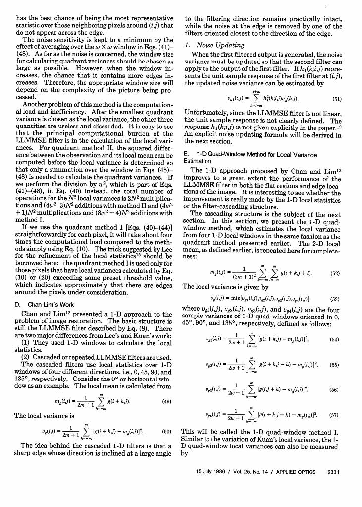
The simulation results for signal-independent addi-tive noise are shown in Figs. 3-6. The original girlimage is shown in Fig. 3(a). The sample mean of thisimage is 98.6. Its sample variance is 2826.0. Figures3(b), 4(a), 5(a), and 6(a) are the degraded image with asignal-independent additive white noise of variance750. The theoretical MSE should be 750. After eight-bit rounding, the calculated MSE is 702.684. In thefollowing, when calculating the MSE improvement, wewill use this calculated value. In restoration and forcalculating SNR, we assume the noise variance is 750.Thus the calculated SNR in terms of variances is -5.76dB. Figure 3(c) is the simple averaging filter outputwhich is the degraded image convolved with a 7 X 7uniform window. It is exactly the local mean used forthe 2-D LLMMSE filter. Figure 3(d) is the output oftwo repeated median filters with cross-shaped win-dows of sizes 7 and 5, respectively. This is given hereas a comparison. The median output may serve as thelocal mean as well.

(a) Original Girl Image

(c) Averaging Filter

(b) Additive Noise, e: = 750

(d) Median Filter

Fig.3. Comparison between an averaging filter and a median filter.


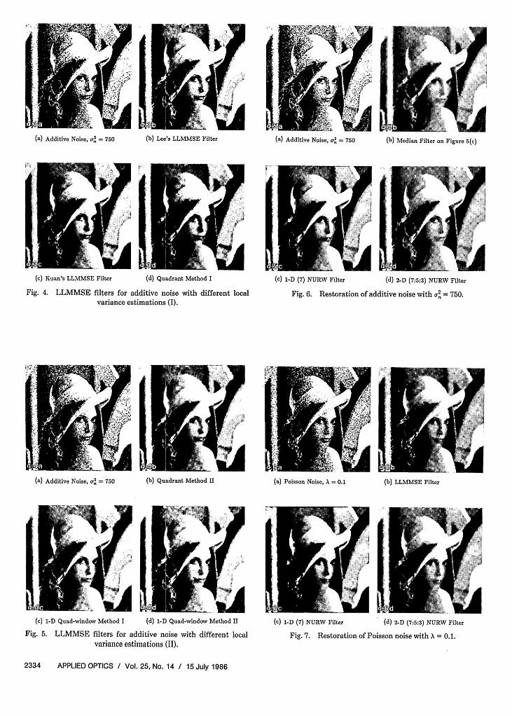
(a) Additive Noise, a' = 750

1

(c) Kuan's LLMMSE Filter (d) Quadrant Method I

Fig. 4. LLMMSE filters for additive noise with different localvariance estimations (I).

(c) 1-D (7) NURW Filter (d) 2-D (7:5:3) NURW Filter

Fig. 6. Restoration of additive noise with a2 = 750.

(a) Additive Noise, a.' = 750 (b) Quadrant Method II (a) Poisson Noise, A = 0.1 (b) LLMMSE Filter

(c) 1-D Quad-window Method I (d) 1-D Quad-window Method II

Fig. 5. LLMMSE filters for additive noise with different localvariance estimations (II).

(c) 1-D (7) NURW Filter (d) 2-D (7:5:3) NURW Filter

Fig. 7. Restoration of Poisson noise with X = 0.1.


I

I

I

Nb Lee's LLMMSE Filter (a) Additive Noise, .' = 750 (b) Median Filter on Figure 5(c)

(b) Multiplicative Noise, e,, = 0.28

(d) Kuan's LLMMSE Filter

Fig. 8. Comparison between Kuan's and Lee's LLMMSE filters formultiplicative noise with a, = 0.28.

(a) The Original Lunar Image

(c) 1-D (7) NURW Filter

(b) Multiplicative Noise, a,, = 0.14

(d) 2-D (5:5:3) NURW Filter

Fig. 9. Restoration of multiplicative noise with a, = 0.14.

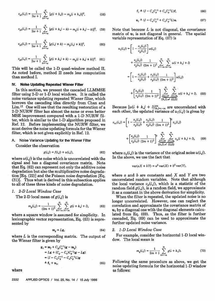
Figure 4(b) is the output of Lee's version of theLLMMSE filter with the local variance calculated byEq. (10). The result of Kuan's version of theLLMMSE filter with local variance calculated by Eq.(20), where the weighting factors are chosen to beuniform, is shown in Fig. 4(c). A 7 X 7 local window isused for both cases. Figure 4(d) is the result of thequadrant method I with m = 3 in Eq. (39) and w = 4 inEqs. (41)-(44).

The result of the quadrant method II with m = 3 inEq. (39) and w = 4 in Eqs. (45)-(48) is shown in Fig.5(b). Figure 5(c) is from the 1-D quad-window meth-od I with m = 3 in Eq. (52) and w = 7 in Eqs. (54)-(57).Figure 5(d) is from the 1-D quad-window method IIwith m = 3 in Eq. (52) and w = 7 in Eqs. (58)-(61).These will be represented as 1-D (7) quad-windowmethods I and II, respectively.

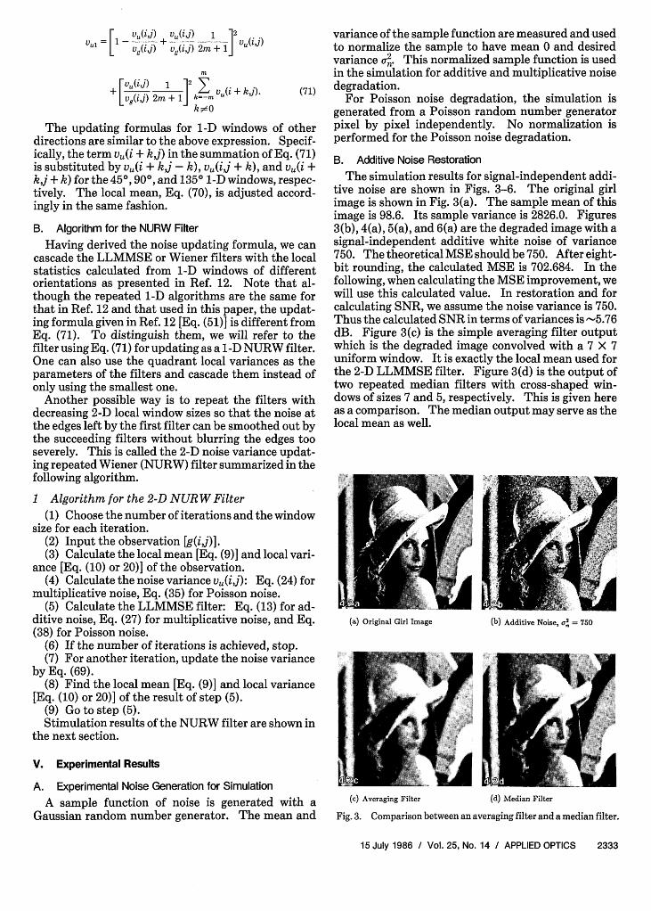
There are white spots across the restored image from1-D (7) quad-window methods I and II. These whitespots, probably coming from too few samples in the 1-D quad-windows used for estimating variance, can beremoved by a median filter. A median filter of a cross-shaped window of size 3 is applied on Fig. 5(c) toremove the white spots. The result is shown in Fig.6(b). Figure 6(c) is from the 1-D NURW filter withlocal size 7. This will be represented by the 1-D (7)NURW filter from now on. Figure 6(d) is from a 2-DNURW filter, which has three iterations with windowsizes of 7 X 7, 5 X 5, and 3 X 3, respectively. Werepresent this filter as a 2-D (7:5:3) NURW filter in thefollowing.

C. Poisson Noise Restoration

The Poisson noise simulation results are shown inFig. 7. Figure 7(a) is the observation corrupted byPoisson noise with parameter X = 0.1 [Eqs. (28)-30)].The calculated SNR is -4.6 dB by using Eqs. (35).Figure 7(b) is from the 2-D LLMMSE filter, Eq. (38),with window size 7 X 7. Equation (10) is used tocalculate the local variance. Figure 7(c) is the 1-DNURW filter output with local size 7. Figure 7(d) isfrom the 2-D (7:5:3) NURW filter.

D. Multiplicative Noise Restoration

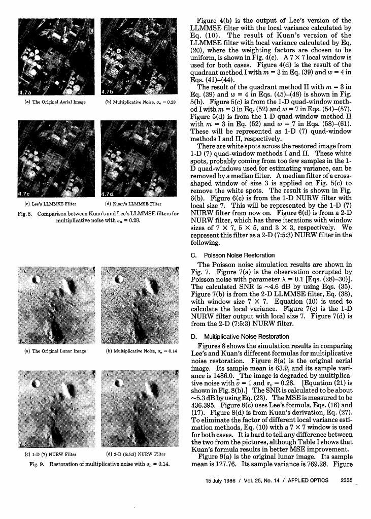
Figures 8 shows the simulation results in comparingLee's and Kuan's different formulas for multiplicativenoise restoration. Figure 8(a) is the original aerialimage. Its sample mean is 63.9, and its sample vari-ance is 1486.0. The image is degraded by multiplica-tive noise with v = 1 and aV = 0.28. [Equation (21) isshown in Fig. 8(b).] The SNR is calculated to be about-5.3 dB by using Eq. (23). The MSE is measured to be436.395. Figure 8(c) uses Lee's formula, Eqs. (16) and(17). Figure 8(d) is from Kuan's derivation, Eq. (27).To eliminate the factor of different local variance esti-mation methods, Eq. (10) with a 7 X 7 window is usedfor both cases. It is hard to tell any difference betweenthe two from the pictures, although Table I shows thatKuan's formula results in better MSE improvement.

Figure 9(a) is the original lunar image. Its samplemean is 127.76. Its sample variance is 769.28. Figure


(a) The Original Aerial Image

(c) Lee's LLMMSE Filter

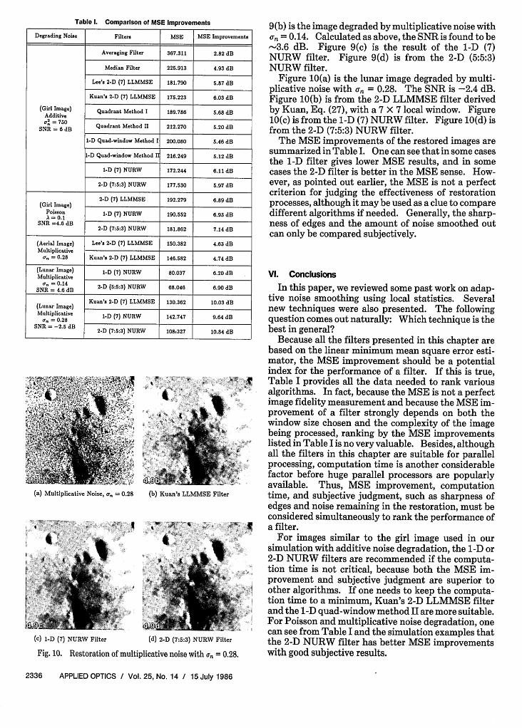
Table I. Comparison of MSE Improvements

Degrading Noise Filters MSE MSE Improvements

Averaging Filter 367.311 2.82 dB

Median Filter 225.913 4.93 dB

Lee's 2-D (7) LLMMSE 181.790 5.87 dB

Kuan's 2-D (7) LLMMSE 175.223 6.03 dB

(Girl Image) Quadrant Method I 189.786 5.68 dBAdditive__________

S2 750 Quadrant Method II 212.270 5.20 dB

1-D Quad-window Method I 200.080 5.46 dB

i-D Quad-window Method I 216.249 5.12 dB

1-D (7) NURW 172.244 6.11 dB

2-D (7:5:3) NURW 177.530 5.97 dB

(Girl Image) 2-D (7) LLMMSE 192.279 6.89 dB

Poisson 1-D (7) NURW 190.552 6.93 dBA = 0.1 ________SNR =4.6 dB

2-D (7:5:3) NURW 181.862 7.14 dB

(Aerial Image) Lee's 2-D (7) LLMMSE 150.382 4.63 dBMultiplicative

a = 0.28 Kuan's 2-D (7) LLMMSE 146.582 4.74 dB

(Lunar Image) 1-D (7) NURW 80.037 6.20 dBMultiplicative

SNR = 6 dB 2-D (5:5:3) NURW 68.046 6.90 dB

Kuan's 2-D (7) LLMMSE 130.362 10.03 dB(Lunar Image)Multiplicative 1-D (7) NURW 142.747 9.64 dBa. = 0.28 __2-_ (:53____10.27 1084_

SNR = 2.5 dB 2-D (7:5:3) NURW 108,327 10.84 dB

(a) Multiplicative Noise, a,, = 0.28

(c) 1-D (7) NURW Filter

(b) Kuan's LLMMSE Filter

(d) 2-D (7:5:3) NURW Filter

Fig. 10. Restoration of multiplicative noise with a,, = 0.28.

9(b) is the image degraded by multiplicative noise withn= 0.14. Calculated as above, the SNR is found to be

-3.6 dB. Figure 9(c) is the result of the 1-D (7)NURW filter. Figure 9(d) is from the 2-D (5:5:3)NURW filter.

Figure 10(a) is the lunar image degraded by multi-plicative noise with r = 0.28. The SNR is -2.4 dB.Figure 10(b) is from the 2-D LLMMSE filter derivedby Kuan, Eq. (27), with a 7 X 7 local window. Figure10(c) is from the 1-D (7) NURW filter. Figure 10(d) isfrom the 2-D (7:5:3) NURW filter.

The MSE improvements of the restored images aresummarized in Table I. One can see that in some casesthe 1-D filter gives lower MSE results, and in somecases the 2-D filter is better in the MSE sense. How-ever, as pointed out earlier, the MSE is not a perfectcriterion for judging the effectiveness of restorationprocesses, although it may be used as a clue to comparedifferent algorithms if needed. Generally, the sharp-ness of edges and the amount of noise smoothed outcan only be compared subjectively.

VI. Conclusions

In this paper, we reviewed some past work on adap-tive noise smoothing using local statistics. Severalnew techniques were also presented. The followingquestion comes out naturally: Which technique is thebest in general?

Because all the filters presented in this chapter arebased on the linear minimum mean square error esti-mator, the MSE improvement should be a potentialindex for the performance of a filter. If this is true,Table I provides all the data needed to rank variousalgorithms. In fact, because the MSE is not a perfectimage fidelity measurement and because the MSE im-provement of a filter strongly depends on both thewindow size chosen and the complexity of the imagebeing processed, ranking by the MSE improvementslisted in Table I is no very valuable. Besides, althoughall the filters in this chapter are suitable for parallelprocessing, computation time is another considerablefactor before huge parallel processors are popularlyavailable. Thus, MSE improvement, computationtime, and subjective judgment, such as sharpness ofedges and noise remaining in the restoration, must beconsidered simultaneously to rank the performance ofa filter.

For images similar to the girl image used in oursimulation with additive noise degradation, the 1-D or2-D NURW filters are recommended if the computa-tion time is not critical, because both the MSE im-provement and subjective judgment are superior toother algorithms. If one needs to keep the computa-tion time to a minimum, Kuan's 2-D LLMMSE filterand the 1-D quad-window method II are more suitable.For Poisson and multiplicative noise degradation, onecan see from Table I and the simulation examples thatthe 2-D NURW filter has better MSE improvementswith good subjective results.


References

1. A. Rosenfeld and A. C. Kak, Digital Picture Processing, Vols. 1

and 2 (Academic, New York, 1982).2. D. S. Lebedev and L. I. Mirkin, "Digital Nonlinear Smoothing of

Images," Institute for Information Transmission Problems,Academy of Sciences, U.S.S.R. (1975), pp. 159-157.

3. V. K. Ingle and J. W. Woods, "Multiple Model Recursive Esti-mation of Images," in Proceedings IEEE, ICASSP 79 (Washing-

ton, DC, Apr. 1979), pp. 642-645.4. B. R. Hunt and T. M. Cannon, "Nonstationary Assumptions for

Gaussian Models of Images," IEEE Trans. System, Man Cyber-net. 6, 876 (1976).

5. B. R. Hunt, "Bayesian Methods in Nonlinear Digital ImageRestoration," IEEE Trans. Comp. C-26, 219 (1977).

6. H. T. Trussell and B. R. Hunt, "Sectioned Methods for Image

Restoration," IEEE Trans. Acoust., Speech Signal ProcessASSP-26, 157 (1978).

7. R. Chellappa and R. L. Kashyap, "Digital Image Restoration

Using Spatial Interaction Models," IEEE Trans. Acoust. SpeechSignal Process. ASSP-30, 461 (1982).

8. D. T. Kuan, A. A. Sawchuk, T. C. Strand, and P. Chavel, "Adap-tive Noise Smoothing Filter for Images with Signal-DependentNoise," IEEE Trans. Pattern Anal. Machine Intell PAMI-7,165(1985).

9. D. T. Kuan, "Nonstationary 2-D Recursive Restoration of Im-

ages with Signal-Dependent Noise with Application to SpeckleReduction," Ph.D. Thesis, U. Southern California, Los Angeles(1982).

10. S-S. Jiang, "Image Restoration and Speckle Suppression Using

the Noise Updating Repeated Wiener Filter," Ph.D. Thesis, U.Southern California, Los Angeles (1986).

11. J. S. Lee, "Digital Image Enhancement and Noise Filtering by

Use of Local Statistics," IEEE Trans. Pattern Anal. MachineIntell. PAMI-2, 165 (1980).

12. P. C. Chan and J. S. Lim, "One-Dimensional Processing forAdaptive Image Restoration, in Proceedings IEEE, ICASSP(San Diego, 1983), pp. 37.3.1-37.3.4.

13. W. K. Pratt, Digital Image Processing (Wiley-Interscience, NewYork, 1978).

14. A. P. Sage and J. L. Melsa, Estimation Theory with Applica-tions to Communications and Control (McGraw-Hill, NewYork, 1971).

15. J. S. Lee, "Refined Noise Filtering Using Local Statistics,"Comput. Graphics Image Process. 15, 380 (1981).

16. G. S. Robinson, "Edge Detection by Compass Gradient Masks,"in Comput. Graphics Image Process. 6, 492 (1977).

0

OSAIAVS

Second Topical

Meeting on

The Microphysics ofSurfaces, Beams,

andAdsorbates

February 16-18, 1987

La Fonda HotelSanta Fe,

New Mexico

Topics To Be CoveredPapers will be solicited in the followingareas:* Bond-specific photochemistry on

surfaces

* Laser photochemistry of adsorbedspecies

* Ion and electron beam inducedreactions on surfaces

* Interfacial chemical kineticsinduced or observed by optical,electron, or ion beam techniques

* Electromagnetism of microstruc-tures and surfaces

* Laser spectroscopy of surfacecollisional processes

* Photochemical etching anddeposition reactions

* Photodesorption

For Information:

Optical Society of America1816 Jefferson PI., NWWashington, D.C. 20036202/223-0920


Documents

Noise updating repeated Wiener filter and other adaptive noise smoothing filters using local image statistics