Nominal Shocks and Real Exchange Rate Fluctuations�

Luciana Juvenaly

Federal Reserve Bank of St. Louis

September 2008

Abstract

I analyze the role of nominal and real shocks on the exchange rate behaviorusing a structural vector autoregressive model (sVAR) for the US vis-à-vis therest of the world. I estimate the contribution of various shocks to explaining themovement of the real dollar exchange rate, imposing two alternative identi�ca-tion strategies based on theoretical restrictions derived from an open economymacro model. Using zero long-run restrictions I �nd that nominal shocks areunimportant to explain real exchange rate �uctuations. I compare this result toan identi�cation strategy based on sign restrictions proposed by Fry and Pagan(2007). The results show that although monetary policy shocks are not the maindrivers of exchange rate �uctuations, they are nevertheless important. The rangefor their short-horizon contribution is 37% to 47%.

Keywords: Exchange Rates, Nominal Shocks, Vector Autoregression, Sign-restrictions.JEL Classi�cation: F31; F41; C30.

�I am grateful to Renee Fry, Gian Maria Milesi-Ferretti and Adrian Pagan for helpful suggestionsand advice at various stages of this paper, and to Giacomo Carboni, Mike Clements, ValentinaCorradi, Sheheryar Malik, Lucio Sarno, Mark P. Taylor, David Wheelock and seminar participantsat the University of Warwick, the City University of New York, Trinity College Dublin, the FederalReserve Bank of St. Louis and the Bank of Spain for comments. This paper presents the author�spersonal opinion and does not necessarily re�ect those of the Federal Reserve Bank of St. Louis orthe US Federal Reserve System.

yCorrespondence address: Research Division, Federal Reserve Bank of St. Louis, P.O. Box 442,St. Louis, MO 63166-0442. Email: luciana.juvenal@stls.frb.org

1

1 Introduction

The explanation of the sources of real exchange rate �uctuations is one of the most

challenging issues in international economics. From a theoretical standpoint, the

literature has focused on the leading role of monetary policy shocks in accounting

for real exchange rate movements. The empirical evidence, however, has not shown

much support that monetary policy shocks are important for real exchange rate

determination. This paper combines a conventional open economy macro model with

recent econometric developments to examine the impact of nominal and real shocks

on the real exchange rate behavior.

A natural starting point for the link between monetary policy and exchange rates

is Dornbusch (1976) model. Dornbusch prediction is that in response to a mone-

tary policy shock the exchange rate would immediately overshoot its long run level

and then adjust gradually. This conclusion follows from two cornerstone arbitrage

conditions: uncovered interest parity (UIP) and purchasing power parity (PPP).

Since Dornbusch�s seminal work, the theoretical literature has mainly concentrated

on the e¤ects of monetary policy shocks (see Obstfeld and Rogo¤, 1995; Beaudry and

Devereux, 1995; Chari et al, 2002). Thus, the belief that monetary policy plays a

dominant role in explaining real exchange rate �uctuations has long been an accepted

fact in economics. Such is the case that Rogo¤ (1996, p. 647) highlights:

�Most explanations of short-term exchange rate volatility point to �nancial factors

such as changes in portfolio preferences, short-term asset price bubbles, and monetary

shocks.�

Although this quote re�ects the �consensus� that nominal shocks are the main

drivers of exchange rate �uctuations, the empirical evidence has not provided much

support to this. In a seminal paper, Clarida and Gali (1994) estimate the relative

contribution of various shocks to real dollar bilateral exchange rates. They �nd that

the contribution of monetary shocks to the variance of the real exchange rate is less

than 3% for the UK and Canadian cases. Eichenbaum and Evans (1995) study the

e¤ects of monetary policy shocks using three di¤erent models. Their results show

that the mean contribution of monetary policy shocks is less than 25%.

Motivated by the previous literature, I concentrate on three issues. Firstly, I

analyze the e¤ects of nominal and real shocks on the real dollar exchange rate. Sec-

ondly, I quantify the importance of nominal vs real shocks for the variance of the real

exchange rate. Thirdly, I evaluate the contribution of each of the shocks to the real

exchange rate behavior. The �rst issue will allow us to study the impact of various

shocks on the real exchange rate and to determine if the e¤ects of monetary policy

2

are consistent with Dornbusch�s overshooting. The second one addresses the question

of whether monetary policy explains a large share of exchange rate �uctuations, as

would be expected from theory. The last one will allow us to link the sources of

exchange rate movements with economic factors and thus will shed some light on the

nature of real exchange rate �uctuations.

The �rst two questions of my analysis have been extensively analyzed in the lit-

erature. For example, Clarida and Gali (1994) and Eichenbaum and Evans (1995)

�nd that the exchange rate overshoots its long-run value after a monetary policy

shock but that the peak occurs from one to three years and not on impact as pre-

dicted by Dornbusch (1976). This result, known as delayed overshooting, became a

consensus result in international economics. In a related study, Faust and Rogers

(2003) �nd that the delayed overshooting result is sensitive to dubious assumptions

of conventional estimation methods. In particular, when simultaneity is allowed be-

tween �nancial market variables (interest rates and exchange rates), they �nd that

overshooting is nearly immediate. In line with Faust and Rogers (2003), Scholl and

Uhlig (2006) show that the exchange rate overshooting takes place much quicker than

the three years horizon found in Eichenbaum and Evans (1995). The literature has

not given a clear cut answer about the proportion of exchange rate variability ex-

plained by monetary policy shocks. In fact, results vary considerably depending on

the countries under consideration and the identi�cation strategy.

The empirical work cited above builds on the use of a structural VAR method

to identify monetary policy shocks. The identi�cation strategy employed varies from

study to study and the ones relying on conventional estimation techniques are subject

to some criticism. Those using zero short-run restrictions (Eichenbaum and Evans,

1995) identify shocks of interest based on some arbitrary assumptions which may

be di¢ cult to reconcile with a broad range of theoretical models. For example, the

assumption of zero contemporaneous impact of a monetary policy shock on output

is in contrast with some general equilibrium models (see Canova and Pina, 1999).

Although long-run restrictions are often better justi�ed by economic theory, there

seem to be cases in which substantial distortions can arise due to the presence of a

small sample bias (Faust and Leeper, 1997) or a lag-truncation bias (Chari, Kehoe

and McGrattan, 2007).

The empirical work based around the use of sign restrictions such as Faust and

Rogers (2003) and Scholl and Uhlig (2006) are not subject to the criticism of relying

on arbitrary assumptions given that the identifying assumptions are derived from a

theoretical model. In these studies the identi�cation of the shock of interest - a mon-

etary policy shock - is achieved by imposing sign restrictions on impulse responses

3

while being agnostic about the response of the key variable of interest - in this case

the exchange rate. However, as shown by Paustian (2007) this procedure does not

guarantee that the identi�cation of structural shocks is exact because there are mul-

tiple matrices de�ning the linear mapping from orthogonal structural shocks to VAR

residuals.

As a way to obtain more precise estimates of impulse responses, the sign restric-

tions method can be generalized to identify more than one shock. In this case the

estimation is more precise because the range of reasonable impulse responses is nar-

rowed down. To see this, note that when only one shock is identi�ed, for example,

a monetary policy shock, impulse responses that satisfy the sign restrictions of the

monetary policy shock are accepted even if the responses to other shocks are unrea-

sonable. This issue is avoided when more than one shock is identi�ed because only

the set of impulse responses that jointly satisfy all sign restrictions for all shocks are

accepted. An example of this method is illustrated in Farrant and Peersman (2006),

who analyze whether the real exchange rate is a shock absorber or a source of shocks

for a series of dollar bilateral exchange rates using a sign restrictions method that

identi�es various shocks of interest. They �nd an important role of the real exchange

rate as a shock absorber, mainly of demand shocks. In a related study, Fry and

Pagan (2007) highlight some conceptual problems of this method, which result from

the multiplicity of impulse vectors and suggest a rule to pin down unique impulse

responses using sign restrictions.

In an attempt to overcome the limitations previously mentioned, this paper builds

on Farrant and Peersman (2006) but re�nes the estimation strategy by applying the

method developed by Fry and Pagan (2007). The results based on this approach

yield an important addition to the literature. I provide evidence that monetary

policy shocks are a relevant driver of the real exchange rate. This reconciles the focus

of the theoretical literature on monetary policy with the empirical evidence.

More precisely, I estimate the standard 3 variable VAR of Clarida and Gali (1994)

composed of relative output, relative prices and the real exchange rate and identify

supply, demand and nominal shocks. In the paper I will refer interchangeably to

nominal and monetary shocks. Based on the theoretical restrictions derived from the

Clarida-Gali model, I use two alternative identi�cation strategies. The �rst one is

based on the Blanchard and Quah (1989) method and is derived from the long-run

dynamics of the model. The second one employs sign-restrictions derived from the

theoretical short-run predictions of the model.

Using long-run restrictions I get the conventional empirical �nding that nominal

shocks are unimportant to explain real exchange rate �uctuations. The evidence

4

I present in this paper indicates that, in contrast to this result, when using sign

restrictions monetary (or nominal) shocks are an important driver of exchange rate

movements at short horizons. I �nd that at a 4 quarters horizon, the contribution

of monetary policy shocks is 47%. Their relative importance is reduced at longer

horizons. Indeed, at a horizon of 20 quarters only 20% of the variation of the real

exchange rate is explained by monetary policy shocks. Our results di¤er from what

is typically found in the literature.1

I then examine the sensitivity of my results to the use of alternative sign re-

strictions, to a sub-sample analysis, to a di¤erent exchange rate measure and to

an extended model. Overall, I �nd that the results are robust to these alternative

speci�cations. I also examine the robustness of my results to an extended model

where the identi�cation strategy is based on zero short-run restrictions. When us-

ing this method monetary policy shocks explain only 10% of the movement of the

real exchange rate at all horizons. Interestingly, this identi�cation strategy yields a

signi�cant �puzzle�, thus casting doubt on its validity.

The remainder of the paper is organized as follows. Section 2 outlines the Clarida

and Gali (1994) model. Section 3 describes the data and also presents unit root

and cointegration tests. The results using the long-run identi�cation strategy are

presented in Section 4. Section 5 contains the empirical methodology based on a

structural VAR framework with sign restrictions. The results of the baseline model

are presented in Section 6 while I report a battery of robustness tests in Section 7.

Section 8 concludes.

2 Theoretical model

I estimate a structural VAR using two alternative identi�cation strategies based on

theoretical restrictions derived from the Clarida-Gali model. The �rst identi�cation

strategy is the same as the one used by Clarida-Gali and relies on imposing zero

long-run restrictions based on the long-run dynamics of the model. The second one

employs sign-restrictions derived from the theoretical short-run predictions of the

model.

The Clarida-Gali model is a stochastic version of the two-country rational expec-

tations model by Obstfeld (1985). The model captures the short-run dynamics of

the Mundell-Fleming-Dornbusch approach when prices adjust sluggishly to demand,

supply and monetary shocks as well as the long-run dynamics, when the economy is

in equilibrium and prices fully adjust to all shocks. The following set of equations1An important exception is Rogers (1999), where he presents evidence that monetary policy shocks

are generally important for real exchange rate movements.

5

describe the model. All variables are in logs except interest rates and represent home

(US) relative to foreign (rest of the world) levels.

ydt = dt + � (st � pt)� � [it � Et (pt+1 � pt)] (1)

pt = (1� ')Et�1pet + 'pet (2)

mst � pt = yt � �it (3)

it = Et (st+1 � st) (4)

Equation (1) is an open-economy IS equation, in which relative output demand�ydt�depends positively on a relative demand shock (dt) and on the real exchange rate

(qt = st � pt), and is decreasing in the real interest rate di¤erential. In this modeldt captures any shock to home absorption relative to foreign absorption (e.g. �scal

shocks). Equation (2) is a price setting equation in which the relative price level in

period t (pt) is an average of the market-clearing price in t � 1, (Et�1pet ) and theprice that would actually clear the market in time t, (pet ). The parameter ' is a

measure of price sluggishness. When ' = 1 prices are fully �exible and output is

supply determined and when ' = 0 prices are �xed and predetermined one period in

advance. Equation (3) is an LM equation in which real money balances are increasing

in relative output (yt) and decreasing in the relative interest rate (it). Equation (4)

is an interest parity condition in which st denotes the nominal exchange rate.

In the Clarida and Gali (1994) model, relative output, relative prices and the

real exchange rate are driven by three shocks: a relative supply shock, a relative

demand shock and a relative monetary shock.2 Both yst and mt are assumed to

follow a random walk process and dt is characterized by a transitory and permanent

component:

yst = yst�1 + �st (5)

dt = dt�1 + �dt � �dt�1 (6)

mt = mt�1 + �mt (7)

The model can be solved for the long-run �exible-price equilibrium, described by

the following equations:3

2Note that the monetary shock re�ects both shocks to relative monety supply and to relativemoney demand.

3For details on the derivation of the model see Clarida and Gali (1994).

6

yet = yst (8)

qet = (yst � dt) =� + [� (� + �)]�1 � "dt (9)

pet = mt � yst + � (1 + �)�1 (� + �)�1 "dt (10)

Thus, in the long run, only supply shocks lead to increases in the level of relative

output; supply and demand shocks have an impact in the long-run level of the real

exchange rate; and the three shocks have an impact on relative prices in the long

run. The theoretical long-run predictions of the model are summarized in Table 1,

where � denotes that the shocks have an impact on the variables in the long-run and0 implies that they do not.

Table 1. Theoretical PredictionsLong-run predictions Short-run predictions

Shock y � y� q p� p� y � y� q p� p�

Supply � � � + � �Demand 0 � � + + +Nominal 0 0 � + � +

The zero long-run restrictions are used by Clarida and Gali (1994) to identify

supply, demand and nominal shocks. I will replicate their identi�cation strategy but

I will also use the theoretical short-run predictions of their model to estimate the

impact of the shocks of interest employing a method based on sign restrictions.

Solving the system for the case of a short-run open economy equilibrium with

sluggish price adjustment, we obtain:

pt = pet � (1� ')��mt � �st + � "dt

�(11)

qt = qet + � (1� ')��mt � �st + � "dt

�(12)

yt = yst + (� + �) � (1� ')��mt � "st + "dt

�(13)

where � � �(1 + �)�1(� + �)�1, � � (1 + �) (�+ � + �)�1 :Equations (11), (12) and (13) describe the evolution of relative price levels, the real

exchange rate and relative output in the short run, when the economy is characterized

by a certain degree of price sluggishness, such that 1 < ' < 0.

The predictions of the model are the following. In response to a positive monetary

shock, relative output and relative prices increase and the exchange rate depreciates.

7

A demand shock leads to an increase in output and relative prices and an appreciation

of the real exchange rate. In response to a supply shock relative output increases,

relative prices decrease and the real exchange rate depreciates. These restrictions,

summarized as well in Table 1 above, refer to the short-run impact of the three shocks

on the variables of interest.4 I will incorporate these short-run sign restrictions into

an empirical model and identify the shocks of interest in an alternative way with

respect to the original Clarida-Gali approach.

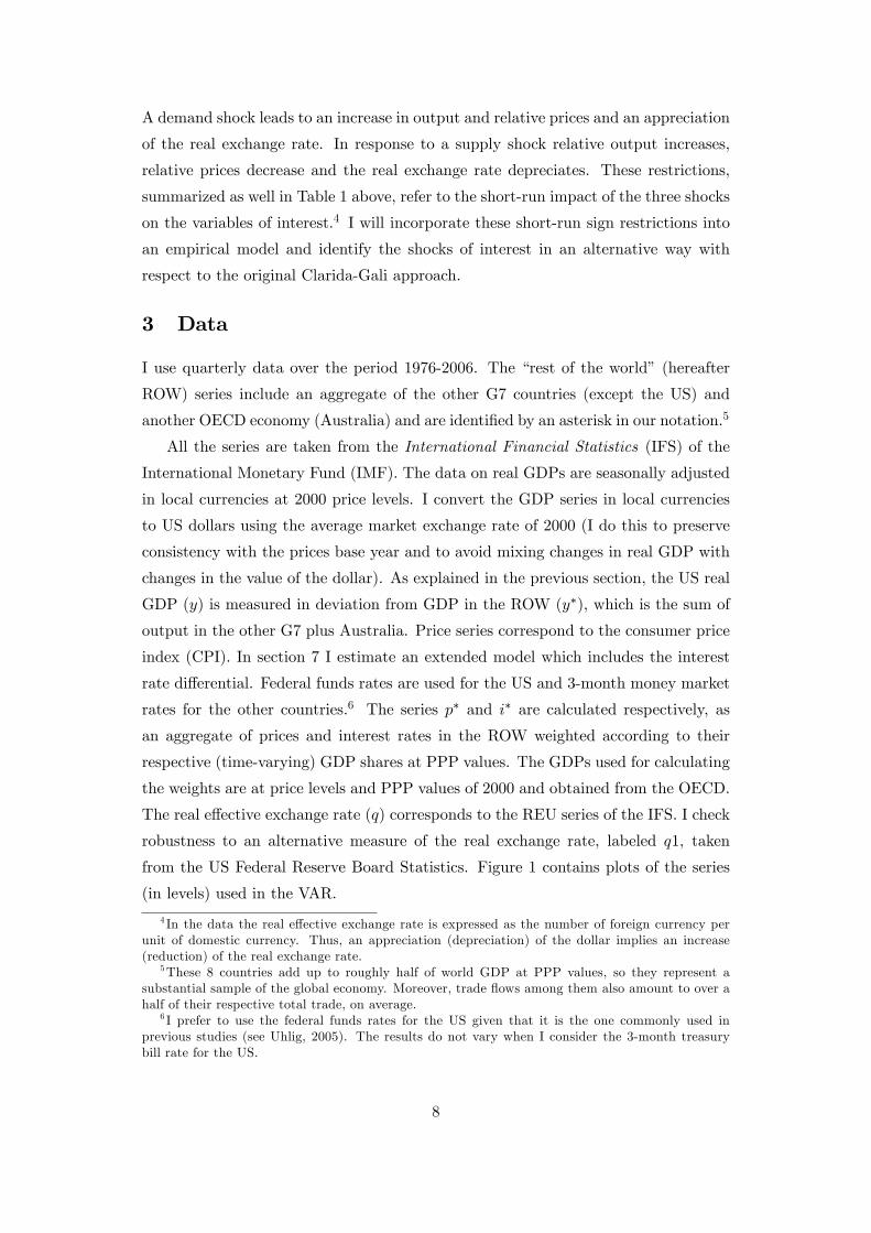
3 Data

I use quarterly data over the period 1976-2006. The �rest of the world� (hereafter

ROW) series include an aggregate of the other G7 countries (except the US) and

another OECD economy (Australia) and are identi�ed by an asterisk in our notation.5

All the series are taken from the International Financial Statistics (IFS) of the

International Monetary Fund (IMF). The data on real GDPs are seasonally adjusted

in local currencies at 2000 price levels. I convert the GDP series in local currencies

to US dollars using the average market exchange rate of 2000 (I do this to preserve

consistency with the prices base year and to avoid mixing changes in real GDP with

changes in the value of the dollar). As explained in the previous section, the US real

GDP (y) is measured in deviation from GDP in the ROW (y�), which is the sum of

output in the other G7 plus Australia. Price series correspond to the consumer price

index (CPI). In section 7 I estimate an extended model which includes the interest

rate di¤erential. Federal funds rates are used for the US and 3-month money market

rates for the other countries.6 The series p� and i� are calculated respectively, as

an aggregate of prices and interest rates in the ROW weighted according to their

respective (time-varying) GDP shares at PPP values. The GDPs used for calculating

the weights are at price levels and PPP values of 2000 and obtained from the OECD.

The real e¤ective exchange rate (q) corresponds to the REU series of the IFS. I check

robustness to an alternative measure of the real exchange rate, labeled q1, taken

from the US Federal Reserve Board Statistics. Figure 1 contains plots of the series

(in levels) used in the VAR.

4 In the data the real e¤ective exchange rate is expressed as the number of foreign currency perunit of domestic currency. Thus, an appreciation (depreciation) of the dollar implies an increase(reduction) of the real exchange rate.

5These 8 countries add up to roughly half of world GDP at PPP values, so they represent asubstantial sample of the global economy. Moreover, trade �ows among them also amount to over ahalf of their respective total trade, on average.

6 I prefer to use the federal funds rates for the US given that it is the one commonly used inprevious studies (see Uhlig, 2005). The results do not vary when I consider the 3-month treasurybill rate for the US.

8

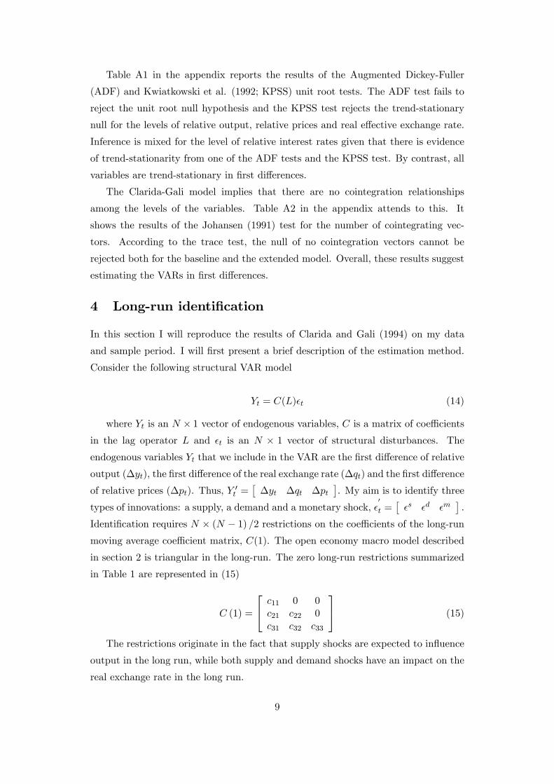
Table A1 in the appendix reports the results of the Augmented Dickey-Fuller

(ADF) and Kwiatkowski et al. (1992; KPSS) unit root tests. The ADF test fails to

reject the unit root null hypothesis and the KPSS test rejects the trend-stationary

null for the levels of relative output, relative prices and real e¤ective exchange rate.

Inference is mixed for the level of relative interest rates given that there is evidence

of trend-stationarity from one of the ADF tests and the KPSS test. By contrast, all

variables are trend-stationary in �rst di¤erences.

The Clarida-Gali model implies that there are no cointegration relationships

among the levels of the variables. Table A2 in the appendix attends to this. It

shows the results of the Johansen (1991) test for the number of cointegrating vec-

tors. According to the trace test, the null of no cointegration vectors cannot be

rejected both for the baseline and the extended model. Overall, these results suggest

estimating the VARs in �rst di¤erences.

4 Long-run identi�cation

In this section I will reproduce the results of Clarida and Gali (1994) on my data

and sample period. I will �rst present a brief description of the estimation method.

Consider the following structural VAR model

Yt = C(L)�t (14)

where Yt is an N � 1 vector of endogenous variables, C is a matrix of coe¢ cientsin the lag operator L and �t is an N � 1 vector of structural disturbances. Theendogenous variables Yt that we include in the VAR are the �rst di¤erence of relative

output (�yt), the �rst di¤erence of the real exchange rate (�qt) and the �rst di¤erence

of relative prices (�pt). Thus, Y 0t =��yt �qt �pt

�. My aim is to identify three

types of innovations: a supply, a demand and a monetary shock, �0

t =��s �d �m

�:

Identi�cation requires N � (N � 1) =2 restrictions on the coe¢ cients of the long-runmoving average coe¢ cient matrix, C(1). The open economy macro model described

in section 2 is triangular in the long-run. The zero long-run restrictions summarized

in Table 1 are represented in (15)

C (1) =

24 c11 0 0c21 c22 0c31 c32 c33

35 (15)

The restrictions originate in the fact that supply shocks are expected to in�uence

output in the long run, while both supply and demand shocks have an impact on the

real exchange rate in the long run.

9

The restriction c12 = 0 implies that demand shocks, �d, have no e¤ect on output in

the long run. The restriction that nominal shocks have no impact on relative output

and the real exchange rate in the long run justi�es that c13 = 0 and c23 = 0. Note

that by only imposing zero long-run restrictions we leave the short-run dynamics of

the model unrestricted. Thus, we can assess whether the shocks that this approach

identi�es as due to supply, demand and money are consistent with the short-run

dynamics of the model presented in section 2.

Figure 2 shows the impulse responses to a supply, demand and nominal shock to-

gether with the 16th and 84th percentiles error bands calculated using Monte Carlo

integration. Consistent with the predictions of the model, a supply shock has a per-

sistent positive e¤ect in relative output and a persistent negative e¤ect on relative

prices. However, after a supply shock the real exchange rate exhibits a temporary

appreciation, which is in contrast with the predictions of the theoretical model. In

line with the theoretical model, demand shocks lead to a temporary increase in rel-

ative output. This result is obtained by construction, because demand shocks are

restricted not to a¤ect relative output in the long run. After a demand shock the real

exchange rate exhibits a persistent appreciation. Finally, a monetary policy shock

has a temporary e¤ect on relative output and a persistent e¤ect on relative prices.

Interestingly, after a monetary shock the real exchange rate overshoots its long-run

value almost immediately (in one quarter). This is in contrast to the popular one to

three years delayed overshooting found in the earlier literature (see Eichenbaum and

Evans, 1995) .

The variance decomposition can be used to assess how much of the variance

of the real exchange rate is given by supply, demand and monetary shocks over

di¤erent forecast horizons. The results, given in Table 2, are in line with the ones

presented in Clarida and Gali (1994). Nominal shocks are unimportant to explain

real exchange rates �uctuations, as demand shocks are the main driver of the real

exchange rate. At a horizon of 4 and 20 quarters, 86% and 93% of the variation

of the real exchange rate is explained by demand shocks, respectively. By contrast,

nominal shocks explain between 1% and 7% of the variance of the real exchange rate

at 4 and 20 quarters, respectively. The results also show that supply shocks play a

minimal role in explaining real exchange rate �uctuations.

10

Table 2. Variance Decomposition of the Real E¤ective Exchange Rate

(Long-run restrictions, Sign restrictions and short-run restrictions)Shocks

Steps Supply Demand Nominal4 quarters CG 0.06 [0.01 ; 0.17] 0.86 [0.71 ; 0.94] 0.07 [0.02 ; 0.15]

SR1 0.03 [0.00 ; 0.11] 0.50 [0.24 ; 0.71] 0.47 [0.23 ; 0.71]SR2 0.02 [0.00 ; 0.11] 0.49 [0.24 ; 0.71] 0.48 [0.23 ; 0.71]

8 quarters CG 0.05 [0.01 ; 0.16] 0.90 [0.78 ; 0.96] 0.03 [0.01 ; 0.08]SR1 0.05 [0.01 ; 0.14] 0.58 [0.31 ; 0.80] 0.37 [0.14 ; 0.61]SR2 0.04 [0.01 ; 0.14] 0.57 [0.31 ; 0.80] 0.38 [0.14 ; 0.61]

12 quarters CG 0.05 [0.01 ; 0.16] 0.92 [0.81 ; 0.97] 0.02 [0.01 ; 0.05]SR1 0.07 [0.01 ; 0.17] 0.65 [0.35 ; 0.84] 0.28 [0.09 ; 0.54]SR2 0.06 [0.01 ; 0.17] 0.66 [0.35 ; 0.84] 0.27 [0.09 ; 0.54]

16 quarters CG 0.05 [0.01 ; 0.16] 0.92 [0.82 ; 0.98] 0.02 [0.00 ; 0.04]SR1 0.08 [0.01 ; 0.19] 0.68 [0.39 ; 0.86] 0.24 [0.07 ; 0.48]SR2 0.07 [0.01 ; 0.19] 0.68 [0.39 ; 0.86] 0.24 [0.07 ; 0.48]

20 quarters CG 0.05 [0.01 ; 0.16] 0.93 [0.83 ; 0.98] 0.01 [0.00 ; 0.03]SR1 0.10 [0.01 ; 0.20] 0.70 [0.42 ; 0.87] 0.20 [0.06 ; 0.44]SR2 0.08 [0.01 ; 0.20] 0.70 [0.42 ; 0.87] 0.22 [0.06 ; 0.44]

Notes: The table shows the percentage of the error variance of the real e¤ective exchangerate due to each shock at 4, 8, 12, 16 and 20 quarter horizons. Lag length is 4. In bracketsare the 16th and 84th percentiles error bands. CG denotes that identi�cation is based on theClarida-Gali approach. SR1 refers to the baseline sign restrictions described in Table 1. SR2denotes the alternative sign restrictions presented in section 7.

5 Identi�cation using short-run sign restrictions

The method based on long-run restrictions described in the previous section is very

appealing because it is often justi�ed by economic theory. However, the technique has

a series of shortcomings. One is that there are cases in which the impulse responses

contradict predictions of the theoretical model. Another is related to the �nding

of Faust and Leeper (1997) who show that substantial distortions can arise due to

small sample biases and measurement errors when using long-run restrictions. In a

related study, Chari, Kehoe and McGrattan (2007) show that sVARs with long-run

restrictions su¤er from a lag-truncation bias. This happens because the available

data requires a VAR with a small number of lags, which is a poor approximation of

the in�nite-order VAR of the observables from the model.

Conventional methods involving zero-short run restrictions, such as the Choleski

decomposition, have also been questioned on various grounds. Firstly, they are usu-

ally derived from some arbitrary assumptions which may be di¢ cult to reconcile with

theoretical models. For example, the assumption of zero contemporaneous impact of

a monetary policy shock on output is in contrast with some general equilibrium mod-

11

els (see Canova and Pina, 1999). Secondly, they sometimes yield counter-intuitive

impulse response functions of key endogenous variables which are not easy to ratio-

nalize on the basis of conventional economic theory. An example is the so called

�price puzzle�, which refers to the increase in prices after a monetary tightening (see

Sims and Zha, 2006; Christiano, Eichenbaum and Evans, 1999; Kim and Roubini,

2000). Thirdly, as noted by Sarno and Thornton (2004), the results are often sensitive

to the ordering of the variables.

In order to overcome the potential problems of the previous methods, I use an

alternative identi�cation procedure based on sign restrictions. Faust (1998), Canova

and de Nicoló (2002) and Uhlig (2005) use sign restrictions to identify one shock, a

monetary policy shock. Since I am interested in identifying a full set of shocks, I

employ a methodology that extends the sign restriction approach to identify more

than one shock. In particular, I apply the method described in Fry and Pagan (2007),

who highlight some conceptual problems arising from the multiplicity of impulse

vectors. Their approach builds on Mountord and Uhlig (2005) and Peersman (2005).

I would like to emphasize that the decision to use the approach of sign restrictions

proposed by Fry and Pagan (2007) does not represent a general criticism of other sign

restrictions methods. Indeed, some authors have proposed the use of identi�cation

schemes that pin down unique impulse responses. Uhlig (2005), for example, proposes

the use of a penalty function.

I am interested in analyzing the impact of demand, supply and nominal shocks

on the real exchange rate avoiding the problems arising from imposing arbitrary

assumptions. Thus, the identi�cation of the shocks is based on the theoretical short-

run predictions of the Clarida-Gali model outlined in section 2. In contrast to what

I did in the previous section, I will now impose restrictions in the short-run and let

the data speak in the long-run.

5.1 VAR model with sign restrictions

Consider the reduced form VAR

Yt = c+B(L)Yt�1 +A�t (16)

where c is an N � 2 matrix of constants and linear trends, Yt is the N � 1 vectorof endogenous variables; B(L) is a matrix polynomial in the lag operator L; �t is an

N � 1 vector of structural innovations. The endogenous variables Yt that we includein the VAR are the same as the ones in the previous section.

My aim is to identify three types of innovations: a supply, a demand and a mon-

12

etary shock, �0

t =��s �d �m

�: I identify these shocks using a sign restriction

approach. Since the shocks are assumed to be orthogonal, so that E[�t�0t] = I, the

variance-covariance matrix of equation (16) is equal to: � = AA0: For any orthogonal

decomposition of A, we can �nd an in�nite number of possible orthogonal decompo-

sition of �, such that � = AQQ0A0, where Q is any orthonormal matrix (QQ0 = I).

A Choleski decomposition, for example, would assume a recursive structure on A so

that A is lower triangular. Another candidate for A is the eigenvalue-eigenvector de-

composition, � = PDP 0 = AA0, where P is a matrix of eigenvectors, D is a diagonal

matrix of eigenvalues and A = PD1=2: This decomposition generates orthonormal

shocks, making the value of P unique for each variance-covariance matrix decompo-

sition without imposing zero restrictions. Following Canova and de Nicoló (2002), I

consider P =N�1Qm=1

NQn=m+1

Qm;n(�), where Qm;n(�) is an orthonormal rotational matrix

of the form:

Qm;n =

2666641 0 ::: 0 00 cos(�) ::: � sin(�) 0::: ::: 1 ::: :::0 sin(�) ::: cos(�) 00 0 ::: 0 1

377775 (17)

where (m,n) indicate that the rows m and n are being rotated by the angle �.

In a 3 variable model we have a 3x3 rotational matrix Q and 3 bivariate rotations.7

The angles � = �1; :::; �3; and the rows m and n are rotated such that

P =

24 cos(�1) � sin(�1) 0sin(�1) cos(�1) 00 0 1

3524 1 0 0cos(�2) � sin(�2)

0 sin(�2) cos(�2)

3524 cos(�3) 0 � sin(�3)0 1 0

sin(�3) 0 cos(�3)

35My estimation strategy follows Fry and Pagan (2007) and Peersman (2005) and

is carried out as follows. Firstly, all possible rotations are produced by varying

the rotation angles �1, �2, �3 in the range [0; �] : For practical purposes, I grid the

interval [0; �] into M points. After estimating the coe¢ cients of the B(L) matrix

using ordinary least squares (OLS), the impulse responses of N variables up to K

horizons can be calculated for the contemporaneous impact matrix, Aj(j = 1; :::;M3)

as follows:

Rj;t+k = [I �B(L)]�1Aj�t (18)

where Rj;t+k is the matrix of impulse responses at horizon k. In order to identify

7 In general terms, we have a total of N(N-1)/2, where N is the number of variables.

13

the shock v of interest, sign restrictions can be imposed on p 5 n variables over thehorizon 0; :::;K in the form:

Rp; vj;t+k 7 0 (19)

The sign restrictions are imposed based on the Clarida-Gali open economy model

as summarized in Table 1 over the time horizon k = 0; :::;K. Details about the

number of periods for which the restrictions hold are given below.

To identify a supply shock, s, I impose that relative output does not decrease,

relative prices do not increase for four quarters (K = 4) and that the real exchange

rate does not appreciate for one quarter (K = 1):8

Ry�y�; s

j;t+k > 0; k = 0; :::; 4

Rp�p�; s

j;t+k 6 0; k = 0; :::; 4

Rq; sj;t+k 6 0; k = 0; 1

The restrictions to identify a demand shock, d, are that relative output and rela-

tive prices do not decrease for four quarters and that the real exchange rate does not

depreciate for one quarter:

Ry�y�; d

j;t+k > 0; k = 0; :::; 4

Rp�p�; d

j;t+k > 0; k = 0; :::; 4

Rq; dj;t+k > 0; k = 0; 1

A monetary policy shock, m, is identi�ed by restricting relative output and rela-

tive prices not to decrease for four quarters and the real exchange rate not to appre-

ciate for one quarter:

Ry�y�; m

j;t+k > 0; k = 0; :::; 4

Rp�p�; m

j;t+k > 0; k = 0; :::; 4

Rq; mj;t+k 6 0; k = 0; 1

Out of all possible rotations I select those that satisfy the sign restrictions of the

impulse responses of the three shocks. Impulse responses are constructed using a

8Changing the values of the number of quarters for which the restrictions are binding has no e¤ecton the conclusions of the results.

14

Monte Carlo experiment. For each Monte Carlo draw, I draw one rotation out of all

possible rotations and check if the imposed restrictions are satis�ed for all shocks.

Solutions that satisfy all the restrictions are kept and the others are discarded. In

practice I repeat this procedure until 1000 draws satisfying the restrictions are found.

5.1.1 Summarizing the information

A common way to present the information is by reporting the median of the impulse

responses based on a certain number of solutions. As noted by Fry and Pagan (2007),

this may not provide a useful measure. Let us consider as an example the responses of

two variables to one shock. Say that �1(i) represents the impulse responses of variable

1 and �2(i) represents the impulse responses of variable 2, where i indexes the values of

�. What is usually presented is med((�1(i)) and med((�2(i)). If �1(i) was monotonic

in �, this would be �1(med(�(i))). Thus, the median of the impulse responses would

be generated by the same model, represented by med(�(i)). Given that there is no

guarantee of monotonicity, the median of the impulse responses will generally be

associated with di¤erent values of �. Thus, the median of the impulse responses will

not come from a single model. This will happen for the impulse responses of all

variables and for all shocks. As a consequence, the shocks identi�ed are no longer

orthogonal to each other. Apart from the fact that the assumption of uncorrelated

shocks is essential to estimate a VAR model, if correlations are non-zero, the variance

decomposition does not exist.9

Fry and Pagan (2007) suggest locating a unique vector of ��s such that the im-

pulses are closest to its median while maintaining the orthogonality condition. This

method works as follows. Impulse responses are calculated based on those that satisfy

the sign restrictions as described above. Given that the impulse responses are not

unit free, they are standardized by subtracting their median and dividing by their

standard deviation. These standardized impulse responses are included in a vector

�i for each value of �i (in the 2 variable case below � is a 4�1 vector as there are 4impulse responses. The choice of � is the one that minimizes the following quantity.

(�i) = �0i�i (20)

Substituting �min into Q(�) will produce a set of orthogonal shocks and the de-

scriptive statistics are computed based on this rotation.

9This problem remains even if only one single shock is identi�ed, as in Uhlig (2005), since thereis nothing that ensures it is uncorrelated with the remaining shocks in the model when consideringthe median of impulse responses.

15

6 Empirical results

6.1 Estimates of the baseline model

I now turn to the empirical �ndings, by presenting the benchmark results from im-

plementing the VAR described in Section 5.

Figure 3 shows the impulse responses of relative output, relative in�ation and the

exchange rate with respect to the three shocks of interest. The impulse responses

suggest that a supply shock leads to a persistent depreciation of the real exchange

rate. More precisely, the US dollar depreciates 0.5% on impact and it continues to

decline until it reaches a depreciation of 1.3% after 9 quarters. In addition, a supply

shock generates a persistent increase in relative output and a persistent decrease in

relative prices.

After a demand shock, there is a persistent rise of around 0.8% in relative output.

By contrast, there is a temporary e¤ect on relative prices, which increase 0.07% on

impact. The real exchange rate appreciates 2% on impact and it continues to rise up

to 3.7% after 9 quarters.

Finally, a monetary policy (or nominal) shock leads to a temporary depreciation

of the US dollar. After an initial depreciation of 2%, the real exchange rate reaches

its minimum value after 3 quarters and then reverts to equilibrium (consistent with

PPP), showing no statistically signi�cant reaction after 10 quarters. This result

supports the delayed overshooting conclusion given that the peak is not immediate as

predicted in Dornbusch (1976). A monetary shock also leads to a temporary positive

e¤ect on relative output (it increases 0.5% on impact and shows no signi�cant reaction

after 6 quarters) and a persistent rise in relative prices, which increase by 1% after 9

quarters.

The long-run predictions of the Clarida-Gali model are satis�ed empirically except

for the impact of a demand shock on relative output. According to the theoretical

model, only supply shocks in�uence the long run level of output. However, the

empirical results show that demand shocks also have a persistent e¤ect on output.

Table 2 compares the variance decomposition of the real exchange rate using

the sign restrictions (SR1) and the Clarida-Gali (CG) methodologies. From Table

2 it is clear that there is a stark di¤erence in the results from both identi�cation

procedures. Using the sign-restrictions method we conclude that a substantial share

of the variation in the real exchange rate is explained by monetary shocks over short

horizons but at long horizons their relative importance is reduced. Indeed, at a 4

quarters horizon the contribution of monetary policy shocks to real exchange rate

�uctuations is 47%. At a horizon of 20 quarters only 20% of the variation of the

16

real exchange rate is explained by monetary policy shocks. By contrast, demand

shocks explain a substantial proportion of the variance of the real exchange rate

both at short and long horizons (50% and 70% at a horizon of 4 quarters and 20

quarters respectively). The results also show that supply shocks play a minimal role

in explaining real exchange rate �uctuations. In particular, I �nd that supply shocks

explain 3%, 7% and 10% of the movement in the real exchange rate at a 4 quarters,

12 quarters and 20 quarters respectively.

In summary, using sign-restrictions the �ndings indicate that demand shocks have

been the main determinant of real exchange rate �uctuations both at short and long

horizons. Although monetary policy shocks are not the main drivers of the real

exchange rate, they are nevertheless important over short horizons. This result is

consistent with the theoretical model in that monetary policy shocks have transitory

e¤ects on the exchange rate. Thus, most of its impact should be materialized in the

short run. By contrast, using long-run restrictions in the same fashion as Clarida and

Gali (1994) leads to the conclusion that nominal shocks are unimportant to explain

real exchange rates �uctuations. In the Clarida-Gali identi�cation scheme, demand

shocks account for most of the variance of the real exchange rate.

One source of di¤erence between the two methods relies on the shocks identi�ed.

The time series of the shocks using both methodologies is presented in Figure 4 and

Table 3 reports the correlations of the shocks across both methodologies.

Table 3. Correlation of shocks across methodologiesSign restrictions

Clarida-Gali Supply Demand Nominal

Supply 0.64 0.69 -0.01Demand -0.43 0.65 -0.46Nominal -0.23 0.28 0.89

The Table shows that the correlation is high for nominal shocks (0.89). For supply

and demand shocks the correlations are low, 0.64 and 0.65 respectively. The table

also indicates that part of the supply shocks of the long-run restrictions approach

are captured by the demand shocks using sign restrictions. In addition, the demand

shocks of the Clarida-Gali approach are now picked up by supply and nominal shocks.

6.2 Interpreting Real Exchange Rate Fluctuations

Variance decompositions reveal which shocks are important in explaining the variance

of the real exchange rate across di¤erent horizons. However, this measure does not

provide a complete picture of the nature of real exchange rate �uctuations. In order

17

to relate the sources of exchange rate movements with economic factors it is useful

to analyze the historical decomposition of the real exchange rate, which refers to the

contribution of each of the shocks to the path of the real exchange rate.

Figure 5 compares the historical decomposition of the real exchange rate for the

period 1976:1 to 2006:4 using the Clarida-Gali and the sign restrictions methodologies.

The historical decomposition calculated using the Clarida-Gali approach reveals that

demand shocks were the main drivers of the real exchange rate and that there is

little role for other shocks. Using the sign restriction approach we get a di¤erent

perspective on the sources of exchange rate movements. In the rest of this section I

will concentrate on the historical decomposition based on sign restrictions.

From the graph of the real e¤ective exchange rate in Figure 1, it is possible

to distinguish a �rst episode of dollar depreciation between 1978 and 1980. The

historical decomposition shows that monetary policy shocks were the main drivers of

exchange rate �uctuations during this episode.

Between 1980 to 1985 the dollar appreciates signi�cantly. As described in Obstfeld

(1995), observers di¤er as to whether important shifts in fundamental factors such as

the Volcker disin�ation, the Reagan �scal expansion and the �scal contraction outside

the US can explain this rise. The historical decomposition allows us to distinguish

the contribution of monetary policy and demand shocks to the real exchange rate

increase. The Volcker disin�ation is clearly linked to a monetary policy shock and

the �scal expansion in the US and �scal contraction abroad is associated with a

demand shock. Figure 5 shows that monetary policy shocks play a dominant role in

the dollar appreciation at the beginning of this period and demand shocks become the

main contributor to exchange rate movements between 1983 and 1985. The relative

importance of monetary policy shocks may be attenuated due to the fact that as

a result of the dollar appreciation, other industrialized countries faced depreciating

currencies and in�ationary pressures. The policy response to this was a contractive

monetary policy and consequent interest rate increases, which lowers the magnitude

of the interest rate di¤erential.

In the period from 1986 until 1988 the dollar declined signi�cantly. This period is

usually not identi�ed as one of dollar weakness if one considers its value with respect

to the 1976-2006 average. However, there is a decline with respect to the previous

episode of appreciation. Figure 5 shows that both monetary and demand shocks

played an important role in explaining the real exchange rate movement during this

episode. This pattern squares very well with some events that took place during

this period. In October 1987 there was a US and global stock market collapse which

should have lead to a decrease in demand. In response to the crash the Fed decreased

18

interest rates.

Between 1989 and 1995 the dollar was more stable than in the previous ten years.

The decline from 1990 to 1991 is mainly due to demand shocks given that the US

economy moved into a mild recession during this period in the context of the Gulf

War. A further decline of the dollar took place within the ERM crisis of 1992-1993.

Starting in 1995, there is a continuous increase in the value of the dollar until

2002. The historical decomposition reveals that this was mainly due to positive

demand shocks and that the contribution of monetary policy shocks was much less

important between 1995 and 2000. Many observers in fact highlighted that initially

the dollar strength during this period was associated with a healthy US economy and

strong demand (see Truman, 2006).

7 Robustness: estimating alternative models

Empirical results often depend on modelling assumptions and variables de�nitions.

Thus, in this section I estimate di¤erent VAR speci�cations and I also use alternative

variables de�nitions to assess the robustness of my results.

7.1 Alternative sign restrictions

A main di¤erence that emerges from the results between both methods is the sign of

the response of the real exchange rate to a supply shock. Using long-run restrictions

I �nd that the exchange rate appreciates on impact. This is in contrast to the

predictions of the model. According to the theoretical model the real exchange rate

should depreciate in the short-run. I use this prediction to estimate the baseline VAR

with sign restrictions and consequently the exchange rate depreciation after a supply

shock is obtained by construction.

In this subsection I asses the robustness of my results to estimating the VAR with

sign restrictions without imposing a sign on the response of the real exchange rate to

a supply shock.

Figure 6 compares the impulse responses of the baseline model estimated with

sign restrictions shown in Figure 3 (hatched lines) with the ones obtained using the

alternative sign restrictions (solid and dashed lines). Overall the impulse responses

mirror those obtained for the baseline VAR except that now the exchange rate tends

to appreciate after a supply shock but the appreciation is not signi�cant.

Table 2 presents the variance decomposition of the real exchange rate using the

alternative sign restrictions (SR2). The results are very similar to the ones using the

baseline sign restrictions (SR1).

19

7.2 Sub-Sample analysis

Financial markets in the G7 countries have witnessed substantial changes over the

sample period. For example, capital controls have been gradually eliminated during

the 1980s. These changes may have a¤ected the way monetary policy shocks are

transmitted into the economy. Thus, I divide the period in two sub-samples (1976:1-

1989:4 and 1990:1-2006:4) and estimate the impulse responses for each of them in

order to check whether regime shifts change the results. The advantage of breaking

the sample is that I avoid mixing periods with di¤erent structural characteristics.

However, this comes with a cost. The estimation of the impulse responses is more

likely to be imprecise and the shocks more di¢ cult to detect. I choose 1990 as the

split between the two samples given that it could be de�ned as the starting point for

the recent wave of �nancial globalization.10

Impulse responses are shown in �gures 7.A. and 7.B. For the �rst sub-sample,

impulse responses mirror those obtained for the full sample. The only di¤erence that

emerges is that the short-run contribution of nominal shocks increases with respect

to the baseline case (the variance decomposition is not shown here to preserve space

but is available upon request).

In the second sub-sample, nominal shocks appear to have a weaker e¤ect on the

real exchange rate. In fact, the real exchange rate shows no statistically signi�cant

reaction to nominal shocks after 5 quarters. The relative contribution of nominal

shocks to real exchange rate �uctuations declines for this period.

7.3 Alternative exchange rate measure

I test for the sensitivity of the results by using the real e¤ective exchange rate taken

from the US Federal Reserve Board Statistics instead of the one sourced from the

IFS. This index is CPI-based and includes a wider set of countries. Figure 8 compares

the impulse responses of the real e¤ective exchange rate for the beseline model shown

in Figure 3 (solid line) with the ones obtained using the alternative exchange rate

measure (dashed lines). The impact of each of the shocks on the real exchange rate

is only marginally a¤ected. In particular, the response of the real exchange rate

is slightly attenuated when using the alternative real e¤ective exchange rate index.

The variance decomposition of the real e¤ective exchange rate (not presented here

to preserve space but available upon request) is very similar to that of the baseline

speci�cation.

10Some authors have chosen 1982 as a the split between subsamples (see e.g. Kim, 1999 andCanova and De Nicoló, 2002). I don�t analyze the results based on this break because the samplesize becomes too small.

20

7.4 Extended Model

In this section I include the interest rate di¤erential (it) into the baseline VAR to check

for the robustness of my results. Thus, the vector of endogenous variables is now Y0t =�

�yt �pt it �qt�: My aim is to identify three types of innovations: a supply, a

demand and a monetary shock. The restrictions imposed for relative output, relative

prices and real exchange rate are the same as in Table 1. I now include additional

restrictions on the interest rate di¤erential which are in line with the aggregate supply-

demand diagram and also con�rm the conventional undergraduate textbook intuition.

Firstly, I impose that the interest rate di¤erential does not increase after a supply

and monetary shock. Secondly, I restrict the interest rate di¤erential not to decrease

after a demand shock. I assume that the restrictions for relative output and relative

prices are binding for four quarters (k = 4) and that the restrictions for relative

interest rate and real exchange rate are binding for one quarter (k = 1).

I estimate the model applying the same methodology as the one described in

Section 5 for the case of a 4 variable VAR and 3 shocks. I present the results based

on the minimization of the distance with respect to the median and the 16th and

84th percentiles error bands.

Figure 9 shows the impulse responses of relative output, relative in�ation, relative

interest rates and the exchange rate with respect to the three shocks of interest. The

responses to a supply and demand shocks are very similar to the ones of the three

variable VAR. The only point to highlight is that supply and demand shocks have a

temporary impact on the relative interest rate (a supply shock decreases the relative

interest rate and a demand shock increases it). In line with the baseline estima-

tion, after an expansionary monetary policy shock the real exchange rate depreciates,

reaching a minimum after 3 quarters and then reverts to equilibrium (consistent with

PPP). The e¤ects of a monetary policy shock are insigni�cant after eight quarters.

By and large, the behavior of the real exchange rate is consistent with the delayed

overshooting hypothesis. I also �nd that a monetary policy shock has a temporary

e¤ect on relative output and relative interest rate di¤erential. By contrast, relative

prices show a persistent response to monetary policy shocks.

The contributions of supply, demand and nominal shocks to real exchange rate

�uctuations are very similar to those of the three variable VAR, with monetary shocks

exhibiting a slightly higher importance in the four variables model. (not presented

here for brevity).

21

7.5 Other Methods: Zero short-run restrictions

In order to gain a further understanding of the sources of real exchange rates �uc-

tuations, it is informative to identify the shocks using other methods. In particular,

I examine the impact of monetary shocks using zero short-run restrictions in the

same fashion as Eichenbaum and Evans (1995). This identi�cation strategy is di¤er-

ent from Clarida-Gali or even the sign restriction approach, but it is illustrative to

analyze it and compare the results with the other techniques. I highlight that this

identi�cation strategy yields a signi�cant �puzzle�, thus casting doubt on its validity.

Figure 10 shows the impulse responses using the Choleski decomposition. I iden-

tify the monetary policy shocks with innovations in the interest rate di¤erential. The

VAR model is estimated with the interest rate di¤erential ordered third and the real

exchange rate fourth.

The results show that a monetary contraction leads to a temporary appreciation of

the real exchange rate. In contrast to the sign restriction method, overshooting occurs

on impact. Interestingly, prices go up for two quarters and decrease afterwards. This

response of prices to a monetary tightening resembles the so-called �price puzzle�

pointed out by Sims (1992). The response of relative output is insigni�cant over all

horizons.

The only point to highlight about the variance decomposition is that according

to the recursive approach monetary policy shocks only explain 10% of the movement

of the real exchange rate at all horizons.

8 Conclusion

The explanation of the sources of real exchange rate �uctuations is still an open

area. There has been a widespread belief that monetary policy is the main driver

of exchange rate movements. A great deal of theoretical literature has focused on

con�rming this belief. However, the empirical evidence on the role of monetary

policy shocks has not given clear cut answers on the link between monetary policy

and exchange rate movements. In addition, this work has often been criticized due

to the lack of credible identifying assumptions.

This paper has focused on one speci�c question: How important are nominal and

real shocks as drivers of the US real exchange rate? In order to address this question,

this paper starts with the estimation of a VAR model with long-run restrictions as

in Clarida and Gali (1994). Using this conventional estimation strategy I �nd that

monetary shocks are unimportant to explain exchange rate �uctuations.

I also estimate a VAR model with short-run sign restrictions to identify sup-

22

ply, demand and monetary shocks. The sign restrictions are also derived from the

Clarida-Gali open economy macro model but focus on the short-run predictions of

the model. Using this method I get a di¤erent perspective on the sources of exchange

rate �uctuations. In particular, I �nd that even though demand shocks have been

the main driver of exchange rate �uctuations, monetary shocks explain 47% of the

�uctuations in the real exchange rate at a 4 quarters horizon.

These results have important implications. Firstly, they reveal that, in contrast

to previous �ndings, the contribution of monetary policy shocks to real exchange

rate movements is high at short horizons. This reconciles the focus of the theoretical

literature on monetary policy shocks with the empirical evidence. Secondly, my paper

also shows that conventional estimation techniques �nd a much less relevant role for

monetary policy. These results demonstrate how di¤erent models may give rise to

di¤erent results. I emphasize that conventional estimation strategies have a number

of shortcomings. I take these �ndings as being part of the general criticism on the

use of arbitrary assumptions when estimating VAR models.

23

Figure 1. Data

y­y*

1974 1978 1982 1986 1990 1994 1998 2002 20060.05

0.10

0.15

0.20

0.25

0.30

0.35

p­p*

1974 1978 1982 1986 1990 1994 1998 2002 2006­0.20

­0.15

­0.10

­0.05

­0.00

0.05

0.10

i­i*

1974 1978 1982 1986 1990 1994 1998 2002 2006­6

­4

­2

0

2

4

6

q1

1974 1978 1982 1986 1990 1994 1998 2002 20064.40

4.45

4.50

4.55

4.60

4.65

4.70

4.75

4.80

4.85

q

1974 1978 1982 1986 1990 1994 1998 2002 20064.32

4.40

4.48

4.56

4.64

4.72

4.80

4.88

4.96

5.04

Figure 2. Impulse Responses based on Clarida-Gali identi�cation

Supply on y­y*

0 5 10 15 20 250.60

0.72

0.84

0.96

1.08

1.20

1.32

1.44

Demand on y­y*

0 5 10 15 20 25­0.24

­0.16

­0.08

0.00

0.08

0.16

0.24

Nominal on y­y*

0 5 10 15 20 25­0.10

0.00

0.10

0.20

0.30

0.40

0.50

0.60

0.70

0.80

Supply on p­p*

0 5 10 15 20 25­0.80

­0.70

­0.60

­0.50

­0.40

­0.30

­0.20

­0.10

Demand on p­p*

0 5 10 15 20 25­0.20

­0.10

0.00

0.10

0.20

0.30

0.40

Nominal on p­p*

0 5 10 15 20 250.20

0.30

0.40

0.50

0.60

0.70

0.80

0.90

1.00

Supply on q

0 5 10 15 20 25­0 .50

0.00

0.50

1.00

1.50

2.00

Demand on q

0 5 10 15 20 252.00

2.50

3.00

3.50

4.00

4.50

5.00

5.50

Nominal on q

0 5 10 15 20 25­1 .75

­1 .50

­1 .25

­1 .00

­0 .75

­0 .50

­0 .25

0.00

0.25

Notes: The �gure shows the impulse responses to a demand, supply and nominal shocksusing the Clarida-Gali identi�cation approach based on long-run restrictions. The solid linesrepresent the point estimates and the dashed lines represent the 16th and 84th percentileserror bands.

24

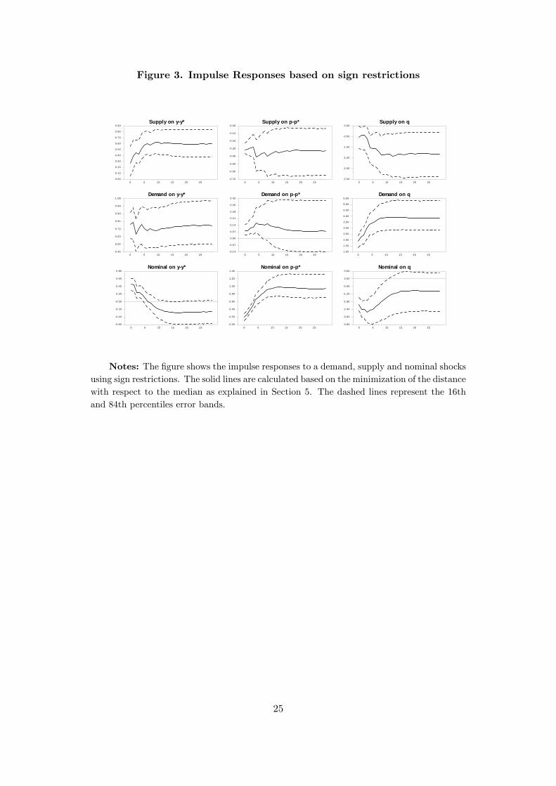
Figure 3. Impulse Responses based on sign restrictions

Supply on y­y*

0 5 10 15 20 250.00

0.10

0.20

0.30

0.40

0.50

0.60

0.70

0.80

0.90

Demand on y­y*

0 5 10 15 20 250.45

0.54

0.63

0.72

0.81

0.90

0.99

1.08

Nominal on y­y*

0 5 10 15 20 25­0.60

­0.40

­0.20

­0.00

0.20

0.40

0.60

0.80

Supply on p­p*

0 5 10 15 20 25­0.70

­0.60

­0.50

­0.40

­0.30

­0.20

­0.10

­0.00

Demand on p­p*

0 5 10 15 20 25­0.14

­0.07

0.00

0.07

0.14

0.21

0.28

0.35

0.42

Nominal on p­p*

0 5 10 15 20 250.00

0.20

0.40

0.60

0.80

1.00

1.20

1.40

Supply on q

0 5 10 15 20 25­2 .50

­2 .00

­1 .50

­1 .00

­0 .50

0.00

Demand on q

0 5 10 15 20 251.00

1.50

2.00

2.50

3.00

3.50

4.00

4.50

5.00

5.50

Nominal on q

0 5 10 15 20 25­3 .60

­3 .00

­2 .40

­1 .80

­1 .20

­0 .60

0.00

0.60

Notes: The �gure shows the impulse responses to a demand, supply and nominal shocksusing sign restrictions. The solid lines are calculated based on the minimization of the distancewith respect to the median as explained in Section 5. The dashed lines represent the 16thand 84th percentiles error bands.

25

Figure 4. Structural shocks

Clarida­Gali approachSu

pply

1976 1979 1982 1985 1988 1991 1994 1997 2000 2003 2006­3.6

­2.4

­1.2

0.0

1.2

2.4

Dem

and

1976 1979 1982 1985 1988 1991 1994 1997 2000 2003 2006­2.4

­1.6

­0.8

­0.0

0.8

1.6

2.4

Nom

inal

1976 1979 1982 1985 1988 1991 1994 1997 2000 2003 2006­3

­2

­1

0

1

2

3

Sign restrictions approach

Supp

ly

1976 1979 1982 1985 1988 1991 1994 1997 2000 2003 2006­2.7

­1.8

­0.9

­0.0

0.9

1.8

2.7

Dem

and

1976 1979 1982 1985 1988 1991 1994 1997 2000 2003 2006­3.2

­2.4

­1.6

­0.8

­0.0

0.8

1.6

2.4

3.2

Nom

inal

1976 1979 1982 1985 1988 1991 1994 1997 2000 2003 2006­2.7

­1.8

­0.9

­0.0

0.9

1.8

2.7

Figure 5. Historical decomposition

Supply Demand Nominal

Clarida­Gali approach

1976 1979 1982 1985 1988 1991 1994 1997 2000 2003 2006­20

­10

0

10

20

30

Supply Demand Nominal

Sign restrictions approach

1976 1979 1982 1985 1988 1991 1994 1997 2000 2003 2006­25

­20

­15

­10

­5

0

5

10

15

20

26

Figure 6. Impulse responses based on alternative sign restrictions

Supply on y­y*

0 5 10 15 20 250.00

0.20

0.40

0.60

0.80

1.00

1.20

1.40

Demand on y­y*

0 5 10 15 20 250.16

0.32

0.48

0.64

0.80

0.96

1.12

1.28

Nominal on y­y*

0 5 10 15 20 25­0.50

­0.25

0.00

0.25

0.50

0.75

1.00

Supply on p­p*

0 5 10 15 20 25­0.90

­0.80

­0.70

­0.60

­0.50

­0.40

­0.30

­0.20

­0.10

Demand on p­p*

0 5 10 15 20 25­0.08

0.00

0.08

0.16

0.24

0.32

0.40

0.48

0.56

0.64

Nominal on p­p*

0 5 10 15 20 250.00

0.20

0.40

0.60

0.80

1.00

1.20

1.40

Supply on q

0 5 10 15 20 25­2 .00

­1 .50

­1 .00

­0 .50

0.00

0.50

1.00

1.50

2.00

2.50

Demand on q

0 5 10 15 20 250.50

1.00

1.50

2.00

2.50

3.00

3.50

4.00

4.50

5.00

Nominal on q

0 5 10 15 20 25­4 .00

­3 .50

­3 .00

­2 .50

­2 .00

­1 .50

­1 .00

­0 .50

0.00

0.50

Notes: The �gure compares the impulse responses to a demand, supply and nominalshocks using the baseline sign restrictions of Figure 4.3 (hatched lines) with the ones obtainedusing alternative sign restrictions (solid and dashed lines). The alternative speci�cationrelaxes the restriction on the real exchange rate in the case of a supply shock.

27

Figure 7.A. Impulse responses subsample 1976:01-1989:04

Supply on y­y*

0 5 10 15 20 250.10

0.20

0.30

0.40

0.50

0.60

0.70

0.80

Demand on y­y*

0 5 10 15 20 250.20

0.40

0.60

0.80

1.00

1.20

Nominal on y­y*

0 5 10 15 20 25­1.00

­0.75

­0.50

­0.25

0.00

0.25

0.50

0.75

Supply on p­p*

0 5 10 15 20 25­0.70

­0.60

­0.50

­0.40

­0.30

­0.20

­0.10

­0.00

0.10

0.20

Demand on p­p*

0 5 10 15 20 25­0.60

­0.40

­0.20

­0.00

0.20

0.40

0.60

Nominal on p­p*

0 5 10 15 20 250.00

0.50

1.00

1.50

2.00

2.50

Supply on q

0 5 10 15 20 25­2 .80

­2 .40

­2 .00

­1 .60

­1 .20

­0 .80

­0 .40

­0 .00

0.40

Demand on q

0 5 10 15 20 250.00

1.00

2.00

3.00

4.00

5.00

6.00

Nominal on q

0 5 10 15 20 25­5 .00

­4 .00

­3 .00

­2 .00

­1 .00

0.00

1.00

Figure 7.B. Impulse responses subsample 1990:01-2006:04

Supply on y­y*

0 5 10 15 20 250.00

0.25

0.50

0.75

1.00

1.25

1.50

Demand on y­y*

0 5 10 15 20 250.20

0.40

0.60

0.80

1.00

1.20

1.40

Nominal on y­y*

0 5 10 15 20 25­0.10

0.00

0.10

0.20

0.30

0.40

0.50

Supply on p­p*

0 5 10 15 20 25­0 .45

­0 .40

­0 .35

­0 .30

­0 .25

­0 .20

­0 .15

­0 .10

­0 .05

Demand on p­p*

0 5 10 15 20 250.00

0.05

0.10

0.15

0.20

0.25

0.30

0.35

0.40

0.45

Nominal on p­p*

0 5 10 15 20 250.05

0.10

0.15

0.20

0.25

0.30

0.35

0.40

Supply on q

0 5 10 15 20 25­3 .50

­3 .00

­2 .50

­2 .00

­1 .50

­1 .00

­0 .50

0.00

0.50

Demand on q

0 5 10 15 20 251.60

2.40

3.20

4.00

4.80

5.60

6.40

7.20

Nominal on q

0 5 10 15 20 25­2 .00

­1 .50

­1 .00

­0 .50

0.00

0.50

1.00

1.50

Notes: The �gure shows the impulse responses to a demand, supply and nominalshocks using sign restrictions for two subperiods. The solid lines are calculated based onthe minimization of the distance with respect to the median as explained in Section 5. Thedashed lines represent the 16th and 84th

28

Figure 8. Impulse responses alternative REER

Supply on q

0 5 10 15 20 25­1.50

­1.25

­1.00

­0.75

­0.50

­0.25Demand on q

0 5 10 15 20 251.00

1.50

2.00

2.50

3.00

3.50

4.00Nominal on q

0 5 10 15 20 25­2.75

­2.50

­2.25

­2.00

­1.75

­1.50

­1.25

­1.00

­0.75

Notes: The �gure compares the impulse responses of the real exchange rate to a demand,supply and nominal shocks using the baseline model presented in Figure 3 (solid lines) withthe ones obtained when the model is estimated using the real e¤ective exchange rate sourcedfrom the Federal Reserve Board of Governors (dashed lines).

Figure 9. Impulse Responses extended model

Supply on y­y*

0 5 1 0 1 5 2 0 2 50 .0 9

0 .1 8

0 .2 7

0 .3 6

0 .4 5

0 .5 4

0 .6 3

0 .7 2

0 .8 1

Demand on y­y*

0 5 1 0 1 5 2 0 2 50 .4 0

0 .5 0

0 .6 0

0 .7 0

0 .8 0

0 .9 0

1 .0 0

1 .1 0

Monetary on y­y*

0 5 1 0 1 5 2 0 2 5­0 .4 2

­0 .2 8

­0 .1 4

0 .0 0

0 .1 4

0 .2 8

0 .4 2

0 .5 6

Supply on p­p*

0 5 1 0 1 5 2 0 2 5­0 .8 0

­0 .7 0

­0 .6 0

­0 .5 0

­0 .4 0

­0 .3 0

­0 .2 0

­0 .1 0

Demand on p­p*

0 5 1 0 1 5 2 0 2 5­0 .4 0

­0 .3 0

­0 .2 0

­0 .1 0

­0 .0 0

0 .1 0

0 .2 0

0 .3 0

0 .4 0

Monetary on p­p*

0 5 1 0 1 5 2 0 2 50 .0 0

0 .1 6

0 .3 2

0 .4 8

0 .6 4

0 .8 0

0 .9 6

1 .1 2

Supply on i­i*

0 5 1 0 1 5 2 0 2 5­0 .3 6

­0 .3 0

­0 .2 4

­0 .1 8

­0 .1 2

­0 .0 6

0 .0 0

0 .0 6

Demand on i­i*

0 5 1 0 1 5 2 0 2 5­0 .1 0

0 .0 0

0 .1 0

0 .2 0

0 .3 0

0 .4 0

0 .5 0

0 .6 0

0 .7 0

Monetary on i­i*

0 5 1 0 1 5 2 0 2 5­0 .5 4

­0 .4 5

­0 .3 6

­0 .2 7

­0 .1 8

­0 .0 9

­0 .0 0

0 .0 9

0 .1 8

0 .2 7

Supply on q

0 5 1 0 1 5 2 0 2 5­3 .0 0

­2 .5 0

­2 .0 0

­1 .5 0

­1 .0 0

­0 .5 0

0 .0 0

Demand on q

0 5 1 0 1 5 2 0 2 51 .0 0

2 .0 0

3 .0 0

4 .0 0

5 .0 0

6 .0 0

Monetary on q

0 5 1 0 1 5 2 0 2 5­3 .0 0

­2 .5 0

­2 .0 0

­1 .5 0

­1 .0 0

­0 .5 0

0 .0 0

0 .5 0

1 .0 0

1 .5 0

Notes: The �gure shows the impulse responses to a demand, supply and nominal shocksusing sign restrictions for the 4 variable VAR. The solid lines are calculated based on theminimization of the distance with respect to the median as explained in section 3. The dashedlines represent the 16th and 84th percentiles error bands.

29

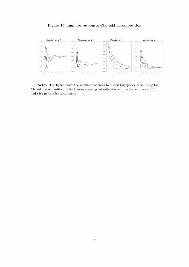
Figure 10. Impulse responses Choleski decomposition

Monetary on y­y*

0 5 1 0 1 5 2 0 25­0.15

­0.10

­0.05

0 .0 0

0 .0 5

0 .1 0

0 .1 5Monetary on p­p*

0 5 1 0 15 2 0 2 5­0 .05

­0 .03

0.0 0

0.0 3

0.0 5

0.0 8

0.1 0

0.1 2

0.1 5Monetary on i­i*

0 5 1 0 1 5 20 2 5­0 .1 0

0.00

0.10

0.20

0.30

0.40

0.50

0.60

0.70

0.80Monetary on q

0 5 10 1 5 2 0 2 5­0 .1 6

0.00

0.16

0.32

0.48

0.64

0.80

0.96

1.12

Notes: The �gure shows the impulse responses to a monetary policy shock using theCholeski decomposition. Solid lines represent point estimates and the dashed lines are 16thand 84th percentiles error bands.

30

A Appendix

Table A1. Tests for unit rootsy � y� p� p� i� i� q y � y� p� p� i� i� q

Levels Fist Di¤erences

ADFAIC -1.54(0.810)

-1.49(0.827)

-3.22�(0.085)

-2.31(0.426)

-5.85(0.000)���

-5.78(0.000)���

-4.83(0.000)���

-8.71(0.000)���

ADFBIC -1.49(0.828)

-0.33(0.917)

-2.48(0.335)

-1.81(0.692)

-10.22(0.000)���

-4.06(0.000)���

-8.98(0.000)���

-8.71(0.000)���

KPSS 0.29��� 1.17��� 0.09 0.71�� 0.07 0.04 0.05 0.07

Notes: The table shows the Augmented Dickey-Fuller (ADF) and the Kwiatkowski et al.(1992) (KPSS) test statistics. The former tests the null of unit root against a trend-stationaryalternative. The latter tests the null of trend-stationarity. The critical values of the ADF testare -3.15, -3.45 and -4.03 for the 10%, 5% and 1% signi�cance levels respectively. The criticalvalues for the KPSS test are 0.12, 0.15 and 0.22 for the 10%, 5% and 1% signi�cance levelsrespectively. AIC denotes that the lag length was selected according to the Akaike Criterionand BIC denotes that it was selected based on the Schwartz criterion. In parenthesis arep-values. The sample period is 1976-2006. *, **, *** indicates rejection of the null at 10%,5% and 1% respectively.

Table A2. Test of cointegrating rankrank=r Trace 95% crit. value p-value Trace 95% crit. value p-value

Baseline Model Extended Model

r=0 33.531 42.770 0.315 55.295 63.659 0.214r=1 18.194 25.731 0.338 31.806 42.770 0.405r=2 5.886 12.448 0.485 14.984 25.731 0.583r=3 - - - 4.542 12.448 0.667

Notes: The table shows the trace statistic corresponding to the Johansen (1991) testfor the number of cointegrating vectors. The statistics apply a small-sample correction. Thevariables of the baseline model are y � y�, p� p� and q and the variables of the extendedmodel are y � y�, p� p�, i� i�and q. The sample period is 1976-2006. The VAR model isestimated with 4 lags.

31

References

[1] Artis, M. and M. Ehrmann (2006). �The Exchange Rate �A Shock-Absorber orSource of Shocks? A Study of Four Open Economies.�Journal of InternationalMoney and Finance 25, 874-893.

[2] Beaudry P. and M.B. Devereux (1995). Money and the real exchange rate withsticky prices and increasing returns. Carnegie-Rochester Conference Series onPublic Policy 43, 55�102.

[3] Blanchard, O. and D. Quah (1989). �The Dynamic E¤ects of Aggregate Demandand Supply Disturbances.�American Economic Review 79, 655-673.

[4] Canova, F. and G. De Nicoló (2002). �Monetary Disturbances Matter for Busi-ness Fluctuations in the G-7.�Journal of Monetary Economics 49, 1131-1159.

[5] Canova, F. and J. Pina (1999). �Monetary Policy Misspeci�cation in VAR Mod-els.�CEPR Discussion Paper No 2333.

[6] Chari, V.; Kehoe, P. and E. McGrattan (2002). �Can Sticky Price Models Gener-ate Volatile and Persistent Real Exchange Rates?�Review of Economies Studies69, 533-363

[7] Chari, V.; Kehoe, P. and E. McGrattan (2007). �Are structural VARs with long-run restrictions useful in developing business cycle theory?� Sta¤ Report 364,Federal Reserve Bank of Minneapolis .

[8] Christiano, L.J.; Eichenbaum, M. and C.L. Evans (1999). �Monetary PolicyShocks: What Have We Learned and To What End?�In Taylor, J.B. and Wood-ford, M. (eds), Handbook of Macroeconomics, Vol. 1, Ch. 2, Elsevier, Amsterdamand New York, 65-148.

[9] Clarida, R. and J. Gali (1994). �Sources of real exchange-rate �uctuations: Howimportant are nominal shocks?�Carnegie-Rochester Conference Series on PublicPolicy 41, 1-56.

[10] Dornbusch, R. (1976). �Expectations and Exchange Rate Dynamics.� Journalof Political Economy 84, 1161-76.

[11] Eichenbaum, M. and C.L.Evans. (1995). �Some Empirical Evidence on the Ef-fects of Shocks to Monetary Policy on Exchange Rates.�Quarterly Journal ofEconomics 110, 975-1009.

[12] Engel, C. (1996). �The Forward Discount Anomaly and the Risk Premium: ASurvey of Recent Evidence.�Journal of Empirical Finance 3, 123-192.

[13] Fama, E. (1984). �Spot and Forward Exchange Rates�. Journal of MonetaryEconomics 14, 319-338.

[14] Farrant K. and G. Peersman (2006), �Is the Exchange Rate a Shock Absorberor Source of Shocks? New Empirical Evidence.�Journal of Money, Credit andBanking 38, 939-962.

[15] Faust, J. (1998). �The Robustness of Identi�ed VAR Conclusions AboutMoney.�Carnegie-Rochester Conference Series in Public Policy 49, 207-244.

[16] Faust, J. and E.M. Leeper (1997). �When Do Long-Run Identifying RestrictionsGive Reliable Results?� Journal of Business and Economic Statistics 15, 345-353.

32

[17] Faust, J. and J.H. Rogers (2003). �Monetary policy�s role in exchange rate be-havior.�Journal of Monetary Economics 50, 1403-1424.

[18] Fratzscher, M.; Juvenal L. and L. Sarno (2007). �Asset prices, Exchange Ratesand the Current Account.�Working Paper Series 790, European Central Bank.

[19] Fry R. and A. Pagan (2007). �Some Issues in Using Sign Restrictions for Iden-tifying Structural VARs.�NCER Working Paper Series 14, National Centre forEconometric Research.

[20] Johansen, S. (1991). �Estimation and Hypothesis Testing of Cointegration Vec-tors in Gaussian Vector Autoregressive Models.�Econometrica 59, 1551-80.

[21] Kim, S. (1999). �Do monetary policy shocks matter in the G-7 countries? Us-ing common identifying assumptions about monetary policy across countries.�Journal of International Economics 48, 387�412.

[22] Kim, S. and N. Roubini (2000). �Exchange Rate Anomalies in the IndustrialCountries: A Solution with a Structural VAR Approach.�Journal of MonetaryEconomics 45, 561-586.

[23] Mountford, A. and H. Uhlig (2005). �What are the E¤ects of Fiscal PolicyShocks?�Humboldt University, mimeo.

[24] Obstfeld, M. (1985). �Floating Exchange Rates: Experience and Prospects.�Brookings Papers on Economic Activity 2, 369-450.

[25] Obstfeld, M. (1995). �International Currency Experience: New Lessons andLessons Relearned.�Brookings Papers on Economic Activity 1, 119-196.

[26] Obstfeld and Rogo¤ (1995). �Exchange Rate Dynamics Redux.�Journal of Po-litical Economy, University of Chicago Press, vol. 103(3), pages 624-60, June.

[27] Paustian, M. (2007). �Assessing Sign Restrictions.�The B.E. Journal of Macro-economics 7, 1-31.

[28] Peersman, G. (2005). �What Caused the Early Millennium Slowdown? EvidenceBased on Vector Autoregressions.�, Journal of Applied Econometrics 20, 185-207.

[29] Rogers, J. H. (1999). �Monetary shocks and real exchange rates.� Journal ofInternational Economics 49, 269-288.

[30] Rogo¤, K. (1996). �The Purchasing Power Parity Puzzle.�Journal of EconomicLiterature 34, 647-668.

[31] Sarno, L. and D.L. Thornton (2004). �The E¢ cient Market Hypothesis andIdenti�cation in Structural VARs.� Federal Reserve Bank of St. Louis Review86, 49-60.

[32] Scholl, A and H. Uhlig (2006). �New Evidence on the Puzzles: Monetary Pol-icy and Exchange Rates.�Computing in Economics and Finance 5, Society forComputational Economics.

[33] Sims, C.A. (1992). �Interpreting the macroeconomic time series facts: the e¤ectsof monetary policy.�European Economic Review 36, 975�1011.

[34] Sims, C.A. and T. Zha (2006). �Does Monetary Policy Generate Recessions?�Macroeconomic Dynamics 10, 231-272.

33

[35] Truman, E.M. (2006). �What Can Exchange Rates Tell Us?�In C. Fred Bergstenand the World Economy, Ed. M. Mussa, The Peterson Institute for InternationalEconomics.

[36] Uhlig, H. (2005). �What are the E¤ects of Monetary Policy on Output? Resultsfrom an Agnostic Identi�cation Procedure.�Journal of Monetary Economics 52,381-419.

34