Non-Classical Processes in Quantum Mechanics

Ulm University

Institute for Theoretical Physics

Non-Classical Processes in Quantum Mechanics

A resource theory approach to characterize coherence

Dissertation, submitted by

Dario Egloff

(born in Lenzburg), for the degree of Dr. Rer. Nat. of the Faculty of Natural Sciences at Ulm University, in

2018

Dissertation,submitted at Ulm University,Faculty for Natural Sciences.Dean of the Faculty: Prof. Dr. Peter Dürre

1st Reviewer: Prof. Dr. Martin B. Plenio2nd Reviewer: Prof. Dr. Susana F. HuelgaAdditional Examiners: Prof. Dr. Matthias Freyberger

Prof. Dr. Joachim AnkerholdChair for the defense: Prof. Dr. Ute Kaiser

Date of Defense: 19.02.2019

PREFACE

Four years ago, I was looking for a place to do my PhD thesis. At that time we were finishinga work on resource theories of thermodynamics, and I was unsure whether to continue working inthe same, operational, but mathematical direction or to change to either a more applied, or to a morefundamental part of physics. Intrigued by the clarity of the operational approach to coherence by thegroup of Martin [8], I was very happy to have the opportunity to visit Ulm. It became apparent inthat visit that the people in the group have a high focus and interest in physics paired with a certainrelaxedness. There was time and interest to talk about stupid questions from my side and also aboutthings not concerning physics. Indeed, this did not change in the last years, I can still ask stupidquestions and get good answers from people in the group.

Coming to Ulm meant to continue with a very operational and mathematical approach and mostof the thesis reflects that; very roughly and abstractly speaking, the thesis is about characterisingproperties by looking at the actions that lead to them. It was only in the last year that this changedslightly. On one side, we are currently involved in two experiments, one concerning chapter IV of thisthesis (on a more foundational issue) and another one having provided, by a very practical question,the initial motivation for the article leading to chapter VI. Unfortunately, both are not yet finishedand I cannot present any results on these experiments yet. On the other side, the main question ofthis thesis, namely how to characterize non-classical processes, while operational, of course has somelinks to foundational questions.

Almost all of the results of the works building the basis of this thesis were done in close collab-oration with Thomas, Mauricio and Andrea. Some of them were literally done together, in manydays spent in front of a whiteboard. All of the results also have important contributions of Martin,and many also of María, Nathan, Lijiang and Susana (as can be seen from the author list of the mainreferences). Chapter V is in great parts literally taken from the preprints of Refs. [3, 5], chapter VI ismostly a reordering of a preprint of [6] and chapter IV is based on new notes of me, Andrea and Su-sana, following [7]. That last paper also contains some results not presented here. As I was fortunateenough to work very closely with great physicists here in Ulm, in most parts of the thesis I cannotwrite what “I found”, but will say what “we found” instead.

The papers [2], based on the Master Thesis of María, and [4], based on the Master Thesis ofThomas, both of which I had the pleasure of co-supervising, are not covered in this thesis. Nor is thearticle [1], which, although having been published after my arrival in Ulm, stems from my MasterThesis.

I wish to thank my family, Adriana and her family, my friends and colleagues and all membersof the group. It was due to them that the last years have been very interesting, while extraordinarilypleasant. Special thanks go to Thomas, Andrea and Adriana for reading and commenting a draft ofthis thesis.

CONTENTS

Preface 3

I Background 6

I. Introduction 6

II. Resource Theories of Non-Stochasticity 10A. Classical processes in quantum mechanics 10B. Resource theories 13

III. Outline and Summary of the Main Results 18

II Results 22

IV. Non-Classical Dynamics 22A. N-Markovianity 25B. N-Classicality 27

1. NCGD dynamics 282. A philosophical side-note 32

V. Coherent States, Entanglement and Quantum Discord 34A. Local operations and physical wires 36

1. Setting 36B. Basis dependent discord and coherence 40

1. Proofs 472. General form of LOP for three-level systems 543. Counterexample: LOP, IQO 55

C. Measures and monotones 561. Monotones for coherence and basis-dependent discord 562. Thermal discord as an upper bound for the recoverable coherence 583. Proofs 604. Lower bounds 62

D. Quantum discord and LOP 63E. Classicality of states 64

1. All not incoherent-quantum states are resource states 642. Stochastic model for LOP 66

F. Resources in the DQC1 protocol 67G. Coherence cost of entanglement 70H. Relation to different classes of operations 77

VI. Coherent Maps 80A. Measuring the coherence detecting ability of maps 81

1. Proofs 84B. Connection to the framework of non-classicality 88C. Detecting coherence 90

1. Proofs and a helpful lemma 93D. Semidefinite program for the diamond-measure 98E. Operational interpretation of the nSID-measure 102F. Evaluating the nSID-measure 104G. Examples 107H. A measure for detection-creation incoherent operations 108

VII. Conclusion and Open Questions 112

References 114

Appendix 122

A. Dynamical maps in finite dimensions 122

B. Copyrights 130

Part I

Motivation and Background

I. INTRODUCTION

The history of quantum mechanics is first and foremost a history of ground-breaking discoveriesand technological advance. As is always the case with discoveries, quantum mechanics seemed likemagic at its start. What is unusual about this theory is that, while we got better in using it and gotaccustomed to some of its peculiarities, even after almost a century, many aspect of it still seemmagical or – worse – paradoxical (see e.g. the recent article [9] and references therein). This canonly mean that the physics of small systems is still not fully understood. As an interested layman infoundations of quantum physics I did get the impression that in the last years there has been somegreat advance in this topic, and I am hopeful that the next few years will become very interesting.

The problem of understanding quantum mechanics did not change since its beginning – in theend it is always the waive-particle duality that provides the magic. It is the problem of being ableto perfectly describe the behaviour of an ensemble statistically, as an interacting continuum, whileknowing that the statistics comes from single events, quanta. That by itself is not a problem, if it wasnot the case that in many situations, the quanta need to follow a pattern that seems orchestrated, asif they interacted with a non-existent copy of themselves. This can be made more stringent if oneconsiders copies of parties that are far away from each other and measured simultaneously. In thatcase, according to the best theory of time we have at the moment, relativity theory (special relativityis enough for this example), it can happen that it is impossible to say which measurement is done first,while the predictions make it seem as if each depended on the other one. That is what Einstein calledspooky action at a distance in his famous paper with Podolsky ad Rosen (EPR) [10]. As Einsteinfirmly believed in both a clear causal order as also in that one can actually do experiments locallywithout others interfering from afar, that paper concluded that the variables that describe quantummechanics do not describe reality and hence one needs to complete the picture. It was Bell thatpointed out that if there was a theory that describes reality with local deterministic variables, thattheory needs to be at odds with the predictions of Quantum Mechanics [11] (also see his review [12]).By now this has been extensively tested, with the first test that for most physicists was consideredconclusive done by Aspect, Grangier and Roger [13] (based on a further developed formulation ofBell’s theorem due to Clauser, Horne, Shimony and Holt, CHSH [14]). Since then the tests have beenimproved (see e.g. [15]) and reproduced in various systems [16, 17] and the last reasonable loopholeshave been closed [18] (by using efficient detectors, fast random basis selection and a sufficiently largedistance without losses). The result of all these tests is clearly in favour of quantum mechanics,such that one really needs compelling arguments if one wants to argue on the line of the EPR paper.Unfortunately, it is easy to misinterpret or oversimplify these clear experimental results. For instance,it is not true that the experiments on Bell’s theorem rule out hidden variable theories (Bohm’s theoryis a hidden variable theory making the same predictions as quantum mechanics [19]). It is also wrongto say that these experiments show that quantum mechanics is non-local, for two reasons. The firstreason, which might struck as slightly picky, is that quantum mechanics is a theory, and on that level

p. 6

the statement is simply not meaningful (if one wants to have a meaningful notion of non-locality, itneeds to depend on the interpretation of what reality is, which cannot be part of the theory). However,the description of the states in quantum mechanics is non-local, but this does not follow from theexperiments, but directly from the theory, for instance by the argument of EPR. The second reason is,that even though the outcomes of a measurement done far away can influence the predicted outcomesof a measurement done in your lab (if you get to know them), the mere fact that a measurement isperformed has no effect on the statistics. So maybe we are indeed looking at the wrong variables,but in a much more intricate way than thought. A research line in that direction is relational quantummechanics, which weakens the idea of an absolute objective reality in favour of an objective realitythat only determines relations between objects [20]. Unfortunately (to my knowledge) until now ithas more the flavour of a project than of a full-fledged theory; a very intriguing project, I might add. Amore evolved interpretation in a similar direction, though completely different in character, is QBism,which weakens the notion of objective reality, making it fundamentally out of reach and replacing itwith subjective (and inter-subjective) descriptions of reality [21, 22]. It does not deny that there mightbe a reality out there, but there is no way to tell what it is. Even so it is not solipsistic. The argumentis, that a reasonable person will not gamble on something that his or her experience tells to be unlikely(including reasoning on the basis of abstract theories, learned by trusting the experience of others).Personally, I would describe it as the most rational point of view of quantum mechanics (and scienceas a whole). I think it is important to keep this perspective in mind for assessing the relevance of theknowledge one already has. However for me, though maybe that is just my misinterpretation, it lacksthe reflex of asking for the cause when seeing a shadow, even if the answer is out of reach.

In any case, QBism reflects the shift that happened in the last decades. The shift from trying totest the strange properties of quantum mechanics (for small systems with not too high energy), to takethem for granted and see how one can make use of them for technological applications [23]. This doesnot imply that they are understood, but just that any serious physicist would bet on the prediction onegets from assuming them to be real (if one is able to make a prediction, that is). In colloquial terms,one could say that they are now generally accepted as real. This started with the characterizationof entanglement as the property that cannot be prepared on two separated systems by two separatedparties (Alice and Bob) even if they communicate with each other and its applications [24, 25]. Intu-itively one would expect that the only thing one cannot prepare locally is something that is not localand hence an extensive object. But if the systems are separated and do not share an extensive object,what is it they share? I don’t know, but it is called entanglement. In this way the just described settingincorporates the idea of EPR and Bell that locality is a pre-requirement for classical physics. It has theself-explaining name local operations and classical communication (LOCC), and we will encounter itin many parts of this thesis.

It was soon understood that entangled systems allow to provably communicate securely betweendifferent parties [26], produce provably random keys and improve sensing [27, 28]. Furthermore, inprinciple, they allow to make computations that are completely out of reach for classical computers,such as simulating complex quantum systems [29] or factorizing large numbers [30]. It also seemsreasonable to expect that (soon) quantum computers (at least when combined with classical ones) willalso outperform classical computers for many other tasks for which the speed-up is hard to prove, withmachine learning being the most prominent example. This is the case, because quantum computers

PhD Thesis p. 7

I. Introduction

increase the amount of interdependent paths that a computation can take exponentially with the sizeof the system. Also with quantum computers one still only gets one outcome per round (actually,being probabilistic, one can argue that one gets even less than one). Due to the nature of quantummechanics, however, the outcome can be the result of many possible paths at once, without the needto compute them separably.

While entanglement theory was very successful, evidence grew that there are tasks which do notseem possible classically, but which work even without needing entanglement. For this reason, an-other, more common property of quantum states was claimed to be non-classical as well; this propertyis called quantum discord [31–35]. In a way this is not surprising, as entanglement is just the mostclear-cut non-classical feature of quantum mechanics, but it is not the only one. The basic equa-tion of quantum mechanics, namely Schrödinger’s, is a wave equation and its object, the quantumstates, are probability amplitudes. From this it follows that one can have superpositions of statesleading to correlated behaviour of the probabilities, which in turn can be unintuitive (the orchestratedquanta described above). Entanglement is such a superposition that can be unintuitive due to apparentnon-local behaviour, as explained above. Another way in which superpositions becomes particularlyunintuitive, is when one uses quantum mechanics to describe states that only have a meaning on amacroscopic level, such as if a cat is dead or alive. Blindly applying the rules of quantum mechanicscan lead to making the cat being in a state that is neither dead or alive, but by a well-described super-position of the two instead – meaning that you know how the cat is, but it is neither dead nor alive,which obviously does not make much sense [36]. In a similar way, one can also build no-go theoremsfor classical physics that replace the assumption on locality of the actions from Bell’s theorem witheither that reality does not depend on how you test it [37–40] or that (macroscopically) it should bepossible to observe a dynamics without disturbing it [41–44]. For the cat this means that it is deadwith some probability and otherwise alive; opening the box just shows what is – at least if you don’taccidentally kill it while lifting the lid1.

Recently, the property of a system being in a superposition (of orthogonal basis states) has beenformalised in a resource theoretic approach, the resource theory of quantum coherence [8, 45]. Thismade it possible to analyse coherence on a more formal and precise level, leading to many results ina very short time (see [46] for a review). It soon became clear that the property is tightly connectedto entanglement [47, 48]. However, the initial formulation of the theory, while clear conceptually, isnot so easy to interpret physically, which lead very early on to a bunch of alternative theories (seee.g. [49]).

In the works leading to this thesis the aim was to give a clear operational interpretation of differentaspects of non-classicality. Doing so, enables to see the different properties as different aspects ofthe same underlying question, namely whether there is a classical explanation of the measurements athand. If one incorporates the additional assumptions in the setting (such as locality by the separationof the two parties in entanglement theory), the question of whether some system is classical, boilsdown to ask whether one can simulate everything one can possibly observe by classical variablesgoverned by a stochastic process. This new perspective allows to characterise dynamic properties of

1 This is a serious comment. In fact this issue makes the Leggett-Garg-type arguments substantially weaker than the Bell-type argu-ments. In the former, one compares the same system measured at different points in time, but one can never fully exclude that just byperforming a measurement one changes what happens afterwards. In the Bell-type case, one compares the outcomes of two spatiallyseparated measurements done at the same time; if one assumes that effects spread with a finite speed (not faster than the speed oflight), the measurements cannot affect each other.

p. 8 Non-classical Processes

non-classicality, and also to connect them to more static types of non-classicality such as entangle-ment. Indeed we unify entanglement, discord and coherence from one single perspective. We dothis by restricting our setting such that the operations have a clear classical interpretation and henceincorporating natural restrictions of classical systems, if the initial state of the system is not entangleddoes not have discord or does not have coherence. If the initial state of the system is different, we seethe magic of quantum mechanics happening again. For instance we show for one specific quantumalgorithm, which is thought to be better than any classical algorithm for its task, that the precisionof the algorithm scales with the coherence present at its start. In other words, it is these resources(coherence, discord and entanglement) that make the magic possible and with our perspective we caninterpret the role of the different resources and analyse how they are linked to each other. This doesnot give an explanation of the magic of quantum mechanics, but it does make the mechanisms moretransparent allowing for new explanations and there are some examples already in this thesis. Finallywe also look at the dual of when states are non-classical, asking, and answering, in a specific set-ting, what makes measurements non-classical. A summary of the results can be found in chapter III,starting on page 18.

PhD Thesis p. 9

II. RESOURCE THEORIES OF NON-STOCHASTICITY

A. Classical processes in quantum mechanics

The aim of this thesis is to characterize when and how a quantum model cannot be simulatedclassically. There are two notions to define here before proceeding further, quantum model and tosimulate classically. We start with the latter.

In classical physics, given a physical system, there is an (ideal) measurement that without changingthe state of affairs maps it at any time to a correspondent, self-consistent mathematical description,given by a real number or real vector of the system at that time (which fully describes the system, butone can drop this requirement). More precisely one asks that there is a family of random variablesdefined on the set of events, which is parametrized by the time. This is the definition of a stochasticprocess. Operationally it trivially follows that not performing the ideal measurement is the same asforgetting the outcomes after performing it. This property is one of the Kolmogorov consistencyconditions, where the others are just the usual conditions defining probability distributions (positivityand summing to one). Henceforth we will call only this one the Kolmogorov consistency conditionand silently assume the other ones if we talk of probabilities. It is not trivial that also the conversestatement is true (see any book on stochastic processes, e.g. [50]). If and only if the conditions holdsfor all measurement times and any number of measurements and any outcomes, by Kolmogorov’stheorem, there is a classical stochastic process that predicts the same statistics.

The problem is that testing the condition is impractical, as one has an infinite set of conditions. Inan experiment one might just be interested in measuring at certain times T and making at most a finitenumber of measurements N. In this case, if for times in T and up to N measurements the conditionholds, Kolmogorov’s theorem still guarantees the existence of a classical stochastic process that forthe same parameters gives the same multi-time statistics (up to N), though the process might dependon which N measurements one does, in the non-Markovian case. This means that the process mightnot be classical in theory, but if we do not make more measurements, or measure at different times,we will not be able to notice a difference. That is, we can simulate the process classically. In anycase, without needing any additional assumption, if one of the conditions does not hold the process isnot classical. We therefore define N-Classical processes in the following way.

Definition II.1 (N-classical statistics). We call a multi-time statistics that is described by the multi-time probabilities Qn {(in, tn) , . . . (i1, t1)}, N-classical in T , iff the Kolmogorov consistency conditionholds up to n = N at times in T . That is∑

ik

Qn {(in, tn) , . . . (i1, t1)} (1)

= Qn−1{(in, tn) , . . .

(/ik, /tk

). . . (i1, t1)

},

for any k, any time-ordered ~t with ti ∈ T and any n ≤ N, with N at least 2.If there is no such N, we call the process non-Classical in T .

With this definition in mind, we can now operationally define what we mean by the sentence thata quantum process can be simulated classically. It just means that given a set of times T and a family

p. 10

A. Classical Processes

of observables Mt, we have a quantum system undergoing a given evolution, which we measure atthose times (up to N times), giving raise to a multi-time statistics that can be simulated by a stochasticprocess, i.e. the process is (N-)classical in T .

We also want to describe more generic situations, in which one may also perform different tasksor measurements at intermediate times or change the initial state of the system. In these cases theevolution is not fixed any more and hence we also introduce a more generic notion, which we call aquantum model for an experimental setting. For it to be classical, we simply require that any possibleprocess will be classical.

We will now proceed with abstract definitions of what we just said. This is needed if one wantsto discuss different notions of non-classicality from the same (operational) point of view. However itis usually not necessary to discuss any single one of them, as quite generally one makes (and we willmake) strong simplifying assumptions, which differ in each case, making them seem unrelated. Inother words, what follows, in the rest of this chapter, is to be understood as a digression on a genericdefinition of theoretical models, that can then be applied to different quantum mechanical models tosee if they can be simulated by classical models. This is not crucial for understanding the thesis, butmakes some notions more precise and I believe it to be useful for further research. Here we considera general theory. A theory needs to define possible descriptions of a system, that is a family of statespaces S = {Sx}x (it is possible to have only one, and in the following we will often use S insteadof Sx, if we mean any state space). It also needs to describe measurements M on the state spaces,where each consists of a mapping from a state space to probability space m ∈ M : Sx → [0, 1]n (sincein practice one can only do a finite number of measurements, a theory needs to have meaningfulmeasurements with a finite number of outcomes n ∈ N). One should also have maps (or operations)O in the theory, such that a state is mapped to another state Λ ∈ O : Sx → Sy. As one needs to geta description somehow, one also needs map that yield a description even if one does not know thestate at the beginning (it is something), that is, one needs that the maps include preparations and thatthere is a trivial state space consisting of a single element, which we will call {1} (alternatively, onecould imagine to have a special state in some state spaces, where each describes this minimal state ofknowledge instead, but one can easily map this case to the other by literally a one-to-one map). Asan alternative, one could also combine measurements, preparations and maps into one single object,called instrument in the literature (see [51] and citing articles), which consists of a couple of vectors(~m, ~I) ∈ I (trivially identified with a vector of couples (mi, Ii)i ≡ (~m, ~I)), such that with probabilitymi : Sx → [0, 1] the map is Ii : Sx → Sy). If one is interested in two-time statistics, this is all oneneeds. However it will also be useful to look at the actions one can do on a given dynamics, thatis, given a family of operations {Λt}t ⊂ O, how can it be altered (in the most general case, includingmeasurements in between)? We therefore define actions as the mapping from a dynamics to a familyof instruments Θ ∈ A : {Λt}t 7→ {m~is

[{Λt}t], I~is[{Λt}t]}~i,s, where in principle the instrument at time s

can depend on all precedent measurement outcomes~is := {is, . . . , i1}, i.e. have a memory. We leavethese definitions very general, as even though all we will discuss in this thesis concerns quantummechanics, one can have different definitions of the theory even within this framework; for instanceone can consider only unitary dynamics on pure states or any open system dynamics on mixed statesor (what we will generally do) something in between these extremes.

We want to construct resource theories of non-classicality. For this aim, we will restrict what we

PhD Thesis p. 11

II. Non-stochasticity

can do and check that these restrictions insure classicality of the possible processes. If this is the case,and there are some additional states, operations, actions, or measurements in the theory that allow todo non-classical processes, we can characterize the non-classicality of these. Given a theory T , Wecall a tuple (FM,FS,FO,FA) (or, alternatively (FI,FA)) a T model, if it is a restriction of the theory,that is (FM ⊂ M,FS ⊂ S,FO ⊂ O,FA ⊂ A). In principle one can think that at different times onecan do different actions or operations or measurements. To include this, we simply have to add anindex t to the state spaces at different times. Similarly the free operations then get a label for time,defining possible free dynamics. In principle also the free measurements can be time-dependent. Onetrivially gets some minimal requirements for the free sets, namely that the free dynamics applied tothe free states have to yield free states at any time and similarly that the free actions applied to thefree dynamics lead to free dynamics and measurements. As operationally one does some actions ona given dynamics, one may also ask that all the free states, free measurements and free dynamics canbe reached by some actions applied to at least one free dynamics and initial state.

Then one can consider multi-time statistics in the most general way by doing actions Θ on a givendynamics {Λt}t and a given starting state ρ

Qn {(in, tn) , . . . (i1, t1)} [Θ] = (min,...,i1[{Λt}t])[ρ]. (2)

While one can make sense of processes, where the dynamics has memory effects, using complex ac-tions with a memory (which in quantum mechanics can always be approximated by process tensorsor quantum combs [52–56]), we leave the rather involved analysis open for future work and restrictourselves to more simplistic models. Even being simpler, these will however turn out to be general-izations of known concepts (entanglement theory, coherence theory, quantum discord or Leggett-Gargtype inequalities) or indeed already be completely new, enabling us to make a step further and lookat dynamic properties as resources. That is, we will restrict our actions to either make measure andprepare operations at different time-points, or to map operations to other operations. To be able tomake sense of that, however, we will need to restrict both the classical as well as the quantum modelsto Markovian ones (vaguely referring to dynamics without memory effects. The term is unambiguousfor classical stochastic dynamics, but ambiguous in quantum mechanics. More on this later). Thismight seem unsatisfactory, as usually processes are not Markovian, but remember that one can alwaysconstruct a Markovian model from a non-Markovian one by increasing the state space. This is trueboth in classical physics, where one needs to add a memory, as well as in quantum physics, whereevery evolution can be thought to be a reduced dynamics of an underlying unitary evolution (we donot however restrict ourselves only to unitary evolutions here). In this sense, one can think of non-Markovian dynamics as arising from not including (or not being able to include) all the knowledgeone has into the system’s state2. Against that, one can argue that usually what one calls system has awell-defined operational meaning, such that it is unsatisfactory to consider an equivalent, but less op-erationally motivated dynamics. In other words, to go beyond the Markovian setting is an importantquestion which, however, we have to leave open for future work. We will see in chapter IV in moredetail how and why Markovianity strengthens a lot the statements one can make.

2 Indeed it is a promising line of research in open system quantum mechanics, to try to model the system dynamics by mapping theopen system to an artificial bigger system which only includes the degrees of freedom that one really needs. If this succeeds, one hasno back-action on that artificial system from the environment, and hence the dynamics defines a semi-group, which can be modelledeasier. Transforming the system back to the original one, will then yield the (numerically) exact dynamics [57].


B. Resource theories


As explained in the introduction, we are aiming at better understanding and quantifying non-classicality. The tool of choice to develop this understanding are resource theories, since they providea systematic guide for analysing situations where one wants to find and/or quantify the propertiesthat can be useful for some tasks. Here we follow the usual formulation for resource theories ofstates (see e.g. [1, 8, 24, 25, 46, 58–65]). But if you follow the arguments closely, you will see thatthere is nothing special about the states. It is all about imposing meaningful restrictions to assess theability to overcome them. This can happen either using non-free states or operations, instruments oractions. In chapter V we exactly follow the traditional path outlined here. In chapter VI we make thegeneralisation to resource theories on operations. In chapter IV we do not strictly speaking define aresource theory, but still follow the same main idea outlined here.

Abstractly, and glossing over details, to get a resource theory, one puts a meaningful, but artificial,restriction to what operations are allowed (free), within a given framework. The restriction should bechosen such that the connection to the property one wants to focus on is as clear as possible (whichdoes not need to coincide with the distinction between “easy" and “hard"). For instance, imagine thatyou are at a place A and you want to get to place B. In this case, the natural restriction would be to askthat you cannot move out of A for free. There may be some preparations that are free operations andaccordingly some states that are free, for instance your car might be at A, so you can get into it, but itmight be out of gasoline. Since the states that are not free cannot be prepared by free operations, insome cases they might help to do an operation that otherwise would not be free, these are the resourcestates (you in the car with gasoline in the tank). There are more useful states and less useful states.The reason is that if from one state one can reach another one with free operations the first is moreuseful, since it can be used for anything the second can be. This imposes a partial order on the states.For instance having more gasoline in the tank is always more useful (or at least not less useful) in ourexample, so you have a clear order (a total order) there. But it is not so clear whether it is more usefulto have some gasoline in the tank in order to drive or good shoes to walk. This might well dependon the situation. So the shoes and the full tank are incomparable resources, but both are resources formoving. Such a situation is quite generic for resource theories. That is why in resource theories oneusually does not have total orders.

Remark II.1 (Partial Order). In some parts of the thesis I use the notion of a partial order. A partialorder is a relation operation on a given set, which is transitive: a ≤ b and b ≤ c then a ≤ c, reflexivea ≤ a and asymmetric a ≤ b and b ≤ a then a = b. The last condition is in general not true forrelations stemming from resource theories, so they are pre-orders. However, as in that case one caninter-convert the two states, from a resource theoretic view one can simply identify them. In short, inthe context of this thesis with partial order we mean the one imposed on the equivalence classes.

Note that often in resource theories, due to the importance of the free operations, one identifies theset of the free operations with the name of the resource theory. That is for instance the case for LOCCand we will generally use this without further explanation in the rest of the thesis.

To recapitulate, the main reason to build resource theories is that they easily provide operationallymotivated hierarchies of states, given that one defines them meaningfully. The reason for this is that

PhD Thesis p. 13


if one can transform one state into another one by operations that do not create a certain property, thesecond state cannot have more of that property. We need to put this down formally. As we have seenin section II A, in our case we deal with some given maximal set of states (S) and operations (O) orinstruments (I), which here are always assumed to be any finite dimensional state and any quantumoperation (or instruments composed by Kraus operations). for simplicity, we therefore neglect thesesets in the following definitions. We thus define state transformations in the following way.

Definition II.2 (State transformation). Let R = (FS,FO,FM) (or, alternatively, R = (FS,FI)) be aresource theory. We say that a state ρ ∈ S can be transformed into the state σ ∈ S (in R), and denotethis by

ρR

� σ,

if there is a free operation Λ ∈ FO such that Λ(ρ) = σ. Similarly, we say that ρ can be transformedinto σ with probability p, and denote this by

ρR

�p σ,

if there is a free instrument (mi,Mi)i ∈ FI such that Mi(ρ) = σ and mi(ρ) = p.

While one can argue that this partial order (see Rem. II.1) is all one needs to compare states interms of that property, sometimes it is easier to think in terms of total orders instead. The differenceis that for total orders it does not happen that two states are incomparable, and hence one can alwayssay which one has more of the property. For a partial order stemming from resource theories this isusually not the case, as it can easily happen that one cannot create one state from a second one usingthe free operations, nor do the opposite. Therefore, and also because the partial order is usually hardto characterize, one usually introduces measures and monotones. Measures and monotones are mapsfrom the set of states to the real positive numbers, satisfying some meaningful conditions. In otherwords they map a set that cannot be ordered (being multi-dimensional), to the paradigmatic set witha total order. This usually comes at the price of some arbitrariness of the ordering they impose (forinstance if your measure is the amount of gasoline, having good shoes will not affect it, even thoughthat affects your ability to move). The conditions one imposes are a way to get some control over thedegree of arbitrariness. The first two conditions follow straightforwardly from the discussion aboveand are meaningful for any resource theory.

Definition II.3 (Monotone). Following [8, 60, 66, 67] we call a function C : S → R≥0 from the statesof the theory S to the positive real numbers a monotone if it is:

(M1) faithful: ∀ρ ∈ S : C(ρ) = 0 ⇔ ρ ∈ FS , where FS are the free states of the theory.

(M2) monotonic: C(Λ(ρ)) ≤ C(ρ) ∀ρ ∈ S ∀Λ ∈ FO, where FO are the free operations of the theory.

Note that while these conditions certainly are meaningful (though there are cases in which it makessense to even weaken these, for instance to witness entanglement [68, 69]), they are still not fullysatisfying. For instance if two states are incomparable, one can always construct two monotones suchthat under these measures the two states have an exactly opposite ordering. The simplest way to get



this is by defining the monotones to take the values 0 for the free states, 1 for the non-free states thatcan be reached by the first of the two states (including itself) for the first monotone and the secondstate for the second monotone, and 2 for the remaining states. If the resource theory is convex (that is,the sets of free states and free operations are convex) it makes sense to additionally ask that a measurereflects this property. Convexity presupposes that there is a structure on the free operations and statesthat reflects a mixing behaviour. This is natural if the states have a probabilistic interpretation, suchthat pρ+(1−p)σmeans that one has an ensemble of states where a fraction of p prepared in the state ρ;like in quantum mechanics. Convexity for such theories allows for the straightforward interpretationthat forgetting how one prepared a state does not provide additional resources. This seems obviousenough, but one property that is often discussed as a possible resource for non-classicality, quantumdiscord (see the recent review [70]), is in fact non-convex [32]. We will see in section V D how onecan interpret this feature. A similar, but mathematically distinct requirement one can impose comesfrom post-selection. If a resource theory has the notion of free instruments FI (see section II A), itmakes sense to ask that measuring and forgetting the outcomes does not provide resources.

Definition II.4 (Measure). We call a monotone C a measure if it additionally satisfies (also see [8,46, 60, 66, 67]):

(M3) strong monotonicity: ∀ρ ∈ S :∑

i mi(ρ)C(Ii(ρ)) ≤ C(ρ) ∀(Ii,mi)i ∈ FI, where FI are the freeinstruments of the theory.

(M4) convexity: ∀{ρi}i ⊂ S : C(∑

i piρi) ≤∑

i piC(ρi) ∀(pi)i ≥ 0 with∑

i pi = 1.

In [46] the authors additionally ask for two more properties, that asymptotically it converges toa given measure and additivity. The second of these is meaningful if there is a notion of paralleloperations, that is, if one can have a composite system and operate on the different parts in parallel. Ifthe resource theory is additive, that is, if having two systems with the same resource is twice as usefulas having just one of them, it is natural to ask that a measure should respect this behaviour. Whilesuch a condition is not always meaningful (see e.g. [65, 71]), for resource theories of non-classicalityit often is. This condition is called additivity.

Definition II.5 (Additivity). We call a monotone or a measure C additive if it satisfies C(ρ ⊗ σ) =

C(ρ) + C(σ) ∀ρ, σ ∈ S. We call it additive on block-diagonal states if it satisfies C(pρ ⊕ (1 − p)σ) =

pC(ρ) + (1 − p)C(σ) ∀ρ, σ ∈ S and 1 ≥ p ≥ 0 (see [46, 72]).

Interestingly, [72] showed that additivity on block diagonal states together with (M1) and (M2)for coherence theory (IO) is equivalent to (M1-M4). The first of the additional properties asked forin [46] is meaningful (at least in spirit) if the resource theory is additive and there are no incomparablestates in the asymptotic limit. When this is the case, there is a total order up to equivalence classes.This implies that there is a unique meaningful measure in the asymptotic limit. Hence one can ask thatany measure should converge to this one. An instance where there are no incomparable states is if thetheory is asymptotically reversible. Asymptotic reversibility means that asymptotically conversionsare lossless, meaning that in the asymptotic limit of infinite copies of any state (ρ⊗N , with N → ∞) therate R at which one can convert it into any other state ρ⊗N → σ⊗RN by free operations, with an error

PhD Thesis p. 15


going to zero, is the inverse of the rate in the other direction (this assumes the notion of continuity onthe state space)3.

One comment is in order here; if one resource theory R1 is less restrictive than another one R2,an (additive) measure or monotone for R1 is also an (additive) measure or monotone for R2. We nowmake this statement mathematically precise and derive it. We first define what we mean with lessrestrictive. To be able to compare two resource theories, they need to be about the same properties.So the set of free states and the set of all states should be the same. Under this condition, by sayingthat a resource theory is less restrictive than a second one, we state that it imposes less restrictions onthe possible transformations, meaning that all transformations possible with the second, should alsobe possible with the first.

Definition II.6 (Less Restrictive). A resource theory R1 on the set of states S is less restrictive thananother one R2 on the same set (R1 > R2), if F R1

S= F

R2S

, F R1O⊃ F

R2O

and F R1M⊃ F

R2M

.

As an example, a theory where no state transformation is free except for preparing the free states(or discarding states) is maximally restrictive and its induced order gets trivial as any state can onlybe transformed into free states. In general if one theory R1 is less restrictive than a second one R2, thefirst one imposes a stricter order on the states, and similarly, since the above conditions are statementsto be valid for all the operations and instruments, an (additive) measure or monotone for R2 is also an(additive) measure or monotone for R1.

Remark II.2. Let R1 and R2 be two resource theories on the set of states S, with R1 > R2. Let

ρ, σ ∈ S. If ρR2� σ then ρ

R1� σ (since Λ ∈ F

R2O⇒ Λ ∈ F

R1O

). Also, if C : S → R is faithful,monotonic, strongly monotonic, convex or additive under R2, the same is true under R1.

3 Note that asymptotic reversibility is not so unusual as one might expect. Indeed, [73] have shown that for the case of quantummechanical resource theories (in finite dimensions), if the set of free operations is maximal (that is all the operations that preserve theset of free states are free), and the set of free states is well-behaved (closed under tensor products, swaps and partial trace, and eachsubset gained by partial trace is closed and convex) the resource theory not only is asymptotically reversible, but the rate is given bythe ratio of the respective regularised relative entropies of the two states.


III. OUTLINE AND SUMMARY OF THE MAIN RESULTS

This thesis is concerned with different types of non-classicality, where, in section II A on page 12,we defined the classicality of a model as the ability to simulate it by a stochastic model. We use thisframework to characterize the non-classicality of a given dynamics in chapter IV, starting on page 22(based on [7]), of states in chapter V, starting on page 34 (based on [5] and [3]), and of maps in chap-ter VI, starting on page 80 (based on [6]). In section II B on page 13 we made a short digression onthe importance of resource theoretic concepts, which leads to an operationally meaningful hierarchyof states, operations and in general even actions. While it is sometimes difficult to fully characterizethis hierarchy, it is often possible to introduce monotones that preserve it and faithfully distinguishbetween free and non-free states, operations or actions. A discussion of this and other useful proper-ties is given in section V C on pages 56 to 56. We apply these abstract concepts in section V C 1 onpages 56 to 58 to introduce concrete and meaningful monotones for non-classicality on the level ofstates and in section VI A on pages 81 to 88 to introduce others on the level of operations.

We start our analysis of non-classicality in chapter IV on page 22 with a model that is closer tomicroscopically derived models than most applications of quantum information. The starting point isan arbitrary, but fixed open system dynamics and a fixed non-degenerate observable through whichwe observe the dynamics on the system. The question we answer here is under which circumstancesone can explain the multi-time statistics generated by picturing the dynamics through the observableat different points in time. In some way, this is very simple, as the family of free operations is veryrestricted (though abstractly so), on the other hand it is the only example in which we also considerthe importance of assuming a Markovian dynamics. We do this, because, if one wants to look at thedynamics of the system only, it is important to make a Markovian assumption yielding meaningfulpropagators, see section IV A on pages 25 to 27. Under that assumption we find that for classicality,the crucial property of the propagators of the dynamics is that they do not create coherences and revertthem into populations, or, in short, that they are not coherence generating and detecting (NCGD), seesection IV B on pages 27 to 32. In the same section, we prove that, under the Markov assumption,this property is in one-to-one correspondence with the classicality of the multi-time statistics.

After having learned the importance of coherence for the non-classicality of a given dynamics, welook at settings where one has more liberty to act. To simplify our analysis, however, we only con-sider situations where the actions are given by concatenation or parallel implementation of quantuminstruments, that is, standard quantum information scenarios. In chapter V on pages 34 to 79, we usethis setting to look more carefully at the creation of entanglement, with the aim of unifying differenttypes of non-classicality: entanglement, discord, basis-dependent discord and coherence.

The starting point for this analysis is the resource theory with the clearest operational interpreta-tion so far, namely the one arising from the constraint to local operations and classical communication(LOCC) [58]. In that framework one has two distant parties (Alice and Bob) that can implement arbi-trary local operations, but can only communicate classically. In LOCC this classical communicationis treated only abstractly, even though clearly it happens through a physical system, which we call thewire. In the resource theory we introduce, called local operations and physical wires (LOP), the wireis explicitly included in the description (see Fig. 1 on page 35). That is, we treat the wire needed forclassical communication as a quantum system. To get back the same effective free operations as in

p. 18

LOCC, we need to define free operations on the wire that correspond to classical communication. Wedefine them as: encoding some classical data into a fixed basis, relabelling the basis states, forwardinga part of the system to Alice or Bob and iterations of these (see Fig. 2 on page 39). We also discuss indetail how fixing a basis is understood and necessary at the example of secret key distribution. Thisframework is presented in subsection V A 1 on pages 36 to 40. What we gain is a clear interpretationof what is classical from the point of view of the wire. Indeed we can look at the wire connected toonly one system, recovering a setting in which basis-dependent discord becomes the resource. Wealso look at the effective theory considering the wire alone, which defines an operationally motivatedtheory of coherence. An alternative, but equivalent, formulation and motivation of the theory in thiscase, can be found in section V B.

In section V B, starting on page 40, we first specialise to the case that one wire is connected toonly one quantum system (say, Alice). As is usually the case in resource theories, free states are thosethat can be prepared by free operations; in the setting considered in this section, the free states areclassical-quantum (meaning that they can be written as

∑m pm|m〉〈m|W⊗σmQ, where the indices denote

the wire (W), respectively the quantum system of Alice (Q) [47, 74]). The main result of this sectionis Thm. V.5 on page 45, where it is shown, that a special set of non-free states can be consumedto perform any operation and hence one can in principle meaningfully quantify the resource cost ofnon-free operations by the resource value of the states that are needed to perform them. This resultis the basis to show that all states are meaningful resources in this sense in section V E on pages 64to 67.

In subsection V B we also present the (technical, but useful) result, that there is an explicitlyfinite representation of the free operations (Prop. V.3 on page 41 and Fig. 3 on page 41) and weexemplify it for a three dimensional wire in subsection V B 2 on pages 54 to 55. This allows us toprove an alternative interpretation of the free operations (Prop. V.4 on page 43), which clarifies theconnection with other approaches to coherence theory [8, 45, 60, 61, 75–79] and basis dependentquantum discord [3, 74, 77–79] (Prop. V.6 on page 46). The main result here is that the theory isvery similar – though not equivalent – to the more abstract theories of coherence or basis dependeddiscord, defined in [3, 8, 79]. More details on the connections with other theories are presented later,in section V H, as we also include some theories of entanglement.

In section V C 1, starting on page 56, we use the connection of known theories of basis depen-dent quantum discord with the theory presented here to define meaningful monotones of the theory.These are then connected to the measure known as thermal discord in the literature [80, 81] in sub-section V C 2, starting on page 58. Finally, we also introduce a physical picture of the resource theoryin the setting with only one quantum party.

We further detail the connection between quantum discord and our theory in section V D onpage 63. In this section we also show how the interpretation of quantum discord which naturallyarises when restricting the resource theory introduced here in the right way, corresponds to the in-terpretation that lead to the introduction of that quantity [31, 32]. Furthermore, in similar settings,the usual argument to call one basis of the wire “incoherent” (or – sloppily – “classical”) is that oneassumes some dephasing, imposed by the natural evolution of the system. While this interpretation isstill meaningful in our setting, it is not necessary. It can make perfect sense to have a more subjectivechoice of the incoherent basis. For instance, the incoherent basis could just be the one in which Alice

PhD Thesis p. 19

III. Outline

chooses to encode her information, or it could also happen that there is a natural dephasing to an un-known basis. In these latter cases it can seem natural to optimize over the possible incoherent bases,giving a natural interpretation of discord also in this case (also see [74, 77–79]).

In the setting with only one quantum party, all non-free states can be used as resources to promotean operation that had a clear classical interpretation on the subsystem of the wire, to an arbitraryquantum operation. That is, having a sufficiently large number of subsystems which are not classical-quantum, one can do any quantum operation on an additional subsystem only using free operations.The non-free operations are thus made possible by consuming non-free states, that is, mapping themto free states. This result follows from Thm. V.5 on page 45, where the usefulness of maximallycoherent states is shown, together with the result that one can distillate maximally coherent statesfrom any other states that are not free. This is discussed in section V E, starting on page 64. Moredetails on the connection between LOP and non-classicality can be found in subsection V E 2 onpage 66.

With these characteristics in mind, we are well set to discuss a paradigmatic example for our theoryin the setting with only one quantum particle. This is done in section V F, starting on page 67. Wediscuss the example of deterministic quantum computation with one qubit (DQC1) [82, 83]. Whilethe algorithm might seem slightly artificial at first glance, non-trivial algorithms, like the one of Shorto factorize numbers, can be implemented by iterative application of a similar protocol [84–86]. Herewe use DQC1, since while non-trivial, it is still simple enough to understand what is going on. Wefind that the coherence of the controlling qubit is proportional to the precision of the algorithm.

Entanglement theory is discussed in section V G, starting on page 70. By construction LOP entailsLOCC; and they are equivalent, if one only considers the effective theory of LOP on the differentparties without wire (Rem. V.1 on page 72). Even more, coherence on the wire in the bipartite LOPsetting is exactly as useful as the correspondent maximally correlated state for bipartite LOCC (seeThm.V.13 on page 71 for the usefulness of the resources for operations and its Cor. V.13.1 on page 71for state transformations). One might expect this from a similar relationship between different formsof quantum cryptography (see e.g. [87, 88]). This setting thus explains the recently studied relationbetween these different resources [3, 47–49, 74, 77–79, 89–98] as the interplay of different facets ofthe same resource theory.

As noted in the abstract, it is possible to entangle two distant parties Alice and Bob, by sendingone quantum particle from Alice to Bob that is never entangled with Alice or Bob [99]. Since in oursetting sending a particle can be described explicitly, we can analyse the resources involved. This isalso done in section V G on p. 73. As the argument is straightforward, we reiterate it here. Sinceentanglement is a resource in LOP, and forwarding a particle from the wire to Bob is a free operation,there necessarily needs to have been some resource on the subsystem of Alice and the wire, i.e.some basis dependent discord. Note however, that this statement needs to be true independently ofthe basis one considers incoherent for the wire, which means that the state necessarily has non-zeroquantum discord (we discuss in subsection V D on page 63 how this can be reconciled with the factthat quantum discord is not a resource).

Finally, on p. 72, we look at the multipartite case, where one has different possible natural gen-eralizations of multipartite LOCC, depending on how one connects the parties by wires (see Figs. 9on page 71 and 10 on page 72). Here we could not prove a one-to-one correspondence between the


values of coherence on the wires in LOP and multipartite entanglement. However, the coherence costof producing entangled states still gives a bound on what state conversions are possible under LOCC,even in the multipartite case (Thm. V.14 on page 74). Using this, we showed that for three partiestwo different wiring schemes reverse the coherence cost of producing the GHZ and the W state. Thissuggests, that different wiring schemes might be connected to different classes of entanglement (seee.g. [100–105]).

We conclude the section drawing the connection with other resource theories from the literature,see Fig. 11 on page 77 in subsection V H.

We will argue in section V B on page 44, that it is not possible to build a meaningful resource theoryif one cannot detect resources for free. On the other hand, we will see that measuring coherence is acrucial task for quantum advantage, as important as creating it. How then can one quantify the abilityto detect coherence? We answer this question in chapter VI on pages 80 to 110, where we look atcoherence as a resource on the level of maps.

PhD Thesis p. 21

Part II

ResultsIV. NON-CLASSICAL DYNAMICS

Summary (from p. 18)

We start our analysis of non-classicality with a model that is closer to microscopically derivedmodels than most applications of quantum information. The starting point is an arbitrary, butfixed open system dynamics and a fixed non-degenerate observable through which we observethe dynamics on the system. The question we answer here is under which circumstances one canexplain the multi-time statistics generated by picturing the dynamics through the observable atdifferent points in time. In some way, this is very simple, as the family of free operations isvery restricted (though abstractly so), on the other hand it is the only example in which we alsoconsider the importance of assuming a Markovian dynamics.

Most of the results in this subsection was published in [7], although using a slightly strongerassumption (see details below). The more general case presented here loosely follows notes developedtogether with Andrea Smirne and Susana Huelga.

We are given a dynamics that acts on a system at time 0 as Λt[ρ(0)]. We want to do a measurementof (for simplicity one, non-degenerate) observable M = {λi, |i〉〈i|}i at different times and ask if doingthis measurement will affect the subsequent dynamics; that is, if∑

ik

Qn {(in, tn) , . . . (i1, t1)} (3)

=∑

ik

Qn−1{(in, tn) , . . .

(/ik, /tk

). . . (i1, t1)

},

where with /X we denote the omission of X and Qn {(in, tn) , . . . (i1, t1)} is the probability to measure i1

at time t1, i2 at time t2 ≥ t1 and so on, until in at time tn, inexplicitly assuming that the initial stateis ρ(0). This equation together with the assumption that Qn {(in, tn) , . . . (i1, t1)} describes a probability(i.e. is non-negative and normalized to 1) are called the Kolmogorov consistency conditions (see [50]and section II A).

In our case, we have an open system that is driven by a dynamics that can be described by a familyof unitary channels acting on the system and the environment Ut,s ◦ · = Ut,s ◦ · ◦ Ut,s

†. We furtherassume that the measurement does not directly act on the environment and is always the one givenabove. Then, the multi-time statistics is described by:

Qn {(in, tn) , . . . (i1, t1)}

= Tr[(Πin ⊗ 1) ◦ . . .Ut2,t1 ◦ (Πi1 ⊗ 1) ◦ Ut1[ρ0 ⊗ τ

E0 ]

], (4)

where Πi[·] = |i〉〈i| · |i〉〈i|, is the measure and prepare operation (usually called projective measurement)associated to a non-degenerate observable M = {λi,mi = |i〉〈i|}i, Ut1 = Ut1,0 and the initial state ofsystem and environment is given by ρ0 ⊗ τ

E0 . We will also assume that the initial state is diagonal in

p. 22

the measurement basis. Note, that this form of the initial state simply means that we start with thesystem having been measured (or a free state), we give more details below Eq. 8. However, we wouldlike to have a description of the process of the system only and the usual way to get this is usingsuper-operators, defined as Λt[·] = TrE

[Ut[· ⊗ τE

0 ]], for given initial state of the environment τE

0 andany time t, assuming an initially uncorrelated environment. In terms of the definitions of section II A,~m ∈ FM is the only free measurement and the preparation of incoherent states (those that are diagonalrelative to the basis of the observable M), {

∑i pi|i〉 · 〈i|} ∈ FO, are the only free preparations, while

the only free actions are to measure the system at intermediate points in time and then re-prepare itaccording to the outcomes. This leaves us with the above multi-time statistics, given a dynamics (at aglobal level, i.e. the global unitary and the initial state of the environment) and a starting state ρ0.

The main problem is, that this multi-time statistics is difficult to translate into the language ofsuper-operators4. The first difficulty arises due to the problem that at some points in time the dynamicsmight not be invertible. This is not really a big problem however, as this usually only happens atisolated points in time (Ref. [106] discusses this point). The simplifying assumption we make istherefore that the dynamics is invertible everywhere. In this case the dynamics is also divisible, sinceone can divide it into linear super-operators:

∀ t > s > 0 ∃Λ−1s : (5)

Λt,s := Λt ◦ Λ−1s .

Whenever we say that a dynamics is divisible, we mean the slightly stronger assumption that it isinvertible everywhere. More importantly, even under the above assumption, acting on the system maystill affect the subsequent evolution, since there might be correlations between the environment andthe system that are altered by the action. Mathematically this means that it might happen that on onehand the full evolution is characterized by a CPTP map: TrE

[Ut[· ⊗ τE

0 ]]

= Λt[·] for given initial stateof the environment τE

0 and any time t, and also there exists a family of linear propagators Λt,s, suchthat for intermediate times s one can divide the evolution TrE

[Ut,s ◦ Us[· ⊗ τE

0 ]]

= Λt[·] = Λt,s◦Λs[·].However, on the other hand, it is still possible (and actually the normal case) that, for a given super-operator Γ,

Λt,s ◦ Γ ◦ Λs , TrE

[Ut,s ◦ (Γ ⊗ 1) ◦ Us[· ⊗ τE

0 ]]. (6)

In practice this means that if one just blindly applies the propagators, one might get wrong results(the right hand side is the correct description for an experiment in a laboratory under ideal condi-tions, meaning that it predicts the correct statistics for measuring the final state). For being able todescribe the statistics by maps and propagators we thus need a further assumption, called the quantumregression theorem (QRT) (see e.g. [107, 108], and references therein). As a side-remark, QRT is amisnomer, as the QRT is not really a theorem, but rather an approximated description of the multi-time statistics, that under certain circumstances is not too wrong. Basically it relies on the assumptionthat altering the system-environment correlations by operating on the system does not affect too muchthe subsequent dynamics, so that in fact one can describe any multi-time statistics just by the propa-gators and the initial state of the system. In our case we need to assume that the correct propagators

4 One can have an operational description of multi-time statistics in quantum mechanics, using more general tensors than super-operators (called process tensors or quantum combs) [52–56], but we leave the analysis of these more complex structures open forfuture works, also see section II A.

PhD Thesis p. 23

IV. Dynamics

are independent of measuring M (instead of any observable) at the times ti ∈ T . In our case the QRTmeans that

Qn {(in, tn) , . . . (i1, t1)} = Tr[Πin ◦ . . .Λt2,t1 ◦ Πi1 ◦ Λt1[ρ(0)]

]. (7)

Under this assumption, we can rewrite the Kolmogorov consistency condition (Eq. 3) as∑ik

Tr[Πin ◦ Λtn,tn−1 ◦ . . .Πi1 ◦ Λt1[ρ(0)]

]= Tr

[Πin ◦ Λtn,tn−1 ◦ . . . /Πik ◦ Λtk ,tk−1 ◦ . . .Πi1 ◦ Λt1[ρ(0)]

]. (8)

If and only if Eq. 8 holds for all times tn > . . . > t1 > 0 and for all n > 0 and all outcomes, byKolmogorov’s theorem, one can simulate the full dynamics by a classical stochastic process (meaningthat there is a classical stochastic process that leads to the same multi-time statistics, whenever oneperforms the measurements). We want this to hold for any initial state. But to be able to compare theclassical with the quantum evolution it only makes sense to consider initial states which actually aredescribable by the classical statistics, meaning that they are simply given by a probability distribution.We can force that by performing a measurement at the beginning and averaging over the ensemble(which is the same as doing the measurement, but forgetting the outcomes). This amounts to totalpure dephasing, defined as

∆ :=∑

i

Πi : ∆[ρ] :=∑

i

|i〉〈i|ρ|i〉〈i|. (9)

The Kolmogorov consistency condition for all incoherent initial states then reads∑ik

Tr[Πin ◦ Λtn,tn−1 ◦ . . .Πi1 ◦ Λt1 ◦ ∆

]= Tr

[Πin ◦ Λtn,tn−1 ◦ . . . /Πik ◦ Λtk ,tk−1 ◦ . . .Πi1 ◦ Λt1 ◦ ∆

]. (10)

In [7] we also made the stronger assumption that whenever the above holds, the dynamics follows atime-homogeneous Lindblad master equation and hence the propagators have the form Λt,s = e(t−s)L.We will not assume this here.

Furthermore, maybe less stringent, but more practical, if and only if the equation holds for somemeasurement times (t1, . . . , tn) ∈ T and for all n ≤ N and all outcomes, there is a classical stochasticprocess that yields the right n-times statistics (for any n ≤ N) at those times in T . In this case, wecall the process N-classical at times in T . One can interpret the Kolmogorov condition simply asthat performing a measurement does not alter the statistics, or, in other words, the measurement isnot disturbing the statistics5. This requirement is satisfied if the measurement is non-invasive (in thesense of Leggett-Garg [41, 42]), or if it is invasive but non-signalling in time (NSIT, see [109, 110]).

In summary we found that if an evolution can be effectively described by the propagators, suchthat the QRT assumption of Eq. 7 holds at times ti ∈ T and for any n ≤ N, then the N-times statisticsfor times in T can be described by a classical stochastic process only if the Kolmogorov consistencycondition (Eq. 10) holds for the same parameter regions. This motivates looking closer at these twoequations. We start with Eq. 7.

5 Note, however, that the statement that a measurement does not disturb the statistics for one fixed set of later measurements does notimply that the measurement does not affect the statistics for any later measurements.


A. N-Markovianity

A. N-Markovianity

We will show that Eq. 7 is a straightforward generalization to what one usually calls the Markovcondition. We will loosely follow [50] for the exposition of some basic properties of Markovianity,that is until Eq. 14. A formulation that is convenient in our context is based on the notion of con-ditional probability, defined as the probability for some future outcomes and some past outcomes tohappen, normalized by the probability that (i.e. under the condition that) the past outcomes happened,

Qk|n {(in+k, tn+k) , . . . (in+1, tn+1) | (in, tn) , . . . (i1, t1)}

=Qk+n {(in+k, tn+k) , . . . (i1, t1)}

Qn {(in, tn) , . . . (i1, t1)}. (11)

The classical Markov condition expresses that the future state of the system only depends on itscurrent state, and not on the past evolution, that is,

Q1|n−1 {(in, tn) | (in−1, tn−1) , . . . (i1, t1)}

= Q1|1 {(in, tn) | (in−1, tn−1)} . (12)

From this, one can directly see that the evolution is fully determined by the initial state p0 at the timet0 = 0 and the propagators of the classical dynamics, that is by the Q1|1 probability distributions. Thismeans that whenever the conditional probabilities are Markovian (Eq. 12), the evolution is Markovianin the sense of the following equation,

Qn {(in, tn) , . . . (i1, t1)}De f 11

= Q1|n−1 {(in, tn) | (in−1, tn−1) . . . (i1, t1)}

· Qn−1 {(in−1, tn−1) , . . . (i1, t1)}

12=

n∏k=2

Q1|1 {(ik, tk) | (ik−1, tk−1)}

Q1 {(i1, t1)}

=∑

i0

p0 (i0)

n∏k=1

Q1|1 {(ik, tk) | (ik−1, tk−1)}

. (13)

On the other hand, the converse is true as well. This can be seen by just plugging the definition ofconditional probability 11 into the left-hand side of the definition of Markovianity 12 and using theabove Eq. 13 to recover the right-hand side of 12. Explicitly:

Q1|n−1 {(in, tn) | (in−1, tn−1) , . . . (i1, t1)}De f 11

=Qn {(in, tn) , . . . (i1, t1)}

Qn−1 {(in−1, tn−1) , . . . (i1, t1)}.

13=

(∏nk=2 Q1|1 {(ik, tk) | (ik−1, tk−1)}

)Q1 {(i1, t1)}(∏n−1

k=2 Q1|1 {(ik, tk) | (ik−1, tk−1)})

Q1 {(i1, t1)}

= Q1|1 {(in, tn) | (in−1, tn−1)} . (14)

Now we are ready to have a closer look at the condition we used above to simplify the description,namely Eq. 7. Rewriting it in the fixed orthonormal basis defined by the non-degenerate observable

PhD Thesis p. 25

IV. Dynamics

M, which we denoted by |i〉〈i|, and assuming that the initial state is diagonal in that basis, so that it hasthe form ρ0 =

∑i0 p0(i0)|i0〉〈i0|, Eq. 7 reads

Qn {(in, tn) , . . . (i1, t1)}

= Tr

Πin ◦ . . .Λt2,t1 ◦ Πi1 ◦ Λt1

∑i0

p0(i0)|i0〉〈i0|

=∑

i0

p0(i0) Tr

Πin ◦ . . .Λt2,t1 ◦ Πi1 ◦ Λt1 ◦ Πi0 [|i0〉〈i0|]︸︷︷︸|i1〉〈i1 |Tr[|i1〉〈i1 |◦Λt1 ,t0 [|i0〉〈i0 |]]

=

∑i0

p0(i0)

n∏k=1

Tr[|ik〉〈ik| ◦ Λtk ,tk−1[|ik−1〉〈ik−1|]

]=

∑i0

p0 (i0)

n∏k=1

Q1|1 {(ik, tk) | (ik−1, tk−1)}

, (15)

where in the last step we identified

Q1|1 {(ik, tk) | (ik−1, tk−1)}

= Tr[|ik〉〈ik| ◦ Λtk ,tk−1[|ik−1〉〈ik−1|]

], (16)

for those values of k, where the product in the second-last line of Eq. 15 is non-zero.Note that in general Tr

[|ik〉〈ik| ◦ Λtk ,tk−1[|ik−1〉〈ik−1|]

]is not guaranteed to be non-negative in an open

system dynamics, and hence does not necessarily define a valid conditional probability [50]. However,if Eq. 7 is true (for some N ≥ 2 and time-ordered ti ∈ T ), this is (wlog) guaranteed, if one onlyconsiders diagonal initial states. Explicitly, first we have that Tr

[|ik−1〉〈ik−1| ◦ Λtk−1[|i0〉〈i0|]

]≥ 0 for any

i0, due to the positivity of the map. Second, also Tr[|ik〉〈ik| ◦ Λtk ,tk−1 ◦ Πik−1 ◦ Λtk−1[|i0〉〈i0|]

]≥ 0, as it is

a valid two-time probability, due to Eq. 7. But, as noted above, this leaves us with

Tr[|ik〉〈ik| ◦ Λtk ,tk−1[|ik−1〉〈ik−1|]

]· Tr

[|ik−1〉〈ik−1| ◦ Λtk−1[|i0〉〈i0|]

]≥ 0,

which means that Tr[|ik〉〈ik| ◦ Λtk ,tk−1[|ik−1〉〈ik−1|]

]≥ 0, whenever there is at least one i0, for which

Tr[|ik−1〉〈ik−1| ◦ Λtk−1[|i0〉〈i0|]

], 0. If the left-hand side of the latter inequality is 0 for any i0 one can

just define Q1|1 {(ik, tk) | (ik−1, tk−1)} to be any positive value and still reproduce the same multi-timestatistics. This means that the identification 16 is justified and leads to the equality in the last lineof 15 if N ≥ 2.

In conclusion we found (by Eq. 15) that identifying the evolution of the populations with theclassical conditional one-time probabilities 16, the QRT-like assumption we made above (in Eq. 7with N at least 2), reduces to the classical Markov condition (Eq. 12, by the equivalence of Eqs. 12and 13). This motivates the following definition.

Definition IV.1 (N-Markov). We call a divisible (Eq. 5) open system evolution N-Markovian withrespect to the non-degenerate observable M = {λi, |i〉〈i|}i at times in T , iff its multi-time statistics


B. N-Classicality

(Eq. 4) and the propagators (Eq. 5) satisfy

Qn {(in, tn) , . . . (i1, t1) | (i0, t0)}

= Tr[Πin ◦ . . .Λt2,t1 ◦ Πi1 ◦ Λt1[|i0〉〈i0|]

], (17)

(that is Eq. 7) for any time-ordered ~t with ti ∈ T , any n ≤ N, with N at least 2, and any outcomes~i.If there is no such N, we call the evolution non-Markovian in T .

As we found above, this condition is equivalent to the one that the statistics is Markovian, in thesense that it follows Eq. 12. Stated formally:

Proposition IV.1. A divisible (Eq. 5) evolution is N-Markovian (Def. IV.1) with respect to the non-degenerate observable M = {λi, |i〉〈i|}i at times in T , exactly if the multi-time statistics gained bymeasuring the system at different times in T by Π is Markovian up to N, that is, it satisfies Eq. 12 forn ≤ N.

Now that we know a bit better which kind of processes we can meaningfully describe using justthe propagators, we can continue to characterize how they need to be, such that the evolution can besimulated by a classical stochastic process.

B. N-Classicality

In this section we are going to analyse when the propagators of an evolution lead to a classicalevolution, that is, its multi-time statistics can be simulated by a classical stochastic process. For thisto make sense, we need that the evolution can be characterised by its propagators, which, as arguedabove, is the case if the evolution is N-Markovian (Def. IV.1). As already noted, the multi-timestatistics of an evolution can be simulated by a classical stochastic process exactly if its multi-timeprobabilities satisfy the Kolmogorov consistency condition (Eq. 3). We have seen above that for anN-Markovian evolution this is the case when it satisfies Eq. 10. In summary, for the evolutions we areinterested in here, these insights lead us to the following definition of classicality.

Definition IV.2 (K-Classical evolution). We call a divisible (Eq. 5) N-Markovian (Def. IV.1, N ≥ 2)evolution with respect to the non-degenerate observable M = {λi, |i〉〈i|}i at times in T , K-classicalwith respect to the same parameters, iff it satisfies∑

ik

Tr[Πin ◦ Λtn,tn−1 ◦ . . .Πi1 ◦ Λt1 ◦ Πi0

]= Tr

[Πin ◦ Λtn,tn−1 ◦ . . . /Πik

◦Λtk ,tk−1 ◦ . . .Πi1 ◦ Λt1 ◦ Πi0], (18)

for any time-ordered ~t with ti ∈ T , any n ≤ K, with K ≤ N at least 2, and any outcomes~i.If there is no such K, we call the evolution non-Classical in T .

To repeat it more formally, although it trivially follows from the discussion above, this definitionfor a K-Classical evolution corresponds to the one given above for a K-classical process, that is,

PhD Thesis p. 27

IV. Dynamics

Proposition IV.2. A divisible (Eq. 5) N-Markovian (Def. IV.1, N ≥ 2) evolution with respect to thenon-degenerate observable M = {λi, |i〉〈i|}i at times in T , is K-Classical with respect to the sameparameters, exactly if the multi-time statistics, gained by measuring the system at different times in Tthrough M, is K-Classical (Eq. 3).

Note that the connection between the possibility to model the dynamics classically and N-classicality is stronger under the Markovian assumption. This is because – by Eq. 13 on page 25– one can always define a n-times statistics for any n from the propagators in a way that it satisfies theKolmogorov consistency condition (notwithstanding that a such defined n-times statistics, in the casen > N, might have nothing to do with the n-times statistics one would get from really measuring theevolution). Then, by Kolmogorov’s theorem not only can the multi-time statistics be simulated forthose times that one measures, but for any times in T . In other words, the classical process used tosimulate the statistics can be chosen independently of when one measures. We are now going to intro-duce a notion that we will show to be equivalent to the classicality under the Markovian assumptionand makes a clear-cut connection to coherence theory.

1. NCGD dynamics

It is generally assumed that non-classicality has a lot to do with superposition of perfectly dis-tinguishable states, called coherences. Indeed the best known examples of non-classical statisticsconcern the one gained from non-commuting observables, which usually are traced back to (or di-rectly are) projective measurements. These projective measurements are then assumed to measure aproperty that is determined directly by the state of affairs that describes some hidden variables, withthe argument that one can predict them with probability one. This means that they are assumed tobe ideal measurements. Such logic is used in the case for Bell-type arguments on the non-existenceof non-local hidden-variable theories [11], as well as for Kochen-Spekker type arguments on thenon-existence of non-contextual hidden-variable theories [37]. The aim here is more modest, as wedo not want to make another argument against hidden-variable theories (though we will be able toconnect the notion of coherence to entanglement in chapter V, which is at the basis of the Bell-typearguments). What we will do here, instead, is to show that, under the Markovian assumption above,coherences are generated and later influence the dynamics of the system if (and only if) there is noclassical stochastic process that can explain the multi-time statistics of the dynamics. In a way thismay be seen as a consequence of the uncertainty principle, which states that it is not possible tomeasure one observable without affecting the conjugate ones [111]. So if you measure the popula-tions you will affect the coherences and if the coherences affect the populations again, the statisticsof remeasuring the populations will change at some later point solely due to the fact that one did ameasurement (assuming the environment does not contribute exactly oppositely, more on this later).Then, the Kolmogorov consistency condition will not hold. However, we will not use the uncertaintyprinciple in our arguments, as this would just be a further complication, but proceed more directly,using basic quantum theory.

We start by looking at a non-degenerate observable M = {λi, |i〉〈i|}i. This fixes a basis of thesystem. We want to characterize the evolution of a state relative to this observable. If the evolution of


B. N-Classicality

the measurements is fully characterized by the populations, then we can forget about the coherencesand describe everything classically.

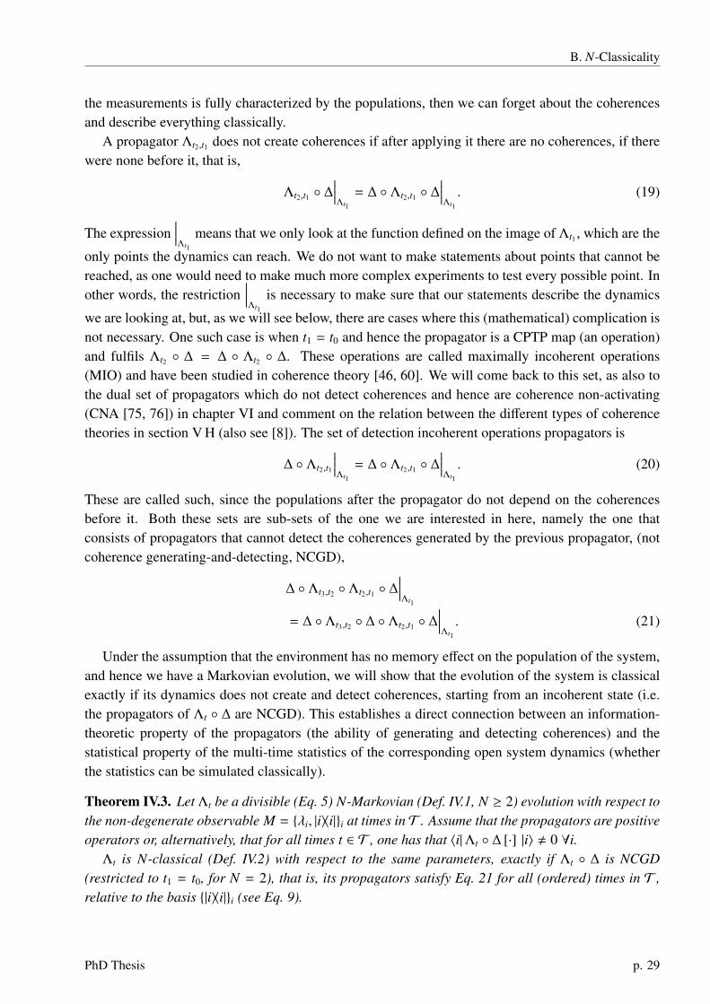
A propagator Λt2,t1 does not create coherences if after applying it there are no coherences, if therewere none before it, that is,

Λt2,t1 ◦ ∆∣∣∣∣Λt1

= ∆ ◦ Λt2,t1 ◦ ∆∣∣∣∣Λt1

. (19)

The expression∣∣∣∣Λt1

means that we only look at the function defined on the image of Λt1 , which are the

only points the dynamics can reach. We do not want to make statements about points that cannot bereached, as one would need to make much more complex experiments to test every possible point. Inother words, the restriction

∣∣∣∣Λt1

is necessary to make sure that our statements describe the dynamics

we are looking at, but, as we will see below, there are cases where this (mathematical) complication isnot necessary. One such case is when t1 = t0 and hence the propagator is a CPTP map (an operation)and fulfils Λt2 ◦ ∆ = ∆ ◦ Λt2 ◦ ∆. These operations are called maximally incoherent operations(MIO) and have been studied in coherence theory [46, 60]. We will come back to this set, as also tothe dual set of propagators which do not detect coherences and hence are coherence non-activating(CNA [75, 76]) in chapter VI and comment on the relation between the different types of coherencetheories in section V H (also see [8]). The set of detection incoherent operations propagators is

∆ ◦ Λt2,t1

∣∣∣∣Λt1

= ∆ ◦ Λt2,t1 ◦ ∆∣∣∣∣Λt1

. (20)

These are called such, since the populations after the propagator do not depend on the coherencesbefore it. Both these sets are sub-sets of the one we are interested in here, namely the one thatconsists of propagators that cannot detect the coherences generated by the previous propagator, (notcoherence generating-and-detecting, NCGD),

∆ ◦ Λt3,t2 ◦ Λt2,t1 ◦ ∆∣∣∣∣Λt1

= ∆ ◦ Λt3,t2 ◦ ∆ ◦ Λt2,t1 ◦ ∆∣∣∣∣Λt1

. (21)

Under the assumption that the environment has no memory effect on the population of the system,and hence we have a Markovian evolution, we will show that the evolution of the system is classicalexactly if its dynamics does not create and detect coherences, starting from an incoherent state (i.e.the propagators of Λt ◦ ∆ are NCGD). This establishes a direct connection between an information-theoretic property of the propagators (the ability of generating and detecting coherences) and thestatistical property of the multi-time statistics of the corresponding open system dynamics (whetherthe statistics can be simulated classically).

Theorem IV.3. Let Λt be a divisible (Eq. 5) N-Markovian (Def. IV.1, N ≥ 2) evolution with respect tothe non-degenerate observable M = {λi, |i〉〈i|}i at times in T . Assume that the propagators are positiveoperators or, alternatively, that for all times t ∈ T , one has that 〈i|Λt ◦ ∆ [·] |i〉 , 0 ∀i.

Λt is N-classical (Def. IV.2) with respect to the same parameters, exactly if Λt ◦ ∆ is NCGD(restricted to t1 = t0, for N = 2), that is, its propagators satisfy Eq. 21 for all (ordered) times in T ,relative to the basis {|i〉〈i|}i (see Eq. 9).

PhD Thesis p. 29

IV. Dynamics

The assumption 〈i|Λt ◦∆ [·] |i〉 , 0 ∀i means that the action of Λt is also invertible as a linear functionon the classical subspace.

Note, that formally we do not need any Markovianity for this theorem to be true, meaning that wewill prove the equivalence between Eqs. 18 and 21 without using that assumption. But if the evolu-tion is not at least N-Markovian, the propagators do not need to be related to the N-times statisticsand hence to the actual evolution if measurements are done (see the discussion around Eq. 6). Inother words, the Markovianity is what connects the statement about the form of propagators to theclassicality of the evolution.

In order to prove this theorem, we need an intermediate step provided by the following lemma. Itstates that NCGD propagators are really those that do not detect the generated coherences.

Lemma IV.4. A divisible evolution is NCGD at times in T exactly if∑j,k

〈l|Λt3,t2[| j〉〈k|

]|l〉〈 j|Λt2,t1 [|i〉〈i|] |k〉 = 0, (22)

for all indices on the initial and final populations i and l, for which 〈i|Λt1 ◦ ∆ [·] |i〉 , 0, and for alltimes t3 ≥ t2 ≥ t1 in T .

Proof. First note that Eq. 22 is satisfied exactly if ∀i, l∑j,k

〈l|Λt3,t2[| j〉〈k|

]|l〉〈 j|Λt2,t1 [|i〉〈i|] |k〉

=∑

j

〈l|Λt3,t2[| j〉〈 j|

]|l〉〈 j|Λt2,t1 [|i〉〈i|] | j〉.

Noting that the left-hand side of this equality is simply 〈l|Λt3,t2[Λt2,t1 [|i〉〈i|]

]|l〉, while the right-hand

side is 〈l|Λt3,t2[∆ ◦ Λt2,t1 [|i〉〈i|]

]|l〉, the lemma follows. �

Proof of Thm. IV.3. We start with the statement that under the given assumptions, if Λt is N-classical,with N ≥ 3, then Λt ◦ ∆ is NCGD. Since Λ is at least 3-classical, we have that∑

i2

Tr[Πi3 ◦ Λt3,t2 ◦ Πi2 ◦ Λt2,t1 ◦ Πi1 ◦ Λt1 ◦ Πi0

]= Tr

[Πi3 ◦ Λt3,t1 ◦ Πi1 ◦ Λt1 ◦ Πi0

]. (23)

Labelling the outcome with |i3〉〈i3|, and remembering the definition of ∆ (Eq. 9), we get, by summingover i3, i1, and i0,

∆ ◦ Λt3,t2 ◦ ∆ ◦ Λt2,t1 ◦ ∆ ◦ Λt1 ◦ ∆

= ∆ ◦ Λt3,t1 ◦ ∆ ◦ Λt1 ◦ ∆, (24)

which is the definition of NCGD for Λt ◦ ∆. The case with N = 2 is exactly the same.The opposite direction follows from IV.4, as detailed below. From IV.4, we have that, by NCGD,

under the assumption that 〈il − 1|Λtl−1 ◦ ∆ [·] |il − 1〉 , 0,∑il, jl

〈il+1|Λtl+1,tl[|il〉〈 jl|

]|il+1〉〈il|Λtl,tl−1 [|il−1〉〈il−1|] | jl〉 = 0


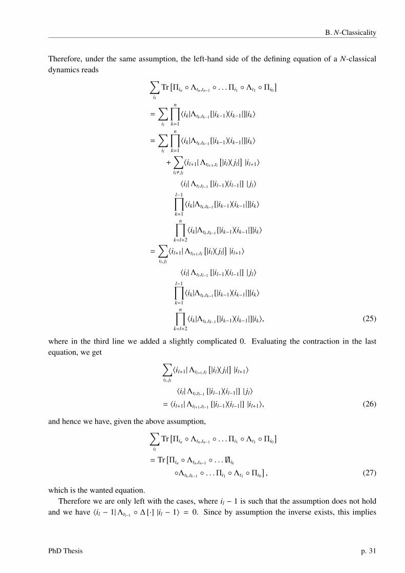
B. N-Classicality

Therefore, under the same assumption, the left-hand side of the defining equation of a N-classicaldynamics reads ∑

il


]=

∑il

n∏k=1

〈ik|Λtk ,tk−1[|ik−1〉〈ik−1|]|ik〉

=∑

il

n∏k=1


+∑il, jl


]|il+1〉

〈il|Λtl,tl−1 [|il−1〉〈il−1|] | jl〉

l−1∏k=1


n∏k=l+2


=∑il, jl


]|il+1〉

〈il|Λtl,tl−1 [|il−1〉〈il−1|] | jl〉

l−1∏k=1


n∏k=l+2

〈ik|Λtk ,tk−1[|ik−1〉〈ik−1|]|ik〉, (25)

where in the third line we added a slightly complicated 0. Evaluating the contraction in the lastequation, we get ∑

il, jl


]|il+1〉

〈il|Λtl,tl−1 [|il−1〉〈il−1|] | jl〉

= 〈il+1|Λtl+1,tl−1 [|il−1〉〈il−1|] |il+1〉, (26)

and hence we have, given the above assumption,∑il


]= Tr

[Πin ◦ Λtn,tn−1 ◦ . . . /Πik

◦Λtk ,tk−1 ◦ . . .Πi1 ◦ Λt1 ◦ Πi0], (27)

which is the wanted equation.Therefore we are only left with the cases, where il − 1 is such that the assumption does not hold

and we have 〈il − 1|Λtl−1 ◦ ∆ [·] |il − 1〉 = 0. Since by assumption the inverse exists, this implies

PhD Thesis p. 31

IV. Dynamics

that Λ−1tl−1

[|il − 1〉〈il − 1|] has zero overlap with the basis |i〉〈i| and the trace is zero. Since Λtl−2 is tracepreserving, we have that Λtl−2 ◦ Λ−1

tl−1[|il − 1〉〈il − 1|] has trace zero. Noting that, by definition,

〈i|Λtl−2 ◦ Λ−1tl−1

[|il − 1〉〈il − 1|] |i〉 = 〈il − 1|Λtl−1 ◦ Λ−1tl−2

[|i〉〈i|] |il − 1〉,

we have that

〈il − 1|Λtl−1 ◦ Λ−1tl−2

∑i

|i〉〈i|

|il − 1〉 = 0

Finally, since by assumption, if 〈il − 1|Λtl−1 ◦ ∆ [·] |il − 1〉 = 0, the propagators are positive, it followsthat all these terms (for any i) must be zero and therefore the left- and the right-hand side of thewanted equation both simplify to 0, and hence are true trivially.

�

2. A philosophical side-note

Note that in classical physics there are processes where the Kolmogorov consistency conditiondoes not hold. This happens if measurements alter some variables which are relevant for the dynamicsin a way that does not cancel out on average. Thinking from a deterministic perspective, one could saythat our measurements simply disturbs some (hidden) variables of the system. This is certainly nottoo wrong, as a measurement will most certainly change the quantum mechanical state of the system(i.e. the quantum mechanical description of the knowledge we have on the state of affairs). However,assuming (as is done for any argument against hidden-variables) that the outcomes of a projectivemeasurements do describe a (composite) state of affairs of the system, the Markov condition saysexactly that this classical state of the system (i.e. the one-time probability) only depends on the lastmeasured state of the system and not on what was measured before. This leaves us with the situationthat the state of the system is always only dependent on the last measured state, while the dynamics isnot determined by the state alone. Again, one can understand this classically, if one assumes that somehidden-variables are changed due to the measurement in a way that will affect the future dynamics,while they do not affect the measurable state directly (for instance, asserting that measuring positionsets the momentum to some given probability distribution, independently of the current momentum orindeed the way one implements the measurement, as long as it is almost instantaneous and projective).Of course, then it seems a bit miraculous that any possible implementation of the same projectivemeasurement affects the dynamics (and hence the hidden variables responsible for the change indynamics) exactly in the same way (that is, hidden variables need to be hidden); if there need to beadditional variables, why can they not be changed in a way that makes them apparent? The argumenthere is that the classical picture is worse than the quantum one for these cases because it needs toassume strictly more, without giving raise to better predictions (similarly as in science one shouldnot assume the existence of intractable elves, even though of course it does not hurt anyone, as, bydefinition, they do not have any measurable influence). This exclusion by Ockham’s razor is of courseless stringent than more direct approaches like the one of Bell [11] or Kochen and Specker [37], eventhough those need additional assumptions.


B. N-Classicality

Indeed one could make the case that any Markovian dynamics is classical in the following way:if at any time the current state of the system completely determines the following dynamics, thereis always at least one rank-1 projective measurement that leaves the state and hence the followingdynamics unaltered, namely measuring in the diagonal basis of the state. Then, there are two types ofvariables one needs to consider, one is the classical probabilities given by the diagonal measurementand the second determines the direction in which one needs to measure. Unfortunately one cannotaccess these second ones directly, in that one can only access the prediction over non-ideal measure-ments, namely disturbing ones. Of course such a theory is highly contextual (as it needs to be) [37]. Inthe case described here, the contextuality consists in that the “correct” way to measure reality dependson some aspects of the actual situation itself.

In any case the aim of this thesis does not concern philosophical issues on quantum mechanics,but the characterization of when a process in a given model can be modelled by a classical stochasticprocess. In this chapter the model consisted of only one given dynamics (coming from a fixed globalunitary) viewed through fixed intermediate measurements. Even so, in the next chapter, while wedo keep an operational approach and the aim is unaltered, we will also find again the familiar resultthat the above interpretation (and, indeed, any hidden variable interpretation) of quantum mechanicsbreaks down, if one assumes locality.

PhD Thesis p. 33

V. COHERENT STATES, ENTANGLEMENT AND QUANTUM DISCORD


After having learned the importance of coherence for the non-classicality of a given dynamics,we look at settings where one has more liberty to act. To simplify our analysis, however, we onlyconsider situations where the actions are given by concatenating or parallel implementationof quantum instruments, that is, standard quantum information scenarios. In this chapter,we use this setting to look more carefully at the creation of entanglement, with the aim ofunifying different types of non-classicality: entanglement, discord, basis-dependent discordand coherence.

This chapter follows closely, often literally, our recent article [5]. This concerns all the sections inthe current chapter where nothing else is stated. Some sections are taken or slightly adapted from apreprint of the article [3]. We state this inside those sections. New are only the parts concerning theconnections with classicality, that is, with Def II.1.

In chapter IV we have seen that we can always see a Markovian dynamics as something classical.In the sense that for any given dynamics that is Markovian relative to a family of non-degenerate ob-servables in the local basis of the system which may only depend on the time (Mt = {λi(t), |i(t)〉〈i(t)|}i),the according multi-time statistics is classical. In this sense, quantum mechanics can always be de-scribed by a classical stochastic Markovian process – given that one considers a large enough statespace. This is due to the fact that if a system is isolated, there is always a rank-one projective mea-surement that does not disturb the system, which, together with the information about what the mea-surement is, fully describes the state (this is nothing than a fancy way to say that every state can bediagonalised). This means that the measurement really behaves like an ideal measurement (also seesection IV B 1). Following this argument, one might believe that the state of a pure system, togetherwith a preferred measurement basis is actually describing the state of affairs of the system. As long asone considers closed (or at least Markovian) systems, this view is consistent. The situation changes ifone adds some additional requirements, such as locality [10].

Locality is the assumption that the state of affairs only changes locally, which implies that an op-eration or a measurement that is performed locally should not alter the state of affairs of a remotesystem [10]. There are two main reasons for this assumption. The more practical one is the believethat nothing travels faster than the speed of light, which serves very well as a foundational principleof special relativity and remains true for how information propagates in quantum physics. The morephilosophical one is that by assuming a non-local reality, one undermines the foundations of exper-imental science, since it is never clear if the outcome of an experiment is due to the experimentalsetting or some unrelated and uncontrollable happenings far away in the universe. While this cannotbe ruled out by logic, it immediately raises the question why the assumptions of isolated systems andrepeatability work so well for physics, and also it takes away at least some of the hope of understand-ing the world, or of the possibility to act independently in it. For a more thorough discussion on thenecessity of locality see e.g. [112]. In any case, this chapter (indeed the full thesis) does not reflect mypreference on this matter (namely that locality is an essential pre-requisite for physics and cannot beeasily dropped without getting into problems with self-consistency), but just characterizes the states

p. 34

that do not lead to a classical local model.A particularly transparent approach to characterize non-classical super-positions, assuming local-

ity, is given by the theory of local operations and classical communication (LOCC) [24, 25], whichexactly incorporates the idea of the impossibility of creating entanglement if one has two distantparties that can only communicate classically.

Q

AQ

B

Communicationthrough a wire

Figure 1. Wires for classical communication are quantum systems. (Figure taken from reference [5]).

However, entanglement is not the only non-classical feature of quantum mechanics. There areother forms of superposition that can also give advantages over classical states. An instance in whichthis became apparent is the protocol of deterministic quantum computation with one qubit (DQC1)that can outperform any known classical algorithms even if no bipartite entanglement is present [33,83, 86, 113, 114]. It was argued that a property denoted as discord [31, 32, 34, 70] would be theresource responsible for this operational advantage. While discord is an interesting measure, it is hardto argue that it is a resource of non-classicality, since it can be created already by mixing discord-freestates (in fact product states) and mixing states amounts to forgetting information – a task that iseasily accomplished classically [32]. Some advances in understanding the resources in DQC1 haverecently been made using a different form of non-classicality, called coherence, which is exhibitedby superpositions of states in a fixed orthonormal basis, whose elements and their statistical mixturesare the incoherent states [8, 45, 46, 60]. Based on this theory, complementing recently studiedconnections between entanglement and coherence [47–49, 79, 89–98], it was shown that the precisionof the DQC1 protocol is a function of the coherence of the qubit one uses as a control and that any statewith some property called basis dependent discord [3, 74, 77–79] is a resource in this setting [3, 74].We will discuss this in more detail in section V F on page 67. We will also see in section V C 2 onpage 58, following our paper [3], that standard (basis independent) measures for discord are recoveredwhen basis dependent discord is minimized over different bases.

However, coherent states and entangled states are inter-convertible resources and optimal instancesof basis dependent discord. There is a certain irony in this, as we set out to find more general resourcesthan entanglement. Even more generally, there is an operation that maps any superposition of agiven set of linearly independent states (not necessarily orthogonal) to entangled states and non-superposition states to separable states [4, 115, 116]. This means that, while entanglement does notseem to be the most generic non-classical resource, as it does not easily encompass all forms of

PhD Thesis p. 35

V. States

superposition that seem useful for quantum tasks, the resources that enable to produce entanglementmight well be the most fundamental form of non-classicality in states. Seemingly, the ability todo something truly quantum entails the possibility to produce entanglement. It is this “universalcharacter" [117] of entanglement, that motivates to have a closer look at that property, as we do inthis chapter.

A. Local operations and physical wires

1. Setting

One of the most successful resource theories in quantum information, and the starting point of ourconsiderations, is the theory of local operations and classical communication (LOCC). This theoryaims to capture the idea of EPR and Bell that in classical physics it is not possible to reproduce theeffect of having non-local superpositions of states [10, 12]. LOCC can be described by its elementaloperations consisting of arbitrary local quantum operations on one system, post-selection and classi-cal broadcasting of the result. Any LOCC operation is a concatenation of such operations (potentiallydepending on the results of the previous ones). Here we want to treat the broadcasting as an operationusing a physical wire, instead of how it is usually done as an implicit exchange of classical informa-tion. The broadcasting is then simply given by forwarding the state of the wire as an ancilla to theparty in question. In this way, it makes sense to talk about the state of the communication channelas a quantum state. Indeed we reverse the usual perspective and instead of only looking at Alice andBob, we focus our attention on the wire.

We strife for a strong definition for non-classical states, meaning, that we only keep states andoperations with a clear classical interpretation (also implying that the model is classical according todefinition II.1). We will also strife for a weak definition of non-classical using definition II.1, withoutfurther assumptions. We will see, however, that there is no gap between the two. Indeed, we will showthat if a state is non-classical (having enough copies of it) one can get whatever statistics allowed byquantum mechanics. We are interested in the classicality of the wire and observe it through a fixednon-degenerate observable, leading to a projective measurement in a pre-selected basis. Henceforthwe will call this basis incoherent and denote it byZ. With this definition, it also makes sense to allowsome classical processing in the wire as a free operation on this extended theory, that is, permutationsof the incoherent basis states. While the basis one uses to encode a probability distribution in the wireis in principle arbitrary, one needs to fix it in advance; to be precise, while the incoherent basis maychange in time, this change must be defined at the beginning of the protocol. To clarify the importanceof fixing the basis in advance (and therefore which states are incoherent) to get a fair description ofthe role coherence plays, we now review the BB84 protocol [26].

The goal of BB84 is to distribute random keys in a safe way. This is achieved by sending qubitsthrough a quantum channel where each of them is encoded by Alice in one of two possible non-commuting bases depending on the outcome of a random measurement. At the other end of thechannel, Bob measures the qubit in a random basis. After repeating this many times, Alice and Bobpublicly compare the bases chosen and keep only the data of the measurements that were done in thesame bases. They can then compare a fraction of the remaining data to be certain (in the asymptotic



limit) that nobody interfered. A naive approach to describe this protocol is that as in each roundthe state of the qubit sent is diagonal in some basis, then the full protocol is classical. How then isit possible that this algorithm beats classical key distribution? The crucial departure from classicalphysics of this protocol is the random choice of bases. The security of the algorithm relies on the factthat the choice of the basis in which the qubits are diagonal is unknown to a possible eavesdropperEve. For her, whatever basis she assumes to be incoherent, there will be some states sent by Alicethat will be coherent, given a long enough sequence. This is the case, because she does not know theoutcomes of Alice’s measurements that defined the encoding bases. For this reason, a fair descriptionof what Eve can do, needs to assume that she chooses the basis before knowing the basis in whichAlice encodes the state. To analyse the security of this protocol, we need to take the perspective ofEve.

Let us resume our discussion above, on the classicality of quantum physics. Alice can simply seethe expected probabilities of a measurement in the basis she encoded the state of the system she sendsto Bob to be a fair description of the state of affairs of that quantum system. This is possible, as sucha measurement only reveals the state without altering it on average. Eve, however, not knowing thebasis in which the state is encoded, is likely to disturb the system if she tries to gain some knowledgeon it. This is the case from the perspective of Alice, even though it is possible for Eve to makea non-disturbing measurement of the system from her own perspective (here, as in many cases inquantum physics, the mixed state of the system depends on who describes it). In this picture Alicemight say that not only Eve does not know the classical state of the system, but not even how todescribe it (classically). Indeed, the only classical description Eve can give that with certainty doesnot conflict with the one of Alice is a trivial one, and, accordingly, from Eve’s perspective, the stateAlice sends in the BB84 protocol is fully mixed. This argument of course is only valid assumingthat there are no hidden variables. If there were, Eve’s lack of knowledge could be interpreted asa classical lack of knowledge on the hidden variables determining the basis in which the state isdiagonal. Furthermore, if these variables were measurable without disturbing the state of the system,the security of the protocol would be compromised. In other words, the security relies on the non-existence of classical (not hidden) variables explaining quantum theory. Note that the above is not anargument against hidden variables, but an explanation why one can have a security advantage, if thefundamental theory is quantum mechanics and not classical physics with hidden variables that whilenot measurable now, in principle would be.

After this excursion on the need for fixing the basis before the protocol for a fair description, wereturn to the discussion of what are the free operations in our generalisation of the setting of LOCC.As noted in the introduction, we only need one quantum system Q together with a wire W to get ameaningful theory. We start by describing this case in some detail, before coming back to the one withmultiple parties Q = ⊗iQi and wires W = ⊗ jW j (and hence really to the setting generalizing LOCC).Even though in this case the wire is really considered to be a classical register, we will continue to usethe word wire throughout for notational ease. In this case, we interpret Alice as an external operator.We give her (a part of) our system and she tells us her outcomes, which we can encode in anotherpart of our system again. From our perspective, the only thing she does is to process, in some wayunknown to us, the random variables describing our system. If this description is valid, the actionof Alice is a stochastic process practically by definition. The only restriction we impose on Alice is

PhD Thesis p. 37

V. States

quantum mechanics.For simplicity, to change the phases of the basis states is also assumed to be a free operation – but

as shown below, this has a negligible effect on the theory (apart from making it more concise). Weassume that both Q and W are finite dimensional systems, but don’t keep their dimensions fixed 6).The free operations in this case consist of iteratively applying the following elemental Kraus opera-tions (which should form a completely positive and trace preserving (CPTP) map on W ⊗ Q, that is∑α Kα†Kα = 1, see Appendix A) and post-selecting (for a neater notation we only write out the spaces

on which the Kraus operations act non-trivially, on all others the identity operation is assumed):

1. Permutations: Permutations σ of basis states in the basisZ on the wire W,∑

i |σ(i)〉〈i|W .

2. Phases: Diagonal unitary evolutions in the basisZ on W,∑

j ei φ( j)| j〉〈 j|W .

3. Observed quantum operations: Any generalized measurements on Q, encoding its outcomesas an incoherent state of an ancillary subsystem Wa of W, |α〉Wa ⊗ Fα

Q, for Kraus operators FαQ

acting on Q.

4. Classical to quantum forwarding: Transfer a subsystem Ws of W to a subsystem Qt of Q:1Qt←Ws =

∑j | j〉Qt〈 j|Ws =

∑j〈 j|Ws ⊗ | j〉Qt .

For simplicity, here we assume the incoherent basis Z to be the same for all times, but one caneasily get the more general setting by replacing the free operations Kα by (UW(t, t0) ⊗ 1Q)Kα, whereUW(t, t0) defines the (necessarily predefined, see above) change of basis for the time-step t0 → t. Notethat this includes replacing the identity by (UW(t, t0)⊗1Q) and that the identity operation itself is not afree operation any more. Sticking to this rule the results stay unchanged, because concatenating freeoperations on t0, t1 and t1, t2 yields free operations on t0, t2. This is relevant if one wants to changethe basis one calls classical in time, as is usually the case in settings where discord is thought to be ameaningful measure. We will come back to this in subsection V D.

Note also that we treat encoding and decoding asymmetrically. An operational reason for thisis that it is hard to encode quantum information in a wire, but if coherence is provided and it ispossible to sustain, transport and control it, you may very well also be able to use it. That is why weonly allow to encode classical information in the wire, while any state can be retrieved. Alternativeinterpretations of the free operations are given in the caption of Fig. 2 and in section V B (see Fig. 4on page 42). We call the set of free operations in this theory of local operations and physical wiresLOP(W ← Q) = LOP, were here we use the symbols ← and → for classical encoding, while fand are used for transferring a quantum system. Items 3. and 4. are depicted in Fig. 2. To geta clearer idea of the operations at hand, we will need to find a more compact form of the operationsbelonging to LOP. To this end and of independent interest it is helpful to know bijections that areelements of LOP. Knowing bijections in a resource theory is useful because they define equivalenceclasses on states: all states that can be reached by bijections can be freely interconverted, makingthem equivalent resources (as for any task one state can be used for, any state that can be mapped

6 For any ancilla W2 to W1 we fix an incoherent basis (| j >W1 , |k >W2 ) and label the full basis of the new W by natural numbers|i >W= |i( j, k) >W . We implicitly use the change of representation |i( j, k) >W≡ | j >W1 ⊗|k >W2 . We also identify c ⊗ |Ψ >= c|Ψ > forscalars c ∈ C throughout, and similarly < j|Ws ⊗ | j >Qt = | j >Qt< j|Ws ; also see Appendix A.



a) b)

Figure 2. The picture depicts items 3. and 4. of the elemental operations defining LOP. Item 3., depicted in sub-figure a),means that to do operations on the quantum state, measure what happens and use the incoherent basis of the wire to encodethe observation is considered to be a classical operation on the wire and therefore free. Item 4, depicted in sub-figure b),means that the wire is effectively treated as a quantum system. This means that it can interact with the quantum systemin a quantum way. However, if the wire is an extended object, it might be hard to change its state in a controlled way bythis interaction. Therefore it is considered a free operation to forward the state of a subsystem of the wire to the quantumside, but the ways to alter the state of the wire are strongly restricted. (Figure taken from the preprint of reference [5]).

into it is at least as useful). A trivial bijection in LOP is given by any unitary on Q, which means thatany measure of the theory necessarily has to be invariant under basis changes of Q. The followinglemma establishes such a bijection between the states on the wire W and maximally correlated stateson W ⊗ Q (also see [47, 92]).

Lemma V.1. The operator B : W → W ⊗ Q, B =∑

i |i〉〈i|W ⊗ |i〉Q defines an injection and definingB[ρ] = (BρB†), B ∈ LOP. Conversely there exists a map B−1 : W ⊗ Q→ W, with B−1 ◦ B = 1W andB−1 ∈ LOP.

Proof. The operator B =∑

i |i〉〈i|W ⊗ |i〉Q can be implemented by a sequence of maps that will bedescribed in the following in terms of their Kraus operators. To this end we start with W = W1 andQ = 1 and apply

1. |0〉W2

2.∑

i, j |i〉〈i|W1 ⊗ |i + j〉〈 j|W2

3.∑

i, j〈 j|W2 ⊗ | j〉Q,

where the first map is a single outcome measurement of Q storing the outcome in an ancilla W2

(observed quantum operation), the second is a permutation on W, and the third is the forwarding ofthe system W2 to Q. Identifying W = W1, we get the desired operation.

For the converse, we first apply a measurement in the Fourier basis, followed by a correction ofthe phase on W.

1. FT k = 〈k|Q =∑d

j=1e2π i k j/d√

d〈 j|Q

2. D(k) =∑d

i=1 |i〉〈i|We−2π i ki/d,

resulting in the action B−1k=

∑di=1

∑dj=1

e2π i k( j−i)/d√

d|i〉〈i|W ⊗ 〈 j|Q. Obviously the map defined by these

Kraus operators is an element of LOP and a left-inverse of B, as required. �

PhD Thesis p. 39

V. States

We conclude this subsection defining LOP with the promised proposition, which states that thephases are not really relevant:

Proposition V.2. Any operation in LOP can be done with arbitrarily high probability of success by acombination of permutations, observed quantum operations and classical to quantum forwarding.

Proof. Let W have dimension d. The only thing to show is that indeed one can change the phaseson W in the above framework. Let U =

∑j ei φ( j)| j〉〈 j|W be the wanted phase shift. Define UQ2 =∑

j ei φ( j)| j〉〈 j|Q2 . We start by identifying Q = Q1. The protocol is:

1. B =∑

i |i〉〈i|W ⊗ |i〉Q2 as in Lem V.1

2. UQ2

3. FT k = 〈k|Q2 =∑d

j=1e2π i k j/d√

d〈 j|Q2 , (1 ≤ k ≤ d)

4. If k = d: stop.

Else: redefine UQ2 = UQ2 ◦∑

j e−2π i k j/d| j〉〈 j|Q2 and restart with item 1.

The probability of success in each round is given by 1/d, independently of the initial state. After Miterations we therefore have a probability of success given by

∑Mi=1 1/d(1−1/d)(i−1) = 1−

(1 − 1

d

)M→ 1

for M → ∞. �

B. Basis dependent discord and coherence

In this subsection we give alternative formulations of the resource theory of LOP, defined in thelast section, deepening its understanding. These formulations will prove useful to connect the theoryto other approaches, such as basis dependent discord and coherence, which are summarized in Fig. 11on page 77. It is easy to see that the set of free states that can be prepared (probabilistically or not) byLOP is given by the so-called incoherent-quantum states, CQ(n)

Z= {ρ | ρ =

∑m pm|m〉〈m|W⊗σmQ, |m〉 ∈

Z} [47, 74]. Therefore LOP is a subset of the incoherent-quantum operations (IQO), that is given byany operations that map incoherent-quantum states to incoherent-quantum states, even after post-selection [74]. It is not so easy to see how strict the inclusion is. We will discuss this question later inProp. V.6 on page 46, once we have gathered more insight into the theory.

We start by giving an equivalent characterization of the operations in LOP, which has the advantageof being an explicitly finite concatenation of maps of one fixed form. This is a bit technical and mightbe omitted in a first reading (just skip this paragraph, Prop. V.6 and Fig. 3 and continue with the nextparagraph on page 42), but it is also a useful and non-trivial result. On one hand, a finite form mighthelp to find a minimal number of Kraus operators [118] necessary to represent a deterministic LOPoperation, on the other, a priori it is not obvious that such a simplification exists, since for LOCC,which is a very similar theory, the number of rounds needed for a transformation is unbounded [119].The proposition states that one can write any element of LOP as a concatenation of N LOP maps (andN is bounded by the Hilbert space dimension of the wire) that are composed of Kraus operators Kα j

j

having a specific functional form. Due to the possibility of post-selection, one has to consider different



paths given by the outcomes of the generalized measurements, that is, which Kraus operators Kα j

j havebeen measured; after t maps (labelled from 1 to t), these paths are denoted by ~αt, and αt+1 denotesthe possible outcomes of the map labelled by t + 1. Both the maps and the length of the protocolmay vary depending on the outcomes of previous measurements, but for any path ~α, the total lengthN = N(~α) can be restricted to be less or equal to the dimension of the Hilbert space of the wire. Thisfiniteness of the protocol is proven by showing that one can find a protocol that bounds the supporton the wire of each branch ~αN , in each step t, by a monotonically decreasing sequence of integersr(~αt−1). Fig. 3 depicts a generic example for a protocol which acts on an initially three-dimensionalwire and a quantum system.

Figure 3. The figure shows a diagram for a possible protocol defining an LOP map as described in Prop. V.3. In thisexample the input state is three-dimensional on the wire. All the arrows starting from the same node represent a CPTPmap. Each arrow represents a sub-map with a given outcome (labelled from 1 on the left to n on the right). The dimensionof the maximal support of the input or output states on the wire is stated on the left of the diagram. The branches canbe grouped into four different types, where the types differ by how the dimension of the maximal support of the state onthe wire (given wlog by r(~αt−1), after applying t maps with the outcomes ~αt), changes during the protocol. Any possiblebranch type is depicted at least once. In this picture the respective groups of outcomes for the four branch types are (weonly name the outcome vectors up to the point that the group is defined): {(1), (2)}, {(3), (4), (5)}, {(6, 1)} and {(6, 2), (7)}.See the Appendix for more details on the branch types. The highlighted branch is given by Λ2(2) ◦ Λ2

1, that is, the CPTPmap Λ2(2) = Λ1

2(2) + Λ22(2) (composed by two sub-maps), after getting the outcome 2 in the first map. The length of the

protocol N is 2 for these outcomes, while it is 3 for e.g. the outcomes (7,2). In principle the dimension of the supportof the outcome state on the wire after applying an LOP map is arbitrary (though for the depicted protocol it is at most3 × 3 + 1 × 2 + 7 × 1 = 18). (Figure taken from reference [5]).

Proposition V.3. Let us denote by Λ1 a selective CPTP map with outcomes α1 represented by Krausoperators Kα1

1 . Depending on the obtained outcome α1, we define the next selective CPTP map Λ2(α1),with outcomes α2, represented by Kraus operators Kα2

2 (α1). In the same way, we define Λt(~αt−1),which depends on the outcomes of all previous maps through ~αt−1 = (α1, . . . αt−1). For notationalconvenience, we define ~α0 = ~α−1 = 0.

Let Λ be a CPTP map acting on W ⊗Q. Then Λ is an LOP operation exactly if it can be written as

Λ = ΛN(~αN−1) ◦ . . . ◦ Λ2(α1) ◦ Λ1, (28)

with

Kαtt (~αt−1) =

r(~αt−2)∑i=1

|σ~αt ◦min[r(~αt−1), i]〉〈i|W ⊗ Eαtt

(~αt−1, i

), (29)

PhD Thesis p. 41

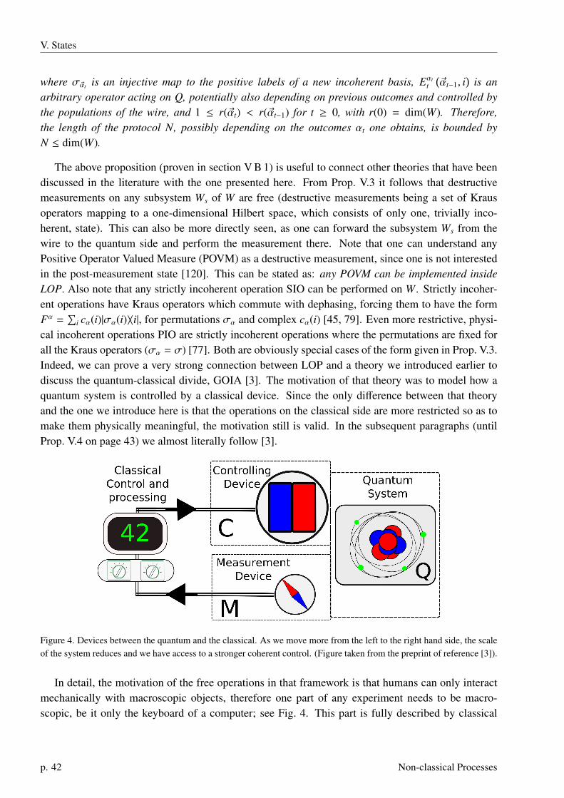
V. States

where σ~αt is an injective map to the positive labels of a new incoherent basis, Eαtt

(~αt−1, i

)is an

arbitrary operator acting on Q, potentially also depending on previous outcomes and controlled bythe populations of the wire, and 1 ≤ r(~αt) < r(~αt−1) for t ≥ 0, with r(0) = dim(W). Therefore,the length of the protocol N, possibly depending on the outcomes αt one obtains, is bounded byN ≤ dim(W).

The above proposition (proven in section V B 1) is useful to connect other theories that have beendiscussed in the literature with the one presented here. From Prop. V.3 it follows that destructivemeasurements on any subsystem Ws of W are free (destructive measurements being a set of Krausoperators mapping to a one-dimensional Hilbert space, which consists of only one, trivially inco-herent, state). This can also be more directly seen, as one can forward the subsystem Ws from thewire to the quantum side and perform the measurement there. Note that one can understand anyPositive Operator Valued Measure (POVM) as a destructive measurement, since one is not interestedin the post-measurement state [120]. This can be stated as: any POVM can be implemented insideLOP. Also note that any strictly incoherent operation SIO can be performed on W. Strictly incoher-ent operations have Kraus operators which commute with dephasing, forcing them to have the formFα =

∑i cα(i)|σα(i)〉〈i|, for permutations σα and complex cα(i) [45, 79]. Even more restrictive, physi-

cal incoherent operations PIO are strictly incoherent operations where the permutations are fixed forall the Kraus operators (σα = σ) [77]. Both are obviously special cases of the form given in Prop. V.3.Indeed, we can prove a very strong connection between LOP and a theory we introduced earlier todiscuss the quantum-classical divide, GOIA [3]. The motivation of that theory was to model how aquantum system is controlled by a classical device. Since the only difference between that theoryand the one we introduce here is that the operations on the classical side are more restricted so as tomake them physically meaningful, the motivation still is valid. In the subsequent paragraphs (untilProp. V.4 on page 43) we almost literally follow [3].

Controlling

Device

C

MFigure 4. Devices between the quantum and the classical. As we move more from the left to the right hand side, the scaleof the system reduces and we have access to a stronger coherent control. (Figure taken from the preprint of reference [3]).

In detail, the motivation of the free operations in that framework is that humans can only interactmechanically with macroscopic objects, therefore one part of any experiment needs to be macro-scopic, be it only the keyboard of a computer; see Fig. 4. This part is fully described by classical



physics. To model this in quantum mechanics, following [8] we say that the state of a system is inco-herent (or classical, though this is less precise, see e.g. [4]) if it is diagonal in a fixed basis. Secondly,there are some experimental devices which allow us to operate on the full quantum system. These in-termediary devices are usually in the mesoscopic domain, since we want to manipulate their operatingparameters in a deterministic way and, at the same time, use them to manipulate microscopic quantumsystems. Because of their size it is an operationally hard task to bring these devices controllably intoa coherent superposition that remains stable against decoherence. In order to cast this situation into aresource theory perspective, it is advantageous to assume that only incoherent operations are availableand all required coherence is supplied by a third party. For this reason, we might think of coherenceas a resource for the manipulation of the controlling devices. Following [8], we thus define:

Definition V.1. We call a quantum operation incoherent if each of its Kraus operators Kα is incoher-ent. That is, for any σ incoherent, KασKα

† is incoherent.

We want to use these intermediary devices to control a quantum system, and in the best case,we can have perfect quantum control. We must keep in mind that the controlling devices decoherequickly due to their size. Therefore it might be hard to encode information in a control basis whichis not the incoherent one and still have a stable quantum control. The best stable control we can hopefor is therefore given by the unitary

Ucontrol =∑

m

|m〉〈m|control ⊗ Utarget(m) (30)

We also assume that we can add ancillae to the quantum system and that we can trace out parts of thesystem, i.e. we can prepare and discard parts of it.

Ultimately we might wish to measure the quantum system. We therefore include a measurementdevice, which couples to the quantum system, performs any measurement of the quantum system, andsends the classical measurement result to a computer. This is described by

ρ 7→∑α

|α〉〈α|control ⊗ KαρKα† (31)

where the left-hand side of the tensor product denotes a register in the computer’s memory and theright hand side is the state of the quantum system. Replacing the incoherent operations above, by theslightly more restrictive class SIO, we get that this theory is equivalent to LOP. We will see below thatalso without the replacement the theories are almost the same. We see that from this more operationalpoint of view the zoo of different coherence theories (see section V H on page 77) gets simpler, which,I would argue, makes the interpretation more transparent. From here on I follow again ref. [5].

Proposition V.4 (SIO, PIO and LOP). Let Λ be a CPTP map acting on W⊗Q. Λ is an LOP operationexactly if it can be written as a sequence of maps Λ = ΛM(~αM−1) ◦ . . . ◦ Λ1, for some finite M, whereeach Λi is

(a) a physical incoherent operation on W

or (b) a destructive measurement in one fully coherent basis of a subsystem of W

or (c) a controlled unitary (Ucontrol =∑

m |m〉〈m|control ⊗ Utarget(m)) with control W and target Q

PhD Thesis p. 43

V. States

or (d) a generalized measurement of Q, encoding the result on W (ρ 7→∑α|α〉〈α|W ⊗ KαρKα†).

One can equivalently replace the item (a) by “a strictly incoherent operation on W” or “permutationsand phases on W”.

Proof. We start the proof by noting that any destructive measurements on a subsystem of W can bedone by LOP operations by classical to quantum forwarding of the subsystem in question to an ancillain Q, Q2, and then doing the measurement there. Strictly incoherent operations are those with a Krausdecomposition with Kraus operators of the form Kα1 =

∑di=1 c(α)|σα(i)〉〈i| [45], which obviously is a

special case of the form K1 in Prop. V.3 (i.e. Eq. 29), the same is true for control unitaries of the form(c). Next we note that PIO is a subset of SIO [77], so that any operation having a decomposition as inthe proposition is an element of LOP.

For the converse we only need to show that we can do classical to quantum forwarding using onlythe operations (a)-(d). This goes by virtually the same protocol we already applied for the inverse partof Lem. V.1. We first do a controlled unitary from the system Ws in question to an ancillary systemQs prepared in the state |0〉, to which we want to teleport, apply a measurement in the Fourier basis ofWs (note that measurements in different fully coherent bases only differ by a diagonal unitary, whichis an element of PIO, so we can assume wlog that the basis we can measure in is given by the Fourierbasis), followed by a correction of the phase on Qs:

1. |0〉Qs

2.∑

i |i〉〈i|Ws ⊗∑

j |i ⊕ j〉〈 j|Qs

3. FT kWs

= 〈k|Ws =∑dim(Ws)

j=1e2π i k j/ dim(Ws)√

dim(Ws)〈 j|Ws

4. D(k) =∑dim(Ws)

l=1 |l〉〈l|Qse−2π i kl/ dim(Ws),

resulting in the action∑

i〈i|Ws ⊗ |i〉Qs . �

Noting that items (a), (c) and (d) together form an effective theory of the strictly incoherent oper-ations by restricting the theory to the effect on the wire [79], we find that the present approach (apartfrom giving a completely different motivation) only differs by allowing more general measurements.This difference however, is crucial; that strictly incoherent operations commute with dephasing meansthat apart from being unable to create coherences, they affect populations only depending on popu-lations, making them incoherent in a very strict sense. So strict, in fact, that coherences do not haveany effect that can be measured by free operations. This means that coherences are useless for anyobservable task in that resource theory and hence there are no resource states in the theory. In con-trast, one would expect that a meaningful resource helps to overcome the restriction imposed by theresource theory. Only if this is the case, the questions of how much resources one needs for a giventask makes sense (while water does cost something and in some situations is very useful, it does nothelp you if you want your engine to run and hence is not the relevant resource for transport). Ide-ally, but maybe not always necessarily, one would find that having enough non-free states at handremoves completely any restrictions of the theory. Exactly this we find in the present approach: ifsupplemented by enough coherent ancillary states, LOP can be used to achieve any desired quantumoperation.



Theorem V.5 (Resource states). Let Λ be a CPTP map acting on W1 ⊗ Q, with W1 having dimensiond. Let |ψ〉 =

∑di=1

1√

d|i〉 be a maximally coherent state on W2. Then there is an operation Λ′ ∈

LOP(W2 ⊗W1 ← Q), with TrW2[Λ′[|ψ〉〈ψ|W2 ⊗ ρW1,Q]] = Λ[ρW1,Q].

Proof. The trick is to do the operation on the quantum side, that is: send the system W1 to Q2, do theoperation Λ on Q2,Q1. Then use Lem. V.1 to construct a Bell-type state from the ancillary coherentstate on W2. Finally teleport the system Q2 back to W1 using the original teleportation protocol [121]and using up the ancillary Bell state. In detail (identifying Q1 = Q at the beginning and at the end):

1. Preparation: |ψ〉W2 ,

2. (free) teleportation to the quantum side∑

i〈i|W1 ⊗ |i〉Q2 ,

3. Application of Λ on the quantum side: ΛQ2,Q1 ,

4. Doubling of W2 (Lem. V.1):∑

i |i〉〈i|W2 ⊗ |i〉Q3 ,

5. Measurement in the ‘Bell basis’ 〈b(k, l)|Q3,Q2 , given by |b(k, l)〉 = CNOT ◦ (|k〉 ⊗ |l〉) =

1/√

d∑

j e2π i k j/d| j〉 ⊗ |l ⊕ ( j − 1)〉, with a ⊕ b = mod d(a + b − 1) + 1,

6. Finish with a diagonal unitary∑

j e2π i k j/d| j〉〈 j|W2 on W2 followed by a permutation∑

j |l ⊕ ( j −1)〉W1〈 j|W2 , both depending on the d2 possible outcomes of the previous measurement, given bythe indices k, l.

Using the Kraus decomposition for the map Λ(ρ) =∑α KαρKα†, we get that the full protocol is given

by the (d2) Kraus operators∑z

|l ⊕ (z − 1)〉W1〈z|W2 ◦∑

c

e2π i kc/d|c〉〈c|W2

◦ 1/√

d∑

a

e−2π i ka/d〈a|Q3 ⊗ 〈l ⊕ (a − 1)|Q2

◦∑

j

| j〉〈 j|W2 ⊗ | j〉Q3

◦ KαQ2,Q1

◦∑

i

〈i|W1 ⊗ |i〉Q2

◦

d∑t=1

1√

d|t〉W2

=1d

∑i, j

|l ⊕ ( j − 1)〉〈i|W1

⊗((〈l ⊕ ( j − 1)|Q2 ⊗ 1Q1) ◦ Kα

Q2,Q1◦ (|i〉Q2 ⊗ 1Q1)

)=

1d

KαW1,Q1

,

using that only the terms with z = c = j = a = t survive. �

PhD Thesis p. 45

V. States

We conclude that coherence is a meaningful resource in LOP. Furthermore, from Lem. V.1 itfollows that the resource of coherence

∑di=1

1√

d|i〉W can be reversibly converted into entanglement

between the wire and the system Q,∑d

i=11√

d|ii〉WQ which hence is an equivalent resource of the theory

(also see [3, 47]). Note that the wire and the quantum systems are not spatially separated. Thereforethe interpretation of entanglement as non-classical correlation over a distance – as it arises naturallyin the LOCC setting – is less fruitful. One may then wonder what entanglement between the wireand the system Q means and which implications it my have. As a reminder, let us first look moreclosely at the interpretation of entanglement in the case of LOCC. If the system is in a maximallyentangled state, quantum mechanics predicts strong correlations between different sets of possiblelocal measurement outcomes. These correlations can relate in a way that is not possible classically(in a local hidden-variable theory), due to the distance of the parties [14]. In LOCC one assumes to beable to keep, measure and manipulate the state locally and coordinate the manipulations by classicalcommunication (these are the free operations). Therefore entanglement between two distant partiesgives an upper bound to the ability of using and manipulating non-classical correlations. On the otherhand, for entanglement between a quantum system and a wire in LOP, we are more restricted in themanipulation. Instead, the wire is thought to be an extended system and is connected to the quantumsystem over which one has full quantum control. So that in this case the entanglement gives a boundto the ability to spread and measure the strong correlations, and by doing so, making them provablynon-classical. Additionally, one can use any resource state to coherently control the wire [3], and forinstance steer its state [92]. In section V E on page 64, we will give more details on the connectionbetween classicality on the wire and resource states.

The above properties resemble much those found for incoherent-quantum operations (IQO) [74]and as stated above, the free operations of this theory contain LOP. But how strict is this inclusion?In the following proposition (which we prove in sections V B 1 and V B 3), we show that in generalincoherent-quantum operations cannot be performed by LOP operations. However, we also show thatthey are related.

Proposition V.6 (LOP and IQO). Let Λ be an incoherent-quantum operation on W1 ⊗ Q, whichis exactly the case if it is CPTP and has a Kraus decomposition with Kraus operators of the formKα =

∑i | fα(i)〉〈i|W1 ⊗ Eα(i), for some functions fα acting on the labels of the incoherent basis and

some operators Eα(i) acting on Q. Let d := dim(W1). If d = 2, Λ ∈ LOP. For d ≥ 3 LOP, IQO, butthere is a stochastic implementation of the map in LOP with a success rate of at least 1/d; i.e. thereis an operation Λ′ ∈ LOP(W2 ⊗W1 ← Q) with Λ′[|0〉〈0|W2 ⊗ ρ] = |0〉〈0|W2 ⊗ Λ′0[ρ] + |1〉〈1|W2 ⊗ Λ′1[ρ]with Λ′1[ρ] = Λ[ρ]/d ∀ρ.

Meaning that even though the theories LOP and IQO differ, they are very similar (see the proofin section V B 1 on page 52). Equally close are the theories they induce on the wire (by tracing outQ at the end). We conclude that the effective theory we obtain by restricting LOP to the wire –even though being operationally motivated – is in many aspects similar to the abstractly motivatedtheory of coherence introduced in [8], were the free operations are any that can be decomposed intoKraus operators that cannot create coherence. Specifically, the free states are the same, the resourcestates are the same and the same amount of resources is needed to remove all restrictions of thetheories, in both theories any destructive measurements can be performed, for qubits the theories are



equivalent and for higher dimensions the theories are stochastically equivalent. Up to now LOP isthe only theory that at the same time has a clean operational interpretation in terms of being givenby meaningful elemental operations, while also having resource states that really are resources of thetheory (see the argument above on page 44). The strong connection to IO [8], also gives some moreweight to that theory, which, while the operations do not have such a striking motivation, can be givenin terms of Kraus operations of a much simpler form [45]. We give some more details on the differenttheories of coherence and entanglement in section V H. In the next section we will use the connectionsbetween different theories derived here to provide lower and upper bounds on operationally motivatedmeasures of coherence.

In the next subsection we give the proofs of Prop. V.3, and Prop. V.6 on page 52. The explicitform of LOP for a three-dimensional wire is given in subsection V B 2 on page 54. This is thenused to construct an explicit counterexample, showing that LOP is not the same theory as IQO, ifthe dimension of the wire is greater than two in subsection V B 3 on page 55. We continue with lesstechnical aspects of the theory in section V C on page 56.

1. Proofs

The next two pages are devoted to the proof of the closed form of LOP operations, which simplifiesits use for both theoretical as well as practical purposes, for instance for the comparison of LOP toother resource theories. We then use this result to prove the connection between LOP and IQO.

One of the non-trivial results that we need to show in the proof of Prop. V.3 is that classicalto quantum forward can indeed be decomposed as described in the proposition. In the followinglemma we slightly generalize this statement, as it does not significantly complicate the proof and thestatement might be of independent interest.

Lemma V.7. Let Λ =∑α Fα · Fα† be a CPTP map acting on both W and Q with

Fα =

d∑i=1

| f (i)〉〈i|W ⊗ EαQ(i), (32)

where f maps indices to indices. Then Λ admits a decomposition as in Prop. V.3.

Proof. For simplicity, we will only prove that there is a finite protocol of the given form. That thelength of the protocol is bounded by the dimension of W will be proven independently later in theproof of Prop V.3. The function f in Eq. 32 can map different members of the incoherent basis tothe same output state. The main idea of the proof is to first reorder the incoherent basis of the wire(using a bijection) in such a way, that we can then use a sequence of maps with Kraus operators ofthe form Eq. 29 to implement the same map and the same sub-selection possibilities as with the givenoperators 32. The main trick is to iteratively collapse the subspaces belonging to the pre-image of| f (i)〉.

Let us begin with the case that the image of f (i) is {1, . . . s} for a s ∈ N ≤ dim(W). DefineWk = {i | f (i) = k} and a permutation σ1 that maps the elements of Wk to {1+

∑k−1j=1 |W j|, . . . ,

∑kj=1 |W j|}.

This implements the announced reordering of the incoherent basis of the wire and corresponds to

PhD Thesis p. 47

V. States

a unitary Λ1 given by K1 = |σ1(i)〉〈i|W . Next we define rt = t +∑s−t

j=1 |W j|, e.g. r0 = dim(W),r1 = 1 +

∑s−1j=1 |W j|, rs−1 = s − 1 + |W1| and rs = s. With this, we then define (for t ∈ {2, . . . s + 1})

Kαtt =

rt−2∑i=1

|σrt−1⊕ ◦min[rt−1, i]〉〈i|W ⊗

EαtQ1

(i) ⊗ |αt〉Q2 , i ≥ rt−1

1Q1 , i < rt−1(33)

where the permutation σl⊕ is defined by the mapping i 7→ i + 1, for i < l and l 7→ 1. These Kraus

operators are of the form given in Eq. 29.From the CPTP condition for the Kraus operators defined in Eq. 32, we get that

∑i, j∈Wk

|i〉〈 j|W ⊗∑α Eα

Q(i)†EαQ( j) =

∑i∈Wk|i〉〈i|W ⊗

∑α Eα

Q(i)†EαQ(i) = 1. This implies that for each t ∈ {2, . . . s + 1}, Kαt

t

are Kraus operator of a CPTP map, that is∑αt

Kαtt†Kαt

t = 1.It is straightforward to see by induction that

Kαtt ◦ . . . ◦ K1 =

∑i∈Ws−t+2

|1〉〈i|W ⊗ EαtQ1

(i) ⊗ |αt〉Q2

+∑

i∈Ws−t+3

|2〉〈i|W ⊗ Eαt−1Q1

(i) ⊗ |αt−1〉Q2

+ . . .

+∑i∈Ws

|t − 1〉〈i|W ⊗ Eα2Q1

(i) ⊗ |α2〉Q2

+∑

i∈⋃s−t+1

j=1 Ws

|σ1(i)〉〈i|W ⊗ 1Q

=

t∑u=2

∑i∈Ws−t+u

|u − 1〉〈i|W ⊗ Eαt+2−uQ1

(i) ⊗ |αt+2−u〉

+∑

i∈⋃s−t+1

j=1 Ws

|σ1(i)〉〈i|W ⊗ 1Q

Now we redefine the map Λs+1 → TrQ2 Λs+1, from which follows the statement in the case that theimage of f (i) is {1, . . . s} for a s ∈ N ≤ dim(W). Now assume that the image of f is not {1, . . . s}. Inthis case, we can proceed in the same way and apply a permutation to the image of Λs+1 (before wetrace out Q2) such that we implement the correct f . �

We are now ready to give the proof of Prop. V.3.

Proposition (V.3). Let us denote by Λ1 a selective CPTP map with outcomes α1 represented byKraus operators Kα1

1 . Depending on the obtained outcome α1, we define the next selective CPTPmap Λ2(α1), with outcomes α2, represented by Kraus operators Kα2

2 (α1). In the same way, we defineΛt(~αt−1), which depends on the outcomes of all previous maps through ~αt−1 = (α1, . . . αt−1). Fornotational convenience, we define ~α0 = ~α−1 = 0.

Let Λ be a CPTP map acting on W ⊗Q. Then Λ is an LOP operation exactly if it can be written as

Λ = ΛN(~αN−1) ◦ . . . ◦ Λ2(α1) ◦ Λ1, (34)



with

Kαtt (~αt−1) =

r(~αt−2)∑i=1

|σ~αt ◦min[r(~αt−1), i]〉〈i|W ⊗ Eαtt

(~αt−1, i

), (35)

where σ~αt is an injective map to the positive labels of a new incoherent basis, Eαtt

(~αt−1, i

)is an

arbitrary operator acting on Q, potentially also depending on previous outcomes and controlled bythe populations of the wire, and 1 ≤ r(~αt) < r(~αt−1) for t ≥ 0, with r(0) = dim(W). Therefore,the length of the protocol N, possibly depending on the outcomes αt one obtains, is bounded byN ≤ dim(W).

Proof of Prop. V.3. We need to prove four statements:

1. Any elemental LOP map can be decomposed into an arbitrarily long sequence of CPTP mapsrepresented by Kraus operators of the form given in Eq. 35.

2. Any CPTP map given by Kraus operators as in Eq. 35 can be decomposed as an LOP map.

3. Induction +1: The composition of two CPTP maps that can be decomposed into an arbitrarylong sequence of CPTP maps represented by Kraus operators of the form given in Eq. 35 canagain be decomposed into this form. This statement is trivial.

4. Any CPTP map that can be decomposed into an arbitrary long sequence of CPTP maps rep-resented by Kraus operators of the form given in Eq. 35 can also be decomposed into sucha sequence with r(~αt+1) < r(~αt). From this follows that the choice N ≤ dim(W) is alwayspossible, since r(0) is wlog equal to dim W.

The first statement is easy to see; permutations of the basis Z of W, diagonal unitaries on W, andobserved quantum operations on Q all have the form of Kα1

1 . That classical to quantum forwardinghas the form 35 is a direct corollary of Lem. V.7.

To implement a map given by Kraus operators of the form 35 by elemental operations, the firststep is to implement the trivial observed quantum operation

|0〉W2 ,

followed by a permutation on W given by

r(~αt−2)∑i=1

|min[r(~αt−1), i]〉〈i|W1 ⊗ |i〉〈0|W2 .

Then we do a classical to quantum forwarding of system W2 to an ancillary system Q2. Up to here wecan summarize the concatenation of these operations by

r(~αt−2)∑i=1

|min[r(~αt−1), i]〉〈i|W1 ⊗ 1Q1 ⊗ |i〉Q2 .

PhD Thesis p. 49

V. States

The next step is a quantum operation on Q defined by the Kraus operators

r(~αt−2)∑i=1

Eαtt

(~αt−1, i

)Q1⊗ |σ~αt ◦min[r(~αt−1), i]〉〈i|Q2 ,

which is a quantum operation exactly if the Kraus operators Kαtt (~αt−1) form one. In total, we then have

r(~αt−2)∑i=1

|min[r(~αt−1), i]〉〈i|W1 ⊗ Eαtt

(~αt−1, i

)Q1⊗ |σ~αt ◦min[r(~αt−1), i]〉Q2 .

After a permutation on W1 that implements σ~αt , we obtain in total

r(~αt−2)∑i=1

|σ~αt ◦min[r(~αt−1), i]〉〈i|W1 ⊗ Eαtt

(~αt−1, i

)Q1

⊗|σ~αt ◦min[r(~αt−1), i]〉Q2 .

The last step is to use the operation B−1W1,Q2

from Lem. V.1 to get rid of Q2 and we end up with thewanted operation.

As already mentioned, the third statement is trivial. The hard part is the fourth statement. Assumewe have two arbitrary sets of Kraus operators Kαt

t , Kαt−1t−1 of the given form corresponding to Λt and

Λt−1. Then we distinguish two cases. In the first case, we show that we can find two new sets of Krausoperators Lαt

t , Lαt−1t−1 of the required form such that Kαt

t ◦ Kαt−1t−1 = Lαt

t ◦ Lαt−1t−1 , r(~αt−2) remains the same

and r(~αt−1) < r(~αt−2) for the two new sets (the place where one cuts the Hilbert space dimension ofthe wire in the step t (r(~αt−1)) depends on the previous outcomes, but not on the current one. That iswhy its index is t−1 and not t). In the second case, one can replace the two CPTP maps by one CPTPmap of the required form such that r(αt−2) remains unchanged.

Assume r(~αt−1) ≥ r(~αt−2) (otherwise there is nothing to show). First we split up the injectionσ~αt−1(i) into a permutation and an order-preserving injection. Formally, we define the permutationη~αt−1 on {1, . . . r(~αt−2)} and the injection a : {1, . . . r(~αt−2)} → σ~αt−1({1, . . . r(~αt−2)}) ⊂ N>0 such that

σ~αt−1(i) = a(η~αt−1(i)),

and a(i) < a( j) for i < j. Then there is some l ≤ r(~αt−2) such that

min[r(~αt−1), ·] ◦ σ~αt−1({1, . . . r(~αt−2)}) = {a(1), . . . a(l)}

and

min[r(~αt−1), ·] ◦ σ~αt−1 = min[r(~αt−1), ·] ◦ a ◦ η~αt−1 = a ◦min[l, ·] ◦ η~αt−1 ,

with f (x, ·) denoting the function f (x, y) for fixed x, as a function of y and we use f (A) for a functionf and a set A to denote the image of the set A under f .

We first consider the case l < r(~αt−2). We first define

Fαtt (~αt−1, i) = Eαt

t (~αt−1, σ~αt−1 ◦ η−1~αt−1

(i)) = Eαt+1t (~αt, a(i)),



with i ∈ {1, . . . r(~αt−2)}. By further defining the injection η~αt(k) = σ~αt(a(k)), we can finally define:

Lαtt (~αt−1) =

r(~αt−2)∑i=1

|η~αt ◦min[l, i]〉〈i|W ⊗ Fαtt (~αt−1, i)

and

Lαt−1t−1 (~αt−2) =

r(~αt−3)∑i=1

|η~αt−1 ◦min[r(~αt−2), i]〉〈i|W ⊗ Eαt−1t−1 (~αt−2, i).

First we note that the map defined by Lαt−1t−1 (~αt−2) is CPTP exactly if the map defined by Kαt−1

t−1 (~αt−2) is(as they only differ by a permutation at the end).

Now we show that Lαtt (~αt−1) forms a CPTP map as well. Remember that min[r(~αt−1), a(·)] =

a(min[l, ·]) and since a is a bijection on its image, 〈min[r(~αt), a(i)]|min[r(~αt), a( j)]〉 = 〈min[l, i]|min[l, j]〉.Then

1 =∑αt

Kαtt (~αt−1)†Kαt

t (~αt−1)

⇔∀i, j :

1δi, j = (〈i|W ⊗ 1Q)

∑αt

Kαtt (~αt−1)†Kαt

t (~αt−1)

(| j〉W ⊗ 1Q)

=∑αt

〈min[r(~αt−1), i]|min[r(~αt−1), j]〉Eαtt (~αt−1, i)†E

αtt (~αt−1, j)

⇔∀i, j :

1δi, j =∑αt

〈min[r(~αt), a(i)]|min[r(~αt), a( j)]〉

Eαtt (~αt−1, a(i))†Eαt

t (~αt−1, a( j))

=∑αt

〈min[l, i]|min[l, j]〉Fαtt (~αt−1, i)†F

αtt (~αt−1, j)

⇔1 =∑αt

Lαtt (~αt−1)†Lαt

t (~αt−1).

where we used in the last line that η~αt is a bijection as well.Finally we need to check that we get indeed the right mapping (Kαt

t (~αt−1)◦Kαt−1t−1 (~αt−2) = Lαt

t (~αt−1)◦Lαt−1

t−1 (~αt−2)). This follows from the equalities

r(~αt−2)∑i=1

(|σ~αt ◦min[r(~αt−1), i]〉〈i| ◦ |σ~αt−1( j)〉

)⊗

(Eαt

t (~αt−1, i) ◦ Eαt−1t−1 (~αt−2, j)

)= |σ~αt ◦min[r(~αt−1), σ~αt−1( j)]〉 ⊗

(Eαt

t (~αt−1, σ~αt−1( j)) ◦ Eαt−1t−1 (~αt−2, j)

)= |σ~αt ◦ a ◦min[l, η~αt( j)]〉 ⊗

(Eαt

t (~αt−1, a(η~αt−1( j))) ◦ Eαt−1t−1 (~αt−2, j)

)= |η~αt ◦min[l, η~αt−1( j)]〉 ⊗

(Fαt

t (~αt−1, η~αt−1( j)) ◦ Eαt−1t−1 (~αt−2, j)

)=

r(~αt−2)∑i=1

(|η~αt ◦min[l, i]〉〈i| ◦ |η~αt−1( j)〉

)⊗

(Fαt

t (~αt−1, i) ◦ Eαt−1t−1 (~αt−2, j)

).

PhD Thesis p. 51

V. States

The case l = r(~αt−1) can be handled similarly, just by noting that the action of min[l, ·] gets trivial andone can therefore express the concatenation of the two maps as a single map of the same form.

This proves that one can chose r such, that: dim W ≥ r(0) > r(~α1) > . . . > r(~αN−1) ≥ 1. It followsthat it is always possible to have N ≤ dim W. �

The most general set of meaningful operations, if one just has the restriction that one wants tokeep the wire incoherent and classically correlated with the quantum system, are the operations thatdo not allow to generate states which are not incoherent-quantum from those that are. If one allowspost-selection this means that the same should be true for each Kraus operator defining the operation.This set, introduced in [74], is called IQO, for incoherent-quantum operations. Our approach bycontrast, is operational, in the sense that we only allow some specific elemental operations which aremeaningful. This has the advantage that it is more transparent and does not allow for operations thatcould be non-classical in a way that might not be obvious, but the disadvantage, that there might besome operations that we do not allow, that are still meaningful. Fortunately we can prove that the gapbetween the theory we propose and the completely abstractly defined maximal possible theory IQOis not that big. The details of this statement is the content of Prop. V.6.

Proposition (V.6). Let Λ be an incoherent-quantum operation on W1⊗Q, which is exactly the case if itis CPTP and has a Kraus decomposition with Kraus operators of the form Kα =

∑i | fα(i)〉〈i|W1 ⊗Eα(i),

for some functions fα acting on the labels of the incoherent basis and some operators Eα(i) actingon Q. Let d := dim(W1). If d = 2, Λ ∈ LOP. For d ≥ 3 LOP, IQO, but there is a stochasticimplementation of the map in LOP with a success rate of at least 1/d; i.e. there is an operation Λ′ ∈

LOP(W2⊗W1 ← Q) with Λ′[|0〉〈0|W2⊗ρ] = |0〉〈0|W2⊗Λ′0[ρ]+ |1〉〈1|W2⊗Λ′1[ρ] with Λ′1[ρ] = Λ[ρ]/d ∀ρ.

Proof. The form of the incoherent-quantum operations directly follows from applying each Kraus op-erators to a product state incoherent on W and requiring that it is still (up to normalization) a productstate incoherent on W. The converse, namely that any Kraus operator of that form is incoherent-quantum (that is preserves the set of incoherent-quantum states) is a trivial consequence of the con-vexity of the set of incoherent-quantum states.

The protocol for doing the operation given by the Kraus operators Kα =∑

i | fα(i)〉〈i|W ⊗ Eα(i)Q,by LOP operations with a probability of 1/d is given by (identifying W = W1 and Q = Q1 at thebeginning and the end):

1.∑

i |i〉〈i|W1 ⊗ |i〉Q2 (see Lem. V.1),

2.∑

i Eα(i)Q1 ⊗ | fα(i)〉〈i|Q2 ,

3.∑

i | fα(i)〉〈i|W1 ⊗ |i〉W2 (a permutation after adding an ancilla),

4. "Delete" the duplicate Q2, (applying B−1 of Lem. V.1 to W1, Q2),

5.∑

i〈i|W2 ⊗ |i〉Q2 ,

6. 〈k|Q2 .



In total the operation is given by the Kraus operators∑

i | fα(i)〉〈i|W ⊗ Eα(i)Q · 〈k|i〉. If the outcomeis k = 0, 〈k|i〉 = 1/

√d ∀i and the protocol is successful. Note that the probability for this is 1/d

independently of the initial state the operation is applied to. If k , 0 there is an i-dependent phaseand in general the protocol fails (the information about i is lost, so that at this point there is no way tocorrect the phases).

Let’s consider the case d = 2. We define the set R = {α | fα(1) = fα(2)} and Rc its complement,separating the injective from the non-injective functions on W. The idea in the following is to firstcheck (on Q) whether one has an injective or a non-injective case on W and then change the form on Waccordingly, while inverting the check and applying the final operation on Q. Let wlog α ∈ {1, . . .N}.We note that since the Kα form a CPTP map we have in particular that

∑α∈R Eα(1)†Q ◦ Eα(2)Q = 0.

For this reason it makes sense to define the operations E0(i) =

√∑α∈R Eα(i)†Q ◦ Eα(i)Q and K0 =∑

i |i〉〈i| ⊗ E0(i) and it is easy to check that Kα with α ∈ {0} ∪ Rc, again forms a CPTP map. This maphas the form of Eq. 29 and is therefore an element of LOP. For α ∈ R we then need a second stepand we define the operations Eα

1 (i) = Eα(i) ◦ E0(i)−1, where E0(i)−1 is the Penrose pseudo-inverse ofE0(i), that is, if E0(i) = U(i) ◦ D(i) ◦ U(i)† is the singular value decomposition of E0(i) (where weused that E0(i) = E0(i)†, from the definition of E0(i)), then E0(i)−1 = U(i) ◦ D(i)−1 ◦ U(i)† (here D(i)is a diagonal matrix and D(i)−1 is its diagonal right-inverse on its support and vice versa). We alsoneed the operation E0

1(i) = |i〉 ⊗ (1 − E0(i) ◦ E0(i)−1). Here it is useful to note that E0(i) ◦ E0(i)−1 =

E0(i)−1 ◦ E0(i) is the projection on the image of E0(i). We can then define in the notation of Prop. V.3Kα

1 =∑

i |1〉〈i| ⊗ Eα1 (i) for α ∈ R ∪ {0} ( f1(i) = 1). We then have that∑

α

Kα1†Kα

1

=∑α

∑i, j

|i〉〈 j| ⊗ Eα1 (i)†Eα

1 ( j)

=∑

i, j

|i〉〈 j| ⊗ E0(i)−1

δi, jE0(i)2︷︸︸︷∑α∈R

(Eα(i)†Eα( j)

)E0( j)−1

+∑

i, j

|i〉〈 j| ⊗ 〈i| j〉(1 − E0(i) ◦ E0(i)−1)†(1 − E0(i) ◦ E0(i)−1)

=∑

i

|i〉〈i| ⊗ E0(i)−1E0(i)

+∑

i

|i〉〈i| ⊗ (1 − 2E0(i)E0(i)−1 + E0(i)E0(i)−1)

= 1

Noticing that the probability to measure α = 0 in the second step, provided that the outcome in thefirst was α = 0, is 0 and that Eα(i) ◦ E0(i)−1 ◦ E0(i) = Eα(i) (since the support of E0(i) contains thesupport of Eα(i)), we find that indeed applying the protocol as in Prop. V.3 with the above definedoperations yields the right map.

The proof of the statement LOP, IQO is done in section V B 3, where we provide an explicitcounterexample for a wire with Hilbert-space dimension 3. But first we need to find an explicitrepresentation for LOP in that case. �

PhD Thesis p. 53

V. States

2. General form of LOP for three-level systems

In this relatively technical section we use Prop. V.3 on page 41, to derive a general form of LOPin three dimensions. To start, we need a technical lemma:

Lemma V.8. Let A be a rank 1 incoherent Kraus operator, and {Bs}s a set of incoherent Kraus oper-ators such that

A†A =∑

s

B†s Bs

then, Bs = λsUsA for some λs > 0 and incoherent unitary operations Us.

Proof. Since A†A is rank 1, and B†s Bs are all positive, then B†s Bs = λ2s A†A for certain λs, such that∑

s λ2s = 1. Therefore Bs/λs has rank 1 and hence the form WsDV , with some unitaries Ws (that due

to the incoherence of Bs can be chosen to be incoherent) and V and only one entry in the diagonalmatrix D. With the equivalent decomposition for A, we have due to B†s Bs = λ2

s A†A that A has theform WADV , with an incoherent unitary WA. It follows that Bs/λs = UsA for the incoherent unitariesUs = WsW

†

A. �

We show below, that it follows from Prop. V.3, that the most general form of an operation Λ ∈

LOP(W ← Q), with dim(W) = 3, dim(Q) = 1 is given by

Λ(ρ) =∑α1∈I1,3

Fα11 ρFα1†

1 +∑α2∈I2,2

α1∈I1,2

Fα2α12,2 ρFα2α1†

2,2 +

∑α2∈I2,1

α1∈I1,1

Fα2α12,1 ρFα2α1†

2,1 +∑α3∈I3,1

α2∈I′2,2α1∈I1,2

Fα3α2α13 ρFα3α2α1†

3 , (36)

with I j,k some index sets and (defining for notational ease cutt(x) := min(t, x))

Fα11 =

∑m

qα1m |σ

α1(m)〉〈m| (37a)

Fα2α12,2 =

∑m

qα2α1m |(σα2α1 ◦ cut2 ◦ σ

α1)(m)〉〈m| (37b)

Fα2α12,1 =

∑m

qα2α1m |(σα2α1 ◦ cut1 ◦ σ

α1)(m)〉〈m| (37c)

Fα3α2α13 =

∑m

qα3α2α1m |(σα3α2α1 ◦ cut1 ◦ σ

α2α1 ◦ cut2 ◦ σα1)(m)〉〈m| (37d)

and α1 ∈ I1,3 ∪ I1,2 ∪ I1,1, α2 ∈ I2,1 ∪ I2,2 ∪ I′2,2 and α3 ∈ I3,1. Due to the trace preserving condition,



these operators must satisfy the constraints∑α2∈I2,1

Fα2α1†

2,1 Fα2α12,1 = Fα1†

1 Fα11 , α1 ∈ I1,1 (38a)∑

α2∈I2,2

Fα2α1†

2,2 Fα2α12,2 = Fα1†

1 Fα11 , α1 ∈ I1,2 (38b)∑

α3∈I3,1

Fα3α2α1†

3 Fα3α2α13 = Fα2α1†

2,2 Fα2α12,2 , α1 ∈ I1,2, α2 ∈ I′2,2 (38c)∑

α2∈I2,2∪I′2,2

Fα2α1†

2,2 Fα2α12,2 = Fα1†

1 Fα11 , α1 ∈ I1,2 (38d)

∑α1∈I1,1∪I1,2∪I1,3

Fα1†

1 Fα11 = 1. (38e)

Proof. Since the initial state space of Q is assumed to be trivial (of dimension 1), we have that theinitial global state is a product of the initial state ρ on W, and reference ancillary state ρQ = |0〉〈0|Q.The final state on the wire is then given by

Λ(ρ) = TrQΛWQ(ρ ⊗ |0〉〈0|Q)

=∑~α

∑m,m′

Q~αmm′ | f

~α(m)〉〈m|ρ|m′〉〈 f ~α(m′)|,

being f ~α = σαk ◦ cutrαk ...α1 ◦ . . .◦σα1 and Q~αmm′ = Tr(E~α

m|0〉〈0|E~α†m′ ) = 〈0|E~α†

m′E~αm|0〉 = Q~α†

mm′ with E~αm =

Eαk ...α1f αk ...α1 (m) . . . E

α2α1f α1 (m)E

α1m the sequence of conditional operators applied on each step. By construction,

(Q~αmm′)m,m′ is a Gram matrix, and hence, it is positive semidefinite [122]. With ζ~αλm = 〈λ|E~α

m|0〉, it canbe expanded as Qα

mm′ =∑λ ζ

~αλm ζ~αλ†m′ and we see that the general form of Λ is given by

Λ(ρ) =∑~α,λ

F~αλρF~αλ†,

with F~αλ =∑

m ζ~αλm | f

~αm〉〈m|. The λ coefficient in the sum can be assimilated to the last set of outcomes,

leading to the form presented above. �

3. Counterexample: LOP, IQO

Here we give an explicit counterexample, showing that our operationally defined set of free oper-ations, LOP, for a wire of dimensions three or higher does not contain all the elements of the moreabstractly motivated set IQO. For this end, suppose that the incoherent operation Λ(ρ) =

∑4s=1 KsρK†s

defined by

K1 =

12 −

12 0

0 0 12

0 0 0

K2 =

12 0 −1

20 1

2 00 0 0

PhD Thesis p. 55

V. States

K3 =

0 1

2 −12

12 0 00 0 0

K4 =

12

12

12

0 0 00 0 0

admits the decomposition described in the last subsection and hence is an element of LOP. Since∑µ λµKsµ is an incoherent Kraus operator iff sµ = const, it follows that in any possible incoherent

Kraus representation of Λ(ρ), all the Kraus operators need to be proportional to some Ks, hence,

Fα11 = 0 ∀α1 ∈ I1,3

Fα2α12,2 = ζα2,α1

2,2 Kmα2 ,α1mα2,α1 ∈ {1, 2, 3}

Fα2α12,1 = ζα2,α1

2,1 K4

Fα3α2α13 = ζα3,α2,α1

3 K4.

Plugging this into the trace preserving conditions 38 results in

K†4 K4

∑α3∈I3,1

|ζα3α2α13 |2

= Fα2α1†

2,2 Fα2α12,2

K†4 K4

∑α2,1

|ζα2α12,1 |

2

= Fα1†

1 Fα11 .

If the left hand side is non-zero in the first (second) condition, it implies that for certain α1, α2 (α1)Fα2α1

2,2 (Fα11 ) should (by Lem. V.8) be proportional to UK4 for certain U unitary incoherent, but then,

against the hypothesis, Fα2α12,2 (Fα1

1 ) needs to be of the form 37b (37a). On the other hand, if bothexpressions are zero, K4 can not appear in the Kraus decomposition of Λ, leading to a contradiction.Therefore the explicitly incoherent operation Λ is not in LOP(W ← Q), while being an element ofIO and hence also of GOIA and IQO. One can easily check that Λ is also an element of DIO.

C. Measures and monotones

We now focus on coherence and basis-dependent discord, closely, in many places literally, follow-ing the preprint of [3], but generalizing the statements from GOIA to LOP where possible.

1. Monotones for coherence and basis-dependent discord

For pure states the hierarchy imposed by the resource theory is known for SIO and IO (see [45, 46,

95]). The condition that |ψ〉〈ψ|(S )IO� |φ〉〈φ| is that (|〈i|ψ〉|2)i ≺ (|〈i|φ〉|2)i where ≺ denotes majorisation,

which is the partial order imposed on ordered probability vectors (from high to low probability) bythe theory of purity. This means that iff p � q there is a convex combination of permutations (or,equivalently, a stochastic matrix preserving the flat probability distribution), that transform p intoq. An equivalent algebraic condition is that

∑ki=1 pi ≥

∑ki=1 qi∀k [123]. It is interesting to note that



similar conditions also hold in entanglement theory [124] and single-shot thermodynamics [1, 125–130], showing a strong connection between these theories [131]. One can interpret these conditionsby noting that if the knowledge changes from p to q ≺ p, one loses information (assuming thatone has no information if the distribution is flat, or, equivalently, that the information is invariantunder permutations). The condition here then simply means that if one keeps the total amount ofinformation about the system maximal (the state is pure throughout), losing coherence is equivalentto gaining information about a directionality of the state, which seems reasonable. The condition inentanglement theory is that if one keeps the total amount of information maximal, losing entanglementis equivalent to increasing the local system information of each party. For thermodynamics finally thecondition says that a system only in contact with an ideal heat bath will monotonically contract to itsthermal state (or in terms of information, that if the dynamics of a system is fully encoded in its steadystate and the current state description of the system, one can only lose information over time, whichjust means that predictions get worse with time). Returning to coherence theory, we note that due toRem. II.2, the condition for pure state transformations is also the same for LOP (as IO>LOP>SIO).So far very little is known about mixed state transformations except in special cases [132].

There are many known measures and monotones in coherence theory, or better, for all the differentcoherence theories. Some of these have an operational interpretation. For instance, [133] discussesmeasures related to visibility in interferometry, and a quantity called robustness is related to quantumphase discrimination [134, 135]. We refer to [46], for a recent review. Here we want to focus onmeasures related to distillation, but in the basis-dependent discord case. Distillation is the task ofconcentrating a resource. Operationally one can describe it as follows. Assume that you have amachine that produces many copies of some state. Assume further that you have a second machinethat does a certain task using up a standard resource state. The question then is, at what rate you canproduce these standard input states from the output of the first machine. Usually this cannot be doneperfectly, but it does not matter too much if the final state is very similar. For instance the probabilitythat one gets the same result in an experiment using a mixed state ρ instead of the pure state |ψ〉〈ψ|is at least 〈ψ|ρ|ψ〉. This quantity is called the fidelity of |ψ〉〈ψ| and ρ. See Refs. [120, 136] for moredetails and a definition for mixed states.

A bit less practical, but in my opinion also a more natural motivation to look at the task of dis-tillation, is that often there are some special resource states that are easy to use and have a more orless transparent resource value (in economics this special resource is usually money and the questionis for instance, how much does a kilogram of sugar cost?). Then it makes sense to try to compareother, more ambiguous resource states to these golden units. In coherence theory (MIO, IO, LOP,SIO), for instance, one has that the maximally coherent states, which are pure states that up to phaseshave the form |ΨN〉 =

∑Ni=1 1/

√N|i〉, are such a golden unit as they have a clear relative value since

|ΨN〉 ⊗ |ΨM〉 = |ΨMN〉, hence it makes sense to simply write everything relative to |+〉 = |Ψ2〉. Also,they can be transformed into any other state of at most their coherence rank (the number of non-zeroelements in (|〈i|ρ|i〉|)i), as follows directly from the hierarchy of pure states and convexity, see [45].For (MIO, IO, LOP) the maximally coherent states can even be used up to do any operations on a sys-tem with a dimension of at most their coherence rank (follows directly from Thm. V.5 and Rem. II.2).From Thm. V.5 and Rem. II.2 we also have that the maximally coherent states on the wire are suchgolden units for LOP. Therefore it makes sense to ask how many resource states one can distil from n

PhD Thesis p. 57

V. States

copies of a given state.

Definition V.2. We define rεFO

(ρ, n) · n as the maximal number of fully coherent qubit states (on sub-system W) that can be prepared from n copies of the state ρAB with fidelity (see page 57) at least 1− ε,by applying maps Λ ∈ FO for some set of free operations FO:

rεFO

(ρ, n) := supΛ∈FO

{R | F

(Λ(ρ⊗n), |+〉〈+|⊗nR

)≥ 1 − ε

}.

The recoverable coherence is the infinite-copy and infinitesimal error limit of the above maximal ratio:

CRECFO

(ρ) = limε→0

limn→∞

rε(ρ, n).. (39)

We drop the label FO, if the set of free operations is the one of the theory considered here FO = LOP.

As entangled (between one system and a wire) and coherent resource states can be inter-converted,the analogous notion of recoverable entanglement (replacing the maximally coherent state |+〉 =

1/√

2(|0〉 + |1〉) with the maximally entangled state 1/√

2(|0, 0〉 + |1, 1〉) in Def. V.2) coincides withCREC:

ERECLOP (ρ) ≡ CREC(ρ). (40)

Notice that these quantities are not equivalent to the distillable entanglement (ERECLOCC) [24]. Moreover,

they are not entanglement monotones [137] since LOP allows to convert product states with coherenceon the wire into entangled states. However, for pure states, distillable entanglement is a lower boundto the distillable entanglement under LOP 7.

2. Thermal discord as an upper bound for the recoverable coherence

A next natural step in the resource theory is to introduce a monotone which quantifies the distanceto the free states. To make the text readable, we put all proofs at the end of this subsection. Aparticularly suitable measure is provided by the relative entropy:

CS (ρ) = minσ∈IQ

S (ρ||σ) = S (∆W ⊗ 1Q[ρ]) − S (ρ), (41)

where S (ρ||σ) = Tr[ρ(log2(ρ) − log2(σ))], S (ρ) = −Tr[ρ log2 ρ] is the relative entropy (see Ref. [50]for a summary of its properties).

The functional CS is faithful, additive, convex, and monotonic under IQO and hence LOP (seeProp.V.10 on page 61).

Most importantly, it upper bounds CREC, even if one replaces LOP by GOIA (see Prop. V.11 onpage 61 for a proof).

CS (ρ) ≥ CRECGOIA(ρ) ≥ CREC(ρ). (42)

This sharpens a similar result of [90] where the free operations defining CREC on the right hand sidewere the more restrictive LQICC operations. Still, since LQICC is strictly included in GOIA, the

7 For pure states, the protocol described in [138] for entanglement distillation can be performed, since it only requires full quantumcontrol on one side. This shows that the entanglement entropy provides a lower bound.



bounds derived in [49, 90] are also valid for GOIA. We get that under this restriction Eq. 42 is tightfor maximally correlated states (ρ =

∑cc′ ρcc′ |c〉〈c′| ⊗ |c〉〈c′| [139, 140]) and for product states [90]

(where the recoverable coherence is just the distillable coherence on the wire, calculated in [45]), aswell as for general pure states [49] (as the proofs simplify for GOIA, we show them nonetheless insection V C 4 on page 62). The bound is also tight for quantum-classical states for GOIA. Unfortu-nately, we cannot extend these results to LOP in a straightforward way. Also, we have to leave openthe question of whether the bound can be reached in general.

Figure 5. Scheme of the discussed sets. The set of zero discord states, CQ, is the union of all CQZ sets (e.g. Z = W).Each of the CQZ sets is convex, but CQ is not convex. The union CQ is contained within the convex hull of the CQZ,which is the set of separable states. The intersection of all CQZ are the states of the form 1

Tr1 ⊗ ρB. The corners ofthe separable set correspond to pure states, which are shared with (in principle, many) incoherent lobes. Z∗ is the basisin which the geometric distance CS to CQZ gets minimized, i.e. one with σZ nearest to ρ in relative entropy. (Figureadapted from the preprint of reference [3]).

In some cases, one does not know which basis of the wire one should call incoherent. This is forinstance the case for Eve if she tries to eavesdrop on the communication from Alice to Bob in theBB84 protocol (see the argument in section V A 1). Then it makes sense to ask what is the worstthat could happen, so whether there is a basis for which the state of the wire can be seen as classical.To quantify this we can optimize a measure over different bases. With this in mind, we define thebasis-independent recoverable coherence

CRECmin [ρ] = min

ZCREC(ρ), (43)

as the minimum recoverable coherence regarding the most unfavourable basis Z. Due to Eq. 42, weobtain

CRECmin [ρ] ≤ min

ZCS (ρ) = DW→Q

T (ρ). (44)

That is, the basis-independent recoverable coherence is upper bounded by the thermal discordDW→Q

T (ρ) (also called one-way information deficit). Thermal discord represents the difference be-tween the work that can be extracted from a system in the state ρ by performing either global or local

PhD Thesis p. 59

V. States

operations on W [80, 81]. Additionally, it corresponds to a particular case of a measure of discord,a type of non-classicality of a quantum state beyond the notion of entanglement [31, 32, 34, 49],quantifying how much a given state fails to belong to the set of classical-quantum or pointer states[32, 141]:

CQ :=⋃Z

IQ. (45)

See Fig. 5 for a picture of the relevant sets. The most prominent features of discord quantifiers are [34]their

• Vanishing, iff the state is in CQ, and

• Invariance under local unitaries.

Therefore discord quantifiers are asymmetric with respect to the swap of W and Q. One may alsoask that a discord quantifier is non-negative, bounded from above by the entropy of ρW and suitablynormalized, such that the measure coincides with the entanglement for the singlet state in the qubitcase. We note that the basis-independent recoverable coherence CREC

min is also a discord quantifiersince it has the above mentioned properties. For pure states, distillable entanglement is the sameas thermal discord [138], which is an upper bound for the basis-independent recoverable coherence,which in turn is an upper bound for entanglement as noted above. So, for pure states these quantitiesall coincide (also see [90] for a different argument). There seems to be a deep connection betweenLOP and quantum discord. This is in fact the case and we will explain why in section V D on page 63,after proving the statements of this subsection.

3. Proofs

We begin with the demonstration of the statement that the relative entropy measure introducedin Eq. 41, really can be simplified as claimed there. This has also been derived in [90] based onarguments of [142].

Lemma V.9 (Minimal relative entropy to IQ). Let {Πc = |c〉〈c| ⊗ 1} be the set of projectors on theincoherent basisZ on W. Then:

CS (ρ) = S (ρ||∑

c

ΠcρΠc). (46)

Proof. We start by observing that S (ρ||σ) is a convex function of σ (for fixed ρ), and hence, theglobal minimum σ∗ is the unique stationary point of that function (and it exists). Let us start thecalculation of the stationary points, by parametrising σ by an exponential map: let {ok} be a basis forthe sub-algebra of (zero trace) hermitian operators in WQ satisfying the condition [Πc, ok] = 0. Itis clear that any full rank state σ ∈ IQ can be written as σ = exp(−h)/Z, with Z = Tr exp(−h) andh =

∑k λkok. Notice that non-full rank states can be reached as a limit. In this parametrisation the

stationary conditions reduce to

Tr(ρok) − Tr(σ∗ok) = 0.



This implies that for the global minimumσ∗, and for any observable O, Tr[ρ∑

c ΠcOΠc] = Tr[∑

c ΠcρΠcO]has to equal Tr[σ∗O]. Therefore, the global minimum is σ∗ =

∑c ΠcρΠc. �

We continue with the proof of the properties of the relative entropy measure.

Proposition V.10. The functional CS is faithful, additive and additive on block-diagonal states, con-vex and monotonic under IQO and hence LOP.

Proof. The proves heavily rely on the properties of the relative entropy (see Ref. [50]). The faithful-ness directly follows by them.

The additivity (see Def. II.5 on page 15) is inherited by the additivity of the relative entropy,

CS (ρW1,Q1 ⊗ σW2,Q2) = S(ρW1,Q1 ⊗ σW2,Q2 ||

((∆W1 ⊗ 1Q1[ρW1,Q1]) ⊗ (∆W2 ⊗ 1Q[σW2,Q2])

))= S

(ρW1,Q1 ||∆W1 ⊗ 1Q1[ρW1,Q1]

)S

(σW2,Q2 ||∆W2 ⊗ 1Q[σW2,Q2]

)= CS (ρW1,Q1)CS (σW2,Q2).

The third thing to show is the monotonicity under IQO (from which the monotonicity under LOPfollows by Rem II.2 on page 16):

CS (Λ(ρ)) = minσ∈IQ

S (Λ(ρ)||σ)

≤ minσ∈Λ(IQ)

S (Λ(ρ)||σ)

= minσ∈IQ

S (Λ(ρ)||Λ(σ))

≤ minσ∈IQ

S (ρ||σ)

= CS (ρ),

where the last inequality follows from the monotonicity of the relative entropy under CPTP maps [52].Finally we need to show the convexity. For each i, CS (ρi) = S (ρi||σi) for certain σi ∈ IQ, therefore

CS

∑i

piρi

= minσ∈IQ

S

∑i

piρi||σ

≤ S

∑i

piρi||∑

i

piσi

≤

∑i

piS (ρi||σi).

�

Next we present the proof of Eq. 42, stating that the geometric monotone defined by the relativeentropy to the free states, upper bounds CREC.

Proposition V.11.

CS (ρ) ≥ CRECGOIA(ρ) ≥ CREC(ρ).

PhD Thesis p. 61

V. States

Proof. Let Λn be the optimal GOIA map that produces from n copies of the state ρ, mn copies of thestate |Ψ〉, ε-near in fidelity to |+〉:

Λn(ρ⊗n) = |Ψ〉〈Ψ|⊗mn .

Now we observe that up to order ε (using the continuity of the fidelity and of the relative entropy asfunctions of the state):

mn = S

TrRΛ(ρ⊗n)‖TrR

∑c

ΠcΛ(ρ⊗n)Πc

≤ S

Λ(ρ⊗n)‖∑

c

ΠcΛ(ρ⊗n)Πc

= CS (Λ(ρ⊗n))

≤ CS (ρ⊗n)

= nCS (ρ).

The second line from the monotonicity of the relative entropy under the partial trace. The third linefollows from the definition of CS , the fourth from the monotonicity under GOIA and the last one fromadditivity (Prop V.10).

Now, from the definition of CRECGOIA(ρ) (Def. V.2 on page 58) we obtain

CRECGOIA(ρ) = lim

ε→∞limn→∞

maxΛ∈GOIA

m(Λ, ρn)n

≤ CS (ρ).

This proves the first inequality in the proposition. The second inequality simply follows by using thatGOIA > LOP (the free operations of LOP being a subset of the ones in GOIA, the maximization ismore restricted). �

4. Lower bounds

In this subsection we derive the lower bounds summarized in section V C 2 on page 58. We dothat for GOIA, since it is the much easier theory to handle. One could think that with Prop. V.6 onpage 46, showing an equivalence between GOIA and LOP in the case that the wire has dimension two,we can simply extend the results in this section to LOP in that case. This is however not possible,since the recoverable coherence is an asymptotic quantity, so one needs to extend the wire. Thereforewe have to leave open the question of finding lower bounds for the case of LOP. A lower bound forCREC

GOIA is provided by looking at the final coherence obtained after a specific protocol. A subfamilyof such protocols consists on performing a measurement on the Q side, communicating the outcome,and adding a label to the classical side:

Λ(ρWQ) =∑

m

|k〉〈k|Wl ⊗ ((1 ⊗ Mk)ρWQ(1 ⊗ Mk)†),

where {M†

k Mk}k defines a POVM. Tracing out Q we obtain for the relative entropy of coherence of thefinal state:

CRECIO (TrQ Λ(ρ)) =

∑k

pkCRECIO (ρk),


D. Quantum discord and LOP

with pk = Tr(M†

k Mkρ), ρk = |k〉〈k| ⊗TrQ(M†

k Mkρ). We can also see that this is the maximum amount ofcoherence that can be recovered by local means (i.e. in the LQICC framework [49, 90]). Noticing thatCREC

IO (TrQ Λ(ρ)) is a concave function on the set of POVMs on Q we can see that its maximum is at-tained on the boundary of the set. Following a similar reasoning as in the optimisation of discord-likequantities [143], we can reduce the optimisation problem to find a set of rank-1 projectors. Moreover,if rank(TrQ ρ) = r, the maximum is attained for a POVM with at most r2 elements.As a corollary, we can notice that for the set of quantum-classical states ρ =

∑k pkρ

Wk ⊗ |k〉〈k|Q the

lower bound coincides with the upper bound CS (ρ) and hence, CRECGOIA(ρ) = S C(ρ). Using this and

Lem. V.1 on page 39, we can also derive the tightness for pure states

Lemma V.12 (Recoverable coherence for pure states, also see [49]). If ρWQ is a pure state, it followsthat CREC

GOIA(ρWQ) = S C(ρWQ).

Proof. Due to the Schmidt decomposition theorem, we can write |Ψ〉 =∑α λα|α〉W |α〉Q for certain

constants {λα} and local orthogonal basis {|α〉W}, {|α〉Q}. We can bring this state to a locally incoherentmaximally correlated state |ψ′〉 =

∑i ηi|i〉W |i〉Q (where |i〉W are incoherent), by adding an ancilla on

Q in a reference state |0〉Q′ , followed by the application of a controlled translation operation Tc =∑i |i〉〈i|W⊗1Q⊗

∑k |i⊕k〉〈i|Q′ . Since both Tc and its inverse are free operations (being controlled unitaries

with incoherent control, see Lem. V.1 on page 39), by the monotonicity of the upper bound underGOIA-operations we get that, CS (|ψ′〉〈ψ′|) = CS (Tc(ρWQ ⊗ |0〉〈0|)T

†c ) = CS (ρWQ ⊗ |0〉〈0|) = CS (ρWQ). It

follows from the tightness of the bound for maximally correlated states that CS (ρWQ) = CS (|ψ′〉〈ψ′|) =

CRECGOIA(|ψ′〉〈ψ′|) ≤ CREC

GOIA(|ψ〉〈ψ|) ≤ CS (ρWQ), and the equality is shown. �

D. Quantum discord and LOP

From this section onwards we follow again Ref. [5]. After having seen that there is a quantitativeconnection between a measure of basis-independent discord and thermal discord, let us stop a momentand discuss in some more detail the connection of LOP to quantum discord [31, 32, 34, 70]. In a senseto be made precise now, LOP can be seen as a theory of quantum discord. As the free states of LOP arethe incoherent-quantum states defined above, the theory can be seen as quantifying how much a statediffers from an incoherent-quantum state, that is, by definition, how much basis-dependent quantumdiscord it has (called measurement dependent in [34]). Take any measure of basis-dependent discordwhich at the same time is normalized such that it yields 1 for a singlet state. Assume also that themeasure is upper bounded by the entropy of the local state of the wire. Then, by minimizing thisquantity over all possible bases we obtain a measure of discord satisfying the properties stated insection II.A.1. of the review [34] (see section V C 2 on page 58 and Ref. [74]). While starting fromcoherence theory it seems strange to do this optimization, since one starts by choosing a natural basisas incoherent and only then the notion of coherence makes sense, the present approach is much nearerto one original setting in which quantum discord was introduced [32]. Indeed the theory of coherenceof the wire in the present approach is an effective theory and the incoherent basis is arbitrary, it justdepends on what one assumes to be the default basis to encode the information in. This allows tointerpret quantum discord as a natural lower bound that defines the non-classical resource one hasto assume at least, independently of the basis chosen. However, this is not the same as to say that

PhD Thesis p. 63

V. States

quantum discord is a resource of non-classicality. What happens is, that if one has two quantum statesthat have zero discord, there still might be no basis for which both have zero basis dependent discordsimultaneously and it is thus not surprising that their mixture might not be discord-free (also see thediscussion in [32] and Fig. 5 on page 59).

This means that in the present framework we reproduce the interpretation of quantum discord ashow non-classical one has to assume the state of the wire at least, when seen as a part of the fullsystem W ⊗ Q (similarly as was the motivation for its introduction in [32]) – if one considers onlyone state (even at different times, since, as noted above, one can change the basis in time). But havingmore than one possible state (for instance if one does not consider the evolution of one given state,but a protocol defined for any input state, such as in quantum cryptography), it is necessary to fix onebasis (possibly a different one at different times) for all the states one considers, to have a meaningfulquantity.

Summarizing, discord is not a resource, it is an indicator of non-classicality: if a state has non-zero discord, this means that for whatever basis of the wire one chooses as incoherent, the state isa resource for non-classicality with the present framework (see section V E). It is in this sense thatthe present approach defines a resource theory of quantum discord, even though discord is not (andshould not be!) a monotone and thus a measure of the resource theory.

E. Classicality of states

In this section we are going to discuss how the resource theory proposed in this chapter yieldsa clear-cut definition of when states are classical. We begin with a proof-of-principle that one candistil clean resources from any state that is not incoherent-quantum. We need this to show that havingenough copies of whatever state, one can do any quantum operation.

1. All not incoherent-quantum states are resource states

In this subsection we show by a very simple (but highly inefficient) protocol that any state thatdoes not have the form

∑i |i〉〈i|W ⊗ ρ(i)Q is maximally useful, in the sense that having enough such

states as ancillae one can do any operation. If a state does not have this form, it must have the form∑i, j |i〉〈 j|W⊗ρ(i, j)Q, with ρ(i0, j0) , 0 for some i0, j0 (wlog i0 = 1, j0 = 2). The first step of the protocol

is to double the state (see Lem. V.1 on page 39) to get:∑

i, j |i〉〈 j|W ⊗ |i〉〈 j|Q1 ⊗ ρ(i, j)Q2 . To simplify the

analysis we now note that we can make the measurement K1 = 1/√

2(〈1| + 〈2|), K2 =

√1 − K†1 K1

on Q1, which with non-zero probability will result in a state proportional to∑

i, j∈{1,2} |i〉〈 j|W ⊗ ρ(i, j)Q2 .That means that as long as we are not interested in the optimal distillation protocol we can startwlog with the latter state. The next thing to note is that for a state of this form there is always ameasurement on Q2 that will yield some state with coherence on W with non-zero probability (thealgorithm is given in the proof of Thm. 2 in [90]). That means that we can start wlog with a state∑

i, j∈{1,2} |i〉〈 j|Wσ(i, j), with σ(1, 2) , 08. By changing the phase we get σ(1, 2) > 0 and by the map8 Note that even though we are left with a qubit, we cannot simply use the result of [45] for distillation, since that is about converting

many copies of a qubit to many copies of maximally coherent state. To be able to directly apply Prop. V.6 on page 46, we wouldinstead need the conversion from one qubit to one qubit.


E. Classicality of states

which is given by the identity with probability 1/2 and the permutation 1 ↔ 2 with probability 1/2,we can assume σ(1, 1) = σ(2, 2) = 1/2. Having a state σ1(1, 2) = p/2 on W1 and adding a secondstate with σ2(1, 2) = q/2 > 0 on W2 one can first do a CNOT with control W1 acting on W2 followedby the measurement (〈+|W1 = (〈1|W1 + 〈2|W1)/

√2, 〈−|W1 = (〈1|W1 − 〈2|W1)/

√2). With probability

12 (1 + pq) this yields the result “+” and the state 1

2p+q

2pq+2p+q

2pq+212

and with probability 1

2 (1 − pq) one gets the result “−” and the state 12

p−q2−2pq

p−q2−2pq

12

.

2000 4000 6000 8000 10000

0.2

0.4

0.6

0.8

1.0p

Figure 6. The figure shows a simulation of the protocol discussed in section V E 1. repeatedly a state with l1-coherence0.01 is used to increase the l1-coherence p/2 of a given state (also initialized with coherence 0.01). If the coherence getsnegative the state is dropped. This is repeated 10000 times to get the average behaviour. One sees that at some point theprotocol saturates with coherence p/2 ≈ 0.5. (Figure taken from the prerint of reference [5]).

Notice that repeating the sequence many times (adding many times a state with coherence q), ifone gets symmetric outcomes (same number of + and -) the resulting state is equal to the initial one,while the probability to get outcomes with more + is higher than to get outcomes with more −. Thereis therefore a bias to get more coherent states over time. Also the protocol only saturates at p f inal = 1.This means that for a given ε, having enough copies of any state which is not incoherent-quantum,LOP allows to prepare a maximally coherent state with fidelity f > 1 − ε and probability p > 1 − ε.A simulation of this protocol is given in Fig. 6. Of course the protocol is sub-optimal in many ways:it only considers two-dimensional coherence and destroys even a part of that by making the statesymmetric at the beginning. Furthermore one could maybe improve the algorithm by grouping states.

PhD Thesis p. 65

V. States

In any case it shows that one can distillate coherence in this setting, similar as it is done in [45]using incoherent operations, even though the specific protocol given there does not seem to be easilyadapted to LOP. It remains an interesting open question what is the best possible distillation rate ofcoherence in LOP.

Summarizing, we have shown that for a given ε, having enough copies of any state which isnot incoherent-quantum, LOP allows to prepare a maximally coherent state with fidelity f > 1 − εand probability p > 1 − ε. Therefore, since maximally coherent states can be used as a resourceto implement any quantum operation (Thm. V.5 on page 45), all not incoherent-quantum states areresources for non-classicality of the wire in the present setting. This is true independently of howone defines non-classicality, as long as it does not include full quantum theory. For instance, ifone assumes locality of the hidden variables, Bell’s theorem [12] shows that one cannot make aclassical hidden variable model starting with a maximally entangled state shared between two distantparties. Since we can produce a maximally entangled state from a maximally coherent one using freeoperations, this means that in our theory coherence is the resource to create non-classicality in thesense of Bell. On the other hand, if the initial states are incoherent quantum both the wire alone, asalso Alice together with the wire allow for a classical model (this needs to have hidden variables inthe second case, but then it is Markovian. In the first case the classical model is non-Markovian, butdoes not need hidden variables). We demonstrate this in the following subsection.

2. Stochastic model for LOP

In this section we show that one can make a (non-Markovian) stochastic model for the evolutionof the wire for any free initial state and under any free operation. Making a hidden variable model ina similar way as discussed at the end of chapter IV, it is even possible to make a stochastic model forthe evolution of a free initial state on the wire and one quantum system.

In the case of the system consisting of the wire and the system of Alice we need to give a model foreach free operation that describes the evolution from a generic incoherent-quantum state to anotherincoherent-quantum state. Note that the procedure of measuring first the wire in the incoherent basisand depending on the outcome measuring the state of Alice’s system in the diagonal basis does onaverage not change any incoherent-quantum state. This means that such a measurement procedure isnon-disturbing. We end up with three sets of variables. The variables describing the probabilities ofthe wire, the deterministic hidden variables that describe the direction in which to measure Alice’ssystem (which depend on the first set) and the variables describing the probabilities of Alice’s system.Let us now check how applying the free operations works on this description. Permutations on thewire obviously define a stochastic matrix on the variables of the wire letting the other two sets unaf-fected (up to implicit dependencies). Phases on the wire do not have any effect. Classical to quantumforwarding determines the new direction of the diagonal basis of Alice’s system as the one it wasbefore (effectively yielding the new basis as the product basis between the one before and the newencoded part) conditioned on the remaining variables of the wire. Probabilities are just reshuffled forthese operations. Observed quantum operations are a bit more complex. They change deterministi-cally the direction of the diagonal basis on Alice’s system, depending on the outcome stored in thewire. The populations of Alice’s system in that basis are a stochastic variable of the full set of the pre-


F. Resources in the DQC1 protocol

vious variables; this last part follows from the fact that the outcomes of any measurement after a freeoperation (given the operation) are fully determined by any full description of incoherent quantumstates, one of which is given by our variables. Since the variables fully determine the quantum statesthat can be reached during the evolution and these in turn fully determine the subsequent process ateach time, this hidden-variable model is always∞-classical and actually Markovian.

The case of the wire alone also admits a classical model, tough not a Markovian one, as long asat the beginning the full state is incoherent quantum. The model may depend on the initial state ofQ, conditioned on the populations of the wire. This is fine, since Q is not part of the descriptionof the system we are modelling classically (which is the wire W), but interacts with it. So it is inagreement with a classical picture, that the state of Q may change the transition probabilities. That is,the state of Q, together with its evolution and possible measurements, defines external parameters ofthe model. In this case we do not need to describe the full evolution of Q, we only need the conditionalprobabilities p(ω|i), that, given the state of the wire at the beginning was the pure incoherent state |i〉,a measurement (scheduled by the predefined protocol) of Q will yield the outcome ω (which is theonly part that – by encoding – affects the wire). Since the conditional initial states of Q (conditionedon the populations |i〉 of the wire) are fixed, these probabilities are fixed as well and there is no needto model the full evolution of Q. Explicitly, one just needs to replace the elemental operations, thatis, permutations, tracing out and encoding a classical outcome of a measurement by their obviousnon-contextual (and local) classical counterparts. For the measurements, this means encoding theclassical probabilities as defined by the Born rule and the current state of the external quantum systemto measure, conditioned on the previous populations of the wire: its previous classical states. If theinitial state was not incoherent-quantum, by forwarding the state of the wire to the quantum sideand measuring it, coherences of the wire can affect the measurement probabilities. Then, the simplemodel given above is not sufficient any more to describe the evolution of the populations of the wirethroughout the full protocol. Indeed, the argument above shows that this difference is maximal, in thathaving enough copies of any state which is not incoherent-quantum will allow to do any operation onthe full system, including those that cannot be modelled by a non-contextual (or local, see the nextsection about entanglement) classical model.


In this section, closely following the preprint of Ref. [3], but using LOP instead of GOIA, we applythe above mentioned results to analyse the resources involved in the DQC1 protocol [82, 83]. Thegoal of DQC1 is to determine the trace of an n-qubit unitary operator U, which is a very challengingtask in the realm of classical physics. The DQC1 protocol accomplishes this task by making use of amaximally coherent control qubit |0〉+|1〉√

2as a probe and a maximally mixed state on the remaining target

system (see Fig. 7). After the action of the controlled unitary |0〉〈0|⊗1+|1〉〈1|⊗U, the state of the probeencodes the trace of the unitary in the coherent bases ({ |0〉+|1〉√

2, |0〉−|1〉√

2} and { |0〉+i|1〉

√2, |0〉−i|1〉√

2}). Measuring the

probe in these bases ends the protocol. Of course, to read out the result we need to perform repeatedmeasurements of the final state, implying that we need to repeat the protocol many times to gain acertain degree of accuracy. If the initial state is not maximally coherent, we are still able to performthe algorithm, but we need a larger number of runs to reach the same precision [113]. Interestingly,

PhD Thesis p. 67

V. States

the protocol remains efficient also in the case of probes in a highly mixed state, even when the bipartiteentanglement between the probe and any part of the system is small or even vanishes during the entireprotocol. This observation provided motivation to look at different measures of quantumness, such

Figure 7. Scheme of DQC1 protocol. Top: the standard form of the protocol. Bottom: The protocol from the point ofview of the incoherent-quantum partition. In this case, the first Hadamard gate was replaced by a probe (the wire W) ina fully coherent state(|+〉W ), while the final Hadamard gate was exchanged by a final destructive measure in a maximallycoherent basis (e.g. the basis {|+〉W , |−〉W }). (This figure is adapted from the preprint of reference [3]).

as multipartite entanglement [86] and quantum discord [74, 83]. But while it is not clear why oneshould look for multipartite entanglement in a setting that operationally is bipartite, quantum discordis problematic as a resource since the zero discord set is not convex and thus mixing two zero discordstates (which amounts to forgetting which of the two one prepared) can provide you some non-zerodiscord state (see Fig 5 on page 59). On the other hand, as it was pointed out in [74], the minimalrequirement for the DQC1 protocol to work is the presence of some amount of coherence in the probe.We can make this statement more precise by remembering that to obtain the expectation value whichencodes Tr U, the protocol should be performed many times, consuming on each run a fresh qubitprobe [83]. The number of runs needed to reach some desired precision depends directly on the degreeof coherence of the probe. Suppose we have m copies of the joint initial state ρ = ρ0⊗1target/d, whered is the dimension of the target system and ρ0 is the (general) qubit state of the probe before applyingthe controlled unitary. We show below that the precision (i.e. the number of binary significant digits)of the estimated Tr U is (up to a constant) given by a function of CREC, i.e.:

prec(Tr U) ≈ − log2

∣∣∣∣∣∣SE(Tr U

d

)∣∣∣∣∣∣ ≈ 12

log2

(CREC(ρ0)

), (47)

where SE(x) denotes the standard error of the mean [144] associated to the random variable x.



Notice that in the present formalism, entanglement and coherence are interconvertible, so theamount of bipartite entanglement that can be produced during the protocol between the probe andany part of the target system is bounded by CREC(ρ), for any state ρ of the total system at any stageof the protocol. We note that if at any point in the protocol any discord quantifier is non-zero, thisimplies that the state is not quantum-classical and therefore CREC is non-zero. By the monotonicityof CREC under LOP, we find that the state of the probe at the beginning cannot have been incoherent.Therefore any discord quantifier is a wietness for recoverable coherence and the applicability of theDQC1 protocol.

Proof of Eq. 47. We now proceed by proving Eq. 47,

prec(Tr Udim

)≈ − log2

(SE

(Tr U

d

))≈

12

log2

(CREC(ρ0)

),

We find it instructive to first consider a slight generalisation of the DQC1 protocol, where instead of asource of maximally coherent probes, a general state ρ⊗m

WQ is provided (See Figure 8). From this state,(in the asymptotic limit) we can prepare n ≈ CREC(ρ⊗m

WQ) = mCREC(ρWQ) maximally coherent probes.In DQC1, the estimation of the trace is given by TrU

d = 〈σx〉 + i〈σy〉, being σx =(

01

10

), σy =

(0i−i0

)the

x, y Pauli matrices and 〈. . .〉 the expectation values. If the number of available probes n is large, 〈. . .〉can be approximated by the average over the results of the outcomes of the n independent runs ofthe algorithm 〈. . .〉n. In the asymptotic limit, the error introduced by replacing 〈. . .〉 by 〈. . .〉n is given

by the Standard Error of the Mean SE[σµ] =

√〈σ2

µ〉−〈σµ〉2

n =

√1−〈σµ〉2

n with probability ≥ 68% [144].From this it is straightforward to see that in the asymptotic limit, the precision (i.e. the number ofsignificant (binary) digits) of a number x, |x| < 1 goes like:

prec(x) ≈ − log2(SE(x)).

In the same way, we can bound the norm of the error in the estimation of Tr Ud by

SE(Tr U

d

)≈

√SE(σx)2 + SE(σy)2 =

√2 −

∣∣∣∣∣Tr Ud

∣∣∣∣∣2/√n =

√2∣∣∣∣∣Tr U

d

∣∣∣∣∣2/√CREC(ρ⊗mWQ).

But 1 ≤√

2 −∣∣∣Tr U

d

∣∣∣2 ≤ √2 and hence

prec ≈ − log2(SE(TrU/d)) ≈12

log2 CREC(ρ⊗mWQ),

using this generalized algorithm.To see that this is indeed the maximum attainable precision for the standard algorithm without the

recovering step, let us consider m probes (on the wire) in the general state ρW =(

pαα1−p

), where without

loss of generality we assume α ≥ 0. For these probes, TrUd =

〈σx〉+i〈σy〉

αwhile SE

(TrU

d

)=

√2−α2| TrU

d |2

α2m .Thus,

precα ≈ − log2

∣∣∣∣∣SETr U

d

∣∣∣∣∣ ≈ − log2

√2 − |α|2|Tr U

d |2

√α2m

.

PhD Thesis p. 69

V. States

Figure 8. Recoverable Coherence and DQC1. In this figure, the finite accuracy DQC1 algorithm, including the purificationstage is depicted. Starting from a general resource state ρ0, the channel ΛD prepares with some fidelity the state (|+〉W ⊗1Q

Tr1Q)m, which is used to estimate the trace of U. This figure is adapted from the preprint of reference [3].

But m = CREC(ρ⊗mW )/CREC(ρW) and hence,

precα ≈12

log2

(CREC(ρ⊗m

W ))

+ log2

√α2/CREC (ρW)(2 − |α|2|Tr U

d |2).

But the second term is finite and independent of m, and therefore the correction can be neglected inthe asymptotic limit. As we only look at the scaling, the result is independent of the particular theoryT we choose, as long as∞ > CREC

T (ρW) > 0 (but the value CRECT (ρ⊗m

W ) might change, compensated bythe constant correction). �

G. Coherence cost of entanglement

The aim of this section, following again Ref. [5], is to better understand multipartite entanglementby looking at the coherence needed to generate it. This is a natural approach as entanglement is alwaysa result of coherent interactions happened in the past. In the case of bipartite entanglement, the theoryin our setting is the one depicted in Fig. 1 on page 35, which we denote by LOP(Q1 f→ W ← Q2) andconsists of two quantum systems Q1 and Q2 connected by a wire W. The elemental free operations arethe free operations of LOP(W ← Q1) together with the ones in LOP(W ← Q2), meaning that anyoperation is given by the composition of these operations, possibly with post-selection. In general,we will call

LOP(Q1 f→ W1 ← Q2 f→ W2 ← . . .), (48)

the set of operations consisting of concatenating operations in the corresponding sets LOP(W j ← Q j (or j+1)).The notation is explained in Fig. 9.

The minimal amount of coherence needed to create pure bipartite entanglement directly followsfrom Lem. V.1 on page 39 (also see [47]). One can produce a pure state on Q1 ⊗ Q2 which in itsSchmidt-decomposition [120] is given by |ψ〉Q1,Q2 =

∑i ci|ii〉Q1,Q2 from

∑i ci|i〉W on W by applying

Lem. V.1 to get |ψ〉Q1,W and then using classical to quantum forwarding on W ⊗ Q2 to get the wantedstate. On the other hand, one also sees that the production is optimal since one needs to have at



least that amount of entanglement on the bipartite cut Q1 | W ⊗ Q2 (remember that entanglement andcoherence are equivalent resources for LOP(Q1 f→ W)).

As shown below, the connection between coherence and entanglement in the bipartite case is evenstronger; a maximally correlated state can be used as a resource for a LOCC transformation exactly ifthe equivalent coherent state can be used as a resource to do the transformation under LOP. This putsthe connection between coherence and entanglement that has recently attracted a lot of attention onthe level of resources and operations instead of measures [47–49, 74, 77–79, 89–98]. It will be usefulto introduce the notation W j = W j

1 ⊗W j2 . . . and Q j = Q j

1 ⊗ Q j2 . . ., with the convention that the upper

index labels the local systems and the lower their respective subsystems, whose number may vary.The full systems are referred to by Q = ⊗ jQ j, W = ⊗ jW j.

Figure 9. The figure shows a possible wiring for four parties. The first wire connects the systems Q1 and Q2 the secondconnects Q2, Q3 and Q4, resulting in the theory LOP(Q1 f→ W1 ← Q2 f→ W2 ← (Q3,Q4)). Each party (and also thewires) might consist of more than one quantum system and changing the number of subsystems of each party is a freeoperation in LOP. (Figure taken from reference [5]).

Theorem V.13. Let ηLOCC =∑

i j ri, j|i〉〈 j|Q11⊗ |i〉〈 j|Q2

1be a maximally correlated state (in arbitrary or-

thonormal local bases of Q11⊗Q2

1) and ηLOP =∑

i j ri, j|i〉〈 j|W be a corresponding state in the incoherentbasisZ of W. If Λ is a CPTP map on Q1 ⊗ Q2, then the following statements are equivalent:

1. ∃ΛLOCC ∈ LOCC(Q1,Q2) :

ΛLOCC

[ηLOCC ⊗ ρQ1

2,Q22

]= Λ[ρQ1

2,Q22] ∀ρQ1

2,Q22

2. ∃ΛLOP ∈ LOP(Q1 f→ W ← Q2) :

ΛLOP

[ηLOP ⊗ ρQ1

2,Q22

]= Λ[ρQ1

2,Q22] ∀ρQ1

2,Q22.

The proof of this theorem relies on the observation that LOP reduces to LOCC if one considersonly the different parties, but not the wire. We will make this precise below (on p. 73), but first wewant to show a simple implication of the above theorem for state transformations. For this we use

the usual definition that ρO→ σ means that there is a map Λ ∈ O, with Λ[ρ] = σ (for some space of

super-operators O). The following corollary then follows directly by taking Λ in the theorem to bethe preparation of the state σQ1,Q2:

Corollary V.13.1. Let ηLOCC =∑

i j ri, j|i〉〈 j|Q11⊗ |i〉〈 j|Q2

1be a maximally correlated state (in arbitrary

orthonormal local bases) and ηLOP =∑

i j ri, j|i〉〈 j|W be a corresponding state in the incoherent basisZ

PhD Thesis p. 71

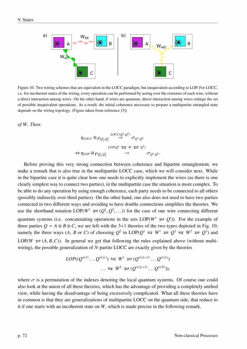
V. States

A B

C

WAC

WABa)

A B

C

WABC

b)

Figure 10. Two wiring schemes that are equivalent in the LOCC paradigm, but inequivalent according to LOP. For LOCC,i.e. for incoherent states of the wiring, every operation can be performed by acting over the extremes of each wire, withouta direct interaction among wires. On the other hand, if wires are quantum, direct interaction among wires enlarge the setof possible inequivalent operations. As a result, the initial coherence necessary to prepare a multipartite entangled statedepends on the wiring topology. (Figure taken from reference [5])

of W. Then:

ηLOCC ⊗ ρQ12,Q

22

LOCC(Q1,Q2)→ σQ1,Q2

⇔ ηLOP ⊗ ρQ12,Q

22

LOP(Q1 f→ W ← Q2)

→ σQ1,Q2 .

Before proving this very strong connection between coherence and bipartite entanglement, wemake a remark that is also true in the multipartite LOCC case, which we will consider next. Whilein the bipartite case it is quite clear how one needs to explicitly implement the wires (as there is oneclearly simplest way to connect two parties), in the multipartite case the situation is more complex. Tobe able to do any operation by using enough coherence, each party needs to be connected to all others(possibly indirectly over third parties). On the other hand, one also does not need to have two partiesconnected in two different ways and avoiding to have double connections simplifies the theories. Weuse the shorthand notation LOP(W1 ← (Q1,Q2, . . .)) for the case of one wire connecting different

quantum systems (i.e. concatenating operations in the sets LOP(W1 ← Qi)). For the example ofthree parties Q = A ⊗ B ⊗ C, we are left with the 3+1 theories of the two types depicted in Fig. 10;namely the three ways (A, B or C) of choosing Q2 in LOP(Q1 f→ W1 ← Q2 f→ W2 ← Q3) and

LOP(W ← (A, B,C)). In general we get that following the rules explained above (without multi-wiring), the possible generalization of N-partite LOCC are exactly given by the theories

LOP((Qσ(1) . . .Qσ( f1)) f→ W1 ← (Qσ( f1+1) . . .Qσ( f2))

. . . f→ WL ← (Qσ( fL+1) . . .Qσ(N))),

where σ is a permutation of the indexes denoting the local quantum systems. Of course one couldalso look at the union of all these theories, which has the advantage of providing a completely unifiedview, while having the disadvantage of being excessively complicated. What all these theories havein common is that they are generalizations of multipartite LOCC on the quantum side, that reduce toit if one starts with an incoherent state on W, which is made precise in the following remark.



Remark V.1. ∀ρW =∑

i pi|i〉〈i|W ,

1. TrW(Λ ◦ (ρW ⊗ 1Q)) ∈ LOCC(Q1, . . . ,Qn)

∀Λ ∈ LOP(Qi(1) f→ W j(1) ← Qi(2) f→ W j(2) ← . . .),

2. Λ ⊗ 1W ∈ LOP(Qi(1) f→ W j(1) ← Qi(2) f→ W j(2) ← . . .)

∀Λ ∈ LOCC(Q1, . . . ,Qn),

with i and j denoting permutations on the index sets. �

In the bipartite case, this means that if the initial state of the wire is incoherent and the wire isin a product states with both parties, tracing out the wire at the end reduces the theory to LOCC.The reason is that the state of the wire can be copied and stored in a local register on both sides.Every operation above can then just be obtained by local operations and broadcasting of classicalinformation, by updating the two local registers (just do the same permutations and phases on bothregisters, copy the information of measurements to both registers and trace out the corresponding partof a register on Bob’s side if Alice’s has been used in a quantum operation). We make this seeminglyobvious statement precise, because intuition sometimes might be misleading; for instance it is possibleto produce entanglement by sending a quantum particle back and forth that is never entangled witheither of the two parties [99]. While in entanglement theory this is surprising, since it means that onecan entangle two parties without using entanglement to do so, with the present approach the samestatement is very intuitive, as entanglement is simply not the only resource present, coherence andbasis dependent discord are resources as well. In the present approach without having resources onecannot entangle two parties, while any amount of basis-dependent discord allows to do that. This isbecause, as noted above, one can distillate coherence from any resource and the statement then justfollows from Thm. V.13, which we now prove.

Proof of Thm V.13. The “ ⇒ ” statement is a direct corollary of Rem. V.1 and Lem. V.1 on page 39.The operation B in Lem. V.1 allows to transform the state

∑i j ri, j|i〉〈 j|W ⊗ ρQ1

2,Q22

to∑

i j ri, j|ii〉〈 j j|W,Q22⊗

ρQ12,Q

22, which by classical to quantum forwarding can in turn be transformed to

∑i j ri, j|ii〉〈 j j|Q1

2,Q22⊗

ρQ11,Q

21

(by LOP(Q1 f→ W ← Q2) operations). By the Rem. V.1 we then get that the LOCC(Q1,Q2)

operation that reproduces Λ is also a LOP(Q1 f→ W ← Q2) operation, which concludes the proof ofthis direction.

For the converse, assume that a protocol is given, implementing Λ by elemental operations ofLOP(Q1 f→ W ← Q2), using an ancillary state

∑i j ri, j|i〉〈 j|W . To get the equivalent LOCC(Q1,Q2)

protocol using the ancillary state∑

i j ri, j|ii〉〈 j j|Q12,Q

22, replace the elemental operations of the given pro-

tocol in the following way by LOCC(Q1,Q2) operations:

1. Permutations:∑

i |σ(i)〉〈i|W , by permutations on both sides:∑

i |σ(i)〉〈i|Q12

followed by∑

i |σ(i)〉〈i|Q22.

2. Phases:∑

j ei φ( j)| j〉〈 j|W , by phases on one side:∑

j ei φ( j)| j〉〈 j|Q12

3. Observed quantum operations: |α〉Wa ⊗ KαQs , by the same operation, with the outcome in an

ancilla of the system Qs, classically communicating the result α to the other side Q¬s andencoding it there as well: |α〉Qs

a ⊗ KαQs followed by |α〉Q¬s

a .

PhD Thesis p. 73

V. States

4. Classical to quantum forwarding:∑

k〈k|Wa ⊗ |k〉Qsa , by first deleting the copy on Q¬s

2 (by doing aFourier measurement, followed by a correction of the phase on Qs

2, as in the proof of Lem. V.1),followed by the trivial forwarding:

∑k〈k|Qs

2⊗ |k〉Qs

a .

Note that by doing these replacements (and merging the ancillary Hilbert spaces with Q j2, j = 1, 2

after each step) a generic state∑

i, j si, j|i〉〈 j|W ⊗ τ(i, j)Q11,Q

21

in any step of the protocol gets mapped to∑i, j si, j|ii〉〈 j j|Q1

2,Q22⊗ τ(i, j)Q1

1,Q21, from which the assertion follows. �

In the following we are going to make a first step in the direction of using the theory of LOP toanalyse different types of multi-partite entanglement (see e.g. [101–105]). The analysis is facilitatedsince the above remark makes it easy to prove that the coherence needed to create entanglement givesa bound on the possible entanglement conversions, namely:

Theorem V.14. Let ρ, σ be states on W. If ∃τW , a state on W, s.t.

τW

LOP(Qi(1) f→ W j(1)...)

→ ρ,

but τW

LOP(Qi(1) f→ W j(1)...)

9 σ,

then it follows that ρLOCC(Q1,...,Qn)9 σ.

Proof. Assume the theorem is not valid, that is,

τW

LOP(Qi(1) f→ W j(1)...)

→ ρ,

τW

LOP(Qi(1) f→ W j(1)...)

9 σ

and

ρLOCC(Q1,...,Qn)→ σ.

From Rem. V.1 (point 2.) it follows that

ρLOP(Qi(1) f→ W j(1)...)

→ σ

and therefore

τW

LOP(Qi(1) f→ W j(1)...)

→ σ,

a contradiction. �



Note that for any of these theories (independently of the wiring) the free states are given by:

CQ(n)Z⊗

= {ρ | ρ =∑

m

pm|m〉〈m| ⊗ ρm, |m〉 ∈ Z⊗, ρm ∈ S EP(n)},

with Z⊗ the product basis of the incoherent basis of each wire, and S EP(n) the set of n−partiteseparable states

S EP(n) = {ρ | ρ =∑

k

pkρ(k)1 ⊗ . . . ⊗ ρ

(k)n }

This implies that for any of these theories,

RZ⊗,n(ρ) = minσ∈CQ(n)

Z⊗

S (ρ‖σ), (49)

with S (ρ‖σ) := Tr(ρ(log(ρ) − log(σ))) the relative entropy, defines an additive geometric monotone(see section V C). In general, the evaluation of this quantity is an NP-Complete problem [145]. How-ever, due to the monotonicity of the relative entropy, we notice that

RZ⊗,n(ρ) ≥ max(RZ⊗(TrQρ),REn (TrWρ)) (50)

being RZ⊗(TrQρ) the relative entropy of coherence on the wires, and REn (TrWρ) the relative entropy ofentanglement [58, 146, 147]. Due to the additivity of the relative entropy, if either RZ⊗(TrQρ) = 0or REn (TrWρ) = 0, Eq. (50) turns into an equality, providing a lower bound to the amount of initialcoherence required to prepare an entangled state among the parties of Q [47, 74].

As an example of how this perspective can be applied in the multipartite case, let us revisit the caseof the |W〉 and of the |GHZ〉 state [100]. To this end, we start by looking at how much coherence onthe wire we need to generate the respective states.

Example V.1. The least coherent state necessary to produce the state |GHZn〉Q1,...,Qn = 1√

2(|0〉⊗n+|1〉⊗n)

using LOP(W ← Q1 ⊗ . . .Qn) is given by

|+〉W =1√

2(|0〉W + |1〉W).

Similarly, one can produce the state |Wn〉Q1,...,Qn = 1√

n (|0, . . . 0, 1〉 + . . . |1, 0, . . . , 0〉

using LOP(W ← Q1 ⊗ . . .Qn) from

|+log2(n)〉W =1√

n(|0〉 + . . . + |n − 1〉).

The least coherent state necessary to produce the state |GHZn〉Q1,...,Qn

using LOP(Q1 f→ W1 ← Q2 f→ . . .Wn−1 ← Qn) is given by

|+n−1〉W1,...Wn−1 = (1√

2(|0〉 + |1〉))⊗(n−1).

Similarly, one can produce |W3〉Q1,Q2,Q3 ,

using LOP(Q1 f→ W1 ← Q2 f→ W2 ← Q3) from

|+W〉W1,W2 :=1√

2(|0〉 + |1〉) ⊗

1√

3(|0〉 +

√2|1〉).

PhD Thesis p. 75

V. States

Proof. We start by giving explicit protocols that do the conversions. For the |GHZn〉Q1,...,Qn state, wesimply apply a CNOT (a permutation) on |+〉W1 ⊗ |0〉

(n−1)W2,...,Wn−1

n − 1 times (on W1,W j), resulting in|GHZn〉W , then forward the respective subsystems.

For the |Wn〉Q1,...,Qn state we apply a permutation that acts as

|i〉W1 ⊗ |0〉(n−1)W2,...,Wn−1

7→ |0〉W1 . . . |0〉|1〉Wi |0〉 . . . |0〉Wn−1

to

|+log2(n)〉W1 ⊗ |0〉(n−1)W2,...,Wn−1

=1√

n(|0〉 + . . . + |n − 1〉) ⊗ |0〉(n−1)

W2,...,Wn−1

and forward the subsystems to the different parties. That the generation of the |GHZn〉 state is optimalis simply seen by the fact that |GHZ2〉 is the state with the minimal coherence rank [115] havingthe relative entropy of coherence [8] equal to the relative entropy of entanglement [58, 146, 147] of|GHZn〉Q1,...,Qn , namely 1.

For the case with more than one wire, to prepare the |GHZn〉Q1,...,Qn state from |+n−1〉W1,...,Wn−1 , we doa local CNOT on each wire, after preparing an ancillary state |0〉W j

2, effectively "doubling" the states,

resulting in |GHZ2〉⊗(n−1)(W1

1 ,W12 ),...,(Wn−1

1 ,Wn−12 )

. We then forward each half of the system of the respective

wires to the quantum systems they connect, resulting in |GHZ2〉⊗(n−1)(Q1

1,Q21),(Q2

2,Q31),...,Qn−1

1 ,(Qn−12 ,Qn

1). We can

then double the system Q21, resulting in the state |GHZ3〉Q1

1,Q21,Q

23. We can then use the |GHZ2〉(Q2

2,Q31)

to teleport the system Q23 to Q3

3, and so on. Iteratively we get the wanted |GHZn〉Q1,...,Qn state. Theoptimality follows from any bipartitions being equivalent to |GHZ2〉 states.

Starting from the |+W〉W1,W2 state, we first "double" each of the sides, then make a permutation1 ↔ 0 on the site W2

2 which puts the system into the state: |GHZ2〉W11 ,W

12⊗√

2√

3(|0, 1〉 + 1

√3|1, 0〉)W2

1 ,W22.

We continue by forwarding the system W22 to Q2

1. On this site (Q2) we then continue by applyingthe operation |0, 0〉Q2

1,Q22〈0|Q2

1+ 1√

2|0, 1〉Q2

1,Q22〈1|Q2

1+ 1√

2|1, 0〉Q2

1,Q22〈1|Q2

1leaving us with the |W〉 state

on Q21 ⊗ Q2

2 ⊗ W21 . The next step is to forward the system W2

1 to Q3. Finally one can distribute the|GHZ2〉W1

1 ,W12

state to the connected quantum systems (yielding |GHZ2〉Q11,Q

23), and use this to teleport

via LOCC and hence LOP the system Q22 to Q1

2. The protocol hence results in |W〉Q12,Q

21,Q

3 . �

We can use this example to provide an alternative proof that the two classes |GHZ〉 and |W〉 areinequivalent. The relative entropy of entanglement of |GHZn〉 = |0〉⊗n−|1〉⊗n

√2

is 1 [146] and indeed one can

prepare the |GHZn〉 state by LOP(W ← (Q1,Q2, . . . ,Qn)) from |0〉+|1〉√

2. For |Wn〉 =

∑n−1k=0 |0〉

⊗k |1〉|0〉⊗n−k−1√

nthe relative entropy of entanglement is (n − 1) log2(n/(n − 1)) > 1∀n > 2 [147]. It is then a simple

corollary of Thm. V.14 that |GHZn〉LOCC(Q2,...,Qn)9 |Wn〉.

The second thing to note is that on any bipartition the |GHZn〉 state is LOCC equivalent to |GHZ2〉,while the |W3〉 state on any bipartition is LOCC equivalent to 1/

√3(|00〉 +

√2|11〉). Indeed one can

in all three possible two-wire settings LOP(Q1 f→ W1 ← Q2 f→ W2 ← Q3) prepare |W3〉 from

1/√

6(|0〉+√

2|1〉)W1⊗(|0〉+|1〉)W2 , while the bipartite entanglement one can produce on the bipartitionQ1, (Q2 ⊗ Q3) is not enough to prepare |GHZ3〉: as on any bipartition one needs to prepare a fullyentangled qubit and this is equivalent to a maximally coherent qubit, the state with minimal coherenceto prepare |GHZ3〉 is given by 1/2(|0〉 + |1〉)W1 ⊗ (|0〉 + |1〉)W2 , which is strictly more coherent on



W1 than 1/√

6(|0〉 +√

2|1〉)W1 ⊗ (|0〉 + |1〉)W2 . Again as a corollary of Thm. V.14, we have that

|W3〉LOCC(Q1,Q2,Q3)9 |GHZ3〉.

In total this gives a strong indication that the resources in the different types of wirings correspondto different types of entanglement. How this connection is generalises to more complicated settings(for instance four parties or three parties with qutrits instead of qubits) is an interesting (and non-trivial) question, we have to leave open for future work.

We finish this chapter by giving a (not exhaustive) overview on the zoo of different resource theo-ries of coherence, basis-dependent discord and entanglement.

H. Relation to different classes of operations

In this section we give additional details on the relation between LOP and some selected classes ofoperations discussed in the literature, see Fig. 11. A complete representation is beyond the scope ofthis thesis, but the interested reader can find more references to relevant articles about these and otherclasses in [46]. For coherence theory, the biggest classes of operations we want to mention are two

Figure 11. Venn-diagram for the inclusion relations of LOP with selected coherence theories (left), theories of basis-dependent discord (middle) and entanglement theories (right), within general CPTP operations (see [46] for additionalclasses). (Figure adapted from reference [5]).

natural classes whose action on the set of incoherent states can be modelled by stochastic operationsand are closed under composition and mixing [7]. These are the ones that do not create coherence onaverage (the maximally incoherent operations MIO [60]) and those that cannotz influence populationby the presence of coherence (coherence non-activating operations CNA [75, 76]). The intersectionof these two sets are the operations that can neither create nor detect coherence – the dephasingcovariant operations (DIO [75, 77, 78]). They are called so because they commute with dephasing.MIO contains a subset of operations that do not generate coherence even after post-selection, theincoherent operations (IO [8]). LOP(W ← 1) (meaning the effective coherence theory of LOP on thewire) is similar to IO, but not equivalent. LOP has a more complicated structure, but is operationallymotivated in this thesis. Subsets of LOP are the strictly incoherent operations (SIO [45, 79]), which

PhD Thesis p. 77

V. States

include the physical incoherent operations (PIO [77]) that in turn have the translationally invariantoperations (TIO [61, 78]) as a sub-set. Note that for the inclusion of TIO in PIO and SIO to be valid,the Hamiltonian of the system needs to be non-degenerate or, conversely, one needs to generalizecoherence theory to a theory where the dephasing defining incoherent states is not total and leavesthe degenerate subspaces of the Hamiltonian invariant (see [60, 78]). These three theories (SIO, TIOand PIO) also have operationally sensible interpretations (for instance TIO play an important rolein thermodynamics [148, 149]). However, since SIO, TIO and PIO are subsets of DIO, they cannotcreate nor detect coherence (restricting the free POVMs to a very small set, namely all those thatcannot measure coherence). This means that coherence is not a useful resource for any task that isobservable by free measurements in these sets.

Not depicted in Fig. 11 are the theories of unspeakable coherence [78]. Unspeakable informationis information that can only be encoded in certain degrees of freedom, a definition which stems fromthe resource theory of frames [150]. Such a restriction can certainly be relevant in many physicalsettings when it marks a practical border between easily and not easily implementable operations forthem (e.g. in quantum metrology, reference frame alignment and quantum thermodynamics; see [78]for a discussion and references). However it has nothing to do with a conceptual frontier betweenclassical and quantum physics (however operational the description). Since this thesis is about thelatter distinction, we only describe theories of speakable coherence.

For basis-dependent discord, we first have the class that leaves incoherent-quantum states invariant,even after post-selection, the incoherent-quantum operations (IQO [74]). Inside these (though it isstill an open question whether this inclusion is strict), we have the general operations incoherent onA (GOIA [3], here A = W). These operations are very similar, but not equivalent, to LOP(W ← Q).Instead of allowing permutations on the wire, in GOIA any incoherent operations is allowed, makingGOIA slightly less operationally meaningful. SIO [79], TIO [78] and PIO [77] can also be formulatedas effective theories of basis-dependent discord theories, which, for convenience, we still call SIO,TIO and PIO. The connection between these extended versions of SIO, PIO and LOP(W ← Q) isgiven in the discussion of Prop. V.4. We also depict the set of local quantum incoherent operations andclassical communication LQICC in this connection [90]. This set lies within GOIA by construction.Since it does not include forwarding of states, as the interaction between the two parties is limited toclassical communication (or classical control), so it does not include LOP nor SIO and thus is a strictsubset of GOIA, where with classical control we mean local operations conditional to measurementoutcomes (a special case of quantum control defined in Eq. 30). LQICC includes all incoherentoperations on one side, which are not included in LOP and one can easily see that PIO lies inside.This set is also interesting as it has been used to analyse steering induced coherence (see e.g. [92, 93]).

For entanglement between two distant parties one has the set of separable operations (SEP [58])that preserve separable states (states with no entanglement). Inside of these there are the better op-erationally motivated, but more complex, local operations and classical communication (LOCC [58,151]). This set is the same as the effective theory of LOP on the two parties, LOP(Q1 f→ 1 ← Q2).Replacing the permutations on the wire in the basic definition of LOP by the identity or by incoherentoperations we still get the same effective theory, LOCC. However, in the proof of Thm. V.13 (concern-ing the equivalence of the resources coherence and entanglement in the bipartite setting) we do needthe permutations for one direction and for the other we do use that LOP only consists of the elemental


H. Relation to different classes of operations

operations presented here. Therefore it is not clear for other sets of incoherent operations, whethercoherence on the wire and entanglement between the two parties are equivalent resources for bipartitetasks. Inside LOCC finally, there are the operations that additionally to the locality restriction alsoask that the local operations of one party is incoherent in a given basis (LQICC). Asking that boththe parties are incoherent in a given basis, one finally gets the local incoherent operations and clas-sical communication (LICC [48, 91]). Replacing the incoherent operations there by LOP(W ← 1),

we get LOP(W1 ← 1 f→ 1 ← 1 f→ W2) (meaning that the local environment of the two parties isconnected by a wire).

In conclusion we note that LOP, both for (speakable) coherence as also for basis-dependent dis-cord, is the only set of operations we know so far that can be characterized by a simple set of op-erationally meaningful operations, while at the same time can make use of coherence as a resource.In fact, in any theory with free operations being a subset of DIO (that is DIO, SIO, PIO and TIO),coherence can never be detected, so, even though coherence does allow to do operations that other-wise are not possible, the action of these can never be seen by projective measurements on the set offree states. On the other hand any theory that includes incoherent operations currently lacks a fullyoperational description; because up to now, we do not know a minimal generating set of operationsfor this set, that has a transparent operational meaning. LOP is the set that comes closest to achievingthis so far.

PhD Thesis p. 79

VI. COHERENT MAPS


We argued in section V B on page 44, that it is not possible to build a meaningful resourcetheory if one cannot detect resources for free. On the other hand we saw that measuringcoherence is a crucial task for quantum advantage, as important as creating it. How then canone quantify the ability to detect coherence? We answer this question in the current chapter,where we look at coherence as a resource on the level of maps.

This chapter follows closely, mostly literally, the preprint of Ref. [6]. In the last section we anal-ysed which states can be considered classical under different circumstances, and also introduced themeans to quantitatively compare the non-classicality of the states. As special cases we could recoverand give additional meaning to the entangled states, discord states classical-quantum states and co-herent states. We also showed that if enough resources are present one can use them to fuel whateveroperations. Therefore it makes sense to approach the complementary question to ask how valuablethese operations are [152] by the evaluation of quantities such as the resource generation capacity,i.e. the maximal increase of the resource in an input state under application of the operation, or theresource cost, that is, the minimal amount of resources needed to simulate a non-free operation bymeans of free operations [2, 153–159]. One could imagine that nothing else is needed to characterizethe non-classicality of processes. However this is not true. Classicality depends a lot on the context.While to prepare arbitrary states can be a major problem in experiments, often it is also not easy tomeasure them in arbitrary directions. More conceptually, most schemes for quantum computationpresume that one prepares the state in the computational basis, but also that the read-out is in thesame basis. As we have seen in chapter IV, if we just consider one given Markovian dynamics, non-classical processes are those that both create and detect coherences. One could be tempted to try toquantify the ability to detect non-classicality, by asking how much resources (in states) one needs tomake an operation that allows to do this. But there is no way to make sense of such an approach. Wecan see this by noting that there are two types of resource theories of states. In the first type there aresome operations that are free and allow you to detect what resource state you have. Then detectionof coherence is free by definition, and no resources are needed for this task. In coherence that is forinstance the case for LOP, described in the last section [5], as well as for IO [8] and MIO [60]. Onthe other hand one can ask that no operations are allowed that show how much resources are presentin a state, but then, how do you know that you have a resource state in the first place? And evenmore problematic in this context, if you do have a resource state, there will be no free operation thatallows you to reveal anything about the amount of resource present, meaning that there is no state thatallows you to detect resources. This is for instance the case for all the resource theories of coherencecontained in CNA (see Fig.11 on page 77). We are left in the paradoxical situation that either theresource theory does not makes sense of the notion that states can be a resource, or it does not makesense of the notion that detecting resource states is a resource. In both cases we cannot measure theability to detect coherence through the amount of resource present in a state. Of course one could tryto make a hybrid approach, but what would be the operational motivation for that?

Here we proceed differently. The property that we want to analyse is the ability to detect coherence.

p. 80

A. Measuring the coherence detecting ability of maps

So we build a resource theory for this dynamic property. We will see that this resource theory easilyfits into our framework for theories of non-classicality, making a clear-cut connection between non-classical maps and classical ones within this theory. More concretely, we will build formal resourcetheories on the level of operations, allowing to quantify the value of operations directly. This is alsointeresting from a conceptual point of view as the goal of quantum technologies is to perform sometasks that are impossible using classical technologies. This includes sensing at high precision [160],efficient processing of information, and secure transmission of data [120]. Ultimately, this is alldone by quantum operations, i.e. dynamical resources. Therefore it seems natural to quantify thevalue of operations directly without the detour through states, which are static resources that have tobe transformed into dynamic resources using free operations. Since quantum states can be seen asquantum operations with no input and a constant output, a resource theory on the level of operationscan quantify the value of states too, leading to a unified resource theoretic treatment of states andoperations. Therefore we expect that resource theories on the level of operations will be a key methodto the systematic exploration of quantum advantages.

In detail, we will show that the coherence detection capability of operations can be quantifiedrigorously and that the conceptual problem discussed above vanishes if we use a resource theory onthe level of operations. We will first introduce the two basic ingredients to such a theory: The freeoperations and the free super-operations, which correspond naturally to sequential and parallel con-catenations with free operations [56, 161, 162]. From these ingredients we deduce defining propertiesof functionals which are well suited to quantify the value of operations. Then we present two suchfunctionals quantifying how well an operation can detect coherence, one based on the diamond normthat can be calculated efficiently and the other one with a clear operational interpretation which isbased on the induced trace norm. We give examples for the value of operations according to thesemeasures and conclude with an outlook on open questions. The framework we introduce can be easilyextended to operations that cannot create coherence and operations that can neither detect nor createit.


We want to quantify how well a quantum operation can detect coherence. As explained in theintroduction, we aim at building a resource theory on operations for this task, which requires thatwe define the free operations and super-operations. As the statistics of any measurement in quantummechanics can be described by a Positive Operator-Valued Measure (POVM), we start by observingwhich of these do not detect coherence. This is the case, if the measurement statistics of the POVMis independent of the coherence in the state it measures (such that measuring a state ρ yields the sameprobabilities as measuring its dephased state ∆ρ), which leads us to the following definition:

Definition VI.1. A POVM given by {Pn} : Pn ≥ 0,∑

n Pn = 1 is free iff

Tr Pn∆ρ = Tr Pnρ ∀ρ, n. (51)

As one expects, all free POVMs are diagonal in the incoherent basis (see the proof in Sec. VI A 1):

PhD Thesis p. 81

VI. Maps

Proposition VI.1. A POVM is free iff

Pn =∑

i

Pni |i〉〈i| ∀n. (52)

In other words, the free measurements are the convex combination of the measurements we use todefine coherence theory, the orthogonal projective measurements defining the incoherent basis.

Next we define general free operations, where we need to address subselection (by measurementresults) in a consistent manner. Since the ability to do subselection depends on the actual experimentalimplementation, we adopt the point of view that this is a resource in itself. In general, we can havea quantum instrument (mx,Mx)x =

(Tr[Ex·], (Ex(·)/Tr[Ex·])x

)which allows us to do subselection

according to a variable x, i.e we obtain with probability px = mx(ρ) = TrEx(ρ) an output ρx =

Mx(ρ) = Ex(ρ)/px. From the definition of the free POVMs follows that we can store the outcome x inthe incoherent basis of an ancillary system, which we write as

M(ρ) =∑

x

Mx(ρ) ⊗ |x〉〈x|, (53)

and implement the subselection later using the orthogonal measurement in the incoherent basis on thesecond subsystem. In the special case of a POVM P, we can represent it by

P(ρ) =∑

n

Tr(Pnρ)|n〉〈n|. (54)

Treating subselection in this way, we can reduce our analysis to trace preserving operations.As we focus on the detection of coherence, we do not care about how much coherence an operation

can produce, and hence any preparation should be free, meaning that all states are free. We wantto look at the maximal set of operations that is classical with this restriction. We call a quantumoperation free if it cannot turn a free POVM into a non-free one by applying the operation prior to themeasurement. This is exactly the case if it cannot transform coherences into populations [75].

Definition VI.2. A quantum operation Φ is called detection-incoherent iff

∆Φ =∆Φ∆. (55)

The set of detection-incoherent operations is denoted by CNA (for coherence non-activating), forsimplicity (instead of F CNA

O).

Note that this condition has been called nonactivating in [76]. With our convention for treatingsubselection, this includes Def. VI.1 for POVMs. As we mentioned in the introduction, it is bothimportant to create and to detect coherence, therefore one can define creation-incoherent operations,i.e. operations which cannot create coherence. In coherence theory, these operations are called MIO(for maximally incoherent operations) [60, 163] or nongenerating in a general context in [76], or CIfor creation-incoherent [6]. Operations that can neither create nor detect coherence are called DIO(dephasing-covariant incoherent operations) [77, 78, 164, 165], classical operations [75] or commut-ing [76], orDCI for detection-and-creation-incoherent [6].



Definition VI.3. A quantum operation Φ from system A to B is called creation-incoherent, if it cannotcreate coherence in system B if none was present in system A,

Φ∆ =∆Φ∆. (56)

It is called detection-creation-incoherent if it can neither detect nor create coherence,

∆Φ = Φ∆. (57)

Our contribution in the work [6], on the preprint of which this chapter is based, was to show howto quantify the abilities to create and detect coherence in a rigorous manner. Note that the threedefinitions of free operations lead to different resource theories. In general, we can check directly ifa quantum operation is free: Every quantum operation Φ is linear and thus completely determined bythe coefficients Φk,l

i, j (see Appendix A on pages 122 to 128) defined through

Φ (|k〉〈l|) =∑

i, j

Φk,li, j |i〉〈 j|. (58)

For the definitions above, it is straightforward to check that the coefficients need to be given as in thefollowing proposition (see the proof in section VI A 1).

Proposition VI.2. Let us represent a linear map Φ(ρ) by the coefficients Φb,da,c as above. Then Φ is

completely positive iff

Φb,da,c =

∑n

Kna,b K∗nc,d. (59)

Under this condition,Φ is a detection-incoherent quantum operation iff

Φb,da,a = p (a|b) δb,d∀a, b, d. (60)

Φ is a creation-incoherent quantum operation iff

Φa,ab,c = p (b|a) δb,c ∧

∑a

Φb,da,a = δb,d.∀a, b, d. (61)

Φ is a detection-creation-incoherent operation iff

Φb,da,a = p (a|b) δb,d∀a, b, d,

Φa,ab,c = p (b|a) δb,c∀a, b, d. (62)

In the following, we will use “free operation” if it is unimportant which specific choice we areconsidering. This allows us to introduce the second ingredient to our resource theories, the freesuper-operations, in a unified manner. A super-operation is free if it is a sequential and/or parallelconcatenation with free operations.

PhD Thesis p. 83

VI. Maps

Definition VI.4. For free operations Φ, elemental free super-operations are given by

E1,Φ [Θ] =Φ ◦ Θ, E2,Φ [Θ] = Θ ◦ Φ,

E3,Φ [Θ] =Θ ⊗ Φ, E4,Φ [Θ] = Φ ⊗ Θ. (63)

A super-operation F is free iff it can be written as a sequence of free elemental super-operations,

F = Ein,Φn ...Ei3,Φ3Ei2,Φ2Ei1,Φ1 . (64)

This definition comes from a quantum computational setting: a free super-operation is an embed-ding into a free network (see e.g. [55]). A minimal requirement on the free super-operations is thatthey transform free operations into free operations, otherwise it would be possible to create resourcesfor free. Explicitly (the proof is trivial, for completeness we also give it in section VI A 1):

Lemma VI.3. If both Φ and Θ are free, Φ ◦ Θ and Φ ⊗ Θ are free as well.

One might worry, that Def. VI.4 introduces a highly non-trivial family of super-operators, as it isbased on elemental super-operators and in principle such a construction is not guaranteed to allow fora finite representation. This is for instance the case in entanglement theory, where it has been shownthat there is no finite representation in general. Remarkably however, in this case it is straightforwardto show that every free super-operation can be composed using only three elemental operations. Theproof is based on ideas from [56, 161] and can be found in section VI A 1.

Proposition VI.4. A super-operation F is free if and only if it can be written as

F [Θ] = FΦ2,Φ1 [Θ] :=Φ2 ◦ (Θ ⊗ 1) ◦ Φ1 (65)

where Φ1 and Φ2 are free.

While we focus on the ability to detect coherence in this section, we present a few results forthe other two classes of free operations inside NCGD (namely MIO and DIO) (see also [75, 163]).The case of coherence treated here is an example of our general set-up: If one exchanges the re-source destroying map ∆ (by some other map that destroys a different resource than coherence) inthe Defs. VI.2, VI.3, and VI.4, one gets other resource theories. It is also possible to define freeoperations without the usage of resource destroying maps and to use directly Def. VI.4 for free super-operations [161].

1. Proofs

Here we present the proofs of Prop. VI.1, Lem. VI.3 and Prop. VI.4 above. We start with the formof the free POVMs in the detection-incoherent setting.

Proposition (VI.1). A POVM is free iff

Pn =∑

i

Pni |i〉〈i| ∀n. (66)



Proof. Let us use the notation

Pn =∑

i, j

Pni, j|i〉〈 j| (67)

and

|ψ〉 =1√

2

(|a〉 + eiφ|b〉

)(68)

with a , b and φ ∈ R. Now assume that the POVM is free. From Def. 1 in the main text, it follows,for ρ = |ψ〉〈ψ|,

Tr Pn∆ρ = Tr Pnρ

⇔ Pna,a + Pn

b,b = Pna,a + Pn

b,b + Pna,be−iφ + Pn

b,aeiφ

⇔ 0 = 2 Re(Pn

a,be−iφ)

(69)

such that

Pn =∑

i

Pni |i〉〈i| ∀n (70)

is a necessary condition. It is obviously also sufficient. �

Lem. VI.3 says that the free operations are closed under free super-operations, which is basicallyclear by definition.

Lemma (VI.3). If both Φ and Θ are free, Φ ◦ Θ and Φ ⊗ Θ are free as well.

Proof.

ΦMIOΘMIO∆ = ΦMIO∆ΘMIO∆ = ∆ΦMIO∆ΘMIO∆ = ∆ΦMIOΘMIO∆,

∆ΦCNAΘCNA = ∆ΦCNA∆ΘCNA = ∆ΦCNA∆ΘCNA∆ = ∆ΦCNAΘCNA∆,

(ΦMIO ⊗ ΘMIO) ∆ = (ΦMIO∆) ⊗ (ΘMIO∆) = (∆ΦMIO∆) ⊗ (∆ΘMIO∆) = ∆ (ΦMIO ⊗ ΘMIO) ∆,

∆ (ΦCNA ⊗ ΘCNA) = (∆ΦCNA) ⊗ (∆ΘCNA) = (∆ΦCNA∆) ⊗ (∆ΘCNA∆) = ∆ (ΦCNA ⊗ ΘCNA) ∆. (71)

�

This shows that our free super-operations indeed preserve the set of free operations. In addition, itallows us to give the following simplified characterization of the free super-operations (see also [56]and lemma 3.11 in [161]).

Proposition (VI.4). A super-operation F is free if and only if it can be written as

F [Θ] = FΦ2,Φ1 [Θ] :=Φ2 ◦ (Θ ⊗ 1) ◦ Φ1 (72)

where Φ1 and Φ2 are free.

PhD Thesis p. 85

VI. Maps

Proof. First we note that

FΦ2,Φ1 [Θ] = E1,Φ2 ◦ E2,Φ1 ◦ E3,1 [Θ] (73)

is always free by definition. Defining the (in all three frameworks) free operation

ΦS (ρ ⊗ σ) = σ ⊗ ρ, (74)

we can write all elemental free operations in this form,

E1,Φ [Θ] =Φ ◦ Θ = Φ ◦ (Θ ⊗ 1) ◦ 1 = FΦ,1 [Θ] ,

E2,Φ [Θ] =Θ ◦ Φ = 1 ◦ (Θ ⊗ 1) ◦ Φ = F1,Φ [Θ] ,

E3,Φ [Θ] =Θ ⊗ Φ = (Θ ⊗ 1) ◦ (1 ⊗ Φ) = 1 ◦ (Θ ⊗ 1) ◦ (1 ⊗ Φ) = F1,1⊗Φ [Θ] ,

E4,Φ [Θ] =Φ ⊗ Θ = ΦS ◦ (Θ ⊗ Φ) ◦ ΦS = ΦS ◦ (Θ ⊗ 1) ◦ (1 ⊗ Φ) ◦ ΦS = FΦS ,(1⊗Φ)◦ΦS [Θ] . (75)

Therefore

FΦ4,Φ3 ◦ FΦ2,Φ1 [Θ] =Φ4 ◦ [(Φ2 ◦ (Θ ⊗ 1) ◦ Φ1) ⊗ 1] ◦ Φ3

=Φ4 ◦ [(Φ2 ⊗ 1) ◦ (((Θ ⊗ 1) ◦ Φ1) ⊗ 1)] ◦ Φ3

=Φ4 ◦ (Φ2 ⊗ 1) ◦ [((Θ ⊗ 1) ⊗ 1) ◦ (Φ1 ⊗ 1)] ◦ Φ3

=Φ4 ◦ (Φ2 ⊗ 1) ◦ [Θ ⊗ 1 ⊗ 1] ◦ (Φ1 ⊗ 1) ◦ Φ3

=Φ4 ◦ (Φ2 ⊗ 1) ◦ [Θ ⊗ 1] ◦ (Φ1 ⊗ 1) ◦ Φ3

=FΦ4◦(Φ2⊗1),(Φ1⊗1)◦Φ3 [Θ] (76)

finishes the proof. �

Proposition VI.5. VI.2 Let us represent a linear map Φ(ρ) by the coefficients Φb,da,c as above. Then Φ

is completely positive iff

Φb,da,c =

∑n


Under this condition,Φ is a detection-incoherent quantum operation iff

Φb,da,a = p (a|b) δb,d∀a, b, d. (78)

Φ is a creation-incoherent quantum operation iff

Φa,ab,c = p (b|a) δb,c ∧

∑a

Φb,da,a = δb,d.∀a, b, d. (79)

Φ is a detection-creation-incoherent operation iff

Φb,da,a = p (a|b) δb,d∀a, b, d,

Φa,ab,c = p (b|a) δb,c∀a, b, d. (80)



Proof. Φ being completely positive is equivalent to Φ (ρ) =∑

n KnρK†n which we can write as

Φ(ρ) =∑

n,i, j,a,b,c,d

Kna,b |a〉〈b|ρi, j|i〉〈 j|K∗nc,d|d〉〈c| =

∑n,a,b,c,d

Kna,b K∗nc,dρb,d|a〉〈c| (81)

from which follows

Φb,da,c =

∑n


Now we come to the first part of the proposition. We have

∆Φρ =∑a,b,d

Φb,da,aρb,d|a〉〈a|,

∆Φ∆ρ =∑a,b

Φb,ba,aρb,b|a〉〈a|. (83)

Thus Φ being detection-incoherent is equivalent to∑b,d

Φb,ds,sρb,d =

∑b

Φb,bs,sρb,b∀s, ρ, (84)

which is exactly the case if this condition holds for all pure ρ = |ψ〉〈ψ| with

|ψ〉 =∑

j

√q jeiγ j | j〉, (85)

meaning Φ is detection-incoherent iff∑b,d

Φb,ds,s√

qb√

qdei(γb−γd) = 0∀s, {qi}prob. distr., γi ∈ R. (86)

From this follows the necessary condition

0 =12

(Φb,d

s,s ei(γb−γd) + Φd,bs,s ei(γd−γb)

)=<

∑n

Kns,b K∗ns,dei(γb−γd)

∀s, b , d, γb ∈ R, γd ∈ R (87)

(88)

and thus ∑n

Kns,b K∗ns,d= Φb,d

s,s = 0∀s, b , d. (89)

In addition, since we work with trace preserving operations, we have

p(a|b) = 〈a|∑

n

Kn|b〉〈b|K†n |a〉 =∑

n

Kna,b K∗na,b= Φb,b

a,a (90)

and therefore necessarily ∑n

Kns,b K∗ns,d= Φb,d

s,s = p (a|b) δb,d∀a, b, d. (91)

PhD Thesis p. 87

VI. Maps

This is already sufficient for trace preservation, since

1 =∑

n

K†n Kn ⇔∑n,a

Kna,b K∗na,d=

∑a

Φb,da,a = δb,d. (92)

To show that condition (78) is also sufficient, we can plug it into condition (86)∑n,b,d

Kns,b K∗ns,d

√qb√

qdei(γb−γd) =∑b,d

p (s|b) δb,d√

qb√

qdei(γb−γd) = 0∀s, {qi}prob. distr., γi ∈ R, (93)

and see that it is satisfied.Now we come to the second part. Assume Φ is creation-incoherent. From

Φ (|i〉〈i|) =∑k,l

Φi,ik,l|k〉〈l| (94)

and the condition ∆Φ∆ = Φ∆, we find

Φi,ik,l = Φi,i

k,kδk,l∀i. (95)

Since Φ is a trace preserving quantum operation and |i〉〈i| a valid density operator, Φi,ik,k have to be a

non-negative real numbers with∑

k Φi,ik,k = 1. Thus p(k|i) = Φi,i

k,k defines conditional probabilities andwe end up with the condition

Φi,ik,l =p(k|i)δk,l∀i, k, l. (96)

This time, we need to enforce trace preservation separately, again by the condition∑a

Φb,da,a = δb,d. (97)

Sufficiency is straight forward, the third statement a trivial consequence of the others. �

B. Connection to the framework of non-classicality

We have seen that the the two main convex subsets of the NCGD operations discussed in chap-ter IV, namely the ones that do not detect coherence (CNA) and the ones that do not create coherence(MIO), provide the basis of meaningful resource theories on the level of operations. Not clarifiedyet is the connection to classicality. We will go back to the definitions in section II A to draw thislink, but first we need to recollect all the elements of the theories.For both theories we can take asfree measurements destructive ones in a fixed basis (FMCNA = FM

MIO = {{λi, 〈i|}i}~λ); for the case ofCNA, Prop. VI.1 says exactly this, in principle one could take measurements in any basis for the caseof MIO, but we can also do these by doing a free operation first which does the measurement andencodes the output in the incoherent basis and then measure that basis, a similar statement is validfor getting the measurement outcome of arbitrary free instruments in both cases. The free operationsare different however, CNA,MIO (see the definitions VI.2 and 19). For the first set any state prepa-ration is free, which means that any quantum state is a free state FSCNA = S, for the second set, bydefinition we care about not the ability to prepare coherence, which means that the free states should


B. Connection to the framework of non-classicality

be incoherent FSMIO = {∑

i pi|i〉〈i|}. We also introduced a set of super-operations which we call free,namely embedding an operation into a network of free operations VI.4. This can be simplified a lot(see Prop.VI.4). This can be understood in the framework we introduced by noting that, here, we re-strict our analysis to the most common framework of information theory, where one usually thinks interms of protocols consisting of parallel executions or concatenations of operations, with each beingunaffected by the ones done before (up to post-selection by measurements, but that can, without lossof generality, be postponed to the end of a protocol). We leave the question open, how one can tacklea more generic open quantum system setting, where the dynamics may be non-Markovian and hencedepend not only on how one operates on the system at a certain instance in time, but also on whatone did before and on the specific interactions of the system with the environment and its evolution.Accordingly, the free changes of the dynamics can be described by super-operations that correspondto such a protocol. While (as is usual in quantum information) we do not specify a time variable, thetimes at which one can measure T are restricted to be between the operations, and hence discrete.

Of course any free operation can be simulated classically, when applied on the set of free states.This is because by definition the free operations act equally on all the free states with the samepopulations and we can only measure it at the beginning and at the end. The statistics we get is henceone-time and classical. This means that we can associate to every operation a stochastic operationthat gives rise to the same statistics, that is, we have a mapping R : CPT P→ S toc, where S toc is theset of stochastic matrices, such that

m[Λ[ρ]] = (R[Λ])m[ρ], ∀ρ ∈ FS (98)

What we need to ask is when a full protocol is classical. Assuming that we have a protocol and domeasurements in between followed by preparing (using a free operation) a free state that correspondsto the outcome measured (that is a state σ, such that mi[σ] = 1, if one measured the outcome i of thefree measurement (m,M)), can the multi-time statistics be explained by a stochastic process?

In a way, this is what Lem. VI.3, about the closeness of the free operations under concatenationand parallel execution, guarantees. To elaborate a bit more, Eq. 98 yields for concatenation:

m[Λ2 ◦ Λ1[ρ]] = (R[Λ2])m[Λ1[ρ]]

=∑

i

((R[Λ2])ei)mi[Λ1[ρ]]

=∑

i

m[Λ2[Πi]]mi[Λ1[ρ]], ∀ρ ∈ FS, (99)

where we defined ei to be the unit real vector corresponding to the outcome i (m =∑

i miei), and Πi afree state that corresponds to the outcome i. We applied Eq. 98 in the first (where we also needed thatfree states are mapped to free states) and last equation and linearity in the second. As concatenationsof free operations are free (Lem. VI.3), the same argument extends to arbitrary concatenations. Theequations we get are just the Kolmogorov consistency conditions, Eq. 3. So there is a classicalstochastic process explaining the evolution. From the last section we should be a bit careful andask, whether there is also a classical stochastic process that respects local behaviour, meaning that if

PhD Thesis p. 89

VI. Maps

you do two operations in parallel, they really act on separate classical spaces. This is indeed the case:

m[Λ1 ⊗ Λ2[ρ]] = (R[Λ1 ⊗ Λ2])m[ρ]

=∑

i, j

((R[Λ1 ⊗ Λ2])ei ⊗ e j

)mi, j[ρ]

=∑

i, j

m[Λ1[Π1

i ] ⊗ Λ2[Π2j]]

mi, j[ρ]

=∑i, j,k,l

(ek ⊗ el)m1k

[Λ1[Π1

i ]]

m2l

[Λ2[Π2

j]]

mi, j[ρ], ∀ρ ∈ FS, (100)

where we defined m[ρ] =∑

i, j ei ⊗ e j Tr[Π1i ⊗ Π2

jρ] =∑

i, j ei ⊗ e jmi, j[ρ] and, if ρ = ρ1 ⊗ ρ2, mi, j[ρ] =

Tr[Π1i ⊗Π2

j(ρ1⊗ρ2)] = m1i [ρ1]m2

j[ρ2]. In the first line we used that parallel execution of free operationsis free (Lem. VI.3) and the other arguments are similar as above. Obviously the argument can beextended tp more than two systems, by simply iteratively making smaller subdivisions. We see thatwe can separate parallel operations classically. Summarizing, the Kolmogorov condition boils downto ask whether the every part of the protocol can be explained by the matrices corresponding to thesingle operations of the protocol. This is exactly what is guaranteed by the condition of the form ofthe super-operators.

One can ask, whether it is possible to extend the free sets, particularly since the two free setsof operations FOCNA and FOMIO are inequivalent (as also the free states). However, any additionaloperation can be detected. In the case of MIO this follows from the observation that any POVM is afree operation (if one encodes the outcome in an ancillary incoherent register). Then, any operationthat is not in the set, since it necessarily creates coherence, can be detected by free super-operations,in the sense that

∀Λ ∈ FOMIOc

∃F ∈ FOMIO∃ρ ∈ FS

MIO s.t.

m(F ◦ Λ[ρ]) = m(F ◦ Λ ◦ ∆[ρ])

, m(F ◦ ∆ ◦ Λ ◦ ∆[ρ]) =∑

i

m[F[Πi]]mi[Λ[ρ]], (101)

that is, the Kolmogorov condition is not satisfied. Hence, if one adds any non-free operation or stateto the set of free operations or states for the resource theory MIO, there are protocols that do notcorrespond to classical stochastic processes. The same happens if one adds any non-free operationto the set of FOCNA: since one can produce any state with FOCNA, for any operation that can detecta difference between a state and its de-cohered counterpart, there is a starting state for which theoperation is not a classical stochastic process. We use that in the next section to define quantifiers ofhow good an operation is able to measure the coherence of states.

C. Detecting coherence

To quantify the amount of a resource present in an operation, we follow the usual axiomatic ap-proach of quantum resource theories [8, 58–65, 166], also see section II B for a brief introductionto resource theories. From physical considerations, we collect a set of defining properties that everymeasure of the resource should obey. The first property is that the measure should be faithful, which



means that it needs to be zero on the set of free operations and larger than zero on non-free operations.The second property is monotonicity under the free super-operations, i.e. the amount of resource canonly decrease under the application of a free super-operation. With our convention concerning sub-selection, this ensures monotonicity under sub-selection as well [72]. The third property is convexityand can be seen as a matter of convenience. It ensure that mixing does not create resources. Seesection V C, for more details on measures and monotones. These properties lead to the followingdefinition (see Def. II.4).

Definition VI.5. A functional C from quantum operations to the positive real numbers is called aresource measure iff it is

(M1) faithful: C (Θ) = 0⇔ Θ free,

(M2) monotonic: C (Θ) ≥ C (F [Θ])∀Θ,∀F free

(M4) and convex: C(∑

i piΘi) ≤∑

i piC(Θi), ∀{Θi}i free and ∀(pi)i ≥ 0 with∑

i pi = 1.

Due to the simple characterization of the free super-operators (Prop. VI.4), the condition for themonotonicity can be easily tested.

Proposition VI.6. A functional C from quantum operations to the positive real numbers is a measureof resource of operations iff it is faithful, convex and satisfies

C (Θ) ≥ C(E1,Φ [Θ]

)∀Θ,∀Φ free,

C (Θ) ≥ C(E2,Φ [Θ]

)∀Θ,∀Φ free,

C (Θ) ≥ C(E3,1 [Θ]

)∀Θ.

Proof. Assume C is monotonic. Then, by definition, the conditions hold. Now assume the conditionshold. Using Prop. VI.4, we can write

C (F [Θ]) = C(E1,Φ2 ◦ E2,Φ1 ◦ E3,1 [Θ]

)≤ C

(E2,Φ1 ◦ E3,1 [Θ]

)≤ C

(E3,1 [Θ]

)≤ C (Θ) . (102)

�

A functional that is a measure according to the above definition is of special interest if it has a clearoperational interpretation, i.e. if the number it puts on a resource is directly connected to its value ina specific application. Often resource measures are hard to evaluate, thus measures that have a closedform expression or can be calculated efficiently using numerical methods are important as well. Inthe following, we will give one resource measure with respect to the ability to detect coherence thatcan be calculated efficiently and another one with an operational interpretation. Both involve normson quantum operations. Therefore we review some related terminology first. A norm ‖ · ‖ on quantumoperations is called sub-multiplicative iff

‖Θ1 ◦ Θ2‖ ≤ ‖Θ1‖‖Θ2‖ ∀Θ1,Θ2 (103)

and sub-multiplicative with respect to tensor products iff

‖Θ1 ⊗ Θ2‖ ≤ ‖Θ1‖‖Θ2‖ ∀Θ1,Θ2. (104)

Norms with the above properties can be used to define measures, as we show in the following propo-sition, which we prove in Sec. VI C 1.

PhD Thesis p. 91

VI. Maps

Proposition VI.7. Let ‖ · ‖ denote a sub-multiplicative norm on quantum operations which is sub-multiplicative with respect to tensor products. If ‖Φ‖ ≤ 1 for all Φ detection-incoherent, the functional

C(Θ) = minΦ∈CNA

‖∆Θ − ∆Φ‖ (105)

is a measure in the detection-incoherent setting.

Choosing a particular norm in the above proposition, the so-called completely bounded trace normor diamond norm [167], we find a measure that can be calculated efficiently. The diamond norm isbased on the trace norm, which is defined for a linear operator A by [168]

‖A‖1 = Tr(√

A†A). (106)

The induced trace norm on a quantum operation (or more general a super-operator) Θ is, as the namesuggests, defined by

‖Θ‖1 = max{‖Θ(X)‖1 : ‖X‖1 ≤ 1}. (107)

Finally, the completely bounded trace norm or diamond norm of a quantum channel is given by

‖ΘB←A‖� = supZ‖ΘB←A ⊗ 1Z‖1 = ‖ΘB←A ⊗ 1C‖1 (108)

with dim A = dim C and has multiple applications in quantum information [167–169]. With thesedefinitions at hand, we are ready to present our first measure.

Theorem VI.8. The functional

C�(Θ) = minΦ∈CNA

‖∆Θ − ∆Φ‖� (109)

is a measure in the detection-incoherent setting. We call this measure the diamond-measure.

Proof. The diamond norm of a quantum operation is equal to one, the diamond norm is sub-multiplicative and sub-multiplicative with respect to tensor products [168]. �

Rather surprisingly, we show in section VI D that this measure can be calculated efficiently using asemidefinite program [170] which is based on [171–173]. A related measure is given in the followingtheorem, whose proof is more complicated and we therefore postpone it to section VI C 1.

Theorem VI.9. The functional


‖∆Θ − ∆Φ‖1 (110)

is a measure in the detection-incoherent setting. We call it the nSID-measure (non-stochasticity indetection).

This measure has an operational interpretation in our framework. Assume you obtain a single copyof a quantum channel which is equal to Θ0 or Θ1 with probability 1/2 each. The optimal probability



Pc(1/2,Θ0,Θ1) to correctly guess i = 0, 1 if one can perform only detection-incoherent measurementsis given by (the proof of this statement is done in section VI E, see also [174])

Pc(1/2,Θ0,Θ1) =12

+14

max|ψ〉‖∆ (Θ0 − Θ1) |ψ〉〈ψ|‖1.

Therefore, in a single shot regime, 1/2+1/4 M�(Θ) is the optimal probability to guess correctly if oneobtained Θ or the least distinguishable free operation, provided we can use only free measurements.Accordingly, the measure tells us how well the visible part of an operation can be approximatedby a free one, i.e. by a stochastic map from populations to populations, if we are only consideringthe populations of the output state. This operational interpretation is the reason for the choice ofthe name nSID-measure. Note that a similar interpretation holds for the diamond-measure with theonly difference that, on the auxiliary system, non-free measurements are allowed as well. Thereforethe diamond-measure is an upper bound on the nSID-measure. The operational interpretation ofthis measure (which satisfies faithfulness) proves that we can distinguish at no cost all operationsthat can detect coherence from the ones that cannot. As we argue in the introduction, this is animportant property which cannot be achieved using any known coherence theory on the level of states.Unfortunately the evaluation of the nSID-measure is a bit more involved, as it does not seem possibleto cast the problem into a convex form. We show in section VI F how one can iteratively find betterupper and lower bounds for it, which eventually converge. We give two examples in section VI G.

Now that we have described a measure with an operational interpretation, a natural question iswhich quantum operations maximize this measure. The answer is given by the following proposition.

Proposition VI.10. The maximum value of M�(Θ) for Θ a quantum channel with input of dimensionn and output of dimension m is given by

2(N0 − 1)N0

, (111)

where N0 = min{n,m}. It is both saturated by a Fourier transform in a subspace of dimension N0 andby a measurement in the Fourier basis, encoding the outcomes in the incoherent basis.

For transformations on qubits, this means that the Hadamard gate is best suited to detect coherencein the sense of the nSID-measure. This can be seen as a reason why for example the Deutsch-Jozsaalgorithm [175, 176] not only starts but also finishes with Hadamard gates. It is not enough to createcoherence, it also has to be detected, i.e. used, in order to exploit it.

1. Proofs and a helpful lemma

Here we give the proofs of the propositions of this section and also prove an additional, technical,lemma, which we will use frequently.

Lemma VI.11. The eigenvectors of 1A ⊗ ∆B(ρA,B) are separable and of the form |φa|b〉A ⊗ |b〉B.

Proof. Define

ρA,B =∑i, j,k,l

ρi jkl|i, j〉〈k, l|. (112)

PhD Thesis p. 93

VI. Maps

If we do a projective measurement {|i〉〈i|} on system B with outcome b, the post-measurement state ofsystem A is given by

ρ|b =∑i,k

ρibkb/pb|i〉〈k| =∑

a

qa|b|φa|b〉〈φa|b| (113)

where the right side is its eigendecomposition. We define the orthonormal set of states

|ψa,b〉 = |φa|b〉A ⊗ |b〉B. (114)

Then

1A ⊗ ∆B(ρA,B)|ψa,b〉 =

∑i, j,k

ρi jk j|i, j〉〈k, j|φa|b, b|〉

=∑

i, j

qi| j p j|φi| j, j〉〈φi| j, j|φa|b, b|〉

=qa|b pb|ψa,b〉. (115)

Thus all eigenvectors of 1A ⊗ ∆B(ρA,B) are of the form |φa|b〉A ⊗ |b〉B. �

We start the demonstrations of the results of the last section with Prop. VI.7, which defines ameasure in the detection-incoherent setting for any sub-multiplicative norm.

Proposition (VI.7). Let ‖ · ‖ denote a sub-multiplicative norm on quantum operations which is sub-multiplicative with respect to tensor products. If ‖Φ‖ ≤ 1 for all Φ detection-incoherent, the functional

C(Θ) = minΦ∈CNA

‖∆Θ − ∆Φ‖ (116)

is a measure in the detection-incoherent setting.

Proof. Since ‖ · ‖ is a norm, C(Θ) is faithful. Remember that ΦΦ ∈ CNA if both Φ,Φ ∈ CNA. ForΦ ∈ CNA, we therefore have

M(ΘΦ) = minΦ∈CNA

‖∆ΘΦ − ∆Φ‖

≤ minΦ∈CNA

‖∆ΘΦ − ∆ΦΦ‖

≤ minΦ∈CNA

‖∆Θ − ∆Φ‖‖Φ‖

≤ minΦ∈CNA

‖∆Θ − ∆Φ‖

=C(Θ) (117)



and

C(ΦΘ) = minΦ∈CNA

‖∆ΦΘ − ∆Φ‖

= minΦ∈CNA

‖∆Φ∆Θ − ∆Φ‖

≤ minΦ∈CNA

‖∆Φ∆Θ − ∆ΦΦ‖

= minΦ∈CNA

‖∆Φ∆Θ − ∆Φ∆Φ‖

≤ minΦ∈CNA

‖∆Φ‖‖∆Θ − ∆Φ‖

≤ minΦ∈CNA

‖∆Θ − ∆Φ‖

=C(Θ). (118)

Since the norm is sub-multiplicative with respect to tensor products, we have

C(Θ ⊗ 1) = minΦ∈CNA

‖∆(Θ ⊗ 1) − ∆Φ‖

≤ minΦ=Φ1⊗1∈CNA

‖(∆Θ) ⊗ ∆ − (∆Φ1) ⊗ ∆‖

= minΦ1∈CNA

‖(∆Θ − ∆Φ1) ⊗ ∆‖

≤ minΦ1∈CNA

‖∆Θ − ∆Φ1‖‖∆‖

≤C(Θ). (119)

Convexity is a consequence of absolute homogeneity and the triangle inequality. Choose Φ1, Φ2 suchthat

C(Θ) =‖∆Θ − ∆Φ1‖,

C(Ψ) =‖∆Ψ − ∆Φ2‖. (120)

Then, for 0 ≤ t ≤ 1, we find

C(tΘ + (1 − t)Ψ) = minΦ∈CNA

‖∆(tΘ + (1 − t)Ψ) − ∆Φ‖

≤‖∆(tΘ + (1 − t)Ψ) − ∆(tΦ1 + (1 − t)Φ2)‖

=‖t(∆Θ − ∆Φ1) + (1 − t)(∆Ψ − ∆Φ2)‖

≤t‖∆Θ − ∆Φ1‖ + (1 − t)‖∆Ψ − ∆Φ2‖

=tC(Θ) + (1 − t)C(Ψ). (121)

�

We continue with the proof of that the operational measure we introduce is indeed a measure.

Theorem (VI.9). The functional


max|ψ〉‖∆ (Θ − Φ) |ψ〉〈ψ|‖1 (122)

is a measure in the detection-incoherent setting. We call it the nSID-measure (non-stochasticity indetection).

PhD Thesis p. 95

VI. Maps

Proof. Since the induced trace norm is not sub-multiplicative with respect to tensor products, wecannot use Prop. VI.7. To begin the proof, we notice that by convexity,

max|ψ〉‖∆ (Θ − Φ) |ψ〉〈ψ|‖1 = max

σ‖∆ (Θ − Φ)σ‖1. (123)

For Φ ∈ CNA, we have

C�(Φ) = minΦ∈CNA

max|ψ〉‖∆

(Φ − Φ

)|ψ〉〈ψ|‖1

≤max|ψ〉‖∆

(Φ − Φ

)|ψ〉〈ψ|‖1

=0 (124)

and for ∆Θ , ∆Θ∆, there exists for all Φ ∈ CNA a |ψ〉 such that we have (∆Θ − ∆Φ∆)|ψ〉〈ψ| , 0.Since ‖ · ‖1 is a norm, this proves faithfulness.

From this follows, again for Φ ∈ CNA,

C�(ΘΦ) = minΦ∈CNA

maxσ‖∆

(ΘΦ − Φ

)σ‖1

≤ minΦ∈CNA

maxσ‖∆

(ΘΦ − ΦΦ

)σ‖1

= minΦ∈CNA

maxσ‖∆ (Θ − Φ) Φσ‖1

= minΦ∈CNA

maxρ=Φσ‖∆ (Θ − Φ) ρ‖1

≤ minΦ∈CNA

maxσ‖∆ (Θ − Φ)σ‖1

=C�(Θ), (125)

where we used in the second line that ΦΦ ∈ CNA if Φ, Φ ∈ CNA. Using that the trace norm iscontractive under CPTP maps, we find

C�(ΦΘ) = minΦ∈CNA

maxσ‖∆

(ΦΘ − Φ

)σ‖1

≤ minΦ∈CNA

maxσ‖∆

(ΦΘ − ΦΦ

)σ‖1

= minΦ∈CNA

maxσ‖∆Φ∆ (Θ − Φ)σ‖1

≤ minΦ∈CNA

maxσ‖∆ (Θ − Φ)σ‖1

=C�(Θ). (126)



With the help of Lem. VI.11 follows

C�(Θ ⊗ 1) = minΦ∈CNA

maxσ

∥∥∥∥∆ (Θ ⊗ 1 − Φ

)σ∥∥∥∥

1

≤ minΦ∈CNA

maxσ‖∆ (Θ ⊗ 1 − Φ ⊗ 1)σ‖1

= minΦ∈CNA

maxσ‖ (∆Θ ⊗ 1 − ∆Φ ⊗ 1) (1 ⊗ ∆)σ‖1

= minΦ∈CNA

maxρ=(1⊗∆)σ

‖ (∆Θ ⊗ 1 − ∆Φ ⊗ 1) ρ‖1

≤ minΦ∈CNA

maxqa|b,pb,|φa|b,b〉

∥∥∥∥∥∥∥∑a,b qa|b pb (∆Θ ⊗ 1 − ∆Φ ⊗ 1) |φa|b, b〉〈φa|b, b|

∥∥∥∥∥∥∥1

≤ minΦ∈CNA

maxqa|b,pb,|φa|b,b〉

∑a,b

qa|b pb‖ (∆Θ ⊗ 1 − ∆Φ ⊗ 1) |φa|b, b〉〈φa|b, b|‖1

≤ minΦ∈CNA

∑a,b

qa|b pb max|φ,i〉‖ (∆Θ ⊗ 1 − ∆Φ ⊗ 1) |φ, i〉〈φ, i|‖1

= minΦ∈CNA

max|φ〉,|i〉‖[(∆Θ − ∆Φ) |φ〉〈φ|

]⊗ |i〉〈i|‖1

= minΦ∈CNA

max|φ〉,|i〉‖ (∆Θ − ∆Φ) |φ〉〈φ|‖1‖|i〉〈i|‖1

= minΦ∈CNA

max|φ〉‖ (∆Θ − ∆Φ) |φ〉〈φ|‖1

=C�(Θ). (127)

Convexity is a consequence of absolute homogeneity and the triangle inequality. Choose Φ1, Φ2, σ1,σ2 such that

C�(Θ) =‖ (∆Θ − ∆Φ1)σ1‖1

C�(Ψ) =‖ (∆Ψ − ∆Φ2)σ2‖1. (128)

Then, for 0 ≤ t ≤ 1, we find

C�(tΘ + (1 − t)Ψ) = minΦ∈CNA

maxσ‖ [∆(tΘ + (1 − t)Ψ) − ∆Φ]σ‖1

≤maxσ‖ [∆(tΘ + (1 − t)Ψ) − ∆(tΦ1 + (1 − t)Φ2)]σ‖1

= maxσ‖t(∆Θ − ∆Φ1)σ + (1 − t)(∆Ψ − ∆Φ2)σ‖1

≤maxσ

[t‖ (∆Θ − ∆Φ1)σ‖1 + (1 − t)‖ (∆Ψ − ∆Φ2)σ‖1]

≤maxσ

t‖ (∆Θ − ∆Φ1)σ‖1 + maxσ

(1 − t)‖ (∆Ψ − ∆Φ2)σ‖1

=tC�(Θ) + (1 − t)C�(Ψ). (129)

�

Next we prove a tight upper bound for the nSID measure we introduced.

Proposition (VI.10). The maximum value of M�(Θ) for Θ a quantum channel with input of dimensionn and output of dimension m is given by

2(N0 − 1)N0

, (130)

PhD Thesis p. 97

VI. Maps

where N0 = min{n,m}. It is both saturated by a Fourier transform in a subspace of dimension N0 andby a measurement in the Fourier basis, encoding the outcomes in the incoherent basis.

Proof. We first prove the bound given in the proposition. We need to distinguish two cases.For n ≤ m:

minΦ∈CNA

maxρ‖∆(Λ − Φ)ρ‖1

≤ minΦ∈CNA

maxρ

∥∥∥∆(Λ − Λ∆Φ)ρ∥∥∥

1

= minΦ∈CNA

maxρ

∥∥∥∆Λ(1n − ∆Φ)ρ∥∥∥

1

≤ minΦ∈CNA

maxρ

∥∥∥(1n − ∆Φ)ρ∥∥∥

1

≤ maxρ

∥∥∥∥∥ρ − 1n

n

∥∥∥∥∥1

=

∥∥∥∥∥|1〉〈1| − 1n

n

∥∥∥∥∥1

= (1 − 1/n) + (n − 1)/n

=2(n − 1)

n. (131)

For n ≥ m:

minΦ∈CNA

maxρ‖∆(Λ − Φ)ρ‖1

≤ maxρ

∥∥∥∥∥∆Λρ −1m

m

∥∥∥∥∥1

≤

∥∥∥∥∥|1〉〈1| − 1m

m

∥∥∥∥∥1

= (1 − 1/m) + (m − 1)/m

=2(m − 1)

m. (132)

That the Fourier transform (FT ), or the measurement in the Fourier basis, saturate the bound followsfrom the fact that inputting the N0 states that are sent to the respective orthogonal incoherent states,one gets ∆Φρ = ∆Φ∆N0ρ = ∆Φ

1N0N0

, where we assumed without loss of generality that FT acts non-trivially on the span of the first N0 states and 1N0 denotes the identity on this space (and the firstequality comes from Φ ∈ CNA). Assuming that Φ does not act as the identity superoperator forthese test-states, results in one of the respective resulting states having a bigger distance than 2(N0−1)

N0.

Therefore the distance is at least given by 2(N0−1)N0

; i.e. the Fourier transform saturates the bound. �

D. Semidefinite program for the diamond-measure

For a quantum operation Θ = ΘB←A, we define its corresponding Choi state [172, 173] by

J(Θ) =∑

i, j

Θ(|i〉〈 j|) ⊗ |i〉〈 j|. (133)



The diamond-measure (see Thm. VI.8) can be calculated efficiently using the semidefinite program

Primal problem Dual problem

minimize: 2‖TrB(Z)‖∞ maximize: 2 (Tr(J(∆Θ)X) − Tr(Y2))

subject to: Z ≥ J(∆Θ) −W, subject to: X ≤ 1B ⊗ ρ : ρ ≥ 0,Tr(ρ) = 1,

[1 − ∆]W = 0, [1 − ∆]Y1 − X + 1B ⊗ Y2 ≥ 0,

TrB(W) = 1A, X ≥ 0,

Z ≥ 0, Y1 = Y†1 ,

W ≥ 0, Y2 = Y†2 , (134)

which is based on [171]. Strong duality holds. Note that TrB is the partial trace over the first subsystemsince J(∆Θ) ∈ B ⊗ A (see Eq. (133)).

Proof. According to [171], ‖∆Θ − ∆Φ‖� is the optimal value of

minimize: 2‖TrB(Z)‖∞subject to: Z ≥ J(∆Θ − ∆Φ),

Z ≥ 0. (135)

Therefore, M�(Θ) = minΦ∈CNA ‖∆Θ − ∆Φ‖� is the optimal value of

minimize: 2‖TrB(Z)‖∞subject to: Z ≥ J(∆Θ − ∆Φ),

Φ ∈ CNA,

Z ≥ 0. (136)

For Φ ∈ CNA, we find

J(∆Φ) =J(∆Φ∆)

=∑i,k

Φi,ik,k|k〉〈k|B ⊗ |i〉〈i|A (137)

with Φi,ik,k = p(k|i) according to Eq. (78). Thus (136) is equivalent to

minimize: 2‖TrB(Z)‖∞subject to: Z ≥ J(∆Θ) −W,

[1 − ∆]W = 0,

TrB(W) = 1A,

Z ≥ 0,

W ≥ 0, (138)

PhD Thesis p. 99

VI. Maps

which is the primal problem. This can be reformulated as

minimize: a

subject to: a1A − 2 TrB(Z) ≥ 0,

Z ≥ J(∆Θ) −W,

[1 − ∆]W = 0,

TrB(W) = 1A,

Z ≥ 0,

W ≥ 0,

a ≥ 0. (139)

The corresponding Lagrangian is given by

L(a,Z,W, X, X,Y1,Y2

)=a + Tr

((2 TrB Z − a1A) X

)+ Tr ((J (∆Θ) −W − Z) X)

+ Tr ([1 − ∆] (W)Y1) + Tr ((TrB W − 1A) Y2) (140)

and the dual function by

q(X, X,Y1,Y2

)= inf

a,Z,W≥0L(a,Z,W, X, X,Y1,Y2

)= inf

a,Z,W≥0Tr (J (∆Θ) X) − Tr (Y2) + a

(1 − Tr X

)+ 2 Tr

(TrB (Z) X

)− Tr (ZX) + Tr (WY1) − Tr (∆ [W] Y1) − Tr (WX) + Tr (TrB (W) Y2) . (141)

With

Tr(TrB (Z) X

)= Tr

(Z

(1B ⊗ X

))(142)

and

Tr (∆ [W] Y1) = Tr (W∆ [Y1]) (143)

follows

q(X, X,Y1,Y2

)= inf

a,Z,W≥0Tr (J (∆Θ) X) − Tr (Y2) + a

(1 − Tr X

)+ Tr

(Z

(21B ⊗ X − X

))+ Tr (W (Y1 − ∆Y1 − X + 1B ⊗ Y2))

=

Tr (J (∆Θ) X) − Tr (Y2) if Tr X ≤ 1 ∧ 21B ⊗ X − X ≥ 0 ∧ Y1 − ∆Y1 − X + 1B ⊗ Y2 ≥ 0,

−∞ else.(144)



Thus the dual problem is given by

maximize: Tr (J (∆Θ) X) − Tr (Y2)

subject to: Tr X ≤ 1,

21B ⊗ X − X ≥ 0,

Y1 − ∆Y1 − X + 1B ⊗ Y2 ≥ 0,

X ≥ 0,

X ≥ 0,

Y1 = Y†1 ,

Y2 = Y†2 . (145)

Assume X ≥ 0 and Tr X < 1. Then X′ := 1Tr X X = (1 + c) X has trace one, is positive semidefinite and

21B ⊗ X′ − X = 21B ⊗ X − X + 2c1B ⊗ X (146)

is positive semidefinite for all X that satisfy 2X ⊗ 1B − X ≥ 0. Thus we can simplify the dual problemto

maximize: Tr (J (∆Θ) X) − Tr (Y2)

subject to: X ≤ 21B ⊗ ρ : ρ ≥ 0,Tr(ρ) = 1,

Y1 − ∆Y1 − X + 1B ⊗ Y2 ≥ 0,

X ≥ 0,

Y1 = Y†1 ,

Y2 = Y†2 . (147)

Finally we can define X′ = 12 X, Y ′1 = 1

2 X and Y ′2 = 12 X to arrive at the dual problem stated.

To show that strong duality holds, we write the primal problem as

minimize: 2‖TrB(Z)‖∞subject to: J(∆Θ) −W − Z ≤ 0,

− Z ≤ 0,

−W ≤ 0,

[1 − ∆]W = 0,

TrB(W) = 1A. (148)

According to [170], strong duality holds if there exist Z′,W ′ such that the equality constraints aresatisfied and the inequality constraints are strictly satisfied. If we choose

Z′ = 1B ⊗ 1A + J(∆Θ),

W ′ =1

dim B1B ⊗ 1A, (149)

this is obviously the case. �

PhD Thesis p. 101

VI. Maps

E. Operational interpretation of the nSID-measure

In the following, we complete the proof of the operational interpretation of the nSID-measuregiven in section VI C. What remains to show is the identity

Pc(1/2,Θ0,Θ1) =12

+14

max|ψ〉‖∆ (Θ0 − Θ1) |ψ〉〈ψ|‖1. (150)

First we show the following proposition, which is a special case of results in [174]. For completeness,we give a direct proof.

Proposition VI.12. Assume you obtain a single copy of a quantum state which is with probability λequal to ρ0 and with probability 1 − λ equal to ρ1. The optimal probability Pc(λ, ρ0, ρ1) to correctlyguess i = 0, 1 when one can perform only incoherent measurements is given by

Pc(λ, ρ0, ρ1) =12

+12‖∆ (λρ0 − (1 − λ)ρ1) ‖1.

Proof. The optimal strategy to correctly guess i is based on the outcome of an dichotomic POVM{P0, P1 = 1 − P0} in the set of allowed measurements where we guess i whenever we measuredi. This can be seen by the following arguments: In the end, we have to make a dichotomic guess.This can only be based on a the outcomes of an (not necessarily dichotomic) incoherent POVM. Inprinciple, we could post-process the measurement outcomes in a stochastic manner to arrive at ourdichotomic guess. However, this stochastic post-processing can be incorporated into the definitionof a new incoherent POVM. In addition, an optimal strategy includes the usage of all informationobtainable, therefore the task consists in finding an optimal P0.

Let us define

ρ = λρ0 + (1 − λ)ρ1,

X = λρ0 − (1 − λ)ρ1 (151)

andI ={i : Xi,i = 〈i|X|i〉 > 0

}. For a fixed and not necessarily optimal P0, the probability Pc(P0; λ, ρ0, ρ1)

to guess correctly is then given by

Pc(P0; λ, ρ0, ρ1) =λTr (P0ρ0) + (1 − λ) Tr (P1ρ1)

= Tr(P0ρ + X

2

)+ Tr

(P1ρ − X

2

)= Tr

[(P0 + P1)

ρ

2+ (P0 − P1)

X2

]=

12

+ Tr[(2P0 − 1)

X2

]=

12

+ Tr [P0X] −12

(λ − (1 − λ))

=(1 − λ) +∑

i

P0i Xi,i (152)


E. Operational interpretation of the nSID-measure

and

Pc(λ, ρ0, ρ1) = maxP0

Pc(P0; λ, ρ0, ρ1)

=(1 − λ) + maxP0

∑i

P0i Xi,i

=(1 − λ) +∑i∈I

Xi,i. (153)

In addition,

12

+12‖∆ (λρ0 − (1 − λ)ρ1) ‖1 =

12

+12

∥∥∥∥∥∥∥∑i

(λρ0

i,i − (1 − λ)ρ0i,i

)|i〉〈i|

∥∥∥∥∥∥∥1

=12

+12

∑i

∣∣∣λρ0i,i − (1 − λ)ρ0

i,i

∣∣∣=

12

+12

∑i

∣∣∣Xi,i

∣∣∣=

12

+12

∑i∈I

Xi,i −∑i∈Ic

Xi,i

=

12

+12

2 ∑i∈I

Xi,i −∑

i

Xi,i

=

12

+12

2 ∑i∈I

Xi,i − (2λ − 1)

=(1 − λ) +

∑i∈I

Xi,i, (154)

which finishes the proof. �

This allows us to obtain a slightly more general result than needed.

Proposition VI.13. Assume you obtain a single copy of a quantum channel which is with probabilityλ equal to Θ0 and with probability 1−λ equal to Θ1. The optimal probability Pc(λ,Θ0,Θ1) to correctlyguess i = 0, 1 if one can perform only incoherent measurements is given by

Pc(λ,Θ0,Θ1) =12

+12

max|ψ〉‖T |ψ〉〈ψ|‖1

(155)

for

T = ∆ [λΘ0 − (1 − λ) Θ1] . (156)

Proof. The optimal probability to guess correctly is given by the optimal probability to distinguishσ0 = (Θ0 ⊗ 1)σ and σ1 = (Θ1 ⊗ 1)σ for optimal σ (note that this includes the strategy of applyingΘi ⊗ E to σ for an quantum channel E). Therefore we have

Pc(λ,Θ0,Θ1) = maxσ

12

+12‖∆ [λΘ0 ⊗ 1 − (1 − λ)Θ1 ⊗ 1]σ‖1. (157)

PhD Thesis p. 103

VI. Maps

However, using Lem. VI.11

maxσ‖∆ [λΘ0 ⊗ 1 − (1 − λ)Θ1 ⊗ 1]σ‖1 = max

σ‖ (T ⊗ ∆)σ‖1

= maxσ‖ (T ⊗ 1) (1 ⊗ ∆)σ‖1

= maxρ=(1⊗∆)σ

‖ (T ⊗ 1) ρ‖1

= max

∥∥∥∥∥∥∥∑a,b qa|b pb (T ⊗ 1) |φa|b, b〉〈φa|b, b|

∥∥∥∥∥∥∥1

≤max∑a,b

qa|b pb‖ (T ⊗ 1) |φa|b, b〉〈φa|b, b|‖1

≤∑a,b

qa|b pb max|φ〉,|i〉‖ (T ⊗ 1) |φ〉〈φ| ⊗ |i〉〈i|‖1

= max|φ〉,|i〉‖T |φ〉〈φ|‖1 ‖|i〉〈i|‖1

= max|φ〉‖T |φ〉〈φ|‖1. (158)

�

F. Evaluating the nSID-measure

In this section, we show how the nSID-measure can be evaluated. We first give an overview of themain ideas and steps. From the definition of the trace norm in the main text and its convexity followsdirectly that

M�(Θ) = minΦ∈CNA

maxρ

Tr |∆(Θ − Φ)ρ| , (159)

where the maximization is over mixed states. The idea is to separate this into an inner and an outerprogram and to use them iteratively. The outer program is given by

minΦ∈CNA

maxρ∈D(n)

Tr |∆(Θ − Φ)ρ| , (160)

where D(n) is a discrete set of states. Due to this discreteness, we can rephrase this program as alinear program. Since the only difference to the original program is that we discretized the set ofstates, its optimal value yields a lower bound to the optimal value of (159). Using the optimal Φn

which achieves this bound, we can then calculate a ρn as the optimal point of the inner program

maxρ

Tr |∆(Θ − Φn)ρ| . (161)

This problem can be formulated as a branch and bound problem with semidefinite branches. Sincethe only difference to the original program is that we do not minimize over Φ, we get an upper boundto the optimal value of (159). Adding to D(n) a basis which is obtained by rotating ρn around theincoherent axis, we obtain D(n + 1). This new set is used as the input for the next iteration. Oncethe bounds coincide to the required accuracy, the problem is solved. In the following, we present themissing details.


F. Evaluating the nSID-measure

First we formulate the program for the upper bound,

maxρ

Tr |∆(Θ − Φn)ρ| , (162)

as a branch and bound problem. Using the short hand notation Jn = J(∆(Θ − Φn)), we will show thatthe optimal value of the above optimization problem is equivalent to the optimal value of

minimize: − 2 Tr[XJn]

subject to: X =⊕

i

ρi,

0 ≤ ρi ≤ ρ,

Tr[ρi] = B(i),

ρ ≥ 0,

Tr(ρ) = 1,

B(i) ∈ {0, 1}. (163)

Note that for fixed B, this is a semidefinite program. We thus just need to minimize the differentprograms over the possible choices of B.

We first show now that (162) is equivalent to

minimize: − 2 Tr[P Tr2[(1 ⊗ ρ)Jn]]

subject to: ρ ≥ 0,

Tr(ρ) = 1,

P2 = P,

P ≥ 0, (164)

where the last line means that P is a projector, and the minimization implies that the optimal P0 forany fixed state ρ0 is the projector onto the positive part of Tr2[(1⊗ ρ0)Jn] = (∆(Θ−Φn))[ρ0]. Now wenote that

Tr[P0(∆(Θ − Φn))[ρ0]] = −Tr[(1 − P0)(∆(Θ − Φn))[ρ0]], (165)

since (∆(Θ − Φn)) is the difference of two trace preserving maps. This implies that

2 Tr[P0 Tr2[(1 ⊗ ρ0)Jn]] = Tr |(∆(Θ − Φn))[ρ0]| , (166)

for any fixed state ρ0, which gives the equivalence to (162).Since (∆(Θ−Φn))[ρ0] = Tr2[(1⊗ρ0)Jn] is diagonal in the incoherent basis, the optimal P0 for (164)

is diagonal as well. Then we can restrict the optimization to these P. But diagonal P can be rewrittenas P = diag(B), with B a vector with components either 0 or 1. The next step is to write

Tr[P Tr2[(1 ⊗ ρ)Jn]] = Tr[(P ⊗ 1)(1 ⊗ ρ)Jn] = Tr[(P ⊗ ρ)Jn] = Tr[(diag(B) ⊗ ρ)Jn] = Tr[(⊕iB(i)ρ)Jn].(167)

PhD Thesis p. 105

VI. Maps

This means that (162) is equivalent to the problem


subject to: X =⊕

i

B(i)ρ,

ρ ≥ 0,

Tr(ρ) = 1,

B(i) ∈ {0, 1} (168)

or


subject to: X =⊕

i

B(i)ρi,

B(i)ρi = B(i)ρ,

Tr[B(i)ρi] = B(i),

ρ ≥ 0,

Tr(ρ) = 1,

B(i) ∈ {0, 1}. (169)

Note that the constraint Tr[B(i)ρi] = B(i) in the above program is always satisfied if the other con-straints hold. We arrive at (163) by defining B(i)ρi = ρi and relaxing the constraint ρi = B(i)ρ to0 ≤ ρi ≤ ρ. On the other hand, given the constraints of (163) are valid, if B(i) = 0, from 0 ≤ ρi andTr[ρi] = B(i) = 0 it follows that ρi = 0 and therefore ρi = 0 = B(i)ρ. If B(i) = 1, ρ − ρi is a tracelesshermitian operator and by the condition ρi ≤ ρ it is also positive. Hence it is zero and ρi = ρ = B(i)ρ.This proves the equivalence of (163) to (169) and finally to (162).

Next we formulate the linear program for the lower bound. The outer problem, giving the lowerbound, is given by

minimize: maxρi∈D(n)

Tr |(∆(Θ − Φ))[ρi]|

subject to: Φ ∈ CNA. (170)

First we note that Φ ∈ CNA implies that S := J(∆Φ) is diagonal and therefore only defined by thetransition probabilities p(k|l) from the populations of the input states to the ones of the output states.Secondly we can calculate σi = ∆Θ[ρi] for each ρi ∈ D(n). Then we see that the only quantities thatmatter are the diagonal elements ri of ρi, and si of σi and we get the program

minimize: maxi

∑k

∣∣∣∣∣∣∣si(k) −∑

l

p(k|l)ri(l)

∣∣∣∣∣∣∣subject to:

∑k

p(k|l) = 1∀l,

p(k|l) ≥ 0∀k, l. (171)


G. Examples

Since both ∆Θ and ∆Φ are trace preserving operations,

Tr |(∆(Θ − Φ))[ρi]| = 2 Tr (Pos ((∆(Θ − Φ)) [ρi])) (172)

where Pos denotes the positive part of an operator. From this follows that (171) is equivalent to

minimize: 2x

subject to: x ≥∑

k

Tk,i ∀i,

Tk,i ≥ 0 ∀i, k,

Tk,i ≥ si(k) −∑

l

p(k|l)ri(l)∀i, k,∑k

p(k|l) = 1 ∀l,

p(k|l) ≥ 0 ∀k, l. (173)

For N = |D(n)| and ρi ∈ D(n), introducing the matrices R ∈ Rdin×N by R(:, i) = diag(ρi), and S ∈ Rdout×N

by S (:, i) = diag(∆Θ[ρi]) leads to

minimize: 2x

subject to: x ≥∑

k

Tk,i ∀i,

Tk,i ≥ 0 ∀i, k,

Tk,i ≥ S k,i − (PR)k,i∀i, k,∑k

Pk,l = 1 ∀l,

Pk,l ≥ 0 ∀k, l,

T ∈ Rdout×N ,

P ∈ Rdout×din . (174)

G. Examples

In this section, we calculate the measures introduced in the main text for two quantum channelsacting on qutrits. For the first example, we mix the total dephasing operation ∆ from the main text,which is free, with the quantum Fourier transformation FT , which is most valuable according to thenSID-measure (see Prop. VI.10). For 0 ≤ p ≤ 1, we denote the resulting map by Θ,

Θ(ρ) = (1 − p)∆ρ + p FTρ. (175)

Since Θ is free for p = 0, both measures are zero in this case. For p , 0, the operation is non-free,leading to non-zero measures. This is shown in Fig. 12, where it is also shown that in the case of Θ,the two measures are equal within numerical precision. To show that this is not always the case, wepresent a second example, which is given by

Λ(ρ) = (1 − p)∆ρ + p3∑

n=1

KnρK†n , (176)

PhD Thesis p. 107

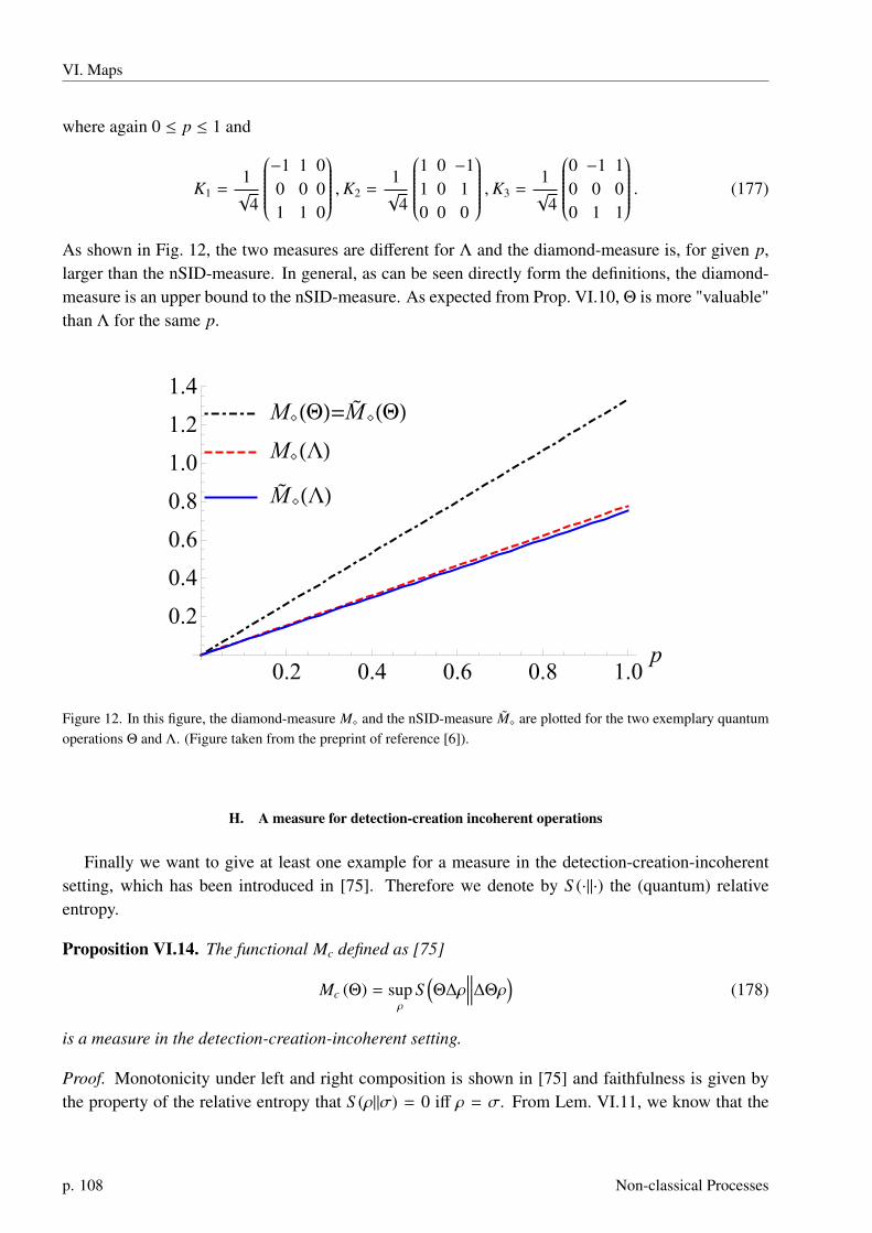
VI. Maps

where again 0 ≤ p ≤ 1 and

K1 =1√

4

−1 1 00 0 01 1 0

,K2 =1√

4

1 0 −11 0 10 0 0

,K3 =1√

4

0 −1 10 0 00 1 1

. (177)

As shown in Fig. 12, the two measures are different for Λ and the diamond-measure is, for given p,larger than the nSID-measure. In general, as can be seen directly form the definitions, the diamond-measure is an upper bound to the nSID-measure. As expected from Prop. VI.10, Θ is more "valuable"than Λ for the same p.

M⋄(Θ)=M⋄(Θ)

M⋄(Λ)

M⋄(Λ)

0.2 0.4 0.6 0.8 1.0p

0.2

0.4

0.6

0.8

1.0

1.2

1.4

Figure 12. In this figure, the diamond-measure M� and the nSID-measure M� are plotted for the two exemplary quantumoperations Θ and Λ. (Figure taken from the preprint of reference [6]).

H. A measure for detection-creation incoherent operations

Finally we want to give at least one example for a measure in the detection-creation-incoherentsetting, which has been introduced in [75]. Therefore we denote by S (·‖·) the (quantum) relativeentropy.

Proposition VI.14. The functional Mc defined as [75]

Mc (Θ) = supρ

S(Θ∆ρ

∥∥∥∥∆Θρ)

(178)

is a measure in the detection-creation-incoherent setting.

Proof. Monotonicity under left and right composition is shown in [75] and faithfulness is given bythe property of the relative entropy that S (ρ‖σ) = 0 iff ρ = σ. From Lem. VI.11, we know that the


H. A measure for detection-creation incoherent operations

eigenvectors of 1A ⊗ ∆B(ρA,B) are separable. For Γb(ρ) = ρ ⊗ |b〉〈b| and using joint convexity andcontractivity, we can then prove

Mc (Θ ⊗ 1) = supρ

S((Θ ⊗ 1)∆ρ

∥∥∥∥∆(Θ ⊗ 1)ρ)

= supρ

S(((Θ∆) ⊗ 1)(1 ⊗ ∆)ρ

∥∥∥∥((∆Θ) ⊗ 1)(1 ⊗ ∆)ρ)

= supσ=(1⊗∆)ρ

S(((Θ∆) ⊗ 1)σ

∥∥∥∥((∆Θ) ⊗ 1)σ)

= supqa|b,pb,|φa|b,b〉

S

((Θ∆) ⊗ 1)∑a,b

qa|b pb|φa|b, b〉〈φa|b, b|

∥∥∥∥∥∥((∆Θ) ⊗ 1)∑a,b

qa|b pb|φa|b, b〉〈φa|b, b|

≤ sup

qa|b,pb,|φa|b,b〉

∑a,b

qa|b pbS(((Θ∆) ⊗ 1)|φa|b, b〉〈φa|b, b|

∥∥∥∥((∆Θ) ⊗ 1)|φa|b, b〉〈φa|b, b|)

= sup|φ,b〉

S(((Θ∆) ⊗ 1)|φ, b〉〈φ, b|

∥∥∥∥((∆Θ) ⊗ 1)|φ, b〉〈φ, b|)

= sup|φ〉,b

S(ΓbΘ∆|φ〉〈φ|

∥∥∥∥Γb∆Θ|φ〉〈φ|)

≤ sup|φ〉

S(Θ∆|φ〉〈φ|

∥∥∥∥∆Θ|φ〉〈φ|)

≤ supρ

S(Θ∆ρ

∥∥∥∥∆Θρ)

=Mc(Θ). (179)

In addition, we have

Mc(Θ) = supρ

S(Θ∆ρ

∥∥∥∥∆Θρ)

= supρ

S(

TrB (((Θ∆) ⊗ 1) (ρ ⊗ |1〉〈1|))∥∥∥∥ TrB (((∆Θ) ⊗ 1) (ρ ⊗ |1〉〈1|))

)≤ sup

ρ

S(

((Θ∆) ⊗ 1) (ρ ⊗ |1〉〈1|)∥∥∥∥ ((∆Θ) ⊗ 1) (ρ ⊗ |1〉〈1|)

)= sup

ρ

S(

(Θ ⊗ 1) ∆ (ρ ⊗ |1〉〈1|)∥∥∥∥∆ (Θ ⊗ 1) (ρ ⊗ |1〉〈1|)

)≤ sup

ρ

S((Θ ⊗ 1)∆ρ

∥∥∥∥∆(Θ ⊗ 1)ρ)

=Mc (Θ ⊗ 1) (180)

and thus

Mc(Θ) = Mc(Θ ⊗ 1). (181)

PhD Thesis p. 109

VI. Maps

Convexity is given by

Mc

∑i

qiΘi

= supρ

S(∑

i

qiΘi∆ρ

∥∥∥∥∥∥∑i

qi∆Θiρ

)≤ sup

ρ

∑i

qiS(Θi∆ρ

∥∥∥∥∆Θiρ)

≤∑

i

qi supρ

S(Θi∆ρ

∥∥∥∥∆Θiρ)

=∑

i

qiMc(Θi). (182)

�


VII. CONCLUSION AND OPEN QUESTIONS

In this thesis we introduced a general framework that allows to analyse the role of non-classicalfeatures of quantum physics. The framework goes beyond the usual scope of quantum resource theo-ries in that it does not only focus on static properties, but can be used also in connection with dynamicproperties of maps or instruments or even multi-time statistics generated by measurements or instru-ments on a given dynamics. While the framework is very abstract, we have shown its applicationin three different settings. Namely to analyse the classicality of a given dynamics through the per-spective of a single non-degenerate measurement in chapter IV, to unify three different notions ofnon-classicality of states, namely entanglement, discord and coherence in chapter V, and to quantifythe amount of coherence a measurement can detect in chapter VI. The existence of a unifying frame-work for such different theories promises to yield further insights if it is used more extensively. Forinstance it seems possible to analyse Bell-type inequalities from the perspective of the framework.Another natural application could be to compare different types of quantum computation schemes, asthe framework is built to answer questions like how good a model can be simulated classically. Somefurther refinements might be necessary in this context. For instance a question that is important hereis what rôle memory plays, since a bigger memory will give the possibility to better simulate a model.We leave these questions open for future work and now focus on the different chapters, as each ofthem comes with its own physical insights.

In chapter IV we showed how one can link coherent properties of the propagators to the non-classicality of a given dynamics. One might be tempted to say that this is not new, as the coherenceone generates during an evolution are often used as witnesses of non-classicality. However, this roughintuition is not precise. Even if coherences are generated one might still be able to simulated the multi-time statistics classically. The crucial insight is that one needs not only to create coherences, but alsoto detect them, or they will not affect the statistics. On the other hand, even if no coherences aregenerated classical simulation might not be possible (for more details on these points see Ref. [7]).This is because in order for the propagators to have some physical meaning, one needs some additionalassumption of Markovianity. Most of chapter IV is devoted to detail what assumption is needed andwhy it is. Currently we are trying to generalize the results without assuming Markovianity, but ofcourse, in this case, the property cannot be defined on the propagators any more and we are studyingvarious reformulations.

In chapter V we generalised the resource theory of entanglement, Local Operations and ClassicalCommunications, to make it applicable to more general settings. This allowed us to connect differ-ent types of non-classicality, coherence, discord and entanglement, beyond quantifiers and measures,which recently has attracted considerable interest [47–49, 74, 77–79, 89–98]. While this is principallyof interest on a theoretical level, it may also provide insights that are relevant for the description ofexperimental quantum technologies. This becomes evident, for example, in considering the commu-nication of classical information via a physical channel. While this transfer is typically considered onan abstract mathematical level, treated completely independent of the physical set-up, a communica-tion channel is not an abstract notion, but a physical quantum system – a wire. Such a wire, ultimately,is quantum mechanical and the extent to which these quantum properties survive dictate its power asa communication channel and, importantly, its deviation from the idealised mathematical description

p. 112

of classical communication. To this end, having a clean way of how to treat resources in the wirecertainly helps to assess what can and cannot be achieved with such a wire and if the resources areused in an optimal way (or to meaningfully quantify the amount of lost resources in each step of theprotocol). For instance, we showed that in a simple quantum computation protocol we can link theprecision it can achieve with the coherence available. As a further application, it is straightforwardto adapt LOP to quantify non-classicality in open quantum systems if the environment can be probed(see the discussion at the end of subsection V B). We refer to the summary, on page 18 for links to ad-ditional details and applications, such as why it is possible to entangle two parties by sending particlesthat are not entangled with either, or insights into secret key distribution, multipartite entanglementor quantum discord. An interesting open question is if there is a one-to-one connection – such aswe established here in the bipartite case – between coherence and entanglement also in a multipartitesetting.

In chapter VI we focused particularly on the question how well a quantum operation can detectcoherence, which as seen in chapter IV is one of two necessary requisites for non-classical statistics.Interestingly, we found that the question cannot be approached by using the usual tool of resourcetheories of states. For this reason, we made a first step in a more general direction and constructed aformal resource theory on the level of operations using resource destroying maps [76]. We presentedtwo measures quantifying the ability of an operation to detect coherence. The first can be calculatedefficiently using a semidefinite program. The second, named the nSID-measure, can be evaluatedin an iterative manner and has a clear operational interpretation. Its value determines how well wecan distinguish the given quantum operation from the free operations in a single try. It seems clearthat this approach will also be useful in other settings than coherence theory, for instance wheneverthe question of the ability of measuring a property arises. The present approach will also be a goodstarting point for more general variants of resource theories.

PhD Thesis p. 113

VII. Conclusion

[1] D. Egloff, O. C. Dahlsten, R. Renner, and V. Vedral, “A measure of majorization emerging from single-shotstatistical mechanics,” New J. Phys. 17, 073001 (2015).

[2] M. García Díaz, D. Egloff, and M. B. Plenio, “A note on coherence power of n-dimensional unitary operators,”Quant. Inf. Comput. 16, 1282 (2016).

[3] J. M. Matera, D. Egloff, N. Killoran, and M. B. Plenio, “Coherent control of quantum systems as a resourcetheory,” Quantum Sci. Technol. 1, 01LT01 (2016).

[4] T. Theurer, N. Killoran, D. Egloff, and M. B. Plenio, “Resource theory of superposition,” Phys. Rev. Lett. 119,230401 (2017).

[5] D. Egloff, J. M. Matera, T. Theurer, and M. B. Plenio, “Of local operations and physical wires,” Phys. Rev. X 8,031005 (2018).

[6] T. Theurer, D. Egloff, L. Zhang, and M. B. Plenio, “Quantifying operations with an application to coherence,”Phys. Rev. Lett. 122, 190405 (2019).

[7] A. Smirne, D. Egloff, M. G. Díaz, M. B. Plenio, and S. F. Huelga, “Coherence and non-classicality of quantummarkov processes,” Quantum Sci. Technol. 4, 01LT01 (2018).

[8] T. Baumgratz, M. Cramer, and M. B. Plenio, “Quantifying coherence,” Phys. Rev. Lett. 113, 140401 (2014).[9] D. Frauchiger and R. Renner, “Quantum theory cannot consistently describe the use of itself,” Nat. Commun. 9, 1

(2018).[10] A. Einstein, B. Podolsky, and N. Rosen, “Can quantum-mechanical description of physical reality be considered

complete?” Phys. Rev. 47, 777 (1935).[11] J. S. Bell, “On the einstein podolsky rosen paradox,” Physics 1, 195 (1964).[12] J. S. Bell, “On the problem of hidden variables in quantum mechanics,” Rev. Mod. Phys. 38, 447 (1966).[13] A. Aspect, P. Grangier, and G. Roger, “Experimental tests of realistic local theories via bell’s theorem,” Phys. Rev.

Lett. 47, 460 (1981).[14] J. F. Clauser, M. A. Horne, A. Shimony, and R. A. Holt, “Proposed experiment to test local hidden-variable

theories,” Phys. Rev. Lett. 23, 880 (1969).[15] G. Weihs, T. Jennewein, C. Simon, H. Weinfurter, and A. Zeilinger, “Violation of bell’s inequality under strict

einstein locality conditions,” Phys. Rev. Lett. 81, 5039 (1998).[16] M. A. Rowe, D. Kielpinski, V. Meyer, C. A. Sackett, W. M. Itano, C. Monroe, and D. J. Wineland, “Experimental

violation of a bell’s inequality with efficient detection,” Nature 409, 791 (2001).[17] M. Ansmann, H. Wang, R. C. Bialczak, M. Hofheinz, E. Lucero, M. Neeley, A. D. O’Connell, D. Sank, M. Weides,

J. Wenner, A. N. Cleland, and J. M. Martinis, “Violation of bell’s inequality in josephson phase qubits,” Nature461, 504 (2009).

[18] B. Hensen, H. Bernien, A. E. Dréau, A. Reiserer, N. Kalb, M. S. Blok, J. Ruitenberg, R. F. L. Vermeulen, R. N.Schouten, C. Abellán, W. Amaya, V. Pruneri, M. W. Mitchell, M. Markham, D. J. Twitchen, D. Elkouss, S. Wehner,T. H. Taminiau, and R. Hanson, “Loophole-free bell inequality violation using electron spins separated by 1.3kilometres,” Nature 526, 682 (2015).

[19] D. Bohm, “A suggested interpretation of the quantum theory in terms of "hidden" variables. i,” Phys. Rev. 85, 166(1952).

[20] C. Rovelli, “Relational quantum mechanics,” Int. J. Theor. Phys. 35, 1637 (1996).[21] C. A. Fuchs and R. Schack, “Quantum-bayesian coherence,” Rev. Mod. Phys. 85, 1693 (2013).[22] N. D. Mermin, “Making better sense of quantum mechanics,” Rep. Prog. Phys. 82, 012002 (2019).[23] A. Acín, I. Bloch, H. Buhrman, T. Calarco, C. Eichler, J. Eisert, D. Esteve, N. Gisin, S. J. Glaser, F. Jelezko,

S. Kuhr, M. Lewenstein, M. F. Riedel, P. O. Schmidt, R. Thew, A. Wallraff, I. Walmsley, and F. K. Wilhelm, “Thequantum technologies roadmap: a european community view,” New J. Phys. 20, 080201 (2018).

[24] M. B. Plenio and S. Virmani, “An introduction to entanglement measures,” Quantum Inf. Comput. 7, 1 (2007).[25] R. Horodecki, P. Horodecki, M. Horodecki, and K. Horodecki, “Quantum entanglement,” Rev. Mod. Phys. 81, 865

(2009).


http://stacks.iop.org/1367-2630/17/i=7/a=073001

http://www.rintonpress.com/journals/qiconline.html#v16n1516

http://dx.doi.org/10.1088/2058-9565/1/1/01LT01

http://dx.doi.org/10.1103/PhysRevLett.119.230401


http://dx.doi.org/10.1103/PhysRevX.8.031005



http://dx.doi.org/10.1088/2058-9565/aaebd5


http://dx.doi.org/ 10.1038/s41467-018-05739-8

http://dx.doi.org/ 10.1038/s41467-018-05739-8

http://dx.doi.org/ 10.1103/PhysRev.47.777

http://dx.doi.org/ 10.1103/PhysicsPhysiqueFizika.1.195

http://dx.doi.org/ 10.1103/RevModPhys.38.447




http://dx.doi.org/ 10.1103/PhysRevLett.81.5039

https://doi.org/10.1038/35057215

https://doi.org/10.1038/nature08363


http://dx.doi.org/10.1038/nature15759

http://dx.doi.org/10.1103/PhysRev.85.166

http://dx.doi.org/10.1103/PhysRev.85.166

http://dx.doi.org/10.1007/BF02302261

http://dx.doi.org/10.1103/RevModPhys.85.1693



http://www.rintonpress.com/journals/qiconline.html



[26] C. H. Bennett and G. Brassard, “Quantum cryptography: Public key distribution and coin tossing,” in Proc. ofIEEE Int. Conf. on Comp., Syst. and Signal Proc., Bangalore, India, Dec. 10-12, 1984 (1984).

[27] V. Giovannetti, S. Lloyd, and L. Maccone, “Advances in quantum metrology,” Nat. Photonics 5, 222 (2011).[28] F. Haase J., A. Smirne, F. Huelga S., J. Kołodynski, and R. Demkowicz-Dobrzanski, “Precision limits in quantum

metrology with open quantum systems,” Quantum Measurements and Quantum Metrology 5, 13 (2018).[29] R. P. Feynman, “Simulating physics with computers,” Inter. Jour. of Theor. Phys. 21, 467 (1982).[30] P. W. Shor, “Polynomial time algorithms for prime factorization and discrete logarithms on a quantum computer,”

SIAM J. Sci. Statist. Comput. 26, 1484 (1997).[31] L. Henderson and V. Vedral, “Classical, quantum and total correlations,” J. Phys. A: Math. Gen. 34, 6899 (2001).[32] H. Ollivier and W. H. Zurek, “Quantum discord: A measure of the quantumness of correlations,” Phys. Rev. Lett.

88, 017901 (2001).[33] A. Datta, S. T. Flammia, and C. M. Caves, “Entanglement and the power of one qubit,” Phys. Rev. A 72, 042316

(2005).[34] K. Modi, A. Brodutch, H. Cable, T. Paterek, and V. Vedral, “The classical-quantum boundary for correlations:

Discord and related measures,” Rev. Mod. Phys. 84, 1655 (2012).[35] D. Braun, G. Adesso, F. Benatti, R. Floreanini, U. Marzolino, M. W. Mitchell, and S. Pirandola, “Quantum-

enhanced measurements without entanglement,” Rev. Mod. Phys. 90, 035006 (2018).[36] E. Schrödinger, “Die gegenwärtige situation in der quantenmechanik,” Naturwissenschaften 23, 807 (1935).[37] S. Kochen and E. P. Specker, “The problem of hidden variables in quantum mechanics,” in The Logico-Algebraic

Approach to Quantum Mechanics: Volume I: Historical Evolution, edited by C. A. Hooker (Springer Netherlands,Dordrecht, 1975) pp. 293–328.

[38] A. Peres, “Two simple proofs of the kochen-specker theorem,” J. Phys. A: Math. Gen. 24, L175 (1991).[39] A. Cabello, J. Estebaranz, and G. García-Alcaine, “Bell-kochen-specker theorem: A proof with 18 vectors,” Phys.

Lett. A 212, 183 (1996).[40] G. Kirchmair, F. Zähringer, R. Gerritsma, M. Kleinmann, O. Gühne, A. Cabello, R. Blatt, and C. F. Roos, “State-

independent experimental test of quantum contextuality,” Nature 460, 494 (2009).[41] A. J. Leggett and A. Garg, “Quantum mechanics versus macroscopic realism: Is the flux there when nobody

looks?” Phys. Rev. Lett. 54, 857 (1985).[42] A. J. Leggett, “Testing the limits of quantum mechanics: motivation, state of play, prospects,” J. Phys.: Condens.

Matter 14, R415 (2002).[43] C. Emary, N. Lambert, and F. Nori, “Leggett–garg inequalities,” Rep. Prog. Phys. 77, 016001 (2014).[44] G. Waldherr, P. Neumann, S. F. Huelga, F. Jelezko, and J. Wrachtrup, “Violation of a temporal bell inequality for

single spins in a diamond defect center,” Phys. Rev. Lett. 107, 090401 (2011).[45] A. Winter and D. Yang, “Operational resource theory of coherence,” Phys. Rev. Lett. 116, 120404 (2016),

1506.07975.[46] A. Streltsov, G. Adesso, and M. B. Plenio, “Colloquium: Quantum coherence as a resource,” Rev. Mod. Phys. 89,

041003 (2017).[47] A. Streltsov, U. Singh, H. S. Dhar, M. N. Bera, and G. Adesso, “Measuring quantum coherence with entangle-

ment,” Phys. Rev. Lett. 115 (2015).[48] E. Chitambar and M.-H. Hsieh, “Relating the resource theories of entanglement and quantum coherence,” Phys.

Rev. Lett. 117, 020402 (2016).[49] A. Streltsov, S. Rana, M. N. Bera, and M. Lewenstein, “Towards resource theory of coherence in distributed

scenarios,” Phys. Rev. X 7, 011024 (2017).[50] H.-P. Breuer and F. Petruccione, The Theory of Open Quantum Systems (Oxford University Press, 2002).[51] E. B. Davies and J. T. Lewis, “An operational approach to quantum probability,” Commun. Math. Phys. 17, 239

(1970).[52] G. Lindblad, “Expectations and entropy inequalities for finite quantum systems,” Commun. Math. Phys. 39, 111

(1974).

PhD Thesis p. 115

https://doi.org/10.1016/j.tcs.2014.05.025

https://doi.org/10.1016/j.tcs.2014.05.025

https://doi.org/10.1038/nphoton.2011.35

https://www.degruyter.com/view/j/qmetro.2018.5.issue-1/qmetro-2018-0002/qmetro-2018-0002.xml

http://dx.doi.org/10.1007/BF02650179

http://dx.doi.org/10.1137/S0097539795293172




http://dx.doi.org/10.1103/PhysRevA.72.042316




http://dx.doi.org/10.1007/BF01491891

http://dx.doi.org/10.1007/978-94-010-1795-4_17

http://dx.doi.org/10.1007/978-94-010-1795-4_17


http://dx.doi.org/ https://doi.org/10.1016/0375-9601(96)00134-X

http://dx.doi.org/ https://doi.org/10.1016/0375-9601(96)00134-X








http://arxiv.org/abs/1506.07975



https://link.aps.org/doi/10.1103/PhysRevLett.115.020403




http://dx.doi.org/10.1007/BF01647093

http://dx.doi.org/10.1007/BF01647093

http://dx.doi.org/10.1007/BF01608390

http://dx.doi.org/10.1007/BF01608390

VII. Conclusion

[53] F. A. Pollock, C. Rodríguez-Rosario, T. Frauenheim, M. Paternostro, and K. Modi, “Operational markov conditionfor quantum processes,” Phys. Rev. Lett. 120, 040405 (2018).

[54] G. Chiribella, G. M. D’Ariano, and P. Perinotti, “Theoretical framework for quantum networks,” Phys. Rev. A 80,022339 (2009).

[55] G. Chiribella, G. M. D’Ariano, and P. Perinotti, “Quantum circuit architecture,” Phys. Rev. Lett. 101, 060401(2008).

[56] G. Chiribella, G. M. D’Ariano, and P. Perinotti, “Transforming quantum operations: Quantum supermaps,” EPL(Europhysics Letters) 83, 30004 (2008).

[57] D. Tamascelli, A. Smirne, S. F. Huelga, and M. B. Plenio, “Nonperturbative treatment of non-markovian dynamicsof open quantum systems,” Phys. Rev. Lett. 120, 030402 (2018).

[58] V. Vedral, M. B. Plenio, M. A. Rippin, and P. L. Knight, “Quantifying entanglement,” Phys. Rev. Lett. 78, 2275(1997).

[59] M. Horodecki, P. Horodecki, and J. Oppenheim, “Reversible transformations from pure to mixed states and theunique measure of information,” Phys. Rev. A 67, 062104 (2003).

[60] J. Åberg, “Quantifying superposition,” arXiv:quant-ph/0612146 (2006).[61] G. Gour and R. W. Spekkens, “The resource theory of quantum reference frames: manipulations and monotones,”

New J. Phys. 10, 033023 (2008).[62] F. G. S. L. Brandão, M. Horodecki, J. Oppenheim, J. M. Renes, and R. W. Spekkens, “Resource theory of quantum

states out of thermal equilibrium,” Phys. Rev. Lett. 111, 250404 (2013).[63] V. Veitch, S. A. H. Mousavian, D. Gottesman, and J. Emerson, “The resource theory of stabilizer quantum com-

putation,” New J. Phys. 16, 013009 (2014).[64] A. Grudka, K. Horodecki, M. Horodecki, P. Horodecki, R. Horodecki, P. Joshi, W. Kłobus, and A. Wójcik,

“Quantifying contextuality,” Phys. Rev. Lett. 112, 120401 (2014).[65] L. Del Rio, L. Kraemer, and R. Renner, “Resource theories of knowledge,” arXiv:1511.08818 (2015).[66] V. Vedral and M. B. Plenio, “Entanglement measures and purification procedures,” Phys. Rev. A 57, 1619 (1998).[67] F. Levi and F. Mintert, “A quantitative theory of coherent delocalization,” New J. Phys. 16, 033007 (2014).[68] M. Horodecki, P. Horodecki, and R. Horodecki, “Separability of mixed states: necessary and sufficient conditions,”

Phys. Lett. A 223, 1 (1996).[69] B. M. Terhal, “Bell inequalities and the separability criterion,” Phys. Lett. A 271, 319 (2000).[70] G. Adesso, T. R. Bromley, and M. Cianciaruso, “Measures and applications of quantum correlations,” J. Phys. A:

Math. Theor. 49, 473001 (2016).[71] L. Kraemer and L. del Rio, “Currencies in resource theories,” 1605.01064v1.[72] X.-D. Yu, D.-J. Zhang, G. F. Xu, and D. M. Tong, “Alternative framework for quantifying coherence,” Phys. Rev.

A 94, 060302 (2016).[73] F. G. S. L. Brandão and G. Gour, “Reversible framework for quantum resource theories,” Phys. Rev. Lett. 115,

070503 (2015).[74] J. Ma, B. Yadin, D. Girolami, V. Vedral, and M. Gu, “Converting coherence to quantum correlations,” Phys. Rev.

Lett. 116, 160407 (2016).[75] S. Meznaric, S. R. Clark, and A. Datta, “Quantifying the nonclassicality of operations,” Phys. Rev. Lett. 110,

070502 (2013).[76] Z.-W. Liu, X. Hu, and S. Lloyd, “Resource destroying maps,” Phys. Rev. Lett. 118, 060502 (2017).[77] E. Chitambar and G. Gour, “Critical examination of incoherent operations and a physically consistent resource

theory of quantum coherence,” Phys. Rev. Lett. 117, 030401 (2016).[78] I. Marvian and R. W. Spekkens, “How to quantify coherence: Distinguishing speakable and unspeakable notions,”

Phys. Rev. A 94, 052324 (2016).[79] B. Yadin, J. Ma, D. Girolami, M. Gu, and V. Vedral, “Quantum processes which do not use coherence,” Phys. Rev.

X 6, 041028 (2016).[80] W. H. Zurek, “Quantum discord and Maxwell’s demons,” Phys. Rev. A 67, 012320 (2003).



http://dx.doi.org/ 10.1103/PhysRevA.80.022339










http://arxiv.org/abs/quant-ph/0612146

http://dx.doi.org/10.1088/1367-2630/10/3/033023




https://arxiv.org/abs/1511.08818



http://dx.doi.org/ https://doi.org/10.1016/S0375-9601(96)00706-2

http://dx.doi.org/ https://doi.org/10.1016/S0375-9601(00)00401-1



http://arxiv.org/abs/1605.01064v1















[81] M. Horodecki, P. Horodecki, R. Horodecki, J. Oppenheim, A. Sen(De), U. Sen, and B. Synak-Radtke, “Localversus nonlocal information in quantum-information theory: Formalism and phenomena,” Phys. Rev. A 71, 062307(2005).

[82] E. Knill and R. Laflamme, “Power of one bit of quantum information,” Phys. Rev. Lett. 81, 5672 (1998).[83] A. Datta, A. Shaji, and C. M. Caves, “Quantum discord and the power of one qubit,” Phys. Rev. Lett. 100, 050502

(2008).[84] P. W. Shor, “Algorithms for quantum computation: Discrete logarithms and factoring,” in Foundations of Computer

Science, 1994 Proceedings., 35th Annual Symposium on (IEEE, 1994) pp. 124–134.[85] S. Parker and M. B. Plenio, “Efficient factorization with a single pure qubit and logN mixed qubits,” Phys. Rev.

Lett. 85, 3049 (2000).[86] S. Parker and M. B. Plenio, “Entanglement simulations of shor’s algorithm,” J. Mod. Opt. 49, 1325 (2002).[87] P. W. Shor and J. Preskill, “Simple proof of security of the bb84 quantum key distribution protocol,” Phys. Rev.

Lett. 85, 441 (2000).[88] K. Horodecki, M. Horodecki, P. Horodecki, and J. Oppenheim, “Secure key from bound entanglement,” Phys.

Rev. Lett. 94, 160502 (2005).[89] Y. Yao, X. Xiao, L. Ge, and C. P. Sun, “Quantum coherence in multipartite systems,” Phys. Rev. A 92, 022112

(2015).[90] E. Chitambar, A. Streltsov, S. Rana, M. N. Bera, G. Adesso, and M. Lewenstein, “Assisted distillation of quantum

coherence,” Phys. Rev. Lett. 116, 070402 (2016).[91] A. Streltsov, E. Chitambar, S. Rana, M. N. Bera, A. Winter, and M. Lewenstein, “Entanglement and coherence in

quantum state merging,” Phys. Rev. Lett. 116, 240405 (2016).[92] X. Hu, A. Milne, B. Zhang, and H. Fan, “Quantum coherence of steered states,” Sci. Rep. 6, 19365 (2016).[93] X. Hu and H. Fan, “Extracting quantum coherence via steering,” Sci. Rep. 6, 34380 (2016).[94] M.-L. Hu and H. Fan, “Relative quantum coherence, incompatibility, and quantum correlations of states,” Phys.

Rev. A 95, 052106 (2017).[95] H. Zhu, Z. Ma, Z. Cao, S.-M. Fei, and V. Vedral, “Operational one-to-one mapping between coherence and

entanglement measures,” Phys. Rev. A 96, 032316 (2017).[96] C. Radhakrishnan, M. Parthasarathy, S. Jambulingam, and T. Byrnes, “Distribution of quantum coherence in

multipartite systems,” Phys. Rev. Lett. 116, 150504 (2016).[97] D. Girolami and B. Yadin, “Witnessing multipartite entanglement by detecting asymmetry,” Entropy 19 (2017).[98] K. Bu, L. Li, A. K. Pati, S.-M. Fei, and J. Wu, “Distribution of coherence in multipartite systems under entropic

coherence measure,” Preprint: arXiv (2017), 1710.08517v1.[99] T. S. Cubitt, F. Verstraete, W. Dür, and J. I. Cirac, “Separable states can be used to distribute entanglement,” Phys.

Rev. Lett. 91, 037902 (2003).[100] W. Dür, G. Vidal, and J. I. Cirac, “Three qubits can be entangled in two inequivalent ways,” Phys. Rev. A 62,

062314 (2000).[101] M. Walter, D. Gross, and J. Eisert, “Multi-partite entanglement,” Preprint: arXiv (2016), 1612.02437v2.[102] L. Lamata, J. León, D. Salgado, and E. Solano, “Inductive entanglement classification of four qubits under stochas-

tic local operations and classical communication,” Phys. Rev. A 75, 022318 (2007).[103] M. Backens, “Number of superclasses of four-qubit entangled states under the inductive entanglement classifica-

tion,” Phys. Rev. A 95, 022329 (2017).[104] J. I. de Vicente, T. Carle, C. Streitberger, and B. Kraus, “Complete set of operational measures for the characteri-

zation of three-qubit entanglement,” Phys. Rev. Lett. 108, 060501 (2012).[105] B. Regula, S. Di Martino, S. Lee, and G. Adesso, “Strong monogamy conjecture for multiqubit entanglement: The

four-qubit case,” Phys. Rev. Lett. 113, 110501 (2014).[106] E. Andersson, J. D. Cresser, and M. J. W. Hall, “Finding the kraus decomposition from a master equation and vice

versa,” J. Mod. Opt. 54, 1695 (2007).[107] S. Swain, “Master equation derivation of quantum regression theorem,” J. Phys. A: Math. Gen. 14, 2577 (1981).[108] P. Talkner, “The failure of the quantum regression hypothesis,” Ann. Phys. 167, 390 (1986).

PhD Thesis p. 117








http://dx.doi.org/ 10.1080/09500340110107207









http://dx.doi.org/ 10.1038/srep19365

http://dx.doi.org/10.1038/srep34380





http://dx.doi.org/10.3390/e19030124











http://dx.doi.org/ 10.1080/09500340701352581


http://dx.doi.org/ https://doi.org/10.1016/0003-4916(86)90207-1

VII. Conclusion

[109] J. Kofler and i. c. v. Brukner, “Condition for macroscopic realism beyond the leggett-garg inequalities,” Phys. Rev.A 87, 052115 (2013).

[110] L. Clemente and J. Kofler, “No fine theorem for macrorealism: Limitations of the leggett-garg inequality,” Phys.Rev. Lett. 116, 150401 (2016).

[111] W. Heisenberg, “Über den anschaulichen inhalt der quantentheoretischen kinematik und mechanik,” Zeitschrift fürPhysik 43, 172 (1927).

[112] C. A. Fuchs, “Qbism, the perimeter of quantum bayesianism,” 1003.5209v1.[113] B. P. Lanyon, M. Barbieri, M. P. Almeida, and A. G. White, “Experimental quantum computing without entangle-

ment,” Phys. Rev. Lett. 101, 200501 (2008).[114] M. Ali, “Quantum dissonance and deterministic quantum computation with a single qubit,” Int. J. Quantum Inf.

12, 1450037 (2014).[115] N. Killoran, F. E. S. Steinhoff, and M. B. Plenio, “Converting nonclassicality into entanglement,” Phys. Rev. Lett.

116, 080402 (2016).[116] B. Regula, M. Piani, M. Cianciaruso, T. R. Bromley, A. Streltsov, and G. Adesso, “Converting multilevel nonclas-

sicality into genuine multipartite entanglement,” New Journal of Physics 20, 033012 (2018).[117] J. Sperling, E. Agudelo, I. A. Walmsley, and W. Vogel, “Quantum correlations in composite systems,” J. Phys. B:

At., Mol. Opt. Phys. 50, 134003 (2017).[118] A. Streltsov, S. Rana, P. Boes, and J. Eisert, “Structure of the resource theory of quantum coherence,” Phys. Rev.

Lett. 119, 140402 (2017).[119] E. Chitambar, “Local quantum transformations requiring infinite rounds of classical communication,” Phys. Rev.

Lett. 107, 190502 (2011).[120] M. A. Nielsen and I. L. Chuang, Quantum Computation and Quantum Information, 1st ed. (Cambridge University

Press, 2000).[121] L. Roa, A. Delgado, and I. Fuentes-Guridi, “Optimal conclusive teleportation of quantum states,” Phys. Rev. A 68,

022310 (2003).[122] R. Bhatia, Matrix Analysis, Graduate Texts in Mathematics (Springer New York, 1996).[123] A. W. Marshall, I. Olkin, and B. C. Arnold, “Introduction,” in Inequalities: Theory of Majorization and Its

Applications (Springer, 2011).[124] M. A. Nielsen, “Conditions for a class of entanglement transformations,” Phys. Rev. Lett. 83, 436 (1999).[125] M. Lostaglio, “An introductory review of the resource theory approach to thermodynamics,” Reports on Progress

in Physics 82, 114001 (2019).[126] E. Ruch, “The diagram lattice as a structural principle,” Theor. Chim. Acta 38, 167 (1975).[127] M. Horodecki and J. Oppenheim, “Fundamental limitations for quantum and nano thermodynamics,” Nat. Com-

mun. 4 (2013), 10.1038/ncomms3059.[128] J. Åberg, “Truly work-like work extraction,” Nat. Commun. 4 (2013), 10.1038/ncomms2712.[129] G. Gour, M. P. Müller, V. Narasimhachar, R. W. Spekkens, and N. Y. Halpern, “The resource theory of informa-

tional nonequilibrium in thermodynamics,” Phys. Rep. 583, 1 (2015).[130] P. Faist and R. Renner, “Fundamental work cost of quantum processes,” Phys. Rev. X 8, 021011 (2018).[131] F. G. S. L. Brandão and M. B. Plenio, “Entanglement theory and the second law of thermodynamics,” Nat. Phys.

4, 873 (2008).[132] T. Theurer, A. Streltsov, and M. B. Plenio, “Stochastic coherence theory for qubits,” 1804.09467.[133] T. Biswas, M. García Díaz, and A. Winter, “Interferometric visibility and coherence,” Proc. Royal Soc. A 473,

20170170 (2017).[134] C. Napoli, T. R. Bromley, M. Cianciaruso, M. Piani, N. Johnston, and G. Adesso, “Robustness of coherence: An

operational and observable measure of quantum coherence,” Phys. Rev. Lett. 116, 150502 (2016).[135] M. Piani, M. Cianciaruso, T. R. Bromley, C. Napoli, N. Johnston, and G. Adesso, “Robustness of asymmetry and

coherence of quantum states,” Phys. Rev. A 93, 042107 (2016).[136] R. Jozsa, “Fidelity for mixed quantum states,” Journal of Modern Optics 41, 2315 (1994).[137] G. Vidal, “Entanglement monotones,” J. Mod. Opt. 47, 355 (2000).






http://dx.doi.org/10.1007/BF01397280

http://dx.doi.org/10.1007/BF01397280



http://dx.doi.org/10.1142/S0219749914500373

http://dx.doi.org/10.1142/S0219749914500373



http://dx.doi.org/10.1088/1367-2630/aaae9d









http://dx.doi.org/10.1007/978-0-387-68276-1_1

http://dx.doi.org/10.1007/978-0-387-68276-1_1


http://dx.doi.org/10.1088/1361-6633/ab46e5

http://dx.doi.org/10.1088/1361-6633/ab46e5

http://dx.doi.org/10.1007/BF01125896

http://dx.doi.org/ 10.1038/ncomms3059

http://dx.doi.org/ 10.1038/ncomms3059

http://dx.doi.org/10.1038/ncomms2712

http://dx.doi.org/ 10.1016/j.physrep.2015.04.003


http://dx.doi.org/10.1038/nphys1100

http://dx.doi.org/10.1038/nphys1100

http://arxiv.org/abs/1804.09467

https://dx.doi.org/10.1098/rspa.2017.0170

https://dx.doi.org/10.1098/rspa.2017.0170



http://dx.doi.org/10.1080/09500349414552171

http://dx.doi.org/10.1080/09500340008244048

[138] C. H. Bennett, H. J. Bernstein, S. Popescu, and B. Schumacher, “Concentrating partial entanglement by localoperations,” Phys. Rev. A 53, 2046 (1996).

[139] E. M. Rains, “Bound on distillable entanglement,” Phys. Rev. A 60, 179 (1999).[140] T. Hiroshima and M. Hayashi, “Finding a maximally correlated state: Simultaneous schmidt decomposition of

bipartite pure states,” Phys. Rev. A 70, 030302 (2004).[141] B. Dakic, V. Vedral, and i. c. v. Brukner, “Necessary and sufficient condition for nonzero quantum discord,” Phys.

Rev. Lett. 105, 190502 (2010).[142] K. Modi, T. Paterek, W. Son, V. Vedral, and M. Williamson, “Unified view of quantum and classical correlations,”

Phys. Rev. Lett. 104, 80501 (2010).[143] S. Hamieh, R. Kobes, and H. Zaraket, “Positive-operator-valued measure optimization of classical correlations,”

Phys. Rev. A 70, 052325 (2004).[144] R. Peck, C. Olsen, and J. L. Devore, Introduction to Statistics and Data Analysis 3th Edition (Cengage Learning,

2008).[145] Y. Huang, “Computing quantum discord is np-complete,” New J. Phys. 16, 033027 (2014).[146] M. B. Plenio and V. Vedral, “Bounds on relative entropy of entanglement for multi-party systems,” J. Phys. A:

Math. Gen. 34, 6997 (2001).[147] T.-C. Wei, “Relative entropy of entanglement for multipartite mixed states: Permutation-invariant states and dür

states,” Phys. Rev. A 78, 012327 (2008).[148] D. Janzing, P. Wocjan, R. Zeier, R. Geiss, and T. Beth, “Thermodynamic cost of reliability and low temperatures:

tightening landauer’s principle and the second law,” Int. J. Theor. Phys. 39, 2717 (2000).[149] M. Lostaglio, D. Jennings, and T. Rudolph, “Description of quantum coherence in thermodynamic processes

requires constraints beyond free energy,” Nat Comms 6, 6383 (2015).[150] S. D. Bartlett, T. Rudolph, and R. W. Spekkens, “Reference frames, superselection rules, and quantum informa-

tion,” Rev. Mod. Phys. 79, 555 (2007).[151] C. H. Bennett, D. P. DiVincenzo, C. A. Fuchs, T. Mor, E. Rains, P. W. Shor, J. A. Smolin, and W. K. Wootters,

“Quantum nonlocality without entanglement,” Phys. Rev. A 59, 1070 (1999).[152] M. A. Nielsen, C. M. Dawson, J. L. Dodd, A. Gilchrist, D. Mortimer, T. J. Osborne, M. J. Bremner, A. W. Harrow,

and A. Hines, “Quantum dynamics as a physical resource,” Phys. Rev. A 67, 052301 (2003).[153] J. Eisert, K. Jacobs, P. Papadopoulos, and M. B. Plenio, “Optimal local implementation of nonlocal quantum

gates,” Phys. Rev. A 62, 052317 (2000).[154] D. Collins, N. Linden, and S. Popescu, “Nonlocal content of quantum operations,” Phys. Rev. A 64, 032302

(2001).[155] C. Bennett, A. Harrow, D. Leung, and J. Smolin, “On the capacities of bipartite hamiltonians and unitary gates,”

Information Theory, IEEE Transactions on 49, 1895 (2003).[156] A. Mani and V. Karimipour, “Cohering and decohering power of quantum channels,” Phys. Rev. A 92, 032331

(2015).[157] Z. Xi, M. Hu, Y. Li, and H. Fan, “Entropic characterization of coherence in quantum evolutions,” arXiv:1510.06473

(2015).[158] K. Bu, A. Kumar, L. Zhang, and J. Wu, “Cohering power of quantum operations,” Phys. Lett. A 381, 1670 (2017).[159] K. Ben Dana, M. García Díaz, M. Mejatty, and A. Winter, “Resource theory of coherence: Beyond states,” Phys.

Rev. A 95, 062327 (2017).[160] C. L. Degen, F. Reinhard, and P. Cappellaro, “Quantum sensing,” Rev. Mod. Phys. 89, 035002 (2017).[161] B. Coecke, T. Fritz, and R. W. Spekkens, “A mathematical theory of resources,” Information and Computation

250, 59 (2016), quantum Physics and Logic.[162] Q. Zhuang, P. W. Shor, and J. H. Shapiro, “Resource theory of non-gaussian operations,” Phys. Rev. A 97, 052317

(2018).[163] M. García Díaz, K. Fang, X. Wang, M. Rosati, M. Skotiniotis, J. Calsamiglia, and A. Winter, “Using and reusing

coherence to realize quantum processes,” Quantum 2, 100 (2018).

PhD Thesis p. 119












http://dx.doi.org/ 10.1023/A%3A1026422630734

http://dx.doi.org/10.1038/ncomms7383

http://dx.doi.org/ 10.1103/RevModPhys.79.555






http://dx.doi.org/10.1109/TIT.2003.814935





http://dx.doi.org/ 10.1016/j.physleta.2017.03.022




http://dx.doi.org/10.1016/j.ic.2016.02.008

http://dx.doi.org/10.1016/j.ic.2016.02.008



http://dx.doi.org/10.22331/q-2018-10-19-100

VII. Conclusion

[164] E. Chitambar and G. Gour, “Comparison of incoherent operations and measures of coherence,” Phys. Rev. A 94,052336 (2016).

[165] E. Chitambar and G. Gour, “Erratum: Comparison of incoherent operations and measures of coherence [phys. rev.a 94, 052336 (2016)],” Phys. Rev. A 95, 019902 (2017).

[166] M. Horodecki and J. Oppenheim, “(quantumness in the context of) resource theories,” Int. J. Mod. Phys. B 27,1345019 (2013).

[167] A. Y. Kitaev, “Quantum computations: algorithms and error correction,” Russ. Math. Surv. 52, 1191 (1997).[168] J. Watrous, Theory of quantum information (Cambridge University Press, 2018).[169] A. Gilchrist, N. K. Langford, and M. A. Nielsen, “Distance measures to compare real and ideal quantum pro-

cesses,” Phys. Rev. A 71, 062310 (2005).[170] S. Boyd and L. Vandenberghe, Convex Optimization (Cambridge University Press, 2004).[171] J. Watrous, “Semidefinite programs for completely bounded norms,” Theory Comput. 5, 217 (2009).[172] M.-D. Choi, “Completely positive linear maps on complex matrices,” Linear Algebra Appl. 10, 285 (1975).[173] M. Jiang, S. Luo, and S. Fu, “Channel-state duality,” Phys. Rev. A 87, 022310 (2013).[174] W. Matthews, S. Wehner, and A. Winter, “Distinguishability of quantum states under restricted families of mea-

surements with an application to quantum data hiding,” Commun. Math. Phys. 291, 813 (2009).[175] D. Deutsch, “Quantum theory, the church–turing principle and the universal quantum computer,” Proc. R. Soc. A

400, 97 (1985).[176] D. Deutsch and R. Jozsa, “Rapid solution of problems by quantum computation,” Proc. R. Soc. A 439, 553 (1992).[177] K. Zyczkowski and I. Bengtsson, “On duality between quantum maps and quantum states,” Open systems & infor-

mation dynamics 11, 3 (2004).[178] D. C. Brody and L. P. Hughston, “Universal quantum measurements,” J. Phys. Conf. Ser. 624, 012002 (2015).





http://dx.doi.org/ 10.1142/S0217979213450197

http://dx.doi.org/ 10.1142/S0217979213450197

http://stacks.iop.org/0036-0279/52/i=6/a=R02


http://dx.doi.org/ 10.4086/toc.2009.v005a011

http://dx.doi.org/ 10.1016/0024-3795(75)90075-0


http://dx.doi.org/10.1007/s00220-009-0890-5

http://dx.doi.org/10.1098/rspa.1985.0070



http://dx.doi.org/ 10.1023/B:OPSY.0000024753.05661.c2

http://dx.doi.org/ 10.1023/B:OPSY.0000024753.05661.c2


Appendix A: Dynamical maps in finite dimensions

In this section we make a short introduction into dynamical maps. This is done to define thenotation used throughout the thesis. Mathematically, only knowledge of linear algebra on complexvector spaces is assumed here, but it is definitely not intended to be an introduction for quantumphysics.

The starting point is a finite dimensional Hilbert space, and we will always work in the represen-tation H = Cn, with the scalar product 〈u, v〉 =

∑i uivi. Identifying the vector space with the linear

function from the complex numbers to the vector space, we can also write 〈u, v〉 = u†v, where u† isthe adjoint of u (that is, u† is a linear map from the vector space to the complex numbers, with entriesgiven by the conjugate of the original vector u and hence an element of the conjugate dual vectorspace of the one of u). We mostly use the Dirac notation, which simply identifies |φ〉 with a purestate (a normalized vector φ) and 〈φ| with its adjoint. Then it makes sense to write the scalar productbetween φ and ψ as 〈φ|ψ〉 = φ†ψ.

As 〈φ|φ〉 = 1, we have that |φ〉〈φ|φ〉 = |φ〉 and we can identify the projector (that is a linear operatorΠ, with Π2 = Π) |φ〉〈φ|, acting on the Hilbert space H, with the vector |φ〉. We will also need mixedstates, that is, statistical mixtures of pure states. Due to the linearity of quantum mechanics, thesecan be conveniently written as ρ =

∑i pi|φi〉〈φi|, which results in positive Hermitian operators ρ = ρ†,

with trace 1, the set of states S (H). We can then identify (destructive) measurements with a collectionof adjoints of sub-normalised states {mi[·] = λi〈µi| · |µi〉 = Tr

[λi|µi〉〈µi| ◦ ·

]}i, with

∑i λi|µi〉〈µi| = 1,

such that one gets∑

i mi[|φ〉〈φ|] =∑

i λi|〈µi|φ〉|2 =

∑i λi〈φ|µi〉〈µi|φ〉 = 〈φ|φ〉 = 1. Indeed, up to

grouping measurement outcomes, any measurement (that is a multi-linear map from the state spaceto probability distributions) can be written in this way (this is a direct consequence of the positivityof the measurement). In the literature, one refers to

∑i λi, j|µi, j〉〈µi, j|, with

∑i, j λi, j|µi, j〉〈µi, j| = 1 as

positive operator valued measure (POVM). This directly leads to the definition of multipartite states.If one part of the system is pure, one would expect that one knows it as good as possible, whichmeans that the measurement outcomes should not depend on actions on the other parts. For instanceif one part is measured out, the description of the other part of the system should not change, if itwas fully known before. If this was not the case, you could disturb the measurement statistics inanother lab by doing measurements in your own. This would make it impossible to have independentexperiments. Fortunately, this is not possible in quantum mechanics. The requirement simply leadsto independent variables if the states on the two Hilbert spaces are pure and hence to the tensorproduct |φ〉〈φ|A ⊗ |ψ〉〈ψ|B = |φ〉A|ψ〉B〈φ|A〈ψ|B. Measuring part A with {mi}i and part B with {n j} j leads tomi[|φ〉〈φ|A]n j[|ψ〉〈ψ|B] with the rule above. The probability to get outcome j on part B conditioned ongetting the outcome i on part A is therefore n j[|ψ〉〈ψ|B], as if A was not there. A generic pure vector isa superposition of such vectors and hence

|φ〉AB =∑

i, j

φi, j|i〉A| j〉B.

A general state is the mixture of such states and hence can be written as ρAB =∑

i, j,k,l ρ(i, j);(k,l)|i〉〈k|A ⊗| j〉〈l|B. To get from a composite system to one part of it is given by measuring out one part andforgetting the outcome, which again can be easily checked to be independent of how one measures onepart. This leads to the partial trace, which, assuming (for simplicity) that {|k〉〈k|B}i is an orthonormal

p. 122

Appendix A. Dynamical maps in finite dimensions

basis of system B, is defined by TrB[ρAB] =∑

i, j,k,l ρ(i, j);(k,l)|i〉〈k|A.Suppose now, that one has an open system, of which one knows the initial state ρ (a trace one

operator on a Hilbert space, that is a probabilistic mixture of ), and assume it is initially uncorrelatedwith the environment. This makes sense for instance if one has no knowledge of the correlations andjust does this no-assumption. While one can learn details of the correlations through repeating theexperiment (similarly as one may learn about a magnetically controlled die through the statistics of itsoutputs), this corresponds to additional knowledge that in principle one has to model on a larger sys-tem, that in turn may initially be assumed to be uncorrelated with its environment. If one furthermoreassumes that the division between system and environment may change during the evolution, one hasto discard (trace out) a different environment at the end. The evolution of the system therefore willbe:

ρ 7−→ TrB′(VAB ◦ (ρA ⊗ τB) ◦ V†AB

)for some state τ of the initial environment B (possibly unknown and hence modelled statistically due tothe evolution) and some unitary evolution VAB (which either might be known due to some microscopicconstraints or modelled due to the evolution). Following the literature, we call such super-operators(that is, Hermitianity preserving maps from the set of operators on a given Hilbert space, to anotherset of operators possibly acting on a different Hilbert space) dynamical maps, channels or (due to theirproperties) completely positive and trace preserving operations. Purifying the environment B we get:

ρ 7−→ TrBC

((VAB ⊗ 1C) ◦ (ρA ⊗ |0〉〈0|BC) ◦ (VAB ⊗ 1C)†

)calling the total environment R and defining UAR = (VAB ⊗ 1C), we get:

ρ 7−→ TrR

(UAR ◦ (ρ ⊗ |0〉〈0|R) ◦ U†AR

)Writing out the trace explicitly

ρ 7−→∑

i

〈i|RUAR|0〉R ◦ ρA ◦ 〈0|RU†AR|i〉R

and defining KiA = 〈i|RUAR|0〉R we get to the Kraus-form:

ρ 7−→∑

i

KiA ◦ ρA ◦ (Ki

A)†

where obviously∑i

KiA†◦ Ki

A = 1.

Adding the identity a few times and reorganizing the scalar terms we arrive at the formulation as achannel:

ρ 7−→∑

a,a′,b,b′

∑i

|b〉〈b|Ki|a〉〈a|ρ|a′〉〈a′|(Ki)†|b′〉〈b′|

=∑

a,a′,b,b′

∑i

〈b|Ki|a〉〈a′|(Ki)†|b′〉〈a|ρ|a′〉|b〉〈b′|

=∑

a,a′,b,b′Λa;a′

b;b′〈a|ρ|a′〉|b〉〈b′|

p. 123


Where we defined:

Λa;a′

b;b′ =∑

i

〈b|Ki|a〉〈a′|(Ki)†|b′〉 =∑

i

〈b|Ki|a〉〈b′|Ki|a′〉

As such super-operators are tensors, it will turn out to be useful to use the abstract index conventionfor tensors (loosely following [177, 178]). As is standard, we use Latin indices for the elements of atensor in an explicit basis and Greek indices for the tensors themselves, making the space to whichthe tensors belong explicit.

A map (a linear map from the vector space of linear operators on a first Hilbert space to the vectorspace of linear operators on a second Hilbert space) in this notation is simply Λα;α′

β;β′ . Also we denotethe tensor product by Aα1;α2

α3;α4 ⊗ Bβ1;β2β3;β4

= (AB)(α1β1);(α2β2)(α3β3);(α4β4). Mα;α′ denotes a measurement (a linear map

from a vector space of linear maps on a Hilbert space to the real numbers), its dual Pα;α′ denotes apreparation (a linear map from the real numbers to the linear maps on the Hilbert space). If only oneindex exists on one line, we denote the missing one with an arrow, such that Pα′�

α� is a linear map onthe Hilbert space.

One could be tempted to go ahead and define 〈φ| = φ�α. However, while we will do that eventually,it is better to be a bit careful here. Remember that we defined 〈φ| such that it lies in the conjugate dualspace of |φ〉 = φα�, but we also have, by definition of the super-operators, that φα� lies in the dualspace of φα�. In formulas we have that

〈ψ|φ〉 = (ψ∗)α�φα�,

where we defined conjugation by its action on the elements (namely that they get complex conjugated((ψ∗)α�)i = (ψα�)i, which is independent of the basis chosen). What happened here is that the Diracnotation identifies the dual of the dual vector space with the vector space. Explicitly, it does notdistinguish between a preparation of a dual map (a map from the complex numbers to the maps fromthe Hilbert space to the complex numbers, such as φ�α) from a measurement (a map from the Hilbertspace to the complex numbers (ψα�) in our notation). In the abstract index notation we can work abit more explicitly (though, since we do work in finite dimensions, we will use the standard notationsin the main text) and define

·∗ :(Λα;α′β;β′ )

∗ := (Λ∗)β′;βα′;α = δ

ν′=β′

µ′=α′δβ=να=µ(Λ

∗)µ;µ′

ν;ν′ , (A1)

(Λ∗)b;b′a;a′ := Λb;b′

a;a′ , (A2)

where we also introduced the natural isomorphisms δ, whose action hopefully is obvious, but dependson the particular representation chosen for the indices (more details below). As a side-remark, thisyields for the concatenation of two channels

(Λβ;β′

α;α′Γγ;γ′

β;β′ )∗ = (Λ∗)α

′;αβ′;β (Γ∗)β

′;βγ′;γ = (Γ∗)β

′;βγ′;γ(Λ

∗)α′;αβ′;β , (A3)

which just means that conjugation reverses the time-ordering. We also define the transposition (map-ping a map from one Hilbert space to a second to a map from the dual of the second to the dual ofthe first) ψβ�Kα�

β�φα� = φα�(Kα�β� )Tψβ� = φα�(KT)β�α�ψβ� and similarly for the duals (we define

p. 124


everything relative to the underlying Hilbert spaces, not to the state spaces). Therefore

·T : (Λα;α′β,β′ )

T := (ΛT)β;β′

α,α′ = δβ=ν;β′=ν′

α=µ;α′=µ′(ΛT)µ;µ′

ν;ν′ , (A4)

(ΛT)a;a′

b;b′ := Λa;a′

b;b′ , (A5)

which means that one can usually safely forget about the transposition sign on the right-hand-side.Concatenation in this case yields

(Λβ;β′

α;α′Γγ;γ′

β;β′ )T = Λα;α′

β;β′ Γβ;β′

γ;γ′ = Γβ;β′

γ;γ′Λα;α′β;β′ , (A6)

which also reverses the action of the maps, but acts differently on the states.It is a good idea to choose first an orthonormal basis of the Hilbert space {biα�}i, which then

automatically gives the other bases using the conjugation and the transposition, where the action ofthe second depends on the order one chooses for the indices. For an expansion in bases (and hence toget the components of the tensor), we then get, starting from ψα� =

∑i ψibiα�,

ψα� = (ψα�)T =∑

i

ψibiα� (A7)

ψ�α = (ψα�)∗ =∑

i

ψibi�α (A8)

ψ�α = (ψα�)† =∑

i

ψibi�α, (A9)

where we defined ·† = (·∗)T, and hence:

·† : (Λα;α′β,β′ )

† :=((Λ∗)β′;βα′;α)T (A10)

=(Λ∗)α′;αβ′;β = δ

α′=γ′;α=γβ′=η′;β=η δ

η′=ν′

γ′=µ′δν=ηµ=γ(Λ

∗)µ;µ′

ν;ν′ (A11)

For the preparations Pα;β =∑

i, j Pi, jbiα�b j�β (and hence the states) one can consistently define theinner product ⟨

Aα;β|Bα′;β′⟩

=∑

i, j

Ai, jBi, j = (A∗)α;βBα;β = Tr[(Aα;β)† ◦ Bα′;β′],

where the trace is defined by (compare above)

Tr[Aα;β] := δα=βAα;β :=∑

i

(Aα;β)i,i =: Aα;α,

(identifying the linear map from the numbers to the states to the numbers with a number and hencealso its preparation, Aα;α, in the last equation). The concatenation is defined by

φ�α ◦ ψβ� = φ�αδβ=αψβ� = (φ∗)α�ψα� = 〈φ|ψ〉 (A12)

φα� ◦ ψ�β = φα�ψ�β = φα� ⊗ ψ�β = |φ〉〈ψ| (A13)

Aα;β ◦ Bγ;δ = Aα;βδγ=βBγ;δ =

∑i, j,k

Ai,kBk, j|i〉〈 j|α;δ (A14)

Λγ2;δ2α2;β2◦ Λ

α1;β1γ1;δ1

= Λγ;δα2;β2

Λα1;β1γ;δ . (A15)

p. 125


The rule is that whenever there are upper indices for the first map, the last equation is applied, other-wise, the second last. In our notation, we use concatenation after tensor products after direct productsand always right-to-left multiplication. In the main text we will generally not write abstract indicesin the notation which means we need to make tensor products and contractions explicit. On the otherhand, this makes it possible to drop the symbol for concatenation. Since that is the main function oneneeds in quantum mechanics, this choice is sensible. Doing so reduces our notation to the standardone. In this section we do not do this, to make the spaces and connections more explicit.

Finally we need to see how self-adjointness translates into this notation. Obviously one needs toidentify the dual vector space with the original vector space. For preparations (states) to be Hermitianor self-adjoint means:

Aα;α′ = (Aα;α′)† = (A∗)α′;α.

We also define the identity operator 1α′�α� by

1α′�α� φα′� = φα�

and more generally also for 1α;α′β;β′ ρα;α′ = ρβ;β′ .

With these conventions we can rewrite the above equation:

ρα;α′ 7−→ Λα;α′β;β′ ρα;α′ , (A16)

and due to

Λα;α′β;β′ ρα;α′ =

∑i

Kiα�β�ρα;α′(Ki†)�α′

�β′ =∑

i

Kiα�β�(Ki∗)�α′

�β′ρα;α′ ,

one gets

Λα;α′β;β′ =

∑i

Kiα�β�(Ki∗)�α′

�β′ ,

which shows clearly the connection between Kraus operators and super-operations.Next we re-derive necessary and sufficient conditions that a super-map Λ

β;β′

α;α′ is a channel.The condition that a linear map is a super-operator (i.e. that the final state is Hermitian, if the

initial state was), is given by:

Λα;α′β;β′ ρα;α′

!=

(Λα;α′β;β′ ρα;α′

)†=

((ρ∗)α

′;α(Λ∗)β′;βα′;α

)T= (Λ∗)α

′;αβ′;β (ρ∗)α′;α = (Λ∗)α

′;αβ′;β ρα;α′

Alternatively one can also argue that, since(Λα;α′β;β′ ρα;α′

)†only has the lower indices β, β′ and no upper

indices, we have that(Λα;α′β;β′ ρα;α′

)†= (Λ∗)α;α′

β′;β (ρ∗)α;α′ = (Λ∗)α;α′β′;β ρα′;α = (Λ∗)α

′;αβ′;β ρα;α′ ,

leading to the same result. From it follows that super-operators satisfy

Λα;α′β;β′

!= (Λ∗)α

′;αβ′;β =

(Λα;α′β;β′

)†, (A17)

p. 126


where, here and everywhere in the text, the dagger † refers to the conjugate transpose with respectto the underlying Hilbert space (implying that the Choi state of the map (see below) is self-adjoint),and not the adjoint of Λ on the state space, which would be

(Λα;α′β;β′

)†s= (Λ∗)β;β′

α;α′ . While the two waysto define the adjoint are related by an isomorphism, the spaces that are identified by the self-adjointproperty differ. For the inverse (if it exists), we have that

1α1;α′1α2;α′2

=

(Λα2;α′2β;β′

)−1Λα1;α′1β;β′ (A18)

=

(1α1;α′1α2;α′2

)†=

((Λα2;α′2β;β′

)−1)† (

Λα1;α′1β;β′

)†(A19)

and hence that if the original map was Hermitianity preserving, also its inverse is.The trace preserving criterion, which guarantees that the final states are normalised if the initial

were, is (by inspection):

Λα;α′β;β = δβ=β′Λα;α′

β;β′!= δα=α′

Further we note that there is an isometry between super-operators and Hermitian operators (theChoi-Jamiolkowsky isomorphism), defined by:

J[Λ](β,α′);(β′,α) = 1�µ�βδα′=ν′Λ

ν;ν′µ;β′δν=α

From equation (A17) it follows trivially, that Hermitian operators are mapped to Hermitianity pre-serving super-operators and vice versa. This isomorphism exchanges the order of the formerly upperindices, one gets it by identifying the preparation of a dual map with a measurement on the standardvector space and a preparation with a measurement on the dual vector space, that is, the complexconjugate of the conjugate vector spaces with the original vector space ((Λ∗)α;α′

β;β′ )∗ = Λ

β′;βα′;α ↔ Λα;α′

β;β′ ↔

Λ(αβ′);(α′β) ↔ Λα;�(α′β);β′ ↔ Λ

(αβ′)�(α′β)� ↔ Λ(α′β);(αβ′). Obviously there are many more. Note that the last three

are automatically identified in Dirac notation, as they simply are∑

a,b,a′,b′ Λa′,b,a,b′ |a′, b〉〈a, b′|. One getsalso the others if one adds a trace over the full expressions, Tr

[∑a,b,a′,b′ Λa′,b,a,b′ |a′, b〉〈a, b′|(·)

], which,

if one only considers the probabilities of experiments, that is, observable quantities, is always justi-fied. This the reason why Dirac notation is so useful and we will make extensive use of it in the maintext.

The complete positivity of a channel is a consequence of the concept that if one tensors the actionof two channels, it should still be a channel, i.e. positive Hermitian operators should be mapped topositive Hermitian operators. It is enough to have this for the map tensored with the identity (justwrite it out, to see this). Therefore the complete positivity is defined by:

∀A(αβ);(α′β′) ≥ 0 : Λα;α′γ;γ′1

η�β�A(αη);(α′η′)1

�η′

�β′ = Λα;α′γ;γ′ A(αβ);(α′β′) ≥ 0. (A20)

But this is equivalent to Tr2[J[Λ](γ,α′);(γ′,α) ◦A(αβ);(α′β′)] ≥ 0 . Since A(αβ);(α′β′) is a positive Hermitianoperator, it can be decomposed into

∑i φiαβ�φi�α′β′ , s.t. by linearity, the above is valid for any such

A exactly if

Tr2[J[Λ](γ,α′);(γ′,α) ◦ A(αβ);(α′β′)] = Tr2[J[Λ](γ,α′);(γ′,α) ◦ φαβ�φ�α′β′] = φ�α′β′ ◦ J[Λ](γ,α′);(γ′,α) ◦ φαβ� ≥ 0,

p. 127


for any φ. But due to the Schmidt-decomposition [120], one can always write φαβ� =∑

i ciµiα�νiβ�.Therefore, by linearity, the above factorises to the definition of positivity of J[Λ](γ,α′);(γ′,α). If onewould have instead chosen not to invert the upper indices, but just transpose them, one would needto use the transposed of A to get a condition for the resulting operator, but the transposed of A is notnecessarily positive, and one would not get such a simple condition.

The complete positivity of the map is therefore equivalent to:

J[Λ](β,α′);(β′,α) ≥ 0

Now it is useful to keep a fixed convention for how to store the information of the indices to see howthe different mappings act on the components. Commonly, though also not always, the convention isto use the first index for the kets. There are various ways in which one can do this, and unfortunatelythere is no standard. If the aim is to easily define the concatenation operation there are two naturalchoices. The first, which is the one we adopt in the main text, is to use

Λ~γ;~δ

~α;~β[[~a;~b;~c; ~d]] = Λ[[~a;~b;~c; ~d]] = Λ~c;~d

~a;~b,

such that the concatenation is simply the contraction of the last n index vectors with the first n ofthe subsequent object (after only having one remaining object on the right), followed by the tensorproduct of the remaining entries. Here, n = 2 if both the third and the fourth index vectors are non-zero, if this is not the case n = 1 if any of the second to fourth index vectors are non-zero, otherwisen = 0. This choice basically implements vector multiplication for the last n entry vectors with thefirst n entry vectors. An alternative choice would be to transpose the last two entries, but we do notgo into this here. With the choice above, the transposition acts as

ΛT[[~a;~b;~c; ~d]] = Λ[[~c; ~d;~a;~b]],

(note that with the convention chosen, ΛT[[~a;~b;~c; ~d]] =

(Λ~γ;~δ

~α;~β

)T[[~a;~b;~c; ~d]] , (ΛT)~γ;~δ

~α;~β[[~a;~b;~c; ~d]])

and the adjoint operation is

Λ†[[~a;~b;~c; ~d]] = Λ[[~b;~a; ~d;~c]] = ΛT[[~d;~c;~b;~a]].

The Choi state is given by

J[Λ][[~a;~b;~c; ~d]] = Λ[[~a; ~d;~b;~c]]

and the connection between Kraus operators and their corresponding channel is

Λ[[~a;~b;~c; ~d]] =∑

i

KicaKid

b,

which is a bit messy. If the basic object one works with are Kraus operators, it is therefore morestraightforward to adopt a different convention such as labelling first left upwards, then right upwards(Λ[[~a;~b;~c; ~d]] = Λ

~b;~d~a;~c). But then of course concatenation of channels gets messier. Another reasonable

choice is to use the natural ordering of the Choi state (Λ[[~a;~b;~c; ~d]] = Λ~d;~b~a;~c), which makes it easier to

check complete positivity, but concatenation gets very messy.

p. 128

Appendix B: Copyrights

This thesis contains material that was previously published in Refs. [3, 5, 7] and of the preprintof [6] (published after the submission of the thesis, but before its publication). The material is basedon the preprints of these publications and has been modified by the author for its presentation in thisthesis, as detailed in the text (in accordance with the author rights of IOP and APS). The copyrightslicenses of these references are:

Ref. [3]: Preprint: CC BY-NC-ND 3.0, Published version: c© 2016 IOP,Ref. [5]: CC BY 4.0,Ref. [7]: c© 2018 American Physical Society,Ref. [6]: c© 2019 American Physical Society.

p. 130

https://creativecommons.org/licenses/by-nc-nd/3.0/

https://creativecommons.org/licenses/by/4.0/

Documents

Non-Classical Processes in Quantum Mechanics