Embed Size (px)
Citation preview

Non-equilibrium dynamics of one-dimensional isolated
quantum systems
Ph.D. Thesis
Gergo Roosz
supervisor: Ferenc Igloi
Theoretical Physics Department, University of Szeged
Doctoral School of Physics
Wigner Research Center for Physics
Szeged, Hungary2017

ii
To Maria
iii
Szerzoi nyilatkozat
Kijelentem, hogy a doktori disszertaciomban foglaltak a 2. es a 3. fejezetek kivetelevel,
melyek az irodalomban fellelheto eredmenyeket tekintik at, sajat munkam eredmenyei, es
csak a hivatkozott forrasokat hasznaltam fel. Tudomasul veszem azt, hogy
disszertaciomat a Szegedi Tudomanyegyetem konyvtaraban, a kolcsonozheto konyvek
kozott helyezik el.

Contents
1 Introduction 1
2 Ground-state properties of quantum spin chains 5
2.1 Homogeneous transverse-field Ising chain . . . . . . . . . . . . . . . . . . . 7
2.2 Finonacci Ising quantum quasi-crystal . . . . . . . . . . . . . . . . . . . . . 9
2.2.1 Other quasi-periodic sequences defined by substitution . . . . . . . 10
2.2.2 Harris-Luck criteria . . . . . . . . . . . . . . . . . . . . . . . . . . . 12
2.3 Harper model . . . . . . . . . . . . . . . . . . . . . . . . . . . . . . . . . . 13
2.3.1 Aubry-Andre duality . . . . . . . . . . . . . . . . . . . . . . . . . . 13
2.4 Disordered quantum Ising chain . . . . . . . . . . . . . . . . . . . . . . . . 14
3 Quench dynamics of homogeneous systems 18
3.1 Numerical results on global quenches . . . . . . . . . . . . . . . . . . . . . 18
3.1.1 Magnetization . . . . . . . . . . . . . . . . . . . . . . . . . . . . . . 18
3.1.2 Entanglement entropy . . . . . . . . . . . . . . . . . . . . . . . . . 20
3.2 Quasi-classical description . . . . . . . . . . . . . . . . . . . . . . . . . . . 21
3.2.1 Correlation functions . . . . . . . . . . . . . . . . . . . . . . . . . . 23
3.2.2 Local magnetization . . . . . . . . . . . . . . . . . . . . . . . . . . 24
3.2.3 Entanglement entropy . . . . . . . . . . . . . . . . . . . . . . . . . 25
3.3 Spectra and the dynamical properties . . . . . . . . . . . . . . . . . . . . . 26
3.4 Experiments . . . . . . . . . . . . . . . . . . . . . . . . . . . . . . . . . . . 27
4 Local quenches 29
4.1 Introduction . . . . . . . . . . . . . . . . . . . . . . . . . . . . . . . . . . . 29
4.2 Model . . . . . . . . . . . . . . . . . . . . . . . . . . . . . . . . . . . . . . 30
4.3 Composite defect exponents . . . . . . . . . . . . . . . . . . . . . . . . . . 31
4.2 Scaling behavior in imaginary time . . . . . . . . . . . . . . . . . . . . . . 35
4.3 Scaling behavior in real time . . . . . . . . . . . . . . . . . . . . . . . . . . 36
4.4 Numerical investigations . . . . . . . . . . . . . . . . . . . . . . . . . . . . 37
4.4.1 Technical details . . . . . . . . . . . . . . . . . . . . . . . . . . . . 37
4.4.2 Ordered defect in the initial state . . . . . . . . . . . . . . . . . . . 38
4.4.3 Non-ordered defect in the initial state . . . . . . . . . . . . . . . . . 41
4.5 Discussion . . . . . . . . . . . . . . . . . . . . . . . . . . . . . . . . . . . . 44
iv

CONTENTS v
5 Quench dynamics of the Ising quantum quasi-crystal 45
5.1 The model . . . . . . . . . . . . . . . . . . . . . . . . . . . . . . . . . . . . 45
5.2 Entanglement entropy . . . . . . . . . . . . . . . . . . . . . . . . . . . . . 45
5.3 Local magnetization . . . . . . . . . . . . . . . . . . . . . . . . . . . . . . 47
5.4 Interpretation by wave packet dynamics . . . . . . . . . . . . . . . . . . . 50
5.5 Discussion . . . . . . . . . . . . . . . . . . . . . . . . . . . . . . . . . . . . 51
6 Quench dynamics of the Harper model 54
6.1 Quasi periodic XX-chain . . . . . . . . . . . . . . . . . . . . . . . . . . . . 54
6.2 Entanglement entropy . . . . . . . . . . . . . . . . . . . . . . . . . . . . . 55
6.3 Local magnetization . . . . . . . . . . . . . . . . . . . . . . . . . . . . . . 57
6.4 Semiclassical interpretation . . . . . . . . . . . . . . . . . . . . . . . . . . 57
6.5 Discussion . . . . . . . . . . . . . . . . . . . . . . . . . . . . . . . . . . . . 59
7 Nearly adiabatic dynamics of the Harper model 60
7.1 Kibble-Zurek scaling . . . . . . . . . . . . . . . . . . . . . . . . . . . . . . 60
7.2 Density of defects in the adiabatic dynamics . . . . . . . . . . . . . . . . . 62
7.3 Numerical results and scaling theory . . . . . . . . . . . . . . . . . . . . . 63
7.4 Discussion . . . . . . . . . . . . . . . . . . . . . . . . . . . . . . . . . . . . 66
8 Quench dynamics of the disordered Ising model 68
8.1 Introduction . . . . . . . . . . . . . . . . . . . . . . . . . . . . . . . . . . . 68
8.2 The model . . . . . . . . . . . . . . . . . . . . . . . . . . . . . . . . . . . . 69
8.2.1 Numerical calculation of time evolution . . . . . . . . . . . . . . . . 69
8.3 From fully ordered initial state to the ferromagnetic phase . . . . . . . . . 72
8.4 Quench to the critical point . . . . . . . . . . . . . . . . . . . . . . . . . . 73
8.4.1 Ferromagnetic initial state . . . . . . . . . . . . . . . . . . . . . . . 73
8.4.2 Paramagnetic initial state . . . . . . . . . . . . . . . . . . . . . . . 74
8.5 Discussion . . . . . . . . . . . . . . . . . . . . . . . . . . . . . . . . . . . . 78
9 Conclusion 79
10.Osszefoglalo 81
10.1. Bevezetes . . . . . . . . . . . . . . . . . . . . . . . . . . . . . . . . . . . . 81
10.2. Altalanosıtott lokalis kvencs . . . . . . . . . . . . . . . . . . . . . . . . . . 82
10.3. A Finonacci Ising kvazikristaly nem egyensulyi dinamikaja . . . . . . . . . 84
10.4. A Harper-modell nem egyensulyi dinamikaja . . . . . . . . . . . . . . . . . 86
10.5. Kozel adiabatikus dinamika a Harper modellben . . . . . . . . . . . . . . . 86
10.6. A rendezetlen Ising modell dinamikaja . . . . . . . . . . . . . . . . . . . . 87
10.7. Konkluzio . . . . . . . . . . . . . . . . . . . . . . . . . . . . . . . . . . . . 88
11 Acknowledgements 91

vi CONTENTS
A Time Evolution, Eigenstates 93
A.1 Transformation to quadratic form . . . . . . . . . . . . . . . . . . . . . . . 93
A.2 Solution of a general quadratic operator . . . . . . . . . . . . . . . . . . . 94
A.3 Solution of the homogeneous Ising chain . . . . . . . . . . . . . . . . . . . 95
A.4 Time evolution of the cl, c†l operators . . . . . . . . . . . . . . . . . . . . . 96
A.5 Majorana fermions . . . . . . . . . . . . . . . . . . . . . . . . . . . . . . . 98
B Quantities of interest 99
B.1 Magnetization . . . . . . . . . . . . . . . . . . . . . . . . . . . . . . . . . . 99
B.1.1 Definition . . . . . . . . . . . . . . . . . . . . . . . . . . . . . . . . 99
B.1.2 Calculation method . . . . . . . . . . . . . . . . . . . . . . . . . . . 99
B.2 Propagator . . . . . . . . . . . . . . . . . . . . . . . . . . . . . . . . . . . 101
B.3 Entanglement entropy . . . . . . . . . . . . . . . . . . . . . . . . . . . . . 102
B.3.1 Schmidt decomposition . . . . . . . . . . . . . . . . . . . . . . . . . 102
B.3.2 Definition of entanglement entropy . . . . . . . . . . . . . . . . . . 103
B.3.3 Properties of entanglement entropy . . . . . . . . . . . . . . . . . . 104
B.3.4 Calculation of entanglement entropy in spin chains . . . . . . . . . 105

Chapter 1
Introduction
Non-equilibrium relaxation in a closed quantum system following a change of some para-
meter(s) in the Hamiltonian is of recent interest, both experimentally and theoretically.
Considering the speed of variation of the parameter, we generally discriminate between
two limiting processes. For the quench dynamics, the parameter is modified instantan-
eously, which experimentally can be realized in ultra cold atomic gases [1–11] using the
phenomenon of Feshbach resonance. In this process the evolution of different observables
after the quench is of interest, as well as the possible existence and properties of the sta-
tionary state, in particular in integrable and non-integrable systems [12–57]. In the other
limiting relaxation process, in the so called nearly adiabatic dynamics the parameter is
varied very slowly, usually linearly in time with a rate 1/τ across a phase-transition point.
At the start of the process the system is in the ground state of the Hamiltonian. If the
variation of the Hamiltonian would be much slower than the time scale of the smallest gap,
the system would remain exponentially close to the instantaneous ground state. However
when the system reaches the critical point, the smallest gap goes to zero, and the variation
of the Hamiltonian cannot be slow enough to remain in the instantaneous ground state.
The question, how far is the described system from the instantaneous ground state, is
target of extensive investigations in the literature [50, 56,58–74].
We mention that the parameter in the Hamiltonian of a closed system can be driven
periodically or randomly in time, and the non-equilibrium dynamics of these driven systems
draws attention both experimental [75] and theoretical [76] [77].
Many results for quantum quenches have been obtained for homogeneous systems [12,
16–33, 50, 51, 55]; for example, the relaxation of correlation functions in space and in time
have generally an exponential form, which defines a quench-dependent correlation length
and a relaxation time. Many basic features of the relaxation process can be successfully
explained by a quasi-particle picture [38, 51, 56]: after a global quench quasi-particles are
created homogeneously in the sample and move ballistically with momentum dependent
velocities. The behavior of observables in the stationary state is generally different in
integrable and in non-integrable systems. For non-integrable models, thermalization is
expected [16–24, 50, 51] and the distribution of an observable is given by a thermal Gibbs
ensemble; however, in some specific examples this issue has turned out to be more complex
[25–27, 32]. By contrast, it was conjectured that stationary state averages for integrable
1

2 1. CHAPTER. INTRODUCTION
models are described by a generalized Gibbs ensemble [16], in which case each integral of
motion is separately associated with an effective temperature.
Concerning quantum quenches in inhomogeneous systems, there have been only a few
studies in specific cases; for example, entanglement entropy dynamics in random quantum
chains [78–80] and in models of many-body localization [81,82]. In some of these cases the
eigenstates are localized, which prevents the system from reaching a thermal stationary
state.
A special type of inhomogeneity, interpolating between homogeneous and disordered
systems, is a quasi-crystal [83, 84] or an aperiodic tiling [85]. Quasi-crystals are known to
have anomalous transport properties [86,87], which is due to the fact that in these systems
the long-time motion of electrons is not ballistic, but an anomalous diffusion described by
a power law. One may expect that the quasi-particles created during the quench have a
similar dynamical behavior, which in turn affects the relaxation properties of quasi-crystals.
Quasi-crystals of ultra cold atomic gases have been experimentally realized in op-
tical lattices by superimposing two periodic optical waves with different incommensurate
wavelengths. An optical lattice produced in this way realizes a Harper’s quasi-periodic
potential [88, 89], for which the eigenstates are known to be either extended or localized
depending on the strength of the potential. Different phases of the Bose-Hubbard model
with such a potential have been experimentally investigated [90,91]. There have also been
theoretical studies concerning the relaxation process in the Harper potential [92,93].
The dissertation is organized as follows: In chapter 2 the investigated quantities are
defined and the most important equilibrium properties of the investigated models are out-
lined. In chapter 3 some results about the after quench dynamics of spin chains from
the literature are recapitulated. These results will be referred and extended in the later
sections.
Our new results are presented in Chapters 4-8. Below we briefly summarize the main res-
ults from these Chapters.
In Chapter 4 the dynamics after a composite local quench is investigated. Composite
here means that not only one site was modified during the quench, but the local magnetic
fields on two neighboring sites and the coupling between them. The quench was done in
a quantum Ising chain, and a coupling and the two neighboring local magnetic field are
changed suddenly. We calculated the local magnetization on the quench site. A relation
with a 2D classical spin system was found, and using this relation a closed formula was
conjectured for the time evolution of the local magnetization. These closed formulas are
the main results of the chapter. We validated the formulas with precise numerical calcula-
tions using free-fermion techniques.
In Chapter 5 we investigated the after quench dynamics of the Fibonacci quasi-crystal.
The quantum Ising chain in its homogeneous version is perhaps the most studied model
for non-equilibrium relaxation [13–15,34–44,57,94]. We focus on the Fibonacci lattice, for
which many equilibrium properties of the quantum Ising model are known [95–101]. In this
chapter we investigated the after-quench dynamics of the magnetization and entanglement

3
entropy with numerical free-fermion calculations. We found, that the entanglement entropy
shows a power law increase after the quench, and the magnetization shows a stretched ex-
ponential increase. We also found a dynamical phase transition associated with the local
magnetization, which is not present in the homogeneous system. The results were inter-
preted with quasi-classical reasoning.
In chapter 6 the quench dynamic of the Harper model was investigated. In this model
there is a localization-delocalization transition, separating a localized phase and an ex-
tended phase. We investigated the dynamics of the entropy and the magnetization after
different quenches ending in the extended phase, at the critical point or in the localized
phase. We explored the functional form of the relaxation of the entanglement entropy and
the magnetization in the aforementioned quenches. We found, that both quanties remain
finite if the quench ends in the localized phase. If the quench ends in the extended phase
the behavior is strongly similar to the behavior of the homogeneous systems: The entangle-
ment entropy grows linearly, and the magnetization decrease exponentially. If the quench
ended at the transition point, the entanglement entropy grows as a power-law, and the
magnetization decreases with a starched exponential.
In chapter 7 we investigated a nearly adiabatic process in the Harper model by slowly
varying one of the parameters of the Hamiltonian, and the system is driven over the trans-
ition point. We investigated how far is the system from the instantaneous ground state
after crossing the localization-delocalization transition with finite speed. We present the
results of our large-scale numerical simulations, and give a modified version of the so-called
Kibble-Zurek scaling, which fits the numerical results well.
In chapter 8 we investigated the local magnetization after a global quench in a disordered
Ising chain. We explored the functional form of the relaxation of the local magnetization
with numerical free-fermion calculations. Two kinds of initial states were used in our calcu-
lations: one of these is ferromagnetic, in which all spins point in the X direction, the local
magnetization is 1. The other initial state is paramagnetic, in which all spins show in the
Z direction, and the local magnetization in the direction of the interaction (X-direction) is
zero.
The main results are: If the system after the quench is off-critical, the magnetization
remains finite. If the quench starts form the totally ferromagnetic phase, and ends in the
critical point, the magnetization shows an ultra slow decrease. If the quench start from
the totally paramagnetic state, and ends at the critical point, the magnetization increases,
which is a unique property of the disordered Ising chain: In all quenches performed in
homogeneous and quasi-periodic Ising chains the local magnetization always decreases.
There has been intensive investigations about the after quench dynamics of the entangle-
ment entropy in disordered spin chains [79–82]. The results about the magnetization are
in good agreement with these previous studies. At the end of the dissertation there is
an Appendix, in which detailed calculations are presented: the solution of the eigenvalue
problem of different spin chains; the calculation of the magnetization and the entanglement
entropy in spin chains; some facts about the ”meaning” of the entanglement entropy. The
dissertation is based on the following articles:

4 1. CHAPTER. INTRODUCTION
1. Ferenc Igloi, Gergo Roosz, Yu-Cheng Lin Nonequilibrium quench dynamics in quantum
quasicrystals New J. Phys. 15, 023036 (2013)
2. Ferenc Igloi, Gergo Roosz, Loic Turban Evolution of the magnetization after a local
quench in the critical transverse-field Ising chain J. Stat. Mech. (2014) P03023
3. Gergo Roosz., Uma Divakaran, Heiko Rieger, Ferenc Igloi Non-equilibrium quantum
relaxation across a localization-delocalization transition Phys. Rev. B 90, 184202
(2014)
4. Gergo Roosz, Yu-Cheng Lin, Ferenc Igloi Critical quench dynamics of random quantum
spin chains: Ultra-slow relaxation from initial order and delayed ordering from initial
disorder New J. Phys. 19, 023055 (2017)
Our related work about a randomly driven quantum Ising chain is: Gergo Roosz, Robert
Juhasz, Ferenc Igloi Nonequilibrium dynamics of the Ising chain in a fluctuating transverse
field Phys. Rev. B 93, 134305 (2016)
In the thesis the following abbreviations are used:
TIC Transverse-field Ising Chain
SDRG Strong Disorder Renormalization Group
RSRG-X Real-Space Renormalization Group for eXcited states
CFT Conformal Field Theory

Chapter 2
Ground-state properties of quantum
spin chains
In this Chapter we review the previously known ground-state properties of the models
studied in this work. We also list the definitions of the investigated quantities. The details
of calculation are presented in Appendix B.
The models investigated in this work are special cases of the inhomogeneous XY-model
H =1
2
L∑l=1
hlσzl +
1 + γ
2
L∑l=1
Jlσxl σ
xl+1 +
1− γ2
L∑l=1
Jlσyl σ
yl+1 . (2.1)
Here L is the number of spins, σzl and σxl are the Pauli matrices. Here ~ = 1 and the
parameters Jl and hl are dimensionless numbers. With the Jordan-Wigner transformation
[104] [105] the operator (2.1) can be written with fermion operators ck and c†k:
H = −L∑l=1
hl(c†l cl−1/2)−1 + γ
2
L−1∑l=1
Jl(c†l−cl)(c†l+1+cl+1)−1− γ
2
L−1∑l=1
Jl(c†l+cl)(cl+1−c†l+1)
+ JLw
[1 + γ
2(c†L − cL)(c†1 + c1) +
1− γ2
(c†L + cL)(c†1 − c1)
]e−iπ
∑Lj=1 c
†jcj (2.2)
Here w = 0 corresponds to the free boundary conditions, and w = 1 corresponds to
the periodic boundary conditions. The P = e−iπ∑Lj=1 c
†jcj parity operator commutes with
the Hamiltonian 2.2. One can diagonalize the Hamiltonian in the eigensubspaces of P .
P has two eigenvalues, +1 if the number of particles is even, and −1 if the number of
particles is odd. In the even subspace P = +1, in the odd subspace P = −1. In the
even and in the odd subspace the Hamiltonian is quadratic in the cl, c†l operators. The
ground state of Hamiltonian 2.2 is in the even subspace. With an appropriate Bogoliubov
transformation [196] new fermions (ηk and η†k) can be introduced
ηk =N∑i
(1
2(Φk(i) + Ψk(i))ci +
1
2(Φk(i)−Ψk(i))c
†i
), (2.3)
5

6 2. CHAPTER. GROUND-STATE PROPERTIES OF QUANTUM SPIN CHAINS
and with these new fermionic operators the (2.1) Hamiltonian is diagonal:
H =L∑k=1
εkη†kηk + const. . (2.4)
The Φk(i) and Ψk(i) quantities in equation (2.3) are real numbers. Their calculation, and
the details of this standard diagonalization technique can be found in Appendix A. For
later reference I define here the Majorana operators:
a2l−1 = cl + c†l (2.5)
a2l = i(cl − c†l ) , (2.6)
which are self adjoint operators, and often make calculations more simple. The Majorana
operators satisfies the following simple anti-commutation rule: al, ak = 2δl,k. The time
evolution of the Majorana operators after a sudden quench can be expressed in the form
am(t) =∑2L
n=1 Pm,n(t)an, where Pm,n(t) are real coefficients. The calculation of the Pm,n(t)
coefficients are detailed in Appendix A.5. One gets the inhomogeneous XX model with
transverse field with γ = 0:
HXX = −1
2
L∑n=1
(σxnσxn+1 + σynσ
yn+1)− 1
2
L∑n=1
hnσzn , (2.7)
here all of the couplings are 1, and the hn transverse field is inhomogeneous. With hn =
h cos(2πn√
5−12
)n one gets the Harper model, which is investigated in more detail in this
work. One gets the transverse-field Ising chain from Hamiltonian (2.2) with γ = 1:
HIsing = −1
2
L−1∑i=1
Jiσxi σ
xi+1 −
1
2
L∑i=1
hiσzi + wJLσ
xLσ
x1 . (2.8)
In this work, three variants of the Ising chain will be investigated: One nearly homogeneous
with a (generalized) local defect, a quasi-periodic, and a disordered where the magnetic
fields and the couplings are (independent) random numbers.
One of the investigated quantities is the local magnetization. The Ising model shows fer-
romagnetic order in the x direction if the transverse field is small enough. The most
straightforward choice to characterize the magnetic order would be the expectation value
of σx. However this expectation value in the ground-state is always zero because of sym-
metry reasons. One possible solution is to add an infinitesimally small symmetry breaking
field. One adds a longitudinal field b to the Ising Hamiltonian and investigates the magnet-
ization in the ground state of the modified Hamiltonian Hb = HIsing+bV with V =∑N
i=1 σxi
It can be shown [167] , that the magnetization in the b→ 0 limit can be calculated as the
off-diagonal matrix member of σl between the ground state of (2.8) denoted by |Ψ0〉, and
the excited state of (2.8) denoted by |Ψ1〉.
ml = limb→0〈σxl 〉 = 〈Ψ0|σxl |Ψ1〉 (2.9)

2.1. HOMOGENEOUS TRANSVERSE-FIELD ISING CHAIN 7
An other interesting quantity investigated in this work is the entanglement entropy. The
formal definition is as follows. One divides the investigated system to two parts A and B.
One consider the density matrix of the system, which is simply the projector made from
the state vector of the system: ρ = |Ψ〉〈Ψ|. The reduced density matrix of subsystem A is
defined by tracing out for the degrees of freedom of the B system.
ρA = TrBρ (2.10)
The reduced density matrix of the B subsystem is defined similarly ρB = TrAρ. The
entanglement entropy is defined as the von Neuman entropy of ρA or ρB:
S = TrAρA ln ρA = TrBρB ln ρB . (2.11)
The set of the non-zero eigenvalues of ρA and ρB are identical, this is the reason why
the second equality holds in the previous equation. More details on the definition of the
entanglement entropy, and the calculation method for spin chains are included in Appendix
B.3. In this work A is always the first l spins of the chain, and B is the other L− l spins.
The definition allow any kind of partition. The choice of two intervals is the most simple
and perhaps the most interesting.
2.1 Homogeneous transverse-field Ising chain
The homogeneous Ising chain is derived from (2.8) with setting all of the couplings to J
and all of the magnetic fields to h. The model is exactly solvable, one first transform it to
a fermion system with the Jordan-Wigner transformation (A.5) [104] than diagonalize it
with a Bogoliubov transformation [105] [106]. The steps of this calculation are outlined in
Appendix A.3. There is a quantum phase transition in the model, the transition point is
h = 1. For h < 1 there is a long-range order in the x direction which is characterized by
non-zero transverse magnetization ml. The h < 1 phase is ferromagnetic, and the h > 1
phase is paramagnetic.
The paramagnetic and the ferromagnetic phases are mapped to each other by the duality
transformation [107]. To see this, let us investigate the Ising model with periodic boundary
conditions ( w = 1 in equation (2.8)). One can define a new set of Pauli matrices:
τxi = σzi+1σzi
τ zi = Πm<iσxm
τ yi = −iτ zi τxi
. (2.12)

8 2. CHAPTER. GROUND-STATE PROPERTIES OF QUANTUM SPIN CHAINS
With these matrices the Hamilton operator takes the form:
HperiodicIsing = −1
2
L∑i=1
σxi σxi+1 −
h
2
L∑i=1
σzi =
= −1
2
L∑i=1
τ zi −h
2
L∑i=1
τxi τxi+1 =
= h
[−1
h
1
2
L∑i=1
τ zi −1
2
L∑i=1
τxi τxi+1
]. (2.13)
So the spectra of the Hamiltonians HperiodicIsing (h) and hHperiodic
Ising (1/h) is the same. If h is in
the ferromagnetic phase than 1/h is in the paramagnetic phase, the duality connect the
two sides of the critical point.
The most important correlation functions have been calculated in [106]. The long-range
limit of the XX correlation function (Cxr 〈σxi σxi+r〉) shows the phase transition spectacu-
larly. In the paramagnetic phase limr→∞Cxr = 0, there is no long range order. In the
ferromagnetic phase the long range limit is nonzero:
limr→∞
Cxr = (1− h2)1/4 . (2.14)
The ml transverse magnetization behaves similarly to the Cxr correlation function, non-zero
in the ferromagnetic phase, goes to zero approaching the critical point (ml = (1 − h2)β),
and zero in the paramagnetic phase. The magnetization exponent is β = 1/8.
Using the Cxr correlation function one can obtain the correlation length of the system. One
find [108] that the correlation function shows an asymptotic decrease Cxr ∼ exp(−r/ξ),
where the inverse of the correlation length is:
1
ξ=
√
Tπ
( 1h− 1)e−2(1/h−1)/T h < 1, T → 0
π4T2
h = 1
1− 1/h+√
Tπ
( 1h− 1)e−2(1/h−1)/T h > 1, T → 0
. (2.15)
At the critical point, the XX correlation function decays as a power law: Cxr ∼ 1/r1/4,
which defines the η = 1/4 critical exponent [106]. In equation (2.15) T is the temperature.
In the ground state (at zero temperature) one finds ξ = 1/(1 − 1/h) for h > 1, so the
critical exponent of the correlation length is ν = 1. Approaching the critical point from the
paramagnetic phase the smallest gap closes as ∆ ∼ (h−1) [107], so the dynamical exponent
of the model is z = 1. The entanglement entropy between two blocks of spins remains finite
in the L → ∞ thermodynamic limit both in the ferromagnetic and paramagnetic phases.
This behavior is a special case of the general ”area-law”: In a non-critical system the
entanglement entropy is proportional to the area between the two subsystem [109]. In the
critical point of the TIC, the entanglement entropy shows a totally different behavior, it
grows logarithmically [110]:
S = c/6 lnL . (2.16)

2.2. FINONACCI ISING QUANTUM QUASI-CRYSTAL 9
where c = 1/2 is the central charge of the corresponding conformal field theory [168]. The
logarithmic growth of the entanglement entropy is a typical property of one-dimensional
critical systems. In a finite system the entanglement entropy shows a maximum at the
critical point.
2.2 Finonacci Ising quantum quasi-crystal
The Finonacci Ising quasi-crystal is defined by the Hamiltonian:
H = −1
2
[∑i
Jiσxi σ
xi+1 + h
∑i
σzi
], (2.17)
( σxi and σzi are Pauli matrices at site i.) The couplings, Ji, are site dependent, and
parameterized as:
Ji = Jrfi , (2.18)
Here r > 0 is the amplitude of the inhomogeneity, r = 1 corresponds to the homogeneous
system, the smaller r correspond to the stronger inhomogeneity. The fi numbers are
integers taken from a quasi-periodic sequence, from the so-called Fibonacci sequence.
The interaction J in (2.18) is fixed with J = r−ρ, where
ρ = limL→∞
∑Li=1 fiL
= 1− 1
ω, (2.19)
is the fraction of units 1 in a very long (infinite) sequence.
The Fibonacci sequence is defined by the following algebraic expression :
fi = 1 +
[i
ω
]−[i+ 1
ω
], (2.20)
where [x] denotes the integer part of x, and ω = (√
5+1)/2. The sequence can alternatively
defined by a substitution rule
A → AB
B → A
The lengths of the possible realizations of the Fibonacci chain are Fibonacci numbers
(1,2,3,5 ...). The first few realizations are:
A
AB
ABA
ABAAB
(2.21)

10 2. CHAPTER. GROUND-STATE PROPERTIES OF QUANTUM SPIN CHAINS
One can get the (n + 1) string by copying the (n − 1)th string after the nth string. The
phase transition of the homogeneous model survive in the quasi-periodic one, there is a
ferromagnetic phase if h is smaller than a critical value, and there is a paramagnetic phase,
if h is bigger than the critical hc. The critical magnetic field can be calculated with Pfeuty’s
result [111]. Pfeuty investigated an inhomogeneous Ising chain (2.8) with inhomogeneous
couplings and magnetic fields. The smallest excitation becomes zero (the system is critical)
in an inhomogeneous Ising model if
ΠLi=1hi = ΠL
i=1Ji . (2.22)
This relation holds for arbitrary choice of the couplings and magnetic fields, so for every
type of inhomogeneity. In Hamiltonian (2.17) the parameters were selected such a way
that the critical point is hc = 1.
In the literature various types of quasi-periodic sequences have been defined with vari-
ous substitution rules [101] [112]. The Fibonacci sequence was found to be an irrelevant
perturbation in the transverse Ising model, which means, the critical properties (exponents)
are common with the homogeneous model.
2.2.1 Other quasi-periodic sequences defined by substitution
In this section some examples of quasi-periodic sequences are listed, and their basis prop-
erties are obtained.
1. Fibonacci sequence defined above in detail.
2. Thue-Morse sequence. The substitution rule is
A → AB
B → BA (2.23)
Starting with letter A the first few realizations are: A, AB, ABBA, ABBABAAB.
3. Period doubling sequence. The substitution rule is:
A → BB
B → BA (2.24)
Starting with letter B the first few realizations are: B, BA, BABB, BABBBABA.
4. The Rudin-Shapiro-sequence is defined using an alphabet of four letters A,B,C,D.

2.2. FINONACCI ISING QUANTUM QUASI-CRYSTAL 11
The substitution rule is:
A→ AB
B → AC
C → DB
D → DC
Starting with letter A the first few realizations are: A, AB, ABAC, ABACABDC.
Usually when the Rudin-Shapiro-sequence is investigated only two interaction strength
are used (J0 and J1), and each letter denotes two neighboring couplings:
A→ J0J0
B → J0J1
C → J1J0
D → J1J1
For example the string ABAC denotes the next set of couplings: J0, J0; J0, J1; J0,
J0; J1, J0.
A quasi-periodic sequence usually described by the asymptotic density of different inter-
actions, and the so-called wandering exponent (β), which characterizes the deviation of
the couplings from the average. More formally the wandering exponent is defined by the
following equation:L∑i=1
Ji − LJ ∼ Lβ , (2.25)
where J is the average coupling in the thermodynamic (L → ∞) limit. The asymptotic
density of the different letters, and the wandering exponent can be obtained investigating
the substitution matrix. We present this method on the Fibonacci sequence, and list the
results for the other sequences. Let us denote the string which substitutes A (B) with s(A)
(s(B)). For the Fibonacci chain s(A) = AB and s(B) = A. The number of the B letters
in s(A) is denoted by ns(A)B . The substitution matrix is defined as:
M =
(ns(A)A n
s(B)A
ns(A)B n
s(B)B
). (2.26)
For the Fibonacci chain:
M =
(1 1
1 0
). (2.27)
And the number of the A and B letters in the mth realization is:(n
(m)A
n(m)B
)=
(ns(A)A n
s(B)A
ns(A)B n
s(B)B
)(m−1)(n
(1)A
n(1)B
)(2.28)

12 2. CHAPTER. GROUND-STATE PROPERTIES OF QUANTUM SPIN CHAINS
The asymptotic density of letters are given by the components of the eigenvector of M
corresponding to it’s maximal eigenvalue. The wandering exponent is β = ln |λ1|ln |λ2| , where λ1
is the largest eigenvalue of M , and λ2 is the second largest eigenvalue of M . In the case of
the Rudin-Shapiro chain M is a 4 × 4 matrix. The results for the different sequences are
as follows:
1. In the Fibonacci sequence the density of A letters is ρA = 1/ω, the density of the B
letters is ρB = 1/ω2. The wandering exponent is β = −1.
2. For the Thue-Morse sequence ρA = ρB = 1/2 and β = −∞.
3. For the period doubling sequence ρA = 1/3, ρB = 2/3 and β = 0.
4. For the Rudin-Shapiro sequence ρ(J0) = ρ(J1) = 1/2 and β = 1/2.
2.2.2 Harris-Luck criteria
The Harris-Luck criteria classifies the different quasi-periodic sequences according to their
effect on the static critical behavior. The criteria can be obtained with the following
phenomenological argument. Let us consider a spherical region of the quasi periodic model
with radius R, and let’s denote this region with Ω. (In one dimension Ω is an interval
of length 2R.) Let’s denote the number of couplings in Ω by B(Ω), and the sum of the
couplings by Σ(Ω) =∑
i,j∈Ω Ji,j. The aforementioned two quantities are proportional to the
volume |Ω| of the region Ω, which is proportional to RD, where D is the spatial dimension
of the system. The average coupling J0 is defined as J0 = limR→∞Σ(Ω)/B(Ω). The J0
average coupling determines the hc critical field in the thermodynamic limit.
For a big but finite Ω region the deviation from the average is characterized by:
Σ(Ω)− J0B(Ω) ∼ RDβ , (2.29)
where β is the wandering exponent. The correlation length of the system is ξ, ξ ∼ δ−ν ,
where δ is the distance from the critical point. The typical difference of the J couplings
from J0 is:J − J0
J∼ Σ(Ω)− J0B(Ω)
B(Ω)∼ ξDβ
ξD= ξ−D(1−β) . (2.30)
We introduce the local control parameter δi which is given by δi ∼ Ji. The typical deviation
of the local control parameter is:
∆δi ∼ ξ−Dν(1−β) . (2.31)
The perturbation is irrelevant if ∆δi δ in the thermodynamic limit, which gives the
following criteria for the irrelevance:
Dν(β − 1) + 1 < 0 . (2.32)

2.3. HARPER MODEL 13
The above condition is called the Harris-Luck criteria. The criteria states, that in the
transverse Ising chain where D = 1 and ν = 1 the Fibonacci and the Thue-Morse sequence
are irrelevant perturbations, the period doubling sequence is a marginal perturbation, and
the Rudin-Shapiro is a relevant perturbation.
2.3 Harper model
The Harper-model [88], also called Aubry-Andre model [89], is a quasi-periodic version of
the XX-model. It’s Hamilton operator is:
H = −1
4
L∑n=1
(σxnσxn+1 + σynσ
yn+1)−
L∑n=1
hnσzn . (2.33)
Here hn = h cos(2πβn) with β =√
5−12
= 1/ω is the inverse of the golden mean, h is the
amplitude of the quasi-periodic modulation. The ω parameter is irrational, this makes the
system quasi-periodic. There is a localization-delocalization transition in the model [102],
the transition point is h = 1. For |h| < 1 the eigenstates are extended over the whole
system, for |h| > 1 the eigenstates are exponentially localized [89]. With the Jordan-Wigner
transformation, a set of fermionic operators (cl, c†l ) can be introduced (see Appendix A),
and the Hamiltonian takes the following form (which is a special case of equation 2.2):
H = −1
2
L∑n=1
(c†ncn+1 + c†n+1cn)− hL∑n=1
cos(2πβn)c†ncn , (2.34)
which was also the original form of the model introduced by Harper [88].
2.3.1 Aubry-Andre duality
Following Aubry and Andre [89] a new set of fermion operators (ck, c†k, k = 1 . . . L) are
introduced:
ck =1√L
∑n
exp(i2πkβn)cn (2.35)
which are eigenstates of the momentum operator with eigenvalue: k = kFn−1modFn, where
Fn is the n-th Fibonacci number and L = Fn. In terms of these the Hamiltonian is given
by:
H = −h2
L∑k=1
(c†kck+1 + c†
k+1ck)−
2
h
L∑k=1
cos(2πβk)c†kck
. (2.36)
Note that Eq.(2.36) is in the same form as that in Eq.(2.34), thus the Hamiltonian
satisfies the duality relation:
H(h) ∼ hH(1/h) . (2.37)
Here ∼ denotes, that the two Hamiltonians are similar: their spectrum is the same.

14 2. CHAPTER. GROUND-STATE PROPERTIES OF QUANTUM SPIN CHAINS
Through Eq.(2.37) the small h regime of the Hamiltonian, in which the eigenstates are
extended in real space are connected with the large h regime, in which the eigenstates have
extended properties in Fourier space, thus these are in real space localized. The localiza-
tion transition takes place at the self-duality point, thus the critical amplitude of the field
is hc = 1. For h > 1 the localized states have a finite correlation length, ξ, which is given
as [89]:
ξ =1
ln(h), h > 1 , (2.38)
for all eigenstates of H. We will use the h → ±∞ limits in Chapter 7. For large |h| the
φq,n quantities are given as:
φq,n = δn,nq , εq = −h cos(2πβnq), |h| 1 . (2.39)
2.4 Disordered quantum Ising chain
The disordered Ising chain is defined by the Hamiltonian:
H = −1
2
[L∑i=1
Jiσxi σ
xi+1 +
L∑i=1
hiσzi
]. (2.40)
Here Ji and hi are positive independent random numbers, selected from the distributions
π(Ji) and ρ(hi) respectively. It was found, that the critical behavior is universal, inde-
pendent form the concrete shape of the distribution in the thermodynamic limit [115].
In the numerical simulations (presented in Chapter 8 ) We used uniform distribution
over [0, 1] for π(Ji), and uniform distribution over [0, h] for ρ(hi). The results recapitulated
in this section are true for general selection of π(Ji) and ρ(hi).
Pfeuty’s result about the criticality of the Ising chain [111] also holds for one realization
of the disordered chain, so a concrete realization is critical if ΠLi=1(hi) = ΠL
i=1Ji (see equation
(2.22)), or equivalently∑L
i=1 ln(hi) =∑L
i=1 ln Ji. The distribution of the disordered chains
is called critical if the average of the logarithm of the local magnetic fields (hi) and the
average of the logarithm of the couplings (Ji) are equal:
lnh = ln J . (2.41)
Here the over line denotes the average over the probability distribution. Note, that with
our choice of parameters the system is critical with h = 1. If lnh > ln J the system is
paramagnetic if ln(h) < ln(J) the system is ferromagnetic. The distance of the critical
point is usually measured with the parameter, introduced by Fisher [115]:
δ =ln(h)− ln(J)
var(h) + var(J), (2.42)
where var(J) is the varience of the couplings, and var(h) is the variance of the magnetic
fields. The disordered Ising chain shows equilibrium properties which are rather different

2.4. DISORDERED QUANTUM ISING CHAIN 15
from the properties of the homogeneous or quasi-periodic models.
Investigating the local magnetization one finds, in the critical point the typical real-
izations gives negligible contribution to the average. The average is dominated by so-
called rare events, which has vanishing probability but gives O(1) contribution to the
average [115] [116].
An other remarkable property of the disordered Ising chain is the existence of the so-
called Griffiths phase [116]. This phase is region in the neighborhood of the critical point.
It is the region where in the ferromagnetic phase some rare samples can be paramagnetic,
and in the paramagnetic phase some rare samples can be ferromagnetic. I summarize here
the properties of the surface magnetization, and the low-lying excitations. The surface
magnetization is a good example for a rare-event dominated average, and the properties of
the low-lying excitations will be used in Chapter 8. The surface magnetization ms = m1
is related to the local transverse fields and couplings with a relatively simple formula [117]
[118] :
ms =
[1 +
L−1∑l=1
Πlj=1
(hjJj
)2]−1/2
, (2.43)
where hi and Ji are arbitrary positive real numbers. In the critical point, the typical value
of the magnetization is determined by the largest term of the sum in equation (2.43). The
typical value of the largest term is ∼ exp(constL1/2) so the typical value of the surface
magnetization is:
mtyps (L) ∼ exp(−const.L1/2) . (2.44)
The average surface magnetization shows a rather different behavior [14]. There are rare
realizations where the random variables εj = lnhjJj
behaves like a surviving walk. This
realizations has O(1) contribution to the average of the magnetization, and dominate the
average. The average magnetization is:
[ms]av(L) ∼ L−x(s)m x(s)
m = 1/2 . (2.45)
In the ferromagnetic phase close to the critical point the surface magnetization is: [ms]av(δ) ∼|δ|βs with βs = 1. The typical and the average correlations can be described with differ-
ent correlation lengths. From the finite size dependence of the surface magnetization one
obtains: ξ ∼ |δ|−ν with ν = 2. The typical correlations decay faster: ξtyp ∼ |δ|−νtyp with
νtyp = 1.
In the remaining of this section we summarize the basic properties of the low-lying excit-
ations of the disordered transverse Ising model. The lowest excitation energy is [98]:
ε1(L) ∼ msmsΠL−1i=1
hiJi, (2.46)
where ms and ms are the boundary magnetizations on the two ends of the chain.
In the critical point the order of magnitude of the lowest excitation is given by the boundary
magnetization, so
ε(δ = 0, L) ∼ exp[− constL1/2
]. (2.47)

16 2. CHAPTER. GROUND-STATE PROPERTIES OF QUANTUM SPIN CHAINS
The typical time scale is given by the inverse of the lowest excitation tr ∼ ε−1, and the
length scale in the neighborhood of the critical point is given by the system size (ξ ∼ L),
so the length and time scale is connected as:
ln τ ∼ ξΨ , (2.48)
where Ψ = 1/2 [115] [117] [103]. In the homogeneous and quasi periodic quantum Ising
chains a power law scaling connect the time and the length scale tr ∼ ξz with a finite z
dynamical exponent. The (2.48) equation is a sign of an ultra-slow dynamics, where the
dynamical exponent is formally infinite.
In the paramagnetic Griffiths phase, where δ > 0, and maxJ > minh there are rare
regions of size lrare where the local couplings are stronger than the local magnetic fields,
and the system is locally ferromagnetic. Note that the boundaries of the Griffiths phase
depends on the probability distribution of hi and Ji. For example with the box distributions
used in Chapter 8 and already mentioned after the definition of the model, the Griffiths
phase extends over the whole off-critical (ferromagnetic and paramagnetic) region. The
energy gap in the aforementioned locally ferromagnetic rare samples is exponentially small
in lrare: ε ∼ exp[−constlrare], so the relation between the length and the time scale is:
tr ∼ ξz , (2.49)
with a finite dynamical exponent z. This scaling relation is typical for the Griffiths phase
[119]. The dynamical exponent in the Griffiths phase is continuous function of the δ
parameter. The precise value of z is given by the positive root of the equation:[(J
h
)z]= 1 . (2.50)
In the ferromagnetic phase the lowest excitation is exponentially small. The dynamical
exponent is usually obtained from the second gap, and found to be the positive root of[(h
J
)z]= 1 . (2.51)
However, the exponentially small first gap is also interesting from the viewpoint of the
dynamics, as the reader will see it in chapter 8.
The eigenstates of the off-critical disordered Ising model are localized [115]. In the
critical system there is a finite localization length for every excitations with ε > 0, but
the localization length is divergent for ε → 0 [120] [115]. The equilibrium properties of
the random chain can be best understood with the strong disorder renormalization group
(SDRG), which was applied by Fisher [115] to the critical point of the model and later was
generalized to the Griffiths phase [116]. The SDRG is a real-space renormalization group
method where the decimation step is the elimination of the strongest of the couplings
and magnetic fields. It is possible to follow the transformation of the distribution of the
magnetic fields and couplings under the renormalization flow. From these distributions

2.4. DISORDERED QUANTUM ISING CHAIN 17
one can conclude exact results about the thermodynamic behavior.

Chapter 3
Quench dynamics of homogeneous
systems
The quench dynamic means, that the quantum system is in its ground state initially, and
an external parameter is changed instantaneously. With the new value of the external
parameter the initial ground state is not an eigenstate of the new Hamiltonian, and a non-
trivial time evolution starts. More formally let’s denote the Hamiltonian of the system with
H(h), where h is the external parameter. For t < 0 h = h0 and the system is prepared in
the ground state of H(h0). Let’s denote this initial state with |Ψ(0)0 〉. At t = 0 the value of
the external parameter is changed instantaneously to h 6= h0, and remain h for t > 0. The
wave vector of the system is
|Ψ(t)〉 = e−iH(h)t|Ψ(0)0 〉 . (3.1)
for t > 0. The |Ψ(0)0 〉 original state of the system is usually not eigenstate of the after-quench
Hamiltonian H(h), and a non-trivial dynamics starts after the quench.
Usually we use the Heisenberg picture. The operator of physical observable A evolves
in the Heisenberg picture as
AH(t) = eiH(h)tAe−iH(h)t . (3.2)
The expectation value of the A observable is calculated as 〈A〉 = 〈Ψ(0)0 |AH(t)|Ψ(0)
0 〉. A two
point correlation function can be calculated as CA,B(t1, t2) = 〈Ψ(0)0 |AH(t1)BH(t2)|Ψ(0)
0 〉 =
〈Ψ(0)0 |exp(iH(h)t1)Aexp(−iH(h)(t1−t2))Bexp(−iH(h)t2)|Ψ(0)
0 〉. The time evolution of the
most simple operators are written down in detail in Appendix A.
3.1 Numerical results on global quenches
3.1.1 Magnetization
In [37] the authors investigated the quantum Ising model. Here we recapitulate the main
numerical results about the dynamics of the magnetization (order parameter). For very
long times (t L) the magnetization reaches an asymptotic value in a finite system.( In
figure 3.1 this regime is not show. The oscillations which can be seen in figure 3.1 decay,
18

3.1. NUMERICAL RESULTS ON GLOBAL QUENCHES 19
and become negligible for very long times.) The magnetization is measured on the l th
site in a system of total length of L spins. We assume L/2 > l so the nearest boundary is
at the first spin. For times of the same order of magnitude of the system length, different
regimes can distinguished.
1. For short times (t L) the relaxation of the magnetization is exponential:
ml(t) ≈ A(t)exp(−t/τ) for t < tl . (3.3)
This regime can be seen in figure 3.1 in the left-bottom panel before the first min-
imum. The A(t) prefactor is O(1). It is found to be oscillating if the quench ends in
the disordered phase A(t) ∼ cos(at+b), and positive (A(t) ∼ cos(at+b)+c > 0) if the
quench ends in the ferromagnetic phase. This first regime ends after tl time. It was
found that tl = l/vmax, where vmax is the maximum group velocity 1 in the system.
In other words vmax is the time needed by the fastest possible signals to reach the
lth spin from the boundary. If the bulk of an infinite system is investigated,(L→∞and l→∞ with l/L = constant) only this first regime exist.
2. Quasi-stationary regime. This regime can be seen in the left upper panel of figure 3.1,
when the magnetization is measured far from the center of the chain. (The length of
the chain was L = 256 so the center is l = 128. If the measured spin is far from the
center, the quasi-stationary regime is long (see the curve corresponding to l = 16), if
the spin is closer to the center the quasi-stationary regime becomes shorter (see the
curve corresponding to l = 64), if the measured spin is in the middle of the chain
(l = 128) the quasi-stationary regime vanishes.)
In this regime the decrease of the magnetization is much slower than in the previous
one. This regime starts when the fastest quasi-particles starting from the closer
boundary reach the measured spin (tl), and ends when the quasi-particles starting
from the other end of the chain (Lth) spin reach the measured spin (time (L−l)/vmax).This regime holds for tl < t < T − tl where T = l/vmax.
If one investigates a half infinite system, so the L → ∞ limit with fixed l, the
magnetization remains forever in this stationary regime.
3. Reconstruction regime.
After time T − tl the magnetization starts to increase
ml(t) ∼ exp(t/τ ′) . (3.4)
This regime ends at time T , when the fastest signals has run over the whole chain.
4. After time T approximately periodic behavior starts with period T . This periodicity
is the result of repeating reflection of signals at the end of the chain.
1The group velocity is given by vk = ∂ε(k)∂k

20 3. CHAPTER. PREVIOUS RESULTS ON QUENCHES
-8
-6
-4
-2
0
0 400 800 1200
log
ml(t
)
t
l=16l=32l=48l=64l=80l=96
l=112l=128
-50
-40
-30
-20
-10
0
0 200 400 600
log
ml(t
)
t
l=16l=32l=48l=64l=80l=96
l=112l=128
0
5
10
15
0 100 200 300 400 500
Sℓ(t)
t
ℓ =32ℓ =64ℓ =128
0
10
20
30
0 100 200
Sℓ(t)
t
ℓℓ =32=64=128ℓ
Figure 3.1. Upper row: Magnetization dynamics after a quench from h0 = 0 to h = 0.5(left) and from h = 0.5 to h = 1.5 (right). Lower row: Entanglement entropy dynamicsafter a quench from h0 = 0 to h = 0.5 (left) and from h0 = 0.5 to h = 1.5 (right). Thegray curve is the result of the semiclassical calculation which is detailed in section 3.2.3This figure is based on figure 1. of [79].
3.1.2 Entanglement entropy
Numerical investigations about the dynamics of the entanglement entropy were done in [56]
and [122]. In this subsection the main numerical results about the after quench dynamics
are recapitulated. The entanglement between the block of the first l spins, and the other
L− l spins was calculated. The typical dynamics of entropy is shown in figure 3.1.
The dynamics can divided to different regimes (shown in figure 3.1, lower panel ),
similarly to the magnetization:
1. For t < l/vmax the entanglement entropy increase. The functional form is found to
be:
S = α(h, h0)t , (3.5)
the α(h, h0) prefactor depends on the pre- and afterquench magnetic fields.
2. There is an intermediate region
l/vmax < t < (L− l)/vmax , (3.6)
where the entanglement entropy remain nearly constant. In the L → ∞ limit with

3.2. QUASI-CLASSICAL DESCRIPTION 21
finite l this constant value is the asymptotic value (t → ∞) of the entanglement
entropy.
3. For
(L− l)/vmax < t < T = L/vmax (3.7)
the entropy decreases.
4. After t > T an approximately periodic oscillation begins with period T .
3.2 Quasi-classical description
The quasi-classical description was first applied by Sachdev and Young [123] for finite
temperatures in equilibrium. Later this type of description was modified to describe zero
temperature non-equilibrium dynamics [37] of the local magnetization and the correlation
functions and also has been used to interpret the dynamical entanglement entropy [122]
[56]. In this subsection we follow articles [37] and [122] and describe the dynamics of the
magnetization and the entanglement entropy with the use of quasi-particles.
The quasi-classical transition works best if the quench ends in the ferromagnetic phase
(h < 1), and additionally h is small, not too close to the critical point.
With zero transverse magnetic field the ground state is twofold degenerate |Ψ0〉 =
a| + + + · · ·+〉 + b| − − − . . . 〉 where |+〉 and |−〉 are eigenstates of |σx〉. The lowest
excitation is (L − 1) times degenerate: |n〉 = | + + + · · · + + − − − · · · − −−〉, here n is
the position of the domain wall (kink).
A small transverse magnetic field h > 0 destroys the degeneracy of the lowest lying
excitations. First order perturbation gives that the low lying excitations are Fourier trans-
formations of the |n〉 domain wall states.
|Φ(p)〉 =∑
an|n〉 (3.8)
where an =√
2/L sin(pn), εh(p) = 1−h cos(p) and p has L− 1 discrete values in the [0, π]
interval.
The low lying excitations are Fourier transformations of domain walls, so a wave packet
formed from them represents a moving domain wall. It is known that the group velocity
of a wave packet which is localized in momentum space around momentum p is
vp =∂εp∂p
=h sin p
εp. (3.9)
In the quasi-classical picture the quasi-particles are created at the moment of the quench
homogeneously in the chain with momentum dependent probabilities. After they have
been created, they move ballisticaly (with constant speed) and are reflected from the ends
of the chain. After their creation the quasi-particles are considered to move determinist-
ically. The Ising model (with arbitrary couplings and magnetic field) can be transformed
to free fermions, the details can be found in Appendix A. In particular the after-quench

22 3. CHAPTER. PREVIOUS RESULTS ON QUENCHES
Hamiltonian with magnetic filed h can be written with fermion operators ηk and η†k in the
following diagonal form:
H =∑k
ε(k)η†kηk; (3.10)
where k is the momentum, which is a quasi-continuous variable in a large system, and
εh(k) =√
(h− cos p)2 + sin2 p the excitation energies. The η operators are connected to
the c operators by tha following Bogoliubov transformation:
ηq = uqcq + ivqc†−q (3.11)
η†−q = ivqcq + uqc†−q , (3.12)
where uh(p) =√
(εh(p) + h− cos p)/(2εh(p)) and vh(p) =√
(εh(p)− (h− cos p))/(2εh(p))
The ground state of the after quench Hamiltonian is the vacuum of the η fermions, denoted
by |0〉, The ground state before the quench (denoted by Ψ0) can be expressed with the
ground state after the quench ( |0〉)
|Ψ0〉 = Πp
[Un + iVnη
†pη†−p
]|0〉 , (3.13)
where Vp = uh0(p)vh(p) − vh0(p)uh(p) and Up = uh0(p)uh(p) + vh0(p)vh(p), and defined
in detail in Appendix A.3. From (3.13) one can see, that the quasi-particles are created
in pairs with opposite momenta. (This is also required to fulfill the conservation of the
momenta.) The probability of the creation of a quasi-particle pair on a given site with
momenta p and −p is:
fp = 〈Ψ0|η†pηp|Ψ0〉 = V 2p , (3.14)
fp =1
2
[1− h0h− (h0 + h) cos p+ 1
εh0(p)εh(p)
]. (3.15)
The motion of the quasi-particle pairs is periodic with period time 2Tp = 2 Lvp
. The position
of the initially right moving quasi-particle is denoted by x1(t), the position of the initially
left moving quasi-particle is denoted by x2(t). If a quasi-particle pair start from x0 the left
moving particle reach the boundary at ta = x0/vp, the right moving quasi-particle reach
the left boundary at time tb = (L− x0)/vp. For t < Tp the positions of the quasi-particles
are:
x1(t) =
x0 + vpt for t ≤ tb
2L− x0 − vpt for tb < t ≤ Tp ,(3.16)
x2(t) =
x0 − vpt for t ≤ ta
vpt− x0 for ta < t ≤ Tp .(3.17)
The quasi-particles meet at t = Tp in L− x0. Between Tp and 2Tp another two reflections
happen, and at t = 2Tp the quasi-particles meet again, at the position of their creation, x0
and with the same direction of velocities as at the time of their creation. The quasi-particles
move periodically with 2Tp period.
When a quasi-particle passes a spin the spin is flipped in the X direction. The two
elements of the quasi-particle pair are correlated with each other, but the quasi-particles

3.2. QUASI-CLASSICAL DESCRIPTION 23
l
t
(r1, t1)
(r2,t2)
Figure 3.2. Quasi-particle trajectories after a global quench.
from different pairs (starting from different positions) are uncorrelated.
3.2.1 Correlation functions
The correlation functions are defined as:
C(r1, t1; r2, t2) = 〈Ψ0|σxr1(t1)σxr2(t2)|Ψ0〉 . (3.18)
The behavior of this correlations are interesting on its own right, however in this work I
include them, because they are used during the calculation of the local magnetization. The
motion of the quasi-particles after the quench is deterministic, but the creation process is
stochastic. To calculate the expectation value of correlation functions, one has to average
over the possible initial configurations of the quasi-particles.
With a given quasi-particle initial configuration C(r1, t1; r2, t2) is +1 if the traject-
ories intersect the (r1, t1; r2, t2) line even times, and −1 if the trajectories intersect the
(r1, t1; r2, t2) line odd times.
The probability, that the quasi-particles started from the same site intersect the line
(r1, t1; r2, t2) an odd number of times is denoted by Q(r1, t1, r2, t2).
The probability that for a given set of n sites the kinks passed odd times the (r1, t1; r2, t2)
line is:
C(r1, t1; r2, t2)
Ceq(r1, r2)=
L∑n=0
(−1)nQn(1−Q)L−nL!
n!(L− n)!= (1−2Q)L ≈ e−2Q(r1,t1;r2,t2)L . (3.19)
To calculate Q(r1, t1; r2t2) one has to average over the quasi-particle pairs with different
momenta between 0 and π:
Q(r1, t1; r2, t2) =1
2π
∫ π
0
dpfp(h0, h)qp(r1, t1; r2, t2) . (3.20)
In the previous equation qp(r1, t1; r2, t2) denotes the probability that the two traject-
ories of a quasi-particle pair (x1(t) and x2(t)) together intersect the line (r1, t1; r2, t2) odd

24 3. CHAPTER. PREVIOUS RESULTS ON QUENCHES
number of times. The qp probability can be calculated as the sum of the probabilities
qp(x0|r1, t1; r2, t2):
qp =1
L
∫ L
0
dx0qp(x0|r1, t1; r2, t2) , (3.21)
where qp(x0|r1, t1; r2, t2) denotes the probability that the quasi-particle pair which originally
started from x0 with momenta p intersects the line (r1, t1; r2, t2) together odd number of
times.
3.2.2 Local magnetization
The local magnetization can be expressed as the correlation function of the lth spin at time
t, and the lth spin at t = 0 with the condition that the spin is fixed initially (σxl = +1).
ml(t) = meql C|σxl (t=0)=+1(l, 0; l, t) (3.22)
The aforementioned quantities (q(t, l), qp(t, l)) take special, more simple form:
q(t, l) = Q|σxl (t=0)=+1(l, 0; l, t) (3.23)
q(t, l) =1
2π
∫ π
0
dpfp(h0, h)qp(t, l) (3.24)
qp(t, l) =1
L
∫ L
0
dx0qp(x0|t, l) . (3.25)
To calculate the local magnetization one has to evaluate qp(t, l).
for early times, when the reflections at the ends did not play a role, qp(t, l) is simply
proportional with the length of the region from where the quasi-particles could reach the
l th site. The first reflected quasi-particles reach the lth spin at t1 = l/vp, so for t < t1
qp(t, l) = 2vpt/L.
After the quasi-particles reflected from the left boundary (neighborhood of the first
spin) arrives, the qp(t, l) probability remains constant. This constant period remain until
the reflections from the right end did not arrive, so for t1 = l/vp < t < t2 = (L− l)/vp the
qp(t, l) probability is constant pq(t, l) = 2l/L.
When the quasi-particles reflected from the right end arrives at the investigated site l,
the qp(t, l) probability becomes to decrease, and it decreases until t = Tp = L/vp. At time
Tp the qp(t, l) probability becomes zero again.
qp(t, l) =
2vpt/L for t ≤ t1
2l/L for t1 ≤ t ≤ t2
2− 2vpt/L for t2 ≤ t ≤ Tp
(3.26)
Since after Tp time the quasi-particles reach their original position, qp is periodic with
period Tp:
qp(t+ nTp, l) = q(t, l) (n = 1, 2 . . . ) . (3.27)
The q function is not periodic, because the quasi-particle pairs with different momenta

3.2. QUASI-CLASSICAL DESCRIPTION 25
A B
b b
(1) (2)
Figure 3.3. The quasi-particle pair denoted by (1) gives no contribution to the entanglemententropy. The other quasi-particle pair denoted by (2) gives non-zero contribution to theentanglement entropy.
has different speed and different period time. In an half-infinite system, so in the limit of
L→∞ with l = const. the t2 time becomes formally infinite, and
qp(t, l) =
2vpt/L for t < t1
2l/L for t > t1 .(3.28)
The magnetization is in the L→∞ limit:
ml(t) = meql exp(−t 2
π
∫ π
0
dpvpfp(h0, h)Θ(l−vpt))exp(−l 2π
∫ π
0
dpfp(h0, h)Θ(vpt−l)) (3.29)
The relaxation time of the magnetization is:
τ−1mag(h0, h) =
2
π
∫ π
0
dpvpfp(h0, h) . (3.30)
3.2.3 Entanglement entropy
In this section the quasi-classical description of the after quench entanglement entropy, and
some analytical results about the entropy are summarized. From (3.13) it can be seen that
the quasi-particles from one pair are entangled, and quasi-particles from different pairs are
not entangled.
A quasi-particle pair gives non-zero contribution to the entanglement entropy between
blocks A and B if one member of the pair is in A and the other member is in B.
The contribution of one quasi-particle pair is
sp = −(1− fp) ln(1− fp)− fp ln fp . (3.31)
Summing up the contributions of all quasi-particle pairs one obtains the precise value of
the entanglement entropy, see figure 3.1 The summing up of the entropies of quasi particles
(equation 3.31) is straightforward in the L→∞ and l 1 limit.
Sl(t) =
t 1
2π
∫dpvpsp if t < l/vmax
l 12π
∫dpsp if t l/vmax ,
(3.32)
which corresponds to the exact results of [57]. In this limit (L → ∞ and l 1), there
is only an increasing regime, and a plateau regime. There are no oscillations, because the
quasi particles are reflected only from one end. The oscillations in finite systems (figure
3.1) are results of the interference of the quasi particles reflected from the opposite ends of

26 3. CHAPTER. PREVIOUS RESULTS ON QUENCHES
the system.
3.3 Spectra and the dynamical properties
Usually the spectra of the Hamiltonian (after the quench) determines the mean features of
the dynamics. This will be illustrated by examples. The spectra of the operators can be
divided to three classes [113]:
1. Absolutely continuous spectra. The spectra of the most homogeneous systems are
absolutely continuous. For example the spectra of the homogeneous Ising model or
the homogeneous XX model is absolutely continuous. However, there are inhomo-
geneous models with absolutely continuous spectra, for example the spectra of the
Harper model is absolutely continuous in its extended phase.
The models with absolutely continuous spectra usually have eigenstates extended
over the whole system. 2
2. The second type is the so-called singular continuous spectra. Such spectra shows a
fractal like behavior.
This type of spectra is observed in certain quasi-periodic systems: in the critical
point of the harper model [102] or in the Fibonacci quasi-crystal [113].
3. The third kind is the pure point spectra, which is typical for disordered systems
(disordered Ising chain [115], Anderson model with diagonal and off diagonal dis-
order [120] ).
There are quasi-periodic systems with pure point spectra, an example is defined by
a substitutionary rule in [121] and the Harper model in its localized phase is also has
pure point spectra.
Usually there is a finite localization length if the spectrum is pure point spectrum.
The energy-dependent localization length shows the spatial extension of the eigen-
states with the given energy. It can happen, that the localization length is finite
almost in the whole spectra, but becomes divergent at a special energy value. This
happens in the critical point of the disordered Ising chain [115] and in the off-diagonal
Anderson model [120]. 3
There are a vast of literature about the dynamics of systems with various types of spectrum.
The results of the numerical and exact investigations can be summarized as follows:
1. In the case of absolutely continuous spectra the dynamics is usually ballistic. Ballistic
here means that the ”signals” travel with constant velocity in the chain.
2It is naturally possible to create a Hermitian operator with absolutely continuous spectra and localizedeigenstates. For example one can consider the spectra of the homogeneous XX model, and a complete basisof localized eigenvectors. Then one define the operator as the eigenbasis is the aforementioned localizedcomplete set, and the spectra is the spectra of the XX model. However in simple physically inspired modelsthe absolutely continuous spectra is exist together with the extended eigenstates.
3The spectra of the one particle excitations of the disordered Ising chain and the set of the positiveeigenenergies of the off-diagonal Anderson model are identical.

3.4. EXPERIMENTS 27
2. If the spectra is singular continuous the dynamics is slower,the wave packets spread
as a power law. This was observed in the critical point of the Harper model [102]
and in the Fibonacci quasi-crystal.
3. If there is pure point spectrum, localization or extremely slow dynamic was found.
Here localization means that the wave packet reaches a finite width in an infinite
system, as in the localized phase of the Harper model. Ultra slow growth of the
entanglement entropy after a quench was found in the disordered Ising chain and for
other disordered models.
A qualitative explanation of the above results was developed by Thouless and Piechon in
their articles [128]. They investigated the typical variation of the energy levels (∆E) of
a one-dimensional system when the boundary conditions are changed. The ∆E energy
scale defines a time scale t∗ ∼ 1/∆E. A wave packet needs t∗ time to spread trough
the entire chain of length L. One gets the diffusion exponent of the wave packet with
the x2(t∗) ∼ (t∗)2 ∼ L2 relationship. In a model with absolutely continuous spectrum
the typical variation of energy levels is ∆E ∼ 1/L, which implies σ = 1. In a model
with pure point spectrum, ∆E ∼ 1/L and σ ∼ lnL/L ≈ 0. If the spectra is singular-
continuous, the relation between the variation of energy levels and the system size is more
complicated,∆E ∼ L−1/α, with various exponents α. Detailed investigations shows, that
the qth moment of a wave-packet starting form the i0th site behaves as x(q)(i0, t) ∼ tσ(i0,q),
where the exponent σ(i0, q) depends on the initial position i0.
3.4 Experiments
In the past two decades the experimental study of non-equilibrium quantum dynamics
become possible in systems of trapped ultra-cold atoms [12]. The gas of neutral atoms
(mostly alkali atoms) is cooled with subsequent methods. In a typical experiment the gas
is first cooled by laser cooling [129] and then trapped in a magnetic or magneto-optical
trap, and the trapped gas is cooled further by microwave evaporate cooling [130]. These
systems were the first realizations of a Bose-Einstein condensate of weakly interacting
particles, and the pioneers of this experiments Eric A. Cornell, Wolfgang Ketterle and
Carl E. Wieman has been awarded with the 2001 Nobel Prize in Physics for constructing
these experiments. The usual way of studying a trapped condensate is the time-of-flight
measurement: The trap is turned off instantaneously, and the atoms of the condensate ex-
tends ballistically. The extended atomic cloud is photographed later. Since the condensate
is located in a small volume, the velocity distribution can be obtained by time-of-flight
measurement [131]. Cooling and trapping fermions is also possible. however technically
even more challenging, since the thermalization during the evaporating cooling is slower
than in the bosonic case due to the exclusion principle [132].
The systems built from trapped cold atoms are well isolated from the environment and
can be considered as closed systems during the duration of experiments. The time scale
of the dynamics of these cold-atom systems is much longer than the usual time scales in

28 3. CHAPTER. PREVIOUS RESULTS ON QUENCHES
solid sates. The reason of the longer time scale, is the dilute nature of this systems. The
typical time scale is a few ms which makes possible to experimentally follow the dynamics.
The interaction strength (usually characterized by the s-wave scattering length) between
the trapped atoms is tunable with an external magnetic filed due to the Fresbach reson-
ance [133].
With the use of the so-called optical lattices [134] experimental realization of lattice mod-
els became possible. An optical lattice is formed by the interference of contra propagating
laser beams, which create an effective optical potential. Atoms can be trapped at the
minima of the optical potential. (The minima of the optical potential are actually maxima
of the light intensity.)
One of the most natural models emerging in optical lattices is the Bose-Hubbard model
and the Fermi-Hubbard model [135]. Even the monitoring of a single atom became possible
in Hubbard-like models [136]. Among investigating naturally emerging models in optical
lattices it is possible to simulate several solid-state-physics inspired models [137]. Ising and
XY models were engineered on triangular lattice [138]. The metal-insulator transition was
observed in the experimental realization of the Harper-model [139]. Disordered systems
were also realized in optical latices [137].
The quench dynamics of isolated systems were investigated in many experiments. Kinoshita
investigated [3] [4] the quench dynamics and the steady state of an effectively one-dimensional
system. It was found, that the system does not reach a thermal steady state in the ob-
tainable time regime, the system was close to the integrable Lieb-Luttinger model. The
nearly integrability may be the reason of the lack of the thermalization. Marc Cheneau and
his colleges investigated the spreading of correlations in a one dimensional Bose-Hubbard
model [10]. They demonstrated experimentally the light-cone-like spreading of the correl-
ations, which is characteristic in homogeneous systems, and has been used in Section 3.2.
Nearly-adiabatic dynamics was also investigated in systems of ultra-cold atoms. Weiler et
al. investigated a Bose gas, which was cooled below the BEC transition point [140]. They
demonstrated spontaneous forming of defects (vortices) during the process. Sadler et al. [6]
investigated a spinor Bose gas (87Rb). This system shows both magnetism and superfluid-
ity. They have driven this system over a quantum phase transition, and investigated the
density of ”generated defects”. Here defects refer to any difference from the ground state
of the instantaneous Hamiltonian.
A periodically driven interacting Harper model was studied recently [75]. The periodic
driving induce a delocalized regime in the phase diagram of the system.
These experiments with cold atoms draw attention on their own right. On the other hand,
these experiments lead to better understanding of solid state physics. Furthermore these
systems may serve as a hardware of quantum computing [139].

Chapter 4
Local quenches
4.1 Introduction
The non-equilibrium process after a sudden change of a parameter ”quench” at T = 0 is of
recent interest, and there were much attention paid to the [13–51,55–57] global quenches,
where the parameters are varied homogeneously in space.
The local quench is another interesting question, when parameters are modified locally
at a given site. Experimental realization of local quenches is X-ray [141] absorption
in metals. The theoretically most investigated systems in this field are the critical one-
dimensional systems.
For those systems, exact analytical results have been derived using conformal field
theory (CFT) [142,143].
In CFT one investigates the continuum limit of the model, where the system evolves
in a continuous two dimensional space-time (x, t). In this description the local quench
means the sudden change of a parameter at a given spatial (x) position, for example the
strength of the coupling at x = 0, changes from κ1 before the quench (t < 0) to κ2, after
the quench (t > 0). The expectation value of operators are calculated with path-integral
methods. These conformal methods usually work for appropriate boundary conditions:
κ = 0 (uncoupled half chains) or κ = ∞ (fixed local spin) and κ = 1, i.e., uniformly
coupled chain. Among other quantities the after quench entanglement entropy has been
studied by CFT ( [122,144–147]), after joining two initially independent systems (changing
from κ1 = 0 to κ2 = 1), the entropy grows logarithmically [142], and the prefactor of the
logarithm is universal S(t) = (c/3) ln t + const, it is one third of the central charge of the
CFT. In finite systems the entropy cannot grow without limit, in a system of length L the
entropy starts to grow for short times, but for long times it shows a periodic variation in
terms of t/L [143].
Various correlation functions and also the magnetization have been investigated with
CFT: the time (measured from the time of the quench ) and spatial (distance measured
from the site of the local quench) dependence is usually characterized by power laws [142],
and the exponents are combinations of bulk and surface static scaling dimensions. The
CFT predictions have been tested against numerical calculations in concrete models [94],
and good agreement has been found.
29

30 4. CHAPTER. LOCAL QUENCHES
There were studies about local quenches in non-conformally invariant systems. For
quenches ending in the ordered phase of the transverse Ising chain, a semiclassical de-
scription was applied [38], which has been verified by numerical simulations [94]. The
strong disorder renormalization group method was modified to describe the dynamics of
disordered systems [103] such as TIC (transverse Ising chain), and the entanglement en-
tropy [79, 82] and the full counting statistics was [80] investigated with this modified
renormalization group. In critical disordered systems, both quantities has an ultra slow
S(t) ∼ ln ln t time dependence, which was tested against numerical calculations.
In this section we study the time evolution of the local magnetization at the critical
point of the TIC, after a generalized local quench: The value of the local coupling and also
the value of the local fields are changed at the time of the quench t = 0. The static critical
behavior near a local defect in the TIC is non-universal, the scaling dimension of the local
magnetization continuously varies with the defect strength xi = xi(κi) [118,148–152]. Later
this question has been studied with various methods, S-matrix theory [153], , conformal
methods [154–159] and conformal field theory [160–162].
The ground state [122], [163–165] and the dynamical [122,166] entanglement entropy
across a defect also shows a similar behavior: the so-called effective central charge is a
prefactor of the entropy, and a continuous function of the defect parameters. It is expected,
that the non-equilibrium relaxation of the magnetization is also non-universal.
4.2 Model
I consider a critical TIC of length L with free boundary conditions and a defect at L/2.
The Hamiltonian of the system is
Hi=−1
2
[L−1∑n=1
σxnσxn+1+(Ji−1)σxL/2σ
xL/2+1+
L∑n=1
σzn+(hi1−1)σzL/2 + (hi2−1)σzL/2+1
]. (4.1)
The index i = 1, 2 refers to the values of the transverse fields hi1, hi2 and the coupling Ji,
before and after the quench at t = 0. In this chapter the after quench time dependence
of the local magnetization is in the focus of the interest. I follow the evolution of the
local magnetization at the defect, md(t) = mn=L/2(t). To investigate this generalized local
quench a two dimensional classical model is introduced in section 4.3. The imaginary time
version of the above described quench is in close relation with this classical model. The
imaginary time version of the quench is defined on the n-τ plane, where n is the number
of the spins, and τ is the imaginary time. The quench process investigated in the n − τplane corresponds to a two-dimensional (2d) classical critical Ising model with a composite
ladder defect at the center (see figure 4.1 for an illustration; the x axes corresponds to τ
and n corresponds to y ).
With the help of the two-dimensional classical model, exact results can be obtained for the
imaginary time version. This results are summarized in section 4.3.
The real time behavior is obtained by analytical continuation the imaginary time behavior
in section 4.3. To do this, we use previous exact results from the literature about special
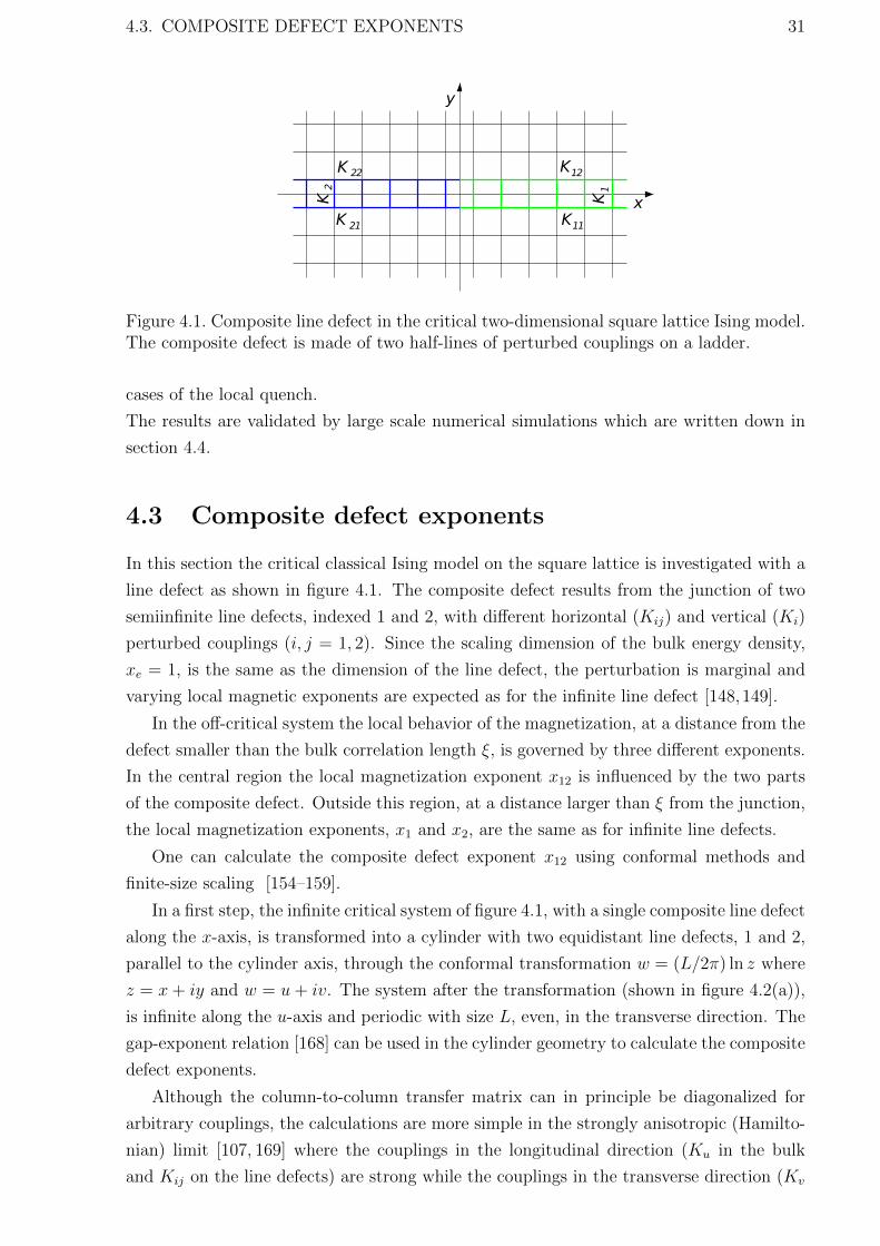
4.3. COMPOSITE DEFECT EXPONENTS 31
K2
22K
K 21
K12
K11
K1
x
y
Figure 4.1. Composite line defect in the critical two-dimensional square lattice Ising model.The composite defect is made of two half-lines of perturbed couplings on a ladder.
cases of the local quench.
The results are validated by large scale numerical simulations which are written down in
section 4.4.
4.3 Composite defect exponents
In this section the critical classical Ising model on the square lattice is investigated with a
line defect as shown in figure 4.1. The composite defect results from the junction of two
semiinfinite line defects, indexed 1 and 2, with different horizontal (Kij) and vertical (Ki)
perturbed couplings (i, j = 1, 2). Since the scaling dimension of the bulk energy density,
xe = 1, is the same as the dimension of the line defect, the perturbation is marginal and
varying local magnetic exponents are expected as for the infinite line defect [148,149].
In the off-critical system the local behavior of the magnetization, at a distance from the
defect smaller than the bulk correlation length ξ, is governed by three different exponents.
In the central region the local magnetization exponent x12 is influenced by the two parts
of the composite defect. Outside this region, at a distance larger than ξ from the junction,
the local magnetization exponents, x1 and x2, are the same as for infinite line defects.
One can calculate the composite defect exponent x12 using conformal methods and
finite-size scaling [154–159].
In a first step, the infinite critical system of figure 4.1, with a single composite line defect
along the x-axis, is transformed into a cylinder with two equidistant line defects, 1 and 2,
parallel to the cylinder axis, through the conformal transformation w = (L/2π) ln z where
z = x+ iy and w = u+ iv. The system after the transformation (shown in figure 4.2(a)),
is infinite along the u-axis and periodic with size L, even, in the transverse direction. The
gap-exponent relation [168] can be used in the cylinder geometry to calculate the composite
defect exponents.
Although the column-to-column transfer matrix can in principle be diagonalized for
arbitrary couplings, the calculations are more simple in the strongly anisotropic (Hamilto-
nian) limit [107, 169] where the couplings in the longitudinal direction (Ku in the bulk
and Kij on the line defects) are strong while the couplings in the transverse direction (Kv

32 4. CHAPTER. LOCAL QUENCHES
11h12h
h22
h21
J2
J 1
11
(b)
K1
K2
22K
K11
K12
K 21
K11
(a)
v
1
2
L/ 2
L−1
L
L/ 2+1
uL
h
Figure 4.2. (a) Under the conformal transformation w = (L/2π) ln z the full plane witha composite line defect becomes an infinite cylinder with circumference L and two infin-ite equidistant line defects, parallel to the cylinder axis. (b) In the extreme anisotropiclimit, the column-to-column transfer operator can be expressed as the exponential of theHamiltonian of a TIC, up to a rescaling factor.
in the bulk and Ki on the line defects) are weak. For a critical bulk in the extreme an-
isotropic limit, corresponding to a continuous imaginary time along the u-axis, the ratio
Kvc/K∗uc → 1 whereas on the line defects Ki/K
∗uc → Ji and K∗ij/K
∗uc → hij. Here K∗uc is
defined by the implicit equation tanhK∗uv = exp (−2Kuv).
Then the transfer operator is T = exp(−2K∗ucH) where H is the Hamiltonian of a
TIC [106] (see figure 4.2(b))
H = −1
2
[L∑n=1
σxnσxn+1 + (J1 − 1)σxLσ
x1 + (J2 − 1)σxL/2σ
xL/2+1
+L∑n=1
σzn + (h11 − 1)σzL + (h12 − 1)σz1 + (h22 − 1)σzL/2 + (h21 − 1)σzL/2+1
]. (4.2)
With the Jordan-Wigner transformation the Pauli spin operators σxn and σzn, are ex-
pressed in terms of fermion operators. [104] See details in Appendix A.4. The Hamiltonian
becomes quadratic in terms of fermion operators, but involves an operator P = (−1)Q, as-
sociated with the bond between the last (Lth) and the first spin.. The P operator commutes
withH, and its eigenvalues are +1 and −1 corresponding to Q = 0 and Q = 1. The number
of fermions is even (odd) if Q = 0 (Q = 1). In each subspace H(Q) is diagonalized by a
Bogoliubov transformation [106, 170] and takes the form H =∑
k εk
(η†kηk − 1
2
)in terms
of the new fermion operators ηk and η†k. One gets the square of the excitation energies as
the Q-dependent eigenvalues of the L × L matrix equation (M − ε2k) Φk = 0 with line n
(1 < n < L) given by:
h(n−1)J(n−1)Φk(n−1) + [h2(n)+J2(n−1)−ε2k]Φk(n)+h(n)J(n)Φk(n+1)=0. (4.3)

4.3. COMPOSITE DEFECT EXPONENTS 33
z
w=z2
y
x
v
u
(a)
(b)
Figure 4.3. The conformal transformation w = z2 maps the upper half-plane onto the fullplane with a cut along the positive real axis.
In lines 1 and L one has to replace J1 by (−1)Q+1J1. h(n) is the transverse field at site n
and J(n) the coupling between sites n and n+ 1 as shown in figure 4.2(b).
With ε2k = 4 sin2(k/2) and using the Ansatz
Φk(1) = −A , Φk(n) = (−1)n(B eikn + C e−ikn
)(n = 2, L/2) ,
Φk(L/2+1)= (−1)L/2+1D, Φk(n) = (−1)n(E eikn+F e−ikn
)(n = L/2+1, L), (4.4)
equation (4.2) becomes a linear system of six equations for the amplitudes A to F . The
characteristic equation gives the allowed values of k in each Q sector.
In the limit of large systems (continuum limit, 1/L→ 0), with εk = k = α/L, one can
expand the characteristic equation in powers of 1/L. To leading order, O (L−2), is found
to be
cosα =
[κ1 − (−1)Q κ2
]2 − [1 + (−1)Q κ1κ2
]2[κ1 − (−1)Q κ2]2 + [1 + (−1)Q κ1κ2]2
,
κi =Ji
hi1 hi2(i = 1, 2) , (4.5)
where κi is an effective bond interaction. This can be rewritten as
cot(α
2
)= ± κ1 − (−1)Q κ2
1 + (−1)Q κ1κ2
= − tan(α
2− π
2
). (4.6)

34 4. CHAPTER. LOCAL QUENCHES
By introducing the angle θi = arctan(1/κi) (i = 1, 2) one gets the relation
tan(α
2− π
2
)= ± tan θ1 − (−1)Q tan θ2
1 + (−1)Q tan θ1 tan θ2
= ± tan[θ1 − (−1)Q θ2
]. (4.7)
Thus the fermionic excitation energies take the form [157,159]
ε±r (Q) =2π
L(1/2±∆Q + r) , Q = 0, 1 , (4.8)
where r is an integer and
∆0 =
∣∣∣∣θ1 − θ2
π
∣∣∣∣ , ∆1 = 1− θ1 + θ2
π. (4.9)
One gets the magnetization exponent from the gap-exponent relation [168]
x12 =L
2π(Eσ − E0) , (4.10)
where E0 = E0(0) is the ground-state energy of H in equation (4.2 which belongs to the
even sector of the fermionic Hamiltonian whereas Eσ, which is the first excited state of H,
belongs to the odd sector. These two states belong to different sectors, so the gap involves
the difference ∆E between the ground-state energies in the two sectors and is given by
Eσ − E0 = ∆E + ε0(1) = E0(1)− E0(0) + ε0(1) , (4.11)
with [157]
∆E =2π
L
[1
2
(∆2
1 −∆20
)], ε0(1) = 1/2−∆1 . (4.12)
A simple expression for the local magnetization exponent is obtained by collecting the
above results:
x12 =2
π2arctan
(1
κ1
)arctan
(1
κ2
)=√x1x2 . (4.13)
This result can be proven for the “composite defect” shown in figure 4.3(b) where κ1 = 0
(cut on the positive u-axis) and κ2 = 1 (no perturbation around the negative u-axis).
Then x1 is the free surface exponent xms = 1/2, x2 the bulk exponent xm = 1/8 and from
equation (4.13) one gets x12 = 1/4. Now the conformal transformation w = zω/π is applied
to the critical upper half-plane of figure 4.3(a). The result of the conformal transformation
is a corner with opening angle ω and corner exponents are related to the surface exponents
via xc = πxms/ω [171,172]. If ω = 2π, the transformed system is the full plane with a cut
(see figure 4.3(b) ) so that x12 = xms/2 = 1/4.
The gap giving the local energy density exponent is Eε − E0, where Eε is the lowest
eigenstate of H with two fermions. Both states contains even fermions so that, according

4.2. SCALING BEHAVIOR IN IMAGINARY TIME 35
to equation (4.8), the local energy exponent, given by
L
2π(Eε − E0) =
L
2π
[ε−0 (0) + ε+0 (0)
]= 1 , (4.14)
keeps its unperturbed value. It is necessary to keep a truly marginal behavior for the local
magnetization when the defect strength is modified. Otherwise the criterion of marginality
would no longer be satisfied.
4.2 Scaling behavior in imaginary time
In this short section the result obtained for the imaginary time scaling t = iτ of critical
systems are summarized and stated in a form, that the real-time continuation become
straightforward.
The parameters of the defect are different for τ < 0 and for τ > 0. The magnetization
has the following finite-size scaling behavior along the defect line:
md(τ, L) = L−xi mid(τ/L), i = 1(2), τ < 0 (> 0) . (4.15)
According to exact calculations, which can be found in the next subsection, the local scaling
exponent xi is a function of the following combination of the defect parameters
κi =Ji
hi1hi2. (4.16)
and it is given by
xi =2
π2arctan2
(1
κi
). (4.17)
The scaling function mid(z) = const for |z| 1, i.e., for |τ | L and for |z| 1 it behaves
as a power law mid(z) ∼ |z|ωi . The value of the exponent ωi depends on the scaling behavior
of the local magnetization in the region τ L, where the two different semiinfinite defect
lines are connected. In the junction point the local critical behavior is influenced by both
defects and the scaling of the magnetization in the asymptotic limit is:
md(τ L,L) ∼ L−x12 , (4.18)
where x12 is the composite defect (generalized corner) exponent.
Since both scaling equations (4.15) and (4.18) are true for the system, the ωi exponent
has to be x12 − xi. Using the previous result one gets for the magnetization profile in the
0 < τ L limit:
md(τ) ∼ τx12−x2 , 0 < τ L . (4.19)
At the end of this section some special cases are treated. The scaling behavior of the
magnetization is the same on both sides of the defect, which is not trivial due to the
(possible) asymmetry. An other interesting property of the magnetization is obtained if
fixed-spin initial condition is realized either with h1j = 0 (j = 1 and/or 2) or with J1 =∞,

36 4. CHAPTER. LOCAL QUENCHES
leading to κ1 =∞. With this initial condition, according to equation (4.17), x1 = x12 = 0,
so that equation (4.19) simplifies to
m(+)d (τ) ∼ τ−x2 0 < τ L . (4.20)
The protocol where two half-chains, initially disconnected, are connected by a bulk coupling
for τ > 0 is a special case of the general local quench investigated here, and due to
it’s simplicity it is worth to investigate this special case. The scaling dimensions of the
magnetization are denoted by xm and xms, in the bulk and at a free surface, respectively.
Initially κ1 = 0 and x1 = xms = 1/2 whereas κ2 = 1 and x2 = xm = 1/8 for τ > 0. In this
special case the scaling of the magnetization is
m(fb)d (τ) ∼ τ 1/8 , 0 < τ L . (4.21)
Here the (fb) superscript refers to the free boundary (surface).
4.3 Scaling behavior in real time
For the scaling behavior of the magnetization in real time, some results have been obtained
in special cases, when the final state is the homogeneous bulk one (κ2 = 1), and the initial
state is also special, the spin at the defect is fixed (κ1 =∞) or the chains are disconnected
(free) (κ1 = 0). There is CFT-result [142] for the fixed spin initial condition.
m(+)d (t) ∼ t−2xm 0 < t L . (4.22)
This result have been tested by numerical simulations on the TIC [94]. The time depend-
ence of the local magnetization is periodic in a finite system of length L. In an open chain
the result of [94] are described by the following sinusoidal form:
m(+)d (t, L) ∼
[L sin
(πt
L
)]−2xm
, 0 < t < L , (4.23)
which transforms to equation (4.22) for t L. For the case, when the two half chains are
disconnected, the results of [94] can be summarized as:
m(fb)d (t, L) ∼ L−1/2
[L sin
(πt
L
)]1/4
, 0 < t < L . (4.24)
In the limit of short times the previous formula takes the following shape:
m(fb)d (t) ∼ m0(L) t1/4, 0 ≤ t L , (4.25)
where m0(L) ∼ L−xms is the equilibrium value of the defect magnetization in the initial
state.
The time exponent in equation (4.25) is 1/4 = 2(xms/2− xm) where the x2 = xm and

4.4. NUMERICAL INVESTIGATIONS 37
x12 = xms/2 exponents of the protocol (κ1 = 0 to κ2 = 1) are in evidence.
For fixed spin initial state (equation (4.22)) the same form applies with x12 = 0.
If t2 is substituted for τ the scaling equations in imaginary time (equations (4.20) and
(4.21)) and real time (equations (4.22) and (4.25) ) become equivalent.
Thus one can wrote for the general behavior of the real time magnetization (in the
asymptotic limit of large systems L 1) :
md(t) ∼ m0(L) t2(x12−x2), 0 < t L , (4.26)
with m0(L) ∼ L−x1 . In a finite-size system periodic behavior is expected in the form:
md(t, L)∼L−x1
[L sin
(πt
L
)]2(x12−x2)
, 0 < t < L . (4.27)
The above two equations are the main results of this chapter. At this point these formulas
are conjectures and will be tested by large-scale numerical simulations in the next sections.
4.4 Numerical investigations
4.4.1 Technical details
In the numerical calculations the techniques presented in the Appendix A and in chapter
B.1 are used. The TIC is expressed in terms of free fermions, (Appendix A) and the
magnetization is calculated as a Pfaffian (described in section B.1). From technical point
of view the process requires the numerical diagonalization of 2L × 2L matrices with the
real time t entering as a parameter in the calculation.
In the calculations the maximum of the system sizes was L = 4096, in the general case
the largest system size was L = 512.
From the equation (4.27) one can obtain the finite size values of the defect exponents.
I calculated the defect magnetization in a system of size L at times t = L/2 and
t = 3L/4 and in a system of size L/2 at time t = L/4.
I investigated the ratios 1
r(L) = md(t = L/2, L)/md(t = L/4, L/2) ,
r′(L) = md(t = L/2, L)/md(t = 3L/4, L) . (4.28)
With these ratios one gets the nest combinations of exponents
ln r(L)
ln 2= α(L)→ −x1 + 2(x12 − x2) , (4.29)
1The value of the defect magnetization in equation (4.27) should be equal at t = L/4 and t = 3L/4 dueto the sine in equation (4.27). However in a finite system, at L/4 there are oscillations around the leadingbehavior which are often not negligible, see next section.

38 4. CHAPTER. LOCAL QUENCHES
1 4 16 64t
0.031250.0625
0.125
0.25
0.5
md
0.1 1 10κ
2
0.01
0.1
1D
eca
y e
xp
onent
(a) (b)
Figure 4.4. (a) Double logarithmic plot of the time evolution of the defect magnetizationin a finite system of length L = 1024 after a quench from an ordered defect initial state.The values of κ2 in the final state vary between 1.6 and 0.4, in steps of 0.2, from top tobottom. The dashed lines show the prediction of equation (4.26). The amplitude of theinitial oscillations is increasing with decreasing κ2. (The oscillations decay with time.) (b)The decay exponents in a system of length L = 512 are shown by circles for different valuesof κ2 in a double logarithmic scale. The error of the estimate is smaller than the size ofthe symbols. The theoretical prediction 2x2(κ2) is shown by the line.
and2 ln r′(L)
ln 2= α′(L)→ 2(x12 − x2) . (4.30)
The equation (4.29) does not depend on the exact functional form of time evolution in finite
systems (does not depend on the sine in (4.27) it is the consequence of the asymptotic
behavior (4.26) ). The functional form of the relaxation in finite systems (the sine in
equation (4.27) ) can be checked using (4.30), this equation is true only if the functional
form in (4.27) is correct. I tested (4.29) and (4.30) in chains up to L = 4096.
4.4.2 Ordered defect in the initial state
The initially ordered defect site is reached with κ1 =∞. In this case the exponents x1 = 0
and x12 = 0 are zero. Since the other two exponents are zero, only x2 remains in the scaling
relation of the magnetization (4.26).
I used in the numerical calculations h11 = h12 = 0 and J1 = 1 which corresponds to an
ordered defect in the initial state (κ1 =∞). The final state of the quench is parametrized
by h21 = h22 = 1 and J2 = κ2. The time dependence of the magnetization is shown in
figure 4.4(a), for various κ2 values.
If the quench ends with homogeneous chain, κ2 = 1 (middle curve in figure 4.4(a)),
the relaxation of the magnetization behaves as the conformal result: m(+)d (t) ∼ t−1/4, see
equation (4.22). This has been checked before in [94]. If the coupling at the defect is
larger than the bulk value, κ2 > 1, the decay becomes slower and slower. The exponent
of the decay (2x2 ) is in good agreement with the prediction of equation (4.26). If the
after quench defect coupling is weaker than the bulk coupling, κ2 < 1 there is a decaying
oscillatory modulation on the prediction of equation equation (4.26). The amplitude of

4.4. NUMERICAL INVESTIGATIONS 39
0.0 0.2 0.4 0.6 0.8 1.0t/L
00.5
11.5
22.5
3
md
L9/
16
L=64L=128L=256L=512
0 0.2 0.4 0.6 0.8 1t/L
01
23
ρ
(a) 0.0 0.2 0.4 0.6 0.8 1.0t/L
0.8
11.2
1.4
1.6
md
L1/
16
L=64L=128L=256L=512
0 0.2 0.4 0.6 0.8 1t/L
0.99
11.01
ρ
(b)
Figure 4.5. Scaling plot of the defect magnetization. The system sizes range from 64 to512. The quench starts from an initially ordered defect (a) to κ2 =
√2 − 1 and (b) to
κ2 =√
2 + 1. In the two insets, ρ is the ratio of the numerical result for L = 512 to theanalytical prediction in equation (4.27). The effect of the oscillations can be seen in theinsets when t/L is close to 0 or 1.
κ2 =√
2 + 1 κ2 = 1 κ2 =√
2− 1L α(L) α′(L) α(L) α′(L) α(L) α′(L)
128 -0.06208 -0.06243 -0.25305 -0.25758 -0.55512 -0.65624256 -0.06235 -0.06293 -0.25224 -0.25308 -0.57922 -0.62445512 -0.06266 -0.06267 -0.25118 -0.25072 -0.60196 -0.545461024 -0.06258 -0.06247 -0.25008 -0.25056 -0.54929 -0.571942048 -0.06248 -0.06254 -0.25015 -0.25027 -0.56824 -0.560464096 -0.06251 -0.06250 -0.25006 -0.25013 -0.56219 -0.56107
Conjecture -0.0625 -0.0625 -0.25 -0.25 -0.5625 -0.5625
Table 4.1. Finite-size estimates of the relaxation exponent at the defect as defined inequations (4.29) and (4.30) after a quench from an ordered defect to different values of κ2.In the last line the conjectured exact results are given.
the oscillations increase with decreasing κ2. For short time, and small enough κ2 the local
magnetization may change sign. In this oscillating regime it would be difficult to directly
obtain the decay exponents from a log-log plot. To obtain the exponents, we have measured
the series of minimum [mmin(ti)] and maximum values [mmax(ti)] of the oscillations.
The average of the neighboring maximum and minimummav(ti) = [mmax(ti)+mmin(ti)]/2
is expected to represent an effective (non-oscillating) decay. I used this series to obtain the
decay exponents. 1
The estimated decay exponent is shown in figure 4.4(b) as a function of κ2. The
estimated exponent values are in good agreement with the prediction of equations (4.26)
and (4.17).
The time dependence of the oscillation amplitudes, ∆m(ti) = mmax(ti)−mmin(ti) was
also studied. The decay follows a power law, ∆m(t) ∼ t−a, where a = 1.6(2). The a
exponent has weak κ2 dependence, at least for small values of κ2. To investigate the origin
of these oscillations let us consider the quench to two uncoupled half chains, i.e., to κ2 = 0.
With these parameters the quench is equivalent with the decay of the surface magnetization
1Alternatively one may have to consider so long systems, where the oscillations decay in t L times.For small κ2 this requires too long systems.

40 4. CHAPTER. LOCAL QUENCHES
starting from a fixed surface spin. With the notation of [14] (equation (4.8)) one gets for
the magnetization at the defect: m(+)d (t) = P1,1(t). (Here P1,1(t) is a coefficient in the
time evolution of the Majorana operators. See details in Appendix A.) This value can be
calculated in the critical point exactly [14]. In the thermodynamic limit the result is
m(+)d (t) =
J1(2t)
t' t−3/2
√π
cos
(2t− 3
4π
), κ2 = 0 , (4.31)
the second equation holds for t → ∞. Here J1(x) is the Bessel function of the first kind.
In the second part of the equation the asymptotic behavior of the Bessel function (at large
t) was used. The surface magnetization for κ2 = 0 shows a purely oscillating behavior, the
amplitude of the oscillations decays with an exponent a = 3/2.
The a = 3/2 value for the limiting case κ2 = 0, is in correspondence with the numerical
estimates calculated for small κ2 values. The numerical investigations for κ2 > 0 and the
exact calculations for the limiting case κ2 = 0 suggest, that the time dependence can be
described as a sum of two terms.
Namely, there is a power law decay, corresponding to equation (4.26) and it is the
dominant term for positive κ2 values. There is an oscillating correction to (4.26), which
is usually much smaller than the mean term, but become relevant if κ2 1. Thus the
following form is expected:
m(+)d (t) ' A(κ2)t−2x2(κ2) +B(κ2)t−a cos(2t+ φ) . (4.32)
Here a ≈ 1.5 and the prefactors, A(κ2) and B(κ2) are even functions of κ2 due to symmetry.
For small κ2 we have A(κ2) ∼ κ22 and B(κ2) ' 1/
√π − bκ2
2. Let’s investigate the finite-
size behavior of the defect magnetization. According to (4.27) the defect magnetization
is periodic function of the time, with period L. 2. This behavior can be explained in the
framework of the semiclassical approach. In the semiclassical description one considers
quasi-particles, which move ballistically in the chain, and reflected at the free ends. Figure
4.5(a) shows the scaled magnetization L2x2m(+)d as a function of t/L for κ2 =
√2 − 1.
Figure 4.5(a) shows the same quantity for κ2 =√
2 + 1.
If the after quench defect coupling (κ2) is small, there are strong oscillations for short
times (t/L 1), in agreement with equation (4.32). There is a good data collapse, in
agreement with 4.27 if t/L and κ is not too small.
This is shown in the insets of figure (4.5) in which the ratio ρ of the numerical results
for L = 512 and the analytical conjecture in (4.27) is shown as a function of t/L. For the
latter the prefactor is fixed in order to have a ratio ρ = 1 at t = L/2.
With the equations (4.29) and (4.30) finite-size estimates for the defect exponent x2
has been obtained. The finite-size exponents listed in table 4.1 converge quite fast to the
expected values, this verifies equation (4.26), and means that the sine in equation (4.27)
is probably exact.
For the smallest value of κ2,√
2 − 1, there are strong oscillations, so the data are
2For t > L the absolute value of the sine has to be taken in equation (4.27).

4.4. NUMERICAL INVESTIGATIONS 41
1 10 100t
0.0625
0.125
0.25
md
κ2=√2 -1
κ2=1
κ2=√2 +1
(a)
1 10 100t
0.0625
0.125
0.25
md
κ2=0
κ2=1
κ2=√2 +1
(b)
Figure 4.6. Time dependence of the defect magnetization on a log-log plot. The lengthof the chain is L = 512. The strength of the defect changes from (a) κ1 = 0 and (b)κ1 =
√2 − 1 to different values of κ2 during the local quench. The analytical result in
equation (4.26) is indicated by the dashed lines. Note that in both figures there are twoquenches with the same decay exponent.
non-monotonic in L.
4.4.3 Non-ordered defect in the initial state
For initially non-ordered defects the parameters h11 = h12 = 1 and J1 = κ1 were used in the
initial state and the quench is performed to the final state with parameters h21 = h22 = 1
and J2 = κ2.
I have chosen the values of κ1 and κ2 from the set 0, tan(π/8) =√
2−1, 1, 1/ tan(π/8) =√2 + 1.
Whit this choice defect exponents are rational numbers 1/2, 9/32, 1/8, 1/32, and the
same is true for the composite defect exponents.
The time dependence of the defect magnetization can be seen in log–log plots for dif-
ferent values of the initial and final defect couplings with κ1 = 0 and√
2− 1 in figure 4.6,
κ1 = 1 and√
2 + 1 in figure 4.7. The values of κ2 are the remaining ones in the set given
above.
The curves have a linear scaling behavior and the slope is in good agreement with
the analytical expression in (4.26). The short-time behavior is more or less oscillating,
depending on the relative strength of the defect, before and after the quench.

42 4. CHAPTER. LOCAL QUENCHES
1 10 100t
0.03
125
0.06
250.
125
0. 25
0.5
md
κ2=0
κ2=√2 -1
κ2=√2 +1
(a)
10 100t
0.01563
0.0625
0.25
md
κ2=0
κ2=√2 -1
κ2=1
(b)
Figure 4.7. As in figure 4.6, for (a) κ1 = 1 and (b) κ1 =√
2 + 1.
In order to check the scaling prediction and the functional form given in equation
(4.27) we studied the finite-size behavior of the defect magnetization. The scaled defect
magnetization md(t, L)Lx1−2(x12−x2) can be seen in figure 4.8 for κ1 = 0 and for two values
of κ2. For the smaller value of the coupling κ2 =√
2 − 1 the data collapse is excellent
(figure 4.8(a)). For κ2 =√
2 + 1 (figure 4.8(b)) the collapse is not so perfect due to
oscillations. The amplitude of these oscillations decrease with the system size. The overall
trend confirms the conjectured result in equation (4.27). The insets shows the ratio ρ of
the numerical results for L = 512 to the analytical conjecture in (4.27). The amplitude of
the latter is chosen so that ρ = 1 at t = L/2. These figures also validate the conjectured
result of equation (4.27).
With the relations (4.29) and (4.30) quantitative estimates of the defect exponents have
been calculated for finite sizes up to L = 4096.
The obtained estimates of the exponents for κ1 =√
2− 1 and different values of κ2 are
shown in table 4.2.
For each combination of κ1 and κ2 the effective exponents converge to the conjectured
values.
At the largest size the finite-size estimate for α(L) agrees with the conjectured value
up to four or five digits except when κ2 is small. For small κ2 the defect magnetization
shows strong oscillations (see equation (4.32)).
There is very good, although somewhat less accurate correspondence between the es-
timates for the exponent α′(L) and the conjectured values. This shows that the conjecture

4.4. NUMERICAL INVESTIGATIONS 43
0.0 0.2 0.4 0.6 0.8 1.0t/L
00.4
0.8
1.2
1
md
L5/
16
L=64
L=128
L=256L=512
0 0.2 0.4 0.6 0.8 1t/L
0.98
11.02
ρ
(a)
0.0 0.2 0.4 0.6 0.8 1.0t/L
00.4
0.8
1.2
1
md
L5/
16
L=64L=128L=256L=512
0 0.2 0.4 0.6 0.8 1t/L
0.95
11.05
ρ
(b)
Figure 4.8. Scaling plot of the defect magnetization. The local quench goes from theinitial state with κ1 = 0 to a final state with (a) κ2 =
√2 − 1 and (b) κ2 =
√2 + 1. The
ratio ρ of the numerical result for L = 512 to the analytical conjecture in equation (4.27)is plotted in the inset.
Figure 4.9. Log–log plot of the time dependence of the defect magnetization in a chainof length L = 256 with a more complex defect structure after the quench. In the initialstate J1 = 1 +
√2, h11 = h12 = 1 thus κ1 = 1 +
√2 and x1 = 1/32. In the final state
J2 = 1, h21 =√q, h22 = 1/
√q thus κ2(q) = 1, x2 = 1/8 and x12 = 1/16. The slopes for
the different values of q are in good agreement with the expected one, 2(x12 − x2) = −1/8(dashed line).
about the finite-size scaling form in equation (4.27) is most probably exact. The deviations
between the conjectured analytical formula and the numerical results came form oscilla-

44 4. CHAPTER. LOCAL QUENCHES
κ2 = 0 κ2 = 1 κ2 =√
2 + 1L α(L) α′(L) α(L) α′(L) α(L) α′(L)
128 -0.52609 -0.23745 -0.15460 -0.12094 -0.15554 0.13977256 -0.52870 -0.24379 -0.15547 -0.12299 -0.15528 0.12397512 -0.52970 -0.24679 -0.15586 -0.12399 -0.15584 0.121331024 -0.53061 -0.24839 -0.15606 -0.12449 -0.15607 0.120862048 -0.53093 -0.24923 -0.15616 -0.12474 -0.15617 0.124764096 -0.53109 -0.24962 -0.15620 -0.12487 -0.15620 0.12446
Conjecture -0.53125 -0.25 -0.15625 -0.125 -0.15625 0.125
Table 4.2. Finite-size estimates of the relaxation exponent at the defect as defined inequations (4.29) and (4.30) after a quench from κ1 =
√2− 1 to different values of κ2. The
conjectured exact results are given in the last line.
tions which are results of the discrete lattice spacing. The conformal results are connected
to the continuous limit of the model, therefore the conformal results are not expected to
describe the aforementioned oscillations.
4.5 Discussion
In this chapter the evolution of the local magnetization was studied in the transverse field
Ising chain (TIC) after a quench, when parameters at a defect are suddenly modified. At
short time, the defect magnetization follows a power-law behavior. This behavior is closely
related to the local static critical behavior at a composite line defect in the 2d classical
Ising model, which corresponds to the imaginary time version of our problem.
The composite defect exponents have been exactly calculated making use of conformal
invariance [171, 172]. The local magnetic exponents are continuously varying with the
parameters of the composite defect (i.e., their values before and after the quench in real
time) because the perturbation is marginal .
In finite chains the defect magnetization is found to be a periodic function of time and
its asymptotic functional form has been conjectured based on the results of [94] an my
numerical data.
I have checked numerically (see figure 4.9 for an illustration) that details of the local
defect structure (asymmetry in the transverse fields, etc.) are indeed irrelevant and that
only the values of κ1 and κ2 matter in this respect. The defect exponents x1 and x2, as
well as the composite defect exponent x12, are functions of the defect parameters κ1 and
κ2, as given in equation (4.16). I compared the analytical expressions for t L, as well
as for t/L = O(1) with the results of large-scale numerical calculations and an excellent
agreement has been found.
This chapter is based on the following article:
F. Igloi, G. Roosz, L. Turban Evolution of the magnetization after a local quench in the
critical transverse-field Ising chain J. Stat. Mech. (2014) P03023
In this article my contributions are the numerical simulations.
Chapter 5
Quench dynamics of the Ising
quantum quasi-crystal
5.1 The model
We investigate the quantum Finonacci Ising quasi-crystal, which has been defined in Section
2.2
H = −1
2
[L−1∑i=1
Jiσxi σ
xi+1 + h
L∑i=1
σzi
]. (5.1)
The length of the system L is a Fibonacci number, L = Fn. (F1 = 1, F2 = 1, Fn+1 =
Fn + Fn−1)
The couplings, Ji, are site dependent, and parameterized as Ji = Jrfi . Here 0 < r ≤ 1
is the amplitude of the inhomogeneity, r = 1 correspond to the homogeneous system, the
smaller r correspond to the stronger inhomogeneity. The fi numbers are integers taken
from the Fibonacci sequence defined in section 2.2 fi = 1 +[iω
]−[i+1ω
], where [x] denotes
the integer part of x, and ω = (√
5 + 1)/2. The interaction J in (2.18) is chosen to be
J = r−ρ, where ρ is the fraction of units 1 in a very long (infinite) sequence, calculated in
section 2.2. With this choice of J the critical point of the system remains h = hc = 1.
5.2 Entanglement entropy
For a chain of total length Fn with periodic boundary conditions, the entanglement entropy
S` between a block of length ` = Fn−2 and its environment which has a length of Fn−1
has been calculated. We investigated various values of 0 < r < 1 for the inhomogeneity
amplitude. The numerical calculations have been started from the fully ordered state with
h0 = 0 to a state with h > 0 both in the ordered and in the disordered phases, as well as
at the critical point. The numerical results for S`(t)−S`(0) are shown in figure 5.1. For all
cases mentioned, S`(t) exhibits two time-regimes: in the late-time regime, the entropy is
oscillating around an L dependent value, for short times, it increases with time according
to a power-law:
S(t) ∼ tσ , (5.2)
45

46 5. CHAPTER. FINONACCI ISING QUASI-CRYSTAL
0 5 10 15-4
-2
0
2
4
h = 0.25h = 0.50h = 0.75h = 1.00h = 1.25h = 1.50
(a)
ln[S(t)−S(0)]
ln(t)0 5 10 15
-4
-2
0
2
4
h = 0.25h = 0.50h = 0.75h = 1.00h = 1.25h = 1.50
(a)
ln[S(t)−S(0)]
ln(t)
0 5 10 15-6
-4
-2
0
2
4
h = 0.25h = 0.50h = 0.75h = 1.00h = 1.25h = 1.50
(c)
ln[S(t)−S(0)]
ln(t)
Figure 5.1. Dynamical entropy after a quench from h0 = 0 to various values of h at theaperiodicity parameters (a) r = 0.75, (b) r = 0.5 and (c) r = 0.25. The solid lines are theresults for L = F16 = 987, and the dashed lines (only at h = 0.25, h = 0.5 and h = 0.75)correspond to the data for L = F17 = 1597. The ”noise” (irregular variation) present onthe curves in the small t regime is due to such low-energy excitations, which are related tolocal properties of the quasi-periodic chain and are independent of the chain lengths.
with some exponent σ < 1, this sort time regime is the linear part in figure 5.1, where
the logarithm of the entropy is shown as the function of the logarithm of the time. The
numerical results show, that σ depends on the after quench magnetic field h, and does not
depend significantly on the initial magnetic field h0. The (fitted) values of σ for r = 0.25,
0.5 and 0.75 are shown in figure 5.6. For the investigated cases, σ reaches it’s maximum
when the quench ends in the critical point (h = 1). The σ exponent depends on the
inhomogeneity: The greater inhomogeneity (smaller r) results in slower dynamics (smaller
σ).
A characteristic fingerprint of the quasi-periodicity has been seen here: the power
law time dependence of the entanglement entropy. In the disordered systems the time
evolution is much slower (there is localization, or extra slow evolution in log log t form).
In the homogeneous systems the entanglement entropy usually grows linearly in time,
which is faster than the power law of the quasi-periodic systems. The power-law growth
of the entanglement entropy can understood in the frame of the semiclassical theory, if
one suppose that the quasi-particles moves with an anomalous diffusion. The width of a
wave grows with x ∼ tD where the diffusion exponent is 0 < D < 1. The semiclassical
interpretation will be discussed in section 5.4.

5.3. LOCAL MAGNETIZATION 47
(a)
time
space
t
(b)
time
space
t
Figure 5.2. Schematic illustration of the light cones of quasi-particles for a homogeneousquantum Ising chain (a) and for a chain with an aperiodic modulation of the couplings (thethin/thick lines between sites represent weak/strong couplings according to a Fibonaccisequence) (b). The quasi-particle excitations emitted at time t = 0 move ballistically inthe homogeneous lattice, while their motion is anomalous diffusive with x ∼ tD (D < 1)in the quasi-periodic lattice. Pairs of quasi-particles moving to the left or right from agiven point are entangled; they will contribute to the entanglement entropy between aregion A (the region with orange sites) and the rest of the chain, region B, if they arrivesimultaneously in A and B.
5.3 Local magnetization
We calculated the local magnetization ml(t) in open chains of length L = Fn. The mag-
netization was calculated at site l = Fn−11, we refer this value as bulk magnetization, and
denote it with mb(t). The surface magnetization m1(t) was also studied, and some exact
results were obtained.
We are interested in the asymptotic behavior of the surface magnetization for long
time after the quench. When the quench ends in the ordered phase, h < 1, the lowest
excitation energy is ε1 ≈ 0 (i.e. cos(ε1t) = 1). As a consequence P1,2k−1(t) in (A.43) has
a time independent part. The non-oscillating part of the surface magnetization is defined
as: m1 = limt→∞1t
∫ t0m1(t′)dt′. The stationary value is:
m1 = Φ1(1)L∑j=1
Φ1(j)Φ(0)1 (j) . (5.3)
Here Φ(0)1 (j) is one of the coefficients used in the diagonalization of the pre-quench Hamilto-
nian, Φ(0)k (j) was mentioned in equation (2.3) and defined in detail in Appendix A. The
Φk(j) coefficients corresponds to the diagonalization of the after-quench Hamiltonian. The
ground state surface magnetization is m1(h, t = 0) = Φ1(1) [117,118], it is finite for h < 1
and zero in the paramagnetic phase. The Φ(0)1 (1) factor shows a similar behavior: it is
1With this special choice, one can minimize the finite size effects: The selected spin has similar neigh-borhood in the chains of different lengths.

48 5. CHAPTER. FINONACCI ISING QUASI-CRYSTAL
0 5 10 15-6
-4
-2
0
2
4
6
h = 0.25h = 0.50h = 0.75h = 1.00h = 1.25h = 1.50
(a)
ln(ln(|m
|))
ln(t)0 5 10 15
-6
-4
-2
0
2
4
6
h = 0.25h = 0.50h = 0.75h = 1.00h = 1.25h = 1.50
(b)
ln(ln(|m
|))
ln(t)
0 5 10 15-6
-4
-2
0
2
4
6
h = 0.25h = 0.50h = 0.75h = 1.00h = 1.25h = 1.50
(c)
ln(ln(|m
|))
ln(t)50 55 60 65 70 75 80 85 90
-20
-15
-10
-5
0
h = 0.81h = 0.84h = 0.86h = 1.00h = 1.25
(d)
ln(|m
|)
t
Figure 5.3. Double logarithm of the bulk magnetization as a function of the logarithm ofthe time. During the quench the transverse field is changed from h0 = 0 to different valuesof h at the aperiodicity parameter r = 0.75 (panel (a)), r = 0.5 (panel (b)), r = 0.25(panel (c)). The length of the chain is L = F17 = 1597 and the magnetization is consideredat site l = F16 = 987. In panel (d) ln |mb(t)| is shown as a function of t in the window50 < t < 100 for different values of h at r = 0.5. The oscillations in ln |mb(t)| (i.e. in theprefactor A(t)) occur when h is larger than a certain value h∗ (here h∗ ≈ 0.85), and theoscillations disappear for h < h∗; the dynamical phase transition described in the maintext occurs at h∗.
non-zero for h0 < 1, and zero for h0 > 1. Consequently, the stationary surface magnetiza-
tion is non-zero if h0 < 1 and h < 0. If the quench starts from h0 = 0, Φ(0)1 (j) = δ1,j and
m1 = Φ21(1) so one obtains2:
m1(h) = [m1(h, t = 0)]2 , (5.4)
The above expression gives an exact connection between the asymptotic value of the surface
magnetization and the ground state value of the surface magnetization. The (5.4) equation
gives a direct connection between the critical exponent βnes of the non-equilibrium surface
magnetization and the critical exponent βs of the equilibrium surface magnetization βnes =
2βs. According to (5.4) and [173], for the Fibonacci chain close to the critical point h →hc = 1, one has m1(h) ∼ 1− h2 = (hc − h)(hc + h) ∼ hc − h, thus βne
s = 1.
The time dependence of the bulk magnetization have been numerically calculated for
quenches starting from h0 = 0, and ending at various h values. For inhomogeneity values
r = 0.25, 0.5, 0.75, the double logarithm of |mb(t)| are shown in figure 5.3(a-c) as func-
2The (5.4) equation holds for transverse field Ising chains with any type of inhomogeneity.

5.3. LOCAL MAGNETIZATION 49
0.1 1
1
h∗
r
Figure 5.4. Position of the dynamical critical point for different values of the aperiodicityparameter in a double-logarithmic plot. The straight line has a slope α = 0.24.
tions of ln t. Investigating the figures 5.2(a-c) one obtains a linear dependence between
ln | ln |mb(t)|| and ln t, which means, that the local magnetization decreases as a stretched
exponential function of time:
mb(t) ∼ A(t)exp (−Ctµ) . (5.5)
The bulk magnetization decays exponentially in the homogeneous system, so for zero
inhomogeneity (r = 1) µ = 1.
There is a dynamical phase transition in the homogeneous case: If the quench ends in the
ferromagnetic phase (h < 1), the magnetization remains positive for all times, however,
if the quench ends in the paramagnetic phase (h > 1), the magnetization oscillate. One
would expect, that there is a similar phase transition in the Finonacci Ising chain, and
indeed, the A(t) prefactor shows a dynamical phase transition, however the transition
point depends on the strength of the inhomogeneity, on r. For small enough after quench
magnetic fields, the magnetization remains positive, if the magnetic field is larger than
a value h(r), the magnetization decreases with oscillations. In the oscillating phase one
can define a characteristic time, tper(h, r), as the average period of A(t). This time scale
( tper(h, r)) diverges if h → h(r)+. This behavior is shown in figure 5.2, panel (d) in
this figure ln |mb(t)| is plotted as a function of t. The curves for h = 0.86, 1.0 and 1.25
oscillate, but the oscillations vanish for h = 0.81 and for h = 0.84. The transition point
is identified as h∗ = 0.850(5). In the quasi-periodic Finonacci Ising chain the dynamical
phase transition point is different from the static phase transition point. (The latter is
1.) The dynamical phase transition point, h(r), is smaller than the static phase transition
point: h(r) < 1. The measured values of h(r) can be approximated with a power law of r:
h∗(r) ∼ rα (5.6)
where the fitted value of α is α = 0.24(3) (see figure 5.4). This power law can be understood
by investigating the local neighborhood of the measured spin. One doesn’t expect oscilla-
tions if the chain is locally ferromagnetic. In the case of a weakly coupled spin with one

50 5. CHAPTER. FINONACCI ISING QUASI-CRYSTAL
0 5 10 150
1
2
3
4
5
6
7
h = 0.25h = 0.50h = 0.75h = 1.00h = 1.25h = 1.50
(a)
ln(d)
ln(t)0 5 10 15
0
1
2
3
4
5
6
7
h = 0.25h = 0.50h = 0.75h = 1.00h = 1.25h = 1.50
(b)
ln(d)
ln(t)
0 5 10 15
0
1
2
3
4
5
6
7
h = 0.25h = 0.50h = 0.75h = 1.00h = 1.25h = 1.50
(c)
ln(d)
ln(t)
Figure 5.5. Double-logarithmic plot of time-dependent width of the wave-packet at differentvalues of h for r = 0.75 (panel (a)), r = 0.5 (panel (b)), r = 0.25 (panel (c)).
strong (Js) and one weak (Jw) bond, the chain is locally ferromagnetic if lnh < ln Js+ln Jw.
It gives for the dynamical transition point h∗ = r2/ω−1. The fitted α = 0.24(3) exponent
coincides with 2/ω − 1 ≈ 0.236.
The exponent µ describing the decay of the local magnetization dependents both on
h and r, but it does not vary significantly with h0, at least for h0 < h. Our results for
the critical exponents µ = µ(h, r) are shown in figure 5.6 for r = 0.75, 0.5 and 0.25 as
functions of h. The exponent µ is maximal at the dynamical phase transition point h∗(r).
5.4 Interpretation by wave packet dynamics
The behavior of the entanglement entropy and the local magnetization after quantum
quenches has been successfully described with a semiclassical approach in previous studies.
The semiclassical theory will be modified in this chapter to describe the dynamics of quasi-
crystals. To do so, the quasi-particles will be described as wave packets, using the method
of [87, 174].
We construct a wave packet connecting sites k and l at time t in the form (see the

5.5. DISCUSSION 51
”Propagator” section):
G(l, k, t) = 〈0|ck(t)c†l (0)|0〉 = 12
∑q
cos(εqt)
[Φq(l)Φq(k) + Ψq(l)Ψq(k)
]− ı sin(εqt)
[Φq(l)Ψq(k) + Φq(k)Ψq(l)
], (5.7)
which is localized at t = 0 since G(l, k, 0) = δl,k .
The width of the wave packet starting from site k after time t is defined as:
d(k, t) =
[∑l
(k − l)2|G(l, k, t)|2] 1
2
. (5.8)
Since the spectrum of the Finonacci Ising chain is singular continuous, there are multiple
energy scales ∆ε ∼ L−1/α with multiple exponents (α). The wave packet in an aperiodic
chain is expected to follow an anomalous diffusion d(k, t) ∼ tD(k) . The diffusion exponent
D(k) may depend on the initial position k. The D(k) exponent will extracted from numer-
ical data. A global quench create quasi-particles at every lattice site, so we can measure
the average of d(k, t):
d(t) = d(k, t) ∼ tD . (5.9)
In the numerical calculations chains of length L = F17 = 1597 with periodic boundary
condition were used. The homogeneous (r = 1) case was checked, and ballistic spreading
(D = 1) was found, as it was expected. In the quasi-periodic chains anomalous diffusion
was found (D < 1), which is seen in Figure 5.5. In Figure 5.5 the initially-position-averaged
wave packet widths are plotted, as functions of time, in a double logarithmic plot. The
diffusion exponent D is extracted from the fit to the linear part of the figures.
The variation of the exponentsD, σ (entanglement entropy) and µ (local magnetization)
with h at a fixed r is shown in Figure 5.6, In figure 5.6 it can bee seen, that the exponents
are close to each other in the non-oscillatory phase (h < h∗(r)), and there are significant
difference between them in the oscillatory phase (h > h∗(r)).
In the homogeneous transverse Ising chain, the dynamic of the entanglement entropy
and the magnetization can be described with ballistically moving quasi-particles. In the
non-oscillatory phase, one can qualitatively describe the dynamic of the entanglement
entropy and the magnetization by considering quasi-particles which move with anomalous
diffusion rather than constant speed.
5.5 Discussion
In this chapter we have studied the non-equilibrium dynamics of quasi-periodic quantum
Ising chains after a global quench. In a quench process, the complete spectrum of the
Hamiltonian is relevant for the time evolution of various observables. For the quasi-periodic
quantum Ising chain the spectrum is in a very special form, which is given by a Cantor
set of zero Lebesgue measure, i.e. purely singular continuous. We have calculated numer-

52 5. CHAPTER. FINONACCI ISING QUASI-CRYSTAL
0 0.5 1 1.5
h
0.2
0.3
0.4
0.5
0.6
0.7
0.8
0.9
exponent
entropy
magnetization
diffusion
(a)
0 0.5 1 1.5
h
0.2
0.3
0.4
0.5
0.6
0.7
0.8
0.9
exponent
entropy
magnetization
dffusion
(b)
0 0.5 1 1.5
h
0.2
0.3
0.4
0.5
0.6
0.7
0.8
0.9
exponent
entropy
magnetization
diffusion
(c)
Figure 5.6. Scaling exponents calculated from the time-dependence of the width of the wave-packet, from the entanglement entropy and from the magnetization at different values of hfor r = 0.75 (panel (a)), r = 0.5 (panel (b)), r = 0.25 (panel (c)). The full lines connectingthe diffusion and magnetization exponents are guides to the eye.

5.5. DISCUSSION 53
ically two quantities: the dynamical entanglement entropy and the relaxation of the local
magnetization. The entanglement entropy is found to increase in time as a power-law (see
equation (5.2)), whereas the bulk magnetization decays in a stretched exponential way (see
equation (5.5)). Both behaviors can be explained in a quasi-particle picture, in which the
quasi-particles move by anomalous diffusion in the quasi-periodic lattice. The diffusion
exponent has been calculated by a wave packet approach, and good agreement has been
found with the exponents that we obtained for the entropy and for the magnetization. We
note that the anomalous dynamics found in the global quench process is similar to the
transport properties of quasi-crystals.
Relaxation of the bulk magnetization is found to present a non-equilibrium dynamical
phase transition. The non-oscillating phase, in which the magnetization is always positive,
and the oscillating phase, in which the sign of the magnetization varies periodically in time,
is separated by a dynamical phase transition point, at which the time-scale of oscillations
diverges. This singularity point, due to collective dynamical effects, is different from the
equilibrium critical point.
A similar non-equilibrium dynamical behavior is expected to hold for other quasi-
periodic or aperiodic quantum models as long as the spectrum of the Hamiltonian is also
purely singular continuous; there is a large class of such models, for example the Thue-
Morse quantum Ising chain. If, however the spectrum of the Hamiltonian of the model is
in a different type, such as the Harper potential which has extended or localized states,
the non-equilibrium dynamics is expected to be different than the case we consider in this
chapter.
This chapter is based on the following article:
F. Igloi, G. Roosz, Y.-C. Lin Nonequilibrium quench dynamics in quantum quasicrystals
New J. Phys. 15, 023036 (2013)
In this work the numerical calcuations about the entanglemet entropy were done by Prof.
Dr. Yu-Cheng Lin. The other numerical works and the anyalisys were done by me. The
”Interpretation by wave-packet dynamics” part is common work of the authors.

Chapter 6
Quench dynamics of the Harper
model
In the previous chapters, the results about quench dynamics of the homogeneous transverse
Ising model were shortly summarized, and we presented our own results abut the Finonacci
Ising quasi-crystal.
The spectrum of the homogeneous transverse Ising model is absolute continuous, and the
dynamics can be described using ballistically moving quasi-particles. The spectrum of the
Finonacci Ising quasi-crystal is singular-continuous and the dynamics can be (qualitatively)
described by diffusing quasi-particles.
In this chapter the Harper model will be investigated. The spectrum of this model can
be absolutely continuous, singular continuous or pure point spectra, depending on the
amplitude of the magnetic field [102], thus one expects a rich behavior of quench dynamics.
6.1 Quasi periodic XX-chain
The Harper model was defined in section 2.3, and the basic properties of the model was
also summarized in that section. In this section only notations will be introduced. The
Hamilton operator of the Harper model is:
H = −1
4
L∑n=1
(σxnσxn+1 + σynσ
yn+1)−
L∑n=1
hnσzn . (6.1)
Here σx,y,zn Pauli-matrices at site n. Periodic boundary conditions are applied, thus σxL+1 ≡σx1 and σyL+1 ≡ σy1 , and hn is a quasi-periodic field:
hn = h cos(2πβn) , (6.2)
where β =√
5−12
the inverse of the golden mean. The size of the system is a Fibonacci
number Fn. The Hamiltonian can written in terms of fermion creation and annihilation
54

6.2. ENTANGLEMENT ENTROPY 55
Figure 6.1. Dynamical entanglement entropy after a quench from h0 = 0 to differentvalues of h (left panel). Saturation values of the entanglement entropy and the limitingvalue of the width of the wave packet (diffusion) in the localized phase show a power-lawdivergence close to the transition point (right panel).
operators [105]:
H = −1
2
L∑n=1
(c†ncn+1 + c†n+1cn)− hL∑n=1
cos(2πβn)c†ncn , (6.3)
thus equation (6.3) is a tight-binding model of spinless fermions in a quasi-periodic on-site
potential.
This Hamiltonian was first investigated by Harper, who came to this problem with
h = 1 studying the motion of electrons in a square lattice subject to perpendicular magnetic
field [88]. A new set of fermion operators (ηq and η†q) are introduced in order to diagonalize
the model.
ηq =L∑n=1
φq,ncn , (6.4)
with∑L
q=1 φq,nφq,n′ = δn,n′
H =∑q
εq(η†qηq − 1/2
). (6.5)
Here the components of vectors (φq,n) and the energy modes (εq) are given by the almost
Mathieu equation [175]:
1
2φq,n−1 + hnφq,n +
1
2φq,n+1 = −εqφq,n . (6.6)
6.2 Entanglement entropy
I calculated the entanglement entropy, S` between a block of length, ` = Fn−2 and the rest
of the chain (Fn−1 spins) using periodic boundary conditions. There are two regimes in
the variation of the entanglement entropy (as for homogeneous chains or Finonacci Ising
chain): For short times the entanglement entropy grows, for long times it oscillates around
its asymptotic value. If the quench ends in the extended phase, the entropy grows linearly
with time S`(t) ≈ α(h)t in the short-time regime, and its asymptotic value is proportional

56 6. CHAPTER. QUENCH DYNAMICS OF THE HARPER MODEL
Figure 6.2. Prefactor of the linear part of the dynamical entanglement entropy (left axis)and the relaxation time (right axis) after a quench from h0 = 0 to different values of h.
to the length of the block S` ∼ `. This behavior is similar to the behavior in homogeneous
systems. Fitted values of the prefactor α can be seen in figure 6.2. The α prefactor has its
maximum around h = 0.5, from h = 0 to h = 0.5 it’s increasing, from h = 0.5 to h = 1.0
it is decreasing, and it is zero at h = 1.0, signaling that the quenches ending at h = 1.0
show a different behavior.
If the quench ends in the transition point, the entanglement entropy grows with a power
function:
S(t) ∼ tσ , (6.7)
with an exponent σ = 0.43(5), which is a fitted value see the left panel of 6.1.
If the quench ends in the localized phase (h > 1), the entanglement entropy saturates
quickly, and its asymptotic value is independent of the length of the block `. I have
observed, that close to the critical point S(h) diverges:
S(h) ∼ | ln(h)|−σ′ , (6.8)
with an exponent: σ′ = 0.50(4), see in the right panel of Figure 6.1.
The σ′ and σ exponents are not independent, the relation between them can be found
with a phenomenological scaling. If the lengths are rescaled by a factor b > 1 the entan-
glement entropy scaled as:
S(lnh, t) = bsS(b/ lnh, t/bz) , (6.9)
for h ≥ 1, where the form of the correlation length equation (2.38) was used, and the
dynamical exponent is z = 1. Taking the scale factor b = t1/z one gets
S(lnh, t) = ts/zS(t1/z lnh) . (6.10)
The limiting value of the scaling function in the critical point h = 1 is limu→∞ S(u) = cst,
thus σ = s/z = s. Taking b = 1/ ln(h) one can show that σ′ = s, thus σ = σ′ in agreement
with the values extracted from numerical data.
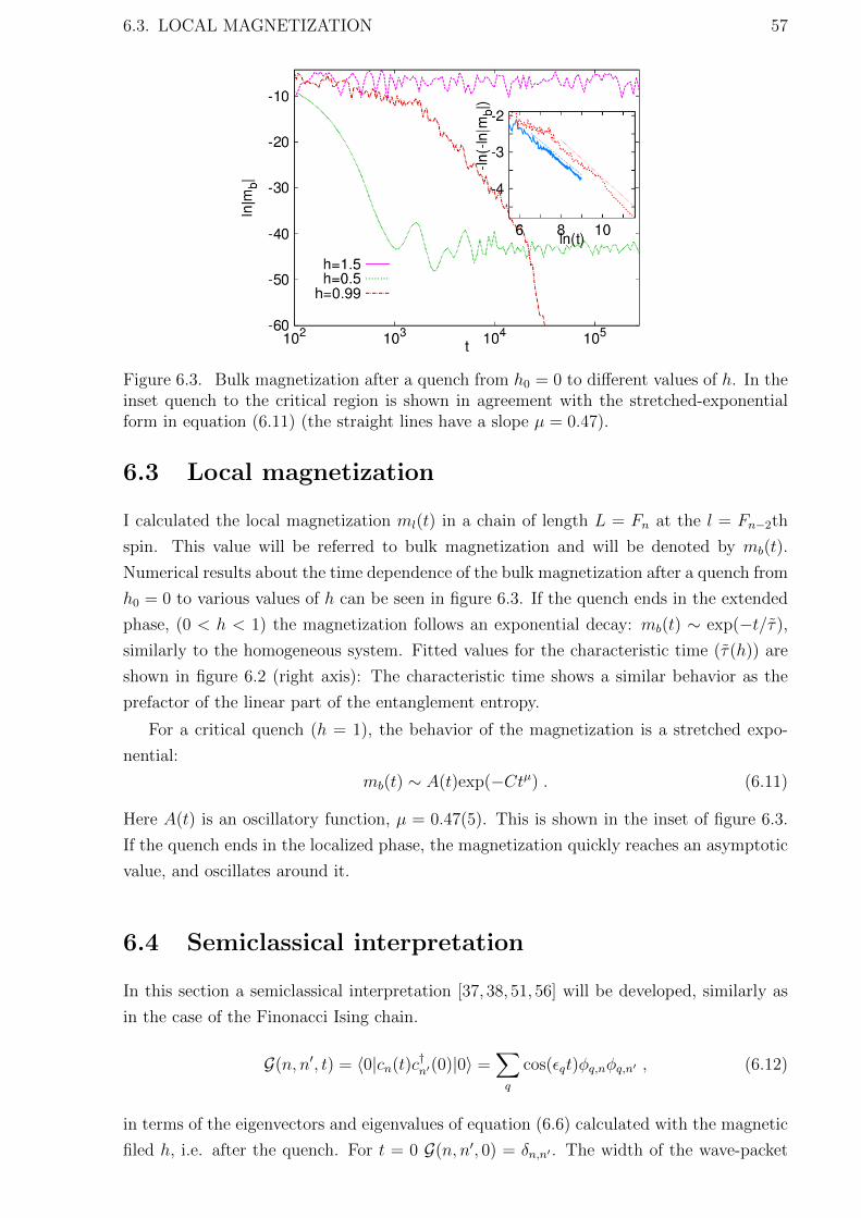
6.3. LOCAL MAGNETIZATION 57
Figure 6.3. Bulk magnetization after a quench from h0 = 0 to different values of h. In theinset quench to the critical region is shown in agreement with the stretched-exponentialform in equation (6.11) (the straight lines have a slope µ = 0.47).
6.3 Local magnetization
I calculated the local magnetization ml(t) in a chain of length L = Fn at the l = Fn−2th
spin. This value will be referred to bulk magnetization and will be denoted by mb(t).
Numerical results about the time dependence of the bulk magnetization after a quench from
h0 = 0 to various values of h can be seen in figure 6.3. If the quench ends in the extended
phase, (0 < h < 1) the magnetization follows an exponential decay: mb(t) ∼ exp(−t/τ),
similarly to the homogeneous system. Fitted values for the characteristic time (τ(h)) are
shown in figure 6.2 (right axis): The characteristic time shows a similar behavior as the
prefactor of the linear part of the entanglement entropy.
For a critical quench (h = 1), the behavior of the magnetization is a stretched expo-
nential:
mb(t) ∼ A(t)exp(−Ctµ) . (6.11)
Here A(t) is an oscillatory function, µ = 0.47(5). This is shown in the inset of figure 6.3.
If the quench ends in the localized phase, the magnetization quickly reaches an asymptotic
value, and oscillates around it.
6.4 Semiclassical interpretation
In this section a semiclassical interpretation [37, 38, 51, 56] will be developed, similarly as
in the case of the Finonacci Ising chain.
G(n, n′, t) = 〈0|cn(t)c†n′(0)|0〉 =∑q
cos(εqt)φq,nφq,n′ , (6.12)
in terms of the eigenvectors and eigenvalues of equation (6.6) calculated with the magnetic
filed h, i.e. after the quench. For t = 0 G(n, n′, 0) = δn,n′ . The width of the wave-packet

58 6. CHAPTER. QUENCH DYNAMICS OF THE HARPER MODEL
Figure 6.4. Time-dependent width of the wave packet at different amplitudes of thetransverse field.
started from site n after time t is given by (similarly to equation (5.8)):
d(n, t) =
[∑n′
(n− n′)2|G(n, n′, t)|2]1/2
, (6.13)
which is then averaged over the starting positions, thus d(t) = d(n, t).
The d(t) width has been calculated for various after quench transverse field, these results
can be seen in figure 6.4. In the extended phase, in agreement with previous results [102]
the wave packet width d(t) grows linearly, which can be interpreted as the quasi-particles
moving ballistically, i.e. with constant velocity. From this it follows, as in the homogeneous
chains [38], that the entanglement entropy grows linearly, and the magnetization decreases
exponentially.
If the quench ends in the localized phase (h > 1), the wave packet width d(t) remains
finite d(t) → d. We found, that this finite asymptotic value (d) is proportional to the
equilibrium localization length d ∼ ξ, see in the right panel of figure 6.1.
If the quench ends at the critical point h = 1, the width of the wave packet grows with
a power function of the time: d(t) ∼ tD, where D is D = 0.477(10) in correspondence with
the results of [102]. The anomalous diffusion of the quasi-particles lead to the power-law
increase of the dynamical entanglement entropy eq. (6.7), and the stretched exponential
behavior of the bulk magnetization equation (6.11). The semiclassical picture predict, that
the diffusion exponent of the wave packet D, the exponent of the entanglement entropy σ,
and the exponent of the magnetization µ should be equal, and indeed these tree are equal
within the errors of the numerical data.

6.5. DISCUSSION 59
6.5 Discussion
In this chapter we studied the quench dynamics of the Harper model.
If the quench ends in the localized phase, the entanglement entropy grows proportional
to the time, the magnetization decreases exponentially, and the diffusion exponent of the
wave packet is close to one. The dynamics is similar to the after quench dynamics of the
homogeneous systems: The reason is that the spectrum of the Harper model is absolutely
continuous in the extended phase.
If the quench ended in the localized phase, the width of the wave packet remains finite for
long times, similarly the entanglement entropy and the magnetization also reaches a finite
limiting value. The asymptotic value of the wave packet width is proportional with the
localization length d ∼ ξ = 1lnh
. For the asymptotic value of the entanglement entropy the
S ∼ | ln(h)|−σ′ relation was found with σ′ = 0.5(4).
If the quench ended at the critical point, power-law growth of the wave packet was found
d(t) ∼ t0.477 in agreement with the results of [102]. The entanglement entropy grows with
a power function of the time S(t) ∼ tσ with exponent σ ≈ 0.43(5). The local magnetiz-
ation decrease with a stretched exponential function: mb(t) ∼ exp(−Ctµ) with µ ≈ 0.47(5).
This chapter is based on the following article:
G. Roosz., U. Divakaran, H. Rieger, F. Igloi Non-equilibrium quantum relaxation across a
localization-delocalization transition Phys. Rev. B 90, 184202 (2014)
The numerical simulations presented in this chapter, and the quasi-classical reasoning
were done by me. The scaling about the entanglement is common work with Prof. Dr.
Heiko Rieger and Prof. Dr. Ferenc Igloi.

Chapter 7
Nearly adiabatic dynamics of the
Harper model
Here the term ”nearly adiabatic“ means that a parameter of the system is varied very
slowly. If the external parameter is varied infinitely slowly, the eigenstates of the initial
Hamiltonian evolve to the eigenstates of the final Hamiltonian.
If the system crosses during the above mentioned process a second order phase transition,
the dynamics slows down (the relaxation time diverges), and the system cannot follow the
variation of the outer parameter, regardless of how slow the variation is. In consequence
defects are generated. The standard ”paradigm” to describe the generation of the defects
is the so called Kibble-Zurek scaling.
7.1 Kibble-Zurek scaling
The Kibble-Zurek scaling gives a prediction about the density of the defects, using the
critical exponents of the (crossed) transition point. The scaling is first used by Tom W. B.
Kibble who studied the structure of the early universe [58]. Later it was applied to solid
state physics by Wojciech H. Zurek [59]. Let us denote the correlation length as ξ and the
correlation time as ξt, which are related as ξt ∼ ξz, where z is the dynamical exponent.
Let us suppose, there is a well defined moment, when the time evolution becomes non-
adiabatic. Time evolution become non-adiabatic when the variation of the instantaneous
relaxation time is faster than the typical speed of relaxation:
(change of ξt during ξt time) ∼ ξt . (7.1)
Which is equivalent with:
ξtξt ∼ ξt ⇒ ξt ≈ 1 (7.2)
Let’s denote the external parameter with δ. The critical point is δ = 0. The outer
parameter is varied linearly in time: δ(t) = (t − tcrit.)/τ . Here τ is a time scale, which
characterizes the speed of the process. The nearly adiabatic (very slow) limit is: τ 1.
The tcrit. time is the time when the system crosses the critical point. Of course, it is
basically possible to choose tcrit. to be the zero of the time scale, however in the later part
60

7.1. KIBBLE-ZUREK SCALING 61
of this chapter another choice will be appropriate.
Using the critical scaling of the correlation length ξ and relaxation time ξt one gets:
ξt ∼ ξz ∼ δ(t)−νz ∼ (|t− tcrit.|/τ)−νz (7.3)
Using the above relationship equation (7.1) takes the form:
1 ≈ ξt|t=t ∼|t− tcrit.|−(νz+1)
τ−νz. (7.4)
Here t is the time when the system loses the adiabatic behavior. The |t − tcrit.| time
difference is usually referenced in the literature as Kibble-Zurek time. One can calculate
the instantaneous localization length at time t = t:
|t− tcrit.| ∼ τνzνz+1 =⇒ ξ ∼ |t− tcrit.|1/z ∼ τ
ννz+1 . (7.5)
In the Kibble-Zurek scaling the instantaneous localization length at time t = t is con-
sidered to be the average distance of two defects, and the excitation probability P (τ) is
supposed to be proportional to the density of the defects:
P (τ) ∼ (density of deffects) ∼ 1
ξd∼ τ−
dν1+νz .
ξ~
- t~t
ξ
tcrit
Figure 7.1. The red curve represent the diverging relaxation time. One supposes, that thereis a given moment, when the time evolution becomes non-adiabatic. The time differencebetween the aforementioned moment and the crossing of the critical point is the so calledKibble-Zurek time.
Later (after we defined the excitation probability in our calculation) we return to the
Kibble-Zurek scaling, and investigate in details what is the Kibble-Zurek prediction for the
Harper model.

62 7. CHAPTER. NEARLY ADIABATIC DYNAMICS OF THE HARPER MODEL
7.2 Density of defects in the adiabatic dynamics
The transverse field is varied linearly (and slowly) h = h(t) = t/τ , and the defects created
during this process. I investigate the density of the created defects, as a function of the τ
time. The time evolution starts at t = −∞, when the absolute value of the magnetic field
is very large, h→ −∞, so the initial state is a classical product state. In the initial state
the direction of the magnetic field gives the direction of the spins: σzn = 1 (c†ncn = 1) for
cos(2πβn) > 0 and σzn = −1 (c†ncn = 0) for cos(2πβn) < 0.
I used chains of even lengths, so in the initial state half of the spins directed in −zdirection and half of the spins directed in +z direction, in fermionic language, the initial
state is half-filled. The time evolution of the system is driven by the time dependent
Schrodinger equation dΨ/dt = −iH(t)Ψ(t), with the initial condition Ψ(−∞) = Ψ0(−∞).
The ground state of the H(t) Hamiltonian operator at time t is Ψ0(t): This ground state
usually differs from the Ψ(t) state which latter one is the result of a non-equilibrium time
evolution. We will investigate how far the two states Ψ(t) and Ψ0(t) are from each other,
and what is the connection between the difference, and the ”speed” of the variation of the
magnetic field τ . To investigate such questions one has to quantify the difference of the
two states. To do this, we will define the total excitation probability P , with the use of
the fermionic representation.
The Heisenberg equation of motion of the cn,H(t) are linear (see in Appendix A.4 and [61]),
because the Hamiltonian in equation(6.3) is quadratic. The evolution of vectors φq,n(t)
satisfy the differential equation:
idφq,n
dt=
1
2φq,n−1 + hnφq,n +
1
2φq,n+1 , (7.6)
with the initial condition: φq,n(−∞) = φq,n(−∞), where the latter are given in equation
(2.39).
The vector φq,n(t) at t time is generally different from the vector φq,n(t) which corres-
ponds to the ground state of the H(t) instantaneous Hamilton operator. .
In the initial state at t = −∞ half of the fermionic states are occupied, these are
denoted by Q−. The other half of fermionic states, denoted by Q+, are empty. If the time
evolution would be perfectly adiabatic, all empty states would remain empty. We define
the excitation probability as:
Pt =2
L
∑q∈Q+
∑q′∈Q−
pq,q′ , (7.7)
where pq,q′ is called partial excitation probability and defined as:
pq,q′ =
∣∣∣∣∣∑n
φq,n(t)φq′,n(t)
∣∣∣∣∣2
. (7.8)
The excitation probability measures how many empty states become excited due to the
finite speed of the variation of the magnetic field. Pt is normalized: 0 ≤ Pt ≤ 1. If the

7.3. NUMERICAL RESULTS AND SCALING THEORY 63
dynamics would be perfectly adiabatic, the Pt excitation probability would remain zero.
For a process with finite speed τ , one waits that the slover process (larger τ) implies the
smaller excitation probability Pt.
localized extended localized
t
h(t)
ξ
Figure 7.2. Magnetic field h(t), and the instantaneous correlation length ξ(t) as a functionof the time during the quench. In the numerical calculations two type of quench protocolswere used: each of the start at t = −∞, the endpoints are t = 0 and t = +∞.
We investigated two kinds of final states: i) the quench ends at t = 0, in the middle
of the extended phase and ii) t = ∞, when the quench cross the full extended phase,
and goes to the localized phase on the other site. (With positive h.) In the first case the
localization-delocalization transition is crossed once (at h = −1), in the second case, the
localization-delocalization transition is crossed twice: first at h = −1, and at h = +1.
7.3 Numerical results and scaling theory
I investigated the adiabatic dynamics by numerical calculations. The time evolution was
calculated using a Runge-Kutta method with adaptive step size in time, to keep the relative
error less than 10−6. I used h = ±10 to approximate h → ±∞, and I tested that the
numerical results are stable, and do not change if I used h = ±20.
Numerical results of the excitation probability as a function of the time-scale τ can be
seen in figure 7.3. The excitation probability shows a power-law dependence in both cases:
Pt(τ) ∼ At(τ)τ−κ , (7.9)
but the prefactors, At(τ) have different functional forms.
When the quench ends at t = 0, and the localization-delocalization transition is crossed
only once, the prefactor shows log-periodic oscillations: A0(τ) ∼ sin2(log(τ/τ0)). This
type of log-periodic oscillations are common in quasi-periodic systems [177]. Due to the
oscillations, the exponent can be determined with some uncertainty:
κ = 0.45(5) . (7.10)

64 7. CHAPTER. NEARLY ADIABATIC DYNAMICS OF THE HARPER MODEL
Figure 7.3. Excitation probability as a function of the time-scale, τ , after an adiabaticprocess from h = −∞ to h = 0 (upper panel) and to h = ∞ (lower panel) calculated infinite systems of sizes L = 2Fn with n = 13, 14, . . . , 18.
If the localization-delocalization transition is crossed twice (at h = −1 and h = 1)
the prefactor has fast oscillations in τ : A∞(τ) ∼ sin2(τ/τ∞ + cst.) with τ∞ ≈ 0.15, and
a slower log-periodic oscillation is also present. The fast oscillations are analogous to the
Stuckelberg oscillations [178,179]. It is hard to obtain the exponent of the second protocol,
due to the fast oscillations, however the numerical data is compatible with the estimate
for κ in equation (7.10).
Now we will build a scaling picture to interpret the measured κ = 0.45 value.
First the traditional Kibble-Zurek scaling ( described in section 7.1) is used for the
Aubry-Andre model. In the Aubry-Andre model d = 1 and ν = z = 1 so the prediction
of the Kibble-Zurek scaling theory is κsc = 0.5, which is close to the numerical estimate,
but sightly different. The rigorous derivations of the Kibble-Zurek scaling assume trans-
lational invariance, so the Kibble-Zurek prediction is not guaranteed to be precise for an
inhomogeneous system. Here a scaling is developed specially for the Aubry-Andre model.
The concept of the Kibble-Zurek time scale tKZ = |t − tcrit| (7.5) is used, however, the
tKZ time scale is connected with a more special way to the excitation probability than in
the usual Kibble-Zurek scaling. The elementary transition probabilities pq,q′ , calculated at
t = 0 (for the first protocol) will be investigated. The pq,q′-s are arranged in decreasing
order, then the first (biggest) N is summed up:
P (N,L, τ) =2
L
N ′∑q∈Q+q′∈Q−
pq,q′ . (7.11)
This quantity is called partial excitation probability. (The prime on the sum denotes
that the summation involves not all terms, just the N largest.)
I calculated the fraction of the partial excitation probability, and the full excitation
probability P (N,L, τ)/P0(τ), for several system sizes and decay parameters (τ -s). For
large systems the P (N,L, τ) is a function of N/L2
P (N,L, τ) = π(N/L2)P0(τ) , (7.12)
for large enough τ .
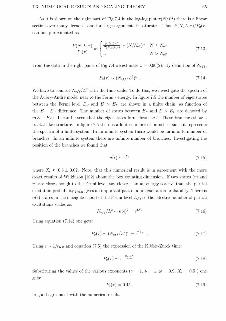
7.3. NUMERICAL RESULTS AND SCALING THEORY 65
As it is shown on the right part of Fig.7.4 in the log-log plot π(N/L2) there is a linear
section over many decades, and for large arguments it saturates. Thus P (N,L, τ)/P0(τ)
can be approximated as
P (N,L, τ)
P0(τ)≈
P (N,L,τ)P (Neff ,L,τ)
∼ (N/Neff)ω N ≤ Neff
1, N > Neff
(7.13)
From the data in the right panel of Fig.7.4 we estimate ω = 0.90(2). By definition of Neff :
P0(τ) ∼ (Neff/L2)ω . (7.14)
We have to connect Neff/L2 with the time scale. To do this, we investigate the spectra of
the Aubry-Andre model near to the Fermi - energy. In figure 7.5 the number of eigenstates
between the Fermi level EF and E > EF are shown in a finite chain, as function of
the E − EF difference. The number of states between EF and E > EF are denoted by
n(E − EF ). It can be seen that the eigenstates form ’branches’. These branches show a
fractal-like structure. In figure 7.5 there is a finite number of branches, since it represents
the spectra of a finite system. In an infinite system there would be an infinite number of
branches. In an infinite system there are infinite number of branches. Investigating the
position of the branches we found that
n(ε) ∼ εXe (7.15)
where Xe ≈ 0.5 ± 0.02. Note, that this numerical result is in agreement with the more
exact results of Wilkinson [102] about the box counting dimension. If two states (m and
n) are close enough to the Fermi level, say closer than an energy scale ε, than the partial
excitation probability pm,n gives an important part of a full excitation probability. There is
n(ε) states in the ε neighborhood of the Fermi level EF , so the effective number of partial
excitations scales as:
Neff/L2 ∼ n(ε)2 = ε2Xe (7.16)
Using equation (7.14) one gets:
P0(τ) ∼ (Neff/L2)ω = ε2Xeω . (7.17)
Using ε ∼ 1/tKZ and equation (7.5) the expression of the Kibble-Zurek time:
P0(τ) ∼ τ−2ωνzXeνz+1 (7.18)
Substituting the values of the various exponents (z = 1, ν = 1, ω = 0.9, Xe = 0.5 ) one
gets:
P0(τ) ≈ 0.45 , (7.19)
in good agreement with the numerical result.

66 7. CHAPTER. NEARLY ADIABATIC DYNAMICS OF THE HARPER MODEL
Figure 7.4. Normalized partial excitation probabilities as a function of (N/L)2 for differentsizes: L = 2Fn with n = 13, 14, . . . , 18 at τ = 100 (upper panel) the same at L = 2F18 fordifferent values of τ (lower panel) both in log-log scale.
1
10
100
1000
10000
1e-06 0.0001 0.01 1
log(
n)
log(E-EFermi)
Figure 7.5. Number of eigenstates between the Fermi energy (EF ) and E > EF , asa function of the E − EF difference. There are logarithmic scales of both axis. Theeigenstates are result of numerical calculation in a chain of length L = 2× 6765.
7.4 Discussion
In this chapter we studied a nearly adiabatic process in the Harper model. The amplitude
of the magnetic field h(t) was varied linearly in time with a rate 1/τ and studied the
density of defects in the ground state created during this process. If the localization-
delocalization transition point is passed once the density of defects follows a power-law
dependence, ∼ τ−κ, while if two symmetrically placed transition points are passed then
the density of defects has a multiplicative oscillating correction, similar to the Stuckelberg
phase of periodically driven two-level systems. Using scaling arguments we have related κ
to another critical exponents as given in equation(7.18). In this expression also the scaling
dimension ω of the excitation probability enters. For homogeneous systems it is generally
expected that ω = 1. In our case, when the spectrum of the Hamiltonian is not continuous
at the transition point, as well as the spectrum of the critical Hamiltonian is singular
continuous we have ω < 1. It is expected that ω 6= 1 is a general rule for quasi-periodic
and aperiodic Hamiltonians.
Finally, we discuss the question of the non-equilibrium dynamics of the Hamiltonian in
equation (2.17) for different values of the quasi-periodicity parameter β in equation (6.2).
If β is a rational number of the form β = 1/(2q) with q being an integer, then in the

7.4. DISCUSSION 67
adiabatic process the decay exponent is given by [74] κ = q/(q+ 1). The same result holds
for β = p/(2q), when p is an odd integer and p and q are relative primes, at least for not
too large values of q. Thus these results cannot be analytically continued to the case, when
β is an irrational number. If β is an irrational number and different from the inverse of the
golden mean ratio studied in this paper, than the critical exponents of the non-equilibrium
dynamics are expected to be β dependent. Some hint in favor of this assumption can
be found in the diffusion properties of the quasi-particles, see in section 6.4. Indeed the
diffusion exponent, D, is measured to be β dependent [102] and the same is expected to
hold for the non-equilibrium exponents σ and µ.
This chapter is based on the following article:
G. Roosz., U. Divakaran, H. Rieger, F. Igloi Non-equilibrium quantum relaxation across a
localization-delocalization transition Phys. Rev. B 90, 184202 (2014)
The numerical simulations presented in this chapter was done by me. Dr. Uma Divakaran
did stability investigations about the numerical method. The modified scaling theory
represented in the above chapter is also my work.

Chapter 8
Quench dynamics of the disordered
Ising model
8.1 Introduction
In this chapter we investigate the dynamics of the magnetization of the disordered trans-
verse field quantum Ising chain after a global quench. Concerning the functional form of
the relaxation process after a quench in random quantum systems, there have been de-
tailed studies about the time-dependence of the entanglement entropy [78–81, 180]. If the
system consists of non-interacting fermions - such as the random XX-spin chain or the
critical random transverse-field Ising chain - the dynamical entanglement entropy grows
ultra slowly in time as
S(t) ∼ a ln ln t , (8.1)
and saturates in a finite system at a value
S(`) ∼ b ln ` , (8.2)
where ` denotes the size of a block in a bipartite system and can be chosen to be pro-
portional to the size of the system L [79, 180]. These scaling forms can be explained by
a strong disorder renormalization-group (SDRG) approach [103]. Recently, the SDRG
method, which was designed as a ground state approach, has been generalized to take
into account excited states [181–183]; this generalized RG method is often abbreviated
as RSRG-X [181]. By this generalized SDRG method the ratio of the prefactors in (8.1)
and (8.2) is predicted as b/a = ψne, where ψne = 1/2 is a critical exponent in the non-
equilibrium process and describes the relation between time-scale and length-scale as
ln t ∼ Lψne . (8.3)
For interacting fermion models due to many-body localization the time-dependence of the
dynamical entropy is S(t) ∼ lnω t with ω ≥ 1, while the saturation value follows the volume
law, S(`) ∼ ` [81].
We consider relaxation processes from an initial ferromagnetic state and from a fully
68

8.2. THE MODEL 69
paramagnetic state by a sudden change of the strength of the transverse field. To cir-
cumvent numerical instability as observed in previous calculations for large systems using
eigenvalue solver routines [79,180], we use multiple precision arithmetic to study the time-
evolution through direct matrix multiplications.
8.2 The model
The model was introduced in Section 2.4, and the properties of the model also summarized
there. The model we consider is the quantum Ising chain of length L defined by the
Hamiltonian:
H = −1
2
L−1∑i=1
Jiσxi σ
xi+1 −
1
2
L∑i=1
hiσzi , (8.4)
in terms of the Pauli matrices σx,zi at site i. In this Chapter I will take free boundary
conditions. The homogeneous model with the uniform coupling Ji = 1 and the uniform
transverse field, hi = h, is in the disordered (ordered) phase for h > 1 (h < 1), and the
quantum critical point is located at h = 1. [111] The critical point of the model is described
by a conformal field theory with a central charge c = 1/2. In the random model with
quenched disorder, the Ji and the hi are position dependent, and are independent random
numbers taken from uniform distributions in the intervals [0, 1] and [0, h], respectively.
The random model is in the disordered (ordered) phase for h > 1 (h < 1) and the random
quantum critical point is at h = 1.
The free fermion representation of the Hamiltonian is:
H = −L∑i=1
hi(c†ici −
1
2)− 1
2
L−1∑i=1
Ji(c†i − ci)(c†i+1 + ci+1) , (8.5)
which is a special case of equation (2.2). The usual description of the dynamics is to
transform (8.5) to diagonal form, as it can be read in Appendix A, and as it was done in
the previous chapters. This method was applied to the disordered Ising chain, and it was
found that the eigenvalue solver routine fails to converge for some samples. The root of
the problem is that nearly degenerate eigenstates occur in some samples. The difference
between the energy levels of the states is comparable with the used numerical precision.
This causes that the eigenvalue solver routine returns false eigenstates. These events cause a
significant numerical error. To avoid instabilities, we follow a sightly difference procedure,
where only matrix products are used, and the rounding errors are controlled by using
multiple precision arithmetic.
8.2.1 Numerical calculation of time evolution
The Hamiltonian can be written in terms of Majorana operators:
H =1
4
2L∑n=1
2L∑m=1
am[Tm,n(i)(n−m)mod(2)
]an , (8.6)

70 8. CHAPTER. QUENCH DYNAMICS OF THE DISORDERED ISING MODEL
where
a2l−1 =L∑k=1
Φk(l)(η†k + ηk) ,
a2l = −ıL∑k=1
Ψk(l)(η†k − ηk) , (8.7)
are the Majorana operators. Some basic properties of these operators are included in
Appendix A.5. The T matrix is given as:
T =
0 h1
h1 0 J1
J1 0 h2
h2 0. . .
. . . . . . hL
hL 0
(8.8)
Using the canonical anti-commutators, one can derive the Heisenberg equation of mo-
tion of the Majoranna operators:
dan(t)
dt=
2L∑m=1
Mn,mam(t) . (8.9)
here M is a 2L×2L real matrix. In the upper triangle the elements of M and T are equal,
in the lower triangle the elements of T and M are opposite of each other.
M =
0 h1
−h1 0 J1
−J1 0 h2
−h2 0. . .
. . . . . . hL
−hL 0
(8.10)
One can expand the time dependent Majorana operators in the bases of the initial
Majorana operators as follows:
am(t) =2L∑n=1
Pmn(t)an(0) . (8.11)
Pmn(0) = δmn (8.12)
One obtains the following equations for the time evolution of the Pmn(t) coefficients:
dPn,k(t)
dt=
2L∑m=1
Tn,m(−1)n−mPm,k(t) =2L∑m=1
Mn,mPm,k(t) , (8.13)

8.2. THE MODEL 71
which can be written with short-hand matrix notation:
dP (t)
dt= MP (t) , (8.14)
with the initial condition Pn,m(0) = δn,m. The solution is P (t) = exp(Mt). It is possible
to evaluate the exponential using the eigenvalue decomposition of M , however there are
realizations where the eigenvalue solver routines fail to converge. To avoid the convergence
problems we evaluate the exponential for a unit time step tstep = 1 using the Taylor series
exp(Mtstep) =∑∞
n=0Mn
n!tnstep. In the numerical calculations, we used multiple precision
arithmetic to evaluate the Taylor-expansion, and summed the first 100 term in the expan-
sion. The first 100 term is enough to make the truncation error smaller than the used
numerical precision. The absolute value of the eigenvalues of M are smaller than 2 [120],
so the nth term is the Taylor expansion is smaller than 2ntnstep/n! in operator norm. The
time evolution is then calculated with matrix products,
P (2ntstep) = P (2n−1tstep)P (2n−1tstep) . (8.15)
I used two kinda of initial states, one ferromagnetic (h0 → 0+) state and one paramag-
netic (h0 → +∞) state.
In the ferromagnetic state Ψ(0)(k)j = δj,(k+1)mod(L) and Φ(0)(k)j = −δk,j. One gets for the
initial correlation matrix G(0)m,n = −∑L
k=1 Ψ(0)(k)mΦ(0)(k)j = δm,(n+1)mod(L).
In the paramagnetic state Ψ(0)(k)j = δj,k and Φ(0)(k)j = −δk,j, and one gets for the initial
correlation matrix G(0)m,n = δm,n.

72 8. CHAPTER. QUENCH DYNAMICS OF THE DISORDERED ISING MODEL
8.3 From fully ordered initial state to the ferromag-
netic phase
The fully ordered state is defined by h→ 0+. We investigated various after quench magnetic
field h = 0.5 . . . 0.9, and different lengths of the chain L = 16 . . . 128. The numerical results
are shown in figure 8.1. Let us first investigate the (a) panel of Figure 8.1. The bulk
-0.5
-0.25
0 1 2 3 4 5
log([
m(t
)]av)
log(log(t))
h=0.5
(a)
-0.5
-0.25
0 1 2 3 4 5
log([
m(t
)]av)
log(log(t))
h=0.6
(b)
-0.75
-0.5
-0.25
0 1 2 3 4 5
log([
m(t
)]av)
log(log(t))
h=0.7
(c)
-1
-0.75
-0.5
0 1 2 3 4 5
log([
m(t
)]av)
log(log(t))
h=0.8
(c)(d)
-1
-0.75
-0.5
0 1 2 3 4 5
log([
m(t
)]av)
log(log(t))
h=0.9
(e)
-1
-0.75
-0.5
0 1 2 3 4 5
log([
m(t
)]av)
log(log(t))
h=1.0
L=16
L=32
L=64
L=128
(f)
Figure 8.1. Quenches from the fully ordered initial state h0 = 0, to the ferromagnetic phaseand the critical point. Each sub-figure corresponds to a different magnetic field. (See thelabels above the sub-figures.) The different colors denote the different chain lengths. Thequench shown in the right bottom sub-figure ends in the critical point (h = 1), the othersends in the ferromagnetic phase (h < 1). The magnetization was calculated in the middleof the spin chain at site l = L/2.
magnetization decreases, first reach the first plateau, and after a system-size dependent
time, tp2 a fast decrease happens, and the magnetization reaches a second plateau. The
tp2 time goes to infinity in the thermodynamic limit: Therefore in the thermodynamic
limit the second plateau is absent. The end time of the first plateau scales in a finite
system as log(log tp2) ∼ logL, and the average magnetization in the second plateau scales
as log[mp2(L)/mp2(∞)] ∼ ξ/L, where ξ is the correlation length of the second plateau.
The other quenches ending in the ferromagnetic phase ( (b)-(e) panels in Figure 8.1) show
similar behavior. The end time of the first plateau tp2 become smaller and smaller as the
after quench magnetic field approaches the critical value 1, and if the quench ends in the

8.4. QUENCH TO THE CRITICAL POINT 73
critical point (Figure 8.1 (f) panel), there is no first plateau.
The double plateau behavior can be described in the framework of the semiclassical
theory. Quasi-particles are created at the time of the quench, and the magnetization on
a given site decrease, if a quasi-particle crosses the given site. In the ferromagnetic phase
of the disordered Ising chain, there is a finite correlation length ξ, and the quasi-particles
travels only ξ distance after the quench. When the quasi-particles traveled ξ distance from
the site of their creation, the decrease of the magnetization stops, and the first plateau is
created. If the after quench magnetic field h is closer to the critical point, the localization
length ξ becomes larger, and the average magnetization in the first plateau becomes smaller.
The second plateau and the second fast decrease of the magnetization are the results
of another, strictly finite-size effect. There is a special excitation in the ferromagnetic
phase, with exponentially small energy: ε0(L) ∼ exp(−L/ξ). The time scale where the
first decrease occur is tp2 ∼ 1/ε0, in correspondence with the numerical simulations. This
special excitation is also localized, and the average values of the second plateau goes to a
finite value in the thermodynamic (L→∞) limit. There is no such low energy excitation
in the critical point: There the lowest excitation is ε0(L) ∼ exp(−AL1/2).
8.4 Quench to the critical point
8.4.1 Ferromagnetic initial state
In Figure 8.2 the decay of the magnetization is shown after a quench from the ferromagnetic
initial state (h0 → 0+) to the critical point (h = 1). There is an asymptotic region where
log(m(t)) is proportional with log(log t), log(m(t)) ∼ a log(log t), where a ≈ 0.14.
m(t) ∼ (log(t))−a (8.16)
The asymptotic region ends after a finite size dependent time, ta(L). For the quasi-particles
emitted from the neighborhood of the boundaries, ta(L) amount of time is needed to reach
the investigated bulk spin at l = L/2. Before ta(L) the boundaries does not effect the
magnetization at site l = L/2, after ta(L) one observes finite-size effects in the dynamics
of the bulk magnetization. After this asymptotic region there is a short period of fast
decrease, and at the end there is the plateau region. For critical quenches there is only one
plateau region. The average magnetization of the plateau region (mp(L)) decreases with
the increasing system size (see Figure 8.3). The mp(L) average magnetization is a power
law of the system size (L)
mp(L) ∼ L−b , (8.17)
where b ≈ 0.068(5). Here the estimated error is the error of the numerical fit. The two
formulas (8.16) and (8.17) have to give the same result for t = ta(L), so one gets:
log ta(L) ∼ Lb/a whereb/a ≈ 0.489± 0.02 . (8.18)

74 8. CHAPTER. QUENCH DYNAMICS OF THE DISORDERED ISING MODEL
Comparing this result with the definition of the Ψ exponent:
Ψ = b/a . (8.19)
This agrees with the result of RSRG-X. The scaling described above is illustrated in the
right panel of Figure 8.2, where ln(Lbm(t)) is plotted against ln(ln t/LΨ).
The distributions of the variables in a disordered system are usually non-trivial, and often
contains important informations about the system.
We investigate the distribution of the log-magnetization in the plateau regime. The
probability distribution can be seen in Figure 8.3. The distribution is broad, and becomes
broader with larger system sizes. One gets a data collapse with the scaling variable y =
logmpL−α, thus
PL(logmp) = L−αp(logmpL−α), α = b = 0.0685 . (8.20)
as can be seen in Figure 8.3. The typical value of the magnetization in the plateau region
is exp(−ALα), which is much smaller than the average value, mp(L) ∼ L−b (see Equation
(8.17)). The contribution of the typical samples is very small, negligible in the thermody-
namic limit. The important contribution to the average of the magnetization comes from
the atypical samples, i.e. from the rare realizations. In those rare realizations the long
time limit of the magnetization is large mp(L) = O(1). The average of the magnetization
is given by the y → 0− behavior. It is assumed that for small values of y, p follows a power
law:
p(y) ∼ (−y)χ . (8.21)
The average of mp is given by:
[mp]av = L−α∫dmpp(logmpL
−α) (8.22)
∼ L−α∫dmp[logmpL
−α]χ ∼ L−α(1+χ) (8.23)
with α = b and χ = 0 (see figure 8.3) one gets [mp]av ∼ L−b, in agreement with the results
of the numerical calculations summarized in Equation (8.17).
8.4.2 Paramagnetic initial state
The fully paramagnetic initial state means, that the initial magnetic field is very large
h0 →∞, or equivalently all of the couplings vanish. In this state, all of the spins point to
the z direction, the magnetization is zero in the x direction, the initial correlation matrix
is diagonal: G(0)m,n = δm,n. I investigate quenches from the above described paramagnetic
state to the critical point h = 1. The time dependence of the average magnetization
are shown in Figure 8.4. The initial value is zero of the magnetization, which cannot be
represented on the logarithmic scale of equation (8.4). The magnetization decreases for
all global quenches in homogeneous or quasi-periodic chains. Surprisingly in the quench

8.4. QUENCH TO THE CRITICAL POINT 75
0 1 2 3 4 5ln(ln t)
-1.2
-1
-0.8
-0.6
lnm
L = 32L = 64L = 128L = 256
-3 -2 -1 0 1 2 3
ln(ln t / Lψ)
-0.8
-0.6
-0.4
-0.2
ln (
m L
b)
L = 32
L = 64
L = 128
L = 256
(b)
Figure 8.2. Left: Time evolution of the magnetization after a quench from h0 = 0.0 to thecritical point h = 1. The broken line denote a fit to the asymptotic region. Right Scalingplot of the relaxation of the magnetization after a quench from h0 = 0 to the critical pointin the disordered Ising chain the fitting parameters are b = 0.0685, Ψ = 0.5.
-12 -10 -8 -6 -4 -2 0ln(m)
10-3
10-2
10-1
P(ln
(m))
L = 32L = 64L = 128L = 256
-8 -6 -4 -2 0
ln(mp)L-b
10-4
10-3
10-2
10-1
P(l
n(m
p)
L-b
)
L = 32
L = 64
L = 128
L = 256
(b)
Figure 8.3. Left: Histogram of the plateau values after a quench from h0 = 0.0 to thecritical point. Right: Scaling plot of the histogram of the plateau values after a quenchfrom h0 = 0 to h1 = 1. Bottom: Average of the magnetization after a quench from h0 = 0to h = 1 in the plateau region.

76 8. CHAPTER. QUENCH DYNAMICS OF THE DISORDERED ISING MODEL
1 2 3 4 5
ln(ln t)
-40
-30
-20
-10ln
mL = 32
L = 64
L = 128
L = 256
101
102
103L
-8
-7
-6
-5
-4
ln(m
p)
(a)
-2 -1 0 1 2 3
ln(ln t/Lψ )
-30
-20
-10
0
ln(
m L
b' )
L = 32
L = 64
L = 128
L = 256
(b)
Figure 8.4. Panel (a): Time evolution of the order parameter after a quench from theparamagnetic state (h0 =∞), to the critical point h = 1 for different system sizes. In insetthe average asymptotic (plateau) values can be seen. Panel (b): Scaled plot of the timeevolution of the order parameter after a quench from the paramagnetic state (h0 =∞), tothe critical point h = 1 for different system sizes. The values of the scaling exponents areb′ = 1.46 Ψ = 0.5
investigated in this chapter the magnetization starts to increase and for long times reaches
an asymptotic plateau value. The average plateau values decay with the system size L,
and follow a power law:
[mp]av(L) ∼ L−b′, b′ = 1.4 . (8.24)
This behavior is shown in the inset of Figure 8.4. The dynamical magnetization shows
good scaling collapse, when mpLb′ is plotted against log t/LΨ, as it is shown in Figure 8.4 .
The large time limiting value of the dynamical magnetization, mp(L) was also studied, and
it is shown in Figure 8.5. It can be seen, that the logarithm of the magnetization is broadly
distributed. A good scaling collapse can reached with the scaling variable y = logmpL−α′ ,
with α′ = 0.5. The scaling is shown in Figure 8.5. It follows, that the typical values of
the magnetization scales with L as mtypp ∼ exp(−CLα), and it is much smaller than the
average. The average value is determined by rare events with contributions of O(1).
PL(logmp) = L−αp(logmpL−α′) . (8.25)
The average of mp(L) is determined by the behavior of the p(y) function on small negative
arguments. (The function p(y) is introduced in equation 8.25.) we assume that for small
y:
p(y) ∼ (−y)χ′. (8.26)
From figure 8.5 one can see χ′ = 2 and with similar reasoning as in equation (8.23) one
gets
[mp]av(L) ∼ L−α′(1+χ′) , (8.27)
in agreement with the numerical results.
With the investigation of the surface magnetization measured on the boundary site
(l = 1) of an open chain enables a better understanding of the scaling behavior of the

8.4. QUENCH TO THE CRITICAL POINT 77
-40 -30 -20 -10 0
ln(mp)
10-6
10-4
10-2
100
P(l
n(m
p))
L = 32
L = 64
L = 128
L = 256
-2 -1
y = ln(mp / L0.5 )10
-1
100
P(y
)
(a)
0.1 1
-y = ln(mp)/L0.5
10-2
100
P(-
y)
L = 32
L = 64
L = 128
L = 256
(b)
Figure 8.5. (a): Histogram of the plateau values after a quench from h0 =∞ to the criticalpoint. (b): Histogram of the plateau values after a quench from h0 = ∞ to the criticalpoint. The P (log(mL1/2)) - log(m)L1/2 scaling gives a good data collapse.
long-time limiting value of the dynamical order parameter. With the results of Ref. [176])
(see equation (16)) the long-time limiting value of the surface magnetization, msp, can be
calculated exactly:
msp = Φ1(1)
L∑j=1
Φ1(j)Φ(0)1 (j) . (8.28)
Here:
Φ1(j) = Φ1(1)
j−1∏i=1
hiJi,
Φ1(1) =
[1 +
L−1∑l=1
l∏j=1
(hjJj
)2]−1/2
. (8.29)
In the large-h0 limit for Φ(0)1 (j) one gets Φ
(0)1 (j) = δlm,j. Here lm is the position of the
largest transverse field in the sample [184]. Thus
msp = [Φ1(1)]2
lm−1∏j=1
(hjJj
), (8.30)
where Φ1(1) = mseq is the equilibrium value of the surface magnetization of the chain [117,
185], evaluated in the final state, i.e. with h = hc.
The typical value of mseq at the critical point scales as exp(−CL1/2) [117, 186]. The
same scaling combination holds for msp. As a consequence the right scaling combination
for msp is y = ln(ms
p)L−1/2. It is the same form that has been obtained for the bulk spins
above. From the scaling behavior of the average value msp it can be seen, that the rare
events are dominant.
The scaling of the surface magnetization can be calculated using an analogy with ran-
dom walks. There is a direct connection between the random transverse-field Ising chain
and a one-dimensional random walk ( [117]): to a given sample (given magnetic fields hi

78 8. CHAPTER. QUENCH DYNAMICS OF THE DISORDERED ISING MODEL
and couplings Ji for i = 1, 2, . . . L) a one-dimensional random walk is associated. The
associated random walk starts at the origin and takes consecutive steps, the length of the
i-th step being ln(hi/Ji).
The associated random walk stays at positive positions for all steps (In other words it
is a surviving walk.) for rare realizations of mseq. Concerning ms
p, here for a rare realization
both mseq and the product
∏lm−1j=1
(hjJj
)should be of order of O(1). In the random walk
language it means that the walk is surviving and returns after lm steps.
The probability of this particular event is: P(lm) ∼ l−3/2m (L − lm)−1/2. The average
value scales as:∑
lmP(lm)/L ∼ L−3/2, which means that ms
p(L) ∼ L−3/2. The scaling
behavior, extracted from the numerical data is similar to the last form.
8.5 Discussion
In this section we investigated numerically the dynamics of the local magnetization after a
quench in the transverse quantum Ising chain. In order to get precise numerical results we
avoided to use eigenvalue solver routines, since routine stability problems were reported in
the literature [122] [187]. I calculated the time evolution of Majorana operators using only
matrix products and multiple precision arithmetic.
If the quench starts from the ferromagnetic state and ends in the ferromagnetic phase the
magnetization first reaches a plateau value, and after a delay time a second relaxation
occurs, and the magnetization reaches a second plateau value. The second relaxation is
generated by quasi-localized modes which are present in the ferromagnetic phase of a finite
system. In an infinite system only the first plateau exists. The average magnetization is h
dependent and finite in both plateaus.
If the system is quenched from the ferromagnetic phase to the critical point the magnet-
ization goes to zero in an infinite system, as ml(t) ∼ (ln(t))−a. In a finite system the
magnetization reaches a finite L dependent limiting value. The distribution of the long-
time limiting value of the magnetization was investigated. The typical value goes to zero
starched exponentially with the system size (exp(−CLα)), but the average is dominated
by rare events, and decays with a power law of the system size.
If the quench start from the paramagnetic state and ends in the critical point a rapid
increase of the average magnetization was found, which is a unique property of the random
chain: After any quench in the homogeneous or quasi-periodic Ising chain the magnetiza-
tion decays.
This chapter is based on the following article:
G. Roosz., Y.-C. Lin, F. Igloi Critical quench dynamics of random quantum spin chains:
Ultra-slow relaxation from initial order and delayed ordering from initial disorder New J.
Phys. 19, 023055 (2017)
I did the numerical simulations presented in the above chapter, and the scaling analysis
about the bulk magnetization is also my own work. The analysis of the surface magnetiz-
ation was did by Prof. Dr. Ferenc Igloi.

Chapter 9
Conclusion
In this dissertation I investigated the dynamics of inhomogeneous one dimensional systems
with free-fermion techniques. Different types of inhomogeneities were investigated (local
defect, two types of quasi periodic modulation, and a disordered system). The main results
are the following:
1. For the generalized local defect I checked using large scale numerical simulations the
conjuncture about the dynamics of the local magnetization at the defect site. Here
the term generalized means, that a coupling and the two neighboring magnetic fields
differs from the critical value. The dynamics is function of the quench parameter κi
which is a combination of the coupling, and the magnetic fields: κi = Jih1ih2i
. Here
κ1 describes the pre-quench system, and κ2 describes the after quench system. The
time evolution of the magnetization in a finite system of length L is:
md(t, L)∼L−x1
[L sin
(πt
L
)]2(x12−x2)
, 0 < t < L .
where the exponents are xi =√
2π
arctan( 1κi
) and x12 =√x1x2. (i = 1, 2)
2. For the Fibonacci Ising chain I investigated the after dynamics of the local magnetiz-
ation numerically using free fermion methods. I found that the magnetization follows
a stretched exponential decrease:
mb(t) ∼ A(t)exp (−Ctµ) .
I also found a dynamical phase transition in the behavior of the magnetization: There
is a critical magnetic field h∗ if the after quench magnetic field is bigger than h∗, the
A(t) prefactor of the magnetization oscillates, if the after quench magnetic field is
below h∗ the prefactor A(t) remains positive. In a homogeneous system h∗ = 1, in
the Finonacci Ising chain h∗ < 1, and h∗ is power law of the inhomogeneity strength.
For the entanglement entropy and for the wave-packet power-law increase were found.
The exponents of the magnetization, entropy, and wave packet are close to each other
in the non-oscillatory phase. This phenomenon was understood using a quasi-classical
reasoning.
79

80 9. CHAPTER. CONCLUSION
3. I investigated the quench dynamics of the Harper model, which shows a localization-
delocalization phase transition. I calculated the after-quench dynamics of the en-
tanglement entropy and the local magnetization. If the quench ends in the localized
phase, the dynamics is similar to the dynamics of an homogeneous system: The en-
tanglement entropy grows linearly in time, the magnetization decrease exponentially,
the wave packet shows a ballistic spread. If the quench ends in the localized phase,
the entropy and the magnetization both remains finite in the long-time limit, and
the width of the wave packet remains small, comparable with the static localization
length.
If the quench ends at the critical point, the magnetization decreases with a stretched
exponential function mb(t) ∼ A(t)exp (−Ctµ), and the entropy grows with a power
function S ∼ tσ of the time. The spreading of the wave packet follows a power law
d(t) ∼ t0.477 [102]. The exponents µ and σ are close to the exponent of the wave-
packet spread. This fact has been understood based on a quasi-classical reasoning.
4. I investigated a Kibble-Zurek process in the Harper model. The defect density scales
with a power of the speed of the process P ∼ 1/τκ. The prediction of the standard
Kibble-Zurek scaling for the exponent is κ = 1/2. My numerical data suggest smaller
exponent, κ ≈ 0.45. I developed a modified version of the Kibble-Zurek scaling for
the Harper model. This modified scaling is in good agreement with the numerical
data.
5. I investigated the after quench dynamics of the magnetization in the disordered trans-
verse Ising model. I investigated three types of quenches: from a totally ferromagnetic
(h0 = 0) state to the ferromagnetic phase (0 < h < 1), from the totally ferromagnetic
phase (h0 = 0) to the critical point (h = 1), and from the totally paramagnetic state
(h0 →∞) to the critical point (h = 1).
If the quench starts from the totally ferromagnetic state, and ends at the critical
point, the magnetization remains constant in the long time limit.
If the quench starts from the infinitely paramagnetic phase and ends at the critical
point, the magnetization of the finite system increases, which is a unique fact of this
disordered system. If L → ∞, the asymptotic magnetization goes to zero in the
aforementioned quench.
If the quench starts from the totally ferromagnetic phase (h0 = 0) and ends at the
critical point, the magnetization shows an extremely slow decrease of the form:
m(t) ∼ (log(t))−a
where a ≈ 0.14.

10. fejezet
Osszefoglalo
10.1. Bevezetes
A zart kvantumrendszerek kulso parameterek megvaltoztatasat koveto dinamikaja aktıvan
kutatott terulet, mind kıserleti, mind elmeleti tekintetben. A parameter megvaltoztatasanak
sebessege szerint ket szelsoseges esetrol beszelhetunk. A kulso parameter hirtelen megvaltoztatasat
”kvencs”-nek nevezzuk. A valtoztatas utani dinamikat kvencs utani dinamikanak Kıserletileg
a kvencs utani dinamika a Feshbach rezonancia segıtsegevel valosıthato meg [1–11].
A kvencsekkel kapcsolatban az egyik kerdeskor az, hogy a fizikai mennyisegek hogyan
valtoznak roviddel a parameter megvaltoztatasa utan. A masik kerdeskor azt vizsgalja,
hogy a kvencs utan nagyon hosszu ido elteltevel milyen allandosult allapot alakul ki, mi a
kapcsolata a kialakult allandosult allapotnak a rendszerben letezo megmarado mennyisegekkel.
[12–57]. A masik hatareset a parameter nagyon lassu valtoztatasa, a kozel adiabati-
kus dinamika. A kulso parametert a legtobbszor idoben linearisan valtoztatjak ∼ t/τ
modon, es a valtoztatas soran atvisszuk a rendszert egy fazisatalakulasi ponton. A folya-
mat elejen a rendszer a pillanatnyi Hamilton-operator alapallapotaban van. Ha a parameter
valtoztatasanak sebessege (1/τ) sokkal kisebb mint a rendszerben talalhato legkisebb ener-
gia kulonbseghez tartozo idoskala, a rendszert jellemzo allapotvektor mindvegig kozel ma-
rad a pillanatnyi alapallapothoz. Azonban a legkisebb energia kulonbseg (legkisebb gap)
nullahoz tart, ahogy a rendszer kozelıt a fazisatalakulasi ponthoz, ıgy a kulso parameter
valtozasa nem lesz a folyamat egesz ideje alatt ”eleg lassu”.
A kerdes, hogy milyen messze lesz a lassu dinamikaval kapott allapot az alapallapottol a
fazisatalakulasi pont keresztezese utan, intenzıv vizsgalatok targyat kepezte [50,56,58–74].
Kibble es Zurek [58] [59] megadott egy osszefuggest, amely a ket allapot ”tavolsagat”
a P (τ) ∼ (density of deffects) ∼ 1ξd∼ τ−
dννz+1 modon jellemzi, ahol d a rendszer dina-
mikaja, ν a korrelacios hossz kritikus exponense, z a dinamikai exponens. A formula
eredeti indoklasa heurisztikus, azota perturbatıv es numerikus modszerekkel vizsgaltak az
ervenyesseget kulonbozo rendszerekben.
Az itt kiemelt ketfele folyamat mellett az irodalomban mas nemegyensulyi dinamikaval
kapcsolatos kerdeseket is vizsgaltak, ilyen peldaul egy izolalt rendszer idofejlodese idoben
periodikusan [75] [76], kvazi-periodikusan vagy veletlenszeruen [77] valtozo kulso poten-
cialban.
81

82 10. FEJEZET. OSSZEFOGLALO
A kvencs dinamikaval kapcsolatban kiterjedt irodalom letezik, amelyben azonban leginkabb
a homogen (transzlacio invarians) rendszerek dinamikajat vizsgaltak [12,16–33,50,51,55]. A
homogen rendszerekkel kapcsolatban az egyik legszebb eredmeny a kvencs utani dinamika
kvazi-klasszikus leırasa. A kvencs soran a rendszer minden pontjaban kvazireszecske parok
keletkeznek ellentetes impulzussal. Ezek a reszecskek a kesobbiek soran allando sebesseggel
haladnak, a rendszert hatarolo feluletekrol visszaverodnek [38, 51, 56]. A kvaziklasszikus
leıras segıtsegevel a homogen rendszerekre aszimptotikusan egzakt eredmenyek kaphatoak.
Az inhomogen rendszerek kvencs utani dinamikajaval kapcsolatban csak nehany specialis
esetet vizsgaltak az irodalomban, peldaul az osszefonodasi entropia viselkedeset rendezetlen
spinlancokban [78–80], vagy a soktest-lokalizacio modelljeiben [81] [82]. Az inhomogenitas
egy specialis tıpusa a kvazi-periodikus rend, ami a homogen es a rendezetlen rendszerek
”kozott” helyezkedik el: bonyolultabb az elobbinel, hisz nem transzlacio invarians, de egy-
szerubb az utobbinal, mert rendezett, determinisztikus [83–85].
A kvaziperiodikus rendszerek szokatlan transzporttulajdonsagokkal bırnak, bennuk a hullamcsomag
kiterjedese nem ”ballisztikus” mint a homogen rendszerekben, hanem anomalis diffuziot
kovet [86, 87].
A disszertacio az alabbi negy cikken alapul:
1. F. Igloi, G. Roosz, Y.-C. Lin Nonequilibrium quench dynamics in quantum quasicrys-
tals New J. Phys. 15, 023036 (2013)
2. F. Igloi, G. Roosz, L. Turban Evolution of the magnetization after a local quench in
the critical transverse-field Ising chain J. Stat. Mech. (2014) P03023
3. G. Roosz., U. Divakaran, H. Rieger, F. Igloi Non-equilibrium quantum relaxation
across a localization-delocalization transition Phys. Rev. B 90, 184202 (2014)
4. G. Roosz., Y.-C. Lin, F. Igloi Critical quench dynamics of random quantum spin
chains: Ultra-slow relaxation from initial order and delayed ordering from initial
disorder 2017 New J. Phys. https://doi.org/10.1088/1367-2630/aa60e6
A kovetkezo alfejezetekben a disszertacio sajat eredmenyeket ismerteto reszeinek magyar
nyelvu kivonata olvashato.
10.2. Altalanosıtott lokalis kvencs
Ebben a fejezetben az angol nyelvu szoveg 4 fejezetet foglalom ossze, amely a [188] cikken
alapul. Az irodalomban a legtobbet vizsgalt kerdeskor az un. globalis kvencs: Ekkor a
rendszer egy parametere globalisan, az egesz rendszerre kiterjedo homogen modon valtozik
meg: Ilyen peldaul egy kulso magneses ter bekapcsolasa, amelynek erteke az egesz rendszer
teruleten homogen. Egy masik erdekes kerdeskor a lokalis kvencsek terulete, amikor a Ha-
milton operator egy racshely kornyezeteben valtozik meg pillanatszeruen. Kıserletekben a
lokalis kvencset valosıt meg peldaul a rontgensugarak fembeli elnyelodese [141].
10.2. ALTALANOSITOTT LOKALIS KVENCS 83
Az elmeleti vizsgalatok tobbsege kritikus egydimenzios rendszerekkel foglalkozik, amelyek-
re vonatkozoan a konform terelmelet segıtsegevel egzakt eredmenyeket lehet megfogal-
mazni. A konform terelmelet a modell folytonos hataresetet ırja le, ahol a rendszer egy
ketdimenzios (x, t) teridoben el. Ebben a fejezetben egy kritikus transzverzalis teru kvan-
tum Ising lancot vizsgalunk, amelyben egy altalanosıtott hibahely parametereit pillanat-
szeruen megvaltoztatjuk. Az altalanosıtott jelzo arra vonatkozik, hogy egy csatolas es a
ket szomszedos magneses ter erteke is kulonbozik a kritikus lancra jellemzo tombi ertektol.
Az altalunk vizsgalt rendszer Hamilton-operatora:
Hi=−1
2
[L−1∑n=1
σxnσxn+1+(Ji−1)σxL/2σ
xL/2+1+
L∑n=1
σzn+(hi1−1)σzL/2 + (hi2−1)σzL/2+1
], (10.1)
ahol σxn, σyn, σzn a pauli matrixok. A hibahely a lanc kozepen talalhato, es a kvencs elott
(t < 0) J1 csatolas, attol balra h11 magneses ter, a J1 csatolastol jobbra h12 magneses
ter jellemzi. A kvencs utani parameterek J2, h21, h22. A kvencs utan a hibahelyen
mert lokalis magnesezettseg idobeli fejlodeset vizsgaljuk. A lokalis magnesezettseget a
σx operator alapallapot es elso gerjesztett allapot kozotti matrixelemekent szamıthatjuk
[167] mn(t)〈Φ0|σxn(t)|Φ1〉 egy tetszoleges racsponton. A magnesezettseg a hibahelyen:
md(t) = mn=L/2(t). A rendszer megfeleltetheto egy ketdimenzios klasszikus spin mo-
dell extrem-anizotrop esete transzfermatrixanak. A megfeleltetes segıtsegevel levezetheto
a lokalis magnesezettseg imaginarius idobeli dinamikaja a termodinamikai hataresetben
(L→∞ hataresetben). Az eredmenyek a kovetkezokepen foglalhatok ossze: A dinamika a
κi = Jihi1 hi2
(i = 1, 2) effektıv kolcsonhatasok fuggvenye, a magnesezettseg imaginarius
idobeli valtozasa hatvanyfuggvenyt kovet a
md(τ) ∼ τx12−x2 , 0 < τ L (10.2)
alakban, ahol az exponensek ertekei: xi =√
2π
arctan( 1κi
) es x12 =√x1x2. A valos ideju
dinamikara ismertek az irodalombol eredmenyek ha h11 = h12 = h21 = h22 = 1, es a
J1 = ∞ (a kezdeti allapotban a hibahely spinjei rogzıtettek) vagy J1 = 1 es J2 = 0 (egy
homogen lanc szetvagasa).
A rogzıtett spinu esetre [142] konform terelmelet segıtsegevel meghataroztak hogy a
magnesezettseg relaxacioja:
m(+)d (t) ∼ t−2xm 0 < t L . (10.3)
ami numerikus szimulaciokkal is tesztelve lett a transzverzalis teru kvantum Ising lancban
[94]. Egy nyılt lancban [94] eredmenyei a kovetkezo formulaval osszegezhetoek:
m(+)d (t, L) ∼
[L sin
(πt
L
)]−2xm
, 0 < t < L . (10.4)
Abban az esetben, amikor a ket felrendszer a kvencs utan nincs osszekapcsolva [94] nume-

84 10. FEJEZET. OSSZEFOGLALO
rikus eredmenyeit az alabbi formulaval lehet osszefoglalni:
m(fb)d (t, L) ∼ L−1/2
[L sin
(πt
L
)]1/4
, 0 < t < L . (10.5)
ami rovid idokre a kovetkezo alakot veszi fel:
m(fb)d (t) ∼ m0(L) t1/4, 0 ≤ t L , (10.6)
ahol m0(L) ∼ L−xms az egyensulyi erteke a hibahelyi magnesezettsegnek a kiindulasi
allapotban. Az exponens a (10.6) egyenletben megegyezik 1/4 = 2(xms/2 − xm) -vel,
ahol x2 = xm and x12 = xms/2. A rogzıtett spinu kezdoallapotra, (10.4) egyenlet, ugyanez
teljesul x12 = 0-el. Ha t2-et helyettesıtunk τ helyere az imaginarius idore vonatkozo egyen-
letekbe akkor a (10.2) egyenletbol megkaphatjuk a valos idore vonatkozo eredmenyeket, a
(10.4) es (10.6) egyenleteket. Ezert megfogalmazhatjuk a hibahelyi magnesezettseg kvencs
utani viselkedesere (az L 1 hataresetben) az alabbi sejtest:
md(t) ∼ m0(L) t2(x12−x2), 0 < t L , (10.7)
ahol m0(L) ∼ L−x1 . Egy veges rendszerben sejtesunk szerint a magnesezettseg a kovetkezo
(periodikus) modon valtozik a kvencs utan:
md(t, L)∼L−x1
[L sin
(πt
L
)]2(x12−x2)
, 0 < t < L . (10.8)
A fenti ket egyenlet a fejezet fo eredmenye. A sejteskent megfogalmazott formulakat nu-
merikus szimulacioval ellenoriztem.
10.3. A Finonacci Ising kvazikristaly nem egyensulyi
dinamikaja
Ebben a fejezetben a kvantum Ising lanc egy kvaziperiodikus valtozatanak dinamikajat
vizsgaljuk. A modellt definialo Hamilton-operator a kovetkezo:
H = −1
2
[∑i
Jiσxi σ
xi+1 + h
∑i
σzi
], (10.9)
( σxi , σzi a Pauli matrixok az i. helyen) A Ji csatolasok helyfuggoek, es az alabbi modon
vannak parameterezve:
Ji = Jrfi , (10.10)
itt r > 0 az inhomogenitas erosseget jellemzi, r = 1 megfelel a homogen rendszernek, minel
kisebb r annal erosebb az inhomogenitas. Az fi szamok 0 vagy 1 erteket vehetnek fel, es
kvaziperiodikusan valtakoznak az un. Fibonacci sorozatnak megfeleloen.

10.3. A FINONACCI ISING KVAZIKRISTALY NEM EGYENSULYI DINAMIKAJA 85
A J kolcsonhatas erosseg a (10.10) egyenletben J = r−ρ, ahol
ρ = limL→∞
∑Li=1 fiL
= 1− 1
ω, (10.11)
az 1 szamok aranya egy nagyon hosszu (vegtelen sorozatban).
A Fibonacci sorozatot a kovetkezo algebrai kifejezes definialja:
fi = 1 +
[i
ω
]−[i+ 1
ω
], (10.12)
ahol [x] az x szam egeszresze, es ω = (√
5 + 1)/2. A fenti definıcioval a modell kritikus
pontja h = 1-ben van, h < 1 a ferromagneses fazis, h > 1 a paramagneses fazis. A Fi-
bonacci sorozat a Harris-Luck kriterium szerint [204] irrelevans perturbacio: A kritikus
exponensek folytonosan valtoznak a rendezetlenseg erossegenek fuggvenyben.
A kvencset a magneses ter hirtelen valtoztatasaval valosıtottam meg. A kvencs elott a
magneses ter h0 a kvencs utan a magneses ter erteke h. Vizsgaltam a lokalis magnesezettseg
viselkedeset a hatarfeluletektol tavol, a tombi reszben, az osszefonodasi entropia idobeli
valtozasat, es az un. hullamcsomag kiszelesedeset. Az osszefonodasi entropia definıcioja a
kovetkezo. A rendszer a |Ψ〉 tiszta allapotban van, amit a ρ = |Ψ〉〈Ψ| diadikus surusegmatrixszal
is jellemezhetunk. A rendszert ket reszre osztjuk (A es B). Definialjuk a redukalt suruseg
matrixokat ρA = TrBρ es ρB = TrAρ. Az osszefonodasi entropia a redukalt surusegmatrixok
von Neumann entropiaja: S = −TrBρB ln ρB = −TrAρB ln ρA Az osszefonodasi entropia
a ket resz kozotti osszefonodast jellemzi. Numerikus szimulaciok segıtsegevel a kovetkezo
eredmenyekre jutottam: A magnesezettseg kvencs utani dinamikaja nyujtott exponencialis
viselkedest mutat:
mb(t) ∼ A(t)exp (−Ctµ) . (10.13)
az A(t) prefaktor egysegnyi nagysagrendu. Az A(t) prefaktor viselkedeseben ket tar-
tomanyt kulonıthetunk el h < h∗(r), akkor A(t) > 0 ha h < h∗(r) akkor A(t) oszcillal.
A h∗(r) dinamikai fazisatalakulasi pont az r parameternek hatvanyfuggvenye: h∗(r) ∼ rω
ahol ω ≈ 0.24 adodik. A h∗(r) ∼ rω osszefugges azzal a feltevessel all osszhangban,hogy
a magnesezettseg akkor marad pozitıv, ha a vizsgalt racshely kornyezete lokalisan fer-
romagneses, es akkor csokken oszcillalva, ha a kornyezet lokalisan paramagneses. Az ossze-
fonodasi entropia a kvencs utan az ido hatvanyfuggvenyekent no:
S(t) ∼ tσ , (10.14)
a σ exponens kozel megegyezik a magnesezettsegnel bevezetett µ exponenssel abban a
tartomanyban, ahol a magnesezettseg oszcillacio nelkul tart 0-hoz. Ezt a numerikus meg-
figyelest kvalitatıven a kvazi-klasszikus elmelettel ertelmeztem.

86 10. FEJEZET. OSSZEFOGLALO
10.4. A Harper-modell nem egyensulyi dinamikaja
A Harper-modellt definialo Hamilton-operator:
H = −1
4
L∑n=1
(σxnσxn+1 + σynσ
yn+1)−
L∑n=1
hnσzn . (10.15)
ahol σx,y,zn a Pauli-matrixok az n. racshelyen es hn egy kvaziperiodikus potencial:
hn = h cos(2πβn) , (10.16)
ahol β = (√
5−1)/2 az aranymetszes inverze. A Harper-modell lokalizacios fazisatalakulast
mutat [102], |h| < 1-re a modell sajat allapotai kiterjedtek, a spektrum abszolut folytonos,
|h| > 1-re a sajat allapotok lokalizaltak, a modell pontspektrummal bır. A kritikus pont-
ban (|h| = 1) a modell spektruma fraktal-szeru, szingularis-folytonos [113]. A kvenccsel
kapcsolatos numerikus eredmenyeket aszerint ırom le, hogy a kvencs utani h magneses ter
melyik fazisban van.
Ha a kvencs a kiterjedt fazisban vegzodott, a Harper-modell dinamikaja a homogen rend-
szerekere emlekeztet: A lokalis magnesezettseg exponencialisan csokken, az osszefonodasi
entropia az idovel linearisan no, a hullamcsomag ballisztikusan szelesedik. Ha a kvencs a
lokalizalt fazisban vegzodik, a lokalis magnesezettseg es az entropia is veges erteku marad.
Ha a kvencs a kritikus pontban vegzodik, a lokalis magnesezettseg nyujtott exponencialis
viselkedest mutat mb(t) ∼ A(t)exp (−Ctµ) ahol µ ≈ 0.43(5), az entropia S(t) ∼ tσ visel-
kedest mutat, ahol σ ≈ 0.47(5). Mind a σ mind a ν exponens kozel esik a [102] cikkeben a
hullamcsomag kiszelesedesere meghatarozott 0.477 ertekhez. Az exponensek kozeli erteke
arra enged kovetkeztetni, hogy a kvazi-klasszikus kep kvazi-periodikus rendszerek eseteben
is helyes, csupan a kvazi-reszecske parok homogen rendszerbeli ballisztikus mozgasat kell
a megfelelo anomalis diffuzioval helyettesıteni.
10.5. Kozel adiabatikus dinamika a Harper modellben
Ebben a fejezetben a Harper-modell kozel adiabatikus dinamikajaval kapcsolatos eredmenyeket
osszegzem. Az adiabatikus dinamikaval kapcsolatban ketfele ”protokollt” hasznaltam: Az
elso soran a h magneses ter erteke −∞-bol indul, es h = t/τ modon novekszik∞ ertekig. A
masodik protokoll soran a magneses ter szinten −∞-bol indul, es h = t/τ modon novekszik,
de csak h = 0-ig. Az elso protokoll soran a fazisatalakulasi pontot ketszer keresztezzuk, a
masodik protokoll soran egyszer.
A fazisatalakulasi pontokon valo athaladas soran a rendszerben gerjesztesek keletkeznek.
Annak valoszınusegere, hogy a rendszer gerjesztett allapotban lesz, a hagyomanyos Kibble-
Zurek skalazas P ∼ 1/τ 1/2-et josol [58]. A numerikus adataim P ∼ 1/τ 0.45-el kompatibili-
sek. A Kibble-Zurek skalazas egy modosıtott formajat alkottam meg, ami jol illeszkedik a
numerikus eredmenyeimhez.

10.6. A RENDEZETLEN ISING MODELL DINAMIKAJA 87
10.6. A rendezetlen kvantumos Ising modell nem egyensulyi
dinamikaja
Ebben a fejezetben a magnesezettseg kvencs utani dinamikajat vizsgaljuk a rendezetlen
Ising lancban. Az osszefonodasi entropia kvencs utani dinamikajaval kapcsolatban reszletes
vizsgalatokat olvashatunk az irodalomban [78–81,180].
Ha a rendszer nemkolcsonhato fermionokbol all - mint a rendezetlen XX vagy a ren-
dezetlen kritikus Ising lanc - a dinamikus osszefonodasi entropia az ido masodik logarit-
musaval aranyosan, rendkıvul lassan novekszik:
S(t) ∼ a ln ln t , (10.17)
es hosszu ido eltelte utan szaturalodik egy aszimptotikus ertekhez:
S(`) ∼ b ln ` , (10.18)
ahol ` a blokkmeret a ketfele vagott rendszerben, amit a teljes L hosszal aranyosnak
valasztottak a vizsgalatokban [79,180]. Ezek az osszefuggesek ertelmezhetoek az eros rende-
zetlenseg renormalasi csoport (strong disorder renormalization-group, SDRG) segıtsegevel
[103]. Az eros rendezetlenseg renormalasi csoport (SDRG), ami eredetileg az alapallapot tu-
lajdonsagainak leırasara lett megalkotva, a kozelmultban megjelent munkakban [181–183]
altalanosıtva lett a gerjesztett allapotokra is, erre az altalanosıtott verziora gyakran hivat-
koznak RSRG-X -kent [181].
Az RSRG-X modszer joslata a (10.17) es (10.18) egyenletekben szereplo prefaktorok
aranyarol b/a = ψne, ahol ψne = 1/2. A nem-egyensulyi folyamatban a hossz es idoskala
osszefuggese:
ln t ∼ Lψne . (10.19)
Az altalam vizsgalt modlet definialo Hamilton-operator:
H = −L−1∑i=1
Jiσxi σ
xi+1 −
L∑i=1
hiσzi , (10.20)
ahol Ji a [0, 1] intervallumbol es hi a [0, h] intervallumbol kerul kivalasztasra egyenletes
eloszlas szerint.
A vizsgalatok soran ketfele kezdoallapotot hasznaltam. Az egyik a teljesen ferromagneses
allapot, ami a h→ 0 hataresetnek felel meg, a masik a teljesen paramagneses allapot, ami
az osszes csatolas kikapcsolasanak felel meg Ji = 0. Ha a kvencs a teljesen ferromagneses
allapotbol indult a ferromagneses fazis ”belsejebe” (0 < h < 1) vezetett, a magnesezettseg
veges maradt a hosszu idok hatareseteben.
Ha a kvencs elott a rendszer a teljesen paramagneses allapotban volt es a kritikus pontba
vittuk a kvenccsel, akkor a magnesezettseg egy gyors novekedes utan ert el egy allandosult
erteket. Az allandosult ertek az L→∞ limeszben zerohoz tart.
Ha a kvencs a teljesen ferromagneses allapotbol indult, es a kvencs utani Hamilton operator

88 10. FEJEZET. OSSZEFOGLALO
kritikus volt, a magnesezettseg egy nagyon lassu relaxaciot mutatott:
m(t) ∼ (log(t))−a , (10.21)
ahol a ≈ 0.14. A csokkeno tartomany utan a magnesezettseg egy konstans erteket vett fel,
aminek a veges meret fuggese:
mp(L) ∼ L−b , (10.22)
ahol b ≈ 0.068(5). A ket exponens aranya b/a = 0.48(5) ≈ 1/2 jo osszhangban az RSRG-X
eredmenyekkel.
10.7. Konkluzio
A disszertaciomban egydimenzios inhomogen kvantum rendszerek nem-egyensulyi dina-
mikajat vizsgaltam szabad fermionos modszerek segıtsegevel. Kulonbozo tıpusu inhomoge-
nitasokat vizsgaltam (lokalis hibahely, ketfele kvaziperiodikus rendszer, rendezetlen rend-
szer.) Az elert eredmenyek a kovetkezoek:
1. Altalanosıtott lokalis kvencs. Az altalanosıtott kifejezes arra vonatkozik, hogy nem
csak egy csatolas, hanem a csatolassal szomszedos magnese terek is megvaltoznak
a kvencs idopontjaban. Precız numerikus szimulaciok segıtsegevel ellenoriztem a
lokalis magnesezettseg kvencs utani dinamikajara vonatkozo sejtest. A dinamika a
κi kvencs parameter fuggvenye, ami a hibahelyet jellemzo csatolas es magneses terek
kombinacioja: κi = Jih1ih2i
. A κ1 parameter a kvencs elotti, a κ2 parameter a kvencs
utani rendszerre vonatkozik. A magnesezettseg idofejlodese egy veges, L spinbol allo
rendszerben:
md(t, L)∼L−x1
[L sin
(πt
L
)]2(x12−x2)
, 0 < t < L .
ahol az exponensek xi =√
2π
arctan( 1κi
) es x12 =√x1x2.
2. Fibonacci Ising kvazi kristalyban a magnesezettseg, az osszefonodasi entropia es a
propagator kvencs utani dinamikajat vizsgaltam. A lokalis magnesezettseg a kvencs
utan nyujtott exponencialis fuggveny szerint csokken:
mb(t) ∼ A(t)exp (−Ctµ) .
Itt A(t) egy O(1) nagysagrendu prefaktor. Az A(t) prefaktoral kapcsolatban egy
dinamikai fazisatalakulast talaltam. Van egy kritikus magneses ter ertek h∗, ha a
kvencs utani magneses ter kisebb mint h∗ az A(t) prefaktor pozitıv minden t-re, ha
nagyobb akkor oszcillalva pozitıv es negatıv ertekeket is felvesz. A homogen rend-
szerben ez a fazishatar egybeesik a (statikus) kritikus ponttal. Az inhomogen rend-
szerben h∗ a ferromagneses fazisban van, es folytonos fuggvenye az inhomogenitas
erossegenek. Az osszefonodasi entropia a kvencs utan kezdetben hatvanyfuggveny
modon novekszik S ∼ tσ, majd (veges rendszerben) beall egy aszimptotikus ertekre,

10.7. KONKLUZIO 89
ami a rendszermeret fuggvenye. A propagatorbol keszıtett ”hullamcsomag” kezdet-
ben szinten hatvanyfuggveny modon szelesedik,d(t) ∼ tD. A harom exponens (µ,
σ, D) numerikusan megallapıtott erteke (a szamıtasok pontossagat figyelembe veve)
megegyezik abban a tartomanyban, ahol a magnesezettseg elojel nelkul csokken. Ezt
az egyezest kvazi-klasszikus leıras segıtsegevel ertelmeztem.
3. Vizsgaltam a Harper-modell kvencs utani dinamikajat. Ebben a modellben loka-
lizacio-delokalizacio atalakulas figyelheto meg. Numerikus szamolassal kovettem az
osszefonodasi entropia es a lokalis magnesezettseg dinamikajat. Ha a kvencs utani
Hmailton-operator a delokalizalt fazisban van, a dinamika hasonlo egy homogen rend-
szer dinamikajahoz: A magnesezettseg exponencialisan csokken, az osszefonodasi
entropia linearisan no az idovel. Ha a kvencs a lokalizalt fazisban vegzodik, a
magnesezettseg es az entropia is veges marad.
Ha kvencs a kritikus pontban vegzodik, a magnesezettseg nyujtott exponencialis
fuggveny szerint csokken: mb(t) ∼ A(t)exp (−Ctµ), es az entropia hatvanyfuggvenykent
no S ∼ tσ. A hullamcsomag szelessege szinten hatvanyfuggveny szerint novekszik
d(t) ∼ t0.477, osszhangban az irodalomban fellelheto eredmenyekkel [102]. A µ es σ
exponensek erteke kozel esik a hullamcsomag exponensehez, amit a kvazi-klasszikus
kep segıtsegevel ertelmeztem
4. Vizsgaltam egy kozel adiabatikus folyamatot a Harper-modellben. A folyamat soran
a rendszert lassan visszuk at a lokalizacios-delokalizacios kritikus ponton, a magneses
ter idofuggese h(t) = t/τ ahol τ 1 a folyamat sebessege. Azt vizsgaltam, a rendszer
milyen kozel lesz a pillanatnyi Hamilton-operator alapallapotahoz a kritikus ponton
valo athaladas utan- A Kibble-Zurek skalazas joslata az, hogy pillanatnyi Hamilton-
operator alapallapotatol vett tavolsag P ∼ 1/τκ modon fugg a folyamat sebessegetol,
ahol κ = 1/2. A numerikus adataim κ ≈ 0.45-el kompatibilisek. Megadtam a Kibble-
Zurek skalazasnak a Harper-modellre vonatkozo, specialisan modosıtott valtozatat,
ami jol illeszkedik a numerikus adatokhoz is.
5. Vizsgaltam a rendezetlen egydimenzios kvantum Ising lanc globalis kvencs utani dina-
mikajat. A transzverzalis ter a kvencs elotti h0 ertekrol hirtelen h-ra valtozik. Ketfele
kezdoallapotot vizsgaltam, a h = 0 ferromagneses kezdoallapotban mindegyik spin
az X iranyba mutat (ami a kolcsonhatas iranya), a paramagneses kezdoallapotban
mindegyik spin a Z iranyba (a transzverzalis ter iranyaba) mutat. A ket kezdoallapot
segıtsegevel haromfele kvencset vizsgaltam: A h = 0 ferromagneses allapotbol a fer-
romagneses fazis 0 < h < 1 belsejebe, a ferromagneses kezdoallapotbol a kritikus
pontba, illetve a paramagneses kezdoallapotbol a kritikus pontba vittem a rendszert
a kvencs soran.
Ha a ferromagneses kezdoallapotbol a ferromagneses fazis belsejebe vezetett a kvencs,
a magnesezettseg konstans maradt az L→∞, t→∞ hataresetben is.
Ha a paramagneses allapotbol a kritikus pontba vezetett a kvencs, akkor egy veges
rendszerben a magnesezettseg atlagerteke novekedett, majd egy aszimptotikus (t→∞) ertekre allt be. A homogen es kvazi-periodikus rendszerekben minden kvencs

90 10. FEJEZET. OSSZEFOGLALO
utan csokkent a magnesezettseg erteke, a novekedes ennek a specialis kvencsnek a
sajatossaga. Az aszimptotikus (t→∞) magnesezettseg ertek fugg a rendszermerettol,
es nullahoz tart az L→∞ hataresetben.
Ha a kvencs a ferromagneses allapotbol indul, es a kritikus pontban vegzodik, a
magnesezettseg atlaga rendkıvul lassan csokken:
m(t) ∼ (log(t))−a
ahol a ≈ 0.14.

Acknowledgements
I wish to express my sincere gratitude to those excellent people without whom it would
not be possible to complete this thesis. First of all I would like to thank to my Father, my
Brother and especially to my Mother that they always supported me during my studies.
I am grateful to all teachers and students of the Department of Theoretical Physics of the
University of Szeged for creating inspiring atmosphere. I am specially grateful to Lorant
Szabo and Tamas Gorbe for the great discussions about various fields of the physics.
I had the luck to spent my time partially in the Wigner Research Centre for Physics where
I got to know excellent physicist. I would like to express my gratitude for Dr. Robert
Juhasz and to Dr. Istvan Kovacs for the consultations. I rally learnt a lot from them.
During my studies I had the luck to enjoy the outstanding lectures of Prof. Dr. Ivan
Gyemant, Prof. Dr. Igloi Ferenc, Dr. Habil. Laszlo Sasvari, Dr. Gergely Szirmai, Prof.
Dr. Mihaly Benedict and Prof. Dr. Laszlo Feher. I am glad to Dr. Habil. Peter Foldi, for
his continuous support and for the great discussions.
I had the opportunity to work with real experts of statistical physics, namely with Prof.
Dr. Yu-Cheng Lin, Prof. Dr. Loic Turban, Dr. Uma Divakaran Prof. Dr. Heiko Rieger,
Dr. Robert Juhasz, and Dr. Istvan Kovacs. I am glad to them all for the common work,
and for the valuable discussions.
I had the luck to work in the group of Prof. Dr. Heiko Rieger at the Universitat des
Saarlandes. I am really grateful for the hospitality to Dr. Prof. Heiko Rieger and every
members of his group. This group was a great place to work and learn.
I am grateful to my supervisor Prof. Dr. Ferenc Igloi, for the continuous support, for
raising interesting problems, and for introducing me to the impressive filed of statistical
physics.
I would like to express my sincere gratitude to my wife, for her patience, for our home, which
would be empty without She, and for her unique way of thinking, which is a complementary
of mine. This thesis is dedicated to her.
91

92 11. CHAPTER. ACKNOWLEDGEMENTS
Koszonetnyilvanıtas
Sok nagyszeru embernek tartozom koszonettel, akik nelkul ez a dolgozat nem johetett
volna letre. Eloszor is koszonettel tartozom Edesapamnak, Batyamnak, es kulonosen
Edesanyamnak, amiert tanulmanyaim soran mindvegig tamogattak es biztattak.
Koszonettel tartozom a Szegedi Tudomanyegyetem Elmeleti Fizikai Tanszeke minden ok-
tatojanak es diakjanak, a Tanszek inspiralo legkoreert. Kulon koszonettel tartozom Szabo
Lorantnak es Gorbe Tamasnak, akik a Tanszeken irodatarsaim voltak, es szamos alkalom-
mal elvezetes beszelgeteseket folytattunk a fizika kulonbozo teruleteirol.
Abban a szerencseben volt reszem, hogy a doktori tanulmanyaim eveit reszben a Wig-
ner Fizikai Kutato Intezetben toltottem, ahol szamos nagyszeru fizikust ismerhettem meg.
Halas vagyok Dr. Juhasz Robertnek es Dr. Kovacs Istvannak a konzultaciokert, szakmai
iranymutatasert, mindkettojuktol sokat tanultam.
Meghatarozo elmeny volt Prof. Dr. Gyemant Ivan, Prof. Dr. Igloi Ferenc, Dr. Habil
Sasvari Laszlo, Dr. Szirmai Gergely, Prof. Dr. Benedict Mihaly es Prof. Dr. Feher
Laszlo eloadasait latogatni. Halas vagyok Dr. Habil Foldi Peternek, aki a Bsc szak-
dolgozatom soran temavezetom volt, a konzultaciokert, es a folyamatos tamogatasaert,
amelyben mindvegig reszesultem. A doktori tanulmanyok soran kivalo szerzotarsakkal
volt szerencsem egyutt dolgozni. Halaval tartozom Dr. Juhasz Robertnek, Dr. Kovacs
Istvannak, Prof. Dr. Loic Turban-nak Prof. Dr. Yu-Cheng Lin-nek, Dr. Uma Divakaran-
nak es Prof. Dr. Heiko Rieger-nek a kozos munkaert, amibol nagyon sokat tanultam. Dr.
Prof. Heiko Riegernek kulon koszonom a lehetoseget, hogy ket nyarat a kutatocsoportjaban
dolgozhattam az Universitat des Saarlandes-en.
Koszonettel tartozom Prof. Dr. Igloi Ferencnek, temavezetomnek, a folyamatos tamogatasert,
az erdekes temak felvetesert, es azert, hogy megismertette velem statisztikus fizika lenyugozo
vilagat.
Koszonettel tartozom felesegemnek, Marianak, a turelmeert, az otthonert, amit O teremt
meg, es a gondolkodasmodjaert, amivel ugy hiszem, kiegeszıt engem. Neki ajanlom ezt a
dolgozatot.

Appendix A
Time Evolution, Eigenstates
In this chapter we summarize the basic facts about calculating the eigenstates of the
inhomogeneous XY model, and the dynamics. The inhomogeneous XY model is defined in
Equation (2.1).
A.1 Transformation to quadratic form
Jordan-Wigner transformation [105] [104]:
σ±l =1
2(σxl ± iσyl ) (A.1)
σxl = σ+l + σ−l σyl =
1
i(σ+
l − σ−l ) σzl = 2σ+l σ−l − 1 (A.2)
cl = exp(iπl−1∑j=1
σ+j σ−j )σ−l (A.3)
c†l = exp(iπl−1∑j=1
σ+j σ−j )σ+
l (A.4)
(A.5)
The Hamiltonian is quadratic with the new cl Fermion operators, expect the last term
in the case of periodic boundary conditions.
H = −L∑l=1
hl(c†l cl−1/2)−1 + γ
2
L−1∑l=1
Jl(c†l−cl)(c†l+1+cl+1)−1− γ
2
L−1∑l=1
Jl(c†l+cl)(cl+1−c†l+1)
+ JLw
[1 + γ
2(c†L − cL)(c†1 + c1) +
1− γ2
(c†L + cL)(c†1 − c1)
]e−iπ
∑Lj=1 c
†jcj (A.6)
If one uses periodic boundary conditions, the Hamiltonian is not quadratic in the cl, c†l
operators. However the Hamiltonian commutes with the P = e−iπ∑Lj=1 c
†jcj parity operator.
The P operator has two eigenvalues: λP = ±1. When periodic boundary conditions
are used the Hamiltonian can solved separately in the odd (λP = −1), and the even
93

94 A. APPENDIX. TIME EVOLUTION, EIGENSTATES
(λP = +1) sub spaces. After restricting to these (invariant) subspaces, the Hamiltonian
becomes quadratic in the cl, c†l operators. In the the invariant subspaces:
HλP = −L∑l=1
hl(c†l cl−1/2)−1 + γ
2
L−1∑j=1
Jl(c†l−cl)(c†l+1+cl+1)−1− γ
2
L−1∑j=1
Jl(c†l+cl)(cl+1−c†l+1)
+ wJLλP
[1 + γ
2(c†L − cL)(c†1 + c1)− 1− γ
2(c†L + cL)(c†1 − c1)
]. (A.7)
A.2 Solution of a general quadratic operator
Consider a quadratic Hamiltonian [105] :
H =L∑
i,j=1
Ai,jc†icj +
1
2
N∑i,j=1
Bi,j(c†ic†j + h.c.) . (A.8)
In the case of the XY chain Ai,i = −hi, Ai+1,i = Ai,i+1 = −12Ji, Bi+1,i = −Bi,i+1 = 1
2γJl
With the Bogoliubov transformation:
ηk =N∑i
(1
2(Φk(i) + Ψk(i))ci +
1
2(Φk(i)−Ψk(i))c
†i
), (A.9)
the Hamiltonian becomes diagonal:
H =N∑k=1
Λk(η†kηk − 1/2) . (A.10)
The ηk and η†k operators fulfill the canonical anti-commutation relations:
[ηk, η
†q
]+
= δk,q
[ηk, ηq]+ =[η†k, η
†q
]+
= 0 (A.11)
The excitation energies and the Ψk(i) Φk(i) coefficients are solutions of the following
two equations:
(A−B)Φk = ΛkΨk (A.12)
(A+B)Ψk = ΛkΦk (A.13)
By multiplying (A.12) with A+B, and (A.13) with A−B, one gets an eigenvalue problem:
(A+B)(A−B)Φk = Λ2kΦk (A.14)
(A−B)(A+B)Ψk = Λ2kΨk . (A.15)
Usually the above two equations are used to calculate Ψk(i), Φk(i) and Λk. The ground

A.3. SOLUTION OF THE HOMOGENEOUS ISING CHAIN 95
state is the vacuum of the new fermion operators (η and η†):
ηk|GS〉 = 0 . (A.16)
To calculate the expectation value of any operators in the ground state one usually express
the operator using the η and ηk operators, and use the canonical anti-commutators and
equation (A.16).
A.3 Solution of the homogeneous Ising chain
In this section the calculation of the elementary excitations and eigenenergies of the Ising
chain are included. It is also included how the ground states of homogeneous Ising models
with different transverse fields can be expressed with each other. This later relationship is
useful in the investigation of the quenches in the homogeneous system. The Hamiltonian
after the Jordan-Wigner transformation is:
H = −hL∑i=1
c†ici −1
2
L∑i=1
(c†i − ci)(c†i+1 + ci+1) , (A.17)
where hi = h and Ji = 1. It is worth to introduce the Fourier transformation of the ci, c†i
fermion operators:
cq =1√L
N∑j=1
exp(iqj)cj (A.18)
c†q =1√L
N∑j=1
exp(iqj)c†j , (A.19)
where q = 2πm/L, m = 0 . . . L− 1. The cq c†q operators are fermion operators (cq, ck =
c†q, c†k = 0, cq, c†k = δq,k). With these operators the Hamiltonian takes the following
form:
H = −∑q
(h+ cos q)c†qcq −1
2
∑q
(e−iqc†qc†−q − eiqcqc−q) . (A.20)
One introduces the ηq and η†q fermion operators with the Bogoliubov transformation:
ηq = uqcq + ivqc†−q (A.21)
η†−q = ivqcq + uqc†−q . (A.22)
Where
uh(p) =
√εh(p) + h− cos p
2εh(p)
vh(p) =
√εh(p)− (h− cos p)
2εh(p), (A.23)

96 A. APPENDIX. TIME EVOLUTION, EIGENSTATES
and the εh(p) excitation energy is:
εh(p) =√
(h− cos p)2 + sin2 p . (A.24)
The ηq and η†q operators are fermion operators with the usual anti-commutator rules.
ηq, ηk = η†q, η†k = 0, ηq, η†k = δq,k) The diagonal form of the Hamiltonian is:
H =∑q
εh(q)η†qηq . (A.25)
Ground states with different transverse fields
Let |Ψ0〉 is the ground state of (A.17) with h = h0 and |0〉 is the ground state with h = h1.
The η operators correspond to the h0 magnetic field. The ground state corresponding to
h1 transverse field van be expressed as:
|Ψ0〉 =∏p
[Up + iVpη
†pη†−p
]|0〉 , (A.26)
where
Up = uh0(p)uh(p) + vh0(p)vh(p) (A.27)
Vp = uh0(p)vh(p)− vh0(p)uh(p) . (A.28)
A.4 Time evolution of the cl, c†l operators
In the following non-equilibrium calculations, the α parameter will be time-dependent in
the Hamiltonian:
Hodd = α(t)L∑l=1
hl(c†l cl−1/2)+
1 + γ
2
L−1∑j=1
Jl(c†l−cl)(c†l+1+cl+1)+
1− γ2
L−1∑j=1
Jl(c†l+cl)(cl+1−c†l+1)
(A.29)
We will use the Heisenberg picture to calculate the time evolution. Creation-annihilation
operators in the Heisenberg picture:
cHl (t) = Texp
[∫ t
t0
iH(t′)dt′]cTexp
[∫ t
t0
−iH(t′)dt′]
(A.30)
cH†l (t) = Texp
[∫ t
t0
iH(t′)dt′]c†Texp
[∫ t
t0
−iH(t′)dt′]
(A.31)
Here Texp denotes the time ordered exponential function. The Hamiltonian is quadratic
in the creation-annihilation operators, as a consequence the time evolution only mixes this

A.4. TIME EVOLUTION OF THE CL, C†L OPERATORS 97
2L operator, higher order operator products does not occur:
cHl (t) =L∑k=1
gk(t)ck + hk(t)c†k
cH†l (t) =L∑k=1
g∗k(t)c†k + h∗k(t)ck (A.32)
At the beginning of the time evolution, the system is in the ground state of the initial
Hamiltonian. We will use two different types of α(t) functions. For quenches α(t) is step
function of the time:
α(t) =
h0 if t < 0
h if t > 0(A.33)
For quenches one solves the after quench Hamiltonian, and expresses the cl(t), c†l (t) oper-
ators using the well-known time evolution of the ηk, η†k operators.
H(t > 0) =∑k
εkη†kηk (A.34)
ηk(t) = e−iεktηk η†k(t) = e−iεktη†k (A.35)
cl(t) =∑k
1
2(Ψk(l) + Φk(l))ηke
−iεkt +1
2(Φk(l)−Ψk(l))η
†keiεkt
(A.36)
c†l (t) =∑k
1
2(Ψk(l) + Φk(l))η
†keiεkt +
1
2(Φk(l)−Ψk(l))ηke
−iεkt
(A.37)
When investigating a Kibble-Zurek process, we will consider a smooth, continuous α(t)
function. In this case, using the Heisenberg equation of motion and the canonical anti
commutators one derives a set of differential equations for the gm,l and hm,l coefficients in
(A.32).
gm,l(t) = −iα(t)hmgm,l(t)− iJmgm+1,l(t)− iJmgm+1,l(t)− γJm−1hm−1,l(t) + γJmhm+1,l(t)
gm,l(t) = −iα(t)hmhm,l(t)− iJmhm+1,l(t)− iJmhm+1,l(t)− γJm−1gm−1,l(t) + γJmgm+1,l(t)
We will use the above equations to calculate the time evolution in the Harper model. In
the Harper model γ = 0, the dynamics preserve the particle number, and the creation
operators don’t mix with the annihilation operators.
In this limit the hk,l(t) coefficients are zero, and the time evolution of the system is driven
by the following equation:
idφq,n
dt=
1
2φq,n−1 + α(t)hnφq,n +
1
2φq,n+1 , (A.38)
where the notation φk,n(t) = gk,l(t) was introduced, because this notation has been used
in our article, and in the main text.

98 A. APPENDIX. TIME EVOLUTION, EIGENSTATES
A.5 Majorana fermions
When investigating quench dynamics, it is convenient to introduce the so-called Majoranna
fermions:
a2l−1 = cl + c†l (A.39)
a2l = i(cl − c†l ) . (A.40)
They are simply related to the ηk and η†k operators:
a2l−1 =L∑k=1
Φk(l)(η†k + ηk) ,
a2l = −ıL∑k=1
Ψk(l)(η†k − ηk) . (A.41)
Inserting η†k(t) = eıtεkη†k and ηk(t) = e−ıtεkηk into (A.41) one obtains
am(t) =2L∑n=1
Pm,n(t)an , (A.42)
with
P2l−1,2k−1 =∑q
cos(εqt)Φq(l)Φq(k),
P2l−1,2k = −∑q
sin(εqt)Φq(l)Ψq(k) ,
P2l,2k−1 =∑q
sin(εqt)Φq(k)Ψq(l) ,
P2l,2k =∑q
cos(εqt)Ψq(l)Ψq(k) . (A.43)
The two-operator expectation values are given as:
〈am(t)an(t)〉 =∑k1,k2
Pm,k1(t)Pn,k2(t)〈ak1 ak2〉 . (A.44)

Appendix B
Quantities of interest
B.1 Magnetization
B.1.1 Definition
Another quantity we consider is the local magnetization, ml(t), at a position l, of an open
chain. Following Yang [167] this is defined for large L as the off-diagonal matrix-element:
ml (t) =⟨
Ψ(0)0 |σxl (t)|Ψ(0)
1
⟩, (B.1)
where∣∣∣Ψ(0)
1
⟩is the first excited state of the initial Hamiltonian.
B.1.2 Calculation method
To calculate the local magnetization in (B.1), we need to first calculate the time dependence
of the spin operator σxl (t) at site l in the Heisenberg picture. The spin operators are then
expressed in terms of the Majoranna operators as:
σxl = ıl−1
2l−1∏j=1
aj , (B.2)
and the local magnetization in (B.1) is then given as the expectation value of a product of
fermion operators with respect to the ground state:
ml(t) = (ı)l−1〈Ψ(0)0 |
2l−1∏j=1
aj(t)η1|Ψ(0)0 〉 , (B.3)
where we have used: |Ψ(0)1 〉 = η1|Ψ(0)
0 〉. The expression in (B.3) - according to Wick’s
theorem - can be expressed as a sum of products of two-operator expectation values. This
can be written in a compact form of a Pfaffian, which in turn can be evaluated as the
square root of the determinant of an antisymmetric matrix:
99

100 B. APPENDIX. QUANTITIES OF INTEREST
ml(t) = (−ı)l−1
∣∣∣∣∣∣∣∣∣∣∣∣∣
〈a1(t)a2(t)〉 〈a1(t)a3(t)〉 · · · 〈a1(t)a2l−1(t1)〉 〈a1(t)η1〉〈a2(t)a3(t)〉 · · · 〈a2(t)a2l−1(t)〉 〈a2(t)η1〉
. . ....
〈a2l−2(t)a2l−1(t)〉 〈a2l−2(t)η1〉〈a2l−1(t)η1〉
∣∣∣∣∣∣∣∣∣∣∣∣∣= ± [detCij]
1/2 , (B.4)
where Cij is the antisymmetric matrix Cij = −Cji, with the elements of the Pfaffian
(B.4) above the diagonal. (Here and in the following we use the short-hand notation:
〈. . . 〉 = 〈Ψ(0)0 | . . . |Ψ(0)
0 〉.)
Below we describe how the time evolution of the spin operator σxl follows from the time
dependence of the Majorana fermion operators. The equilibrium correlations in the initial
state with a transverse field h0 are:
〈a2m−1a2n−1〉 = 〈a2ma2n〉 = δm,n,
〈a2m−1a2n〉 = −〈a2ma2n−1〉 = ıG(0)n,m , (B.5)
where the static correlation matrix G(0)m,n is given as:
G(0)m,n = −
∑q
Ψ(0)q (m)Φ(0)
q (n) , (B.6)
where Ψ(0)q (m) and Φ
(0)q (n) are the components of the eigenvectors in (A.9), calculated for
the initial Hamiltonian. Then (A.44) can be written in the form:
〈am(t)an(t)〉 = δm,n + ıΓm,n(t) , (B.7)
were
Γ2l−1,2m−1 =∑k1,k2
[G
(0)k2,k1
P2l−1,2k1−1P2m−1,2k2 −G(0)k1,k2
P2l−1,2k1P2m−1,2k2−1
]Γ2l−1,2m =
∑k1,k2
[G
(0)k2,k1
P2l−1,2k1−1P2m,2k2 −G(0)k1,k2
P2l−1,2k1P2m,2k2−1
]Γ2l,2m−1 = −
∑k1,k2
[G
(0)k2,k1
P2l,2k2P2m−1,2k1−1 −G(0)k1,k2
P2l,2k2−1P2m−1,2k1
]Γ2l,2m =
∑k1,k2
[G
(0)k2,k1
P2l,2k1−1P2m,2k2 −G(0)k1,k2
P2l,2k1P2m,2k2−1
]. (B.8)
In (B.4) there are also the contractions:
Πm = 〈Ψ(0)0 |am(t)η1|Ψ(0)
0 〉=
∑n
Pm,n〈Ψ(0)0 |anη1|Ψ(0)
0 〉 (B.9)

B.2. PROPAGATOR 101
where
〈Ψ(0)0 |a2l−1η1|Ψ(0)
0 〉 = Φ(0)1 (l)
〈Ψ(0)0 |a2lη1|Ψ(0)
0 〉 = ıΨ(0)1 (l) . (B.10)
B.2 Propagator
Let us denote the all spin down state as |0〉.
|0〉 = | ↓〉 ⊗ | ↓〉 ⊗ · · · ⊗ | ↓〉 (B.11)
Where | ↓〉 is an eigenvector of σz: σz| ↓〉 = −| ↓〉. This is the vacuum of the cl, c†l
operators:
cl|0〉 = 0 for all l. (B.12)
The definition propagator is:
G(k, l, t) = 〈0|ck(t)c†l (0)|0〉 . (B.13)
|G(k, l, t)|2 is the probability of creating a quasi-particle at site l at time 0, and detecting
it at site k at time t. We will use this quantity to interpret the quench dynamics of
the magnetization and the entanglement entropy. If the dynamics conserve the particle
number, G(k, l, t) equals the wave packet, starting from site l at t = 0. To see the previous
statement we first observe that any particle number conserving Hamiltonian destroys the
vacuum, and consequently the dynamics conserves the vacuum state:
exp(−itH)|0〉 =[1 + iHt+ (iHt)2/2 + . . .
]|0〉 = |0〉 (B.14)
Adding a constant factor to the Hamiltonian causes a time dependent phase factor to the
vacuum, which is unimportant.
G(k, l, t) = 〈0|ck(t)c†l (0)|0〉 = 〈0|exp(iHt)ck(0)exp(−iHt)c†l (0)|0〉 =
= 〈0|ck(0)exp(−iHt)c†l (0)|0〉 (B.15)
Here c†l (0)|0〉 is a localized state at site l, exp(−iHt)c†l (0)|0〉 is the wave packet, in time t
which started from site l at t = 0. The 〈0|ck(0) vector is the (bra) basis vector, localized
at site k. In consequence G(k, l, t) is the wave packet starting form site l at t = 0, in time
t, in the space representation.
We will refer to the G(k, l, t) propagator simply as ”wave packet”, even if the considered
Hamiltonian is not particle number conserving.

102 B. APPENDIX. QUANTITIES OF INTEREST
B.3 Entanglement entropy
Quantum entanglement is one of the most interesting aspects of quantum mechanics, it was
first written down by Schrodinger [190]. Entanglement was an actively studied field already
in the early times of the quantum theory both in theory [191] [192] and in experiments
citehidden-test-1, [194], [195], [197], [198], [199]. Today investigations about entanglement
are motivated partially by applications such DMRG [206] [207] and quantum-information
theory [201] [202] [203] [205], and partially by the need of better understood of basics
concepts [208] [209]
In Section B.3.1 I introduce the Schmidt decomposition. In Section B.3.2 I present a
detailed definition of entanglement entropy using the Schmidt decomposition. In Section
B.3.3 some properties of the entanglement entropy are listed. In Section ?? the calculation
method presented.
B.3.1 Schmidt decomposition
With the singular value decomposition the [B]i,j = bi,j matrix can be written as the product
of two unitary matrices (U and V ) and a positive semi-definite matrix (Σ):
B = UΣV T (B.16)
Where the Σ matrix is semidiagonal, it has non-zero elements only in its main diagonal,
but Σ can be a non-square matrix.
With components:
bi,j =∑k
ui,kσkvj,k (B.17)
A general vector v =∑
i,j bi,j|i〉A ⊗ |j〉B of the tensor product space can be written in the
following form with the singular value decomposition of the bi,j matrix:
v =∑i,j
∑k
ui,kσkvj,k|i〉A ⊗ |j〉B (B.18)
Defining the vectors:
uk =∑i
ui,k|i〉A
vk =∑j
vjk|j〉B (B.19)
one gets:
v =∑k
σkuk ⊗ vk

B.3. ENTANGLEMENT ENTROPY 103
which is the Schmidt decomposition of the v vector. Note, that the uk vectors and the vk
vectors are orthogonal sets:
〈uk|uq〉 = δk,q
〈vk|vq〉 = δk,q (B.20)
B.3.2 Definition of entanglement entropy
The investigated system is in a pure state, denoted by |Ψ〉. One can equivalently use the
density matrix ρ = |Ψ〉〈Ψ| to describe the system. We divide the system to two parts
denoted by A and B.
The reduced density matrices for A and B:
ρA = TrBρ
ρB = TrAρ (B.21)
The entanglement (von Naumann) entropy is defined as:
SA = TrAρA log ρA (B.22)
SB = TrBρB log ρB
SA = SB
The last equation is non-trivial. To see it we recall the Schmidt decomposition of quantum
states. We will see that not only the two definitions of the entanglement entropy (SA and
SB) equal, but the two reduced density matrix (ρA and ρB) has the same structure. (They
are defined on different Hilbert spaces (HA and HB), usually with different dimensions.
The non-zero eigenvalues of ρA, and ρB are the same.) A general vector in the HA ⊗HB
Hilbert space is:
v =∑i,j
bi,j|i〉A ⊗ |j〉B (B.23)
With the Schmidt decomposition it can written in the next form:
v =∑k
σkuk ⊗ vk (B.24)
ρA = TrB|v〉〈v| =∑nB
∑k
σk|vk〉〈nB|uk〉B∑q
σ∗q〈uq|nB〉〈vq| =
=∑k,q
σkσ∗qδk,q|vk〉〈vq| =
=∑k
|σk|2|vk〉〈vk| (B.25)

104 B. APPENDIX. QUANTITIES OF INTEREST
With similar calculation one gets:
ρB =∑k
|σk|2|uk〉〈uk| (B.26)
If we restrict ρA and ρB to their non-zero subspaces, we get the same operator, in con-
sequently SA = SB.
B.3.3 Properties of entanglement entropy
In this short section I summarize the basic properties of entanglement entropy, and its con-
nection with other entanglement measures, and the correlation functions. First I recapit-
ulate the basic results about the connection with the operational entanglement measures.
Than I recapitulate that the entanglement entropy can be considered as a bound for any
normalized correlation function in a bipartite system.
The basic idea about comparing operationally entanglement in bipartite systems is that
LOCC operations cannot create quantum correlations [189]. If it is possible (with prob-
ability one) to convert a ρ1 state to an other one (ρ2) using only LOCC operations, ρ1 is
more entangled then ρ2. There is a maximally entangled state, in a finite d dimensional
system it is:
|ψ+d 〉 =
|0, 0〉+ |1, 1〉+ · · ·+ |d− 1, d− 1〉√d
. (B.27)
Maximally entangled here means, that |ψ+d 〉 can be converted to any other state using
LOCC operations. Let’s denote the density matrix corresponding to |ψ+d 〉 with Φ(K)
where K is the dimension of the Hilbert space.
One can investigate how difficult is it to convert the maximally entangled state Φ(K) to the
investigated state ρ using LOCC operations. It turned out that no meaningful definition
is possible if one requires exact conversion of Φ(K) to ρ. One has to consider copies of the
maximally entangled state and also the investigated state, and requires only asymptotically
exact transformation. This measure is called entanglement cost and defined as [189] [210]:
EC(ρ) = limε→0
supn→∞
mn
:m
n∈ Cε
(B.28)
where
Cε =mn
: there exists an LOCC Λ such that ||ρ⊗n − Λ([Φ(dim(ρ))]⊗m)|| < ε. (B.29)
Another operational measure can be the distillable entanglement which characterize how
many copies of the maximally entangled state can be extracted from many copies of the
investigated state ρ. Formally the distillable entanglement is defined as:
Ed(ρ) = limε→0
supn→∞
mn
:m
n∈ Dε
(B.30)

B.3. ENTANGLEMENT ENTROPY 105
where
Dε =mn
: there exists an LOCC Λ such that ||Λ(ρ⊗n)− [Φ(dim(ρ))]⊗m|| < ε
(B.31)
It can be shown that if ρ is a reduced density matrix of a bipartite pure state, then
Ed(ρ) = Ec(ρ) = S(ρ). So either the distillable entanglement or the entanglement cost can
be considered as an operational definition of the entanglement entropy.
Let us consider the mutual information I(A : B) of a bipartite system:
I(A : B) = S(ρA) + S(ρB)− S(ρ) . (B.32)
Here ρ is the density matrix of the system, ρA and ρB are the reduced density matrices.
Let OA (OA) be a hermitian operator acting on subsystem A (B). The correlation function
is usually defined as: C(A,B) = 〈OAOB〉 − 〈OA〉〈OB〉. It can be proven [109] that the
normalized correlation function can be overestimated by the mutual information:
I(A : B) ≥ 1
2
C(A,B)
‖ OA ‖2∞‖ OB ‖2
∞. (B.33)
If ρ is a pure state, as it is everywhere in this dissertation, then S(ρ) = 0 an I(A : B) =
2SA = 2SB = 2Sentanglement. Hence in a closed system any correlations can be overestimated
by the entanglement entropy:
Sentanglement ≥1
4
C(A,B)
‖ OA ‖2∞‖ OB ‖2
∞. (B.34)
For example: The entanglement entropy remains small, O(1) after a quench which ends in
the localised phase of the Harper model (See Chapte 6.2.) than all normalized correlation
functions has to be O(1).
In the axiomatic definition of the measures of the bipartite entanglement one of the
axioms states, that any measure should give the entanglement entropy on pure states [189]
[212] [213].
B.3.4 Calculation of entanglement entropy in spin chains
In this work we consider a simple geometry, where the subsystem A is the continuous block
of the first l spin, and the subsystem B is the continuous block of the other L − l spins.
We follow [122] and [211] in the main ideas.
Since the simple time evolution eq. (A.37) Wick’s theorem holds for the corrections in any
time. For example the expectation value of the four operator product 〈c†n(t)c†m(t)ck(t)cl(t)〉can be evaluated as:
〈c†n(t)c†m(t)ck(t)cl(t)〉 = 〈c†n(t)cl(t)〉〈c†m(t)ck(t)〉− 〈c†n(t)ck(t)〉〈c†m(t)cl(t)〉
+ 〈cn(t)cm(t)〉〈c†k(t)c†l (t)〉 , (B.35)

106 B. APPENDIX. QUANTITIES OF INTEREST
and in a similar way, the expectation value of any string of creation/annihilation operators
equals the sum of the non-zero parings. Since Wick theorem holds for the correlations,
the reduced density matrix ρA is the exponential of an appropriate Hermitian operator H,
and H is quadratic in the annihilation and creation operators. (In other words, ρA is a
fermionic Gaussian state.)
ρA =exp(H)
Trexp(H)(B.36)
H =l∑
i,j=1
Aijc†icj +
1
2
l∑i,j=1
Bij(c†ic†j − h.c.) . (B.37)
Now we recall how to compute the von Neumann entropy of a fermionic Gaussian state.
We diagonalize this Hamiltonian H by means of a Bogoliubov transformation
ξk =l∑
i=1
(1
2(φk(i) + ψk(i))ci +
1
2(φk(i)− ψk(i)c†i )
). (B.38)
Then, the Hamiltonian reads
H =l∑
k=1
εkξ†kξk , (B.39)
where ξ†k and ξk are creation and annihilation operators of some fermionic modes. The
density matrix ρA can simply be expressed as
ρA =l∏
k=1
ρk =l∏
k=1
eεkξ†kξk
1 + e−εkwhere ρk =
eεkξ†kξk
1 + e−εk. (B.40)
ρk =1
1 + e−εk
(e−εk 0
0 1
)=
(1+νk
20
0 1−νk2
), (B.41)
where νk = − tanh(εk/2). Thus, the entanglement entropy of the density matrix ρL is
merely the sum of binary entropies
S(l) =l∑
k=1
S(ρk) =l∑
k=1
H
(1 + νk
2
). (B.42)
where H(p) ≡ −p log p− (1− p) log(1− p) is the binary Shannon entropy.
In order to determine the parameters of the reduced density matrix (the spectra νk and
the vectors Φk(i), Ψk(i)) ), let us consider the dynamical correlation matrix,
Cm,n(t) = 〈Ψ|am(t)an(t)|Ψ〉 . (B.43)
Notice that matrix C can be computed using the initial correlations and the Pm,l(t) coef-
ficients as:
Cm,n(t) =∑k1,k2
Pm,k1(t)Pm,k2(t)〈ak1(t = 0)ak2(t = 0)〉 (B.44)

B.3. ENTANGLEMENT ENTROPY 107
Let us define T ≡ C(1 : 2l, 1 : 2l) as the 2l× 2l upper-left sub-matrix of the correlation
matrix C. If we transform the a Majorana operators accordingly to (B.38):
b2n−1 =l∑
m=1
φm(n)a2m−1 = ξ†n + ξn (B.45)
b2n =l∑
m=1
ψm(n)a2m = −i(ξ†n − ξn) . (B.46)
The Bmn = 〈bmbn〉 correlation matrix is:
B =
1 −iν1
iν1 1
1 −iν2
iν2 1. . .
1 −iνliνl 1
(B.47)
The B matrix is connected to the C matrix by an unitary basis transformation, so they
have the same spectra. As a consequence, the spectra of the C − 1 matrix is built up from
the νk and the −νk numbers (k = 1 . . . l).
Numerical recipe to calculate the entanglement entropy: To calculate the entanglement
entropy one has to calculate the C correlation matrix, then solve the eigenvalue problem
of C − 1. (Here 1 stands for the 2lx2l unit matrix. ) The eigenvalues of C − 1 are ±νl.One gets the entanglement from equation (B.42) entropy as
S =l∑
r=1
[1 + νl
2log
(1 + νl
2
)+
1− νl2
log
(1− νl
2
)]. (B.48)
Renyi entropies
The Renyi entropies are generalizations of the entanglement entropy, and defined as:
S(α) =1
1− α log Trρα . (B.49)
One gets the entanglement entropy in the α → 1 limit. The Renyi entropies can be
calculated with the methods described above only equation (B.42) has to be replaced with:
S(α)A =
1
1− αl∑
j=1
ln
[(1 + νj
2
)p+
(1− νj
2
)p]. (B.50)

Bibliography
[1] M. Greiner, O. Mandel, T. W. Hansch, I. Bloch Nature 419 51 (2002)
[2] B. Paredes et al. Nature 429, 277 (2004)
[3] T. Kinoshita, T. Wenger and D. S. Weiss Science 305 1125 (2004)
[4] T. Kinoshita, T. Wenger, D.S. Weiss Nature 440 900 (2006)
[5] A. Lamacraft Phys. Rev. Lett. 98 160404 (2006)
[6] L.E. Sadler, J. M. Higbie, S.R. Leslie, M. Vengalattore, D.M. Stamper-Kurn Nature 443 312 (2006)
[7] S. Hofferberth, I. Lesanovsky, B. Fischer, T. Schumm, and J. Schmiedmayer Nature 449 324 (2007)
[8] I. Bloch, J. Dalibard and W. Zwerger Rev. Mod. Phys.80 885 (2008)
[9] S. Trotzky, Y.-A. Chen, A. Flesch, I.P. McCulloch, U. Schollwock, J. Eisert, and I. Bloch NaturePhys. 8 325 (2012)
[10] M. Cheneau, P. Barmettler, D. Poletti, M. Endres, P. Schauss, T. Fukuhara, C. Gross, I. Bloch, C.Kollath, and S. Kuhr Nature 481, 484 (2012)
[11] M. Gring, M. Kuhnert, T. Langen, T. Kitagawa, B. Rauer, M. Schreitl, I. Mazets, D.A. Smith, E.Demler and J. Schmiedmayer Science 337 1318 (2012)
[12] A. Polkovnikov, K. Sengupta, A. Silva and M. Vengalattore Rev. Mod. Phys.83 863 (2011)
[13] E. Barouch, B. McCoy and M. Dresden Phys. Rev. A 2 1075 (1970)E. Barouch, B. McCoy Phys. Rev. A 3 786 (1971)E. Barouch B. McCoy Phys. Rev. A 3 2137 (1971)
[14] Igloi F and Rieger H, 2000 Phys. Rev. Lett.85 3233
[15] K. Sengupta, S. Powell, S. Sachdev Phys. Rev. A 69 053616 (2004)
[16] M. Rigol, V. Dunjko, V. Yurovsky and M. Olshanii, Phys. Rev. Lett.98 50405 (2007)M. Rigol, V. Dunjko and M. Olshanii, Nature 452 854 (2008)
[17] M.A. Cazalilla, Phys. Rev. Lett.97 156403 (2006)A. Iucci and M.A. Cazalilla , Phys. Rev. A 80 063619 (2009)A. Iucci and M.A: Cazalilla , New J. Phys. 12 055019 (2010)
[18] S.R. Manmana, S. Wessel, R.M. Noack and A. Muramatsu Phys. Rev. Lett.98 210405 (2007)
[19] M. Cramer, C. M. Dawson, J. Eisert and T. J. Osborne Phys. Rev. Lett.100 030602 (2008)M. Cramer and J. Eisert, 2010 New J. Phys. 12 055020M. Cramer, A. Flesch, I. P. McCulloch, U. Schollwock and J. Eisert Phys. Rev. Lett.101 063001(2008)A. Flesch, M. Cramer, I.P. McCulloch, U. Schollwock and J. Eisert Phys. Rev. A 78 033608 (2008)
[20] T. Barthel and U. Schollwock Phys. Rev. Lett.100 100601 (2008)
[21] M. Kollar and M. Eckstein Phys. Rev. A 78 013626 (2008)
108

BIBLIOGRAPHY 109
[22] S. Sotiriadis, P. Calabrese and J. Cardy Europhys. Lett. 87 20002 (2009)
[23] G. Roux Phys. Rev. A 79 021608 (2009)G. Roux Phys. Rev. A 81 053604 (2010)
[24] S. Sotiriadis, D. Fioretto and G. Mussardo J. Stat. Mech. P02017 (2012)D. Fioretto and G. Mussardo New J. Phys. 12 055015 (2010)G. P. Brandino, A. De Luca, R. M. Konik and G. Mussardo Phys. Rev. B 85 214435 (2012)
[25] C. Kollath, A. Lauchli and E. Altman Phys. Rev. Lett.98 180601 (2007)G. Biroli, C. Kollath and A. Lauchli Phys. Rev. Lett.105 250401 (2010)
[26] M.C. Banuls, J.I. Cirac and M.B. Hastings Phys. Rev. Lett.106 050405 (2011)
[27] C. Gogolin, M.P. Mueller and J. Eisert Phys. Rev. Lett.106 040401 (2011)
[28] M. Rigol and M. Fitzpatrick Phys. Rev. A 84 033640 (2011)
[29] T. Caneva, E. Canovi, D. Rossini, G. E. Santoro and A. Silva J. Stat. Mech. P07015 (2011)
[30] M. A. Cazalilla, A. Iucci and M. C. Chung Phys. Rev. E 85 011133 (2012)
[31] M. Rigol and M. Srednicki Phys. Rev. Lett.108 110601 (2012)
[32] P. Grisins and I.E. Mazets Phys. Rev. A 84 053635 (2011)
[33] E. Canovi, D. Rossini, R. Fazio, G. E. Santoro and A. Silva Phys. Rev. B 83 094431 (2011)
[34] A. Silva Phys. Rev. Lett.101 120603 (2008)A. Gambassi and A. Silva arXiv:1106.2671 (2011)
[35] D. Rossini, A. Silva, G. Mussardo and G. E. Santoro, 2009 Phys. Rev. Lett.102 127204 (2009)D. Rossini, S. Suzuki, G. Mussardo, G. E. Santoro and A.Silva Phys. Rev. B 82 144302 (2010)
[36] L. Campos Venuti and P. Zanardi Phys. Rev. A 81 022113 (2010)L. Campos Venuti, N. T. Jacobson, S. Santra and P. Zanardi Phys. Rev. Lett.107 010403 (2011)
[37] F. Igloi and H. Rieger Phys. Rev. Lett.106 035701 (2011)
[38] H. Rieger and F. Igloi Phys. Rev. B 84 165117 (2011)
[39] L. Foini, L. F. Cugliandolo and A. Gambassi Phys. Rev. B 84 212404 (2011)L. Foini, L. F. Cugliandolo and A. Gambassi J. Stat. Mech. P09011 (2012)
[40] P. Calabrese, F.H.L. Essler and M. Fagotti Phys. Rev. Lett.106 227203 (2011)
[41] D. Schuricht, F.H.L. Essler J. Stat. Mech. P04017 (2012)
[42] P. Calabrese, F.H.L. Essler and M. Fagotti J. Stat. Mech. P07016 (2012)P. Calabrese, F.H.L. Essler and M. Fagotti J. Stat. Mech. P07022 (2012)
[43] B. Blaß , H. Rieger and F. Igloi Europhys. Lett. 99 30004 (2012)
[44] F.H.L. Essler, S. Evangelisti, M. Fagotti Phys. Rev. Lett.109 247206 (2012)
[45] S. Evangelisti J. Stat. Mech. P04003 (2013)
[46] M. Fagotti Phys. Rev. B 87 165106 (2013)
[47] B. Pozsgay J. Stat. Mech. P07003 (2013)B. Pozsgay J. Stat. Mech. P10028 (2013)
[48] M. Fagotti, F.H.L. Essler J. Stat. Mech. P07012 (2013)
[49] M. Collura, S. Sotiriadis and P. Calabrese J. Stat. Mech. P09025 (2013)
[50] P. Calabrese and J. Cardy Phys. Rev. Lett.96 136801 (2006)

110 BIBLIOGRAPHY
[51] P. Calabrese and J. Cardy J. Stat. Mech. P06008 (2007)
[52] L. Bucciantini, M. Kormos, P. Calabrese, J. Phys. A: Math. Theor. 47 175002 (2014).
[53] M. Fagotti, M. Collura, F. H.L. Essler, P. Calabrese, Phys. Rev. B 89, 125101 (2014).
[54] J. Cardy Phys. Rev. Lett. 112, 220401 (2014)
[55] L.F. Santos, A. Polkovnikov and M. Rigol Phys. Rev. Lett.107 040601 (2011)
[56] P. Calabrese and J. Cardy J. Stat. Mech. P04010 (2005)
[57] M. Fagotti and P. Calabrese Phys. Rev. A 78 010306 (2008)
[58] T. W. B. Kibble, J. Phys. A 9, 1387 (1976), and Phys. Rep. 67, 183 (1980);W. H. Zurek, Nature (London) 317, 505 (1985), and Phys. Rep. 276, 177 (1996).
[59] W. H. Zurek, U. Dorner, and P. Zoller, Phys. Rev. Lett. 95, 105701 (2005)J. Dziarmaga, Phys. Rev. Lett. 95, 245701 (2005)B. Damski, Phys. Rev. Lett. 95, 035701 (2005)
[60] A. Polkovnikov, Phys. Rev. B 72, 161201(R) (2005)A. Polkovnikov and V. Gritsev, Nature Phys. 4, 477 (2008)
[61] T. Caneva, R. Fazio and G. E. Santoro, Phys. Rev. B 76, 144427 (2007)
[62] R. W. Cherng and L. S. Levitov, Phys. Rev. A 73, 043614 (2006)
[63] V. Mukherjee, U. Divakaran, A. Dutta, and D. Sen, Phys. Rev. B 76, 174303 (2007)U. Divakaran, A. Dutta, and D. Sen, Phys. Rev. B 78, 144301 (2008)S. Deng, G. Ortiz, and L. Viola, EPL 84, 67008 (2008)U. Divakaran, V. Mukherjee, A. Dutta, and D. Sen, J. Stat. Mech: Theory Exp. P02007 (2009)V. Mukherjee and A. Dutta, EPL 92, 37004 (2010)
[64] A. Dutta, R. R. P. Singh, and U. Divakaran, EPL 89, 67001 (2010)T. Hikichi, S. Suzuki, and K. Sengupta, Phys. Rev. B 82, 174305 (2010)
[65] K. Sengupta, D. Sen, and S. Mondal, Phys. Rev. Lett. 100, 077204 (2008)S. Mondal, D. Sen, and K. Sengupta, Phys. Rev. B 78, 045101 (2008)
[66] D. Sen, K. Sengupta, and S. Mondal, Phys. Rev. Lett. 101, 016806 (2008)S. Mondal, K. Sengupta, and D. Sen, Phys. Rev. B 79, 045128 (2009)
[67] R. Barankov and A. Polkovnikov, Phys. Rev. Lett. 101, 076801 (2008)C. De Grandi, V. Gritsev, and A. Polkovnikov, Phys. Rev. B 81, 012303 (2010)
[68] D. Patane, A. Silva, L. Amico, R. Fazio, and G. E. Santoro, 101, 175701 (2008)
[69] C. de Grandi, R. Barankov, and A. Polkovnikov, Phys. Rev. Lett. 101, 230402 (2008)
[70] A. Bermudez, D. Patane, L. Amico, and M. A. Martin-Delgado, Phys. Rev. Lett. 102, 135702(2009)
[71] D. Sen and S. Vishveshwara, EPL 91, 66009 (2010)
[72] F. Pollmann, S. Mukerjee, A. M. Turner, and J. E. Moore, Phys. Rev. E 81, 020101(R) (2010)
[73] J. Dziarmaga, Advances in Physics 59, 1063 (2010)A. Dutta, U. Divakaran, D. Sen, B. K Chakrabarti, T. F. Rosenbaum, and G. Aeppli,arXiv:1012.0653.
[74] M. Thakurathi, W. DeGottardi, D. Sen, S. Vishveshwara, Phys. Rev. B 85, 165425 (2012)
[75] P. Bordia et al. Nature Physics doi:10.1038/nphys4020 (2017)
[76] L. D’Alessio, M. Rigol Phys. Rev. X 4 , 041048
[77] G. Roosz, R. Juhasz, F. Igloi Phys. Rev. B 93, 134305 (2016)

BIBLIOGRAPHY 111
[78] G. De Chiara, S. Montangero, P. Calabrese, R. Fazio J. Stat. Mech., L03001 (2006)
[79] F. Igloi, Zs. Szatmari and Y.-C. Lin Phys. Rev. B 85 094417 (2012)
[80] G.C. Levine, M.J. Bantegui and J.A. Burg Phys. Rev. B 86 174202 (2012)
[81] J. H. Bardarson, F. Pollmann, and J. E. Moore Phys. Rev. Lett. 109, 017202 (2012)
[82] R. Vosk and E. Altman Phys. Rev. Lett.110 067204 (2013)
[83] D. Shechtman, I. Blech, D. Gratias and J.W.Cahn Phys. Rev. Lett. 53 1951 (1984)
[84] J.-M. Dubois Useful Quasicrystals (World Scientific, Singapore London) (2005)
[85] R. Penrose Bull. Inst. Math. Appl. 10 266 (1974)
[86] Z. M. Stadnik Physical Properties of Quasicrystals (Springer, Berlin Heidelberg New York) (1999)
[87] S. Roche, T. de Laissardiere G and Mayou D J. Math. Phys. 38 1794 (1997)D. Mayou, C. Berger, F. Cyrot-Lackmann, T. Klein and P. Lanco Phys. Rev. Lett. 70 3915 (1993)
[88] P. G. Harper, Proc. Phys. Soc. A 68, 874 (1955)
[89] S. Aubry and G. Andre, Ann. Israel Phys. Soc. 3 133 (1980)
[90] G. Roati,C. D’Errico,L. Fallani,M. Fattori,C. Fort,M. Zaccanti,G. Modugno, M. Modugno and M.Inguscio Nature 453 895 (2008)
[91] B. Deissler, E. Lucioni, M. Modugno, G. Roati, L. Tanzi, M. Zaccanti, M. Inguscio and G. ModugnoNew J. Phys. 13 023020 (2011)
[92] M. Modugno New J. Phys. 11 033023 (2009)
[93] Ch. Gramsch, M. Rigol, Phys. Rev. A 86, 053615 (2012)
[94] U. Divakaran, F. Igloi and H. Rieger J. Stat. Mech. P10027 (2011)
[95] F. Igloi J. Phys. A 21 L911 (1988)M.M. Doria, I.I. Satija Phys. Rev. Lett. 60 444 (1988)H. A. Ceccatto Phys. Rev. Lett. 62 203 (1989)H. A. Ceccatto Z. Phys. B 75 253 (1989)G. V. Benza Europhys. Lett. 8 321 (1989)M. Henkel, A. Patkos J. Phys. A 25 5223 (1992)
[96] L. Turban, F. Igloi, B. Berche Phys. Rev. B 49 12695 (1994)
[97] F. Igloi, L. Turban Phys. Rev. Lett. 77 1206 (1996)
[98] F. Igloi, L. Turban, D. Karevski, F. Szalma Phys. Rev. B, 56 11031 (1997)
[99] J. Hermisson, U. Grimm, M. Baake J. Phys. A: Math. Gen. 30 7315 (1997)
[100] J. Hermisson J. Phys. A: Math. Gen. 33 57 (2000)
[101] F. Igloi, R. Juhasz, Z. Zimboras Europhys. Lett. 79 37001 (2007)
[102] M. Wilkinson and J. Austin, Phys. Rev. B 50, 1420 (1994)
[103] F. Igloi and C. Monthus Physics Reports 412 277 (2005)
[104] P. Jordan and E. Wigner Z. Phys. 47 631 (1928)
[105] E. Lieb, T. Schultz, D. Mattis Ann. Phys. (N.Y.) 16 407 (1961)
[106] P. Pfeuty Ann. Phys. (N.Y.) 57 79 (1970)
[107] J.B. Kogut Rev. Mod. Phys.51 659 (1979)

112 BIBLIOGRAPHY
[108] S. Suzuki, I. J. Chakrabarti, K. Bikas: Quantum Ising Phases and Transitions in Transverse IsingModels Springer (2013)
[109] M. M. Wolf, F. Verstraete, M. B. Hastings, J. I. Chirac Phys. Rev. Lett.100 070502 (2008)
[110] J. Cardy, P. Calabrese J. Stat. Mech. P06002 (2004)
[111] P. Pfeuty Phys. Lett. 72A 245 (1979)
[112] F. Igloi, R. Juhasz, Z. Zimboras J. Stat. Mech. P04004 (2007)
[113] A. Suto, Beyond Quasicrystals, ed F. Axel and D. Gratias (Springer-Verlag & Les Editions dePhysique) p. 481 (1995)
[114] M. Kohmoto, Phys. Rev. Lett. 51, 1198 (1983)D. J. Thouless, 1983 Phys. Rev. B 28, 4272 (1983)G.-L. Ingold, A. Wobst, C. Aulbach and P. Hanggi, Eur. Phys. J. B 30, 175 (2002)
[115] D. S. Fisher Phys. Rev. B 51 6411 (1995)
[116] F. Igloi Phys. Rev. B 65, 064416 (2002)
[117] F. Igloi and H. Rieger Phys. Rev. B 57 4238 (1998)
[118] I. Peschel and K.D. Schotte Z. Phys. B 54 305 (1984)
[119] R. B. Griffiths, Phys. Rev. Lett. 23, 17 (1969)
[120] F. Deylon, H. Kunz, B. Souillard Journal of Physics A16 25-42 (1983)
[121] L. Kroon, E. Lennholm, R. Riklund Phys. Rev. B 66, 094204 (2002)
[122] F. Igloi, Zs. Szatmari and Y.-C. Lin Phys. Rev. B 80 024405 (2009)
[123] A. Sachdev, A. P. Young Phys. Rev. Lett. 78 2220 (1997)
[124] D. Damanik J. Math. Anal. App., 249 393 (2000)D. Damanik and Gorodetski A Comm. Math. Phys. 205 221 (2011)
[125] W. N. Yessen arXiv:1203.2221 (2012)
[126] M. Fagotti, P. Calabrese Phys. Rev. A 78 010306(R) (2008)
[127] V. Eisler, F. Igloi, I. Peschel J. Stat. Mech. P02011 (2009)
[128] D. J. Thouless Phys. Rev. Lett. 39 1167 (1977) F. Piechon Phys. Rev. Lett. 76 4372 (1996)
[129] C. Cohen-Tanoudji Advances in Atomic Physics. World Scientific. p. 791. doi:10.1142/6631. ISBN978-981-277-496-5. (2011)
[130] W. Ketterle, N. J. Van Druten Advances in atomic, molecular, and optical physics. 37: 181–236.(1996)
[131] T. M. Brzozowski, M. Maczynska, M. Zawada, J. Zachorowski, W. Gawlik: Journal of Optics B:Quantum and Semiclassical Optics, 4, 1 (2002)
[132] B. DeMarco, D. S. Jin Science 285, 5434, pp. 1703-1706 (1999)
[133] C. Chin, R. Grimm, P. Julienne, E. Tiesinga Rev. Mod. Phys.82, 1225 (2010)
[134] I. Bloch Nature Physics. 1 (1): 23–30. (2005)
[135] D. Jakscha, P. Zoller Annals of Physics 315 52–79 (2005)
[136] Waseem S. Bakr, Jonathon I. Gillen, Amy Peng, S. Folling, M. Greiner Nature 462, 74-77 (2009)
[137] M. Lewenstein, A. Sanpera, V. Ahufinger ”Ultracold Atoms in Optical Lattices: Simulatingquantum many-body systems” ISBN-13: 9780199573127 (2012)

BIBLIOGRAPHY 113
[138] J. Struck [et al.] Nature Physics 9, 738–743 (2013)
[139] D. Jaksch, P. Zoller New Journal of Physics, 5, (2003)
[140] C. N. Weiler, T. W. Neely, D. R. Sherer, A. S. Bradley, M. J. Davis, and B. P. Anderson Nature(London) 455, 948 (2008)
[141] G. D. Mahan Many-Particle Physics (New-York: Plenum) (1990)
[142] P. Calabrese and J. Cardy J. Stat. Mech. P10004 (2007)
[143] J.-M. Stephan and J. Dubail J. Stat. Mech. P08019 (2011)
[144] V. Eisler and I. Peschel J. Stat. Mech. P06005 (2007)
[145] V. Eisler, D. Karevski, T. Platini and I. Peschel J. Stat. Mech. P01023 (2008)
[146] A. Bayat, S. Bose and P. Sodano Phys. Rev. Lett.105 187204 (2010)P. Sodano, A. Bayat and S. Bose Phys. Rev. B 81 100412 (2010)
[147] A. Zamora, J. Rodriguez-Laguna, M. Lewenstein and L. Tagliacozzo, arXiv:1401.7916V. Alba and F. Heidrich-Meisner, arXiv:1402.2299
[148] R.Z. Bariev Soviet Phys. JETP 50 613 (1979)
[149] B.M. McCoy and J.H.H. Perk Phys. Rev. Lett.44 840 (1980)
[150] L.P. Kadanoff Phys. Rev. B 24 5382 (1981)
[151] A.C. Brown Phys. Rev. B 25 331 (1982)
[152] F. Igloi, I. Peschel and L. Turban Adv. Phys. 42 683 (1993)
[153] G. Delfino, G. Mussardo and P. Simonetti Nucl. Phys. B 432 518 (1994)
[154] L. Turban Journal of Physics A18 L325 (1985)
[155] L.G. Guimaraes and J. R. Drugowich de Felicio Journal of Physics A19 L341 (1986)
[156] M. Henkel and A. Patkos Journal of Physics A20 2199 (1987)
[157] M. Henkel and A. Patkos Nucl. Phys. B 285 29 (1987)
[158] M. Henkel and A. Patkos Journal of Physics A21 L231 (1988)
[159] M. Henkel, A. Patkos and M. Schlottmann Nucl. Phys. B 314 609 (1989)
[160] M. Oshikawa and I. Affleck Phys. Rev. Lett.77 2604 (1996)
[161] M. Oshikawa and I. Affleck Nucl. Phys. B 495 533 (1997)
[162] A. LeClair and A.W.W. Ludwig Nucl. Phys. B 549 546 (1999)
[163] I. Peschel Journal of Physics A36 L205 (2003)
[164] V. Eisler and I. Peschel Ann. Phys. (Berlin) 522 679 (2010)
[165] I. Peschel and V. Eisler J. Phys. A: Math. Theor. 45 155301 (2012)
[166] V. Eisler and I. Peschel Europhys. Lett. 99 20001 (2012)
[167] C.N. Yang Phys. Rev.85 808 (1952)
[168] J.L. Cardy Journal of Physics A17 L385 (1984)
[169] E. Fradkin and L. Susskind Phys. Rev. D 17 2637 (1978)
[170] T.D. Schultz, D.C. Mattis and E.H. Lieb Rev. Mod. Phys.36 856 (1964)

114 BIBLIOGRAPHY
[171] J. L. Cardy Nucl. Phys. B 240 514 (1984)
[172] M.N. Barber, I. Peschel and P.A. Pearce J. Stat. Phys. 37 497 (1984)
[173] F. Igloi, H. Rieger and L. Turban Phys. Rev. E 59 1465 (1999)
[174] S. J. Poon Adv. Phys. 41 303 (1992)H. Q. Yuan, U. Grimm, P. Repetowicz and M. Schreiber Phys. Rev. B 62 15569 (2000)H. Schulz-Baldes, J. Bellissard Rev. Math. Phys. 10 1 (1998)B. Huckestein, L. Schweitzer Phys. Rev. Lett. 72 713 (1994)S. Thiem, M. Schreiber Phys. Rev. B 85 224205 (2012)
[175] H. L. Cycon, R. G. Froese, W. Kirsch and B. Simon, Schrodinger Operators (Berlin: Springer)(1987)
[176] F. Igloi, G. Roosz, Y.-C. Lin, New J. Phys. 15, 023036 (2013)
[177] D. Karevski and L. Turban, J. Phys. A29, 3461 (1996)
[178] E. C. G. Stuckelberg, Helv. Phys. Acta 5, 369 (1932)
[179] S. N. Shevchenko, S. Ashhab and F. Nori, Phys. Rep. 492, 1 (2010)
[180] Y. Zhao, F. Andraschko and J. Sirker Phys. Rev. B 93 205146 (2016)
[181] D. Pekker, G. Refael, E. Altman, E. Demler and V. Oganesyan Phys. Rev. X 4 011052 (2014)
[182] R. Vosk and E. Altman Phys. Rev. Lett. 110 067204 (2013)
[183] R. Vosk and E. Altman Phys. Rev. Lett. 112 217204 (2014)
[184] It can be seen in Ref. [117], by solving the eigenvalue problem in Eq. (2.2) with Ji = 0, i = 1, 2, . . . , L.
[185] I. Peschel Phys. Rev. B 30 6783 (1984)
[186] C. Monthus Phys. Rev. B 69 054431 (2004)
[187] I. Peschel and J. Zhao J. Stat. Mech. P11002 (2005)
[188] F. Igloi, G. Roosz, L. Turban J. Stat. Mech. P03023 (2014)
[189] B. P. Martin, S. Virmani, Quant.Inf.Comput.7:1-51, (2007)
[190] E. Schrodinger ”Discussion of probability relations between separated systems”. Mathematical Pro-ceedings of the Cambridge Philosophical Society 31 (4): 555-563. (1935)
[191] A. Einstein, B. Podolsky, N. Rosen Physical Review. 47 (10): 777–780.
[192] J.S. Bell Reviews of Physics, 1: 195–200. (1964)J.S. Bell Reviews of Modern Physics, 38: 447–452. (1966)
[193] Stuart J. Freedman and John F. Clauser Phys. Rev. Lett. 28, 938 (1972)
[194] A. Aspect, P. Grangier, G. Roger Phys. Rev. Lett. 47, 460 (1981)
[195] W. Tittel, J. Brendel, H. Zbinden, N. Gisin Phys.Rev.Lett. 81 3563-3566 (1998)
[196] N. N. Bogoliubov, Nuovo Cimento 7, 794 (1958)
[197] G. Weihs; T. Jennewein; C. Simon; H. Weinfurter; A. Zeilinger Phys. Rev. Lett., 81: 5039–5043(1998)
[198] B.G. Christensen, K. T. McCusker, J. Altepeter, B. Calkins, T. Gerrits, A. Lita, A. Miller, L. K.Shalm, Y. Zhang, S. W. Nam, N. Brunner, C. C. W. Lim, N. Gisin, P. G. Kwiat Physical ReviewLetters. 111 (7448) (2013)
[199] M. Giustina, et al. arXiv:1511.03190 (2015)

BIBLIOGRAPHY 115
[200] W. K. Wootters Roy Soc of London Phil Tr A, 356, 1743, p.1717 (1998)
[201] P. W. Shor, Algorithms for quantum computation: Discrete logarithms and factoring, Proc. 35ndAnnual Symposium on Foundations of Computer Science (Shafi Goldwasser, ed.), IEEE ComputerSociety Press 124-134. (1994)
[202] A. Barenco, C. H. Bennett, R. Cleve, D. P. DiVincenzo, N. Margolus, P. Shor, T. Sleator, J. Smolin,and H. Weinfurter, Elementary gates for quantum computation, Phys. Rev. A, 52, pp. 3457-3467(1995)I. L. Chuang, R. Laflamme, P. W. Shor and W. H. Zurek, Quantum computers, factoring anddecoherence, Science, 270, pp. 1635-1637 (1995)
[203] W. Wootters and W. Zurek, Phys. Today, vol. 62, no. 2, pp. 76-77, (2009)
[204] A. B. Harris J. Phys. C 7, 1671 (1974)J. M. Luck, Europhys. Lett. 24, 359 (1993)
[205] N. Gisin, G. Ribordy, W. Tittel, and H. Zbinden Rev. Mod. Phys. 74, 145 (2002)
[206] U. Schollwoeck Annals of Physics 326, 96 (2011)
[207] M. B. Hastings, J. Stat. Mech. , P08024. (2007)I. Peschel, J. Stat. Mech. , P12005 (2004)N. Schuch, M. M. Wolf, F. Verstraete, and J. I. Cirac, Phys. Rev. Lett. 100, 030504. (2008)F. Verstraete, and J. I. Cirac, Phys. Rev. B 73, 09442 (2006)
[208] Sz. Szalay Phys. Rev. A 92, 042329 (2015)
[209] A. Miyake Phys. Rev. A 67, 012108 (2003)
[210] N. Lie, S. Luo Phys. Rev. A 76, 032327 (2007)
[211] G. Vitagliano, A. Riera and J. I. LatorreNew Journal of Physics 12 113049 (16pp) (2010)
[212] V. Vedral and M.B. Plenio, Phys. Rev. A 57, 1619 (1998)
[213] M.J. Donald, M. Horodecki, and O. Rudolph, J. Math. Phys. 43, 4252 (2002)

![Out of equilibrium two–dimensional Yukawa theory …arXiv:1909.12805v2 [hep-th] 22 Oct 2019 Out of equilibrium two–dimensional Yukawa theory in a strong scalar wave background](https://img.pdfslide.net/doc/110x75/5e7969101b1f39554820da5a/out-of-equilibrium-twoadimensional-yukawa-theory-arxiv190912805v2-hep-th-22.jpg)