Embed Size (px)
Citation preview
Non-Equilibrium Master Equations
Vorlesung gehalten im Rahmen des GRK 1558Wintersemester 2014/2015
Technische Universitat Berlin
Dr. Gernot Schaller
February 12, 2015

2
Contents
1 An introduction to Master Equations 91.1 Master Equations – A Definition . . . . . . . . . . . . . . . . . . . . . . . . . . . . . 9
1.1.1 Example 1: Fluctuating two-level system . . . . . . . . . . . . . . . . . . . . 101.1.2 Example 2: Interacting quantum dots . . . . . . . . . . . . . . . . . . . . . . 101.1.3 Example 3: Diffusion Equation . . . . . . . . . . . . . . . . . . . . . . . . . 11
1.2 Density Matrix Formalism . . . . . . . . . . . . . . . . . . . . . . . . . . . . . . . . 131.2.1 Density Matrix . . . . . . . . . . . . . . . . . . . . . . . . . . . . . . . . . . 131.2.2 Dynamical Evolution in a closed system . . . . . . . . . . . . . . . . . . . . 141.2.3 Most general evolution . . . . . . . . . . . . . . . . . . . . . . . . . . . . . . 161.2.4 Lindblad master equation . . . . . . . . . . . . . . . . . . . . . . . . . . . . 171.2.5 Example: Master Equation for a cavity in a thermal bath . . . . . . . . . . . 191.2.6 Master Equation for a driven cavity . . . . . . . . . . . . . . . . . . . . . . . 21
2 Obtaining a Master Equation 232.1 Mathematical Prerequisites . . . . . . . . . . . . . . . . . . . . . . . . . . . . . . . 23
2.1.1 Tensor Product . . . . . . . . . . . . . . . . . . . . . . . . . . . . . . . . . . 232.1.2 The partial trace . . . . . . . . . . . . . . . . . . . . . . . . . . . . . . . . . 24
2.2 Derivations for Open Quantum Systems . . . . . . . . . . . . . . . . . . . . . . . . 252.2.1 Standard Quantum-Optical Derivation . . . . . . . . . . . . . . . . . . . . . 262.2.2 Coarse-Graining . . . . . . . . . . . . . . . . . . . . . . . . . . . . . . . . . . 342.2.3 Thermalization . . . . . . . . . . . . . . . . . . . . . . . . . . . . . . . . . . 392.2.4 Example: Spin-Boson Model . . . . . . . . . . . . . . . . . . . . . . . . . . . 40
3 Multi-Terminal Coupling : Non-Equilibrium Case I 433.1 Conditional Master equation from conservation laws . . . . . . . . . . . . . . . . . . 453.2 Microscopic derivation with virtual detectors . . . . . . . . . . . . . . . . . . . . . . 483.3 Full Counting Statistics . . . . . . . . . . . . . . . . . . . . . . . . . . . . . . . . . . 493.4 Cumulant-Generating Function . . . . . . . . . . . . . . . . . . . . . . . . . . . . . 513.5 Energetic Counting . . . . . . . . . . . . . . . . . . . . . . . . . . . . . . . . . . . . 523.6 Entropy Balance . . . . . . . . . . . . . . . . . . . . . . . . . . . . . . . . . . . . . 53
3.6.1 Definitions . . . . . . . . . . . . . . . . . . . . . . . . . . . . . . . . . . . . . 543.6.2 Positivity of the entropy production . . . . . . . . . . . . . . . . . . . . . . . 563.6.3 Steady-State Dynamics . . . . . . . . . . . . . . . . . . . . . . . . . . . . . . 58
3.7 The double quantum dot . . . . . . . . . . . . . . . . . . . . . . . . . . . . . . . . . 593.8 Phonon-Assisted Tunneling . . . . . . . . . . . . . . . . . . . . . . . . . . . . . . . 64
3.8.1 Thermoelectric performance . . . . . . . . . . . . . . . . . . . . . . . . . . . 673.9 Fluctuation Theorems . . . . . . . . . . . . . . . . . . . . . . . . . . . . . . . . . . 69
3
4 CONTENTS
4 Direct bath coupling :Non-Equilibrium Case II 734.1 Monitored SET . . . . . . . . . . . . . . . . . . . . . . . . . . . . . . . . . . . . . . 734.2 Monitored charge qubit . . . . . . . . . . . . . . . . . . . . . . . . . . . . . . . . . . 79
5 Controlled systems:Non-Equilibrium Case III 855.1 Electronic pump . . . . . . . . . . . . . . . . . . . . . . . . . . . . . . . . . . . . . . 86
5.1.1 Time-dependent tunneling rates . . . . . . . . . . . . . . . . . . . . . . . . . 865.1.2 With performing work . . . . . . . . . . . . . . . . . . . . . . . . . . . . . . 87
5.2 Piecewise-Constant feedback control . . . . . . . . . . . . . . . . . . . . . . . . . . . 895.3 Maxwell’s demon . . . . . . . . . . . . . . . . . . . . . . . . . . . . . . . . . . . . . 915.4 An all-inclusive description of Maxwell’s demon . . . . . . . . . . . . . . . . . . . . 97
5.4.1 Local View: A Feedback-Controlled Device . . . . . . . . . . . . . . . . . . . 1015.5 Qubit stabilization . . . . . . . . . . . . . . . . . . . . . . . . . . . . . . . . . . . . 1065.6 Relaxation Dynamics . . . . . . . . . . . . . . . . . . . . . . . . . . . . . . . . . . . 110

CONTENTS 5
This lecture aims at providing graduate students in physics and neighboring sciences with aheuristic approach to master equations. Although the focus of the lecture is on rate equations,their derivation will be based on quantum-mechanical principles, such that basic knowledge ofquantum theory is mandatory. The lecture will try to be as self-contained as possible and aims atproviding rather recipes than proofs.
As successful learning requires practice, a number of exercises will be given during the lecture,the solution to these exercises may be turned in in the next lecture (computer algebra may be usedif applicable), for which students may earn points. Students having earned 50 % of the points atthe end of the lecture are entitled to three ECTS credit points.
This script will be made available online at
http://wwwitp.physik.tu-berlin.de/~ schaller/.In any first draft errors are quite likely, such that corrections and suggestions should be ad-
dressed to
[email protected] thank the many colleagues that have given valuable feedback to improve the notes, in partic-
ular Dr. Malte Vogl, Dr. Christian Nietner, and Prof. Dr. Enrico Arrigoni.

6 CONTENTS
literature:
[1] Michael A. Nielsen and Isaac L. Chuang, Quantum Computation and Quantum Information,Cambridge University Press, Cambridge (2000).
[2] H.-P. Breuer and F. Petruccione, The Theory of Open Quantum Systems, Oxford UniversityPress, Oxford (2002).
[3] H. M. Wiseman and G. J. Milburn, Quantum Measurement and Control, Cambridge UniversityPress, Cambridge (2010).
[4] G. Lindblad, Communications in Mathematical Physics 48, 119 (1976).
[5] G. Schaller, C. Emary, G. Kiesslich, and T. Brandes, Physical Review B 84, 085418 (2011).
[6] G. Schaller and T. Brandes, Physical Review A 78, 022106, (2008); G. Schaller, P. Zedler,and T. Brandes, ibid. A 79, 032110, (2009).
[7] G. Schaller, Open Quantum Systems Far from Equilibrium Springer Lecture Notes in Physics881, Springer (2014).
7

8 LITERATURE:
Chapter 1
An introduction to Master Equations
1.1 Master Equations – A Definition
Many processes in nature are stochastic. In classical physics, this may be due to our incompleteknowledge of the system. Due to the unknown microstate of e.g. a gas in a box, the collisions of gasparticles with the domain wall will appear random. In quantum theory, the evolution equationsthemselves involve amplitudes rather than observables in the lowest level, such that a stochasticevolution is intrinsic. In order to understand such processes in great detail, a description shouldinclude such random events via a probabilistic description. If the master equation is a system oflinear ODEs P = AP , we will call it rate equation.
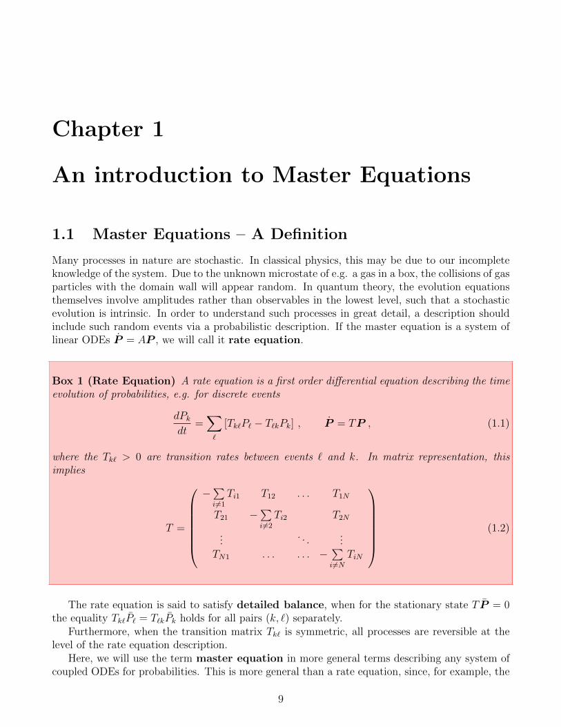
Box 1 (Rate Equation) A rate equation is a first order differential equation describing the timeevolution of probabilities, e.g. for discrete events
dPkdt
=∑`
[Tk`P` − T`kPk] , P = TP , (1.1)
where the Tk` > 0 are transition rates between events ` and k. In matrix representation, thisimplies
T =
−∑i 6=1
Ti1 T12 . . . T1N
T21 −∑i 6=2
Ti2 T2N
.... . .
...TN1 . . . . . . −
∑i 6=N
TiN
(1.2)
The rate equation is said to satisfy detailed balance, when for the stationary state T P = 0the equality Tk`P` = T`kPk holds for all pairs (k, `) separately.
Furthermore, when the transition matrix Tk` is symmetric, all processes are reversible at thelevel of the rate equation description.
Here, we will use the term master equation in more general terms describing any system ofcoupled ODEs for probabilities. This is more general than a rate equation, since, for example, the
9
10 CHAPTER 1. AN INTRODUCTION TO MASTER EQUATIONS
Markovian quantum master equation does in general not only involve probabilities (diagonals ofthe density matrix) but also coherences (off-diagonals).
It is straightforward to show that rate equations conserve the total probability∑k
dPkdt
=∑k`
(Tk`P` − T`kPk) =∑k`
(T`kPk − T`kPk) = 0 . (1.3)
Beyond this, all probabilities must remain positive, which is also respected by a normal rateequation: Evidently, the solution of a rate equation is continuous, such that when initializedwith valid probabilities 0 ≤ Pi(0) ≤ 1 all probabilities are non-negative initially. Let us assumethat after some time, the probability Pk it the first to approach zero (such that all others arenon-negative). Its time-derivative is then always non-negative
dPkdt
∣∣∣∣Pk=0
= +∑`
Tk`P` ≥ 0 , (1.4)
which implies that Pk = 0 is repulsive, and negative probabilities are prohibited.Finally, the probabilities must remain smaller than one throughout the evolution. This however
follows immediately from∑
k Pk = 1 and Pk ≥ 0 by contradiction.In conclusion, a rate equation of the form (1.1) automatically preserves the sum of probabilities
and also keeps 0 ≤ Pi(t) ≤ 1 – a valid initialization provided. That is, under the evolution of arate equation, probabilities remain probabilities.
1.1.1 Example 1: Fluctuating two-level system
Let us consider a system of two possible events, to which we associate the time-dependent proba-bilities P0(t) and P1(t). These events could for example be the two conformations of a molecule,the configurations of a spin, the two states of an excitable atom, etc. To introduce some dynamics,let the transition rate from 0→ 1 be denoted by T10 > 0 and the inverse transition rate 1→ 0 bedenoted by T01 > 0. The associated master equation is then given by
d
dt
(P0
P1
)=
(−T10 +T01
+T10 −T01
)(P0
P1
)(1.5)
Exercise 1 (Temporal Dynamics of a two-level system) (1 point)Calculate the solution of Eq. (1.5). What is the stationary state?
1.1.2 Example 2: Interacting quantum dots
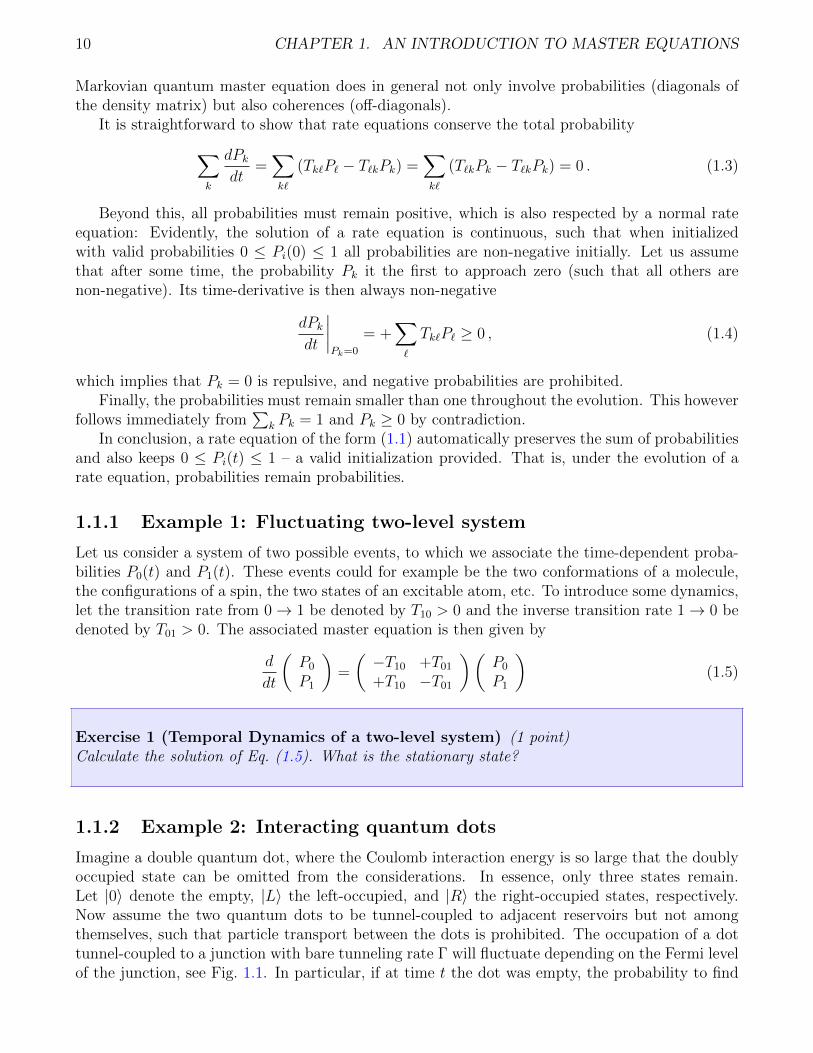
Imagine a double quantum dot, where the Coulomb interaction energy is so large that the doublyoccupied state can be omitted from the considerations. In essence, only three states remain.Let |0〉 denote the empty, |L〉 the left-occupied, and |R〉 the right-occupied states, respectively.Now assume the two quantum dots to be tunnel-coupled to adjacent reservoirs but not amongthemselves, such that particle transport between the dots is prohibited. The occupation of a dottunnel-coupled to a junction with bare tunneling rate Γ will fluctuate depending on the Fermi levelof the junction, see Fig. 1.1. In particular, if at time t the dot was empty, the probability to find
1.1. MASTER EQUATIONS – A DEFINITION 11
Figure 1.1: A single quantum dot coupled to a single junction, where the electronic occupation ofenergy levels is well approximated by a Fermi distribution.
an electron in the dot at time t+ ∆t is roughly given by Γ∆tf(ε) with the Fermi function definedas
f(ω) =1
eβ(ω−µ) + 1, (1.6)
where β denotes the inverse temperature and µ the chemical potential of the junction. Thetransition rate is thus given by the tunneling rate Γ multiplied by the probability to have anelectron in the junction at the required energy ε ready to jump into the system. The inverseprobability to find an initially filled dot empty reads Γ∆t [1− f(ε)], i.e., here one has to muliplythe bare tunneling rate with the probability to have a free slot at energy ε in the junction. Applyingthis recipe to every dot separately we obtain for the total rate matrix
T = ΓL
−fL 1− fL 0+fL −(1− fL) 0
0 0 0
+ ΓR
−fR 0 1− fR0 0 0
+fR 0 −(1− fR)
. (1.7)
In fact, a microscopic derivation can be used to confirm the above-mentioned assumptions, andthe parameters fα become the Fermi functions
fα =1
eβα(εα−µα) + 1(1.8)
with inverse temperature βα, chemical potentials µα, and dot level energy εα.
Exercise 2 (Detailed balance) Determine whether the rate matrix (1.7) obeys detailed balance.
1.1.3 Example 3: Diffusion Equation
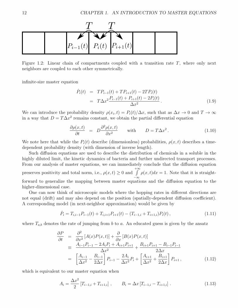
Consider an infinite chain of coupled compartments as displayed in Fig. 1.2. Now suppose thatalong the chain, a molecule may move from one compartment to another with a transition rateT that is unbiased, i.e., symmetric in all directions. The evolution of probabilities obeys the
12 CHAPTER 1. AN INTRODUCTION TO MASTER EQUATIONS
Figure 1.2: Linear chain of compartments coupled with a transition rate T , where only nextneighbors are coupled to each other symmetrically.
infinite-size master equation
Pi(t) = TPi−1(t) + TPi+1(t)− 2TPi(t)
= T∆x2Pi−1(t) + Pi+1(t)− 2Pi(t)
∆x2. (1.9)
We can introduce the probability density ρ(xi, t) = Pi(t)/∆x, such that as ∆x → 0 and T → ∞in a way that D = T∆x2 remains constant, we obtain the partial differential equation
∂ρ(x, t)
∂t= D
∂2ρ(x, t)
∂x2with D = T∆x2 . (1.10)
We note here that while the Pi(t) describe (dimensionless) probabilities, ρ(x, t) describes a time-dependent probability density (with dimension of inverse length).
Such diffusion equations are used to describe the distribution of chemicals in a soluble in thehighly diluted limit, the kinetic dynamics of bacteria and further undirected transport processes.From our analysis of master equations, we can immediately conclude that the diffusion equation
preserves positivity and total norm, i.e., ρ(x, t) ≥ 0 and+∞∫−∞
ρ(x, t)dx = 1. Note that it is straight-
forward to generalize the mapping between master equations and the diffusion equation to thehigher-dimensional case.
One can now think of microscopic models where the hopping rates in different directions arenot equal (drift) and may also depend on the position (spatially-dependent diffusion coefficient).A corresponding model (in next-neighbor approximation) would be given by
Pi = Ti,i−1Pi−1(t) + Ti,i+1Pi+1(t)− (Ti−1,i + Ti+1,i)Pi(t) , (1.11)
where Ta,b denotes the rate of jumping from b to a. An educated guess is given by the ansatz
∂P
∂t=
∂2
∂x2[A(x)P (x, t)] +
∂
∂x[B(x)P (x, t)]
≡ Ai−1Pi−1 − 2AiPi + Ai+1Pi+1
∆x2+Bi+1Pi+1 −Bi−1Pi−1
2∆x
=
[Ai−1
∆x2− Bi−1
2∆x
]Pi−1 −
2Ai∆x2
Pi +
[Ai+1
∆x2+Bi+1
2∆x
]Pi+1 , (1.12)
which is equivalent to our master equation when
Ai =∆x2
2[Ti−1,i + Ti+1,i] , Bi = ∆x [Ti−1,i − Ti+1,i] . (1.13)
1.2. DENSITY MATRIX FORMALISM 13
We conclude that the Fokker-Planck equation
∂ρ
∂t=
∂2
∂x2[A(x)ρ(x, t)] +
∂
∂x[B(x)ρ(x, t)] (1.14)
with A(x) ≥ 0 preserves norm and positivity of the probability distribution ρ(x, t).
Exercise 3 (Reaction-Diffusion Equation) (1 point)Along a linear chain of compartments consider the master equation for two species
Pi = T [Pi−1(t) + Pi+1(t)− 2Pi(t)]− γPi(t) ,pi = τ [pi−1(t) + pi+1(t)− 2pi(t)] + γPi(t),
where Pi(t) may denote the concentration of a molecule that irreversibly reacts with chemicals inthe soluble to an inert form characterized by pi(t). To which partial differential equation does themaster equation map?
In some cases, the probabilities may not only depend on the probabilities themselves, butalso on external parameters, which appear then in the master equation. Here, we will use theterm master equation for any equation describing the time evolution of probabilities, i.e., auxiliaryvariables may appear in the master equation.
1.2 Density Matrix Formalism
1.2.1 Density Matrix
Suppose one wants to describe a quantum system, where the system state is not exactly known.That is, there is an ensemble of known normalized states |Φi〉, but there is uncertainty in whichof these states the system is. Such systems can be conveniently described by the density matrix.
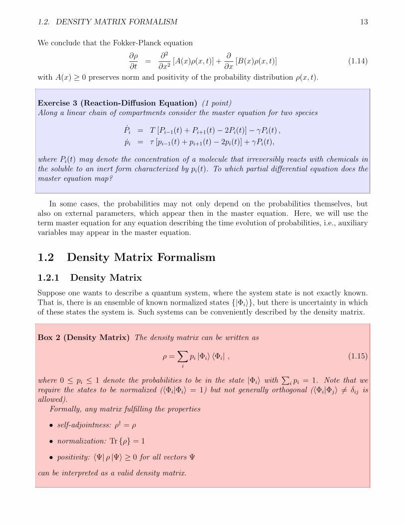
Box 2 (Density Matrix) The density matrix can be written as
ρ =∑i
pi |Φi〉 〈Φi| , (1.15)
where 0 ≤ pi ≤ 1 denote the probabilities to be in the state |Φi〉 with∑
i pi = 1. Note that werequire the states to be normalized (〈Φi|Φi〉 = 1) but not generally orthogonal (〈Φi|Φj〉 6= δij isallowed).
Formally, any matrix fulfilling the properties
• self-adjointness: ρ† = ρ
• normalization: Tr ρ = 1
• positivity: 〈Ψ| ρ |Ψ〉 ≥ 0 for all vectors Ψ
can be interpreted as a valid density matrix.
14 CHAPTER 1. AN INTRODUCTION TO MASTER EQUATIONS
For a pure state one has pi = 1 and thereby ρ = |Φi〉 〈Φi|. Evidently, a density matrix is pureif and only if ρ = ρ2.
The expectation value of an operator for a known state |Ψ〉
〈A〉 = 〈Ψ|A |Ψ〉 (1.16)
can be obtained conveniently from the corresponding pure density matrix ρ = |Ψ〉 〈Ψ| by simplycomputing the trace
〈A〉 ≡ Tr Aρ = Tr ρA = Tr A |Ψ〉 〈Ψ|
=∑n
〈n|A |Ψ〉 〈Ψ|n〉 = 〈Ψ|
(∑n
|n〉 〈n|
)A |Ψ〉
= 〈Ψ|A |Ψ〉 . (1.17)
When the state is not exactly known but its probability distribution, the expectation value isobtained by computing the weighted average
〈A〉 =∑i
Pi 〈Φi|A |Φi〉 , (1.18)
where Pi denotes the probability to be in state |Φi〉. The definition of obtaining expectation valuesby calculating traces of operators with the density matrix is also consistent with mixed states
〈A〉 ≡ Tr Aρ = Tr
A∑i
pi |Φi〉 〈Φi|
=∑i
piTr A |Φi〉 〈Φi|
=∑i
pi∑n
〈n|A |Φi〉 〈Φi|n〉 =∑i
pi 〈Φi|
(∑n
|n〉 〈n|
)A |Φi〉
=∑i
pi 〈Φi|A |Φi〉 . (1.19)
Exercise 4 (Superposition vs Localized States) (1 point)Calculate the density matrix for a statistical mixture in the states |0〉 and |1〉 with probabilityp0 = 3/4 and p1 = 1/4. What is the density matrix for a statistical mixture of the superpositionstates |Ψa〉 =
√3/4 |0〉+
√1/4 |1〉 and |Ψb〉 =
√3/4 |0〉−
√1/4 |1〉 with probabilities pa = pb = 1/2.
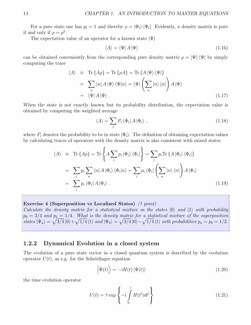
1.2.2 Dynamical Evolution in a closed system
The evolution of a pure state vector in a closed quantum system is described by the evolutionoperator U(t), as e.g. for the Schrodinger equation∣∣∣Ψ(t)
⟩= −iH(t) |Ψ(t)〉 (1.20)
the time evolution operator
U(t) = τ exp
−i
t∫0
H(t′)dt′
(1.21)
1.2. DENSITY MATRIX FORMALISM 15
may be defined as the solution to the operator equation
U(t) = −iH(t)U(t) . (1.22)
For constant H(0) = H, we simply have the solution U(t) = e−iHt. Similarly, a pure-state densitymatrix ρ = |Ψ〉 〈Ψ| would evolve according to the von-Neumann equation
ρ = −i [H(t), ρ(t)] (1.23)
with the formal solution ρ(t) = U(t)ρ(0)U †(t), compare Eq. (1.21).When we simply apply this evolution equation to a density matrix that is not pure, we obtain
ρ(t) =∑i
piU(t) |Φi〉 〈Φi|U †(t) , (1.24)
i.e., transitions between the (now time-dependent) state vectors |Φi(t)〉 = U(t) |Φi〉 are impossiblewith unitary evolution. This means that the von-Neumann evolution equation does yield the samedynamics as the Schrodinger equation if it is restarted on different initial states.
Exercise 5 (Preservation of density matrix properties by unitary evolution) (1 point)Show that the von-Neumann (1.23) equation preserves self-adjointness, trace, and positivity of thedensity matrix.
Also the Measurement process can be generalized similarly. For a quantum state |Ψ〉, measure-ments are described by a set of measurement operators Mm, each corresponding to a certainmeasurement outcome, and with the completeness relation
∑mM
†mMm = 1. The probability of
obtaining result m is given by
pm = 〈Ψ|M †mMm |Ψ〉 (1.25)
and after the measurement with outcome m, the quantum state is collapsed
|Ψ〉 m→ Mm |Ψ〉√〈Ψ|M †
mMm |Ψ〉. (1.26)
The projective measurement is just a special case of that with Mm = |m〉 〈m|.
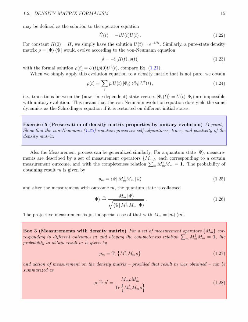
Box 3 (Measurements with density matrix) For a set of measurement operators Mm cor-responding to different outcomes m and obeying the completeness relation
∑mM
†mMm = 1, the
probability to obtain result m is given by
pm = TrM †
mMmρ
(1.27)
and action of measurement on the density matrix – provided that result m was obtained – can besummarized as
ρm→ ρ′ =
MmρM†m
TrM †
mMmρ (1.28)
16 CHAPTER 1. AN INTRODUCTION TO MASTER EQUATIONS
It is therefore straightforward to see that description by Schrodinger equation or von-Neumannequation with the respective measurement postulates are equivalent. The density matrix formal-ism conveniently includes statistical mixtures in the description but at the cost of quadraticallyincreasing the number of state variables.
Exercise 6 (Preservation of density matrix properties by measurement) (1 point)Show that the measurement postulate preserves self-adjointness, trace, and positivity of the densitymatrix.
1.2.3 Most general evolution
Finally, we mention here that the most general evolution preserving all the nice properties of adensity matrix is the so-called Kraus map. A density matrix ρ (hermitian, positive definite, andwith trace one) can be mapped to another density matrix ρ′ via
ρ′ =∑αβ
γαβAαρA†β , with
∑αβ
γαβA†βAα = 1 , (1.29)
where the prefactors γαβ form a hermitian (γαβ = γ∗βα) and positive definite (∑
αβ x∗αγαβxβ ≥ 0 or
equivalently all eigenvalues of (γαβ) are non-negative) matrix. It is straightforward to see that theabove map preserves trace and hermiticity of the density matrix. In addition, ρ′ also inherits thepositivity from ρ =
∑n Pn |n〉 〈n|
〈Ψ| ρ′ |Ψ〉 =∑αβ
γαβ 〈Ψ|AαρA†β |Ψ〉 =∑n
Pn∑αβ
γαβ 〈Ψ|Aα |n〉 〈n|A†β |Ψ〉
=∑n
Pn︸︷︷︸≥0
∑αβ
(〈n|A†α |Ψ〉
)∗γαβ 〈n|A†β |Ψ〉︸ ︷︷ ︸
≥0
≥ 0 . (1.30)
Since the matrix γαβ is hermitian, it can be diagonalized by a suitable unitary transformation, andwe introduce the new operators Aα =
∑α′ Uαα′Kα′
ρ′ =∑αβ
∑α′β′
γαβUαα′Kα′ρU∗ββ′K
†β′ =
∑α′β′
Kα′ρK†β′
∑αβ
Uαα′γαβU∗ββ′︸ ︷︷ ︸
γα′δα′β′
=∑α
γαKαρK†α , (1.31)
where γα ≥ 0 represent the eigenvalues of the matrix (γαβ). Since these are by constructionpositive, we introduce further new operators Kα =
√γαKα to obtain the simplest representation
of a Kraus map.
Box 4 (Kraus map) The map
ρ(t+ ∆t) =∑α
Kα(t,∆t)ρ(t)K†α(t,∆t) (1.32)
1.2. DENSITY MATRIX FORMALISM 17
with Kraus operators Kα(t,∆t) obeying the relation∑
αK†α(t,∆t)Kα(t,∆t) = 1 preserves her-
miticity, trace, and positivity of the density matrix.
Obviously, both unitary evolution and evolution under measurement are just special cases of aKraus map. Though Kraus maps are heavily used in quantum information, they are not often veryeasy to interpret. For example, it is not straightforward to identify the unitary and the non-unitarypart induced the Kraus map.
1.2.4 Lindblad master equation
Any dynamical evolution equation for the density matrix should (at least in some approximatesense) preserve its interpretation as density matrix, i.e., trace, hermiticity, and positivity mustbe preserved. By construction, the measurement postulate and unitary evolution preserve theseproperties. However, more general evolutions are conceivable. If we constrain ourselves to masterequations that are local in time and have constant coefficients, the most general evolution thatpreserves trace, self-adjointness, and positivity of the density matrix is given by a Lindblad form.
Box 5 (Lindblad form) In an N-dimensional system Hilbert space, a master equation of Lind-blad form has the structure
ρ = Lρ = −i [H, ρ] +N2−1∑α,β=1
γαβ
(AαρA
†β −
1
2
A†βAα, ρ
), (1.33)
where the hermitian operator H = H† can be interpreted as an effective Hamiltonian and γαβ = γ∗βαis a positive semidefinite matrix, i.e., it fulfills
∑αβ
x∗αγαβxβ ≥ 0 for all vectors x (or, equivalently
that all eigenvalues of (γαβ) are non-negative λi ≥ 0).
Exercise 7 (Trace and Hermiticity preservation by Lindblad forms) (1 points)Show that the Lindblad form master equation preserves trace and hermiticity of the density matrix.
The Lindblad type master equation can be written in simpler form: As the dampening ma-trix γ is hermitian, it can be diagonalized by a suitable unitary transformation U , such that∑
αβ Uα′αγαβ(U †)ββ′ = δα′β′γα′ with γα ≥ 0 representing its non-negative eigenvalues. Using thisunitary operation, a new set of operators can be defined via Aα =
∑α′ Uα′αLα′ . Inserting this
18 CHAPTER 1. AN INTRODUCTION TO MASTER EQUATIONS
decomposition in the master equation, we obtain
ρ = −i [H, ρ] +N2−1∑α,β=1
γαβ
(AαρA
†β −
1
2
A†βAα, ρ
)
= −i [H, ρ] +∑α′,β′
[∑αβ
γαβUα′αU∗β′β
](Lα′ρL
†β′ −
1
2
L†β′Lα′ , ρ
)= −i [H, ρ] +
∑α
γα
(LαρL
†α −
1
2
L†αLα, ρ
), (1.34)
where γα denote the N2 − 1 non-negative eigenvalues of the dampening matrix. Furthermore, wecan in principle absorb the γα in the Lindblad operators Lα =
√γαLα, such that another form of
a Lindblad master equation would be
ρ = −i [H, ρ] +∑α
(LαρL
†α −
1
2
L†αLα, ρ
). (1.35)
Evidently, the representation of a master equation is not unique.Any other unitary operation would lead to a different non-diagonal form of γαβ which however
describes the same master equation. In addition, we note here that the master equation is notonly invariant to unitary transformations of the operators Aα, but in the diagonal representationalso to inhomogeneous transformations of the form
Lα → L′α = Lα + aα
H → H ′ = H +1
2i
∑α
γα(a∗αLα − aαL†α
)+ b , (1.36)
with complex numbers aα and a real number b. The numbers aα can be chosen such that theLindblad operators are traceless Tr Lα = 0, which is a popular convention. Choosing b simplycorresponds to gauging the energy of the system.
Exercise 8 (Shift invariance) (1 points)Show the invariance of the diagonal representation of a Lindblad form master equation (1.34) withrespect to the transformation (1.36).
We would like to demonstrate the preservation of positivity here. Since preservation of her-miticity follows directly from the Lindblad form, we can – at any time – formally write the densitymatrix in its spectral representation
ρ(t) =∑j
Pj(t) |Ψj(t)〉 〈Ψj(t)| (1.37)
with probabilities Pj(t) ∈ R (we still have to show that these remain positive) and time-dependentorthonormal eigenstates obeying unitary evolution∣∣∣Ψj(t)
⟩= −iK(t) |Ψj(t)〉 , K(t) = K†(t) . (1.38)
1.2. DENSITY MATRIX FORMALISM 19
Exercise 9 (Evolution of Eigenstates is Unitary) Show that orthonormality of time-dependent eigenstates implies unitary evolution, i.e., a hermitian operator K(t).
The hermitian conjugate equation also implies that⟨
Ψj
∣∣∣ = +i 〈Ψj|K. Therefore, its time-
derivative becomes
ρ =∑j
[Pj |Ψj〉 〈Ψj| − iPjK |Ψj〉 〈Ψj|+ iPj |Ψj〉 〈Ψj|K
], (1.39)
and sandwiching the density matrix yields to the cancellation of two terms, such that 〈Ψj(t)| ρ |Ψj(t)〉 =Pj(t). On the other hand, we can also use the Lindblad equation to obtain
Pj = −i 〈Ψj|H |Ψj〉Pj + iPj 〈Ψj|H |Ψj〉
+∑α
γα
[〈Ψj|Lα(
∑k
Pk |Ψk〉 〈Ψk|)L†α |Ψj〉 − 〈Ψj|L†αLα |Ψj〉Pj
]
=
(∑k
∑α
γα|〈Ψj|Lα |Ψk〉|2Pk
)−
(∑α
γα 〈Ψj|L†αLα |Ψj〉
)Pj . (1.40)
This is nothing but a rate equation with positive but time-dependent transition rates
Rk→j(t) =∑α
γα|〈Ψj(t)|Lα |Ψk(t)〉|2 ≥ 0 , (1.41)
and with our arguments from Sec. 1.1 it follows that the positivity of the eigenvalues Pj(t) isgranted, a valid initialization provided. Unfortunately, the basis within which this simple rateequation holds is time-dependent and also only known after solving the master equation anddiagonalizing the solution. It is therefore not very practical in most occasions.
1.2.5 Example: Master Equation for a cavity in a thermal bath
Consider the Lindblad form master equation
ρ = −i[Ωa†a, ρ
]+ Γ(1 + nB)
[aρa† − 1
2a†aρ− 1
2ρa†a
]+ΓnB
[a†ρa− 1
2aa†ρ− 1
2ρaa†
], (1.42)
with bosonic operators[a, a†
]= 1 and Bose-Einstein bath occupation nB =
[eβΩ − 1
]−1and cavity
frequency Ω. In Fock-space representation, these operators act as a† |n〉 =√n+ 1 |n+ 1〉 (where
0 ≤ n <∞), such that the above master equation couples only the diagonals of the density matrixρn = 〈n| ρ |n〉 to each other. This is directly visible by sandwhiching the master equation with〈n| . . . |n〉
ρn = Γ(1 + nB) [(n+ 1)ρn+1 − nρn] + ΓnB [nρn−1 − (n+ 1)ρn]
= ΓnBnρn−1 − Γ [n+ (2n+ 1)nB] ρn + Γ(1 + nB)(n+ 1)ρn+1 , (1.43)
20 CHAPTER 1. AN INTRODUCTION TO MASTER EQUATIONS
which shows that the rate equation arising for the diagonals even has a simple tri-diagonal form.That makes it particularly easy to calculate its stationary state recursively, since the boundarysolution nBρ0 = (1 + nB)ρ1 implies for all n the relation
ρn+1
ρn=
nB1 + nB
= e−βΩ , (1.44)
i.e., the stationary state is a thermalized Gibbs state with the same temperature as the reservoir.
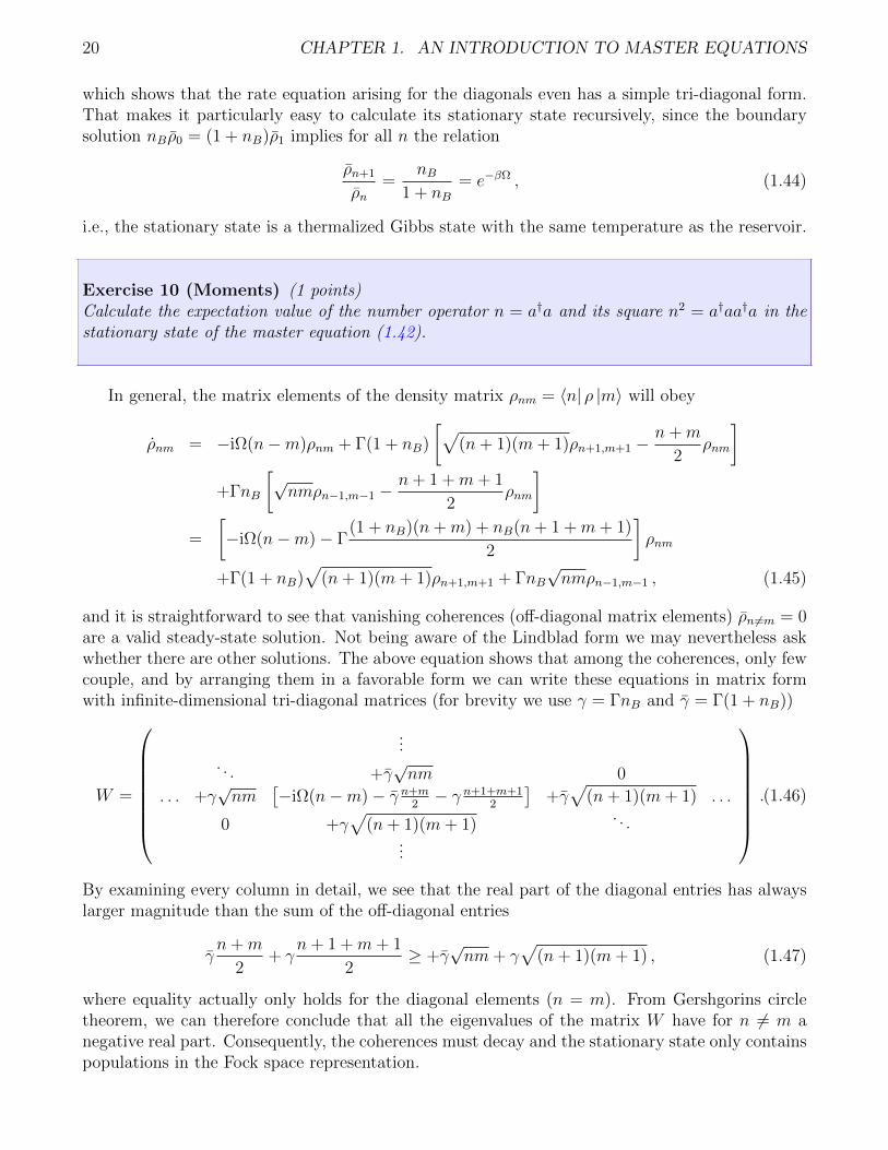
Exercise 10 (Moments) (1 points)Calculate the expectation value of the number operator n = a†a and its square n2 = a†aa†a in thestationary state of the master equation (1.42).
In general, the matrix elements of the density matrix ρnm = 〈n| ρ |m〉 will obey
ρnm = −iΩ(n−m)ρnm + Γ(1 + nB)
[√(n+ 1)(m+ 1)ρn+1,m+1 −
n+m
2ρnm
]+ΓnB
[√nmρn−1,m−1 −
n+ 1 +m+ 1
2ρnm
]=
[−iΩ(n−m)− Γ
(1 + nB)(n+m) + nB(n+ 1 +m+ 1)
2
]ρnm
+Γ(1 + nB)√
(n+ 1)(m+ 1)ρn+1,m+1 + ΓnB√nmρn−1,m−1 , (1.45)
and it is straightforward to see that vanishing coherences (off-diagonal matrix elements) ρn 6=m = 0are a valid steady-state solution. Not being aware of the Lindblad form we may nevertheless askwhether there are other solutions. The above equation shows that among the coherences, only fewcouple, and by arranging them in a favorable form we can write these equations in matrix formwith infinite-dimensional tri-diagonal matrices (for brevity we use γ = ΓnB and γ = Γ(1 + nB))
W =
.... . . +γ
√nm 0
. . . +γ√nm
[−iΩ(n−m)− γ n+m
2− γ n+1+m+1
2
]+γ√
(n+ 1)(m+ 1) . . .
0 +γ√
(n+ 1)(m+ 1). . .
...
.(1.46)
By examining every column in detail, we see that the real part of the diagonal entries has alwayslarger magnitude than the sum of the off-diagonal entries
γn+m
2+ γ
n+ 1 +m+ 1
2≥ +γ
√nm+ γ
√(n+ 1)(m+ 1) , (1.47)
where equality actually only holds for the diagonal elements (n = m). From Gershgorins circletheorem, we can therefore conclude that all the eigenvalues of the matrix W have for n 6= m anegative real part. Consequently, the coherences must decay and the stationary state only containspopulations in the Fock space representation.
1.2. DENSITY MATRIX FORMALISM 21
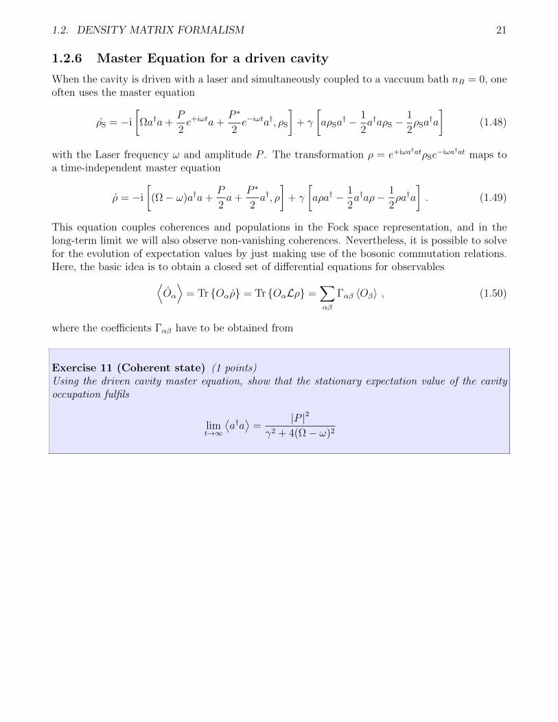
1.2.6 Master Equation for a driven cavity
When the cavity is driven with a laser and simultaneously coupled to a vaccuum bath nB = 0, oneoften uses the master equation
ρS = −i
[Ωa†a+
P
2e+iωta+
P ∗
2e−iωta†, ρS
]+ γ
[aρSa
† − 1
2a†aρS −
1
2ρSa
†a
](1.48)
with the Laser frequency ω and amplitude P . The transformation ρ = e+iωa†atρSe−iωa†at maps to
a time-independent master equation
ρ = −i
[(Ω− ω)a†a+
P
2a+
P ∗
2a†, ρ
]+ γ
[aρa† − 1
2a†aρ− 1
2ρa†a
]. (1.49)
This equation couples coherences and populations in the Fock space representation, and in thelong-term limit we will also observe non-vanishing coherences. Nevertheless, it is possible to solvefor the evolution of expectation values by just making use of the bosonic commutation relations.Here, the basic idea is to obtain a closed set of differential equations for observables⟨
Oα
⟩= Tr Oαρ = Tr OαLρ =
∑αβ
Γαβ 〈Oβ〉 , (1.50)
where the coefficients Γαβ have to be obtained from
Exercise 11 (Coherent state) (1 points)Using the driven cavity master equation, show that the stationary expectation value of the cavityoccupation fulfils
limt→∞
⟨a†a⟩
=|P |2
γ2 + 4(Ω− ω)2

22 CHAPTER 1. AN INTRODUCTION TO MASTER EQUATIONS
Chapter 2
Obtaining a Master Equation
2.1 Mathematical Prerequisites
Master equations are often used to describe the dynamics of systems interacting with one or manylarge reservoirs (baths). To derive them from microscopic models – including the Hamiltonian ofthe full system – requires to review some basic mathematical concepts.
2.1.1 Tensor Product
The greatest advantage of the density matrix formalism is visible when quantum systems composedof several subsystems are considered. Roughly speaking, the tensor product represents a way toconstruct a larger vector space from two (or more) smaller vector spaces.
Box 6 (Tensor Product) Let V and W be Hilbert spaces (vector spaces with scalar product) ofdimension m and n with basis vectors |v〉 and |w〉, respectively. Then V ⊗ W is a Hilbertspace of dimension m · n, and a basis is spanned by |v〉 ⊗ |w〉, which is a set combining everybasis vector of V with every basis vector of W .
Mathematical properties
• Bilinearity (z1 |v1〉+ z2 |v2〉)⊗ |w〉 = z1 |v1〉 ⊗ |w〉+ z2 |v2〉 ⊗ |w〉
• operators acting on the combined Hilbert space A⊗B act on the basis states as (A⊗B)(|v〉⊗|w〉) = (A |v〉)⊗ (B |w〉)
• any linear operator on V ⊗W can be decomposed as C =∑
i ciAi ⊗Bi
• the scalar product is inherited in the natural way, i.e., one has for |a〉 =∑
ij aij |vi〉 ⊗ |wj〉and |b〉 =
∑k` bk` |vk〉⊗|w`〉 the scalar product 〈a|b〉 =
∑ijk` a
∗ijbk` 〈vi|vk〉 〈wj|w`〉 =
∑ij a∗ijbij
If more than just two vector spaces are combined to form a larger vector space, the dimension ofthe joint vector space grows rapidly, as e.g. exemplified by the case of a qubit: Its Hilbert space isjust spanned by two vectors |0〉 and |1〉. The joint Hilbert space of two qubits is four-dimensional, ofthree qubits 8-dimensional, and of n qubits 2n-dimensional. Eventually, this exponential growth ofthe Hilbert space dimension for composite quantum systems is at the heart of quantum computing.
23
24 CHAPTER 2. OBTAINING A MASTER EQUATION
Exercise 12 (Tensor Products of Operators) (1 points)Let σ denote the Pauli matrices, i.e.,
σ1 =
(0 +1
+1 0
)σ2 =
(0 −i
+i 0
)σ3 =
(+1 00 −1
)Compute the trace of the operator
Σ = a1⊗ 1 +3∑i=1
αiσi ⊗ 1 +
3∑j=1
βj1⊗ σj +3∑
i,j=1
aijσi ⊗ σj .
Since the scalar product is inherited, this typically enables a convenient calculation of the tracein case of a few operator decomposition, e.g., for just two operators
Tr A⊗B =∑nA,nB
〈nA, nB|A⊗B |nA, nB〉
=
[∑nA
〈nA|A |nA〉
][∑nB
〈nB|B |nB〉
]= TrAATrBB , (2.1)
where TrA/B denote the trace in the Hilbert space of A and B, respectively.
2.1.2 The partial trace
For composite systems, it is usually not necessary to keep all information of the complete systemin the density matrix. Rather, one would like to have a density matrix that encodes all theinformation on a particular subsystem only. Obviously, the map ρ → TrB ρ to such a reduceddensity matrix should leave all expectation values of observables A acting only on the consideredsubsystem invariant, i.e.,
Tr A⊗ 1ρ = Tr ATrB ρ . (2.2)
If this basic condition was not fulfilled, there would be no point in defining such a thing as areduced density matrix: Measurement would yield different results depending on the Hilbert spaceof the experimenters feeling.
Box 7 (Partial Trace) Let |a1〉 and |a2〉 be vectors of state space A and |b1〉 and |b2〉 vectors ofstate space B. Then, the partial trace over state space B is defined via
TrB |a1〉 〈a2| ⊗ |b1〉 〈b2| = |a1〉 〈a2|Tr |b1〉 〈b2| . (2.3)
The partial trace is linear, such that the partial trace of arbitrary operators is calculatedsimilarly. By choosing the |aα〉 and |bγ〉 as an orthonormal basis in the respective Hilbert space,
2.2. DERIVATIONS FOR OPEN QUANTUM SYSTEMS 25
one may therefore calculate the most general partial trace via
TrB C = TrB
∑αβγδ
cαβγδ |aα〉 〈aβ| ⊗ |bγ〉 〈bδ|
=
∑αβγδ
cαβγδTrB |aα〉 〈aβ| ⊗ |bγ〉 〈bδ|
=∑αβγδ
cαβγδ |aα〉 〈aβ|Tr |bγ〉 〈bδ|
=∑αβγδ
cαβγδ |aα〉 〈aβ|∑ε
〈bε|bγ〉 〈bδ|bε〉
=∑αβ
[∑γ
cαβγγ
]|aα〉 〈aβ| . (2.4)
The definition 7 is the only linear map that respects the invariance of expectation values.
Exercise 13 (Partial Trace) (1 points)Compute the partial trace of a pure density matrix ρ = |Ψ〉 〈Ψ| in the bipartite state
|Ψ〉 =1√2
(|01〉+ |10〉) ≡ 1√2
(|0〉 ⊗ |1〉+ |1〉 ⊗ |0〉)
2.2 Derivations for Open Quantum Systems
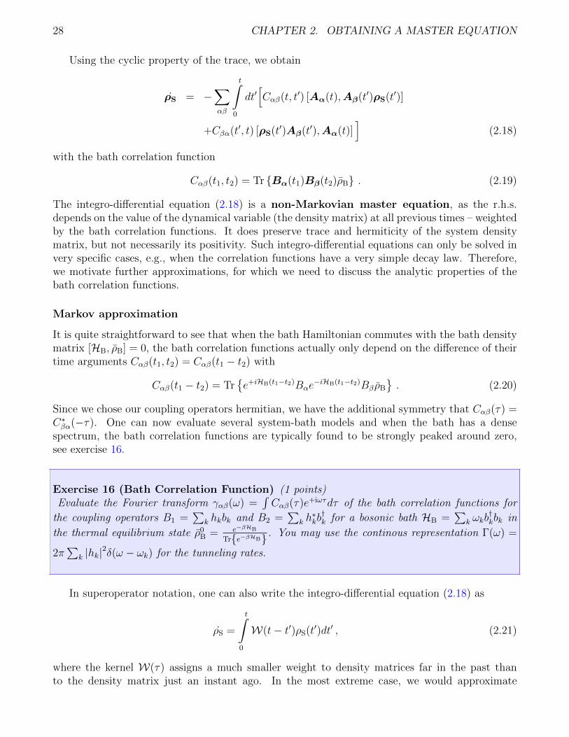
In some cases, it is possible to derive a master equation rigorously based only on a few assumptions.Open quantum systems for example are mostly treated as part of a much larger closed quantumsystem (the union of system and bath), where the partial trace is used to eliminate the unwanted(typically many) degrees of freedom of the bath, see Fig. 2.1. Technically speaking, we will consider
Figure 2.1: An open quantum system can be conceived as being part of a larger closed quantumsystem, where the system part (HS) is coupled to the bath (HB) via the interaction HamiltonianHI.
Hamiltonians of the form
H = HS ⊗ 1 + 1⊗HB +HI , (2.5)
26 CHAPTER 2. OBTAINING A MASTER EQUATION
where the system and bath Hamiltonians act only on the system and bath Hilbert space, respec-tively. In contrast, the interaction Hamiltonian acts on both Hilbert spaces
HI =∑α
Aα ⊗Bα , (2.6)
where the summation boundaries are in the worst case limited by the dimension of the systemHilbert space. As we consider physical observables here, it is required that all Hamiltonians areself-adjoint.
Exercise 14 (Hermiticity of Couplings) (1 points)Show that it is always possible to choose hermitian coupling operators Aα = A†α and Bα = B†α usingthat HI = H†I .
2.2.1 Standard Quantum-Optical Derivation
Interaction Picture
When the interaction HI is small, it is justified to apply perturbation theory. The von-Neumannequation in the joint total quantum system
ρ = −i [HS ⊗ 1 + 1⊗HB +HI, ρ] (2.7)
describes the full evolution of the combined density matrix. This equation can be formally solved bythe unitary evolution ρ(t) = e−iHtρ0e
+iHt, which however is impractical to compute as H involvestoo many degrees of freedom.
Transforming to the interaction picture
ρ(t) = e+i(HS+HB)tρ(t)e−i(HS+HB)t , (2.8)
which will be denoted by bold symbols throughout, the von-Neumann equation transforms into
ρ = −i [HI(t),ρ] , (2.9)
where the in general time-dependent interaction Hamiltonian
HI(t) = e+i(HS+HB)tHIe−i(HS+HB)t =
∑α
e+iHStAαe−iHSt ⊗ e+iHBtBαe
−iHBt
=∑α
Aα(t)⊗Bα(t) (2.10)
allows to perform perturbation theory.Without loss of generality we will for simplicity assume here the case of hermitian coupling
operators Aα = A†α and Bα = B†α. One heuristic way to perform perturbation theory is to formallyintegrate Eq. (2.10) and to re-insert the result in the r.h.s. of Eq. (2.10). The time-derivative ofthe system density matrix is obtained by performing the partial trace
ρS = −iTrB [HI(t), ρ0] −t∫
0
TrB [HI(t), [HI(t′),ρ(t′)]] dt′ . (2.11)
This integro-differential equation is still exact but unfortunately not closed as the r.h.s. does notdepend on ρS but the full density matrix at all previous times.
2.2. DERIVATIONS FOR OPEN QUANTUM SYSTEMS 27
Born approximation
To close the above equation, we employ factorization of the initial density matrix
ρ0 = ρ0S ⊗ ρB (2.12)
together with perturbative considerations: Assuming that HI(t) = Oλ with λ beeing a smalldimensionless perturbation parameter (solely used for bookkeeping purposes here) and that theenvironment is so large such that it is hardly affected by the presence of the system, we mayformally expand the full density matrix
ρ(t) = ρS(t)⊗ ρB +Oλ , (2.13)
where the neglect of all higher orders is known as Born approximation. Eq. (2.11) demonstratesthat the Born approximation is equivalent to a perturbation theory in the interaction Hamiltonian
ρS = −iTrB [HI(t), ρ0] −t∫
0
TrB [HI(t), [HI(t′),ρS(t′)⊗ ρB]] dt′+Oλ3 . (2.14)
Using the decomposition of the interaction Hamiltonian (2.6), this obviously yields a closed equa-tion for the system density matrix
ρS = −i∑α
[Aα(t)ρ0
STr Bα(t)ρB − ρ0SAα(t)Tr ρBBα(t)
]−∑αβ
t∫0
[+Aα(t)Aβ(t′)ρS(t′)Tr Bα(t)Bβ(t′)ρB−Aα(t)ρS(t′)Aβ(t′)Tr Bα(t)ρBBβ(t′)−Aβ(t′)ρS(t′)Aα(t)Tr Bβ(t′)ρBBα(t)
+ρS(t′)Aβ(t′)Aα(t)Tr ρBBβ(t′)Bα(t)]dt′ . (2.15)
Without loss of generality, we proceed by assuming that the single coupling operator expectationvalue vanishes
Tr Bα(t)ρB = 0 . (2.16)
This situation can always be constructed by simultaneously modifying system Hamiltonian HS
and coupling operators Aα, see exercise 15.
Exercise 15 (Vanishing single-operator expectation values) (1 points)Show that by modifying system and interaction Hamiltonian
HS → HS +∑α
gαAα , Bα → Bα − gα1 (2.17)
one can construct a situation where Tr Bα(t)ρB = 0. Determine gα.
28 CHAPTER 2. OBTAINING A MASTER EQUATION
Using the cyclic property of the trace, we obtain
ρS = −∑αβ
t∫0
dt′[Cαβ(t, t′) [Aα(t),Aβ(t′)ρS(t′)]
+Cβα(t′, t) [ρS(t′)Aβ(t′),Aα(t)]]
(2.18)
with the bath correlation function
Cαβ(t1, t2) = Tr Bα(t1)Bβ(t2)ρB . (2.19)
The integro-differential equation (2.18) is a non-Markovian master equation, as the r.h.s.depends on the value of the dynamical variable (the density matrix) at all previous times – weightedby the bath correlation functions. It does preserve trace and hermiticity of the system densitymatrix, but not necessarily its positivity. Such integro-differential equations can only be solved invery specific cases, e.g., when the correlation functions have a very simple decay law. Therefore,we motivate further approximations, for which we need to discuss the analytic properties of thebath correlation functions.
Markov approximation
It is quite straightforward to see that when the bath Hamiltonian commutes with the bath densitymatrix [HB, ρB] = 0, the bath correlation functions actually only depend on the difference of theirtime arguments Cαβ(t1, t2) = Cαβ(t1 − t2) with
Cαβ(t1 − t2) = Tre+iHB(t1−t2)Bαe
−iHB(t1−t2)Bβ ρB
. (2.20)
Since we chose our coupling operators hermitian, we have the additional symmetry that Cαβ(τ) =C∗βα(−τ). One can now evaluate several system-bath models and when the bath has a densespectrum, the bath correlation functions are typically found to be strongly peaked around zero,see exercise 16.
Exercise 16 (Bath Correlation Function) (1 points)Evaluate the Fourier transform γαβ(ω) =
∫Cαβ(τ)e+iωτdτ of the bath correlation functions for
the coupling operators B1 =∑
k hkbk and B2 =∑
k h∗kb†k for a bosonic bath HB =
∑k ωkb
†kbk in
the thermal equilibrium state ρ0B = e−βHB
Tre−βHB . You may use the continous representation Γ(ω) =
2π∑
k |hk|2δ(ω − ωk) for the tunneling rates.
In superoperator notation, one can also write the integro-differential equation (2.18) as
ρS =
t∫0
W(t− t′)ρS(t′)dt′ , (2.21)
where the kernel W(τ) assigns a much smaller weight to density matrices far in the past thanto the density matrix just an instant ago. In the most extreme case, we would approximate
2.2. DERIVATIONS FOR OPEN QUANTUM SYSTEMS 29
Cαβ(t1, t2) ≈ Γαβδ(t1 − t2), but we will be cautious here and assume that only the density matrixvaries slower than the decay time of the bath correlation functions. Therefore, we replace in ther.h.s. ρS(t′)→ ρS(t) (first Markov approximation), which yields in Eq. (2.14)
ρS = −t∫
0
TrB [HI(t), [HI(t′),ρS(t)⊗ ρB]] dt′ (2.22)
This equation is often called Born-Redfield equation. It is time-local and preserves trace andhermiticity, but still has time-dependent coefficients (also when transforming back from the inter-action picture). We substitute τ = t− t′
ρS = −t∫
0
TrB [HI(t), [HI(t− τ),ρS(t)⊗ ρB]] dτ (2.23)
= −∑αβ
t∫0
Cαβ(τ) [Aα(t),Aβ(t− τ)ρS(t)] + Cβα(−τ) [ρS(t)Aβ(t− τ),Aα(t)] dτ
The problem that the r.h.s. still depends on time is removed by extending the integration boundsto infinity (second Markov approximation) – by the same reasoning that the bath correlationfunctions decay rapidly
ρS = −∞∫
0
TrB [HI(t), [HI(t− τ),ρS(t)⊗ ρB]] dτ . (2.24)
This equation is called the Markovian master equation, which in the original Schrodingerpicture
ρS = −i [HS, ρS(t)]−∑αβ
∞∫0
Cαβ(τ)[Aα, e
−iHSτAβe+iHSτρS(t)
]dτ
−∑αβ
∞∫0
Cβα(−τ)[ρS(t)e−iHSτAβe
+iHSτ , Aα]dτ (2.25)
is time-local, preserves trace and hermiticity, and has constant coefficients – best prerequisites fortreatment with established solution methods.
Exercise 17 (Properties of the Markovian Master Equation) (1 points)Show that the Markovian Master equation (2.25) preserves trace and hermiticity of the densitymatrix.
In addition, it can be obtained easily from the coupling Hamiltonian: We have so far not usedthat the coupling operators should be hermitian, and the above form is therefore also valid fornon-hermitian coupling operators.
There is just one problem left: In the general case, it is not of Lindblad form. Note thatthere are specific cases where the Markovian master equation is of Lindblad form, but these ratherinclude simple limits. Though this is sometimes considered a rather cosmetic drawback, it maylead to unphysical results such as negative probabilities.
30 CHAPTER 2. OBTAINING A MASTER EQUATION
Secular Approximation
To generally obtain a Lindblad type master equation, a further approximation is required. Thesecular approximation involves an averaging over fast oscillating terms, but in order to identifythe oscillating terms, it is necessary to at least formally calculate the interaction picture dynamicsof the system coupling operators. We begin by writing Eq. (2.25) in the interaction picture againexplicitly – now using the hermiticity of the coupling operators
ρS = −∞∫
0
∑αβ
Cαβ(τ) [Aα(t),Aβ(t− τ)ρS(t)] + h.c. dτ
= +
∞∫0
∑αβ
Cαβ(τ)∑a,b,c,d
|a〉 〈a|Aβ(t− τ) |b〉 〈b|ρS(t) |d〉 〈d|Aα(t) |c〉 〈c|
− |d〉 〈d|Aα(t) |c〉 〈c| |a〉 〈a|Aβ(t− τ) |b〉 〈b|ρS(t)dτ + h.c. , (2.26)
where we have introduced the system energy eigenbasis
HS |a〉 = Ea |a〉 . (2.27)
We can use this eigenbasis to make the time-dependence of the coupling operators in the interactionpicture explicit. To reduce the notational effort, we abbreviate Aabα = 〈a|Aα |b〉 and Lab = |a〉 〈b|.Then, the density matrix becomes
ρS = +
∞∫0
∑αβ
Cαβ(τ)∑a,b,c,d
e+i(Ea−Eb)(t−τ)e+i(Ed−Ec)tAabβ A
dcα LabρS(t)L†cd
−e+i(Ea−Eb)(t−τ)e+i(Ed−Ec)tAabβ Adcα L†cdLabρS(t)
dτ + h.c. ,
=∑αβ
∑a,b,c,d
∞∫0
Cαβ(τ)e+i(Eb−Ea)τdτe−i(Eb−Ea−(Ed−Ec))tAabβ (Acdα )∗LabρS(t)L†cd − L
†cdLabρS(t)
+h.c. (2.28)
The secular approximation now involves neglecting all terms that are oscillatory in time t(long-time average), i.e., we have
ρS =∑αβ
∑a,b,c,d
Γαβ(Eb − Ea)δEb−Ea,Ed−EcAabβ (Acdα )∗
+LabρS(t)L†cd − L†cdLabρS(t)
+∑αβ
∑a,b,c,d
Γ∗αβ(Eb − Ea)δEb−Ea,Ed−Ec(Aabβ )∗Acdα
+LcdρS(t)L†ab − ρS(t)L†abLcd
,(2.29)
where we have introduced the half-sided Fourier transform of the bath correlation functions
Γαβ(ω) =
∞∫0
Cαβ(τ)e+iωτdτ . (2.30)
This equation preserves trace, hermiticity, and positivity of the density matrix and hence all desiredproperties, since it is of Lindblad form (which will be shown later). Unfortunately, it is typically
2.2. DERIVATIONS FOR OPEN QUANTUM SYSTEMS 31
not so easy to obtain as it requires diagonalization of the system Hamiltonian first. By using thetransformations α↔ β, a↔ c, and b↔ d in the second line and also using that the δ-function issymmetric, we may rewrite the master equation as
ρS =∑αβ
∑a,b,c,d
[Γαβ(Eb − Ea) + Γ∗βα(Eb − Ea)
]δEb−Ea,Ed−EcA
abβ (Acdα )∗LabρS(t)L†cd
−∑αβ
∑a,b,c,d
Γαβ(Eb − Ea)δEb−Ea,Ed−EcAabβ (Acdα )∗L†cdLabρS(t)
−∑αβ
∑a,b,c,d
Γ∗βα(Eb − Ea)δEb−Ea,Ed−EcAabβ (Acdα )∗ρS(t)L†cdLab . (2.31)
We split the matrix-valued function Γαβ(ω) into hermitian and anti-hermitian parts
Γαβ(ω) =1
2γαβ(ω) +
1
2σαβ(ω) ,
Γ∗βα(ω) =1
2γαβ(ω)− 1
2σαβ(ω) , (2.32)
with hermitian γαβ(ω) = γ∗βα(ω) and anti-hermitian σαβ(ω) = −σ∗βα(ω). These new functions canbe interpreted as full even and odd Fourier transforms of the bath correlation functions
γαβ(ω) = Γαβ(ω) + Γ∗βα(ω) =
+∞∫−∞
Cαβ(τ)e+iωτdτ ,
σαβ(ω) = Γαβ(ω)− Γ∗βα(ω) =
+∞∫−∞
Cαβ(τ)sgn(τ)e+iωτdτ . (2.33)
Exercise 18 (Odd Fourier Transform) (1 points)Show that the odd Fourier transform σαβ(ω) may be obtained from the even Fourier transformγαβ(ω) by a Cauchy principal value integral
σαβ(ω) =i
πP
+∞∫−∞
γαβ(Ω)
ω − ΩdΩ .
In the master equation, these replacements lead to
ρS =∑αβ
∑a,b,c,d
γαβ(Eb − Ea)δEb−Ea,Ed−EcAabβ (Acdα )∗[LabρS(t)L†cd −
1
2
L†cdLab,ρS(t)
]−i∑αβ
∑a,b,c,d
1
2iσαβ(Eb − Ea)δEb−Ea,Ed−EcAabβ (Acdα )∗
[L†cdLab,ρS(t)
]=
∑αβ
∑a,b,c,d
γαβ(Eb − Ea)δEb−Ea,Ed−EcAabβ (Acdα )∗[LabρS(t)L†cd −
1
2
L†cdLab,ρS(t)
](2.34)
−i
[∑αβ
∑a,b,c
1
2iσαβ(Eb − Ec)δEb,EaAcbβ (Acaα )∗Lab,ρS(t)
].
32 CHAPTER 2. OBTAINING A MASTER EQUATION
To prove that we have a Lindblad form, it is easy to see first that the term in the commutator
HLS =∑αβ
∑a,b,c
1
2iσαβ(Eb − Ec)δEb,EaAcbβ (Acaα )∗ |a〉 〈b| (2.35)
is an effective Hamiltonian. This Hamiltonian is often called Lamb-shift Hamiltonian, since itrenormalizes the system Hamiltonian due to the interaction with the reservoir. Note that we have[HS, HLS] = 0.
Exercise 19 (Lamb-shift) (1 points)Show that HLS = H†LS and [HLS,HS] = 0.
To show the Lindblad-form of the non-unitary evolution, we identify the Lindblad jump oper-ator Lα = |a〉 〈b| = L(a,b). For an N -dimensional system Hilbert space with N eigenvectors of HS
we would have N2 such jump operators, but the identity matrix 1 =∑
a |a〉 〈a| has trivial action,which can be used to eliminate one jump operator. It remains to be shown that the matrix
γ(ab),(cd) =∑αβ
γαβ(Eb − Ea)δEb−Ea,Ed−EcAabβ (Acdα )∗ (2.36)
is non-negative, i.e.,∑
a,b,c,d x∗abγ(ab),(cd)xcd ≥ 0 for all xab. We first note that for hermitian coupling
operators the Fourier transform matrix at fixed ω is positive (recall that Bα = B†α and [ρB,HB] = 0)
Γ =∑αβ
x∗αγαβ(ω)xβ
=
+∞∫−∞
dτe+iωτTr
eiHSτ
[∑α
x∗αBα
]e−iHSτ
[∑β
xβBβ
]ρB
=
+∞∫−∞
dτe+iωτ∑nm
e+i(En−Em)τ 〈n|B† |m〉 〈m|BρB |n〉
=∑nm
2πδ(ω + En − Em)|〈m|B |n〉|2ρn
≥ 0 . (2.37)
Now, we replace the Kronecker symbol in the dampening coefficients by two via the introductionof an auxiliary summation
Γ =∑abcd
x∗abγ(ab),(cd)xcd
=∑ω
∑αβ
∑abcd
γαβ(ω)δEb−Ea,ωδEd−Ec,ωx∗ab 〈a|Aβ |b〉xcd 〈c|Aα |d〉
∗
=∑ω
∑αβ
[∑cd
xcd 〈c|Aα |d〉∗ δEd−Ec,ω
]γαβ(ω)
[∑ab
x∗ab 〈a|Aβ |b〉 δEb−Ea,ω
]=
∑ω
∑αβ
y∗α(ω)γαβ(ω)yβ(ω) ≥ 0 . (2.38)
2.2. DERIVATIONS FOR OPEN QUANTUM SYSTEMS 33
Transforming Eq. (2.34) back to the Schrodinger picture (note that the δ-functions prohibitthe occurrence of oscillatory factors), we finally obtain the Born-Markov-secular master equation.
Box 8 (BMS master equation) In the weak coupling limit, an interaction Hamiltonian of theform HI =
∑αAα⊗Bα with hermitian coupling operators (Aα = A†α and Bα = B†α) and [HB, ρB] =
0 and Tr BαρB = 0 leads in the system energy eigenbasis HS |a〉 = Ea |a〉 to the Lindblad-formmaster equation
ρS = −i
[HS +
∑ab
σab |a〉 〈b| , ρS(t)
]
+∑a,b,c,d
γab,cd
[|a〉 〈b|ρS(t) (|c〉 〈d|)† − 1
2
(|c〉 〈d|)† |a〉 〈b| ,ρS(t)
],
γab,cd =∑αβ
γαβ(Eb − Ea)δEb−Ea,Ed−Ec 〈a|Aβ |b〉 〈c|Aα |d〉∗ , (2.39)
where the Lamb-shift Hamiltonian HLS =∑
ab σab |a〉 〈b| matrix elements read
σab =∑αβ
∑c
1
2iσαβ(Eb − Ec)δEb,Ea 〈c|Aβ |b〉 〈c|Aα |a〉
∗ (2.40)
and the constants are given by even and odd Fourier transforms
γαβ(ω) =
+∞∫−∞
Cαβ(τ)e+iωτdτ ,
σαβ(ω) =
+∞∫−∞
Cαβ(τ)sgn(τ)e+iωτdτ =i
πP
+∞∫−∞
γαβ(ω′)
ω − ω′dω′ (2.41)
of the bath correlation functions
Cαβ(τ) = Tre+iHBτBαe
−iHBτBβ ρB
. (2.42)
The above definition may serve as a recipe to derive a Lindblad type master equation in theweak-coupling limit. It is expected to yield good results in the weak coupling and Markovian limit(continuous and nearly flat bath spectral density) and when [ρB,HB] = 0. It requires to rewritethe coupling operators in hermitian form, the calculation of the bath correlation function Fouriertransforms, and the diagonalization of the system Hamiltonian.
In the case that the spectrum of the system Hamiltonian is non-degenerate, we have a furthersimplification, since the δ-functions simplify further, e.g. δEb,Ea → δab. By taking matrix elementsof Eq. (2.39) in the energy eigenbasis ρaa = 〈a| ρS |a〉, we obtain an effective rate equation for thepopulations only
ρaa = +∑b
γab,abρbb −
[∑b
γba,ba
]ρaa , (2.43)
34 CHAPTER 2. OBTAINING A MASTER EQUATION
i.e., the coherences decouple from the evolution of the populations. The transition rates from stateb to state a reduce in this case to
γab,ab =∑αβ
γαβ(Eb − Ea) 〈a|Aβ |b〉 〈a|Aα |b〉∗ ≥ 0 , (2.44)
which – after inserting all definitions condenses basically to Fermis Golden Rule. Therefore, withsuch a rate equation description, open quantum systems can be described with the same complexityas closed quantum systems, since only N dynamical variables have to be evolved. The BMSmaster equation is problematic for near-degenerate systems: For exact degeneracies, couplings tocoherences between energetically degenerate states have to be kept, but for lifted degeneracies,they are neglected. This discontinuous behaviour may map to observables and poses the questionwhich of the two resulting equations is correct, in particular for near degeneracies. Despite suchproblems, the BMS master equation is heavily used since it has many favorable properties. Forexample, we will see later that if coupled to a single thermal bath, the quantum system generallyrelaxes to the Gibbs equilibrium, i.e., we obtain simply equilibration of the system temperaturewith the temperature of the bath.
2.2.2 Coarse-Graining
Perturbation Theory in the Interaction Picture
Although the BMS approximation respects of course the exact initial condition, we have in thederivation made several long-term approximations. For example, the Markov approximation im-plied that we consider timescales much larger than the decay time of the bath correlation functions.Similarly, the secular approximation implied timescales larger than the inverse minimal splittingof the system energy eigenvalues. Therefore, we can only expect the solution originating from theBMS master equation to be an asymptotically valid long-term approximation.
Coarse-graining in contrast provides a possibility to obtain valid short-time approximationsof the density matrix with a generator that is of Lindblad form, see Fig. 2.2. We start with thevon-Neumann equation in the interaction picture (2.9). For factorizing initial density matrices, itis formally solved by U(t)ρ0
S ⊗ ρBU†(t), where the time evolution operator
U(t) = τ exp
−i
t∫0
HI(t′)dt′
(2.45)
obeys the evolution equation
U = −iHI(t)U(t) , (2.46)
which defines the time-ordering operator τ . Formally integrating this equation with the evident
2.2. DERIVATIONS FOR OPEN QUANTUM SYSTEMS 35
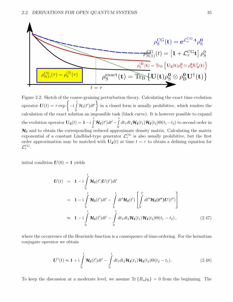
Figure 2.2: Sketch of the coarse-graining perturbation theory. Calculating the exact time evolution
operator U(t) = τ exp
−i
t∫0
HI(t′)dt′
in a closed form is usually prohibitive, which renders the
calculation of the exact solution an impossible task (black curve). It is however possible to expand
the evolution operator U2(t) = 1−it∫
0
HI(t′)dt′−
t∫0
dt1dt2HI(t1)HI(t2)Θ(t1−t2) to second order in
HI and to obtain the corresponding reduced approximate density matrix. Calculating the matrixexponential of a constant Lindblad-type generator LCG
τ is also usually prohibitive, but the firstorder approximation may be matched with U2(t) at time t = τ to obtain a defining equation forLCGτ .
initial condition U (0) = 1 yields
U (t) = 1− i
t∫0
HI(t′)U(t′)dt′
= 1− i
t∫0
HI(t′)dt′ −
t∫0
dt′HI(t′)
t′∫0
dt′′HI(t′′)U(t′′)
≈ 1− i
t∫0
HI(t′)dt′ −
t∫0
dt1dt2HI(t1)HI(t2)Θ(t1 − t2) , (2.47)
where the occurrence of the Heaviside function is a consequence of time-ordering. For the hermitianconjugate operator we obtain
U †(t) ≈ 1 + i
t∫0
HI(t′)dt′ −
t∫0
dt1dt2HI(t1)HI(t2)Θ(t2 − t1) . (2.48)
To keep the discussion at a moderate level, we assume Tr BαρB = 0 from the beginning. The
36 CHAPTER 2. OBTAINING A MASTER EQUATION
exact solution ρS(t) = TrB
U(t)ρ0
S ⊗ ρBU†(t)
is then approximated by
ρ(2)S (t) ≈ TrB
1− i
t∫0
HI(t1)dt1 −t∫
0
dt1dt2HI(t1)HI(t2)Θ(t1 − t2)
ρ0S ⊗ ρB ×
×
1 + i
t∫0
HI(t1)dt1 −t∫
0
dt1dt2HI(t1)HI(t2)Θ(t2 − t1)
= ρ0S + TrB
t∫
0
dt1
t∫0
dt2HI(t1)ρ0S ⊗ ρBHI(t2)
−
t∫0
dt1dt2TrB
Θ(t1 − t2)HI(t1)HI(t2)ρ0
S ⊗ ρB + Θ(t2 − t1)ρ0S ⊗ ρBHI(t1)HI(t2)
.
(2.49)
Again, we introduce the bath correlation functions with two time arguments as in Eq. (2.19)
Cαβ(t1, t2) = Tr Bα(t1)Bβ(t2)ρB , (2.50)
such that we have
ρ(2)S (t) = ρ0
S +∑αβ
t∫0
dt1
t∫0
dt2Cαβ(t1, t2)[Aβ(t2)ρ0
SAα(t1)
−Θ(t1 − t2)Aα(t1)Aβ(t2)ρ0S −Θ(t2 − t1)ρ0
SAα(t1)Aβ(t2)]. (2.51)
Typically, in the interaction picture, the system coupling operators Aα(t) will simply carry someoscillatory time dependence. In the worst case, they may remain time-independent. Therefore,the decay of the correlation function is essential for the convergence of the above integrals. Inparticular, we note that the truncated density matrix may remain finite even when t → ∞,rendering the expansion convergent also in the long-term limit.
Coarse-Graining
The basic idea of coarse-graining is to match this approximate expression for the system densitymatrix at time t = τ with one resulting from a Markovian generator
ρSCG(τ) = eL
CGτ ·τρ0
S ≈ ρ0S + τLCG
τ ρ0S , (2.52)
2.2. DERIVATIONS FOR OPEN QUANTUM SYSTEMS 37
such that we can infer the action of the generator on an arbitrary density matrix
LCGτ ρS =
1
τ
∑αβ
τ∫0
dt1
τ∫0
dt2Cαβ(t1, t2)[Aβ(t2)ρSAα(t1)
−Θ(t1 − t2)Aα(t1)Aβ(t2)ρS −Θ(t2 − t1)ρSAα(t1)Aβ(t2)]
= −i
1
2iτ
τ∫0
dt1
τ∫0
dt2∑αβ
Cαβ(t1, t2)sgn(t1 − t2)Aα(t1)Aβ(t2),ρS
+
1
τ
τ∫0
dt1
τ∫0
dt2∑αβ
Cαβ(t1, t2)
[Aβ(t2)ρSAα(t1)− 1
2Aα(t1)Aβ(t2),ρS
],(2.53)
where we have inserted Θ(x) = 12
[1 + sgn(x)] – in order to separate unitary and dissipative effectsof the system-reservoir interaction.
Box 9 (CG Master Equation) In the weak coupling limit, an interaction Hamiltonian of theform HI =
∑αAα ⊗Bα leads to the Lindblad-form master equation in the interaction picture
ρS = −i
1
2iτ
τ∫0
dt1
τ∫0
dt2∑αβ
Cαβ(t1, t2)sgn(t1 − t2)Aα(t1)Aβ(t2),ρS
+
1
τ
τ∫0
dt1
τ∫0
dt2∑αβ
Cαβ(t1, t2)
[Aβ(t2)ρSAα(t1)− 1
2Aα(t1)Aβ(t2),ρS
],
where the bath correlation functions are given by
Cαβ(tt, t2) = Tre+iHBt1Bαe
−iHBt1e+iHBt2Bβe−iHBt2 ρB
. (2.54)
We have not used hermiticity of the coupling operators nor that the bath correlation functionsdo typically only depend on a single argument. However, if the coupling operators were chosenhermitian, it is easy to show the Lindblad form. For completeness, we also note there that aLindblad form is also obtained for non-hermitian couplings. Obtaining the master equation requiresthe calculation of bath correlation functions and the evolution of the coupling operators in theinteraction picture.
Exercise 20 (Lindblad form) (1 point)By assuming hermitian coupling operators Aα = A†α, show that the CG master equation is ofLindblad form for all coarse-graining times τ .
38 CHAPTER 2. OBTAINING A MASTER EQUATION
Correspondence to the quantum-optical master equation
Let us make once more the time-dependence of the coupling operators explicit, which is mostconveniently done in the system energy eigenbasis. Now, we also assume that the bath correlationfunctions only depend on the difference of their time arguments Cαβ(t1, t2) = Cαβ(t1 − t2), suchthat we may use the Fourier transform definitions in Eq. (2.33) to obtain
ρS = −i
1
2iτ
∑abc
τ∫0
dt1
τ∫0
dt2∑αβ
Cαβ(t1 − t2)sgn(t1 − t2) |a〉 〈a|Aα(t1) |c〉 〈c|Aβ(t2) |b〉 〈b| ,ρS
+
1
τ
τ∫0
dt1
τ∫0
dt2∑αβ
∑abcd
Cαβ(t1 − t2)[|a〉 〈a|Aβ(t2) |b〉 〈b|ρS |d〉 〈d|Aα(t1) |c〉 〈c|
−1
2|d〉 〈d|Aα(t1) |c〉 〈c| · |a〉 〈a|Aβ(t2) |b〉 〈b| ,ρS
]= −i
1
4iπτ
∫dω∑abc
τ∫0
dt1
τ∫0
dt2∑αβ
σαβ(ω)e−iω(t1−t2)e+i(Ea−Ec)t1e+i(Ec−Eb)t2Acbβ Aacα [Lab,ρS]
+1
2πτ
∫dω
τ∫0
dt1
τ∫0
dt2∑αβ
∑abcd
γαβ(ω)e−iω(t1−t2)e+i(Ea−Eb)t2e+i(Ed−Ec)t1Aabβ Adcα ×
×[LabρSL
†cd −
1
2
L†cdLab,ρS
]. (2.55)
We perform the temporal integrations by invoking
τ∫0
eiαktkdtk = τeiαkτ/2sinc[αkτ
2
](2.56)
with sinc(x) = sin(x)/x to obtain
ρS = −iτ
4iπ
∫dω∑abc
∑αβ
σαβ(ω)eiτ(Ea−Eb)/2sinc[τ
2(Ea − Ec − ω)
]sinc
[τ2
(Ec − Eb + ω)]×
×〈c|Aβ |b〉 〈c|A†α |a〉∗ [|a〉 〈b| ,ρS]
+τ
2π
∫dω∑αβ
∑abcd
γαβ(ω)eiτ(Ea−Eb+Ed−Ec)/2sinc[τ
2(Ed − Ec − ω)
]sinc
[τ2
(ω + Ea − Eb)]×
×〈a|Aβ |b〉 〈c|A†α |d〉∗[|a〉 〈b|ρS (|c〉 〈d|)† − 1
2
(|c〉 〈d|)† |a〉 〈b| ,ρS
]. (2.57)
Therefore, we have the same structure as before, but now with coarse-graining time dependentdampening coefficients
ρS = −i
[∑ab
στab |a〉 〈b| ,ρS
]
+∑abcd
γτab,cd
[|a〉 〈b|ρS (|c〉 〈d|)† − 1
2
(|c〉 〈d|)† |a〉 〈b| ,ρS
](2.58)
2.2. DERIVATIONS FOR OPEN QUANTUM SYSTEMS 39
with the coefficients
στab =1
2i
∫dω∑c
eiτ(Ea−Eb)/2 τ
2πsinc
[τ2
(Ea − Ec − ω)]
sinc[τ
2(Eb − Ec − ω)
]×
×
[∑αβ
σαβ(ω) 〈c|Aβ |b〉 〈c|A†α |a〉∗
],
γτab,cd =
∫dωeiτ(Ea−Eb+Ed−Ec)/2 τ
2πsinc
[τ2
(Ed − Ec − ω)]
sinc[τ
2(Eb − Ea − ω)
]×
×
[∑αβ
γαβ(ω) 〈a|Aβ |b〉 〈c|A†α |d〉∗
]. (2.59)
Finally, we note that in the limit of large coarse-graining times τ → ∞ and assuming hermitiancoupling operators Aα = A†α, these dampening coefficients converge to the ones in definition 8, i.e.,formally
limτ→∞
στab = σab ,
limτ→∞
γτab,cd = γab,cd . (2.60)
Exercise 21 (CG-BMS correspondence) (1 points)Show for hermitian coupling operators that when τ →∞, CG and BMS approximation are equiv-alent. You may use the identity
limτ→∞
τsinc[τ
2(Ωa − ω)
]sinc
[τ2
(Ωb − ω)]
= 2πδΩa,Ωbδ(Ωa − ω) .
This shows that coarse-graining provides an alternative derivation of the quantum-optical mas-ter equation, replacing three subsequent approximations (Born-, Markov- and secular) by just one(perturbative expansion in the interaction).
2.2.3 Thermalization
The BMS limit has beyond its relatively compact Lindblad form further appealing properties inthe case of a bath that is in thermal equilibrium
ρB =e−βHB
Tr e−βHB(2.61)
with inverse temperature β. These root in further analytic properties of the bath correlationfunctions such as the Kubo-Martin-Schwinger (KMS) condition
Cαβ(τ) = Cβα(−τ − iβ) . (2.62)
Exercise 22 (KMS condition) (1 points)
Show the validity of the KMS condition for a thermal bath with ρB = e−βHB
Tre−βHB .
40 CHAPTER 2. OBTAINING A MASTER EQUATION
For the Fourier transform, this shift property implies
γαβ(−ω) =
+∞∫−∞
Cαβ(τ)e−iωτdτ =
+∞∫−∞
Cβα(−τ − iβ)e−iωτdτ
=
−∞−iβ∫+∞−iβ
Cβα(τ ′)e+iω(τ ′+iβ)(−)dτ ′ =
+∞−iβ∫−∞−iβ
Cβα(τ ′)e+iωτ ′dτ ′e−βω
=
+∞∫−∞
Cβα(τ ′)e+iωτ ′dτ ′e−βω = γβα(+ω)e−βω , (2.63)
where in the last line we have used that the bath correlation functions are analytic in τ in the com-plex plane and vanish at infinity, such that we may safely deform the integration contour. Finally,the KMS condition can thereby be used to prove that for a reservoir with inverse temperature β,the density matrix
ρS =e−βHS
Tr e−βHS(2.64)
is one stationary state of the BMS master equation (and the τ →∞ limit of the CG appraoch).
Exercise 23 (Thermalization) (1 points)
Show that ρS = e−βHS
Tre−βHS is a stationary state of the BMS master equation, when γαβ(−ω) =
γβα(+ω)e−βω.
When the reservoir is in the grand-canonical equilibrium state
ρB =e−β(HB−µNB)
Tr e−β(HB−µNB), (2.65)
where N = NS + NBis a conserved quantity [HS +HB +HI, NS +NB] = 0, the KMS condition isnot fulfilled anymore. However, even in this case one can show that a stationary state of the BMSmaster equation is given by
ρS =e−β(HS−µNS)
Tr e−β(HS−µNS), (2.66)
i.e., both temperature β and chemical potential µ equilibrate.
2.2.4 Example: Spin-Boson Model
The spin-boson model describes the interaction of a spin with a bosonic environment
HS = Ωσz + Tσx , HB =∑k
ωkb†kbk ,
HI = σz ⊗∑k
[hkbk + h∗kb
†k
], (2.67)
2.2. DERIVATIONS FOR OPEN QUANTUM SYSTEMS 41
where Ω and T denote parameters of the system Hamiltonian, σα the Pauli matrices, and b† createsa boson with frequency ωk in the reservoir. The model can be motivated by a variety of setups,e.g. a charge qubit (singly-charged double quantum dot) that is coupled to vibrations. We notethe a priori hermitian coupling operators
A1 = σz , B1 =∑k
[hkbk + h∗kb
†k
]. (2.68)
We first diagonalize the system part of the Hamiltonian to obtain the eigenbasisHS |n〉 = En |n〉,where
E± = ±√
Ω2 + T 2 , |±〉 =1√
T 2 +(Ω±√
Ω2 + T 2)2
[(Ω±√
Ω2 + T 2)|0〉+ T |1〉
], (2.69)
where |0/1〉 denote the eigenvectors of the σz Pauli matrix with σz |i〉 = (−1)i |i〉.
Exercise 24 (Eigenbasis) (1 points)Confirm the validity of Eq. (2.69).
Second, we calculate the correlation function (in this case, there is just one). Transformingeverything in the interaction picture we see that the annihilation operators just pick up time-dependent phases
C(τ) = Tr
∑k
[hkbke
−iωkτ + h∗kb†ke
+iωkτ]∑
q
[hqbq + h∗qb
†q
]ρB
=
∑k
|hk|2[e−iωkτ (1 + nB(ωk)) + e+iωkτnB(ωk)
]=
1
2π
∫dωΓ(ω)
[e−iωτ (1 + nB(ω)) + e+iωτnB(ω)
], (2.70)
where we have introduced the spectral coupling density Γ(ω) = 2π∑
k |hk|2δ(ω−ωk) and the Bose
distribution
nB(ω) =1
eβ(ω−µ) − 1. (2.71)
Exercise 25 (Bose distribution) (1 points)Confirm the validity of Eq. (2.71), i.e., show that
δkqnB(ωk) = Tr
b†kbq
e−β(HB−µNB)
Z
, (2.72)
where HB =∑
k ωkb†kbk, NB =
∑k b†kbk, and Z = Tr
e−β(HB−µNB)
.
42 CHAPTER 2. OBTAINING A MASTER EQUATION
We can directly read off the even Fourier transform of the correlation function
γ(ω) = Γ(+ω)Θ(+ω)[1 + nB(+ω)] + Γ(−ω)Θ(−ω)nB(−ω) . (2.73)
We note that for bosons we necessarily have Γ(ω < 0) = 0, since all oscillator frequencies in thereservoir must be positive. We compute some relevant dampening coefficients
γ−+,−+ = Γ(+2√
Ω2 + T 2)[1 + nB(+2√
Ω2 + T 2)]|〈−|σz |+〉|2 ,γ+−,+− = Γ(+2
√Ω2 + T 2)nB(+2
√Ω2 + T 2)|〈−|σz |+〉|2 ,
γ−−,++ = γ(0) 〈−|σz |−〉 〈+|σz |+〉 . (2.74)
The explicit calculation of the non-vanishing Lamb-shift terms σ−− and σ++ is possible but moreinvolved. Fortunately, it can be omitted for many applications. Since the system Hamiltonian isnon-degenerate, the populations evolve according to
ρ−− = +γ−+,−+ρ++ − γ+−,+−ρ−− , ρ++ = +γ+−,+−ρ−− − γ−+,−+ρ++ , (2.75)
which is independent from the coherences
ρ−+ = −i (E− − E+ + σ−− − σ++) ρ−+ +
[γ−−,++ −
γ−+,−+ + γ+−,+−
2
]ρ−+ . (2.76)
Since the Lamb-shift terms σii are purely imaginary, the quantities at hand already allow us to
deduce that the coherences will decay |ρ−+|2 = e−(−2γ−−,+++γ−+,−++γ+−,+−)t∣∣ρ0−+
∣∣2, which showsthat the decoherence rate increases with temperature (finite nB) but can also at zero temperaturenot be suppressed below a minimum value. A special (exactly solvable) case arises when T = 0:Then, the interaction commutes with the system Hamiltonian leaving the energy of the systeminvariant. Consistently, the eigenbasis is in this case that of σz and the coefficients γ−+,−+ andγ+−,+− do vanish. In contrast, the coefficient γ−−,++ → −γ(0) may remain finite. Such modelsare called pure dephasing models (since only their coherences decay). However, for finite T thesteady state of the master equation is given by (we assume here µ = 0)
ρ++
ρ−−=γ+−,+−
γ−+,−+
=nB(+2
√Ω2 + T 2)
1 + nB(+2√
Ω2 + T 2)= e−2β
√Ω2+T 2
, (2.77)
i.e., the stationary state is given by the thermalized one.
Chapter 3
Multi-Terminal Coupling :Non-Equilibrium Case I
The most obvious way to achieve non-equilibrium dynamics is to use reservoir states that are non-thermalized, i.e., states that cannot simply be characterized by just temperature and chemicalpotential. Since the derivation of the master equation only requires [ρB,HB] = 0, this would stillallow for many nontrivial models, 〈n| ρB |n〉 could e.g. follow multi-modal distributions. Alterna-tively, a non-equilibrium situation may be established when a system is coupled to different thermalequilibrium baths or of course when the system itself is externally driven – either unconditionally(open-loop feedback) or conditioned on the actual state of the system (closed-loop feedback).
First, we will consider the case of multiple reservoirs at different thermal equilibria that are onlyindirectly coupled via the system: Without the system, they would be completely independent.Since these are chosen at different equilibria, they drag the system towards different thermal states,and the resulting stationary state is in general a non-thermal one. Since the different compartmentsinteract only indirectly via the system, we have the case of a multi-terminal system, where one canmost easily derive the corresponding master equation, since each contact may be treated separately.Therefore, we do now consider multiple (K) reservoirs
HB =K∑`=1
H(`)B (3.1)
with commuting individual parts[H(`)
B ,H(k)B
]= 0. These are held at different chemical potentials
and different temperatures
ρB =e−β(H(1)
B −µN(1)B )
Tre−β(H(1)
B −µN(1)B ) ⊗ . . .⊗ e−β(H(K)
B −µN(K)B )
Tre−β(H(K)
B −µN(K)B ) . (3.2)
To each of the reservoirs, the system is coupled via different coupling operators
HI =∑α
Aα ⊗k∑`=1
B(`)α . (3.3)
Since we assume that the first order bath correlation functions vanish⟨B`αρB
⟩= 0, the second-order
bath correlation functions may be computed additively
Cαβ(τ) =K∑`=1
C(`)αβ(τ) . (3.4)
43
44 CHAPTER 3. MULTI-TERMINAL COUPLING : NON-EQUILIBRIUM CASE I
Exercise 26 (Additive Reservoirs) (1 points)Show with using Eqns. (3.1) and (3.2) that expectation values of coupling operators belonging todifferent reservoirs vanish, i.e.,
C(α,`),(β,k)(τ) = TrB(`)α (τ)B
(k)β ρB
= δk`C(α,`),(β,`) .
This obviously transfers to their Fourier transforms and thus, also to the final Liouvillian (tosecond order in the coupling)
L = L(0) +K∑`=1
L(`) . (3.5)
Here, L(0)ρ= − i [HS, ρ] describes the action of the system Hamiltonian and L(`) denotes the Li-ouvillian resulting only from the `-th reservoir. The resulting stationary state is in general anon-equilibrium one.
Let us however first identify a special case where even in a non-equilibrium setup we candetermine the non-equilibrium steady state analytically. For some simple models, one obtains thatthe coupling structure of all Liouvillians is identical for different reservoirs
L(`) = Γ(`)[LA + n(`)LB
], (3.6)
i.e., the reservoirs trigger exactly the same transitions within the system. Here, n(`) is a parameterencoding the thermal properties of the respective bath (e.g. a Fermi-Dirac or a Bose-Einsteindistribution evaluated at one of the systems transition frequencies), and LA/B simply label partsof the Liouvillian that are proportional to thermal characteristics (B) or not (A). Finally, Γ(`)
represent coupling constants to the different reservoirs. For coupling to a single reservoir, thestationary state is defined via the equation
L(`)ρ(`) = Γ(`)[LA + n(`)LB
]ρ(`) = 0 (3.7)
and thus implicitly depends on the thermal parameter ρ(`) = ρ(n(`)). Obviously, the steady statewill be independent of the coupling strength Γ(`). For the total Liouvillian, it follows that thedependence of the full stationary state on all thermal parameters simply given by the same depen-dence on an average thermal parameter
Lρ =∑`
L(`)ρ =∑`
Γ(`)[LA + n(`)LB
]ρ =
[∑`
Γ(`)
][LA +
∑` Γ(`)n(`)∑`′ Γ
(`′)LB]ρ ,
=
[∑`
Γ(`)
][LA + nLB] ρ , (3.8)
where
n =
∑` Γ(`)n(`)∑` Γ(`)
(3.9)
3.1. CONDITIONAL MASTER EQUATION FROM CONSERVATION LAWS 45
represents an average thermal parameter (e.g. the average occupation). Formally, this is thesame equation that determines the steady state for a single reservoir, which may now however benon-thermal.
This can be illustrated by upgrading the Liouvillian for a single resonant level coupled to asingle junction
L =
(−Γf +Γ(1− f)+Γf −Γ(1− f)
), (3.10)
where the Fermi function f =[eβ(ε−µ) + 1
]−1of the contact is evaluated at the dot level ε, to the
Liouvillian for a single-electron transistor (SET) coupled to two (left and right) junctions
L =
(−ΓLfL − ΓRfR +ΓL(1− fL) + ΓR(1− fR)+ΓLfL + ΓRfR −ΓL(1− fL)− ΓR(1− fR)
). (3.11)
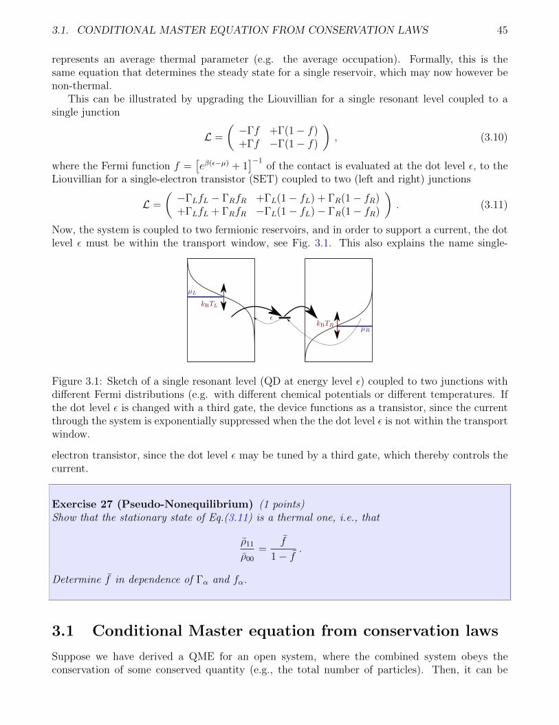
Now, the system is coupled to two fermionic reservoirs, and in order to support a current, the dotlevel ε must be within the transport window, see Fig. 3.1. This also explains the name single-
Figure 3.1: Sketch of a single resonant level (QD at energy level ε) coupled to two junctions withdifferent Fermi distributions (e.g. with different chemical potentials or different temperatures. Ifthe dot level ε is changed with a third gate, the device functions as a transistor, since the currentthrough the system is exponentially suppressed when the the dot level ε is not within the transportwindow.
electron transistor, since the dot level ε may be tuned by a third gate, which thereby controls thecurrent.
Exercise 27 (Pseudo-Nonequilibrium) (1 points)Show that the stationary state of Eq.(3.11) is a thermal one, i.e., that
ρ11
ρ00
=f
1− f.
Determine f in dependence of Γα and fα.
3.1 Conditional Master equation from conservation laws
Suppose we have derived a QME for an open system, where the combined system obeys theconservation of some conserved quantity (e.g., the total number of particles). Then, it can be
46 CHAPTER 3. MULTI-TERMINAL COUPLING : NON-EQUILIBRIUM CASE I
directly concluded that a change in the system particle number by e.g. minus one must be directlyaccompagnied by the corresponding change of the reservoir particle number by plus one. Forcouplings to multiple reservoirs these terms can also be uniquely identified, since the Liouvilliansare additive. Whereas its actual density matrix says little about the number of quanta that havealready passed the quantum system, a full trajectory would reveal this information. In such cases,it is reasonable to discretize the master equation in time, where it can most easily be upgraded toan n-resolved (conditional) master equation. In what follows, we just track the particle number ina single attached reservoir and denote by ρ(n)(t) the system density matrix under the condition thatn net particles have left into the monitored reservoirs, but the method may easily be generalized.Assuming that at time t, we have n particles transferred to the reservoir, we may discretize theconventional master equation ρ = Lρ in time and identify terms that increase or decrease theparticle number (often called jumpers)
ρ(n) = L0ρ(n) + L+ρ
(n−1) + L−ρ(n+1) . (3.12)
Here, L+ increases the number of particles in the monitored reservoirs by one and L− decreasesit by one. All remaining processes (jumps to other reservoirs or internal transitions within thesystem) are contained in L0, such that the original Liouvillian is given by
L = L0 + L− + L+ . (3.13)
Since the total number of transferred particles is normally not constrained, this immediately yieldsan infinite set of equations for the conditioned system density matrix. Exploiting the translationalinvariance suggests to use the (discrete) Fourier transform
ρ(χ, t) =∑n
ρ(n)(t)e+inχ , (3.14)
which recovers the original dimension of the master equation
ρ(χ, t) =[L0 + e+iχL+ + e−iχL−
]ρ(χ, t) = L(χ)ρ(χ, t) , (3.15)
but at the cost of introducing the parameter χ – called counting field further-on.
Exercise 28 (Counting Field Master Equation) (1 points)How would Eqns. (3.12) and (3.15) change when particles could only tunnel in pairs?
The advantage of this form however is that – since χ is a parameter – we can readily writedown the solution
ρ(χ, t) = eL(χ)tρ(χ, 0) = eL(χ)tρ0 , (3.16)
where we have used the convention that ρ(n)(0) = δn,0ρ0. We stress here again that we have writteneverything in superoperator notation, i.e., the density matrix elements are arranged in a vector(conventionally, one puts the populations first), such that the Liouvillian acts as a matrix fromthe left. Stating that the populations evolve independently from the coherences corresponds toa block form of the Liouvillian in this picture. Having solved the master equation for ρ(t), we
3.1. CONDITIONAL MASTER EQUATION FROM CONSERVATION LAWS 47
can then rearrange the solution vector into matrix form and calculate traces with operators etc.However, noticing that we can of course also represent ordinary operators acting in the Hilbertspace of the system as superoperators, it is important to realize that we can conveniently performall operations in superoperator notation. Since the trace just involves summing over the diagonalelements of the result, this transfers to a product with a transposed vector of the form (we takean N ×N density matrix)
Tr Aρ =Tr Aρ =
1, . . . , 1︸ ︷︷ ︸N
, 0, . . . , 0
(A)
ρ11...
ρNNρ12...
ρN,N−1
. (3.17)
Exercise 29 (Superoperators) How would the Pauli matrix σx act on the density matrix if itwas arranged as a superoperator, i.e., determine Σx and Σx in
(0 11 0
)(ρ00 ρ01
ρ10 ρ11
)= Σx
ρ00
ρ11
ρ01
ρ10
,
(ρ00 ρ01
ρ10 ρ11
)(0 11 0
)= Σx
ρ00
ρ11
ρ01
ρ10
. (3.18)
As an example, we phenomenologically convert the SET master equation (3.11) into an n-resolved version. Since we have a simple rate equation, we have neglected the block describingthe evolution of coherences. We choose the right reservoir as the one to monitor and denote thenumber of particles that have tunneled into the right reservoir by n, where negative n would simplyimply a current from right to left. Then, the conditional density matrix obeys
ρ(n) =
(−ΓLfL − ΓRfR +ΓL(1− fL)
+ΓLfL −ΓL(1− fL)− ΓR(1− fR)
)ρ(n)
+
(0 ΓR(1− fR)0 0
)ρ(n−1) +
(0 0
+ΓRfR 0
)ρ(n+1) . (3.19)
Performing the Fourier transformation (thereby exploiting the shift invariance) reduces the dimen-sion at the price of introducing the counting field
ρ(χ, t) =
(−ΓLfL − ΓRfR +ΓL(1− fL) + ΓR(1− fR)e+iχ
+ΓLfL + ΓRfRe−iχ −ΓL(1− fL)− ΓR(1− fR)
)ρ(χ, t) . (3.20)
Formally, this just corresponds to the replacement (1 − fR) → (1 − fR)e+iχ and fR → fRe−iχ in
the off-diagonal matrix elements of the Liouvillian (which correspond to particle jumps).
48 CHAPTER 3. MULTI-TERMINAL COUPLING : NON-EQUILIBRIUM CASE I
The original density matrix can be recovered by summing over all conditioned density matrices
ρ(t) =∑n
ρ(n)(t) , (3.21)
which also shows that the conditioned ones need not be normalized. We can obtain the informationabout the tunneled particles by tracing over the system degrees of freedom
Pn(t) = Trρ(n)(t)
. (3.22)
Unfortunately, obtaining ρ(n)(t) would require to solve an infinite-dimensional system, such thatthis is usually not a very practical way.
3.2 Microscopic derivation with virtual detectors
Unfortunately, we do not always have a conserved quantity that may only change when tunnelingacross the system-reservoir junction takes place. A counter-example may be the tunneling betweentwo reservoirs, that is merely modified by the presence of the quantum system (e.g. quantum pointcontact monitoring a charge qubit) and is not connected with a particle change in the system. Insuch cases, we may not identify a change in the system state with a microcanonical change of thereservoir state. However, such problems can still be handled with a quantum master equation byintroducing a virtual detector at the level of the interaction Hamiltonian. Suppose that in theinteraction Hamiltonian we can identify terms associated with a change of the tracked obervablein the reservoir
HI = A+ ⊗B+ + A− ⊗B− +∑
α 6=+,−
Aα ⊗Bα , (3.23)
where B+ increases and B− decreases the reservoir particle number. We extend the system Hilbertspace by adding a virtual detector
HS → HS ⊗ 1 , HB → HB
HI → +[A+ ⊗D†
]⊗B+ + [A− ⊗D]⊗B− +
∑α 6=+,−
[Aα ⊗ 1]⊗Bα , (3.24)
where D =∑
n |n〉 〈n+ 1| and D† =∑
n |n+ 1〉 〈n|. Here |n〉 are the eigenstates of the detector,and we see that D† |n〉 = |n+ 1〉 and D |n〉 = |n− 1〉. This obviously also implies that DD† =D†D = 1. Such a detector is ideal in the sense that it does not influence the system dynamicsand it does not have its own energy content (its own Hamiltonian vanishes). Therefore, it will becalled virtual detector here. The detector operators in the interaction Hamiltonian can also beviewed as bookkeeping operators that simply facilitate the correct identification of terms in themaster equation. We can now formally consider the detector as part of the system and derive themaster equation. Since there is no direct interaction between the original system and the detector,the eigenbasis of both system and detector is now given by |a, n〉 = |a〉 ⊗ |n〉, and we may derivee.g. the coarse-graining master equation in the usual way. When we decompose the system densitymatrix as
ρ(t) =∑n
ρ(n)(t)⊗ |n〉 〈n| , (3.25)
3.3. FULL COUNTING STATISTICS 49
we see that we can reduce the Lindblad master equation by using that
〈n|DA−ρA+D† |n〉 = A−ρ
(n+1)A+ ,
〈n|D†A+ρA−D |n〉 = A+ρ(n−1)A− (3.26)
to a form like in Eq. (3.12). The coarse-graining master equation in Box 9 for example shows thatsuch conditioned master equations can be readily derived.
3.3 Full Counting Statistics
To obtain the probability of having n tunneled particles into a respective reservoir, we have to sumover the different system configurations of the corresponding conditional density matrix
Pn(t) = Trρ(n)(t)
. (3.27)
In view of the identities
Tr ρ(χ, t) = TreL(χ)tρ0
=∑n
Pn(t)e+inχ , (3.28)
we see that in order to evaluate moments⟨nk⟩, we simply have to take derivatives with respect to
the counting field
⟨nk(t)
⟩=∑n
nkPn(t) = (−i∂χ)k∑n
Pn(t)e+inχ
∣∣∣∣∣χ=0
. (3.29)
Based on a conditional master equation, this enables a very convenient calculation of the stationarycurrent. This is a good motivation to introduce the moment-generating function.
Box 10 (Moment-Generating Function) The moment-generating function is given by
M(χ, t) = TreL(χ)tρ0
, (3.30)
and moments can be computed from derivatives with respect to the counting field⟨nk(t)
⟩= (−i∂χ)kM(χ, t)
∣∣χ=0
. (3.31)
Often, the initial condition is set to the steady-state solution ρ0 = ρ with L(0)ρ = 0.
Taking the stationary density matrix L(0)ρ = 0 as initial condition (the stationary current isindependent on the initial occupation of the density matrix), we obtain for the current as the time
50 CHAPTER 3. MULTI-TERMINAL COUPLING : NON-EQUILIBRIUM CASE I
derivative of the first moment
I = 〈n(t)〉
= −i∂χd
dtTreL(χ)tρ
∣∣χ=0
= −i∂χ TrL(χ)eL(χ)tρ
∣∣χ=0
= −iTrL′(0)ρ+ [L′(0)L(0) + L(0)L′(0)] tρ
+[L′(0)L2(0) + L(0)L′(0)L(0) + L2(0)L′(0)
] t22ρ+ . . .
= −iTr L′(0)ρ , (3.32)
where we have used L(0)ρ = 0 and also Tr L(0)σ = 0 for all operators σ (trace conservation).This is consistent with common definitions of a current entering or leaving the system, since e.g.for sequential tunneling we have
I = −iTr L′(0)ρ = Tr [L+ − L−] ρ . (3.33)
Formally, we see that a stationary occupation times a transition rate yields a current. Morequantitatively, by our initial definition, L+ contained the rates responsible for particles leaving thesystem towards the monitored reservoir whereas L− described the inverse process.
Exercise 30 (Stationary SET current) (1 points)Calculate the stationary current through the SET (3.20).
Sometimes a description in terms of cumulants is more convenient.
Box 11 (Cumulant-Generating Function) The cumulant-generating function is defined as thelogarithm of the moment-generating function
C(χ, t) = lnM(χ, t) = ln TreL(χ)tρ0
, (3.34)
and all cumulants may be obtained via simple differentiation⟨⟨nk⟩⟩
= (−i∂χ)k C(χ, t)|χ=0 . (3.35)
Cumulants and Moments are of course related, we just summarize relations for the lowest fewcumulants
〈〈n〉〉 = 〈n〉 ,⟨⟨n2⟩⟩
=⟨n2⟩− 〈n〉2 ,⟨⟨
n3⟩⟩
=⟨n3⟩− 3 〈n〉
⟨n2⟩
+ 2 〈n〉3 ,⟨⟨n4⟩⟩
=⟨n4⟩− 4 〈n〉
⟨n3⟩− 3
⟨n2⟩2
+ 12 〈n〉2⟨n2⟩− 6 〈n〉4 . (3.36)
3.4. CUMULANT-GENERATING FUNCTION 51
Obviously, the first two cumulants are just the mean and width of the probability distribution. Forunimodal distributions, the third cumulant (skewness) and the fourth cumulant (kurtosis) describethe shape of the distribution near its maximum. In contrast to moments, higher cumulants areinert when a trivial transformation such as a simple shift is performed on a probability distribution.
3.4 Cumulant-Generating Function
The clear advantage of the description by cumulants however lies in the fact that the long-termevolution of the cumulant-generating function is usually given by the dominant eigenvalue of theLiouvillian
C(χ, t) ≈ λ(χ)t , (3.37)
where λ(χ) is the (uniqueness assumed) eigenvalue of the Liouvillian that vanishes at zero countingfield λ(0) = 0. For this reason, the dominant eigenvalue is also interpreted as the cumulant-generating function of the stationary current.
Exercise 31 (current CGF for the SET) (1 points)Calculate the dominant eigenvalue of the SET Liouvillian (3.20) in the infinite bias limit fL → 1and fR → 0. What is the value of the current?
We show this by using the decomposition of the Liouvillian in Jordan Block form
L(χ) = Q(χ)LJ(χ)Q−1(χ) , (3.38)
where Q(χ) is a (non-unitary) similarity matrix and LJ(χ) contains the eigenvalues of the Liouvil-lian on its diagonal – distributed in blocks with a size corresponding to the eigenvalue multiplicity.We assume that there exists one stationary state ρ, i.e., one eigenvalue λ(χ) with λ(0) = 0 and thatall other eigenvalues have a larger negative real part near χ = 0. Then, we use this decompositionin the matrix exponential to estimate its long-term evolution
M(χ, t) = TreL(χ)tρ0
= Tr
eQ(χ)LJ (χ)Q−1(χ)tρ0
= Tr
Q(χ)eLJ (χ)tQ−1(χ)ρ0
→ Tr
Q(χ)
eλ(χ)·t
0. . .
0
Q−1(χ)ρ0
= eλ(χ)·tTr
Q(χ)
1
0. . .
0
Q−1(χ)ρ0
= eλ(χ)tc(χ) (3.39)
with some polynomial c(χ) depending on the matrix Q(χ). This implies that the cumulant-generating function
C(χ, t) = lnM(χ, t) = λ(χ)t+ ln c(χ) ≈ λ(χ)t (3.40)
becomes linear in λ(χ) for large times.
52 CHAPTER 3. MULTI-TERMINAL COUPLING : NON-EQUILIBRIUM CASE I
3.5 Energetic Counting
With a similiar theoretical apparatus, it is also possible to count the energetic exchanges betweenthe system and a monitored reservoir. Most systems that are described by a Markovian masterequation will only allow for discrete changes of their internal energy. If there is only a finite numberof allowed energetic transitions, we may also count the number of such transitions individually,similiar to the number of particles. For many transitions, this would induce many counting fields,but the total energy could be recovered from E =
∑i ωini, such that
P (E, t) =∑
n1,...,nk
Pn1,...,nk(t)δ(E −∑i
ωini) . (3.41)
would yield the probability of energy transfer E at time t. The most evident difference to particlecounting statistics is that while most Markovian models only allow for the exchange of singleparticles at a time (a consequence of the usual weak-coupling assumptions), there may be differentenergy quanta ω > 0 exchanged with the reservoirs
ρ(E) = L0ρ(E) +
∑ω
[L+ωρ
(E−ω) + L−ωρ(E+ω)]. (3.42)
Here, L+ω describes processes triggered by the monitored reservoir that increase the system energyby +ω whereas L−ω decrease the energy by the same amount. Consequently, the summation overω involves all allowed transitions within the system. Finally, L0 contains all remaining terms, suchthat L = L0 +
∑ω [L+ω + L−ω] holds. A second difference to particle counting is that – for more
than a single transition frequency ω – the total transferred energy may become continuous. Wetherefore perform a continuous Fourier transform
ρ(ξ, t) =
∫ρ(E)(t)e+iEξdE , (3.43)
which transforms the master equation into
ρ(ξ, t) = L0 +∑ω
[L+ωe
+iξω + L−ωe−iξω]ρ(ξ, t) = L(ξ)ρ(ξ, t) . (3.44)
Apart from the fact that the counting field ξ has dimension of inverse energy (the counting field ξwas dimensionless), all techniques from the particle counting statistics may be applied to energycounting statistics as well.
As a simple phenomenologic example, we consider a three-state system with unidirectionaltransport. The system can be empty |0〉 without carrying any energy E0 = 0, it can be occupiedin its left state |L〉 with energy εL and occupied in its right state |R〉 with energy εR. The ratematrix is in this basis given by
L =
−ΓL 0 +ΓR+ΓL −T 0
0 +T −ΓR
, (3.45)
demonstrating that the system can only be loaded from the left (+ΓL) and unload to the right(+ΓR), such that transport is uni-directional. Introducing counting fields for particle (χ) andenergy (ξ) transport into the right reservoir, the counting-field-dependent Liouvillian becomes
L(χ, ξ) =
−ΓL 0 +ΓRe+iχ+iξεR
+ΓL −T 00 +T −ΓR
, (3.46)
3.6. ENTROPY BALANCE 53
and the normalized steady state solution is given by
ρ =1
ΓLΓR + (ΓL + ΓR)T
ΓRTΓLΓRΓLT
. (3.47)
Therefore, we obtain for the matter current
IM = (1, 1, 1)
0 0 +ΓR0 0 00 0 0
ρ =ΓLΓRT
(ΓL + ΓR)T + ΓLΓR. (3.48)
Similiarly, the energy current becomes
IE = εRIM . (3.49)
Naturally, we observe that these currents vanish when either ΓL, ΓR, or T vanish.
Exercise 32 (Counting Terminal) (1 points)Introduce counting fields for energy and matter for the rate equation (3.45) when the left reservoiris monitored and compute both currents.
3.6 Entropy Balance
We now turn our focus to the central quantity in thermodynamics, the entropy. We assume that thedynamics of our system is described by a time-independent quantum master equation of Lindbladform. We can even allow for the possibility that the Lindblad generator L(t) is explicitly time-dependent due to an external driving (the approximations during the derivation in the previouschapters imply that then this driving must be very slow). Furthermore, we assume that it can beadditively decomposed in the number of reservoirs ν to which the system is coupled (this oftenarises in weak-coupling scenarios, but note that counter-examples exist)
ρ = L(t)ρ(t) = L(0)(t)ρ(t) +∑ν
L(ν)(t)ρ(t) . (3.50)
Here, L(0)(t)ρ(t)= − i [HS(t), ρ(t)] describes the action of a possibly driven system Hamiltonianonly. We assume that the time-dependent dissipator L(ν)(t) (which may e.g. also include theeffects of Lamb-shift) obeys some detailed balance relations leading to
L(ν)(t)ρ(ν)eq (t) = 0 , (3.51)
where we have introduced the time-dependent grand-canonical equilibrium state
ρ(ν)eq (t) =
e−βν [HS(t)−µνNS]
Zν(t)(3.52)
with inverse temperature βν , chemical potential µν , system Hamiltonian HS(t) and system par-ticle number operator NS. Apart from the time-dependence, these conditions are fulfilled by thequantum-optical Lindblad master equation.
54 CHAPTER 3. MULTI-TERMINAL COUPLING : NON-EQUILIBRIUM CASE I
3.6.1 Definitions
When we consider the change of the system energy under Lindblad dynamics, we see that it canbe decomposed as
E =d
dtTr HS(t)ρ(t)
= TrHSρ
+∑ν
µνTrNSL(ν)ρ
+∑ν
Tr
(HS(t)− µνNS)L(ν)ρ
= Wdrv + Wchem +∑ν
Q(ν) , (3.53)
where
Wdrv = TrHSρ
(3.54)
is the mechanical work performed on the system due to the external driving,
Wchem =∑ν
µνTrNSL(ν)ρ
(3.55)
is the chemical work performed on the system due to the flux of particles from reservoirs ν, andfinally
Q(ν) = Tr
(HS(t)− µνNS)L(ν)ρ, (3.56)
is the heat entering the system from reservoir ν. We note that at steady state and without drivingwe obtain the usual decomposition into energy and matter currents
Q(ν) = Tr
(HS − µνNS)L(ν)ρ
= I(ν)E − µνI
(ν)M . (3.57)
Opposed to our previous convention (counting currents entering the reservoir ν positively), here acurrent counts positive when it enters the system. That is, we have simply changed the pespective,which is unproblematic for currents. We can convince ourselves that e.g. for our the SET modelwithout coherences we have for the energy current entering the system from the left
I(L)E = (1, 1)
(0 00 ε
)(−ΓLfL +ΓL(1− fL)+ΓLfL −ΓL(1− fL)
)(1− ff
)= (1, 1)
(0 0
+εΓLfL −εΓL(1− fL)
)(1− ff
)= (1, 1)
(+εΓLfL(1− f)−εΓL(1− fL)f
)= εΓL(fL − f)
=εΓLΓR(fL − fR)
ΓL + ΓR, (3.58)
which is precisely what we had before for the energy current leaving towards the right terminal,i.e., at steady state the currents are conserved, and the first law of thermodynamics is obeyed.The calculation for the matter current is similar I
(L)E = εI
(L)M and it is of course also conserved.
These energy and matter currents will affect the dynamics of the entropy of the system, whichcan be quantified by the von-Neumann entropy.

3.6. ENTROPY BALANCE 55
Box 12 (von-Neumann entropy) The von-Neumann entropy of a quantum system describedby the density matrix ρ is given by
S[ρ] = −Tr ρ ln ρ , (3.59)
where ρ ln ρ is defined by the power series expansion.
The von-Neumann entropy can alternatively be obtained from the eigenvalues Pi of the densitymatrix
S[ρ] = −Tr
(UρDU†) ln(UρDU
†)
= −TrU(ρD ln ρD)U †
= −Tr ρD ln ρD = −
∑i
Pi lnPi .(3.60)
It vanishes for a pure state S[|Ψ〉 〈Ψ|] = 0 and is upper bounded by the dimension of the systemHilbert space N
S[ρ] ≤ lnN . (3.61)
This upper bound is directly found in the diagonal representation. Since the probabilities Pi haveto obey the normalization condition
∑Ni=1 Pi = 1 we use the method of Lagrange multipliers and
maximize S[ρ] = S[ρ] + λ(1−∑
i Pi) instead. This yields
∂piS = − lnPi − 1− λ , ∂λS = 1−∑i
Pi . (3.62)
Solving the first equation yields that all probabilities have to be equal to maximize the entropy,and we can directly use the normalization condition to conclude that Pi = 1/N for maximumentropy. Direct insertion then yields
Smax = −∑i
1
Nln
1
N= − ln
1
N= lnN . (3.63)
Exercise 33 (Lagrange Multipliers) (1 points)What is the maximum value of the von-Neumann entropy when – beyond the normalization – wefix a further expectation value
α = 〈A〉 = Tr
A∑i
Pi |Ψi〉 〈Ψi|
=∑i
aiPi , ai = 〈Ψi|A |Ψi〉 (3.64)
for an arbitrary operator A?
Alternatively, often the Shannon entropy is used, which involves only the diagonal elements.For a density matrix ρij it is given by
SSh = −∑i
ρii ln ρii . (3.65)
56 CHAPTER 3. MULTI-TERMINAL COUPLING : NON-EQUILIBRIUM CASE I
We note that the diagonal matrix elements need not coincide with the eigenvalues of ρ when thedensity matrix is not diagonal. The Shannon entropy depends on the chosen basis, whereas thevon-Neumann entropy is invariant
S[UρU †] = −TrUρU † lnUρU †
= −Tr
U(ρ ln ρ)U †
= −Tr ρ ln ρ = S[ρ] , (3.66)
and we will therefore favor the von-Neumann entropy. Note however, that for diagonal densitymatrices, both entropies will coincide.
The time derivative of the von-Neumann entropy can now formally be written as the sum ofthe entropy flow entering the system in form of heat from its reservoirs and an intrinsic entropyproduction term.
Box 13 (Entropy Production) The entropy production is defined as the difference between thechange of the von-Neumann entropy and the entropy flows that have left the system
Si = S −∑ν
βνQ(ν) . (3.67)
Up to now, these decompositions of energy into work and heat and entropy change into produc-tion and flow terms are somewhat arbitrary. The only guiding principle in writing them down wasthat in well-established cases (e.g. no heat flow but external driving or no driving but steady-stateheat flow) they fall back to the usual thermodynamic definitions. Below, we will show that thesedefinitions are sensible by showing that for Lindblad dynamics obeying the assumptions previouslydiscussed one can show that the entropy production is positive.
3.6.2 Positivity of the entropy production
We first consider the time evolution of the von-Neumann entropy
S = − d
dtTr ρ ln ρ = −Tr ρ ln ρ , (3.68)
where we have used that Trρ ddt
ln ρ
= 0, such that the derivative only acts on the first term.
This can be shown by exploiting ρ(t) = UtρD(t)U †t with a time-dependent unitary transformationUtU
†t = 1
Tr
ρd
dtln ρ
= Tr
UρDU
† d
dtlnUρDU
†
= Tr
UρDU
† d
dtU(ln ρD)U †
= Tr
UρDU
†U(ln ρD)U † + UρDU†U
(d
dtln ρD
)U † + UρDU
†U(ln ρD)U †
= Tr
ρDU
†U(ln ρD) + ρD
(d
dtln ρD
)+ ρD(ln ρD)U †U
= Tr
ρD(ln ρD)
[U †U + U †U
]+∑i
Pid
dtlnPi
=∑i
PiPiPi = 0 . (3.69)
3.6. ENTROPY BALANCE 57
Further inserting the Lindblad generator in Eq. (3.68) one can see directly that the Hamiltoniandriving does not directly contribute to the change of entropy
Tr[L(0)ρ
]ln ρ
= −iTr [HS(t)ρ− ρHS(t)] ln ρ = 0 . (3.70)
This is somewhat expected, as – even when HS is time-dependent – the system Hamiltonian onlygenerates unitary dynamics, which is known to preserve the von-Neumann entropy. Therefore, thechange of the von-Neumann entropy is only determined by the dissipative part
S = −∑ν
Tr[L(ν)ρ
]ln ρ. (3.71)
Second, we rewrite the second (entropy flow) term in the entropy production (3.67) as
−∑ν
βνQ(ν) = −
∑ν
βνTr
(HS(t)− µνNS)L(ν)ρ
=∑ν
Tr[
ln ρ(ν)eq
] [L(ν)ρ
](3.72)
with (3.52) defining the reservoir-specific steady state. Here, we need not care about the normal-ization factor, since its contribution vanishes due to Tr
L(ν)ρ
= 0 (every dissipator obeys trace
conservation).Third, combining these manipulations, we can at all times additively decompose the entropy
production rate into reservoir-specific contributions
Si = −∑ν
Tr[L(ν)ρ
] [ln ρ− ln ρ(ν)
eq
]. (3.73)
Finally, we will show that the contribution arising from each individual ν term is positive. Todo this, we need to introduce the quantum relative entropy.
Box 14 (Quantum relative entropy) The quantum relative entropy between two density ma-trices ρ and σ is given by
D(ρ, σ) = Tr ρ ln ρ − Tr ρ lnσ = Tr ρ (ln ρ− lnσ) . (3.74)
It is non-negative D(ρ, σ) ≥ 0 and vanishes if and only if ρ = σ.
Although it is not symmetric D(ρ, σ) 6= D(σ, ρ), it may serve as a distance measure in thespace of density matrices.
We now use that completely positive and trace-preserving maps – in particular the evolutionV generated by Lindblad generators – are contractive, i.e., they decrease the distance betweenany two states
D(V A, V B) ≤ D(A,B) . (3.75)
This also holds for more general distances as the (unsymmetric) quantum relative entropy. Choos-
ing A = ρ(t), B = ρ(ν)eq (t), and V (ν)(t + ∆t, t) as the propagator associated to a single-reservoir
58 CHAPTER 3. MULTI-TERMINAL COUPLING : NON-EQUILIBRIUM CASE I
evolution ρ = L(ν)(t)ρ from time t to t + ∆t, it follows that V (t + ∆t, t)ρ(t) = ρ(t + ∆t) byconstruction and
V (t+ ∆t, t)ρ(ν)eq (t) = V (t, t)ρ(ν)
eq (t) + L(ν)(t)ρ(ν)eq (t) +O∆t2 = ρ(ν)
eq (t) +O∆t2 , (3.76)
since by definition of ρ(ν)eq (t) the first order term vanishes. Consequently, we have
0 ≥ D(V A, V B)−D(A,B)
=1
∆t
[D(V (t+ ∆t, t)ρ(t), V (t+ ∆t, t)ρ(ν)
eq (t))−D(ρ(t), ρ(ν)eq (t))
]=
1
∆t
[D(ρ(t+ ∆t), ρ(ν)
eq (t) +O∆t2)−D(ρ(t), ρ(ν)eq (t))
]=
1
∆t
[Tr ρ(t+ ∆t) ln ρ(t+ ∆t) − Tr
ρ(t+ ∆t) ln ρ(ν)
eq (t)
−Tr ρ(t) ln ρ(t)+ Trρ(t) ln ρ(ν)
eq (t) ]
+O∆t
∆t→0−→ d
dtTr ρ ln ρ − Tr
ρ ln ρ(ν)
eq
= Tr
ρ[ln ρ− ln ρ(ν)
eq
]= Tr
[L(ν)ρ
] [ln ρ− ln ρ(ν)
eq
]≤ 0 (3.77)
where we again used the same arguments as below Eq. (3.59). Comparing with Eq. (3.73), wefinally obtain the second law for finite times, in presence of driving and multiple reservoirs
Si ≥ 0 , (3.78)
justifying the definitions made. This is a second law of thermodynamics in a composite non-equilibrium setup, also valid far from equilibrium. More general formulations of the second law(going beyond Lindblad master equations) do not predict a positive production rate, but just anincrease of the entropy production with respect to the initial time.
3.6.3 Steady-State Dynamics
We will discuss the simpler case of steady-state dynamics here. Given a finite-dimensional Hilbertspace and ergodic dynamics, the von-Neumann entropy of the system will saturate at some pointS → 0 and the entropy production rate is given by the heat flows
Si → −∑ν
βνQ(ν) = −
∑ν
βν
[I
(ν)E − µνI
(ν)M
]≥ 0 , (3.79)
where I(ν)E and I
(ν)M are the energy and matter currents entering the system from reservoir ν,
respectively. Whereas energy and matter conservation imply equalities among the currents atsteady state ∑
ν
I(ν)M = 0 ,
∑ν
I(ν)E = 0 , (3.80)
the positivity of entropy production imposes a further constraint among the currents, e.g. for atwo-terminal system
Si = −βL(I(L)E − µLI(L)
M )− βR(I(R)E − µRI(R)
M )
= (βR − βL)IE + (µLβL − µRβR)IM ≥ 0 , (3.81)
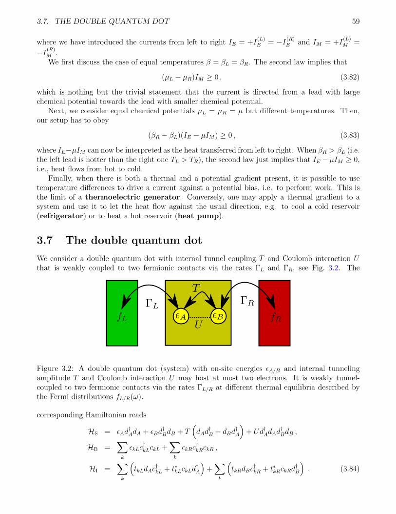
3.7. THE DOUBLE QUANTUM DOT 59
where we have introduced the currents from left to right IE = +I(L)E = −I(R)
E and IM = +I(L)M =
−I(R)M .We first discuss the case of equal temperatures β = βL = βR. The second law implies that
(µL − µR)IM ≥ 0 , (3.82)
which is nothing but the trivial statement that the current is directed from a lead with largechemical potential towards the lead with smaller chemical potential.
Next, we consider equal chemical potentials µL = µR = µ but different temperatures. Then,our setup has to obey
(βR − βL)(IE − µIM) ≥ 0 , (3.83)
where IE−µIM can now be interpreted as the heat transferred from left to right. When βR > βL (i.e.the left lead is hotter than the right one TL > TR), the second law just implies that IE −µIM ≥ 0,i.e., heat flows from hot to cold.
Finally, when there is both a thermal and a potential gradient present, it is possible to usetemperature differences to drive a current against a potential bias, i.e. to perform work. This isthe limit of a thermoelectric generator. Conversely, one may apply a thermal gradient to asystem and use it to let the heat flow against the usual direction, e.g. to cool a cold reservoir(refrigerator) or to heat a hot reservoir (heat pump).
3.7 The double quantum dot
We consider a double quantum dot with internal tunnel coupling T and Coulomb interaction Uthat is weakly coupled to two fermionic contacts via the rates ΓL and ΓR, see Fig. 3.2. The
Figure 3.2: A double quantum dot (system) with on-site energies εA/B and internal tunnelingamplitude T and Coulomb interaction U may host at most two electrons. It is weakly tunnel-coupled to two fermionic contacts via the rates ΓL/R at different thermal equilibria described bythe Fermi distributions fL/R(ω).
corresponding Hamiltonian reads
HS = εAd†AdA + εBd
†BdB + T
(dAd
†B + dBd
†A
)+ Ud†AdAd
†BdB ,
HB =∑k
εkLc†kLckL +
∑k
εkRc†kRckR ,
HI =∑k
(tkLdAc
†kL + t∗kLckLd
†A
)+∑k
(tkRdBc
†kR + t∗kRckRd
†B
). (3.84)
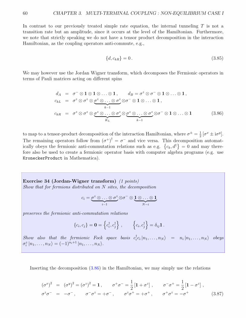
60 CHAPTER 3. MULTI-TERMINAL COUPLING : NON-EQUILIBRIUM CASE I
In contrast to our previously treated simple rate equation, the internal tunneling T is not atransition rate but an amplitude, since it occurs at the level of the Hamiltonian. Furthermore,we note that strictly speaking we do not have a tensor product decomposition in the interactionHamiltonian, as the coupling operators anti-commute, e.g.,
d, ckR = 0 . (3.85)
We may however use the Jordan Wigner transform, which decomposes the Fermionic operators interms of Pauli matrices acting on different spins
dA = σ− ⊗ 1⊗ 1⊗ . . .⊗ 1 , dB = σz ⊗ σ− ⊗ 1⊗ . . .⊗ 1 ,
ckL = σz ⊗ σz ⊗ σz ⊗ . . .⊗ σz︸ ︷︷ ︸k−1
⊗σ− ⊗ 1⊗ . . .⊗ 1 ,
ckR = σz ⊗ σz ⊗ σz ⊗ . . .⊗ σz︸ ︷︷ ︸KL
⊗σz ⊗ . . .⊗ σz︸ ︷︷ ︸k−1
⊗σ− ⊗ 1⊗ . . .⊗ 1 (3.86)
to map to a tensor-product decomposition of the interaction Hamiltonian, where σ± = 12
[σx ± iσy].
The remaining operators follow from (σ+)†
= σ− and vice versa. This decomposition automat-ically obeys the fermionic anti-commutation relations such as e.g.
ck, d
† = 0 and may there-fore also be used to create a fermionic operator basis with computer algebra programs (e.g. useKroneckerProduct in Mathematica).
Exercise 34 (Jordan-Wigner transform) (1 points)Show that for fermions distributed on N sites, the decomposition
ci = σz ⊗ . . .⊗ σz︸ ︷︷ ︸i−1
⊗σ− ⊗ 1⊗ . . .⊗ 1︸ ︷︷ ︸N−i
preserves the fermionic anti-commutation relations
ci, cj = 0 =c†i , c
†j
,
ci, c
†j
= δij1 .
Show also that the fermionic Fock space basis c†ici |n1, . . . , nN〉 = ni |n1, . . . , nN〉 obeysσzi |n1, . . . , nN〉 = (−1)ni+1 |n1, . . . , nN〉.
Inserting the decomposition (3.86) in the Hamiltonian, we may simply use the relations
(σx)2 = (σy)2 = (σz)2 = 1 , σ+σ− =1
2[1 + σz] , σ−σ+ =
1
2[1− σz] ,
σzσ− = −σ− , σ−σz = +σ− , σzσ+ = +σ+ , σ+σz = −σ+ (3.87)
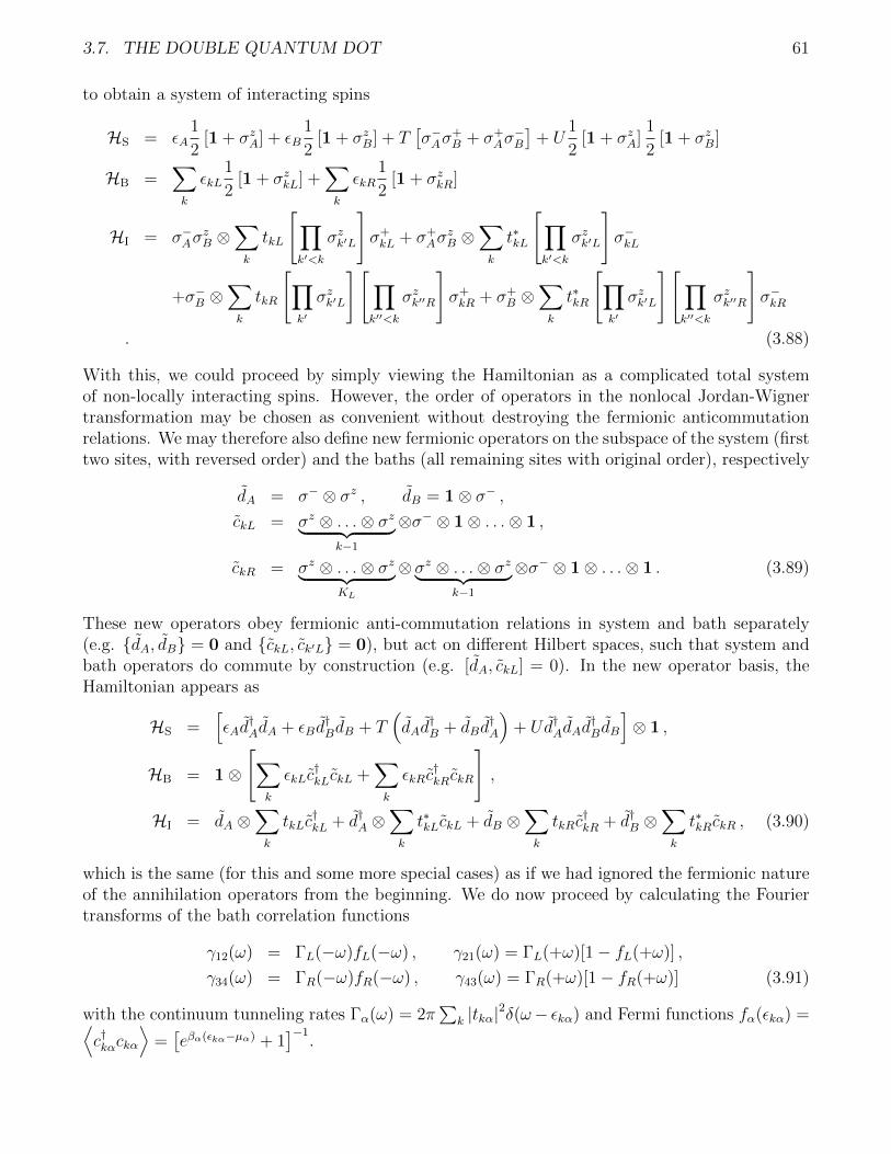
3.7. THE DOUBLE QUANTUM DOT 61
to obtain a system of interacting spins
HS = εA1
2[1 + σzA] + εB
1
2[1 + σzB] + T
[σ−Aσ
+B + σ+
Aσ−B
]+ U
1
2[1 + σzA]
1
2[1 + σzB]
HB =∑k
εkL1
2[1 + σzkL] +
∑k
εkR1
2[1 + σzkR]
HI = σ−AσzB ⊗
∑k
tkL
[∏k′<k
σzk′L
]σ+kL + σ+
AσzB ⊗
∑k
t∗kL
[∏k′<k
σzk′L
]σ−kL
+σ−B ⊗∑k
tkR
[∏k′
σzk′L
][∏k′′<k
σzk′′R
]σ+kR + σ+
B ⊗∑k
t∗kR
[∏k′
σzk′L
][∏k′′<k
σzk′′R
]σ−kR
. (3.88)
With this, we could proceed by simply viewing the Hamiltonian as a complicated total systemof non-locally interacting spins. However, the order of operators in the nonlocal Jordan-Wignertransformation may be chosen as convenient without destroying the fermionic anticommutationrelations. We may therefore also define new fermionic operators on the subspace of the system (firsttwo sites, with reversed order) and the baths (all remaining sites with original order), respectively
dA = σ− ⊗ σz , dB = 1⊗ σ− ,ckL = σz ⊗ . . .⊗ σz︸ ︷︷ ︸
k−1
⊗σ− ⊗ 1⊗ . . .⊗ 1 ,
ckR = σz ⊗ . . .⊗ σz︸ ︷︷ ︸KL
⊗σz ⊗ . . .⊗ σz︸ ︷︷ ︸k−1
⊗σ− ⊗ 1⊗ . . .⊗ 1 . (3.89)
These new operators obey fermionic anti-commutation relations in system and bath separately(e.g. dA, dB = 0 and ckL, ck′L = 0), but act on different Hilbert spaces, such that system andbath operators do commute by construction (e.g. [dA, ckL] = 0). In the new operator basis, theHamiltonian appears as
HS =[εAd
†AdA + εBd
†BdB + T
(dAd
†B + dBd
†A
)+ Ud†AdAd
†BdB
]⊗ 1 ,
HB = 1⊗
[∑k
εkLc†kLckL +
∑k
εkRc†kRckR
],
HI = dA ⊗∑k
tkLc†kL + d†A ⊗
∑k
t∗kLckL + dB ⊗∑k
tkRc†kR + d†B ⊗
∑k
t∗kRckR , (3.90)
which is the same (for this and some more special cases) as if we had ignored the fermionic natureof the annihilation operators from the beginning. We do now proceed by calculating the Fouriertransforms of the bath correlation functions
γ12(ω) = ΓL(−ω)fL(−ω) , γ21(ω) = ΓL(+ω)[1− fL(+ω)] ,
γ34(ω) = ΓR(−ω)fR(−ω) , γ43(ω) = ΓR(+ω)[1− fR(+ω)] (3.91)
with the continuum tunneling rates Γα(ω) = 2π∑
k |tkα|2δ(ω− εkα) and Fermi functions fα(εkα) =⟨
c†kαckα
⟩=[eβα(εkα−µα) + 1
]−1.
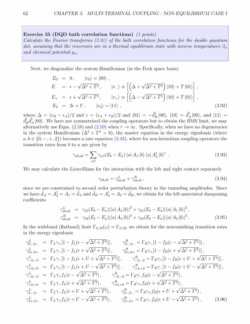
62 CHAPTER 3. MULTI-TERMINAL COUPLING : NON-EQUILIBRIUM CASE I
Exercise 35 (DQD bath correlation functions) (1 points)Calculate the Fourier transforms (3.91) of the bath correlation functions for the double quantumdot, assuming that the reservoirs are in a thermal equilibrium state with inverse temperatures βαand chemical potential µα.
Next, we diagonalize the system Hamiltonian (in the Fock space basis)
E0 = 0 , |v0〉 = |00〉 ,
E− = ε−√
∆2 + T 2 , |v−〉 ∝[(
∆ +√
∆2 + T 2)|10〉+ T |01〉
],
E+ = ε+√
∆2 + T 2 , |v+〉 ∝[(
∆−√
∆2 + T 2)|10〉+ T |01〉
],
E2 = 2ε+ U , |v2〉 = |11〉 , (3.92)
where ∆ = (εB − εA)/2 and ε = (εA + εB)/2 and |01〉 = −d†B |00〉, |10〉 = d†A |00〉, and |11〉 =d†Bd
†A |00〉. We have not symmetrized the coupling operators but to obtain the BMS limit, we may
alternatively use Eqns. (2.58) and (2.59) when τ →∞ . Specifically, when we have no degeneraciesin the system Hamiltonian (∆2 + T 2 > 0), the master equation in the energy eigenbasis (wherea, b ∈ 0,−,+, 2) becomes a rate equation (2.43), where for non-hermitian coupling operators thetransition rates from b to a are given by
γab,ab =∑αβ
γαβ(Eb − Ea) 〈a|Aβ |b〉 〈a|A†α |b〉∗ . (3.93)
We may calculate the Liouvillians for the interaction with the left and right contact separately
γab,ab = γLab,ab + γRab,ab , (3.94)
since we are constrained to second order perturbation theory in the tunneling amplitudes. Sincewe have dA = A†2 = A1 = dA and dB = A†4 = A2 = dB, we obtain for the left-associated dampeningcoefficients
γLab,ab = γ12(Eb − Ea)|〈a|A2 |b〉|2 + γ21(Eb − Ea)|〈a|A1 |b〉|2 ,γRab,ab = γ34(Eb − Ea)|〈a|A4 |b〉|2 + γ43(Eb − Ea)|〈a|A3 |b〉|2 . (3.95)
In the wideband (flatband) limit ΓL/R(ω) = ΓL/R, we obtain for the nonvanishing transition ratesin the energy eigenbasis
γL0−,0− = ΓLγ+[1− fL(ε−√
∆2 + T 2)] , γR0−,0− = ΓRγ−[1− fR(ε−√
∆2 + T 2)] ,
γL0+,0+ = ΓLγ−[1− fL(ε+√
∆2 + T 2)] , γR0+,0+ = ΓRγ+[1− fR(ε+√
∆2 + T 2)] ,
γL−2,−2 = ΓLγ−[1− fL(ε+ U +√
∆2 + T 2)] , γR−2,−2 = ΓRγ+[1− fR(ε+ U +√
∆2 + T 2)] ,
γL+2,+2 = ΓLγ+[1− fL(ε+ U −√
∆2 + T 2)] , γR+2,+2 = ΓRγ−[1− fR(ε+ U −√
∆2 + T 2)] ,
γL−0,−0 = ΓLγ+fL(ε−√
∆2 + T 2) , γR−0,−0 = ΓRγ−fR(ε−√
∆2 + T 2) ,
γL+0,+0 = ΓLγ−fL(ε+√
∆2 + T 2) , γR+0,+0 = ΓRγ+fR(ε+√
∆2 + T 2) ,
γL2−,2− = ΓLγ−fL(ε+ U +√
∆2 + T 2) , γR2−,2− = ΓRγ+fR(ε+ U +√
∆2 + T 2) ,
γL2+,2+ = ΓLγ+fL(ε+ U −√
∆2 + T 2) , γR2+,2+ = ΓRγ−fR(ε+ U −√
∆2 + T 2) , (3.96)
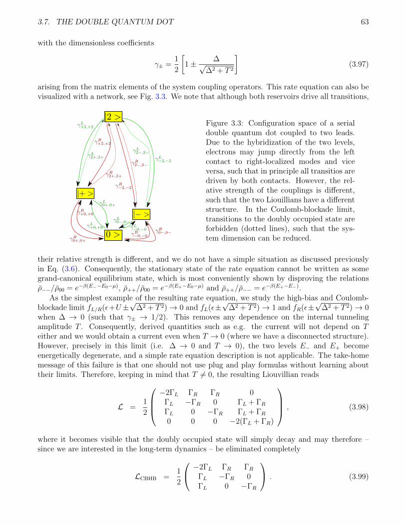
3.7. THE DOUBLE QUANTUM DOT 63
with the dimensionless coefficients
γ± =1
2
[1± ∆√
∆2 + T 2
](3.97)
arising from the matrix elements of the system coupling operators. This rate equation can also bevisualized with a network, see Fig. 3.3. We note that although both reservoirs drive all transitions,
Figure 3.3: Configuration space of a serialdouble quantum dot coupled to two leads.Due to the hybridization of the two levels,electrons may jump directly from the leftcontact to right-localized modes and viceversa, such that in principle all transitios aredriven by both contacts. However, the rel-ative strength of the couplings is different,such that the two Liouillians have a differentstructure. In the Coulomb-blockade limit,transitions to the doubly occupied state areforbidden (dotted lines), such that the sys-tem dimension can be reduced.
their relative strength is different, and we do not have a simple situation as discussed previouslyin Eq. (3.6). Consequently, the stationary state of the rate equation cannot be written as somegrand-canonical equilibrium state, which is most conveniently shown by disproving the relationsρ−−/ρ00 = e−β(E−−E0−µ), ρ++/ρ00 = e−β(E+−E0−µ) and ρ++/ρ−− = e−β(E+−E−).
As the simplest example of the resulting rate equation, we study the high-bias and Coulomb-blockade limit fL/R(ε+U±
√∆2 + T 2)→ 0 and fL(ε±
√∆2 + T 2)→ 1 and fR(ε±
√∆2 + T 2)→ 0
when ∆ → 0 (such that γ± → 1/2). This removes any dependence on the internal tunnelingamplitude T . Consequently, derived quantities such as e.g. the current will not depend on Teither and we would obtain a current even when T → 0 (where we have a disconnected structure).However, precisely in this limit (i.e. ∆ → 0 and T → 0), the two levels E− and E+ becomeenergetically degenerate, and a simple rate equation description is not applicable. The take-homemessage of this failure is that one should not use plug and play formulas without learning abouttheir limits. Therefore, keeping in mind that T 6= 0, the resulting Liouvillian reads
L =1
2
−2ΓL ΓR ΓR 0
ΓL −ΓR 0 ΓL + ΓRΓL 0 −ΓR ΓL + ΓR0 0 0 −2(ΓL + ΓR)
, (3.98)
where it becomes visible that the doubly occupied state will simply decay and may therefore –since we are interested in the long-term dynamics – be eliminated completely
LCBHB =1
2
−2ΓL ΓR ΓRΓL −ΓR 0ΓL 0 −ΓR
. (3.99)
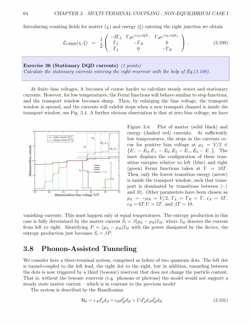
64 CHAPTER 3. MULTI-TERMINAL COUPLING : NON-EQUILIBRIUM CASE I
Introducing counting fields for matter (χ) and energy (ξ) entering the right junction we obtain
LCBHB(χ, ξ) =1
2
−2ΓL ΓRe+iχ+iξE− ΓRe
+iχ+iξE+
ΓL −ΓR 0ΓL 0 −ΓR
. (3.100)
Exercise 36 (Stationary DQD currents) (1 points)Calculate the stationary currents entering the right reservoir with the help of Eq.(3.100).
At finite bias voltages, it becomes of course harder to calculate steady states and stationarycurrents. However, for low temperatures, the Fermi functions will behave similiar to step functions,and the transport window becomes sharp. Then, by enlarging the bias voltage, the transportwindow is opened, and the currents will exhibit steps when a new transport channel is inside thetransport window, see Fig. 3.4. A further obvious observation is that at zero bias voltage, we have
-30 -20 -10 0 10 20 30
dimensionless bias voltage V/T
-2
-1
0
1
2
dim
ensi
onle
ss c
urr
ent
matter current I [Γ]
energy current [T Γ]
2 E-
2 E+
2(E2-E
+)
2(E2-E
-)
µR
µL
Figure 3.4: Plot of matter (solid black) andenergy (dashed red) currents. At sufficientlylow temperatures, the steps in the currents oc-cur for positive bias voltage at µL = V/2 ∈E− − E0, E+ − E0, E2 − E+, E2 − E−. Theinset displays the configuration of these tran-sition energies relative to left (blue) and right(green) Fermi functions taken at V = 10T .Then, only the lowest transition energy (arrow)is inside the transport window, such that trans-port is dominated by transitions between |−〉and |0〉. Other parameters have been chosen asµL = −µR = V/2, ΓL = ΓR = Γ, εA = 4T ,εB = 6T ,U = 5T , and βT = 10.
vanishing currents. This must happen only at equal temperatures. The entropy production in thiscase is fully determined by the matter current Si = β(µL − µR)IM , where IM denotes the currentfrom left to right. Identifying P = (µL − µR)IM with the power dissipated by the device, theentropy production just becomes Si = βP .
3.8 Phonon-Assisted Tunneling
We consider here a three-terminal system, comprised as before of two quantum dots. The left dotis tunnel-coupled to the left lead, the right dot to the right, but in addition, tunneling betweenthe dots is now triggered by a third (bosonic) reservoir that does not change the particle content.That is, without the bosonic reservoir (e.g. phonons or photons) the model would not support asteady state matter current – which is in contrast to the previous model
The system is described by the Hamiltonian
HS = εAd†AdA + εBd
†BdB + Ud†AdAd
†BdB (3.101)
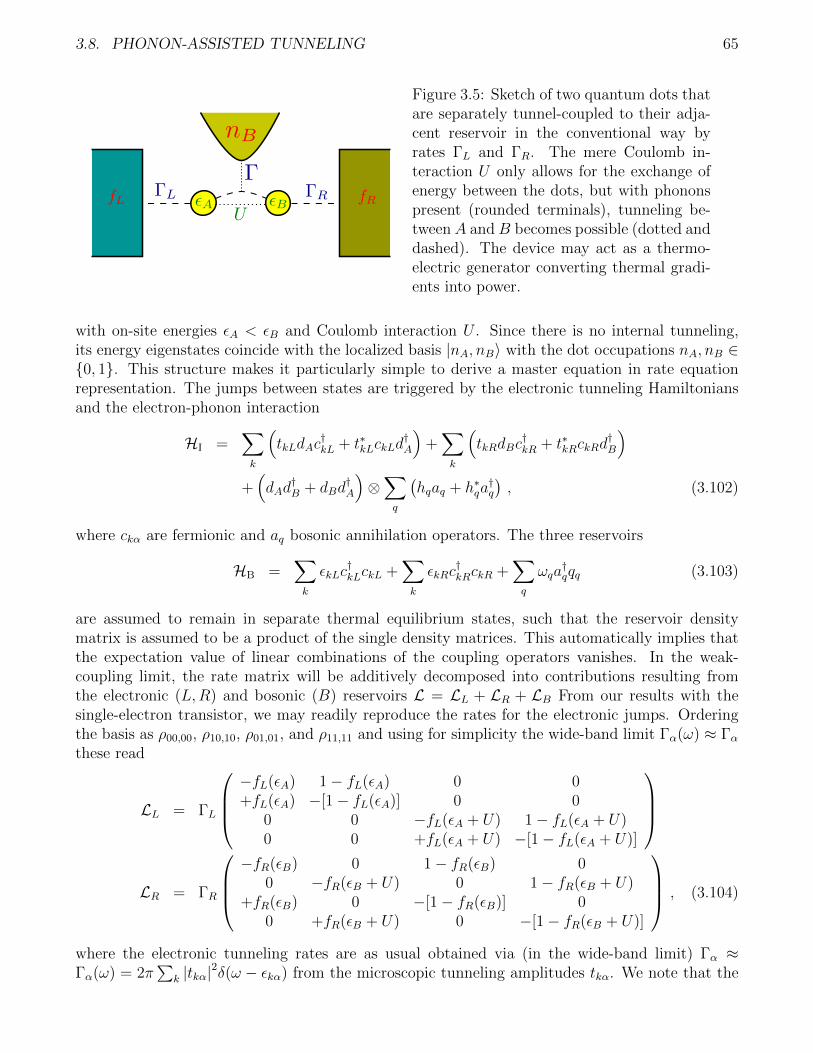
3.8. PHONON-ASSISTED TUNNELING 65
Figure 3.5: Sketch of two quantum dots thatare separately tunnel-coupled to their adja-cent reservoir in the conventional way byrates ΓL and ΓR. The mere Coulomb in-teraction U only allows for the exchange ofenergy between the dots, but with phononspresent (rounded terminals), tunneling be-tween A andB becomes possible (dotted anddashed). The device may act as a thermo-electric generator converting thermal gradi-ents into power.
with on-site energies εA < εB and Coulomb interaction U . Since there is no internal tunneling,its energy eigenstates coincide with the localized basis |nA, nB〉 with the dot occupations nA, nB ∈0, 1. This structure makes it particularly simple to derive a master equation in rate equationrepresentation. The jumps between states are triggered by the electronic tunneling Hamiltoniansand the electron-phonon interaction
HI =∑k
(tkLdAc
†kL + t∗kLckLd
†A
)+∑k
(tkRdBc
†kR + t∗kRckRd
†B
)+(dAd
†B + dBd
†A
)⊗∑q
(hqaq + h∗qa
†q
), (3.102)
where ckα are fermionic and aq bosonic annihilation operators. The three reservoirs
HB =∑k
εkLc†kLckL +
∑k
εkRc†kRckR +
∑q
ωqa†qqq (3.103)
are assumed to remain in separate thermal equilibrium states, such that the reservoir densitymatrix is assumed to be a product of the single density matrices. This automatically implies thatthe expectation value of linear combinations of the coupling operators vanishes. In the weak-coupling limit, the rate matrix will be additively decomposed into contributions resulting fromthe electronic (L,R) and bosonic (B) reservoirs L = LL + LR + LB From our results with thesingle-electron transistor, we may readily reproduce the rates for the electronic jumps. Orderingthe basis as ρ00,00, ρ10,10, ρ01,01, and ρ11,11 and using for simplicity the wide-band limit Γα(ω) ≈ Γαthese read
LL = ΓL
−fL(εA) 1− fL(εA) 0 0+fL(εA) −[1− fL(εA)] 0 0
0 0 −fL(εA + U) 1− fL(εA + U)0 0 +fL(εA + U) −[1− fL(εA + U)]
LR = ΓR
−fR(εB) 0 1− fR(εB) 0
0 −fR(εB + U) 0 1− fR(εB + U)+fR(εB) 0 −[1− fR(εB)] 0
0 +fR(εB + U) 0 −[1− fR(εB + U)]
, (3.104)
where the electronic tunneling rates are as usual obtained via (in the wide-band limit) Γα ≈Γα(ω) = 2π
∑k |tkα|
2δ(ω − εkα) from the microscopic tunneling amplitudes tkα. We note that the
66 CHAPTER 3. MULTI-TERMINAL COUPLING : NON-EQUILIBRIUM CASE I
Fermi functions are evaluated at the energy difference of the jump to which they refer. Althoughenergy may be transferred between the left and right junctions without the presence of phonons,it is not possible to transfer charges.
For the spin-boson example, we have also already calculated the correlation function for thephonons for a spin-boson model in Sec. 2.2.4. Since the reservoir coupling operator is identical, wemay use our result from Eq. (2.73).
γ(ω) = Γ(+ω)Θ(+ω)[1 + nB(+ω)] + Γ(−ω)Θ(−ω)nB(−ω) , (3.105)
where Γ(ω) = 2π∑
k |hk|2δ(ω−ωk) was the bosonic emission or absorption rate and nB(ω) denoted
the Bose-Einstein distribution function. For consistency, we just note that the KMS condition isobeyed. With this, we may readily evaluate the rates due to the phonon reservoirs, i.e., we havewith Γ = Γ(εB − εA)
LB = Γ
0 0 0 00 −nB(εB − εA) 1 + nB(εB − εA) 00 +nB(εB − εA) −[1 + nB(εB − εA)] 00 0 0 0
. (3.106)
The rate matrices in Eqs. (3.104) and (3.106) can be used to extract the full electron-phononcounting statistics after all jumps have been identified. We have a three terminal system, wherethe phonon terminal only allows for the exchange of energy, i.e., in total we can calculate fivenon-vanishing currents. With the conservation laws on matter and energy currents, we can atsteady state eliminate two of these, and the entropy production becomes
Si = −βphIBE − βL(ILE − µLILM)− βR(IRE − µRIRM)
= −βphIBE − βL(ILE − µLILM) + βR(ILE + IBE − µRILM)
= (βR − βph)IBE + (βR − βL)ILE + (βLµL − βRµR)ILM , (3.107)
which has the characteristic affinity-flux form. In usual electronic setups, the electronic tempera-tures will be the same βel = βL = βR, such that the entropy production further reduces to
Si = (βel − βph)IBE + βel(µL − µR)ILM ≥ 0 , (3.108)
where we can identify the term (µL − µR)ILM as a power consumed or produced by the device.Furthermore, we note that the device obeys the tight-coupling property: Every electron traversingthe system from left to right must absorb energy εB−εA from the phonon reservoir IBE = (εB−εA)ILM .Therefore, the entropy production can also be written as
Si = [(βel − βph)(εB − εA) + βel(µL − µR)] ILM ≥ 0 . (3.109)
We note that the prefactor of the matter current vanishes at
V ∗ = µ∗L − µ∗R =
(Tel
Tph
− 1
)(εB − εA) . (3.110)
Since the prefactor switches sign at this voltage, the matter current must vanish at this voltage, too– otherwise the entropy production would not be positive. Without calculation, we have thereforefound that at bias voltage V ∗ the current must vanish.
3.8. PHONON-ASSISTED TUNNELING 67
For simplicity, we decide to count matter at the left junction (χ) and energy transfers at thebosonic junction (ξ). To keep a compact description, we introduce the abbreviations
nB = nB(εB − εA) , fL = fL(εA) , fR = fR(εB) ,
fL = fL(εA + U) , fR = fR(εB + U) , Γ = Γ(εB − εA) . (3.111)
With the counting fields, the complete system then becomes
L = ΓL
−fL (1− fL)e−iχ 0 0
+fLe+iχ −[1− fL] 0 0
0 0 −fL (1− fL)e−iχ
0 0 +fLe+iχ −(1− fL)
+Γ
0 0 0 00 −nB (1 + nB)e−i(εB−εA)ξ 00 +nBe
+i(εB−εA)ξ −(1 + nB) 00 0 0 0
+ΓR
−fR 0 1− fR 0
0 −fR 0 1− fR+fR 0 −(1− fR) 0
0 +fR 0 −(1− fR)
. (3.112)
Noting that the total entropy production is positive does not imply that all contributions areseparately positive. Fig. 3.6 displays the current as a function of the bias voltage for differentelectronic and phonon temperature configurations. It is visible that at zero bias, the mattercurrent does not vanish when electron and phonon temperatures are not chosen equal.
3.8.1 Thermoelectric performance
We concentrate on the simple case discussed before and use βL = βR = βel and βph = βB. Inregions where the current runs against the bias, the power
P = −(µL − µR)ILM (3.113)
becomes positive, and we can define an efficiency via
η =−(µL − µR)ILM
Qin
Θ(P ) , (3.114)
where Qin is the heat entering the system from the hot reservoir. The purpose of the Heavisidefunction is just to avoid misinterpretations of the efficiency.
Consequently, when the phonon temperature is larger than the electron temperature Tph > Tel,the input heat is given by the positive energy flow from the hot phonon bath into the system, suchthat – due to the tight-coupling property – the efficiency becomes trivially dependent on the biasvoltage
ηTph>Tel=
P
IBEΘ(P ) = − V
εB − εAΘ(P ) . (3.115)
At first sight, one might think that this efficiency could become larger than one. It should be keptin mind however that it is only valid in regimes where the power (3.113) is positive, which limits
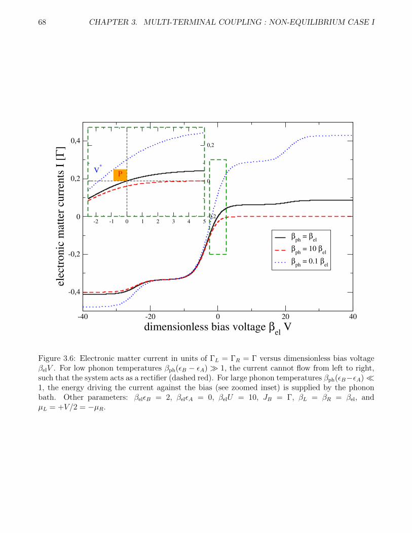
68 CHAPTER 3. MULTI-TERMINAL COUPLING : NON-EQUILIBRIUM CASE I
-40 -20 0 20 40
dimensionless bias voltage βel
V
-0,4
-0,2
0
0,2
0,4
elec
tro
nic
mat
ter
curr
ents
I [
Γ]
βph
= βel
βph
= 10 βel
βph
= 0.1 βel
-2 -1 0 1 2 3 4 5-0,2
0
0,2
V*
P
Figure 3.6: Electronic matter current in units of ΓL = ΓR = Γ versus dimensionless bias voltageβelV . For low phonon temperatures βph(εB − εA) 1, the current cannot flow from left to right,such that the system acts as a rectifier (dashed red). For large phonon temperatures βph(εB−εA)1, the energy driving the current against the bias (see zoomed inset) is supplied by the phononbath. Other parameters: βelεB = 2, βelεA = 0, βelU = 10, JB = Γ, βL = βR = βel, andµL = +V/2 = −µR.
3.9. FLUCTUATION THEOREMS 69
the applicability of these efficiencies to voltages within V = 0 and V = V ∗ from Eq. (3.110). Themaximum efficiency is reached at V = V ∗ and reads
ηTph>Tel< 1− Tel
Tph
= ηCa , (3.116)
and is thus upper-bounded by Carnot efficiency
ηCa = 1− Tcold
Thot
. (3.117)
In the opposite case, where Tph < Tel, the input heat is given by the sum of the energy currentsentering from the hot electronic leads Qin = QL + QR = ILE + IRE + P = −IBE + P , such that theefficiency becomes
ηTph<Tel=
P
−IBE + P=
(µL − µR)
(εB − εA) + (µL − µR)=
1
1 + εB−εAµL−µR
, (3.118)
which also trivially depends on the bias voltage. Inserting the maximum bias voltage with positivepower in Eq. (3.110) we obtain the maximum efficiency
ηTph<Tel<
1
1 + 1TelTph−1
= 1− Tph
Tel
, (3.119)
which is also just the Carnot efficiency.
Unfortunately, Carnot efficiencies are reached at vanishing current, i.e., at zero power. Atthese parameters, a thermoelectric device is useless. It is therefore more practical to consider theefficiency at maximum power. However, since the currents depend in a highly nonlinear fashion onall parameters (coupling constants, temperatures, chemical potentials, and system parameters),this becomes a numerical optimization problem – unless one restricts the analysis to the linearresponse regime.
3.9 Fluctuation Theorems
The probability distribution Pn(t) is given by the inverse Fourier transform of the moment-generating function
Pn(t) =1
2π
+π∫−π
M(χ, t)e−inχdχ =1
2π
+π∫−π
eC(χ,t)−inχdχ . (3.120)
Accordingly, a symmetry in the cumulant-generating function (or moment-generating function) ofthe form
C(−χ, t) = C(+χ+ iα, t) (3.121)
70 CHAPTER 3. MULTI-TERMINAL COUPLING : NON-EQUILIBRIUM CASE I
leads to a symmetry of the probabilities
P+n(t)
P−n(t)=
12π
∫ +π
−π eC(χ,t)−inχdχ
12π
∫ +π
−π eC(χ,t)+inχdχ
=
∫ +π
−π eC(χ,t)−inχdχ∫ +π
−π eC(−χ,t)−inχdχ
=
∫ +π
−π eC(χ,t)−inχdχ∫ +π
−π eC(χ+iα,t)−inχdχ
=
∫ +π
−π eC(χ,t)−inχdχ∫ +π+iα
−π+iαeC(χ,t)−in[χ−iα]dχ
=
∫ +π
−π eC(χ,t)−inχdχ
e−nα∫ +π
−π eC(χ,t)−inχdχ
= e+nα , (3.122)
where we have used in the last step that the counting field always enters as a function of e±iχ.This automatically implies that C(−π + iσ, t) = C(+π + iσ, t) for all real numbers σ, such thatwe can add two further integration paths from −π to −π + iα and from +π + iα to +π to theintegral in the denominator. The value of the cumulant-generating function along these pathsis the same, such that due to the different integral orientation there is no net change. Finally,using analyticity of the integrand, we deform the integration contour in the denominator, leavingtwo identical integrals in numerator and denominator. Note that the system may be very farfrom thermodynamic equilibrium but still obey a symmetry of the form (3.121), which leads to afluctuation theorem of the form (3.122) being valid far from equilibrium.
As example, we consider the SET (which is always in thermal equilibrium). The characteristicpolynomial D(χ) = |L(χ)− λ1| of the Liouvillian (3.20) and therefore also all eigenvalues obeysthe symmetry
D(−χ) = D(
+χ+ i ln
[fL(1− fR)
(1− fL)fR
])= D (χ+ i [(βR − βL) ε+ βLµL − βRµR]) . (3.123)
Exercise 37 (Eigenvalue Symmetry) (1 points)Compute the characteristic polynomial of the Liouvillian (3.20) and confirm the symmetry (3.123).
which leads to the fluctuation theorem
limt→∞
P+n(t)
P−n(t)= en[(βR−βL)ε+βLµL−βRµR] . (3.124)
We note that the exponent does not depend on the microscopic details of the model (ε, Γα) butonly on the thermodynamic quantities. We would obtain the same result for a DQD coupled totwo terminals. For equal temperatures, this becomes
limt→∞
P+n(t)
P−n(t)= enβV , (3.125)
which directly demonstrates that the average current
I =d
dt〈n(t)〉 =
d
dt
+∞∑n=−∞
nPn(t) =∞∑n=1
n [P+n(t)− P−n(t)] =∞∑n=1
nPn(t)[1− e−nβV
](3.126)
3.9. FLUCTUATION THEOREMS 71
always follows the voltage. We can interpret the exponent in Eq. (3.124) in terms of the entropythat has been produced: The quantity nε describes the energy that has traversed the SET for largetimes, and consequently, the term in the exponent approximates the entropy production, which isfor large times simply proportional to the number of particles that have travelled from left to right
∆Si ≈ (βR − βL)nε+ (βLµL − βRµR)n . (3.127)
Therefore, we can interpret the fluctuation theorem also as a stochastic manifestation of the secondlaw
P (+∆Si)
P (−∆Si)= e+∆Si . (3.128)
Here, trajectories with a negative entropy production ∆Si are not forbidden. They are just lesslikely to occur than their positive-production counterparts, such that – on average – the secondlaw is always obeyed.
The SET has the property of tight coupling between enery and matter currents: Everyelectron carries the same energy. For more general systems, where this property is not present,one still obtains a fluctuation theorem for the entropy production. Then, the combined countingstatistics of energy and matter currents is necessary to obtain it. Furthermore, one will for ann-terminal system need 2n counting fields to quantify the entropy production. In the long-termlimit, one can use conservation laws, such that the maximum number of counting fields is givenby 2n− 2, which can be further reduced when one has further symmetries (like tight-coupling).
Exercise 38 (Fluctuation Theorem) (1 points)Calculate the long-term fluctuation theorem for Eq. (3.112) in the Coulomb-blockade regime fα →0, when only matter transfer from left to right is counted. To do so, first reduce the dimension ofthe system (Coulomb blockade). Then, introduce a matter counting field at the junction of yourchoice and try to find a symmetry of the characteristic polynomial.

72 CHAPTER 3. MULTI-TERMINAL COUPLING : NON-EQUILIBRIUM CASE I
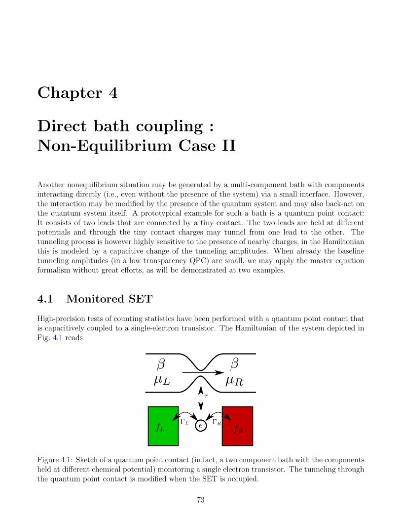
Chapter 4
Direct bath coupling :Non-Equilibrium Case II
Another nonequilibrium situation may be generated by a multi-component bath with componentsinteracting directly (i.e., even without the presence of the system) via a small interface. However,the interaction may be modified by the presence of the quantum system and may also back-act onthe quantum system itself. A prototypical example for such a bath is a quantum point contact:It consists of two leads that are connected by a tiny contact. The two leads are held at differentpotentials and through the tiny contact charges may tunnel from one lead to the other. Thetunneling process is however highly sensitive to the presence of nearby charges, in the Hamiltonianthis is modeled by a capacitive change of the tunneling amplitudes. When already the baselinetunneling amplitudes (in a low transparency QPC) are small, we may apply the master equationformalism without great efforts, as will be demonstrated at two examples.
4.1 Monitored SET
High-precision tests of counting statistics have been performed with a quantum point contact thatis capacitively coupled to a single-electron transistor. The Hamiltonian of the system depicted inFig. 4.1 reads
Figure 4.1: Sketch of a quantum point contact (in fact, a two component bath with the componentsheld at different chemical potential) monitoring a single electron transistor. The tunneling throughthe quantum point contact is modified when the SET is occupied.
73
74 CHAPTER 4. DIRECT BATH COUPLING : NON-EQUILIBRIUM CASE II
HS = εd†d ,
HB =∑k
εkLc†kLckL +
∑k
εkLc†kRckR +
∑k
εkLγ†kLγkL +
∑k
εkLγ†kRγkR ,
HI =
[∑k
tkLdc†kL +
∑k
tkRdc†kR + h.c.
]+
[∑kk′
(tkk′ + d†dτkk′
)γkLγ
†k′R + h.c.
], (4.1)
where ε denotes the dot level, ckα annihilate electrons on SET lead α and γkα are the annihilationoperators for the QPC lead α. The QPC baseline tunneling amplitude is given by tkk′ and describesthe scattering of and electron from mode k in the left lead to mode k′ in the right QPC contact.When the nearby SET is occupied it is modified to tkk′ + τkk′ , where τkk′ represents the change ofthe tunneling amplitude.
We will derive a master equation for the dynamics of the SET due to the interaction with theQPC and the two SET contacts. In addition, we are interested not only in the charge countingstatistics of the SET but also the QPC. The Liouvillian for the SET-contact interaction is wellknown and has been stated previously (we insert counting fields at the right lead to count chargestraversing the SET from left to right)
LSET(χ) =
(−ΓLfL − ΓRfR +ΓL(1− fL) + ΓR(1− fR)e+iχ
+ΓLfL + ΓRfRe−iχ −ΓL(1− fL)− ΓR(1− fR)
). (4.2)
We will therefore derive the dissipator for the SET-QPC interaction separately. To keep trackof the tunneled QPC electrons, we insert a virtual detector operator in the respective tunnelingHamiltonian
HQPCI =
∑kk′
(tkk′1 + d†dτkk′
)B†γkLγ
†k′R +
∑kk′
(t∗kk′1 + d†dτ ∗kk′
)Bγk′Rγ
†kL
= 1⊗B† ⊗∑kk′
tkk′γkLγ†k′R + 1⊗B ⊗
∑kk′
t∗kk′γk′Rγ†kL
+d†d⊗B† ⊗∑kk′
τkk′γkLγ†k′R + d†d⊗B ⊗
∑kk′
τ ∗kk′γk′Rγ†kL . (4.3)
Note that we have implicitly performed the mapping to a tensor product representation of thefermionic operators, which is unproblematic here as between SET and QPC no particle exchangetakes place and the electrons in the QPC and the SET may be treated as different particle types.To simplify the system, we assume that the change of tunneling amplitudes affects all modes inthe same manner, i.e., τkk′ = τ tkk′ , which enables us to combine some coupling operators
HQPCI =
[1 + τ d†d
]⊗B† ⊗
∑kk′
tkk′γkLγ†k′R +
[1 + τ ∗d†d
]⊗B ⊗
∑kk′
t∗kk′γk′Rγ†kL . (4.4)
The evident advantage of this approximation is that only two correlation functions have to becomputed. We can now straightforwardly (since the baseline tunneling term is not included in thebath Hamiltonian) map to the interaction picture
B1(τ) =∑kk′
tkk′γkLγ†k′Re
−i(εkL−εk′R)τ , B2(τ) =∑kk′
t∗kk′γk′Rγ†kLe
+i(εkL−εk′R)τ . (4.5)
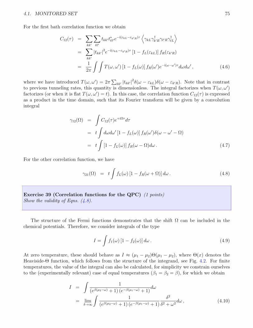
4.1. MONITORED SET 75
For the first bath correlation function we obtain
C12(τ) =∑kk′
∑``′
tkk′t∗``′e−i(εkL−εk′R)τ
⟨γkLγ
†k′Rγ`′Rγ
†`L
⟩=
∑kk′
|tkk′|2e−i(εkL−εk′R)τ [1− fL(εkL)] fR(εk′R)
=1
2π
∫ ∫T (ω, ω′) [1− fL(ω)] fR(ω′)e−i(ω−ω′)τdωdω′ , (4.6)
where we have introduced T (ω, ω′) = 2π∑
kk′ |tkk′ |2δ(ω − εkL)δ(ω − εk′R). Note that in contrast
to previous tunneling rates, this quantity is dimensionless. The integral factorizes when T (ω, ω′)factorizes (or when it is flat T (ω, ω′) = t). In this case, the correlation function C12(τ) is expressedas a product in the time domain, such that its Fourier transform will be given by a convolutionintegral
γ12(Ω) =
∫C12(τ)e+iΩτdτ
= t
∫dωdω′ [1− fL(ω)] fR(ω′)δ(ω − ω′ − Ω)
= t
∫[1− fL(ω)] fR(ω − Ω)dω . (4.7)
For the other correlation function, we have
γ21(Ω) = t
∫fL(ω) [1− fR(ω + Ω)] dω . (4.8)
Exercise 39 (Correlation functions for the QPC) (1 points)Show the validity of Eqns. (4.8).
The structure of the Fermi functions demonstrates that the shift Ω can be included in thechemical potentials. Therefore, we consider integrals of the type
I =
∫f1(ω) [1− f2(ω)] dω . (4.9)
At zero temperature, these should behave as I ≈ (µ1 − µ2)Θ(µ1 − µ2), where Θ(x) denotes theHeaviside-Θ function, which follows from the structure of the integrand, see Fig. 4.2. For finitetemperatures, the value of the integral can also be calculated, for simplicity we constrain ourselvesto the (experimentally relevant) case of equal temperatures (β1 = β2 = β), for which we obtain
I =
∫1
(eβ(µ2−ω) + 1) (e−β(µ1−ω) + 1)dω
= limδ→∞
∫1
(eβ(µ2−ω) + 1) (e−β(µ1−ω) + 1)
δ2
δ2 + ω2dω , (4.10)
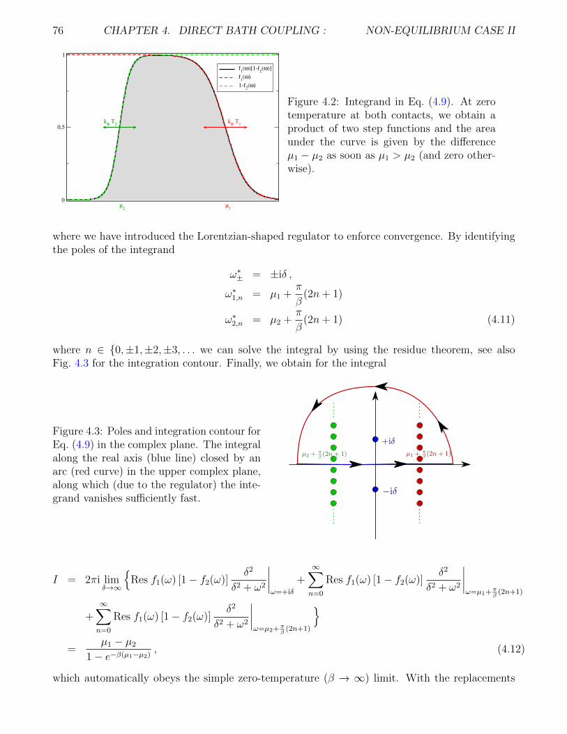
76 CHAPTER 4. DIRECT BATH COUPLING : NON-EQUILIBRIUM CASE II
0
0,5
1
µ2
µ1
f1(ω)[1-f
2(ω)]
f1(ω)
1-f2(ω)
kB T
2k
B T
1
Figure 4.2: Integrand in Eq. (4.9). At zerotemperature at both contacts, we obtain aproduct of two step functions and the areaunder the curve is given by the differenceµ1 − µ2 as soon as µ1 > µ2 (and zero other-wise).
where we have introduced the Lorentzian-shaped regulator to enforce convergence. By identifyingthe poles of the integrand
ω∗± = ±iδ ,
ω∗1,n = µ1 +π
β(2n+ 1)
ω∗2,n = µ2 +π
β(2n+ 1) (4.11)
where n ∈ 0,±1,±2,±3, . . . we can solve the integral by using the residue theorem, see alsoFig. 4.3 for the integration contour. Finally, we obtain for the integral
Figure 4.3: Poles and integration contour forEq. (4.9) in the complex plane. The integralalong the real axis (blue line) closed by anarc (red curve) in the upper complex plane,along which (due to the regulator) the inte-grand vanishes sufficiently fast.
I = 2πi limδ→∞
Res f1(ω) [1− f2(ω)]
δ2
δ2 + ω2
∣∣∣∣ω=+iδ
+∞∑n=0
Res f1(ω) [1− f2(ω)]δ2
δ2 + ω2
∣∣∣∣ω=µ1+π
β(2n+1)
+∞∑n=0
Res f1(ω) [1− f2(ω)]δ2
δ2 + ω2
∣∣∣∣ω=µ2+π
β(2n+1)
=
µ1 − µ2
1− e−β(µ1−µ2), (4.12)
which automatically obeys the simple zero-temperature (β → ∞) limit. With the replacements
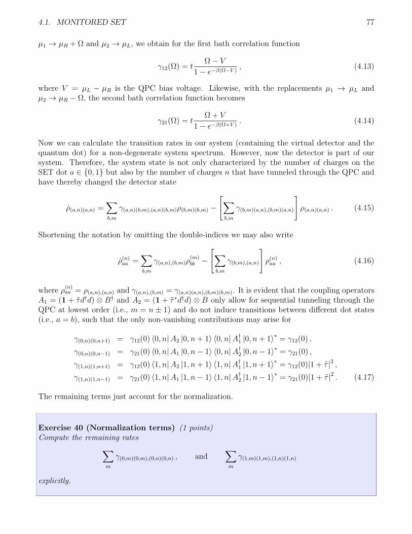
4.1. MONITORED SET 77
µ1 → µR + Ω and µ2 → µL, we obtain for the first bath correlation function
γ12(Ω) = tΩ− V
1− e−β(Ω−V ), (4.13)
where V = µL − µR is the QPC bias voltage. Likewise, with the replacements µ1 → µL andµ2 → µR − Ω, the second bath correlation function becomes
γ21(Ω) = tΩ + V
1− e−β(Ω+V ). (4.14)
Now we can calculate the transition rates in our system (containing the virtual detector and thequantum dot) for a non-degenerate system spectrum. However, now the detector is part of oursystem. Therefore, the system state is not only characterized by the number of charges on theSET dot a ∈ 0, 1 but also by the number of charges n that have tunneled through the QPC andhave thereby changed the detector state
ρ(a,n)(a,n) =∑b,m
γ(a,n)(b,m),(a,n)(b,m)ρ(b,m)(b,m) −
[∑b,m
γ(b,m)(a,n),(b,m)(a,n)
]ρ(a,n)(a,n) . (4.15)
Shortening the notation by omitting the double-indices we may also write
ρ(n)aa =
∑b,m
γ(a,n),(b,m)ρ(m)bb −
[∑b,m
γ(b,m),(a,n)
]ρ(n)aa , (4.16)
where ρ(n)aa = ρ(a,n),(a,n) and γ(a,n),(b,m) = γ(a,n)(a,n),(b,m)(b,m). It is evident that the coupling operators
A1 = (1 + τ d†d) ⊗ B† and A2 = (1 + τ ∗d†d) ⊗ B only allow for sequential tunneling through theQPC at lowest order (i.e., m = n ± 1) and do not induce transitions between different dot states(i.e., a = b), such that the only non-vanishing contributions may arise for
γ(0,n)(0,n+1) = γ12(0) 〈0, n|A2 |0, n+ 1〉 〈0, n|A†1 |0, n+ 1〉∗ = γ12(0) ,
γ(0,n)(0,n−1) = γ21(0) 〈0, n|A1 |0, n− 1〉 〈0, n|A†2 |0, n− 1〉∗ = γ21(0) ,
γ(1,n)(1,n+1) = γ12(0) 〈1, n|A2 |1, n+ 1〉 〈1, n|A†1 |1, n+ 1〉∗ = γ12(0)|1 + τ |2 ,γ(1,n)(1,n−1) = γ21(0) 〈1, n|A1 |1, n− 1〉 〈1, n|A†2 |1, n− 1〉∗ = γ21(0)|1 + τ |2 . (4.17)
The remaining terms just account for the normalization.
Exercise 40 (Normalization terms) (1 points)Compute the remaining rates∑
m
γ(0,m)(0,m),(0,n)(0,n) , and∑m
γ(1,m)(1,m),(1,n)(1,n)
explicitly.
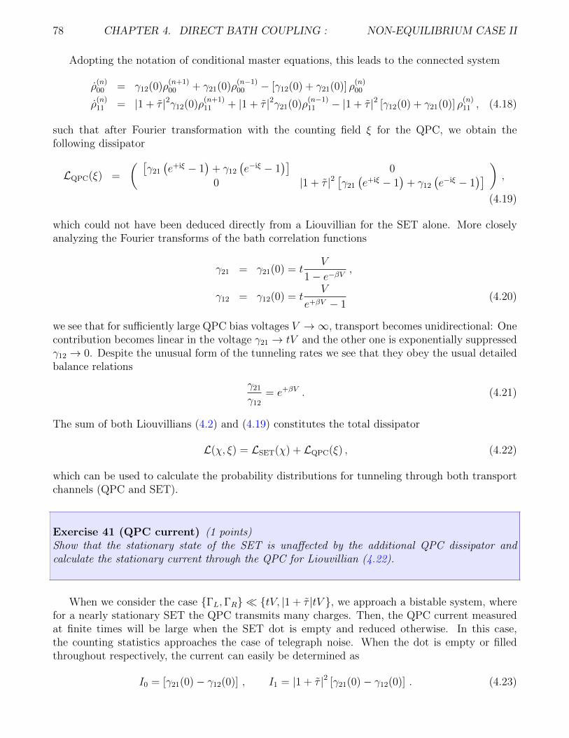
78 CHAPTER 4. DIRECT BATH COUPLING : NON-EQUILIBRIUM CASE II
Adopting the notation of conditional master equations, this leads to the connected system
ρ(n)00 = γ12(0)ρ
(n+1)00 + γ21(0)ρ
(n−1)00 − [γ12(0) + γ21(0)] ρ
(n)00
ρ(n)11 = |1 + τ |2γ12(0)ρ
(n+1)11 + |1 + τ |2γ21(0)ρ
(n−1)11 − |1 + τ |2 [γ12(0) + γ21(0)] ρ
(n)11 , (4.18)
such that after Fourier transformation with the counting field ξ for the QPC, we obtain thefollowing dissipator
LQPC(ξ) =
( [γ21
(e+iξ − 1
)+ γ12
(e−iξ − 1
)]0
0 |1 + τ |2[γ21
(e+iξ − 1
)+ γ12
(e−iξ − 1
)] ) ,
(4.19)
which could not have been deduced directly from a Liouvillian for the SET alone. More closelyanalyzing the Fourier transforms of the bath correlation functions
γ21 = γ21(0) = tV
1− e−βV,
γ12 = γ12(0) = tV
e+βV − 1(4.20)
we see that for sufficiently large QPC bias voltages V →∞, transport becomes unidirectional: Onecontribution becomes linear in the voltage γ21 → tV and the other one is exponentially suppressedγ12 → 0. Despite the unusual form of the tunneling rates we see that they obey the usual detailedbalance relations
γ21
γ12
= e+βV . (4.21)
The sum of both Liouvillians (4.2) and (4.19) constitutes the total dissipator
L(χ, ξ) = LSET(χ) + LQPC(ξ) , (4.22)
which can be used to calculate the probability distributions for tunneling through both transportchannels (QPC and SET).
Exercise 41 (QPC current) (1 points)Show that the stationary state of the SET is unaffected by the additional QPC dissipator andcalculate the stationary current through the QPC for Liouvillian (4.22).
When we consider the case ΓL,ΓR tV, |1 + τ |tV , we approach a bistable system, wherefor a nearly stationary SET the QPC transmits many charges. Then, the QPC current measuredat finite times will be large when the SET dot is empty and reduced otherwise. In this case,the counting statistics approaches the case of telegraph noise. When the dot is empty or filledthroughout respectively, the current can easily be determined as
I0 = [γ21(0)− γ12(0)] , I1 = |1 + τ |2 [γ21(0)− γ12(0)] . (4.23)
4.2. MONITORED CHARGE QUBIT 79
For finite time intervals ∆t, the number of electrons tunneling through the QPC ∆n is determinedby the probability distribution
P∆n(∆t) =1
2π
+π∫−π
TreL(0,ξ)∆t−i∆nξρ(t)
dξ , (4.24)
where ρ(t) represents the initial density matrix. This quantity can e.g. be evaluated numerically.When ∆t is not too large (such that the stationary state is not really reached) and not too small(such that there are sufficiently many particles tunneling through the QPC to meaningfully define acurrent), a continuous measurement of the QPC current maps to a fixed-point iteration as follows:Measuring a certain particle number corresponds to a projection, i.e., the system-detector densitymatrix is projected to a certain measurement outcome which occurs with the probability P∆n(∆t)
ρ =∑n
ρ(n) ⊗ |n〉 〈n| m→ ρ(m)
Tr ρ(m). (4.25)
It is now essential to use the density matrix after the measurement as the initial state for thenext iteration. This ensures that e.g. after measuring a large current it is in the next step morelikely to measure a large current than a low current. Consequently, the ratio of measured particlesdivided by measurement time gives a current estimate I(t) ≈ ∆n
∆tfor the time interval. Such
current trajectories are used to track the full counting statistics through quantum point contacts,see Fig. 4.4 In this way, the QPC acts as a detector for the counting statistics of the SET circuit.Finally, we note that for an SET, a QPC only acts as a reliable detector when the SET transportis unidirectional (large bias).
4.2 Monitored charge qubit
A quantum point contact may also be used to monitor a nearby charge qubit, see Fig. 4.5. TheQPC performs a measurement of the electronic position, since its current is highly sensitive onit. This corresponds to a σx measurement performed on the qubit. However, the presence of adetector does of course also lead to a back-action on the probed system. Here, we will derive amaster equation for the system to quantify this back-action.
The Hamiltonian of the charge qubit is given by
HCQB = εAd†AdA + εBd
†BdB + T
(dAd
†B + dBd
†A
), (4.26)
where we can safely neglect Coulomb interaction, since to form a charge qubit, the number ofelectrons on this double quantum dot is fixed to one. The matrix representation is therefore justtwo-dimensional in the |nA, nB〉 ∈ |10〉 , |01〉 basis and can be expressed by Pauli matrices
HCQB =
(εA TT εB
)=εA + εB
21 +
εA − εB2
σz + Tσx ≡ ε1 + ∆σz + Tσx , (4.27)
i.e., we may identify d†AdA = 12
(1 + σz) and d†BdB = 12
(1− σz). The tunneling part of the QPCHamiltonian reads
HI = d†AdA ⊗∑kk′
tAkk′γkLγ†k′R + d†BdB ⊗
∑kk′
tBkk′γkLγ†k′R + h.c. , (4.28)
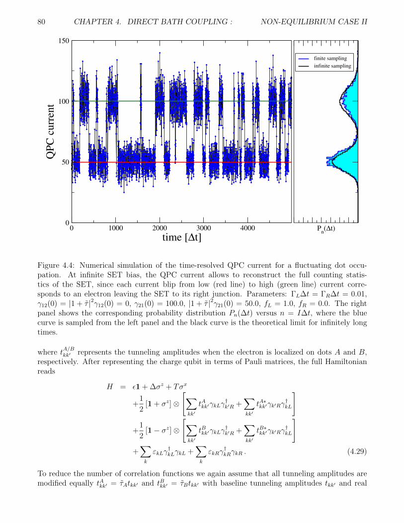
80 CHAPTER 4. DIRECT BATH COUPLING : NON-EQUILIBRIUM CASE II
0 1000 2000 3000 4000
time [∆t]
0
50
100
150
QP
C c
urr
ent
Pn(∆t)
finite sampling
infinite sampling
Figure 4.4: Numerical simulation of the time-resolved QPC current for a fluctuating dot occu-pation. At infinite SET bias, the QPC current allows to reconstruct the full counting statis-tics of the SET, since each current blip from low (red line) to high (green line) current corre-sponds to an electron leaving the SET to its right junction. Parameters: ΓL∆t = ΓR∆t = 0.01,γ12(0) = |1 + τ |2γ12(0) = 0, γ21(0) = 100.0, |1 + τ |2γ21(0) = 50.0, fL = 1.0, fR = 0.0. The rightpanel shows the corresponding probability distribution Pn(∆t) versus n = I∆t, where the bluecurve is sampled from the left panel and the black curve is the theoretical limit for infinitely longtimes.
where tA/Bkk′ represents the tunneling amplitudes when the electron is localized on dots A and B,
respectively. After representing the charge qubit in terms of Pauli matrices, the full Hamiltonianreads
H = ε1 + ∆σz + Tσx
+1
2[1 + σz]⊗
[∑kk′
tAkk′γkLγ†k′R +
∑kk′
tA∗kk′γk′Rγ†kL
]
+1
2[1− σz]⊗
[∑kk′
tBkk′γkLγ†k′R +
∑kk′
tB∗kk′γk′Rγ†kL
]+∑k
εkLγ†kLγkL +
∑k
εkRγ†kRγkR . (4.29)
To reduce the number of correlation functions we again assume that all tunneling amplitudes aremodified equally tAkk′ = τAtkk′ and tBkk′ = τBtkk′ with baseline tunneling amplitudes tkk′ and real
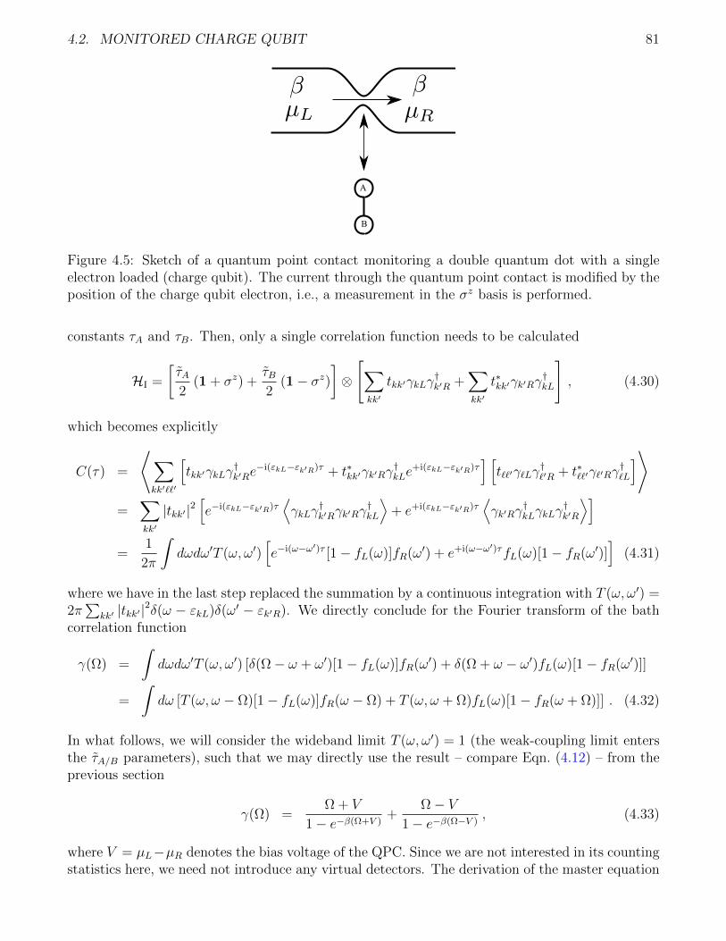
4.2. MONITORED CHARGE QUBIT 81
A
B
Figure 4.5: Sketch of a quantum point contact monitoring a double quantum dot with a singleelectron loaded (charge qubit). The current through the quantum point contact is modified by theposition of the charge qubit electron, i.e., a measurement in the σz basis is performed.
constants τA and τB. Then, only a single correlation function needs to be calculated
HI =
[τA2
(1 + σz) +τB2
(1− σz)]⊗
[∑kk′
tkk′γkLγ†k′R +
∑kk′
t∗kk′γk′Rγ†kL
], (4.30)
which becomes explicitly
C(τ) =
⟨∑kk′``′
[tkk′γkLγ
†k′Re
−i(εkL−εk′R)τ + t∗kk′γk′Rγ†kLe
+i(εkL−εk′R)τ] [t``′γ`Lγ
†`′R + t∗``′γ`′Rγ
†`L
]⟩=
∑kk′
|tkk′|2[e−i(εkL−εk′R)τ
⟨γkLγ
†k′Rγk′Rγ
†kL
⟩+ e+i(εkL−εk′R)τ
⟨γk′Rγ
†kLγkLγ
†k′R
⟩]=
1
2π
∫dωdω′T (ω, ω′)
[e−i(ω−ω′)τ [1− fL(ω)]fR(ω′) + e+i(ω−ω′)τfL(ω)[1− fR(ω′)]
](4.31)
where we have in the last step replaced the summation by a continuous integration with T (ω, ω′) =2π∑
kk′ |tkk′|2δ(ω − εkL)δ(ω′ − εk′R). We directly conclude for the Fourier transform of the bath
correlation function
γ(Ω) =
∫dωdω′T (ω, ω′) [δ(Ω− ω + ω′)[1− fL(ω)]fR(ω′) + δ(Ω + ω − ω′)fL(ω)[1− fR(ω′)]]
=
∫dω [T (ω, ω − Ω)[1− fL(ω)]fR(ω − Ω) + T (ω, ω + Ω)fL(ω)[1− fR(ω + Ω)]] . (4.32)
In what follows, we will consider the wideband limit T (ω, ω′) = 1 (the weak-coupling limit entersthe τA/B parameters), such that we may directly use the result – compare Eqn. (4.12) – from theprevious section
γ(Ω) =Ω + V
1− e−β(Ω+V )+
Ω− V1− e−β(Ω−V )
, (4.33)
where V = µL−µR denotes the bias voltage of the QPC. Since we are not interested in its countingstatistics here, we need not introduce any virtual detectors. The derivation of the master equation
82 CHAPTER 4. DIRECT BATH COUPLING : NON-EQUILIBRIUM CASE II
in the system energy eigenbasis requires diagonalization of the system Hamiltonian first – compareEq. (2.69)
E− = ε−√
∆2 + T 2 , |−〉 =∆−
√∆2 + T 2 |0〉+ T |1〉√
T 2 +(∆−
√∆2 + T 2
)2
E+ = ε+√
∆2 + T 2 , |+〉 =∆ +
√∆2 + T 2 |0〉+ T |1〉√
T 2 +(∆ +
√∆2 + T 2
)2. (4.34)
Following the Born-, Markov-, and secular approximations – compare definition 8 – we obtain aLindblad Master equation for the qubit
ρ = −i [HS +HLS, ρ] +∑abcd
γab,cd
[|a〉 〈b| ρ (|c〉 〈d|)† − 1
2
(|c〉 〈d|)† |a〉 〈b| , ρ
], (4.35)
where the summation only goes over the two energy eigenstates and HLS denotes the frequencyrenormalization. Since the two eigenvalues of our system are non-degenerate, the Lamb-shiftHamiltonian is diagonal in the system energy eigenbasis and does not affect the dynamics of thepopulations. In particular, we have for the populations the rate equation(
ρ−−ρ++
)=
(−γ+−,+− +γ−+,−+
+γ+−,+− −γ−+,−+
)(ρ−−ρ++
). (4.36)
The required dampening coefficients read
γ−+,−+ = γ(E+ − E−)|〈−|A |+〉|2 = γ(+2√
∆2 + T 2)T 2
4(∆2 + T 2)(τA − τB)2 ,
γ+−,+− = γ(E− − E+)|〈+|A |−〉|2 = γ(−2√
∆2 + T 2)T 2
4(∆2 + T 2)(τA − τB)2 . (4.37)
Exercise 42 (Qubit Dissipation) (1 points)Show the validity of Eqns. (4.37).
This shows that when the QPC current is not dependent on the qubit state τA = τB, the dissipa-tion on the qubit vanishes completely, which is consistent with our initial interaction Hamiltonian.In addition, in the pure dephasing limit T → 0, we do not have any dissipative back-action of themeasurement device on the qubit. Equation (4.36) obviously also preserves the trace of the densitymatrix. The stationary density matrix is therefore defined by
ρ++
ρ−−=γ+−,+−
γ−+,−+
=γ(−2
√∆2 + T 2)
γ(+2√
∆2 + T 2). (4.38)
When the QPC bias voltage vanishes (at equilibrium), we have
γ(−2√
∆2 + T 2)
γ(+2√
∆2 + T 2)→ e−β2
√∆2+T 2
= e−β(E+−E−) , (4.39)
4.2. MONITORED CHARGE QUBIT 83
i.e., the qubit thermalizes with the temperature of the QPC. When the QPC bias voltage is large,the qubit is driven away from this thermal state.
The evolution of coherences decouples from the diagonal elements of the density matrix. Thehermiticity of the density matrix allows to consider only one coherence
ρ−+ = −i (E− + ∆E− − E+ −∆E+) ρ−+
+
[γ−−,++ −
1
2(γ−−,−− + γ++,++ + γ−+,−+ + γ+−,+−)
]ρ−+ , (4.40)
where ∆E± corresponds to the energy renormalization due to the Lamb-shift, which induces afrequency renormalization of the qubit. The real part of the above equation is responsible for thedampening of the coherence, its calculation requires the evaluation of all remaining nonvanishingdampening coefficients
γ−+,−+ + γ+−,+− =[γ(+2
√∆2 + T 2) + γ(−2
√∆2 + T 2)
] T 2
4(T 2 + ∆2)(τA − τB)2 ,
γ−−,−− + γ++,++ − 2γ−−,++ = γ(0)∆2
T 2 + ∆2(τA − τB)2 . (4.41)
Using the decomposition of the dampening, we may now calculate the decoherence rate σ
σ = (γ−+,−+ + γ+−,+−) + (γ−−,−− + γ++,++ − 2γ−−,++)
=(τA − τB)2
4
T 2
∆2 + T 2
(V + 2
√∆2 + T 2
)coth
[β
2
(V + 2
√∆2 + T 2
)]+(V − 2
√∆2 + T 2
)coth
[β
2
(V − 2
√∆2 + T 2
)]+ (τA − τB)2 ∆2
∆2 + T 2V coth
[βV
2
], (4.42)
which vanishes as reasonably expected when we set τA = τB. Noting that x coth(x) ≥ 1 does notonly prove its positivity (i.e., the coherences always decay) but also enables one to obtain a roughlower bound
σ ≥ (τA − τB)2
β
T 2 + 2∆2
T 2 + ∆2(4.43)
on the dephasing rate. This lower bound is valid when the QPC voltage is rather small. For largevoltages |V |
√∆2 + T 2, the dephasing rate is given by
σ ≈ (τA − τB)2 T2 + 2∆2
T 2 + ∆2|V | (4.44)
and thus is limited by the voltage rather than the temperature.

84 CHAPTER 4. DIRECT BATH COUPLING : NON-EQUILIBRIUM CASE II
Chapter 5
Controlled systems:Non-Equilibrium Case III
Time-dependent equations of the form
ρ = L(t)ρ(t) (5.1)
are notoriously difficult to solve unless L(t) fulfills special properties.
• One such special case is e.g. the case of commuting superoperators, where the solution canbe obtained from the exponential of an integral
[L(t),L(t′)] = 0 =⇒ ρ(t) = exp
(−i
∫ t
0
L(t′)dt′)ρ0 . (5.2)
• Another special case is one with a very slow time-dependence and a unique stationary stateL(t)ρt = 0, where the time-dependent density matrix can be assumed to adiabatically followthe stationary state ρ(t) ≈ ρt.
• For fast time-dependencies, there exists the analytically solvable case of a train of δ-kicks
L(t) = L0 +∞∑i=1
`iδ(t− ti) , (5.3)
where the solution reads (tn < t < tn+1)
ρ(t) = eL0(t−tn)[e`neL0(tn−tn−1)
]× . . .×
[e`2eL0(t2−t1)
] [e`1eL0(t1)
]ρ0 , (5.4)
which can be considerably simplified using e.g. Baker-Campbell-Haussdorff relations whenthe kicks `i = ` and the timesteps tn − tn−1 = ∆t are identical.
• For periodic time-dependencies, Floquet theory may be applicable.
• Finally, a very simple case arises for piecewise-constant time-dependencies. This allows tomap the problem to ordinary differential equations with constant coefficients, which areevolved a certain amount of time. After an instantaneous switch of the coefficients, onesimply has initial conditions taken from the final state of the last evolution period, whichcan be evolved further and so on. Since it does not require an extension of the theoreticalframework, we will consider this case in the following.
85
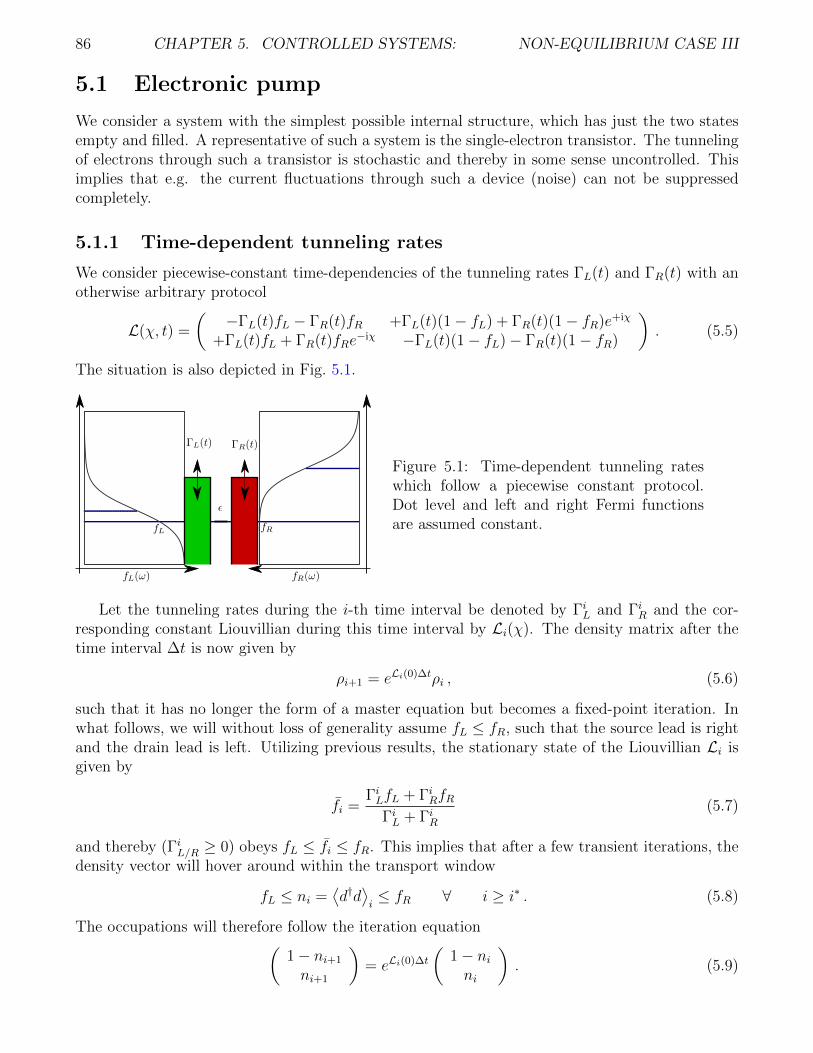
86 CHAPTER 5. CONTROLLED SYSTEMS: NON-EQUILIBRIUM CASE III
5.1 Electronic pump
We consider a system with the simplest possible internal structure, which has just the two statesempty and filled. A representative of such a system is the single-electron transistor. The tunnelingof electrons through such a transistor is stochastic and thereby in some sense uncontrolled. Thisimplies that e.g. the current fluctuations through such a device (noise) can not be suppressedcompletely.
5.1.1 Time-dependent tunneling rates
We consider piecewise-constant time-dependencies of the tunneling rates ΓL(t) and ΓR(t) with anotherwise arbitrary protocol
L(χ, t) =
(−ΓL(t)fL − ΓR(t)fR +ΓL(t)(1− fL) + ΓR(t)(1− fR)e+iχ
+ΓL(t)fL + ΓR(t)fRe−iχ −ΓL(t)(1− fL)− ΓR(t)(1− fR)
). (5.5)
The situation is also depicted in Fig. 5.1.
Figure 5.1: Time-dependent tunneling rateswhich follow a piecewise constant protocol.Dot level and left and right Fermi functionsare assumed constant.
Let the tunneling rates during the i-th time interval be denoted by ΓiL and ΓiR and the cor-responding constant Liouvillian during this time interval by Li(χ). The density matrix after thetime interval ∆t is now given by
ρi+1 = eLi(0)∆tρi , (5.6)
such that it has no longer the form of a master equation but becomes a fixed-point iteration. Inwhat follows, we will without loss of generality assume fL ≤ fR, such that the source lead is rightand the drain lead is left. Utilizing previous results, the stationary state of the Liouvillian Li isgiven by
fi =ΓiLfL + ΓiRfR
ΓiL + ΓiR(5.7)
and thereby (ΓiL/R ≥ 0) obeys fL ≤ fi ≤ fR. This implies that after a few transient iterations, thedensity vector will hover around within the transport window
fL ≤ ni =⟨d†d⟩i≤ fR ∀ i ≥ i∗ . (5.8)
The occupations will therefore follow the iteration equation(1− ni+1
ni+1
)= eLi(0)∆t
(1− nini
). (5.9)
5.1. ELECTRONIC PUMP 87
To calculate the number of particles tunneling into the source reservoir, we consider the moment-generating function
Mi(χ,∆t) = Tr
eLi(χ)∆t
(1− nini
)(5.10)
and calculate the first moment
〈n〉i = (−i)∂χMi(χ,∆t)|χ=0
=1
(ΓiL + ΓiR)2
[− (ΓiR)2(fR − ni)
(1− e−(ΓiL+ΓiR)∆t
)+ΓiLΓiR
((ni − fL)
(1− e−(ΓiL+ΓiR)∆t
)− (fR − fL)(ΓiL + ΓiR)∆t
) ]≤ 0 . (5.11)
Exercise 43 (Pumping Failure) (1 points)Show that under the assumption fL ≤ ni ≤ fR – and of course (ΓiL + ΓiR)∆t > 0 – the averagenumber of electrons travelling from left to right in Eq. (5.11) is always negative.
It follows that the average current always points from source to drain (in our case, sincefR > fL, from right to left), regardless of the actual protocol ΓαL/R chosen. Since any general
time-dependence Γα(t) can be approximated by piecewise-constant ones, we conclude that withsimply modifying the tunneling rates, it is not possible to revert the direction of the current.From a thermodynamic perspective, this is reasonable, since by changing the rates Γα(t) we donot inject energy into the system, and thus should not expect to get anything out of it. Note forlater reference however that this implies that the driving does not depend on whether the dot isoccupied or not, i.e., the rates are modified unconditionally (open-loop control).
5.1.2 With performing work
To revert the direction of transport, one could modify the Fermi functions e.g. by changing thechemical potentials or temperatures in the contacts. However, this first possibility may for fastdriving destroy the thermal equilibrium in the contacts, such that the whole approach might notbe applicable. Second, this approach would simply exchange the roles of source and drain, and apump that manages to pump water from a well into a bucket by lifting the complete lake facespoor economic perspectives.
Consequently, we consider changing the dot level ε(t) to change the value of the Fermi functions.Intuitively, it is quite straightforward to arrive at a protocol ε(t) and Γα(t) that should lift electronsfrom left to right and thereby pumps electrons from low to high chemical potentials, see Fig. 5.2.The Liouvillians for the first and second half cycles read
L1(χ) =
(−Γmax
L fL(εmin)− ΓminR fR(εmin) +Γmax
L [1− fL(εmin)] + ΓminR [1− fR(εmin)]e+iχ
+ΓmaxL fL(εmin) + Γmin
R fR(εmin)e−iχ −ΓmaxL [1− fL(εmin)]− Γmin
R [1− fR(εmin)]
),
L2(χ) =
(−Γmin
L fL(εmax)− ΓmaxR fR(εmax) +Γmin
L [1− fL(εmax)] + ΓmaxR [1− fR(εmax)]e+iχ
+ΓminL fL(εmax) + Γmax
R fR(εmax)e−iχ −ΓminL [1− fL(εmax)]− Γmax
R [1− fR(εmax)]
),
(5.12)
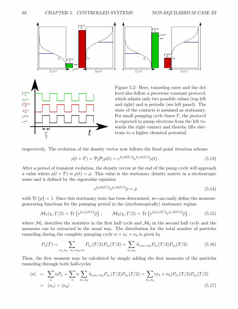
88 CHAPTER 5. CONTROLLED SYSTEMS: NON-EQUILIBRIUM CASE III
Figure 5.2: Here, tunneling rates and the dotlevel also follow a piecewise constant protocol,which admits only two possible values (top leftand right) and is periodic (see left panel). Thestate of the contacts is assumed as stationary.For small pumping cycle times T , the protocolis expected to pump electrons from the left to-wards the right contact and thereby lifts elec-trons to a higher chemical potential.
respectively. The evolution of the density vector now follows the fixed point iteration scheme
ρ(t+ T ) = P2P1ρ(t) = eL2(0)T/2eL1(0)T/2ρ(t) . (5.13)
After a period of transient evolution, the density vector at the end of the pump cycle will approacha value where ρ(t + T ) ≈ ρ(t) = ρ. This value is the stationary density matrix in a stroboscopicsense and is defined by the eigenvalue equation
eL2(0)T/2eL1(0)T/2ρ = ρ (5.14)
with Tr ρ = 1. Once this stationary state has been determined, we can easily define the moment-generating functions for the pumping period in the (stroboscopically) stationary regime
M1(χ, T/2) = TreL1(χ)T/2ρ
, M2(χ, T/2) = Tr
eL2(χ)T/2eL1(0)T/2ρ
, (5.15)
where M1 describes the statistics in the first half cycle and M2 in the second half cycle and themoments can be extracted in the usual way. The distribution for the total number of particlestunneling during the complete pumping cycle n = n1 + n2 is given by
Pn(T ) =∑
n1,n2 : n1+n2=n
Pn1(T/2)Pn2(T/2) =∑n1,n2
δn,n1+n2Pn1(T/2)Pn2(T/2) . (5.16)
Then, the first moment may be calculated by simply adding the first moments of the particlestunneling through both half-cycles
〈n〉 =∑n
nPn =∑n
n∑n1,n2
δn,n1+n2Pn1(T/2)Pn2(T/2) =∑n1,n2
(n1 + n2)Pn1(T/2)Pn2(T/2)
= 〈n1〉+ 〈n2〉 . (5.17)
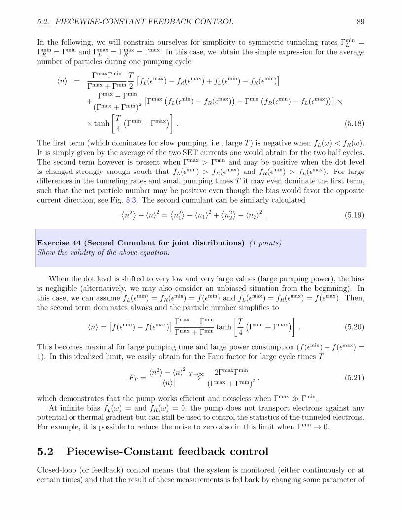
5.2. PIECEWISE-CONSTANT FEEDBACK CONTROL 89
In the following, we will constrain ourselves for simplicity to symmetric tunneling rates ΓminL =
ΓminR = Γmin and Γmax
L = ΓmaxR = Γmax. In this case, we obtain the simple expression for the average
number of particles during one pumping cycle
〈n〉 =ΓmaxΓmin
Γmax + Γmin
T
2
[fL(εmax)− fR(εmax) + fL(εmin)− fR(εmin)
]+
Γmax − Γmin
(Γmax + Γmin)2
[Γmax
(fL(εmin)− fR(εmax)
)+ Γmin
(fR(εmin)− fL(εmax)
)]×
× tanh
[T
4
(Γmin + Γmax
)]. (5.18)
The first term (which dominates for slow pumping, i.e., large T ) is negative when fL(ω) < fR(ω).It is simply given by the average of the two SET currents one would obtain for the two half cycles.The second term however is present when Γmax > Γmin and may be positive when the dot levelis changed strongly enough souch that fL(εmin) > fR(εmax) and fR(εmin) > fL(εmax). For largedifferences in the tunneling rates and small pumping times T it may even dominate the first term,such that the net particle number may be positive even though the bias would favor the oppositecurrent direction, see Fig. 5.3. The second cumulant can be similarly calculated⟨
n2⟩− 〈n〉2 =
⟨n2
1
⟩− 〈n1〉2 +
⟨n2
2
⟩− 〈n2〉2 . (5.19)
Exercise 44 (Second Cumulant for joint distributions) (1 points)Show the validity of the above equation.
When the dot level is shifted to very low and very large values (large pumping power), the biasis negligible (alternatively, we may also consider an unbiased situation from the beginning). Inthis case, we can assume fL(εmin) = fR(εmin) = f(εmin) and fL(εmax) = fR(εmax) = f(εmax). Then,the second term dominates always and the particle number simplifies to
〈n〉 =[f(εmin)− f(εmax)
] Γmax − Γmin
Γmax + Γmintanh
[T
4
(Γmin + Γmax
)]. (5.20)
This becomes maximal for large pumping time and large power consumption (f(εmin)− f(εmax) =1). In this idealized limit, we easily obtain for the Fano factor for large cycle times T
FT =〈n2〉 − 〈n〉2
|〈n〉|T→∞→ 2ΓmaxΓmin
(Γmax + Γmin)2 , (5.21)
which demonstrates that the pump works efficient and noiseless when Γmax Γmin.At infinite bias fL(ω) = and fR(ω) = 0, the pump does not transport electrons against any
potential or thermal gradient but can still be used to control the statistics of the tunneled electrons.For example, it is possible to reduce the noise to zero also in this limit when Γmin → 0.
5.2 Piecewise-Constant feedback control
Closed-loop (or feedback) control means that the system is monitored (either continuously or atcertain times) and that the result of these measurements is fed back by changing some parameter of
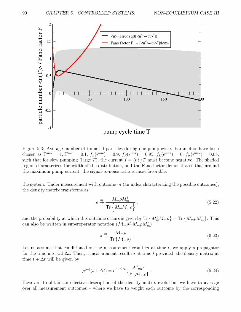
90 CHAPTER 5. CONTROLLED SYSTEMS: NON-EQUILIBRIUM CASE III
50 100 150 200
pump cycle time T-1
-0,5
0
0,5
1
1,5
2
par
ticl
e n
um
ber
<n
(T)>
/ F
ano
fac
tor
F<n> (error sqrt[<n
2>-<n>
2])
Fano factor FT = [<n
2>-<n>
2]/|<n>|
Figure 5.3: Average number of tunneled particles during one pump cycle. Parameters have beenchosen as Γmax = 1, Γmin = 0.1, fL(εmin) = 0.9, fR(εmin) = 0.95, fL(εmax) = 0, fR(εmax) = 0.05,such that for slow pumping (large T ), the current I = 〈n〉 /T must become negative. The shadedregion characterizes the width of the distribution, and the Fano factor demonstrates that aroundthe maximum pump current, the signal-to-noise ratio is most favorable.
the system. Under measurement with outcome m (an index characterizing the possible outcomes),the density matrix transforms as
ρm→ MmρM
†m
TrM †
mMmρ , (5.22)
and the probability at which this outcome occurs is given by TrM †
mMmρ
= TrMmρM
†m
. This
can also be written in superoperator notation (Mmρ=MmρM†m)
ρm→ Mmρ
Tr Mmρ. (5.23)
Let us assume that conditioned on the measurement result m at time t, we apply a propagatorfor the time interval ∆t. Then, a measurement result m at time t provided, the density matrix attime t+ ∆t will be given by
ρ(m)(t+ ∆t) = eL(m)∆t Mmρ
Tr Mmρ. (5.24)
However, to obtain an effective description of the density matrix evolution, we have to averageover all measurement outcomes – where we have to weight each outcome by the corresponding
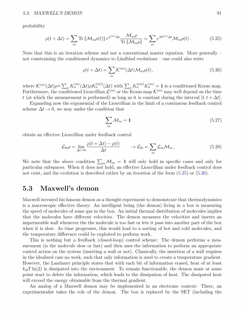
5.3. MAXWELL’S DEMON 91
probability
ρ(t+ ∆t) =∑m
Tr Mmρ(t) eL(m)∆t Mmρ
Tr Mmρ=∑m
eM(m)∆tMmρ(t) . (5.25)
Note that this is an iteration scheme and not a conventional master equation. More generally –not constraining the conditioned dynamics to Lindblad evolutions – one could also write
ρ(t+ ∆t) =∑m
K(m)(∆t)Mmρ(t) , (5.26)
where K(m)(∆t)ρ=∑
αK(m)α (∆t)ρK
(m)†α (∆t) with
∑αK
(m)†α K
(m)α = 1 is a conditioned Kraus map.
Furthermore, the conditioned Liouvillian L(m) or the Kraus map K(m) may well depend on the timet (at which the measurement is performed) as long as it is constant during the interval [t, t+ ∆t].
Expanding now the exponential of the Liouvillian in the limit of a continuous feedback controlscheme ∆t→ 0, we may under the condition that∑
m
Mm = 1 (5.27)
obtain an effective Liouvillian under feedback control
Lfbρ = lim∆t→0
ρ(t+ ∆t)− ρ(t)
∆t→ Lfb =
∑m
LmMm . (5.28)
We note that the above condition∑
mMm = 1 will only hold in specific cases and only forparticular subspaces. When it does not hold, an effective Liouvillian under feedback control doesnot exist, and the evolution is described rather by an iteration of the form (5.25) or (5.26).
5.3 Maxwell’s demon
Maxwell invented his famous demon as a thought experiment to demonstrate that thermodynamicsis a macroscopic effective theory: An intelligent being (the demon) living in a box is measuringthe speed of molecules of some gas in the box. An initial thermal distribution of molecules impliesthat the molecules have different velocities. The demon measures the velocities and inserts animpermeable wall whenever the the molecule is too fast or lets it pass into another part of the boxwhen it is slow. As time progresses, this would lead to a sorting of hot and cold molecules, andthe temperature difference could be exploited to perform work.
This is nothing but a feedback (closed-loop) control scheme: The demon performs a mea-surement (is the molecule slow or fast) and then uses the information to perform an appropriatecontrol action on the system (inserting a wall or not). Classically, the insertion of a wall requiresin the idealized case no work, such that only information is used to create a temperature gradient.However, the Landauer principle states that with each bit of information erased, heat of at leastkBT ln(2) is dissipated into the environment. To remain functionable, the demon must at somepoint start to delete the information, which leads to the dissipation of heat. The dissipated heatwill exceed the energy obtainable from the thermal gradient.
An analog of a Maxwell demon may be implemented in an electronic context: There, anexperimentalist takes the role of the demon. The box is replaced by the SET (including the
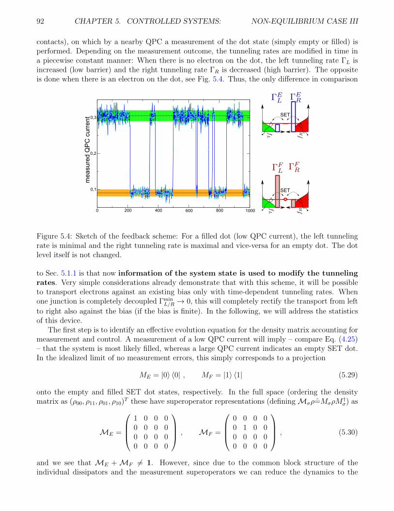
92 CHAPTER 5. CONTROLLED SYSTEMS: NON-EQUILIBRIUM CASE III
contacts), on which by a nearby QPC a measurement of the dot state (simply empty or filled) isperformed. Depending on the measurement outcome, the tunneling rates are modified in time ina piecewise constant manner: When there is no electron on the dot, the left tunneling rate ΓL isincreased (low barrier) and the right tunneling rate ΓR is decreased (high barrier). The oppositeis done when there is an electron on the dot, see Fig. 5.4. Thus, the only difference in comparison
0 200 400 600 800 1000
0,1
0,2
0,3
me
asu
red
QP
C c
urr
en
t SET
SET
Figure 5.4: Sketch of the feedback scheme: For a filled dot (low QPC current), the left tunnelingrate is minimal and the right tunneling rate is maximal and vice-versa for an empty dot. The dotlevel itself is not changed.
to Sec. 5.1.1 is that now information of the system state is used to modify the tunnelingrates. Very simple considerations already demonstrate that with this scheme, it will be possibleto transport electrons against an existing bias only with time-dependent tunneling rates. Whenone junction is completely decoupled Γmin
L/R → 0, this will completely rectify the transport from left
to right also against the bias (if the bias is finite). In the following, we will address the statisticsof this device.
The first step is to identify an effective evolution equation for the density matrix accounting formeasurement and control. A measurement of a low QPC current will imply – compare Eq. (4.25)– that the system is most likely filled, whereas a large QPC current indicates an empty SET dot.In the idealized limit of no measurement errors, this simply corresponds to a projection
ME = |0〉 〈0| , MF = |1〉 〈1| (5.29)
onto the empty and filled SET dot states, respectively. In the full space (ordering the densitymatrix as (ρ00, ρ11, ρ01, ρ10)T these have superoperator representations (definingMσρ=MσρM
†σ) as
ME =
1 0 0 00 0 0 00 0 0 00 0 0 0
, MF =
0 0 0 00 1 0 00 0 0 00 0 0 0
, (5.30)
and we see that ME +MF 6= 1. However, since due to the common block structure of theindividual dissipators and the measurement superoperators we can reduce the dynamics to the
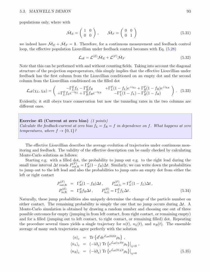
5.3. MAXWELL’S DEMON 93
populations only, where with
ME =
(1 00 0
), MF =
(0 00 1
)(5.31)
we indeed have ME + MF = 1. Therefore, for a continuous measurement and feedback controlloop, the effective population Liouvillian under feedback control becomes with Eq. (5.28)
Leff = L(E)ME + L(F )MF (5.32)
Note that this can be performed with and without counting fields. Taking into account the diagonalstructure of the projection superoperators, this simply implies that the effective Liouvillian underfeedback has the first column from the Liouvillian conditioned on an empty dot and the secondcolumn from the Liouvillian conditioned on the filled dot
Leff(χL, χR) =
(−ΓELfL − ΓERfR +ΓFL(1− fL)e+iχL + ΓFR(1− fR)e+iχR
+ΓELfLe−iχL + ΓERfRe
−iχR −ΓFL(1− fL)− ΓFR(1− fR)
). (5.33)
Evidently, it still obeys trace conservation but now the tunneling rates in the two columns aredifferent ones.
Exercise 45 (Current at zero bias) (1 points)Calculate the feedback-current at zero bias fL = fR = f in dependence on f . What happens at zerotemperatures, where f → 0, 1?
The effective Liouvillian describes the average evolution of trajectories under continuous mon-itoring and feedback. The validity of the effective description can be easily checked by calculatingMonte-Carlo solutions as follows:
Starting e.g. with a filled dot, the probability to jump out e.g. to the right lead during thesmall time interval ∆t reads P
(F )out,R = ΓFR(1−fR)∆t. Similarly, we can write down the probabilities
to jump out to the left lead and also the probabilities to jump onto an empty dot from either theleft or right contact
P(F )out,R = ΓFR(1− fR)∆t , P
(F )out,L = ΓFL(1− fL)∆t ,
P(E)in,R = ΓERfR∆t , P
(E)in,L = ΓELfL∆t . (5.34)
Naturally, these jump probabilities also uniquely determine the change of the particle number oneither contact. The remaining probability is simply the one that no jump occurs during ∆t. AMonte-Carlo simulation is obtained by drawing a random number and choosing one out of threepossible outcomes for empty (jumping in from left contact, from right contact, or remaining empty)and for a filled (jumping out to left contact, to right contact, or remaining filled) dot. Repeatingthe procedure several times yields a single trajectory for n(t), nL(t), and nR(t). The ensembleaverage of many such trajectories agree perfectly with the solution
〈n〉t = Trd†deLeff(0,0)tρ0
,
〈nL〉t = (−i∂χ) TreLeff(χ,0)tρ0
∣∣χ=0
,
〈nR〉t = (−i∂χ) TreLeff(0,χ)tρ0
∣∣χ=0
(5.35)
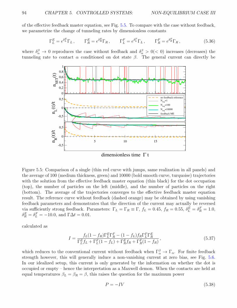
94 CHAPTER 5. CONTROLLED SYSTEMS: NON-EQUILIBRIUM CASE III
of the effective feedback master equation, see Fig. 5.5. To compare with the case without feedback,we parametrize the change of tunneling rates by dimensionless constants
ΓEL = eδELΓL , ΓER = eδ
ERΓR , ΓFL = eδ
FLΓL , ΓFR = eδ
FRΓR , (5.36)
where δβα → 0 reproduces the case without feedback and δβα > 0(< 0) increases (decreases) thetunneling rate to contact α conditioned on dot state β. The general current can directly be
0
0,2
0,4
0,6
0,8
1
nS
ET(t
)
-0,5
0
0,5
nL(t
)/t
5 10 15
dimensionless time Γ t
-0,5
0
0,5
nR(t
)/t
no feedback reference
Ntraj
=1
Ntraj
=100
Ntraj
=10000
feedback ME
Figure 5.5: Comparison of a single (thin red curve with jumps, same realization in all panels) andthe average of 100 (medium thickness, green) and 10000 (bold smooth curve, turquoise) trajectorieswith the solution from the effective feedback master equation (thin black) for the dot occupation(top), the number of particles on the left (middle), and the number of particles on the right(bottom). The average of the trajectories converges to the effective feedback master equationresult. The reference curve without feedback (dashed orange) may be obtained by using vanishingfeedback parameters and demonstrates that the direction of the current may actually be reversedvia sufficiently strong feedback. Parameters: ΓL = ΓR ≡ Γ, fL = 0.45, fR = 0.55, δEL = δFR = 1.0,δER = δFL = −10.0, and Γ∆t = 0.01.
calculated as
I =fL(1− fR)ΓELΓFR − (1− fL)fRΓFLΓER
ΓELfL + ΓFL(1− fL) + ΓERfR + ΓFR(1− fR), (5.37)
which reduces to the conventional current without feedback when Γβα → Γα. For finite feedbackstrength however, this will generally induce a non-vanishing current at zero bias, see Fig. 5.6.In our idealized setup, this current is only generated by the information on whether the dot isoccupied or empty – hence the interpretation as a Maxwell demon. When the contacts are held atequal temperatures βL = βR = β, this raises the question for the maximum power
P = −IV (5.38)
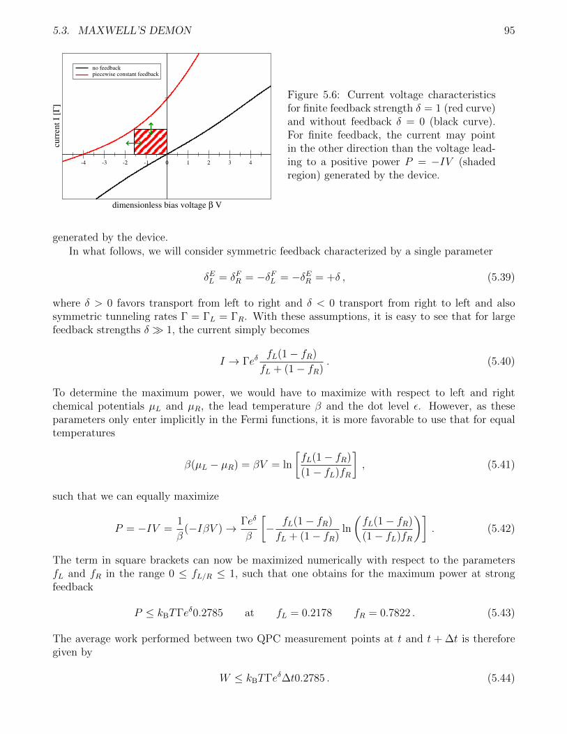
5.3. MAXWELL’S DEMON 95
-4 -3 -2 -1 0 1 2 3 4
dimensionless bias voltage β V
curr
ent
I [Γ
]
no feedbackpiecewise constant feedback
Figure 5.6: Current voltage characteristicsfor finite feedback strength δ = 1 (red curve)and without feedback δ = 0 (black curve).For finite feedback, the current may pointin the other direction than the voltage lead-ing to a positive power P = −IV (shadedregion) generated by the device.
generated by the device.In what follows, we will consider symmetric feedback characterized by a single parameter
δEL = δFR = −δFL = −δER = +δ , (5.39)
where δ > 0 favors transport from left to right and δ < 0 transport from right to left and alsosymmetric tunneling rates Γ = ΓL = ΓR. With these assumptions, it is easy to see that for largefeedback strengths δ 1, the current simply becomes
I → ΓeδfL(1− fR)
fL + (1− fR). (5.40)
To determine the maximum power, we would have to maximize with respect to left and rightchemical potentials µL and µR, the lead temperature β and the dot level ε. However, as theseparameters only enter implicitly in the Fermi functions, it is more favorable to use that for equaltemperatures
β(µL − µR) = βV = ln
[fL(1− fR)
(1− fL)fR
], (5.41)
such that we can equally maximize
P = −IV =1
β(−IβV )→ Γeδ
β
[− fL(1− fR)
fL + (1− fR)ln
(fL(1− fR)
(1− fL)fR
)]. (5.42)
The term in square brackets can now be maximized numerically with respect to the parametersfL and fR in the range 0 ≤ fL/R ≤ 1, such that one obtains for the maximum power at strongfeedback
P ≤ kBTΓeδ0.2785 at fL = 0.2178 fR = 0.7822 . (5.43)
The average work performed between two QPC measurement points at t and t + ∆t is thereforegiven by
W ≤ kBTΓeδ∆t0.2785 . (5.44)
96 CHAPTER 5. CONTROLLED SYSTEMS: NON-EQUILIBRIUM CASE III
However, to perform feedback efficiently, it is required that the QPC sampling rate is fast enoughthat all state changes of the SET are faithfully detected (no tunneling charges are missed). Thisrequires that Γeδ∆t < 1. Therefore, we can refine the upper bound for the average work
W ≤ kBT0.2785 . (5.45)
This has to be contrasted with the Landauer principle, which states that for each deleted bit inthe demons brain (each QPC data point enconding high current or low current) heat of
Q ≥ kBT ln(2) ≈ kBT0.6931 (5.46)
is dissipated. These rough estimates indicate that the second law does not appear to be violated.The conventional fluctuation theorem for the SET at equal temperatures
P+n(t)
P−n(t)= enβV (5.47)
is modified in presence of feedback. However, since the Liouvillian still contains the countingfields in the conventional way, simply the factor in the exponential, not the dependence on thenumber of tunneled electrons n is changed. To evaluate the FT, we identify symmetries in themoment-generating function (or alternatively the eigenvalues of the Liouvillian)
λ(−χ) = λ
(+χ+ i ln
[ΓELΓFRΓFLΓER
fL(1− fR)
(1− fL)fR
])= λ
(+χ+ i ln
[e+4δ fL(1− fR)
(1− fL)fR
])= λ
(+χ+ i ln
[e+4δeβV
])= λ(+χ+ i(4δ + βV )) . (5.48)
From this symmetry of the cumulant-generating function we obtain for the fluctuation theoremunder feedback
limt→∞
P+n(t)
P−n(t)= en(βV+4δ) = enβ(V−V ∗) , (5.49)
where V ∗ = −4δ/β denotes the voltage at which the current (under feedback) vanishes.In the exponential, we do no longer have the conventional entropy production that is in the
long-term limit essentially given by the heat transfer. Instead, the modification indicates that thesecond law must be modified by the information that is used to implement the control loop.
Exercise 46 (Vanishing feedback current) (1 points)Show for equal temperatures that the feedback current vanishes when V = V ∗ = −4δ/β.
The fact that the estimates concerning the second law are rather vague result from the missingphysical implementation of the control loop. In our model, it could be anything, even representedby a human being pressing a button whenever the QPC current changes. The entropy producedby such a humanoid implementation of the control loop would by far exceed the local entropyreduction manifested by a current running against the bias. Below, we discuss an all-inclusiveimplementation of the control loop, where we can answer these things quantitatively.
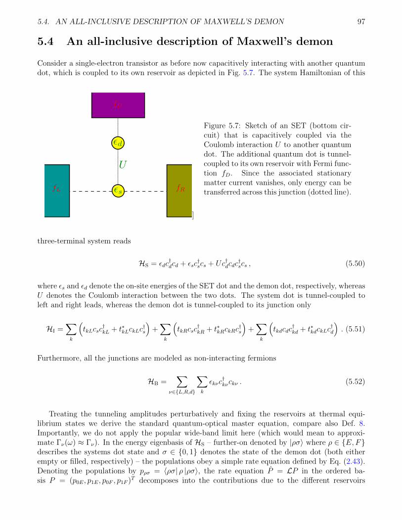
5.4. AN ALL-INCLUSIVE DESCRIPTION OF MAXWELL’S DEMON 97
5.4 An all-inclusive description of Maxwell’s demon
Consider a single-electron transistor as before now capacitively interacting with another quantumdot, which is coupled to its own reservoir as depicted in Fig. 5.7. The system Hamiltonian of this
]
Figure 5.7: Sketch of an SET (bottom cir-cuit) that is capacitively coupled via theCoulomb interaction U to another quantumdot. The additional quantum dot is tunnel-coupled to its own reservoir with Fermi func-tion fD. Since the associated stationarymatter current vanishes, only energy can betransferred across this junction (dotted line).
three-terminal system reads
HS = εdc†dcd + εsc
†scs + Uc†dcdc
†scs , (5.50)
where εs and εd denote the on-site energies of the SET dot and the demon dot, respectively, whereasU denotes the Coulomb interaction between the two dots. The system dot is tunnel-coupled toleft and right leads, whereas the demon dot is tunnel-coupled to its junction only
HI =∑k
(tkLcsc
†kL + t∗kLckLc
†s
)+∑k
(tkRcsc
†kR + t∗kRckRc
†s
)+∑k
(tkdcdc
†kd + t∗kdckLc
†d
). (5.51)
Furthermore, all the junctions are modeled as non-interacting fermions
HB =∑
ν∈L,R,d
∑k
εkνc†kνckν . (5.52)
Treating the tunneling amplitudes perturbatively and fixing the reservoirs at thermal equi-librium states we derive the standard quantum-optical master equation, compare also Def. 8.Importantly, we do not apply the popular wide-band limit here (which would mean to approxi-mate Γν(ω) ≈ Γν). In the energy eigenbasis of HS – further-on denoted by |ρσ〉 where ρ ∈ E,Fdescribes the systems dot state and σ ∈ 0, 1 denotes the state of the demon dot (both eitherempty or filled, respectively) – the populations obey a simple rate equation defined by Eq. (2.43).Denoting the populations by pρσ = 〈ρσ| ρ |ρσ〉, the rate equation P = LP in the ordered ba-sis P = (p0E, p1E, p0F , p1F )T decomposes into the contributions due to the different reservoirs
98 CHAPTER 5. CONTROLLED SYSTEMS: NON-EQUILIBRIUM CASE III
L = LD + LL + LR, which read
LD =
−ΓDfD +ΓD(1− fD) 0 0+ΓDfD −ΓD(1− fD) 0 0
0 0 −ΓUDfUD +ΓUD(1− fUD )
0 0 +ΓUDfUD −ΓUD(1− fUD )
,
Lα =
−Γαfα 0 +Γα(1− fα) 0
0 −ΓUαfUα 0 +ΓUα (1− fUα )
+Γαfα 0 −Γα(1− fα) 00 +ΓUαf
Uα 0 −ΓUα (1− fUα )
, α ∈ L,R , (5.53)
where we have used the abbreviations Γα = Γα(εs) and ΓUα = Γα(εs + U) for α ∈ L,R andΓD = ΓD(εd) and ΓUD = ΓD(εd + U) for the tunneling rates and similarly for the Fermi functionsfα = fα(εs), f
Uα = fα(εs + U), fD = fD(εd), and fUD = fD(εd + U), respectively. We note that
all contributions separately obey local-detailed balance relations. Closer inspection of the rates inEq. (5.53) reveals that these rates could have been guessed without any microscopic derivation.For example, the transition rate from state |1E〉 to state |0E〉 is just given by the bare tunnelingrate for the demon junction ΓD multiplied by the probability to find a free space in the terminal attransition frequency εd. Similarly, the transition rate from state |1F 〉 to state |0F 〉 corresponds toan electron jumping out of the demon dot to its junction, this time, however, transporting energyof εd +U . We have ordered our basis such that the upper left block of LD describes the dynamicsof the demon dot conditioned on an empty system dot, whereas the lower block accounts for thedynamics conditioned on a filled system.
As a whole, the system respects the second law of thermodynamics. We demonstrate this byanalyzing the entropy production by means of the Full Counting Statistics. In order to avoidhaving to trace six counting fields, we note that the system obeys three conservation laws, sincethe two dots may only exchange energy but not matter
I(L)M + I
(R)M = 0 , I
(D)M = 0 , I
(L)E + I
(R)E + I
(D)E = 0 , (5.54)
where I(ν)E and I
(ν)M denote energy and matter currents to terminal ν, respectively. Therefore,
three counting fields should in general suffice to completely track the entropy production in thelong-term limit. For simplicity however, we compute the entropy production for the more realisticcase of equal temperatures at the left and right SET junction β = βL = βR. Technically, this isconveniently performed by balancing with the entropy flow and using the conservation laws
Si = −Se = −∑ν
β(ν)(I(ν)E − µ
(ν)I(ν)M )
= −β(I(L)E − µLI(L)
M + I(R)E − µRI(R)
M )− βDI(D)E
= (β − βD)I(D)E − β(µL − µR)I
(R)M . (5.55)
Thus, we conclude that for equal temperatures left and right it should even suffice to track e.g.only the energy transferred to the demon junction and the particles to the right lead. Therefore,we introduce counting fields for the demon (ξ) and for the particles transferred to the left junctions
5.4. AN ALL-INCLUSIVE DESCRIPTION OF MAXWELL’S DEMON 99
(χ), and the counting-field dependent rate equation becomes
LD(ξ) =
−ΓDfD +ΓD(1− fD)e+iξεd 0 0
+ΓDfDe−iξεd −ΓD(1− fD) 0 0
0 0 −ΓUDfUD +ΓUD(1− fUD )e+iξ(εd+U)
0 0 +ΓUDfUDe−iξ(εd+U) −ΓUD(1− fUD )
,
LR(χ) =
−ΓRfR 0 +ΓR(1− fR)e+iχ 0
0 −ΓURfUR 0 +ΓUR(1− fUR )e+iχ
+ΓRfRe−iχ 0 −ΓR(1− fR) 0
0 +ΓURfUR e−iχ 0 −ΓUR(1− fUR )
. (5.56)
These counting fields can now be used to reconstruct the statistics of energy and matter transfer.The currents can be obtained by performing suitable derivatives of the rate matrix. For example,
the energy current to the demon is given by I(D)E = −iTr
∂ξL(ξ, 0)|ξ=0 ρ
, where ρ is the steady
state L(0, 0)ρ = 0.To test the fluctuation theorem, we calculate the characteristic polynomial
D(ξ, χ) = |L(ξ, χ)− λ1|= (L11 − λ)(L22 − λ)(L33 − λ)(L44 − λ)
−(L11 − λ)(L22 − λ)L34(ξ)L43(ξ)− (L11 − λ)(L33 − λ)L24(χ)L42(χ)
−(L22 − λ)(L44 − λ)L13(χ)L31(χ)− (L33 − λ)(L44 − λ)L12(ξ)L21(ξ)
+L12(ξ)L21(ξ)L34(ξ)L43(ξ) + L13(χ)L31(χ)L24(χ)L42(χ)
−L12(ξ)L24(χ)L31(χ)L43(ξ)− L13(χ)L21(ξ)L34(ξ)L42(χ)
= (L11 − λ)(L22 − λ)(L33 − λ)(L44 − λ)
−(L11 − λ)(L22 − λ)L34(0)L43(0)− (L11 − λ)(L33 − λ)L24(χ)L42(χ)
−(L22 − λ)(L44 − λ)L13(χ)L31(χ)− (L33 − λ)(L44 − λ)L12(0)L21(0)
+L12(0)L21(0)L34(0)L43(0) + L13(χ)L31(χ)L24(χ)L42(χ)
−L12(ξ)L24(χ)L31(χ)L43(ξ)− L13(χ)L21(ξ)L34(ξ)L42(χ) , (5.57)
where Lij simply denote the matrix elements of the rate matrix L. We note the symmetries
L13(−χ) =1− fLfL
L31
(+χ+ i ln
fL(1− fR)
(1− fL)fR
)=
1− fLfL
L31 (+χ+ iβ(µL − µR)) ,
L24(−χ) =1− fULfUL
L42
(+χ+ i ln
fUL (1− fUR )
(1− fUL )fUR
)=
1− fULfUL
L42 (+χ+ iβ(µL − µR)) ,
L12(−ξ) = L21
(+ξ +
i
εdln
1− fDfD
)= L21
(+ξ +
i
εdβD(εd − µD)
),
L34(−ξ) = L43
(+ξ +
i
εd + Uln
1− fUDfUD
)= L43
(+ξ +
i
εd + UβD(εd + U − µD)
), (5.58)
which can be used to show that the full characteristic polynomial obeys the symmetry
D(−ξ,−χ) = D(ξ + i(βD − β)/U, χ+ iβ(µL − µR)) . (5.59)
This symmetry implies – when monitoring the energy current to the demon eD and the number ofelectrons transferred to the right junction nR – for the corresponding probability distribution the
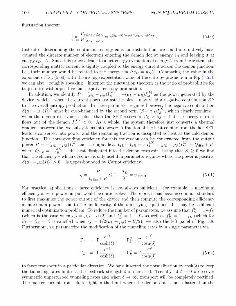
100 CHAPTER 5. CONTROLLED SYSTEMS: NON-EQUILIBRIUM CASE III
fluctuation theorem
limt→∞
P+∆nS ,+∆eD
P−∆nS ,−∆eD
= e(βD−β)∆eD+β(µL−µR)∆nS . (5.60)
Instead of determining the continuous energy emission distribution, we could alternatively havecounted the discrete number of electrons entering the demon dot at energy εD and leaving it atenergy εD+U . Since this process leads to a net energy extraction of energy U from the system, thecorresponding matter current is tightly coupled to the energy current across the demon junction,i.e., their number would be related to the energy via ∆eD = nDU . Comparing the value in theexponent of Eq. (5.60) with the average expectation value of the entropy production in Eq. (5.55),we can also – roughly speaking – interpret the fluctuation theorem as the ratio of probabilities fortrajectories with a positive and negative entropy production.
In addition, we identify P = (µL − µR)I(R)M = −(µL − µR)I
(L)M as the power generated by the
device, which – when the current flows against the bias – may yield a negative contribution βPto the overall entropy production. In these parameter regimes however, the negative contributionβ(µL − µR)I
(R)M must be over-balanced by the second term (β − βD)I
(D)E , which clearly requires –
when the demon reservoir is colder than the SET reservoirs βD > βS – that the energy currentflows out of the demon I
(D)E < 0. As a whole, the system therefore just converts a thermal
gradient between the two subsystems into power: A fraction of the heat coming from the hot SETleads is converted into power, and the remaining fraction is dissipated as heat at the cold demonjunction. The corresponding efficiency for this conversion can be constructed from the outputpower P = −(µL − µR)I
(L)M and the input heat QL + QR = −I(D)
E − (µL − µR)I(L)M = Qdiss + P ,
where Qdiss = −I(D)E is the heat dissipated into the demon reservoir. Using that Si ≥ 0 we find
that the efficiency – which of course is only useful in parameter regimes where the power is positiveβ(µL − µR)I
(R)M > 0 – is upper-bounded by Carnot efficiency
η =P
Qdiss + P≤ 1− TD
T= ηCarnot . (5.61)
For practical applications a large efficiency is not always sufficient. For example, a maximumefficiency at zero power output would be quite useless. Therefore, it has become common standardto first maximize the power output of the device and then compute the corresponding efficiencyat maximum power. Due to the nonlinearity of the underlying equations, this may be a difficultnumerical optimization problem. To reduce the number of parameters, we assume that fUD = 1−fD(which is the case when εD = µD − U/2) and fUL = 1 − fR as well as fUR = 1 − fL (which forβL = βR = β is satisfied when εS = 1/2(µL + µR) − U/2), see also the left panel of Fig. 5.8.Furthermore, we parametrize the modification of the tunneling rates by a single parameter via
ΓL = Γe+δ
cosh(δ), ΓUL = Γ
e−δ
cosh(δ)
ΓR = Γe−δ
cosh(δ), ΓUR = Γ
e+δ
cosh(δ)(5.62)
to favor transport in a particular direction. We have inserted the normalization by cosh(δ) to keepthe tunneling rates finite as the feedback strength δ is increased. Trivially, at δ = 0 we recoversymmetric unperturbed tunneling rates and when δ → ∞, transport will be completely rectified.The matter current from left to right in the limit where the demon dot is much faster than the
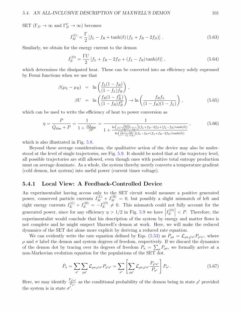
5.4. AN ALL-INCLUSIVE DESCRIPTION OF MAXWELL’S DEMON 101
SET (ΓD →∞ and ΓUD →∞) becomes
I(L)M =
Γ
2[fL − fR + tanh(δ) (fL + fR − 2fD)] . (5.63)
Similarly, we obtain for the energy current to the demon
I(D)E =
ΓU
2[fL + fR − 2fD + (fL − fR) tanh(δ)] , (5.64)
which determines the dissipated heat. These can be converted into an efficiency solely expressedby Fermi functions when we use that
β(µL − µR) = ln
(fL(1− fR)
(1− fL)fR
),
βU = ln
(fR(1− fUR )
(1− fR)fUR
)→ ln
(fRfL
(1− fR)(1− fL)
), (5.65)
which can be used to write the efficiency of heat to power conversion as
η =P
Qdiss + P=
1
1 + βQdiss
βP
=1
1 +ln(
fRfL(1−fR)(1−fL)
)(fL+fR−2fD+(fL−fR) tanh(δ))
ln(fL(1−fR)
(1−fL)fR
)(fL−fR+(fL+fR−2fD) tanh(δ))
, (5.66)
which is also illustrated in Fig. 5.8.Beyond these average considerations, the qualitative action of the device may also be under-
stood at the level of single trajectories, see Fig. 5.9. It should be noted that at the trajectory level,all possible trajectories are still allowed, even though ones with positive total entropy productionmust on average dominate. As a whole, the system thereby merely converts a temperature gradient(cold demon, hot system) into useful power (current times voltage).
5.4.1 Local View: A Feedback-Controlled Device
An experimentalist having access only to the SET circuit would measure a positive generatedpower, conserved particle currents I
(L)M + I
(R)M = 0, but possibly a slight mismatch of left and
right energy currents I(L)E + I
(R)E = −I(D)
E 6= 0. This mismatch could not fully account for the
generated power, since for any efficiency η > 1/2 in Fig. 5.9 we have∣∣∣I(D)E
∣∣∣ < P . Therefore, the
experimentalist would conclude that his description of the system by energy and matter flows isnot complete and he might suspect Maxwell’s demon at work. Here, we will make the reduceddynamics of the SET dot alone more explicit by deriving a reduced rate equation.
We can evidently write the rate equation defined by Eqs. (5.53) as Pρσ = Lρσ,ρ′σ′Pρ′σ′ , whereρ and σ label the demon and system degrees of freedom, respectively. If we discard the dynamicsof the demon dot by tracing over its degrees of freedom Pσ =
∑ρ Pρσ, we formally arrive at a
non-Markovian evolution equation for the populations of the SET dot.
Pσ =∑σ′
∑ρρ′
Lρσ,ρ′σ′Pρ′σ′ =∑σ′
[∑ρρ′
Lρσ,ρ′σ′Pρ′σ′
Pσ′
]Pσ′ . (5.67)
Here, we may identifyPρ′σ′
Pσ′as the conditional probability of the demon being in state ρ′ provided
the system is in state σ′.
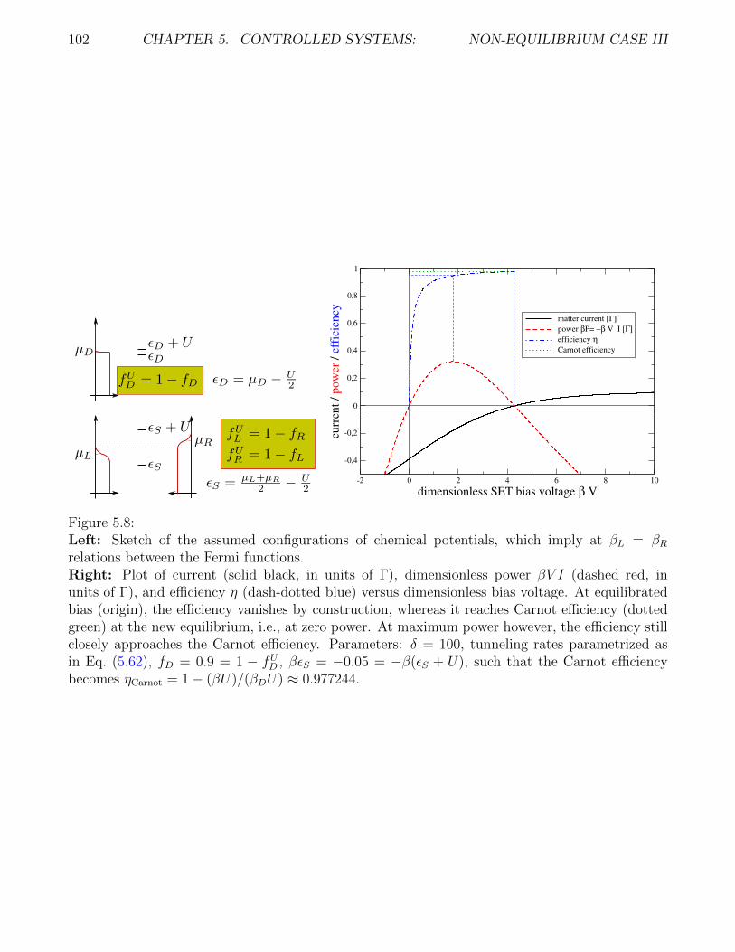
102 CHAPTER 5. CONTROLLED SYSTEMS: NON-EQUILIBRIUM CASE III
-2 0 2 4 6 8 10
dimensionless SET bias voltage β V
-0,4
-0,2
0
0,2
0,4
0,6
0,8
1
curr
ent
/ pow
er /
eff
icie
ncy
matter current [Γ]
power βP= −β V I [Γ]
efficiency η
Carnot efficiency
Figure 5.8:Left: Sketch of the assumed configurations of chemical potentials, which imply at βL = βRrelations between the Fermi functions.Right: Plot of current (solid black, in units of Γ), dimensionless power βV I (dashed red, inunits of Γ), and efficiency η (dash-dotted blue) versus dimensionless bias voltage. At equilibratedbias (origin), the efficiency vanishes by construction, whereas it reaches Carnot efficiency (dottedgreen) at the new equilibrium, i.e., at zero power. At maximum power however, the efficiency stillclosely approaches the Carnot efficiency. Parameters: δ = 100, tunneling rates parametrized asin Eq. (5.62), fD = 0.9 = 1 − fUD , βεS = −0.05 = −β(εS + U), such that the Carnot efficiencybecomes ηCarnot = 1− (βU)/(βDU) ≈ 0.977244.
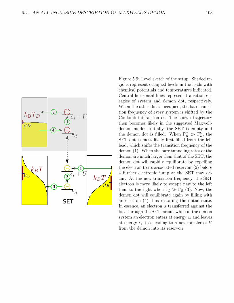
5.4. AN ALL-INCLUSIVE DESCRIPTION OF MAXWELL’S DEMON 103
1
2
3
4
1
2
SET
Figure 5.9: Level sketch of the setup. Shaded re-gions represent occupied levels in the leads withchemical potentials and temperatures indicated.Central horizontal lines represent transition en-ergies of system and demon dot, respectively.When the other dot is occupied, the bare transi-tion frequency of every system is shifted by theCoulomb interaction U . The shown trajectorythen becomes likely in the suggested Maxwell-demon mode: Initially, the SET is empty andthe demon dot is filled. When ΓUR ΓUL , theSET dot is most likely first filled from the leftlead, which shifts the transition frequency of thedemon (1). When the bare tunneling rates of thedemon are much larger than that of the SET, thedemon dot will rapidly equilibrate by expellingthe electron to its associated reservoir (2) beforea further electronic jump at the SET may oc-cur. At the new transition frequency, the SETelectron is more likely to escape first to the leftthan to the right when ΓL ΓR (3). Now, thedemon dot will equilibrate again by filling withan electron (4) thus restoring the initial state.In essence, an electron is transferred against thebias through the SET circuit while in the demonsystem an electron enters at energy εd and leavesat energy εd + U leading to a net transfer of Ufrom the demon into its reservoir.
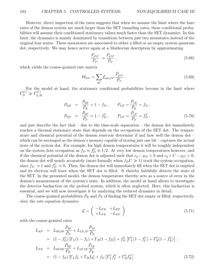
104 CHAPTER 5. CONTROLLED SYSTEMS: NON-EQUILIBRIUM CASE III
However, direct inspection of the rates suggests that when we assume the limit where the barerates of the demon system are much larger than the SET tunneling rates, these conditional proba-bilities will assume their conditioned stationary values much faster than the SET dynamics. In thislimit, the dynamics is mainly dominated by transitions between just two mesostates instead of theoriginal four states. These mesostates are associated to either a filled or an empty system quantumdot, respectively. We may hence arrive again at a Markovian description by approximating
Pρ′σ′
Pσ′→ Pρ′σ′
Pσ′, (5.68)
which yields the coarse-grained rate matrix
Wσσ′ =∑ρρ′
Lρσ,ρ′σ′Pρ′σ′
Pσ′. (5.69)
For the model at hand, the stationary conditional probabilities become in the limit whereΓ
(U)D Γ
(U)L/R
P0|E =P0E
PE= 1− fD , P1|E =
P1E
PE= fD ,
P0|F =P0F
PF= 1− fUD , P1|F =
P1F
PF= fUD , (5.70)
and just describe the fact that – due to the time-scale separation – the demon dot immediatelyreaches a thermal stationary state that depends on the occupation of the SET dot. The temper-ature and chemical potential of the demon reservoir determine if and how well the demon dot –which can be envisaged as the demon’s memory capable of storing just one bit – captures the actualstate of the system dot. For example, for high demon temperatures it will be roughly independenton the system dots occupation as fD ≈ fUD ≈ 1/2. At very low demon temperatures however, andif the chemical potential of the demon dot is adjusted such that εd− µD < 0 and εd +U − µD > 0,the demon dot will nearly accurately (more formally when βDU 1) track the system occupation,since fD → 1 and fUD → 0. Then, the demon dot will immediately fill when the SET dot is emptiedand its electron will leave when the SET dot is filled. It thereby faithfully detects the state ofthe SET. In the presented model, the demon temperature thereby acts as a source of error in thedemon’s measurement of the system’s state. In addition, the model at hand allows to investigatethe detector backaction on the probed system, which is often neglected. Here, this backaction isessential, and we will now investigate it by analyzing the reduced dynamics in detail.
The coarse-grained probabilities PE and PF of finding the SET dot empty or filled, respectively,obey the rate equation dynamics
L =
(−LFE +LEF+LFE −LEF
)(5.71)
with the coarse-grained rates
LEF = L0E,0FP0F
PF+ L1E,1F
P1F
PF= (1− fUD ) [ΓL(1− fL) + ΓR(1− fR)] + fUD
[ΓUL(1− fUL ) + ΓUR(1− fUR )
],
LFE = L0F,0EP0E
PE+ L1F,1E
P1E
PE= (1− fD) [ΓLfL + ΓRfR] + fD
[ΓULf
UL + ΓURf
UR
]. (5.72)
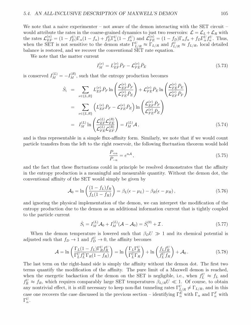
5.4. AN ALL-INCLUSIVE DESCRIPTION OF MAXWELL’S DEMON 105
We note that a naive experimenter – not aware of the demon interacting with the SET circuit –would attribute the rates in the coarse-grained dynamics to just two reservoirs: L = LL +LR withthe rates L(α)
EF = (1− fUD )Γα(1− fα) + fUDΓUα (1− fUα ) and L(α)FE = (1− fD)Γαfα + fDΓUαf
Uα . Thus,
when the SET is not sensitive to the demon state ΓUL/R ≈ ΓL/R and fUL/R ≈ fL/R, local detailedbalance is restored, and we recover the conventional SET rate equation.
We note that the matter current
I(ν)M = L
(ν)EF PF − L
(ν)FEPE (5.73)
is conserved I(L)M = −I(R)
M , such that the entropy production becomes
Si =∑
ν∈L,R
L(ν)EF PF ln
(L(ν)EF PF
L(ν)FEPE
)+ L(ν)
FEPE ln
(L(ν)FEPE
L(ν)EF PF
)
=∑
ν∈L,R
(L
(ν)EF PF − L
(ν)FEPE
)ln
(L(ν)EF PF
L(ν)FEPE
)
= I(L)M ln
(L(L)EFL
(R)FE
L(L)FEL
(R)EF
)= I
(L)M A , (5.74)
and is thus representable in a simple flux-affinity form. Similarly, we note that if we would countparticle transfers from the left to the right reservoir, the following fluctuation theorem would hold
P+n
P−n= enA , (5.75)
and the fact that these fluctuations could in principle be resolved demonstrates that the affinityin the entropy production is a meaningful and measurable quantity. Without the demon dot, theconventional affinity of the SET would simply be given by
A0 = ln
((1− fL)fRfL(1− fR)
)= βL(ε− µL)− βR(ε− µR) , (5.76)
and ignoring the physical implementation of the demon, we can interpret the modification of theentropy production due to the demon as an additional information current that is tightly coupledto the particle current
Si = I(L)M A0 + I
(L)M (A−A0) = S
(0)i + I . (5.77)
When the demon temperature is lowered such that βDU 1 and its chemical potential isadjusted such that fD → 1 and fUD → 0, the affinity becomes
A = ln
(ΓL(1− fL)ΓURf
UR
ΓULfUL ΓR(1− fR)
)= ln
(ΓLΓURΓULΓR
)+ ln
(fLf
UR
fUL fR
)+A0 . (5.78)
The last term on the right-hand side is simply the affinity without the demon dot. The first twoterms quantify the modification of the affinity. The pure limit of a Maxwell demon is reached,when the energetic backaction of the demon on the SET is negligible, i.e., when fUL ≈ fL andfUR ≈ fR, which requires comparably large SET temperatures βL/RU 1. Of course, to obtainany nontrivial effect, it is still necessary to keep non-flat tunneling rates ΓUL/R 6= ΓL/R, and in this
case one recovers the case discussed in the previous section – identifying ΓEα with Γα and ΓFα withΓUα .
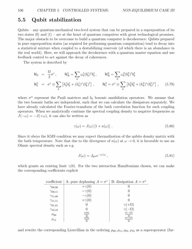
106 CHAPTER 5. CONTROLLED SYSTEMS: NON-EQUILIBRIUM CASE III
5.5 Qubit stabilization
Qubits – any quantum-mechanical two-level system that can be prepared in a superposition of itstwo states |0〉 and |1〉 – are at the heart of quantum computers with great technological promises.The major obstacle to be overcome to build a quantum computer is decoherence: Qubits preparedin pure superposition states (as required for performing quantum computation) tend to decay intoa statistical mixture when coupled to a destabilizing reservoir (of which there is an abundance inthe real world). Here, we will approach the decoherence with a quantum master equation and usefeedback control to act against the decay of coherences.
The system is described by
HS =Ω
2σz , H1
B =∑k
ω1k(b
1k)†b1k , H2
B =∑k
ω2k(b
2k)†b2k
H1I = σz ⊗
∑k
[h1kb
1k + (h1
k)∗(b1
k)†] , H2
I = σx ⊗∑k
[h2kb
2k + (h2
k)∗(b2
k)†] , (5.79)
where σα represent the Pauli matrices and bk bosonic annihilation operators. We assume thatthe two bosonic baths are independent, such that we can calculate the dissipators separately. Wehave already calculated the Fourier-transform of the bath correlation function for such couplingoperators. When we analytically continue the spectral coupling density to negative frequencies asJ(−ω) = −J(+ω), it can also be written as
γ(ω) = J(ω) [1 + n(ω)] . (5.80)
Since it obeys the KMS condition we may expect thermalization of the qubits density matrix withthe bath temperature. Note that due to the divergence of n(ω) at ω → 0, it is favorable to use anOhmic spectral density such as e.g.
J(ω) = J0ωe−ω/ωc , (5.81)
which grants an existing limit γ(0). For the two interaction Hamiltonians chosen, we can makethe corresponding coefficients explicit
coefficient A: pure dephasing A = σz B: dissipation A = σx
γ00,00 +γ(0) 0γ00,11 −γ(0) 0γ11,00 −γ(0) 0γ11,11 +γ(0) 0γ01,01 0 γ(+Ω)γ10,10 0 γ(−Ω)
σ00σ(0)2i
σ(−Ω)2i
σ11σ(0)2i
σ(+Ω)2i
and rewrite the corresponding Liouvillian in the ordering ρ00, ρ11, ρ01, ρ10 as a superoperator (fur-
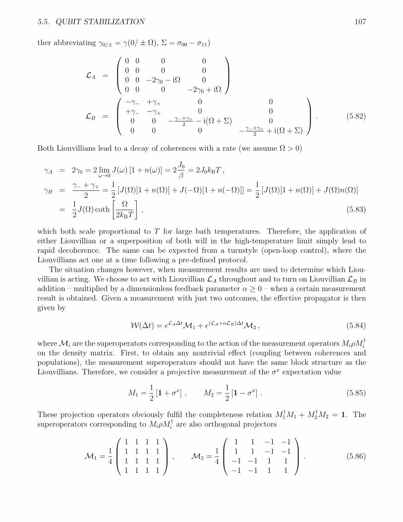
5.5. QUBIT STABILIZATION 107
ther abbreviating γ0/± = γ(0/± Ω), Σ = σ00 − σ11)
LA =
0 0 0 00 0 0 00 0 −2γ0 − iΩ 00 0 0 −2γ0 + iΩ
LB =
−γ− +γ+ 0 0+γ− −γ+ 0 0
0 0 −γ−+γ+
2− i(Ω + Σ) 0
0 0 0 −γ−+γ+
2+ i(Ω + Σ)
. (5.82)
Both Liouvillians lead to a decay of coherences with a rate (we assume Ω > 0)
γA = 2γ0 = 2 limω→0
J(ω) [1 + n(ω)] = 2J0
β= 2J0kBT ,
γB =γ− + γ+
2=
1
2[J(Ω)[1 + n(Ω)] + J(−Ω)[1 + n(−Ω)]] =
1
2[J(Ω)[1 + n(Ω)] + J(Ω)n(Ω)]
=1
2J(Ω) coth
[Ω
2kBT
], (5.83)
which both scale proportional to T for large bath temperatures. Therefore, the application ofeither Liouvillian or a superposition of both will in the high-temperature limit simply lead torapid decoherence. The same can be expected from a turnstyle (open-loop control), where theLiouvillians act one at a time following a pre-defined protocol.
The situation changes however, when measurement results are used to determine which Liou-villian is acting. We choose to act with Liouvillian LA throughout and to turn on Liouvillian LB inaddition – multiplied by a dimensionless feedback parameter α ≥ 0 – when a certain measurementresult is obtained. Given a measurement with just two outcomes, the effective propagator is thengiven by
W(∆t) = eLA∆tM1 + e(LA+αLB)∆tM2 , (5.84)
whereMi are the superoperators corresponding to the action of the measurement operators MiρM†i
on the density matrix. First, to obtain any nontrivial effect (coupling between coherences andpopulations), the measurement superoperators should not have the same block structure as theLiouvillians. Therefore, we consider a projective measurement of the σx expectation value
M1 =1
2[1 + σx] , M2 =
1
2[1− σx] . (5.85)
These projection operators obviously fulfil the completeness relation M †1M1 + M †
2M2 = 1. Thesuperoperators corresponding to MiρM
†i are also orthogonal projectors
M1 =1
4
1 1 1 11 1 1 11 1 1 11 1 1 1
, M2 =1
4
1 1 −1 −11 1 −1 −1−1 −1 1 1−1 −1 1 1
. (5.86)
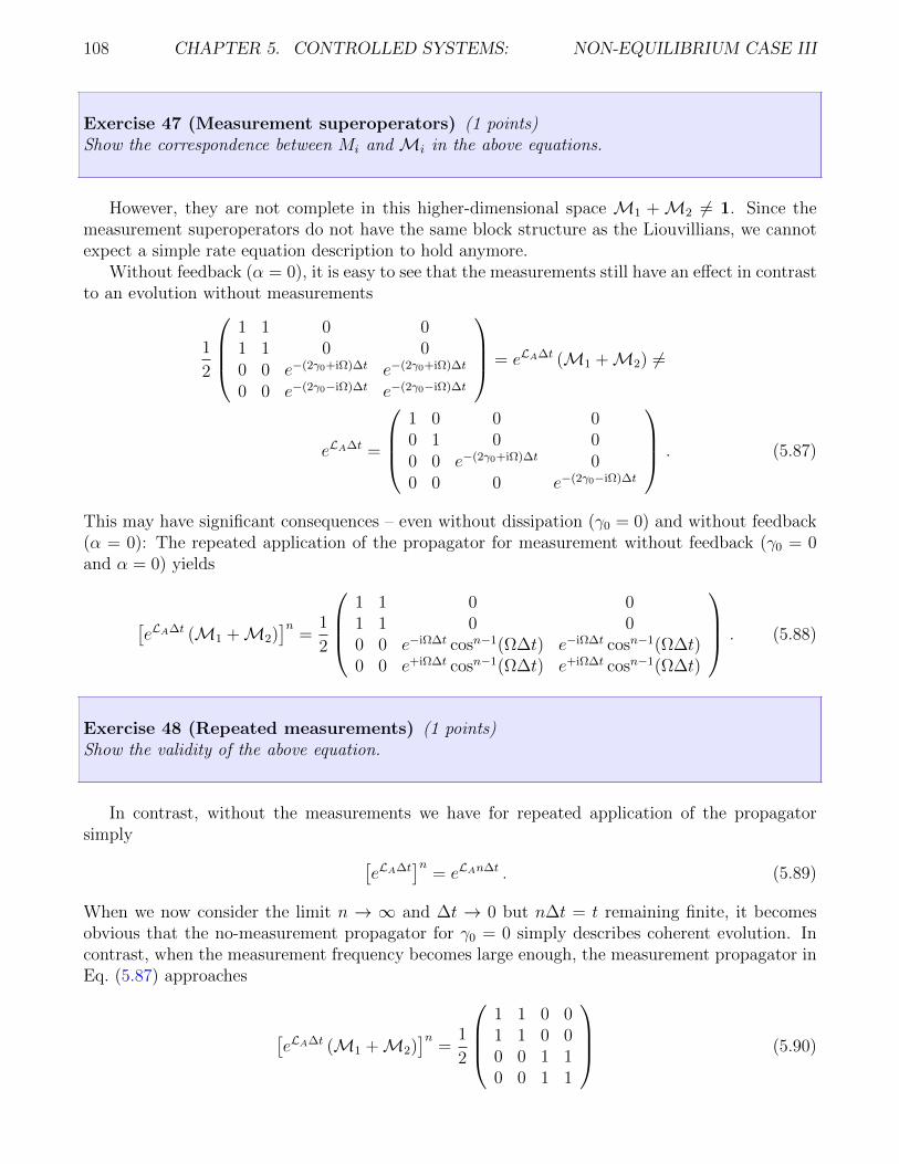
108 CHAPTER 5. CONTROLLED SYSTEMS: NON-EQUILIBRIUM CASE III
Exercise 47 (Measurement superoperators) (1 points)Show the correspondence between Mi and Mi in the above equations.
However, they are not complete in this higher-dimensional space M1 +M2 6= 1. Since themeasurement superoperators do not have the same block structure as the Liouvillians, we cannotexpect a simple rate equation description to hold anymore.
Without feedback (α = 0), it is easy to see that the measurements still have an effect in contrastto an evolution without measurements
1
2
1 1 0 01 1 0 00 0 e−(2γ0+iΩ)∆t e−(2γ0+iΩ)∆t
0 0 e−(2γ0−iΩ)∆t e−(2γ0−iΩ)∆t
= eLA∆t (M1 +M2) 6=
eLA∆t =
1 0 0 00 1 0 00 0 e−(2γ0+iΩ)∆t 00 0 0 e−(2γ0−iΩ)∆t
. (5.87)
This may have significant consequences – even without dissipation (γ0 = 0) and without feedback(α = 0): The repeated application of the propagator for measurement without feedback (γ0 = 0and α = 0) yields
[eLA∆t (M1 +M2)
]n=
1
2
1 1 0 01 1 0 00 0 e−iΩ∆t cosn−1(Ω∆t) e−iΩ∆t cosn−1(Ω∆t)0 0 e+iΩ∆t cosn−1(Ω∆t) e+iΩ∆t cosn−1(Ω∆t)
. (5.88)
Exercise 48 (Repeated measurements) (1 points)Show the validity of the above equation.
In contrast, without the measurements we have for repeated application of the propagatorsimply [
eLA∆t]n
= eLAn∆t . (5.89)
When we now consider the limit n → ∞ and ∆t → 0 but n∆t = t remaining finite, it becomesobvious that the no-measurement propagator for γ0 = 0 simply describes coherent evolution. Incontrast, when the measurement frequency becomes large enough, the measurement propagator inEq. (5.87) approaches
[eLA∆t (M1 +M2)
]n=
1
2
1 1 0 01 1 0 00 0 1 10 0 1 1
(5.90)
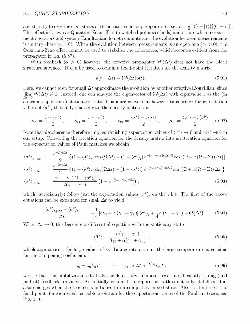
5.5. QUBIT STABILIZATION 109
and thereby freezes the eigenstates of the measurement superoperators, e.g. ρ = 12
[|0〉+ |1〉] [〈0|+ 〈1|].This effect is known as Quantum-Zeno effect (a watched pot never boils) and occurs when measure-ment operators and system Hamiltonian do not commute and the evolution between measurementsis unitary (here γ0 = 0). When the evolution between measurements is an open one (γ0 > 0), theQuantum-Zeno effect cannot be used to stabilize the coherences, which becomes evident from thepropagator in Eq. (5.87).
With feedback (α > 0) however, the effective propagator W(∆t) does not have the Blockstructure anymore. It can be used to obtain a fixed-point iteration for the density matrix
ρ(t+ ∆t) =W(∆t)ρ(t) . (5.91)
Here, we cannot even for small ∆t approximate the evolution by another effective Liouvillian, sincelim
∆t→0W(∆t) 6= 1. Instead, one can analyze the eigenvector of W(∆t) with eigenvalue 1 as the (in
a stroboscopic sense) stationary state. It is more convenient however to consider the expectationvalues of 〈σi〉t that fully characterize the density matrix via
ρ00 =1 + 〈σz〉
2, ρ11 =
1− 〈σz〉2
, ρ01 =〈σx〉 − i 〈σy〉
2, ρ10 =
〈σx〉+ i 〈σy〉2
. (5.92)
Note that decoherence therefore implies vanishing expectation values of 〈σx〉 → 0 and 〈σy〉 → 0 inour setup. Converting the iteration equation for the density matrix into an iteration equation forthe expectation values of Pauli matrices we obtain
〈σx〉t+∆t =e−2γ0∆t
2
(1 + 〈σx〉t) cos (Ω∆t)− (1− 〈σx〉t) e
−(γ−+γ+)α∆t/2 cos [(Ω + α(Ω + Σ)) ∆t]
〈σy〉t+∆t =e−2γ0∆t
2
(1 + 〈σx〉t) sin (Ω∆t)− (1− 〈σx〉t) e
−(γ−+γ+)α∆t/2 sin [(Ω + α(Ω + Σ)) ∆t]
〈σz〉t+∆t =(γ+ − γ−) (1− 〈σx〉t)
2(γ− + γ+)
(1− e−(γ−+γ+)α∆t
), (5.93)
which (surprisingly) follow just the expectation values 〈σx〉t on the r.h.s. The first of the aboveequations can be expanded for small ∆t to yield
〈σx〉t+∆t − 〈σx〉t∆t
= −1
4[8γ0 + α (γ− + γ+)] 〈σx〉t +
1
4α (γ− + γ+) +O∆t . (5.94)
When ∆t→ 0, this becomes a differential equation with the stationary state
〈σx〉 =α(γ− + γ+)
8γ0 + α(γ− + γ+), (5.95)
which approaches 1 for large values of α. Taking into account the large-temperature expansionsfor the dampening coefficients
γ0 = J0kBT , γ− + γ+ ≈ 2J0e−Ω/ωckBT , (5.96)
we see that this stabilization effect also holds at large temperatures – a sufficiently strong (andperfect) feedback provided. An initially coherent superposition is thus not only stabilized, butalso emerges when the scheme is initialized in a completely mixed state. Also for finite ∆t, thefixed-point iteration yields sensible evolution for the expectation values of the Pauli matrices, seeFig. 5.10.
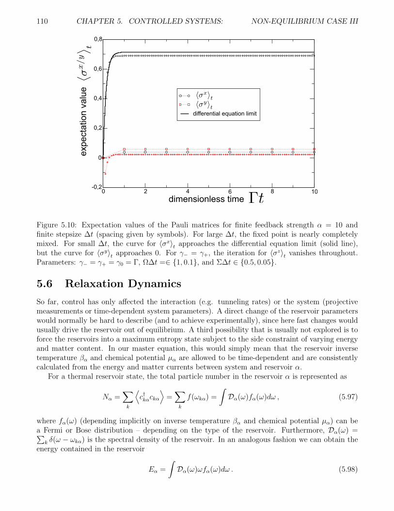
110 CHAPTER 5. CONTROLLED SYSTEMS: NON-EQUILIBRIUM CASE III
0 2 4 6 8 10
dimensionless time
-0,2
0
0,2
0,4
0,6
0,8
expe
cta
tion
va
lue
differential equation limit
Figure 5.10: Expectation values of the Pauli matrices for finite feedback strength α = 10 andfinite stepsize ∆t (spacing given by symbols). For large ∆t, the fixed point is nearly completelymixed. For small ∆t, the curve for 〈σx〉t approaches the differential equation limit (solid line),but the curve for 〈σy〉t approaches 0. For γ− = γ+, the iteration for 〈σz〉t vanishes throughout.Parameters: γ− = γ+ = γ0 = Γ, Ω∆t =∈ 1, 0.1, and Σ∆t ∈ 0.5, 0.05.
5.6 Relaxation Dynamics
So far, control has only affected the interaction (e.g. tunneling rates) or the system (projectivemeasurements or time-dependent system parameters). A direct change of the reservoir parameterswould normally be hard to describe (and to achieve experimentally), since here fast changes wouldusually drive the reservoir out of equilibrium. A third possibility that is usually not explored is toforce the reservoirs into a maximum entropy state subject to the side constraint of varying energyand matter content. In our master equation, this would simply mean that the reservoir inversetemperature βα and chemical potential µα are allowed to be time-dependent and are consistentlycalculated from the energy and matter currents between system and reservoir α.
For a thermal reservoir state, the total particle number in the reservoir α is represented as
Nα =∑k
⟨c†kαckα
⟩=∑k
f(ωkα) =
∫Dα(ω)fα(ω)dω , (5.97)
where fα(ω) (depending implicitly on inverse temperature βα and chemical potential µα) can bea Fermi or Bose distribution – depending on the type of the reservoir. Furthermore, Dα(ω) =∑
k δ(ω − ωkα) is the spectral density of the reservoir. In an analogous fashion we can obtain theenergy contained in the reservoir
Eα =
∫Dα(ω)ωfα(ω)dω . (5.98)
5.6. RELAXATION DYNAMICS 111
Total conservation of charge and energy implies that given charge and energy currents into thereservoir
Nα = −I(α)M =
∂Nα
∂µαµα +
∂Nα
∂βα
dβαdTα
Tα ,
Eα = −I(α)E =
∂Eα∂µα
µα +∂Eα∂βα
dβαdTα
Tα (5.99)
one can calculate the change of reservoir charge and energy. Here however, we will be interested inthe change of reservoir temperature and chemical potential, for which we can obtain a differentialequation by solving the above equations for µα and Tα. For example, in case of fermions, we canfirst solve for
∂Nα
∂µα=
∫Dα(ω)fα(ω)[1− fα(ω)]dωβα = I1βα ,
∂Nα
∂βα= −
∫Dα(ω)fα(ω)[1− fα(ω)](ω − µα)dω = −I2 ,
∂Eα∂µα
=
∫Dα(ω)ωfα(ω)[1− fα(ω)]dωβα = (I2 + µαI1)βα ,
∂Eα∂βα
= −∫Dα(ω)ωfα(ω)[1− fα(ω)](ω − µα)dω = −I3 − µαI2 . (5.100)
Here, we have defined three integrals
I1 =
∫Dα(ω)f(ω)[1− fα(ω)]dω , I2 =
∫Dα(ω)(ω − µα)fα(ω)[1− fα(ω)]dω ,
I3 =
∫Dα(ω)(ω − µα)2fα(ω)[1− fα(ω)]dω , (5.101)
which in the wide-band limit Dα(ω) = Dα can be solved exactly
I1 =Dα
βα= DαTα , I2 = 0 , I3 =
π2
3
Dα
β3α
=π2
3DαT
3α . (5.102)
Exercise 49 (Fermi integrals) Show validity of Eq. (5.102). You might want to use that∫ ∞0
ln2(x)
(x+ 1)2=π2
3. (5.103)
From these, we obtain a simple relation between currents and thermodynamic parameters(−I(α)
M
−I(α)E
)= Dα
(1 0
µ π2
3Tα
)(µαTα
). (5.104)
We can directly invert the matrix containing the heat and charge capacities to solve for the firstderivatives (
µαTα
)=
1
Dα
(1 0
− 3π2
µαTα
3π2
1Tα
)(−I(α)
M
−I(α)E
). (5.105)
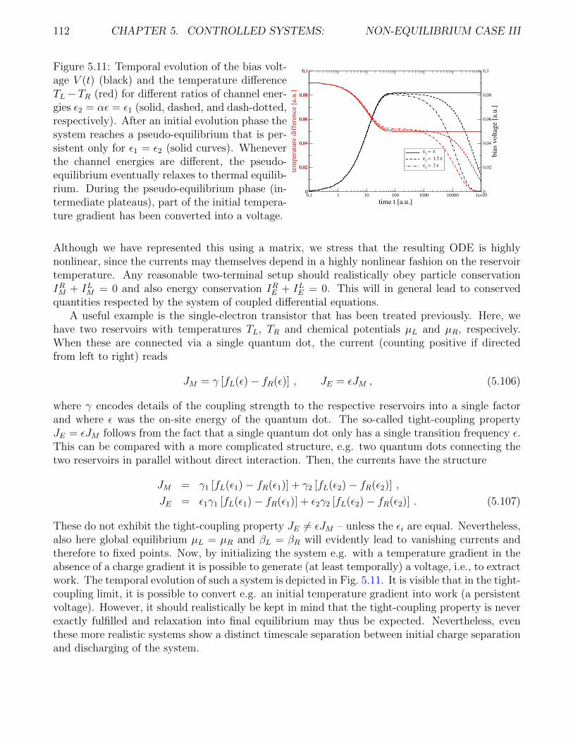
112 CHAPTER 5. CONTROLLED SYSTEMS: NON-EQUILIBRIUM CASE III
Figure 5.11: Temporal evolution of the bias volt-age V (t) (black) and the temperature differenceTL−TR (red) for different ratios of channel ener-gies ε2 = αε = ε1 (solid, dashed, and dash-dotted,respectively). After an initial evolution phase thesystem reaches a pseudo-equilibrium that is per-sistent only for ε1 = ε2 (solid curves). Wheneverthe channel energies are different, the pseudo-equilibrium eventually relaxes to thermal equilib-rium. During the pseudo-equilibrium phase (in-termediate plateaus), part of the initial tempera-ture gradient has been converted into a voltage.
0,1 1 10 100 1000 10000 1e+05
time t [a.u.]
0 0
0,02 0,02
0,04 0,04
0,06 0,06
0,08 0,08
0,1 0,1
tem
per
ature
dif
fere
nce
[a.
u.]
0
0,02
0,04
0,06
0,08
0,1
bia
s volt
age
[a.u
.]
ε2 = ε
ε2 = 1.5 ε
ε2 = 2 ε
Although we have represented this using a matrix, we stress that the resulting ODE is highlynonlinear, since the currents may themselves depend in a highly nonlinear fashion on the reservoirtemperature. Any reasonable two-terminal setup should realistically obey particle conservationIRM + ILM = 0 and also energy conservation IRE + ILE = 0. This will in general lead to conservedquantities respected by the system of coupled differential equations.
A useful example is the single-electron transistor that has been treated previously. Here, wehave two reservoirs with temperatures TL, TR and chemical potentials µL and µR, respecively.When these are connected via a single quantum dot, the current (counting positive if directedfrom left to right) reads
JM = γ [fL(ε)− fR(ε)] , JE = εJM , (5.106)
where γ encodes details of the coupling strength to the respective reservoirs into a single factorand where ε was the on-site energy of the quantum dot. The so-called tight-coupling propertyJE = εJM follows from the fact that a single quantum dot only has a single transition frequency ε.This can be compared with a more complicated structure, e.g. two quantum dots connecting thetwo reservoirs in parallel without direct interaction. Then, the currents have the structure
JM = γ1 [fL(ε1)− fR(ε1)] + γ2 [fL(ε2)− fR(ε2)] ,
JE = ε1γ1 [fL(ε1)− fR(ε1)] + ε2γ2 [fL(ε2)− fR(ε2)] . (5.107)
These do not exhibit the tight-coupling property JE 6= εJM – unless the εi are equal. Nevertheless,also here global equilibrium µL = µR and βL = βR will evidently lead to vanishing currents andtherefore to fixed points. Now, by initializing the system e.g. with a temperature gradient in theabsence of a charge gradient it is possible to generate (at least temporally) a voltage, i.e., to extractwork. The temporal evolution of such a system is depicted in Fig. 5.11. It is visible that in the tight-coupling limit, it is possible to convert e.g. an initial temperature gradient into work (a persistentvoltage). However, it should realistically be kept in mind that the tight-coupling property is neverexactly fulfilled and relaxation into final equilibrium may thus be expected. Nevertheless, eventhese more realistic systems show a distinct timescale separation between initial charge separationand discharging of the system.