Embed Size (px)
Citation preview


Non-Equilibrium Thermodynamicsof Heterogeneous Systems
SERIES ON ADVANCES IN STATISTICAL MECHANICS*
Editor -in-Chief: M. Rasetti (Politecnico di Torino, Italy)
Published
Vol. 6: New Problems, Methods and Techniques in Quantum Field Theoryand Statistical Mechanicsedited by M. Rasetti
Vol. 7: The Hubbard Model – Recent Resultsedited by M. Rasetti
Vol. 8: Statistical Thermodynamics and Stochastic Theory of NonlinearSystems Far From Equilibriumby W. Ebeling & L. Schimansky-Geier
Vol. 9: Disorder and Competition in Soluble Lattice Modelsby W. F. Wreszinski & S. R. A. Salinas
Vol. 10: An Introduction to Stochastic Processes and NonequilibriumStatistical Physicsby H. S. Wio
Vol. 12: Quantum Many-Body Systems in One Dimensionby Zachary N. C. Ha
Vol. 13: Exactly Soluble Models in Statistical Mechanics: Historical Perspectivesand Current Statusedited by C. King & F. Y. Wu
Vol. 14: Statistical Physics on the Eve of the 21st Century: In Honour ofJ. B. McGuire on the Occasion of his 65th Birthdayedited by M. T. Batchelor & L. T. Wille
Vol. 15: Lattice Statistics and Mathematical Physics: Festschrift Dedicated toProfessor Fa-Yueh Wu on the Occasion of his 70th Birthdayedited by J. H. H. Perk & M.-L. Ge
Vol. 16: Non-Equilibrium Thermodynamics of Heterogeneous Systemsby S. Kjelstrup & D. Bedeaux
*For the complete list of titles in this series, please go to
http://www.worldscibooks.com/series/sasm_series
Alvin - Non-Equilibrium.pmd 12/28/2007, 10:13 AM2

Series on Advances in Statistical Mechanics -- Volume 16
Non-Equilibrium Thermodynamicsof Heterogeneous Systems
SIGNE KJELSTRUP DICK BEDEAUX
Norwegian University of Science and Technology
World ScientificNEW JERSEY . LONDON . SINGAPORE . BEIJING . SHANGHAI . HOND KONG . TAIPEI . CHENNAI

British Library Cataloguing-in-Publication DataA catalogue record for this book is available from the British Library.
For photocopying of material in this volume, please pay a copying fee through the CopyrightClearance Center, Inc., 222 Rosewood Drive, Danvers, MA 01923, USA. In this case permission tophotocopy is not required from the publisher.
ISBN-13 978-981-277-913-7ISBN-10 981-277-913-2
All rights reserved. This book, or parts thereof, may not be reproduced in any form or by any means,electronic or mechanical, including photocopying, recording or any information storage and retrievalsystem now known or to be invented, without written permission from the Publisher.
Copyright © 2008 by World Scientific Publishing Co. Pte. Ltd.
Published by
World Scientific Publishing Co. Pte. Ltd.
5 Toh Tuck Link, Singapore 596224
USA office: 27 Warren Street, Suite 401-402, Hackensack, NJ 07601
UK office: 57 Shelton Street, Covent Garden, London WC2H 9HE
Printed in Singapore.
Series on Advances in Statistical Mechanics – Vol. 16NON-EQUILIBRIUM THERMODYNAMICS OF HETEROGENEOUS SYSTEMS
Alvin - Non-Equilibrium.pmd 12/28/2007, 10:13 AM1

We dedicate this book to our teacher and friend Peter Mazur
v

This page intentionally left blankThis page intentionally left blank

Preface
What the book is about
This book describes transport through complex, heterogeneous media.There are large coupling effects between transports of heat, mass, chargeand chemical reactions in such media, and it is important to know howone should properly integrate across heterogeneous systems where differentphases are in contact. Transports perpendicular to planar interfaces aretreated.
How we were inspired to write it
Waldmann [1] was the first to point out that an analysis of boundary con-ditions should be incorporated in the framework of non-equilibrium ther-modynamics. He did not include excess densities to describe the propertiesof the surface, however. In the 1970s and 1980s Bedeaux, Albano andMazur [2–4] extended his work and laid the theoretical foundation for thedescription of non-equilibrium processes, including a full description of thethermodynamic properties of the surface. The work of Bedeaux, Albanoand Mazur addressed not only transports into and through a surface, butalso transports along surfaces as well as the motion of the surface itself.Their methods were inspired by concurrent work on the optical propertiesof surfaces by Bedeaux and Vlieger [5, 6], using generalized functions forthe description of surface properties. The present work takes advantage ofthese methodologies.
Who it is meant for
The purpose of this book is to encourage the use of non-equilibriumthermodynamics to describe transport in complex, heterogeneous media.The book is written for a graduate level course for physicists, physicalchemists, chemical or mechanical engineers. The book requires knowledgeof basic thermodynamics corresponding to that given by Atkins, Physical
vii

viii Preface
Chemistry (Oxford University Press), or Moran and Shapiro, Fundamentalsof Engineering Thermodynamics (John Wiley & Sons).
Acknowledgments
A course on non-equilibrium thermodynamics has been taught at the Nor-wegian University of Science and Technology for many years. We aregrateful to the graduate students who worked with us on related subjectsand commented on preliminary versions of the text. In alphabetical order,we would like to mention Odne Stokke Burheim, Belinda Flem, AndreasGrimstvedt, Kirill Glavatskiy, Ellen Marie Hansen, Torleif Holt, IsabellaInzoli, Eivind Johannessen, Einar Eng Johnsen, Gelein de Koeijer, LarsNummedal, Anne-Kristine Meland, Steffen Møller-Holst, Magnar Ottøy,Audun Røsjorde, Erik Sauar, Kristin Syverud, Preben Joakim Svela Vie,Jing Xu and Anita Zvolinschi. Discussions and collaborations with col-leagues Bjørn Hafskjold, Jean-Marc Simon, Fernando Bresme and EdgarBlokhuis were appreciated.
During our peaceful and inspiring stay in Kyoto University in 2000,a large step forward was made. We are grateful to our host Prof. Ya-suhiko Ito, and to coworkers, Profs. Yoichi Tomii, Yasuhiro Fukunaka, Drs.Toshiyuki Nohira and Koji Amezawa. The next large step was made inbeautiful Barcelona in 2004, with our considerate host, Prof. Miguel Rubiof University of Barcelona.
We thank the Research Council of Norway for financial support overmany years. Marian Palcut contributed the cover image, while TharaldTharaldsen, Jaques van der Ploeg and Michel Uiterwijk contributed manyfigures.
Signe Kjelstrup∗ and Dick Bedeaux March 2008
Address for correspondence:
Department of Chemistry,Norwegian University of Science and Technology,NO-7491 Trondheim, Norway
∗The author changed her name from Ratkje to Kjelstrup in 1996.

Contents
Preface . . . . . . . . . . . . . . . . . . . . . . . . . . . . . . . . vii
1 Scope 1
1.1 What is non-equilibrium thermodynamics? . . . . . . . . . 11.2 Non-equilibrium thermodynamics in the context of
other theories . . . . . . . . . . . . . . . . . . . . . . . . . 41.3 The purpose of this book . . . . . . . . . . . . . . . . . . . 4
2 Why Non-Equilibrium Thermodynamics? 7
2.1 Simple flux equations . . . . . . . . . . . . . . . . . . . . . 82.2 Flux equations with coupling terms . . . . . . . . . . . . . 92.3 Experimental designs and controls . . . . . . . . . . . . . . 112.4 Entropy production, work and lost work . . . . . . . . . . 122.5 Consistent thermodynamic models . . . . . . . . . . . . . . 14
3 Thermodynamic Relations for Heterogeneous Systems 17
3.1 Two homogeneous phases separated by a surface in globalequilibrium . . . . . . . . . . . . . . . . . . . . . . . . . . . 18
3.2 The contact line in global equilibrium . . . . . . . . . . . . 223.3 Defining thermodynamic variables for the surface . . . . . 233.4 Local thermodynamic identities . . . . . . . . . . . . . . . 293.5 Defining local equilibrium . . . . . . . . . . . . . . . . . . 323.A Appendix: Partial molar properties . . . . . . . . . . . . . 35
3.A.1 Homogeneous phases . . . . . . . . . . . . . . . . . 363.A.2 The surface . . . . . . . . . . . . . . . . . . . . . . 383.A.3 The standard state . . . . . . . . . . . . . . . . . . 40
Part A: General Theory 45
4 The Entropy Production for a Homogeneous Phase 47
4.1 Balance equations . . . . . . . . . . . . . . . . . . . . . . . 494.2 The entropy production . . . . . . . . . . . . . . . . . . . . 51
ix

x Contents
4.2.1 Why one should not use the dissipation function . 564.2.2 States with minimum entropy production . . . . . 57
4.3 Examples . . . . . . . . . . . . . . . . . . . . . . . . . . . . 584.4 Frames of reference for fluxes in homogeneous systems . . 64
4.4.1 Definitions of frames of reference . . . . . . . . . . 644.4.2 Transformations between the frames of reference . 66
4.A Appendix: The first law and the heat flux . . . . . . . . . 67
5 The Excess Entropy Production for the Surface 73
5.1 The discrete nature of the surface . . . . . . . . . . . . . . 745.2 The behavior of the electric fields and potential through the
surface . . . . . . . . . . . . . . . . . . . . . . . . . . . . . 755.3 Balance equations . . . . . . . . . . . . . . . . . . . . . . . 775.4 The excess entropy production . . . . . . . . . . . . . . . . 79
5.4.1 Reversible processes at the interface and the Nernstequation . . . . . . . . . . . . . . . . . . . . . . . 84
5.4.2 The surface potential jump at the hydrogenelectrode . . . . . . . . . . . . . . . . . . . . . . . 86
5.5 Examples . . . . . . . . . . . . . . . . . . . . . . . . . . . . 87
6 The Excess Entropy Production for a Three Phase
Contact Line 91
6.1 The discrete nature of the contact line . . . . . . . . . . . 926.2 Balance equations . . . . . . . . . . . . . . . . . . . . . . . 946.3 The excess entropy production . . . . . . . . . . . . . . . . 956.4 Stationary states . . . . . . . . . . . . . . . . . . . . . . . 966.5 Concluding comment . . . . . . . . . . . . . . . . . . . . . 97
7 Flux Equations and Onsager Relations 99
7.1 Flux-force relations . . . . . . . . . . . . . . . . . . . . . . 997.2 Onsager’s reciprocal relations . . . . . . . . . . . . . . . . 1007.3 Relaxation to equilibrium. Consequences of violating
Onsager relations . . . . . . . . . . . . . . . . . . . . . . . 1047.4 Force-flux relations . . . . . . . . . . . . . . . . . . . . . . 1057.5 Coefficient bounds . . . . . . . . . . . . . . . . . . . . . . 1067.6 The Curie principle applied to surfaces and contact lines . 108
8 Transport of Heat and Mass 111
8.1 The homogeneous phases . . . . . . . . . . . . . . . . . . . 1128.2 Coefficient values for homogeneous phases . . . . . . . . . 1148.3 The surface . . . . . . . . . . . . . . . . . . . . . . . . . . 117
8.3.1 Heats of transfer for the surface . . . . . . . . . . 119

Contents xi
8.4 Solution for the heterogeneous system . . . . . . . . . . . . 1228.5 Scaling relations between surface and bulk resistivities . . 125
9 Transport of Heat and Charge 127
9.1 The homogeneous phases . . . . . . . . . . . . . . . . . . . 1289.2 The surface . . . . . . . . . . . . . . . . . . . . . . . . . . 1309.3 Thermoelectric coolers . . . . . . . . . . . . . . . . . . . . 1329.4 Thermoelectric generators . . . . . . . . . . . . . . . . . . 1339.5 Solution for the heterogeneous system . . . . . . . . . . . . 135
10 Transport of Mass and Charge 139
10.1 The electrolyte . . . . . . . . . . . . . . . . . . . . . . . . . 14010.2 The electrode surfaces . . . . . . . . . . . . . . . . . . . . 14310.3 Solution for the heterogeneous system . . . . . . . . . . . . 14610.4 A salt power plant . . . . . . . . . . . . . . . . . . . . . . 14710.5 Electric power from volume flow . . . . . . . . . . . . . . . 14810.6 Ionic mobility model for the electrolyte . . . . . . . . . . . 15010.7 Ionic and electronic model for the surface . . . . . . . . . . 154
Part B: Applications 155
11 Evaporation and Condensation 157
11.1 Evaporation and condensation in a pure fluid . . . . . . . 15811.1.1 The entropy production and the flux equations . . 15811.1.2 Interface resistivities from kinetic theory . . . . . 165
11.2 The sign of the heats of transfer of the surface . . . . . . . 16711.3 Coefficients from molecular dynamics simulations . . . . . 16911.4 Evaporation and condensation in a two-component fluid . 176
11.4.1 The entropy production and the flux equations . . 17611.4.2 Interface resistivities from kinetic theory . . . . . 179
12 Multi-Component Heat and Mass Diffusion 183
12.1 The homogeneous phases . . . . . . . . . . . . . . . . . . . 18412.2 The Maxwell–Stefan equations for multi-component
diffusion . . . . . . . . . . . . . . . . . . . . . . . . . . . . 18612.3 The Maxwell–Stefan equations for the surface . . . . . . . 18812.4 Multi-component diffusion . . . . . . . . . . . . . . . . . . 192
12.4.1 Prigogine’s theorem . . . . . . . . . . . . . . . . . 19212.4.2 Diffusion in the solvent frame of reference . . . . . 19312.4.3 Other frames of reference . . . . . . . . . . . . . . 19512.4.4 An example: Kinetic demixing of oxides . . . . . . 200

xii Contents
12.5 A relation between the heats of transfer andthe enthalpy . . . . . . . . . . . . . . . . . . . . . . . . . . 202
13 A Nonisothermal Concentration Cell 205
13.1 The homogeneous phases . . . . . . . . . . . . . . . . . . . 20713.1.1 Entropy production and flux equations for
the anode . . . . . . . . . . . . . . . . . . . . . . . 20713.1.2 Position dependent transport coefficients . . . . . 21013.1.3 The profiles of the homogeneous anode . . . . . . 21113.1.4 Contributions from the cathode . . . . . . . . . . 21213.1.5 The electrolyte contribution . . . . . . . . . . . . 213
13.2 Surface contributions . . . . . . . . . . . . . . . . . . . . . 21413.2.1 The anode surface . . . . . . . . . . . . . . . . . . 21413.2.2 The cathode surface . . . . . . . . . . . . . . . . 217
13.3 The thermoelectric potential . . . . . . . . . . . . . . . . 218
14 The Transported Entropy 221
14.1 The Seebeck coefficient of cell a . . . . . . . . . . . . . . . 22214.2 The transported entropy of Pb2+ in cell a . . . . . . . . . 22614.3 The transported entropy of the cation in cell b . . . . . . . 22714.4 The transported entropy of the ions cell c . . . . . . . . . 22814.5 Transformation properties . . . . . . . . . . . . . . . . . . 23014.6 Concluding comments . . . . . . . . . . . . . . . . . . . . . 232
15 Adiabatic Electrode Reactions 235
15.1 The homogeneous phases . . . . . . . . . . . . . . . . . . . 23615.1.1 The silver phases . . . . . . . . . . . . . . . . . . . 23615.1.2 The silver chloride phases . . . . . . . . . . . . . . 23615.1.3 The electrolyte . . . . . . . . . . . . . . . . . . . . 237
15.2 The interfaces . . . . . . . . . . . . . . . . . . . . . . . . . 23715.2.1 The silver-silver chloride interfaces . . . . . . . . . 23715.2.2 The silver chloride-electrolyte interfaces . . . . . . 239
15.3 Temperature and electric potential profiles . . . . . . . . . 240
16 The Liquid Junction Potential 249
16.1 The flux equations for the electrolyte . . . . . . . . . . . . 25016.2 The liquid junction potential . . . . . . . . . . . . . . . . . 25316.3 Liquid junction potential calculations compared . . . . . . 25516.4 Concluding comments . . . . . . . . . . . . . . . . . . . . . 258

Contents xiii
17 The Formation Cell 261
17.1 The isothermal cell . . . . . . . . . . . . . . . . . . . . . . 26317.1.1 The electromotive force . . . . . . . . . . . . . . . 26317.1.2 The transference coefficient of the salt in
the electrolyte . . . . . . . . . . . . . . . . . . . . 26317.1.3 An electrolyte with a salt concentration gradient . 26517.1.4 The Planck potential derived from ionic fluxes
and forces . . . . . . . . . . . . . . . . . . . . . . . 26717.2 A non-isothermal cell with a non-uniform electrolyte . . . 268
17.2.1 The homogeneous anode phase . . . . . . . . . . . 26917.2.2 The electrolyte . . . . . . . . . . . . . . . . . . . . 27017.2.3 The surface of the anode . . . . . . . . . . . . . . 27217.2.4 The homogeneous phases and the surface of
the cathode . . . . . . . . . . . . . . . . . . . . . . 27317.2.5 The cell potential . . . . . . . . . . . . . . . . . . 275
17.3 Concluding comments . . . . . . . . . . . . . . . . . . . . . 275
18 Power from Regular and Thermal Osmosis 277
18.1 The potential work of a salt power plant . . . . . . . . . . 27718.2 The membrane as a barrier to transport of heat
and mass . . . . . . . . . . . . . . . . . . . . . . . . . . . . 27918.3 Membrane transport of heat and mass . . . . . . . . . . . 28118.4 Osmosis . . . . . . . . . . . . . . . . . . . . . . . . . . . . 28318.5 Thermal osmosis . . . . . . . . . . . . . . . . . . . . . . . . 285
19 Modeling the Polymer Electrolyte Fuel Cell 289
19.1 The potential work of a fuel cell . . . . . . . . . . . . . . . 29019.2 The cell and its five subsystems . . . . . . . . . . . . . . . 29119.3 The electrode backing and the membrane . . . . . . . . . . 293
19.3.1 The entropy production in the homogeneousphases . . . . . . . . . . . . . . . . . . . . . . . . . 293
19.3.2 The anode backing . . . . . . . . . . . . . . . . . . 29519.3.3 The membrane . . . . . . . . . . . . . . . . . . . . 29819.3.4 The cathode backing . . . . . . . . . . . . . . . . 300
19.4 The electrode surfaces . . . . . . . . . . . . . . . . . . . . 30119.4.1 The anode catalyst surface . . . . . . . . . . . . . 30419.4.2 The cathode catalyst surface . . . . . . . . . . . . 306
19.5 A model in agreement with the second law . . . . . . . . . 30719.6 Concluding comments . . . . . . . . . . . . . . . . . . . . . 310

xiv Contents
20 Measuring Membrane Transport Properties 311
20.1 The membrane in equilibrium with electrolyte solutions . . 31220.2 The membrane resistivity . . . . . . . . . . . . . . . . . . . 31220.3 Ionic transport numbers . . . . . . . . . . . . . . . . . . . 31620.4 The transference number of water and the
water permeability . . . . . . . . . . . . . . . . . . . . . . 31920.5 The Seebeck coefficient . . . . . . . . . . . . . . . . . . . . 32220.6 Interdiffusion coefficients . . . . . . . . . . . . . . . . . . . 323
21 The Impedance of an Electrode Surface 327
21.1 The hydrogen electrode. Mass balances . . . . . . . . . . . 32821.2 The oscillating field . . . . . . . . . . . . . . . . . . . . . . 33121.3 Reaction Gibbs energies . . . . . . . . . . . . . . . . . . . 33221.4 The electrode surface impedance . . . . . . . . . . . . . . . 332
21.4.1 The adsorption-diffusion layer in front ofthe catalyst . . . . . . . . . . . . . . . . . . . . . . 332
21.4.2 The charge transfer reaction . . . . . . . . . . . . 33621.4.3 The impedance spectrum . . . . . . . . . . . . . . 337
21.5 A test of the model . . . . . . . . . . . . . . . . . . . . . . 33821.6 The reaction overpotential . . . . . . . . . . . . . . . . . . 339
22 Non-Equilibrium Molecular Dynamics Simulations 341
22.1 The system . . . . . . . . . . . . . . . . . . . . . . . . . . 34422.1.1 The interaction potential . . . . . . . . . . . . . . 346
22.2 Calculation techniques . . . . . . . . . . . . . . . . . . . . 34722.3 Verifying the assumption of local equilibrium . . . . . . . . 351
22.3.1 Local equilibrium in a homogeneous binarymixture . . . . . . . . . . . . . . . . . . . . . . . . 351
22.3.2 Local equilibrium in a gas-liquid interface . . . . . 35322.4 Verifications of the Onsager relations . . . . . . . . . . . . 356
22.4.1 A homogeneous binary mixture . . . . . . . . . . . 35622.4.2 A gas-liquid interface . . . . . . . . . . . . . . . . 358
22.5 Linearity of the flux-force relations . . . . . . . . . . . . . 35922.6 Molecular mechanisms . . . . . . . . . . . . . . . . . . . . 359
23 The Non-Equilibrium Two-Phase van der Waals Model 361
23.1 Van der Waals equation of states . . . . . . . . . . . . . . 36323.2 Van der Waals square gradient model for the interfacial
region . . . . . . . . . . . . . . . . . . . . . . . . . . . . . . 36623.3 Balance equations . . . . . . . . . . . . . . . . . . . . . . . 36923.4 The entropy production . . . . . . . . . . . . . . . . . . . . 37123.5 Flux equations . . . . . . . . . . . . . . . . . . . . . . . . . 372

Contents xv
23.6 A numerical solution method . . . . . . . . . . . . . . . . . 37323.7 Procedure for extrapolation of bulk densities and fluxes . . 37623.8 Defining excess densities . . . . . . . . . . . . . . . . . . . 37823.9 Thermodynamic properties of Gibbs’ surface . . . . . . . . 37923.10 An autonomous surface . . . . . . . . . . . . . . . . . . . . 38023.11 Excess densities depend on the choice of dividing surface . 384
23.11.1 Properties of dividing surfaces . . . . . . . . . . . 38423.11.2 Surface excess densities for two dividing
surfaces . . . . . . . . . . . . . . . . . . . . . . . . 38523.11.3 The surface temperature from excess
density differences . . . . . . . . . . . . . . . . . . 38623.12 The entropy balance and the excess entropy production . . 38823.13 Resistivities to heat and mass transfer . . . . . . . . . . . 39023.14 Concluding comments . . . . . . . . . . . . . . . . . . . . . 392
References 393
Symbol Lists 415
Index 423
About the Authors 433

This page intentionally left blankThis page intentionally left blank

Chapter 1
Scope
The aim of this book is to present a systematic theory of transport for het-erogeneous systems. The theory is an extension of non-equilibrium thermo-dynamics for transport in homogeneous phases, a field that was establishedin 1931 and developed during the nineteen forties and fifties. The founda-tion to describe transports across surfaces in a systematic way was laid inthe nineteen eighties. In this chapter, we put the theory in context and giveperspectives on its application.
1.1 What is non-equilibrium thermodynamics?
Non-equilibrium thermodynamics describes transport processes in systemsthat are out of global equilibrium. The field resulted from the work ofmany scientists with the overriding aim to find a more useful formulationof the second law of thermodynamics in such systems. The effort started in1856 with Thomson’s studies of thermoelectricity [7]. Onsager however, iscounted as the founder of the field with his papers from 1931 [8,9], see alsohis collected works [10], because he put earlier research by Thomson, Boltz-mann, Nernst, Duhem, Jauman and Einstein into the proper perspective.Onsager was given the Nobel prize in chemistry in 1968 for these works.
In non-equilibrium thermodynamics, the second law is reformulated interms of the local entropy production in the system, σ, using the assumptionof local equilibrium (see Sec. 3.5). The entropy production is given by theproduct sum of so-called conjugate fluxes, Ji, and forces, Xi, in the system.The second law becomes
σ =∑
i
JiXi ≥ 0 (1.1)
1

2 Chapter 1. Scope
Each flux is a linear combination of all forces,
Ji =∑
j
LijXj (1.2)
The reciprocal relations
Lji = Lij (1.3)
were proven for independent forces and fluxes, cf. Chapter 7 by Onsager[8, 9]. They now bear his name. All coefficients are essential, as explainedin Chapter 2. In order to use non-equilibrium thermodynamics, one firsthas to identify the complete set of extensive, independent variables, Ai. Weshall do that in Chapters 4–6 for homogeneous phases, surfaces and threephase contact lines respectively. The conjugate fluxes and forces are
Ji = dAi/dt and Xi = ∂S/∂Ai (1.4)
Here t is the time and S is the entropy of the system. Some authorshave erroneously stated that any set of fluxes and forces that fulfil (1.1)also obeys (1.3). This is not correct. We also need Eq. (1.4). Equations(1.1) to (1.4) contain all information on the non-equilibrium behavior ofthe system.
Following Onsager, a systematic theory of non-equilibrium processes wasset up in the nineteen forties by Meixner [11–14] and Prigogine [15]. Theyfound the rate of entropy production for a number of physical problems.Prigogine received the Nobel prize in 1977 for his work on the structure ofsystems that are not in equilibrium (dissipative structures), and Mitchellthe year after for his application of the driving force concept to transportprocesses in biology [16].
Short and essential books were written early by Denbigh [17] and Pri-gogine [18]. The most general description of classical non-equilibrium ther-modynamics is still the 1962 monograph of de Groot and Mazur [19],reprinted in 1985 [20]. Haase’s book [21], also reprinted [22], contains manyexperimental results for systems in temperature gradients. Katchalsky andCurran developed the theory for biological systems [23]. Their analysis wascarried further by Caplan and Essig [24], and Westerhoff and van Dam [25].Førland and coworkers’ book gave various applications in electrochemistry,in biology and geology [26]. This book, which presents the theory in a waysuitable for chemists, has also been reprinted [27]. A simple introductionto non-equilibrium thermodynamics for engineers is given by Kjelstrup,Bedeaux and Johannessen [28, 29].

1.1. What is non-equilibrium thermodynamics? 3
Non-equilibrium thermodynamics is all the time being applied innew directions. Fitts showed how to include viscous phenomena [30].Kuiken [31] gave a general treatment of multicomponent diffusion andrheology of colloidal and other systems. Kinetic theory has been cen-tral for studies of evaporation [32–35], and we shall make a link be-tween this theory and non-equilibrium thermodynamics [36–40] (seeChapter 11). A detailed discussion of the link between kinetic the-ory and non-equilibrium thermodynamics was made by Roldughin andZhdanov [41]. The relation to the Maxwell–Stefan equations are givenin Chapter 12, following Kuiken [31] and Krishna and Wesselingh [42].Bedeaux and Mazur [43] extended non-equilibrium thermodynamics toquantum mechanical systems. All these efforts have together broadenedthe scope of non-equilibrium thermodynamics, so that it now appearsas a versatile and strong tool for the general description of transportphenomena.
All the applications of non-equilibrium thermodynamics mentionedabove use the linear relation between the fluxes and the forces given inEq. (1.2). For chemical reactions the rate is given by the law of mass ac-tion, which is a nonlinear function of the driving force. This excludes alarge class of important phenomena from a systematic treatment in termsof classical non-equilibrium thermodynamics. Much effort has thereforebeen devoted to solve this problem, see [44] for an overview. A promisingeffort seems to be to expand the variable set by including variables that arerelevant for the mesoscopic level. The description on the mesoscopic levelcan afterwards be integrated to the macroscopic level. This was first doneby Prigogine and Mazur, see the monograph by de Groot and Mazur [20],but Rubi and coworkers have pioneered the effort since then [45–47]. Inthis manner it has been possible to describe activated processes like nucle-ation [48]. Results compatible with results from kinetic theory [49] werederived [50], and a common thermodynamic basis was given to the Nernstand Butler–Volmer equations [51]. The systematic theory was also ex-tended to active transport in biology [52, 53] and to describe single RNAunfolding experiments [54]. This theoretical branch, called mesoscopic non-equilibrium thermodynamics, is however outside the scope of the presentbook.
Newer books on equilibrium thermodynamics or statistical thermody-namics often include chapters on non-equilibrium thermodynamics, seee.g. [55]. In 1998 Kondepudi and Prigogine [56] presented an integratedapproach to equilibrium and non-equilibrium thermodynamics. Öttingeraddressed the non-linear regime in his book [57]. An excellent overviewof the various extensions of non-equilibrium thermodynamic was given byMuschik et al. [44].
4 Chapter 1. Scope
1.2 Non-equilibrium thermodynamics in the context of
other theories
Non-equilibrium thermodynamics is a theory describing transport on amacroscopic level. Let us compare theories of transport on the particlelevel, the mesoscopic level, and the macroscopic level. Consider first equi-librium systems on all three levels, see Fig. 1.1. Classical mechanics andquantum mechanics describe the system on the particle level. Statisticalmechanics provides the link from the particle level to both the mesoscopiclevel and the macroscopic level (indicated by arrows in the figure). Themesoscopic level describes the system on an intermediate time and lengthscale. Equilibrium correlation functions are calculated at this level. Themacroscopic level is described by equilibrium thermodynamics, see Chapter3 in this book. Many of these macroscopic properties can be calculated asintegrals over equilibrium correlation functions. The same quantities canalso be calculated using ensemble theory.
The description of non-equilibrium systems can be illustrated similarly,see Fig. 1.2. On the particle level, the time-dependence is again describedby classical and quantum mechanics, while non-equilibrium statistical me-chanics provides the link between this level and the mesoscopic and macro-scopic levels. Theories for the particle- and mesoscopic level make it pos-sible to calculate macroscopic transport coefficients. They use expressionsfor transport coefficients as integrals over equilibrium correlation functionsof the fluxes, the Kubo relations. Transport coefficients can also be cal-culated using non-equilibrium statistical mechanics. The macroscopic levelis now described by non-equilibrium thermodynamics. The present bookis devoted to this description on the general level (Chapters 7–10) and inmany applications (Chapters 11–23).
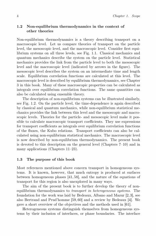
1.3 The purpose of this book
Most references mentioned above concern transport in homogeneous sys-tems. It is known, however, that much entropy is produced at surfacesbetween homogeneous phases [41, 58], and the nature of the equations oftransport for this region is also unexplored in many ways.
The aim of the present book is to further develop the theory of non-equilibrium thermodynamics to transport in heterogeneous systems. Thefoundation for the work was laid by Bedeaux, Albano and Mazur [2,3], seealso Bertrand and Prud’homme [59, 60] and a review by Bedeaux [4]. Wegave a short overview of the objectives and the methods used in [61].
Heterogeneous systems distinguish themselves from homogeneous sys-tems by their inclusion of interfaces, or phase boundaries. The interface

1.3. The purpose of this book 5
Classical mechanics Statistical mechanics
Pair correlation functionMaxwell distribution
Structure factor
Equation of state
Ensemble theoryGibbs
S = S(U,V,N)
Particle level Particle level
Mesoscopic level Macroscopic level
BoltzmannNewton
Quantum mechanicsSchrodinger
Equilibrium correlationfunctions
Phase equilibria
ThermodynamicsIntegral
identities
Schrodinger:::
BS = k lnW
Figure 1.1 Theories for equilibrium systems on the particle-, mesoscopic- andmacroscopic level.
Classical mechanics
Particle level Particle level
Quantum mechanics
Kuborelations
Time dependent
statistical mechanics
Liouville equationLiouville von Neumann
equation
thermodynamics
..
Mesoscopic level Macroscopic level
Fokker Planck equationLangevin equation
Navier Stokes equations
Maxwell Stefan equations
Onsager relationsLinear flux force relations
correlation functionsKinetic theory
Master equation
Schrodinger
Newton
Boltzmann equation
Non equilibrium
Non equilibrium
Figure 1.2 Theories for non-equilibrium systems on the particle-, mesoscopic-and macroscopic level.

6 Chapter 1. Scope
can, according to Gibbs [62], be regarded as a separate two-dimensionalthermodynamic system within the larger three-dimensional system. Thisimplies the introduction of excess densities along the surface. The purposeof this book is to extend the work of Gibbs to non-equilibrium systems. Thisimplies the introduction of not only time dependent excess densities for thesurface but also of time dependent excess fluxes along the surface. In thismanner we shall describe transport of heat, mass and charge and chemicalreactions in heterogeneous systems.
Isotropic homogeneous systems have no coupling between vectorial phe-nomena (transport of heat, mass and charge) and scalar phenomena (chem-ical reactions). In these systems, the two classes can therefore be dealt withseparately [20]. In a two-dimensional surface, all transport processes in thedirection normal to the surface become scalar. This means that couplingcan occur between transport of heat, mass and charge in that direction, andchemical reactions. The coupling is typical for electrode surfaces, phasetransitions and membrane surfaces, and the coupling coefficients are oftenlarge. This coupling is special for heterogeneous systems, and is studied inmany examples throughout the book. The flux equations at the surfacesgive jumps in intensive variables, and define in this manner boundary condi-tions for integration through the surface. Such integrations can be found inseveral chapters. Electric potential changes shall be described by a changein the electromotive force, or in the electrochemical potential difference ofthe ion, which is reversible to the electrode pair [23, 27, 63].
With a short exception for the contact line (Chapter 6), we shall notconsider transport along the surface. While this is an extremely impor-tant phenomenon, it would be too much new material to cover. We fur-ther neglect viscous phenomena. We shall not deal with systems whereit is necessary to take fluxes along as variables [64]. We shall not intro-duce internal variables [45–47]. The transports considered in this bookare almost all in the direction normal to the surface, and are thereforeone-dimensional.
The book aims to make clear that non-equilibrium thermodynamics isa systematic theory that rests on sound assumptions. The assumption oflocal equilibrium is valid for systems in large gradients [65, 66], includingsurfaces [40, 67, 68], and does not depend on stationary state conditions,constant external forces, absence of electric polarization or isotropy, as hasbeen claimed, see for instance [22].

Chapter 2
Why Non-Equilibrium
Thermodynamics?
This chapter explains what the field of non-equilibrium thermodynamicsadds to the analysis of common scientific and engineering problems. Accu-rate and reliable flux equations can be obtained. Experiments can be welldefined. Knowledge of transport properties gives information on the sys-tem’s ability to convert energy.
The most common industrial and living systems have transport of heat,mass and charge, alone or in combination with a chemical reaction. Theprocess industry, the electrochemical industry, biological systems, as well aslaboratory experiments, all concern heterogeneous systems, which are notin global equilibrium. There are four major reasons why non-equilibriumthermodynamics is important for such systems. In the first place, the the-ory gives an accurate description of coupled transport processes. In thesecond place, a framework is obtained for the definition of experiments.In the third place; the theory quantifies not only the entropy that is pro-duced during transport, but also the work that is done and the lost work.Last but not least, this theory allows us to check that the thermody-namic equations we use to model our system are in agreement with thesecond law.
The aim of this book is to give a systematic description of transport inheterogeneous systems. Non-equilibrium thermodynamics has so far mostlybeen used in science [20,21,27]. Accurate expressions for the fluxes are nowrequired also in engineering [29, 42, 69]. In order to see immediately whatnon-equilibrium thermodynamics can add to the description of real systems,we compare simple flux equations to flux equations given by non-equilibriumthermodynamics in the following four sections.
7
8 Chapter 2. Why Non-Equilibrium Thermodynamics?
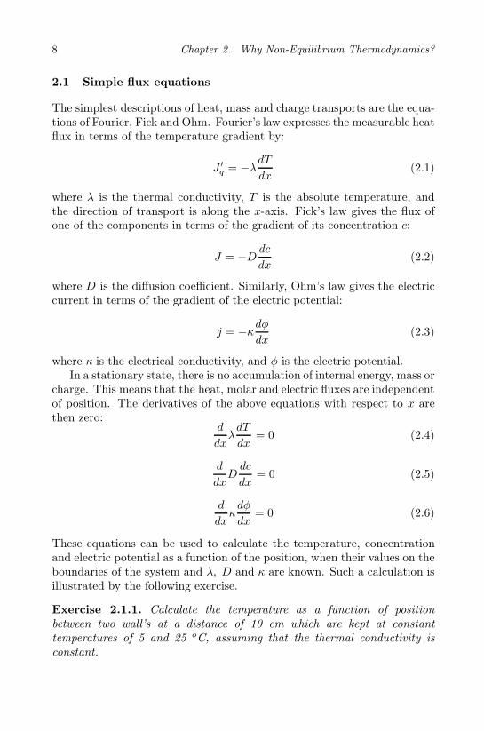
2.1 Simple flux equations
The simplest descriptions of heat, mass and charge transports are the equa-tions of Fourier, Fick and Ohm. Fourier’s law expresses the measurable heatflux in terms of the temperature gradient by:
J ′q = −λdT
dx(2.1)
where λ is the thermal conductivity, T is the absolute temperature, andthe direction of transport is along the x-axis. Fick’s law gives the flux ofone of the components in terms of the gradient of its concentration c:
J = −D dc
dx(2.2)
where D is the diffusion coefficient. Similarly, Ohm’s law gives the electriccurrent in terms of the gradient of the electric potential:
j = −κdφdx
(2.3)
where κ is the electrical conductivity, and φ is the electric potential.In a stationary state, there is no accumulation of internal energy, mass or
charge. This means that the heat, molar and electric fluxes are independentof position. The derivatives of the above equations with respect to x arethen zero:
d
dxλdT
dx= 0 (2.4)
d
dxDdc
dx= 0 (2.5)
d
dxκdφ
dx= 0 (2.6)
These equations can be used to calculate the temperature, concentrationand electric potential as a function of the position, when their values on theboundaries of the system and λ, D and κ are known. Such a calculation isillustrated by the following exercise.
Exercise 2.1.1. Calculate the temperature as a function of positionbetween two wall’s at a distance of 10 cm which are kept at constanttemperatures of 5 and 25 oC, assuming that the thermal conductivity isconstant.
2.2. Flux equations with coupling terms 9
• Solution: According to Eq. (2.4), d2T/dx2 = 0. The general solutionof this equation is T (x) = a+ bx. The constants a and b follow fromthe boundary condition. We have T (0) = 5oC and T (10) = 25oC. Itfollows that T (x) = (5 + 2x)oC.
Equations (2.1)–(2.3) describe a pure degradation of thermal, chemical andelectrical energy. In reality there is also conversion between the energyforms. For an efficient exploitation of energy resources, such a conversion isessential. This is captured in non-equilibrium thermodynamics by the so-called coupling coefficients. Mass transport occurs, for instance, not onlybecause dc/dx 6= 0, but also because dT/dx 6= 0 or dφ/dx 6= 0.
Chemical and mechanical engineers need theories of transport for in-creasingly complex systems with gradients in pressure, concentration andtemperature. Simple vectorial transport laws have long worked well in engi-neering, but there is now an increasing effort to be more precise. The booksby Taylor and Krishna [69], Kuiken [31] and by Cussler [70], which useMaxwell–Stefan’s formulation of the flux equations, are important books inthis context. A need for more accurate flux equations in modeling [42, 69]makes non-equilibrium thermodynamics a necessary tool.
2.2 Flux equations with coupling terms
Many natural and man-made processes are not adequately described bythe simple flux equations given above. There are, for instance, always largefluxes of mass and heat that accompany charge transport in batteries andelectrolysis cells. The resulting local cooling in electrolysis cells may lead tounwanted freezing of the electrolyte. Electrical energy is frequently used totransport mass in biological systems. Large temperature gradients acrossspace ships have been used to supply electric power to the ships. Saltconcentration differences between river water and sea water can be used togenerate electric power. Pure water can be generated from salt water byapplication of pressure gradients. In all these more or less randomly chosenexamples, one needs transport equations that describe coupling betweenvarious fluxes. The flux equations given above become too simple.
Non-equilibrium thermodynamics introduces coupling among fluxes.Coupling means that transport of mass will take place in a system notonly when the gradient in the chemical potential is different from zero, butalso when there are gradients in temperature or electric potential. Couplingbetween fluxes can describe the phenomena mentioned above.
For example, in a bulk system with transport of heat, mass, and electriccharge in the x-direction, we shall find that the linear relations (1.2) take
10 Chapter 2. Why Non-Equilibrium Thermodynamics?
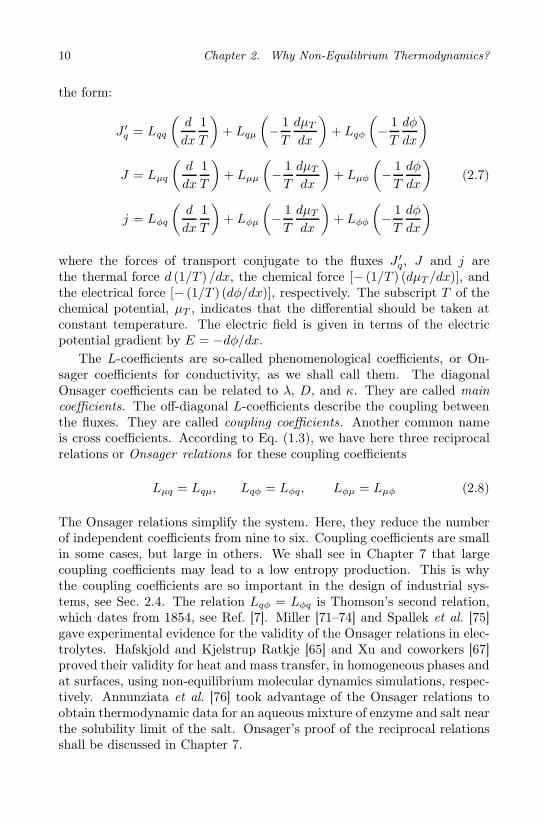
the form:
J ′q = Lqq
(d
dx
1
T
)+ Lqµ
(− 1
T
dµT
dx
)+ Lqφ
(− 1
T
dφ
dx
)
J = Lµq
(d
dx
1
T
)+ Lµµ
(− 1
T
dµT
dx
)+ Lµφ
(− 1
T
dφ
dx
)
j = Lφq
(d
dx
1
T
)+ Lφµ
(− 1
T
dµT
dx
)+ Lφφ
(− 1
T
dφ
dx
)
(2.7)
where the forces of transport conjugate to the fluxes J ′q, J and j are
the thermal force d (1/T )/dx, the chemical force [− (1/T ) (dµT /dx)], andthe electrical force [− (1/T ) (dφ/dx)], respectively. The subscript T of thechemical potential, µT , indicates that the differential should be taken atconstant temperature. The electric field is given in terms of the electricpotential gradient by E = −dφ/dx.
The L-coefficients are so-called phenomenological coefficients, or On-sager coefficients for conductivity, as we shall call them. The diagonalOnsager coefficients can be related to λ, D, and κ. They are called maincoefficients. The off-diagonal L-coefficients describe the coupling betweenthe fluxes. They are called coupling coefficients. Another common nameis cross coefficients. According to Eq. (1.3), we have here three reciprocalrelations or Onsager relations for these coupling coefficients
Lµq = Lqµ, Lqφ = Lφq, Lφµ = Lµφ (2.8)
The Onsager relations simplify the system. Here, they reduce the numberof independent coefficients from nine to six. Coupling coefficients are smallin some cases, but large in others. We shall see in Chapter 7 that largecoupling coefficients may lead to a low entropy production. This is whythe coupling coefficients are so important in the design of industrial sys-tems, see Sec. 2.4. The relation Lqφ = Lφq is Thomson’s second relation,which dates from 1854, see Ref. [7]. Miller [71–74] and Spallek et al. [75]gave experimental evidence for the validity of the Onsager relations in elec-trolytes. Hafskjold and Kjelstrup Ratkje [65] and Xu and coworkers [67]proved their validity for heat and mass transfer, in homogeneous phases andat surfaces, using non-equilibrium molecular dynamics simulations, respec-tively. Annunziata et al. [76] took advantage of the Onsager relations toobtain thermodynamic data for an aqueous mixture of enzyme and salt nearthe solubility limit of the salt. Onsager’s proof of the reciprocal relationsshall be discussed in Chapter 7.

2.3. Experimental designs and controls 11
2.3 Experimental designs and controls
The importance of equilibrium thermodynamics for the design of exper-iments is well known. The definition of, say, a partial molar property,explains what shall be varied, and what shall be kept constant in the ex-perimental determination of the quantity. Also, there are relations be-tween thermodynamic variables that offer alternative measurements. Forinstance, the enthalpy of evaporation can be measured in a calorimeter, butit can also be determined by finding the vapor pressure of the evaporatinggas as a function of temperature.
Non-equilibrium thermodynamics is in a similar way, instrumental fordesign of experiments that aim to find transport properties, cf. Chapter 20.To see this, consider the exercise below.
Exercise 2.3.1. Find the electric current in terms of the electric field,E = −dφ/dx, using Eq. (2.7), in a system where there is no transport ofheat and mass, J ′
q = J = 0.
• Solution: It follows from Eqs. (2.7a) and (2.7b) that
Lqq
T
d
dxT + Lqµ
dµT
dx= LqφE and
Lµq
T
d
dxT + Lµµ
dµT
dx= LµφE
Solving these equations, using the Onsager relations, one finds
1
T
d
dxT =
LqφLµµ − LµφLqµ
LqqLµµ − L2qµ
E anddµT
dx=LqqLµφ − LµqLqφ
LqqLµµ − L2qµ
E
Substitution into Eq. (2.7c) then gives
j =E
T
[Lφφ − Lφq
LqφLµµ − LµφLqµ
LqqLµµ − L2qµ
− LφµLqqLµφ − LµqLqφ
LqqLµµ − L2qµ
]
This exercise shows that the electric conductivity, that one measures asthe ratio of measured values of j and E, is not necessarily given by Lφφ/Tas one might have thought, considering Eq. (2.7c). In the stationary state,the coupling coefficients lead to temperature and chemical potential gradi-ents, which again affect the electric current. Mathematically speaking, theelectric conductivity then becomes a combination of the conductivity of ahomogeneous conductor, found if one could measure with zero chemical po-tential and temperature gradients, and additional terms. The combinationof coefficients divided by the temperature, is the stationary state conductiv-ity. The stationary state electric conductivity, measured with J ′
q = J = 0,is experimentally distinguishable from the Ohmic electric conductivity of

12 Chapter 2. Why Non-Equilibrium Thermodynamics?
the homogeneous conductor, measured with dT/dx = dµT /dx = 0. Non-equilibrium thermodynamics helps define conditions that give well definedexperiments.
One important practical consequence of the Onsager relations is to offeralternative measurements for the same property. For instance, if it is dif-ficult to measure the coefficient Lqφ, one may rather measure Lφq [77–80].A valuable consistency check for measurements is provided if one measuresboth coupling coefficients in the relation. So, similar to the situation inequilibrium, also the non-equilibrium systems have possibilities for controlof internal consistency.
2.4 Entropy production, work and lost work
Non-equilibrium thermodynamics is probably the only method that can beused to assess how energy resources are exploited within a system. Thisis because the theory deals with energy conversion on the local level in asystem, i.e. at the electrode surface [81] or in a biological membrane [52].By integration to the system level, we obtain a link to exergy analysis [82].To see the relation between non-equilibrium thermodynamics and exergyanalysis, consider again the thermodynamic fluxes and forces, derived fromthe local entropy production
σ =∑
i
JiXi ≥ 0 (2.9)
The total entropy production is the integral of σ over the volume V of thesystem
dSirr
dt=
∫σdV (2.10)
The quantity dSirr/dt makes it possible to calculate the energy dissipatedas heat or the lost work in a system (see below).
In an industrial plant, the materials undergo certain transformationsin a time interval dt. Materials are taken in and are leaving the plant atthe conditions of the environment. The environment is a natural choice asframe of reference for the analysis. It has constant pressure, p0 (1 bar), andconstant temperature, T0 (for instance 298 K) and some average composi-tion that needs to be defined. The first law of thermodynamics gives theenergy change of the process per unit of time:
dU
dt=dQ
dt− p0
dV
dt+dW
dt(2.11)
Here dQ/dt is the rate that heat is delivered to the materials, p0dV/dt is thework that the system does per unit of time by volume expansion against the

2.4. Entropy production, work and lost work 13
dW/dt
dU/dt
T
dQ /dt
0 0
0
p
Figure 2.1 A schematic illustration of thermodynamic variables that areessential for the lost work in an industrial plant.
pressure of the environment, and dW/dt is the work done on the materialsper unit of time.
The minimum work needed to perform a process, is the least amount ofenergy that must be supplied, when at the conclusion of the process, theonly systems which have undergone any change are the process materials[83]. To see this, we replace dQ/dt by minus the heat delivered to theenvironment per unit of time, dQ/dt = −dQ0/dt:
dU
dt= −dQ0
dt− p0
dV
dt+dW
dt(2.12)
The second law givesdS
dt+dS0
dt≥ 0 (2.13)
where dS/dt is the rate of entropy change of the process materials anddS0/dt is the rate of entropy change in the environment. For a completelyreversible process the sum of these entropy rate changes is zero. For anon-equilibrium process, the sum is the total entropy production, dSirr/dt,
dSirr
dt≡ dS
dt+dS0
dt≥ 0 (2.14)
The entropy change in the surroundings is dS0/dt = (dQ0/dt) /T0. By in-troducing dQ0/dt into the expression for the entropy production, and com-bining the result with the first law, we obtain after some rearrangement:
dW
dt= T0
dSirr
dt+dU
dt+ p0
dV
dt− T0
dS
dt(2.15)
14 Chapter 2. Why Non-Equilibrium Thermodynamics?
The left hand side of this equation is the work that is needed to accomplishthe process with a particular value of the entropy production, dSirr/dt.Since dSirr/dt ≥ 0, the ideal (reversible) work requirement of this processis:
dWideal
dt=dU
dt+ p0
dV
dt− T0
dS
dt(2.16)
We see that dS/dt changes the ideal work. By comparing Eqs. (2.15) and(2.16), we see that T0(dSirr/dt) is the additional quantity of work per unitof time that must be used in the actual process, compared to the work inan ideal (reversible) process. Thus, T0(dSirr/dt) is the wasted or lost workper unit of time:
dWlost
dt= T0
dSirr
dt(2.17)
The lost work is the energy dissipated as heat in the surroundings. Therelation is called the Gouy–Stodola theorem [84, 85]. The right hand sideof Eq. (2.16) is also called the time rate of change of the availability orthe exergy [62, 82]. We shall learn how to derive σ in subsequent chap-ters. One aim of the process operator or designer should be to minimizedWlost/dt [86], which is equivalent to entropy production minimization, seeRef. [85] page 227 and Ref. [29] Chapter 6. Knowledge about the sourcesof entropy production is central for work to improve the energy efficiencyof processes. In a recent book “Elements of irreversible thermodynamicsfor engineers” [28, 29], we discussed how irreversible thermodynamics canbe used to map the lost work in an industrial process. The aluminiumelectrolysis was used as an example to illustrate the importance of sucha mapping. Furthermore the first steps in a systematic method for theminimization of entropy production was described, with its basis in non-equilibrium thermodynamics. Second law optimization [85, 87–92] in me-chanical and chemical engineering may become increasingly important inthe design of systems that waste less work. Non-equilibrium thermody-namics will play a unique role in this context. For details on how to mapthe second law efficiency of an industrial system or how to systematicallyimprove this efficiency, we refer to Bejan [84,85] and to the book “Elementsof irreversible thermodynamics for engineers” [28, 29].
2.5 Consistent thermodynamic models
The entropy balance of the system and the expression for the entropy pro-duction can be used for control of the internal consistency of the thermo-dynamic description. The change of the entropy in a volume element in ahomogeneous phase is given by the flow of entropy in and out of the volume

2.5. Consistent thermodynamic models 15
element and by the entropy production inside the element:
∂s
∂t= − ∂
∂xJs + σ (2.18)
where we take the entropy flux in the x-direction. In the stationary state,there is no change in the system’s entropy and
σ =∂
∂xJs (2.19)
By integrating over the system’s extension, keeping its cross-sectional areaΩ constant, we obtain
dSirr
dt= Ω(Jo
s − J is) (2.20)
The left hand side is obtained from σ, which is a function of transportcoefficients, fluxes and forces, Eqs. (1.1)–(1.3). The right hand side of thisequation, the difference in the entropy flows, Jo
s −J is, can be calculated from
knowledge of the heat flux, and of the entropy carried by components intothe surroundings. These quantities do not depend on the system’s transportproperties. The two calculations must give the same result. Chapter 19gives an example of such a comparison. Other examples were given byKjelstrup et al. [29], see also Zvolinschi et al. [92].

This page intentionally left blankThis page intentionally left blank

Chapter 3
Thermodynamic Relations for
Heterogeneous Systems
This chapter gives thermodynamic relations for heterogeneous systems thatare in global equilibrium, and discusses the meaning of local equilibrium inhomogeneous phases, at surfaces and along three phase contact lines.
The heterogeneous systems that are treated in this book exchange heat,mass and charge with their surroundings. The systems have homogeneousphases separated by an interfacial region. They are electroneutral, butpolarizable. The words surface and interface will be used interchangeablyto indicate the interfacial region. Gibbs [62] calls the interfacial region“the surface of discontinuity”. Thermodynamic relations for homogeneousphases, as well as for surfaces, are mandatory for the chapters to follow.Such equations are therefore presented here [62,93]. Equations for the threephase contact line are also given, but are less central. The equations aregiven first for systems that are in global equilibrium, and next for non-equilibrium systems where only local equilibrium applies.
A thermodynamic description of equilibrium surfaces in terms of excessdensities was constructed by Gibbs [62]. This description treats the surfaceas an autonomous thermodynamic system. We use this description in termsof excess densities as our basis also in non-equilibrium systems. This impliesfor instance that the surface has its own temperature. All excess densities ofa surface depend on this temperature alone and not on the temperatures inthe adjacent phases∗. We present evidence for this assumption using non-equilibrium molecular dynamics simulations (Chapter 22) and the squaregradient model of van der Waals (Chapter 23).
∗This property of the surface has been defended by some authors [94,95], but rejectedby others [96].
17

18 Chapter 3. Thermodynamic Relations for Heterogeneous Systems
We extend Gibbs’ formulation for the surface to the contact line. Equi-librium relations for the three phase contact lines can be formulated forexcess line densities. The line, described in this manner, is also an au-tonomous thermodynamic system.
3.1 Two homogeneous phases separated by a surface in
global equilibrium
Consider two phases of a multi-component system in equilibrium with eachother. The system is polarizable in an electric field. The last propertyis relevant for electrochemical systems. In systems that transport heatand mass only, this property is not relevant. The homogeneous phases, iand o, have their internal energies, U i and Uo, entropies, Si and So, molenumbers, N i
j and Noj of the components j (see for instance [97]), and their
polarizations in the direction normal to the surface, Pi and P
o. For thetotal system, we have:
U = U i + U s + Uo (3.1)
The internal energy for the total system, U, minus the sum of the two bulkvalues gives the internal energy of the interfacial region U s [62,93]. For theentropy, the mole numbers and the polarization, we similarly have:
S = Si + Ss + So
Nj = N ij +N s
j +Noj
P = Pi + P
s + Po
(3.2)
The surface consists of layer(s) of molecules or atoms, with negligible vol-ume, so
V = V i + V o (3.3)
The surface area, Ω, is an extensive variable of the surface, comparable tothe volume as a variable of a homogeneous phase. The surface tension, γ,plays a similar role for the surface as the pressures, pi and po, do for thehomogeneous phases.
The polarizations of the homogeneous phases can be expressed in termsof the polarization densities (polarization per unit of volume), P i and P o,by
Pi = P iV i and P
o = P oV o (3.4)
The polarization of the surface can similarly be expressed as the polarizationper unit of surface area, P s:
Ps = P sΩ (3.5)

3.1. Two homogeneous phases separated by a surface in global equilibrium 19
The polarization density is particular for both homogeneous phases andthe surface. The system may contain polarizable molecules (apolar), polarmolecules and free charges. An electric field leads to polarization of theapolar molecules and to orientation of the polar molecules. Furthermore, itleads to a redistribution of free charges. In all cases, polarization occurs ina manner that keeps homogeneous phases and surfaces electroneutral. Fora double layer, we define a surface polarization. For a conductor, we definea polarization density. The divergence of the polarization of a conductorequals the charge distribution, but the induced charge distribution in anelectric field integrates to zero net charge.
In this book, we restrict ourselves to surfaces that are planar and con-tact lines that are straight. From the second Maxwell equation, and thecondition of electroneutrality, we have
d
dxD = 0 (3.6)
where D is the displacement field normal to the surface. The normal com-ponent of the displacement field across an electroneutral surface is contin-uous, and has accordingly no contribution for the surface; Ds = 0. Thenormal component of the displacement field is therefore constant through-out a heterogeneous system. Its value can be controlled from the outsideby putting the system between a parallel plate capacitor. In this book, wedo not consider electric potential gradients along the surface. Assumingthe system furthermore to be invariant for translations along the surface,rotations around a normal on the surface and reflection in planes normalto the surface, it follows that electric fields, displacement fields and polar-izations are normal to the surface. The displacement field is related to theelectric fields in the two phases by
D = ε0Ei + P i = εiE
i and D = ε0Eo + P o = εoE
o (3.7)
where εi and εo are the dielectric constants of the phases i and o respectively.Furthermore, ε0 is the dielectric constant of vacuum. A similar relation canbe written for the electric field of the surface
Ds = 0 = ε0Es + P s → P s = −ε0Es (3.8)
For more precise definitions of the interfacial densities we refer to the nextsection and to Sec. 5.2. For an in-depth discussion of the excess polarizationand electric field, we refer to the book by Bedeaux and Vlieger, OpticalProperties of Surfaces [5, 6].
Remark 3.1. The surface polarization is equal to minus ε0 times the ex-cess electric field of the surface. This follows from the following argument:

20 Chapter 3. Thermodynamic Relations for Heterogeneous Systems
The displacement field is the sum of ε0 times the electric field plus the po-larization density. The displacement field is continuous through the surface.The sum of the electric field times ε0 plus the surface polarization densitymust therefore be zero.
For heterogeneous, polarizable systems, we can then write the internalenergy as a total differential of the extensive variables S, Nj, V , Ω, P
i, Po
and Ps:
dU = TdS − pdV + γdΩ +
n∑
j=1
µjdNj +Deqd
(P
i
εi+
Ps
ε0+
Po
εo
)(3.9)
where Deq is the displacement field that derives from a reversible trans-formation. This is the Gibbs equation [62], extended with terms due topolarization. By integrating with constant intensive variables, the energyof the system becomes
U = TS − pV + γΩ +
n∑
j=1
µjNj +Deq
(P
i
εi+
Ps
ε0+
Po
εo
)(3.10)
Since we are dealing with state functions, this result is generally valid. Thecontributions to the internal energy from the polarization are DeqP
i/εi andDeqP
o/εo in the homogeneous phases and DeqPs/ε0 [3] for the surface.
Remark 3.2. The contributions to the total polarization, i.e. from polar-izable molecules, from polar molecules and from free charges, have verydifferent relaxation times. They should therefore be counted as separatecontributions P
α =∑
k Pαk , where α equals i, o or s. The corresponding
equilibrium displacement fields, Deq,k, found from a reversible transforma-tion, are also different for the different contributions to the polarization.We shall not make the formulae more cumbersome by distinguishing thesedifferent contributions.
The surface tension is, like the pressure, a function of T , µj , and Deq.The most directly observable effect of the surface tension is found whenthe interface between two phases is curved. Consider for instance a spher-ical bubble in a liquid. The pressure inside the bubble is higher than thepressure outside. The same is true for a liquid droplet in air. The pressuredifference, called the capillary pressure, is given in terms of the surface ten-sion by 2γ/R , where R is the radius of the droplet. The capillary pressureis the reason why water rises in a capillary. The following exercise demon-strates that the energy represented by a surface can be compared to theenergy of a homogeneous phase.

3.1. Two homogeneous phases separated by a surface in global equilibrium 21
Exercise 3.1.1. Use the expression for the capillary pressure to derive aformula for the rise of liquid in a capillary as function of the diameter dof the capillary. The liquid wets the surface. Calculate the capillary rise ofwater in a capillary with a diameter of a micron. The surface tension ofwater is γw = 75 × 10−3 N/m.
• Solution: If the diameter of the capillary is not too large, and whenthe liquid wets the surface, the interface between the water and theair is a half sphere with radius d/2. This gives a capillary pressureof 4γ/d. This would cause an under-pressure in the liquid below thesurface. In order to have a normal atmospheric pressure at the bottomof the capillary, the water rises until the weight of the column gives thecapillary pressure. This implies that π(d/2)2hgρ/π(d/2)2 = hgρ =4γ/d where h is the height of the column, ρ is the density in kg/m3
of water and g is the acceleration of gravity. The capillary rise istherefore h = 4γ/dgρ. In a capillary with a diameter of a micron, thecapillary rise of water is 30 m.
In this book we restrict ourselves to surfaces that are flat. The equilibriumpressure is therefore always constant throughout the system, pi = po = p.
The Gibbs equation (3.9) gives the energy of both homogeneous phasesplus the surface. We need also equations for the separate homogeneousphases and for the surface alone. With Eqs. (3.1)–(3.3), we have for phasei:
dU i = TdSi − pdV i +
n∑
j=1
µjdNij +Deqd
Pi
εi(3.11)
This is the Gibbs equation for phase i. We integrate the equation forconstant composition, temperature, pressure and displacement field. Thisgives:
U i = TSi − pV i +
n∑
j=1
µjNij +Deq
Pi
εi(3.12)
The energy is a state function, so the result is generally valid (compareEq. (3.10)). By differentiating this expression and subtracting Eq. (3.11),we obtain Gibbs–Duhem’s equation:
0 = SidT − V idp+
n∑
j=1
N ijdµj +
Pi
εidDeq (3.13)
Similar equations can be written for phase o.

22 Chapter 3. Thermodynamic Relations for Heterogeneous Systems
The Gibbs equation for the surface is likewise:
dU s = TdSs + γdΩ +n∑
j=1
µjdNsj +
(Deq
ε0
)dPs (3.14)
By integration for constant surface tension, temperature, composition anddisplacement field, we obtain
U s = TSs + γΩ +
n∑
j=1
µjNsj +
(Deq
ε0
)P
s (3.15)
Gibbs–Duhem’s equation for the surface follows by differentiating this equa-tion and subtracting Eq. (3.14):
0 = SsdT + Ωdγ +
n∑
j=1
N sjdµj + P
sd
(Deq
ε0
)(3.16)
The thermodynamic relations for the autonomous surface, Eqs. (3.14)-(3.16), are identical in form to the thermodynamic relations for the ho-mogeneous phases, compare Eqs. (3.11)–(3.13).
Global equilibrium in a heterogeneous, polarizable system in a displace-ment field can now be defined. The chemical potentials and the temperatureare constant throughout the system
µij = µs
j = µoj = µj
T i = T s = T o = T(3.17)
Furthermore, the normal component of the pressure and of the displacementfield are the same in the adjacent homogeneous phases:
pi = po = p and Deq constant (3.18)
For curved surfaces the normal component of the pressure is not constantand we refer to Blokhuis, Bedeaux and Groenewold [98–103].
The surface energy, and therefore also the surface entropy and surfacemole numbers, have so far been defined from the total values minus thebulk values. We shall see in Sec. 3.3, how more direct definitions can beformulated.
3.2 The contact line in global equilibrium
Consider three phases of a multi-component system in equilibrium with eachother. The three surfaces separating these phases come together in a contact

3.3. Defining thermodynamic variables for the surface 23
line. For simplicity, we assume that the contact line is not polarizable.In the previous section we have seen that the thermodynamic relationsfor an autonomous surface has the same form as for homogeneous phases.The same is true for the autonomous three-phase contact line. The Gibbsequation for the contact line is:
dU c = TdSc + γcdL+n∑
j=1
µjdNcj (3.19)
Superscript c indicates a contribution of the contact line, γc is the linetension and L is the length of the line. The curvature of the line is assumedto be negligible, so that there are no contributions to dU c from changes inthe curvature. By integration for constant line tension, temperature andcomposition, we obtain
U c = TSc + γcL+
n∑
j=1
µjNcj (3.20)
The line energy, and therefore also the line entropy and the line mole num-bers, have here been defined as the total values minus the bulk and thesurface values.
Gibbs–Duhem’s equation for the line follows by differentiating this equa-tion and subtracting Eq. (3.19):
0 = ScdT + Ldγc +n∑
j=1
N cj dµj (3.21)
When the contact line is part of a heterogeneous system in global equilib-rium, the chemical potentials and the temperature are constant throughoutthe system. For the contact line, we therefore also have
µcj = µj and T c = T (3.22)
More direct definitions of thermodynamic properties of the line, can beobtained, following the procedure for the surface in the next section.
3.3 Defining thermodynamic variables for the surface
The relations for global equilibrium cannot be used to describe systems withgradients in µ, p, T or the electric field. We must therefore also formulaterelations for local equilibrium. We need local forms of the Gibbs and Gibbs–Duhem equations. These will be given after we have first defined the surfacevariables.

24 Chapter 3. Thermodynamic Relations for Heterogeneous Systems
Figure 3.1 Variation in the molar density of a fluid if we go from the gas tothe liquid state. The vertical lines indicate the extension of the surface. Thescale of the x-axis is measured in nanometer.
An interface is the thin layer between two homogeneous phases. Werestrict ourselves to flat surfaces, that are perpendicular to the x-axis. Thethermodynamic properties of the interface shall now be given by the valuesof the excess densities of the interface. The value of these densities andthe location of the interface will be defined through the example of a gas-liquid interface. We shall correspondingly indicate these phases with thesuperscripts g and l.
Figure 3.1 shows the variation in concentration of A, in a mixture ofseveral components, as we go from the gas to the liquid phase. The surfacethickness is usually a fraction of a nm. The x-axis of Fig. 3.1 has coordinatesin nm, it has a molecular scale. A continuous variation in the concentrationis seen. Gibbs [62] defined the surface of discontinuity as a transition regionwith a finite thickness bounded by planes of similarly chosen points. In thefigure two such planes are indicated by vertical lines. The position a isthe point in the gas left of the closed surface where cA(x) starts to differfrom the concentration of the gas, cgA, and the position b is the point inthe liquid right of the closed surface, where cA(x) starts to differ from theconcentration of the liquid, clA. The surface thickness is then δ = b − a.It refers to component A. Other components may yield somewhat differentplanes.
Gibbs defined the dividing surface as “a geometrical plane, goingthrough points in the interfacial region, similarly situated with respect to

3.3. Defining thermodynamic variables for the surface 25
conditions of adjacent matter”. Many different planes of this type can bechosen. While the position of the dividing surface depends on this choice;it is normally somewhere between the vertical lines in Fig. 3.1. The planesthat separate the closed surface from the homogeneous phases are parallelto the dividing surface. The continuous density, integrated over δ, givesthe excess surface concentration of the component A as a function of theposition, (y, z), along the surface:
ΓA(y, z) =
∫ b
a
[cA(x, y, z) − cgA(a, y, z)θ(d− x) − clA(b, y, z)θ(x− d)
]dx
(3.23)where d is the position of the dividing surface. The surface concentrationis often called the adsorption (in mol/m2). The Heaviside function, θ,is by definition unity when the argument is positive and zero when theargument is negative. It is common to choose d between a and b. Otherexcess variables than ΓA are defined similarly. All excess properties of asurface can be given by integrals like Eq. (3.23). The excess variables arethe extensive variables of the surface. They describe how the surface differsfrom adjacent homogeneous phases.
Remark 3.3. It is clear from Fig. 3.1 that one may shift the position ato the left and b to the right without changing the adsorption. This showswhy the precise location of a and b is not important for the value of theadsorption.
Gibbs defined the excess concentrations for global equilibrium. Equa-tion (3.23) will be used in this book also for systems which are not in globalequilibrium. In fact, ΓA, cA, cgA and clA as well as a, b and d, may all dependon the time. For ease of notation this was not explicitly indicated.
The equimolar surface of component A is a special dividing surface. Thelocation is such that the surplus of moles of the component on one side ofthe surface is equal to the deficiency of moles of the component on the otherside of the surface, see Fig. 3.2. The position, d, of the equimolar surfaceobeys:
∫ d
a
[cA(x, y, z) − cgA(a, y, z)]dx = −∫ b
d
[cA(x, y, z) − clA(b, y, z)
]dx
(3.24)According to Eqs. (3.23) and (3.24), ΓA = 0, when the surface has thisposition, see Fig. 3.2. The shaded areas in the figure are equal. In amulti-component systems, each component has its “equimolar” surface, butwe have to make one choice for the position of the dividing surface. Weusually choose the position of the surface as the equimolar surface of the
26 Chapter 3. Thermodynamic Relations for Heterogeneous Systems
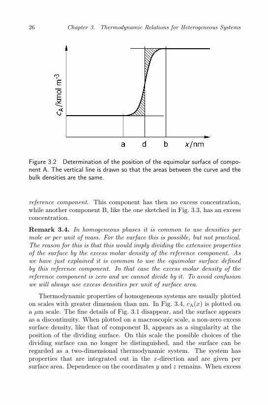
Figure 3.2 Determination of the position of the equimolar surface of compo-nent A. The vertical line is drawn so that the areas between the curve and thebulk densities are the same.
reference component. This component has then no excess concentration,while another component B, like the one sketched in Fig. 3.3, has an excessconcentration.
Remark 3.4. In homogeneous phases it is common to use densities permole or per unit of mass. For the surface this is possible, but not practical.The reason for this is that this would imply dividing the extensive propertiesof the surface by the excess molar density of the reference component. Aswe have just explained it is common to use the equimolar surface definedby this reference component. In that case the excess molar density of thereference component is zero and we cannot divide by it. To avoid confusionwe will always use excess densities per unit of surface area.
Thermodynamic properties of homogeneous systems are usually plottedon scales with greater dimension than nm. In Fig. 3.4, cA(x) is plotted ona µm scale. The fine details of Fig. 3.1 disappear, and the surface appearsas a discontinuity. When plotted on a macroscopic scale, a non-zero excesssurface density, like that of component B, appears as a singularity at theposition of the dividing surface. On this scale the possible choices of thedividing surface can no longer be distinguished, and the surface can beregarded as a two-dimensional thermodynamic system. The system hasproperties that are integrated out in the x -direction and are given persurface area. Dependence on the coordinates y and z remains. When excess

3.3. Defining thermodynamic variables for the surface 27
Figure 3.3 Variation in the density of component B across the surface. Theexcess surface concentration of component B is the integral under the curve inthe figure.
Figure 3.4 The equimolar surface plotted on a micrometer scale appears as ajump between bulk densities.

28 Chapter 3. Thermodynamic Relations for Heterogeneous Systems
surface densities are defined in this manner, the normal thermodynamicrelations, like the first and second laws are valid [62].
Remark 3.5. Excess densities for the surface can be much larger than thetypical value of the integrated quantity times the thickness of the surfaceof discontinuity. The surface tension of a liquid-vapor is for instance afactor between 10 3 to 10 4 larger than the typical pressure of 1 bar times 3Angstroms. This implies that contributions from the surface play a muchmore important role than what the volume of the surface of discontinuitywould suggest.
Van der Waals constructed a continuous model for the liquid-vapor in-terface at equilibrium, around the end of the 19th century [104]. In thismodel one adds to the Helmholtz energy density per unit of volume a con-tribution proportional to the square of the gradient of the density. It istherefore often called the square gradient model. The model was rein-vented by Cahn and Hilliard in 1958 [105]. It has become an importantmodel for studies of the equilibrium structure of the interface [93,102]. Themodel gives a density profile through the closed surface and enables one tocalculate, for instance, the surface tension. An extension of his model tonon-equilibrium systems [106–108] is discussed in Chapter 23. It is foundin the context of this model [107] that the surface, as described by excessdensities, is in local equilibrium.
Exercise 3.3.1. The variation in density of A across a vapor-liquid inter-face between a = 0 and b = 5 nm is given by cA(x) = Cx3 + 50 mol/m3.The vapor density is cgA = 50 mol/m3 and the liquid density is clA = 50000mol/m3. Determine the value of C and the position of the equimolarsurface.
• Solution: The density function at b gives
C(5 × 10⁻⁹)3 + 50 = 5 × 10⁴ ⇒ C = 4 × 1029mol/m6
For the equimolar surface, we have:
∫ d
0
Cx3dx = −∫ b
d
(Cx3 − 49950)dx
⇒ 1
4Cd4 = −1
4C(b4 − d4) + 49950(b− d)

3.4. Local thermodynamic identities 29
This results in the position d = 3.75 nm. The equimolar surface isclose to the liquid side.
3.4 Local thermodynamic identities
In the first section of this chapter, we considered a heterogeneous system inglobal equilibrium. The temperature, the chemical potentials, the pressureand the displacement field were constant throughout the system, Eqs. (3.17)and (3.18). In the previous section, we defined excess densities using ex-pressions that can also be used in non-equilibrium systems. In order to usethe thermodynamic identities from the first section for the excess densities,we need to cast the Gibbs equation and its equivalent forms into a localform.
For the homogeneous phases we introduce the extensive variables perunit of volume. In the i-phase we then have ui = U i/V i, si = Si/V i,cij = N i
j/Vi and the polarization density P i. By dividing Eq. (3.12) by V i
the internal energy density becomes
ui = Tsi − p+n∑
j=1
µjcij +Deq
P i
εi(3.25)
By replacing U i by uiV i etc. in Eq. (3.11), differentiating and usingEq. (3.25), we obtain:
dui = Tdsi +
n∑
j=1
µjdcij +Deqd
P i
εi(3.26)
Gibbs–Duhem’s equation becomes
0 = sidT − dp+
n∑
j=1
cijdµj +P i
εidDeq (3.27)
All quantities in these equations refer now to a local position in space.All expressions for phase i, are also true for phase o. (Replace all the
super- and subscripts i by o). Other thermodynamic relations can also bedefined. We give below the i-phase internal energy, Gibbs energy, Helmholtzenergy, internal energy density, Gibbs energy density and the Helmholtz

30 Chapter 3. Thermodynamic Relations for Heterogeneous Systems
energy density:
U i = TSi − pV i +
n∑
j=1
µjNij +Deq
(P
i/εi)
Gi ≡ U i − TSi + pV i =
n∑
j=1
µjNij +Deq
(P
i/εi)
F i ≡ U i − TSi = −pV i +
n∑
j=1
µjNij +Deq
(P
i/εi)
ui = Tsi − p+
n∑
j=1
µjcij +Deq
(P i/εi
)
gi = ui − Tsi + p =n∑
j=1
µjcij +Deq
(P i/εi
)
f i = ui − Tsi = −p+
n∑
j=1
µjcij +Deq
(P i/εi
)
(3.28)
For the surface, the local variables are given per unit of surface area.These are the excess internal energy density us = U s/Ω, the adsorptionsΓj = N s
j/Ω, the excess entropy density, ss = Ss/Ω, and the surface polar-ization, P s. When we introduce these variables into Eq. (3.14), and useEq. (3.15), we obtain the Gibbs equation for the surface:
dus = Tdss +
n∑
j=1
µjdΓj +DeqdP s
ε0(3.29)
The surface excess internal energy density is
us = Tss + γ +
n∑
j=1
µjΓj +DeqP s
ε0(3.30)
and Gibbs–Duhem’s equation becomes
0 = ssdT + dγ +n∑
j=1
Γjdµj +P s
ε0dDeq (3.31)
We give below the surface internal energy, surface internal energy density,Gibbs equation, Gibbs–Duhem’s equation, surface Gibbs energy density

3.4. Local thermodynamic identities 31
and the surface Helmholtz energy density:
U s = TSs + γΩ +
n∑
j=1
µjNsj +Deq (Ps/ε0)
us = Tss + γ +
n∑
j=1
µjΓj +Deq (P s/ε0)
dus = Tdss +
n∑
j=1
µjdΓj +Deqd (P s/ε0)
0 = ssdT + dγ +
n∑
j=1
Γjdµj + (P s/ε0) dDeq
gs = us − Tss − γ =
n∑
j=1
µjΓj +Deq (P s/ε0)
f s = us − Tss = γ +
n∑
j=1
µjΓj +Deq (P s/ε0)
(3.32)
For the contact line, local variables are given per unit of length. Theseare the excess internal energy density uc = U c/L, the adsorptions Γc
j =N c
j /L and the excess entropy density, sc = Sc/L. When we introduce thesevariables into Eq. (3.19), and use Eq. (3.20), we obtain the Gibbs equationfor the line:
duc = Tdsc +
n∑
j=1
µjdΓcj (3.33)
The contact line excess internal energy density is
uc = Tsc + γc +
n∑
j=1
µjΓcj (3.34)
and Gibbs-Duhem’s equation becomes
0 = scdT + dγc +
n∑
j=1
Γcjdµj (3.35)
Thermodynamic relations for the contact line are given below. We give theline internal energy, line internal energy density, Gibbs equation, Gibbs–Duhem’s equation, contact line Gibbs energy density and the contact line

32 Chapter 3. Thermodynamic Relations for Heterogeneous Systems
Helmholtz energy density:
U c = TSc + γcL+
n∑
j=1
µjNcj
uc = Tsc + γc +
n∑
j=1
µjΓcj
duc = Tdsc +
n∑
j=1
µjdΓcj
0 = scdT + dγc +
n∑
j=1
Γcjdµj
gc = uc − Tsc − γc =
n∑
j=1
µjΓcj
f c = uc − Tsc = γc +
n∑
j=1
µjΓcj
(3.36)
3.5 Defining local equilibrium
We have so far considered global and local thermodynamic relations forheterogeneous systems that are in global equilibrium. We shall now moveone step further and introduce the assumption of local equilibrium. For avolume element in the homogeneous phase i, we say, following Fitts [30],Bedeaux and Kjelstrup [61] and Ortiz and Sengers [109], that there is localequilibrium when the thermodynamic relations (3.25)–(3.27) are valid:
ui(x, t) = T i(x, t)si(x, t) − pi(x, t) +
n∑
j=1
µij(x, t)c
ij(x, t) +Deq(t)
P i(x, t)
εi
dui(x, t) = T i(x, t)dsi(x, t) +
n∑
j=1
µij(x, t)dc
ij(x, t) +Deq(t)d
P i(x, t)
εi
0 = si(x, t)dT i(x, t) − dpi(x, t) +n∑
j=1
cij(x, t)dµij(x, t) +
P i(x, t)
εidDeq(t)
(3.37)The position and time dependence of all the quantities are now explicitlyindicated. We used that Deq is independent of the position in electroneu-tral systems. The subscript “eq” of the electric field indicates that this

3.5. Defining local equilibrium 33
is the value of the electric field when the system is in global equilibrium,with entropy density, concentrations and polarization density constant andequal to the values of the volume element. The actual displacement fieldin the volume element is not equal to Deq(t) when the system is not inglobal equilibrium. Local equilibrium is defined in the same manner forthe o-phase.
The use of the word local in this context means that the quantities areaverages over sensibly chosen volume elements and time intervals. By asensibly chosen volume element, we mean a volume element that is largecompared to microscopic distances, and small compared to the distanceover which the averaged quantities vary. A sensibly chosen time interval islong compared to microscopic times, but small compared to the time rate ofvariation of the averaged quantities. The choices of the size of the volumeelement and the time interval are not independent. With a slowly varyingprocess, the volume element may be chosen small, and the time intervallarge. These statements can be made precise by non-equilibrium moleculardynamics simulations, see Chapter 22.
For a surface element, we say that there is local equilibrium when thethermodynamic relations (3.29)–(3.31) are valid:
us(t) = T s(t)ss(t) + γ(t) +
n∑
j=1
µsj(t)Γj(t) +Deq(t)
P s(t)
ε0
dus(t) = T s(t)dss(t) +n∑
j=1
µsj(t)dΓj(t) +Deq(t)d
P s(t)
ε0
0 = ss(t)dT s(t) + dγ(t) +
n∑
j=1
Γj(t)dµsj(t) +
P s(t)
ε0dDeq(t) (3.38)
The intensive thermodynamic variables for the surface, indicated by super-script s, are derivatives:
T s =
(dus
dss
)
Γj ,P s
and µsj =
(dus
dΓj
)
ss,Γk,P s
(3.39)
The temperature and chemical potentials, defined in this manner, dependonly on the surface excess variables, not on bulk variables. By introducingthese definitions, we therefore allow for the possibility that the surfacehas a different temperature and/or chemical potentials than the adjacenthomogeneous systems have. The equilibrium displacement field for thesurface is defined by
Deq = ε0
(dus
dP s
)
ss,Γj
(3.40)

34 Chapter 3. Thermodynamic Relations for Heterogeneous Systems
The actual displacement field, D(t), which is externally controlled, andwhich is also independent of x, is not equal to Deq(t). In the surface, asuitable surface element and time interval must be chosen for the averagingprocedure, when thermodynamic quantities are determined.
For a contact line element, we say that there is local equilibrium whenthe thermodynamic relations (3.33)–(3.35) are valid:
uc(t) = T c(t)sc(t) + γc(t) +
n∑
j=1
µcj(t)Γ
cj(t)
duc(t) = T c(t)dsc(t) +
n∑
j=1
µcj(t)dΓ
cj(t)
0 = sc(t)dT c(t) + dγc(t) +
n∑
j=1
Γcj(t)dµ
cj(t) (3.41)
The intensive thermodynamic variables for the contact line, indicated bysuperscript c, are derivatives:
T c =
(duc
dsc
)
Γcj
and µcj =
(duc
dΓcj
)
sc,Γck
(3.42)
The temperature and chemical potentials, defined in this manner, dependonly on the excess variables for the contact line, not on bulk or surfacevariables. By introducing these definitions, we therefore allow for the pos-sibility that the contact line has a different temperature and/or chemicalpotentials than the adjacent homogeneous phases and surfaces. Along thecontact line, suitable line elements and time intervals must be chosen for theaveraging procedure, when the thermodynamic quantities are determined.
The assumption of local equilibrium, as formulated above, does notimply that there is local chemical equilibrium [20, 68]. According to theoriginal formulation of Prigogine [110], the Gibbs equation remains valid fora large class of irreversible processes, provided that the Maxwell distributionof molecular velocities are perturbed only slightly. The class includes alsochemical reactions slow enough not to disturb the equilibrium form of thedistribution to an appreciable extent.
The thermodynamic variables are, with the above relations, positiondependent. In particular, the thermodynamic variables for the surface de-pend on the position along the surface. Most excess densities depend onthe choice of the dividing surface. The surface tension of a flat surface,however, does not depend on the position of the surface when the systemis in mechanical equilibrium.

3.5. Defining local equilibrium 35
An essential and surprising aspect of the local equilibrium assumptionfor the surface and the adjacent homogeneous phases is that the temper-ature and chemical potentials on both sides of the surface may differ, notonly from each other, but also from the values found for the surface.
The surface temperature represents the thermodynamic state of the sur-face. This temperature depends in principle on the choice of the dividingsurface, but we have found that this dependence, both in molecular dy-namics simulations [39] and in the dynamic van der Waals square gradientmodel [107], is negligible. The surface temperature can be calculated inmolecular dynamics simulations, assuming the validity of the equiparti-tion principle. We can then find the surface temperature from the kineticenergy. This is discussed in Chapter 22. It is difficult to imagine a di-rect measurement of the surface temperature. A direct measurement ishampered by the thickness of the thermocouple leads, and the position-ing of the thermocouple. The description of the liquid-vapor interface,using a dynamic extension of the van der Waals model, is discussed inChapter 23.
Whether the non-equilibrium surface as described by excess densities isan autonomous or self-contained thermodynamic system or not is an im-portant question. Our results [39,107] support the validity of this property,see Chapters 22 and 23. Its validity is crucial for the treatment given inthis book. It has been defended by some authors [94, 95] and rejected byothers [96]. Molecular dynamics simulations support the validity of the as-sumption of local equilibrium [65–67,111,112]. This is discussed in Chapter22 for homogeneous phases as well as for surfaces.
Given that there is very often local equilibrium in systems with largegradients, one may ask: Can we distinguish between volume elements thatbelong to a system in global equilibrium and those that belong to a systemout of global equilibrium? The answer is yes — they differ in the nature oftheir fluctuations, as shown convincingly in the book by Ortiz and Sengers[109]. Equal time correlations around stationary states become long-range.In equilibrium, these correlations are short-range. Zielinska et al. [4, 113]have discussed the description of fluctuations for an interface.
3.A Appendix: Partial molar properties
We give the fundamental thermodynamic relations that define partial molarquantities, among them the chemical potential. The various contributionsto the chemical potential are given and standard states are defined. Symbolsare defined in the symbol list.

36 Chapter 3. Thermodynamic Relations for Heterogeneous Systems
3.A.1 Homogeneous phases
The starting point for our derivations is the Gibbs equation
dU = TdS − pdV +
n∑
j=1
µjdNj + EeqdP (3.43)
By integrating the Gibbs equation with constant composition, temperature,pressure and displacement field, we obtain:
U = TS − pV +
n∑
j=1
µjNj + EeqP (3.44)
The Gibbs energy can then be defined:
G ≡ U − TS + pV − EeqP =n∑
j=1
µjNj (3.45)
By using again the Gibbs equation, we have
dG ≡ −SdT + V dp− PdEeq +
n∑
j=1
µjdNj (3.46)
Two equivalent definitions are obtained from these equations for the chem-ical potential, the partial energy change that follows when we add a par-ticular component to a system:
µj ≡(∂U
∂Nj
)
S,V,Nk,P
, µj ≡(∂G
∂Nj
)
p,T,Nk,Eeq
(3.47)
We note that µj = Gj . By using Maxwell relations for Eq. (3.46), wefind the following expressions for the partial molar volume, entropy andpolarization:
Vj ≡(∂µj
∂p
)
T,Nk,Eeq
, Sj ≡ −(∂µj
∂T
)
p,Nk,Eeq
, Pj ≡ −(∂µj
∂Eeq
)
p,T,Nk
(3.48)

3.5. Defining local equilibrium 37
This results in the following expression for a change in the chemicalpotential
dµj = −SjdT + Vjdp− PjdEeq +
n∑
k=1
(∂µj
∂Nk
)
T,p,Nl,Eeq
dNk
= −SjdT + Vjdp− PjdEeq +n∑
k=1
(∂µj
∂ck
)
T,p,cl,Eeq
dck
≡ −SjdT + Vjdp− PjdEeq + dµcj (3.49)
A frequently used combination of terms is
dµj,T = dµj + SjdT (3.50)
where we used the partial molar entropy. In order to find dµj,T we differen-tiate dµj at constant temperature. Equivalent expressions for unpolarizedsystems are
dµj,T = dµcj + Vjdp
= dHj − TdSj (3.51)
The partial molar volume, the partial molar entropy and the partialmolar polarization for the i-phase are, respectively:
Vj ≡(∂V
∂Nj
)
p,T,Nk,Eeq
, Sj ≡(∂S
∂Nj
)
p,T,Nk,Eeq
, Pj ≡(∂P
∂Nj
)
p,T,Nk,Eeq
(3.52)Furthermore we have
∑
j
cjVj = 1,∑
j
cjSj = s,∑
j
cjPj = P (3.53)
With these partial molar quantities, we can define the partial molar internalenergy and enthalpy
Uj = TSj − pVj + µj + EeqPj
Hj = −pVj + µj + EeqPj
(3.54)
The Uj and Hj are functions of p, T, ck and Eeq.

38 Chapter 3. Thermodynamic Relations for Heterogeneous Systems
3.A.2 The surface
The Gibbs equation for the surface is:
dU s = T sdSs + γdΩ +
n∑
i=1
µsidN
si +
(Ds
eq
ε0
)dPs (3.55)
In this expression U s, Ss, N si ,P
s are extensive quantities which are propor-tional to the surface area. These extensive quantities were obtained asexcesses of the corresponding three-dimensional densities. The variablesT s, γ, µs
i, Dseq are intensive variables of the surface, indicated by superscript
s. The temperature, surface tension, chemical potentials and the displace-ment field are intensive variables and have no excesses.
By integration with constant surface tension, temperature, compositionand displacement field, we obtain
U s = T sSs + γΩ +
n∑
i=1
µsiN
si +
(Ds
eq
ε0
)P
s (3.56)
The Gibbs energy can now be defined by:
Gs ≡ U s − T sSs − γΩ −(Ds
eq
ε0
)P
s =n∑
j=1
µsjN
sj (3.57)
By using Gibbs equation again, we have
dGs ≡ −SsdT s − Ωdγ − Psd
(Ds
eq
ε0
)+
n∑
j=1
µsjdN
sj (3.58)
The chemical potential obtains two equivalent definitions from theserelations:
µsj ≡
(∂U s
∂N sj
)
S,Ω,Nk,Ps
, µsj ≡
(∂Gs
∂N sj
)
p,T,Nk,Eeq
(3.59)
where µsj = Gs
j . The superscript indicating the surface has been droppedin the subscripts of the differentiation. By using Maxwell relations for thedefinition of Gs, we find the following expressions for the partial molarquantities:
Ωj ≡ −(∂µs
j
∂γ
)
T,Nk,Eeq
, Ssj ≡ −
(∂µs
j
∂T s
)
γ,Nk,Eeq
,
P sj ≡ −
(∂µs
j
∂(Ds
eq/ε0))
γ,T,Nk
(3.60)
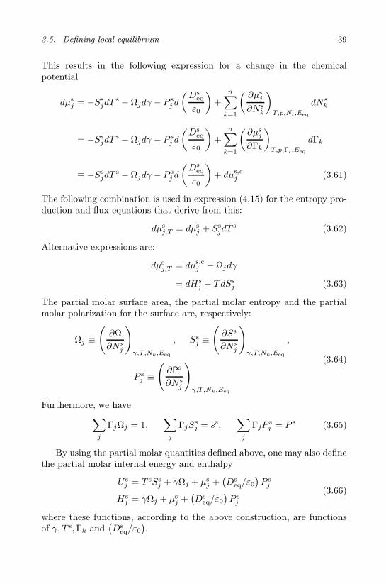
3.5. Defining local equilibrium 39
This results in the following expression for a change in the chemicalpotential
dµsj = −Ss
jdTs − Ωjdγ − P s
j d
(Ds
eq
ε0
)+
n∑
k=1
(∂µs
j
∂N sk
)
T,p,Nl,Eeq
dN sk
= −SsjdT
s − Ωjdγ − P sj d
(Ds
eq
ε0
)+
n∑
k=1
(∂µs
j
∂Γk
)
T,p,Γl,Eeq
dΓk
≡ −SsjdT
s − Ωjdγ − P sj d
(Ds
eq
ε0
)+ dµs,c
j (3.61)
The following combination is used in expression (4.15) for the entropy pro-duction and flux equations that derive from this:
dµsj,T = dµs
j + SsjdT
s (3.62)
Alternative expressions are:
dµsj,T = dµs,c
j − Ωjdγ
= dHsj − TdSs
j (3.63)
The partial molar surface area, the partial molar entropy and the partialmolar polarization for the surface are, respectively:
Ωj ≡(∂Ω
∂N sj
)
γ,T,Nk,Eeq
, Ssj ≡
(∂Ss
∂N sj
)
γ,T,Nk,Eeq
,
P sj ≡
(∂P
s
∂N sj
)
γ,T,Nk,Eeq
(3.64)
Furthermore, we have∑
j
ΓjΩj = 1,∑
j
ΓjSsj = ss,
∑
j
ΓjPsj = P s (3.65)
By using the partial molar quantities defined above, one may also definethe partial molar internal energy and enthalpy
U sj = T sSs
j + γΩj + µsj +
(Ds
eq/ε0)P s
j
Hsj = γΩj + µs
j +(Ds
eq/ε0)P s
j
(3.66)
where these functions, according to the above construction, are functionsof γ, T s,Γk and
(Ds
eq/ε0).

40 Chapter 3. Thermodynamic Relations for Heterogeneous Systems
Exercise 3.A.1. Find a form of Gibbs–Duhem’s equation for the surfacethat contains dµs
j,T instead of dµsj .
• Solution: If we substitute Eq. (3.62) into Eq. (3.32d), we have
0 = ssdT s + dγ +
n∑
j=1
Γjdµsj,T −
n∑
j=1
ΓjSsjdT
s + P sd(Ds
eq/ε0)
By using∑n
j=1 ΓjSsj = ss, Gibbs–Duhem’s equation for the surface
is reduced to
dγ = −n∑
j=1
Γjdµsj,T − P sd
(Ds
eq/ε0)
3.A.3 Standard states
The internal energy or the various derivatives of this energy, including thepartial molar energies cannot be measured, only energy differences are mea-surable. In order to establish a measuring scale, we introduce the standardstate as a point of reference. The standard state may be chosen freely, anddifferent conventions have been made. Common to all choices is that theycan be derived from each other by well-defined measurements.
The standard state for gases used in the SI system is the state of an idealgas at 1 bar and constant temperature. The temperature is not specifiedin the definition of the standard state. Standard state values are oftentabulated at 298 K, however. The definition of the chemical potential thenrelates any state to the standard state via
∫ µ
µ0
dµ =
∫ p
p0
Vmdp (3.67)
where Vm is the molar volume. For an ideal gas, we obtain:
µid = µ0 +RT lnp
p0(3.68)
where µ0 is the standard chemical potential and p0 = 1 bar. The energy ofa real gas is measured with respect to this standard state, with the fugacityf replacing the pressure p of the gas. The chemical potential is:
µ = µ0 +RT lnf
p0= µ0 +RT ln
φp
p0= µid +RT lnφ (3.69)
where the fugacity coefficient, defined by the ratio φ = f/p, measures thedeviation of the real gas from the ideal state, see Fig. 3.5 and exercise 3.A.2.

3.5. Defining local equilibrium 41
µ0
µ
p 0p
lnRT φ
µ id
Figure 3.5 The chemical potential of an ideal gas (stippled line) and a real gas(whole line). The standard state, µ0, at p0 = 1 bar is shown for the ideal gas.The deviation of the chemical potential of the real gas from the correspondingideal gas value at p is measured by the term RT lnφ.
The chemical potential of ideal and real gases are illustrated in this figure.When µ− µid < 0 and φ < 1, attractive forces are important.
For a liquid solution, we use a liquid state as the standard state. Thenumbers to be compared then become closer to each other. Two choices arecommon; the Raoultian standard state (used for solvents) and the Henrianstandard state (used for solutes). The Raoultian standard state is the stateof a solution which obeys Raoult’s law. In this law, the vapor pressure abovethe solution is proportional to the mole fraction of the solvent (component1):
p1 = x1p∗1 (3.70)
where p∗1 is the vapor pressure above the pure solvent. We assume that thevapor above the solution is an ideal gas. Equation (3.68) then gives:
µ1 = µ0 +RT lnp∗1p0
+RT lnp1
p∗1(3.71)
which can be rearranged into
µ1 = µ∗ +RT lnx1 (3.72)
The Raoultian standard state for the solvent is defined by
µ∗ ≡ µ0 +RT lnp∗1p0
(3.73)

42 Chapter 3. Thermodynamic Relations for Heterogeneous Systems
The Raoultian standard state is thus determined from the standard stateof the ideal gas plus a term that contains the vapor pressure of the solvent.A deviation from the Raoultian state is expressed by
µ1 = µ∗ +RT ln a1 = µ∗ +RT ln y1x1 (3.74)
where y1 is the activity coefficient that measures deviation from ideal be-havior, and a1 is the activity, a1 = p1/p
∗1. The situation with y1 > 0 is
illustrated in Fig. 3.6. Such a value means that there are repulsive forces inthe liquid that enhance the vapor pressure above the liquid more than inthe case of a solvent that follows Raoult’s law. This standard state is usedin Chapter 11 on evaporation and condensation.
The Henrian standard state is defined by a solution with a solute (com-ponent 2) of concentration m0
2 = 1 molal, that obeys Henry’s law:
p2 = K2m02 (3.75)
Here, K2 is Henry’s law’s constant. The standard state is hypotheticalas no solution is known to obey Henry’s law at this concentration. Theconstant K2 is determined by measuring the vapor pressure above dilutesolutions. The state is determined by extrapolation of this line to m0
2 = 1molal (see Fig. 3.6). By following the same procedure as above, we obtainfor the chemical potential of an ideal solution:
µ2 = µ+ +RT lnm2/m02 (3.76)
Henry’s law standard state is:
µ+ = µ0 +RT lnK2
p0(3.77)
This standard state is commonly used also for electrolyte solutions.There are two particles formed in a dilute solution per formula weight ofsalt dissolved, leading in the ideal case to
µ2 = µ+ +RT lnm2,+m2,−/(m0
2
)2(3.78)
or in the non-ideal case to:
µ2 = µ+ +RT ln γ2±,mm2,+m2,−/
(m0
2
)2(3.79)
where γ2± is the mean square activity coefficient of the cation and anion.
This standard state, or the state based on molar concentrations, µ0, in
µ2 = µ0 +RT ln γ2±c2,+c2,−/
(c02)2
(3.80)

3.5. Defining local equilibrium 43
p
*p1
x10 1
m0 1
p
K2
2
2
Figure 3.6 The phase diagram for a solution that follows Raoult’s law (p1 =p∗1x1) when x1 → 1 and Henry’s law (p2 = K2m2) when m2 → 1.
are used with chemical potentials of electrolytes, cf. Chapter 10. The valueof µ0 is found from µ+ by converting molalities into concentrations at thestandard state. The mean square activity coefficient is given by Debije–Hückel’s formula, when the solution is dilute.
The chemical potential of a surface-adsorbed component can be referredto a standard state with (a hypothetical) one molar surface excess concen-tration of the component, or a standard state referred to unit coverage, θ,of the surface:
µsj = µ0,s +RT ln Γj/Γ
0
= µ0,s +RT ln θj (3.81)
The standard state must be connected to properties of the adjacent phase,in a similar way as the ideal gas standard state is connected to the Raoul-tian standard state. The symbol θj = Γj/Γ
0 denotes fractional coverage.Activity coefficients corrections to the ideal formula can be substantial ifthe surface is polarized:
µsj = µ0,s +RT ln θjy
sj (3.82)
where ys is the surface activity coefficient of component j.We did not specify the temperature in these definitions. In fact, any
temperature can be chosen. When one wants to compare standard states

44 Chapter 3. Thermodynamic Relations for Heterogeneous Systems
at different temperatures, one will have to use the general relation whichapplies to any state, including the standard state:
(dµ
dT
)
p
= −S (3.83)
Expressions for activity coefficients in gases and liquids can be found inPerry and Green [114].
Exercise 3.A.2. Express the fugacity coefficient φ of a gas in terms of itsmolar volume. The fugacity coefficient is defined as φ = f/p, the ratio of thegas fugacity over the pressure of an ideal gas at corresponding conditions.
• Solution: Equation (3.49) reduces to
dµ ≡ Vmdp
for a pure isothermal gas. Vm is its molar volume. This equation istrue for all gases whether they are ideal or not. The fugacity of a gasis defined by (see e.g. [97])
dµ = RTd ln f
For densities that are low enough, the gas follows the ideal gas law,pVideal = RT . This will always happen at some pressure p′ whenp→ 0 ∫ µ
µ′
dµ =
∫ p
p′
Vmdp = RT lnf
p′
For an ideal gas, the corresponding expression is∫ p
p′
Videaldp = RT lnp
p′
Subtraction and introduction of p′ = 0 gives
lnf
p= lnφ =
1
RT
∫ p
0
(Vm − Videal) dp
The fugacity coefficient is expressed by measurable quantities in thisformula.

Part A: General Theory
45

This page intentionally left blankThis page intentionally left blank

Chapter 4
The Entropy Production
for a Homogeneous Phase
We derive the entropy production in a volume element in a homogeneousphase for transport of heat, mass, charge and chemical reactions. The en-tropy production determines the conjugate fluxes and forces in the phase.Equivalent forms of the entropy production are given.
The second law of thermodynamics, Eq. (2.14), says that the entropychange of the system plus its surroundings is positive for irreversible pro-cesses and zero for reversible processes. The law gives the direction of aprocess; it does not give its rate. Non-equilibrium thermodynamics as-sumes that the second law remains valid locally, cf. Eq. (1.1). In thischapter, we shall derive the entropy production for a volume element in ahomogeneous phase. In the next chapters, we shall find the correspond-ing expressions for a surface area element and a three phase contact lineelement. In total, we will then be able to describe the rate of changes inheterogeneous systems.
The change of the entropy in a volume element in a homogeneous phaseis given by the flow of entropy in and out of the volume element and by theentropy production inside the volume element:
∂s(x, t)
∂t= − ∂
∂xJs(x, t) + σ(x, t) (4.1)
Here, s(x, t) is the entropy density, Js(x, t) is the entropy flux in the lab-oratory frame of reference and σ(x, t) is the entropy production. As theentropy density and flux depend on both position and time, we use partialderivatives. We consider only one-dimensional transport problems.
Below a more explicit expression for σ will be found by combining
• mass balances
47

48 Chapter 4. The Entropy Production for a Homogeneous Phase
• the first law of thermodynamics
• the local form of the Gibbs equation.
We shall do this and compare the resulting expression for the time rateof change of the entropy density with Eq. (4.1). This will make it pos-sible to identify the entropy flux as well as the entropy production. Weshall find that σ can be written as the product sum of the conjugate fluxesand forces in the system, see Sec. 1.1. In the derivation, we follow refer-ences [20] and [27]. Electroneutral-, polarizable-, non-equilibrium systemswith and without chemical reactions are of interest. These are the sys-tems that we encounter most often in nature, and also in industry. Weshall model transport of heat, mass and charge in systems where reactionsoccur. We recommend using the symbol list for checking of dimensionsin the equations. An introduction to non-equilibrium thermodynamics forhomogeneous systems was given by Kjelstrup, Bedeaux and Johannessen[28, 29].
Consider a volume element, V , which is in local equilibrium in a polar-izable, electroneutral bulk phase. The volume element does not move withrespect to the walls (the laboratory frame of reference), see Fig. 4.1. Allfluxes are with respect to the laboratory frame of reference.
Figure 4.1 A volume element in a bulk phase with transport where j ′ indicatesone of the fluxes.
The volume element has a sufficient number of particles to give a statis-tical basis for thermodynamic calculations. Its state is given by the temper-ature T (x, t), chemical potentials µj(x, t) for all the n neutral components,pressure p(x, t) and the equilibrium electric field Eeq(x, t) = Deq(t)/ε(x, t).We shall take ε constant in the homogeneous phases. Both equilibrium

4.1. Balance equations 49
electric fields are then independent of the position:
Eieq(t) = Deq(t)/εi and Eo
eq(t) = Deq(t)/εo (4.2)
The number of positive particles equals the number of negative particles,but their distribution within the volume element can lead to a polarizationdensity.
4.1 Balance equations
The balance equation for component j is
∂cj(x, t)
∂t= − ∂
∂xJj(x, t) + νjr(x, t) for j = 1, ..., n (4.3)
where Jj(x, t) are the component fluxes in the laboratory frame of reference,all directed along the x-axis. Furthermore, νj is the stoichiometric constantof component j in a chemical reaction, which is positive if j is a productand negative if j is a reactant, and r(x, t) is the reaction rate in the volumeelement. For simplicity, we consider only one reaction. It is easy to addmore reactions [20]. The reaction Gibbs energy is
∆rG(x, t) =
n∑
j=1
νjµj(x, t) (4.4)
In our description of reactions at surfaces, we shall also need the contribu-tion to the reaction Gibbs energy due to the neutral species
∆nG(x, t) ≡∑
j ∈ neutral
νjµj(x, t) (4.5)
where the sum in Eq. (4.5) is only over the neutral components. Thedifference between ∆nG and the usual expression ∆rG, is due to the chem-ical potentials of ions and electrons. We explain why we need ∆nG inSecs. 10.6–10.7.
Exercise 4.1.1. Derive Eq. (4.3) for r = 0 by considering changes in avolume element that is fixed with respect to the walls.
• Solution: The change in the number of moles of a component,Nj(x, t), in a small volume V , is due to the flux of the component inand out of the volume. We have:
dNj(x, t)
dt= −Ω[Jj(x+ dx, t) − Jj(x, t)]

50 Chapter 4. The Entropy Production for a Homogeneous Phase
where Ω is the cross sectional area of the volume orthogonal to theflux direction (the fluxes are flows per unit of area). The area is equalto the volume divided by dx. In the limit of small dx, we have
dNj(x, t)
dt= −V [Jj(x+ dx, t) − Jj(x, t)]
dx= −V ∂Jj(x, t)
∂x
By dividing this equation left and right by the (constant) volume, oneobtains Eq. (4.3).
The conservation equation for charge is
∂z(x, t)
∂t= − ∂
∂xj(x, t) (4.6)
where z(x, t) is the charge density. The systems that we consider, canall be described as electroneutral. It follows that ∂j/∂x = 0, so that theelectric current density, j, is constant. The electric current is due to therelative motion of the charge carriers in the system, like for instance ofelectrons relative to the metal ion lattice. This relative motion is such thatit preserves charge neutrality.
According to the first law of thermodynamics, the change in internalenergy density per unit of time is equal to:
∂u(x, t)
∂t= − ∂
∂xJq(x, t) −
∂φ(x, t)
∂xj + E(x, t)
∂P (x, t)
∂t(4.7)
where Jq(x, t) is the total heat flux in the laboratory frame of reference.The product − [∂φ(x, t)/∂x] j is the electrical work done to the volumeelement. The time derivative of the polarization density is the displacementcurrent, jdispl(x, t) ≡ ∂P (x, t)/∂t. The product E(x, t)jdispl(x, t) gives thework per unit of volume by the displacement current. This is a capacitivecontribution which, for instance, is important when there is an oscillatoryelectric field (see Chapter 21). In the appendix at the end of this chaptera discussion is given of the relation between Eq. (4.7), the first law, thedefinition of the total heat flux, and the relation between ∂φ(x, t)/∂x andE(x, t). An important assumption in the derivation of Eq. (4.7) is that thesystem is in mechanical equilibrium, a condition we shall use throughoutthis book. Contrary to the situation in vacuum, the electric field in amedium is not a conservative field.
The total heat flux across the volume element is given by
Jq(x, t) = J ′q(x, t) +
n∑
j=1
Hj(x, t)Jj(x, t) (4.8)

4.2. The entropy production 51
Figure 4.2 The energy change of a volume element with fluxes of heat andcharge across the boundaries.
It consists of the measurable heat flux, J ′q(x, t), and the partial molar en-
thalpies, Hj(x, t), carried by the neutral component fluxes, Jj(x, t). Themeasurable heat flux is independent of the frame of reference. This is notthe case for the total heat flux. We discuss the frame of reference fur-ther in Secs. 4.2, 4.4, Appendix 4.A, and also in Chapter 12, which dealswith multi-component diffusion. The first law is illustrated in Fig. 4.2.De Groot and Mazur [20] used charged and uncharged components, whichis appropriate for systems that are not electroneutral, and defined a re-duced heat flux in analogy with Eq. (4.8). In the electroneutral systems,which we consider, it is more appropriate to use the smaller number ofuncharged components. The measurable heat flux differs from the reducedheat flux by a contribution proportional to the electric current density, seeAppendix 4.A for a discussion.
4.2 The entropy production
The Gibbs equation in its local form, Eq. (3.26) together with Eq. (3.7),
du = Tds+
n∑
j=1
µjdcj + EeqdP (4.9)
is needed to calculate the entropy production. The time derivative of theentropy density becomes, using Eq. (4.9):
∂s(x, t)
∂t=
1
T (x, t)
∂u(x, t)
∂t−
n∑
j=1
µj(x, t)
T (x, t)
∂cj(x, t)
∂t− Eeq(t)
T (x, t)
∂P (x, t)
∂t
(4.10)

52 Chapter 4. The Entropy Production for a Homogeneous Phase
Partial derivatives are used since the variables are position and timedependent.
Exercise 4.2.1. Derive Eq. (4.1) by considering changes in a volume ele-ment fixed with respect to the walls.
• Solution: The change of entropy is due to the flux in and out of thevolume element plus an increase due to the entropy production:
dS(x, t)
dt= −Ω[Js(x+ dx, t) − Js(x, t)] + V σ(x, t)
where σ(x, t) is the entropy production per unit of volume. The crosssection is equal to the volume divided by dx. We obtain in the limitof small dx
dS(x, t)
dt= −V [Js(x+ dx, t) − Js(x, t)]
dx+ V σ(x, t)
= −V dJs(x, t)
dx+ V σ(x, t)
By dividing this equation left and right by the volume, one obtainsEq. (4.1).
By introducing Eqs. (4.3) and (4.7) into (4.10), using the rule for deriva-tion of products, and solving for ∂s(x, t)/∂t, we obtain as balance equationfor the entropy density:
∂s(x, t)
∂t= − ∂
∂x
1
T (x, t)
Jq(x, t) −
n∑
j=1
µj(x, t)Jj(x, t)
+ Jq(x, t)
(∂
∂x
1
T (x, t)
)+
n∑
j=1
Jj(x, t)
(− ∂
∂x
µj(x, t)
T (x, t)
)
+ j
(− 1
T (x, t)
∂φ(x, t)
∂x
)
+∂P (x, t)
∂t
[E(x, t) − Eeq(x, t)
T (x, t)
]+ r(x, t)
(−∆rG(x, t)
T (x, t)
)
(4.11)

4.2. The entropy production 53
To simplify notation, we usually suppress the (x, t) for all variables. Bycomparing the above equation with Eq. (4.1), we identify the entropy flux
Js =1
T
Jq −n∑
j=1
µjJj
=1
TJ ′
q +
n∑
j=1
SjJj (4.12)
and the entropy production in the system
σ = Jq
(∂
∂x
1
T
)+
n∑
j=1
Jj
(− ∂
∂x
µj
T
)+ j
(− 1
T
∂φ
∂x
)
+∂P
∂t
(E − Eeq
T
)+ r
(−∆rG
T
)(4.13)
Here, Sj is the partial molar entropy of component j. By replacing the totalheat flux, Jq, by the entropy flux, Js, we obtain an alternative expression
σ = Js
(− 1
T
∂T
∂x
)+
n∑
j=1
Jj
(− 1
T
∂µj
∂x
)+ j
(− 1
T
∂φ
∂x
)
+∂P
∂t
(E − Eeq
T
)+ r
(−∆rG
T
)(4.14)
We furthermore replace the total heat flux, Jq, by the often more practicalmeasurable heat flux, J ′
q, using Eq. (4.12). The result is
σ = J ′q
(∂
∂x
1
T
)+
n∑
j=1
Jj
(− 1
T
∂µj,T
∂x
)+ j
(− 1
T
∂φ
∂x
)
+∂P
∂t
(E − Eeq
T
)+ r
(−∆rG
T
)(4.15)
where ∂µj,T /∂x = ∂µj/∂x + Sj∂T/∂x is the derivative of the chemicalpotential keeping the temperature constant, see Appendix 3.A. Finally,when one describes heat and charge transport, it is sometimes convenientto replace the total heat flux by the energy flux Ju, which is defined by (seeChapters 9, 15 and 19)
Ju ≡ Jq + φj = J ′q +
n∑
j=1
HjJj + φj (4.16)

54 Chapter 4. The Entropy Production for a Homogeneous Phase
This gives for the entropy production
σ = Ju
(∂
∂x
1
T
)+
n∑
j=1
Jj
(− ∂
∂x
µj
T
)+ j
(− ∂
∂x
φ
T
)
+∂P
∂t
(E − Eeq
T
)+ r
(−∆rG
T
)(4.17)
The results for σ were derived using only the assumption of local equi-librium, see Sec. 3.5. Local equilibrium does not imply local chemicalequilibrium. Local chemical equilibrium is a special case of local equi-librium [20,68].
The entropy production contains pairs of fluxes and forces. These arethe conjugate fluxes and forces defined in Chapter 1. The conjugate flux-force pairs in Eqs. (4.13), (4.14), (4.15) and (4.17) are different. The dif-ferent sets of pairs are, however, equivalent and describe the same physicalsituation. The problem one wants to describe, dictates the form that ismost convenient. Convenient is a form that describes the system in themost direct way. If, for instance, the system is such that the chemical po-tentials of all components are constant, Eq. (4.14) is convenient becauseall terms containing their gradients are zero. The four alternative expres-sions have been given, as a help to find the appropriate final form. Allforces and fluxes have a direction, except the last pair, and are thus vec-tors. The chemical reaction has a scalar flux and force. We shall discussthe consequences of this for isotropic systems in Sec. 7.6.
Remark 4.1. De Groot and Mazur [20] use fluxes in the barycentric frameof reference. We always use fluxes in the laboratory frame of reference.The entropy production is invariant for this transformation. This can beverified for instance in Eq. (4.15). In this expression the only fluxes thatdepend on the frame of reference are the component fluxes. Subtracting fromthese component fluxes, the molar densities times the barycentric velocity,gives a total change which is zero according to Gibbs–Duhem’s equation. Itfollows that one may replace the component fluxes in the laboratory frame ofreference by those in the barycentric frame of reference. See also Sec. 4.4.2.
The separate products do not only give pure losses of work (compareSecs. 2.4 and 7.5). Their sum does. For instance, the electric power per unitof volume, − (j∂φ/∂x), does not necessarily give only an ohmic contributionto the entropy production, there may also be electric work terms includedin the product, as we shall see in detail in Chapters 9 and 10. Each productcontains normally work terms as well as energy storage terms. It is theircombination which gives the entropy production rate, and the work that is

4.2. The entropy production 55
lost per unit of time, dWlost/dt = T0
∫σdV (see Sec. 2.4). The expressions
(4.13)–(4.15) and (4.17) can thus be used to find the second law efficiencyof a process [29].
De Groot and Mazur [20] used the affinity, A, of the chemical reaction,rather than the reaction Gibbs energy, in Eq. (4.15). According to Kon-depudi and Prigogine [56] (page 111), the reaction Gibbs energy is primarilyused in connection with equilibrium states and reversible processes, whilede Donder’s affinity concept is more general, it relates chemical reactionsto entropy. We dispute that there is a principle difference between the twoconcepts. The affinity is simply equal to minus of the reaction Gibbs en-ergy. We use the reaction Gibbs energy, because chemists are more familiarwith this concept.
Ross and Mazur [115] showed that the contribution to σ from the chem-ical reaction was equal to the product of r and the driving force, −∆rG/T ,also when the reaction rate is a non-linear function of the driving force,provided that the ensemble of particles is nearly Maxwellian. Prigogineshowed that the Gibbs relation was valid for such conditions [110].
Haase [21] defined and used the dissipation function in his monographon “Thermodynamics of Irreversible Processes”. The dissipation function isstill in focus in many books, see e.g. Demirel [116]. In homogeneous sys-tems, Haase defined Ψ = TdSirr/dt, where dSirr/dt is the rate of increaseof the entropy due to processes which occur inside the system. For a con-tinuous system, in which the temperature can vary from point to point, heused the definition Ψ = Tσ, [22] page 83. This last definition is analogousto Raleigh’s dissipation function for hydrodynamic flow. For heterogeneoussystems, which are discussed in this book, neither of the above definitionscan be used. On pages 161-164, Haase considered the case of two phases inthermal contact with each other. After calculating the entropy production,he multiplied it with the temperature of one of the phases. In the result-ing expression, he then needed to linearize in the temperature difference ofthe phases, in order to obtain an expression for Ψ which is linear in thetemperature difference. He contributed thereby to the erroneous idea thata non-equilibrium thermodynamic description should be fully linearized.The entropy production he first derived was perfectly linear in the differ-ence of the inverse temperature. When one uses the entropy productionrather than Ψ, as is systematically done in this book, there is no need tofurther linearize. Instead of multiplying with the temperature of one of thephases, it is appropriate to multiply with the temperature of the environ-ment as is done in exergy analysis to find the lost work. We discussed inSec. 2.4 that this gives the lost work. We strongly advise against using Ψin heterogeneous systems, see Sec. 4.2.1 for further arguments.

56 Chapter 4. The Entropy Production for a Homogeneous Phase
Changing the frame of reference does not change the value or the phys-ical interpretation of σ. The entropy production is an absolute quantity.It is invariant for transformations to other frames of reference, i.e. it is“Galilean invariant”. Possible choices for the frame of reference will bediscussed in Sec. 4.4.
As mentioned above, we are dealing only with one-dimensional transportproblems in this book. That is, we consider only transport normal to thesurface. All densities and fluxes are assumed to be independent of thecoordinates along the surface and the vectorial fluxes are assumed to bedirected normal to the surface. These assumptions can be made because thesystems we consider are isotropic along the surface. A system is isotropicif it is invariant for translation along the surface, for rotation around anormal on the surface, and for reflection with respect to planes normal tothe surface.
Compression is a scalar phenomenon that couples to the reactions inthe bulk phases. This coupling is small, however, since density variationsrelax on a time scale of the size of the system divided by the velocity ofsound. The assumption of mechanical equilibrium, grad p = 0, used toderive Eq. (4.7), is therefore often valid, see [20] for a discussion of themore general case. In the absence of compression, the compressional (bulk)viscosity does not play a role.
Convection and shear flow will disturb chemical reactions and transportof heat and mass, but do not couple to them directly. Convection and/orshear flow can be described by non-equilibrium thermodynamics, see e.g.[30, 31], but will not be considered in this book.
4.2.1 Why one should not use the dissipation function
Consider three thermal reservoirs with internal energies Ua, Ub, Uc andtemperatures Ta, Tb, Tc. The reservoirs are in thermal contact and therates of change of these internal energies are
dUa
dt= −Jab
q − Jacq ,
dUb
dt= −Jba
q − Jbcq ,
dUc
dt= −Jca
q − Jcbq
where J ijq = −Jji
q is the heat flux from reservoir i to reservoir j. The totalinternal energy U = Ua + Ub + Uc is conserved
dU
dt=dUa
dt+dUb
dt+dUc
dt= 0
The rate of change of the entropy of the reservoirs is given by the Gibbsrelation
dSi
dt=
1
Ti
dUi
dtfor i = a, b, c

4.2. The entropy production 57
The total entropy production is
dSirr
dt=dSa
dt+dSb
dt+dSc
dt=
1
Ta
dUa
dt+
1
Tb
dUb
dt+
1
Tc
dUc
dt
= Jabq
(1
Tb− 1
Ta
)+ Jac
q
(1
Tc− 1
Ta
)+ Jbc
q
(1
Tc− 1
Tb
)
For the total dissipation function we obtain
Ψ = TadSa
dt+ Tb
dSb
dt+ Tc
dSc
dt=dUa
dt+dUb
dt+dUc
dt= 0
Linear force-flux relations follow in a straight forward manner from dSirr/dt.The total dissipation function is zero, however, and does not give any force-flux pairs. Haase tried to save himself from this dilemma by multiplying theentropy productions of all reservoirs with the same temperature. Haase [22](pages 161-164) chose the temperature of one of the reservoirs in a case withtwo reservoirs. This procedure is unsystematic as the answer depends onthe reservoir chosen.
Also, exergy analysis (cf. Sec. 2.4) tells that the proper temperaturefor multiplication with the entropy production is the temperature of theenvironment. Correct linear force-flux relations are therefore obtained fromthe entropy production, or equivalently from the lost exergy, but not fromthe dissipation function.
4.2.2 States with minimum entropy production
When a system is close to global equilibrium, one may linearize the equa-tions that describe the time evolution of the system. All the transport co-efficients in Eq. (1.2) are then constant. Prigogine showed that stationarystates of discontinuous systems, maintained for instance by a temperaturedifference, have a minimum entropy production [15]. This is sometimescalled the Prigogine principle. For stationary states far from global equi-librium, the transport coefficients are no longer constant across the wholesystem, and the stationary state has no longer a minimum entropy produc-tion compared to non-stationary states [117,118].
In the design of industrial systems, it is fruitful to ask a different ques-tion. We can ask for the path that a system must follow to obtain minimumentropy production [119]. This question leads to an optimization problemthat is constrained by the performance, for instance by the compositionof the chemicals that are produced. The transport coefficients of the sys-tem are then considered as given. The nature of systems with minimumtotal entropy production dSirr/dt has been studied extensively since 1982

58 Chapter 4. The Entropy Production for a Homogeneous Phase
by Bejan and coworkers, see [84, 85] (mostly mechanical systems) and byKjelstrup and coworkers since 1995, see [29] (mostly chemical systems).
Johannessen and Kjelstrup [91] found that much of the path of an op-timal chemical reactor was characterised by constant local entropy produc-tion, provided that the system had enough degrees of freedom to find thispath. This was called the highway hypothesis. In all cases, the entropyproduction and not the dissipation function, was used as proper objectivefunction. Bejan [85] (page 227) showed that the state of minimum entropyproduction was equal to the state of maximum power, contrary to otherclaims [120], see also [29].
4.3 Examples
The exercises below illustrate how single contributions arise in the entropyproduction. Some exercises are meant to illustrate the theory. The re-maining give numerical and physical insight. Transport of heat at lowtemperatures and chemical reactions give relatively large losses of work.
Exercise 4.3.1. Consider the special case that only component number jis transported. The densities of the other components, the internal energy,the molar volume and the polarization densities are all constant. Show thatthe entropy production is given by
σ = −Jj∂
∂x
(µj
T
)
• Solution: In this case Eq. (4.10) reduces to
T∂s
∂t+ µj
∂cj∂t
= 0
The rate of change of the entropy is therefore given by
∂s
∂t= −µj
T
∂cj∂t
Now we use Eq. (4.3) for component j and obtain
∂s
∂t=µj
T
∂
∂xJj =
∂
∂x
(µi
TJj
)− Jj
∂
∂x
µj
T
Comparing this equation with Eq. (4.1) we may identify the entropyflux and the entropy production as
Js = −µj
TJj and σ = −Jj
∂
∂x
(µj
T
)

4.3. Examples 59
Exercise 4.3.2. Consider the case that only heat is transported. The molardensities, the molar volume and the polarization densities are all constant.Show that the entropy production is given by
σ = J ′q
∂
∂x
(1
T
)
• Solution: In this case Eq. (4.10) reduces to
∂u
∂t= T
∂s
∂t
The rate of change of the entropy is therefore given by
∂s
∂t=
1
T
∂u
∂t
Eq. (4.7) reduces to∂u
∂t= − ∂
∂xJ ′
q
By substituting this into the equation above, we obtain
∂s
∂t= − 1
T
∂
∂xJ ′
q = − ∂
∂x
1
TJ ′
q + J ′q
∂
∂x
1
T
By comparing this equation with Eq. (4.1), we can identify the en-tropy flux and the entropy production as
Js =1
TJ ′
q and σ = J ′q
∂
∂x
(1
T
)
Exercise 4.3.3. Find the entropy production due to the heat flux througha sidewalk pavement by a hot plate placed d = 8 cm under the top of thepavement. The plate has a temperature of 343 K, and the surface is incontact with melting ice (273 K). The Fourier type thermal conductivity ofthe pavement is 0.7 W/m K.
• Solution: Fourier’s law for heat conduction is J ′q = −λ(dT/dx). The
entropy production per m2 is rather large:
1
d
∫ d
0
σdx =1
d
∫ d
0
J ′q
∂
∂x
(1
T
)dx = −λ∆T
d2
(1
T2− 1
T1
)
= −0.7(−70)
(0.08)2
(1
273− 1
343
)= 5.7 W/K m3
It is typical for heat conduction around room temperature that lossesare large.

60 Chapter 4. The Entropy Production for a Homogeneous Phase
Exercise 4.3.4. Consider a system with two components (n = 2), havingdT = 0, dp = 0, and dEeq = 0. Show, using Gibbs–Duhem’s equation, thatone may reduce the description in terms of two components to one withonly one component.
• Solution: Gibbs–Duhem, Eq. (3.27), gives:
c1dµ1 + c2dµ2 = 0
The entropy production of Eq. (4.13) reduces for these conditions to:
σ =
(J1
c1− J2
c2
)[−c1T
∂µ1
∂x
]
The equation contains only one independent force. Energy is lost byinterdiffusion of the two components. We can also write this entropyproduction by
σ = v12
[−c1T
∂µ1
∂x
]
with v12 ≡ J1/c1−J2/c2. This is the velocity of component 1 relativeto the velocity of component 2. Note that v12 is independent of theframe of reference.
Exercise 4.3.5. We are interested in the filtering of water (w) across asandy layer of 1 m at 293 K. Evaluate the entropy production for a waterflux of 10−6 kg/m2s. The density of the sand at 293 K is ρ =1940 kg/m3
[121]. The volume of water per unit of mass is Vw = 103 m3/kg.
• Solution: The only contribution to the chemical potential gradientis from the pressure (dµc
w = 0), so dµw,T = Vwdp. The pressure onwater at a distance x from the surface is given by the weight of thesand, p = ρgx. This gives dµw,T /dx = Vwρg, and
σ = −Jw1
TVwρg = 6.5 × 10⁻⁸ W/ K m3
This value is considerably smaller than the value for transport of heatacross a pavement (see exercise 4.3.3).
Exercise 4.3.6. Give the details of the derivation of Eq. (4.15) fromEq. (4.13).

4.3. Examples 61
• Solution: We first rewrite the negative force as
∂
∂x
(µj
T
)=
∂
∂x
(µj
T
)
T+
∂
∂T
(µj
T
) ∂T∂x
=1
T
∂
∂xµj,T +
(1
T
∂µj
∂T− µj
T 2
)∂T
∂x
=1
T
∂
∂xµj,T − 1
T 2(TSj + µj)
∂T
∂x=
1
T
∂
∂xµj,T +Hj
∂
∂x
1
T
By substituting this result into Eq. (4.13), we obtain
σ =
Jq −n∑
j=1
HjJj
∂
∂x
(1
T
)+
n∑
j=1
Jj
(− 1
T
∂
∂xµj,T
)
+ j
(− 1
T
∂φ
∂x
)+∂P
∂t
[− 1
T
∂(φ− φeq)
∂x
]
By using Jq = J ′q +
∑nj=1HjJj , Eq. (4.15) follows.
Exercise 4.3.7. Derive the entropy production for an isothermal two-component system that does not transport charge. The solvent is the frameof reference for the fluxes.
• Solution: In an isothermal system, ∂(1/T )/∂x = 0. Furthermore,there is no charge transport so that j = 0. Finally, the solvent is theframe of reference, so Jsolvent = 0. There remains only one force-fluxpair, namely for transport of solute. Using Eq. (4.15), we then find
σ = −J
T
∂µT
∂x
for the entropy production. Using that σ ≥ 0 it follows that the solutewill move from a higher to a lower value of its chemical potential.
Exercise 4.3.8. What is the entropy production for systems that are de-scribed by Eqs. (2.1), (2.2) and (2.3)?
• Solution: Substitution of these equations into Eq. (4.15), setting thereaction rate and the displacement current zero, yields
σ =λ
T 2
(∂T
∂x
)2
+D
T
∂µT
∂x
∂c
∂x+κ
T
(∂φ
∂x
)2
=λ
T 2
(∂T
∂x
)2
+D
T
∂µT
∂c
(∂c
∂x
)2
+κ
T
(∂φ
∂x
)2
≡ σT + σµ + σφ

62 Chapter 4. The Entropy Production for a Homogeneous Phase
Typical values in an electrolyte are: λ = 2 J/msK, T = 300 K,dT/dx = 100 K/m, D = 10−9 m2/s, ∂µT /∂c = RT/c, c = 100kmol/m3, dc/dx = 10−5 mol/m4, κ = 400 Si/m, dφ/dx = 10−2
V/m. The resulting entropy productions are: σT = 0.2 J/Ksm3, σµ =10−13 J/Ksm3 and σφ = 10−4 J/Ksm3. Heat conduction thereforeclearly gives the largest contribution to the entropy production inelectrolytes.
Exercise 4.3.9. What is the first law efficiency ηI for a Carnot machine?Compare this efficiency with the expression for the entropy production of asystem that transports heat from a hot reservoir to the surroundings.
• Solution: The Carnot machine transforms heat into work in a re-versible way. The efficiency is defined as the work output divided bythe heat input [97,122]. This efficiency is (Th−Tc)/Th, where Th andTc are the temperatures of the hot and the cold reservoir, respectively.If we do not use the heat to produce work, but simply bring the hotand cold reservoirs in thermal contact with one another, one gets aheat flow from the hot to the cold reservoir. The entropy productionfor the whole (one-dimensional) path, with a cross section Ω is:
dSirr
dt= Ω
∫σ(x)dx = Ω
∫J ′
q(x)∂
∂x
(1
T (x)
)dx
As there is no other transport of thermal energy, the heat flux isconstant and equal to dQ/dt for a unit area. This results in
dSirr
dt= J ′
qΩ
∫∂
∂x
(1
T (x)
)dx = J ′
qΩ
∫ Tc
Th
∂
∂T
(1
T
)dT
= ΩdQ
dt
(1
Tc− 1
Th
)= Ω
dQ
dt
(Th − Tc
ThTc
)= Ω
ηI
Tc
dQ
dt
The work lost per unit of time, TcdSirr/dt, is identical to the work thatcan be obtained by a Carnot cycle, ΩηI(dQ/dt), per unit of time. Thiscan be used as a derivation of the first law efficiency of the Carnotmachine. This machine is reversible and has as a consequence no lostwork. This implies that the work done by the Carnot machine mustbe equal to ΩηI(dQ/dt).
Exercise 4.3.10. Consider the reaction:
B + C D
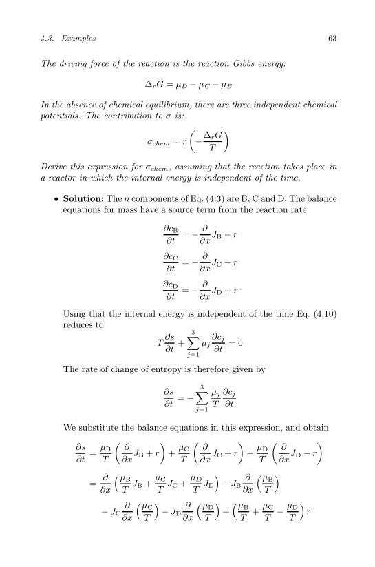
4.3. Examples 63
The driving force of the reaction is the reaction Gibbs energy:
∆rG = µD − µC − µB
In the absence of chemical equilibrium, there are three independent chemicalpotentials. The contribution to σ is:
σchem = r
(−∆rG
T
)
Derive this expression for σchem, assuming that the reaction takes place ina reactor in which the internal energy is independent of the time.
• Solution: The n components of Eq. (4.3) are B, C and D. The balanceequations for mass have a source term from the reaction rate:
∂cB∂t
= − ∂
∂xJB − r
∂cC∂t
= − ∂
∂xJC − r
∂cD∂t
= − ∂
∂xJD + r
Using that the internal energy is independent of the time Eq. (4.10)reduces to
T∂s
∂t+
3∑
j=1
µj∂cj∂t
= 0
The rate of change of entropy is therefore given by
∂s
∂t= −
3∑
j=1
µj
T
∂cj∂t
We substitute the balance equations in this expression, and obtain
∂s
∂t=µB
T
(∂
∂xJB + r
)+µC
T
(∂
∂xJC + r
)+µD
T
(∂
∂xJD − r
)
=∂
∂x
(µB
TJB +
µC
TJC +
µD
TJD
)− JB
∂
∂x
(µB
T
)
− JC∂
∂x
(µC
T
)− JD
∂
∂x
(µD
T
)+(µB
T+µC
T− µD
T
)r
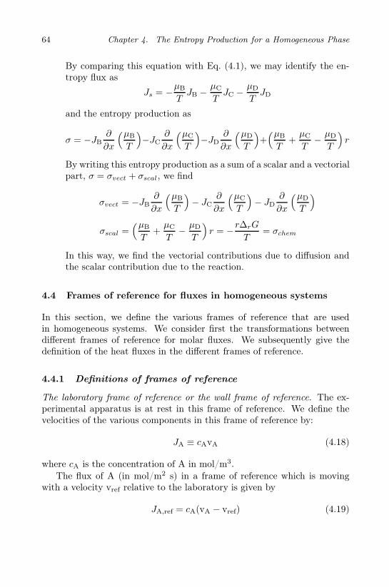
64 Chapter 4. The Entropy Production for a Homogeneous Phase
By comparing this equation with Eq. (4.1), we may identify the en-tropy flux as
Js = −µB
TJB − µC
TJC − µD
TJD
and the entropy production as
σ = −JB∂
∂x
(µB
T
)−JC
∂
∂x
(µC
T
)−JD
∂
∂x
(µD
T
)+(µB
T+µC
T− µD
T
)r
By writing this entropy production as a sum of a scalar and a vectorialpart, σ = σvect + σscal, we find
σvect = −JB∂
∂x
(µB
T
)− JC
∂
∂x
(µC
T
)− JD
∂
∂x
(µD
T
)
σscal =(µB
T+µC
T− µD
T
)r = −r∆rG
T= σchem
In this way, we find the vectorial contributions due to diffusion andthe scalar contribution due to the reaction.
4.4 Frames of reference for fluxes in homogeneous systems
In this section, we define the various frames of reference that are usedin homogeneous systems. We consider first the transformations betweendifferent frames of reference for molar fluxes. We subsequently give thedefinition of the heat fluxes in the different frames of reference.
4.4.1 Definitions of frames of reference
The laboratory frame of reference or the wall frame of reference. The ex-perimental apparatus is at rest in this frame of reference. We define thevelocities of the various components in this frame of reference by:
JA ≡ cAvA (4.18)
where cA is the concentration of A in mol/m3.The flux of A (in mol/m2 s) in a frame of reference which is moving
with a velocity vref relative to the laboratory is given by
JA,ref = cA(vA − vref) (4.19)

4.4. Frames of reference for fluxes in homogeneous systems 65
The solvent frame of reference. This frame of the reference is typicalwhen there is an excess of one component, the solvent. For transport of Arelative to the solvent one has:
JA,solv = cA (vA − vsolv) and vref = vsolv (4.20)
The frame of reference moves with the velocity of the solvent, vsolv.The average molar frame of reference. In a multicomponent mixture,
there is no excess of one component, and we use the average molar velocity:
vmolar ≡1
c
∑
j
cjvj =∑
j
xjvj (4.21)
Here, xj = cj/c is the mole fraction of component j. This gives as fluxof A:
JA,molar ≡ cA (vA − vmolar) (4.22)
The average volume frame of reference is used when transport occursin a closed volume. The average volume velocity is
vvol ≡∑
j
cjVjvj (4.23)
where Vj is the molar volume of component j. The flux of A becomes
JA,vol ≡ cA (vA − vvol) (4.24)
The barycentric (average center of mass) frame of reference. This frameof reference is used in the Navier–Stokes equation. The average mass ve-locity is
vbar ≡1
ρ
∑
j
ρjvj (4.25)
where ρ is the mass density of the fluid, and ρj are the partial mass densities.The flux of A in mol/m2s in the barycentric frame of reference is therefore
JA,bar ≡ cA (vA − vbar) (4.26)
In the barycentric frame of reference, the dimension of the component fluxesused is normally kg/m2s [20]. The flux in kg/m2s is found by multiplicationwith MA, the molar mass, MAJA,bar ≡ ρA (vA − v). This is the diffusionflux of component A. The sum of these diffusion fluxes (in kg/m2s) overall neutral components is equal to zero.

66 Chapter 4. The Entropy Production for a Homogeneous Phase
Remark 4.2. In our analysis we only consider electroneutral systems. Thesum in Eq. (4.25) is therefore over neutral components. In charged systems,like those considered by de Groot and Mazur [20], the sum is over chargedand uncharged components. For electroneutral systems, this results in anaverage mass velocity which differs from the one that we use by a termproportional to the electric current density. We refer to the Appendix atthe end of this chapter for an example.
In this book, we consider heterogeneous systems. As will be explainedin the next two sections, the excess entropy production of a surface and athree phase contact line should be calculated in a frame of reference whichmoves along with the surface or the contact line. We refer to these asthe surface frame of reference and the contact line frame of reference. Forpractical reasons, the same frame of reference is usually taken for fluxes inthe adjacent homogeneous phases. As will be explained in Chapter 12, formulti-component diffusion, one can use Gibbs–Duhem’s equation to obtainflux-force relations, which are independent of the frame of reference. Foreach example considered in this book, we shall indicate which frame ofreference is used and why.
4.4.2 Transformations between the frames of reference
In an electroneutral system, the electric current density j is independent ofthe frame of reference. The measurable heat flux, J ′
q, is also independent ofthe frame of reference. The total heat flux, the mass fluxes and the entropyflux depend on the frame of reference. In the laboratory or the wall frameof reference, we denote these fluxes by Jq, Jk and Js. In any other frameof reference they become:
Jq,ref = Jq + vref
n∑
j=1
cjHj = Jq + vrefH
Jk,ref = Jk + vrefck
Js,ref = Js + vref
n∑
j=1
cjSj = Jq + vrefS
(4.27)
All frames of reference defined above can be used for vref.We consider in this book systems that are in mechanical equilibrium.
The hydrostatic pressure is then constant and there are no shear forces.

4.4. Frames of reference for fluxes in homogeneous systems 67
The Gibbs–Duhem’s equation for constant pressure is:
sdT +
n∑
j=1
cjdµj = 0 (4.28)
By substituting Jq,ref, Jj,ref and Js,ref into Eqs. (4.13)–(4.15), we find, usingGibbs-Duhem’s equation, that the term proportional to vref gives a zerocontribution to the entropy production. This result is Prigogine’s theorem[20].
Gibbs–Duhem’s equation gives a possibility to eliminate a thermody-namic force. Galilean invariance gives a possibility to eliminate a massflux. One property is a consequence of the other, as we have seen above.De Groot and Mazur [20] used systematically the barycentric frame of ref-erence, because they also treated hydrodynamic phenomena. In this frameof reference, the sum of the mass (diffusion) fluxes is zero (see above). Thetotal heat flux Jq,bar equals the heat flux Jq used by de Groot and Mazur.
4.A Appendix: The first law and the heat flux
The purpose of this appendix is to show how the description of de Grootand Mazur is compatible with the one used in this book. The analysis usesas starting point Chapter XIV in de Groot and Mazur [20]. We restrictourselves to the case that the magnetic field and the magnetization arezero. The system is also electroneutral. As a final simplification we shallassume the system to be in mechanical equilibrium. The last simplificationleads to a form of the first law appropriate for the systems described in thisbook, Eq. (4.7). Vectors shall be indicated by bold letters in this appendix,meaning that they have an arbitrary direction, rather than being restrictedto the x-direction as in most of the book.
For a system in which there are no magnetic field or magnetization, theMaxwell equations (in SI units) can be written as
ε0 div E = − divP
rotE = 0
ε0∂
∂tE = j − ∂
∂tP
(4.29)
where ε0 is the dielectric constant of vacuum, E the electric field, j theelectric current density and P the polarization density (in C/m2).

68 Chapter 4. The Entropy Production for a Homogeneous Phase
For the molar density of component j, we have the following conserva-tion equation
∂cj∂t
= − div (cjvj) = − divJj (4.30)
where vj and Jj are the velocity and the molar flux of component j. Thepotential energy density satisfies
∂
∂t
∑
j
cjψj = − div
∑
j
ψjJj
+∑
j
Jj ·Fj (4.31)
where ψj is the potential energy per mole of component j, and Fj = − gradψj is the external force acting on component j, due to this potential. Forthe energy of the electric field, we have
∂
∂t
(1
2ε0E
2
)= ε0E· ∂
∂tE = − E·
(j+
∂
∂tP
)(4.32)
where we used the third Maxwell equation, Eq. (4.29c). Adding the lasttwo equations results in
∂
∂t
∑
j
cjψj +1
2ε0E
2
= − div∑
j
ψjJj
− E ·(j+
∂
∂tP
)−∑
j
Fj · Jj (4.33)
Integrating this relation over a time independent volume V, gives
d
dt
∫
V
∑
j
cjψj +1
2ε0E
2
dr = −
∫
O
∑
j
ψjJj,ndO
−∫
V
E ·
(j+
∂
∂tP
)+∑
j
Fj · Jj
dr
(4.34)
where O is the surface of the volume, dr ≡ dxdydz is the volume element,and subscript n indicates the component of a vector normal to the surface.This expression shows that the sum of the potential and electromagneticenergies changes due to two terms. The first gives the potential energylosses from mass flow through the surface. The second term describes the

4.4. Frames of reference for fluxes in homogeneous systems 69
energy conversion inside the volume. The above expression for the time rateof change of the sum of the potential and electric field energy follows fromconservation of mass and the Maxwell equations. No energy conservationhas yet been used.
The total energy density per unit of volume, e, also contains the internalenergy density per unit of volume u. We therefore have
e = u+∑
j
cjψj +1
2ε0E
2 (4.35)
In the description in this book we use fluxes in the laboratory frame of refer-ence. We do not use fluxes in the barycentric frame of reference. Therefore,we do not subtract kinetic energy from e in order to get u. As the totalenergy is conserved, one has
∂e
∂t= − div Je (4.36)
where Je is the total energy flux. In order to proceed, we need an expressionfor the total heat flux.
Consider the example of an electrolyte solution of NaCl. The salt iscompletely dissociated into ions and due to the reactions at the electrodesurfaces, the chloride ion carries the charge. The system is electroneutraland as a consequence
cCl−(r, t) = cNa+(r, t) = cNaCl(r, t) (4.37)
The time rate of change of these concentrations is given by
∂cNaCl
∂t= − div JCl− = − div JNa+ (4.38)
The electric current density is
j = F (JNa+ − JCl−) (4.39)
where F is faraday’s constant. Together with Eq. (4.38) it follows that
div j = 0 (4.40)
This also follows from the electroneutrality condition. Given that thesodium ions only move as part of the salt, it follows that the ion fluxesare given by
JNa+ = JNaCl and JCl− = JNaCl −j
F(4.41)
in terms of the salt flux and the electric current density.

70 Chapter 4. The Entropy Production for a Homogeneous Phase
The energy flux in the laboratory frame of reference consists of potentialenergy which flows along with the molar fluxes, energy of the charge carrierwhich is carried by the electric current density and of the total heat flux inthe laboratory frame of reference
Je =∑
j
ψjJj − µCl−j
F+ Jq (4.42)
In order to see how the first law of thermodynamics reads for the internalenergy, we subtract Eq. (4.33) from Eq. (4.36) and use Eqs. (4.35) and(4.42). This results in
∂u
∂t= − divJq +
(E + grad
µCl−
F
)· j + E· ∂
∂tP +
∑
j
Fj · Jj (4.43)
The electric field is equal to minus the gradient of the Maxwell potential
E(r, t) = − gradψ(r, t) (4.44)
The φ-potential we use in Eq. (4.7) is equal to
φ(r, t) ≡ ψ(r, t) − µCl−(r, t)
F(4.45)
This is equal to minus the electrochemical potential of chloride ions dividedby the charge of a mole of chloride ions. Electrochemical potentials werefirst defined by Guggenheim [63, 95]. Using this potential, Eq. (4.43) canbe written as
∂u
∂t= − divJq − gradφ · j + E· ∂
∂tP +
∑
j
Fj · Jj (4.46)
Integrating this relation over a time independent volume V gives
d
dt
∫
V
udr = −∫
O
Jq,ndO
+
∫
V
− gradφ · j + E · ∂
∂tP +
∑
j
Fj · Jj
dr (4.47)
This is a more familiar form of the first law. The internal energy changesdue to a total heat flux through the surface. The volume integral containswork added to the system. The first term is the electric work added, and

4.4. Frames of reference for fluxes in homogeneous systems 71
the second is the work done by the displacement current. In the absenceof external forces, and with one-dimensional flow conditions, Eq. (4.46)reduces to Eq. (4.7). Though we restricted the analysis to an example, theresult is generally valid. We also refer to Sec.10.6 in this context.
To further compare our analysis with that of de Groot and Mazur, weverify that the barycentric velocity in a description using charged compo-nents differs from that in a description using uncharged components, i.e.when the system is electroneutral. We do this for the example above, NaClin water. The barycentric velocity in the description using charged compo-nents is
vcharged =MNa+JNa+ +MCl−JCl− +MH2OJH2O
MNa+cNa+ +MCl−cCl− +MH2OcH2O
=MNa+JNaCl +MCl−
(JNaCl − j
F
)+MH2OJH2O
MNa+cNa+ +MCl−cCl− +MH2OcH2O
=MNaClJNaCl −MCl−
j
F +MH2OJH2O
MNaClcNaCl +MH2OcH2O
=MNaClJNaCl +MH2OJH2O
MNaClcNaCl +MH2OcH2O− MCl−
MNaClcNaCl +MH2OcH2O
j
F
= vuncharged − MCl−
MNaClcNaCl +MH2OcH2O
j
F(4.48)
The electric current does not only carry charge, but also mass. This gives adifference between the barycentric velocities calculated using only neutralcomponents and the one calculated using charged components. As we donot use fluxes in the barycentric frame of reference in this book, this doesnot lead to any complications in our analysis.
Also the measurable heat flux is different in the two descriptions. Wehave
J′chargedq = Jq − hNa+JNa+ − hCl−JCl− − hH2OJH2O
= Jq − hNaClJNaCl − hH2OJH2O + hCl−j
F
= J′unchargedq + hCl−
j
F(4.49)
The difference is the enthalpy of the charge carrier carried along by theelectric current. We note that Jq and Js, both in the laboratory frame of

72 Chapter 4. The Entropy Production for a Homogeneous Phase
reference, are the same whether one uses charged or uncharged components.In view of the fact that hCl− is not measurable it is appropriate to callJ′uncharged
q as measurable. De Groot and Mazur named J′chargedq the reduced
heat flux.Finally, we show, again for the same example, that both descriptions
give the same entropy production. To simplify the system further we ne-glect the contribution due to the displacement current. This is the caseconsidered by de Groot and Mazur [20] in Chapter XIII. On page 344 inEq. (40) they give the entropy production in a system with no magneticfield,
Tσ = −Js · gradT − JNa+ · (gradµNa+ − FE) − JCl− · (gradµCl− + FE)
− JH2O · gradµH2O (4.50)
In the analysis of de Groot and Mazur all fluxes are in the barycentric frameof reference. For a system in mechanical equilibrium, one may replace all ofthem by their value in the laboratory frame of reference. The difference isa term which is zero, according to Gibbs–Duhem’s equation. The fact thatthe expression is correct in an arbitrary frame of reference if the system is inmechanical equilibrium, is called Prigogine’s theorem [15]. Using Eq. (4.41)for the ion fluxes, we obtain
Tσ = −Js · gradT − JNaCl · gradµNa+µCl−
− JH2O · gradµH2O +j
F· (gradµCl− + FE)
= −Js · gradT − JNaCl · gradµNaCl − JH2O · gradµH2O − j · gradφ(4.51)
This is the expression we gave in Eq. (4.14) for the case that there is nopolarization and no chemical reaction.

Chapter 5
The Excess Entropy Production for
the Surface
We derive the entropy production for a surface area element. The en-tropy production determines the conjugate fluxes and forces. Equivalentforms of the entropy production are given. The forms contain finite differ-ences of intensive variables into, out of and across the surface as drivingforces.
We are interested in the energy conversion that takes place at surfaces.The surface has a thickness that is small compared to the thickness of theadjacent homogeneous phases. The thermodynamic properties of the sur-face can then be defined using Gibbs method, as surface excess densitiesof mass, entropy, energy and polarization, see Chapter 3. Following Be-deaux, Albano and Mazur [2,3] and Bertrand and Prud’homme [59,60], weshall now make the crucial assumption that surface excess densities can bedefined, and thermodynamic relations remain valid, also when the systemis out of equilibrium. That is, we assume local equilibrium in the surface,cf. Sec. 3.5.
We are seeking a systematic way to set up equations of transport forheat, mass and charge into, out of and across such autonomous surfaces.Such equations will allow us to model, for instance, electrochemical reac-tions or phase transitions, phenomena that need a surface to occur. Inthe homogeneous phases, the variables are continuous. In contrast, atthe surface, we have a discrete situation with fluxes directed into and outof the surface. The surface may act as a source of heat or energy, andfluxes may be discontinuous. The situation is typical for phase transitions,distillation, heterogeneous catalysis, electrochemical reactions to name afew [38, 61, 123–125]. We shall not consider transport along the surface.For this we refer to [2, 3].
73

74 Chapter 5. The Excess Entropy Production for the Surface
We stated in Chapter 4 that the second law must apply to any volumeelement of a homogeneous phase. This statement is now extended to thesurface area element, with the entropy balance
d
dtss(t) − J i,o
s (t) + Jo,is (t) = σs(t) ≥ 0 (5.1)
Here, dss(t)/dt is the rate of change of the excess entropy density per unitof surface area. This is equal to the entropy flux into the surface, minus theentropy flux out of the surface, plus the excess entropy production, σs(t).The asymptotic value of the entropy flux in phase i, J i,o
s (t), is directed intothe surface, while the entropy flux in phase o, Jo,i
s (t), is directed out ofthe surface, see Fig. 5.1. According to the second law, this excess entropyproduction is positive for the surface.
We use straight derivatives, because the excess surface entropy dependsonly on the time, not on the position. The first roman superscript givesthe phase; i, s or o in this case. The second superscript, o or i, indicatesthe phase across the surface. The combination i,o means therefore thevalue in phase i as close as possible to the o-phase at the interface. Thenotation is also illustrated in Fig. 5.5. Balance equations of the form (5.1)can be derived from a continuous description, as was done by Albano etal. [106,126], or using non-equilibrium statistical mechanics as was done byRonis et al. [127, 128].
A short overview of the objectives and the methods used was given byBedeaux and Kjelstrup [61].
5.1 The discrete nature of the surface
On a macroscopic scale the surface is two-dimensional. In Fig. 5.1, we givean enlarged picture of the surface using a nanometer scale. On this scalethe surface area element appears as a volume element with thickness δ. Onthe nanometer scale the fluxes in the homogeneous phases are in very goodapproximation constant, and we may therefore define the asymptotic valuesof these fluxes by:
J i,os (t) ≡ J i
s(a, t) and Jo,is (t) ≡ Jo
s (b, t) (5.2)
where a refers to the start, and b refers to the end of the surface, see Fig. 3.2.We shall find explicit expressions for σs(t), along the same lines as for
σ(x, t) of the homogeneous phase in Chapter 4 by combining:
• mass balances
• the first law of thermodynamics

5.2. The behavior of the electric fields and potential through the surface 75
J Js sσ
δ
i o
nmx /
ss
sds / dt
a b
Figure 5.1 The change of the excess surface entropy density due to entropyfluxes in and out of the surface and entropy production in the surface. Thesurface thickness, δ = b−a, is small compared to the thickness of the adjacentphases.
• the local form of the Gibbs equation.
We shall see that also σs(t) can be written as the product sum of thermo-dynamic fluxes and forces in the system. These are the conjugate fluxesand forces for the surface. The fluxes and forces will be used in subsequentchapters to describe transports across and into the surface in various hetero-geneous systems. Again, we choose the positive direction of transport fromleft to right. The fluxes in this chapter are always in the surface frame ofreference, which is the frame of reference in which the surface is at rest. Inother frames of reference, see Sec. 4.4, the balance equations for the excessdensities, like Eq. (5.1) for the excess entropy density, have to be modifiedwith terms linear in the velocity of the surface [2–4]. We recommend to usethe symbol list for a check of the dimensions in the equations.
5.2 The behavior of the electric fields and potential through
the surface
The excess entropy production of the surface can contain electric drivingforces. We define here the excess electric field Es and excess polarizationP s. The normal component of the homogeneous displacement field, D, iscontinuous through the surface in an electroneutral system. The displace-ment field therefore has no excess, Ds = 0. The normal components of E

76 Chapter 5. The Excess Entropy Production for the Surface
and P both have a peak in the interfacial region. From Ds = ε0Es+P s = 0,
it follows that ε0Es = −P s, where ε0 is the dielectric constant of vacuum.One must use the constant displacement field, rather than the stronglyvarying electric field, in the driving force for polarization changes of thesurface (see Refs. [3, 5, 6, 126] for more fundamental reasons). The fieldsand the polarization density are perpendicular to the interface. Compo-nents of these vectors parallel to the surface are not the topic of this book.
Figure 5.2 The various electric fields, polarizations and electric potential atan unpolarized (left) and a polarized (right) electrode surface.
The various electromagnetic fields and potentials through a surfaceare illustrated in Fig. 5.2. To the left in the figure is shown the elec-tric field, the electric potential, the polarization and the displacement field

5.3. Balance equations 77
in the absence of excess surface polarization. The right part of the fig-ure shows the modifications due to excess surface polarization and electricfield. The excess electric field, or equivalently the excess surface polariza-tion, results in a jump in the electric potential. The displacement field isnot modified.
Bedeaux and Vlieger wrote a book entitled Optical Properties ofSurfaces [5, 6] using a description of the surface in terms of Es and P s.This book contains an in-depth discussion of the behavior of electromag-netic fields near surfaces.
5.3 Balance equations
The adsorption Γj of component j increases when the influx of j is largerthan the outflux or when a chemical reaction produces the component:
d
dtΓj(t) = J i,o
j (t) − Jo,ij (t) + νjr
s(t) (5.3)
The asymptotic value of the flux of j from phase i into the surface is J i,oj (t),
while the asymptotic value of the flux out of the surface into phase o isJo,i
j (t), cf. Fig. 5.3. The excess chemical reaction rate in the surface elementis rs(t), and νj is a stoichiometric constant. The surface is again the frameof reference for the fluxes.
At electrode surfaces, there is always a discontinuity of charge carrierfrom electron to ion. The electrode reaction describes this change. Thereaction Gibbs energy is
∆rGs(t) ≡
∑
j
νjµsj (5.4)
where the sum in Eq. (5.4) is over all species involved in the reaction. Inour description of the surface we shall also need the contribution to thereaction Gibbs energy due to the neutral species
∆nGs(t) ≡
∑
j ∈ neutral
νjµsj (5.5)
where the sum in Eq. (5.5) is only over the neutral components. Thedifference between ∆nG
s and the usual expression ∆rGs, is due to the
chemical potentials of ions and electrons. We explain why we need ∆nGs(t)
in Secs. 10.6–10.7.The surface may be polarized and include a double layer. Including the
double layer, the surface is still electroneutral. The thermodynamic stateof the surface is determined using absorptions of neutral components only.

78 Chapter 5. The Excess Entropy Production for the Surface
J J oi
δ
rsj j
/dtΓjd
/ nmx a b
Figure 5.3 The mass balance for a surface with a chemical reaction rs, ac-cording to Eq. (5.3). The surface has a thickness δ = b − a.
The balance equation for the excess charge, zs(t), in the surface is
d
dtzs(t) = ji,o(t) − jo,i(t) (5.6)
where ji,o(t) is the asymptotic value of the homogeneous electric currentfrom the adjacent phase i into the surface and jo,i(t) is the asymptoticvalue of the homogeneous electric current from the surface into the adjacentphase o. We can and will always choose the surface so that it has no excesscharge density. The surface thus includes, for instance, the polarizationdue to the electric double layer in an electrolyte. This polarization can becalculated for instance using the Debije–Hückel theory. When zs(t) = 0,the electric current density is constant through the surface, ji,o(t) = jo,i(t).Electroneutrality in the homogeneous phases means that the electric currentdensities are independent of the position. We obtain ji,o(t) = ji(t) andjo,i(t) = jo(t), and conclude that the electric current density is independentof the position throughout the system
ji(t) = jo(t) = j(t) (5.7)
Exercise 5.3.1. Derive Eq. (5.3) using Fig. 5.3.
• Solution: In Fig. 5.3 we see that the change in the number of molesof a component is due to the flux in of this component at position aand out at position b of the surface area element. One has therefore
d
dtN s
j (t) = −Ω[Joj (b, t) − J i
j(a, t)] ± Ω(b − a)νjr(t)

5.4. The excess entropy production 79
where Ω is the surface area orthogonal to the flow direction (the fluxesare per unit of surface area) and r is the reaction rate per unit ofvolume between a and b. By dividing this equation left and rightby the (time independent) surface area, defining rs(t) = (b − a)r(t)and identifying J i
j(a, t) = J i,oj (t) and Jo
j (b, t) = Jo,ij (t), we obtain
Eq. (5.3).
Remark 5.1. The surface does not have to be microscopically thin to qual-ify as a surface in the Gibbs sense. The only important condition is thatthe homogeneous regions adjacent to the surface are much thicker than thesurface and that the variation in parameters like the temperature or thepotentials over a distance comparable to the surface thickness in the homo-geneous regions is comparatively small.
The first law of thermodynamics for the electroneutral, polarizable sur-face is:
dus(t)
dt= J i,o
q (t) − Jo,iq (t) − j(t)[φo,i(t) − φi,o(t)] +
D(t)
ε0
dP s(t)
dt(5.8)
The time rate of change in the excess energy density of the surface, us, isgiven in this equation by the asymptotic value of the total heat flux from theadjacent phase i into the surface from the left, J i,o
q , minus the asymptoticvalue of the total heat flux out of the surface into the adjacent phase o,Jo,i
q , the electric work per area done to the surface, −j(φo,i −φi,o), and thepolarization work done per area, (D/εo)(dP
s/dt). In this last term, dP s/dtgives a non-faradaic contribution to the current due to the changing dipolemoment of the surface. The electric current density through the adjacenthomogeneous materials and the surface is j, and φo,i and φi,o are the electricpotentials in the homogeneous phases close to the surface.
The energy change in the surface is illustrated in Fig. 5.4. The work perunit of time due to a change in the polarization, for instance of an electricdouble layer, leads to measurable changes in the electric potential differenceacross the system.
5.4 The excess entropy production
The Gibbs equation in its local form, (3.29), is
dus = T sdss +
n∑
j=1
µsjdΓj +
Deq
ε0dP s (5.9)
The energy change due to polarization changes for surfaces can be large.An example is the polarization of an electrode due to the double layer of

80 Chapter 5. The Excess Entropy Production for the Surface
/ nmx
J
d /dtus
q Jqo
δ
i
j
a b
Figure 5.4 The energy change in the surface with fluxes of energy,cf. Eq. (5.8), and of electric current.
an electrolyte. The polarization is in general a sum of a number of contri-butions. All these contributions should be taken into account as separatecontributions in the above expressions, with their own equilibrium displace-ment fields. For ease of notation we restrict ourselves to only one suchcontribution. From here on, the time dependence shall not be explicitlyindicated. The time derivative of the entropy density is:
dss
dt=
1
T s
dus
dt− 1
T s
n∑
j=1
µsj
dΓj
dt− 1
T s
Deq
ε0
dP s
dt(5.10)
By introducing Eqs. (5.8) and (5.3) into Eq. (5.10), and comparing the re-sult to the entropy balance Eq. (5.1), we find the excess entropy production:
σs = J i,oq
(1
T s− 1
T i,o
)+ Jo,i
q
(1
T o,i− 1
T s
)+
n∑
j=1
J i,oj
[−(µs
j
T s−µi,o
j
T i,o
)]
+n∑
j=1
Jo,ij
[−(µo,i
j
T o,i−µs
j
T s
)]+ j
[− 1
T s(φo,i − φi,o)
]
+dP s
dt
[1
T s
(D −Deq
ε0
)]+ rs
(− 1
T s∆nG
s
)(5.11)
All the fluxes in this equation are in the surface reference frame. We mayalternatively write this expression using the entropy fluxes. From Eqs. (4.8)
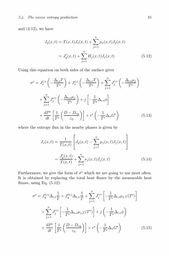
5.4. The excess entropy production 81
and (4.12), we have
Jq(x, t) = T (x, t)Js(x, t) +
n∑
j=1
µj(x, t)Jj(x, t)
= J ′q(x, t) +
n∑
j=1
Hj(x, t)Jj(x, t) (5.12)
Using this equation on both sides of the surface gives
σs = J i,os
(−∆i,sT
T s
)+ Jo,i
s
(−∆s,oT
T s
)+
n∑
j=1
J i,oj
(−∆i,sµj
T s
)
+
n∑
j=1
Jo,ij
(−∆s,oµj
T s
)+ j
[− 1
T s∆i,oφ
]
+dP s
dt
[1
T s
(D −Deq
ε0
)]+ rs
(− 1
T s∆nG
s
)(5.13)
where the entropy flux in the nearby phases is given by
Js(x, t) =1
T (x, t)
Jq(x, t) −n∑
j=1
µj(x, t)Jj(x, t)
=J ′
q(x, t)
T (x, t)+
n∑
j=1
sj(x, t)Jj(x, t) (5.14)
Furthermore, we give the form of σs which we are going to use most often.It is obtained by replacing the total heat fluxes by the measurable heatfluxes, using Eq. (5.12):
σs = J ′i,oq ∆i,s
1
T+ J ′o,i
q ∆s,o1
T+
n∑
j=1
J i,oj
[− 1
T s∆i,sµj,T (T s)
]
+n∑
j=1
Jo,ij
[− 1
T s∆s,oµj,T (T s)
]+ j
(− 1
T s∆i,oφ
)
+dP s
dt
[1
T s
(D −Deq
ε0
)]+ rs
(− 1
T s∆nG
s
)(5.15)
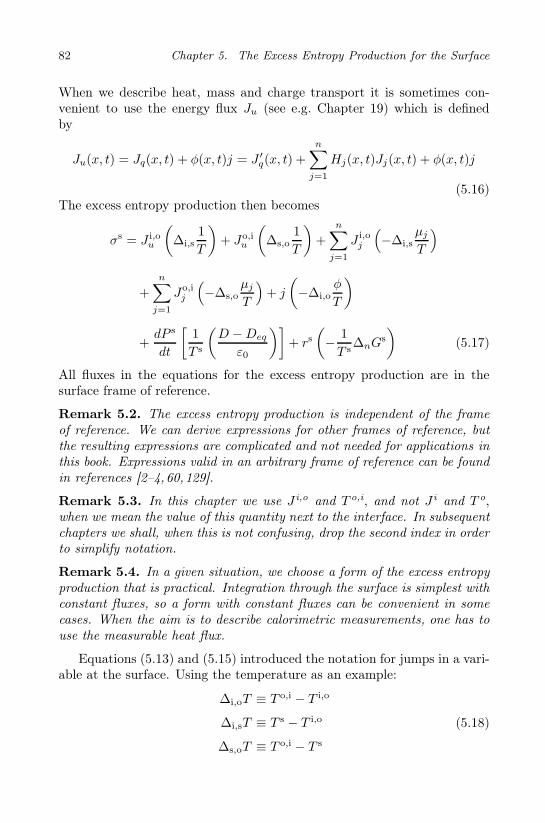
82 Chapter 5. The Excess Entropy Production for the Surface
When we describe heat, mass and charge transport it is sometimes con-venient to use the energy flux Ju (see e.g. Chapter 19) which is definedby
Ju(x, t) = Jq(x, t) + φ(x, t)j = J ′q(x, t) +
n∑
j=1
Hj(x, t)Jj(x, t) + φ(x, t)j
(5.16)The excess entropy production then becomes
σs = J i,ou
(∆i,s
1
T
)+ Jo,i
u
(∆s,o
1
T
)+
n∑
j=1
J i,oj
(−∆i,s
µj
T
)
+
n∑
j=1
Jo,ij
(−∆s,o
µj
T
)+ j
(−∆i,o
φ
T
)
+dP s
dt
[1
T s
(D −Deq
ε0
)]+ rs
(− 1
T s∆nG
s
)(5.17)
All fluxes in the equations for the excess entropy production are in thesurface frame of reference.
Remark 5.2. The excess entropy production is independent of the frameof reference. We can derive expressions for other frames of reference, butthe resulting expressions are complicated and not needed for applications inthis book. Expressions valid in an arbitrary frame of reference can be foundin references [2–4,60,129].
Remark 5.3. In this chapter we use J i,o and T o,i, and not J i and T o,when we mean the value of this quantity next to the interface. In subsequentchapters we shall, when this is not confusing, drop the second index in orderto simplify notation.
Remark 5.4. In a given situation, we choose a form of the excess entropyproduction that is practical. Integration through the surface is simplest withconstant fluxes, so a form with constant fluxes can be convenient in somecases. When the aim is to describe calorimetric measurements, one has touse the measurable heat flux.
Equations (5.13) and (5.15) introduced the notation for jumps in a vari-able at the surface. Using the temperature as an example:
∆i,oT ≡ T o,i − T i,o
∆i,sT ≡ T s − T i,o
∆s,oT ≡ T o,i − T s
(5.18)

5.4. The excess entropy production 83
i os
i,s s,o
i,o o,i
i,o
Figure 5.5 Standard notation for transport across surfaces.
The differences of the surface chemical potentials at constant temperatureare given in terms of the values in the homogeneous phases close to thesurface, in the points a and b, at the temperature of the surface:
∆i,sµj,T (T s) = µsj(T
s) − µi,oj (T s)
∆s,oµj,T (T s) = µo,ij (T s) − µs
j(Ts)
(5.19)
A subscript T indicates a chemical potential difference at a constant surfacetemperature. Each jump is written as the value to the right minus the valueto the left. This choice gives the jumps the same sign as the gradients in thehomogeneous phases for increasing or decreasing variables. The subscriptsof ∆ refer to the two locations between which the difference is taken. Thenotation is further illustrated in Fig. 5.5.
It is interesting to compare Eqs. (5.11), (5.13), (5.15) and (5.17) withEqs. (4.13)–(4.15) and (4.17), that we use for the homogeneous phase. Thegradients of the temperature and the chemical potentials have been replacedby jumps of these variables into and out of the surface, the fluxes are thesame. The gradient of the electric potential has been replaced by a jumpacross the surface. These replacements represent the discrete nature of thesurface and are typical for transport between different homogeneous partsof a system [130].

84 Chapter 5. The Excess Entropy Production for the Surface
Most of the contributions to the excess entropy production of a planar,isotropic surface given above are due to fluxes of heat, mass and charge inthe homogeneous phases outside the surface. The contribution from thechemical reaction is, however, a specific surface contribution. For furtherdetails, we refer to Sec. 7.5 [3, 4, 60, 129]. At the surface, the system isno longer isotropic in the normal direction, so that all the normal fluxes,unlike in a homogeneous phase, are scalar under rotations and reflectionsin the plane of the surface. We therefore have coupling between chemi-cal reactions and such fluxes of heat, mass and charge at a surface. Masstransport fueled by energy from a chemical reaction is called active trans-port in biology [24,52]. The coupling that takes place between scalar fluxesat the surface makes transports in heterogeneous systems different fromtransports in homogeneous system.
We need a common frame of reference for the fluxes when we want todescribe transport in heterogeneous materials. In electroneutral systems,the electric current density, j, is constant throughout the system and inde-pendent of the frame of reference. Mass fluxes, on the other hand, dependon the frame of reference. The frame of reference that gives a simple realis-tic description of the surface is the surface itself. In this frame of reference,the observer moves along with the surface. If the surface is at rest, so is theobserver. This is then also the laboratory frame of reference. It is difficultto describe the surface processes, without using the surface as a frame ofreference. The natural choice of the frame of reference for a heterogeneoussystem is therefore the surface frame of reference. All expressions for theentropy production of the surface, contain fluxes relative to this frame ofreference. We shall proceed to use this frame of reference also for the ad-jacent homogeneous phases, when nothing else is stated. For a definitionof the various frames of reference, and transformations between them, werefer to Sec. 4.4.
The excess entropy production is independent of the frame of reference,and so are the notions, reversible and irreversible. They are in other wordsinvariant under a coordinate transformation. We may therefore convert allfluxes and conjugate forces from any frame of reference to the surface frameof reference and back without changing the entropy productions, σi, σs
and σo.
5.4.1 Reversible processes at the interface and the
Nernst equation
The expression for the excess entropy production contains informationabout the interface at equilibrium. Take as an example an electrode surface.At equilibrium, the excess entropy production is zero. Using Eq. (5.15)

5.4. The excess entropy production 85
as a starting point, we see that the equilibrium conditions are constanttemperature
T o,i = T s = T i,o (5.20)
equilibrium for adsorbed components;
µi,oj (T s) = µs
j(Ts) = µo,i
j (T s) (5.21)
and constant polarizationdP s
dt= 0 (5.22)
During an emf measurement, very small electric currents are passing theelectrode. The constant current means that the electrode reaction is alsoconstant, and rs = j/F. By introducing these conditions into Eq. (5.15) theremaining terms combine to
− [∆i,oφ+ ∆nGs/F ] (j/T s) = 0 (5.23)
meaning that∆i,oφ = −∆nG
s/F (5.24)
The reversible process is characterized by a balance of forces. The electricalforce is balanced by the chemical driving force. The equation is the Nernstequation. It is written for the surface alone. The choice of variables inthe excess entropy production, means that we can calculate the surfacepotential drop, since all contributions to ∆nG
s are well-defined and oftenaccessible in thermochemical tables.
Remark 5.5. The value of ∆i,oφ depends on the standard state that ischosen for the chemical potential of the neutral components. It is thus notan absolute quantity. When the potential difference is calculated betweentwo electrodes, this arbitrariness disappears, if care is taken to use the samestandard states, see Appendix 3.A.
Remark 5.6. The description using absorptions of neutral componentsonly is equivalent to a description using both charged and uncharged compo-nents. This can be seen from the contribution [j(−∆i,oφ) + rs(−∆nG
s)] /T s
when j/F = rs. The difference φo-φi is equal to the Maxwell potential differ-ence ψo- ψi plus the sum of the chemical potentials of the charge carriers di-vided by Faraday’s constant. This gives ∆i,oφ+∆nG
s/F = ∆i,oψ+∆rGs/F
where ∆rGs is the total reaction Gibbs energy, cf. Eq. (5.4). The Nernst
equation for the Maxwell potential difference obtains thereby its more usualform. This shall be shown in Sec. 10.7. See also Appendix 4.A.

86 Chapter 5. The Excess Entropy Production for the Surface
Away from equilibrium also other forces in the expression for σs con-tribute to ∆i,oφ. In addition to a concentration overpotential (µi,o
j (T s) 6=µs
j(Ts)), there can be a thermal overpotential (T o,i 6= T s). The important
reaction overpotential, the resistance of the chemical reaction to chargetransfer, can only be described in its linear regime with the theory of thisbook. In order to describe the activated process with a thermodynamicbasis, we need to introduce so-called internal variables and extend non-equilibrium thermodynamics to the mesoscopic level, cf. Sec. 1.1 [51].
5.4.2 The surface potential jump at the hydrogen electrode
The hydrogen electrode is used to build standard electrochemical tables.The electrode reaction is
1
2H2(g) H+ + e− (5.25)
The standard reduction potential of the hydrogen electrode is set to zero,and other electrode reactions are measured with reference to this value. Atstandard conditions the hydrogen pressure is 1 bar. According to Eq. (5.24),the surface potential jump is given by the standard chemical potential ofhydrogen gas, which is zero by definition
∆a,eφ(H2) = − 1
2Fµ0
H2≡ 0 (5.26)
At any other pressure, the surface potential drop from the anode (a) to theelectrolyte (e) becomes
∆a,eφ(H2) = − 1
2FµH2
= − 1
2F(µ0
H2+RT ln pH2
/p0) (5.27)
This expression shall be used in Chapter 19 to calculate the surface potentialdrop at the anode of the fuel cell. The value of ∆a,eφ(H2) for the anode inthe polymer electrolyte fuel cell, where the electrolyte is an acid membraneis 0.23 V at 340 K and a hydrogen pressure of 0.76 bar, see Figs. 19.3 and19.4.
Out of equilibrium, when the electric current density may become size-able, temperature differences may arise, and the other terms in the entropyproduction may become important. All forces and fluxes in Eq. (5.15)are coupled. The coupling of these phenomena is further described in theapplied part of the book.
Remark 5.7. The advantage of using ∆i,oφ is its relation to measurablequantities, as discussed by Guggenheim [63, 95]. The alternative form of

5.5. Examples 87
the Nernst equation includes chemical potentials of ions, which cannot bemeasured. The meaning of the term −j∆i,oφ comes from Eq. (5.8). Theproduct is the electric work done to the interface when the current j ispassing the cell. In the absence of an external circuit and an electric current,the term disappears from the entropy production.
Remark 5.8. When the standard reduction potential for hydrogen is ex-pressed in terms of the Maxwell potential jump, the convention µ0
H+ +µ0e−
−12µ
0H2
= 0 is used to construct standard tables of reduction potentials.
5.5 Examples
The details of the derivation of the excess entropy production is illustratedby the following exercises.
Exercise 5.5.1. Consider the special case that one component k is trans-ported through an isothermal surface. The densities of the other compo-nents, the internal energy, the molar surface area and the polarizationdensities are all independent of the time. Show that the excess entropyproduction is given by
σs = J i,ok
[− 1
T s
(µs
k − µi,ok
)]+ Jo,i
k
[− 1
T s
(µo,i
k − µsk
)]
• Solution: In this case, Eq. (5.10) reduces to
T s dss
dt+ µs
k
dΓk
dt= 0
The rate of change of the entropy is therefore given by
dss
dt= −µ
sk
T s
dΓk
dt= −µ
sk
T s
(J i,o
k − Jo,ik + rsk
)
where we substituted Eq. (5.3). Setting rsk = 0 one obtains
dss
dt= −µ
sk
T s
(J i,o
k − Jo,ik
)
= −µi,ok
T sJ i,o
k +µo,i
k
T sJo,i
k − J i,ok
(µs
k
T s− µi,o
k
T s
)− Jo,i
k
(µo,i
k
T s− µs
k
T s
)
= J i,os − Jo,i
s + J i,ok
[− 1
T s
(µs
k − µi,ok
)]+ Jo,i
k
[− 1
T s
(µo,i
k − µsk
)]
By comparing this equation with Eq. (5.1), we can identify the wantedexcess entropy production.

88 Chapter 5. The Excess Entropy Production for the Surface
Exercise 5.5.2. Consider the special case that only heat is transported.Show that the excess entropy production is given by
σs = J ′i,oq
(1
T s− 1
T i,o
)+ J ′o,i
q
(1
T o,i− 1
T s
)
• Solution: In this case Eq. (5.10) reduces to
dus
dt= T sds
s
dt.
The rate of change of the entropy is therefore given by
dss
dt=
1
T s
dus
dt.
Eq. (5.8) reduces todus
dt= J ′i,o
q − J ′o,iq
By combining the three equations, we obtain
dss
dt=
1
T s
(J ′i,o
q − J ′o,iq
)
=1
T i,oJ ′i,o
q − 1
T o,iJ ′o,i
q + J ′i,oq
(1
T s− 1
T i,o
)+ J ′o,i
q
(1
T o,i− 1
T s
)
= J i,os − Jo,i
s + J ′i,oq
(1
T s− 1
T i,o
)+ J ′o,i
q
(1
T o,i− 1
T s
)
By comparing this equation with Eq. (5.1), we can identify the excessentropy production.
Exercise 5.5.3. Consider stationary state evaporation of A from a solu-tion. The flux is 1.6 10−6 mol/m2s. The other component does not evap-orate. The concentrations close to the surface are ciA = 0.05 kmol/m−3
on the liquid side, and coA = 0.01 kmol/m−3 on the gas side. What is theexcess entropy production in the surface?
• Solution: At stationary state, there is no accumulation of A in thesurface and J i,o
A = Jo,iA . When the temperature is constant, the excess
entropy production is
σs = J i,oA
[− 1
T s(µs
A − µi,oA )
]+ Jo,i
A
[− 1
T s(µo,i
A − µsA)
]
= JA
[− 1
T s
(µo,i
A − µi,oA
)]= JAR ln
ciAcoA
= 2.1 × 10⁻⁵ W/Km2

5.5. Examples 89
The excess entropy production is no direct function of the tempera-ture. In order to compare the surface excess entropy production tothe one in homogeneous phases, we divide this value with the thick-ness of the surface, which is order of magnitude 10−9 m. The resultis very large compared to i.e. the one we calculated in Exercise 4.3.3.This shows that the interface is relatively speaking the source of muchentropy production.
Exercise 5.5.4. Derive Eq. (5.15) from Eq. (5.11).
• Solution: We have
∆i,s
(µj
T
)=µs
j(Ts)
T s−µi,o
j (T i,o)
T i,o
=µs
j(Ts)
T s−µi,o
j (T s)
T s+µi,o
j (T s)
T s−µi,o
j (T i,o)
T i,o
=1
T s∆i,sµj,T +
(∂
∂T
µi,oj
T
)
T=T i,o
(T s − T i,o)
=1
T s∆i,sµj,T −
(1
T i,oSi,o
j +µi,o
j
(T i,o)2
)(T s − T i,o)
=1
T s∆i,sµj,T +
(Si
j +µi,o
j
T i;o
)T s∆i,s
(1
T
)
=1
T s∆i,sµj,T +H i,o
j
(T s
T i,o
)∆i,s
(1
T
)
We can assume that, T s ≈ T i, so that
∆i,s
(µj
T
)=
1
T s∆i,sµj,T +H i,o
j ∆i,s
(1
T
)
By substituting this result, and the analogous result for the other sideof the surface, for all components into Eq. (5.11), using the definitionof the measurable heat fluxes on both sides, we obtain Eq. (5.15).

This page intentionally left blankThis page intentionally left blank
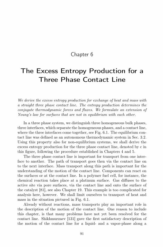
Chapter 6
The Excess Entropy Production for a
Three Phase Contact Line
We derive the excess entropy production for exchange of heat and mass witha straight three phase contact line. The entropy production determines theconjugate thermodynamic forces and fluxes. We formulate an extension ofYoung’s law for surfaces that are not in equilibrium with each other.
In a three phase system, we distinguish three homogeneous bulk phases,three interfaces, which separate the homogeneous phases, and a contact line,where the three interfaces come together, see Fig. 6.1. The equilibrium con-tact line was defined as an autonomous thermodynamic system in Sec. 3.2.Using this property also for non-equilibrium systems, we shall derive theexcess entropy production for the three phase contact line, denoted by c inthis figure, following the procedure established in Chapters 4 and 5.
The three phase contact line is important for transport from one inter-face to another. The path of transport goes then via the contact line onto the next interface. Mass transport along this path is important for theunderstanding of the motion of the contact line. Components can react onthe surfaces or at the contact line. In a polymer fuel cell, for instance, thechemical reaction takes place at a platinum surface. Gas diffuses to theactive site via pore surfaces, via the contact line and onto the surface ofthe catalyst [81], see also Chapter 19. This example is too complicated foranalysis here, however. We shall limit ourselves to transport of heat andmass in the situation pictured in Fig. 6.1.
Already without reactions, mass transports play an important role inthe description of the motion of the contact line. One reason to includethis chapter, is that many problems have not yet been resolved for thecontact line. Shikhmurzaev [131] gave the first satisfactory description ofthe motion of the contact line for a liquid- and a vapor-phase along a
91

92 Chapter 6. The Excess Entropy Production for a Three Phase Contact Line
c
r
φ
Figure 6.1 The geometry around the contact line, c. The distance to the lineis r, and φ is the angle around the line.
flat solid wall. He used non-equilibrium thermodynamics for the surfacesfollowing, and extending, the method of Bedeaux et al. [2]. He described thecontact line, choosing boundary conditions for the surfaces at the contactline. We shall generalize Shikhmurzaev’s analysis by treating the contactline as a thermodynamic system. The excess entropy production along theline gives a proper basis for the boundary conditions to be chosen. We referto Bedeaux [132] for a more detailed presentation.
6.1 The discrete nature of the contact line
The excess densities of the contact line were described in Sec. 3.2. Theseapply to a point on the contact line. In order to write balance equations forthe line, we need to consider its surroundings. We introduce a coordinatec along the line, a distance r to the contact line and an angle ϕ aroundthe contact line, see Fig. 6.1. Close to the contact line these are cylindricalcoordinates∗. We assume that the contact line is straight and that theinterfaces are flat. Furthermore, we restrict ourselves to the case that alldensities and fluxes are independent of c, and that there are no fluxesparallel to the contact line, neither in the homogeneous phases, nor alongthe surfaces. This is appropriate for exchange of heat and mass with thecontact line. We recommend to use the symbol list for a check of thedimensions in the equations.
∗Farther away from and along the contact line, one should in the general case useorthonormal curvilinear coordinates, see Refs. [2–4].

6.1. The discrete nature of the contact line 93
The balance equation for the excess entropy density sc of the contactline is:
d
dtsc +
3∑
ν=1
Js,νs .nν =
d
dtsc +
3∑
ν=1
J s,νs,r = σc (6.1)
The indices ν = 1, 2 and 3 label the homogeneous phases, counted clockwisearound the contact line, and the surfaces, counted clockwise around thecontact line, respectively. The first surface comes after the first bulk phase,etc. Js,ν
s are the excess entropy fluxes along the dividing surfaces. Thenormal to the contact line, that is directed away from the contact linein the ν-th interface, is denoted nν . We use a subscript r to label thecomponent of the flux along the interface normal to the contact line.
Remark 6.1. In Chapter 5, we did not consider excess fluxes along thesurface. In this chapter only these fluxes give exchange of heat and masswith the contact line. Excess fluxes along the surfaces are defined in thesame way as the excess densities for the surfaces in Sec. 3.2.
The excess entropy fluxes are given in terms of the total excess heatfluxes, the excess measurable heat fluxes and the excess mass fluxes alongthe surfaces by
Js,νs =
1
T s,ν
Js,ν
q −n∑
j=1
µs,νj J
s,νj
=
1
T s,νJ′,s,ν
q +n∑
j=1
Ss,νj J
s,νj (6.2)
All fluxes are given in the contact line frame of reference (the contact lineis not moving):
vcj = vc
j,r = vc = vcr = 0 (6.3)
The time derivative d/dt in Eq. (6.1), is in this frame of reference. It isappropriate to use d/dt because the excess entropy density depends onlyon the time. The definition of excess densities for the contact line wasdiscussed in Sec. 3.2.
The second law gives for the contact line σc (t) ≥ 0. We shall find moreexplicit expressions for σc(t) by combining:
• mass balances
• the first law of thermodynamics
• the local form of the Gibbs equation
The same procedure was used in Chapters 4 and 5. We shall see that alsoσc(t) can be written as the product sum of conjugate fluxes and forces forthe contact line. The fluxes and forces describe exchange of heat and massbetween the contact line and the surfaces.

94 Chapter 6. The Excess Entropy Production for a Three Phase Contact Line
6.2 Balance equations
Conservation of component j along a contact line gives
ddt
Γcj = −
3∑
ν=1
Js,νj .nν = −
3∑
ν=1
J s,νj,r (6.4)
where Γcj are the excess line concentrations (adsorptions per unit of length).
Furthermore J s,νj,r is the excess flux of component j along the surface ν away
from the contact line, see Fig. 6.1. The adsorptions depend only on the time.
With the chosen frame of reference, the velocity of the line is zero, butthe line can be accelerated in the plane normal to the line. For such acomoving acceleration, we have
d
dt(mcΓcvc
⊥) =3∑
ν=1
(γν −mνΓνvs,νr vs,ν
r ) nν (6.5)
where mcΓc and mνΓν are the average excess mass densities per unit oflength along the contact line and along the dividing surfaces, respectively.They are defined by
mcΓc ≡n∑
j=1
mjΓcj and mνΓν ≡
n∑
j=1
mjΓνj (6.6)
The barycentric velocities along the dividing surfaces, vs,ν are:
mνΓνvs,ν ≡n∑
j=1
mjJs,νj ≡
n∑
j=1
mjΓνj v
s,νj (6.7)
The first term on the right hand side of Eq. (6.5), gives the terms thatappear in Young’s law for a contact line. The second term gives a convectivecorrection to this law, needed in the non-equilibrium case.
Conservation of excess internal energy density, uc, per unit of lengthmeans that:
d
dtuc = −
3∑
ν=1
Js,νq .nν = −
3∑
ν=1
J s,νq,r (6.8)
The excess total heat fluxes are given in terms of the excess measurableheat fluxes along the interfaces:
Js,νq = J′,s,ν
q +
n∑
j=1
Hs,νj J
s,νj (6.9)

6.3. The excess entropy production 95
where Hs,νj are the partial molar excess enthalpies along the dividing
surfaces.
Remark 6.2. In Eqs. (6.1), (6.4) and (6.8) there are no direct fluxesfrom the homogeneous phases to the contact line. The geometry around thecontact line is such that such fluxes would diverge inversely proportional tothe distance to the contact line. As a consequence such fluxes are impossible.
This property has a bearing on the gas transport to the three phasecontact line that we discuss in Chapter 21. Transport occurs via the planes.
6.3 The excess entropy production
We assume that there is local equilibrium everywhere along the contactline. The Gibbs equation (3.33) for the line gives:
T c dsc
dt=
duc
dt−
n∑
j=1
µcj
dΓcj
dt(6.10)
We substitute Eqs. (6.4) and (6.8) into this equation. By using Eq. (6.2) andcomparing the result with Eq. (6.1), we can identify the entropy production:
σc =
3∑
ν=1
J s,νq,r
(1
T s,ν− 1
T c
)−
3∑
ν=1
n∑
j=1
J s,νj,r
(µs,ν
j
T s,ν−µc
j
T c
)(6.11)
This is caused by transport of heat and mass into and out of the contactline. The force-flux pairs have a similar form as for the surface. By usingEq. (6.2), we can eliminate the total heat fluxes in terms of the entropyfluxes
σc =3∑
ν=1
T s,νJ s,νs,r
(1
T s,ν− 1
T c
)− 1
T c
3∑
ν=1
n∑
j=1
J s,νj,r
(µs,ν
j − µcj
)(6.12)
By using Eq. (6.9), we can eliminate the total heat fluxes in terms of themeasurable heat fluxes
σc =
3∑
ν=1
J ′,s,νq,r
(1
T s,ν− 1
T c
)
−3∑
ν=1
n∑
j=1
J s,νj,r
[(µs,ν
j
T s,ν−µc
j
T c
)−Hs,ν
j
(1
T s,ν− 1
T c
)]
=
3∑
ν=1
J ′,s,νq,r
(1
T s,ν− 1
T c
)− 1
T c
3∑
ν=1
n∑
j=1
J s,νj,r
(µs,ν
j (T c) − µcj
)(6.13)

96 Chapter 6. The Excess Entropy Production for a Three Phase Contact Line
All contributions are scalar. When there are fluxes along the contact line[132], additional terms appear in Eq. (6.13). Gradients in temperature andabsorption along the line, which were not considered in the analysis above,result in a so-called Marangoni effect. The so-called tears of wine are anexample of the Marangoni effect for a surface. Take a glass of strong portwine. When one wets a part of the surface with the port, tears will appearalong the contact line between the dry and the wet surface. This is due toevaporation of alcohol, which increases the surface tension close to the line.The tears grow until they become so heavy that they fall down along thesurface of the glass.
6.4 Stationary states
Stationary state conditions reduce the number of independent flux-forcepairs significantly, from 3(n + 1) to 2(n + 1). In a stationary state, theconservation equation for component j in the contact line, Eq. (6.4), reducesto
3∑
ν=1
J s,νj,r = 0 (6.14)
There is mechanical equilibrium in the direction normal to the contact line.This gives, from Eq. (6.5)
3∑
ν=1
γνnν = 0 (6.15)
for sufficiently low velocities along the surfaces. This is Young’s law forsurfaces which are not in equilibrium with each other. The contact anglesin the formula deviate from their equilibrium values. The balance of internalenergy, Eq. (6.8), reduces to
3∑
ν=1
J s,νq,r = 0 (6.16)
Using Eqs. (6.14) and (6.16), the excess entropy production along the con-tact line can be written as
σc =
2∑
ν=1
J s,νq,r
(1
T s,ν− 1
T s,3
)−
2∑
ν=1
n∑
j=1
J s,νj,r
(µs,ν
j
T s,ν−µs,3
j
T s,3
)(6.17)
This reduces the number of independent force-flux pairs from 3(n + 1) to2 (n+ 1). A simplification is also that the thermodynamic forces no longerdepend on the temperature and the chemical potentials along the contact
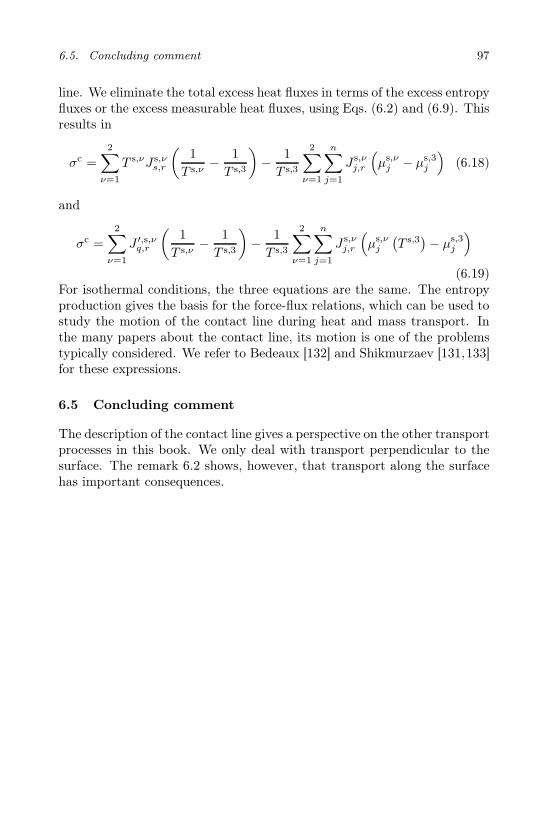
6.5. Concluding comment 97
line. We eliminate the total excess heat fluxes in terms of the excess entropyfluxes or the excess measurable heat fluxes, using Eqs. (6.2) and (6.9). Thisresults in
σc =2∑
ν=1
T s,νJ s,νs,r
(1
T s,ν− 1
T s,3
)− 1
T s,3
2∑
ν=1
n∑
j=1
J s,νj,r
(µs,ν
j − µs,3j
)(6.18)
and
σc =2∑
ν=1
J ′,s,νq,r
(1
T s,ν− 1
T s,3
)− 1
T s,3
2∑
ν=1
n∑
j=1
J s,νj,r
(µs,ν
j
(T s,3
)− µs,3
j
)
(6.19)For isothermal conditions, the three equations are the same. The entropyproduction gives the basis for the force-flux relations, which can be used tostudy the motion of the contact line during heat and mass transport. Inthe many papers about the contact line, its motion is one of the problemstypically considered. We refer to Bedeaux [132] and Shikmurzaev [131,133]for these expressions.
6.5 Concluding comment
The description of the contact line gives a perspective on the other transportprocesses in this book. We only deal with transport perpendicular to thesurface. The remark 6.2 shows, however, that transport along the surfacehas important consequences.

This page intentionally left blankThis page intentionally left blank

Chapter 7
Flux Equations and Onsager Relations
We present the flux equations that follow from the entropy production on ageneral form. Onsager’s proof for the reciprocal relations is discussed. Thevalidity of the Onsager relations assures that, in the absence of constraints,the system relaxes to equilibrium. The second law leads to restrictions onthe transport coefficients. In the stationary state, it is an advantage towrite the forces as functions of fluxes. The meaning of the Curie principleis discussed for surfaces and contact lines.
This chapter gives the general properties of the flux-force equations innon-equilibrium thermodynamics. The properties are not only applicable tothe phenomena treated in this book, they are also valid for phenomena thatwe omit, like for instance viscous flow. Explicit expressions for transportof heat, mass and charge in two flux-two force systems follow in Chapters8–10. After that we go to more complicated applications.
7.1 Flux-force relations
As explained in Chapter 1, non-equilibrium thermodynamics has as basisthe entropy production, which has the general form
σ =
n∑
i=1
JiXi (7.1)
where Ji and Xi are the so-called conjugate thermodynamic fluxes andforces, cf. Eq. (1.4). There are n independent flux-force pairs. The con-jugate pairs were derived in Chapters 4–6. The meaning of being conju-gate shall be further discussed in the next section. A basic assumption in
99

100 Chapter 7. Flux Equations and Onsager Relations
non-equilibrium thermodynamics is that each flux is a linear function of allforces:
Ji =n∑
j=1
LijXj (7.2)
The relationship is linear in the sense that the Onsager conductivity matrixLij does not depend on Xj . The coefficients are functions of the statevariables, for instance, like the local pressure and temperature, but not ofthe forces. The theory therefore prescribes that coefficients, like the thermalconductivity, can depend on the temperature, but not on the gradient ofthe temperature.
7.2 Onsager’s reciprocal relations
Onsager [8, 9] showed that the matrix of coefficients for Eq. (7.2) is sym-metric, using the microscopic time reversibility of the system. Consider,as Onsager did, a system described by thermodynamic variables Ai whichare symmetric (even) with respect to reversal of the time. Examples of Ai
are the internal energy density and the molar densities of volume elementsin the homogeneous phases, of area elements along the dividing surfaces,and of length elements along the contact line. The fluctuations αi of thethermodynamic variables Ai are defined by:
αi ≡ Ai− < Ai > (7.3)
Microscopic reversibility means that the probability to observe, on the aver-age, that a fluctuation αi in some property at time t, is followed by anotherfluctuation αj after a time lag τ , is equal to the probability to observe thereverse situation — that the fluctuation αj at time t, is followed by αi aftera time lag τ . Mathematically this implies that:
< αi(t)αj(t+ τ) >=< αj(t)αi(t+ τ) > (7.4)
where the brackets < ... > mean that averages have been calculated overthe equilibrium distribution given in Eq. (7.7), see Eq. (7.11) for an explicitdefinition of such an average. Microscopic time reversibility is a character-istic property of Newton’s equations. The motion of a particle in a fluidaccording to Newton’s equations is illustrated in Sec. 22.1, Fig. 22.1.
The entropy of the system, S, has a maximum, Seq, at equilibrium.Away from equilibrium it is:
S = Seq + ∆S(α1, ..., αn) = Seq −1
2
n∑
j,i=1
gjiαjαi + ... (7.5)

7.2. Onsager’s reciprocal relations 101
where ∆S describes the deviation∗ from the equilibrium value. The tensorgji is defined by the elements
gji ≡ − ∂2∆S
∂αj∂αi
∣∣∣∣α1=...=αn=0
(7.6)
As Seq is a maximum, there is no linear term in the expansion. Furthermore,gji is a positive definite and real symmetric matrix. It follows that theeigenvalues are all real and positive. We can choose the amplitudes of theeigenvectors divided by the square root of their eigenvalues as a new set ofvariables α′
i. The resulting g′ji is then equal to the unit tensor.From Boltzmann we have the normalized probability density for the
fluctuations:
f(α1, ..., αn) = exp (∆S/kB) /
∫ ∞
−∞
dα1...dαn exp (∆S/kB) (7.7)
where kB is the Boltzmann constant. The integral is taken over all nfluctuation variables. The thermodynamic forces Xi in the system weredefined by Onsager:
Xi ≡∂S
∂Ai=∂∆S
∂αi= −
n∑
j=1
gijαj + ... (7.8)
Here we used ∆S as given in Eq. (7.5). The conjugate fluxes were definedby:
Ji(t) =dAi(t)
dt=dαi(t)
dt(7.9)
From Eqs. (7.7) and (7.8) we have:
Xi = kB∂ ln f
∂αi=kB
f
∂f
∂αi(7.10)
Using the definition of Xi and partial integration, it follows that the expec-tation value of the product αiXj is
< αiXj >≡∫ ∞
−∞
dα1...dαn αiXj f(α1, ..., αn) = −kBδij (7.11)
where δij is the Kronecker delta, δij ≡ 1 if i = j and δij ≡ 0 if i 6= j.On a microscopic time scale one observes collisions between particles.
Figure 22.1 shows the path of one particle in a fluid. A discontinuity in∗The deviation ∆S is not necessarily a quadratic form of the fluctuations, see [20]
p. 91, as is frequently assumed.

102 Chapter 7. Flux Equations and Onsager Relations
the path means that a collision takes place. A collision leads to a rapidchange in the variables αi. In order to find the macroscopic behavior, onemust integrate over a sufficiently long time to no longer see these rapidchanges. The rapid fluctuations have then re-established the equilibriumdistribution. The time needed depends on the system under consideration.It can be vastly different for a chemical reaction, for a diffusing polymer orfor a diffusing argon fluid such as the one in Fig. 22.1. Onsager assumedthat the microscopic fluctuation in αi and the flux Ji obeyed the linearmacroscopic relation given in Eq. (7.2):
Ji(t) =
n∑
j=1
LijXj(t) (7.12)
This is called the regression hypothesis. By integrating Eq. (7.9) from t tot+ τ , using Eq. (7.12), he then found that:
αi(t+ τ) = αi(t) + τ
n∑
j=1
LijXj(t) (7.13)
to linear order in τ . By introducing Eq. (7.13) on both sides of Eq. (7.4)using Eq. (7.11), the reciprocal relations followed.
Lij = Lji (7.14)
These are the Onsager relations for conductivity coefficients. They makethe matrix of the coefficients in the flux equations symmetric†. The On-sager relations simplify the transport problem greatly, because they reducethe number of independent conductivity coefficients from n2 to 1
2n(n+ 1).When the Onsager coefficients Lij are known, we know how the differentprocesses are coupled to one another. We can even take advantage of thesituation to find thermodynamic data which are otherwise difficult to mea-sure, see Ref. [76]. The coefficients must be determined from experiments.The Onsager relations have been verified experimentally for many systems[71–74]. They have also been verified by non-equilibrium molecular dynam-ics simulations [65, 67].
Let us summarize the conditions for validity of Onsager’s reciprocalrelations, Eq. (7.14):
• The state variables Ai(t) are independent.
†When odd variables are used in combination with even variables, the correspondingcoupling coefficents become antisymmetric [20].

7.2. Onsager’s reciprocal relations 103
• The fluxes and forces are conjugate; i.e. for each variable Ai(t), aflux is defined as dαi(t)/dt and the conjugate force is defined asd∆S/dαi.
• The fluxes are linear functions of the conjugate thermodynamic forces.The coefficients Lij may therefore depend on the state variables, butnot on the forces.
Freedom exists, as is normal in thermodynamics, to choose alternative setsof variables. Choosing different variables changes the αi’s and accordinglymodifies the fluxes and the conjugate forces. Onsager’s prescription makesclear how to find the conjugate flux-force pairs. Regretfully enough, On-sager’s analysis and the consequences thereof have been presented in a mis-leading manner, for instance by Coleman and Truesdell [134] and Wei [135],questioning their validity and/or usefulness. For a discussion of the pointsraised by these authors, see de Groot and Mazur [20] Sec. VI.5.
When the set of variables Ai(t) is overcomplete, it can be shown that asymmetric coefficient matrix can be chosen, see [20] Sec. VI.3. The set ofindependent Ai(t) leads to the smallest number of independent phenomeno-logical coefficients and is usually most efficient. The Maxwell–Stefan for-mulation is an important exception to this, see Sec. 12.2.
The equations that describe the dynamics of the system are non-linear.To refer to non-equilibrium thermodynamics as a linear theory, as is oftendone [64], is therefore misleading. De Groot and Mazur pointed out in thepreface to the Dover edition of their monograph [20], that these equationsare “non-linear for a variety of reasons, such as (i) the presence of convec-tion terms and of (ii) quadratic source terms in, e.g. the energy equation,(iii) the non-linear character of the equation of state and (iv)the dependence of the phenomenological transport coefficients on thestate variables”.
To illustrate the non-linearity of the equations by an example, considerthe dynamics of an isothermal fluid. The dynamics is described by thecontinuity equation and the Navier–Stokes equation, classical examples ofnon-linear equations. The phenomenological coefficients, giving the lineardissipative contributions to the fluxes, are the shear viscosity and the bulkviscosity. For large Reynolds numbers the viscous contributions can beneglected and the equations reduce to the Euler equation. These equationsdescribe classic non-linear reversible flow phenomena, like turbulence, andhave Lij = 0. The transition to turbulence in a fluid is therefore not dueto the appearance of contributions in the fluxes which are non-linear in thethermodynamic forces. On the contrary, the dissipative contributions tothe fluxes in the Euler equations are in fact negligible.

104 Chapter 7. Flux Equations and Onsager Relations
Exercise 7.2.1. Derive Eq. (7.11) from Eqs. (7.3) to (7.8).
• Solution: Using Eq. (7.8) we have
< αiXj > ≡∫ ∞
−∞
dα1...dαn αiXj f(α1, ..., αn)
= kB
∫ ∞
−∞
dα1...dαn αi∂lnf
∂αjf(α1, ..., αn)
= kB
∫ ∞
−∞
dα1...dαn αi∂
∂αjf(α1, ..., αn)
We use∂
∂αjαif = αi
∂f
∂αj+ f
∂αi
∂αj= αi
∂f
∂αj+ fδij
to find an expression for αi (∂f/∂αj). The integral contains two partsthat can be integrated separately. We use the normalization conditionfor f and the fact that f goes to zero for large values of the fluctuationsand obtain:
< αiXj >≡ kB
∫ ∞
−∞
dα1...dαn
[∂
∂αjαif − fδij
]= −kBδij
Exercise 7.2.2. Onsager chose the time a particle needs to diffuse over itsown diameter as a measure of the time the system takes to come to localequilibrium (and for Eq. (7.12) to apply). Suggest a way to estimate thistime to about 10−6s.
• Solution: The time is given by the diameter squared divided by thediffusion constant (see Sec. 8.2). A diameter of 0.5 nm and a diffusionconstant of 2.5 × 10⁵(nm)2/s gives the time 10−6 s.
7.3 Relaxation to equilibrium. Consequences of violating
Onsager relations
Thermodynamic systems will always go to equilibrium, when the system isclosed. The reason for this is that Onsager relations are valid. We illustratebelow in an exercise, that a violation of the Onsager relations may leadto oscillatory behavior around the equilibrium state. Equilibrium is thennever reached.
We show first why an isolated system always approaches equilibrium.Consider variables that make gji equal to the unit tensor. Below Eq. (7.6)

7.4. Force-flux relations 105
we explained why the system can be described in terms of such variables.It then follows from Eq. (7.8) that Xi = −αi. Close to equilibrium wemay neglect possible higher order contributions. Equation (7.2) then gives,using Eq. (7.9) for the time derivative of αi,
dαi
dt= −
n∑
j=1
Lijαj (7.15)
When one diagonalizes the matrix of conductivities, it follows from the On-sager reciprocal relations that all the eigenvalues are real and non-negative.As a consequence the system will go to equilibrium.
The following exercise illustrates what goes wrong when the phenomeno-logical coefficient are chosen such that they neither satisfy the Onsager re-lations nor the inequalities which follow from the second law (see Sec. 7.5).
Exercise 7.3.1. Consider a system described by Eq. (7.15) with two forcesand fluxes. Use L11 = L22 = 0 and L12 = −L21. Calculate α1(t) using theinitial value α1(0) = A and (dα1/dt)(t = 0) = 0.
• Solution: Equation (7.15) gives dα1/dt = −L12α2 and dα2/dt =L12α1. The second derivative of α1 becomes d2α1/dt
2 = −L12dα2/dt = −L2
12α1. The solution of this equation for the given initialconditions is α1(t) = A cos(L12t).
The system in the exercise has an oscillating solution, which does not goto equilibrium.
Remark 7.1. Onsager’s relations provide the general reason why oscil-lating behavior around equilibrium does not exist in systems described bynon-equilibrium thermodynamics.
When there are external forces which bring the system far away from equi-librium, for instance by keeping one of the variables constant, the propertiesof the system change, see Prigogine and coworkers [136]. Multiple station-ary states may then exist and oscillatory and more complex behavior candevelop. But that is not the subject of this book.
7.4 Force-flux relations
In the inverted form of Eq. (7.2), the forces are linear functions of the fluxes:
Xi =
n∑
j=1
RijJj (7.16)

106 Chapter 7. Flux Equations and Onsager Relations
The resistivity matrix, Rij , is the inverse of the conductivity matrix:
n∑
j=1
RijLji = δij (7.17)
In stationary states the fluxes are often constant in space. The force-fluxrelations are then particularly convenient. We use Kramer’s rule to findthe matrix elements. An element Rij in the resistivity matrix is equalto the subdeterminant of the conductivity matrix (the determinant of thematrix in which the ith row and the jth column have been crossed out, times(−1)i+j , divided by the determinant of the conductivity matrix). For n = 2,we find
R11 =L22
L11L22 − L212
, R12 = R21 = − L12
L11L22 − L212
,
R22 =L11
L11L22 − L212
(7.18)
The matrix of resistivity coefficients satisfies the Onsager reciprocal rela-tions, just like the matrix of conductivity coefficients:
Rij = Rji (7.19)
7.5 Coefficient bounds
The second law imposes certain bounds on the Onsager coefficients. Bysubstituting the linear laws into σ, we have:
σ =∑
i
Xi
∑
j
LijXj =∑
i,j
XiLijXj ≥ 0 (7.20)
The second law gives the inequality. By taking all forces, except one, equalto zero, it follows that main coefficients are always positive
Lii ≥ 0 (7.21)
A consequence of the second law of thermodynamics is also that all pairsof coefficients obey:
LiiLjj − LijLji ≥ 0 (7.22)

7.5. Coefficient bounds 107
This can be found by taking all except two forces equal to zero, and sub-sequently eliminating one of the two forces in terms of the correspondingflux. We have
J1 = L11X1 + L12X2
J2 = L21X1 + L22X2
(7.23)
By eliminating X2 in the first equation by means of the second, we obtain
J1 =
(L11 −
L12L21
L22
)X1 +
L12
L22J2 (7.24)
When this is introduced into the entropy production, we find:
σ =
(L11 −
L12L21
L22
)X2
1 +L12
L22J2X1 −
L21
L22J2X1 +
J22
L22
=
(L11 −
L12L21
L22
)X2
1 +J2
2
L22(7.25)
Two of the terms cancel because of the Onsager relation, Eq. (7.14). Wemust have σ ≥ 0, also for the special case that J2 = 0. Equations (7.22)follow from this. It is interesting to note that by keeping the flux J2 ratherthan the force X2 equal to zero, the entropy production is reduced fromL11X
21 to (L11 − L12L21/L22)X
21 .
Remark 7.2. When X1 = 0, a finite flux J2 gives rise to a flux J1 =(L12/L22)J2, see Eq. (7.24). The expression for the entropy production,Eq. (7.25), shows, however, that this contribution to J1 does not contributeto the entropy production. This transport along with J2 is therefore re-versible. The coupling coefficients therefore describe reversible contributionsto σ. This is why they are important for a proper description of energy con-version, cf. Secs. 2.1, 9.3, 9.4, 10.1 and 10.6.
An equality sign in Eq. (7.22) implies that two fluxes are proportional toone another. In our example, J1 = (L12/L22)J2. This is called completecoupling. A consequence is that the number of fluxes, and therefore thenumber of variables, can be reduced.
For the force-flux relations we find, by substituting Eq. (7.16) intoEq. (1.1):
σ =∑
i
Ji
∑
j
RijJj =∑
i,j
JiRijJj ≥ 0 (7.26)

108 Chapter 7. Flux Equations and Onsager Relations
The second law gives now:Rii ≥ 0 (7.27)
andRiiRjj −RijRji ≥ 0 (7.28)
The resistivity coefficients have similar properties as the conductivitycoefficients.
7.6 The Curie principle applied to surfaces and contact lines
As we go from a three-, to a two-, and a one-dimensional phase, the sym-metry properties of the phases are gradually reduced. Symmetry propertiesrestrict the possibilities for coupling between transport phenomena. Thiswas first recognized by Pierre Curie [137], and has been referred to as theCurie principle.
Transport phenomena are scalar, vectorial or tensorial. Chemical re-actions are scalar, and are classified with a tensorial rank 0. Vectorialheat-, mass-, and charge transport have rank 1. Momentum transport isa tensorial phenomenon of rank 2. Curie saw that components of differentrank tensors have different transformation properties under rotations andreflections of the system. The entropy production (4.13)–(4.15) for the ho-mogeneous phase used in this book, contains phenomena of two tensorialranks, scalar chemical reactions and vectorial transports of heat, mass andcharge. There is no coupling between chemical reactions and the vecto-rial phenomena in the homogeneous phase. De Groot and Mazur [20] dis-cussed coupling in homogeneous phases from this perspective, see Sec. VI, 2;page 57.
The symmetries change when we consider the surface. The surface canbe symmetric for two-dimensional transformations along the surface, but ithas no symmetries in the direction normal to the surface. A surface is calledisotropic when it is invariant for rotations around, and reflections with re-spect to any normal. Scalar phenomena in the homogeneous regions havetheir scalar counterpart at the surface, the typical example being chemicalreactions. Vectorial phenomena in the homogeneous region must be splitinto the projection along the surface, and the component normal to thesurface. In the excess entropy production of the surface, see Eqs. (5.11),(5.13) and (5.15), the 2-dimensional projection of the 3-dimensional vec-torial flux or force, has the same symmetry as vectorial fluxes and forcesalong the surface. The normal component of the 3-dimensional vector hasthe symmetry of a scalar along the surface. Similarly, a 3×3 tensor in thehomogeneous phase, gives a 2×2 tensor, two 2-dimensional vectors and onescalar along the surface.

7.6. The Curie principle applied to surfaces and contact lines 109
We are dealing in this book with one-dimensional transport processeswith a direction normal to the surface. All contributions to the excessentropy production of the surface are therefore scalar, they are chemicalreactions or normal components of 3-dimensional vectors. The importantconsequence is that coupling is possible between the chemical forces andelectrical, thermal and diffusional forces into or across the surface. Thispossibility was pointed out by Bertrand and Prud’homme [59, 60] and Be-deaux and coworkers [2, 4]. We shall elaborate on this in the followingchapters. The coupling between the chemical reaction and the electric po-tential jump at the surface is a large effect, leading for instance to theNernst equation for the surface, see Secs. 5.4 and 10.7. It is known frombiology, that chemical reaction energy can be transformed to give directedtransport across a membrane (so-called active transport, see [23, 24, 52]).This type of coupling is possible only at the membrane surface, accordingto the Curie principle.
The three phase contact line has only scalar contributions to its excessentropy production, Eqs. (6.11)–(6.13). All these scalar fluxes may cou-ple. The normal component of an excess vectorial flux along the two-phasesurfaces at the contact line, will for instance, couple to a chemical reac-tion along the line. This may have a bearing on electrochemical reactions,which often take place between reactants and products that are distributedin different phases, see Chapters 10, and 13–17.

This page intentionally left blankThis page intentionally left blank

Chapter 8
Transport of Heat and Mass
We present flux equations for transport of heat and mass in a simple het-erogeneous system. Transport coefficients for homogeneous phases havebeen measured or modeled. We give the Onsager coefficients in terms ofsuch coefficients.
Heat and mass transport is central in mechanical as well as in chem-ical engineering. Several books have been written on such transports,e.g. [69, 84, 138]. Also, in nature there are frequently temperature anddensity gradients, and as a consequence, transport of heat and mass. Ourpresentation aims to add to these descriptions, by giving complete setsof transport coefficients for heterogeneous systems. Onsager coefficients forheat and mass transfer shall be specified, both for the homogeneous regionsand for the surfaces between them. They shall also be related to measuredcoefficients, like the thermal conductivity, the diffusion coefficient and theSoret coefficient.
We consider the simplest heterogeneous system to bring out the physicalphenomena; a series of two homogeneous phases and a flat surface betweenthem. We are concerned with transport of heat and one component in thedirection normal to the surface. The other component is not moving andis used as the frame of reference. The dividing surface is defined as theequimolar surface of this component and is also not moving. The descrip-tion in terms of the measurable heat flux, J ′
q, and the molar flux of themoving component, Jm, brings out the importance of the enthalpy. At thesurface, the molar enthalpy, Hm, of the moving component usually changesabruptly. This leads to substantial heat effects at the surface and a cor-responding discontinuity in the temperature profile, and the measurableheat flux.
111
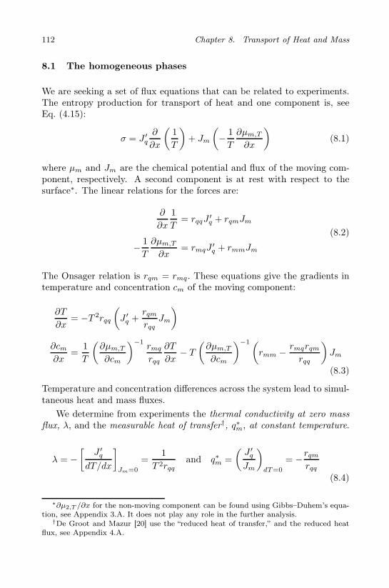
112 Chapter 8. Transport of Heat and Mass
8.1 The homogeneous phases
We are seeking a set of flux equations that can be related to experiments.The entropy production for transport of heat and one component is, seeEq. (4.15):
σ = J ′q
∂
∂x
(1
T
)+ Jm
(− 1
T
∂µm,T
∂x
)(8.1)
where µm and Jm are the chemical potential and flux of the moving com-ponent, respectively. A second component is at rest with respect to thesurface∗. The linear relations for the forces are:
∂
∂x
1
T= rqqJ
′q + rqmJm
− 1
T
∂µm,T
∂x= rmqJ
′q + rmmJm
(8.2)
The Onsager relation is rqm = rmq. These equations give the gradients intemperature and concentration cm of the moving component:
∂T
∂x= −T 2rqq
(J ′
q +rqm
rqqJm
)
∂cm∂x
=1
T
(∂µm,T
∂cm
)−1rmq
rqq
∂T
∂x− T
(∂µm,T
∂cm
)−1(rmm − rmqrqm
rqq
)Jm
(8.3)
Temperature and concentration differences across the system lead to simul-taneous heat and mass fluxes.
We determine from experiments the thermal conductivity at zero massflux, λ, and the measurable heat of transfer†, q∗m, at constant temperature.
λ = −[
J ′q
dT/dx
]
Jm=0
=1
T 2rqqand q∗m =
(J ′
q
Jm
)
dT=0
= −rqm
rqq
(8.4)
∗∂µ2,T /∂x for the non-moving component can be found using Gibbs–Duhem’s equa-tion, see Appendix 3.A. It does not play any role in the further analysis.
†De Groot and Mazur [20] use the “reduced heat of transfer,” and the reduced heatflux, see Appendix 4.A.

8.1. The homogeneous phases 113
The measured interdiffusion coefficient and thermal diffusion coefficient aredefined by:
Dm = −[
Jm
∂cm/∂x
]
dT=0
=1
T
∂µm,T
∂cm
(rmm − rmqrqm
rqq
)−1
=1
T
∂µm,T
∂cm
(rmm − rqq (q∗m)
2)−1
DT = −[
Jm
cm∂T/∂x
]
dcm=0
= −rmq/rqq
cmT 2
(rmm − rmqrqm
rqq
)−1
=q∗mcmT 2
(rmm − rqq (q∗m)
2)−1
(8.5)
With these coefficients, the gradients of the temperature and the concen-tration of the moving component become:
∂T
∂x= − 1
λ
(J ′
q − q∗mJm
)
∂cm∂x
= −cmDT
Dm
∂T
∂x− 1
DmJm
(8.6)
The relations Eq. (8.6), which are equivalent to the linear relations Eq. (8.2),contain transport coefficients which are known for many systems. The On-sager resistivity matrix can be found from such tabulated transport coeffi-cients using the following formulae:
rqq =1
λT 2, rqm = rmq = − q∗m
λT 2and rmm =
(q∗m)2
λT 2+
1
TDm
∂µm,T
∂cm
(8.7)
The Soret effect is mass transport that takes place due to a temperaturegradient. The ratio of the thermal diffusion coefficient and the interdiffu-sion coefficient is called the Soret coefficient, sT . In a stationary stateJm = 0, and the Soret coefficient can be determined from the ratio of theconcentration gradient and the temperature gradient:
sT = −(∂cm/∂x
cm∂T/∂x
)
Jm=0
=DT
Dm=
q∗mcmT
(∂µm,T
∂cm
)−1
(8.8)
We can alternatively measure the ratio of the heat flux and the molar fluxat constant temperature to find the heat of transfer q∗m, and then calculatethe Soret coefficient. Heat transport due to a concentration gradient is

114 Chapter 8. Transport of Heat and Mass
called the Dufour effect. This effect is the reciprocal effect to the Soreteffect. The Dufour coefficient is
DD = −(
J ′q
∂cm/∂x
)
dT=0
= q∗mDm = cmT∂µm,T
∂cmDT (8.9)
From the positive nature of the entropy production, it follows that the dif-fusion coefficient and the thermal conductivity are positive, cf. Eq. (7.21).The thermal diffusion coefficient, the measurable heat of transfer and theSoret coefficient can be positive or negative. From the inequality (7.22),using Eq. (8.7), we obtain
(rmq)2 ≤ rmmrqq →
(q∗mλT 2
)2
≤(
(q∗m)2
λT 2+
1
TDm
∂µm,T
∂cm
)1
λT 2
→ 0 ≤ ∂µm,T
∂cm(8.10)
The chemical potential will always increase when the concentrationincreases.
8.2 Coefficient values for homogeneous phases
Diffusion coefficients vary by orders of magnitude when one compares gases,liquids and solid phases, see Table 8.1. Within one phase, the variationis not so large for similar species. Diffusion coefficients are measured byspectroscopic and analytical techniques [70, 139,140].
Table 8.1 Examples of diffusion coefficients in binary mixtures Dm
Component m Reference component D/m2s−1
CH4 nitrogen gas 5× 10⁻⁵
NaCl water 1.3× 10⁻⁹
Sucrose water 4.5× 10⁻¹⁰
C steel 1× 10⁻²⁰
One can obtain an estimate for D from the self-diffusion coefficient,Ds, which is measured with NMR. The self-diffusion coefficient describesthe Brownian motion of a single particle at equilibrium, and can thereforealso be defined for pure components. The self-diffusion coefficient of water(in water) is 2.3 × 10⁻⁹ m2s−1 at 298 K [141].

8.2. Coefficient values for homogeneous phases 115
For gases, the kinetic theory gives Ds = ℓv/3, where ℓ is the meanfree path of the molecule and v is the mean thermal velocity. In a one-component gas ℓ =
(πa2cmN
)−1, where a is the diameter of the particles,
and v =√
3RT/M . With values ℓ = 30 nm and v = 300 ms−1 typical forair one finds Ds = 3× 10⁻⁶ m2s−1. This estimate can be compared to thediffusion coefficients for methane in nitrogen in Table 8.1. For low densitygas mixtures the diffusion and the self-diffusion coefficient are the same.For liquid mixtures they are not.
The Soret coefficient in gases is usually small. Nevertheless, the Soreteffect has been used to separate isotopes, a difficult separation. Isotopesdiffer by their masses only (m2 and m1). As a first approximation, Furryand Onsager [142] used
sT =0.35(m2 −m1)
T (m2 +m1)(8.11)
to describe a mass effect. This expression was used to design separationcolumns for radioactive isotopes. Isotope separation in salt mixtures wasmeasured by Lundén [143].
The interaction energy or the enthalpy is also important for the mag-nitude and sign of sT [144]. A formula for the thermal diffusion factor,α ≡ TsT , which has proven accurate for mixtures of two hydrocarbons,was proposed by Kempers [145].
αT ≡ − T
x1x2
∂x1
∂T= −
(V1V2
x1V1 + x2V2
)H1/V1 −H2/V2
x1(∂µ1/∂x1)p,T(8.12)
Here xi is the mole fraction, while Vi and Hi are the partial molar volumeand enthalpy, respectively. We return to this model in Sec. 12.5.
The Soret coefficient is often positive for the lighter component (negativefor the heavier component) as predicted from Eq. (8.11). Intermolecularinteractions may alter this. The Soret effect is larger in liquids than ingases, and the magnitude increases, the closer one comes to the criticalpoint [21]. A similar formula to Eq. (8.12) [21, 146] was used to predictcomposition variations with depth in oil reservoirs [147]. The variation wasequally large as the separation due to gravity for methane in decane [147].Some Soret coefficients for non-electrolytes are given in Table 8.2 [138].More data for electrolytes are given by Agar [148] and Fitts [30].
The effect of temperature gradients on mass transport can not only bedetermined by experiments, but also by molecular dynamics simulations,see Chapter 22, and Fig. 22.7 [149]. In these simulations a temperaturedifference is maintained over a box with two kinds of particles, by ther-mostatting the velocity of the molecules at the boundaries. The heavy

116 Chapter 8. Transport of Heat and Mass
Table 8.2 Soret coefficient for some binary mixtures. The mole fraction xm =cm/c applies to component m.
Component m Reference component xm T/K p/bar sT /K−1
Methane propane 0.34 346 60800 0.042Methane cyclopentane 0.0026 293 1 −0.016i-butane methylcyclopentane 0.5 293 1 −0.0096
Cyclohexane benzene 0.5 293 1 −0.0063Carbon dioxide hydrogen 0.51 223 15 0.00046
component concentrated on the cold side, and the light component on thewarm side. The consequence of the temperature difference was thus firsta mass flux, and eventually a concentration gradient. At stationary state,there were no longer mass fluxes relative to the walls.
Remark 8.1. In an experiment to measure the thermal conductivity, onestarts in an equilibrium state. This implies that the concentrations areconstant. After switching on a temperature gradient, one first measuresλm = −J ′
q/(∂T/∂x) = λ + q∗mcmDT . The temperature gradient proceedsto give a mass flux, which results after a while in a non-equilibrium dis-tribution of the concentration, such that the mass flux again becomes zero.In this stationary state one measures λ. This is why we will refer to λm
as the initial thermal conductivity and to λ as the stationary state thermalconductivity. The initial thermal conductivity is larger than the stationarystate thermal conductivity, because q∗mDT > 0.
Exercise 8.2.1. Express J ′q and Jm in terms of −T−2 (∂T/∂x) and
−T−1∂µm,T/∂x.
• Solution: By inverting Eqs. (8.2) we have:
J ′q = lqq
(− 1
T 2
∂T
∂x
)+ lqm
(− 1
T
∂µm,T
∂x
)
and
Jm = lmq
(− 1
T 2
∂T
∂x
)+ lmm
(− 1
T
∂µm,T
∂x
)
with
lqq =rmm
rqqrmm − rmqrqm, lmq = lqm =
−rqm
rqqrmm − rmqrqm,
lmm =rqq
rqqrmm − rmqrqm

8.3. The surface 117
Figure 8.1 The stationary state temperature profile across a room and adouble window in the absence of convection.
Exercise 8.2.2. Consider a room with air and a trace (10 ppm) of perfume,see Fig. 8.1. Near the wall, the temperature is 20 C (x = 0). Near thewindow at a distance of 4 m, the temperature is 10 C. One may use idealsolution conditions. The measurable heat of transfer of perfume in air isq∗m = 700 J/mol. The thermal conductivity is constant. Calculate theconcentration difference of perfume between the window and the wall in thestationary state. The room has heat leakage to one side only, as illustratedin the figure.
• Solution: In the stationary state there is no perfume flux. Thisimplies that, cf. Eq. (8.8),
dcmdx
= −cmsTdT
dx= − q∗m
T∂µm,T/∂cm
dT
dx= −cmq
∗m
RT 2
dT
dx
The heat flux is constant so that T (x) = 20−2.5x and a similar expres-sion for the molar density profile. This gives a temperature gradientof −2.5 K/m. The concentration gradient is therefore approximatelydcm/dx = 7000 (8.31)−1 (300)−2 2.5 ≃ 0.025 ppm/m. This gives aconcentration of 0.1 ppm higher at the window than close to the wall.Perfume concentrates at the cold side, it is heavier than air.
8.3 The surface
Consider next two homogeneous phases like the one described above, sepa-rated by an interface. The phase at x < 0 is labeled with superscript i, andthe phase at x > 0 is labeled with superscript o. The excess entropy pro-duction for the transport of heat and mass across the surface is, accordingto Eq. (5.15):

118 Chapter 8. Transport of Heat and Mass
σs = J ′iq ∆i,s
1
T+ J ′o
q ∆s,o1
T+ J i
m
(− 1
T s∆i,sµm,T (T s)
)
+ Jom
(− 1
T s∆s,oµm,T (T s)
)(8.13)
The notation of the forces was illustrated in Fig. 5.5. The force-flux pairsin the excess entropy production may be divided into two groups. The firstgroup contains coupling of fluxes and forces on the incoming side of thesurface and the second group contains coupling of fluxes and forces on theoutgoing side. Because the processes on the two sides of the surface occurin series, it is expected that they are weakly coupled. We shall thereforeneglect coupling across the surface. In that case, the force-flux relationsbecome
∆i,s1
T= rs,iqqJ
′iq + rs,iqmJ
im
− 1
T s∆i,sµm,T (T s) = rs,imqJ
′iq + rs,immJ
im
(8.14)
for side i of the surface and
∆s,o1
T= rs,oqq J
′oq + rs,oqmJ
om
− 1
T s∆s,oµm,T (T s) = rs,omqJ
′oq + rs,ommJ
om
(8.15)
for side o. All coefficients have the dimensionality of the resistivity co-efficients for the homogeneous phase, see Eqs. (8.2), times a length (thesurface thickness). All resistivity coefficients have superscript s to indicatethe surface. The next superscript gives the side of the surface for which theforce is evaluated. The number of independent resistivities is six.
Remark 8.2. The force-flux relations for the surface serve as boundaryconditions for integrations of temperature and chemical potential across ad-jacent bulk phases.
The measurable heats of transfer can be defined in a similar manner asfor the homogeneous system:
q∗im (T s) =
(J ′i
q
J im
)
∆i,sT=0
= −rs,iqm (T s)
rs,iqq (T s)
and q∗om (T s) =
(J ′o
q
Jom
)
∆s,oT=0
= −rs,oqm (T s)
rs,oqq (T s)(8.16)

8.3. The surface 119
With these definitions, Eqs. (8.14) and (8.15) can be written as
∆i,s1
T= rs,iqq
(J ′i
q − q∗imJim
)
1
T s∆i,sµm,T (T s) = rs,iqqq
∗imJ
′iq − rs,immJ
im
(8.17)
for side i of the surface and
∆s,o1
T= rs,oqq
(J ′o
q − q∗om Jom
)
1
T s∆s,oµm,T (T s) = rs,oqq q
∗om J ′o
q − rs,ommJom
(8.18)
for side o. The measurable heats of transfer are ratios of fluxes in thehomogeneous phases, so their values at the surface are equal to the valuesin the homogeneous phases next to the surface. The only new coefficients,that are needed to describe transport through the surface, are then the fourdiagonal coefficients in Eqs. (8.14) and (8.15).
8.3.1 Heats of transfer for the surface
The description in the beginning of the section uses the temperature of thesurface as a variable. We can eliminate T s for stationary state conditions,when the total heat flux Jq = J ′i
q +H imJ
im = J ′o
q +HomJ
om, and the molar
flux Jm = J im = Jo
m are constant. The jumps across the surface of theinverse temperature and the chemical potential, become with the additionof Eqs. (8.17) and (8.18):
∆i,o1
T=rs,iqq
(J ′i
q −q∗imJm
)+rs,oqq
(J ′o
q −q∗om Jm
)
=(rs,iqq +rs,oqq
)J ′i
q −[rs,iqqq
∗im+rs,oqq (q∗om +∆i,oHm)
]Jm
1
T s∆i,oµm,T (T s)=rs,iqqq
∗imJ
′iq −rs,immJm+rs,oqq q
∗om J ′o
q −rs,ommJm
=(rs,iqqq
∗im+rs,oqq q
∗om
)J ′i
q −(rs,imm+rs,omm+rs,oqq q
∗om ∆i,oHm
)Jm
(8.19)The matrix of coefficients is no longer symmetric. The reason for thisis that we have eliminated J ′o
q without making a corresponding changein the forces. This can be done by using ∆i,oµm,T (T o) /T o instead of∆i,oµm,T (T s) /T s. To simplify, we now replace superscript o,i of T by oonly. The difference is
1
T s∆i,oµm,T (T s) =
1
T o∆i,oµm,T (T o) − ∆i,oHm∆s,o
1
T(8.20)
120 Chapter 8. Transport of Heat and Mass
By introducing this into Eq. (8.19), we find:
∆i,o1
T= rsqqJ
′iq + rs,lqmJm
− 1
T o∆i,oµm,T (T o) = rs,lmqJ
′iq + rs,lmmJm
(8.21)
where
rsqq ≡ rs,iqq + rs,oqq , rs,lqm = rs,lmq ≡ −rs,iqqq∗i − rs,oqq (q∗om + ∆i,oHm)
rs,lmm ≡ rs,imm + rs,omm + rs,oqq ∆i,oHm (2q∗om + ∆i,oHm)(8.22)
The heat of transfer for the whole surface, derived from the measurable heatflux at the left hand side of the surface can then be defined as
q∗s,im =
(J ′i
q
Jm
)
∆i,oT=0
= −rs,lqm
rsqq
=rs,iqqq
∗im + rs,oqq (q∗om + ∆i,oHm)
rs,iqq + rs,oqq
(8.23)
As is clear from this relation q∗s,im is unequal to q∗im. In this context, ∆i,oT =0 does not mean that ∆i,sT = 0. Using the measurable heat of transfer,Eq. (8.21) becomes
∆i,oT = T iT orsqq
(J ′i
q − q∗s,im Jm
)
− 1
T o∆i,oµm,T (T o) = − q∗s,im
T iT o∆i,oT +
(rs,lmm − rsqqq
∗s,im q∗s,im
)Jm
(8.24)
It is also possible to eliminate the measurable heat flux on the left handside of the surface in Eq. (8.19). Instead of Eq. (8.21) we then obtain
∆i,o1
T= rsqqJ
′oq + rs,rqmJm
− 1
T i∆i,oµm,T
(T i)
= rs,rmqJ′oq + rs,rmmJm
(8.25)
where
rsqq ≡ rs,iqq + rs,oqq , rs,rqm = rs,rmq ≡ −rs,iqq
(q∗im − ∆i,oHm
)− rs,oqq q
∗om
rs,rmm ≡ rs,imm + rs,omm − rs,iqq∆i,oHm
(2q∗im − ∆i,oHm
) (8.26)
For the heat of transfer for the whole surface, derived from the measurableheat flux at the right hand side of the surface we find
q∗s,om =
(J ′o
q
Jm
)
∆i,oT=0
= −rs,rqm
rsqq
=rs,iqq
(q∗im − ∆i,oHm
)+ rs,oqq q
∗om
rs,iqq + rs,oqq
(8.27)

8.3. The surface 121
Equation (8.25) in terms of the measurable heat of transfer, becomes
∆i,oT = T iT orsqq
(J ′o
q − q∗s,om Jm
)
− 1
T i∆i,oµm,T
(T i)
= − q∗s,om
T iT o∆i,oT +
(rs,rmm − rsqqq
∗s,om q∗s,om
)Jm
(8.28)
An interesting identity which follows from Eqs. (8.23) and (8.27) is
q∗s,om − q∗s,im = −∆i,oHm (8.29)
This shows that the difference of the measurable heats of transfer that canbe defined for the whole surface, is equal to the enthalpy difference acrossthe surface. The rather common practice to take the coupling coefficientequal to zero, suggested by the small q∗im and q∗om , is therefore in violationwith this identity [61]. Given the fact that the enthalpy difference across aphase boundary is normally substantial, this can give a serious error.
Remark 8.3. In a practical situation, only one of the equation sets,Eq. (8.21) or (8.25), is needed to describe the transports at the surface.We shall see in Sec. 11.3 that one set has larger coefficients than the other,and may therefore be easier to determine.
Remark 8.4. In Sec. 12.2, we derive an equivalent relation, cf.Eq. (12.64), for the difference of the measurable heats of transfer acrossa finite film in a homogeneous phase. In that case, the enthalpy differencesare, however, much smaller. An interesting consequence of the validity ofboth these relations is that one may combine them and obtain the same re-lation for transport between two arbitrary planes between which there is asequence of homogeneous films with surfaces in between.
Exercise 8.3.1. Consider again the room with a trace of perfume from theprevious exercise. We want to take into account that perfume adsorbs tothe window. The perfume does not cross the window to disappear in theair outside. The temperature of the air just outside the window is −10 Cwhile the temperature in the room 4m away from the window, T il, is again20 C. How do the linear laws (8.17) and (8.18), which neglect the couplingresistances across the surface, simplify in a stationary state? The massfluxes are again zero. The thermal conductivity of air λ with perfume is0.01 W/Km, and the thermal resistivities for both sides of the window rs,iqq
and rs,oqq are 0.002 m2/WK. What is the resulting temperature profile andhow does this affect the perfume concentration difference?
• Solution: Since there is no perfume flux in the stationary state,J i = Jo = 0, the total heat flux is equal to the measurable heat

122 Chapter 8. Transport of Heat and Mass
flux. We know furthermore that the total heat flux and therefore themeasurable heat flux is constant throughout the system, J ′i
q = J ′oq =
J ′q. The force-flux equations become
∆i,s1
T= rs,iqqJ
′q and ∆s,o
1
T= rs,oqq J
′q
∆i,sµ
T= rs,iqqq
∗iJ ′q and ∆s,o
µ
T= rs,oqq q
∗oJ ′q
By adding the first two equations, we find 1/T o − 1/T i =(rs,iqq + rs,oqq
)J ′
q. As a consequence, T o − T i = −T oT i(rs,iqq + rs,oqq
)J ′
q =
−360J ′q. Furthermore, we know that in the room T i − T il =
−(4/λ)J ′q = −400J ′
q. The sum gives 30 = T il − T o = 760J ′q or
J ′q = 0.04 W/m2. The temperature difference across the room is
therefore T il − T i = 400 × 0.04 = 16C. In the previous exercise,the temperature difference was 10 degrees across the room, whichmade the concentration 0.10 ppm higher at the window. Now theperfume concentration is 0.16 ppm (60%) higher at the window. Thisexample shows that the surface can play a significant role.
Remark 8.5. The example is, of course, artificial in the sense that we donot allow the air to circulate. This would homogenize both the temperatureand the concentration. The surface above has a thickness of mm ratherthan nm. A surface does not have to be microscopically thick to qualify asa surface in the Gibbs sense. The only important condition is that the bulkregion adjacent to the surface is much thicker than the surface, and thatthe change of the temperature in the bulk over a distance comparable to thethickness of the surface is small, just as in the above exercise.
8.4 Solution for the heterogeneous system
For an analysis of the heterogeneous system, we write Eq. (8.2) after somealgebra in the following form
∂
∂x
1
T= rqq (Jq −Q∗
mJm)
∂
∂x
µm
T= rqqQ
∗mJq − [rmm +Hmrqq (2q∗m +Hm)] Jm
≡ rqqQ∗mJq − rµµJm (8.30)

8.4. Solution for the heterogeneous system 123
where we used J ′q = Jq −HmJm and the thermodynamic identity
∂µm/T
∂1/T= µm − T
∂µm
∂T= µm + TSm = Hm (8.31)
Furthermore, we defined the total heat of transfer by:
Q∗m =
(Jq
Jm
)
dT=0
=
(J ′
q +HmJm
Jm
)
dT=0
= q∗m +Hm = −rqm
rqq+Hm
(8.32)
and defined the resistivity rµµ in the last equality in Eq. (8.30).In the stationary state, energy and molar densities are independent of
time. As a consequence the total heat flux, Jq, and the component flux,Jm, are constant, both as a function of time and position. This makesEq. (8.30) suitable for integration. The measurable heat flux is not constantas a function of position due to the variation of the enthalpy density as afunction of the local temperature and the concentrations.
For the surface, we obtain in a similar manner from Eqs. (8.14) and(8.15)
∆i,s1
T= rs,iqq
[Jq −
(q∗im +H i
m
)Jm
]= rs,iqq
(Jq −Q∗i
mJm
)
∆i,sµm
T= rs,iqq
(q∗im +H i
m
)Jq −
[rs,imm + rs,iqqH
im
(2q∗im +H i
m
)]Jm
= rs,iqqQ∗iJq − rs,iµµJm (8.33)
for side i of the surface and
∆s,o1
T= rs,oqq [Jq − (q∗om +Ho
m)Jm] = rs,oqq (Jq −Q∗omJm)
∆s,oµm
T= rs,oqq (q∗om +Ho
m)Jq −[rs,omm + rs,oqq H
om (2q∗om +Ho
m)]Jm
= rs,oqq Q∗oJq − rs,oµµJm (8.34)
for side o. The coefficients rs,iµµ and rs,oµµ are defined in the last identities.We are now set to solve the temperature and concentration profiles
across a heterogeneous system. Consider therefore two homogeneous phaseswith an interface between them. The zero along the x-axis is chosen tocoincide with the position of the dividing surface. The left homogeneousphase is between −din and 0 and the right homogeneous phase is between0 and dout. The system is in a stationary state, so that the total heat

124 Chapter 8. Transport of Heat and Mass
flux, Jq, and the mass flux, Jm, are constant throughout the system. Thetemperatures at the ends are Tin = T (−din) and Tout = T (dout), and thechemical potentials are µin = µm(−din) and µout = µm(dout). In order tosimplify the calculation, we assume that the resistivities and the enthalpies(and as a consequence the heats of transfer) are constant. It then followsfrom Eq. (8.30) that the gradients of 1/T and µ/T in the two homogeneousphases are constant. By integrating these equations over the homogeneousphases, we find:
1
Tout− 1
Tin=
(1
Tout− 1
T o
)+
(1
T o− 1
T s
)
+
(1
T s− 1
T i
)+
(1
T i− 1
Tin
)
=(doutr
oqq + rs,oqq + rs,iqq + dinr
iqq
)Jq
−[(doutr
oqq + rs,oqq
)Q∗o
m +(rs,iqq + dinr
iqq
)Q∗i
m
]Jm
µout
Tout− µin
Tin=
(µout
Tout− µo
m
T o
)+
(µo
m
T o− µs
m
T s
)
+
(µs
m
T s− µi
m
T i
)+
(µi
m
T i− µin
Tin
)
=[(doutr
oqq + rs,oqq
)Q∗o
m +(rs,iqq + dinr
iqq
)Q∗i
m
]Jq
−(doutr
oµµ + rs,oµµ + rs,iµµ + dinr
iµµ
)Jm (8.35)
These equations make it possible to calculate Tout and µout given Tin, µin,Jq and Jm, or alternatively Jq and Jm given Tin, µin, Tout and µout. Ingeneral, four of these quantities make it possible to calculate the two others.Once the six quantities are known, it follows for the inverse temperaturethat
1
T (x)=
1
Tin+ (x+ din) riqq
(Jq −Q∗i
mJm
)for − din < x < 0
1
T s=
1
Tin+(dinr
iqq + rs,iqq
) (Jq −Q∗i
mJm
)
1
T (x)=
1
Tout+ (x− dout) r
oqq (Jq −Q∗o
mJm) for 0 < x < dout
(8.36)

8.5. Scaling relations between surface and bulk resistivities 125
For µm/T we find similarly that
µm(x)
T (x)=µin
Tin+ (x+ din)
(riqqQ
∗imJq − riµµJm
)for − din < x < 0
µsm
T s=µin
Tin+(dinr
iqq + rs,iqq
)Q∗i
mJq −(dinr
iµµ + rs,iµµ
)Jm
µm(x)
T (x)=µout
Tout+ (x− dout)
(roqqQ
∗omJq − roµµJm
)for 0 < x < dout
(8.37)
Equations (8.36) and (8.37) give the temperature and the chemical potentialprofiles through the system.
The above calculation, taking some quantities constant, should be seenas an illustration. For temperature dependent coefficients Eq. (8.30) mustbe integrated numerically to obtain the temperature and the chemical po-tential profiles in the homogeneous phases.
The Soret (or Dufour) effect is not a big effect in gases or liquids. It cantherefore often be neglected in descriptions of transport in homogeneoussystems. When it comes to heterogeneous systems this picture changesdramatically. The coupling coefficients for interface transports, here repre-sented by rs,iqqQ
∗im and rs,oqq Q
∗om , are large, as follows from Eq. (8.29). These
terms are the origin of the power that can be created in a thermal osmosisplant, see Chapter 18.
It has been verified that the temperature of a catalytic surface can bedifferent from that of the adjacent homogeneous phases [125, 150,151].
8.5 Scaling relations between surface and bulk resistivities
In order to compare surface and bulk main resistivities, we divide theirratio by the thickness of the surface, δ. A dimensionless scaling coefficientis obtained‡. For the left hand side of the surface, this gives:
ki =rs,i
riδ(8.38)
Such a ratio can be defined for the surface main resistivities. The Onsagercoefficient that describes the thermal resistivity for side i of the surface can,using such a scaling coefficient, be written as
rs,iqq = kiqδr
iqq =
kiqδ
λi (T i)2 (8.39)
‡Hansen [152] does this for the conductivities rather than for the resistivities. It isbetter to do this for the resistivities, as the resistivities are in series.

126 Chapter 8. Transport of Heat and Mass
where λi is the thermal conductivity and T i is the temperature of the bulkmaterial on side i. The mass transfer coefficient for side i, is similarly (forsystems with constant activity):
rs,iµµ = kiµδr
iµµ = ki
µδDici
RT i(8.40)
Similar expressions may be written down for the other side of the sur-face. The scaling coefficients measure how surface resistivities differ frombulk resistivities. The surface is only interesting as a separate system if ithas a substantial resistivity to transport, that is, when ki is substantiallylarger than unity. When ki is of the order unity or smaller, one may ig-nore the surface resistivity. In the above formulae, it is the product kiδrather than the scaling coefficient that has a physical significance. Thereis some freedom in the choice for the thickness of the surface δ but notin the product. For many heterogeneous systems, the transition from onehomogeneous phase to the other is very abrupt. For the interface betweenthem, a thickness of 1.5 times the diameter of the molecules is commonlyused [93]. In Chapter 22 we will discuss how to define a thickness for avapor-liquid interface appropriate for the interpretation of the results ofmolecular dynamics simulations [39].

Chapter 9
Transport of Heat and Charge
We present flux equations for transport of heat and charge, with the aimto be able to integrate across heterogeneous systems. We give the Onsagercoefficients in terms of the measured coefficients and discuss some coeffi-cient models. We show how thermal energy can be used to produce electricpower.
This chapter concerns transports of heat and charge. Coupling oc-curs between such transports in many solid state electrochemical systems,e.g. batteries and fuel cells. The coupling is important because it is theorigin of work in these systems. It is the only way in which one can pro-duce work from low temperature heat reservoirs; in thermoelectric powergenerators. Thermoelectric effects have been known since the 19th century.Seebeck found in 1821 that heating of one junction of a bimetalic coupleand cooling another gave rise to an electromotive force in the circuit. Thir-teen years later Peltier found that passage of an electric current through abimetalic circuit caused adsorption of heat. The coupling between trans-port of heat and charge explains the function of the common thermocoupleand thermoelectric heat pumps [153]. Such devices consist of two or moreconductors or semiconductors.
We give the basic equations for such transports across two homogeneousconductors, joined together by a surface. More complicated examples aregiven in Chapters 13–21. The electric current density is constant throughthe system, and we have no mass flux.
The aim is to give equations that can be integrated through the hetero-geneous system, to obtain the performance of the total system. The surfaceis always the frame of reference for the transport processes. Experimentalor other conditions determine the entropy production of the surface and ofthe homogeneous phases.
127

128 Chapter 9. Transport of Heat and Charge
9.1 The homogeneous phases
Consider an electric conductor. The temperature changes as a functionof position and so does the electric potential. By convention, the elec-tric current from left to right is positive. The entropy production for thehomogeneous phase is obtained from Eq. (4.15), which here reduces to:
σ = J ′q
(d
dx
1
T
)+ j
(− 1
T
dφ
dx
)(9.1)
The resulting equations for the forces are
d
dx
1
T= rqqJ
′q + rqφj
− 1
T
dφ
dx= rφqJ
′q + rφφj
(9.2)
These coefficients can be identified with coefficients that are obtained frommeasurements. Measurements define the stationary state thermal conduc-tivity (Fourier’s law):
λ ≡ −(
J ′q
dT/dx
)
j=0
=1
T 2rqq(9.3)
and the Ohm’s law resistivity
r ≡ −(dφ/dx
j
)
dT=0
= T
(rφφ − rqφrφq
rqq
)(9.4)
The Peltier coefficient, π, is the heat transferred reversibly with the electriccurrent (cf. remark under Eq. 7.25)
π ≡(J ′
q
j/F
)
dT=0
= −F rqφ
rqq(9.5)
Neither J ′q nor j depend on the frame of reference, so π is absolute. Be-
cause the Peltier coefficient concerns reversible heat transport, it has beenassociated with an entropy, the transported entropy of the charge carrier :
π ≡ TS∗ (9.6)
Here S∗ is the transported entropy of the charge carrier. We can expressthe resistivities in terms of the transport coefficients found from experimentas
rqq =1
T 2λ, rqφ = rφq = − π
FT 2λ, rφφ =
1
T
(r +
π2
F 2Tλ
)(9.7)

9.1. The homogeneous phases 129
By introducing these expressions into Eq. (9.2), the gradients in T andφ become
dT
dx= −
J ′q
λ+π
λ
j
F
dφ
dx= −S
∗
F
dT
dx− rj
(9.8)
The Onsager relation rqφ = rφq was used. By convention, the transportedentropy is positive when entropy is transported in the direction of the posi-tive electric current. Transported entropies are kinetic, not thermodynamicproperties. Electronic conductors have transported entropies between −1and −20 J/K mol [154]. Some transition metals like Mo, Cr and W havepositive transported entropies, even if the charge carrier is an electron. Themaximum value in molybdenum is S∗
e−,Mo = 17 J/K mol at 900 K [154]. Forthe same temperature, S∗
e−,Pb = −5 J/K mol. The transported entropy ofelectrons in lead is a commonly used reference value. The variation in thetransported entropy was to some extent explained by the number of elec-trons available for transport above the Fermi energy level (εF) at a giventemperature. Mott and Wilson, see Cahn [155], proposed that
S∗ =π
3
k2BT
eκ
[dκ
dεF
]
εF
(9.9)
Here κ is the specific electric conductivity, e is the absolute charge of theelectron, kB is Boltzmann’s constant and π is the mathematical constant.The derivative is taken at the value of the Fermi energy level, εF.
The transported entropy is a function of the temperature. This is de-scribed by the Thomson coefficient:
τ ≡ Td
dT
( πT
)= T
dS∗
dT(9.10)
If the transported entropy is zero at 0 K, we can find the transportedentropy at any temperature by integrating τ from 0 K to T .
S∗ =
∫ T
0
τ
TdT =
π(T )
T(9.11)
The result gives an absolute value for π(T )/T for a material. The Thomsonheat [7] is the heat added to a conductor to keep its temperature constantper faraday of positive charges passing the conductor from left to right.
Exercise 9.1.1. Consider an electric current of 10A/m2 through a pieceof lead. Entropy will be transported, and if the system is thermally isolated,
130 Chapter 9. Transport of Heat and Charge
a temperature gradient will build up. Calculate the maximum temperaturegradient that arise in the metal. Use a thermal conductivity of 5 W/Km andan average temperature of 300 K. The transported entropy is −5 J/K mol.
• Solution: Eq. (9.8) gives the heat flux in terms of the temperaturegradient and the electric current
J ′q = −λPb
dT
dx+ πPb
j
F
With a constant electric current, the heat flux through the systemwill vary (the variation is given by the energy balance for the isolatedmetal). The smallest value of the heat flux is zero. In that caseall thermal energy is converted to work (electric energy). It followsthen that dT/dx = πPbj/FλPb. By substituting the values of allcoefficients we obtain dT/dx = −3 × 10⁻² K/m.
9.2 The surface
Consider next the surface between the two phases, i and o. The excessentropy production of Eq. (5.15) reduces to
σs = J ′iq ∆i,s
1
T+ J ′o
q ∆s,o1
T+ j
(−∆i,oφ
T s
)(9.12)
There is one heat flux into the surface, J ′iq , and one heat flux out of the
surface, J ′oq , but j = ji = jo. We use the assumption that there is no
coupling between fluxes on different sides of the surface, cf. Sec. 8.4. Theforces become:
∆i,s1
T= rs,iqqJ
′iq + rsiφj
∆s,o1
T= rs,oqq J
′oq + rsoφj
− 1
T s∆i,oφ = rsφiJ
′iq + rsφoJ
′oq + rsφφj
(9.13)
These expressions are analogous to Eqs. (8.14) and (8.15) with a constantmass flux. The Onsager relations are: rsiφ = rsφi and rsoφ = rsφo. Nota-tion is further illustrated in Fig. 9.1. Each resistivity is a function of thetemperature of the surface. The definitions of the Fourier type thermalconductivities for the two sides are:
λs,i ≡ −(
J ′iq
∆i,sT
)
j=0
=1
T iT srs,iqq
and λs,o ≡ −(
J ′oq
∆s,oT
)
j=0
=1
T sT ors,oqq
(9.14)

9.2. The surface 131
i os
i,s s,o
i,o o,i
i,o
Figure 9.1 Standard notation used for transport across surfaces.
The Peltier coefficients are defined in the same manner as for the homoge-neous phases:
πi(T s) ≡(J ′i
q
j/F
)
∆i,sT=0
= −Frsiφ(T s)
rs,iqq(T s)
and πo(T s) ≡(J ′o
q
j/F
)
∆s,oT=0
= −Frsoφ(T s)
rs,oqq (T s)(9.15)
These coefficients are ratios of fluxes in the homogeneous phases and aretherefore equal to the corresponding values in these homogeneous phasesat the temperature of the surface. The ohmic resistivity of the surface is:
rs ≡ −(
∆i,oφ
j
)
T i=T s=T o
= T s
(rsφφ −
rsφirsiφ
rs,iqq
−rsφor
soφ
rs,oqq
)(9.16)
The resistivities can be expressed in the transport coefficients just definedas:

132 Chapter 9. Transport of Heat and Charge
rs,iqq =1
T iT sλs,iand rs,oqq =
1
T sT oλs,o
rsiφ = rsφi = − πi
FT iT sλs,iand rsoφ = rsφo = − πo
T sT oλs,o
rsφφ =1
T s
[rs +
(πi
F
)21
T iλs,i+
(πo
F
)21
T oλs,o
](9.17)
The jumps in the intensive variables into and across the surface are:
∆i,sT = T s − T i = − 1
λs,i
(J ′i
q − πi j
F
)
∆s,oT = T o − T s = − 1
λs,o
(J ′o
q − πo j
F
)
∆i,oφ = φo − φi = − 1
FS∗
i ∆i,sT − 1
FS∗
o∆s,oT − rsj
(9.18)
When the surface temperature differs from the temperatures in the adjacentphases, finite contributions to the cell potential result.
9.3 Thermoelectric coolers
The Peltier heat is defined for junctions [27]. The Peltier heat of a surface(the junction) is defined by the heat needed to keep the surface at constanttemperature when one faraday of positive charges is passing it from left toright:
πs (T s) ≡ −(J ′i
q − J ′oq
j/F
)
T i=T s=T o
= πo (T s) − πi (T s) (9.19)
The Peltier heat of a surface is the difference between the Peltier coeffi-cients in the two conductors, πo − πi. The Peltier effect is used to makecoolers, like for instance wine coolers. In a thermoelectric cooler, an electriccurrent is used to transport heat from a low temperature reservoir to a hightemperature reservoir.
Let us calculate the electricity needed to cool a glass of wine (25 cm3)at 300 K by 5 K, using a Mo–Pb element with the values for S∗ given inSec. 9.1. The heat capacity of wine (water) is 72 J/K mol. The Peltierheat of the device is πo − πi = [17− (−5)] 300 J/mol = 6.6 kJ/mol. There

9.4. Thermoelectric generators 133
are 25 · 10−3 · 55.5 = 0.14 mol water in the glass. The number of joulesneeded for cooling is taken from the junction of the element 0.14 · 72 · 5 =6.6 kJ/mol · Q/F , where Q is the number of coulombs and F is Faraday’sconstant. The relation demands 760 C, or 0.84 A in 900 s.
The reciprocal effect of the Peltier effect, the Seebeck effect, can be usedto generate electric power from geothermal and other heat sources. In thatcase a temperature difference exists (see below). It is easier to measure anelectric potential with high precision than a heat effect at zero temperaturerise. The Seebeck coefficient can therefore be more accurately determined,and can be used to determine the Peltier coefficient via Onsager’s reciprocalrelations, see for instance Flem and coworkers [78, 80].
9.4 Thermoelectric generators
A thermoelectric generator takes advantage of the heat flux between a highand a low temperature reservoir to generate electric power. The genera-tor consists of a p- and an n-semiconductor in series. Their junction iskept at the low temperature TL, while the other ends (the terminals) havetemperature TH . The system is illustrated in Fig. 9.2. An electric cur-rent is produced, and a potential can be measured between the terminals.The distance between the thermal reservoirs through both the p- and ann-semiconductor, l, is small, usually only a few mm. The geometry of thesystem is such that x = 0 at the terminal and x = l at the cold end in thep-semiconductor (phase i). The n-semiconductor (phase o) bends back andgoes from x = l at the cold end to x = 0 at the terminal, parallel to thep-semiconductor.
The electric potential of the generator is obtained by integrating fromterminal to terminal:
∆φ =
∫ l
0
(−S
∗i
F
dT
dx− rij
)dx+ ∆i,oφ+
∫ 0
l
(−S
∗o
F
dT
dx− roj
)dx (9.20)
Combining the integrals, taking T i = T s = T o, we obtain:
∆φ =
∫ l
0
[−ηS
dT
dx−(ri + ro
)j
]dx− rsj (9.21)
where ηS is the Seebeck coefficient of the device:
ηS =∆φ
(TH − TL)
∣∣∣∣j=0
=1
F(S∗
i − S∗o ) (9.22)
where we took the transported entropies independent of the temperatureto obtain the last identity. The electric potential difference is generated be-tween the terminals, because there is a difference in the transported entropy

134 Chapter 9. Transport of Heat and Charge
T
p nx
0
lTL
H
Figure 9.2 The thermo-electric generator composed of a p- and n-semiconductor, between thermal reservoirs with temperatures TH and TL.
of the charge carriers in the conductors. The maximum electric potentialis obtained when j = 0. The electric potential for j = 0 (the reversible po-tential) is given by the net heat added to the system from the surroundingsdivided by F (i.e. the first law applies for the total system). For a finite jthe potential becomes, using temperature independent electric resistivities,
∆φ = ηS(TH − TL) −(lri + rs + lro
)j ≡ ηS(TH − TL) − rtotalj (9.23)
The thermoelectric power
P ≡ j∆φ = ηS(TH − TL)j − rtotalj2 (9.24)
has a maximum Pmax = η2S(TH − TL)2/4rtotal as a function of the current
density. The current density delivered is determined by the resistance ofthe external circuit. Harman and Honig [153] gave the general expressionsfor temperature dependent transport coefficients.
Exercise 9.4.1. Calculate the Seebeck coefficient at 900 K for MoPbMoand find the maximum potential generated by a geothermal source of 90 oClying next to a glacier.
• Solution: By introducing the transported entropies given belowEq. (9.8), we find ηS = 21 µV/K. With ∆T = 90K,E = 180µVfor a single cell. By stacking many cells, one can generate a potentialdifference that supplies electric light to a nearby greenhouse.
Exercise 9.4.2. Find the entropy production in a thermoelectric generator.

9.5. Solution for the heterogeneous system 135
• Solution: The entropy production for one semiconductor (arm), saythe i-phase is:
σ = −(λi dT
dx+ S∗
i Tj
F
)dT
T 2dx−(−S
∗i
F
dT
dx− rij
)1
Tj
=λi
T 2
(dT
dx
)2
+1
Trij2
The reversible contributions to the entropy production containing S∗i
cancel. The entropy production for the whole device is
dSirr
dt= Ω
∫ l
0
(λ
T 2(dT
dx)2 +
1
Trj2)dx
where λ is the sum of the thermal conductivities of the homogeneousphases (the surface is isothermal) and Ω is the cross-sectional area.The terms in the entropy production are proportional to the squareof the gradient in temperature and the square of the current density.The entropy production times the temperature of the surroundingsgives the lost work per unit of time. The power is, on the other hand,a linear function of the temperature gradient. We therefore expect amaximum energy efficiency for a given temperature gradient.
We have seen that the examples in this chapter give relatively small effects.Still, the effect may be useful for dedicated purposes. The electric poten-tial created by a temperature difference is order of magnitude 1 mV, andrelatively much electricity is needed to provide cooling. The efficiency ofthese devices can be considerably improved if S∗ is raised. This gives amotivation to study thermogalvanic cells, see Chapters 13 and 14.
We have found that the main reason for energy conversion is the differ-ence in the transported entropies in the two phases. This is exploited indevices like coolers and generators. The larger the difference is, the largeris the efficiency of the device in its conversion of energy from one form toanother.
9.5 Solution for the heterogeneous system
In order to solve the heterogeneous system, it is convenient to use the fluxesthat are constant through the surface. These are the electric current j, andthe energy current Ju ≡ Jq + jφ = J ′
q + jφ. The entropy production in thehomogeneous phases in terms of these fluxes becomes (cf. Eq. (4.17)),
σ = Ju
(d
dx
1
T
)+ j
(− d
dx
φ
T
)(9.25)
136 Chapter 9. Transport of Heat and Charge
The resulting equations for the forces are
d
dx
1
T= reeJu + reφj
− d
dx
φ
T= rφeJu + re
φφj
(9.26)
By comparing with Eq. (9.2), we can identify
rqq = ree, rqφ = rφq = reφ + φree, rφφ = reφφ + 2φreφ + φ2ree (9.27)
Inverting these relations, we have
ree = rqq , reφ = rφe = rqφ − φrqq , reφφ = rφφ − 2φrqφ + φ2rqq (9.28)
where we used that both matrices, used in Eqs. (9.2) and (9.26), satisfy theOnsager symmetry relations.
The excess entropy production of the surface, Eq. (5.17), becomes
σs = Ju
(∆i,o
1
T
)+ j
(−∆i,o
φ
T
)(9.29)
where we used that J iu = Jo
u = Ju. The continuity of both fluxes throughthe surface results in the elimination of a force-flux pair of the surface. Asa consequence, the excess entropy production no longer depends on thetemperature differences with the surface. The forces become:
∆i,o1
T= rseeJu + rseφj
−∆i,oφ
T= rsφeJu + rs,eφφj
(9.30)
By calculating the same jumps, using the expressions for the forces (9.13),one can identify
rsee = rs,iqq + rs,oqq , rseφ = rsφe = rsiφ + rsoφ − φirs,iqq − φors,oqq
rs,eφφ = rsφφ − 2φirsiφ − 2φorsoφ +(φi)2rs,iqq + (φo)
2rs,oqq
(9.31)
These equations give the three coefficients used in Eq. (9.30) in terms ofthe five coefficients used in Eq. (9.13). It is therefore not possible to invertthis identification.

9.5. Solution for the heterogeneous system 137
We are now set to solve the temperature and electric potential pro-files across the heterogeneous system. Consider therefore two homogeneousphases with an interface between them. The zero along the x-axis is chosento coincide with the position of the dividing surface. The left homoge-neous phase is between −din and 0 and the right homogeneous phase isbetween 0 and dout. The temperatures at the ends are Tin = T (−din)and Tout = T (dout), and the electric potentials are φin = φ(−din) andφout = φ(dout). In order to simplify the calculation, we assume that theresistivities in both phases are independent of the position. It then followsfrom Eq. (9.26) that the gradients of 1/T and φ/T in the two homogeneousphases are constant. By integrating these equations over the homogeneousphases, using Eq. (9.30) for the surface, we find:
1
Tout− 1
Tin=
(1
Tout− 1
T o
)+
(1
T o− 1
T i
)+
(1
T i− 1
Tin
)
=(doutr
oee + rsee + dinr
iee
)Ju +
(doutr
oeφ + rseφ + dinr
ieφ
)j
φout
Tout− φin
Tin=
(φout
Tout− φo
T o
)+
(φo
T o− φi
T i
)+
(φi
T i− φin
Tin
)
= −(doutr
oeφ + rseφ + dinr
ieφ
)Ju −
(doutr
oφφ + rsφφ + dinr
iφφ
)j
(9.32)These equations make it possible to calculate Tout and φout given Tin, φin,Ju and j, or alternatively Ju and j given Tin, φin, Tout and φout. In general,four of these quantities make it possible to calculate the two others. Oncethe six quantities are known, it follows for the inverse temperature profilethat
1
T (x)=
1
Tin+ (x+ din)
(rieeJu + rieφj
)for − din < x < 0
1
T o=
1
Tin+ din
(rieeJu + rieφj
)
1
T i=
1
T o+ rseeJu + rseφj
1
T (x)=
1
T i+ x
(roeeJu + roeφj
)
=1
Tout+ (x− dout)
(roeeJu + roeφj
)for 0 < x < dout (9.33)

138 Chapter 9. Transport of Heat and Charge
For φ(x)/T (x), we similarly find
φ(x)
T (x)=φin
Tin− (x+ din)
(riφeJu + riφφj
)for − din < x < 0
φo
T o=φin
Tin− din
(riφeJu + riφφj
)
φi
T i=φs
T s− rsφeJu − rsφφj
φ(x)
T (x)=φi
T i− x
(roφeJu + roφφj
)
=φout
Tout− (x− dout)
(roφeJu + roφφj
)for 0 < x < dout (9.34)
Equations (9.33) and (9.34) give the temperature and electric potentialprofiles through the system. Given these profiles one can calculate the heatflux J ′
q(x) ≡ Ju−jφ(x) everywhere in the system. Equation (9.18) makes itthen possible to calculate the temperature of the surface. When riee, r
ieφ =
riφe, riφφ, roee, r
oeφ = roφe, r
oφφ depend on the temperature and/or the electric
potential, numerical integration is necessary to obtain the temperature andelectric potential profiles in the homogeneous phases.
By comparing Secs. 9.5 and 8.4, we see that Jq and Ju play comparableroles in the solution for the heterogeneous system. The two constant fluxesare practical for the integration procedure. After integration, we need toreintroduce J ′
q to be able to describe experiments or device performances.In order to find the terminal potential of a thermoelectric generator underoperation, and internal gradients of T (x) and φ(x), we replace Ju in theequations above by J ′
q + jφ.

Chapter 10
Transport of Mass and Charge
We give flux equations for transport of mass and charge in an electrochemi-cal cell. We give the Onsager coefficients in terms of measured coefficients,and present expressions for electrode potential jumps. We show how powerproduction is related to the coupling coefficients.
This chapter concerns mass and charge transports. Such transport oc-curs in electrochemical systems, e.g. electrolysis cells, batteries and fuelcells, but also in biological systems. The coupling between mass and chargetransport is frequently large, meaning that simple transport laws are inad-equate. In order to bring out the meaning of coupling, we consider againonly coupling of two fluxes with two forces. The aim is to give equationsthat can be integrated through the heterogeneous system, to obtain theperformance of the total system. We lay here a basis for the description ofsuch transports, building on Guggenheim, Førland et al. and Katchalskyand Curran [23, 27, 63]. The concentration overpotential, but not the acti-vation overpotential, is described. More complicated examples are given inChapters 13–21.
The cell used to illustrate the principles is the isothermal concentrationcell,
Ag (s) |AgNO3 (aq)|Ag (s) (10.1)
The electrodes are made of pure solid silver, which is a good electric con-ductor. The electric potential in both electrodes can therefore be takenconstant. On the left hand surface, we have oxidation of silver:
Ag → Ag+ + e− (10.2)
The electrolyte is AgNO3 in water, and there is a varying concentration ofthe salt across the cell. Silver ions go into solution from the anode surfaceand are deposited on the cathode surface as silver after the reverse reaction,
139

140 Chapter 10. Transport of Mass and Charge
Figure 10.1 An isothermal electrochemical cell with a concentrationgradient.
Ag+ + e− → Ag. Electric current is passing the cell from left to right. Inthe stationary state, both surfaces have the same velocity. All fluxes arecalculated with the surfaces as frame of reference. The velocity of the silverboth in the anode and the cathode relative to these surfaces is j/FcAg. Wecontinue to deal with one-dimensional transports through a heterogeneoussystem, in the direction normal to a flat surface, in the same manner asdescribed in Chapters 8 and 9. The fluxes at the surface not only have abearing on the form we choose for the entropy production at the surface,but also on the form chosen in the homogeneous phases.
In order to demonstrate the importance of coupling we consider twoexamples of coupled mass and charge transport, a salt power plant andelectric power from volume flow.
10.1 The electrolyte
Consider first the aqueous solution of AgNO3, see Fig. 10.1. The solutionis electroneutral, so the concentration of salt is equal to that of the cationand of the anion:
cAgNO3= cAg+ = cNO−
3
(10.3)
The mass balance for the salt is:
∂
∂tcAgNO3
(x, t) = − ∂
∂xJAgNO3
(x, t) (10.4)
so the two ions diffuse together.

10.1. The electrolyte 141
The entropy production, cf. Eq. (4.15) is:
σ = JAgNO3
(− 1
T
∂µAgNO3
∂x
)+ j
(− 1
T
∂φ
∂x
)(10.5)
The temperature is constant, so we drop subscript T for µAgNO3. Chemical
potentials for strong electrolytes were defined in Appendix 3.A.3. As willbe explained in Sec. 10.3, the electric potential φ is equal to ψ + µAg+/F ,where ψ is the electric potential referred to vacuum (the Maxwell potential).We shall use the φ-potential, because of its closer relation to measurablequantities. The force-flux relations are:
− 1
T
∂
∂xµAgNO3
= rµµJAgNO3+ rµφj
− 1
T
∂φ
∂x= rφµJAgNO3
+ rφφj
(10.6)
In the surface frame of reference, water is at rest. We define the experi-mental coefficients first. The diffusion coefficient, DAgNO3
, in Fick’s law isdefined when j = 0:
DAgNO3≡ −
(JAgNO3
∂cAgNO3/∂x
)
j=0
=1
Trµµ
∂µAgNO3
∂cAgNO3
(10.7)
The ohmic resistivity of the homogeneous solution is
re = −(∂φ/∂x
j
)
dµAgNO3=0
= T
(rφφ − rφµrµφ
rµµ
)(10.8)
and the transference coefficient of AgNO3 is the flux of salt divided by theelectric current density over F :
tAgNO3=
(JAgNO3
j/F
)
dµAgNO3=0
= −F rµφ
rµµ(10.9)
With these definitions, we can identify the resistivities in the force-fluxmatrix in terms of the measured transport coefficients by:
rµµ =1
TDAgNO3
∂µAgNO3
∂cAgNO3
, rµφ = rφµ = − tAgNO3
FTDAgNO3
∂µAgNO3
∂cAgNO3
rφφ =re
T+
(tAgNO3
F
)2 ∂µAgNO3/∂cAgNO3
TDAgNO3
(10.10)

142 Chapter 10. Transport of Mass and Charge
The concentration gradient and the electric force become, using themeasured transport coefficients:
∂cAgNO3
∂x= − JAgNO3
DAgNO3
+tAgNO3
DAgNO3
j
F
∂φ
∂x= − tAgNO3
F
∂µAgNO3
∂x− rej
(10.11)
The first term on the right hand side in Eq. (10.11b) gives the reversiblechemical work done by the system on expense of its internal energy. Thiscan be seen by introducing Eq. (10.6) into Eq. (10.5) and comparing com-pensating terms, see also Eq. (7.25). The transference coefficient can bedetermined by a Hittorf experiment [97]. In this experiment, an electriccurrent is passing a cell of a uniform composition. A differential amountof salt will accumulate on one of the sides, and can be taken for analysisto determine the number of moles transported per moles of electric chargethat is passing. The anode produces one mole of silver ion, and the cath-ode consumes one mole per faraday of electrons passing the outer circuit.These changes plus the transport in the electrolyte lead to a change incomposition on both sides. The total flux of silver nitrate is found fromEq. (10.11a). The equation says that, in order to find tAgNO3
, one mustcorrect for diffusion. This can be done by measuring the concentration gra-dient for small values of j for a decreasing period of time and extrapolatingto a zero period of time.
Equation (10.11b) can be used to find tAgNO3in the limit j → 0, when
the chemical potential is known at the two electrodes. The electric potentialdifference can be measured with high accuracy. This value may be moreaccurate than that obtained from Hittorf experiments.
The transport number of an ion is the fraction of the electric currentcarried by the ion:
tAg+ = F
(JAg+
j
)
dµAgNO3=0
and tNO−
3
= −F(JNO−
3
j
)
dµAgNO3=0
(10.12)
The two ions move in opposite directions, but together they are responsiblefor the total electric current, therefore
tAg+ + tNO−
3
= 1 (10.13)
The electrode surface reactions are here reversible to Ag+ ions on bothsides. The NO−
3 ions do not leave the electrolyte. The flux of the Ag+ ions
10.2. The electrode surfaces 143
is therefore equal to j/F plus the salt flux, while the flux of NO−3 ions is
equal to the salt flux alone:
JAg+ = j/F + JAgNO3and JNO−
3
= JAgNO3(10.14)
We obtain as a consequence
tAgNO3= −tNO−
3
(10.15)
The transference coefficient for salt can thus be expressed in two alternativeways:
tAgNO3= −tNO−
3
= −1 + tAg+ (10.16)
A model for transport numbers in terms of mobilities is discussed inSec. 10.6.
Remark 10.1. The transference coefficient for a salt in the electrolyte isdetermined by the transport number of the ion for which the reaction at theelectrode surfaces is reversible [27]. Transference coefficients are thereforenot a material property of the electrolyte alone. The transport numbers,however, are properties of the electrolyte.
10.2 The electrode surfaces
Consider again the electrode reaction
Ag → Ag+ + e− (10.17)
The surface dissolves as the reaction proceeds. This particular reaction isnormally in equilibrium, but for the example, we include its reaction Gibbsenergy. The excess entropy production of the isothermal anode surfacebecomes:
σs,a = Je,aAgNO3
(−∆s,eµAgNO3
T
)+ j
(−∆a,eφ+ ∆nG
s,a/F
T
)(10.18)
cf. Eq. (5.15). The Gibbs energy change of the neutral components is
∆nGs,a = −µa
Ag (10.19)
The silver phase on the left end is denoted a (from anode), the electrolytephase is denoted e. The terminology was further explained in Fig. 5.5. Theframe of reference, moving relative to the laboratory frame, is the equimolarsurface of silver. The electric current density is constant. The reaction rateis given by rs,a = j/F.

144 Chapter 10. Transport of Mass and Charge
The electric potential in the anode φa is equal to the Maxwell potentialminus the chemical potential of the electron divided by F , φa = ψa−µa
e−/F ,see also the Appendix 4.A and Sec. 10.7 [23, 27, 63]. In the electrolyte onesimilarly has φe = ψe + µe
Ag+/F . A reversible electrode has σs,a = 0,meaning that ∆s,eµAgNO3
= 0, and
∆a,eφ = φe − φa = −∆nGs,a
F→ ∆a,eψ = ψe − ψa = −∆rG
s,a
F(10.20)
where∆rG
s,a = µeAg+ + µa
e− − µaAg (10.21)
Equation (10.20) is the Nernst equation. The thermodynamic force is minus∆a,eφ + ∆nG
s,a/F = ∆a,eψ + ∆rGs,a/F divided by the temperature, see
Sec. 10.7.There are thus only two independent fluxes and forces:
−∆s,eµAgNO3
T= rs,aµµJ
e,aAgNO3
+ rs,aµφj
− 1
T
(∆a,eφ+
∆nGs,a
F
)= rs,aφµJ
e,aAgNO3
+ rs,aφφj
(10.22)
The adsorption coefficient for the motion of AgNO3 from the electrolyte toor from the surface is:
ℓs,aAgNO3≡ −
(Je,a
AgNO3
∆s,eµAgNO3
)
j=0
=1
rs,aµµT(10.23)
The stationary state ohmic resistivity of the surface becomes
rs,a ≡ −(
∆a,eφ+ ∆nGs,a/F
j
)
∆s,eµAgNO3=0
= T
(rs,aφφ −
rs,aφµrs,aµφ
rs,aµµ
)
(10.24)
The transference coefficient is the ratio of two bulk fluxes and is thereforeequal to the value in the electrolyte
teAgNO3≡(Je,a
AgNO3
j/F
)
∆s,oµAgNO3=0
= −Frs,aµφ
rs,aµµ= −te
NO−
3
(10.25)
With these definitions, we can identify the resistivities in the force-flux

10.2. The electrode surfaces 145
matrix in terms of the measured transport coefficients by:
rs,aµµ =1
T ℓs,aAgNO3
, rs,aµφ = rs,aφµ = −teAgNO3
FTℓs,aAgNO3
,
rs,aφφ =rs,a
T+
(teAgNO3
F
)21
T ℓs,aAgNO3
(10.26)
The chemical potential difference of AgNO3 out of the surface and thesurface potential drop become:
∆s,eµAgNO3= − 1
ℓs,aAgNO3
Je,aAgNO3
+teAgNO3
ℓs,aAgNO3
j
F
∆a,eφ+∆nG
s,a
F= −
teAgNO3
F∆s,eµAgNO3
− rs,aj
(10.27)
According to the last term of Eq. (10.27a) and Eq. (10.25), the electriccurrent transports salt in direction of the anode surface. This leads to anincrease in the salt concentration near the surface. The concentration canincrease until Je,a
AgNO3= 0. The chemical potential drop has then increased
to its maximum value. The driving force for desorption is then balancedby the migration of ions with the electric current.
The above analysis can be used in an analogous manner for the isother-mal cathode surface.
Exercise 10.2.1. Calculate the stationary state (Je,aAgNO3
= 0) chemicalpotential jump from the silver surface to the silver nitrate solution, for anelectric current density of 10 A/m2. The mobility coefficient of AgNO3 inand out of the surface is ℓs,aAgNO3
= 7.5 × 10⁻⁸ mol2/sJm2. The transportnumber for nitrate is te
NO−
3
= 0.6.
• Solution: Using Eq. (10.27a), one finds the chemical potential dif-ference equal to −jte
NO−
3
/Fℓs,aAgNO3. That gives a chemical potential
jump from the surface to the solution of −800 J/mol.
The jump in chemical potential gives a change in electric potential atthe surface, which is called the concentration overpotential, i.e. the changein the surface potential drop caused by lack of equilibrium between thesurface and the nearby electrolyte solution [156]. In order to describe theactivation overpotential [156], we need to consider the activated processon a mesoscopic level [51]. It is then possible to find the Butler–Volmerequation from σs. This is however outside the scope of this book.

146 Chapter 10. Transport of Mass and Charge
10.3 Solution for the heterogeneous system
The electrodes are good conductors and we can therefore take the electricpotentials φa and φc as constant. The chemical potential of the pure silverin both electrodes is the same on both sides at constant T and p, µa
Ag =µc
Ag. The origin of the x-axis is set at the silver-electrolyte interface. Thethickness of the electrolyte layer is de. The electric potential differenceacross the cell is
φc − φa = φc − φe,c + φe,c − φe,a + φe,a − φa
= ∆a,eφ+ ∆eφ+ ∆e,cφ
= − 1
FtAgNO3
(µs,c
AgNO3− µs,a
AgNO3
)− (rs,a + rede + rs,c) j (10.28)
For the last identity we integrated Eq. (10.11b), assuming that the transfer-ence number as well as the resistivity of the electrolyte are constant (takenat the average salt concentration). Furthermore we used Eq. (10.27) for theanode surface and the analogous equation for the cathode surface. Finally,we used µa
Ag = µcAg so that ∆nG
s,a + ∆nGs,c = 0, and ∆a,eφ+ ∆e,cφ = 0.
Assume next that rφφ and rµφ in the electrolyte are constant (dependonly on the average salt concentration). In the stationary state, the saltflux is zero. From Eqs. (10.6) and (10.22), we obtain the electric potentialdifference
φc − φa = −T(rs,aφφ + der
eφφ + rs,cφφ
)j (10.29)
and the chemical potential difference
µs,cAgNO3
− µs,aAgNO3
= µs,cAgNO3
− µe,cAgNO3
+ µe,cAgNO3
− µe,aAgNO3
+ µe,aAgNO3
− µs,aAgNO3
= ∆s,eµAgNO3+ ∆eµAgNO3
+ ∆e,sµAgNO3
= −T(rs,aµφ + der
eµφ + rs,cµφ
)j (10.30)
In this approximation, the chemical potential difference is linear in x andgiven by
µeAgNO3
(x) = 2µeAg+ (x) = 2µe
NO−
3
(x) = µeAgNO3
(0) − xTreµφ (10.31)

10.4. A salt power plant 147
Figure 10.2 The principle of a salt power plant that uses reverse electrodial-ysis. The concentration difference of sodium chloride, between the sea waterand the fresh water, drives an electric current and creates an electric power.Sodium ion is transported through cation exchange membranes, and chlorideions through anion exhange membranes.
10.4 A salt power plant
In order to see the importance of coupling coefficients for work production,consider first a salt power plant. This plant uses an electrolyte concentra-tion difference to give electric current. The plant that uses reverse electro-dialysis is illustrated in Fig. 10.2. Salt power plants can also use reverseosmosis, see Chapter 18. The plant operates at the sea level. Sea water andfresh water are fed into alternating compartments that are separated by ion-exchange membranes. The membranes alternate between cation exchangemembranes (A) and anion exchange membranes (C). One cell unit consistsof a salt water compartment, an anion exchange membrane, a fresh watercompartment, a cation exchange membrane and a salt water compartment.Several units in series add to the cell potential. The figure shows two units.The gradient in chemical potential of salt drives chloride ions through theanion-exchange membrane and sodium ions through the cation-exchangemembrane. The electric field that arises causes the electric current be-tween the electrodes. The chloride electrode, on the left hand side, may beof titanium oxide. On the right hand side, hydrogen rather than Na willbe produced, typically on a nickel electrode. We assume equilibrium at theelectrodes.
For each membrane, the electric potential difference is given by anexpression like Eq. (10.28). For the first membrane A in Fig. 10.2,

148 Chapter 10. Transport of Mass and Charge
tNaCl = tNa+ = 1.
∆φ = − tNa+
F[µNaCl (fresh) − µNaCl (sea)] − rmdmj (10.32)
where we took the electric resistance of the membrane, rmdm, to be largecompared to other resistances. The absolute value of the coupling coeffi-cient, |rµφ| = rµµtNa+/F , has its maximum when tNa+ = 1, see Eq. (10.9).Diffusion of salt reduces the electric power. Such a loss of power is pre-vented with this type of membrane arrangement. Eventually, there willbe some salt in the fresh water compartment to lower the chemical poten-tial difference. But some salt is also required to give an acceptable ohmicresistance in this compartment.
10.5 Electric power from volume flow
Work can also be obtained from volume transport between two pressurelevels. This transport can lead to charge transport in an outer circuit.Consider the transport of water across a cation exchange membrane in thecell
(Pt)H2,H2O(l)|HM|H2,H2O(l) (Pt) (10.33)
A platinum catalyst is located on the electrode-membrane interfaces. Themembrane HM is a proton conductor, for instance a Nafion membrane thatis used in fuel cells (see Chapter 19). The membrane needs water to conductwell. Hydrogen gas disproportionates on the left hand side giving protonsin the membrane and electrons in the metal. The protons react on theright hand side to form hydrogen gas. We assume now equilibrium at bothelectrodes. The entropy production of the membrane is, cf. Eq. (4.14):
σ = Jw
(− 1
T
∂µw
∂x
)+ j
(− 1
T
∂φ
∂x
)(10.34)
The proton concentration in the membrane is everywhere fixed by the cationsites of the membrane, so the flux of protons is identical to the electriccurrent j. The temperature is assumed to be constant so we drop thesubscript T in µw. The flux equations are:
Jw = −Lµµ1
T
∂
∂xµw − Lµφ
1
T
∂φ
∂x
j = −Lφµ1T
∂
∂xµw − Lφφ
1
T
∂φ
∂x
(10.35)
The frame of reference for transport are the membrane surfaces. In thisframe of reference, water can move due to a pressure difference between thetwo sides.

10.5. Electric power from volume flow 149
The electric conductivity of the membrane is
κe ≡ Lφφ
T(10.36)
Following the same procedure as in Secs. 10.1–10.3, we arrive at an expres-sion for the water flux
Jw = −Dw∂
∂xcw +
twFj (10.37)
where Dw is the diffusion coefficient of water in the membrane
Dw =
(Lµµ − LµφLφµ
Lφφ
)∂µw
∂cw(10.38)
while the transference coefficient of water is defined as:
tw = F
(Jw
j
)
dµw=0
= FLµφ
Lφφ(10.39)
When the water concentration is the same on the two sides, and ahydrostatic pressure difference exists, dµw = Vwdp, where Vw is the partialmolar volume of water. We solve Eq. (10.35) using Lφµ = Lµφ and obtain:
∆φ = −∫ de
0
(Lφµ
Lφφ
dµw
dx− j
κe)dx = − tw
F
∫ de
0
dµw−j
κede = − tw
FVw∆ep−
j
κede
(10.40)The pressure driven flow is able to generate an electric potential, however,this is small. This phenomenon is also called friction electricity. The mag-nitude of the work is proportional to tw or in other words, to the couplingcoefficient Lφµ.
The transference coefficient can be found by measuring the water fluxor the volume flow caused by electric current through the membrane, or bymeasuring the electric potential difference with different water pressures onthe two sides [157]. The relation between the two experiments is given bythe Onsager relation:
(∆eφ
∆ep
)
j=0
= −(Jw
j
)
dµw=0
= − twF
(10.41)
This is known as the Saxén relation. Volume flow by electric current is calledelectro-osmosis, while an electric potential generated by pressure differenceis called a streaming potential [27].

150 Chapter 10. Transport of Mass and Charge
10.6 Ionic mobility model for the electrolyte
In an electroneutral system, the independent composition variables are thesalt concentrations. The electrolyte can be regarded as electroneutral.Jackson [158] calculated that electroneutrality was obtained in a liquidjunction within 10−9 s, the time an ion takes to diffuse over a typical De-bije length. We are normally dealing with much larger time scales, compareExercise 7.2.2. It is still more common to use ions as basic variables forfluxes and forces. We shall therefore explain how to go from one descriptionto the other. This is useful for comparison with data in the literature.
The electrochemical potential for an ion was defined by Guggenheim[63,95].
µ+ = µ+ + z+Fψ
µ− = µ− − z−Fψ(10.42)
where µ+ and µ− are the chemical potentials for the cation and anionrespectively, ψ is the electrostatic potential referred to vacuum (the Maxwellpotential), and z+ and z− are ion valences (1 for both Ag+ and NO−
3 ).In the ionic formulation the entropy production is given by:
σ = JAg+
[− 1
T
∂
∂x
(µAg+ + Fψ
)]+ JNO−
3
[− 1
T
∂
∂x
(µNO−
3
− Fψ)]
(10.43)
By substituting JAg+ = j/F+JAgNO3, JAgNO3
= JNO−
3
and µNO−
3
+µAg+ =
µAgNO3, we see that this equation is equivalent to (10.5), given that
φ = ψ +µAg+
F(10.44)
The difference ∆φ is therefore equal to the electrochemical potential dif-ference divided by F of the ion that enters the electrode reaction, or the(measured) electromotive at reversible conditions [23, 27, 63]. The ionicfluxes, that follow from the entropy production (10.43), are:
JAg+ = −L++ 1
T
∂
∂x
(µAg+ + Fψ
)− L+− 1
T
∂
∂x
(µNO−
3
− Fψ)
JNO−
3
= −L−+ 1
T
∂
∂x
(µAg+ + Fψ
)− L−− 1
T
∂
∂x
(µNO−
3
− Fψ) (10.45)
In this formulation, Nernst–Einstein assumption holds for each ion. By

10.6. Ionic mobility model for the electrolyte 151
introducing measurable forces, we obtain:
JAg+ = −L+− 1
T
∂
∂xµAgNO3
− (L++ − L+−)F
T
∂φ
∂x
JNO−
3
= −L−− 1
T
∂
∂xµAgNO3
− (L−+ − L−−)F
T
∂φ
∂x
(10.46)
By expressing the salt flux and the electric current in terms of the ioniccoefficients, we obtain:
JAgNO3= −L−− 1
T
∂
∂xµAgNO3
− (L+− − L−−)F
T
∂φ
∂x
= −Lµµ1
T
∂
∂xµAgNO3
− Lµφ1
T
∂φ
∂x
j = −(L+− − L−−)F
T
∂
∂xµAgNO3
− (L++ − 2L+− + L−−)F 2
T
∂φ
∂x
= −Lφµ1
T
∂
∂xµAgNO3
− Lφφ1
T
∂φ
∂x(10.47)
which gives as relations for the conductivities in the salt representation:
Lµµ = L−−, Lµφ = Lφµ = (L+−−L−−)F, Lφφ = (L++−2L+−+L−−)F 2
(10.48)The conductivity matrix (Lµµ, Lµφ, Lφµ, Lφφ) is the inverse of the resistiv-ity matrix (rµµ, rµφ, rφµ, rφφ) in Eq. (10.6). In the ionic mobility model oneneglects L+− = L−+, which is of the second order in the salt concentration,see below.
Remark 10.2. The relations between the ion fluxes, the salt fluxes and theelectric current depend on the reversibility of the electrode surface reactionsfor the ions. Formulae, which follow by writing the entropy production withsalt fluxes and the electric current, therefore depend on the electrode surfacereaction.
A common model for the Onsager coefficients of an electrolytic solutionuses mobilities of ions, here ue
Ag+ and ueNO−
3
. The mobility of an ion is the
ratio between the stationary velocity of the ion in a constant electric field,divided by the electric field. This model is useful for calculation of liquidjunctions, cf. Chapter 16. It neglects coupling between the ion fluxes. Upto linear order in the salt concentration, the resulting ionic conductivitiesare
L−− =T
FcNO−
3
uNO−
3
, L−+ = L+− = 0, L++ = FTcAg+uAg+
(10.49)

152 Chapter 10. Transport of Mass and Charge
The ion concentrations are equal to the salt concentration, cf. Eq. (10.1).This gives for the conductivities in the salt representation [97]
Lµµ =T
FcAgNO3
uNO−
3
, Lφµ = Lµφ = −TcAgNO3uNO−
3
Lφφ = FTcAgNO3
(uNO−
3
+ uAg+
) (10.50)
The transference number of an ion becomes
tion =zioncionuion∑
j zjcjuj(10.51)
where the summation is carried out for all ions. Using z− = z+ = 1 andgiven that the ion concentrations are the same, this gives
tNO−
3
=uNO−
3
uNO−
3
+ uAg+
, tAg+ =uAg+
uNO−
3
+ uAg+
(10.52)
The resulting electric conductivity is, cf. Eq. (10.22),
κe =1
re=Lφφ
T= FcAgNO3
(uNO−
3
+ uAg+
)(10.53)
The transference coefficient for AgNO3 is, cf. Eq. (10.16),
tAgNO3= −tNO−
3
= −uNO−
3
uNO−
3
+ uAg+
(10.54)
In an ideal electrolyte solution the diffusion coefficient for the salt be-comes, cf. Eq. (10.7),
DAgNO3=
1
Trµµ
∂µAgNO3
∂cAgNO3
=R (LφφLµµ − LφµLµφ)
cAgNO3Lφφ
=2RTuAg+uNO−
3
F (uAg+ + uNO−
3
)
(10.55)
where we used µAgNO3= µ0
AgNO3+ 2RT ln cAgNO3
/c0, cf. Appendix 3.A.3.This estimate of the diffusion coefficient has been used widely in electrolytes[114]. Measurements show that DAgNO3
and tNO−
3
are weakly dependent onthe concentration. Mobilities depend on the concentration, but the ratioof mobilities is only weakly dependent on the concentration. Transportnumbers and mobilities at infinite dilution [159] are given in Table 10.1.More data can be found in the literature [159].
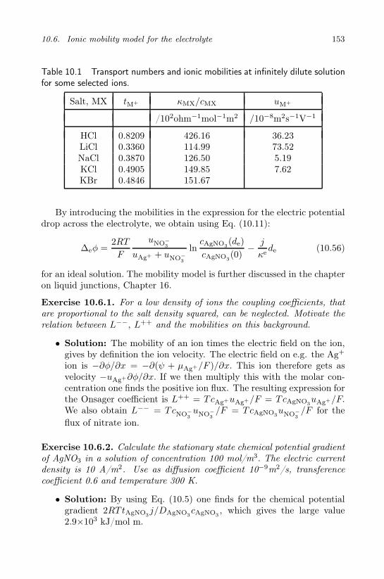
10.6. Ionic mobility model for the electrolyte 153
Table 10.1 Transport numbers and ionic mobilities at infinitely dilute solutionfor some selected ions.
Salt, MX tM+ κMX/cMX uM+
/102ohm−1mol−1m2 /10−8m2s−1V−1
HCl 0.8209 426.16 36.23LiCl 0.3360 114.99 73.52NaCl 0.3870 126.50 5.19KCl 0.4905 149.85 7.62KBr 0.4846 151.67
By introducing the mobilities in the expression for the electric potentialdrop across the electrolyte, we obtain using Eq. (10.11):
∆eφ =2RT
F
uNO−
3
uAg+ + uNO−
3
lncAgNO3
(de)
cAgNO3(0)
− j
κede (10.56)
for an ideal solution. The mobility model is further discussed in the chapteron liquid junctions, Chapter 16.
Exercise 10.6.1. For a low density of ions the coupling coefficients, thatare proportional to the salt density squared, can be neglected. Motivate therelation between L−−, L++ and the mobilities on this background.
• Solution: The mobility of an ion times the electric field on the ion,gives by definition the ion velocity. The electric field on e.g. the Ag+
ion is −∂φ/∂x = −∂(ψ + µAg+/F )/∂x. This ion therefore gets asvelocity −uAg+∂φ/∂x. If we then multiply this with the molar con-centration one finds the positive ion flux. The resulting expression forthe Onsager coefficient is L++ = TcAg+uAg+/F = TcAgNO3
uAg+/F.We also obtain L−− = TcNO−
3
uNO−
3
/F = TcAgNO3uNO−
3
/F for theflux of nitrate ion.
Exercise 10.6.2. Calculate the stationary state chemical potential gradientof AgNO3 in a solution of concentration 100 mol/m3. The electric currentdensity is 10 A/m2. Use as diffusion coefficient 10−9m2/s, transferencecoefficient 0.6 and temperature 300 K.
• Solution: By using Eq. (10.5) one finds for the chemical potentialgradient 2RTtAgNO3
j/DAgNO3cAgNO3
, which gives the large value2.9×103 kJ/mol m.

154 Chapter 10. Transport of Mass and Charge
10.7 Ionic and electronic model for the surface
Using the chemical potential for the ions in the electrolyte and for theelectrons in the conduction band in the silver, the excess entropy productionrate of the surface becomes
σs,a = Ja,ee−
(−∆a,s (µe− − Fψ)
T
)+ Je,a
Ag+
(−∆s,e
(µAg+ + Fψ
)
T
)
+ Je,a
NO−
3
−
∆s,e
(µNO−
3
− Fψ)
T
+
j
F
(−∆rG
s,a
T
)(10.57)
in the last contribution on the right hand side, we used the reaction ratethat is equal to j/F . After substituting Je,a
Ag+ = j/F+Je,aAgNO3
, Ja,ee−
= −j/Fand Je,a
NO−
3
= Je,aAgNO3
this equation becomes
σs,a = j
−(µa,e
e−− Fψa,e
)+(µe,a
Ag+ + Fψe,a)− µs,a
e−− µs,a
Ag+ + ∆rGs,a
FT
+ Je,aAgNO3
−∆s,e
(µNO−
3
+ µAg+
)
T
(10.58)
Next, we substitute φe,a = ψe,a + µe,a
Ag+/F , φa,e = ψa,e − µa,ee−/F , µAgNO3
=
µNO−
3
+ µAg+ , and ∆rGs,a = µs,a
e−+ µs,a
Ag+ + ∆nGs,a, which results in
σs,a = Je,aAgNO3
(−∆s,eµAgNO3
T
)+ j
(−∆a,eφ+ ∆nG
s,a/F
T
)(10.59)
This is Eq. (10.18), which we used. This further clarifies the relation be-tween φe,a, φa,e and ψe,a, ψa,e in the homogeneous phases and the relationbetween ∆nG
s,a and ∆rGs,a at the surface. Equation (10.59) uses the inde-
pendent fluxes and forces for the surface. It follows from Eq. (10.59) thatthe surface potential drop under reversible conditions is
∆a,eφ = −∆nGs,a
F=µs,a
Ag
F(10.60)
The corresponding Maxwell potential is
∆a,eψ = −µe,a
Ag+ + µa,ee−
− µs,aAg
F(10.61)

Part B: Applications
155

This page intentionally left blankThis page intentionally left blank

Chapter 11
Evaporation and Condensation
We study the conditions at the liquid-vapor interface during stationary evap-oration or condensation. A pure fluid is described first. The equations thatdetermine the temperature profile and the variation in the chemical po-tential, are given. The description of evaporation and condensation of amixture follows. We present resistivity coefficients for the surface obtainedusing non-equilibrium molecular dynamics and compare them with valuesfound using kinetic theory.
Evaporation or condensation occur when there is a temperature dif-ference across a liquid-vapor interface, or when the pressure in the vapordiffers from the vapor pressure of the liquid. Distillation is a process wheremixtures are separated by differences in such variables. Evaporation ofseawater by the sun is driven by a temperature difference. Significant tem-perature jumps have been measured across the surface during evaporationof water, octane, methyl-cyclohexane [160–162], aniline [163] and water-glycerol [164] around room temperatures, but also during crystallization ofHe-3 from the superfluid phase [165]. A reduction in the pressure above anoil-gas mixture, leads to evaporation of volatile components. Due to sucha pressure driven evaporation process, temperature differences of severaltens of degrees can arise in the system. This may cause damage to thepipe or block it by gas clathrate formation. Knowledge about the detailedconditions at the surface of the evaporating or condensing liquid, and thecoupling between temperature and pressure driven processes is importantfor handling technical problems in a proper way. In this chapter we shallgive governing equations for such phenomena. Bond and Struchtrup [166]have reviewed the literature on evaporation.
Consider first a liquid in equilibrium with its vapor. The thermody-namic equilibrium conditions for the surface are:
157

158 Chapter 11. Evaporation and Condensation
µgi = µl
i and T g = T l (11.1)
where µi is the chemical potential of component i, and T is the temper-ature. Superscripts g and l denote the gas (vapor) and the liquid phase,respectively. These conditions are, according to observations of Fang andWard [160–162], not fulfilled when rates of evaporation or condensation arelarge. We shall see how stationary evaporation and condensation can thenbe described by non-equilibrium thermodynamics. A detailed analysis inthis context was given earlier for a one-component system [36] and for adilute mixture [37]. Bedeaux and Kjelstrup [38] verified that the resultsof Fang and Ward could be described using this approach. We are inter-ested in expressions for the variation in the temperature and the chemicalpotentials close to and at the interface. We divide the system into threesubsystems; the liquid phase, l, the interface, s, and the gas phase, g, wherethe liquid is on the left, x < 0, and the vapor on the right, x > 0, ofthe origin. We describe a pure fluid and a two-component mixture. Val-ues for the various transport coefficients are given, using results of non-equilibrium molecular dynamics simulations [40, 67] and of kinetic theory[32–34].
We have shown elsewhere [50], using mesoscopic non-equilibrium ther-modynamics, that evaporation and condensation can be described as anactivated process. This approach is able to reproduce interesting resultsby Tsuruta and Nagayama [49] which they obtained using non-equilibriummolecular dynamics simulations. This is an interesting direction for furtherwork.
11.1 Evaporation and condensation in a pure fluid
11.1.1 The entropy production and the flux equations
Take the evaporation of a one component fluid like pure water. The evapo-ration takes place from a funnel that is partially filled, see Fig. 11.1. Fluidis supplied at a constant rate at the bottom of the funnel, while gas is with-drawn at the top at the same rate. We do not consider viscous effects, andthe pressure is constant throughout the system. The flux of fluid throughthe interface is J . The entropy production for the homogeneous phases isgiven by Eq. (4.15), which reduces for the one-component liquid to:
σl = J ′lq
∂
∂x
(1
T l
)= J ′l
q
[− 1
(T l)2
∂T l
∂x
](11.2)

11.1. Evaporation and condensation in a pure fluid 159
Figure 11.1 Sketch of experimental setup to measure temperature profilesduring evaporation. Vapor is withdrawn from the cell at the same rate asliquid is supplied. The thermocouple can be lowered to measure temperaturesnear the surface of the evaporating liquid. There is a curvature of the meniscusin the funnel container for the liquid, but the surface can be regarded as flaton a molecular scale.
The resulting flux equation is:
J ′lq = −λl
∂T l
∂x(11.3)
where λl is the thermal conductivity. These equations are also valid in thevapor phase with the sub- and superscripts l replaced by g. The thermalconductivity of the liquid is usually considerably higher than that of thevapor.
The flux of, say water, J , is constant in stationary evaporation or con-densation. The flux is the same in the liquid, across the surface and inthe gas. The measurable heat flux from the liquid into the surface, J ′l
q , ishowever, not the same as the measurable heat flux out of the surface intothe gas, J ′g
q , because heat is not conserved. The total heat flux through

160 Chapter 11. Evaporation and Condensation
the surface, Jq, is on the other hand, constant. The total heat flux is themeasurable heat flux plus the enthalpy carried by the water flux:
Jq = J ′gq +HgJ = J ′l
q +H lJ (11.4)
As frame of reference for the mass flux we have the equimolar surface ofwater [62].
The entropy production for heat and mass transport into and out of theliquid-vapor interface in a one-component system is, according to Eq. (5.15):
σs = J ′lq
[1
T s− 1
T l
]+ J ′g
q
[1
T g− 1
T s
]− J l
[µs(T s) − µl(T s)
T s
]
− Jg
[µg(T s) − µs(T s)
T s
](11.5)
For a stationary state J l = Jg = J . We can eliminate the heat flux in theliquid phase from the entropy production, using Eq. (11.4). Using Gibbs–Helmholtz’ equation
∂ (µ/T )
∂ (1/T )= H (11.6)
for the liquid as well as the vapor, we obtain to linear order in the forces
1
T s
[µg(T s) − µl(T s)
]=
1
T l
[µg(T l) − µl(T l)
]
+
∂
∂ (1/T )
[µg(T ) − µl(T )
T
]
T=T l
(1
T s− 1
T l
)
=
[µg(T l) − µl(T l)
T l
]+(Hg −H l
)( 1
T s− 1
T l
)
(11.7)
The resulting entropy production in the surface becomes the sum of twoindependent terms:
σs = J ′gq
[1
T g− 1
T l
]+ J
[−µ
g(T l) − µl(T l)
T l
]
≡ J ′gq ∆l,g
(1
T
)+ J
[−∆l,gµ(T l)
T l
](11.8)
There are thus only two independent driving forces for transport of heat andmass across the surface, a thermal force and a chemical force. The chemical

11.1. Evaporation and condensation in a pure fluid 161
potential difference across the interface is evaluated at the temperature ofthe adjacent liquid. In the stationary state, the Helmholtz energy of thesurface, which is equal to the surface tension for a one-component system,is independent of time and there is no exchange of surface energy withthe liquid or the vapor. As a consequence, the surface temperature isnot needed in the description of stationary evaporation and condensation.Alternatively, we may eliminate the heat flux in the vapor. Along the samelines we then find for the entropy production
σs = J ′lq
[1
T g− 1
T l
]+ J
[−µ
g(T g) − µl(T g)
T g
]
≡ J ′lq ∆l,g
(1
T
)+ J
[−∆l,gµ(T g)
T g
](11.9)
The standard state for the liquid is the pure liquid at p0 (1 bar) (seeAppendix 3.A). The chemical potential of the pure liquid in equilibriumwith and ideal vapor at the liquid temperature is
µl(T ) = µg,0(T ) +RT lnp∗(T )
p0(11.10)
where p∗(T ) is the pressure of the vapor in equilibrium with the liquid atthe temperature T . This pressure is referred to as the vapor pressure of theliquid or the saturation pressure. The chemical potential of an ideal vaporat the temperature T and at the real pressure, p, is:
µg(T ) = µg,0(T ) +RT lnp
p0(11.11)
By subtracting Eq. (11.10) from Eq. (11.11), we find:
−∆l,gµ(T )
T= −R ln
p
p∗(T )(11.12)
This expression assumes the gas to be ideal. For a non-ideal gas one mustreplace the pressure by the fugacity (see Appendix 3.A). The curvatureof the meniscus in Fig. 11.1 is too large to have an impact on the chem-ical potential. By substituting this relation into the entropy production,Eqs. (11.8) and (11.9), we obtain
σs = J ′gq ∆l,g(
1
T) + J
[−R ln
p
p∗(T l)
]= J ′l
q ∆l,g
(1
T
)+ J
[−R ln
p
p∗(T g)
]
(11.13)

162 Chapter 11. Evaporation and Condensation
If the temperature is continuous and the vapor pressure of the liquid islarger than the pressure in the vapor, there will be evaporation. When it islower, there is condensation. A temperature difference may also give rise toevaporation or condensation. Some temperature conditions may give riseto a vapor which is supersaturated with respect to the liquid [36].
Exercise 11.1.1. Derive that ∆l,gµ(T l) = (p − p∗(T l))/cg for any gas,using Gibbs–Duhem’s equation. Show that this is equivalent to Eq. (11.12)for an ideal gas.
• Solution: According to Gibbs–Duhem’s equation for the liquid andthe vapor, dµ = c−1dp− sdT . In global equilibrium with both phasespresent, the chemical potentials are uniquely determined by the tem-perature. Thus, for the temperature of the liquid, T l, the correspond-ing saturation pressure, p∗(T l), and chemical potential, µ∗(T l), areknown. We write
∆l,gµ(T l) = µg(T l) − µl(T l) = µg(T l) − µ∗(T l) + µ∗(T l) − µl(T l)
By using Gibbs–Duhem’s equation, it follows that
∆l,gµ(T l) = (p− p∗(T l))/cg + (p∗(T l) − p)/cl
Because cl ≫ cg it follows that ∆l,gµ(T l) = (p− p∗(T l))/cg, which iswhat we set out to derive. By using the small difference between thegas pressure and the vapor pressure of the liquid, we also have
ln[p/p∗(T l)
]= ln[1 − (p∗(T l) − p)/p∗(T l)] = −(p∗(T l) − p)/p∗(T l)
The ideal gas law then gives
R ln[p/p∗(T l)
]= (p− p∗(T l))/cgT l
which shows the equivalence.
Exercise 11.1.2. Derive the thermodynamic identity (11.6).
• Solution: We have[∂ (µ/T )
∂ (1/T )
]
p
=1
T
[∂µ
∂ (1/T )
]
p
+ µ =1
T
(∂µ
∂T
)
p
dT
d(1/T )+ µ
= −T(∂µ
∂T
)
p
+ µ

11.1. Evaporation and condensation in a pure fluid 163
where we used the chain rule in the second equality. The chemicalpotential satisfies
dµ = V dp− SdT
The derivative is, accordingly,[∂ (µ/T )
∂ (1/T )
]
p
= TS + µ = H
which proves the thermodynamic identity.
The flux equations that follow from Eq. (11.13), are either
∆l,g
(1
T
)= rs,gqq J
′gq + rs,gqµJ
−R lnp
p∗(T l)= rs,gµq J
′gq + rs,gµµJ
(11.14)
or
∆l,g
(1
T
)= rs,lqqJ
′lq + rs,lqµJ
−R lnp
p∗(T g)= rs,lµqJ
′lq + rs,lµµJ
(11.15)
Onsager relations apply, so rs,gqµ = rs,gµq and rs,lqµ = rs,lµq. Using the relationbetween the heat fluxes in the vapor and the liquid given in Eq. (11.4)and Eq. (11.6) one may derive the following relation between the interfaceresistivities for both sides of the surface:
rs,lqq = rs,gqq ≡ rsqq
rs,lqµ = rs,lµq = rs,gqµ − ∆vapHrsqq = rs,gµq − ∆vapHr
sqq
rs,lµµ = rs,gµµ − 2∆vapHrs,gµq + (∆vapH)
2rsqq
(11.16)
where we used the Onsager symmetry relations and where ∆vapH ≡Hg −H l is the enthalpy of evaporation. Because of the Onsager relationsthere are only three independent coefficients that describe the transport ofheat and mass across the surface in stationary evaporation and conden-sation. We shall use the name interface resistivities or interface transfercoefficients for the surface coefficients∗. When the heat and the mass trans-fer coefficients are negligible, the temperatures on both sides of the surfacebecome identical, while the pressure becomes equal to the vapor pressure.The liquid and the vapor close to the surface are then in equilibrium with
∗In Refs. [36–38] we absorbed a common factor T l in these interface resistivities.

164 Chapter 11. Evaporation and Condensation
one another. The temperature and pressure are then related by Clausius–Clapeyron’s equation. For larger interface resistivities, the pressure willdeviate from the vapor pressure of the liquid, and the temperatures of theliquid and the vapor close to the surface will differ from each other.
The temperature, the pressure and the mass flux can be measured.It is then convenient to write, using the Onsager relations, the flux-forcerelations in the following form
∆l,gT = − 1
λs,g
(J ′g
q − q∗,s,gJ)
−R lnp
p∗(T l)= q∗,s,g ∆l,gT
T lT g+(rs,gµµ − rs,gqq (q∗,s,g)
2)J
(11.17)
where the thermal conductivity at zero mass flux and the heat of transferat the vapor side of the surface are defined by
λs,g ≡ −[J ′g
q
∆l,gT
]
J=0
=1
T lT grs,gqqand q∗,s,g =
(J ′g
q
J
)
∆l,gT=0
= −rs,gqµ
rs,gqq
(11.18)
In the absence of a mass flux, the heat of transfer can also be found fromthe known temperatures and pressures:
q∗,s,g = −[RT lT g ln
(p/p∗(T l)
)
∆l,gT
]
J=0
(11.19)
where we used the Onsager relation.Using the measurable heat flux, one may alternatively write the flux-
force relations in the following form
∆l,gT = − 1
λs,l
(J ′l
q − q∗,s,lJ)
−R lnp
p∗(T g)= q∗,s,l ∆l,gT
T lT g+(rs,lµµ − rs,lqq
(q∗,s,l
)2)J
(11.20)
where the thermal conductivity at zero mass flux and the heat of transferat the liquid side of the surface are defined by
λs,l ≡ −[
J ′lq
∆l,gT
]
J=0
=1
T lT grs,lqq
and q∗,s,l =
(J ′l
q
J
)
∆T=0
= −rs,lqµ
rs,lqq
(11.21)

11.1. Evaporation and condensation in a pure fluid 165
In the absence of a mass flux, the heat of transfer can also be found fromthe known temperatures and pressures:
q∗,s,l = −[RT lT g ln (p/p∗(T g))
∆l,gT
]
J=0
(11.22)
where we used the Onsager relation.Bedeaux et al. [36, 37] and Kjelstrup et al. [167] used these equations
to discuss the possibility of an inverted temperature profile in front of thesurface of an evaporating fluid.
11.1.2 Interface resistivities from kinetic theory
Considerable work has been done on evaporation and condensation, usingthe kinetic theory of gases, cf. [36,37] and references therein. The resistivitytransfer coefficients of Eqs. (11.14) according to kinetic theory are [34, 36,168]:
rs,gqq =
√π
4cgeq(T s)R(T s)2vmp(T s)
(1 +
104
25π
)
rs,gqµ = rs,gµq =
√π
8T scgeq(T s)vmp(T s)
(1 +
16
5π
)
rs,gµµ =2R
√π
cgeq(T s)vmp(T s)
(σ−1 +
1
π− 23
32
)
(11.23)
Here vmp (T s) ≡√
2RT s/M is the most probable thermal velocity andM is the molar mass. The condensation coefficient, σ, is defined as thefraction of incident particles which, after collision with the liquid surface,are absorbed by the liquid. Compared to the expressions we gave in [36]we replaced all the temperatures by the temperature of the surface andtook the equilibrium coexistence density of the gas. In view of the factthat the interface resistivities are properties of the surface they should onlydepend on variables characteristic for the surface. The surface temperatureis such a variable. In molecular dynamics simulations with a relativelyshort-range Lennard-Jones spline potential [67] we found this choice to givebetter agreement with kinetic theory.
The expressions are most appropriate for hard spheres near the triplepoint. The number of moles of particles that collide with the liquid surfaceis proportional to the mean thermal velocity, vmp, times the molar densityin the gas, cg. The prefactor is characteristic for the quantity transported,
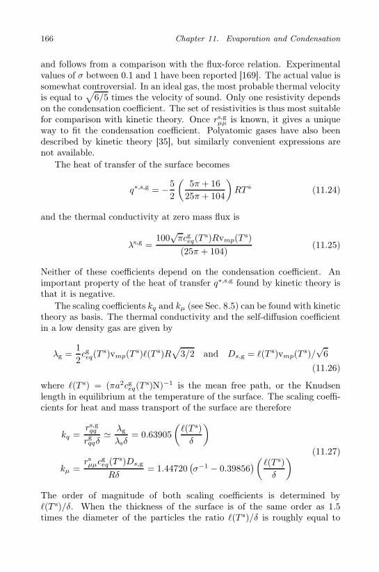
166 Chapter 11. Evaporation and Condensation
and follows from a comparison with the flux-force relation. Experimentalvalues of σ between 0.1 and 1 have been reported [169]. The actual value issomewhat controversial. In an ideal gas, the most probable thermal velocityis equal to
√6/5 times the velocity of sound. Only one resistivity depends
on the condensation coefficient. The set of resistivities is thus most suitablefor comparison with kinetic theory. Once rs,gµµ is known, it gives a uniqueway to fit the condensation coefficient. Polyatomic gases have also beendescribed by kinetic theory [35], but similarly convenient expressions arenot available.
The heat of transfer of the surface becomes
q∗,s,g = −5
2
(5π + 16
25π + 104
)RT s (11.24)
and the thermal conductivity at zero mass flux is
λs,g =100
√πcgeq(T
s)Rvmp(Ts)
(25π + 104)(11.25)
Neither of these coefficients depend on the condensation coefficient. Animportant property of the heat of transfer q∗,s,g found by kinetic theory isthat it is negative.
The scaling coefficients kq and kµ (see Sec. 8.5) can be found with kinetictheory as basis. The thermal conductivity and the self-diffusion coefficientin a low density gas are given by
λg =1
2cgeq(T
s)vmp(Ts)ℓ(T s)R
√3/2 and Ds,g = ℓ(T s)vmp(T
s)/√
6
(11.26)
where ℓ(T s) = (πa2cgeq(Ts)N)−1 is the mean free path, or the Knudsen
length in equilibrium at the temperature of the surface. The scaling coeffi-cients for heat and mass transport of the surface are therefore
kq =rs,gqq
rgqqδ≃ λg
λsδ= 0.63905
(ℓ(T s)
δ
)
kµ =rsµµc
geq(T
s)Ds,g
Rδ= 1.44720
(σ−1 − 0.39856
)( ℓ(T s)
δ
) (11.27)
The order of magnitude of both scaling coefficients is determined byℓ(T s)/δ. When the thickness of the surface is of the same order as 1.5times the diameter of the particles the ratio ℓ(T s)/δ is roughly equal to
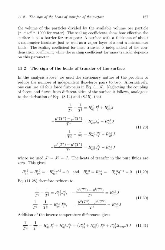
11.2. The sign of the heats of transfer of the surface 167
the volume of the particles divided by the available volume per particle(≃ cl/cg ≃ 1000 for water). The scaling coefficients show how effective thesurface is as a barrier for transport: A surface with a thickness of abouta nanometer insulates just as well as a vapor layer of about a micrometerthick. The scaling coefficient for heat transfer is independent of the con-densation coefficient, while the scaling coefficient for mass transfer dependson this parameter.
11.2 The sign of the heats of transfer of the surface
In the analysis above, we used the stationary nature of the problem toreduce the number of independent flux-force pairs to two. Alternatively,one can use all four force flux-pairs in Eq. (11.5). Neglecting the couplingof forces and fluxes from different sides of the surface it follows, analogousto the derivation of Eqs. (8.14) and (8.15), that
1
T s− 1
T l= Rs,l
qqJ′lq +Rs,l
qµJ
−µs(T s) − µl(T s)
T s= Rs,l
µqJ′lq +Rs,l
µµJ
1
T g− 1
T s= Rs,g
qq J′gq +Rs,g
qµJ
−µg(T s) − µs(T s)
T s= Rs,g
µqJ′gq +Rs,g
µµJ
(11.28)
where we used J l = Jg = J . The heats of transfer in the pure fluids arezero. This gives
Rs,lqµ = Rs,l
µq = −Rs,lqqq
∗,l = 0 and Rs,gqµ = Rs,g
µq = −Rs,gqq q
∗,g = 0 (11.29)
Eq. (11.28) therefore reduces to
1
T s− 1
T l= Rs,l
qqJ′lq , − µs(T s) − µl(T s)
T s= Rs,l
µµJ
1
T g− 1
T s= Rs,g
qq J′gq , − µg(T s) − µs(T s)
T s= Rs,g
µµJ
(11.30)
Addition of the inverse temperature differences gives
1
T g− 1
T l= Rs,l
qqJ′lq + Rs,g
qq J′gq =
(Rs,l
qq +Rs,gqq
)J ′g
q +Rs,lqq∆vapHJ (11.31)

168 Chapter 11. Evaporation and Condensation
Addition of the chemical potential differences gives
−µg(T s) − µl(T s)
T s= −µ
g(T l) − µl(T l)
T l
−[
∂
∂(1/T )
(µg
T− µl
T
)
T=T l
](1
T s− 1
T l
)
= −µg(T l) − µl(T l)
T l−Rs,l
qq∆vapHJ′lq
= −µg(T l) − µl(T l)
T l−Rs,l
qq∆vapHJ′gq −Rs,l
qq (∆vapH)2 J
=(Rs,l
µµ +Rs,gµµ
)J (11.32)
It follows that
−µg(T l) − µl(T l)
T l= Rs,l
qq∆vapHJ′gq +
(Rs,l
µµ +Rs,gµµ +Rs,l
qq (∆vapH)2)J
(11.33)
By comparing Eqs. (11.31) and (11.33) with Eq. (11.14) and Eq. (11.12),we conclude that
rs,gqq = Rs,lqq +Rs,g
qq , rs,gqµ = rs,gµq = Rs,lqq∆vapH
rs,gµµ = Rs,lµµ +Rs,g
µµ +Rs,lqq (∆vapH)
2(11.34)
Since Rs,lqq, R
s,gqq and ∆vapH are positive, q∗,s,g is negative. This is an in-
dependent confirmation of the result found in kinetic theory. Its absolutesize is given by the fraction of the thermal resistivity located on the liquidside of the surface times the latent heat, ∆vapH . It is clear that q∗,s,g hasno relation to the transported heats in the liquid and the vapor, which areboth zero. Using Eq. (11.16b) it follows that
rs,lqq = rs,gqq = Rs,lqq +Rs,g
qq , rs,lqµ = rs,lµq = −Rs,gqq ∆vapH
rs,lµµ = Rs,lµµ +Rs,g
µµ +Rs,gqq (∆vapH)
2(11.35)
This implies that q∗,s,l is positive. An important property that follows fromEqs. (11.34), (11.35) and the definition of the heat transfer coefficients is
q∗,s,g − q∗,s,l = −∆vapH (11.36)
Compare with Eq. (8.29).

11.3. Coefficients from molecular dynamics simulations 169
Using the ideal gas value of the enthalpy in the vapor, Hg = 2.5RT s,and the estimate H l = −1.5RT s for the liquid, the latent heat becomes∆vapH ≃ 4RT s. Together with the expressions (11.23) from kinetic theory,one obtains
Rs,lqq =
rs,gqµ
∆vapH=
√π
40R(T s)2cgeq(T s)vmp(T s)
(1 +
16
5π
)
Rs,gqq = rs,gqq −
rs,gqµ
∆vapH=
√π
4R(T s)2cgeq(T s)vmp(T s)
(7
8+
94
25π
)
Rs,lµµ +Rs,g
µµ = rsµµ − rsqµ∆vapH =2R
√π
cgeq(T s)vmp(T s)
(σ−1 +
1
5π− 31
32
)
(11.37)
The thermal resistivity on the vapor side is thus about 10 times the thermalresistivity on the liquid side. This depends on the choice of H l. If we reduceH l to zero this ratio decreases to 5. When we choose H l = −2.5RT s itfollows that Rs,l
µµ + Rs,gµµ is negative for σ = 1. This is why we used the
not unreasonable estimate H l = −1.5RT s. Because J l = Jg = J, it is notpossible to give expressions for Rs,l
µµ and Rs,gµµ separately.
Remark 11.1. One might think that kinetic theory gives only the resistiv-ities on the vapor side of the surface. This is not correct. Kinetic theoryuses boundary conditions, which model the whole surface. The above anal-ysis shows this very clearly.
11.3 Coefficients from molecular dynamics simulations
In non-equilibrium molecular dynamics simulations (NEMD), the computeris used to solve Newton’s equations for a many particle system. The parti-cles interact with a Lennard-Jones type potential. The way such simulationsare done is described in Chapter 22.
It was verified by Røsjorde et al. [39] and by Simon et al. [112] thatthe surface temperature was the same function of the surface tension instationary state simulations as in equilibrium simulations. This impliesthat the surface is in local equilibrium (see also Chapters 22 and 23).
NEMD was also used to determine the interface transfer coefficients ofa pure fluid [40,67,170] and of a two-component fluid [171]. The Lennard-Jones spline potential was used to describe the interparticle interaction inthese simulations. The potential minimum and the diameter were chosenidentical to those of argon in the one-component fluid.

170 Chapter 11. Evaporation and Condensation
Figure 11.2 The main coefficients for heat transfer, rsqq = rs,gqq = rs,lqq, from
NEMD simulations in m2s J−1K−1, as a function of the surface tension. Thedashed line is the value predicted by kinetic theory. Reproduced from J. ColloidInterface Sci. 299 (2006) 452–463 with permission from Elsevier.
Figures 11.2–11.4 show the results of the simulations for the interfaceresistivities in the pure fluid [67]. The resistivities are plotted as functionsof the surface tension. The surface tension increases as we move from thecritical point (γ = 0) to the triple point in the phase diagram.
In Figs. 11.2 and 11.4 the values predicted by kinetic theory are plottedas dashed, dotted or dash-dotted lines. All interface resistivities go to zerotowards the critical point, when γ = 0. As the liquid and the vapor be-come indistinguishable in that limit, this is to be expected. The variationobserved in the figures as a function of the surface tension is therefore phys-ically reasonable. The surface tension is a unique function of the surfacetemperature. A high surface tension corresponds to a low temperature. Atthe triple point, the vapor is closest to being ideal. The surface has itsmaximum resistance to transfer of both heat and mass close to the triplepoint.
Figure 11.4 shows that the coupling coefficients, rs,gqµ , rs,gµq on the vaporside and rs,lqµ, rs,lµq on the liquid side, satisfy the Onsager symmetry relationswithin the accuracy of the simulation. These simulations [67] were thefirst simulations which verified the validity of the Onsager relations for thesurface. In Fig. 11.5, the resulting heats of transfer are plotted. These arelabelled q∗,s,gqµ , q∗,s,gµq and q∗,s,lqµ , q∗,s,lµq to indicate the cross coefficient from
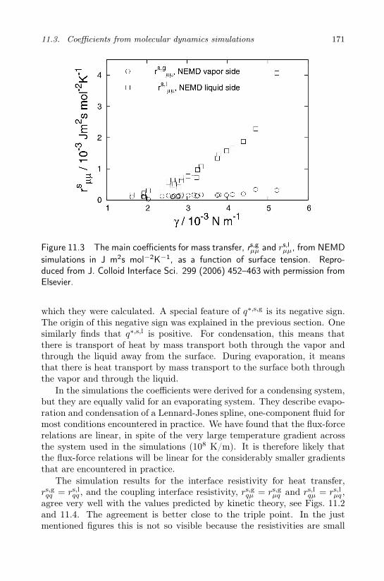
11.3. Coefficients from molecular dynamics simulations 171
Figure 11.3 The main coefficients for mass transfer, rs,gµµ and rs,lµµ, from NEMD
simulations in J m2s mol−2K−1, as a function of surface tension. Repro-duced from J. Colloid Interface Sci. 299 (2006) 452–463 with permission fromElsevier.
which they were calculated. A special feature of q∗,s,g is its negative sign.The origin of this negative sign was explained in the previous section. Onesimilarly finds that q∗,s,l is positive. For condensation, this means thatthere is transport of heat by mass transport both through the vapor andthrough the liquid away from the surface. During evaporation, it meansthat there is heat transport by mass transport to the surface both throughthe vapor and through the liquid.
In the simulations the coefficients were derived for a condensing system,but they are equally valid for an evaporating system. They describe evapo-ration and condensation of a Lennard-Jones spline, one-component fluid formost conditions encountered in practice. We have found that the flux-forcerelations are linear, in spite of the very large temperature gradient acrossthe system used in the simulations (108 K/m). It is therefore likely thatthe flux-force relations will be linear for the considerably smaller gradientsthat are encountered in practice.
The simulation results for the interface resistivity for heat transfer,rs,gqq = rs,lqq , and the coupling interface resistivity, rs,gqµ = rs,gµq and rs,lqµ = rs,lµq ,agree very well with the values predicted by kinetic theory, see Figs. 11.2and 11.4. The agreement is better close to the triple point. In the justmentioned figures this is not so visible because the resistivities are small

172 Chapter 11. Evaporation and Condensation
-14
-12
-10
-8
-6
-4
-2
0
2
1 2 3 4 5 6 7rsm
qand r
sq
m/ 10
-7m
2s m
ol-1
K-1
g / 10-3
N m-1
rs,g
mq, vapor side
rs,g
q m, vapor side
rs,l
mq, liquid side
rs,l
q m, liquid side
Figure 11.4 The coupling coefficients for heat and mass transfer, rs,gqµ, rs,gµq
and rs,lqµ, rs,lµq from NEMD simulations (in m2s mol−1K−1), as a function of thesurface tension. The dotted and the dash-dotted lines are the predictions fromkinetic theory. Reproduced from J. Colloid Interface Sci. 299 (2006) 452–463with permission from Elsevier.
close to the critical point. In Fig. 11.5 for the heats of transfer, which arethe ratios of two interface resistivities, this lack of agreement close to thecritical point is more clearly visible. This agreement of the simulation datawith kinetic theory is special for the Lennard-Jones spline potential. Thereis no such agreement for the simulations for octane [112] or for a cut-offLennard-Jones potential [167]. In recent simulations using a longer rangeLennard-Jones spline potential, we found that in particular the size of thecoupling coefficient increases substantially above the kinetic theory value.
The value predicted by kinetic theory for the interface resistivity to masstransfer on the vapor side, rs,gµµ, contains the condensation coefficient. Itwas possible to fit this coefficient using the values obtained for the interfaceresistivity in the NEMD simulations using a Lennard-Jones spline potential,see Fig. 11.6. The accuracy of the resulting values is about 20%. The valueincreases from a value near 0.1 near the critical point to a value of about 0.8near the triple point. The value is reasonable, and agrees with moleculardynamics simulations by Tsuruta and Nagayama [172].
Kinetic theory and NEMD are helpful in the sense that they give amechanistic picture of the collision of particles in the vapor phase with

11.3. Coefficients from molecular dynamics simulations 173
Figure 11.5 The heats of transfer, q∗,s,gqµ , q∗,s,gµq and q∗,s,lqµ , q∗,s,lµq from NEMD
simulations (in kJ mol−1), as a function of the surface tension. Reproducedfrom J. Colloid Interface Sci. 299 (2006) 452–463 with permission fromElsevier.
Figure 11.6 The condensation coefficient for molecular dynamics simulationsof a fluid using a Lennard-Jones spline potential as a function of the surfacetension. Reproduced from J. Colloid Interface Sci. 299 (2006) 452–463 withpermission from Elsevier.

174 Chapter 11. Evaporation and Condensation
the liquid surface. The NEMD simulations for the relatively short-rangeLennard-Jones spline fluid reproduced the interface resistivities from kinetictheory along the coexistence curve from the triple point until about halfwayto the critical point. The density of the vapor is lowest close to the triplepoint. It is therefore not unexpected that the agreement between simulatedand computed results is best near the triple point. As the Lennard-Jonesspline vapor is still far from ideal in the triple point, the agreement is betterthan what one might have expected.
The values of the interface resistivities found from both NEMD simula-tions and from kinetic theory lead to discontinuities in the temperature atthe surface of a few tenths of a degree rather than a few degrees. As shownby Bedeaux and Kjelstrup [38] it is necessary to use much larger interfaceresistivities to explain the temperature differences of several degrees foundby Fang and Ward [160–162] or Phillips and coworkers [163,164,173]. Thenon-equilibrium van der Waals square gradient model contains a free pa-rameter related to the behavior of the thermal resistivity in the interfacialregion. This makes it possible to model larger interfacial resistivities [108].It is interesting to study their relative size, but it does not resolve thequestion of why they are possibly so large.
Exercise 11.3.1. Consider stationary evaporation of water. The liquidenters the evaporation chamber at x = −2 cm with room temperature (300K), and is evacuated by an under-pressure of 2 Pa at x = 2 cm with roomtemperature. The liquid-vapor interface is at x = 0. The temperature atthe liquid side of the surface is 0.9 oC. At the vapor side of the surface, thetemperature is −2.8 oC.
Calculate the temperature profile, the heat fluxes and the mass flux, usinga saturation pressure of 600 Pa and a heat of evaporation of 45 kJ/mol[174]. Find the transfer coefficients for transport across the surface. Users,gµq = rs,gqµ = 0.01∆vapH rs,gqq for the coupling coefficients. The thermalconductivity of liquid water and water-vapor are 0.61 and 0.018 J/Kms[114], respectively.
• Solution: In the liquid as well as in the vapor we have
∂Jq/∂x = ∂J ′q/∂x+ ∂(hJ)/∂x = −∂ (λ∂T/∂x)∂x+ ∂(hJ)/∂x = 0
cf. Eqs. (11.3) and (11.4). As λ, h and J are all constant it followsthat ∂T/∂x is constant, so that T is a linear function of position.Therefore, we have
T l(x) = T l(0) + (x/0.02)(T l(0) − 300) = T l,g + (x/0.02)(T l,g − 300)
T g(x) = T g(0) − (x/0.02)(T g(0) − 300) = T g,l − (x/0.02)(T g,l − 300)

11.3. Coefficients from molecular dynamics simulations 175
The resulting heat fluxes in the liquid and the vapor are constant,cf. Eq. (11.3), and given by:
J ′lq = −30.5(T l,g − 300) = 793 and J ′g
q = 0.9(T g,l − 300) = −26.7
in J/m2s. Heat needed to provide the enthalpy of evaporation isconducted to the surface from the gas as well as from the liquid.
The constant mass flux is obtained from the energy balance
J =J ′l
q − J ′gq
∆vapH= 0.017 mol/m2s
The driving forces are
∆l,gT
T l,gT g,l= −274.05− 270.35
270.35× 274.05= −0.5 × 10⁻⁴ /K
Rlnp
p∗= 8.314 × ln
(598
600
)= −2.8 × 10⁻² J/mol K
With knowledge of the fluxes and forces, there are three unknowncoefficients in the flux equations for the surface. Substituting also therelation given for the coupling resistivities, we find
∆l,gT
T l,gT g,l= −26.7rs,gqq + 0.017rs,gqµ = − (26.7 − 0.00017∆vapH) rs,gqq
= −19.0rs,gqq = −0.5 × 10⁻⁴ /K
−Rlnp
p∗= −26.7rs,gµq + 0.017rs,gµµ = −0.267∆vapHr
s,gqq + 0.017rs,gµµ
= −12000rs,gqq + 0.017rs,gµµ = 2.8 × 10⁻²J/mol K
By solving the two unknowns from these equations, and obtaining thecoupling resistivity using the expression given above, we find
rs,gqq = 2.63 × 10⁻⁵ m2s/JK, rs,gµq = rs,gqµ = 1.18 × 10⁻² m2s/mol K
rs,gµµ = 20.2 J m2s/mol2K
These values are about 3 orders of magnitude larger than the valuesone would obtain from kinetic theory. The temperature and pres-sure differences predicted by kinetic theory for this case are too smallto measure.

176 Chapter 11. Evaporation and Condensation
The exercise above used tabulated thermodynamic and transport data forwater, but the temperature jump and pressure difference were chosen asan example. The calculated transfer coefficients are therefore not realistic.Water has a very large heat of evaporation. In such a case, one mustuse a heat of transfer that is substantially smaller than the enthalpy ofevaporation in order to obtain a measurable temperature difference. Theratio of q∗,s,g and ∆vapH of 0.18 predicted by the kinetic theory for themonatomic fluid, is then much too large. In the exercise, the value 0.01was used. Larger values would lead to negative values of rs,gµµ for the giventemperature difference, which is not allowed.
11.4 Evaporation and condensation in a two-component fluid
11.4.1 The entropy production and the flux equations
Consider again the liquid funnel in Fig. 11.1, but now with a solute in thesolvent. The solvent can be for instance, water. The solute can be anelectrolyte, like NaCl, an organic compound with a low vapor pressure, likeglycerol, or an organic compound with high vapor pressure, like ethanol.The liquid is on the left, x < 0, and the vapor on the right, x > 0. Theentropy production for the liquid phase is given by Eq. (4.15):
σl = J ′lq
∂
∂x
(1
T l
)+ Jsol
[− 1
T l
∂µlsol,T
∂x
](11.38)
The subscript “sol” indicates solute, and J lsol is the (molar) flux of the solute.
The flux equations are
∂
∂x
(1
T l
)= rlqqJ
′lq + rlqsJ
lsol
− 1
T l
∂µlsol,T
∂x= rlsqJ
′lq + rlssJ
lsol
(11.39)
The chemical potential of a non-electrolyte solute is:
µlsol = µ0,l
sol +RT ln(clsolylsol) (11.40)
where clsol is the molar concentration of the solute, ylsol the activity co-
efficient (equal to unity for Henrian solutions), and µ0,lsol is the chemical
potential in the standard state (of 1 molal), see Appendix 3.A. We assumeideal solution, yl
sol = 1, and neglect the Soret effect, rlqs = rlsq = 0. This
11.4. Evaporation and condensation in a two-component fluid 177
reduces the above equations to:
J ′lq = − 1
(T l)2rlqq
∂T l
∂x= −λl
sol
∂T l
∂x
J lsol = − 1
T lrlss
∂µlsol,T
∂x= − R
clsolrlss
∂clsol∂x
= −Dlsol
∂clsol∂x
(11.41)
The last equation is new compared to Sec. 11.2. It gives the flux of thesolute in the liquid phase. In the vapor phase all the above equations arethe same with the super- or subscript l replaced by g.
In the description of the surface we use the equimolar surface of thesolvent as the frame of reference for the fluxes. The solvent flux, Jw, isthen constant through the surface, but the solute flux is not necessarilyconstant through the surface. Usually, there is adsorption of solute at thesurface:
dΓsol
dt= J l
sol − Jgsol (11.42)
Adsorption of solute at the surface reduces the surface tension. In a station-ary system, the concentration of solute and its absorption at the surfaceare constant everywhere, so that not only Jw, but also Jsol is constantthroughout the system. The analysis in this chapter is restricted to thiscase.
The measurable heat flux from the liquid into the surface, J ′lq , is not
the same as the measurable heat flux out of the surface into the gas, J ′gq ,
because the enthalpies differ in the two phases. The total heat flux in thesystem, Jq, is the conserved flux. The total heat flux is the measurableheat flux plus the enthalpy carried by the solvent and the solute fluxes. Ina stationary state Jq is constant throughout the system and one has:
Jq = J ′gq +Hg
wJw +HgsolJsol = J ′l
q +H lwJw +H l
solJsol (11.43)
The entropy production for the liquid-vapor interface in the two-component system is analogous to Eq. (8.13):
σs = J ′lq ∆l,s
(1
T
)+ J ′g
q ∆s,g
(1
T
)+ Jsol
[− 1
T s∆l,gµsol,T (T s)
]
+ Jw
[− 1
T s∆l,gµw,T (T s)
](11.44)
The chemical potential differences are evaluated at temperature T s, cf.Eq. (5.19). The heat flux in the liquid may be eliminated using Eq. (11.43).

178 Chapter 11. Evaporation and Condensation
Following the procedure outlined in Sec. 11.1.1, this results in
σs = J ′gq ∆l,g
(1
T
)+ Jsol
[− 1
T l∆l,gµsol,T (T l)
]+ Jw
[− 1
T l∆l,gµw,T (T l)
]
(11.45)where the chemical potential differences are now evaluated at the temper-ature of the liquid, T l. For the solvent and the solute we will again useEqs. (11.10)–(11.13) to express the chemical potential differences in thepartial pressures. The force conjugate to Jw is therefore:
− 1
T l∆l,gµw,T (T l) = −R ln
pgw
pg∗w (T l)
(11.46)
and the force conjugate to Jsol is:
− 1
T l∆l,gµsol,T (T l) = −R ln
pgsol
pg∗sol(T
l)(11.47)
The partial pressures are divided by the partial pressures for saturatedvapor at the temperature of the liquid, T l. When the vapor is not ideal,we must use the fugacities instead of the pressures, see Appendix 3.A.Expressions for activity coefficients in non-ideal gas and in liquid mixturescan be found in Perry [114].
The flux equations derived from Eq. (11.45), together with Eqs. (11.46)and (11.47), are:
J ′gq = ls,gqq ∆l,g
(1
T
)+ ls,gqs
(−R ln
pgsol
pg∗sol(T
l)
)+ ls,gqw
(−R ln
pgw
pg∗w (T l)
)
Jsol = ls,gsq ∆l,g
(1
T
)+ ls,gss
(−R ln
pgsol
pg∗sol(T
l)
)+ ls,gsw
(−R ln
pgw
pg∗w (T l)
)
Jw = ls,gwq∆l,g
(1
T
)+ ls,gws
(−R ln
pgsol
pg∗sol(T
l)
)+ ls,gww
(−R ln
pgw
pg∗w (T l)
)
(11.48)
The reason to use conductivities in this case is that this simplifies thedefinition of the heats of transfer and of the co-transfer coefficient. In thefollowing subsection, we will also give the linear laws using resistivities. Inaddition to the heat of transfer for the solvent, we define the heat of transferfor the solute:
q∗s,gw ≡(J ′g
q
Jw
)
∆T=∆µsol=0
=ls,gqw
ls.gww
q∗s,gsol ≡(J ′g
q
Jsol
)
∆T=∆µw=0
=ls,gqs
ls.gss
(11.49)

11.4. Evaporation and condensation in a two-component fluid 179
We also define the co-transfer coefficient :
τ s,gsol ≡
(Jsol
Jw
)
∆T=∆µsol=0
=ls,gsw
ls,gww(11.50)
By introducing the heats of transfer and the co-transfer coefficient, thelinear relations become:
J ′gq = ls,gqq ∆l,g
(1
T
)− q∗s,gsol l
s,gss R ln
pgsol
pg∗sol
− q∗s,gw ls,gwwR lnpgw
pg∗w
Jsol = q∗s,gsol ls,gss ∆l,g
(1
T
)− ls,gss R ln
pgsol
pg∗sol
− τ s,gsol l
s,gwwR ln
pgw
pg∗w
Jw = q∗s,gw ls,gww∆l,g
(1
T
)− τ s,g
sol ls,gwwR ln
pgsol
pg∗sol
− ls,gwwR lnpgw
pg∗w
(11.51)
These equations govern evaporation and condensation of a binary idealmixture.
11.4.2 Interface resistivities from kinetic theory
Kinetic theory gives equations of transport also for more components [34].Take the case of a solvent with one solute. Kinetic theory uses two con-densation coefficients, σsol and σw, for the solute and the solvent particlesrespectively. The condensation coefficients give the fractions of particlesabsorbed by the liquid surface. The rest is reflected with a Boltzmanndistribution of velocities at the temperature of the liquid [37].
The resistivity coefficients are the inverse of the conductivity coeffi-cients, given byls,gqq ls,gqs,g ls,gqw
ls,gs,gq ls,gss ls,gsw
ls,gwq ls,gws ls,gww
×
rs,gqq rs,gqs rs,gqw
rs,gsq rs,gss rs,gsw
rs,gwq rs,gws rs,gww
=
1 0 0
0 1 0
0 0 1
(11.52)
With these resistivities, the linear relations become
∆l,g
(1
T
)= rs,gqq J
′gq + rs,gqs Jsol + rs,gqwJw
−R lnpgsol
pg∗sol(T
l)= rs,gsq J
′gq + rs,gss Jsol + rs,gswJw
−R lnpgw
pg∗w (T l)
= rs,gwqJ′gq + rs,gwsJsol + rs,gwwJw
(11.53)

180 Chapter 11. Evaporation and Condensation
Kinetic theory now gives [37, 168]†:
rs,gqq =
√π
4R(T s)2cgeq(T s)vmp(T s)
×
1 +104
25π
(λg
sol
λg
)2[1 +
cgwcgsol
4
√Msol
Mw
]
+
(λg
w
λg
)2[1 +
cgsolcgw
4
√Mw
Msol
]
rs,gss =R√π
16cgeq(T s)vmp(T s)
1 + 32
[σ−1
sol +1
π− 3
4
] [1 +
cgwcgsol
4
√Msol
Mw
]
rs,gww =R√π
16cgeq(T s)vmp(T s)
1 + 32
[σ−1
w +1
π− 3
4
] [1 +
cgsolcgw
4
√Mw
Msol
]
rs,gqs = rs,gsq =
√π
8T scgeq(T s)vmp(T s)
1 +
16λgsol
5πλg
[1 +
cgwcgsol
4
√Msol
Mw
]
rs,gqw = rs,gwq =
√π
8T scgeq(T s)vmp(T s)
1 +
16λgw
5πλg
[1 +
cgsolcgw
4
√Mw
Msol
]
rs,gsw = rs,gws =R√π
16cgeq(T s)vmp(T s)
(11.54)
In these expressions vmp(Ts) is the average of the most probable velocities
of the two components at temperature T s:
vmp = (cgsolvsol,mp + cgwvw,mp)/cg (11.55)
with
vsol,mp =√
2RT s/Msol and vw,mp =√
2RT s/Mw (11.56)
Expressions Eq. (11.23) for the one-component system gave the interfaceresistivities as function of variables characteristic for the surface. In theequations (11.54) we therefore again used the surface temperature and the
†The formulae given in [37] contained errors which are corrected in the expressionsgiven below, see [175].

11.4. Evaporation and condensation in a two-component fluid 181
densities at equilibrium at this temperature, rather than the temperatureand densities of the gas as used before [37, 175].
The thermal conductivity is the sum of the contributions due to bothcomponents,
λg = λgsol + λg
w (11.57)
where
λgsol =
1
3ℓsolvsol,mpc
gsolC
gsol,V and λg
w =1
3ℓwvw,mpc
gwC
gw,V (11.58)
Here ℓi and Cgi,V are the mean free path and the partial specific heat at
constant volume of component i. The molar density in the gas is
cg = cgsol + cgw (11.59)
Even though this is not explicitly indicated everywhere, the equilibriumvalue is used for all quantities in Eqs. (11.54)–(11.59) at the temperature ofthe surface, T s. This is an improvement compared to the expressions givenin [37, 175].
A special case of interest is the dilute solution, when only a small amountof solute is present. In that case
cgsol ≪ cgw ≃ cg, λgsol ≪ λg
w ≃ λg, cgsol,V ≪ cgw,V ≃ cgV (11.60)
The resistivity coefficients then simplify to
rs,gqq =
√π
4R(T s)2cgeq(T s)vmp(T s)
(1 +
104
25π
)
rs,gss =2R
√π
cgsolvmp(T s)
(σ−1
sol +1
π− 3
4
)4
√Msol
Mw
rs,gww =2R
√π
cgeq(T s)vmp(T s)
(σ−1
w +1
π− 23
32
)
rs,gqs = rs,gsq =
√π
8T scgeq(T s)vmp(T s)
(1 +
16λgsolc
geq
5πλgcgsol
4
√Msol
Mw
)
rs,gqw = rs,gwq =
√π
8T scgeq(T s)vmp(T s)
(1 +
16
5π
)
rs,gsw = rs,gws =R√π
16cgeq(T s)vmp(T s)
(11.61)
Even though this is not explicitly indicated everywhere, the equilibriumvalue is used for all quantities in Eqs. (11.60) and (11.61) at the temperature

182 Chapter 11. Evaporation and Condensation
of the surface, T s. The resistivities rs,gqq , rs,gqw = rs,gwq and rs,gww are identical tothose given in Sec. 11.1.2 for the one-component case. A small concentrationof solute does thus not change these coefficients. In the linear relations forthe forces and fluxes, Eq. (11.53), one may use the fact that Jg
sol is small,like cgsol. This implies, given the value of the coupling coefficients, that
∆l,g
(1
T
)= rs,gqq J
′gq + rs,gqwJw
−R lnpgw
pg∗w (T l)
= rs,gwqJ′gq + rs,gwwJw
(11.62)
The heat and solvent fluxes are consequently not affected by the solute ifit is sufficiently dilute. The analysis in Sec. 11.1 is adequate for that case.For the solute one has
−R lnpgsol
pg∗sol(T
l)= rs,gsq J
′gq + rs,gss Jsol + rs,gswJw (11.63)
In this expression, it is important that rs,gss is inversely proportional to cgsolso that the term rs,gss J
gsol is of the same order of magnitude as the other two
terms. Therefore, if the overall concentration of solute is small, one mayhave a backup of solute in front of the surface. This may lead locally toconsiderable concentration gradients, in which case the coupling to Jg
sol willbecome important. It was shown that the solute concentration is negligible,as long as the equilibrium temperature and concentrations in the vaporsatisfy
cgsolcgeq(T s)
≪ ∆Hw,vap
RT
ℓ
dg(11.64)
where dg is the thickness of the vapor phase [37]. This is a rather smallupper bound on the concentration of the solute in most cases. It is oftendifficult in practice to purify fluids sufficiently to avoid solute trace elements[176]. Non-equilibrium molecular dynamics simulations avoid this difficulty[171].

Chapter 12
Multi-Component Heat and
Mass Diffusion
In this chapter we describe multi-component mass and heat transport ina heterogeneous system. After a general introduction about the homoge-neous phases, we discuss the Maxwell–Stefan equations for multi-componentdiffusion in the presence of a temperature gradient. We then discuss thetransport of mass and heat through the surface and combine the descrip-tion of the two homogeneous phases with the one for the surface. We alsodiscuss multi-component diffusion in the homogeneous phase using variousframes of reference.
Diffusion takes place in all chemical mixtures and is often the ratelimiting process. The simplest equation that describes diffusion of onecomponent in another is Fick’s law, Eq. (1.2). The diffusion of one com-ponent is often influenced by concentration gradients of other components,however. In other words, there is coupling of diffusion fluxes. Such cou-pling is efficiently described using the Maxwell–Stefan equations [42, 69].Also heat is transported along with components, so diffusion couples toheat transport.
In the following section, we explain how we can obtain Maxwell–Stefan equations including coupling of heat and mass transport, withinthe context of non-equilibrium thermodynamics. We also show howthese equations are related to other descriptions of multi-componentdiffusion, and how they can be combined to deal with interfacetransport.
183
184 Chapter 12. Multi-Component Heat and Mass Diffusion
12.1 The homogeneous phases
Consider an isobaric, nonisothermal system with three components in ahomogeneous phase∗. There are then three independent driving forces inthe system, one thermal and two component driving forces. In order to dealwith the components on the same footing, however, we write the entropyproduction using four forces:
σ = Jq∂
∂x
1
T− JA
∂
∂x
µA
T− JB
∂
∂x
µB
T− JC
∂
∂x
µC
T
= J ′q
∂
∂x
1
T− vA
cAT
∂µA,T
∂x− vB
cBT
∂µB,T
∂x− vC
cCT
∂µC,T
∂x(12.1)
where the velocity of component i (i = A, B or C) is defined by vi ≡ Ji/ci.We have suppressed the superscript i or o, indicating the phase, as theexpressions are the same in both phases. For stationary states, the totalheat flux, Jq = J ′
q + HAJA + HBJB + HCJC, and the molar fluxes, Jj ,are constant throughout the system. The component forces are related byGibbs–Duhem’s equation
cA∂µA,T
∂x+ cB
∂µB,T
∂x+ cC
∂µC,T
∂x= 0 (12.2)
Only two of these forces are therefore independent.Following Eq. (12.1), the equations for the thermodynamic forces can
be written as
∂
∂x
1
T= rqqJ
′q + rqAvA + rqBvB + rqCvC
−cAT
∂µA,T
∂x= rAqJ
′q + rAAvA + rABvB + rACvC
−cBT
∂µB,T
∂x= rBqJ
′q + rBAvA + rBBvB + rBCvC
−cCT
∂µC,T
∂x= rCqJ
′q + rCAvA + rCBvB + rCCvC
(12.3)
The sum of three terms on the left hand side of Eq. (12.3) is zero accord-ing to Gibbs–Duhem’s equation. Onsager relations were shown to applyin Eq. (12.3), when the forces depend via Gibbs–Duhem’s equation, see
∗For a discussion of the nonisobaric system with an arbitrary number of components,see Kuiken [31], and Krishna and coworkers [42, 69].

12.1. The homogeneous phases 185
de Groot and Mazur [20], page 67. This gives:
rAq = rqA, rBq = rqB, rCq = rqC
rAB = rBA, rAC = rCA, rBC = rCB
(12.4)
As Eqs. (12.3) hold for any arbitrary measurable heat flux and arbitraryvelocities of the components, it follows that the resistivities in the matrixare dependent, and satisfy
rAq + rBq + rCq = 0
rAA + rBA + rCA = 0
rAB + rBB + rCB = 0
rAC + rBC + rCC = 0
(12.5)
From the Onsager relations, it follows that also
rqA + rqB + rqC = 0
rAA + rAB + rAC = 0
rBA + rBB + rBC = 0
rCA + rCB + rCC = 0
(12.6)
There are thus only six independent resistivities. Once these have beenobtained from experiments, the others can be calculated using the aboverelations. The resistivity matrix has an eigenvalue equal to zero, and thusa zero determinant. It cannot therefore be inverted into a conductivitymatrix!
For our further analysis, it is convenient to write Eq. (12.3) in the fol-lowing form
∂T
∂x= − 1
λ
(J ′
q − cAq∗AvA − cBq
∗BvB − cCq
∗CvC
)
cAT
∂µA,T
∂x= −cAq
∗A
T 2
∂T
∂x−RAAvA −RABvB −RACvC
cBT
∂µB,T
∂x= −cBq
∗B
T 2
∂T
∂x−RBAvA −RBBvB −RBCvC
cCT
∂µC,T
∂x= −cCq
∗C
T 2
∂T
∂x−RCAvA −RCBvB −RCCvC
(12.7)

186 Chapter 12. Multi-Component Heat and Mass Diffusion
where the thermal conductivity, the measurable heats of transfer and theresistivities for component fluxes at constant temperature are defined by:
λ ≡ 1
T 2rqq, cjq
∗j ≡ − rqj
rqq
and Rjk ≡ rjk − rjqrqk
rqqfor j, k = A, B or C (12.8)
The measurable heats of transfer satisfy, see Eq. (12.5a),
cAq∗A + cBq
∗B + cCq
∗C = 0 (12.9)
The resistivities for mass flow at constant temperature satisfy, seeEq. (12.5),
RAA +RBA +RCA = 0
RAB +RBB +RCB = 0
RAC +RBC +RCC = 0
(12.10)
From the Onsager relations, cf. Eq. (12.6), it follows that also
RAA +RAB + RAC = 0
RBA +RBB +RBC = 0
RCA +RCB +RCC = 0
(12.11)
Using Eqs. (12.9) and (12.11) in Eq. (12.7), one may verify that the right(and therefore the left) hand sides are independent of the choice of theframe of reference. Possible choices of the velocity vref of the frame ofreference, see Section 4.4 [20], are the center of mass, the average volume,the average molar velocity and the solvent velocity. We discuss these choicesin Sec. 12.4.
12.2 The Maxwell–Stefan equations for multi-component
diffusion
The Maxwell–Stefan equations give a convenient way to describe multi-component diffusion [31, 42] because the description is independent of theframe of reference, and the diffusion coefficients contain binary interdif-fusion coefficients. Such coefficients are easily available from experiments[139].

12.2. The Maxwell–Stefan equations for multi-component diffusion 187
The Maxwell–Stefan diffusion coefficients, Ðjk, are defined from†
RAB ≡ −cRxAxB
ÐAB, RAC ≡ −cRxAxC
ÐAC, RBC ≡ −cRxBxC
ÐBC(12.12)
where xi ≡ ci/c is the mole fraction of component i, and the diagonalcoefficients, RAA, RBB and RCC, are found from Eq. (12.11). The Maxwell–Stefan diffusion coefficients are symmetric, Ðjk=Ðkj. The heats of transfercan be written in terms of the thermal diffusion coefficients, DT,j , such thatthey satisfy Eq. (12.9), as
q∗j ≡n∑
k 6=j
RTxk
Ðjk
(DT,j
ρj− DT,k
ρk
)(12.13)
Here ρj ≡ cjMj is the mass density in kg/m3 and Mj the molar weight inkg/mol of component j. Using Eqs. (12.9) and (12.12) we can write thelinear laws (12.7) in the following form
∂T
∂x= − 1
λ
[J ′
q − cBq∗B (vB − vA) − cCq
∗C (vC − vA)
]
xB
RT
∂µB,T
∂x= −xBq
∗B
RT 2
∂T
∂x+xAxB
ÐAB(vA − vB) +
xBxC
ÐBC(vC − vB)
xC
RT
∂µC,T
∂x= −xCq
∗C
RT 2
∂T
∂x+xAxC
ÐAC(vA − vC) +
xBxC
ÐBC(vB − vC)
(12.14)
We left the equation for ∂µA,T /∂x out as it is redundant. It follows fromthe last two equations using Gibbs–Duhem’s equation. To keep the ex-pression a bit more elegant we did not substitute the expressions for themeasurable heats of transfer in terms of the thermal diffusion coefficients.Only velocity differences enter. The description is thus independent of theframe of reference.
Binary diffusion coefficients are reasonably well known [31,69,139,177].Heats of transfer are not so well known. Approximate expressions havebeen given by Kempers [145,178] and by Haase [22] for binary mixtures, seeSec. 8.2. Given the Maxwell–Stefan diffusion coefficients, one can calculatethe resistivities RAB, RAC and RBC, using Eq. (12.12) and then the diagonalcoefficients, RAA, RBB and RCC, using Eq. (12.11). Using also the thermalconductivity and the heats of transfer, the resistivities rqq, rqk = rjq andrjk = rkj follow from Eq. (12.8).
†We follow Krishna and Wesselingh [42] in this definition rather than Kuiken [31] whouses the pressure p instead of cRT .
188 Chapter 12. Multi-Component Heat and Mass Diffusion
The chemical potentials of the components;
µi = µ0i (T ) +RT lnxiγi (12.15)
where µ0i (T ) is the standard chemical potential, xi is the mole fraction and
γi is the activity coefficient, give relations between the chemical potentialat constant temperature and the gradient in mole fraction:
xi
RT
∂µi,T
∂x=∂xi
∂x
(1 +
∂ ln γi
∂ lnxi
)(12.16)
Remark 12.1. The use of the Maxwell–Stefan formalism for diffusion hasa number of important advantages: In the first place, the diffusion coef-ficients are symmetric for the interchange of components, this is contraryto all other descriptions of multi-component diffusion. In the second place,the formalism is valid in an arbitrary frame of reference, also contrary toother descriptions. A third property, found experimentally and which isvery useful, is that the Maxwell–Stefan diffusion coefficients are rather in-dependent of the concentrations [31, 42]. Finally, it is also found that thecoefficient for two given components remains more or less the same if thethird component is changed. This makes it possible to model diffusion inmulti-component mixtures with data from binary mixtures.
12.3 The Maxwell–Stefan equations for the surface
Maxwell–Stefan equations for the surface have their basis in the entropyproduction of the surface. Equation (5.15) is used to give a formulation interms of velocities:
σs = J ′iq ∆i,s
(1
T
)+ J ′o
q ∆s,o
(1
T
)+
∑
j=A,B,C
J ij
(−∆i,sµj,T
T s
)
+∑
j=A,B,C
Joj
(−∆s,oµj,T
T s
)
= J ′iq ∆i,s
(1
T
)+ J ′o
q ∆s,o
(1
T
)+
∑
j=A,B,C
vij
(−cijT s
∆i,sµj,T
)
+∑
j=A,B,C
voj
(−cojT s
∆s,oµj,T
)(12.17)
All velocities in the equations for the excess entropy production have thesurface as their frame of reference. Assuming that there are no coupling

12.3. The Maxwell–Stefan equations for the surface 189
coefficients from one side of the surface to the other, the equations for thethermodynamic forces can be written as
∆i,s
(1
T
)= rs,iqqJ
′iq + rs,iqAvi
A + rs,iqBviB + rs,iqCvi
C
− ciA
T s∆i,sµA,T = rs,iAqJ
′iq + rs,iAAvi
A + rs,iABviB + rs,iACvi
C
− ciB
T s∆i,sµB,T = rs,iBqJ
′iq + rs,iBAvi
A + rs,iBBviB + rs,iBCvi
C
− ciC
T s∆i,sµC,T = rs,iCqJ
′iq + rs,iCAvi
A + rs,iCBviB + rs,iCCvi
C
(12.18)
and
∆s,o
(1
T
)= rs,oqq J
′oq + rs,oqAvo
A + rs,oqBvoB + rs,oqCvo
C
− coA
T s∆s,oµA,T = rs,oAqJ
′oq + rs,oAAvo
A + rs,oABvoB + rs,oACvo
C
− coB
T s∆s,oµB,T = rs,oBqJ
′oq + rs,oBAvo
A + rs,oBBvoB + rs,oBCvo
C
− coC
T s∆s,oµC,T = rs,oCqJ
′oq + rs,oCAvo
A + rs,oCBvoB + rs,oCCvo
C
(12.19)
where the Onsager relations apply for the same reason as for the homoge-neous phase.
We will now first consider the i-side of the surface. Equation (12.18) isused to find the surface equivalent form to Eq. (12.7):
∆i,sT = − 1
λs,i
(J ′i
q − ciAq∗,iA vi
A − ciBq∗,iB vi
B − ciCq∗,iC vi
C
)
ciAT s
∆i,sµA,T = −ciAq
∗,iA
T iT s∆i,sT −Rs,i
AAviA −Rs,i
ABviB −Rs,i
ACviC
ciBT s
∆i,sµB,T = −ciBq
∗,iB
T iT s∆i,sT −Rs,i
BAviA −Rs,i
BBviB −Rs,i
BCviC
ciCT s
∆i,sµC,T = −ciCq
∗,iC
T iT s∆i,sT −Rs,i
CAviA −Rs,i
CBviB −Rs,i
CCviC
(12.20)

190 Chapter 12. Multi-Component Heat and Mass Diffusion
where thermal conductivity, the heats of transfer and the resistivities forcomponent fluxes at constant temperature are defined by:
λs,i ≡ 1
T iT srs,iqq
, cijq∗,ij ≡ −
rs,iqj
rs,iqq
and Rs,ijk ≡ rs,ijk −
rs,ijqrs,iqk
rs,iqq
for j, k = A, B or C (12.21)
The Rs,ijk matrix is again a symmetric matrix, and the coefficients can be
determined via Maxwell–Stefan diffusion coefficients for the surface, as wasdone in Eq. (12.12), except that they must be multiplied with a surfacecharacteristic length, to account for the different dimensionality. The heatsof transfer are ratios of bulk fluxes at a constant temperature and have inthis model the same value as in the adjacent bulk phase i. They satisfy therelation given in Eq. (12.9)
ciAq∗,iA + ciBq
∗,iB + ciCq
∗,iC = 0 (12.22)
It can similarly be argued that a ratio of Rs,ijk coefficients is equal to the ratio
of the resistivities in the bulk phase i. This implies that also Eqs. (12.10)and (12.11) are valid for these coefficients
Rs,iAA +Rs,i
BA +Rs,iCA = Rs,i
AA +Rs,iAB +Rs,i
AC = 0
Rs,iAB +Rs,i
BB +Rs,iCB = Rs,i
BA +Rs,iBB +Rs,i
BC = 0
Rs,iAC +Rs,i
BC +Rs,iCC = Rs,i
CA +Rs,iCB +Rs,i
CC = 0
(12.23)
While we have for their ratios
Rs,ijk
Rs,ilm
=Ri
jk
Rilm
for j, k, l,m = A, B or C (12.24)
It follows that a relation similar to Gibbs–Duhem’s equation in the homo-geneous i-phase is valid for the chemical forces:
ciA∆i,sµA,T + ciB∆i,sµB,T + ciC∆i,sµC,T = 0 (12.25)
This may be shown by adding Eqs. (12.20b)–(12.20d) and using Eqs. (12.22)and (12.23). A relation like Eq. (12.25) can also be derived for the otherside. These relations must not be confused with Gibbs–Duhem’s equationfor the surface, cf. Eq. (3.32).

12.3. The Maxwell–Stefan equations for the surface 191
Remark 12.2. The reason that we find a relation analogous to Gibbs–Duhem’s equation is the assumption that the ratios of the interface resis-tivities are the same as they are in the homogeneous regions next to thesurface. This assumption may not be correct or only approximately cor-rect. It is made because it may serve as a first order approximation thathelps reduce the number of new independent resistivities introduced by thesurface.
Using Eq. (12.23) we can now write Eq. (12.20) in a form that is equivalentto Eq. (12.14):
∆i,sT = − 1
λs,i
[J ′i
q − ciBq∗,iB
(viB − vi
A
)− ciCq
∗,iC
(vi
C − viA
)]
ciBT s
∆i,sµB,T = −ciBq
∗,iB
T iT s∆i,sT −Rs,i
BA
(viA − vi
B
)−Rs,i
BC
(viC − vi
B
)
ciCT s
∆i,sµC,T = −ciCq
∗,iC
T iT s∆i,sT −Rs,i
CA
(viA − vi
C
)−Rs,i
CB
(viB − vi
C
)
(12.26)
We left the equation for ∆i,sµA,T out because it is redundant in view ofEq. (12.25). These are now the Maxwell–Stefan equations for the surface.The surface coefficients are equal to some characteristic length times thecorresponding coefficient in the homogeneous phase.
For the o-side, the analysis is identical to the one given above for the i-side. The corresponding formulae are obtained from Eqs. (12.20) to (12.26)by replacing i by o in the superscripts and ∆i,s by ∆s,o. The formulaeequivalent to Eqs. (12.14) and (12.26) become, for instance,
∆s,oT = − 1
λs,o
[J ′o
q − coBq∗,oB (vo
B − voA) − coCq
∗,oC (vo
C − voA)]
coBT s
∆s,oµB,T = −coBq
∗,oB
T oT s∆s,oT −Rs,o
BA (voA − vo
B) −Rs,oBC (vo
C − voB)
coCT s
∆s,oµC,T = −coCq
∗,oC
T oT s∆s,oT −Rs,o
CA (voA − vo
C) −Rs,oCB (vo
B − voC)
(12.27)
We note that the ratios of the resistivities in Eq. (12.26) and also inEq. (12.27) are equal to the ratios of the corresponding resistivities in theadjacent homogeneous phases, as can be seen in Eq. (12.24). This impliesthat on each side of the surface only two new coefficients are needed whenthe coefficients in the homogeneous phases are known. On the i-side λs,i

192 Chapter 12. Multi-Component Heat and Mass Diffusion
and Rs,iBA would for instance be enough. In an analysis of heat and mass
diffusion through a surface one should combine Eq. (12.14) for the homo-geneous phases with Eqs. (12.26) and (12.27) for the surface.
12.4 Multi-component diffusion
We continue to show how the Maxwell–Stefan equations are related to otherways of describing multi-component diffusion.
12.4.1 Prigogine’s theorem
Prigogine showed in 1947 that an arbitrary frame of reference can be chosenfor systems in mechanical equilibrium [15], see Sec. 4.4. This property isknown as Prigogine’s theorem. Using Eq. (12.5), we can write Eq. (12.3)in the form
∂
∂x
1
T= rqqJ
′q + rqA (vA − vref) + rqB (vB − vref) + rqC (vC − vref)
−cAT
∂µA,T
∂x= rAqJ
′q + rAA (vA − vref) + rAB (vB − vref) + rAC (vC − vref)
−cBT
∂µB,T
∂x= rBqJ
′q + rBA (vA − vref) + rBB (vB − vref) + rBC (vC − vref)
−cCT
∂µC,T
∂x= rCqJ
′q + rCA (vA − vref) + rCB (vB − vref) + rCC (vC − vref)
(12.28)
where vref is an arbitrary reference velocity. This shows that we can usean arbitrary frame of reference for the transports, see also [20] Sec. V.2.A system in mechanical equilibrium becomes isobaric when the externalforces vanish and the viscous forces are negligible.
By introducing molar fluxes relative to the arbitrary frame of reference,Jj,ref ≡ cj (vj − vref), the above equations can be written as:
∂T
∂x= − 1
λ
(J ′
q − q∗AJA,ref − q∗BJB,ref − q∗CJC,ref
)
cAT
∂µA,T
∂x= −cAq
∗A
T 2
∂T
∂x− RAA
cAJA,ref −
RAB
cBJB,ref −
RAC
cCJC,ref
cBT
∂µB,T
∂x= −cBq
∗B
T 2
∂T
∂x− RBA
cAJA,ref −
RBB
cBJB,ref −
RBC
cCJC,ref
cCT
∂µC,T
∂x= −cCq
∗C
T 2
∂T
∂x− RCA
cAJA,ref −
RCB
cBJB,ref −
RCC
cCJC,ref
(12.29)

12.4. Multi-component diffusion 193
where thermal conductivity, the heats of transfer and the resistivities forcomponent fluxes at constant temperature are defined in Eq. (12.8). Theheats of transfer and the resistivities for component fluxes at constant tem-perature satisfy Eqs. (12.9)–(12.11).
The result is that we can measure six independent coefficients in anyframe of reference, and calculate the other coefficients using Eqs. (12.9)–(12.11). Subsequently we can use the coefficients in all other frames ofreference with Eqs. (12.29). In order to clarify this procedure, we considerthe solvent frame of reference specifically.
12.4.2 Diffusion in the solvent frame of reference
When there is an excess of one component, say component C, it is conve-nient to use the velocity of that component as a frame of reference, vref =vsolv = vC. In this solvent frame of reference JC,ref = JC,solv = 0. Oneterm in the entropy production disappears. The remaining set of linearlaws reduces to
∂T
∂x= − 1
λ
(J ′
q − q∗AJA,solv − q∗BJB,solv
)
cAT
∂µA,T
∂x= −cAq
∗A
T 2
∂T
∂x− RAA
cAJA,solv −
RAB
cBJB,solv
cBT
∂µB,T
∂x= −cBq
∗B
T 2
∂T
∂x− RBA
cAJA,solv −
RBB
cBJB,solv
(12.30)
Using Onsager symmetry, these expressions contain the six independenttransport coefficients. Solving Eqs. (12.30b, c) for the molar fluxes relativeto the solvent velocity gives
JA,solv = −LAAc2AT
(∂µA,T
∂x+q∗AT
∂T
∂x
)− LAB
cAcBT
(∂µB,T
∂x+q∗BT
∂T
∂x
)
JB,solv = −LBAcBcAT
(∂µA,T
∂x+q∗AT
∂T
∂x
)− LBB
c2BT
(∂µB,T
∂x+q∗BT
∂T
∂x
)
(12.31)where
LAA =RBB
RAARBB −RBARAB, LAB = LBA =
−RAB
RAARBB −RBARAB
LBB =RAA
RAARBB −RBARAB
(12.32)

194 Chapter 12. Multi-Component Heat and Mass Diffusion
and vice versa
RAA =LBB
LAALBB − LBALAB, RAB = RBA =
−LAB
LAALBB − LBALAB
RBB =LAA
LAALBB − LBALAB
(12.33)
The heat and molar fluxes may also be expressed in terms of the tem-perature and chemical potential gradients
J ′q = −
[λ+ LAA
(cAq
∗A
T
)2
+ 2LABcAq
∗AcBq
∗B
T 2+ LBB
(cBq
∗B
T
)2]∂T
∂x
− (cAq∗ALAA + cBq
∗BLBA)
cAT
∂µA,T
∂x
− (cAq∗ALAB + cBq
∗BLBB)
cBT
∂µB,T
∂x
JA,solv = − (cAq∗ALAA + cBq
∗BLAB)
cAT 2
∂T
∂x− LAA
c2AT
∂µA,T
∂x
− LABcAcBT
∂µB,T
∂x
JB,solv = − (cAq∗ALBA + cBq
∗BLBB)
cBT 2
∂T
∂x− LBA
cBcAT
∂µA,T
∂x
− LBBc2BT
∂µB,T
∂x(12.34)
Converting the chemical potential gradients to concentration gradients thisbecomes, using ideal solution conditions,
J ′q = −λµ
∂T
∂x− RT 2D′′
AT,solv
∂cA∂x
−RT 2D′′BT,solv
∂cB∂x
JA,solv = −cAD′AT,solv
∂T
∂x−DAA,solv
∂cA∂x
−DAB,solv∂cB∂x
JB,solv = −cBD′BT,solv
∂T
∂x−DBA,solv
∂cA∂x
−DBB,solv∂cB∂x
(12.35)

12.4. Multi-component diffusion 195
where the transport coefficients are given by
λµ = λ+ LAA
(cAq
∗A
T
)2
+ 2LABcAq
∗AcBq
∗B
T 2+ LBB
(cBq
∗B
T
)2
D′′AT,solv =
cAq∗ALAA + cBq
∗BLBA
T 2, D′′
BT,solv =cAq
∗ALAB + cBq
∗BLBB
T 2
D′AT,solv =
cAq∗ALAA + cBq
∗BLAB
T 2, D′
BT,solv =cAq
∗ALBA + cBq
∗BLBB
T 2
DAA,solv = LAAcAR, DAB,solv = LABcAR
DBA,solv = LBAcBR, DBB,solv = LBBcBR
(12.36)
Here λµ is the thermal conductivity in a system without concentrationgradients. Using Onsager symmetry, it follows that the Dufour coeffi-cients, D′′
AT,solv and D′′BT,solv, are equal to the thermal diffusion coeffi-
cients, D′AT,solv and D′
BT,solv. The matrix of diffusion coefficients in thesolvent frame of reference, given in the bottom two lines, is not symmetric.Once one has measured the diffusion coefficients one can calculate LAA,LAB = LBA and LBB. By using Eq. (12.33), we then have the three in-dependent resistivities, Rij for i, j = A or B. Together with Eq. (12.8)and the values of λ, q∗A, q∗B one can then obtain rij for i, j = q, A orB. The rest of the resistivities then follows using Eqs. (12.5) and (12.6).From the relations (12.9)–(12.11) between the resistivities, in the four byfour matrix, we can further obtain the complete matrix. This makes itpossible to compare these values with values obtained in any other frameof reference.
12.4.3 Other frames of reference
Most of the reference velocities given in Sec. 4.4 are averages of velocitiesof the components and can be written as
vref ≡ aAvA + aBvB + aCvC with aA + aB + aC = 1 (12.37)
Exceptions are the laboratory or the wall frame of reference, where vref = 0,and the surface frame of reference, which uses the velocity of the surface asa reference velocity. Using Eq. (12.37), it follows that the diffusion fluxessatisfy

196 Chapter 12. Multi-Component Heat and Mass Diffusion
Table 12.1 Coefficients for transformations between frames of reference.
aA aB aC
solvent 0 0 1average molar xA xB xC
average volume cAVA cBVB cCVC
barycentric ρA/ρ ρB/ρ ρC/ρ
aA
cAJA,ref +
aB
cBJB,ref +
aC
cCJC,ref = 0 (12.38)
The fluxes are therefore dependent in these frames of reference. The par-ticular values of the averaging coefficients are given in the Table 12.1 forall frames of reference that were discussed in Sec. 4.4.
For each choice of reference velocity, it is sufficient to use only three ofthe equations in Eq. (12.7). By using Eq. (12.38), these three equationscan be written as
∂T
∂x= − 1
λ
[J ′
q −(q∗A − aAcC
cAaCq∗C
)JA,ref −
(q∗B − aBcC
cBaCq∗C
)JB,ref
]
cAT
∂µA,T
∂x= −cAq
∗A
T 2
∂T
∂x− 1
cA
(RAA − aA
aCRAC
)JA,ref
− 1
cB
(RAB − aB
aCRAC
)JB,ref
cBT
∂µB,T
∂x= −cBq
∗B
T 2
∂T
∂x− 1
cA
(RBA − aA
aCRBC
)JA,ref
− 1
cB
(RBB − aB
aCRBC
)JB,ref
(12.39)
Defining new resistivities in the chosen frame of reference by
RAA,ref ≡ RAA − aA
aCRAC, RAB,ref ≡ RAB − aB
aCRAC
RBA,ref ≡ RBA − aA
aCRBC, RBB,ref ≡ RBB − aB
aCRBC
(12.40)

12.4. Multi-component diffusion 197
Eqs. (12.39b, c) can be written as
cAT
∂µA,T
∂x= −cAq
∗A
T 2
∂T
∂x− 1
cARAA,refJA,ref
− 1
cBRAB,refJB,ref
cBT
∂µB,T
∂x= −cBq
∗B
T 2
∂T
∂x− 1
cARBA,refJA,ref
− 1
cBRBB,refJB,ref
(12.41)
The 2×2 matrix Rij,ref is not symmetric, but the description can be directlyrelated to the experimental situation. By inverting the equations, we obtainfor the component fluxes
JA,ref = −LAA,refc2AT
(∂µA,T
∂x+q∗AT
∂T
∂x
)
− LAB,refcAcBT
(∂µB,T
∂x+q∗BT
∂T
∂x
)
JB,ref = −LBA,refcAcBT
(∂µA,T
∂x+q∗AT
∂T
∂x
)
− LBB,refc2BT
(∂µB,T
∂x+q∗BT
∂T
∂x
)
(12.42)
where
LAA,ref =RBB,ref
RAA,refRBB,ref −RBA,refRAB,ref
LAB,ref =−RBA,ref
RAA,refRBB,ref −RBA,refRAB,ref
LBA,ref =−RAB,ref
RAA,refRBB,ref −RBA,refRAB,ref
LBB,ref =RAA,ref
RAA,refRBB,ref −RBA,refRAB,ref
(12.43)

198 Chapter 12. Multi-Component Heat and Mass Diffusion
and vice versa
RAA,ref =LBB,ref
LAA,refLBB,ref − LBA,refLAB,ref
RAB,ref =−LBA,ref
LAA,refLBB,ref − LBA,refLAB,ref
RBA,ref =−LAB,ref
LAA,refLBB,ref − LBA,refLAB,ref
RBB,ref =LAA,ref
LAA,refLBB,ref − LBA,refLAB,ref
(12.44)
The 2 × 2 conductivity and the resistivity matrices are both asymmetric.By expressing the heat flux and the component fluxes in terms of the tem-perature and chemical potential gradients, we find
J ′q = −
»
λ+1
T 2
„
cAq∗A −
aA
aC
cCq∗C
«
(cAq∗ALAA,ref + cBq
∗BLAB,ref)
+1
T 2
„
cBq∗B −
aB
aC
cCq∗C
«
(cAq∗ALBA,ref + cBq
∗BLBB,ref)
–
∂T
∂x
−
»„
cAq∗A −
aA
aC
cCq∗C
«
LAA,ref +
„
cBq∗B −
aB
aC
cCq∗C
«
LBA,ref
–
cAT
∂µA,T
∂x
−
»„
cAq∗A −
aA
aC
cCq∗C
«
LAB,ref +
„
cBq∗B −
aB
aC
cCq∗C
«
LBB,ref
–
cBT
∂µB,T
∂x
JA,ref = −cAT 2
(cAq∗ALAA,ref + cBq
∗BLAB,ref)
∂T
∂x− LAA,ref
c2AT
∂µA,T
∂x
− LAB,refcAcBT
∂µB,T
∂x
JB,ref = −cBT
(cAq∗ALBA,ref + cBq
∗BLBB,ref)
∂T
∂x− LBA,ref
cAcBT
∂µA,T
∂x
− LBB,ref
c2BT
∂µB,T
∂x(12.45)
We express the chemical potential gradients in terms of gradients of theconcentration. We restrict ourselves to ideal solution of components A andB. By introducing the transport coefficients in the chosen frame of reference,

12.4. Multi-component diffusion 199
we find
λµ = λ+1
T 2
(cAq
∗A − aA
aCcCq
∗C
)(cAq
∗ALAA,ref + cBq
∗BLAB,ref)
+1
T 2
(cBq
∗B − aB
aCcCq
∗C
)(cAq
∗ALBA,ref + cBq
∗BLBB,ref)
D′′AT,ref =
1
T 2
[(cAq
∗A − aA
aCcCq
∗C
)LAA,ref +
(cBq
∗B − aB
aCcCq
∗C
)LBA,ref
]
D′′BT,ref =
1
T 2
[(cAq
∗A − aA
aCcCq
∗C
)LAB,ref +
(cBq
∗B − aB
aCcCq
∗C
)LBB,ref
]
D′AT,ref =
1
T 2(cAq
∗ALAA,ref + cBq
∗BLAB,ref)
D′BT,ref =
1
T 2(cAq
∗ALBA,ref + cBq
∗BLBB,ref)
DAA,ref = LAA,refcAR, DAB,ref = LAB,refcAR
DBA,ref = LBA,refcBR, DBB,ref = LBB,refcBR(12.46)
we can write Eq. (12.45) in the usual form
J ′q = −λµ
∂T
∂x−RT 2D′′
AT,ref
∂cA∂x
−RT 2D′′BT,ref
∂cB∂x
JA,ref = −cAD′AT,ref
∂T
∂x−DAA,ref
∂cA∂x
−DAB,ref∂cB∂x
JB,ref = −cBD′BT,ref
∂T
∂x−DBA,ref
∂cA∂x
−DBB,ref∂cB∂x
(12.47)
Given the experimental values of the transport coefficients used inEq. (12.47), one can calculate LAA,ref, LAB,ref, LBA,ref, LBB,ref, q∗A, q∗B andλ using Eq. (12.46). The two by two resistivity matrix, RAA,ref, RAB,ref,RBA,ref, RBB,ref, then follows using Eq. (12.44). The two by two resistivitymatrix, RAA, RAB, RBA, RBB, then follows using Eq. (12.40). The coef-ficients RAC = RCA, RBC = RCB, RCC and q∗C can then be found usingEqs. (12.9)-(12.11). In order to find the four by four matrix of resistivitiesrjk one finally uses Eq. (12.8). Using the four by four matrix of resistivi-ties, one can then go to all other frames of reference and also calculate theMaxwell–Stefan diffusion coefficients.

200 Chapter 12. Multi-Component Heat and Mass Diffusion
Exercise 12.4.1. Fick’s law in the solvent frame of reference can be writ-ten JA,solv = −DAA,solv∂cA/∂x. With the average volume frame of refer-ence, we write JA,vol = −DAA,vol∂cA/∂x. For what condition is DAA,vol ≃DAA,solv?
• Solution: When DAA,vol ≃ DAA,solv, using Fick’s law, it followsthat JA,solv ≃ JA,vol. For the solvent and average volume frames ofreference, we write
JA,solv = cA (vA − vsolv)
JA,vol = cA (vA − vvol)
The fluxes and the diffusion constants are therefore approximatelythe same when
vsolv ≃ vvol
Consider a two-component mixture where component 2 is the solvent.We then have
vsolv = v2
vvol = c1V1v1 + c2V2v2 = v2 + c1V1 (v1 − v2)
We see that vsolv ≃vvol, when c1V1 ≪ c2V2 ≃ 1. This is true for anideal solution of component 1 in component 2.
12.4.4 An example: Kinetic demixing of oxides
Consider an oxygen ion conductor of thickness l and composition (A,B)Owhere A and B hold the same lattice position and charge +2. Examples ofsuch crystals are (Co, Mg)O and (Fe,Cr)O. A chemical potential differenceof oxygen is applied across the crystal in order to measure oxygen iondiffusion in the lattice. This is accomplished by using different oxygenpressures on the two sides [179–182].
∆µO2= RT ln
pO2(2)
pO2(1)
(12.48)
The oxides have oxygen deficiencies, so oxygen transfer by vacancy jumpingis likely. Such jumping will be promoted in the presence of a chemicalpotential difference. Diffusion is then measured with respect to the crystalwalls, for various oxygen pressure ratios. In terms of the resistivity todiffusion, the rate equation is
−cO2
T
∆µO2
l= ROOvref (12.49)

12.4. Multi-component diffusion 201
where
ROO =R
DOOcO2
(12.50)
With a pressure ratio of 100, a temperature of 1000 K and a sample thick-ness l = 2 ×10⁻⁵ m, the gradient in the chemical potential of oxygen acrossthe crystal is 1.44×10⁹J/mol m. A typical oxygen vacancy concentration is0.50 mol/m3. In the experiment, one determines vref in Eq. (12.49), andcalculates ROO or the diffusion coefficient from Eq. (12.50). A typical valueis DOO=10−11 m2/s.
The positions of A and B will change with respect to the oxygen as thevacancies are moving, and demixing can occur. The equations above candescribe this. We take as frame of reference the (moving) oxygen latticevref. At constant temperature, the force-flux relations are from Eq. (12.29)
−cAT
∂µA,T
∂x= RAAvA,ref +RABvB,ref
−cBT
∂µB,T
∂x= RBAvA,ref +RBBvB,ref
(12.51)
We use Gibbs–Duhem’s equation∑cidµi = 0 for the ions to expand the
description (12.49). By adding the two equations above, we then obtain;
cOT
∂µO,T
∂x= (RAA +RBA)vA,ref + (RAB +RBB)vB,ref (12.52)
At steady state, the velocity of A must be equal and opposite to that of Bin order to maintain charge neutrality, vA,ref = −vB,ref = −vss. This gives
∂µA,T
∂x=
T
cA(RAA +RBA)vss
∂µB,T
∂x=
T
cB(RBA +RBB)vss (12.53)
∂µO,T
∂x= − T
cO(RAA + 2RBA +RBB)vss
The coupling coefficients are mostly unknown. When RBB = 2RAA andthe coupling coefficient is zero, a difference in chemical potentials of A andB of 2 is maintained [179, 183]. A positive coupling coefficient makes thedifference in chemical potentials smaller, a negative will make it larger. Theprocess leads to demixing, and with time this may destabilize the material.

202 Chapter 12. Multi-Component Heat and Mass Diffusion
12.5 A relation between the heats of transfer and
the enthalpy
A useful concept in the description of heat transport is the heat of transfer,defined in Eq. (12.8). As we discussed in Sec. 8.3, the heats of transfer playan important role for transport through a surface. In order to clarify howthe heat of transfer for the surface is related to the heat of transfer in thehomogeneous phase in Sec. 12.3, we first discuss them for the homogeneousphase in some more detail.
The total heat flux is given by
Jq = J ′q +HAJA +HBJB +HCJC (12.54)
The total heats of transfer are therefore given by
Q∗m ≡
[Jq
Jm
]
∂T/∂x=0,Jn=0
= q∗m +Hm for m = A, B or C (12.55)
(Compare Sec. 8.4). With the total heat flux as a variable instead of themeasurable heat flux, the entropy production becomes
σ = Jq∂
∂x
(1
T
)+
∑
m= A, B, C
Jm
(− ∂
∂x
µm
T
)(12.56)
For the steady state conditions we are considering, Jq, JA, JB and JC areindependent of the position. This makes it possible to integrate the entropyproduction from a to b in order to obtain the total entropy production ofthe film between a and b per unit of surface area:
σab ≡∫ b
a
σdx = Jq
(1
T (b)− 1
T (a)
)−
∑
m=A, B, C
Jm
(µm (b)
T (b)− µm (a)
T (a)
)
(12.57)
We note that this relation is also true when a and b are in different homo-geneous phases separated by an interface. Using the relation between thetotal heat flux and the measurable heat flux, and a thermodynamic identityfor the temperature dependence of the chemical potentials, both in point a

12.5. A relation between the heats of transfer and the enthalpy 203
and b, this entropy production can be written as
σab ≡∫ b
a
σdx = J ′q (a)
(1
T (b)− 1
T (a)
)
−∑
m=A, B, C
Jm
(µm (b) − µm (a;T (b))
T (b)
)
= J ′q (b)
(1
T (b)− 1
T (a)
)−
∑
m= A, B, C
Jm
(µm (b;T (a)) − µm (a)
T (a)
)
(12.58)
where µm (a;T (b)) means that the chemical potential is calculated at thelocal concentrations of all components in a at the temperature T (b). Similardefinitions are used for the other terms. The resulting force-flux relationsfor the film, when we use the measurable heat flux on the left hand side,are
1
T (b)− 1
T (a)= Rab
qq (a)J ′q (a) +
∑
m= A, B, C
Rabqm (a)Jm
−µn (b) − µn (a;T (b))
T (b)= Rab
nq (a)J ′q (a) +
∑
m= A, B, C
Rabnm (a)Jm
(12.59)
where n = A, B or C. When we use the measurable heat flux on the righthand side, we obtain
1
T (b)− 1
T (a)= Rab
qq (b)J ′q (b) +
∑
m= A, B, C
Rabqm (b)Jm
−µn (b;T (a)) − µn (a)
T (a)= Rab
nq (b)J ′q (b) +
∑
m= A, B, C
Rabnm (b)Jm
(12.60)
Both resistivity matrices are symmetric.We may again calculate the heats of transfer in both a and b and find
q∗abm (a) ≡
[J ′
q (a)
Jm
]
∆T=0,Jn=0
= −Rab
qm (a)
Rabqq (a)
= −Rab
mq (a)
Rabqq (a)
for m = A, B or C
q∗abm (b) ≡
[J ′
q (b)
Jm
]
∆T=0,Jn=0
= −Rab
qm (b)
Rabqq (b)
= −Rab
mq (b)
Rabqq (b)
for m = A, B or C
(12.61)

204 Chapter 12. Multi-Component Heat and Mass Diffusion
where ∆T = T (b) − T (a). Integrating Gibbs–Duhem’s equation (12.2) tolinear order in the differences across the film one obtains in a:
∑
m= A, B, C
cm(a)µm (b) − µm (a;T (b))
T (b)= 0 (12.62)
and the analogous relation in b. Using this in Eq. (12.59) in a and b oneobtains for the measurable heats of transfer:
∑
m= A, B, C
cm(a)q∗abm (a) =
∑
m= A, B, C
cm(b)q∗abm (b) = 0 (12.63)
The total heats of transfer are defined using the total heat fluxes. Thetotal heat flux is independent of the position, so the total heats of transferalso have this property. Using the relation between the measurable heatsof transfer, it then follows that
q∗abm (b) − q∗ab
m (a) = − [Hm (b) −Hm (a)] for m = A, B or C (12.64)
In a homogeneous phase, the difference in the enthalpy between position band a is usually small, so the heat of transfer does not change much acrossa film. We saw in Secs. 8.3 and 11.2 that the exact same relation is valid forthe heats of transfer on the two sides of a surface. In that case, however,the enthalpy difference is often large. This leads to large heat effects atsurfaces. The relation of the heat of transfer to an enthalpy means that thequantity is mostly related to interaction energies, cf. Eq. (8.12). We saw inCh.11 how this explained the sign of the heat of transfer of the surface.
As we mentioned in Sec. 8.3, an interesting consequence of these re-lations, for a surface as well as for a film, is that they can be combined.We can obtain the same relation for a heterogeneous layer between twoarbitrary planes, i.e. a sequence of homogeneous films with surfaces inbetween.
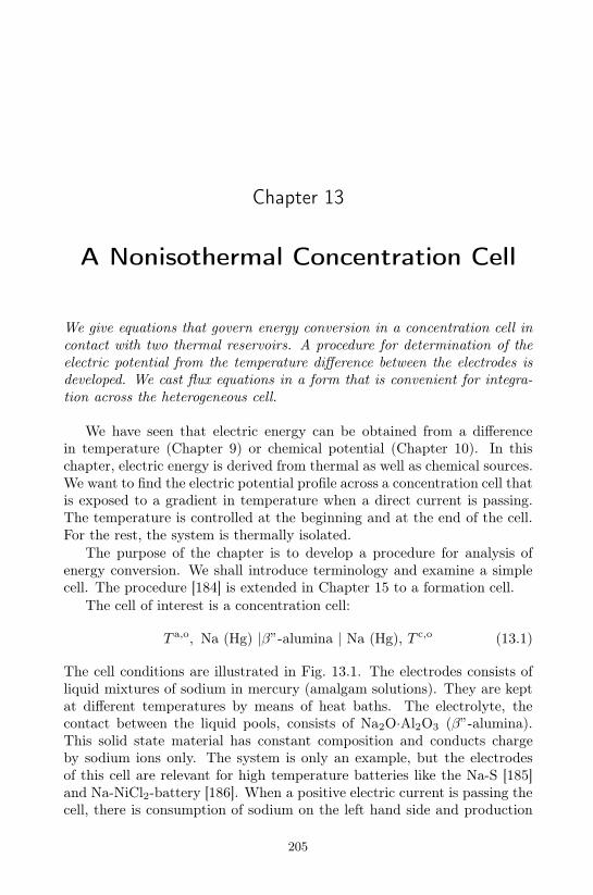
Chapter 13
A Nonisothermal Concentration Cell
We give equations that govern energy conversion in a concentration cell incontact with two thermal reservoirs. A procedure for determination of theelectric potential from the temperature difference between the electrodes isdeveloped. We cast flux equations in a form that is convenient for integra-tion across the heterogeneous cell.
We have seen that electric energy can be obtained from a differencein temperature (Chapter 9) or chemical potential (Chapter 10). In thischapter, electric energy is derived from thermal as well as chemical sources.We want to find the electric potential profile across a concentration cell thatis exposed to a gradient in temperature when a direct current is passing.The temperature is controlled at the beginning and at the end of the cell.For the rest, the system is thermally isolated.
The purpose of the chapter is to develop a procedure for analysis ofenergy conversion. We shall introduce terminology and examine a simplecell. The procedure [184] is extended in Chapter 15 to a formation cell.
The cell of interest is a concentration cell:
T a,o, Na (Hg) |β”-alumina | Na (Hg), T c,o (13.1)
The cell conditions are illustrated in Fig. 13.1. The electrodes consists ofliquid mixtures of sodium in mercury (amalgam solutions). They are keptat different temperatures by means of heat baths. The electrolyte, thecontact between the liquid pools, consists of Na2O·Al2O3 (β”-alumina).This solid state material has constant composition and conducts chargeby sodium ions only. The system is only an example, but the electrodesof this cell are relevant for high temperature batteries like the Na-S [185]and Na-NiCl2-battery [186]. When a positive electric current is passing thecell, there is consumption of sodium on the left hand side and production
205

206 Chapter 13. A Nonisothermal Concentration Cell
anode electrolyte cathode
anode surface cathode surface
−aluminaβNa(Hg) Na(Hg)
T
φ /
/K
V
a,o a,e e,a e,c c,as,cs,a
c,o
a,o a,e e,a
s,a
e,c c,a c,o
x/ m
x/ m
s,c
Figure 13.1 The temperature and electric potential profiles across the elec-trode concentration cell.
of sodium on the right hand side. The electric current leads to heatingof one electrode, and as we shall see, cooling of the other electrode. Suchreversible electrode heat effects have been studied in several systems thatare similar to the present cell [187]. Ito et al. [188] studied conditions duringwater electrolysis in hydroxide melts, Flem et al. [78,80] studied aluminiumelectrodes in contact with a fluoride mixture.
For pedagogical reasons, we start with the most general description.Relations between the variables will then appear (see Sec. 13.1.3).
The terminology used for electrochemical cells throughout the book isclarified in Figs. 13.1 and 13.2. At positions a,o and c,o in Fig. 13.1, thetemperatures are T a,o and T c,o and the electric potentials are φc,o andφa,o. A location is indicated by a superscript of two letters with a commabetween; the first letter refers to the phase, the second refers to the neigh-boring phase. The total cell potential, ∆totφ, between the end points is:
∆totφ = φc,o − φa,o = ∆aφ+ ∆a,eφ+ ∆eφ+ ∆e,cφ+ ∆cφ (13.2)

13.1. The homogeneous phases 207
Figure 13.2 Notation used for transport in electrochemical cells. The firstsymbol of a location (a superscript) refers to the phase, and the second to theneighbouring phase. A ∆ with one subscript, x, denotes the difference acrossphase x. A ∆ with two subscripts, x, y, denotes the value in y minus the valuein x.
The terminology in this equation is clarified in Fig. 13.2. The present cellhas five subsystems. From left to right we have: the anode, the anode sur-face, the electrolyte, the cathode surface and the cathode. There are threehomogeneous phases and two surfaces. When the electrodes are in contactwith different thermal reservoirs, the total potential is a thermoelectricpotential.
13.1 The homogeneous phases
We need expressions for T (x), µNa,T (x) and φ(x) between positions a,oand c,o in the presence of a current density, j, in order to find the ther-moelectric potential. One solution is illustrated in Fig. 13.1. We start theanalysis with the homogeneous phases, taking the anode as the detailedexample.
13.1.1 Entropy production and flux equations for the anode
The anode amalgam extends from position (a,o) to (a,e). Charge is con-ducted by electrons in the metal solution. A temperature gradient causessodium to move, leading in the stationary state to a Soret equilibrium

208 Chapter 13. A Nonisothermal Concentration Cell
for Na in Hg. Sodium must also be transported through the amalgamto supply the reaction at a,e. Heat is transported by conduction as wellas by charge and mass transport. The entropy production is therefore,cf. Eq. (4.15),
σa = J ′aq
(∂
∂x
1
T
)+ Ja
Na
(− 1
T
∂µaNa,T
∂x
)+ j
(− 1
T
∂φ
∂x
)(13.3)
where J ′aq is the measurable heat flux, Ja
Na the sodium flux and µaNa the
chemical potential of Na. The subscript T indicates that µaNa is differenti-
ated at constant temperature. The equations of transport are:
∂
∂x
1
T= Ra
qqJ′aq +Ra
qµJaNa +Ra
qφj
− 1
T
∂µaNa,T
∂x= Ra
µqJ′aq +Ra
µµJaNa +Ra
µφj
− 1
T
∂φ
∂x= Ra
φqJ′aq +Ra
φµJaNa +Ra
φφj
(13.4)
It will also be convenient to express the fluxes in the forces
J ′aq = La
∂
∂x
1
T+ La
qµ
(− 1
T
∂µaNa,T
∂x
)+ La
qφ
(− 1
T
∂φ
∂x
)
JaNa = La
µq
∂
∂x
1
T+ La
µµ
(− 1
T
∂µaNa,T
∂x
)+ La
µφ
(− 1
T
∂φ
∂x
)
j = Laφq
∂
∂x
1
T+ La
φµ
(− 1
T
∂µaNa,T
∂x
)+ La
φφ
(− 1
T
∂φ
∂x
)(13.5)
The conductivity matrix is the inverse of the resistivity matrix and can befound using Kramers’ rule, see Sec. 7.4. Resistivities as well as conductivi-ties satisfy the Onsager relations.
We are looking for expressions where T (x), µNa,T (x) and φ(x) are givenin terms of measured transport properties, and continue to rewrite thelinear relations between the fluxes and forces. We solve for ∂φ/∂x fromEq. (13.5c) and eliminate this gradient in Eq. (13.5a, b). The result is
J ′aq = laqq
∂
∂x
1
T+ laqµ
(− 1
T
∂µaNa,T
∂x
)+πa
Fj
JaNa = laµq
∂
∂x
1
T+ laµµ
(− 1
T
∂µaNa,T
∂x
)+taNa
Fj
∂φ
∂x= − πa
TF
∂T
∂x− taNa
F
∂µaNa,T
∂x− raj
(13.6)
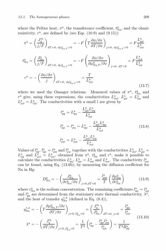
13.1. The homogeneous phases 209
where the Peltier heat, πa, the transference coefficient, taNa, and the ohmicresistivity, ra, are defined by (see Eqs. (10.9) and (9.15)):
πa =
(J ′a
q
j/F
)
dT=0, dµaNa,T
=0
= −F(T∂φ/∂x
∂T/∂x
)
j=0, dµaNa,T
=0
= FLa
qφ
Laφφ
taNa =
(Ja
Na
j/F
)
dT=0, dµaNa,T
=0
= −F(
∂φ/∂x
∂µaNa,T /∂x
)
j=0, dT=0
= FLa
µφ
Laφφ
ra = −(∂φ/∂x
j
)
dT=0, dµaNa,T
=0
=T
Laφφ
(13.7)
where we used the Onsager relations. Measured values of πa, taNa andra give, using these expressions, the conductivities La
φφ, Laqφ = La
φq andLa
µφ = Laφµ. The conductivities with a small l are given by
laqq = Laqq −
LaqφL
aφq
Laφφ
laqµ = laµq = Laqµ −
LaqφL
aφµ
Laφφ
laµµ = Laµµ −
LaµφL
aφµ
Laφφ
(13.8)
Values of laqq, laqµ = laµq and laµµ together with the conductivities La
φφ, Laqφ =
Laφq and La
µφ = Laφµ, obtained from πa, taNa and ra, make it possible to
calculate the conductivities Laqq, L
aqµ = La
µq and Laµµ. The conductivity laµµ
can be found, using Eq. (13.6b), by measuring the diffusion coefficient forNa in Hg:
DaNa = −
(Ja
Na
∂caNa/∂x
)
j=0,dT=0
=laµµ
T
(∂µa
Na
∂caNa
)(13.9)
where caNa is the sodium concentration. The remaining coefficients laqµ = laµq
and laqq are determined from the stationary state thermal conductivity, λa,and the heat of transfer q∗,a
Na (defined in Eq. (8.4)),
q∗,aNa = −
(T∂µa
Na,T /∂x
∂T/∂x
)
j=0,JaNa
=0
=
(J ′a
q
JaNa
)
dT=0, j=0
=laqµ
laµµ
λa = −(
J ′aq
∂T/∂x
)
j=0,JaNa
=0
=1
T 2
(laqq −
laqµlaµq
laµµ
)=
1
T 2Raqq
(13.10)

210 Chapter 13. A Nonisothermal Concentration Cell
This gives a practical form of the linear force-flux relations:
∂T
∂x= − 1
λa
[J ′a
q − q∗,aNa
(Ja
Na −taNa
Fj
)− πa
Fj
]
∂µaNa,T
∂x= −q
∗,aNa
T
∂T
∂x− T
laµµ
(Ja
Na −taNa
Fj
)
∂φ
∂x= − πa
TF
∂T
∂x− taNa
F
∂µaNa,T
∂x− raj
(13.11)
The profiles we are seeking are expressed in terms of measurable transportproperties. The expressions above defined the measurements to find thecoupling coefficients πa, taNa and q∗,a
Na , and the diagonal coefficients ra, DaNa
and λa. Knowledge of these coefficients makes it possible to solve theexpressions above.
13.1.2 Position dependent transport coefficients
We shall see that the boundary conditions for the sodium flux leads to aposition dependent transference coefficient of Na in amalgam.
The transference coefficient is defined as the flow of sodium to the site ofthe electrode reaction, caused by the constant electric current, for a positionindependent temperature, chemical potential, or concentration of sodium;i.e. caNa(x, t) = caNa(t). The ratio of the two fluxes varies from position 0 atthe iron contact to position da at the electrode surface, because the sodiumflux varies across the electrode at these conditions. This can be found fromthe mass balance for sodium:
∂caNa(x, t)
∂t= −∂J
aNa(x, t)
∂x(13.12)
The flux of Na that is leaving the electrode, is given by the integral:
∂
∂t
∫ da
0
caNadx = −JaNa(d
a, t) + JaNa(0, t) = −Ja
Na(da, t) = − j
F(13.13)
The sodium flux is zero at position 0, and equal to j/F at position da. Theelectric current is independent of the position and the time. We now use thedefinition of the transference coefficient, Eq. (13.7b). When the gradientsof the concentration and temperature are zero, Ja
Na(x, t) = taNa(x, t)j/F,and we have
∂caNa(t)
∂t= −∂J
aNa(x, t)
∂x= − j
F
∂taNa(x, t)
∂x= − j
daF(13.14)

13.1. The homogeneous phases 211
The solutions for JaNa(x, t)and tNa(x, t) are therefore
JaNa(x, t) =
xj
daF→ taNa(x, t) =
x
da(13.15)
Both solutions are time independent. The concentration of sodium is slowlydecreasing, however. The solution is in that sense only quasi-stationary.But the transference coefficient has been found to be time independent,and to increase linearly from 0 at the metal contact to 1 at the electrodesurface.
The Peltier coefficient is also position dependent. This dependencycan be derived using the expression for the measurable heat flux, J ′a
q =T (Js − JNaS
aNa), cf. Eq. (4.12). By introducing this into Eq. (13.7a) we
have
πa(x) =
(J ′a
q
j/F
)
dT=0, dµaNa,T =0
= T
(Js − JNaS
aNa
j/F
)
dT=0, dµaNa,T =0
= −T [S∗e− + taNa(x)S
aNa] (13.16)
where S∗e− is by definition the transported entropy of the electrons
(cf. Chapter 9).
Remark 13.1. As the position dependence of taNa and πa shows, thesequantities are not just material properties. They also depend on the bound-ary conditions, see also Ref. [189].
Remark 13.2. The entropy and the transported entropy are functions ofthe temperature and other intensive variables that characterize the localthermodynamic state. We have neglected such dependencies here.
13.1.3 The profiles of the homogeneous anode
We can now obtain some relations between the variables. The heat oftransfer can be determined from the expression for the electric potentialgradient in Eq. (13.11), when JNa and j are zero. This gives
∂φ
∂x=
1
F
[S∗
e− + taNa(x)
(Sa
Na +q∗,aNa
T
)]∂T
∂x(13.17)
The electric potential gradient cannot depend on the position dependenttransference number. It follows that the transported heat is:
q∗,aNa = −TSa
Na (13.18)

212 Chapter 13. A Nonisothermal Concentration Cell
For small fluxes, we can expect that the sodium flux is a linear functionof the position. The boundary conditions then give Ja
Na(x) = taNa(x)j/F =xj/daF . This further simplifies Eq. (13.11) considerably. After some alge-bra, we obtain
∂T
∂x= − 1
λa
[J ′a
q − πa j
F
]= − 1
λa
[J ′a
q + T(S∗
e− +x
daSa
Na
) j
F
]
∂µaNa,T
∂x= Sa
Na
∂T
∂x→ ∂µa
Na
∂x= 0
∂φ
∂x=S∗
e−
F
∂T
∂x− raj
(13.19)
The equations say that true equilibrium is established for Na across theelectrode, as ∂µa
Na/∂x = 0. The electric potential drop consists of an ohmicpotential drop, plus a contribution from the temperature difference. Theheat transport has, likewise, also two contributions. The derivation inSec. 13.1.1 may seem cumbersome, but it is important to take all termsalong to find the condition of chemical equilibrium Eq. (13.19b). In asimpler analysis, one could introduce in the entropy production, Ja
Na(x) =xj/daF , to give two forces and fluxes directly. While this appears to besimpler, it may hide the relation q∗,a
Na = −TSaNa and the condition for a
constant chemical potential of the sodium.
13.1.4 Contributions from the cathode
The formulae are the same for the cathode and the anode, but the boundaryconditions differ. The sodium flux is j/F at position da + de (the cathodesurface) and 0 at the position of the metal contact, da + de + dc. Thetransference coefficient is therefore
tcNa(x) = 1 − x− da − de
dc(13.20)
The Peltier coefficient and the heat of transport are, cf. Eqs. (13.16) and(13.18),
πc = −T [S∗e− + tcNa(x)S
cNa] and q∗,c
Na = −TScNa (13.21)
The rest of the equations are similar to the ones written for the anode.Analogous to Eq. (13.19) we find

13.1. The homogeneous phases 213
∂T
∂x= − 1
λc
J ′c
q + T
[S∗
e− +
(1 − x− da − de
dc
)Sc
Na
]j
F
∂µcNa,T
∂x= Sc
Na
∂T
∂x→ ∂µc
Na
∂x= 0
∂φ
∂x=S∗
e−
F
∂T
∂x− rcj
(13.22)
Integration is now easy. In Fig. 13.1, ∆cφ is negative. This corresponds toT c,e > T c,o.
13.1.5 The electrolyte contribution
The entropy production in the non-isothermal electrolyte of β”-alumina is
σe = J ′eq
∂
∂x
(1
T
)+ j
[− 1
T
∂φ
∂x
](13.23)
The flux equations are
∂
∂x
(1
T
)= Re
qqJ′eq +Re
qφj
− 1
T
∂φ
∂x= Re
φqJ′eq +Re
φφj
(13.24)
or alternatively,
J ′eq = Le
qq∂∂x
(1
T
)+ Le
qφ
(− 1
T
∂φ
∂x
)
j = Leφq
∂
∂x
(1
T
)+ Le
φφ
(− 1
T
∂φ
∂x
) (13.25)
The Peltier coefficient for the electrolyte is:
πe =
(J ′e
q
j/F
)
dT=0
= −FRe
qφ
Reqq
= FLe
qφ
Leφφ
= TS∗Na+ (13.26)
The stationary state thermal conductivity and the ohmic resistivity aregiven by:
λe =1
T 2Reqq
and re =T
Leφφ
(13.27)

214 Chapter 13. A Nonisothermal Concentration Cell
The flux equations can then be written
∂T
∂x= − 1
λe
(J ′e
q − πe j
F
)= − 1
λe
(J ′e
q − TS∗Na+
j
F
)
∂φ
∂x= − πe
TF
∂T
∂x− rej = − 1
FS∗
Na+
∂T
∂x− rej
(13.28)
where the Onsager relation has been used. The electric potential differenceacross the electrolyte is linear in the temperature difference. The sign of∆eφ is negative in Fig. 13.1. This corresponds to a temperature increaseacross the electrolyte from the anode to the cathode and an ohmic potentialdrop.
13.2 Surface contributions
13.2.1 The anode surface
This surface has the position (s,a) in Figs. 13.1 and 13.2. After sodiumarrives at the anode surface, the reaction is:
Na(a) → Na+(e) + e−(a) (13.29)
The electron is subsequently transferred to the conduction band in themetal, and the sodium ion is transferred to the β′′-alumina. The contribu-tion from the sodium to the reaction Gibbs energy is
∆nGs,a = −µs,a
Na = −µs,aNa (T s,a) (13.30)
The entropy production in the non-isothermal anode surface becomes,cf. Eq. (5.15):
σs,a = J ′a,eq
(∆a,s
1
T
)+ J ′e,a
q
(∆s,e
1
T
)− Ja,e
Na
∆a,sµNa,T (T s,a)
T s,a
− j∆a,eφ
T s,a− r
∆nGs,a
T s,a(13.31)
For stationary state conditions the sodium flux is equal to the reaction rate,which is equal to j/F . This gives
−Ja,eNa
∆a,sµNa,T (T s,a)
T s,a− r
∆nGs,a
T s,a=
j
F
µa,eNa (T s,a)
T s,a(13.32)
We introduce this expression in Eq. (13.31) and obtain
σs,a = J ′a,eq
(∆a,s
1
T
)+ J ′e,a
q
(∆s,e
1
T
)− j
(∆a,eφ− µa,e
Na (T s,a) /F
T s,a
)
(13.33)

13.2. Surface contributions 215
By taking along all fluxes, like we did in the bulk anode, we find that thechemical potential at the surface, µs,a
Na, is equal to the constant chemicalpotential in the anode, µa
Na.We next assume, as explained in Chapter 8, that the inverse temperature
differences from one side of the surface do not couple to the measurable heatfluxes on the other side, see also Sec. 9.2. This gives
∆a,s
(1
T
)= Rs,a
qq J′a,eq +Rs,a
qφ j
∆s,e
(1
T
)= Rs,e
qq J′e,aq +Rs,e
qφj
− 1
T s,a
(∆a,eφ− µa,e
Na (T s,a)
F
)= Rs,a
φqJ′a,eq +Rs,e
φqJ′e,aq +Rs,a
φφj
(13.34)
The resistivities satisfy the Onsager relations. The relations for both sidesof the surface may be written in a form similar to Eq. (13.11)
∆a,sT = − 1
λs,a
(J ′a,e
q − πa,e j
F
)
∆s,eT = − 1
λs,e
(J ′e,a
q − πe,a j
F
)
∆a,eφ− 1
Fµa,e
Na (T s,a) = − πa,e
T a,eF∆a,sT − πe,a
T e,aF∆s,eT − rs,aj
(13.35)
where the coefficients are now given by
πa,e =
(J ′a,e
q
j/F
)
∆a,sT=0
= −FRs,a
qφ
Rs,aqq
πe,a =
(J ′e,a
q
j/F
)
∆s,eT=0
= −FRs,e
qφ
Rs,eqq
λs,a =1
Rs,aqq T s,aT a,e
and λs,e =1
Rs,eqq T s,aT e,a
rs,a = T s,a
(Rs,a
φφ −Rs,a
qφRs,aφq
Rs,aqq
−Rs,e
qφRs,eφq
Rs,eqq
)
(13.36)
The transport properties πa,e and πe,a are ratios of fluxes in homogeneousphases, and are therefore equal for the surface and the adjacent homoge-neous phase. The coefficient πe, defined in the previous section, expresses

216 Chapter 13. A Nonisothermal Concentration Cell
that the charge transport by sodium ion leads to heat transport away fromthe anode surface. Using Eqs. (13.16) and the analogous relation in theelectrolyte, we have
πa,e = −T a,e (S∗e− + Sa,e
Na) and πe,a = −T e,aS∗Na+ (13.37)
where S∗Na+ is the transported entropy of the sodium ion in the β′′-alumina.
Substituting these relations in Eq. (13.35) gives
∆a,sT = − 1
λs,a
(J ′a,e
q + T a,e (S∗e− + Sa,e
Na)j
F
)
∆s,eT = − 1
λs,e
(J ′e,a
q + T e,aS∗Na+
j
F
)
∆a,eφ− 1
Fµa,e
Na (T s,a) =1
F(S∗
e− + Sa,eNa) ∆a,sT +
1
FS∗
Na+∆s,eT − rs,aj
(13.38)
Using µa,eNa (T s,a) = µa
Na − Sa,eNa∆a,sT = µs,a
Na − Sa,eNa∆a,sT the relation for the
electric potential reduces to
∆a,eφ− 1
Fµs,a
Na =1
FS∗
e−∆a,sT +1
FS∗
Na+∆s,eT − rs,aj (13.39)
In Fig. 13.1, ∆a,eφ is positive. This is consistent with the negative reactionGibbs energy (a tendency for Na to react) and a decrease in temperatureacross the surface.
The above results now show that the expressions for the surface are nat-ural prolongations of the expressions for the homogeneous phases. They aresimplified because there is no sodium adsorption at the surface. The simi-larity in the description of the homogeneous regions and the surface makesit simple to integrate across the heterogeneous system. The Peltier heatson both sides of the surface were equal to their values in the homogeneousphases. Only three new coefficients are needed to describe the surface, λs,a,λs,e and rs,a.
Remark 13.3. The Nernst equation for the surface in its two equivalentformulations is
∆a,eφ+1
F∆nG
s,a = ∆a,eφ− 1
Fµs,a
Na = ∆a,eψ +1
F
(µa,e
e−+ µe,a
Na+ − µs,aNa
)
≡ ∆a,eψ +1
F∆rG
s,a = 0 (13.40)

13.2. Surface contributions 217
and the total cell potential is
∆totφ = ∆aψ + ∆a,eψ + ∆eψ + ∆e,cψ + ∆cψ
+1
F(∆rG
s,a + ∆rGs,c) − 1
F(µa,e
Na − µc,eNa) (13.41)
13.2.2 The cathode surface
We can now write, by direct analogy, the equations of interest for the cath-ode surface. The surface has the position (s,c) in Figs. 13.1 and 13.2. Thesodium ion and the electron are transported to the anode surface and reactaccording to:
Na+(e) + e−(c) → Na(c) (13.42)
The contribution from the sodium to the reaction Gibbs energy is
∆nGs,c = µs,c
Na = µs,cNa (T s,c) (13.43)
where the reaction rate is equal to j/F. The entropy production rate and theflux equations follow in a similar manner as for the anode. The equationsto be solved are analogous to Eq. (13.35).
∆e,sT = − 1
λs,e
[J ′e,c
q − πe,c j
F
]
∆s,cT = − 1
λs,c
[J ′c,e
q − πc,e j
F
]
∆e,cφ+1
Fµc,e
Na (T s,c) = − πe,c
T e,cF∆e,sT − πc,e
T c,eF∆s,cT − rs,cj
(13.44)
where we added the electric potential differences. Using Eqs. (13.16),(13.26) and (13.43), for the cathode surface gives
∆e,sT = − 1
λs,e
(J ′e,c
q + T e,cS∗Na+
j
F
)
∆s,cT = − 1
λs,c
(J ′c,e
q + T c,e(S∗
e− + Sc,eNa
) jF
)
∆e,cφ+1
Fµs,c
Na =1
FS∗
Na+∆e,sT +1
FS∗
e−∆s,cT − rs,cj
(13.45)
which is the analogue of Eq. (13.38). The chemical potential of sodium inthe cathode is constant and equal to the chemical potential at the cathodesurface. This is similar to in the anode.
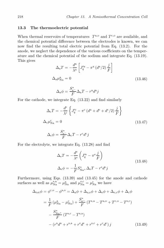
218 Chapter 13. A Nonisothermal Concentration Cell
13.3 The thermoelectric potential
When thermal reservoirs of temperatures T a,o and T c,o are available, andthe chemical potential difference between the electrodes is known, we cannow find the resulting total electric potential from Eq. (13.2). For theanode, we neglect the dependence of the various coefficients on the temper-ature and the chemical potential of the sodium and integrate Eq. (13.19).This gives
∆aT = − da
λa
[J ′a
q − πa (da/2)j
F
]
∆aµaNa = 0
∆aφ =S∗
e−
F∆aT − radaj
(13.46)
For the cathode, we integrate Eq. (13.22) and find similarly
∆cT = − dc
λc
J ′c
q − πc (da + de + dc/2)j
F
∆cµcNa = 0
∆cφ =S∗
e−
F∆cT − rcdcj
(13.47)
For the electrolyte, we integrate Eq. (13.28) and find
∆eT = − de
λe
(J ′e
q − πe j
F
)
∆eφ = − 1
FS∗
Na+∆eT − redej
(13.48)
Furthermore, using Eqs. (13.39) and (13.45) for the anode and cathodesurfaces as well as µs,a
Na = µaNa and µs,c
Na = µcNa we have
∆totφ = φc,o − φa,o = ∆aφ+ ∆a,eφ+ ∆eφ+ ∆e,cφ+ ∆cφ
=1
F(µa
Na − µcNa) +
S∗e−
F(T s,a − T a,o + T c,o − T s,c)
−S∗
Na+
F(T s,c − T s,a)
− (rada + rs,a + rede + rs,c + rcdc) j (13.49)

13.3. The thermoelectric potential 219
The expressions for all the temperature differences (13.46), (13.47), and(13.48), and the electrode potentials, Eqs. (13.38) and (13.45), give the con-version between thermal, chemical and electric energy in the cell. Kjelstrupand Bedeaux [130] calculated the corresponding profiles of temperature andelectric potential in the solid oxide fuel cell. Kjelstrup et al. calculated thepresent cell [184].

This page intentionally left blankThis page intentionally left blank

Chapter 14
The Transported Entropy
We describe how the transported entropy can be determined by measuringthe Seebeck coefficient of an electrochemical cell. Selected values of thetransported entropies are presented. The transported entropies obey certaintransformation properties, because potential differences and the electric cur-rent density are independent of the frame of reference.
We saw in Chapters 8 and 13, that the conversion from thermal to elec-tric energy, or vice versa, depended on the magnitude of the transportedentropies in conductors of the system. For electronic conductors, this quan-tity is normally not large, typically a few J/K mol [153,190]. This seriouslylimits the efficiency of thermal energy conversion. By using ions as chargecarriers instead of electrons, attempts have been made to find cells withlarger thermoelectric powers. Large Peltier coefficients have been found incells with complex formations [78,191] and with gas electrodes [192].
Systematic knowledge about transported entropies has been gathered byAgar [148,193]. The purpose of this chapter is to describe how transportedentropies can be determined, which relations they must obey, and what theirproperties are. We describe how transported entropies can be obtained frommeasurements in three example cells:
T l, Mo(s)|Pb(l)|PbCl2(l), MCl(l)|Pb(l)|Mo(s), T r (a)
T a, M(Hg)|β′′-alumina|M(Hg), T c (b)
T l, Ag(s)|AgCl(s)|MCl(aq)|AgCl (s)|Ag(s), T r (c)
Cell a has electrodes of liquid lead, and an electrolyte mixture of two moltensalts. The liquid lead pools are connected to the potentiometer via molyb-denum wires [194]. Cell b was described in Chapter 13 with M = Na [195].Cell c has an aqueous electrolyte [196], and shall be further discussed in
221

222 Chapter 14. The Transported Entropy
Chapter 15. The metal contacts to the cells a and c are thermostatted attemperatures T l and T r. In cell b, they are thermostatted to T a and T c
respectively.
14.1 The Seebeck coefficient of cell a
Cell a has five homogeneous phases and four interfaces. The homogeneousphases are denoted l, a, e, c and r, respectively. The surfaces between themare denoted (s,l), (s,a), (s,c) and (s,r).
The chemical reaction on the electrodes takes half a mole of lead fromthe anode surface
1
2Pb → 1
2Pb2+ + e− (14.1)
and adds the same amount to the cathode surface when a faraday of chargeis passed through the cell. For a positive electric current density j boththe (s,a) and the (s,c) surface move to the left relative to the (s,l) andthe (s,r) surfaces, with a small velocity proportional to j. The ions of thetwo salts move in the electrolyte. Chemical potential gradients of the saltsdevelop in a temperature gradient after a few hours. We are interested inthe state when the chemical potential gradient of PbCl2 produced by thenon-zero electric current density is balanced by the thermal force, that is,in the Soret equilibrium. In this state, there is no transport of PbCl2 orMCl relative to the (s,a) and the (s,c) surfaces. We will show that one canthen find the transported entropy of lead ions in a simple way.
The entropy production in the metal phases is
σ = J ′q
(∂
∂x
1
T
)+ j
(− 1
T
∂φ
∂x
)(14.2)
The equations for the temperature gradient and the electric potential gra-dient are the same as derived in Sec. 9.1
∂T
∂x= − 1
λ
(J ′
q − πj
F
)
∂φ
∂x= − π
TF
∂T
∂x− rj
(14.3)
The Peltier coefficients for the solid Mo phases and for the lead pools are:
πl = πr = TS∗e−,Mo and πa = πc = TS∗
e−,Pb (14.4)

14.1. The Seebeck coefficient of cell a 223
Neglecting the variation of the coefficients λ, r, π, S∗e−,Mo
, S∗e−,Pb
with thetemperature, the equations give for the molybdenum phases:
∆lT = − dl
λl
(J ′l
q − πl j
F
)and ∆lφ = − 1
FS∗
e−,Mo∆lT − rldlj
∆rT = − dr
λr
(J ′r
q − πr j
F
)and ∆rφ = − 1
FS∗
e−,Mo∆rT − rrdrj
(14.5)and for the lead phases:
∆aT = − da
λa
(J ′a
q − πa j
F
)and ∆aφ = − 1
FS∗
e−,Pb∆aT − radaj
∆cT = − dc
λc
(J ′c
q − πc j
F
)and ∆cφ = − 1
FS∗
e−,Pb∆cT − rcdcj
(14.6)
The molybdenum-lead interfaces were described in Sec. 9.2. The poten-tial drops across these interfaces were, cf. Eq. (9.18):
∆l,aφ = − 1
FS∗
e−,Mo
(T s,l − T l,a
)− 1
FS∗
e−,Pb
(T a,l − T s,l
)− rs,lj
∆c,rφ = − 1
FS∗
e−,Pb(T s,r − T c,r) − 1
FS∗
e−,Mo(T r,c − T s,r) − rs,rj
(14.7)
The entropy production of the interface has a similar structure as inSec. 13.2. For the lead-electrolyte interface, we have in a frame of referencethat moves along with the surface
σs,a = J ′aq
(∆a,s
1
T
)+ J ′e
q
(∆s,e
1
T
)+ j
[− 1
T s,a
(∆a,eφ+
∆nGs,a
F
)]
(14.8)
The reaction rate is proportional to the electric current density, rs = j/F ,and so is the transport of Pb into the surface, Ja
Pb = j/2F . The contributionto the reaction Gibbs energy from the neutral components is ∆nG
s,a =−µa,e
Pb (T s,a) /2. As the quantities of interest do not depend on the chosenframe of reference, we may use a different frame of reference than the oneused above. The linear relations are, using the same approximations as in

224 Chapter 14. The Transported Entropy
Sec. 9.2,
∆a,sT = − 1
λs,aaa
(J ′a
q − πa j
F
)
∆s,eT = − 1
λs,aee
(J ′e
q − πe j
F
)
∆a,eφ− 1
2Fµa,e
Pb = − 1
FS∗
e−,Pb∆a,sT − 1
2FS∗,e
Pb2+∆s,eT − rs,aj
(14.9)
where rs,a is the ohmic resistivity of the surface. The Peltier coefficients onthe anode and cathode sides were given in Eq. (14.4). The Peltier coefficientin the electrolyte
πe =1
2T eS∗,e
Pb2+ (14.10)
expresses that the stationary state charge transport by lead ions gives heattransport away from the surface corresponding to one equivalent of leadion.
For the electrolyte-lead surface we find similarly
∆e,sT = − 1
λs,cee
(J ′e
q − πe j
F
)
∆s,cT = − 1
λs,cee
(J ′c
q − πc j
F
)
∆e,cφ+1
2Fµc,e
Pb = − 1
2FS∗,e
Pb2+∆e,sT − 1
FS∗
e−,Pb∆s,cT − rs,cj
(14.11)
The entropy production of the electrolyte has four terms
σ = J ′q
(∂
∂x
1
T
)+ JPbCl2
(− 1
T
∂µPbCl2,T
∂x
)
+ JMCl
(− 1
T
∂µMCl,T
∂x
)+ j
(− 1
T
∂φ
∂x
)(14.12)
We will again use the frame of reference in which the electrode-electrolytesurfaces are not moving. We are interested in the stationary state whenJMCl and JPbCl2 are zero. Only two terms then remain in the entropyproduction, and we obtain the same transport equations as those found forthe molybdenum wires and the lead pools:
∆eT = − de
λe
(J ′e
q − πe j
F
)
∆eφ = − 1
2FS∗,e
Pb2+∆eT − redej
(14.13)

14.1. The Seebeck coefficient of cell a 225
All coefficients refer to the stationary state in question. This means thatthe resistivity, for instance, is the resistivity of a mixture with salt andgradients, which was assumed to be constant in Eq. (14.13). The stationarystate Peltier coefficient for the electrolyte is given in Eq. (14.10).
The total cell potential is now obtained by adding all contributions
F∆totφ = F (∆lφ+ ∆l,aφ+ ∆aφ+ ∆a,eφ+ ∆eφ+ ∆e,cφ
+ ∆cφ+ ∆c,rφ+ ∆rφ)
= −1
2[µc,e
Pb (T s,c) − µa,ePb (T s,a)] +
(S∗
e−,Mo − S∗e−,Pb
) (T s,r − T s,l
)
+
(S∗
e−,Pb − 1
2S∗,e
Pb2+
)(T s,c − T s,a)
−(rldl + rs,l + rada + rs,a + rede + rs,c + rcdc + rs,r + rrdr
)jF
= −1
2[Hc,e
Pb (T s,c) −Ha,ePb (T s,a)] +
(S∗
e−,Mo − S∗e−,Pb
) (T s,r − T s,l
)
+
(S∗
e−,Pb − 1
2
(S∗,e
Pb2+ − SPb
))(T s,c − T s,a)
−(rldl + rs,l + rada + rs,a + rede + rs,c + rcdc + rs,r + rrdr
)jF
(14.14)
where we used the assumption that the temperatures on both sides of thepotentiometer are equal, i.e. T l,o = T r,o. Contributions due to the tem-perature dependence of the entropies and the ohmic resistivities have beenneglected.
When the two electrode pools are thermostatted at T s,l = T a,l = T a,e =T s,a ≡ T a and T s,c = T c,e = T c,r = T s,r ≡ T c, the electric current iszero, and if one neglects the temperature dependence of the enthalpy, theexpression reduces to
F∆totφ =
[S∗
e−,Mo −1
2
(S∗,e
Pb2+ − SPb
)](T c − T a) (14.15)
The Seebeck coefficient can thus be defined as
ηS =
(∆totφ
∆T
)
j=0
=1
F
[S∗
e−,Mo −1
2
(S∗,e
Pb2+ − SPb
)](14.16)

226 Chapter 14. The Transported Entropy
Table 14.1 The transported entropy of Pb2+ at 798 K [194].
MCl xPbCl2 ηS,1 / µV K−1 S∗Pb2+ / J mol−1 K−1
LiCl 0.7 4.8 1030.5 8.9 106
NaCl 0.8 15.2 1010.57 8.1 102
KCl 0.68 23.8 1000.54 21.0 100
RbCl 0.8 23.4 1000.5 32.4 102
CsCl 0.6 23.9 99– 1 −10.1 102
The electric potential difference can be measured with good accuracy, andso can the temperature difference. The ratio gives a possibility for anaccurate determination of S∗,e
Pb2+ [194]. The alternative, to determine thetransported entropy from the Peltier heat, is less accurate.
The cell in this section was described under stationary state conditions,when the salt fluxes are zero. The more general case was described fordifferent systems by Grimstvedt et al. [197] and Flem et al. [80].
14.2 The transported entropy of Pb2+ in cell a
The Seebeck coefficient of cell a is according to the above derivations:
ηS,1 =1
F
(S∗
e−,Mo −1
2S∗,e
Pb2+ +1
2SPb
)(14.17)
The corresponding expression for the cell of Sec. 9.1 was
ηS,2 =1
F
(S∗
e−,Mo − S∗e−,Pb
)(14.18)
Their difference was used to find the properties of lead ion
ηS,1 − ηS,2 =1
F
(S∗
e−,Pb − 1
2S∗
Pb2+ +1
2SPb
)(14.19)

14.3. The transported entropy of the cation in cell b 227
The Seebeck coefficient for Mo(s)|Pb(l)| Mo(s) is ηS,2 = 20.6 µV/K.The coefficient for main cell is, ηS,1, with pure PbCl2 is −10.1 µV/K at 798K. We use the transported entropy of electrons in lead as a reference, i.e.S∗
e−,Pb≡ 0. The transported entropy S∗,e
Pb2+ in pure PbCl2 is then foundto be 102 J/mol K. Some selected values for electrolyte mixtures are givenin Table 14.1 [194]. Surprisingly, the transported entropy of lead variesonly very little, from 99 to 106, as the cation M+ is exchanged or as thecomposition changes.
14.3 The transported entropy of the cation in cell b
We saw in Chapter 13 that the total cell potential of cell b (with M = Na)was:
∆totφ− 1
F(µa,e
Na − µc,eNa) = ∆aφ+ ∆a,eφ+ ∆eφ+ ∆e,cφ+ ∆cφ
− 1
F(µa,e
Na − µc,eNa)
=S∗
e−
F(T a,e − T c,e) −
S∗Na+
F(T e,c − T e,a)
− (rada + rs,a + rs,e + rede + rs,e + rs,c + rcdc) j
(14.20)
The electrodes, including their surfaces, are thermostatted at temperaturesT a and T c [198]. This means that T a,e = T s,a = T e,a = T a and T e,c =T s,c = T c,e = T c. The potentiometer is at temperature T a,o = T c,o ≡ T o.The potential difference becomes:
(∆totφ)j→0 =1
F
(SNa + S∗
e− − S∗Na+
)(T c − T a) (14.21)
The Seebeck coefficient for a cell with a metal M is therefore
ηS =1
F
(SM − S∗
M+ + S∗e−
)(14.22)
Only the combination of the transported entropy of the M+-ions in the β′′-alumina and of the electrons in the iron can be obtained from the Seebeck-coefficient. In order to allocate a value to a single charge carrier, a referencemust be chosen. It is customary to use the transported entropy in lead (Pb)as a zero reference [27]. The transported entropy of electrons in Fe then, issmall and positive, 1 J/K mol.

228 Chapter 14. The Transported Entropy
Table 14.2 The transported entropy of cations in selected materials [198].
Material Conducting Transported entropy
ion / J K−1 mol−1
Na-β′′-alumina Na+ 60 ± 5
K-β′′-alumina K+ 60 ± 3
Ag-β′′-alumina Ag+ 57 ± 5
NaF Na+ 81 ± 8
Na3AlF6 Na+ 140 ± 7
Results for Na+, obtained from such measurements, are listed inTable 14.2 together with results for some other ions.
14.4 The transported entropy of the ions cell c
The total cell potential of cell c, when operated at stationary state con-ditions, can be found by adding all contributions of the separate parts, aswill be described in more detail in Chapter 15:
∆φ = ∆l,aφ+ ∆aφ+ ∆a,eφ+ ∆eφ+ ∆e,cφ+ ∆cφ+ ∆c,rφ
= − 1
F
(µr,c
Ag − µl,aAg
)+
1
F
(µc,e
AgCl − µa,eAgCl
)
+1
F(S∗
e− − SAg) (∆l,sT + ∆s,rT )
− 1
FS∗
Ag+
(T s,r − T s,c + T s,a − T s,l
)
+1
FSAgCl (∆a,sT + ∆s,cT ) +
1
FS∗
Cl− (T s,c − T s,a)
−(rs,l + rada + rs,a + rede + rs,c + rcdc + rs,r
)j (14.23)
Again, we took all thermodynamic properties and all transported entropiesindependent of the temperature. By introducing the expression for thechemical potentials and neglecting the temperature dependence of the

14.4. The transported entropy of the ions cell c 229
enthalpies, we obtain
∆φ =1
F
(T s,r − T s,l
)SAg −
1
FS∗
Ag+
(T s,r − T s,c + T s,a − T s,l
)
− 1
FS∗
e− (∆l,sT + ∆s,rT ) − 1
FSAgCl (T
s,c − T s,a)
+1
FS∗
Cl− (T s,c − T s,a)
−(rs,l + rada + rs,a + rede + rs,c + rcdc + rs,r
)j (14.24)
In the thermostatted cell the surfaces of the electrodes, where the electro-chemical reactions take place, are thermostatted. Consider therefore thecase that all solid state parts of the electrode, including the adjacent elec-trolyte layer, are thermostatted. The temperature is T a on the anode sideand T c on the cathode side. Using Eq. (14.24) for zero electric current oneobtains:
∆φ =1
F
(SAg − SAgCl + S∗
e− + S∗Cl−
)(T c − T a) (14.25)
The Seebeck coefficient for the cell in stationary state is
ηS =
(∆φ
T c − T a
)=
1
F
[SAg − SAgCl + S∗
e− + S∗Cl−
](14.26)
A determination of the slope of the plot of the experimental ∆φ versus(T c−T a) allows us to determine S∗
Cl−+S∗
e− when thermodynamic entropiesof Ag and AgCl are known. At 298 K, SAg = 42.7 J/K mol and SAgCl = 96.2J/K mol. These values were used, and the results for S∗
Cl−are given in
Table 14.3 [196]. The transported entropy of electrons was neglected. Thetransported entropy for chloride ions is relatively constant as a functionof composition (apart from that in HCl(aq)). This is similar to the resultfound for Pb2+ in Sec. 14.2.
By taking along also MCl as a component, and defining the heat oftransfer for transport of MCl in the aqueous solution, we can find an equiv-alent formulation for the Seebeck coefficient [27]
ηS ≡
„
∆φ
T c − T a
«
=1
F
»
SAg − SAgCl + S∗e− − (tM+S
∗M+ − tCl−S
∗Cl− − tM+
q∗MCl
T− tM+SMCl)
–
(14.27)

230 Chapter 14. The Transported Entropy
Table 14.3 Thermoelectric properties of cell c. The temperature is 298 K andcMCl is 10 mol/m3 [196].
MCl ∆φ/∆eT SeMCl S∗,e
M+ S∗,eCl−
q∗MCl
mV/K J/mol K J/mol K J/mol K kJ/mol
HCl 0.30 135 60 118 12.70LiCl 0.68 148 29 120 0.01NaCl 0.63 194 86 118 2.90KCl 0.69 236 121 124 2.00CsCl 0.61 266 162 120 3.75
Using the relation
S∗M+ + S∗
Cl− =q∗MCl
T+ SMCl (14.28)
Eq. (14.27) reduces to Eq. (14.26). Equation (14.28) is an example of atransformation property, which will be further discussed in the next section.
Before the gradient in chemical potential is established in the tempera-ture gradient, at time t = 0, one may show [27] that the Seebeck coefficientis given by:
ηS,t=0 =1
F
[SAg − SAgCl + S∗
e− + S∗Cl− + tM+
q∗MCl
T
](14.29)
This expression was used to find q∗MCl from the knowledge of tM+ and S∗Cl−
.The remaining unknown, S∗
M+ , was finally found from Eq. (14.28). Allresults are given in Table 14.3.
Table 14.3 also gives typical order of magnitude results for thermoelec-tric potentials. Few systems have Seebeck coefficients larger than 1 mV/K[191]. The heat of transfer increases with the mass of the cation (HCl is anexception).
14.5 Transformation properties
Using the invariance of various properties, for instance, the measurable heatflux and the temperature gradient, for the choice of the frame of reference,one can derive transformation properties. Examples of such transformationproperties were given in Eqs. (14.28) and (13.18). We shall now derive moreof these properties, to clarify how they are obtained.
In Eqs. (14.2) through (14.6) we used a frame of reference in whichboth the molybdenum and the lead phases were not moving. In any otherframe of reference the metal ions and the metal have a finite velocity. The

14.5. Transformation properties 231
corresponding electron, ion and metal fluxes are then different, and insteadof Eq. (14.3a) one should then use in the molybdenum phase
∂T
∂x= − 1
λ
(J ′
q + πMoe− Je− + πMo
Mo2+ JMo2+ + q∗MoJMo
)(14.30)
In the original frame of reference JMo2+ = JMo = 0 and Je− = −j/F , sothat Eq. (14.30) reduces to Eq. (14.3a). In a frame of reference where themolybdenum has a velocity v one has JMo2+ =vcMo2+ , JMo =vcMo andJe− = −j/F+vce− . As neither the temperature gradient nor the measur-able heat flux depend on the frame of reference, it follows that all contri-butions proportional to v must cancel. With cMo2+ = cMo = 0.5 ce− , itfollows that
πMoe− +
1
2πMo
Mo2+ +1
2q∗Mo = 0 (14.31)
The transported entropies defined by
πMoe− = TS∗
e−,Mo and πMoMo2+ = TS∗
Mo2+,Mo (14.32)
and the heat of transferq∗Mo = −TSMo (14.33)
give
S∗e−,Mo +
1
2S∗
Mo2+,Mo =1
2SMo (14.34)
For the lead phases, we find Eqs. (14.30) through (14.34), with Mo replacedby Pb.
For a one-component electrolyte, AX, we have that [27]
S∗A+ + S∗
X− = SAX (14.35)
With two components, AX in water, or AX and BX, the correspondingrelation is [27]
S∗A+ + S∗
X− =q∗AX
T+ SAX (14.36)
The transported entropies are large; they sum to a value equal to or nearthe thermodynamic entropy of the electrolyte they derive from.
In the preceeding sections, we saw that the transported entropy of theion that enters the reversible electrode reaction is remarkably unaffectedby the composition of the electrolyte. Similar results have been reported inthe literature. Grimstvedt et al. [197] found that the transported entropyof silver ion was constant for a wide range of compositions in a cell withsilver electrodes and an electrolyte mixture of Ag2SO4 and Li2SO4. Thevalues did not depend on the state of the electrolyte, whether it was liquid

232 Chapter 14. The Transported Entropy
or solid (hexagonal or cubic), as long as the Li+-concentration was not toohigh. Richter et al. [199,200] reported similar results for silver nitrate melts,and Ratkje and Tomii [201] found that S∗
O2− was the same in a cell withoxygen electrodes and tetragonal or cubic structures of yttria stabilizedzirconia. Why is the transported entropy for the ion that is involved inthe electrode reaction so constant? Is the transported entropy a propertyof the electrode surface, rather than of the electrolyte? The relations thatarise from the invariance of the heat flux to the frame of reference indicatethat the transported entropy is determined largely by the discontinuity inthe charge carrier at the electrode interface [80, 197].
Remark 14.1. The entropies of the components are thermodynamic quan-tities which depend on the temperature and composition only. The trans-ported entropies depend also on the heats of transfer and on the electrodesthat are used in the cell.
The heat of transfer in a one-component system is zero, but in a two-component system like Na in Hg, we had
q∗Na = −TSNa (14.37)
The same relation was obtained for the heat of transfer of water in Nafion117 (the fuel cell model in Chapter 19):
q∗w = −TSw (14.38)
These relations, which apply to the homogeneous phase, allocate ratherlarge values to the heats of transfer.
14.6 Concluding comments
The transported entropy of an ion is large [189, 202, 203]; the same orderof magnitude as the entropy of the compound it derives from. The singleelectrode Peltier heat is seldom of a comparable magnitude [197,204,205], asthe single electrode Peltier heat contains differences of transported entropiesand thermodynamic entropies. Single electrode heat effects were estimatedby Xu et al. [204].
The Peltier heats of two electrodes combine for isothermal conditions tothe reaction entropy of a cell [27]. Transported entropies cancel in such acombination, as required from a thermodynamic analysis of the whole cell.Cells with identical electrodes are not efficient as thermoelectric generatorsfor this reason. When two identical electrodes are used to make an elec-trochemical cell, the cell entropy change is small, and the Seebeck effect issmall.

14.6. Concluding comments 233
This may change in a formation cell, which has different electrodes.The reaction entropy can be large in a formation cell. When the reactionentropy is negative, as in a fuel cell that runs on hydrogen and oxygen, heatis released in the surroundings during operation. When the reaction entropyis positive, the cell can convert heat into electric energy and be used as athermoelectric convertor. This is the case for certain fuel cells operatingon carbon [206]. The aluminium electrolysis cell is another example whereelectrolyte excess heat is beneficial for the energy conversion [28, 80, 207,208]. Under (hypothetical) reversible conditions, the conversion from heatto electric energy is 100% [209] in cells with a positive entropy of reaction.This gives an argument for linking such electrochemical processes to sourcesof waste heat.

This page intentionally left blankThis page intentionally left blank

Chapter 15
Adiabatic Electrode Reactions
We describe energy conversion during synthesis or removal of solid AgCl ona silver electrode in an adiabatic cell. Equations describing the temperatureand electric potential profiles across the heterogeneous system are given.These make it possible to calculate, for instance, the surface temperature atthe site of the electrode reaction.
We have seen in earlier chapters that non-equilibrium thermodynamicsgives detailed information about the origin and magnitude of all contribu-tions to the electric potential of a cell. The aim of this chapter is to findthe temperature and electric potential profiles across a cell when the reac-tion rate or the current density is sizeable. The temperature and electricpotential profiles were determined in Chapter 13 without active use of theenergy balances. In this chapter, we shall include these balances in the so-lutions. To illustrate the procedure, we give the solutions for a well-knownsystem. The results can be used to answer questions like: How can wefind the potential profile that arises from the formation of a compound atthe surface between two homogeneous phases? What is the surface tem-perature during transport of charge? Such questions may be of interest inelectrochemical synthesis, where the conditions for synthesis of new com-pounds are important [210, 211]. As usual, we consider only stationarystate conditions.
The example chosen to illustrate the solution procedure uses silver-silverchloride electrodes. The electrodes have adjacent layers of solid Ag andAgCl, with AgCl in contact with an aqueous solution of MCl. Here M iseither an alkali metal or hydrogen:
T l, Ag(s) | AgCl(s) | MCl(aq) | AgCl(s) | Ag(s),T r (15.1)
The electrolyte MCl is completely dissociated. A concentration gradient ofMCl arises in the temperature gradient. There are five homogeneous regions
235

236 Chapter 15. Adiabatic Electrode Reactions
in the cell. They are denoted (l), (a), (e), (c) and (r), respectively. Thefour interfaces are denoted (s,l), (s,a), (s,c) and (s,r). Silver is connectedto an external circuit. The temperatures of the silver are T l (on the lefthand side) and T r (on the right hand side). The heterogeneous conductoris otherwise adiabatic.
Electrons conduct charge in the metal phases, and experiments haveshown that Ag+ conducts charge in AgCl. The splitting of atomic silver tothe ion and electron (or the reverse reaction) takes place at the interfaces(s,l) and (s,r), between Ag and AgCl. Formation (or removal) of AgClfrom Ag+ and Cl− takes place at the interfaces (s,a) and (s,c) near theelectrolyte. This event is the focus of interest.
All surfaces move with a velocity proportional to the electric currentwith respect to the wall. The surfaces (s,l) and (s,r) move to the left, whilethe surfaces (s,a) and (s,c) move to the right when the electric current ispositive. The silver does not move with respect to the wall. We shall notneed these velocities, and avoid having to deal with the volume change ofthe reaction by describing all phenomena in the surface frame of reference,as discussed in Chapter 5.
15.1 The homogeneous phases
15.1.1 The silver phases
We have already set the temperature in the silver phases constant. Theonly product in the entropy production is then the electric force times theflux. The electric potential difference across the silver is
∂φ
∂x= −rj (15.2)
15.1.2 The silver chloride phases
The entropy production of the silver chloride phases has two terms;
σ = J ′q
∂
∂x
(1
T
)+ j
(− 1
T
∂φ
∂x
)(15.3)
The flux equations to be solved in this phase are therefore:
J ′q = −λ∂T
∂x+ π
j
F
∂φ
∂x= − π
FT
∂T
∂x− rj
(15.4)

15.2. The interfaces 237
The Peltier coefficient in silver chloride is given by the transported entropyof the silver ions:
πa = πc = TS∗Ag+ (15.5)
15.1.3 The electrolyte
The electrolyte can transport heat, mass and charge. The entropy produc-tion is
σ = J ′q
∂
∂x
(1
T
)+ JMCl
(− 1
T
∂µMCl,T
∂x
)+ j
(− 1
T
∂φ
∂x
)(15.6)
In the stationary state, JMCl = 0. The entropy production and the fluxequations then take the form given in Eqs. (15.3) and (15.4). Only chlorideions carry charge, so that the Peltier coefficient of the electrolyte is givenby
πe = −TS∗Cl− (15.7)
15.2 The interfaces
15.2.1 The silver-silver chloride interfaces
On the anode side, silver reacts to give silver ion and electron between thepure phases of silver and silver chloride:
Ag → Ag+ + e− (15.8)
The opposite reaction takes place on the cathode side. The contribution tothe reaction Gibbs energy due to the neutral component silver is
∆nGs,l = −µl,a
Ag
(T s,l)
= −µl,aAg
(T l)
+ Sl,aAg∆l,sT (15.9)
The reaction rate is proportional to the current density, rs,l = j/F . Theentropy production for the surface between the silver and silver chloridelayers is
σs,l = J ′l,aq ∆l,s
(1
T
)+ J ′a,l
q ∆s,a
(1
T
)− j
1
T s,l
[∆l,aφ+
1
F∆nG
s,l
](15.10)
These fluxes are all independent of the frame of reference. The temperatureof the silver close to the silver chloride is T l,a. On the surface it is T s,l, andon the other side of the surface in the silver chloride it is T a,l. Similar tothe procedure in Sec. 13.2 we decouple the heat fluxes on both sides of the

238 Chapter 15. Adiabatic Electrode Reactions
surface. The heat fluxes and the potential difference can then be writtenas
J ′l,aq = −λs,l
l ∆l,sT + πl,a j
F
J ′a,lq = −λs,l
a ∆s,aT + πa,l j
F
∆l,aφ+1
F∆nG
s,l = − πl,a
FT l∆l,sT − πa,l
FT a,l∆s,aT − rs,lj
(15.11)
Solving for the temperature differences and introducing Eq. (15.9) intoEq. (15.11) we find
∆l,sT = − 1
λs,ll
(J ′l,a
q − πl,a j
F
)
∆s,aT = − 1
λs,la
(J ′a,l
q − πa,l j
F
)
∆l,aφ− 1
Fµl,a
Ag =1
F
(S∗
e−− Sl,a
Ag
)∆l,sT − 1
FS∗
Ag+∆s,aT − rs,lj
(15.12)
where the Peltier coefficients are
πl,a ≡ F
(J ′l,a
q
j
)
∆l,sT=0
= −T lS∗e−
πa,l ≡ F
(J ′a,l
q
j
)
∆s,aT=0
= T a,lS∗Ag+
(15.13)
Here S∗e−
and S∗Ag+ are the transported entropies in the silver and the silver
chloride. These coefficients are the same as in the homogeneous phases.The equations for the silver chloride-silver interface on the cathode side
are, analogously,
∆c,sT = − 1
λs,rc
(J ′c,r
q − πc,r j
F
)
∆s,rT = − 1
λs,rr
(J ′r,c
q − πr,c j
F
)
∆c,rφ+1
Fµr,c
Ag = − 1
FS∗
Ag+∆c,sT +1
F
(S∗
e−− Sr,c
Ag
)∆s,rT − rs,rj
(15.14)

15.2. The interfaces 239
with the Peltier coefficients
πc,r ≡ F(
J′c,rq
j
)
∆c,sT=0= T c,rS∗
Ag+
πr,c ≡ F
(J ′r,c
q
j
)
∆s,aT=0
= −T rS∗e−
(15.15)
These coefficients are the same as those given by Eq. (15.13) when thetemperatures are the same.
15.2.2 The silver chloride-electrolyte interfaces
The reaction, which takes place in the interface between silver chloride andthe electrolyte on the anode side, is
Ag+ + Cl− → AgCl (15.16)
The opposite reaction takes place on the cathode side. The contribution tothe reaction Gibbs energy due to the neutral component AgCl, is
∆nGs,a = µa,e
AgCl (Ts,a) = µa,e
AgCl (Ta,e) − Sa,e
AgCl∆a,sT (15.17)
The reaction rate is proportional to the current density, rs,a = j/F. Theentropy production of the surface is
σs,a = J ′a,eq ∆a,s
(1
T
)+ J ′e,a
q ∆s,e
(1
T
)− j
1
T s,a
[∆a,eφ+
1
F∆nG
s,a
]
(15.18)
The flux equations are
J ′a,eq = −λs,a
a ∆a,sT + πa,e j
F
J ′e,aq = −λs,a
e ∆s,eT + πe,a j
F
∆a,eφ+1
F∆nG
s,a = − πa,e
FT a,e∆a,sT − πe,a
FT e,a∆s,eT − rs,aj
(15.19)

240 Chapter 15. Adiabatic Electrode Reactions
The Peltier coefficients are (see also below)
πa,e ≡ F
(J ′a,e
q
j
)
∆a,sT=0
= T a,eS∗Ag+
πe,a ≡ F
(J ′e,a
q
j
)
∆s,eT=0
= −T e,aS∗Cl−
(15.20)
Using Eqs. (15.17) and (15.20) one may write Eq. (15.19) as
∆a,sT = − 1
λs,aa
(J ′a,e
q − πa,e j
F
)
∆s,eT = − 1
λs,ae
(J ′e,a
q − πe,a j
F
)
∆a,eφ+1
Fµa,e
AgCl = − 1
F
(S∗
Ag+ − Sa,eAgCl
)∆a,sT +
1
FS∗
Cl−∆s,eT − rs,aj
(15.21)
For the surface between the aqueous electrolyte, and the silver chlorideon the cathode side, we obtain similarly
∆e,sT = − 1
λs,ce
(J ′e,c
q − πe,c j
F
)
∆s,cT = − 1
λs,cc
(J ′c,e
q − πc,e j
F
)(15.22)
∆e,cφ− 1
Fµc,e
AgCl =1
FS∗
Cl−∆e,sT − 1
F
(S∗
Ag+ − Sc,eAgCl
)∆s,cT − rs,cj
where the Peltier coefficients are given by
πe,c ≡ F
(J ′e,c
q
j
)
∆e,sT=0
= −T e,cS∗Cl−
πc,e ≡ F
(J ′c,e
q
j
)
∆s,cT=0
= T c,eS∗Ag+
(15.23)
15.3 Temperature and electric potential profiles
Consider now the total cell. The silver phases have temperatures T l andT r. Between these phases the system is adiabatic. We pass a finite

15.3. Temperature and electric potential profiles 241
electric current through the cell, and shall find a solution for the temper-ature and electric potential profiles. We assume that the system is closeto global equilibrium at the temperature Teq. This makes it possible tofind an analytic solution. It implies that we can use values of enthalpies,entropies, transported entropies, Peltier coefficients, thermal conductivitiesand resistivities at this temperature in the various equations. We neglectcontributions higher than linear order in their deviation from global equilib-rium. Farther away from equilibrium the equations must usually be solvednumerically.
Integrating Eq. (15.2) in the anode and cathode silver layers, oneobtains
∆lφ = −rldlj and ∆rφ = −rrdrj (15.24)
where dl and dr are the silver layer thicknesses. These thicknesses dependon the time and in that sense the solution is only quasi-stationary. For thestationary conditions considered dl+dr is independent of the time, however.The resistivities have their equilibrium value, so that rl = rr. The totalpotential difference across the silver layers is therefore independent of thetime if the system is close to global equilibrium.
In the stationary state, the energy flux Ju (cf. Eq. (4.16)) is everywhereconstant. The energy flux on the left side of a surface is therefore equalto the energy flux on the right side. The energy flux is the sum of themeasurable heat flux, the comoving enthalpy and the electric potential en-ergy carried along by the electric current. The energy flux depends on theframe of reference. We choose the surface as the frame of reference. Forthe silver-silver chloride surface on the anode side this gives
Ju = J ′l,aq +HAgJ
lAg + φl,aj = J ′a,l
q + φa,lj (15.25)
As all the fluxes are of the first order, we may use the zeroth order valueof the electric potential difference, ∆l,aφ = µl,a
Ag (Teq) /F , in this expression,cf. Eq. (15.12). For the enthalpy of the silver we should similarly take thevalue at the equilibrium temperature. This gives
J ′l,aq +HAgJ
lAg = J ′a,l
q + µl,aAg (Teq)
j
F→ J ′l,a
q + TeqSAgj
F
= J ′a,lq (15.26)
where we used J lAg = j/F . With Eqs. (15.12) and (15.13) we obtain the

242 Chapter 15. Adiabatic Electrode Reactions
temperature and potential difference across the surface
∆l,aT = −(
1
λs,ll
+1
λs,la
)J ′l,a
q − Teq
[S∗
e−
λs,ll
+SAg − S∗
Ag+
λs,la
]j
F
F∆l,aφ = µl,aAg +
[SAg − S∗
e−
λs,ll
+S∗
Ag+
λs,la
]J ′l,a
q
− Teq
[S∗
e−
λs,ll
(S∗
e− − SAg
)−S∗
Ag+
λs,la
(SAg − S∗
Ag+
)] j
F− Frs,lj
(15.27)
The chemical potential in Eq. (15.27b) does not have the equilibrium value,however. For the conditions used, it follows that the measurable heat fluxesare constant in the homogeneous phases. At the interface, they jump,and so do the temperature and the electric potential. The jumps maybe positive or negative depending on the coefficients and on the currentdensity used.
In the silver chloride on the anode side, Eqs. (15.4) and (15.5) give tolinear order
∆aT = − 1
λa
(J ′a
q − TeqS∗Ag+
j
F
)da
∆aφ = − 1
FS∗
Ag+∆aT − radaj
(15.28)
where we used the fact that in a stationary state the heat flux is independentof the position. The thermal conductivity, the electric resistivity and thetransported entropy have their equilibrium values. Furthermore, da is thethickness of the silver chloride layer on the anode silver. This thicknessdepends on the time and in that sense the solution is only quasi-stationary.Using Eq. (15.26) it follows that
∆aT = − 1
λa
[J ′l,a
q + Teq
(SAg − S∗
Ag+
) j
F
]da
F∆aφ =1
λaS∗
Ag+
[J ′l,a
q + Teq
(SAg − S∗
Ag+
) j
F
]da − Fradaj
(15.29)
At the surface between the silver chloride and the electrolyte, we have
J ′aq +HAgClJ
aAgCl + φa,ej = J ′e
q + φe,aj (15.30)

15.3. Temperature and electric potential profiles 243
To first order in the deviation from equilibrium, we obtain
J ′aq +HAgClJ
aAgCl = J ′e
q − µa,eAgCl
j
F→ J ′l,a
q + Teq (SAg − SAgCl)j
F= J ′e
q
(15.31)
where we used JaAgCl = −j/F . Together with Eqs. (15.18), (15.20) and
(15.21) this gives
∆a,eT = −(
1
λs,aa
+1
λs,ae
)J ′l,a
q
− Teq
[1
λs,aa
(SAg − S∗
Ag+
)+
1
λs,ae
(SAg − SAgCl + S∗
Cl−
)] jF
F∆a,eφ = −µa,eAgCl +
[1
λs,aa
(S∗
Ag+ − SAgCl
)− 1
λs,aeS∗
Cl−
]J ′l,a
q − Frs,aj
+ Teq
[1
λs,aa
(S∗
Ag+ − SAgCl
)(SAg − S∗
Ag+
)
− 1
λs,aeS∗
Cl−
(SAg − SAgCl + S∗
Cl−
)] jF
(15.32)In the electrolyte, Eq. (15.4) in an analogous way gives
∆eT = − 1
λe
(J ′e
q + TeqS∗Cl−
j
F
)de
∆eφ =1
FS∗
Cl−∆eT − redej
(15.33)
where we used the fact that in a stationary state the heat flux is independentof the position. The thickness of the electrolyte layer de is independent ofthe time. Together with Eq. (15.31), this results in
∆eT = − 1
λe
(J ′l,a
q + Teq
(SAg − SAgCl + S∗
Cl−
) jF
)de
F∆eφ = − 1
λeS∗
Cl−
(J ′l,a
q + Teq
(SAg − SAgCl + S∗
Cl−
) jF
)de − Fredej
(15.34)
At the surface between the electrolyte and the silver chloride, we have
J ′eq + φe,cj = J ′c
q +HAgClJcAgCl + φc,ej (15.35)

244 Chapter 15. Adiabatic Electrode Reactions
To first order in the electric current, we may use the zeroth order value ofthe electric potential difference in this expression. This gives
J ′eq = J ′c
q +HAgClJcAgCl + µa,e
AgCl
j
F→ J ′l,a
q + TeqSAgj
F= J ′c
q (15.36)
where we used JcAgCl = −j/F . Together with Eqs. (15.23) and (15.23), this
gives
∆e,cT = −(
1
λs,ce
+1
λs,cc
)J ′l,a
q
− Teq
[1
λs,ce
(SAg − SAgCl + S∗
Cl−
)+
1
λs,cc
(SAg − S∗
Ag+
)] jF
F∆e,cφ = µc,eAgCl −
(S∗
Cl−
λs,ce
−S∗
Ag+ − SAgCl
λs,cc
)J ′l,a
q − Frs,cj
− Teq
[S∗
Cl−
λs,ce
(SAg − SAgCl + S∗
Cl−
)
−S∗
Ag+ − SAgCl
λs,cc
(SAg − S∗
Ag+
)] jF
(15.37)
In the silver chloride layer on the cathode side, Eqs. (15.4) and (15.5)give
∆cT = − 1
λc
(J ′c
q − TeqS∗Ag+
j
F
)dc
∆cφ = − 1
FS∗
Ag+∆cT − rcdcj
(15.38)
The heat flux in the silver chloride is constant. Furthermore, dc is the thick-ness of the silver chloride layer on the anode silver. This thickness dependson the time and in that sense the solution is only quasi-stationary. Thetotal thickness of the silver chloride layers, da + dc, is however independentof the time. The resistivities have their equilibrium value, so that ra = rc.The total potential difference due to the resistivity across the silver chloridelayers is therefore independent of the time, if the system is close to globalequilibrium. Using Eq. (15.36), it follows that
∆cT = − 1
λc
(J ′l,a
q + Teq
(SAg − S∗
Ag+
) j
F
)dc
F∆cφ =1
λcS∗
Ag+
(J ′l,a
q + Teq
(SAg − S∗
Ag+
) j
F
)dc − Frcdcj
(15.39)

15.3. Temperature and electric potential profiles 245
For the silver-silver chloride surface on the cathode side, we have
J ′cq + φc,rj = J ′r,c
q +HAgJrAg + φr,cj (15.40)
To first order in the electric current, we may use the zeroth order value ofthe electric potential difference in this expression. This gives
J ′cq = J ′r,c
q +HAgJrAg − µr,c
Ag
j
F→ J ′l,a
q = J ′r,cq (15.41)
where we used J rAg = j/F . Together with Eqs. (15.14) and (15.15) one
obtains, for the temperature and potential difference across the surface,
∆c,rT = −(
1
λs,rc
+1
λs,rr
)J ′l,a
q − Teq
(SAg − S∗
Ag+
λs,rc
+S∗
e−
λs,rr
)j
F
F∆c,rφ = −µr,cAg +
(S∗
Ag+
λs,rc
− S∗e− − SAg
λs,rr
)J ′l,a
q
+ Teq
(SAg − S∗
Ag+
λs,rc
S∗Ag+ − S∗
e−− SAg
λs,rr
S∗e−
)j
F− Frs,rj
(15.42)The total temperature difference across the cell is
T r − T l = ∆l,aT + ∆aT + ∆a,eT + ∆eT + ∆e,cT + ∆cT + ∆c,rT
= −(
1
λs,ll
+1
λs,la
+da
λa+
1
λs,aa
+1
λs,ae
+de
λe
+1
λs,ce
+1
λs,cc
+dc
λc+
1
λs,rc
+1
λs,rr
)J ′l,a
q
− Teq
[(1
λs,la
+1
λs,aa
+1
λs,cc
+1
λs,rc
)(SAg − S∗
Ag+
)
+
(da
λa+dc
λc
)(SAg − S∗
Ag+
)+
(1
λs,ll
+1
λs,rr
)S∗
e− +de
λeS∗
Cl−
+
(1
λs,ae
+1
λs,ce
)(SAg − SAgCl + S∗
Cl−
)] jF
(15.43)
From this equation, we find the heat flux J ′ l,aq in terms of the temperature
difference T r − T l and the electric current.

246 Chapter 15. Adiabatic Electrode Reactions
The total cell potential can then be found from
F∆φ = F (∆lφ+ ∆l,aφ+ ∆aφ+ ∆a,eφ+ ∆eφ+ ∆e,cφ+ ∆cφ+ ∆c,rφ+ ∆rφ)
= µl,aAg − µr,c
Ag − µa,eAgCl + µc,e
AgCl +
»„
1
λs,ll
+1
λs,rr
«
(SAg − S∗e−)
−
„
1
λs,aa
+1
λs,cc
«
SAgCl +
„
1
λs,la
+da
λa+
1
λs,aa
+1
λs,cc
+dc
λc+
1
λs,rc
«
S∗Ag+
−
„
1
λs,ae
+de
λe+
1
λs,ce
«
S∗Cl−
–
J ′l,aq − Teq
»„
1
λs,ll
+1
λs,rr
«
S∗e− (S∗
e− − SAg)
+
„
1
λs,aa
+1
λs,cc
«
`
SAgCl − S∗Ag+
´ `
SAg − S∗Ag+
´
−
„
1
λs,la
+da
λa+dc
λc+
1
λs,rc
«
S∗Ag+
`
SAg − S∗Ag+
´
+
„
1
λs,ae
+de
λe+
1
λs,ce
«
S∗Cl− (SAg − SAgCl + S∗
Cl−)
–
j
F
− F“
rldl + rs,l + rada + rs,a + rede + rs,c + rcdc + rs,r + rrdr”
j
(15.44)
Using the assumed constant nature of the enthalpies and the entropies thisexpression can be written as
F∆φ = (T r − T l)SAg − (T c,e − T a,e)SAgCl +
»„
1
λs,ll
+1
λs,rr
«
(SAg − S∗e− )
−
„
1
λs,aa
+1
λs,cc
«
SAgCl +
„
1
λs,la
+da
λa+
1
λs,aa
+1
λs,cc
+dc
λc+
1
λs,rc
«
S∗Ag+
−
„
1
λs,ae
+de
λe+
1
λs,ce
«
S∗Cl−
–
J ′l,aq − Teq
»„
1
λs,ll
+1
λs,rr
«
S∗e− (S∗
e− − SAg)
+
„
1
λs,aa
+1
λs,cc
«
`
SAgCl − S∗Ag+
´ `
SAg − S∗Ag+
´
−
„
1
λs,la
+da
λa+dc
λc+
1
λs,rc
«
S∗Ag+
`
SAg − S∗Ag+
´
+
„
1
λs,ae
+de
λe+
1
λs,ce
«
S∗Cl− (SAg − SAgCl − S∗
Cl−)
–
j
F
− F“
rldl + rs,l + rada + rs,a + rede + rs,c + rcdc + rs,r + rrdr”
j
(15.45)
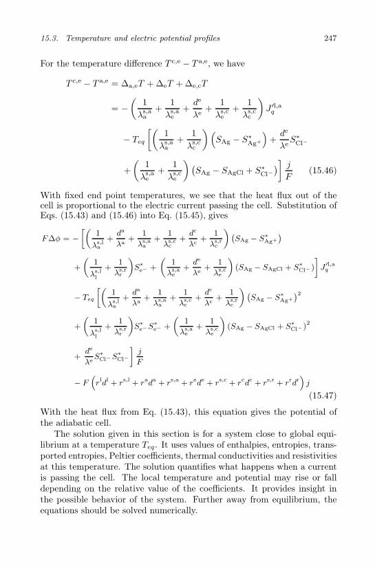
15.3. Temperature and electric potential profiles 247
For the temperature difference T c,e − T a,e, we have
T c,e − T a,e = ∆a,eT + ∆eT + ∆e,cT
= −(
1
λs,aa
+1
λs,ae
+de
λe+
1
λs,ce
+1
λs,cc
)J ′l,a
q
− Teq
[(1
λs,aa
+1
λs,cc
)(SAg − S∗
Ag+
)+de
λeS∗
Cl−
+
(1
λs,ae
+1
λs,ce
)(SAg − SAgCl + S∗
Cl−
)] jF
(15.46)
With fixed end point temperatures, we see that the heat flux out of thecell is proportional to the electric current passing the cell. Substitution ofEqs. (15.43) and (15.46) into Eq. (15.45), gives
F∆φ = −
»„
1
λs,la
+da
λa+
1
λs,aa
+1
λs,cc
+dc
λc+
1
λs,rc
«
`
SAg − S∗Ag+
´
+
„
1
λs,ll
+1
λs,rr
«
S∗e− +
„
1
λs,ae
+de
λe+
1
λs,ce
«
(SAg − SAgCl + S∗Cl−)
–
J ′l,aq
− Teq
»„
1
λs,la
+da
λa+
1
λs,aa
+1
λs,cc
+dc
λc+
1
λs,rc
«
`
SAg − S∗Ag+
´2
+
„
1
λs,ll
+1
λs,rr
«
S∗e−S
∗e− +
„
1
λs,ae
+1
λs,ce
«
(SAg − SAgCl + S∗Cl−)
2
+de
λeS∗
Cl−S∗Cl−
–
j
F
− F“
rldl + rs,l + rada + rs,a + rede + rs,c + rcdc + rs,r + rrdr”
j
(15.47)
With the heat flux from Eq. (15.43), this equation gives the potential ofthe adiabatic cell.
The solution given in this section is for a system close to global equi-librium at a temperature Teq. It uses values of enthalpies, entropies, trans-ported entropies, Peltier coefficients, thermal conductivities and resistivitiesat this temperature. The solution quantifies what happens when a currentis passing the cell. The local temperature and potential may rise or falldepending on the relative value of the coefficients. It provides insight inthe possible behavior of the system. Further away from equilibrium, theequations should be solved numerically.

This page intentionally left blankThis page intentionally left blank

Chapter 16
The Liquid Junction Potential
We describe a concentration cell with two aqueous electrolytes at constanttemperature. The magnitude and origin of the liquid junction potential isdetermined.
A precise description of liquid junctions in electrochemical cells is impor-tant in analytical chemistry [27,212–216]. Liquid junctions, or salt bridges,are used to separate electrolyte solutions. They are also used in referenceelectrodes. The exact relationship between the unknown concentration ofa species in a test solution and the cell potential is of interest. The testsolution contains the salt MX, and the cell has a X−-reversible electrodeand a reference electrode. Assume that two measurements are taken of thecell potential, ∆φ1 and ∆φ2. The Nernst equation has been used to linkthe concentrations of two test solutions, giving:
(∆φ1)j=0 − (∆φ2)j=0 =RT
FlncM+(1)
cM+(2)
(16.1)
In this chapter, we shall find the cell potentials ∆φ1 and ∆φ2 for a typicalcell, (16.2), so that we can test this relation. We shall calculate all thecontributions to the cell potential for a cell with a liquid junction andcompare the results with experimental values, see [214–216].
The most common reference electrode in analytical chemistry is theAg(s)| AgCl(s) electrode. It is often used in combination with a liquidjunction or a salt bridge. The concentration of salt, normally KCl, in thejunction is high, usually 4 kmol m−3. The salt KCl is used because themobilities of the cation and the anion are almost the same. The salt bridgeor the liquid junction is therefore assumed to give a negligible contributionto the cell potential. This contribution cancels when two potential valuesare subtracted, as in Eq. (16.1). We shall quantify this statement, using
249

250 Chapter 16. The Liquid Junction Potential
HCl in the test solution. Since the mobility of protons is higher than themobilities of other ions, a junction between HCl and KCl solutions is suitedfor an analysis of how and when the liquid junction contributes to the cellpotential. The experimental cell is thus
Ag(s)| AgCl(s)|HCl(aq, cHCl)||KCl(aq, cKCl)|AgCl(s)|Ag(s) (16.2)
The right hand side of the cell, |KCl(aq, cKCl)|AgCl(s)|Ag(s), is the refer-ence electrode mentioned above. To simplify matters, we have chosen theAg(s)|AgCl(s) electrode also on the left hand side. The solution compart-ments contain solutions of uniform composition of HCl and KCl, respec-tively. Inside the junction, denoted ||, the concentration of HCl decreasesfrom the value in the left reservoir, c(1)HCl, to zero in the right reservoir,c(2)HCl = 0, while the concentration of the KCl increases from zero in the left
reservoir, c(1)KCl = 0, to the value in the right reservoir, c(2)KCl. We considerthe situation when the cell compartments next to the junction have a largevolume compared to the junction, and are well stirred, so that all concen-tration gradients are located to the liquid junction. This is called restricteddiffusion. In practice, the liquid junction is a capillary with a porous plugthat prevents convection in the high density KCl solution.
The problem of the liquid junction is old, dating back to Planck [217,218]and Henderson [219,220]. Extensive discussions of liquid junctions and theiruse in salt bridges were given by Kotyk and Janacek [212] and Førlandet al. [27]. We shall derive the contribution to the potential differencefollowing the systematic procedure of the preceding sections, and updateearlier results [27] by more recent ones [215].
The cell temperature is constant. The disappearance of silver (silverchloride) on one side is therefore balanced by the appearance of silver (silverchloride) on the other side. The remaining salt contributions from theelectrode can be integrated with the electrolyte contribution to the totalcell potential, giving:
(∆φ)j=0 = (∆eφ)j=0 (16.3)
We shall find the cell potential by calculating the right hand side of thisequation. The agreement between calculated and experimental results ofthis type can be very good, within ±0.2 mV [215].
16.1 The flux equations for the electrolyte
Contributions to ∆φ arise from changes in chemical potentials. When theelectrode compartments are stirred, they have no chemical potential gradi-ents, and need not be considered. The liquid junction contributes by ∆eφ,

16.1. The flux equations for the electrolyte 251
the liquid junction potential. The liquid junction potential can be derivedfrom its entropy production. The entropy production in the junction hascontributions from the fluxes of both KCl and HCl as well as from theelectric current
σe = −JeKCl
1
T
∂
∂xµe
KCl − JeHCl
1
T
∂
∂xµe
HCl − j1
T
∂φe
∂x(16.4)
The frame of reference for the fluxes is water. The flux-force relations are,accordingly:
JeKCl = −Le
11
1
T
∂
∂xµe
KCl − Le12
1
T
∂
∂xµe
HCl − Le1φ
1
T
∂φe
∂x
JeHCl = −Le
12
1
T
∂
∂xµe
KCl − Le22
1
T
∂
∂xµe
HCl − Le2φ
1
T
∂φe
∂x
j = −Leφ1
1
T
∂
∂xµe
KCl − Leφ2
1
T
∂
∂xµe
HCl − Leφφ
1
T
∂φe
∂x
(16.5)
The transference coefficients are defined as
teKCl ≡ F
(Je
KCl
j
)
µKCl,µHCl
= FLe
1φ
Leφφ
teHCl ≡ F
(Je
HCl
j
)
µKCl,µHCl
= FLe
2φ
Leφφ
(16.6)
Using the Onsager’s relations, integration of Eq. (16.5c) together withEq. (16.6) gives the potential difference due to the liquid junction:
(∆eφ)j=0 =
∫ 2
1
dφe = − 1
F
∫ 2
1
(teKCldµeKCl + teHCldµ
eHCl) (16.7)
This is the formula for the liquid junction potential∗. For zero electriccurrent, the mass fluxes become
(JeKCl)j=0 = −le11
1
T
∂
∂xµe
KCl − le121
T
∂
∂xµe
HCl
(JeHCl)j=0 = −le12
1
T
∂
∂xµe
KCl − le221
T
∂
∂xµe
HCl
(16.8)
∗This definition of the liquid junction potential differs from what is normally used inthe literature, see e.g. [221], where only a part of ∆φ (namely ∆φ2, see below) is takenas due to the liquid junction.

252 Chapter 16. The Liquid Junction Potential
The diffusional coefficients leij are related to coefficients for mass and chargetransfer by
leij = Leij −
LeiφL
eφj
Leφφ
(16.9)
The concentration of the components KCl and HCl are everywhere de-fined by the concentration of their cations. The transference coefficients ofKCl and HCl are therefore identical to the transference numbers of K+ andH+, respectively. Following the analysis in Sec. 10.3, these can be expressedin terms of the mobilities, ue
K+ , ueH+ and ue
Cl−, and concentrations, ce
K+ , ceH+
and ceCl−
, of the ions. This results in, cf. Eq. (10.51),
teKCl = teK+ =
ueK+ceK+
ueK+ceK+ + ue
H+ceH+ + ueCl−
ceCl−
teHCl = teH+ =
ueH+ceH+
ueK+ceK+ + ue
H+ceH+ + ueCl−
ceCl−
(16.10)
The concentrations of the ions are related to the KCl and HCl concentra-tions by
ceK+ = ceKCl , ceH+ = ceHCl and ceCl− = ceKCl + ceHCl (16.11)
The electric conductivity of the solution is, cf. Eq. (10.36),
κe =Le
φφ
T=(ue
K+ceK+ + ueH+ceH+ + ue
Cl−ceCl−
)F (16.12)
For the other coefficients, we use Nernst–Einstein’s assumption, seeSec. 10.6,
Le12 = 0, Le
11 =Le
1φ
Fand Le
22 =Le
2φ
F(16.13)
By introducing these relations into the mass flux equations, we obtain theNernst–Planck flux equations
JeKCl = −κ
e
FteK+
∂
∂x(µe
KCl + Fφe)
JeHCl = −κ
e
FteH+
∂
∂x(µe
HCl + Fφe)
(16.14)
By introducing the electric potential gradient, using Eqs. (16.5c) and (16.6),we obtain
(JeKCl)j=0 = −κ
e
FteK+
[teH+
∂
∂x(µe
KCl − µeHCl) + te
Cl−∂
∂xµe
KCl
]
(JeHCl)j=0 = −κ
e
FteH+
[teK+
∂
∂x(µe
HCl − µeKCl) + te
Cl−∂∂xµ
eHCl
] (16.15)

16.2. The liquid junction potential 253
where we used teK+ + te
H+ + teCl−
= 1. The equations express that thereare two types of diffusion superimposed on each other, interdiffusion of twocations (the first term to the right), and diffusion of cation-anion pairs (thelast term to the right).
16.2 The liquid junction potential
The equations above determine the liquid junction potential. The chemicalpotentials are
µeKCl = µ0
KCl +RT ln aeKCl = µ0
KCl +RT ln(ceCl−
ceK+ye
KCl
)
µeHCl = µ0
HCl +RT ln aeHCl = µ0
HCl +RT ln(ceCl−
ceH+ye
HCl
) (16.16)
By introducing these chemical potentials and Eqs. (16.10) and (16.11) intoEq. (16.7), the liquid junction potential becomes:
(∆eφ)j=0
= − 1
F
∫ 2
1
(ue
K+ceK+dµeKCl + ue
H+ceH+dµeHCl
ueK+ceK+ + ue
H+ceH+ + ueCl−
ceCl−
)
= −RTF
∫ 2
1
[d ln ceCl− +
(ue
K+ − ueCl−
)dce
K+ +(ue
H+ − ueCl−
)dce
H+
ueK+ceK+ + ue
H+ceH+ + ueCl−
ceCl−
]
− RT
F
∫ 2
1
(ue
K+ceK+d ln yeKCl + ue
H+ceH+d ln yeHCl
ueK+ceK+ + ue
H+ceH+ + ueCl−
ceCl−
)(16.17)
In order to compare with expressions in the literature, we split the integralinto three terms:
(∆eφ)j=0 = ∆eφ1 + ∆eφ2 + ∆eφ3 (16.18)
The first term is due to a difference in salt concentration between thereservoirs at the ends of the junction:
∆eφ1 = −RTF
∫ 2
1
d ln ceCl− = −RTF
lnc(2)
Cl−
c(1)
Cl−
= −RTF
lnc(2)KCl
c(1)HCl
(16.19)
This contribution is the Nernst potential, see e.g. [221]. The contributionis zero when the concentrations are the same, c(2)KCl = c
(1)HCl (the Lewis–
Sargent cell). It leads to an expression of the type Eq. (16.1) when values

254 Chapter 16. The Liquid Junction Potential
for two HCl solutions are subtracted from one another. The remainingcontributions therefore give correction terms.
The second term is due to differences in the ionic mobilities
∆eφ2 = −RTF
∫ 2
1
(ue
H+ − ueCl−
)dce
H+
ueK+ceK+ + ue
H+ceH+ + ueCl−
ceCl−
− RT
F
∫ 2
1
(ue
K+ − ueCl−
)dce
K+
ueK+ceK+ + ue
H+ceH+ + ueCl−
ceCl−
(16.20)
The term is the leading term of the Lewis–Sargent cell. We see also thatKCl does not contribute much, as the mobilities of the K+ and the Cl−
ions are almost equal, see [97]. Equation (16.20) applies to a cell withtwo electrolytes. The name liquid junction potential has frequently beenassociated with this term alone.
The third contribution stems from variations in the activity coefficients
∆eφ3 = −RTF
∫ 2
1
(ue
K+ceK+d ln yeKCl + ue
H+ceH+d ln yeHCl
ueK+ceK+ + ue
H+ceH+ + ueCl−
ceCl−
)(16.21)
This contribution is frequently neglected. Values around 10 mV are typical(see the next section).
In order to integrate Eqs. (16.20) and (16.21), we must know the mobil-ities and activity coefficients as functions of the concentrations across thejunction. Equation (16.21) can only be integrated numerically. Hender-son [219, 220] had already integrated Eq. (16.20) in 1907, assuming linearprofiles for the concentrations. Take as the origin the start of the liquidjunction. Linear concentration profiles are given by
ceH+(x) = c
(1)HCl
dlj − x
dlj,
ceK+(x) = c
(2)KCl
x
dljand ce
Cl−(x) = c
(1)HCl
dlj − x
dlj+ c
(2)KCl
x
dlj
(16.22)
where dlj is the thickness of the liquid junction. By introducing theseconcentration profiles into Eq. (16.20), we obtain:
∆eφ2
=−
Z dlj
0
(RT/F )h
`
ueK+− ue
Cl−
´
c(2)KCl−
`
ueH+− ue
Cl−
´
c(1)HCl
i
d (x/dlj)
`
ueH+ + ue
Cl−
´
c(1)HCl+
h
`
ueK+ + ue
Cl−
´
c(2)KCl−
`
ueH+ + ue
Cl−
´
c(1)HCl
i
(x/dlj)
(16.23)

16.3. Liquid junction potential calculations compared 255
By integrating this expression, we have
∆eφ2 = −RTF
[(ue
K+ − ueCl−
)c(2)KCl −
(ue
H+ − ueCl−
)c(1)HCl(
ueK+ + ue
Cl−
)c(2)KCl −
(ue
H+ + ueCl−
)c(1)HCl
]
× ln
[(ue
K+ + ueCl−
)c(2)KCl(
ueH+ + ue
Cl−
)c(1)HCl
](16.24)
This is Henderson’s equation.
16.3 Liquid junction potential calculations compared
We shall compare calculated solutions of Eqs. (16.20) and (16.21) for threecases.
1. Concentration profiles from Eqs. (16.8) with diffusional coefficientsfrom Miller [72,73], and transference coefficients from Lindeberg [222].These calculations are the most precise ones. They predict the mea-sured potential across a known concentration gradient within ±0.2mV[215].
2. Concentration profiles from Eqs. (16.15), with assumption (16.13)for diffusion coefficients and accurate transference coefficients fromLindeberg [222].
3. Concentration profiles from Eqs. (16.15), with assumption (16.13) fordiffusion coefficients and transference coefficients from ionic mobilitiesat infinite electrolyte dilution (see Table 10.1).
The data was taken from various sources. Miller [73] estimated theconcentration dependence of diffusional mobilities in solutions of HCl andKCl from solutions with one electrolyte. The diffusional mobilities in hisLNI approximation, λij , are related to our coefficients by
lij =T∑3
k=1
∑3l=1 zkzl (λijλkl − λilλkj)∑3k=1
∑3l=1 zkλklzl
(16.25)
where zi is the ionic charge. The λij-coefficients are tabulated in Ref. [73].The ionic mobility, ui, for all ions i, has dimension ms−1/Vm−1 in the

256 Chapter 16. The Liquid Junction Potential
following formulae according to Lindeberg [222]:
FuH+ = 34.983− 11.7953√cH+/
(1 + 2.175
√cH+
)− 2.376cH+
− 3.856√cK+/
(1 + 0.468
√cK+
)+ 3.114cK+
FuK+ = 7.353 − 5.915√I/(1 + 2.501
√I)− 0.204I
FuCl− = 7.633 − 5.915√I/(1 + 2.501
√I)− 0.204I
(16.26)
where I is the (dimensionless) ionic strength of the solution, I = 12
∑ni ciz
2i .
The concentrations in the formulae have dimensions of kmol m−3, and Fis Faraday’s constant.
Activity coefficients for the electrolytes in their mixtures were takenfrom MacInnes [223]. A quadratic term in cKCl was added to fit newerexperimental data [224].
ln yHCl = −2.3284√I/[1 + 1.30
√I]
+ 0.4472cHCl + 0.3050cKCl + 0.03c2KCl
ln yKCl = −2.3444√I/[1 + 1.294
√I]
+ 0.04738I + 0.01985I2
(16.27)
The three calculated concentration profiles are shown in Fig. 16.1 for ajunction of unit thickness (i.e. the actual thickness was used as the unit).The stippled lines were calculated for case 1 above, while the solid linesrepresent cases 2 and 3 (inseparable). A linear variation in concentrationis also shown.
The concentrations of KCl and HCl in this figure were cKCl(2) = 4kmol m−3 and cHCl(1) = 0.1 kmol m−3, respectively. All profiles showthat the concentration of HCl in the junction is always smaller than thatgiven by a linear variation. The situation for KCl depends on the methodof calculation. However, the deviation from a linear profile is smaller than10%. We explain the deficit of HCl in the junction compared to that givenby a linear profile by the high mobility of H+.
The next step was to calculate the cell potential for the different con-centration profiles. Cases 2 and 3, naturally, did not give results that weresignificantly different from one another. Cases 1 and 2 deviated in theirprediction of the measured stationary state cell potential by ±1 mV. Whenthese results were compared to a potential integrated for linear concentra-tion profiles (Henderson’s approximation, see Eq. (16.24)), ∆φ2 and ∆φ3
were underestimated by 0.1 mV. We conclude that even if the concentra-tion profiles seem different, they do not have an important impact on the

16.3. Liquid junction potential calculations compared 257
Figure 16.1 The three calculated concentration profiles for a junction of unitthickness. The dashed lines were calculated for case 1 above, while the solidlines represent cases 2 and 3 (inseparable). A linear variation in concentrationis also shown. Reproduced from Zeitschr. Phys. Chemie 174 (1991) 179–198with permission from Oldenburg Wissenschaftsverlag [215].
cell potential. An explanation may be that the sequence of thermodynamicstates that make up the path of integration is more important than its ac-tual location in space. The difference between the states that are traversedin Cases 1 and 2 is small.
All contributions to the cell potential vary with the concentrations inthe reservoirs, see Table 16.1 and Figs. 16.1 and 16.2. The table shows thecalculated contributions to the measured cell potential for selected reservoirconcentrations of Case 2. The figures give further information on ∆φ2 and∆φ3, respectively.
The term ∆φ1 gives the major contribution to the cell potential. WhencKCl = 4 kmol m−3 and cHCl decrease from 0.1 to 0.001 kmol m−3, this termvaried from 95 to 213 mV. The Nernst term predicted the total potentialwithin 10% for the concentration combinations given in Table 16.1. If abetter accuracy is needed in the analysis, the other terms must be takeninto account.

258 Chapter 16. The Liquid Junction Potential
Table 16.1 Contributions to the liquid junction potential at 298 K in cell d,Ag(s)|AgCl(s)|HCl(aq, cKCl)‖KCl(aq, cHCl)| AgCl(s)|Ag(s). The contributionsare calculated with Nernst–Einstein’s assumption (16.13)
cHCl ∆φ1 ∆φ2 ∆φ3 Total cell cKCl
Nernst- Mobility- Activity- potential/kmol m−3 term / mV term / mV term / mV /mV /kmol m−3
0.1 94.8 −4.3 −2.6 88.0 40.01 153.9 −3.6 −8.6 141.8 –0.001 213.1 −4.5 −10.0 198.7 –
0.1 41.4 −14.8 −4.5 22.2 0.50.01 100.5 −4.8 −9.2 86.6 –0.001 159.7 −3.3 −10.4 146.0 –
The variation in ∆φ2 gives the main deviation between the Nernst equa-tion and the total cell potential in most cases (see Table 16.1). The termis the most important at low concentrations of the two electrolytes. Inasymmetrical cells like the ones given in the table, the contribution is ofthe order of 5 mV. The term can to good approximation be determined us-ing constant ionic mobilities in Eqs. (16.20) and (16.21): The contributionfrom mobility differences changed less than 1 mV by replacing the concen-tration dependent mobilities with mobilities at infinitely dilution, see Breeret al. [215].
The variation in ∆φ3 (see Fig. 16.2) increases in importance from 2 to10% as cHCl decreases from 0.1 to 0.001 kmol m−3. The variation seems toapproach an upper limit as cHCl → 0 (see the upper curve in Fig. 16.2).This term can be neglected when HCl and KCl are both dilute. The liquidjunction potential, as defined here, included the Nernst contribution, ∆φ1.The Nernst contribution alone most often does not give sufficient accuracyin concentration determinations. An accurate method for the calculationof the correction term is then needed.
16.4 Concluding comments
We have seen, i.e. from Table 16.1, that the Nernst equation (16.1) is notsufficient for accurate calculations of solution concentrations of ions frommeasurements of cell potentials in cells with liquid junctions. The cellpotential of isothermal concentration cells can, however, be obtained withreasonable accuracy by integrating across the liquid junction using constantionic mobilities, and by using Nernst–Einstein’s or Henderson’s assumptionsto find the concentration gradients.

16.4. Concluding comments 259
Figure 16.2 The contribution to the cell potential from the activity coef-ficient, here called E2 (corresponding to ∆φ3 in the text), as a functionof KCl concentration for different HCl concentrations. Reproduced fromZeitschr. Phys. Chemie 174 (1991) 179–198 with permission from OldenburgWissenschaftsverlag [215].
In order to increase the accuracy of the calculation further, activity co-efficients must be used. Such information is frequently not known. Thisgives one the motivation for efforts to find a replacement of the liquid junc-tion. A solid state reference electrode [225] does not have the disadvantagesof the calomel electrode.
We have shown how the theoretical method is well suited for the evalu-ation of experimental results. The possibility to test assumptions that aremade in the theory is important for further developments.

This page intentionally left blankThis page intentionally left blank

Chapter 17
The Formation Cell
We describe conversion of chemical energy into electrical energy in forma-tion cells. We find the electric potential profile across the cell from thecorresponding variations in chemical potential and/or temperature at zeroelectric current density.
Electrochemical energy conversion was the main topic of Chapters 13–16. It will be continued here for the most important electrochemical cell,the formation cell. Such cells have different electrodes. Common ex-amples are batteries, fuel cells and electrolysis cells. The literature onthese systems is enormous. The aim of this chapter is to see how non-equilibrium thermodynamics can be used to describe the profiles in inten-sive variables of a formation cell taking advantage of the lessons learned inChapters 13–16.
A systematic description of the coupled transports of heat, mass andcharge in formation cells is obtained from the entropy production of thevarious phases of the cell [129, 226]. Only the electrolyte phase was stud-ied earlier [189, 227, 228]. The flux equations relate thermoelectric effects,concentration cell effects and the chemical reactions in the formation cell.Thermoelectric effects and concentration cells were described in Chapters13–16. The position dependent transference coefficient and the position de-pendent Peltier coefficient (see Chapter 13) are needed here in order tointegrate across the cell.
In order to take advantage of the results in Chapters 13 and 15, we usethe electrodes that were described in these chapters. The formation cellexample becomes:
Fe(s)|Na(Hg)|NaCl(aq)|AgCl(s)|Ag(s) (17.1)
The cell has an amalgam electrode to the left, and is connected to thepotentiometer by an iron lead. The amalgam electrode on the left hand side
261

262 Chapter 17. The Formation Cell
was described in Sec. 13.1. The right hand side electrode, is the Ag|AgClelectrode, which was described in Secs. 15.1–3. The silver is connected tothe other side of the potentiometer directly. The left hand side electrodereaction is:
Na (Hg) → Na+(aq) + e− (17.2)
One mole of Na disappears from the amalgam into the electrolyte per moleof electrons passing the external circuit from left to right. At the surfaceof the chloride layer that faces the electrolyte we have:
AgCl (s) → Cl−(aq) + Ag+ (17.3)
One mole of Cl− is produced in the electrolyte, while one mole of silverions is produced in the chloride, close to this surface. The silver ions aretransported to the surface between the chloride layer and the metal. Theright hand side electrode reaction
Ag+ + e− → Ag(s) (17.4)
takes place at the surface between the metal and the chloride. The totalcell reaction is:
Na(Hg) + AgCl(s) → Na+(aq) + Cl−(aq) + Ag(s) (17.5)
One mole of Ag(s) and of NaCl(aq) are produced and one mole of Na(Hg)and AgCl(s) are consumed per faraday passing the cell.
In the electrolyte the total amount of dissolved NaCl goes up with onemole per faraday passing the cell. Because of the electroneutral natureof the electrolyte, the concentrations of the sodium and the chloride ionsare the same at every position in the electrolyte. When the sodium ionenters the electrolyte from the amalgam surface, it is therefore quicklyaccompanied by a chloride ion coming into the electrolyte from the AgClsurface. The integrated divergence of the NaCl flux is equal to one moleper faraday passing the cell.
The method of analysis uses, just as in Chapters 13–16, neutral com-ponents as thermodynamic variables. Since the use of ionic componentsis more common, we shall also show how the transition between these for-mulations can be made. We shall refer extensively to Chapters 13–16 andapply formulae that were derived for the electrodes in these chapters. Inthis manner, the present chapter can focus on the boundary conditionsthat are special for the formation cell. We use the terminology given inChapters 9 and 13, see Figs. 9.1 and 13.2. The isothermal cell is consideredfirst as a reference, before we deal with the non-isothermal cell.
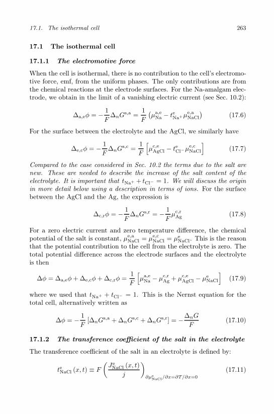
17.1. The isothermal cell 263
17.1 The isothermal cell
17.1.1 The electromotive force
When the cell is isothermal, there is no contribution to the cell’s electromo-tive force, emf, from the uniform phases. The only contributions are fromthe chemical reactions at the electrode surfaces. For the Na-amalgam elec-trode, we obtain in the limit of a vanishing electric current (see Sec. 10.2):
∆a,eφ = − 1
F∆nG
s,a =1
F
(µa,e
Na − teNa+µe,aNaCl
)(17.6)
For the surface between the electrolyte and the AgCl, we similarly have
∆e,cφ = − 1
F∆nG
s,c =1
F
[µc,e
AgCl − teCl−µe,cNaCl
](17.7)
Compared to the case considered in Sec. 10.2 the terms due to the salt arenew. These are needed to describe the increase of the salt content of theelectrolyte. It is important that tNa+ + tCl− = 1. We will discuss the originin more detail below using a description in terms of ions. For the surfacebetween the AgCl and the Ag, the expression is
∆c,rφ = − 1
F∆nG
s,r = − 1
Fµc,r
Ag (17.8)
For a zero electric current and zero temperature difference, the chemicalpotential of the salt is constant, µe,a
NaCl = µe,cNaCl = µe
NaCl. This is the reasonthat the potential contribution to the cell from the electrolyte is zero. Thetotal potential difference across the electrode surfaces and the electrolyteis then
∆φ = ∆a,eφ+ ∆e,cφ+ ∆c,rφ =1
F
[µa,e
Na − µc,rAg + µc,e
AgCl − µeNaCl
](17.9)
where we used that tNa+ + tCl− = 1. This is the Nernst equation for thetotal cell, alternatively written as
∆φ = − 1
F[∆nG
s,a + ∆nGs,c + ∆nG
s,r] = −∆nG
F(17.10)
17.1.2 The transference coefficient of the salt in the electrolyte
The transference coefficient of the salt in an electrolyte is defined by:
teNaCl (x, t) ≡ F
(Je
NaCl (x, t)
j
)
∂µeNaCl
/∂x=∂T/∂x=0
(17.11)

264 Chapter 17. The Formation Cell
Depending on the boundary conditions, the transference coefficient may beposition-, and possibly also time-dependent. When the chemical potentialand the temperature are constant, the salt concentration is independent ofthe position in the electrolyte, ceNaCl (t). The time-dependence of the saltconcentration satisfies
∂
∂tceNaCl (t) = − ∂
∂xJe
NaCl (x, t) (17.12)
where JeNaCl is the salt flux. By integrating this equation from x = 0 to
x = de, we obtain
∂
∂t
∫ de
0
ceNaCl (t) dx = −JeNaCl (de, t) + Je
NaCl (0, t) = Je,aNaCl (t) − Je,c
NaCl (t)
(17.13)The accumulation of salt in the electrolyte per unit of cross-sectional areais the difference in the salt flux at the two electrodes. The integrated saltcontent in the electrolyte increases with j/F moles of NaCl per unit of timeand per unit of cross sectional area. The increase in the salt content in theelectrolyte is therefore given by:
∂
∂tceNaCl (t) =
j
deF(17.14)
Equation (17.13) together with Eq. (17.14) imply that the salt flux is in-dependent of time. For the gradient of the transference coefficient, wetherefore find
∂
∂xteNaCl (x, t) =
F
j
∂
∂xJe
NaCl (x, t) = −Fj
∂
∂tceNaCl (t) = − 1
de(17.15)
It follows that the transference coefficient is independent of time and givenby
teNaCl (x) = teNa+ − x
de= teNa+
(1 − x
de
)− teCl−
x
de(17.16)
The integration constant has been chosen such that the average of thetransference coefficient over the electrolyte is equal to 0.5
(teNa+ − te
Cl−
).
An alternative derivation of the potential difference across the electrolyte,using a description in terms ionic fluxes and forces (see below), shows thatthis is the correct choice of the integration constant.
The transference coefficient of the salt is equal to the transference num-ber of the sodium ion, te
Na+ , at the anode surface and equal to minus thetransference number of the chloride ion, −te
Cl−= −(1− te
Na+), at the cath-ode surface (the interface between the electrolyte and AgCl). The ionictransfer numbers are weak functions of concentrations and will be takenconstant.

17.1. The isothermal cell 265
Remark 17.1. The relation between the ion fluxes, the salt flux and theelectric current depends on the electrode surface reactions. As a consequencethe transference coefficient of a salt also depends on the electrode surfacereactions [227]. In the formation cell, where the electrodes are different,this leads to position dependent transference coefficients for salts.
17.1.3 An electrolyte with a salt concentration gradient
The electrolyte has one independent component, the salt NaCl. The en-tropy production is
σe = −JeNaCl
1
T
∂
∂xµe
NaCl − j1
T
∂φ
∂x(17.17)
The frame of reference for the salt flux is water. The flux equations are
JeNaCl = −Le
µµ
1
T
∂
∂xµe
NaCl − Leµφ
1
T
∂φ
∂x
j = −Leφµ
1
T
∂
∂xµe
NaCl − Leφφ
1
T
∂φ
∂x
(17.18)
The transference coefficient was defined in Eq. (17.11) and satisfies:
teNaCl (x) ≡ F
(Je
NaCl (x)
j
)
∂µeNaCl
/∂x=∂T/∂x=0
= FLe
µφ
Leφφ
(17.19)
In the limit of a vanishing electric current, we find, using Onsager relations,the reversible contribution to the potential gradient
(∂φ
∂x
)
j→0
= − teNaCl
F
∂
∂xµe
NaCl (17.20)
The corresponding potential difference is thus
∆eφ =
∫ e,c
e,a
dφ = −∫ e,c
e,a
teNaCl
Fdµe
NaCl (17.21)
We now assume that the variation of the chemical potential across theelectrolyte is linear in x. Furthermore, using Eq. (17.16) this results in
∆eφ = − 1
2F
(teNa+ − teCl−
)(µe,c
NaCl − µe,aNaCl) = − 1
2F
(teNa+ − teCl−
)∆eµ
eNaCl
(17.22)

266 Chapter 17. The Formation Cell
For dilute solutions, we can use the ideal expression for the chemical po-tentials and obtain:
∆eφ = −RTF
(teNa+ − teCl−
)ln
(ce,cNaCl
ce,aNaCl
)= −RT
F
ueNa+ − ue
Cl−
ueNa+ + ue
Cl−
ln
(ce,cNaCl
ce,aNaCl
)
(17.23)
We derived the formula using neutral components and fluxes. The ionictransference numbers were expressed in terms of mobilities in the finalequality using Eq. (10.51), which gives:
teNa+ =ue
Na+
ueNa+ + ue
Cl−and teCl− =
ueCl−
ueNa+ + ue
Cl−(17.24)
The same expression was obtained already by Planck [217, 218] using theelectroneutrality condition JNa+ = JCl− and Nernst–Planck flux equations.It is called the Planck potential. The transference number of Na+ is 0.396,while the transference number of Cl− is 0.604, both at infinite dilution ofthe electrolyte in water. With a tenfold change in concentration across thecell, the electrolyte contribution becomes 11.8 mV. This value is normallynegligible compared to the contribution from the electrodes. It is required,however, in order to find the potential profile across the cell.
The effect of the different boundary conditions in a cell with two iden-tical electrodes and the formation cell can now be compared. When bothelectrodes are reversible to the Na+-ion, the corresponding expression was
∆eφ =2RT
FteCl− ln
(ce,cNaCl
ce,aNaCl
)(17.25)
This expression can be obtained from Eq. (10.56) for j = 0 by replac-ing AgNO3 by NaCl. The magnitude of the contribution is in both casessome mV.
The total potential difference across electrode surfaces and electrolyteis, finally,
∆φ = ∆a,eφ+ ∆eφ+ ∆e,cφ+ ∆c,rφ
=1
F
[µa,e
Na − µc,rAg + µc,e
AgCl − tNa+µe,aNaCl − tCl−µ
e,cNaCl
− 1
2
(teNa+ − teCl−
)∆eµ
eNaCl
]
=1
F
[µa,e
Na − µc,rAg + µc,e
AgCl −1
2(µe,a
NaCl + µe,cNaCl)
](17.26)

17.1. The isothermal cell 267
where we used Eq. (17.6) for ∆a,eφ, Eq. (17.7) for ∆e,cφ and Eq. (17.8) for∆c,rφ. For a constant concentration of the salt, the above expression reducesto the one, Eq. (17.9), given in the previous subsection. The differencebetween Eq. (17.26) and Eq. (17.9) is that Eq. (17.26) contains the averagechemical potential of the salt.
17.1.4 The Planck potential derived from ionic fluxes and forces
Planck [217,218] derived the expression for his potential from a descriptionthat uses ions as components. In the ionic formulation (see Sec. 10.6) onewrites the entropy production in the electrolyte as:
σe = JeNa+
[− 1
T
∂
∂x
(µe
Na+ + Fψe)]
+ JeCl−
[− 1
T
∂
∂x
(µe
Cl− − Fψe)]
(17.27)where ψe is the electrostatic potential (Maxwell potential), and the combi-nations of the chemical and the electrostatic potentials are the electrochem-ical potentials. Because the anode surface reaction is reversible to Na+ andnot to Cl−, while the cathode surface reaction is reversible to Cl− and notto Na+, the relations between the fluxes is:
JeNa+ =
j
2F+ Je
NaCl and JeCl− = − j
2F+ Je
NaCl (17.28)
or equivalently,
j
F= Je
Na+ − JeCl− and Je
NaCl =1
2
(Je
Na+ + JeCl−
)(17.29)
Eliminating the ionic fluxes from Eq. (17.27) using Eq. (17.28), the entropyproduction becomes
σe = −JeNaCl
1
T
∂
∂xµe
NaCl − j1
T
∂
∂x
(ψ +
µeNa+
2F−µe
Cl−
2F
)(17.30)
Comparing this relation with Eq. (17.17), we identify
φ = ψ +µe
Na+
2F−µe
Cl−
2F(17.31)
The linear flux-force relations that follow from the entropy productiongiven in Eq. (17.27) are:
JeNa+ = −L++ 1
T
∂
∂x
(µe
Na+ + Fψ)− L+− 1
T
∂
∂x
(µe
Cl−− Fψ
)
JeCl−
= −L−+ 1
T
∂
∂x
(µe
Na+ + Fψ)− L−− 1
T
∂
∂x
(µe
Cl−− Fψ
)(17.32)
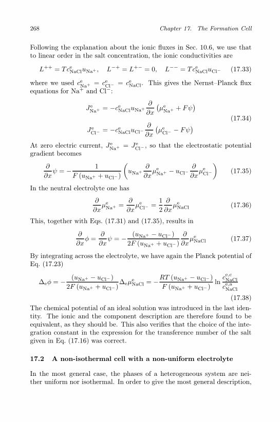
268 Chapter 17. The Formation Cell
Following the explanation about the ionic fluxes in Sec. 10.6, we use thatto linear order in the salt concentration, the ionic conductivities are
L++ = TceNaCluNa+ , L−+ = L+− = 0, L−− = TceNaCluCl− (17.33)
where we used ceNa+ = ce
Cl−= ceNaCl. This gives the Nernst–Planck flux
equations for Na+ and Cl−:
JeNa+ = −ceNaCluNa+
∂
∂x
(µe
Na+ + Fψ)
JeCl−
= −ceNaCluCl−∂
∂x
(µe
Cl−− Fψ
)(17.34)
At zero electric current, JeNa+ = Je
Cl−, so that the electrostatic potential
gradient becomes
∂
∂xψ = − 1
F (uNa+ + uCl−)
(uNa+
∂
∂xµe
Na+ − uCl−∂
∂xµe
Cl−
)(17.35)
In the neutral electrolyte one has
∂
∂xµe
Na+ =∂
∂xµe
Cl− =1
2
∂
∂xµe
NaCl (17.36)
This, together with Eqs. (17.31) and (17.35), results in
∂
∂xφ =
∂
∂xψ = − (uNa+ − uCl−)
2F (uNa+ + uCl−)
∂
∂xµe
NaCl (17.37)
By integrating across the electrolyte, we have again the Planck potential ofEq. (17.23)
∆eφ = − (uNa+ − uCl−)
2F (uNa+ + uCl−)∆eµ
eNaCl = −RT (uNa+ − uCl−)
F (uNa+ + uCl−)lnce,cNaCl
ce,aNaCl
(17.38)
The chemical potential of an ideal solution was introduced in the last iden-tity. The ionic and the component description are therefore found to beequivalent, as they should be. This also verifies that the choice of the inte-gration constant in the expression for the transference number of the saltgiven in Eq. (17.16) was correct.
17.2 A non-isothermal cell with a non-uniform electrolyte
In the most general case, the phases of a heterogeneous system are nei-ther uniform nor isothermal. In order to give the most general description,

17.2. A non-isothermal cell with a non-uniform electrolyte 269
we shall need to refer a property under evaluation to a temperature. Forinstance, the chemical potential at the surface, µs,a
Na, is normally, but notalways, evaluated at the surface temperature, T s,a. If the quantity is eval-uated at a different temperature this will be explicitly indicated. Thus thechemical potential of the sodium in the bulk anode close to the surface,µa,e
Na(Ts,a), is evaluated at the temperature of the surface. Again we limit
ourselves to stationary states, defined here as states for which all fluxesare independent of the time. When integrating across the homogeneousregions, we neglect as before the temperature variation of entropies andtransported entropies in order to be able to give an analytical result. Theseresults can be extended using numerical integration.
17.2.1 The homogeneous anode phase
The entropy production in the amalgam electrode is given by
σa = −J ′aq
1
T 2
∂T
∂x− Ja
Na
1
T
∂
∂xµa
Na,T − j1
T
∂φ
∂x(17.39)
The resulting linear flux-force relations are
J ′aq = −La
1
T 2
∂T
∂x− La
qµ
1
T
∂
∂xµa
Na,T − Laqφ
1
T
∂φ
∂x
JaNa = −La
µq
1
T 2
∂T
∂x− La
µµ
1
T
∂
∂xµa
Na,T − Laµφ
1
T
∂φ
∂x
j = −Laφq
1
T 2
∂T
∂x− La
φµ
1
T
∂
∂xµa
Na,T − Laφφ
1
T
∂φ
∂x
(17.40)
The position dependent transference coefficient for NaCl was discussed inSec. 17.1 (see Eq. (17.16)). In the present case, the flux of sodium is zeroin x = −da and equal to j/F in x = 0. The transference coefficient in thiscase is given by
taNa (x) ≡ F
(Ja
Na(x)
j
)
∂T/∂x=∂µaNa
/∂x=0
= FLa
µφ(x)
Laφφ
= 1 +x
da(17.41)
The position dependent Peltier coefficient is defined analogously, from ananalysis of the divergence of the heat flux and the resulting heat production:
πa(x) ≡ F
(J ′a
q (x)
j
)
∂T/∂x=∂µaNa
/∂x=0
= FLa
qφ(x)
Laφφ
= −T (x)[taNa(x)S
aNa + S∗,a
e−
](17.42)

270 Chapter 17. The Formation Cell
The position dependent Peltier coefficient is given by the entropy of Naand the transported entropy of the electrons. The derivation is analogousto the one in the electrolyte. Note that πa,0 = πa(−da) and πa,e = πa(0).
Using Onsager’s relations and the definitions of the transference num-ber of Na and the Peltier coefficient, we find for the zero current electricpotential gradient:
(∂φ
∂x
)
j→0
= − 1
F
[taNa(x)
∂
∂xµa
Na,T +πa(x)
T (x)
∂T
∂x
]
= − 1
F
[taNa(x)
(∂
∂xµa
Na + SaNa
∂T
∂x
)+πa(x)
T (x)
∂T
∂x
]
= − 1
F
[(1 +
x
da
)∂
∂xµa
Na − S∗,ae−∂T
∂x
](17.43)
By integrating across the electrode, taking the chemical potential andthe temperature profiles linear, we obtain for the zero current potentialdifference:
∆aφ = − 1
2F∆aµ
aNa +
1
FS∗,a
e−∆aT (17.44)
where we note that ∆aµaNa = µa,e
Na (T a,e) − µa,oNa (T a,o). Using the ideal
expression for the chemical potential gives
∆aφ = −RT2F
lnca,eNa
ca,oNa
+1
FS∗,a
e−∆aT (17.45)
Under conditions when ca,oNa > ca,eNa, the first contribution will be positive.For stirred amalgam ∆aµ
aNa = 0, in which case this term does not con-
tribute. When we add the first term in Eq. (17.44) to Eq. (17.9), and inEq. (17.26), the contribution µa,e
Na changes to the average 0.5(µa,eNa +µa,o
Na) inboth equations.
17.2.2 The electrolyte
By including the contribution due to the temperature gradient inEq. (17.17), the entropy production in the electrolyte is given by
σe = −J ′eq
1
T 2
∂T
∂x− Je
NaCl
1
T
∂
∂xµe
NaCl,T − j1
T
∂φ
∂x(17.46)

17.2. A non-isothermal cell with a non-uniform electrolyte 271
The resulting linear flux-force relations are
J ′eq = −Le
1
T 2
∂T
∂x− Le
qµ
1
T
∂
∂xµe
NaCl,T − Leqφ
1
T
∂φ
∂x
JeNaCl = −Le
µq
1
T 2
∂T
∂x− Le
µµ
1
T
∂
∂xµe
NaCl,T − Leµφ
1
T
∂φ
∂x
j = −Leφq
1
T 2
∂T
∂x− Le
φµ
1
T
∂
∂xµe
NaCl,T − Leφφ
1
T
∂φ
∂x
(17.47)
The position dependent transference coefficient, teNaCl(x), was discussed inSec. 17.1, see Eq. (17.16). The position dependent Peltier coefficient isdefined analogously, from an analysis of the divergence of the heat flux andthe resulting heat production:
πe(x) ≡ F
(J ′e
q (x)
j
)
∂T/∂x=∂µeNaCl
/∂x=0
= FLe
qφ(x)
Leφφ
= T (x)
[−teNaCl(x)S
eNaCl +
(1 − x
de
)teNa+S
∗,eNa+ − x
deteCl−S
∗,eCl−
]
(17.48)
The position dependent Peltier coefficient is given by the entropy of NaCland transported entropies of its ions. The transported entropies enter theanalysis as integration constants at the surfaces, just as the transferencenumbers did in the expression for the transference coefficient. Note thatπe,a = πe(0) and πe,c = πe(de).
Using Onsager’s relations and the definitions of the transference numberof NaCl and the Peltier coefficient in Eq. (17.47c), we find for the currentlesselectric potential gradient:
(∂φ
∂x
)
j→0
= − 1
F
[teNaCl(x)
∂
∂xµe
NaCl,T +πe(x)
T (x)
∂T
∂x
]
= − 1
F
[teNaCl(x)
(∂
∂xµe
NaCl + SeNaCl
∂T
∂x
)+πe(x)
T (x)
∂T
∂x
]
= − 1
F
[(teNa+ − x
de
)∂
∂xµe
NaCl +
((1 − x
de
)teNa+S
∗,eNa+
− x
deteCl−S
∗,eCl−
)∂T
∂x
](17.49)

272 Chapter 17. The Formation Cell
By integrating across the electrolyte, taking the chemical potential and thetemperature profiles to be linear, we obtain for the zero current potentialdifference:
∆eφ = − 1
2F
(teNa+ − teCl−
)∆eµ
eNaCl −
1
2F
(teNa+S
∗,eNa+ − teCl−S
∗,eCl−
)∆eT
(17.50)
where we note that ∆eµeNaCl = µe,c
NaCl (Te,c)−µe,a
NaCl (Te,a). We have assumed
that the transported entropies were constant in the integration. The firstcontribution is probably larger than the second. We did not introduce aSoret equilibrium in the electrolyte.
17.2.3 The surface of the anode
The electrode reaction at the interface between Na(Hg) and NaCl(aq) isgiven in Eq. (17.2). The contribution to the reaction Gibbs energy due tothe neutral components is, cf. Eq. (17.6):
∆nGs,a = −µa,e
Na(Ts,a) + teNa+µ
e,aNaCl(T
s,a) (17.51)
for the non-isothermal case. The entropy production in the non-isothermalanode surface is:
σs,a = J ′a,eq
(1
T s,a− 1
T a,e
)+ J ′e,a
q
(1
T e,a− 1
T s,a
)− rs,a
∆nGs,a
T s,a− j
∆a,eφ
T s,a
(17.52)
The reaction rate is given in terms of the electric current, rs,a = j/F. Thisresults in
σs,a = J ′a,eq ∆a,s
(1
T
)+J ′e,a
q ∆s,e
(1
T
)− j
1
T s,a
[∆a,eφ+
∆nGs,a
F
](17.53)
The flux equations are accordingly
J ′a,eq = Ls,a
aa∆a,s
(1
T
)+ Ls,a
ae ∆s,e
(1
T
)− Ls,a
aφ
1
T s,a
[∆a,eφ+
∆nGs,a
F
]
J ′e,aq = Ls,a
ea ∆a,s
(1
T
)+ Ls,a
ee ∆s,e
(1
T
)− Ls,a
eφ
1
T s,a
[∆a,eφ+
∆nGs,a
F
]
j = Ls,aφa∆a,s
(1
T
)+ Ls,a
φe∆s,e
(1
T
)− Ls,a
φφ
1
T s,a
[∆a,eφ+
∆nGs,a
F
]
(17.54)

17.2. A non-isothermal cell with a non-uniform electrolyte 273
The Peltier coefficients for the bulk phases at the anode surface are:
πa,e ≡ F
„
J ′a,eq
j
«
∆a,sT=∆s,eT=∆s,eµNaCl=0
= FLs,a
aφ
Ls,aφφ
= −T a,e`
Sa,eNa + S∗,a,e
e−
´
πe,a ≡ F
„
J ′e,aq
j
«
∆a,sT=∆s,eT=∆s,eµNaCl=0
= FLs,a
eφ
Ls,aφφ
= T e,ateNa+
`
S∗,e,a
Na+ − Se,aNaCl
´
(17.55)
We see that πa,e = πa(0) and πe,a = πe(0), cf. Eqs. (17.42) and (17.48).The Peltier coefficient can be regarded as a transference coefficient of heat.It depends on the location in the same manner.
By using Onsager’s relations, the potential difference across the anodesurface becomes
∆a,eφ = −1
F
»
∆nGs,a + πa,e
„
T s,a − T a,e
T a,e
«
+ πe,a
„
T e,a − T s,a
T e,a
«–
= −1
F
ˆ
−µa,eNa + teNa+µ
e,aNaCl − S∗,a,e
e−(T s,a − T a,e) + teNa+S
∗,e,a
Na+ (T e,a − T s,a)˜
(17.56)
The main contribution to the surface potential drop is given by the reactionGibbs energy. For constant temperature at the surface, this expressionreduces to the one given in Eq. (17.6).
17.2.4 The homogeneous phases and the surface of the cathode
The chemical reaction that produces Cl− in the electrolyte and Ag+ toconduct charge in AgCl is given by Eq. (17.3). The contribution to thereaction Gibbs energy due to the neutral components is:
∆nGs,c = teCl−µ
e,cNaCl (T
s,c) − µc,eAgCl (T
s,c) (17.57)
The entropy production of the electrolyte-AgCl surface is:
σs,c = J ′e,cq ∆e,s
(1
T
)+J ′c,e
q ∆s,c
(1
T
)−j 1
T s,c
[∆c,eφ+
1
F∆nG
s,c
](17.58)
The Peltier coefficients are then
πe,c ≡ F
„
J ′e,cq
j
«
∆e,sT=∆s,cT=∆e,sµeNaCl
=0
= FLs,c
eφ
Ls,cφφ
= T e,cteCl−
`
Se,cNaCl − S∗,e,c
Cl−
´
πc,e ≡ F
„
J ′c,eq
j
«
∆e,sT=∆s,cT=∆e,sµeNaCl
=0
= FLs,c
cφ
Ls,cφφ
= T c,e“
S∗,c,e
Ag+ + Sc,eAgCl
”
(17.59)

274 Chapter 17. The Formation Cell
The zero current potential difference is accordingly:
∆e,cφ = − 1
F
[∆nG
s,c +πe,c
T e,c∆e,sT +
πc,e
T c,e∆s,cT
]
= − 1
F
[teCl−µ
e,cNaCl − µc,e
AgCl − teCl−S∗,eCl−
∆e,sT + S∗,cAg+∆s,cT
](17.60)
Entropies and transported entropies were taken constant in the integration,as usual.
The electric potential drop across the bulk phase of AgCl is given byEq. (15.14) for zero current:
∆cφ = − 1
FS∗,c
Ag+∆cT (17.61)
The electrochemical reaction taking place between the pure phases of silverand silver chloride is given by Eq. (17.4). The contribution to the reactionGibbs energy ∆nG
s,r due to the neutral components is:
∆nGs,r = µr,c
Ag (T s,r) (17.62)
Analogous to the derivation of Eq. (17.60), we obtain, for the currentlesspotential difference
∆c,rφ = − 1
F
[∆nG
s,r +πc,r
T c,r∆c,sT +
πr,c
T r,c∆s,rT
]
= − 1
F
[µr,c
Ag + S∗,cAg+∆c,sT − S∗,r
e−∆s,rT
](17.63)
where the Peltier coefficients are given by
πc,r = T c,rS∗,cAg+ and πr,c = −T r,c
(Sr
Ag + S∗,re−
)(17.64)
The potential difference across the silver cathode for j = 0 is:
∆rφ =
∫ r.o
r,c
dφ =1
FS∗,r
e ∆rT (17.65)

17.3. Concluding comments 275
17.2.5 The cell potential
By adding all contributions to the cell potential, we have the electromotiveforce:
∆φ = ∆aφ+ ∆a,eφ+ ∆eφ+ ∆e,cφ+ ∆cφ+ ∆c,rφ+ ∆rφ
= − 1
F
[−1
2(µa,o
Na + µa,eNa) +
1
2(µe,a
NaCl + µe,cNaCl) − µc,e
AgCl + µr,cAg
]
− S∗,ae−
(T s,a − T a,o) + S∗,cAg+ (T s,r − T s,r) − S∗,r
e−(T r,o − T s,r)
+ teNa+S∗,eNa+
(∆s,eT − 1
2∆eT
)+ teCl−S
∗,eCl−
(1
2∆eT − ∆e,sT
)
(17.66)
In the absence of temperature differences the expression reduces to
∆φ = − 1
F
[−1
2(µa,o
Na + µa,eNa) +
1
2(µe,a
NaCl + µe,cNaCl) − µc,e
AgCl + µr,cAg
](17.67)
If the amalgam is stirred it reduces to Eq. (17.26) and if the electrolyte isalso stirred it reduces to Eq. (17.9).
17.3 Concluding comments
We have shown above, using one example of a formation cell, how thecell potential can be derived using non-equilibrium thermodynamics. De-pending on experimental conditions, or the application in question, onecan introduce various levels of precision in the formulation. These possi-bilities are not contained in the classical description that uses equilibriumthermodynamics.
The position dependent transference coefficient for mass transport, andthe position dependent Peltier coefficient for heat transport in the elec-trolyte and the amalgam, were needed to arrive at the description of thecell’s electromotive force. The expressions were determined by the reac-tions at the electrode surfaces. Therefore, they depend not only on theelectrolyte, but also on the electrodes used.
We found the electric potential profile in the cell, and the cell potentialin the limit of zero electric current. Temperature and concentration profilesare also attainable, but are not discussed here. The simultaneous solutionof such profiles for the polymer fuel cell shall be given in Chapter 19. Morecomplicated systems can be similarly dealt with.

This page intentionally left blankThis page intentionally left blank

Chapter 18
Power from Regular and
Thermal Osmosis
We describe transport of heat and mass across membranes in regular osmo-sis and thermal osmosis. The equations are, for instance, relevant for saltpower plants. It is discussed how concentration and temperature differencescan be used to produce power.
Fluxes across membranes have often large coupling coefficients. Wesaw in Chapters 7–10 that the energy conversion efficiency of a processcan be linked to the coupling between the fluxes. The larger the couplingcoefficient is, the more work can be done, or the smaller is the entropyproduction during energy conversion. This makes membranes importantfor energy conversion purposes.
We consider here the coupled heat and mass transport across a mem-brane. Only water and heat transport are considered. This is relevantfor the production of mechanical power from renewable energy sources likegeothermal sources, or energy sources that have different chemical poten-tials of water. It is a challenge to make practical use of such opportunities,and membrane technology is one such possibility [23,229–232]. We examinefirst the potential power of the energy available by mixing sea water andfresh water. We continue discussing the membrane transport processes thatare needed to perform the mixing. A thermal source can also be used togive membrane transport and work. The analysis is restricted to stationarystates. The possibility to use charge transport across membranes to givework is considered in Chapters 10 and 19.
18.1 The potential work of a salt power plant
Salt power plants exploit the negative Gibbs energy of mixing sea waterand fresh water. At the core of the plant is a membrane separating sea
277

278 Chapter 18. Power from Regular and Thermal Osmosis
Figure 18.1 An osmotic power plant with fresh water reservior at the sea level,a, turbines, b, and fresh water reservoir at the ground level, c. The membranemodule is d, e is outlet of brakish water, and f is inlet of sea water.
water and fresh water. The spontaneous tendency for the two solutions tomix leads to water transport across the membrane from the dilute to theconcentrated salt solution. A hydrostatic pressure difference arises. Theprocess can be utilized for power production [231–234]. The plant can besubmersed 120 to 150 m into the ground, see Fig. 18.1. Fresh water is takenfrom the reservoir at a, and led through pipes to turbines at b. This is wherethe power is produced. The fresh water is next fed to a membrane module,d. Several membranes are framed in one modular unit, and the plant canhave many of these. Sea water is led to the other side of the membranefrom the sea at f. The fresh water will go through the membrane, thanksto osmosis, against a pressure difference, and reach the surface at e. Thepressure on the sea water side is high, but not so high that it prevents waterfrom moving.
Let us examine first the maximum energy that is available for powerproduction. The Gibbs energy of mixing gives the maximum work obtain-able from the process at constant temperature and pressure (see Sec. 2.4)
−Wideal = ∆mixG (18.1)

18.2. The membrane as a barrier to transport of heat and mass 279
In the present case, the mixing process is primarily driven by the entropyof mixing, ∆mixS, because ∆mixH ≈ 0. We want to estimate the order ofmagnitude of T∆mixS. Consider therefore the mixing of one mole of purewater into an excess of salt solution (with nw moles of water and ns molesof salt). The pure water has molar entropy S0
w. We assume that the partialmolar entropy of salt, Ss, and water, Sw, remain constant during mixing.This gives
∆mixS = [(nw + 1)Sw + nsSs] −[(nwSw + nsSs) + S0
w
]= Sw − S0
w
= −R ln xw (18.2)
where xw is the mole fraction of water in the saline solution, and S0w is the
standard state entropy of water for xw = 1. The water concentration in seawater is 54.9 kmol/m3, while it is 55.6 kmol/m3 in fresh water (when xw =1). This gives for sea water xw = 54.9/55.6 = 0.987. At a temperature of10 oC, this gives
∆mixG = −T∆mixS = RT ln xw = −30.1 J/mol or -1.60 kJ/ kg water
(18.3)
This means that a saline power plant can deliver maximum 1.60 kJ work perkg of water transported between the two energy levels. Or when 1 m3/sof river water is mixed with 1 m3/s of sea water, the maximum powerattainable is 1.6 MW. The available energy corresponds to the potentialenergy change of lifting one m3 of water to a height of 163 m [234]. Thecalculated height is the maximum depth for the position of the membranemodule in Fig. 18.1. When work is extracted from the power plant, themixture will lose some internal energy. This cooling is of the order of 0.1oC, and is thus not significant.
In reality, not all but a fraction of the potential energy is recovered.The membrane module is not placed as low as 163 m below the fresh waterintake. The plant efficiency depends on the entropy production in thevarious parts. The entropy production in the membrane plays an importantrole here.
18.2 The membrane as a barrier to transport of heat and mass
In the central part of our power producing system, the membrane is sur-rounded by two homogeneous phases. Membrane transport originates fromconcentration and/or temperature differences between these phases. Asa component moves from a homogeneous phase across the interface andinto the membrane, its surroundings change considerably. The equilibrium

280 Chapter 18. Power from Regular and Thermal Osmosis
between electrolyte solutions and ion-exchange membranes was describedby Ratkje and coworkers [235–237]. An ion-exchange membrane has a highdensity of ionic groups, corresponding to a salt solution of 1 to 3 kmol m−3,so the ion distribution within a membrane compares well to that of an ionicmelt [235–237]. Ion-exchange membranes dissolve therefore a lot of water.They are mostly hydrophilic, but the Nafion membrane that is used in fuelcells has teflon containing parts (hydrophobic) in addition to ionic groups(hydrophilic).
When there is equilibrium between the membrane and both adjacentsolutions, the chemical potentials of components that can be transportedare constant, and so are the temperatures. Using as example, water andelectrolyte NaCl, we have
µlw = µm
w = µrw
µlNaCl = µm
NaCl = µrNaCl (18.4)
T l = Tm = T r (18.5)
The homogeneous phases next to the membrane are indicated by super-scripts l and r (left and right). The membrane phase is indicated by super-script m. Take a cation-exchange membrane as example. The membranehas water and cations, say Na+, and membrane anionic sites, denoted byM−. Sulphonic acid groups are common for such sites. The membraneis electroneutral and Na+ and M− together form the compound NaM. Amembrane-solution equilibrium is established after hours or days.
During transport, there is only local equilibrium everywhere. The equi-librium that can be established at the membrane-solution interface, is calledthe Donnan equilibrium. This equilibrium for the left hand side of the mem-brane means that
µlw = µm,1
w and µlNaCl = µm,l
NaCl
T l = Tm,l(18.6)
Donnan equilibria can exist on both sides. This simplifies the transportproblem, as we do not need to consider the membrane surfaces as extrathermodynamic systems. We can still have µm,1
i 6= µm,ri . When the trans-
port of heat and mass are so rapid that there is not sufficient time tore-establish equilibrium across the interface during transport, heat or massmay accumulate near the surface. This may happen if the enthalpy ofabsorption of water is large. With fast water transport, and slow heat con-duction, a temperature difference may arise across the surface, or acrossthe membrane. We shall include the surface as a thermodynamic system in

18.3. Membrane transport of heat and mass 281
our description, to prepare for such a possibility. Equation (18.6) is thennot fulfilled.
Following Scatchard [238], we assume that any local state in the mem-brane can be characterized by an external solution in equilibrium with themembrane at that location. This means that a membrane state for NaMshall be given by µm
NaCl, which is the chemical potential of NaCl in an ex-ternal solution in equilibrium with the membrane. As we cannot measureµm
Na+ , µmM− or µm
NaM = µmNa+ +µm
M− , we can measure differences in µmNaCl and
this is the most adequate way to find the state of the membrane. A contin-uous path of integration across the membrane, equivalent to the membranepath, is therefore a sequence of external solutions states, in equilibriumwith the real membrane. This path can be determined experimentally (seeChapter 20), and may be easier to use than the actual path for some pur-poses. Also in Chapter 11, we used a state in equilibrium with the actualstate, rather than the actual state itself, following Førland et al. [27]. Inthe description of evaporation, we used the vapor pressure of a liquid todefine the chemical potential of the liquid.
18.3 Membrane transport of heat and mass
Let us first consider the transport of heat and solvent water in more detail.There is probably a heat effect due to enthalpy difference, when water passesfrom the external solution to the membrane, and from the membrane tothe solution again. In the stationary state, the total heat flux, Jq (but notthe measurable heat flux), and the water flux, Jw, are constant. The totalheat flux is the measurable heat fluxes plus the comoving enthalpy:
Jq = J ′lq +H l
wJw = J ′mq +Hm
w Jw = J ′rq +Hr
wJw (18.7)
The adsorption enthalpies at the surfaces are
∆ladsH = Hm,l −H l,m and ∆r
adsH = Hm,r −Hr,m (18.8)
These determine the heat effects at both surfaces. There is entropy pro-duction at the two surfaces and in the membrane. We examine the fluxequations that arise from the entropy production below.
The entropy production in the membrane phase is:
σ = J ′q
d
dx
(1
T
)+ Jw
(− 1
T
dµw,T
dx
)(18.9)
Following Chapter 8, the gradients in temperature and chemical potentialcan be written as:

282 Chapter 18. Power from Regular and Thermal Osmosis
dT
dx= − 1
λm
[Jq + q*,mJw
]
dµw,T
dx=q*,m
T
dT
dx− rmJw
(18.10)
where q*,m is the heat of transfer in the membrane, λm is its thermal con-ductivity at Jw = 0, and rm is the resistance to mass transport.
The differential of the chemical potential at constant temperature isdµw,T = dµw − SwdT = dµc
w + Vwdp (see Appendix 3.A). When a saltdissociates into ν ions, dµc
w = −νgRTdcs/cw, where the factor g takes careof the non-ideality of the solution, g = 1+d ln γs/d ln cs, and γs is the meanactivity coefficient of the solute. This gives
dµw,T = −νgRTdcs/cw + Vwdp (18.11)
The first term expresses that there is an osmotic pressure difference betweenthe solutions, the last term that there is a hydrostatic pressure difference.With identical compositions on the two sides, this reduces to dµw,T = Vwdp.In the absence of a pressure difference, and with ideal solutions, dµw,T =−2RTdcs/cw.
Following Sec. 11.1, we write the entropy production in the left handside membrane surface:
σs = J ′l,mq
(1
Tm,l− 1
T l,m
)− Jw
1
Tm,l
(µm,l
w,T
(Tm,l
)− µl,m
w,T
(Tm,l
))
= J ′l,mq ∆l,m
(1
T
)+ Jw
[− 1
Tm,l∆l,mµw,T
(Tm,l
)](18.12)
The expression is analogous to Eq. (11.8). The usual terminology is used.The equimolar surface of the membrane is the frame of reference. The fluxequations for the surface are similar to Eqs. (8.17)
∆l,mT = − 1
λs,l
(J ′l,m
q − q∗s,lJw
)
∆l,mµw,T
(Tm,l
)= − q∗s,l
T l,m∆l,mT − rs,lJw
(18.13)
where the thermal conductivity for zero mass flux and the resistivity formass flux are given by

18.4. Osmosis 283
λs,l =1
T l,mTm,l
(ls,lmm − ls,lmwl
s,lwm
ls,lww
)
rs,l =Tm,l
ls,lww
(18.14)
and the measurable transported heat of the left surface by
q∗s,l =
(J ′l,m
q
Jw
)
∆l,mT=0
=ls,lmw
ls,lww
(18.15)
The equations for the right hand side of the membrane surface are similar.These shall now be used to describe osmosis and thermal osmosis.
18.4 Osmosis
When the thermal conductivity of the system is high, and the solutionshave the same temperature, one may expect isothermal conditions. Thewater flux becomes:
∆l,mµw = −rs,lJw
dµw
dx= −rmJw
∆m,rµw = −rs,rJw
(18.16)
We obtain a jump in chemical potential at the surfaces and a gradual changeacross the membrane. When rm is constant, the chemical potential of wateris a linear function of position across the membrane. The chemical potentialof water on the left side is µl,m
w , and on the right side, µr,mw . When the water
flux is constant, the difference is:
µr,mw − µl,m
w = −(rs,l + rmdm + rs,r
)Jw = rmdmJw (18.17)
where dm is the thickness and rm =(rs,l + rmdm + rs,r
)is the average re-
sistivity of membrane plus surfaces. A symmetric membrane has rs,l = rs,r.When these coefficients are small, the surfaces pose no barrier to transport.Some filter-membranes are asymmetric and have rs,l >> rmdm. Accord-ingly, there can be a jump in µw at this surface. Equilibrium means thatJw = 0.
The osmotic pressure, Π, of a solution is the excess pressure which mustbe placed on the solution in order to prevent any diffusion of solvent through

284 Chapter 18. Power from Regular and Thermal Osmosis
the membrane. The chemical potential obeys dµcw + Vwdp = 0, giving
ΠJw=0 ≡ (pc − pa)Jw=0 =νgRT
Vwcw
(crs − c1s
)(18.18)
This equation was integrated with constant cw. A concentration difference∆cs = crs−c1s = (100−1)mol/m3 HCl, gives an osmotic pressure of 8.8 N/m2
at 300 K. More precise integrations for membranes with more componentswere presented by Holt et al. [239].
The osmotic pressure of a solution is the pressure at which the solutionwould be in equilibrium with the pure solvent. It must not be confused withthe hydrostatic pressure exerted by the solution. The difference betweenthe osmotic pressure and the hydrostatic pressure drives solvent throughthe membrane [23].
The average resistivity to diffusion, rm, can be found from an experimentwith dp/dx = 0. The water flux is:
Jw =
(JV
Vw
)
dp=0
= − ∆µcw
rmdm= −νgRT
rmcw
∆csdm
(18.19)
JV is measured, and rm is calculated for given concentrations, Vw, andmembrane thickness dm. The resistivity to water diffusion in an ion-exchange membrane depends on the ions that occupy the ionic sites. Forthe cation exchange membrane Aciplex K-181, Nummedal [240] calculatedrm = 4.2 × 10⁷, 9.1 × 10⁷, 7.7 × 10⁷ and 7.17 Wm mol−2 for the hydrogen,lithium, sodium and potassium forms of the membrane, respectively [241].The membrane was 9.4 × 10⁻⁵ m thick.
Exercise 18.4.1. In reverse osmosis, water is forced through the mem-brane to the dilute side by applying a pressure difference that is largerthan the osmotic pressure to the salt solution. Calculate the pressureneeded to produce fresh water from salt water (NaCl) at 300 K. A vol-ume flux of JV = 1 .8 × 10
−7 m3/ m2s should be produced to meet theneeds of the local community. The molar volume of water is 18 × 10−6
m3/mol. The salt concentration difference for NaCl is ∆cs = −0 .05mol/m3, cw = 55 .6 kmol/m3, the membrane thickness is 10−4 m, andrm =7.7 × 10⁷ Ws mol−2.
• Solution: The pressure difference is from Eq. (18.18):
∆p = pr − p1 = − 2RT
cwVw∆cs +
Jw
Vwrmdm
We have used g = 1, ν = 2 in the expression for the chemical potential.By introducing appropriate numbers, ∆p = 2.4 × 10⁶ Pa = 24 bar.The last term dominates.

18.5. Thermal osmosis 285
18.5 Thermal osmosis
The coupling between the mass flux and the heat flux means that a massflux may lead to a temperature difference across the membrane, or viceversa, a temperature difference may lead to a mass flux.
The equations to be solved for the chemical potential profile, for masstransport due to temperature differences across the ion-exchange mem-brane, is:
∆a,mµw = −rs,aJw + q∗,s,a ∆a,mT
Tm,1
dµw
dx= −rmJw + q∗,s,m 1
T
dT
dx
∆m,cµw = −rs,cJw + q∗,s,c ∆m,cT
Tm,c
(18.20)
Because of the symmetry of the problem, the heats of transfer are equal inmagnitude, q∗,s,a= q∗,s,c = q∗,s. According to the development in Chapter11 on evaporation and condensation, this coefficient is sizable, a fraction ofthe enthalpy of the phase transition.
q∗,s = −k∆adsH (18.21)
In the stationary state, Jw is constant, and the chemical potential differenceacross the membrane is
µcw − µa
w = −rwJw + q∗,s
(∆a,mT
Tm,1+
∆m,cT
Tm,2
)+ q∗,m
∫ Tm.c
Tm,a
dT
T(18.22)
A volume flux can arise from the temperature difference between the twosides, even if the concentrations on the two sides are the same, in contrastto the situation described by Eq. (18.17). This is thermal osmosis, seeKatchalsky and Curran [23]. The thermal osmotic pressure of the solutionon the right hand side relative to the pressure on the left hand side, is theexcess pressure that must be placed on this side to obtain a balance offorces characterized by Jw = 0:
ΠJw=0 ≡(pr − p1
)Jw=0
=q∗,s
Vw
(∆a,mT
Tm,a+
∆m,cT
T c,m
)+q∗,m
Vw
∫ T sm,c
Tm,a
dT
T(18.23)
Observations of increased pressure have been made in nature when thetemperature on the surface falls below 0C. In arctic regions that have asustained temperature gradient in a porous ground, one has observed trans-port of undercooled water [27,242]. This phenomenon, which is called frost

286 Chapter 18. Power from Regular and Thermal Osmosis
heave, can lead to a considerable pressure difference, up to 11 bar/K [27].The coupling of mass transport to a thermal driving force may also explainthe swelling of a porous electrode in the aluminium electrolysis caused bysalt transport into the electrode, which is exposed to a temperature gradi-ent [243,244]. Katchalsky and Curran [23] speculated on the importance ofsmall ∆T and Π in biological systems.
We see from Eq. (18.23) that the sign and magnitude of the thermalosmotic pressure is determined by the sign and magnitude of the heats oftransfer. Consider the situation where the membrane conducts well, and thesurfaces conduct badly. The last term can then be neglected. The otherextreme possibility is that the surface temperature drops are negligible.The last term will then dominate. While the normal osmotic pressure isan equilibrium property, the pressure that arise during thermal osmosisdepends on the value of the coupling coefficients. The balance of forces iscalled Soret equilibrium.
The profile in temperature and chemical potential across the membranewas calculated for the Aciplex cation-exchange membrane K-181 in its KMform [241], using different values of rs,aqq = rs,cqq = rmqq/k and q∗,m, and as-suming q∗,s = 0 [240]. The results of the calculation are shown in Figs. 18.2and 18.3. The temperature profile was calculated from:
Tm,l − T l,m = −rs,lqq
(J ′m,l
q − q∗,sJw
)
dT/dx = −rmqq
(J ′m
q − q∗,mJw
)
T r,m − Tm,r = −rs,rqq
(J ′m,r
q − q∗,sJw
)(18.24)
The thermal conductivity λm was estimated as a weighted combination ofthe matrix conductivity (0.2 W/m K) and the conductivity of the waterphase (0.6 W/m K) and
rmqq = 1/λm (18.25)
A few percent variation in λm can be expected when K+ is replaced byanother cation. The surface resistivity was the membrane resistivity scaledby a factor k, where k = 1 means that there is no excess resistance in thesurface over that in a comparable length of the membrane [240]. The resultsfor the membrane in the K+-form are shown (see Figs. 18.2 and 18.3)
We see a linear variation in the chemical potential of water (Fig. 18.3)as well as in the temperature across the membrane (Fig. 18.2). As soonas the surface thermal resistance becomes significant compared to the bulkresistance, there are jumps in the intensive variables at the surface. A largepercentage of the total temperature drop may occur here if the thermalconductivity becomes very low, cf. Eqs. (18.24) The jumps in µw,T areaccording to Eqs. (18.22).

18.5. Thermal osmosis 287
Figure 18.2 The variation in temperature across a symmetric cation exchangemembrane during thermal osmosis [240]. For boundary conditions, see the text.
Figure 18.3 The variation in chemical potential across a symmetric cationexchange membrane corresponding to the figure above [240].

288 Chapter 18. Power from Regular and Thermal Osmosis
Exercise 18.5.1. A 9 mm stack of cation exchange membranes has solu-tions of HCl on both sides. There is a temperature difference of 6.5 K at 300K across the stack. Calculate the thermo-osmotic pressure, when the heatof transfer for the membrane is q∗,m = −2 kJ/mol. Assume equilibriumacross the surfaces.
• Solution: With equilibrium at the membrane surfaces, and Jw = 0,dT/dx = ∆T/dm, the pressure difference is, accordingly,
ΠJw=0 ≡(pr − p1
)Jw=0
=q∗,m
Vw
∫ T s,r
T s,l
dT
T≃ q∗,m
Vw
∆T
T
= − 2000 Nm18 10−6m3
6.5
300
= −2.4 × 10⁶ Pa = − 24.1 bar
The positive temperature difference leads to water accumulation onthe left hand side. We see that even a modest heat of transfer cangive a substantial pressure rise.

Chapter 19
Modeling the Polymer Electrolyte
Fuel Cell
The heterogeneous polymer electrolyte fuel cell is described by sets ofequations for its five subsystems. The transport equations are solved fora one-dimensional cell at stationary state. Information is obtained aboutthe concentration profiles, temperature profiles and electric potential profilesacross the cell. The local entropy production as well as total entropy pro-duction is described. Peltier coefficients and heats of transfer are essentialfor a consistent description.
The polymer membrane fuel cell converts hydrogen and oxygen to waterand electric work. The anode surface reaction is
1
2H2(g) → H+ + e− (19.1)
while the cathode surface reaction is
1
4O2(g) + H+ + e− → 1
2H2O(l) (19.2)
The gases are humid, and tmw moles of water is transferred through themembrane per mole of protons transferred. The overall cell reactionbecomes
1
2H2(g)+
1
4O2(g) + tmwH2O(l) →
(tmw +
1
2
)H2O(l) (19.3)
A fuel cell is also a heat producer. This makes them interesting to be usedin households where both work and heat are needed. We shall now calculatethe electric potential profile of the cell and the corresponding heat effectsduring stationary cell operation, see also [25, 245–247].
289

290 Chapter 19. Modeling the Polymer Electrolyte Fuel Cell
19.1 The potential work of a fuel cell
An overall perspective on the cell performance gives the distribution of heatand work. The maximum work done by a process from the reactants’ stateto the products’ state is, according to Sec. 2.4 equal to:
−Wideal = ∆rU + p0∆rV − T0∆rS (19.4)
where the pressure and temperature of the surroundings are p0 = 1 barand T0 = 298 K. Subscript r refers to the cell reaction, and U, V and Shave their usual meanings. At one bar, −Wideal = ∆rH − T0∆rS. Wecan calculate the maximum work from the reaction for 1 bar and 340 Kwith the data in Table 19.1. The enthalpy of formation of a component
Table 19.1 Standard thermodynamic data for fuel cell components at 298K [248].
Component ∆fH0/ kJ/mol S0/ J/K mol c0P / J/K mol
H2 0 131 29
O2 0 205 29
H2O(l) −285 70 75
H2O(g) −242 189 34
i is Hi = H0i + cP,i(T − T0), where Hi is the partial molar enthalpy of
i, and H0i is the standard enthalpy. The partial molar entropy is Si =
S0i + cP,i lnT/T0, where S0
i is the standard entropy. This gives for thereaction at 340 K: ∆rH = 1
2 (−284− 1)− 14 · 1 = −142 kJ/mol and ∆rS =
12 (74−135)− 1
4210 = −82.5 J/K mol. The maximum work from the systembecomes −Wideal(p0, 340K) = 117.4 kJ/mol. The maximum work decreasesas the temperature increases, because ∆cP,i(T−T0) >∆cP,iT0 lnT/T0. Theopen circuit potential, E, (the emf) is the limit of E when j → 0, wherej is the electric current density. The emf is given by Nernst equation,(EF )j→0 = −∆rG = −∆rH + T∆rS when T is constant.
The cell dissipates much of the potential work as heat when a currentis drawn from the cell. The lost work is the entropy production times T0:
dWlost
dt= T0
dSirr
dt= T0
d
dt(∆S0 + ∆rS) (19.5)
Here, ∆S0 is the entropy change in the surroundings during operation.The lost work is zero when ∆S0 + ∆rS = 0, and the process is reversible.

19.2. The cell and its five subsystems 291
Because ∆rS < 0 and ∆S0 > 0, there is a positive heat effect in thesurroundings during reversible operation. The lost work, or the dissipationof energy as heat, varies with the electric current that is drawn from thecell. Already at moderate current densities, the cell’s potential is halved, itspower is reduced accordingly, and the heat production in the environmentis significant.
We shall use the method developed in the previous chapters to find thefluxes of heat and mass through the system that accompany a particularconstant electric current density. We shall calculate concentration profiles,temperature profiles and electric potential profiles across the cell, as well asthe local and total entropy production for three choices of j, as was donein [245].
19.2 The cell and its five subsystems
It is well known that most of the dissipation of energy in a fuel cell takesplace at the electrode surfaces. The reactions at these surfaces are alsothe origin of the electric potential of the cell. It is thus natural to dividethe heterogeneous cell into five subsystems; where these two surfaces arecentral. They are sandwiched between three bulk phases.
The series of five subsystems is illustrated in Fig. 19.1. The centralsection (labeled 1) is a proton-conducting, water-containing membrane.The membrane has an anode surface to the left, and a cathode surface tothe right (labeled 2). The close-up of one electrode surface shows how thecatalyst particles cluster in a carbon and polymer-containing matrix. Theouter sections, labeled 3, are porous carbon matrices for transport of heat,electrons and gas. The gas arrives at the surfaces along the pore walls, seeChapter 21), while the charge transport takes place in the solid part of thematrix.
We shall solve equations for a unit of cross-sectional area of these layers,using experimental data for a polymer electrolyte fuel cell with a Nafion115 membrane [245,247,249] and electric current densities of 500, 2500 and5000 A/m2. The set of equations can be solved using an initial guess of aconstant water flux. The thicknesses of the backing, surface and membranewere 180, 10 and 127 µm, respectively. Thermodynamic data are givenin Table 19.1. Transport data for all five subsystems are summarized inTable 19.2. The graphite resistivities were ra = rc = 10−4 ohm m [249].The thermal conductivities, λa = λc = 1 W/K m, were estimated fromthe thermal conductivity of porous graphite. The effective binary diffusioncoefficients, DwH and DON , were set to 5 × 10⁻⁵ m2 s−1.
In the stationary state, the mass fluxes are given by the electric currentdensity j:

292 Chapter 19. Modeling the Polymer Electrolyte Fuel Cell
Figure 19.1 A schematic picture of the polymer electrolyte fuel cell. Thewater-filled membrane (1), the electrode surfaces (2) and the porous carbonmatrix that constitute the electrode backings (3) are shown. The agglomeratestructure of the electrode surface is illustrated by the close-up. Courtesy of S.Møller-Holst.
Table 19.2 Transport properties used in the calculations
Transport property Dimension Value
ra = rc ohm m 10−4
rs,a = rs,c ohm m2 7.2×10⁻⁶
λm W/Km 0.2λa = λc W/Km 1λs,a = λs,c W/Km2 103
DwH = DON m2/s 5 × 10⁻⁵
Dm m2/s 1.5 × 10⁻¹⁰
j0 A/m2 2.5 × 10⁻³
tmw 1.2q∗,i J/mol −TSi

19.3. The electrode backing and the membrane 293
JH2=
j
2F
JO2= − j
4F
(19.6)
where F is Faraday’s constant. There is a constant flux of water Jaw across
the anode backing and anode surface that keeps the membrane from dry-ing out. The fluxes refer to the whole membrane area, even if the actualtransport takes place across a smaller area, the cross-sectional area of allthe pores. Positive direction of transport is from the anode to the cath-ode. We limit ourselves to transports in one direction across the cell in thecalculation. The water balance for the cell gives:
Jcw = Ja
w +j
2F(19.7)
We proceed to give the entropy production for three bulk subsystems, thetwo surfaces and the corresponding flux equations. The gas pressure iseverywhere constant.
19.3 The electrode backing and the membrane
19.3.1 The entropy production in the homogeneous phases
Consider first the three bulk phases, Secs. 3 and 1 in Fig. 19.1, in thestationary state. The anode has two component fluxes; hydrogen and water.The entropy production rate in the anode backing is
σa = J ′q
d
dx
(1
T
)− Ja
D
1
T
dµw,T
dx− j
1
T
dφ
dx(19.8)
with the interdiffusion flux of water and hydrogen
JaD =
(Jw
xw− JH2
xH2
)xw (19.9)
Here, we have used xwdµw,T + xH2dµH2,T = 0.
For the membrane we have:
σm = J ′mq
d
dx
(1
T
)− Jm
w
1
T
dµw,T
dx− j
1
T
dφ
dx(19.10)
The only component flux in the membrane is the water flux. Superscriptm stands for membrane, and a and c for anode and cathode, respectively.
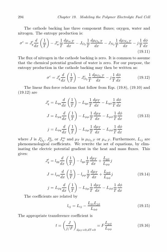
294 Chapter 19. Modeling the Polymer Electrolyte Fuel Cell
The cathode backing has three component fluxes; oxygen, water andnitrogen. The entropy production is:
σc = J ′q
d
dx
(1
T
)− Jc
w
1
T
dµw,T
dx− JO2
1
T
dµO2,T
dx− JN2
1
T
dµN2,T
dx− j
1
T
dφ
dx
(19.11)
The flux of nitrogen in the cathode backing is zero. It is common to assumethat the chemical potential gradient of water is zero. For our purpose, theentropy production in the cathode backing may then be written as:
σc = J ′q
d
dx
(1
T
)− Jc
O2
1
T
dµO2,T
dx− j
1
T
dφ
dx(19.12)
The linear flux-force relations that follow from Eqs. (19.8), (19.10) and(19.12) are
J ′q = Lqq
d
dx
(1
T
)− Lqµ
1
T
dµT
dx− Lqφ
1
T
dφ
dx
J = Lµqd
dx
(1
T
)− Lµµ
1
T
dµT
dx− Lµφ
1
T
dφ
dx
j = Lφqd
dx
(1
T
)− Lφµ
1
T
dµT
dx− Lφφ
1
T
dφ
dx
(19.13)
where J is JcO2, Ja
D, or Jmw and µT is µO2,T or µw,T . Furthermore, Lij are
phenomenological coefficients. We rewrite the set of equations, by elim-inating the electric potential gradient in the heat and mass fluxes. Thisgives:
J ′q = lqq
d
dx
(1
T
)− lqµ
1
T
dµT
dx+Lqφ
Lφφj
J = lµqd
dx
(1
T
)− lµµ
1
T
dµT
dx+Lµφ
Lφφj
j = Lφqd
dx
(1
T
)− Lφµ
1
T
dµT
dx− Lφφ
1
T
dφ
dx
(19.14)
The coefficients are related by
lij = Lij −LφiLjφ
Lφφ(19.15)
The appropriate transference coefficient is
t =
(J
j/F
)
dµT =0,dT=0
= FLµφ
Lφφ(19.16)

19.3. The electrode backing and the membrane 295
The Peltier coefficient is
π =
(J ′
q
j/F
)
dµT =0,dT=0
= FLqφ
Lφφ(19.17)
and the measurable heat of transfer
q∗ =
(J ′
q
J
)
j=0,dT=0
=lqµ
lµµ(19.18)
We introduce these definitions into the last set of flux equations, solvethe expression for the gradient in chemical potential, and introduce theexpression for dµT /dx into the heat flux. Equation 19.14 becomes
dT
dx= − 1
λ
[J ′
q − q∗(J − t
j
F
)− π
j
F
]
dµT
dx= −q
∗
T
dT
dx− 1
lµµ
(J − t
j
F
)
dφ
dx= − π
TF
dT
dx− t
F
dµT
dx− rj
(19.19)
where the stationary state thermal conductivity, λ, the mass transfer coef-ficient lµµ (on a mole fraction basis) and the resistivity r are:
λ =lqq
T 2− (q∗)2
lµµ
T 2
lµµ =Dx
RT
r = T/Lφφ
(19.20)
Here, D is the appropriate diffusion coefficient and r is the electric resis-tivity. The variables have their specific meaning in the various subsystemsof the cell, and this shall be specified below.
19.3.2 The anode backing
The anode backing has transport of heat, hydrogen, water and charge.Hydrogen and water are transported in the pores of the backing at constantpressure, p. The transport of charge and heat takes place in the solidmaterials of the backing. We introduce the expression for the chemical

296 Chapter 19. Modeling the Polymer Electrolyte Fuel Cell
potential of water µ = µ0 +RT lnxw/x∗w, where x∗w is the mole fraction at
saturation. The result is
dT
dx= − 1
λa
[J ′a
q + q∗,a
(Ja
D − taDj
F
)+ πa j
F
]
dxw
dx= −q
∗,axw
RT 2
dT
dx− 1
DwH
(Ja
D − taDj
F
)
dφ
dx= − πa
TF
dT
dx− taDRT
Fxw
dxw
dx− raj
(19.21)
Equation (19.21a) has three contributions to the temperature gradient.When the current density is large, the last contribution is significant com-pared to the Fourier type contribution and the contribution from the waterflux. Likewise, there is a contribution to the gradient in the mole fractionof water from the temperature gradient, but this contribution is not signif-icant in magnitude. The electric potential gradient does not only have anohmic contribution, −raj. The other two contributions here are small, butthey are needed to satisfy the second law.
The mole fraction of water is calculated from the partial pressure ofwater and the total pressure, xw = pw/p
0. At the left side boundary,the mole fraction is x0
w = p∗,aw /p0, given by the saturation pressure at
the temperature of this location, p∗(T a). The three main coefficients andthe three coupling coefficients characterize the transport of heat, mass andcharge through the backing. The Peltier heat of the anode is:
πa
T= −1
2SH2
− S∗e− (19.22)
where the transported entropy of electrons in carbon, S∗e− , is −2 J/K [190].
In Sec. 19.5, we show that a possible choice for the heat of transfer of wateris:
q∗,a = −TSaw (19.23)
The six transport coefficients for the anode backing were used to solveEqs. (19.21) and the energy balance:
d
dxJu =
d
dxJ ′a
q + jdφ
dx+ JH2
dHH2
dx+ Ja
w
dHw
dx= 0 (19.24)
Here, Ju is the constant energy flux through the backing, and dHi/dx =Cp,i (dT/dx). The equations were solved with boundary pressures for hy-drogen and oxygen of p = 1, 013× 105 Pa and 0.21p, respectively. Temper-atures at the boundaries were 340 K. The outcome of the calculation forall five subsystems is illustrated in Figs. 19.2, 19.3 and 19.4.

19.3. The electrode backing and the membrane 297
Figure 19.2 The temperature profile across the cell as a function of currentdensities 500, 2500 and 5000 A/m2. The highest current density gives thehighest curves.
Figure 19.3 The mole fraction profile of water (left) and oxygen (right) as afunction of current densities 500, 2500 and 5000 A/m2. The highest currentdensity gives the lowest curve.

298 Chapter 19. Modeling the Polymer Electrolyte Fuel Cell
Figure 19.4 The electric potential profile across the cell as a function of cur-rent densities 500, 2500 and 5000 A/m2. The highest current density gives thelowest curve.
The temperature profile in the anode backing has a negative slope inFig. 19.2, meaning that the coupling terms dominate since the heat fluxis negative. The mole fraction profiles show a sinking concentration ofwater on the left hand side in Fig. 19.3. The higher the current density, thebigger is the slope of this profile. There is a negligible change in the electricpotential in the backing in Fig. 19.4, corresponding to a small resistivity,small temperature differences and a relatively small variation in chemicalpotential of hydrogen. We return to the figures when we describe the othersections of the cell.
19.3.3 The membrane
The transport equations (19.19) for the membrane are:
dT
dx= − 1
λm
[J ′,m
q − q∗,m(Jmw − tmw
j
F) − πm j
F
]
dµw,T
dx= −q
∗,m
T
dT
dx− 1
lmµµ
(Jm
w − tmwj
F
)
dφ
dx= − πm
TF
dT
dx− tmwF
dµw,T
dx− rmj
(19.25)

19.3. The electrode backing and the membrane 299
with the stationary state thermal conductivity λm, the electric resistivityrm, the water transference number tmw , and the diffusion coefficient of waterin the membrane (on a concentration basis):
lmµµ = Dmw
cwRT
See Table 19.2 for coefficient values. The water activity in the membrane iscalculated from its definition, aw = pw/p
∗w. We have assumed that there is
equilibrium for water at the electrode/membrane interface, and that thereare no significant pressure gradients within the membrane [250]. The waterin the membrane is not in an ideal solution. The experimental relationbetween the water activity and the membrane water content is [251]:
λ(aw < 1) = 0.043 + 17.81aw − 39.85a2w + 36.0a3
w
λ(1 < aw < 3) = 14 + 1.4aw
λ(aw > 3) = 16.8
(19.26)
where the water content λ is the mole water per mole membrane ionic site:
λ = cwM/ρ (19.27)
Here, M is the molar mass of the polymer in the membrane, and ρ isthe membrane dry density. At the cathode side of the membrane, we useac
w = 1. The mass flux becomes:
Jmw = −q
∗,mDmw λρ
RMT 2
dT
dx− Dm
w ρ
M
dλw
dx+ tmw j/F (19.28)
We replace dλ/dx by (dλ/daw)(daw/dx) and solve for daw/dx, and usingdλ/daw from Eq. (19.26), the differential equations become:
dT
dx= −
J ′mq
λm+q∗,m
λm
(Jm
w − tmwj
F
)+πmj
λmF
daw
dx= − q∗,mλ
(dλ/daw)RT 2
dT
dx− (Jm
w − tmw j/F )M
(dλ/daw)ρDmw
dφ
dx= − πm
TF
dT
dx− tmwRT
Faw
daw
dx− rmj
(19.29)
The Peltier coefficient for the membrane is:
πm
T= S∗
H+ − tmwSmw (19.30)

300 Chapter 19. Modeling the Polymer Electrolyte Fuel Cell
We take an expression for the heat of transfer q∗,m similar to that in theanode:
q∗,m = −TSmw (19.31)
The electric resistivity, rm was given by Springer et al. [251]:
(rm)−1 = exp
(1268
(1
303− 1
T
))(0.5139λ− 0.326) (19.32)
The membrane diffusion coefficient Dm = 1.5 × 10⁻¹⁰ m2s was also givenby Springer et al. [251]. For the thermal conductivity of the membrane,we used an estimate for a water filled polymer, λm = 0.2 W/K m [246].The membrane density and molar mass were 1.64 kg/m3 and 1.1 kg/mol,respectively. The water transference coefficient of water in Nafion 115 inequilibrium with vapor was 1.2 [157]. The πm/Tm,c was taken from theliterature [252].
Energy conservation in the membrane means that, cf. Eq. (4.16),
d
dxJu =
d
dx(J ′m
q + jφm + Jmw H
mw ) = 0 (19.33)
The equations were solved to give the gradient in electric potential, thetemperature and concentration profiles across the membrane, see Figs. 19.2through 19.4.
The non-linear electric potential profile in the membrane, shown inFig. 19.4, can be understood from these properties. As the membranewater content goes down at the anode surface, the resistance increases, andso does the potential drop. This is the biggest contribution to the electricpotential gradient across the membrane. The contribution from the waterchemical potential is not big, since we assume equilibrium for water at bothelectrode surfaces. The temperature may rise or fall, depending on j. Achanging value of jφm, leads indeed to a change in J ′m
q , see Fig. 19.5 below.
19.3.4 The cathode backing
The flux equations (19.19) for the cathode backing are
dT
dx= − 1
λc
[J ′c
q + πc j
F
]
dxO2
dx=
j
4FDON
dφ
dx= −π
c
F
dT
dx− RT
4FxO2
dxO2
dx− rcj
(19.34)

19.4. The electrode surfaces 301
where we introduced tO2= 1/4 and neglected coupling between the oxygen
and other gas fluxes. The stationary state thermal conductivity is λc, andthe electric resistivity is rc. The oxygen concentration gradient is deter-mined by the interdiffusion coefficient of oxygen in nitrogen, by DON . ThePeltier coefficient for the cathode backing is:
πc
T=
1
4SO2
− S∗e − tcwS
cw =
1
4SO2
− S∗e −
(Ja
w
j+
1
2
)Sc
w (19.35)
The Peltier coefficient includes an extra contribution from water. Energyconservation in the cathode backing means that
d
dxJu =
d
dx(J ′c
q + jφc + JcwH
cw + JN2
HN2+ JO2
HO2) = 0 (19.36)
where dHi/dx = CP,idT/dx. These equations were solved for the profilesof T, xw and φ in the cathode. The equations were solved with a molefraction of oxygen at the right side boundary equal to x0
O2= pO2
/p = 0.21,see Figs. 19.2, 19.3 and 19.4. The consumption of oxygen is proportionalto j. The diffusion coefficient DON therefore determined the mole fractionprofile of oxygen in the cathode backing. The temperature profile indicatesa large heat flux out of the cell. In fact, most of the heat produced in thecell comes out of the cathode. Again, the electric potential gradient wasnegligible.
19.4 The electrode surfaces
The entropy production of the electrode surfaces between the i-phase andthe o-phase is:
σs = J ′iq ∆i,s
(1
T
)+ J ′o
q ∆s,o
(1
T
)− J i
w
1
T s∆i,sµw,T − Jo
w
1
T s∆s,mµw,T
− j1
T s
(∆i,oφ+
∆nGs
F+
∆µg,T
vgF
)(19.37)
The first superscript indicates the phase, and the second the position inthe phase. Superscript i means into (the left hand side of) the surface,while o means out (the right hand side) of the surface. For terminology,see Secs. 9.1 and 13.1. (The excess entropy production in the anode andcathode surfaces, in J/s K m2, are σs,a and σs,c.) There is a discontinuityin the heat flux at the surface; we distinguish between the flux into thesurface, J ′i
q , and out of the surface, J ′oq . This can be seen in Fig. 19.5

302 Chapter 19. Modeling the Polymer Electrolyte Fuel Cell
below. The last term comes from transport of the reacting gas into thesurface. The force-flux relations are:
∆i,s
(1
T
)= rs
iiJ′iq +rs
iµJiw+rs
ioJ′oq +rs
imJow+rs
iφj
− 1
T s∆i,sµw,T = rs
µiJ′iq +rs
µµJiw+rs
µoJ′oq +rs
µmJow+rs
µφj
∆s,o
(1
T
)= rs
oiJ′iq +rs
oµJiw+rs
ooJ′oq +rs
omJow+rs
oφj
− 1
T s∆s,oµw,T = rs
miJ′iq +rs
mµJiw+rs
moJ′oq +rs
mmJow+rs
mφj
− 1
T s
(∆φ+
∆nGs
F+
∆µg,T
vgF
)= rs
φiJ′iq +rs
φµJiw+rs
φoJ′oq +rs
φmJow+rs
φφj
(19.38)We assume that rs
io = rsoi = 0, and rs
im = rsmi = 0. It follows that:
J ′iq =
rsµµ
Diµ∆i,s
(1
T
)−
rsiµ
Diµ
(− 1
T s∆i,sµw,T
)+ πi j
F
J iw = −
rsµi
Diµ∆i,s
(1
T
)+
rsii
Diµ
(− 1
T s∆i,sµw,T
)+ ti
j
F
J ′oq =
rsmm
Dom∆s,o
(1
T
)− rs
om
Dom
(− 1
T s∆s,oµw,T
)+ πo j
F
Jow = − rs
mo
Dom∆s,o
(1
T
)+
rsoo
Dom
(− 1
T s∆s,oµw,T
)+ to
j
F
(19.39)
where the denominators are
Diµ = rsiir
sµµ − rs
iµrsµi
Dom = rsoor
smm − rs
omrsmo
(19.40)
and the transference numbers and Peltier coefficients are
tiw = F
(J i
w
j
)
dT=0,dµ=0
= Frsiφr
sµi − rs
iirsµφ
Diµ
tow = F
(Jo
w
j
)
dT=0,dµ=0
= Frsoφr
smo − rs
oorsmφ
Dom
(19.41)

19.4. The electrode surfaces 303
πi = F
(J ′i
q
j
)
dT=0,dµ=0
= Frsµφr
sµi − rs
µµrsiφ
Diµ
πo = F
(J ′o
q
j
)
dT=0,dµ=0
= Frsmφr
smo − rs
mmrsoφ
Dom
(19.42)
These coefficients are equal to the coefficients that were defined for the bulkphases. The heats of transfer from the linear relations are:
q∗,i = −rsiµ
rsii
q∗,o = −rsom
rsoo
(19.43)
By introducing these ratios, we obtain expressions for the jump in temper-ature and in chemical potential at the surface:
∆i,sT = − 1
λsi
[J ′i
q − q∗,i
(J i
w − tiwj
F
)− πi j
F
]
∆i,sµw,T = − q∗,i
T i,o∆i,sT − T s
liµµ
(J iw − tiwj/F )
∆s,oT = − 1
λso
[J ′o
q − q∗,o
(Jo
w − towj
F
)− πo j
F
]
∆s,oµw,T = − q∗,o
T o,i∆s,oT − T s
loµµ
(Jo
w − towj
F
)
(19.44)
Here, λsi and λs
o are stationary state thermal conductivities of the i ando side of the surface, respectively, and liµµ and loµµ are corresponding sta-tionary state mass conductivities. The heat fluxes have a Fourier-typecontribution as well as a contribution from the Peltier heat and the heat oftransfer.
The effective electric force becomes:
∆i,oφeff = ∆i,oφ+∆nG
s
F+
∆µg,T
vgF
= − πi
T i,oF∆i,sT − πo
T o,iF∆s,oT − tiw
F∆i,sµw,T − tow
F∆s,oµw,T − rsj
(19.45)
where rs is the ohmic surface resistivity. The electric potential drop atthe surface has contributions from the Peltier coefficients, the chemical

304 Chapter 19. Modeling the Polymer Electrolyte Fuel Cell
potential difference, the reaction Gibbs energy, and the resistance dropacross the surface.
These equations capture the most important phenomena at the electrodesurfaces. They are further detailed below. It is remarkable that the fluxesare analogous to their bulk counterparts.
19.4.1 The anode catalyst surface
At the anode catalyst surface, the enthalpy of hydrogen is converted intoelectric energy and heat. There is a change in the enthalpy as water goesfrom the vapor state to the condensed state in the membrane. This releasesheat. Conservation of energy across the phase boundary means that
Ju = J ′aq + jφa + JH2
HH2+ Ja
wHaw = J ′m
q + jφm + Jmw H
mw (19.46)
The flux of hydrogen stops at the surface, while the electric current densityand the water flux are continuous through the surface:
Jaw = Jm
w . (19.47)
The difference in the electric potential between the two sides of the surfaceφm−φa = ∆a,mφ is generated by the heat and enthalpy changes. The heatfluxes in and out of the anode surface are illustrated in detail in Fig. 19.5for the same current densities and conditions as before.
We see a discontinuity in the heat flux at both electrode surfaces, and avarying heat flux in the membrane, for reasons we explained above. Nernstequation is obeyed when the entropy production is zero in an isothermalsurface, ∆a,mφ = −∆nG
s,a/F , see Sec. 5.4.1.The electrochemical reaction takes place at the surface, and the reaction
rate at stationary state is equal to j/F . We assume that there is equilibriumfor adsorption of hydrogen at the surface. This means that the reactionGibbs energy in the surface can be expressed by thermodynamic propertiesof the gas:
∆a,mφeff = ∆a,mφ+∆nG
s,a
F+
∆µH2,T (T s,a)
2F
= ∆a,mφ− 1
2F
(µs
H2− ∆a,sµH2,T (T s,a)
)
= ∆a,mφ− 1
2F(HH2
− T s,aSH2) (19.48)

19.4. The electrode surfaces 305
Figure 19.5 The heat fluxes in the cell as a function of current densities 500(unbroken line), 2500 (dotted curve) and 5000 (dashed curve) A/m2.
The equations of transport that derive from σs,a are:
∆a,sT = −J ′a
q
λsa
+q∗,a
λsa
(Jw − twj/F ) + πaj/λsaF
∆a,sµw,T = − q∗,a
T a,m∆a,sT − (Jw − twj/F )
lsµµ
∆s,mT = −J ′m
q
λsm
+q∗,m
λsm
(Jw − twj/F ) + πmj/λsmF
∆s,mµw,T = − q∗,m
Tm,a∆s,mT − (Jw − twj/F )
lsµµ
∆φeff = − πa
T a,mF∆a,sT − πm
Tm,aF∆s,mT − tw
F∆a,mµw,T − rsj
(19.49)
The conditions at the surface are not known in detail. In order to simplifymatter enough to make possible a calculation of the profiles of T, xw andφ across the cell, we assume that there is equilibrium for water across thesurface.

306 Chapter 19. Modeling the Polymer Electrolyte Fuel Cell
∆µw = (Haw − T aSa
w) − (Hmw − TmSm
w ) = 0 (19.50)
This relation may be used to find the temperature of the membrane, con-sistent with T a and the thermodynamic properties. The chemical potentialdifference at constant temperature, is then equal to
∆a,sµw,T (T s,a) = T s,a(Ssw − Sa
w)
∆s,mµw,T (T s,a) = T s,a(Smw − Ss
w)(19.51)
These equations, together with the energy balance and Eq. (19.50) weresolved for the temperature jumps and the electric potential drop at thesurface. The Peltier coefficients are known, while the thermal and massconductivities are not. Condition Eq. (19.50) is a useful replacement for theflux equations for ∆a,sµw,T and ∆s,mµw,T . Necessary coefficient estimateswere given in Table 19.2. For the anode surface resistivity, we used rs = 7.210−6 ohm m2. Vie [246] determined the thermal conductivity of the catalystsurfaces from experiments, λs = 1000 W/Km2 from a model similar to thisone, but without coupling terms.
Figure 19.4 gives a relatively large jump in the electric potential atthe anode surface, while Fig. 19.2 shows a small jump in the temperature.Both jumps are connected to the entropy change of the electrode reaction,Eq. (19.48).
19.4.2 The cathode catalyst surface
Energy conservation at the cathode surface gives
Ju = J ′mq + jφm + Jm
w Hmw
= J ′cq + jφc + (Ja
w + j/2F )Hcw + JO2
HO2(19.52)
The effective electric force becomes:
∆m,cφeff = ∆m,cφ+∆nG
s,c
F− ∆µO2,T
4F
= ∆m,cφ+1
2F(Hc
w − T s,cScw) − 1
4F(HO2
− T s,cHO2) (19.53)

19.5. A model in agreement with the second law 307
The potential jump across the surface is ∆m,cφ = φc − φm. The equationsto be solved for the profiles are:
∆m,sT = − 1
λsm
[J ′m
q − q∗,m
(Jm
w − tmwj
F
)− πm j
F
]
∆m,sµw,T = − q∗,m
Tm,c∆m,sT − 1
Lmµµ
(Jm
w − tmwj
F
)
∆s,cT = − 1
λsc
[J ′c
q − q∗,c
(Jc
w − tcwj
F
)− πc j
F
]
∆s,cµw,T = − q∗,c
T c,m∆s,cT − 1
lcµµ
(Jc
w − tcwj
F
)
(19.54)
We assume again equilibrium for water across the surface, cf. Eq. (19.50), aswell as equilibrium for oxygen adsorption at the surface. The Peltier heatsare the ones given before. The electric potential of the cell is generated atthe cathode. It can be calculated from
F (∆m,cφeff + ηc) = − πm
Tm,c∆m,sT − πc
T c,m∆s,cT
− tmw ∆m,sµw,T − tcw∆s,cµw,T − rsj (19.55)
The overpotential of the oxygen electrode, ηc, or the resistance of the acti-vated electrochemical reaction, is not yet accounted for. It can be shown,using mesoscopic non-equilibrium thermodynamics, that the overpotentialmust be subtracted from the right-hand side of Eq. (19.53) [51]. The valueof the cathode overpotential was determined by Vie and Kjelstrup [247]:
ηc =2RT
Fln
j
j0(19.56)
with the exchange current density for oxygen in air of j0= 2.5 10−3 A/m2.The resulting jump in electric potential is shown in Fig. 19.4.
19.5 A model in agreement with the second law
The entropy production for a unit cross-sectional area (Ω = 1m2) of thecell is the integral over contributions from all five subsystems:
dSirr
dt= Ω
[∫ a,m
0a
σadx+ σs,a +
∫ c,m
a,m
σmdx + σs,c +
∫ 0,c
c,m
σcdx
]≥ 0
(19.57)
where dSirr/dt has dimension W/K. The second law gives dSirr/dt > 0.

308 Chapter 19. Modeling the Polymer Electrolyte Fuel Cell
The entropy balance for the whole cell is:
dSirr
dt= [Jc
s − Jas ] Ω (19.58)
The entropy flux was defined in Sec. 4.2, Js = J ′q/T + ΣiJiSi. Here, J ′
q
is the measurable heat flux, Ji is the mass flux of component i, Si is thepartial molar entropy of i, and T is the temperature. These fluxes give
1
W
dSirr
dt=
(J ′c
q
T c+ Jc
wScw + JO2
SO2
)−(J ′a
q
T a+ Ja
wSaw + JH2
SS2
)
=J ′c
q
T c−J ′a
q
T c+j
F
[1
2(Sc
w − SH2) − 1
4SO2
]+ Ja
w [Scw − Sa
w]
(19.59)
The measurable heat fluxes have, as we have seen, several terms, not onlyFourier type terms. All terms are important in the development of a consis-tent thermodynamic model. In such a model, we must find the same valuefor the entropy production from Eq. (19.57) as from (19.59).
The entropy production was therefore determined by integrating acrossthe sections of the cell. The accumulated entropy production for the cellin Figs. 19.1–19.4 is shown in Fig. 19.6 for three current densities. Wesee, as expected, that most of the entropy is produced at the cathode.The entropy production increases with the current density in the cell. Theintegrated value agreed within numerical accuracy with the value calculatedfrom Eq. (19.59).
The cell was leaking heat to both sides, more to the cathode side,than to the anode side, see Fig. 19.5. A reduction in the overpotentialin the cathode surface had a substantial effect on σs,c and the heat fluxes.The thermal conductivities of the backing and surface were significant forthe temperature rise in the system, but not for the entropy production.The value of the diffusion coefficient for water in the membrane has a largeeffect on the possibility to find a solution. The membrane resistivity gavesignificant contributions to the entropy production.
In order to see the importance of coupling terms in the heat fluxes, weintroduce the heat fluxes from the subsections above. This gives
1
W
dSirr
dt= − λc
T 0
(dT
dx
)c
+πc
T
j
F
+λa
T 0
(dT
dx
)a
− q∗,a
T
(Ja
D − taDj
F
)− πa
T
j
F
+j
F
[1
2(Sc
w − SH2) − 1
4SO2
]+ Ja
w (Scw − Sa
w) (19.60)

19.5. A model in agreement with the second law 309
Figure 19.6 The accumulated entropy production in the polymer electrolytefuel cell, obtained by integration from the anode to the cathode backing, forcurrent densities 500 (lower curves), 2500 (central curves) and 5000 (uppercurves) A/m2.
The next step is to introduce the expressions for the Peltier coefficients(19.22) and (19.35), and the relation for the anode Ja
D − taDj/F = Jaw. Part
of the difference of the Peltier coefficients then cancel with the entropy ofthe reaction. This is so because the heat effect connected with conversionof reactants to products, does not contribute to the entropy production,but to the electric work. The terms containing the heats of transfer arereversible, and must not give any net entropy production. This is achievedwhen
q∗,a = −TSaw (19.61)
andq∗,c
T− q∗,a
T= −Sc
w + Saw (19.62)
With these relations, we also have
1
W
dSirr
dt= − λc
T 0
(dT
dx
)c
+λa
T 0
(dT
dx
)a
(19.63)
The total entropy production in the cell ends up as heat conducted to thesurroundings in this model.

310 Chapter 19. Modeling the Polymer Electrolyte Fuel Cell
19.6 Concluding comments
We have demonstrated how non-equilibrium thermodynamics can be usedto characterize energy conversion in a polymer fuel cell. The method canbe used for any heterogeneous electrochemical cell. We have presenteda set of simultaneous solutions for mole fractions, electric potentials andtemperature profiles across a single polymer electrolyte fuel cell using datafor a Nafion 117 membrane. From the solutions, we have calculated the localentropy production in each subsystem of the cell in two ways. We foundthat heat may escape the cell in an asymmetric manner, largely dependenton the thermal conductivity of the surfaces. The calculations were done fora one-dimensional cell.
Knowledge of entropy production, lost work and local heat fluxes isimportant for auxiliary equipment design and for further research planning.The largest reduction in entropy production, or increase in power output,can be obtained by reducing the overpotential of the cathode, but it isworthwhile paying more attention also to the membrane as a dissipatingpart of the cell.

Chapter 20
Measuring Membrane
Transport Properties
Non-equilibrium thermodynamics can be used to design experiments. Wepresent methods and experimental results that have been obtained withcation-exchange membranes.
Membranes are widely used to separate mixtures of all kinds. A mem-brane can be generally seen as a barrier to transport. Biological membranesseparate the interior of a cell from its exterior, or organelles from the cellinside. Inorganic and organic membranes selectively conduct ions, for in-stance, in ion-selective electrodes, and can be used as sensors. Clay andsand can be used to filter impurities from drinking water, and can also bethought of as membranes in a wide sense.
Non-equilibrium thermodynamics has since long been used to describetransport in membranes [23, 24, 227, 230, 250, 253–255]. The theory needsinput values for transport coefficients, in order to be used for modeling.When such coefficients are not known, experiments can be designed tomeasure them, using the same theory.
This chapter describes experimental methods which can be used to findtransport properties for ion-exchange membranes [27,77,157,239,256–258].The methods, which are designed from the theoretical framework, may alsobe used for other membranes. We shall illustrate them with data for ion-exchange membranes. We saw that ion-exchange membranes were used forenergy conversion in fuel cells (Chapter 19) and in osmotic power plants(Chapter 18). They are also used to separate salt solutions and to produceclean water [229].
The cells reported are of the type
Ag(s)|AgCl(s)|NCl, ACl (aq)|mem| NCl, ACl (aq)|AgCl(s)|Ag(s) (20.1)
311

312 Chapter 20. Measuring Membrane Transport Properties
The aqueous solution contained up to two chlorides, NCl and ACl. Themembranes were cation exchange membranes, the CR membrane was fromIonics and the Nafion 117 membrane, from Dupont. The electrodes werereversible to the ion in solution, Ag(s)| AgCl(s) or (Pt)|H2(g).
20.1 The membrane in equilibrium with electrolyte solutions
Equilibrium constants for membrane-electrolyte equilibria can be calcu-lated from measurements of membrane compositions and their correspond-ing electrolyte compositions. This was done for some selected electrolytemixtures in equilibrium with the CR membrane from Ionics [235,236]:
HCl + NaM HM + NaCl Keq,1 =aHMaNaCl
aHClaNaM= 0.72
NaCl + KM NaM + KCl Keq,2 =aNaMaKCl
aNaClaKM= 0.54 (20.2)
SrCl2 + KM SrM2 + KCl Keq,3 =aKClaSrM2
aKMaSrCl2
= 5.6
Here, M− denotes a cation site in the membrane. The ion exchange capacityof the CR 386 membrane is 1.6 kmol m−3 and the membrane is 1.2 µm thick.The equilibrium constants show that the membrane has a small preferencefor HM over NaM, a very small preference for NaM over KM, and a highpreference for SrM2 over KM. When the equilibrium constant is close tounity, the cations are nearly statistically distributed over the cation sites inthe membrane. The higher value for the mixture of SrM2 and KM indicatesthat the divalent ion binds to more than one site.
The path of transport through a membrane is everywhere at local equi-librium. The path can thus be defined also by means of solutions that arein equilibrium with the membrane at any given location between the twosides. This is convenient when one needs to integrate across a membrane.
20.2 The membrane resistivity
Ion-exchange membranes are normally good conductors. It is thereforedifficult to separate the membrane resistance from the resistance of adjacentlayers. The membrane resistivity can therefore best be found by measuringa stack of several membranes [157, 259]. The single membrane pieces arefirst equilibrated in the electrolyte. The membranes are pressed togetherbetween two electrodes. A constant pressure is applied. For an isothermal

20.2. The membrane resistivity 313
Figure 20.1 The resistance of a stack of CR Ionics membranes, R(n), as afunction of the number of membranes in the stack, n [157]. The membraneswere equilibrated in various solutions of HCl.
stack of uniform composition, the ohmic resistance is
R = −(
∆φ
I
)
dT=0,dµi=0
(20.3)
The total cell potential, ∆φ, is measured at a high frequency, in order toavoid frequency dependent phenomena (see Chapter 21). The cell resis-tance, R(n), is then
R(n) = Ro + nRms (20.4)
where Ro is the resistance of the wires and the liquid layers at the elec-trodes, n is the number of membranes and Rms is the resistance of onemembrane, Rm, and a surface layer, Rs:
Rms = Rm +Rs (20.5)
A plot of R(n) versus n gives a straight line, see Fig. 20.1 which shows datafor HCl in Nafion 117. The slope of the line gives Rms.
The membrane resistance and the surface resistance can be separated,assuming that Rs depends on the electrolyte concentration, while Rm doesnot. When the surface resistance is proportional to the specific resistivityof the solution, ρ, we can find Rm by plotting Rms versus ρ. This plot is

314 Chapter 20. Measuring Membrane Transport Properties
Figure 20.2 The resistance of a single CR Ionics membrane with interfacelayer, Rms, as a function of the resistivity, ρ, of the KCl solution in equilibriumwith the membrane [157].
shown in Fig. 20.2. The surface resistance Rs is more than 10% of Rm forHCl in equilibrium with CR 386 from Ionics [157,259].
The deviation from the straight line at high concentrations in Fig. 20.2was explained by membrane swelling [157, 259]. The membrane specificresistivity can now be found from Rm, the membrane area, Ωm, and themembrane thickness, dm:
rm = Rm
(Ωm
dm
)(20.6)
Results for the membranes were κm = 1/rm = 0.420 ±0.04 (CR 386) and2.03 ±0.04 S/m (Nafion 117). The technique was used to find specificconductivities for mixtures of monovalent cations, and mixtures of mono-and divalent cations.
The conductivity can be modeled with a formula similar to the one givenin Sec. 16.1
κm = −[∆φ
j
]
dT=0, dµi,T =0
= F 2c (uN+xNM + uA+xAM) (20.7)

20.2. The membrane resistivity 315
Table 20.1 Cation mobilities in Nafion and Ionics CR. The mobility hasdimension 108 m2/Vs and refers to 298 K.
Cation(uo
+
)∞
Nafion 117 Ionics CR386
H+ 36.3 14.8 2.30Na+ 5.19 2.7 0.30K+ 7.61 – 0.38
Ca2+ 6.16 2.5 –Sr2+ – – 0.09
where c is the concentration of cation sites in the membrane, and xi is theequivalent fraction of ion i in the membrane. Some ion mobilities are givenin Table 20.1 for one cation in Nafion 117 and Ionics CR386. Mobilitiesin Nafion 117 are approximately half the values in infinitely dilute aqueoussolutions,
(uo
+
)∞
. With xAM+ xNM = 1, we eliminate xNM in Eq. (20.7),and obtain
κm = F 2c [(uA+ − uN+)xAM + uN+ ] (20.8)
Mobilities of ions in dilute aqueous solutions are essentially constant. Equa-tion (20.6) predicts that κ is a linear function of xM+ , if the membranemobilities are constant. This was not observed, and the following modelwas proposed:
uA+ = uoA+(1 − kxNM)
uN+ = uoN+(1 − kxAM)
(20.9)
Here, uoA+ and uo
N+ are the mobilities of AM and NM respectively, andk is an empirical constant describing the interaction of ions. The con-stant expresses how likely it is that the movement of one ion is obstructedby movement of the other. Conductivity data from several investiga-tors [157, 235, 260, 261] were fitted to this model. Results are given inTable 20.2. A zero interaction constant was found in the presence of pro-tons. It seems likely, considering the amount of water present in the mem-branes (40-50w%), that the transport mechanism of protons is differentfrom that of other ions. The mobility ratio is smaller in the membranethan in a dilute solution. The membrane serves to retard the fast ion, andto accelerate the slow ion. This seems likely for a membrane, where ex-change of ions between the sites is important. The ionic mobilities can be

316 Chapter 20. Measuring Membrane Transport Properties
Table 20.2 Mobility ratios and interaction constants for cations. The mem-brane is CR 386 from Ionics. Results are compared to infinitely dilute aqueoussolutions.
Cation pair(uo
A+/uoN+
)M−
k(uo
A+/uoN+
)∞
Reference
H+/Na+ 4.2 ± 0.2 0 7.0 [157]H+/K+ 4.9 ± 0.1 0 4.8 [157]Na+/K+ 0.97 ± 0.03 0.16 ± 0.06 0.68 [260,261]K+/Sr2+ 4.2 0.28 – [235]
used to estimate ionic transport numbers from
tA+ =
(JACl
j
)
dT=0,dµi=0
=uo
A+(1 − kxNM)
κ/cF 2
tA+ =
[1 +
uoN+(1 − kxAM)
uoA+(1 − kxNM)
xNM
xAM
]−1(20.10)
and tN+ = 1−tA+ . These transport numbers were confirmed by independentmeasurements for membranes with protons [27], see Sec. 20.3. For alkali-metal mixtures the following approximation was good [260,261]
tA+ ≈ xAM (20.11)
The last situation is compatible with uoA+(1−kxNM) ≈ uo
N+(1−kxAM). Themembrane transport number can thus, in the simplest case, be determinedfrom knowledge of membrane composition alone.
20.3 Ionic transport numbers
Ottøy et al. [257] developed a technique to determine the transport numberin a two-component mixture as continuous function of composition. A stackof membranes was used. The stack had so many membranes (usually 8 to10) that the boundary solutions were not changed during the experiment(by diffusion). Half of the stacks were equilibrated in a reference solution,the other half in the test solution. In this manner, he was able to find theconcentration dependent transport number.
Consider again the membrane in equilibrium with KCl and HCl in cell(20.1). Experiments were performed at constant pressure, constant tem-perature and constant chemical potential of water, that is, the electrolytesolutions had the same ionic strength. The reference solution was put on

20.3. Ionic transport numbers 317
Figure 20.3 The electric potential difference in cell 20.1 as a function of[µc
HCl − µcKCl]. Reproduced from J. Membr. Sci. 74 (1992) 1–8 with permission
from Elsevier.
the left hand side, and the test solution was put on the right hand side.The gradient in the electric potential became
(dφ
dx
)
j=0,dT=0,dµw=0
= −tHMdµc
HCl
dx− tKM
dµcKCl
dx(20.12)
The transport of KCl across the membrane, is everywhere defined by thetransport of K+. The transference number of KCl is therefore equal to thetransport number of K+, tKM = tK+ , with the membrane as the frame ofreference. In evaluating the transport of HCl, the electrode reactions mustbe accounted for. In the absence of KCl, there is no net mass transportby charge transport alone, and tHM = 0. In the presence of KCl, as it ishere, mass balances give a net transfer of HCl, opposite in sign, but equalin magnitude to the flux of KCl. The transference coefficient of HCl istherefore tHM = −tK+ . This gives
tK+ =dφ
d [µcHCl − µc
KCl](20.13)

318 Chapter 20. Measuring Membrane Transport Properties
Figure 20.4 The transference number of H+ as a function of membrane com-position xHM for the systems KM-HM and NaM-HM. Reproduced from J.Membr. Sci. 74 (1992) 1–8 with permission from Elsevier.
The differentials of the variables can be related to differentials of differences,since we keep the reference solution constant:
tK+ =d∆φ
d∆[µcHCl − µc
KCl](20.14)
The composition on the left hand side of the stack is varied in the experi-ment. By plotting the potential difference as a function of ∆[µHCl − µKCl] ,we can find the transference number from the tangent to the curve in anypoint (any composition) on the curve. An example of such a curve is shownin Fig. 20.3. Results for two systems are presented in Fig. 20.4.
The measured transport number was compared to the results calcu-lated from the mobility model above, Eq. (20.8). Agreement was foundwithin the experimental uncertainty (3% for HM-KM and HM-NaM). Cellpotentials can be measured with high precision when j = 0. Such emfmeasurements can be used to give accurate transport numbers, betterthat numbers obtained from the Hittorf method. The problem, which isto find the concentration dependence of the transport number, can alsobe solved.

20.4. The transference number of water and the water permeability 319
20.4 The transference number of water and the
water permeability
The water transference number, tw, gives the number of water moleculestransported with the electric current in the membrane. According to thedefinition;
tw =
(Jw
j/F
)
dT=0,dµi=0
(20.15)
The transference number of water can be found in several ways. For a cationmembrane in a proton form, some authors use the potential difference ofthe following isothermal cell [157, 262]:
(Pt)H2(g)|H2O(g, a1w) |mem|H2O (g, ar
w)|H2(g)(Pt) (20.16)
The membrane was equilibrated prior to the experiment in HCl. The mem-brane was then put in contact with saturated vapor only; the activity ofwater in the vapor was controlled by the temperature and by the amountof LiCl in a water solution that was in equilibrium with the vapor. Thepotential difference across the membrane is:
(∆φ)j=0 = −twRT lnarw
alw
(20.17)
The difference in chemical potential of water across the membrane wasapplied, keeping al
w constant. By plotting ∆φ versus ln arw/a
lw, a linear
relation was found, see Fig. 20.5. The transference number is thereforeconstant. The value 1.2 was obtained for Nafion 117 at 298 K. Whenthe membrane is equilibrated with electrolyte solutions, the equilibrium isshifted towards higher water contents, and the water transference numberrises to 2.6 [263].
The water transference number for a membrane in contact with liquidsolutions, can also be accurately determined from the streaming potential[258]. An additional advantage with this measurement is that the waterpermeability can also be obtained. The streaming potential experiments aredone with constant temperature and concentration in the cell. A pressuredifference is applied across the membrane. It is assumed that the pressuregradient is linear in the membrane, with dp/dx = ∆p/dm.
The streaming potential of Cell (20.1) is[∆φ
∆p
]
dT=0,dµci=0
= −tAClVACl − tNClVNCl − twVw − ∆Vel (20.18)
When the transference numbers of the electrolytes have been determined(see Sec. 20.3), and the volume difference of the electrode reactions is cor-rected for ∆Vel = VAg − VAgCl, the unknown tw can be found.

320 Chapter 20. Measuring Membrane Transport Properties
Figure 20.5 The emf of cell 20.1 as a function of ln arw/a
lw at 298 K [157].
Several systems have been investigated for tw [260,264]. For monovalentcation mixtures, a model for tw is
tw = rA+tA+ + rN+tN+ = (rA+ − rN+) tA+ + rN+ (20.19)
with constant coefficients rA+ and rN+ . A linear variation in tw with tA+
may mean that a constant number of water molecules is carried with eachion. For membrane mixtures of divalent and mono-valent cations, the modelfails. The number of water molecules carried with each ion may then varywith the composition. The water transference number is largely reduced,and may even become negative, if the membrane becomes permeable toanions. The presence of an anion will add a negative term to Eq. (20.19).This straightforward interpretation of the water transference number as thesum of water molecules carried with each type of ion, is probably oversim-plified. It is known that the dynamics of water in the pore varies largelywith the ionic sites and the counter-ions that are present. The values ofrA+ and rN+ are not equal to the waters of hydration [259]. Membranehydrophobicity will increase tw.
Typical results from a streaming potential measurements are shown inFig. 20.6. The curves are extrapolated to zero time, t = 0, to determine thestreaming potential. We see that the potential difference across the cell, fora given pressure difference, is a linear function of
√t on a scale of seconds.
This behavior can be predicted. The pressure difference leads to a volumeflux, which is superimposed on the electro-osmotic flux. The volume flux

20.4. The transference number of water and the water permeability 321
Figure 20.6 The variation in the emf due to a pressure difference, as a functionof
√t. (Courtesy of T. Okada).
leads to a dilution of the solution on the receiving side, and a concentra-tion of the solution on the donating side. The presence of concentrationgradients on both sides of the membrane adds to the potential difference(20.18) as time goes on. When the solution contains only one electrolyte,the addition is [258]
∆φpol = −Lp8RT
√t√
πD1
∆p (20.20)
where D1 is Fick’s diffusion constant for diffusion of electrolyte in water,Lp is the membrane hydraulic permeability
Lp = −(JV
∆p
)
dT=0,dµci=0
(20.21)
and JV is the volume flux. For cells with one electrolyte, JV = J1V1 +JwVw + j∆Vel. By plotting the observed potential (∆φ+∆φpol) versus
√t,
the streaming potential is obtained by extrapolation to t = 0, and Lp isobtained from the slope of the curve.
The water permeability was found in this manner for NaM and SrM2
in the Ionics membrane. It was 2.4 and 0.9×10⁻¹⁴ m2/kgs respectively.The water permeability in Nafion membranes were larger by a factor 50.The value did not compare well with the diffusion coefficient for waterobtained for uniform pressure. This indicates that the pressure difference

322 Chapter 20. Measuring Membrane Transport Properties
Figure 20.7 Schematic drawing of the thermocell apparatus. Numbers de-fine 1) the N2 gas supply and 2) bubble flasks, 3) electrode compartments,4) Nafion membrane stack, 5) multispeed pumps, 6) Ag|AgCl-electrodes, 7)thermocouples, 8) potentiometer and 9,10) water baths. Reproduced from J.Membr. Sci. 107 (1995) 219–228 with permission from Elsevier.
may lead to viscous transport phenomena in nanometer (nm) small pores.Convective behavior has been observed in molecular dynamics simulationsfor pore diameters as small as a few molecular diameters [265].
20.5 The Seebeck coefficient
By measuring the thermoelectric potential, one can find the Peltier heat ofthe membrane. An apparatus for this measurement is shown in Fig. 20.7.Again, a membrane stack can be used. In this case, the temperature gradi-ent is controlled by the stack. The variation in the thermoelectric potentialis shown in Fig. 20.8.
The potential variation follows the recording of the thermistor in the so-lution with the high temperature. Eventually a stationary state is reached.The ratio of the two quantities gives the Seebeck-coefficient. For a cell withHCl, the measurements gave [263]
(∆φ
F∆T
)
j=0,∆p=0
≡ −twSw + S∗H+ = 13 J/Kmol (20.22)
By introducing tw = 2.6 and Sw = 69.9 J/K mol into this equation, we findS∗
H+ = 195± 14 J/K mol. High values for transported entropies of protonsare known from other systems [205]. From measurements of the Seebeckcoefficient, one can calculate the Peltier heat.

20.6. Interdiffusion coefficients 323
Figure 20.8 The emf of the thermocell as a function of time, when a temper-ature difference ∆T is applied to the cell. Reproduced from J. Membr. Sci.107 (1995) 219–228 with permission from Elsevier.
20.6 Interdiffusion coefficients
Diffusion experiments were done in the cell [27, 256]
NaCl(xNaCl,I, aq), HCl(xHCl,I, aq)|mem|HCl(xHCl,II, aq) (20.23)
There are no electrodes in this cell, so ∆φ = 0, j = 0. NaCl is component 1,HCl is component 2, and water is component 3. With isothermal solutionsof constant ionic strength, ∆µ3 = 0 and ∆T = 0, the flux equations can berewritten as
J1 = −l11dµ1
dx− l12
dµ2
dx
J2 = −l21dµ1
dx− l22
dµ2
dx
(20.24)
Because the solutions are electroneutral, the salt transports must obeyJ1 + J2 = 0, when j = 0. Since the chemical potential gradients areindependent of each other, it follows that
l11 + l12 = 0 l21 + l22 = 0 (20.25)

324 Chapter 20. Measuring Membrane Transport Properties
Figure 20.9 The flux of NaCl across an Ionics CR membrane during stationarystate interdiffusion of Na+ and H+ [256]. The right hand side of the membranehas pure HCl, while the left hand side as a mixture of NaCl and HCl given bythe mole fraction xHCl,I.
so that the problem reduces to determination of one coefficient, l11
J1 = −l11d
dx(µ1 − µ2) (20.26)
The flux of NaCl to the right was measured as a function of xHCl,I in theleft hand side solution, see Fig. 20.9, where xHCl is the mole fraction ofHCl in the solution. The stationary flux is the same everywhere in themembrane. The sum of the cation mole fractions of Na+ and H+ is unityin the membrane as well as in the solutions. The membrane thickness dm,was measured from the left where x = 0 to the right where x = dm.
In order to relate l11 to the appropriate composition, consider first thecase that has cHCl,I = 0. The flux J1 is the maximum one in Fig. 20.9.There is a concentration profile of NaM in the membrane, starting frompure NaM on the left hand side, going to 0 on the right hand side, seeFig. 20.10.
The concentration of HCl is next increased to x′HCl,I , and the flux islower, J ′
1. The value of the force at the inlet of the membrane is thesame as in the first case, not at x = 0, but at a position x′ from the

20.6. Interdiffusion coefficients 325
Figure 20.10 Expected concentration profiles across the membrane in the casethat xHCl,I = 0 (upper part of figure) and when it has changed to x′HCl,I (lowerpart of figure).
surface. Similarly, in the next measurement, the flux J ′′1 can be related
to the position x′′ in the first experiment where the value of the drivingforce is the same. Now, if the membrane was thinner in the second andconsecutive experiments, that is if it was dm − x′ in the second, dm − x′′ inthe third and so on numbered experiment, the values of the fluxes wouldhave been the same. Since the membranes all have the same thickness, thepositions with the same force must be related by
J ′1
J1=dm − x′
dm
This relation makes possible a determination of x′. But then we know thecomposition of the solution in equilibrium with the membrane at this po-sition. From the series of experiments we can then draw the concentrationprofile between 0 and dm. We can also draw a profile of chemical potentialsfor the two components through the membrane. This allows us to find theirgradients, the gradient difference, and finally the driving force for interdif-fusion. The calculation of l11 follows. The composition of the solutionsin equilibrium with the membrane can finally be related to the membranecompositions, through the equilibrium constant, and we have achieved thetask of finding l11(xHM).
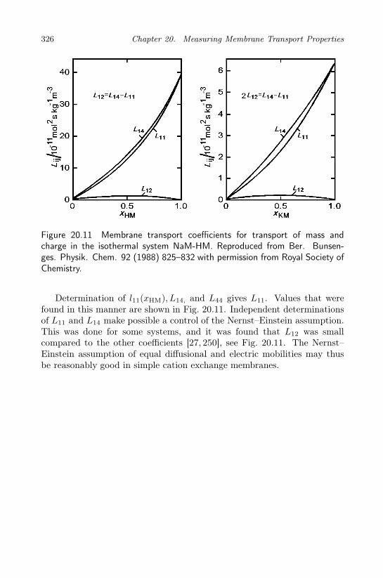
326 Chapter 20. Measuring Membrane Transport Properties
Figure 20.11 Membrane transport coefficients for transport of mass andcharge in the isothermal system NaM-HM. Reproduced from Ber. Bunsen-ges. Physik. Chem. 92 (1988) 825–832 with permission from Royal Society ofChemistry.
Determination of l11(xHM), L14, and L44 gives L11. Values that werefound in this manner are shown in Fig. 20.11. Independent determinationsof L11 and L14 make possible a control of the Nernst–Einstein assumption.This was done for some systems, and it was found that L12 was smallcompared to the other coefficients [27, 250], see Fig. 20.11. The Nernst–Einstein assumption of equal diffusional and electric mobilities may thusbe reasonably good in simple cation exchange membranes.

Chapter 21
The Impedance of an
Electrode Surface
We derive the impedance of an electrode surface. The surface is part of aheterogeneous system, the polymer electrolyte fuel cell. We introduce thechemical potential of the surface dipole, in order to be able to describe stor-age, depletion and redistribution of charges in the surface. An equivalentcircuit is predicted and compared with experimental results.
The impedance of an electrochemical cell is defined as minus the ratioof the applied oscillating potential difference, ∆φ, and the resulting electriccurrent density, jtot, that is produced in the outer circuit [266]:
Zcell ≡ −∆φ(ω)
jtot(ω)(21.1)
Measurements of ∆φ and jtot can be done with high precision as a functionof frequency ω, see e.g. Macdonald [267]. With two identical electrodesavailable, we measure the impedance of the path of charge transfer in twoelectrode materials (Za), two electrode surfaces (Zs) and in the electrolyte(Ze) between these:
Zcell = 2Za + 2Zs + Ze (21.2)
Frequently, Za is negligible. The variation in Zs with ω can be used toinvestigate rate limiting processes at the electrode surface. Spectra arenormally illustrated as Nyquist plots of Zcell according to
Zcell = ReZcell + i ImZcell (21.3)
where the imaginary part of the impedance is plotted as a function of thereal part. One example of such plots are shown in Fig. 21.1. The electrolyte
327
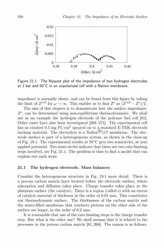
328 Chapter 21. The Impedance of an Electrode Surface
-0.02
-0.015
-0.01
-0.005
0 0.38 0.39 0.4 0.41 0.42
Z(I
m)
/ c
m2
Z(Re) / cm2
Figure 21.1 The Nyquist plot of the impedance of two hydrogen electrodesat 1 bar and 50C in an unpolarized cell with a Nation membrane.
impedance is normally ohmic, and can be found from this figure by takingthe limit of Zcell for ω → ∞. This enables us to find Zs as (Zcell − Ze)/2.
The aim of this chapter is to demonstrate how the surface impedance,Zs, can be determined using non-equilibrium thermodynamics. We shalluse as an example the hydrogen electrode of the polymer fuel cell [81].Other cases have also been investigated [268–271]. The experimental cellhas as catalyst 0.5 mg Pt/cm2 sprayed on to a standard E-TEK electrodebacking material. The electrolyte is a Nafion R©117 membrane. The elec-trode surface is part of a heterogeneous system, as shown in the close-upof Fig. 19.1. The experimental results at 50C give two semicircles, at zeroapplied potential. Two semi-circles indicate that there are two rate-limitingsteps involved, see Fig. 21.1. The problem is thus to find a model that canexplain two such steps.
21.1 The hydrogen electrode. Mass balances
Consider the heterogeneous structure in Fig. 19.1 more detail. There isa porous carbon matrix layer located before the electrode surface, whereadsorption and diffusion takes place. Charge transfer takes place at theplatinum surface (the catalyst). There is a region (called s) with an excessof catalyst material of thickness in the order of 0.01 mm. This constitutesour thermodynamic surface. The thicknesses of the carbon matrix andthe water-filled membrane that conducts protons on the other side of thesurface are larger, in the order of 0.2 mm.
It is reasonable that one of the rate-limiting steps is the charge transferstep. But what is the other one? We shall assume that it is related to theprocesses in the porous carbon matrix [81, 268]. The reason is as follows.

21.1. The hydrogen electrode. Mass balances 329
Only a small fraction of the platinum metal has an interface with the gasin the pores. This means that only a few active sites are accessible directlyfrom the gas. In order to reach most of the active sites on the Pt surface,hydrogen molecules must first adsorb to one of the surfaces involved (thegas-carbon, the gas-membrane or the gas-Pt surface), and then move to therest of the Pt surface by diffusion along the mentioned surfaces. They arriveat the active sites after passing some three phase contact lines (cf. Chap-ter 6). Hydrogen molecules cannot go directly to the contact line from thegas phase. This would lead to an infinite velocity of the gas close to thecontact line, which is impossible, see Remark 6.2. Early adsorption on asurface is therefore crucial for the hydrogen to reach most of the activesites on the Pt. Therefore, as the area of the Pt surface that is accessible tothe gas is only a fraction of the porous carbon surface, we assume that theabsorption/desorption on the walls of the pores is rate-limiting. We have(per mole of electrons produced)
1
2H2(g) → 1
2H2(a) (21.4)
The gas diffuses along the pore surface to the platinum catalyst in the x-direction. During diffusion some molecules desorb to form hydrogen in thegas phase again, so the adsorption has first order reaction kinetics in bothdirections:
r(x, t) =1
2kaH2cgH2
− 1
2kdH2caH2
(x, t) (21.5)
We use a course-grained description, in which all concentrations are given inmol/m3. The concentration cgH2
is then the gas concentration in the porestimes the porosity of the carbon layer. The course-grained concentrationcaH2
, is the surface excess concentration in mol/m2 times the surface area ofthe pores per unit of volume in m−1, and ka
H2and kd
H2are rate constants.
The reaction1
2H2(a) → H(s) (21.6)
takes place at the platinum surface. The charge transfer step follows. Thehydrogen atom dissociates on active sites of the platinum into protons inthe membrane and electrons in the electronically conducting carbon matrix:
H(s) → H+(m) + e−(a) (21.7)
Water is present in the carbon matrix and the membrane, but we neglectany role of water for this reaction here.
Each excess proton near the metal surface forms a dipole with an excesselectron in the metal surface. The surface thus has a dipole layer. The

330 Chapter 21. The Impedance of an Electrode Surface
Figure 21.2 Dipoles at an unpolarized and a polarized surface. One dipole ismade up by an ion and its image charge(s). This defines the surface polarizationPs or the surface double layer. The dipoles have a preferred direction in anelectric field.
surface thickness is such that the excess adsorptions (in mol/m2) of protons,ΓH+ , and of electrons, Γe− are equal. The dipole adsorption is
Γp(t) ≡ ΓH+(t) (21.8)
A schematic illustration of the dipoles in the surface is given in Fig. 21.2.In an unpolarized surface, the dipoles have a random direction. In anelectric field, the dipoles will orient themselves preferably in the directionof the field. The amount of dipoles in the surface depends probably onthe surface polarization, i.e. the applied electric potential or the electriccurrent density.
The charge transfer reaction increases the number of dipoles in the sur-face while the electric current j decreases it, giving
d
dtΓp = rsct −
j
F(21.9)
where rsct refers to the rate of the charge transfer reaction, and F is Fara-day’s constant. The surface polarization in the direction normal to thesurface is equal to the dipole concentration times Faraday’s constant, timesthe average distance, ds, between the charges
P s = dsFΓp (21.10)

21.2. The oscillating field 331
With constant ds, it follows that the surface polarization and the adsorptionof dipoles depend on each other. By eliminating Γp from Eq. (21.9), weobtain
rsct =1
F
(j +
1
ds
dP s
dt
)(21.11)
The surface polarization divided by the surface thickness gives the surfacepotential difference times the capacitance of the dipole layer, cp,
P s
ds= FΓp = csp∆sφ (21.12)
The polarization P s of Eqs. (21.10) and (21.12), is the polarization of thedouble layer and csp in Eq. (21.12) is the capacitance of the double layer.
21.2 The oscillating field
Consider the potential difference between the anode and the centre of themembrane (i.e. half the cell potential) in the oscillating field in the presenceof a direct current. The contributions from the dc and ac currents aresuperimposed:
∆φ = ∆φdc + ∆φac exp(iωt) (21.13)
The contribution to the emf of the two hydrogen electrodes are equal andopposite, and in the total cell potential they cancel each other. Each con-tribution is then the sum of the potential difference across one surface andhalf the membrane:
∆φdc = ∆sφdc +1
2∆mφdc and ∆φac = ∆sφac +
1
2∆mφac (21.14)
The electric current similarly has direct (dc) and alternating (ac) currentcontributions
j = jdc + jac exp(iωt) (21.15)
In the membrane, which conducts by protons, one has
∆mφdc = rmjdc and ∆mφac = rmjac (21.16)
We want to find the potential differences across the surface.The surface polarization can also be written as the sum of a stationary
and an oscillating contribution
P s = P sdc + P s
ac exp(iωt) (21.17)
For the dc and the ac contributions to rsct this gives, using Eq. (21.11),
rsct,dc =1
Fjdc and rsct,ac =
1
F
(jac +
iωP sac
ds
)(21.18)

332 Chapter 21. The Impedance of an Electrode Surface
21.3 Reaction Gibbs energies
The reaction Gibbs energy of the adsorption is:
∆rGsad(x, t) =
1
2
(µa
H2(x, t) − µg
H2
)(21.19)
We assume equilibrium between the chemical potential of adsorbed hydro-gen just before the surface and of atoms in the platinum surface, giving2µs
H = µaH2
(x = 0), where x = 0 is the position of the surface. The hydro-gen gas in the experiment has a constant (position and time independent)pressure, leading to a constant µg
H2. The anode is located at x < 0 and the
membrane at x > 0. In the coarse-grained description, transport takes placealong a coordinate normal to the surface of the membrane. All variablesare then independent of coordinates parallel to the surface.
The change in Gibbs energy at the surface due to the neutral species is:
∆nGsct(t) ≡ −1
2µa
H2(x = 0, t) (21.20)
For the total electrode reaction, we obtain
∆nGs = ∆rG
sad(x = 0, t) + ∆nG
sct(t) = −1
2µg
H2(21.21)
21.4 The electrode surface impedance
We describe the consecutive steps. We consider the electrode backing tobe continuous along the x-axis, while the electrode interfaces are describedas a Gibbs surface starting at position 0. Processes in the membrane areneglected.
21.4.1 The adsorption-diffusion layer in front of the catalyst
The time-dependence of the concentration of hydrogen at position x in theanode is given by
∂caH2(x, t)
∂t= −
∂JaH2
(x, t)
∂x+
1
2kaH2cgH2
− 1
2kdH2caH2
(x, t) (21.22)
where
JaH2
(x, t) = −DaH2
∂caH2(x, t)
∂x(21.23)
is the coarse-grained diffusion flux (in mol/m2s) of molecular hydrogenalong the surface of the pores in the carbon matrix to the catalyst surface
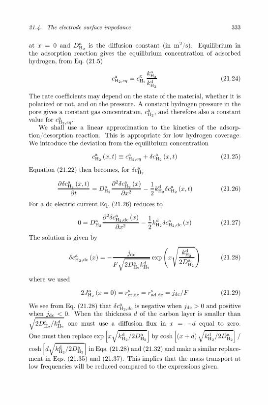
21.4. The electrode surface impedance 333
at x = 0 and DaH2
is the diffusion constant (in m2/s). Equilibrium inthe adsorption reaction gives the equilibrium concentration of adsorbedhydrogen, from Eq. (21.5)
caH2,eq = cgH2
kaH2
kdH2
(21.24)
The rate coefficients may depend on the state of the material, whether it ispolarized or not, and on the pressure. A constant hydrogen pressure in thepore gives a constant gas concentration, caH2
, and therefore also a constantvalue for caH2,eq.
We shall use a linear approximation to the kinetics of the adsorp-tion/desorption reaction. This is appropriate for low hydrogen coverage.We introduce the deviation from the equilibrium concentration
caH2(x, t) ≡ caH2,eq + δcaH2
(x, t) (21.25)
Equation (21.22) then becomes, for δcaH2
∂δcaH2(x, t)
∂t= Da
H2
∂2δcaH2(x)
∂x2− 1
2kdH2δcaH2
(x, t) (21.26)
For a dc electric current Eq. (21.26) reduces to
0 = DaH2
∂2δcaH2,dc (x)
∂x2− 1
2kdH2δcaH2,dc (x) (21.27)
The solution is given by
δcaH2,dc (x) = − jdc
F√
2DaH2kdH2
exp
(x
√kdH2
2DaH2
)(21.28)
where we used
2JaH2
(x = 0) = rsct,dc = rsad,dc = jdc/F (21.29)
We see from Eq. (21.28) that δcaH2,dc is negative when jdc > 0 and positivewhen jdc < 0. When the thickness d of the carbon layer is smaller than√
2DaH2/kd
H2one must use a diffusion flux in x = −d equal to zero.
One must then replace exp[x√kdH2/2Da
H2
]by cosh
[(x+ d)
√kdH2/2Da
H2
]/
cosh[d√kdH2/2Da
H2
]in Eqs. (21.28) and (21.32) and make a similar replace-
ment in Eqs. (21.35) and (21.37). This implies that the mass transport atlow frequencies will be reduced compared to the expressions given.

334 Chapter 21. The Impedance of an Electrode Surface
We use
µaH2
(x, t) = µa,0H2
+RT ln
(caH2
(x, t)
ca,0H2
)
= µa,0H2
+RT ln
(caH2,eq
ca,0H2
)+RT ln
(caH2
(x, t)
caH2,eq
)
= µaH2,eq +RT ln
(caH2
(x, t)
caH2,eq
)(21.30)
for the chemical potential of hydrogen, where µ a,0H2
and ca,0H2are standard
values. To linear order in δcaH, this gives
µaH2
(x, t) = µaH2,eq +RT ln
(1 +
δcaH2(x, t)
caH2,eq
)= µa
H2,eq +RTδcaH2
(x, t)
caH2,eq
(21.31)By introducing Eq. (21.28), we obtain
µaH2,dc (x) = µa
H2,eq −jdcRT
FcaH2,eq
√2Da
H2kdH2
exp
(x
√kdH2
2DaH2
)(21.32)
The Gibbs energy change over the whole layer becomes
∆rGad,dc = µsH,dc −
1
2µg
H2=
1
2
[µa
H2,dc (x = 0) − µaH2,dc (x = −∞)
]
= − jdcRT
2FcaH2,eq
√2Da
H2kdH2
(21.33)
∆rGad,dc gives a contribution to the surface potential drop viaδµa
H2,dc (x = 0).The ac contribution to caH2
(x, t) is also small. Equation (21.26) togetherwith Eq. (21.23) therefore reduce to
iωδcaH2,ac (x) = DaH2
∂2δcaH2,ac (x)
∂x2− 1
2kdH2δcaH2,ac (x) (21.34)
The solution to Eq. (21.34) becomes
δcaH2,ac(x) = −A exp
[x
√kdH2
2DaH2
(1 + iωτad)
](21.35)

21.4. The electrode surface impedance 335
where the relaxation time of the adsorption is
τad =2
kdH2
=2caH2,eq
kaH2cgH2
(21.36)
We used Eq. (21.24) in the last equality. The constant A in Eq. (21.35)must be determined from the boundary condition in x = 0. The resultingcontribution to the chemical potential, cf. Eq. (21.31), due to the ac currentis
µaH2,ac (x) = RTδcaH2,ac (x) /caH2,eq
= − ART
caH2,eq
exp
[x
√kdH2
2DaH2
(1 + iωτad)
](21.37)
The contribution due to a small dc current has already been given as thesecond term on the right hand side of Eq. (21.32).
The total amount of adsorbed hydrogen molecules on the pore surfacedue to the ac current, is
naH2,ac =
∫ 0
−∞
δcaH2,ac (x) dx = −A√
2DaH2
kdH2
(1 + iωτad)(21.38)
The ac contribution to the reaction rate for the adsorption reaction is thengiven by
rsad,ac = −kdH2
∫ 0
−∞
δcaH2,ac (x) dx = −kdH2n a
H2,ac = A
√2Da
H2kdH2
1 + iωτad(21.39)
The corresponding reaction rate for the charge transfer reaction is given by
rsct,ac = 2JaH2
(x = 0) = A√
2DaH2kdH2
(1 + iωτad) = (1 + iωτ ad)rs,aad,ac
(21.40)
The ac contribution to the reaction Gibbs energy of the adsorption is
∆rGad,ac =1
2(µa
H2,ac(x = 0) − µgH2,ac
) =1
2µa
H2,ac (x = 0) = − ART
2caH2,eq
(21.41)
where we used Eq. (21.37). By eliminating A in Eq. (21.41) usingEq. (21.40) we find,
∆rGad,ac = −ZadF2rsct,ac (21.42)
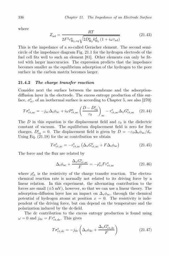
336 Chapter 21. The Impedance of an Electrode Surface
where
Zad =RT
2F 2caH2,eq
√2Da
H2kdH2
(1 + iωτad)(21.43)
This is the impedance of a so-called Gerischer element. The second semi-circle of the impedance diagram Fig. 21.1 for the hydrogen electrode of thefuel cell fits well to such an element [81]. Other elements can only be fit-ted with larger inaccuracies. The expression predicts that the impedancebecomes smaller as the equilibrium adsorption of the hydrogen to the poresurface in the carbon matrix becomes larger.
21.4.2 The charge transfer reaction
Consider next the surface between the membrane and the adsorption-diffusion layer in the electrode. The excess entropy production of this sur-face, σs
ct, of an isothermal surface is according to Chapter 5, see also [270]:
Tσsct,ac = −jac∆sφac + iωP s
ct,ac
(D −Ds
eq
ε0
)
ac
− rsct,ac∆nGsct,ac (21.44)
The D in this equation is the displacement field and ε0 is the dielectricconstant of vacuum. The equilibrium displacement field is zero for freecharges, Ds
eq = 0. The displacement field is given by D = −ε0∆sφac/ds.Using Eq. (21.18) for the ac contribution we obtain
Tσsct,ac = −rsct,ac
(∆nG
sct,ac + F∆sφac
)(21.45)
The force and the flux are related by
∆sφac +∆nG
sct,ac
F= −ρs
ctFrsct,ac (21.46)
where ρsct is the resistivity of the charge transfer reaction. The electro-
chemical reaction rate is normally not related to its driving force by alinear relation. In this experiment, the alternating contribution to theforces are small (±5 mV), however, so that we can use a linear theory. Theadsorption-diffusion layer has an impact on ∆sφac, through the chemicalpotential of hydrogen atoms at position x = 0. The resistivity is inde-pendent of the driving force, but can depend on the temperature and thepolarization induced by the dc-field.
The dc contribution to the excess entropy production is found usingω = 0 and jdc = Frsct,dc. This gives
Tσsct,dc = −jdc
(∆sφdc +
∆nGsct,dc
F
)(21.47)

21.4. The electrode surface impedance 337
For small dc-currents the linear law is thus:
∆sφdc +∆nG
sct,dc
F= −ρs
ctFrsct,dc = −ρs
ctjdc (21.48)
which is exactly the same relation as for the ac current, Eq. (21.46).
21.4.3 The impedance spectrum
The impedance spectrum in Fig. 21.1 is the sum of contributions from eachlayer, cf. Eq. (21.2). The surface impedance can be defined as
Zs ≡ −∆sφac
jac(21.49)
We can now find the surface impedance by adding Eqs. (21.42) and (21.46).This gives
∆sφac +∆nG
sac
F= ∆sφac = − (ρs
ct + Zad)Frsct,ac (21.50)
using a constant chemical potential of the hydrogen gas, cf. Eq. (21.21).Furthermore, it follows from Eqs. (21.11) and (21.12) that
Frsct,ac = jac + iωcsp∆sφac (21.51)
By combining Eqs. (21.49)–(21.51), we obtain the surface impedance
Zs =ρsct + Zad
1 + iωcsp (ρsct + Zad)
(21.52)
When ω → ∞, we see thatZs
ω→∞ = 0 (21.53)
In this case, the measurement gives the ohmic resistance of the cell.The limiting behavior ω → 0 gives
Zsω→0 = Zω→0,ad + ρs
ct (21.54)
The expression for Zad can be abbreviated by:
Zad =1
Y0
√τ−1ad + iω
(21.55)
with the relaxation time, τad = 2/kdH2
, see Eq. (21.36), and the admittance:
Y0 =4F 2
RTcaH2,eq
√Da
H2(21.56)

338 Chapter 21. The Impedance of an Electrode Surface
The relaxation time is constant, while the admittance is proportional tothe concentration of hydrogen in the gas phase.
In practice there may be non-ideal contributions to the impedance ofthe surface. A constant phase element (CPE) has been used, rather thana capacitance in parallel with the resistance, to compensate for surfaceheterogeneities. The CPE is defined by:
ZCPE =1
Tct(iω)αct(21.57)
The phase angle of the CPE is constant and independent of the frequency.When αct=1, Tct= csp. The more depressed the semi-circle is, the lower isthe value of α. The corresponding relaxation time is:
τct = (Tctρct)1/αct (21.58)
The experimental results below support, with the modification Eq. (21.58),the theoretical model.
21.5 A test of the model
The theoretical expression (21.56) predicted a pressure variation in theadmittance, Y0. The impedance of the cell was therefore measured at fivepressures between 1 and 4 bar, and at constant temperature (50oC). Theapplied dc potential was also varied. The impedance was found sweepingover a frequency range from 10 kHz to 10 mHz. An amplitude of 5 mV wasused. Figure 21.1 gives results for zero applied potentials at 1 bar.
The high frequency intercept with the real axis in Fig. 21.1 was constantin all spectra recorded, it was 0.39 ± 0.01 Ω cm2. This value, which is theresistance of the Nafion R©117 membrane in the cell, is in good agreementwith results reported in the literature for this temperature [268].
The high frequency regime of the impedance diagram, is according tothe previous section, Eqs. (21.52) and (21.57), related to the charge transferstep. The peak is not a perfect semicircle, which is possibly caused bythe heterogeneity of the electrode surface. The relaxation time of thisphenomenon depends on the applied potential (not shown), which is likelyfor a charge transfer step. The relaxation times for the two steps are given inTable 21.1 as a function of hydrogen pressure, for an unpolarized electrode.
The low frequency semicircle was fitted to the Gerischer phase element.The relaxation time τad did not vary with the applied dc potential, aspredicted from Eq. (21.36). The admittance varied linearly with caH2,eq, aspredicted from Eq. (21.56) and shown in Fig. 21.3. The slope of Fig. 21.3

21.6. The reaction overpotential 339
Table 21.1 Relaxation times as a function of hydrogen pressure.
pH2/bar τct/s τad/s
1 2.9 62.26 5.5 63.06 6.5 64.00 6.9 6
50
100
150
200
250
10 20 30 40 50 60
Y0
(104 s
1/2 /
m2 )
caH2, eq (mol/m3)
Figure 21.3 The admittance Y0 of the hydrogen electrode of the polymerelectrolyte fuel cell plotted as a function of hydrogen pressure. Reproducedfrom J. Membr. Sci. 282 (2006) 96–108 with permission of Elsevier.
was used to find a diffusion coefficient, DaH2
=1×10⁻⁷ m2/s [268], assumingkaH2
= kdH2
.Lower temperatures have revealed a shoulder in the impedance diagram.
This means that the model described above is not complete, but mustbe refined, probably by including a rate-limiting role for the hydration ofprotons, see [268,272–274].
21.6 The reaction overpotential
When impedance experiments are done in the presence of a constant appliedpotential, the total potential is a sum of a constant part and an oscillatingpart:
∆φtot(t) = ∆φdc + ∆φ(ω) (21.59)

340 Chapter 21. The Impedance of an Electrode Surface
We can deal with the two parts separately. The constant part of the poten-tial produces a constant (dc) current that determines the state of surfacepolarization. This state can be regarded as stationary. The balance equa-tion for dipoles then gives j/F = rs = jdc/F , and the entropy productionreduces to
Tσs = −jdc
(∆φ+
∆nGs
F
)(21.60)
The parenthesis is the effective driving force for the chemical reaction. Theelectrochemical reaction is frequently an activated process and the net driv-ing force can be substantial at the cathode of the fuel cell (cf. Chapter 19).The current density is a linear function of the driving force, only when theforce is small. When the driving force is large, the relationship becomesnonlinear, see e.g. [97].
The overpotential of a polarizable electrode is measured under steadystate conditions with the help of three electrodes. A net current is passedbetween the working electrode (the electrode of interest) and an auxiliaryelectrode. The electric potential drop across the surface for the given cur-rent density is ∆φ(jdc). The open circuit potential between the workingelectrode and a reference electrode is ∆φj→0. The overpotential is found asthe difference between ∆φ(jdc) and ∆φj→0:
η = ∆φ(jdc) − ∆φj→0 (21.61)
The measurement gives the overpotential as a function of current density.The non-linear relation is the so-called Butler–Volmer relation. The relationbetween η and jdc is complicated because the dipole adsorption dependson the state of the electrode, here represented by P s. Rubi and Kjelstrupshowed how this relation can be derived using non-equilibrium thermody-namics on the mesoscopic level [51].

Chapter 22
Non-Equilibrium Molecular
Dynamics Simulations
We describe a computer simulation technique that is designed to study trans-port processes. The name of the method is non-equilibrium molecular dy-namics simulations (NEMD). We shall describe how we can find transportcoefficients in one-phase fluids and heterogeneous systems from NEMD.Molecular explanations of the coefficients values are of interest. In a systemthat transports heat and mass, we can use NEMD to verify the assumptionof local equilibrium and of Onsager reciprocal relations. We examine alsothe linear nature of the flux-force relations.
Non-equilibrium molecular dynamics simulations (NEMD) is a com-puter technique that is designed to investigate particle behavior in sys-tems with gradients in intensive variables. The system behavior followsfrom the interaction between the particles. Such interactions can for in-stance be described by a pair potential like the Lennard-Jones potential[275, 276].
Algorithms that characterize NEMD were developed by Hafskjold andcoworkers [277]. Gradients are applied to the system by perturbation of itsboundaries, in so-called boundary driven NEMD. Alternatively, one can setup a flux via the boundaries, and study resulting gradients. The methodsimulates therefore experiments in its determination of transport properties.We present the useful technique here, drawing especially on the work of Haf-skjold and coworkers [65,66,149,277–283] and others [284–288]. In additionto presenting the technique, we present some results [39,40,65,67,112,289]that confirm the basic assumptions in classical non-equilibrium thermody-namics. We will not discuss the use of the Kubo relations (see Fig. 1.2)to determine transport coefficients using equilibrium molecular dynamicssimulations from integrals over equilibrium flux-flux correlation functions.
341

342 Chapter 22. Non-Equilibrium Molecular Dynamics Simulations
Figure 22.1 A typical trajectory for one particle in a gas (only one particleis shown). The particle moves according to Newton’s laws and interacts witha Lennard-Jones potential. The distance between the points is one time-stepin the calculation. The length of the mean free path is shown by the bar.(Courtesy of B. Hafskjold)
In NEMD, the computer is used to solve Newton’s equations of motionfor the particles in the system. On a microscopic level, the particle motionappears chaotic, even if Newton’s laws are reversible in time. A typicaltrajectory for one particle in a system in equilibrium is given in Fig. 22.1.Many particles are moved around in the box, but only one trajectory isshown. Whenever this trajectory changes, a collision takes place. Theparticles collide with each other and with the walls. All thermodynamicand transport properties of the system are derived from the mechanicalproperties of the set of colliding particles in NEMD.
After 4000 time steps of calculation, the particles in each layer alreadyhave a molecular velocity distribution equal to a Maxwell distribution. Ithas also been verified that the temperature, as calculated from the equipar-tition principle, is the same in all three directions in space, in a homogeneoussystem as well as a heterogeneous one. Figure 22.2 shows the temperature ina volume element in the center of a system with two types of particles. Wesee the fluctuations in the dimensionless temperature, T ∗ = kBT/ε, whereε is the potential depth of the Lennard-Jones type potential of the heavyparticles and kB is Boltzmann’s constant. The technique uses dimensionlessvariables, which are further explained in Table 22.1. The fluctuations inFig. 22.2 obeyed δT/T < 0.03 [65].

Chapter 22. Non-Equilibrium Molecular Dynamics Simulations 343
Figure 22.2 Fluctuations in dimensionless temperature at some position inthe box during stationary state heat conductance in a two-component mixture.The system is the same as in Fig. 22.6 (Courtesy of B. Hafskjold).
NEMD and other computer techniques utilize periodic boundary con-ditions, in order to obtain a larger and more representative system in acomputer-efficient manner. Instead of finding the average over one largesystem, one finds the average over many small identical systems. A parti-cle leaving one box enters the next in a way that makes the system periodic,and introduces a plane of symmetry in the center of each box. NEMD sim-ulations are often run until a stationary state is obtained. An average overa layer with only a few particles, but over long time intervals, can then re-place an average over many particles (the ergodic hypothesis). The averagebehavior of all particles is taken as the collective behavior of the ensemblein a layer.
NEMD simulations can be used to study properties of ensembles ofparticles, in both global equilibrium and out of global equilibrium. In globalequilibrium, all boundaries are set with the same conditions; out of globalequilibrium they are not. In order to determine transport properties, oneoften requires also the equilibrium properties of the system. It is therefore ofinterest to use NEMD to find both types of data. Variations of variables likethe particle density, the temperature and the pressure, in the homogeneous

344 Chapter 22. Non-Equilibrium Molecular Dynamics Simulations
1−4 61−68 125−128
TT
TH
H
L
Figure 22.3 The box in a NEMD simulation is divided into a number ofequal layers (128 in this case). Boundary conditions, indicated here by thetemperatures TL and TH, are symmetric around the center of the box.
phases, and across the interface between a liquid and its vapor, are ofinterest. One can use this information to first find the equation of state (inequilibrium systems), and then the transport properties (in non-equilibriumsystems).
Simulations cannot be expected to give values found by experiments,even if much progress has been made in this direction the last few years[290]. The expression for the interaction potential is a guess for a realsystem. The advantage of NEMD is that trends and variations in propertiescan be traced back to part(s) of the interaction potential that causes thevariation. This property means that NEMD gives molecular insight insystem behavior. It becomes possible to distinguish between importantand minor effects. This is important when it is necessary to introduceassumptions. This is the usefulness of NEMD: it acts as a tool to helpunderstand experimental results, and it can be used to test assumptionsmade in the theory. Since it is difficult to do experiments in heterogeneoussystems, the technique is very valuable.
We continue to describe details of the NEMD technique before wepresent results that confirm the hypothesis of local equilibrium and of theOnsager relations, in a one-phase system, and at a surface.
22.1 The system
The NEMD simulation starts with construction of a rectangular box withdimensions Lx, Ly and Lz. Here x is the direction along the box, y isthe vertical direction and z is the depth direction, see Fig. 22.3. The boxcontains N particles. The density is changed by varying the box size, using:
ρ = VNA
N= LxLyLz
NA
N(22.1)
where NA is Avogadro’s number and ρ is the overall molar density of parti-cles. We are interested in transports in the x−direction. In this direction,

22.1. The system 345
the box is divided into equal layers for monitoring of local properties. Thecell used is usually not cubic Lx > Ly = Lz. The temperature, density,pressure, composition, enthalpy, fluxes, and other properties of interest canbe computed in each layer. The box in Fig. 22.3 has, say, a temperaturegradient between the ends and the center of the box. All the stationarystate simulations were done such that profiles (fluxes) are symmetric (anti-symmetric) with respect to the center of the box in the x-direction. Periodicboundary conditions are used. When a particle crosses one of the bound-ary planes it is reinserted with the same velocity on the opposite side ofthe box.
Irreversibilities are introduced by controlling some variables in layers inthe middle or near the ends of the box (in the x-direction). The walls of thebox can either be directly interacting walls, like in a porous system [288], orregions where the temperature, chemical potential, or momentum is set bya local perturbation of the system [284]. A gradient in chemical potentialor a concentration gradient can be introduced by manipulating the particletypes and molecular properties in the end and center regions, for instance,by particle swapping [291–293].
In the simulations of a homogeneous mixture we used N = 512 withequal numbers of each component and Lx = 2Ly = 2Lz [65]. The boxwas divided into 32 layers in the x-direction. In order to give the systema certain temperature profile, layers 1 and 32 at the end of the box werethermostatted to a high temperature TH and layers 16 and 17 in the centerof the box were thermostatted to a low temperature TL. The amounts ofenergy added and removed are equal, so that total energy is conserved andthe energy flux is constant. A diffusion flux was simulated by swappingparticles of different types between the layers in the center and the layersat the end of the cell. The velocities of these particles were scaled so thatno kinetic energy was exchanged and total momentum was conserved.
In the simulations of a one component two-phase system, N = 4096was used with Lx = 16Ly = 16Lz [39, 40]. The box was divided into128 layers in the x-direction. Layers 1–4 and 125–128 were thermostattedto a high temperature while layers 61–64 and 65–68 were thermostattedto a low temperature, see Fig. 22.4. A mass flux from the vapor to theliquid (condensation) was simulated by removing particles from the lowtemperature layers in the center, layers 61–68, moving them to one of thehigh temperature layers at the ends of the cell. In this process, the particlemaintains its y- and z-coordinates, while its x-coordinate is changed by±Lx/2.
When a non-equilibrium system is in a stationary state, the fluxes ofenergy and mass are constant. A liquid and a vapor phase may coexistin this case, when the boundary conditions are appropriate. The liquid

346 Chapter 22. Non-Equilibrium Molecular Dynamics Simulations
Cold layers
61− 68
Hot layers
1− 4Hot layers
125−128
Figure 22.4 Lennard-Jones spline particles distributed in a temperature gra-dient that leads to phase separation. The cell is symmetric, with hot ends anda cold center.
phase appears in the middle of the box, since energy is removed there. Oneach high-temperature side, a vapor phase is formed. Two surfaces arethen formed between the vapor and liquid without disturbances from theboundaries of the box. The situation is thus ideal for studies of the surface.A snapshot of the situation is illustrated in Fig. 22.4.
22.1.1 The interaction potential
Between every pair of particles, a potential exists, so that particles closeto each other repel and particles farther away from each other attract eachother. A common pair potential for particle interaction in fluids is theLennard-Jones pair potential, or simply the Lennard-Jones potential:
uij = 4ǫij
[(σij
rij
)12
−(σij
rij
)6]
(22.2)
Here, uij is the potential between particle i and j, ǫij is the minimum ofthe potential between particle i and j, ri and rj are the positions of particlei and j, rij ≡ |ri − rj | is the distance between particle i and j, and σij isthe distance between particles when the potential is equal to zero. In aone component system, there is only one such distance σ and one minimumpotential ǫ. In a two component mixture, there are three different σ’s andthree different minimum potentials.
In the computations one usually uses a cut-off Lennard-Jones potential,which is taken to be equal to zero for distances beyond a cut-off distance,r > rc. One also uses a shifted cut-off Lennard-Jones potential, which istaken to be equal to the cut-off Lennard-Jones potential minus its valuein r = rc. The cut-off Lennard-Jones potential is often used in moleculardynamics simulations. This potential accelerates the particles when theymove across rc and changes the system’s energy. In order to avoid thiscontribution and obtain a consistent description of equilibrium as well asnon-equilibrium properties, it is necessary to shift the cut-off Lennard-Jones

22.2. Calculation techniques 347
potential. The Lennard-Jones spline potential, with the spline distancers = (26/7)
1/6σij , is given by:
uij = 4ǫij
[(σij
rij
)12
−(σij
rij
)6]
r ≤ rs
uij = αij (rij − rc)3
+ βij (rij − rc)2
rs ≤ r ≤ rc
rc =67
48rs ≃ 1.737σij
αij = −387072
61009
ǫijr3s
βij = −24192
3211
ǫijr2s
(22.3)
The potential obtained in this manner is a modified version of the Lennard-Jones potential. The two potentials are the same until the distance isrs. After that the spline potential continues until the cut-off distance,rc, by Eq. (22.3b)–(22.3e), while the Lennard-Jones potential continues byEq. (22.2). The spline potential is less long-ranged than the Lennard-Jonespotential. Plots of the two potentials are given in Fig. 22.5. The splinepotential was used to generate the picture in Fig. 22.4.
Lennard-Jones potentials do not deal with charged particles. In orderto deal with ionic or polarized systems, one normally adds a Coulomb typepotential or a Yukawa potential to the expressions above [66]. Chargedsystems are much less studied than electroneutral systems.
The NEMD program uses reduced variables instead of real variables.Examples of reduced variables are given in Table 22.1. Variables are madedimensionless by division by σij , mass, minimum interaction potential forcomponent 1. In this table, kB is the Boltzmann constant. The advantageof using reduced variables in NEMD is that they can be converted to anyfluid of interest. For instance, for argon-like particles ǫ/kB = 124 K, m =6.64× 10⁻²⁶ kg, and σ = 3.42× 10⁻¹⁰ m. When Lennard-Jones potentialsare used to model a mixture, each molecule is approximated by a sphere ofa given diameter σ and with a given interaction parameter ǫ.
22.2 Calculation techniques
In NEMD, all molecular properties are calculated from the mechanical prop-erties of the system. Some of these calculations are explained below for abox divided into 128 layers. The expressions for 32 layers can be obtainedby replacing 128 and 64 by 32 and 16 in the formulae below. The results are

348 Chapter 22. Non-Equilibrium Molecular Dynamics Simulations
Figure 22.5 The Lennard-Jones potential (solid line) and the Lennard-Jonesspline potential (stipled line) as a function of the dimensionless inverse distancebetween particles. The symbols ai and aj correspond to σij in the text.
mostly reported in reduced units, see Table 22.1, so that conversion into realvariables can be done as one prefers. Consider again the box in Fig. 22.3.For stationary states, the fluxes can be found using time averages in all 128layers. Likewise, we can calculate the average kinetic energies, potentialenergies and the number of particles in each layer. Using the symmetry ofthe system around the center of the box, the mean of the properties in eachhalf is calculated. In this way, the statistics become even better. The resultthen stems from a system with only 64 layers, where each layer is the meanof the corresponding two layers in the original system. The volume of sucha pair of layers is V/64, where V = LxLyLz is the volume of the box. Theparticle density of component k in a layer is the number of particles of thatcomponent, Nk,ν , in each pair of layers divided by the volume of the pairof layers:
ρk,ν ≡ Nk,ν64
V(22.4)
The molar flux, Jk,ν , and the average velocity, vk,ν , of component k in eachpair of layers ν, with ν = 1, . . . , 64, is found from:
Jk,ν ≡ ρk,νvk,ν
NA≡ 64
V NA
∑
i∈k,i∈layers
vi (22.5)
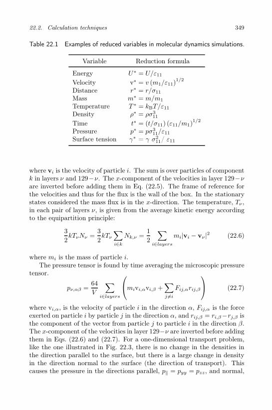
22.2. Calculation techniques 349
Table 22.1 Examples of reduced variables in molecular dynamics simulations.
Variable Reduction formula
Energy U∗ = U/ε11Velocity v∗ = v (m1/ε11)
1/2
Distance r∗ = r/σ11
Mass m∗ = m/m1
Temperature T ∗ = kBT/ε11Density ρ∗ = ρσ3
11
Time t∗ = (t/σ11) (ε11/m1)1/2
Pressure p∗ = pσ311/ε11
Surface tension γ∗ = γ σ211/ ε11
where vi is the velocity of particle i. The sum is over particles of componentk in layers ν and 129−ν. The x-component of the velocities in layer 129−νare inverted before adding them in Eq. (22.5). The frame of reference forthe velocities and thus for the flux is the wall of the box. In the stationarystates considered the mass flux is in the x-direction. The temperature, Tν ,in each pair of layers ν, is given from the average kinetic energy accordingto the equipartition principle:
3
2kTνNν =
3
2kTν
∑
i∈k
Nk,ν =1
2
∑
i∈layers
mi|vi − vν |2 (22.6)
where mi is the mass of particle i.The pressure tensor is found by time averaging the microscopic pressure
tensor.
pν,αβ =64
V
∑
i∈layers
mivi,αvi,β +
∑
j 6=i
Fij,αrij,β
(22.7)
where vi,α, is the velocity of particle i in the direction α, Fij,α is the forceexerted on particle i by particle j in the direction α, and rij,β = ri,β−rj,β isthe component of the vector from particle j to particle i in the direction β.The x-component of the velocities in layer 129−ν are inverted before addingthem in Eqs. (22.6) and (22.7). For a one-dimensional transport problem,like the one illustrated in Fig. 22.3, there is no change in the densities inthe direction parallel to the surface, but there is a large change in densityin the direction normal to the surface (the direction of transport). Thiscauses the pressure in the directions parallel, p‖ = pyy = pzz, and normal,

350 Chapter 22. Non-Equilibrium Molecular Dynamics Simulations
p⊥ = pxx, to the surface to be different in the interfacial region. The off-diagonal elements of the pressure tensor are found to be zero. The surfacetension is due to the difference between the parallel and the normal pressureand is calculated from
γ =Lx
128
64∑
ν=1
(p‖ − p⊥
)(22.8)
Todd et al. [294] developed an alternative algorithm for pressure calculationin heterogeneous systems; the method-of-planes. This gives the pressuretensor for planar surfaces [112].
The measurable heat flux in each layer, J′q,ν , cannot be computed di-
rectly, because it is not a mechanical property. It is, however, related tothe total heat flux (the energy flux), Jq,ν , by
J′q,ν = Jq,ν −
∑
i∈k
HkJk,ν (22.9)
where Hk is the partial molar enthalpy of component k. In order to de-termine the partial molar enthalpy, we need the enthalpy as a function ofcomposition, which in principle requires a series of simulations [280, 282].The total heat flux can be expressed in terms of mechanical quantities asfollows [276,295]:
Jq,ν =64
V
∑
i∈layers
[1
2miv
2i + φi
]vi +
1
2
∑
j 6=i
[vi · Fij ] rij
(22.10)
where φi is the potential energy of particle i in the field of all the otherparticles, Fij is the force acting on i due to j, and rij = ri − rj is thevector from the position of j to the position of i. The measurable heatflux can then be determined from Eq. (22.9). Three important cases avoidthe non-trivial task of determining Hk; (1) binary isotope mixtures withH1 = H2, giving J′
q,ν = Jq,ν in the mean molar reference frame, for whichJ1 = −J2, and (2) binary mixtures for which J1 = J2 = 0, again withJ′
q = Jq as the result, and (3) ideal mixtures with Hk equal to the molarenthalpy of component k. The energy flux is computed for each layer withEq. (22.10), except that the first summation includes only those particlesi that are in the given layer. The energy flux is then computed from theamount of energy added and withdrawn. When the system is not uniform,care must be taken in the computation of the measurable heat flux.
Transport coefficients can also be calculated from equilibrium systems,using the Kubo relations [296].

22.3. Verifying the assumption of local equilibrium 351
22.3 Verifying the assumption of local equilibrium
NEMD simulations were used by Hafskjold and coworkers [39, 65, 66, 111,112] to confirm the assumption of local equilibrium in systems where heatand mass were transported. A binary homogeneous mixture and a puretwo-phase system were studied. Both systems were subject to enormoustemperature gradients, of the order of magnitude 108 K/m. This temper-ature gradient, as well as the magnitude of the mass flows considered, aremostly beyond realization in a laboratory.
22.3.1 Local equilibrium in a homogeneous binary mixture
An equimolar binary isotope gas mixture of N = 512 particles in a rect-angular, closed box was studied in a temperature gradient [65, 149]. Theenthalpy, H, and the pressure, p, were calculated for each layer in thepresence and absence of the temperature gradient. For the same state
Figure 22.6 The enthalpy (circles), the potential energy (squares) and thepressure (triangles) in a two-component mixture in a temperature gradient(open symbols) and in mixtures that are in global equilibrium with the samestate variables (filled symbols). The particles interact with a Lennard-Jonesspline potential. They have the same diameter, the same potential depth, anda mass ratio of m1/m2 = 10. Reproduced from Stat. Phys. 78 (1995) 463–494with permission of Springer.

352 Chapter 22. Non-Equilibrium Molecular Dynamics Simulations
Figure 22.7 The dimensionless temperature gradient and the correspondinggradient in mole fraction for the system described in Fig. 22.6. (Courtesy ofB. Hafskjold)
variables, identical local values for H (circle symbols), p (triangular sym-bols) and potential energy U (square symbols) were obtained in the twocases [65]. The results are shown with open symbols in Fig. 22.6. Selectedresults for equilibrium calculations for the same state variables are shownwith filled symbols in the same figure. The results are the same, so it wasconcluded that thermodynamic relations are valid locally in the tempera-ture gradient. The extreme gradient across the volume element thus didnot lead to a violation of the assumption of local equilibrium. Hafskjoldand coworkers [282] reported that the assumption of local equilibrium wasalso true with a mass flux across the system. A surprisingly low numberof particles was enough to give a statistical basis for calculation of thermo-dynamic properties. This can be explained by the use of averages over asufficiently long time interval. On the average there were Nν =16 particlesin a volume element, and the fluctuation in Nν was δNν/Nν ≈ 0.3. Thisfluctuation in particle number is the cause of the temperature fluctuationseen in Fig. 22.2, but δT/T was only ≈ 0.03. A system in local equilibriumand a system in global equilibrium differ in the way they fluctuate [109]. Itwas also found that heavy particles concentrated in the cold parts of the boxwhile the light particles concentrated in the warm parts, see Fig. 22.7 [149].This is discussed further below.

22.3. Verifying the assumption of local equilibrium 353
22.3.2 Local equilibrium in a gas-liquid interface
We also studied the two-phase systems in a temperature gradient [39]. Thephase diagram of the system was first determined. It is given in reducedunits in Fig. 22.8. The relations between the pressure, temperature and thedensity were determined for the homogeneous phases; the vapor as well asin the liquid. For the surface, the relation between the surface tension andthe temperature was determined. The NEMD cell contained 4096 particlesin this case. This number ensures that there are enough particles in thevapor phase to obtain meaningful averages. In order to address the questionof whether one is in the vapor or in the surface it is important to choose theoverall molar density such that the vapor region is much thicker than themean free path of the particles in this region. The cell was non-cubic, withratios Lx/Ly = Lx/Lz = 16, where Li is the length of the cell in the i-thdirection. By choosing the proper overall particle density and temperatures,and using the phase diagram in Fig. 22.8, a temperature gradient was usedto generate a liquid region in the center of the cell with vapor on bothsides. The box was subdivided into 128 layers, with a thickness 3
√1/2ρ in
meters, where ρ = N/LxLyLz is the overall density in the box. The meanfree path (cf. Fig. 22.1) was calculated from the formula, ℓ = 1/(σ2ρνπ
√2),
from kinetic gas theory, where σ is the diameter of the particles and ν isone of the vapor layers. In the simulations the mean free path had valuesup to about 10 layer thicknesses close to the triple point.
A particle flux from the vapor to the liquid (condensation) was simu-lated, using the algorithm that removed a particle from the low temperaturelayers in the center and inserted it into one of the high temperature layersat the end of the cell. The particle maintained its y- and z-coordinateswhile its x-coordinate was changed by ±Lx/2. In order to avoid large per-turbations of the energy of the system, the particle insertion was done witha probability given by the Boltzmann factor. NEMD simulations were donefor a number of cases along the phase line where two phases coexist, witha heat flux present, and with or without a particle flux. A snapshot of thedensity profiles in the half of the cell is shown for two cases in Fig. 22.9.
Gibbs [62] defined the surface as a transition region with a finite thick-ness bounded by planes of similarly chosen points, cf. Sec. 3.3. The sim-ulation results illustrated in Fig. 22.9 show that we can identify two suchplanes, for instance, planes where on one side the equation of state for thefluid is still valid, while on the other side this is no longer the case. Theregion where the equation of state for the liquid or for the vapor are notvalid, is then the surface. By such choices, the surface was found to have athickness of about 10 layers, which is about 5 nm in real units, for densitiesaway from the critical point. Ten layers is about the mean free path in the

354 Chapter 22. Non-Equilibrium Molecular Dynamics Simulations
Figure 22.8 Phase diagram for the Lennard-Jones spline fluid. Reproducedfrom J. Colloid Interface Sci. 232 (2000) 178–185 with permission of Elsevier.
Figure 22.9 Density profiles from two NEMD simulations of heat and masstransfer through a surface. Case 1 is far from and Case 2 is close to the criticalpoint. Data are taken from Røsjorde et al. [39].

22.3. Verifying the assumption of local equilibrium 355
Figure 22.10 Temperature profiles from two NEMD simulations of heat andmass transfer through a surface, see also Fig. 22.9. Case 1 is far from andCase 2 is close to the critical point. Data are taken from Røsjorde et al. [39]
vapor close to the triple point. The thickness increased to about 25 layersclose to the critical point. The thickness, in particular, close to the triplepoint, is more than one would expect on the basis of a visual inspectionof the curves. Such a visual inspection can therefore not be used to deter-mine the surface position. The deviation from the equation of state for thehomogeneous phase already occurs before it shows up in the graph.
The temperature of the surface was calculated from the kinetic energiesof the particles within these boundaries. It was found to be in good ap-proximation equal to the temperature of the first liquid layer outside theclosed surface. The temperatures of all layers are plotted for the same casesof Fig. 22.9 in Fig. 22.10. For each layer, and for the closed surface, thetemperatures computed from velocity components along or normal to thesurface were the same. This serves as a first confirmation of the validity ofthe assumption of local equilibrium.
Finally, the surface tension from the NEMD simulations was plotted asa function of the temperature of the surface, see Fig. 22.11. For compari-son, the results of simulations for the equilibrium surface were also given.The figure shows that the surface is in local equilibrium in the presence oftemperature gradients of up to 3 × 10⁸ K/m between the cold and the hotlayers.

356 Chapter 22. Non-Equilibrium Molecular Dynamics Simulations
Figure 22.11 The surface tension as a function of the temperature of thesurface. The points in the curve derive from equilibrium (filled squares) andnon-equilibrium molecular dynamics simulations (open circles). Reproducedfrom J. Colloid Interface Sci. 299 (2006) 452–463 with permission of Elsevier.
Simon and coworkers [112] considered heat transfer in a box with 2000molecules of n-octane. The molecules interacted with a truncated Lennard-Jones potential, and had vibrational and rotational degrees of freedom.The equimolar surface was determined as mentioned above. Also, for thesesimulations, the surface tension for the stationary states was found to bethe same function of the surface temperature as in equilibrium. This againverified local equilibrium.
The value of the surface tension depends strongly on the cut-off of thepotential. If one wants to compare the predictions with experimental values,one should add tail corrections [297].
22.4 Verifications of the Onsager relations
Transport coefficients can be determined from NEMD simulations to testfor instance the Onsager relations. The coefficients are calculated, once theforces and their corresponding fluxes are computed.
22.4.1 A homogeneous binary mixture
Consider the binary mixture of isotopes that was studied by Hafskjold andKjelstrup Ratkje [65]. The barycentric frame of reference, see Sec. 4.4.1,

22.4. Verifications of the Onsager relations 357
was used, with J1 = −J2, and the following flux-force relations:
J ′q = lqq
(d
dx
1
T
)+ lqµ
[− 1
T
d(µT,1 − µT,2)
dx
]
J1 = lµq
(d
dx
1
T
)+ lµµ
[− 1
T
d(µT,1 − µT,2)
dx
] (22.11)
By calculating lqµ independent from lµq, Onsager relations can be tested.With a known heat flux and temperature difference across a (sub-)system,the stationary state thermal conductivity is given by:
λ = −(
J ′q
dT/dx
)
J1=0
=
(lqq −
lqµlµq
lµµ
)1
T 2(22.12)
The heat of transfer is
q∗ =
(J ′
q
J1
)
dT=0
=lqµ
lµµ(22.13)
Using Gibbs–Duhem’s equation, w1dµ1 +w2dµ2 = 0, the differential of thedifference of the chemical potentials at constant temperature and pressurecan be expressed by the weight fraction of the components, wi:
d (µT,1 − µT,2)
dx=
1
w2
∂µ1
∂w1
∂w1
∂x(22.14)
where we used w1 +w2 = 1. The thermal diffusion factor α can be definedas (see also Sec. 8.2):
αT = −(∂ ln(w1/w2)/∂x
∂lnT/∂x
)
J1=0
= − T
w1w2
(∂w1/∂x
∂T/∂x
)
J1=0
=lµq
lµµ
∂ lnw1
∂µ1
(22.15)The component flux can be expressed as
J1 = −ρw1D
(w2αT
d lnT
dx+
d
dxlnw1
)(22.16)
with the diffusion coefficient
D =lµµ
ρw2T
∂µ1
∂w1(22.17)
When the thermal conductivity, thermal diffusion factor, heat of transfer,and diffusion coefficient can be computed from NEMD results, Eqs. (22.12),
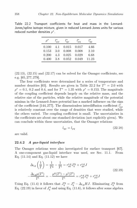
358 Chapter 22. Non-Equilibrium Molecular Dynamics Simulations
Table 22.2 Transport coefficients for heat and mass in the Lennard-Jones/spline isotope mixture, given in reduced Lennard-Jones units for variousreduced number densities ρ∗.
ρ∗ l∗µµ l∗qµ l∗µq l∗qq
0.100 4.1 0.015 0.017 4.660.153 3.0 0.008 0.008 2.100.200 4.3 0.025 0.029 6.680.400 3.8 0.052 0.049 11.23
(22.13), (22.15) and (22.17) can be solved for the Onsager coefficients, seee.g. [65, 277,279].
The four coefficients were determined for a series of temperature andnumber densities [65]. Results are given in Table 22.2 for T ∗ = 2.0 withρ∗ = 0.1, 0.2 and 0.4, and for T ∗ = 1.35 with ρ∗ = 0.153. The magnitudeof the coupling coefficient depends largely on the relative mass, and therelative size of the particles, while the relative magnitude of the potentialminima in the Lennard-Jones potential has a marked influence on the signof the coefficient [144,277]. The dimensionless interdiffusion coefficient l∗µµ
is relatively constant over the range of densities that were studied, whilethe others varied. The coupling coefficient is small. The uncertainties inthe coefficients are about one standard deviation (not explicitly given). Wecan conclude within these uncertainties, that the Onsager relations
lqµ = lµq (22.18)
are valid.
22.4.2 A gas-liquid interface
The Onsager relations were also investigated for surface transport [67].A one-component gas-liquid interface was used, see Sec. 11.1. FromEq. (11.14) and Eq. (11.12) we have
∆l,g
(1
T
)=
1
T g− 1
T l= rs,gqq J
′gq + rs,gqµJ
−∆l,gµ(T l)
T l= −µ
g(T l) − µl(T l)
T l= rs,gµq J
′gq + rs,gµµJ
(22.19)
Using Eq. (11.4) it follows that J ′gq = J ′l
q − ∆l,gHJ . Eliminating J ′gq from
Eq. (22.19) in favor of J ′lq and using Eq. (11.6), it follows after some algebra

22.5. Linearity of the flux-force relations 359
that
∆l,g
(1
T
)=
1
T g− 1
T l= rs,lqqJ
′lq + rs,lqµJ
−∆l,gµ(T g)
T g= −µ
g(T g) − µl(T g)
T g= rs,lµqJ
′lq + rs,lµµJ
(22.20)
In the calculations, it was documented that the Onsager relation
rs,gqµ = rs,gµq (22.21)
was valid. The coefficients for the liquid side are given by
rs,lqq = rs,gqq = rsqq
rs,lqµ = rs,lµq = rs,gµq − rs,gqq ∆l,gH
rs,lµµ = rs,gµµ − 2rs,gµq ∆l,gH + rs,gqq (∆l,gH)2
(22.22)
The results for the coupling coefficients are shown in Fig. 22.12. The On-sager relations, rs,gqµ = rs,gµq and rs,lqµ = rs,lµq , were valid within the numericalaccuracy of the calculation for gradients up to 109 K/m [67].
22.5 Linearity of the flux-force relations
One of the basic postulates of non-equilibrium thermodynamics is thatfluxes are linear combinations of all conjugate forces, see Eq. (7.12). Thispostulate can also be tested by NEMD [67]. The surface transfer coef-ficients, described in the previous subsection, were calculated using thelinear relations in Eqs. (22.19) and (22.20). There was no need to invokenon-linear terms in these calculations. The coefficients depended on thestate of the surface, here on the state variable γ, or equivalently, on thesurface temperature. The coefficients were thus not functions of the forcesor of the fluxes for temperature gradients investigated (up to 109 K/m).This is in accordance with the assumptions used in Sec. 7.2. Paolini etal. [298] found linear response for gradients up to 5.8 x 10¹⁰ K/m in aLennard-Jones fluid near the triple point. We do not consider systemswith a shear gradient in this book. For large shear gradients, non-linearcontributions to the heat flux were important [299,300].
22.6 Molecular mechanisms
NEMD offer insight in the transport mechanism. Simon and coworkers [112]determined the resistivity of the surface to heat transfer in a box with 2000

360 Chapter 22. Non-Equilibrium Molecular Dynamics Simulations
-14
-12
-10
-8
-6
-4
-2
0
2
1 2 3 4 5 6 7rsm
qa
nd
rsq
m/
10
-7m
2s m
ol-1
K-1
g / 10-3
N m-1
rs,g
mq, vapor side
rs,g
q m, vapor side
rs,l
mq, liquid side
rs,l
q m, liquid side
Figure 22.12 The coupling coefficient for evaporation and condensation ofone component, on the vapor side (top) and the liquid side (bottom). Coeffi-cients were obtained from NEMD simulations (points), and from kinetic theory(stipled lines). Reproduced from J. Colloid Interface Sci. 299 (2006) 452–463with permission of Elsevier.
molecules of n-octane. The molecules interacted with a truncated Lennard-Jones potential, and had vibrational and rotational degrees of freedom. Theequimolar surface was determined as mentioned above. The temperatureson each side of the surface were found. In the simulations there was noparticle flux, i.e. J = 0 so that J ′g
q = J ′lq . In this case Eq. (22.19) reduced
to1
T g− 1
T l= rsqqJ
′gq and − µg(T l) − µl(T l)
T l= rsµqJ
′gq (22.23)
The thermal resistivity rsqq and one of the coupling coefficients rsµq werethen calculated from these relations. The results for rsqq were about fivetimes, and for rsµq about two times smaller than those predicted by kinetictheory. This result may be explained by the molecular degrees of freedom ofn-octane. Heat transfer at the surface is more efficient for such a moleculethan for a hard sphere. The form of the Lennard-Jones potential is proba-bly also important. The longer-range cut-off Lennard-Jones potential gavelarger coefficients than the Lennard-Jones spline-potential [167, 170].

Chapter 23
The Non-Equilibrium Two-Phase
van der Waals Model
We use a non-equilibrium version of the van der Waals square gradientmodel to obtain the surface excess densities following Gibbs, and show thatthese obey the condition of local equilibrium. The surface temperature canthus be well defined. The surface as described by excess densities is there-fore autonomous, i.e. behaves like a separate thermodynamic system. Thisresult is remarkable, given that the continuous description of the interfa-cial region is not autonomous. The continuous, as well as the integrated,van der Waals square gradient model can be used to describe condensationand evaporation.
The van der Waals square gradient model for the liquid-vapor interfacein a one-component fluid gives a continuous description of all thermody-namic variables through the interfacial region. The model which is wellunderstood for equilibrium conditions [93], has now been solved for non-equilibrium conditions [106–108]. This makes it possible to investigate thebasic postulate of Chapter 3.5, that the surface is a thermodynamic sys-tem by itself, with its own variables of state. This postulate, about theso-called autonomous nature of the surface, has been questioned in the lit-erature [93–96]. Some evidence from non-equilibrium molecular dynamicsthat support the idea of an autonomous surface was given in Chapter 22, seealso [39,67,112]. We shall see here that the solution of the non-equilibriumvan der Waals square gradient model also supports the postulate.
According to Gibbs, the variables of the surface are the excess extensivethermodynamic variables, see Chapter 3. They were obtained by inte-grating their continuous variation (on the molecular scale) across the sur-face, subtracting the extrapolated bulk phase-values into the surface, seeFig. 3.3. The procedure is well established for systems in equilibrium. It was
361

362 Chapter 23. The Non-Equilibrium Two-Phase van der Waals Model
extended to non-equilibrium systems in Chapter 3.5. The assumption of lo-cal equilibrium in the surface, for excess properties obtained in this manner,was the basis for the derivations in all chapters.
The continuous thermodynamic functions through the surface, foundby solving the non-equilibrium van der Waals square gradient model, shallbe used here for an examination of the thermodynamic properties of thesurface. Most importantly, we wish to establish methods for calculation ofsurface properties. Various questions can be investigated, for instance theimpact of the choice of the position of the dividing surface.
Van der Waals gave his equation of state for the continuous transitionbetween the liquid and the vapor in his thesis in 1882. He introduceda square gradient contribution to the Helmholtz energy density in 1893[104], which made it possible to calculate the density profile through theinterface between the coexisting vapor and liquid phases, and to obtainthe surface tension. The van der Waals square gradient model, and itsextensions [105], played an important role in the understanding of phasetransitions, especially the behavior near the critical point [93]. We shallsee in this chapter that the application of the systematic procedures ofnon-equilibrium thermodynamics to the square gradient model, will enableus to obtain an autonomous description of the surface in terms of excessdensities. We can also describe heat and mass transport into and throughthe interface using this model. The work described in this chapter is basedon three papers by Bedeaux et al. [106–108].
We start by presenting the thermodynamic densities which follow fromthe common van der Waals equation of state [301]. We use these propertiesto describe the homogeneous parts of our system. Section 23.2 explains thegradient term that is added to obtain the van der Waals square gradientmodel, the model we need for the interfacial region. The normal and theparallel pressure in the interfacial region affect the thermodynamic relationsin different ways in this region. Section 23.3 presents the conservation lawsfor matter, momentum and energy in the form needed for calculation of thelocal entropy flux. The local entropy production is derived.
The flux equations and the conservation laws in Sec. 23.4 are used tosolve the non-equilibrium behavior of the liquid-vapor interface. The nu-merical solution procedure is given in Sec. 23.5. In Sec. 23.6 we show waysto extrapolate the various densities from the vapor and the liquid phasesback to the surface. On this basis, we present the excess densities [62] inSec. 23.7, and show that the surface is autonomous using four equivalentdefinitions of the surface temperature. This strongly supports the idea ofan autonomous liquid-vapor surface [39, 112]. The model therefore addsknowledge on how to find surface properties. For the systematic proce-dure on how to obtain the description in terms of excess densities from a

23.1. Van der Waals equation of states 363
continuous description, we refer to [36]. We shall restrict ourselves to flatsurfaces. The van der Waals square gradient model may also be used forcurved surfaces [101].
23.1 Van der Waals equation of states
On our way to find a full description of the heterogeneous two-phase fluid,we consider first the homogeneous fluids. The pressure of a real liq-uid in coexistence with its vapor was described for the first time by vander Waals:
pW =cRT
1 −Bc−Ac2 =
RT
V −B− A
V 2(23.1)
Here c is the number of moles per unit volume and V = 1/c, the molarvolume. The constant B is the smallest volume to which one can com-press one mole of a fluid and is roughly equal to 2 times the “hard sphere”volume of a mole of particles. The constant A describes the attractionbetween pairs of molecules. For low densities the expression reduces tothe ideal gas law, pW = cRT. Figure 23.1 shows pW as a function of Vfor T > Tc , T = Tc and T < Tc, where Tc is the critical temperature.For temperatures above the critical temperature the first term on the righthand side dominates, so that the pressure is a monotonically decreasingfunction of the molar volume. For temperatures below the critical tem-perature, the second term also becomes important and the pressure as afunction of the molar volume goes through a minimum and then througha maximum, before it decreases to zero. For these temperatures a liquidand a vapor phase coexist. By setting the first two derivatives of pW equalto zero at the critical temperature, we find Tc = 8A/27RB (see e.g. [97]).The corresponding critical molar volume and pressure are Vc = 3B andpc = A/27B2.
For water, which is plotted in Fig. 23.1, the constants in Eq. (23.1) areA = 0.339 Jm3/mol2 and B = 1.87×10⁻⁵ m3/mol. This gives Tc = 647 K,Vc = 5.6×10⁻⁵ m3/mol and pc = 3.6×10⁷ Pa = 360 bar. The experimentalvalues are Tc = 647 K, Vc = 5.6 × 10⁻⁵ m3/mol and pc = 220 bar. Thisreflects that A and B have been determined from the critical temperatureand the molar volume. The critical pressure predicted by van der Waals isthen too high and as such it is an indication of how accurate the van derWaals description is. The van der Waals equation of state has a reliablequalitative and semi-quantitative predictive power.
Exercise 23.1.1. When the temperature is below the critical temperature,Fig. 23.1 gives two stable molar volumes for any pressure. The smaller

364 Chapter 23. The Non-Equilibrium Two-Phase van der Waals Model
Figure 23.1 The pressure of water in Pascals according to the van der Waalsequation. Three isotherms are given for T < Tc, T = Tc and T < Tc.
one represents the liquid molar volume and the larger one, the vapor molarvolume. Use Gibbs–Duhem’s equation
∫ pg
pl
VW dp = 0
where VW is the volume calculated from the van der Waals equation ofstate, to derive the constant pressure-line that has equal areas with the curveunder and above the line. Derive expressions for the pressure, pEA, andthe coexisting densities of liquid and vapor as a function of temperature(Maxwell’s equal area rule).
• Solution: It is convenient to change variables in the expression aboveand integrate over the volume, because vW is a multiple valued func-

23.1. Van der Waals equation of states 365
tion. The equal area pressure pEA must obey:∫ vg
vl
d(V p) −∫ vg
vl
pW dV
= pEA(V g − V l) +RT ln
(V l −B
V g −B
)+A
(1
V l− 1
V g
)= 0
The points connected by this pressure have µg −µl = 0. The pressurein the liquid and the vapor are also the same
pEA =RT
V l −B− A
(V l)2=
RT
V g −B− A
(V g)2
Given the temperature, these are two equations for the unknown mo-lar volumes. The solution gives these molar volumes and shows thatthey are a function of the temperature alone. Further substitutioninto van der Waals equation of state gives the pressure as a functionof the temperature.
We want to find the remaining thermodynamic functions as a function ofV or c and T . The Gibbs relation for the molar Helmholtz energy is
dFW = −SWdT − pWdV (23.2)
where SW is the molar entropy. This expression makes it possible to in-tegrate the pressure over the volume to get the molar Helmholtz energy.Using an integration constant such that the expression reduces to the idealgas value for large V, we obtain, [301] page 234,
FW = −RT ln
[e (V −B)
Λ3NA
]− A
V= −RT ln
[e (1 −Bc)
cΛ3NA
]−Ac (23.3)
Here Λ ≡ NAh/√
2πMRT is the mean thermal de Broglie wavelength,where NA is Avogrado’s number, h is Planck’s constant and M the molarmass in kg/mol. By differentiating with respect to the temperature, weobtain the molar entropy
SW = R ln
[e (V −B)
Λ3NA
]+
3
2R = R ln
[e (1 −Bc)
cΛ3NA
]+
3
2R (23.4)
where we assumed A and B to be independent of the temperature. Themolar Helmholtz energy FW and the molar enthalpy HW satisfy
FW = UW − TSW = µW − pWV and HW = UW + pWV = µW + TSW
(23.5)

366 Chapter 23. The Non-Equilibrium Two-Phase van der Waals Model
where UW is the molar internal energy and µW the chemical potential. Wefind
µW = −RT ln
[e (V −B)
Λ3NA
]+
RTV
V −B− 2
A
V
= −RT ln
[e (1 −Bc)
cΛ3NA
]+
RT
1 −Bc− 2Ac
HW =3
2RT − 2
A
V+
V RT
V −B=
3
2RT − 2Ac+
RT
1 −Bc
UW =3
2RT − A
V=
3
2RT −Ac
(23.6)
The thermodynamic relations (23.2) and (23.5) lead to the explicit form ofFW , SW , µW , UW and HW . These quantities satisfy all the usual thermo-dynamic relations. In particular, they satisfy the Gibbs relation
dUW = TdSW − pWdV (23.7)
and the Gibbs–Duhem equation
dµW = −SWdT + V dpW (23.8)
23.2 Van der Waals square gradient model for the interfacial
region
Consider next the two-phase region where the density varies from the purevapor to the pure liquid density, see Fig. 23.2. Van der Waals gave themolar Helmholtz energy, F , as a function of position, x, when the systemwas in equilibrium. We extend the van der Waals description and add thetime, t, as a variable. This gives
F (x, t) = FW (c(x, t), T (x, t)) +m
2c(x, t)
(dc(x, t)
dx
)2
(23.9)
The first term on the right hand side describes the homogeneous fluids.The last term, with the square of the gradient of c(x, t), describes theinterfacial region and gives the name to the model. The density c(x, t)and the temperature T (x, t) are both functions of x and t. The equilibriumdensity profile for a pressure of 200 bar and a temperature of 561.65 K isshown in Fig. 23.2. The material coefficient m was independent of densityand temperature in the original model. For the chemical potential we use
µ(x, t) ≡ µW (c(x, t), T (x, t)) −md2c(x, t)
dx2(23.10)

23.2. Van der Waals square gradient model for the interfacial region 367
−5 0 50
0.5
1
1.5
2
2.5
3
3.5
x / xS
c / 1
04 mol
/m3
Figure 23.2 The equilibrium density profile of water for a pressure of 200 barand a temperature of 561.65 K. The length scale is given as fractions of thescaling length, see Sec. 23.6.
We identify the normal pressure by
p⊥ (x, t) = pW (c(x, t), T (x, t)) +m
2
(dc (x, t)
dx
)2
−mc (x, t)d2c (x, t)
dx2
(23.11)In equilibrium, the temperature is constant, and µ and p⊥ become constant(independent of x) [93]. From µ, p⊥ and the formulae of the previoussection, we find the density profile, ceq(x) at equilibrium. This is used asinput in the numerical solution (see Sec. 23.6) used to find the profile inFig. 23.2.
We define the pressure parallel to the surface by
p‖ (x, t) ≡ c (x, t) [µ (x, t) − f (x, t)]
= pW (c(x, t), T (x, t)) − m
2
(dc (x, t)
dx
)2
−mc (x, t)d2c (x, t)
dx2
(23.12)The surface tension γ(t) is equal to minus the excess of the parallel pres-sure. A precise definition of excess quantities follows. Using an equilibriumsurface tension of 61×10−3 J/m2 for water at room temperature, we obtainm = 3 × 10⁻²⁰ Jm5/mol. The molar entropy is defined by
S(x, t) ≡(∂F
∂T
)
v
=
(∂FW
∂T
)
v
= SW (c(x, t), T (x, t)) (23.13)

368 Chapter 23. The Non-Equilibrium Two-Phase van der Waals Model
where we used that m is independent of the temperature. Furthermore, wedefine the molar internal energy as
U (x, t) ≡ F (x, t) + T (x, t)S(x, t)
= T (x, t)S(x, t) − p‖ (x, t) V (x, t) + µ(x, t)
= UW (c(x, t), T (x, t)) +m
2c (x, t)
(dc (x, t)
dx
)2
(23.14)
and finally the molar enthalpy by
H (x, t) ≡ U (x, t) + p‖ (x, t) V (x, t) = T (x, t)S(x, t) + µ(x, t)
= HW (c(x, t), T (x, t)) −md2c (x, t)
dx2(23.15)
Equations (23.12) through (23.15) relate U, S, H, p‖ and µ. The equation ofstate values for UW , SW , HW , pW and µW satisfy the same thermodynamicrelations. Other thermodynamic relations for U, S, H, p‖ and µ are trueonly when they can be derived from the above definitions. The parallelpressure, but not the normal pressure, satisfies the above thermodynamicrelations. Away from the surface, the parallel and the normal pressurebecome equal. Van der Waals was able to show that the surface tensionwas equal to
γeq = −∫ [
p‖,eq (x) − p⊥,eq (x)]dx (23.16)
Furthermore, van der Waals was able to show that the surface tension wasequal to
γeq = m
∫ (dceq (x)
dx
)2
dx (23.17)
Do these formulae also hold when the heterogeneous system is far fromequilibrium? We return to this point in Sec. 23.8.
Exercise 23.2.1. The value of m for water is about 3×10⁻²⁰ J/mol 2. Givean estimate of the surface tension, using a surface thickness of 1 nm andknown densities of water liquid and water vapor to estimate the derivative.
• Solution: The density of water is about 5×10⁴ mol/m3. The densityof the vapor is on a comparative scale negligible. This gives, as an es-timate of the density gradient, 5×10¹³ mol/m4. We apply Eq. (23.16)and find γ = 75×10−3 N/m for the water-vapor interface. The resultis close to what is found experimentally (72× 10−3 J/m2). From thegradient in the molar density profile at room temperature, we obtainfor comparison γ = 61 × 10−3 N/m for the water-vapor interface.

23.3. Balance equations 369
It is interesting to calculate how much the parallel pressure in the interfa-cial region deviates from the normal pressure at equilibrium. The normalpressure is the pressure in the homogeneous phases at room temperature,approximately 1 bar. Using the values for the thickness and the surfacetension (61 × 10−3 J/m2) in the exercise above, one finds that p‖ = −750bar. This large negative pressure is one of the reasons why a microscopicallythin region has a macroscopic importance.
23.3 Balance equations
We aim to construct the entropy production for the van der Waals squaregradient model. Following the systematic procedure of Chapter 4, we needto combine the Gibbs equation with the conservation laws for mass, energy(the first law) and momentum.
Conservation of matter gives
∂c (x, t)
∂t= −∂J (x, t)
∂x(23.18)
where J is the molar flux. The velocity of the fluid is
v (x, t) ≡ J (x, t)
c (x, t)(23.19)
The barycentric time derivative is useful for an observer that moves alongwith the fluid
d
dt≡ ∂
∂t+ v (x, t)
∂
∂x(23.20)
By multiplying this relation with the molar density, we have
c (x, t)d
dt= c (x, t)
∂
∂t+ J (x, t)
∂
∂x(23.21)
It follows from Eq. (23.18) that the molar volume satisfies
c (x, t)dV (x, t)
dt=∂v (x, t)
∂x(23.22)
A useful identity, true for an arbitrary local property a (x, t), which followsfrom Eq. (23.18), is
c (x, t)da (x, t)
dt=∂c (x, t) a (x, t)
∂t+∂c (x, t) v (x, t) a (x, t)
∂x
=∂c (x, t) a (x, t)
∂t+∂J (x, t) a (x, t)
∂x(23.23)

370 Chapter 23. The Non-Equilibrium Two-Phase van der Waals Model
For a system without gravitational forces or viscous friction, accelerationis caused only by the normal pressure. The equation of motion is
Mc (x, t)dv (x, t)
dt= M
[∂J (x, t)
∂t+∂J (x, t) v (x, t)
∂x
]= −∂p⊥ (x, t)
∂x(23.24)
where M is the molar mass.The total molar energy is the sum of internal and kinetic energies per
mole:E (x, t) = U (x, t) +
1
2Mv2 (x, t) (23.25)
The total energy is conserved so that
∂c (x, t)E (x, t)
∂t= −∂Je (x, t)
∂x(23.26)
where Je is the total energy flux. We define the measurable heat flux, J ′q,
byJe (x, t) ≡ J (x, t)E (x, t) + p‖ (x, t) v (x, t) + J ′
q (x, t) (23.27)
and substitute this definition into Eq. (23.26). We then obtain, usingEq. (23.18),
c (x, t)dE (x, t)
dt= − ∂
∂x
[p‖ (x, t) v (x, t) + J ′
q (x, t)]
(23.28)
For the kinetic energy, we find using Eq. (23.24)
c (x, t)d
dt
(1
2Mv2 (x, t)
)= −v (x, t)
∂
∂xp⊥ (x, t) (23.29)
The change in kinetic energy is caused by the gradient in the normal pres-sure. By subtracting Eq. (23.29) from Eq. (23.28), we obtain, for the inter-nal energy per mole
∂c (x, t)U (x, t)
∂t+
∂
∂x[J (x, t)H (x, t) − p⊥ (x, t) v (x, t)]
= −∂J ′
q (x, t)
∂x− p⊥ (x, t)
∂v (x, t)
∂x(23.30)
or alternatively,
∂c (x, t)U (x, t)
∂t+∂[J ′
q (x, t) + J (x, t)H (x, t)]
∂x= v (x, t)
∂p⊥ (x, t)
∂x(23.31)

23.4. The entropy production 371
The above expressions apply inside the interfacial region. Outside the in-terfacial region, p⊥ approaches p‖ so that the term between the squarebrackets in Eq. (23.30) reduces to J (x, t)U (x, t). The left hand side of thisequation can then be written as c (x, t) dU (x, t) /dt.
23.4 The entropy production
In agreement with Eq. (4.1) in Chapter 4, we write the entropy balance ofa volume element as:
c (x, t)dS (x, t)
dt=∂c (x, t)S (x, t)
∂t+∂J (x, t)S (x, t)
∂x
= −∂Js (x, t)
∂x+ σ (x, t) (23.32)
where Js (x, t) is the entropy flux and σ (x, t) the local entropy production.The following Gibbs equation applies in the interfacial region as well as inthe homogeneous phases:
T (x, t)dS (x, t)
dt
= V (x, t)
∂c (x, t)U (x, t)
∂t+
∂
∂x[J (x, t) (H (x, t) − p⊥ (x, t)V (x, t))]
+ p⊥ (x, t)dV (x, t)
dt(23.33)
In the interface, the work term contains p⊥ rather than p‖. The second termbetween the curly brackets reduces to the usual one, c (x, t) dU (x, t) /dt,outside the interface. In the homogeneous phases, p⊥ = p‖, and the Gibbsequation obtains its normal form.
In order to obtain expressions for Js (x, t) and σ (x, t) , we combineEq. (23.33) with Eq. (23.22) and (23.30) into
c (x, t)dS (x, t)
dt= − 1
T (x, t)
∂J ′q (x, t)
∂x
= − ∂
∂x
[J ′
q (x, t)
T (x, t)
]+ J ′
q (x, t)∂
∂x
[1
T (x, t)
](23.34)
The entropy flux is then given in terms of the measurable heat flux by
Js (x, t) =J ′
q (x, t)
T (x, t)(23.35)

372 Chapter 23. The Non-Equilibrium Two-Phase van der Waals Model
while the entropy production is given by
σ = J ′q (x, t)
∂
∂x
[1
T (x, t)
]= −
J ′q (x, t)
T 2 (x, t)
∂T (x, t)
∂x(23.36)
23.5 Flux equations
The entropy production (23.36) gives the following linear force-flux relation:
∂T (x, t)
∂x= −r (x, t) J ′
q (x, t) (23.37)
or alternatively Fourier’s law
J ′q (x, t) = − 1
r (x, t)
∂T (x, t)
∂x= −λ (x, t)
∂T (x, t)
∂x(23.38)
As usual the thermal conductivity, λ, or alternatively the thermal resistiv-ity, r, may depend on both the local temperature and density.
In a system that is out of local equilibrium, these quantities may alsodepend on the density in adjacent locations, or on the derivatives of thedensity. This gives for the thermal resistivity:
r(x, t) = r
(T (x, t), c(x, t),
dc(x, t)
dx,d2c(x, t)
dx2, . . . .
)(23.39)
Bedeaux et al. [106] gave a proposal for r(x, t) in which the term due tothe gradient is positive:
r(x, t) = rgcoex(T (x, t))
+“
rlcoex(T (x, t)) − rgcoex(T (x, t))”
„
c(x, t) − cgcoex(T (x, t))
clcoex(T (x, t)) − cgcoex(T (x, t))
«
+ α (T (x, t), c(x, t))m
„
dc(x, t)
dx
«2
(23.40)
Here, rgcoex and rlcoex are the thermal resistivities of the homogeneous vaporand liquid phases at coexistence, respectively. The first two terms give asmooth transition from the value of the resistivity in the vapor to the valuein the liquid. The third term gives a peak in the resistivity around thesurface. This term can give rise to significant temperature differences acrossthe interface, which are expected to increase with the surface tension. Thefirst two terms will also contribute to the temperature difference across thesurface. All temperature effects disappear when one approaches the criticalpoint, as is to be expected.

23.6. A numerical solution method 373
We shall use α = 5 × 10⁻⁴. This constant value distributes the con-tribution to the resistivity in the interfacial region symmetrically. Non-equilibrium molecular dynamic simulations found most of the resistivity onthe vapor side of the surface [40, 112]. In Sec. 23.13, we therefore use
α (T (x), c(x)) = α
(clcoex(Teq)
c(x)
)2
(23.41)
for the dependence on the concentration.The equations describing the non-equilibrium behavior of the system
cannot be solved analytically. One has to use numerical methods. Anumerical solution method was developed for stationary heat and molarfluxes [106]. We will therefore first discuss how stationarity simplifies theequations. It follows from Eqs. (23.18) and (23.19), that the molar fluxsatisfies
dc(x)v(x)
dx≡ dJ(x)
dx= 0 (23.42)
In a stationary state the velocity of the surface is zero:
vs =dxs
dt= 0 (23.43)
Furthermore, it follows from the equation of motion (23.24) that
dp⊥ (x)
dx= −MdJ (x) v (x)
dx= M
[J (x)
c(x)
]2dc (x)
dx(23.44)
From Eq. (23.31), it follows that
dJq(x)
dx= v (x)
dp⊥ (x)
dx= M
[J (x)
c(x)
]3dc (x)
dx(23.45)
where the total heat flux is as usual related to the measurable heat flux byJq(x) ≡ J ′
q (x) + JH (x).When one integrates the equations for the molar flux, the pressure and
the total heat flux, it follows that J(x), p⊥ (x) + MJv(x) and Jq(x) +12MJv2 (x) are position independent constants.
23.6 A numerical solution method
In order to obtain the concentration and temperature profiles of the non-equilibrium van der Waals square gradient model, one must solve a numberof ordinary differential equations which follow from the analysis above. The

374 Chapter 23. The Non-Equilibrium Two-Phase van der Waals Model
fluid is enclosed in a container with walls at xin and xout, where xin < xout.Boundary conditions are given at both ends of the box, xin and xout. Thisgives a so-called two-point boundary-value problem.
A popular method [302] to solve a two-point boundary value problemis to consider a related initial value problem, in which one guesses someinitial values, calculates the values at the other end and then adjusts theguesses until the boundary conditions at the other end are fulfilled. Suchprocedures go under the name of shooting methods. The difficulty with theapplication of shooting methods for the non-equilibrium two-phase systemunder consideration is that the integration of the initial value problem is un-stable. Very small differences in the guesses of the initial values were foundto result in solutions of a very different solution class, upon integrationthrough the interface. The standard solution [302] to this problem is to useone of the many finite difference methods, whereby one generally chooses afinite grid and converts the equations in finite difference equations. Thesecan then be solved by matrix inversion. We present results from such solu-tions in the sections to follow. For more details on the differential equationsand their boundary conditions, see [106].
In the solution procedure it is necessary to scale the variables, so thattheir typical sizes do not differ too much in the calculations. In the scalingfactors, we use the distance over which fluctuations in the molar densityare correlated in the liquid, see [93];
ξl(peq) = cleq(peq)√mκl
eq(peq)
= cleq(peq)√m
[cleq(peq)RTeq(peq)(1 −Bcleq(peq)
)2 − 2A(cleq(peq)
)2]−1/2
(23.46)
Here, Teq(peq), cleq(peq) and κleq(peq) are the temperature, the density and
the compressibility of the coexisting liquid at the pressure peq, respectively.All these quantities are obtained using the equation of state, Eq. (23.1).The correlation length is larger in the liquid than in the vapor. A scalinglength of 7 times the correlation length was suitable:
xS ≡ 7ξlW (peq) (23.47)
At a distance xS from the surface, the gradient contributions to the ther-modynamic variables were of the order of 10−8 and therefore negligible.The temperature, pressure and molar density were scaled with
TS ≡ Teq(peq), pS ≡ peq and cS ≡ cleq(peq) (23.48)

23.6. A numerical solution method 375
−5 0 5558
559
560
561
562
563
564
565
566
Tem
pera
ture
/ K
Scaled Position
Pg = 0.98
Pg = 0.99
Pg = 1.00
Pg = 1.01
Pg = 1.02
Figure 23.3 The temperature profiles for five values of pressure. Reproducedfrom Physica A 330 (2003) 329–353 with permission of Elsevier.
When peq = 200 bar, the scaling parameters are
xS =2.8062 nm, TS =561.65 K, pS =200 bar, cS =3.1243×10⁴ mol/m3
(23.49)The size of the box was 10xS = 28.062 nm. Scaled quantities are indicatedby a curly bar above the symbol, like x = x/xS .
Calculations were done for non-equilibrium stationary states of water.In the first set of cases, the pressure at the vapor end of the box was changedto 0.98, 0.99, 1.01 or 1.02 times pS = peq = 200 bar, while the temperaturesat the ends were kept equal to TS = Teq(peq). In the second set of cases,the temperature at the liquid end was set to 0.98, 0.99, 1.01 or 1.02 timesTS = 561.65 K, while the pressure and the temperature at the other endwere kept equal to pS = peq = 200 bar and TS = Teq(peq). The four firstcases were named PG98, PG99, PG101, PG102, and the four last werenamed TL98, TL99, TL101, and TL102 respectively.
The temperature profiles for the changes in the pressure are shown inFig. 23.3, and for the changes in the liquid temperature in Fig. 23.4. Inboth cases α = 5 × 10⁻⁴ was used. This value leads to a dip or a peak inthe temperature profile in the interfacial region in Fig. 23.3. For smallervalues of α the temperature difference across the surface decreases and forbigger values it increases. The figures give a temperature gradient in theliquid and the vapor up to 108 K/m. The density profiles were all found tobe rather similar to the equilibrium density profile, see Ref. [106].

376 Chapter 23. The Non-Equilibrium Two-Phase van der Waals Model
−4 −2 0 2 4550
555
560
565
570
575
580
585
590
Tem
pera
ture
/ K
Scaled Position
Tl = 0.98
Tl = 0.99
Tl = 1
Tl = 1.01
Tl = 1.02
Figure 23.4 The temperature profiles for five values of the liquid temperature.Reproduced from Physica A 330 (2003) 329–353 with permission of Elsevier.
23.7 Procedure for extrapolation of bulk densities and fluxes
A surface is defined by its excess thermodynamic variables. An excessvariable is found in Chapter 3, by subtracting from the actual value theextrapolated value in the homogeneous phases up to the dividing surface.The extrapolation procedure was tested using the non-equilibrium van derWaals square gradient model [106]. The following auxiliary variables areused: On the x-coordinate axis, the left hand side of the vapor phase startsat position xin. The liquid phase ends at position xout. The dividing sur-face has position xs, and xS is the system’s scaling length (a characteristicmolecular length).
The systematic procedure consists then of the following steps:
1. Choose an arbitrary, time-independent position xs in the interfacialregion as the dividing surface.
2. Introduce a distance d, which is the distance from the dividing surfacebeyond which the gradient contributions become very small.
3. Define an nth-order polynomial fit of the density in the vapor phaseby dividing the segment between xin + xS and xs − d into n equalpieces and draw an nth-order polynomial through these points.
4. In the liquid phase, do the same by dividing the segment betweenxs + d and xout − xS into n pieces.

23.7. Procedure for extrapolation of bulk densities and fluxes 377
The values of both d and n were found by trying a range of values. Theprocedure is illustrated for the Helmholtz energy density in Fig. 23.5. Thefigure shows the extrapolated energy density as stippled lines. In theircalculations, Bedeaux and coworkers [106–108] used xout = −xin = 5xS .By using xin + xS and xout − xS rather than xin and xout, one reducesan already small dependence on the finite size of the box. The curve fitin 3 gives n- and d-dependent extrapolations of the bulk densities to thedividing surface. For ease of notation, we suppress the explicit dependenceof the extrapolated densities on n and d. The extrapolated densities cannotinherently be precisely defined, but their variance can be made as small asa few parts in 105. Values shown in this chapter refer to n = 2, d = 2.5 anda box with a length 10xS .
The extrapolated enthalpy, entropy, Helmholtz energy and Gibbs energydensity in the vapor and the liquid phase as a function of n and d can allbe defined in this manner. In his definition of these excess variables, Gibbsused quantities per unit of volume [62]. The extrapolated parallel pressureis defined in the same way as the extrapolated densities. The extrapolatednormal pressure is defined below. The temperature is an intensive vari-able and has as such no excess. We shall still use extrapolations of thetemperature into the surface.
Extrapolated fluxes are defined using the constant nature of J(x),p⊥ (x) +MJv(x) and J ′
q(x) + JH(x) + 12MJv2 (x) in the stationary state,
see Sec. 23.5. The proper extrapolation of a constant is the constant itself,so that:
J (xin) ≡ Jg(x) ≡ J l(x) ≡ J(xout) ≡ J
p⊥ (xin) +MJv (xin) ≡ pg (x) +MJvg (x) ≡ pl (x) +MJvl (x)
≡ p⊥ (xout) +MJv (xout)
J ′q(xin)+JH(xin)+
1
2MJv2 (xin)≡J ′g
q (x)+JHg(x)+1
2MJ [vg (x)]
2
≡J ′lq (x)+JH l(x)+
1
2MJ
[vl (x)
]2
≡J ′q(xout)+JH(xout)+
1
2MJv2 (xout)
(23.50)
When d is sufficiently large compared to the thickness of the surface (xS),the extrapolated parallel and normal pressures were found to be the same(in five significant decimals):
pg‖ (x) = pg
⊥ (x) ≡ pg (x) = pl‖ (x) = pl
⊥ (x) ≡ pl (x) (23.51)

378 Chapter 23. The Non-Equilibrium Two-Phase van der Waals Model
5 0 55.7
5.65
5.6
5.55
5.5
5.45
5.4
5.35
x / xS
f /
104 J
/ m
3
Figure 23.5 The Helmholtz energy density for the case TL102.
In the present case, when we wanted to verify the autonomous nature ofthe surface, it was important to take all terms in Eq. (23.50) along.
23.8 Defining excess densities
From the extrapolated bulk densities we can now define the n- andd-dependent excess thermodynamic densities of the surface. The excessdensity in moles per unit of surface area∗ is, for instance:
cexc ≡∫
[c (x) − cl (x) θ (x− xs) − cg (x) θ (xs − x)]dx (23.52)
where the integral is over the length of the box, and θ is the Heavisidefunction (see Sec. 3.3). Excess densities are given per unit of area of thedividing surface. As the equimolar excess density is zero, it is not convenientto give these quantities per mole.
We define the surface tension by
γexc ≡ −∫ [
p‖(x) − pl‖ (x) θ (x− xs) − pg
‖ (x) θ (xs − x)]dx (23.53)
∗In this chapter we use the symbol c to denote mole per surface area, followingBedeaux et al. [106–108]. The symbol Γ was used for this property in Chapter 3.

23.9. Thermodynamic properties of Gibbs’ surface 379
In equilibrium pl‖ (x) = pg
‖ (x) = p⊥ (x), and the expression reduces toEq. (23.16) for the surface tension. The excess internal energy density(in J/ m2) is
uexc ≡∫
[c (x)U (x) − cl (x)U l (x) θ (x− xs) − cg (x)Ug (x) θ (xs − x)]dx
(23.54)
For the excess Helmholtz energy, f exc, the excess entropy, sexc, and the ex-cess enthalpy, hexc, of the surface we use similar definitions. The Helmholtzenergy density for the case TL102 was plotted in Fig. 23.5. The figure givesthe excess Helmholtz energy as the difference between the solid and stip-pled lines. All excess densities are per unit of surface area. One can definethe excess Gibbs energy by
gexc ≡∫
[c (x)µ (x) − cl (x)µl (x) θ (x− xs) − cg (x)µg (x) θ (xs − x)]dx
(23.55)
In the following section, we shall discuss how to define the equimolar surfaceand the surface of tension.
23.9 Thermodynamic properties of Gibbs’ surface
In order to determine the excess functions, we need the thermodynamic re-lations for the liquid-vapor interface as given by Gibbs [62]. These relationswere already given in Chapter 3.4. In order to notify global equilibrium, weintroduce the subscript eq. The chemical potential at Teq is thus denotedµeq(Teq). For an arbitrary choice of the dividing surface, we have
γseq = f s
eq − µseq(T
seq)c
seq
useq = f s
eq + Teqsseq = Teqs
seq + γs
eq + µeq(Teq)cseq
hseq = us
eq − γseq = Teqs
seq + µeq(Teq)c
seq
gseq = hs
eq − Teqsseq = µeq(Teq)c
seq
(23.56)
These excess densities depend only on the temperature and the choice ofthe dividing surface. Superscript s is now used to indicate a property ofthe surface, which depends on the choice of the dividing surface.
For a heterogeneous system that is no longer in global equilibrium, wededuce the following relations for an arbitrary dividing surface:

380 Chapter 23. The Non-Equilibrium Two-Phase van der Waals Model
γexc = f exc − gexc
uexc = f exc + (Ts)exc = (Ts)exc + γexc + gexc
hexc = uexc − γexc = (Ts)exc
+ gexc
gexc = hexc − (Ts)exc
(23.57)
The expressions are obtained from the excesses of Eqs. (23.12), (23.14),(23.15) and g(x, t), but now for the non-equilibrium system. Here, (Ts)
exc
is defined similarly to the other excess densities. By using the assumptionof local equilibrium, we can convert these expressions into Gibbs’ relationsfor the surface. The condition for local equilibrium is that all excess den-sities of the system have the equilibrium value at the temperature T s. Thetemperature and the chemical potential of the surface are then:
T s ≡ hexc − µeq(Ts)cexc
sexc=
(Ts)exc
+ gexc − µeq(Ts)cexc
sexc
µs ≡ µeq(Ts)
(23.58)
By defining
γs ≡ γexc, cs ≡ cexc, us ≡ uexc, hs ≡ hexc
ss ≡ sexc, gs ≡ µeq(Ts)cexc, f s ≡ f exc − gexc + µeq(T
s)cexc(23.59)
and substituting Eqs. (23.58) and (23.59) into Eq. (23.57), we obtain therelations given by Gibbs, cf. Eq. (23.56)
γs = f s − µeq(Ts)cs = f s − µscs
us = f s + T sss = T sss + γs + µeq(Ts)cs = T sss + γs + µscs
hs = us − γs = T sss + µeq(Ts)cs = T sss + µscs
gs = hs − T sss = µeq(Ts)cs = µscs
(23.60)
While Gibbs only gave these relations for a surface in an equilibrium two-phase system, we have now derived them, assuming the validity of localequilibrium, for the non-equilibrium system.
23.10 An autonomous surface
The assumption of local equilibrium, which was first discussed inChapter 3, is basic to non-equilibrium thermodynamics. It was used above

23.10. An autonomous surface 381
to identify the excess densities for the surface in a non-equilibrium system.It is therefore important to know how good this assumption is. We show inthis section that it can be expected to hold for thermodynamic forces thatare typical for the fluid phases as well as for the interfacial region. Thismeans that the surface as described by excess densities can be regarded asbeing autonomous.
In the fluid phases, the assumption of local equilibrium means that thevan der Waals equation of state applies everywhere. This was true whenthe rate of evaporation or condensation was smaller than the Mach number,and when the distance to the surface was larger than 2 in scaled units. Inthat case (p⊥ − pW )/pW < 10−5. This difference cannot be measured andit is therefore fair to say that the liquid and the vapor phases are in localequilibrium.
For the interface, local equilibrium requires that the surface densitieshave their equilibrium values at the temperature of the surface T s:
γ ≡ γeq(Ts), cs ≡ cseq(T
s), us ≡ useq(T
s), hs ≡ hseq(T
s)
ss ≡ sseq(Ts), f s − gs ≡ f s
eq(Ts) − gs
eq(Ts)
(23.61)
This must apply for any choice of the dividing surface, and we will showthat this is true in the next section.
We proceed now with four different calculations of the surface tem-perature to check the assumption of local equilibrium under very harshconditions. Evaporation or condensation velocities are between 0.27 and1.6 meters per second in the vapor phase, and extremely large tempera-ture gradients, for example 108 K/m, were used. A constant α = 5 × 10⁻⁴
(cf. Sec. 23.5) was used. To distinguish between calculations, the tempera-tures are given symbols as follow:
1. T es: The surface temperature from Eq. (23.58) for the equimolarsurface.
2. T st: The surface temperature from Eq. (23.58) for the surface oftension.
3. T sγ : The surface temperature found by comparing γ from Eq. (23.53)
to the listed equilibrium values, see Table 13 in Ref. [107], and choos-ing γ = γ(T s
γ). Any surface property in Eq. (23.61) can be used forthis calculation. We have chosen the surface tension because it isindependent of the choice of the dividing surface.

382 Chapter 23. The Non-Equilibrium Two-Phase van der Waals Model
4. T sγ,eq: The surface temperature obtained from the daring proposition
γ(T s
γ,eq
)= m
∫ [(dc (x)
dx
)2
−(dcl (x)
dx
)2
θ (x− xs)
−(dcg (x)
dx
)2
θ (xs − x)
]dx (23.62)
Van der Waals showed that the surface tension is equal to m timesthe integral of the square gradient of the molar density in globalequilibrium. The proposition assumes that the molar density profilehas the same structure as the corresponding equilibrium profile at thetemperature of the surface. As this proposition concerns the wholeshape of the density distribution, it is a rather strong criterion for thevalidity of local equilibrium. In equilibrium, this expression reducesto the one given by van der Waals, Eq. (23.16), in the limit thatd → ∞. Also, this definition uses values for the surface tension inequilibrium [107].
In very good approximation, all surface temperatures turn out to be thesame, see the five first columns in Table 23.1. The values T s
γ , Tsγ,eq, T
es
and T st are equal for PG98, PG99, PG101 and PG102 within one part in107. For TL98, TL99, TL101 and TL102, T s
γ and T sγ,eq are equal within
Table 23.1 The surface temperatures (in K) for n = 2 and d = 2.5 [107].The six different methods of calculation are explained in the text.
T sγ T s
γ,eq T es T st T g(xes) T l(xes)
PG98 560.6651 560.6650 560.6651 560.6651 558.4364 561.0823
PG99 561.1563 561.1563 561.1563 561.1563 560.0528 561.3672
PG101 562.1447 562.1447 562.1447 562.1447 563.2270 561.9293
PG102 562.6421 562.6420 562.6421 562.6421 564.7860 562.2065
TL98 553.1456 553.1451 553.0787 553.0804 565.9413 551.9061
TL99 557.3527 557.3525 557.3364 557.3369 563.8449 556.8704
TL101 566.0117 566.0114 565.9966 565.9977 559.3648 566.1843
TL102 570.4054 570.4043 570.3482 570.3541 557.0069 570.4118

23.10. An autonomous surface 383
two parts in 106. The values of T es and T st are equal within two parts in105 and they differ less than one part in 104 from T s
γ and T sγ,eq. With less
extreme conditions, the differences between the definitions of the surfacetemperature become significantly smaller.
We can thus safely conclude that T sγ , T
sγ,eq, T
es and T st all give thesame value for the surface temperature T s. All these surface temperatureswere defined using the assumption that the surface is in local equilibrium,in other words, that the surface is autonomous. That all these definitionsresult in the same surface temperature is remarkable. The equilibriumas well as the non-equilibrium van der Waals square gradient model arenot autonomous in their continuous description of the interfacial region.The Gibbs surface defined for the excess densities on the basis of the non-equilibrium continuous model is autonomous, however. The conclusion doesnot depend on the choice of the dividing surface. The property of local equi-librium is therefore true for an arbitrary dividing surface with reasonabledriving forces. The fact that T s
γ,eq is not different from the other temper-atures indicates that we have a surface with a structure that is not easilyperturbed.
The extrapolated temperatures of the liquid and the vapor at theequimolar surface are also given in Table 23.1. We see that a change inthe pressure of the vapor up 2%, gives a temperature difference of not morethan 2.65 K across the surface. The extrapolated temperature of the liquiddiffers by not more than 0.44 K from the temperature of the surface. If onechanges the temperature of the liquid, the temperature difference acrossthe surface goes up to 14.04 K. The extrapolated temperature of the liquidnow differs by not more than 1.24 K from the temperature of the surface.Given that the surface thickness is in the order of a few nanometers, thetemperature difference across the surface is still substantial. The surfacetemperature is closer to the extrapolated temperature of the liquid than tothe extrapolated temperature of the vapor. The difference between the ex-trapolated temperature of the liquid and the surface temperature is about17% of the total difference for PG98 and about 9% for TL98. The accu-racy in the determination of the surface temperature is such that one canconclude that it is not correct to take the surface temperature equal to theextrapolated liquid temperature.
In the NEMD studies of the surface [39, 40, 112], it was not possible toobtain temperature profiles with an accuracy comparable to those usingthe van der Waals model. Given the accuracy of these calculations thetemperature difference between the liquid and the surface appeared to benegligible; i.e. they were of the same order of magnitude as the accuracy.The van der Waals model is more sensitive and therefore a more appropriatetool to study such aspects.

384 Chapter 23. The Non-Equilibrium Two-Phase van der Waals Model
23.11 Excess densities depend on the choice of dividing surface
We saw above that the assumption of local equilibrium did not dependon the choice of the dividing surface. The property of local equilibriumbecomes even more remarkable when we see that the excess densities dependsignificantly on the dividing surface. This dependence shall be illustratedhere. Before we give the actual values for the equimolar surface and thesurface of tension, we discuss the relation between the different surfaces.
23.11.1 Properties of dividing surfaces
The equimolar surface and the surface of tension, used above, are the twomost common choices of the dividing surface for a one-component liquid-vapor interface. We define the position, xes, of the equimolar surface bytaking this position such that the excess density is zero in Eq. (23.52). Thisgives
0 =
∫[c (x) − cl (x) θ (x− xes) − cg (x) θ (xes − x)]dx (23.63)
where the integral is over the whole box. The position, xst, of the surface oftension is similarly defined by setting the first moment of the excess parallelpressure equal to zero
0 =
∫ (x− xst
)[p‖(x)−pl
‖ (x) θ(x− xst
)−pg
‖ (x) θ(xst − x
)]dx (23.64)
When one uses the surface of tension, the excess of the molar density isunequal to zero. When one, on the other hand, uses the equimolar surface,the first moment of the excess parallel pressure is not equal to zero. Otherchoices are possible, however. The definition of the thermodynamic densi-ties for the surface in Sec. 23.9 apply to an arbitrary choice. One can, forinstance, set one’s excess energy density equal to zero, and use the equationto determine the corresponding position xs of the dividing surface. We shalluse the superscript s to indicate such an alternative choice.
Distances between the alternative choices of the dividing surface areproperties of the surface [62]. The Tolman length is the distance betweenthe surface of tension and the equimolar surface.
δst ≡ xst − xes (23.65)
The sign in this definition is appropriate when the liquid is on the right handside of the surface. If the liquid is on the left hand side, this expressiongives −δst. The Tolman length plays a role in the dependence of γes on
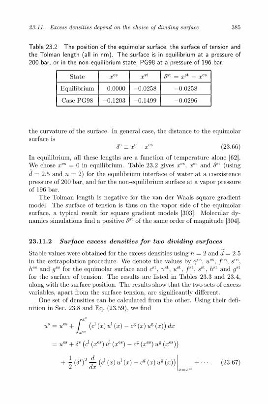
23.11. Excess densities depend on the choice of dividing surface 385
Table 23.2 The position of the equimolar surface, the surface of tension andthe Tolman length (all in nm). The surface is in equilibrium at a pressure of200 bar, or in the non-equilibrium state, PG98 at a pressure of 196 bar.
State xes xst δst = xst − xes
Equilibrium 0.0000 −0.0258 −0.0258
Case PG98 −0.1203 −0.1499 −0.0296
the curvature of the surface. In general case, the distance to the equimolarsurface is
δs ≡ xs − xes (23.66)
In equilibrium, all these lengths are a function of temperature alone [62].We chose xes = 0 in equilibrium. Table 23.2 gives xes, xst and δst (usingd = 2.5 and n = 2) for the equilibrium interface of water at a coexistencepressure of 200 bar, and for the non-equilibrium surface at a vapor pressureof 196 bar.
The Tolman length is negative for the van der Waals square gradientmodel. The surface of tension is thus on the vapor side of the equimolarsurface, a typical result for square gradient models [303]. Molecular dy-namics simulations find a positive δst of the same order of magnitude [304].
23.11.2 Surface excess densities for two dividing surfaces
Stable values were obtained for the excess densities using n = 2 and d = 2.5in the extrapolation procedure. We denote the values by γes, ues, f es, ses,hes and ges for the equimolar surface and cst, γst, ust, f st, sst, hst and gst
for the surface of tension. The results are listed in Tables 23.3 and 23.4,along with the surface position. The results show that the two sets of excessvariables, apart from the surface tension, are significantly different.
One set of densities can be calculated from the other. Using their defi-nition in Sec. 23.8 and Eq. (23.59), we find
us = ues +
∫ xs
xes
(cl (x) ul (x) − cg (x) ug (x)
)dx
= ues + δs(cl (xes)ul (xes) − cg (xes)ug (xes)
)
+1
2(δs)
2 d
dx
(cl (x) ul (x) − cg (x)ug (x)
)∣∣∣∣x=xes
+ · · · . (23.67)

386 Chapter 23. The Non-Equilibrium Two-Phase van der Waals Model
Table 23.3 The position and the excess densities of the equimolar surface.
xes γes ues fes ses hes ges
nm mJ/m2 mJ/m2 mJ/m2 µJ/K m2 mJ/m2 mJ/m2
EQ 0.0000 7.89510 85.5004 7.8951 138.17 77.605 0.0000
PG98 −0.1203 8.03148 85.2016 12.117 137.64 77.170 4.0852
PG99 −0.0607 7.96333 85.3480 10.012 137.90 77.385 2.0492
PG101 0.0620 7.82677 85.6583 5.7635 138.45 77.832 −2.0633
Pg102 0.1253 7.75832 85.8213 3.6167 138.74 78.063 −4.1416
TL98 0.5237 9.09685 90.9243 −7.1863 147.95 81.827 −16.283
TL99 0.2744 8.49571 88.1952 0.4412 143.00 79.699 −8.0545
TL101 −0.3042 7.29962 82.8788 15.091 133.53 75.579 7.7916
TL102 −0.6447 6.71485 80.3785 21.933 129.16 73.664 15.218
and similar expressions for the other excess densities. Since δs is very small,it is usually sufficient to only use the linear term of this expansion. Thisthen results in
cs = δs(cl − cg
), us = ues + δs
(clul − c gug
),
hs = hes + δs(clhl − c ghg
)ss = ses + δs
(clsl − cgsg
),
f s − gs = f es − ges + δs(clf l − c gfg
)− δs
(clµl − c gµg
)(23.68)
For ease of notation we have suppressed the fact that the differences ofthe extrapolated densities should be evaluated in xes. The reason that oneshould only give this relation for f s − gs and not for f s and gs separatelyfollows from their definition in Eq. (23.59). All relations in Eq. (23.68) werefound to apply in very good approximation.
23.11.3 The surface temperature from excess
density differences
From the autonomous nature of the surface, it follows that all linear expan-sion coefficients in Eq. (23.68) should have their equilibrium value at thetemperature of the surface. All excess densities for the equilibrium surfaceare functions of the temperature alone. The state of the surface is thereforegiven in terms of the temperature alone. By applying Eq. (23.68) to the

23.11. Excess densities depend on the choice of dividing surface 387
Table 23.4 The position and the excess densities of the surface of tension.
xst cst γst ust fst sst hst gst
nm µmol/m2 mJ/m2 mJ/m2 mJ/m2 µ J/m2K mJ/m2 mJ/m2
EQ −0.0258 −0.64280 7.89510 89.1927 42.350 83.402 81.298 34.455
PG98 −0.1499 −0.73912 8.03148 89.4138 51.752 74.602 81.382 43.721
PG99 −0.0885 −0.69133 7.96333 89.3034 47.077 78.967 81.340 39.114
PG101 0.0381 −0.59349 7.82677 89.0811 37.568 87.909 81.254 29.741
PG102 0.1033 −0.54344 7.75832 88.9682 32.731 92.484 81.210 24.973
TL98 0.5082 −0.40248 9.09685 93.4151 13.906 113.98 84.318 4.8086
TL99 0.2541 −0.51614 8.49571 91.2750 27.799 99.227 82.779 19.304
TL101 −0.3365 −0.78624 7.29962 87.2205 57.694 66.230 79.921 50.395
TL102 −0.6852 −0.95145 6.71486 85.4247 74.029 47.345 78.710 67.314
equilibrium surface, we find
cseq(Teq) = δseq(Teq)[cleq(Teq) − cgeq(Teq)]
useq(Teq) = ues
eq(Teq) + δseq(Teq)[cleq(Teq)u
leq(Teq) − cgeq(Teq)u
geq(Teq)]
= ueseq(Teq) + cseq(Teq)
[cleq(Teq)u
leq(Teq) − cgeq(Teq)u
geq(Teq)
cleq(Teq) − cgeq(Teq)
]
(23.69)
and similar expressions for hs, ss and f s − gs. When the system is notin equilibrium, the property of local equilibrium implies that the relationsin Eq. (23.69) remain valid, but now at the temperature of the surface.This means that for a surface in local equilibrium, the extrapolated bulkdensities must satisfy
cl − cg = cleq(Ts) − cg(T s)
clul − cgug = cleq(Ts)ul
eq(Ts) − cgeq(T
s)ugeq(T
s)(23.70)
and similar expressions for hs, ss and f s− gs. From knowledge of the molardensity difference in the non-equilibrium situation, one can find the sur-face temperature that gives the corresponding density difference at equilib-rium. This is equivalent to the statement that the linear coefficients in the

388 Chapter 23. The Non-Equilibrium Two-Phase van der Waals Model
expansion in Eq. (23.67) have their equilibrium value. Furthermore, it fol-lows that
cs(T s) = δs(T s)[cleq(Ts) − cgeq(T
s)]
us(T s, cs(T s)) = ues(T s) + δs(T s)[cleq(T
s)uleq(T
s) − cgeq(Ts)ug
eq(Ts)]
= ues(T s) + cs(T s)
[cleq(T
s)uleq(T
s) − cgeq(Ts)ug
eq(Ts)
cleq(Ts) − cgeq(T s)
]
(23.71)
and similar expressions for hs, ss and f s−gs. Also this is a good approxima-tion for all variables concerned. A better agreement can of course be foundby taking the nonlinear contributions in Eq. (23.67) along. For all practicalpurposes, Eq. (23.70) gives a simple and therefore very useful formula forthe surface temperature during evaporation or condensation.
23.12 The entropy balance and the excess
entropy production
We continue to verify the consistency of the integrated van der Waalssquare gradient model, with the framework of non-equilibrium thermody-namics for surfaces. The entropy balance of the surface in a stationarystate is [305]:
Jsl(xs) +J ′l
q (xs)
T l (xs)− Jsg(xs) −
J ′gq (xs)
T g (xs)= σs (23.72)
where the excess entropy production σs is given by:
σs =
∫ xout
xin
dx
J ′
q (x)d
dx
[1
T (x)
]− J ′g
q (x)d
dx
[1
T g (x)
]θ (xs − x)
−J ′lq (x)
d
dx
[1
T l (x)
]θ (x− xs)
(23.73)
It was shown that σs is the proper excess of σ(x) [108].The problem left is to show that the excess entropy production can be
written in the form given in Chapter 5. We use J ′q (x) = Jq − H(x)J ,
Eq. (23.50c) and neglect the small kinetic energy. The total heat flux Jq

23.12. The entropy balance and the excess entropy production 389
and the mass flux J are independent of x, and we can write
σs = Jq
∫ xout
xin
dx
d
dx
[1
T (x)
]− d
dx
[1
T g (x)
]θ (xs − x)
− d
dx
[1
T l (x)
]Θ (x− xs)
− J
∫ xout
xin
dx
H (x)
d
dx
[1
T (x)
]
−Hg (x)d
dx
[1
T g (x)
]Θ (xs − x) −H l (x)
d
dx
[1
T l (x)
]θ (x− xs)
= Je
[1
T l (xs)− 1
T g (xs)
]− J
∫ xout
xin
dx
H (x)
d
dx
[1
T (x)
]
−Hg (x)d
dx
[1
T g (x)
]Θ (xs − x) −H l (x)
d
dx
[1
T l (x)
]θ (x− xs)
(23.74)
In the second identity, we used the temperature and the extrapolated tem-peratures that are equal at the ends (x = xin or xout) of the box.
The Gibbs–Helmholtz equation for a constant normal pressure is:
H (x)d
dx
(1
T (x)
)=
d
dx
(µ (x)
T (x)
)(23.75)
By substituting Eq. (23.75) into Eq. (23.74), and using µ/T equal to µg/T g
or equal to µl/T l at the ends of the box, one finds
σs = Jq
[1
T l (xs)− 1
T g (xs)
]− J
∫ xout
xin
dx
d
dx
(µ (x)
T (x)
)
− d
dx
(µg (x)
T g(x)
)Θ (xs − x) − d
dx
(µl (x)
T l(x)
)Θ (x− xs)
= Jq
[1
T l (xs)− 1
T g (xs)
]− J
[µl (xs)
T l (xs)− µg (xs)
T g (xs)
](23.76)
which is the usual expression found using non-equilibrium thermodynamicsfor the excess entropy production, see Chapters 5 and 11 [4, 36, 38–40].
By eliminating the total heat flux in terms of the measurable heat fluxin the gas, we obtain
σs = J ′gq (xs)
[1
T l (xs)− 1
T g (xs)
]− J
[µl(T l (xs)) − µg(T l (xs))
T l (xs)
](23.77)

390 Chapter 23. The Non-Equilibrium Two-Phase van der Waals Model
Figure 23.6 The heat transfer coefficients, rsqq (solid lines) for three values of
α, and the kinetic theory value rs,kinqq (dashed line), as a function of the surfacetension.
which is Eq. (11.8) used in Chapter 11 to describe evaporation and con-densation. The expression containing the pressure and the vapor pressureof the liquid given in Eq. (11.13) follows from this expression. In derivingEq. (23.77) we used Eq. (23.75) for the vapor
Hg =d (µg/T )
d (1/T )(23.78)
In the derivation of Eq. (23.77) from Eq. (23.76), a term of the second orderin the thermodynamic forces is neglected.
23.13 Resistivities to heat and mass transfer
We have so far confirmed that the surface can be regarded as an autonomoussystem. Using the entropy production given in Eq. (23.77), we are now in aposition to give the linear force-flux relations from the non-equilibrium vander Waals square gradient model. We write them on the resistance form,as it was done also in Chapter 11:
1
T l (xs)− 1
T g (xs)= rsqqJ
′gq (xs) + rsqµJ
−µl(T l (xs)) − µg(T l (xs))
T l (xs)= rsµqJ
′gq (xs) + rsµµJ
(23.79)
The resistivities are of interest.†
†A common factor T l (xs) was absorbed in the resistivities in Refs. [36–40].

23.13. Resistivities to heat and mass transfer 391
Section 23.5 used the parameter α in Eq. (23.40) to determine the re-sistance to heat flow. In the numerical results quoted above, a constantvalue was used. The temperature profiles were sensitive to the choice ofthis constant. We shall now address the problem of how to choose α suchthat it reproduces the magnitude of the temperature difference across thesurface from kinetic theory [36] and non-equilibrium molecular dynamics.Non-equilibrium molecular dynamics simulations gave most of the resistiv-ity on the vapor side of the surface [40, 112]. In this section, we thereforeuse
α (T (x), c(x)) = α
(clcoex(Teq)
c(x)
)2
(23.80)
for the dependence of α on the concentration. The coefficient α on theright hand side is now kept constant in the numerical calculations. Theresistivities for heat and mass transfer were calculated for various conditionsas a function of this α [108]. Figure 23.6 illustrates various results for rsqq .Close to the critical point (γ = 0) all resistivities should approach zero.The values obtained numerically support this. Away from the critical point,the resistivities increased roughly proportional to α. The dashed curve inFig. 23.6 is obtained from kinetic theory, using Eq. (11.23), and has beenput in for comparison. Kinetic theory is only valid far from the criticalpoint.
Few experimental results near the triple point are available [160, 162]to fit rsqq and rsµµ. It was shown that these results could be described us-ing non-equilibrium thermodynamics [38]. The experimental results for thetransfer resistivities are about a factor of thirty larger than the correspond-ing kinetic theory-values. Part of the reason may be that convection dueto the Marangoni effect plays a role [306], see also [166] for a discussion.Recent molecular dynamics simulations done in our group for a long-rangeLennard-Jones potential give larger coupling coefficients, but certainly notlarge enough to explain the difference. The reason for the discrepancybetween kinetic theory and experiments is therefore as yet unclear.
The coupling coefficients rsqµ = rsµq found from the van der Waals squaregradient model, when we use α = 5 × 10⁻⁴, are much larger than thevalues given by kinetic theory. The heat of transfer q∗,s = −rsqµ/r
sqq is
about −7400 J/mol in the van der Waals model close to the triple point.The corresponding values found using NEMD simulations for the cut-off Lennard-Jones interaction give −9400 J/mol [167], the Lennard-Jonesspline potential gives −320 J/mol [40] and the cutoff Lennard-Jones inter-action for octane gives −1200 J/mol [112]. The value from kinetic the-ory is −363 J/mol [167]. It is surprising that the values differ so muchin magnitude.

392 Chapter 23. The Non-Equilibrium Two-Phase van der Waals Model
23.14 Concluding comments
The non-equilibrium van der Waals square gradient model has been foundto give a simple and robust method to describe the liquid-vapor inter-face. The model gives continuous profiles for all thermodynamic variablesthrough the interface region. While the model itself is not autonomous, itleads to an autonomous description of the surface in terms of the excessdensities. A number of definitions of the surface temperature was givenand it was verified that they all gave the same value of this temperature.The autonomous description treats the surface as a separate thermody-namic system [62, 93–95] and is simpler than the description suggested byDefay and coworkers [96]. The model opens up possibilities to calculateand analyze the surface resistivities to heat and mass transfer.

References
[1] L. Waldmann. Non-equilibrium thermodynamics of boundary condi-tions. Z. Naturforschung, 22a:1269–1280, 1967.
[2] D. Bedeaux, A.M. Albano and P. Mazur. Boundary conditions andnonequilibrium thermodynamics. Physica A, 82:438–462, 1976.
[3] A.M. Albano and D. Bedeaux. Non-equilibrium electrothermo-dynamics of polarizable multicomponent fluids with an interface.Physica A, 147:407–435, 1987.
[4] D. Bedeaux. Nonequilibrium thermodynamics and statistical physicsof surfaces. Adv. Chem. Phys., 64:47–109, 1986.
[5] D. Bedeaux and J. Vlieger. Optical Properties of Surfaces. ImperialCollege University Press, London, 1st edition, 2002.
[6] D. Bedeaux and J. Vlieger. Optical Properties of Surfaces. ImperialCollege University Press, London, 2nd revised edition, 2004.
[7] W. Thomson (Lord Kelvin). Mathematical and Physical Papers. Col-lected from different Scientific Periodicals from May, 1841, to thePresent Time, Vol. II. Cambridge University Press, London, 1884.
[8] L. Onsager. Reciprocal relations in irreversible processes. I. Phys.Rev., 37:405–426, 1931.
[9] L. Onsager. Reciprocal relations in irreversible processes. II. Phys.Rev., 38:2265–2279, 1931.
[10] H. Hemmer, H. Holden and S. Kjelstrup Ratkje, editors. The CollectedWorks of Lars Onsager. World Scientific, Singapore, 1996.
[11] J. Meixner. Zur Thermodynamik der Thermodiffusion. Ann. Physik5. Folge, 39:333–356, 1941.
[12] J. Meixner. Reversible Bewegungen von Flüssigkeiten und Gasen.Ann. Physik 5. Folge, 41:409–425, 1942.
[13] J. Meixner. Zur Thermodynamik der irreversibelen Prozesse in Gasenmit chemisch reagirenden, dissozierenden und anregbaren Komponen-ten. Ann. Physik 5. Folge, 43:244–270, 1943.
[14] J. Meixner. Zur Thermodynamik der irreversibelen Prozesse.Zeitschr. Phys. Chem. B, 53:235–263, 1943.
393

394 References
[15] I. Prigogine. Etude Thermodynamique des Phenomenes Irreversibles.Desoer, Liege, 1947.
[16] P. Mitchell. Coupling of phosphorylation to electron and hydrogentransfer by a chemi-osmotic type of mechanism. Nature (London),191:144–148, 1961.
[17] K.G. Denbigh. The Thermodynamics of the Steady State. Methuen,London, 1951.
[18] I. Prigogine. Thermodynamics of Irreversible Processes. Charles C.Thomas, Springfield, 1st edition, 1955.
[19] S.R. de Groot and P. Mazur. Non-Equilibrium Thermodynamics.North-Holland, Amsterdam, 1962.
[20] S.R. de Groot and P. Mazur. Non-Equilibrium Thermodynamics.Dover, London, 1984.
[21] R. Haase. Thermodynamics of Irreversible Processes. Addison-Wesley,Reading, MA, 1969.
[22] R. Haase. Thermodynamics of Irreversible Processes. Dover, London,1990.
[23] A. Katchalsky and P. Curran. Nonequilibrium Thermodynamics inBiophysics. Harvard University Press, Cambridge, Massachusetts,1975.
[24] S.R. Caplan and A. Essig. Bioenergetics and Linear Non-EquilibriumThermodynamics — The Steady State. Harvard University Press,Cambridge, Massachusetts, USA, 1983.
[25] H.V. Westerhoff and K. van Dam. Thermodynamics and Control ofBiological Free-Energy Transduction. Elsevier, Amsterdam, 1987.
[26] K. S. Førland, T. Førland and S. Kjelstrup Ratkje. Irreversible Ther-modynamics. Theory and Application. Wiley, Chichester, 1st edition,1988.
[27] K. S. Førland, T. Førland, and S. Kjelstrup. Irreversible Thermo-dynamics. Theory and Application. Tapir, Trondheim, Norway, 3rdedition, 2001.
[28] S. Kjelstrup and D. Bedeaux. Elements of Irreversible Thermodynam-ics for Engineers. Int. Centre of Applied Thermodynamics, Instanbul,Turkey, 1st edition, 2001.
[29] S. Kjelstrup, D. Bedeaux and E. Johannessen. Elements of Irre-versible Thermodynamics for Engineers. Tapir Akademiske Forlag,Trondheim, Norway, 2nd revised edition, 2006.
[30] D.D. Fitts. Nonequilibrium Thermodynamics. McGraw-Hill, NewYork, 1962.
[31] G.D.C. Kuiken. Thermodynamics for Irreversible Processes. Wiley,Chichester, 1994.
References 395
[32] Y.P. Pao. Application of kinetic theory to problem of evaporation andcondensation. Phys. Fluids, 14:306–312, 1971.
[33] Y.P. Pao. Temperature and density jumps in kinetic theory of gasesand vapors. Phys. Fluids, 14:1340–1346, 1971.
[34] J.W. Cipolla Jr., H. Lang and S.K. Loyalka. Kinetic theory of con-densation and evaporation. II. J. Chem. Phys., 61:69–77, 1974.
[35] C. Cercignani. Strong evaporation of a polyatomic gas. In S. Fisher,editor, Rarified Gas Dynamics, Vol. 74, pages 305–320, New York,1981. Progr. Astronaut. Aeronaut. AIAA.
[36] D. Bedeaux, L.F.J. Hermans and T. Ytrehus. Slow evaporation andcondensation. Physica A, 169:263–280, 1990.
[37] D. Bedeaux, J.A.M. Smit, L.F.J. Hermans and T. Ytrehus. Slow evap-oration and condensation. 2. A dilute mixture. Physica A, 182:388–418, 1992.
[38] D. Bedeaux and S. Kjelstrup. Transfer coefficients for evaporation.Physica A, 270:413–426, 1999.
[39] A. Røsjorde, D.W. Fossmo, D. Bedeaux, S. Kjelstrup and B. Haf-skjold. Non-equilibrium molecular dynamics simulations of steady-state heat and mass transport in condensation I: Local equilibrium.J. Colloid Interface Sci., 232:178–185, 2000.
[40] A. Røsjorde, D. Bedeaux, S. Kjelstrup and B. Hafskjold. Non-equilibrium molecular dynamics simulations of steady-state heat andmass transport in condensation II: Transfer coefficients. J. ColloidInterface Sci., 240:355–364, 2001.
[41] V.I. Roldughin and V.M. Zhdanov. Non-equilibrium thermodynam-ics and kinetic theory of gas mixtures in the presence of interfaces.Advances in Colloid and Interface Science, 98:121–215, 2002.
[42] R. Krishna and J.A. Wesselingh. The Maxwell–Stefan approach tomass transfer. Chem. Eng. Sci., 52:861–911, 1997.
[43] D. Bedeaux and P. Mazur. Mesoscopic non-equilibrium thermody-namics for quantum systems. Physica A, 298:81–100, 2001.
[44] W. Muschik, C. Papenfuss and H. Ehrentraut. A sketch of continuumthermodynamics. J. Non-Newtonian Fluid Mech., 96:255–290, 2001.
[45] I. Pagonabarraga and J.M. Rubi. Derivation of the Langmuir ad-sorption equation from non-equilibrium thermodynamics. Physica A,188:553–567, 1992.
[46] I. Pagonabarraga, A. Perez-Madrid and J.M. Rubi. Fluctuating hy-drodynamics approach to chemical reactions. Physica A, 237:205–219,1997.
[47] D. Reguera and J.M. Rubi. Kinetic equations for diffusion in thepresence of entropic barriers. Phys. Rev. E, 64:061106 (1–8), 2001.

396 References
[48] D. Reguera and J.M. Rubi. Nonequilibrium translational-rotationaleffects in nucleation. J. Chem. Phys., 115:7100–7106, 2001.
[49] T. Tsuruta and G. Nagayama. DSMC analysis of interface mass trans-fer in evaporation/condensation based on molecular dynamics study.Thermal Science & Engineering, 10:9–15, 2002.
[50] D. Bedeaux, S. Kjelstrup and J.M. Rubi. Nonequilibrium trans-lational effects in evaporation and condensation. J. Chem. Phys.,119:9163–9170, 2003.
[51] J.M. Rubi and S. Kjelstrup. Mesoscopic nonequilibrium thermody-namics gives the same thermodynamic basis to Butler–Volmer andNernst equations. J. Phys. Chem. B, 107:13471–13477, 2003.
[52] S. Kjelstrup, J.M. Rubi and D. Bedeaux. Energy dissipation in slip-ping biological pumps. Phys. Chem. Chem. Phys., 7:4009–4018, 2005.
[53] S. Kjelstrup, J.M. Rubi and D. Bedeaux. Active transport: Kineticdescription on thermodynamic grounds. J. Theoretical Biology, 234:7–12, 2005.
[54] J.M. Rubi, D. Bedeaux and S. Kjelstrup. Thermodynamics for smallmolecule stretching experiments. J. Phys. Chem. B, 110:12733–12737,2006.
[55] V.P. Carey. Statistical Thermodynamics and Microscale Thermo-physics. Cambridge University Press, Cambridge, UK, 1999.
[56] D. Kondepudi and I. Prigogine. Modern Thermodynamics. From HeatEngines to Dissipative Structures. Wiley, Chichester, 1998.
[57] H.C. Öttinger. Beyond Equilibrium Thermodynamics. Wiley-Interscience, Hoboken, 2005.
[58] E.M. Hansen and S. Kjelstrup. Application of nonequilibrium ther-modynamics to the electrode surfaces of aluminium electrolysis cells.J. Electrochem. Soc., 143:3440–3447, 1996.
[59] G. Bertrand and R. Prud’homme. Possibilitiess of Surface reactionCoupling with Transport Phenomena. Int. J. Quantum Chemistry,7:159–168, 1977.
[60] G. Bertrand. Active Transport by Membranes: An Example of aGeneral Property of Reactive Surfaces. J. Non-Equilib. Thermodyn.,6:165–172, 1981.
[61] D. Bedeaux and S. Kjelstrup. Heat, mass and charge transport andchemical reactions at surfaces. Int. J. of Thermodynamics, 8:25–41,2005.
[62] J.W. Gibbs. The Scientific Papers of J.W. Gibbs. Dover, New York,1961.
[63] E.A. Guggenheim. The conceptions of electrical potential differencebetween two phases and the individual activities of ions. J. Phys.Chem., 33:842–849, 1928.

References 397
[64] D. Jou, J. Casas-Vázquez and G. Lebon. Extended Irreversible Ther-modynamics. Springer-Verlag, Berlin, 2nd edition, 1996.
[65] B. Hafskjold and S. Kjelstrup Ratkje. Criteria for local equilibrium ina system with transport of heat and mass. J. Stat. Phys., 78:463–494,1995.
[66] F. Bresme, B. Hafskjold and I. Wold. Nonequilibrium molecular dy-namics study of heat conduction in ionic systems. J. Phys. Chem.,100:1879–1888, 1996.
[67] J. Xu, S. Kjelstrup, D. Bedeaux, A. Røsjorde and L. Rekvig. Ver-ification of Onsager’s reciprocal relations for evaporation and con-densation using non-equilibrium molecular dynamics simulations. J.Colloid Interface Sci., 299:452–463, 2006.
[68] J. Xu, S. Kjelstrup and D. Bedeaux. Molecular dynamics simulationsof a chemical reaction; conditions for local equilibrium in a tempera-ture gradient. Phys. Chem. Chem. Phys., 8:2017–2027, 2006.
[69] R. Taylor and R. Krishna. Multicomponent Mass Transfer. Wiley,New York, 1993.
[70] E.L. Cussler. Diffusion, Mass Transfer in Fluid Systems. Cambridge,2nd edition, 1997.
[71] D.G. Miller. Thermodynamics of irreversible processes. The experi-mental verification of the Onsager reciprocal relations. Chem. Revs.,60:15–37, 1960.
[72] D.G. Miller. Application of irreversible thermodynamics to elec-trolyte solutions. I. Determination of ionic transport coefficients lij forisothermal vector transport processes in binary electrolyte systems.J. Phys. Chem., 70:2639–2659, 1966.
[73] D.G. Miller. Application of irreversible thermodynamics to electrolytesolutions. II. Ionic coefficients lij for isothermal vector transport pro-cesses in ternary systems. J. Phys. Chem., 71:616–632, 1967.
[74] D.G. Miller and M.J. Pikal. A test of the Onsager reciprocal relationsand a discussion of the ionic isothermal vector transport coefficientlij for aqueous AgNO3 at 25oC. J. Solution Chem., 1:111–130, 1972.
[75] M. Spallek, H.G. Hertz, S. Kashammer, H. Weingärtner. Ternarydiffusion and onsager reciprocity relations in aqueous ZnCl2+KCland CdCl2+KCl revisited. Ber. Bunsenges. Phys. Chem., 96:764–769,1995.
[76] O. Annunziata, L. Paduano, A.J. Pearlstein, D.G. Miller and J.G. Al-bright. Extraction of thermodynamic data from ternary diffusion coef-ficients. Use of precision diffusion measurements for aqueous lysozymechloride-NaCl at 25o to determine the change in lysozyme chloridechemical potential with increasing NaCl concentration well into thesupersaturation region. J. Am. Chem. Soc., 122:5916–5928, 2000.

398 References
[77] T.S. Brun and D. Vaula. Correlation of measurements of electroosmo-sis and streaming potentials in ion exchange membranes. Ber. Bun-senges. Physik. Chem., 71:824–829, 1967.
[78] B. Flem, S. Kjelstrup and Å. Sterten. Peltier heats in cryolite meltswith alumina. Light Metals, pp. 203–209, 1996.
[79] B. Flem. Peltier Heats in Cryolite Melts with Alumina. PhD thesis,Department of Physical Chemistry, Norwegian Institute of Technol-ogy, Trondheim, 1996.
[80] B. Flem, Q. Xu, S. Kjelstrup and Å. Sterten. Thermoelectric powersof cells with NaF-AlF3-Al2O3 melts. J. Non-Equilib. Thermodyn.,26:125–151, 2001.
[81] A.K. Meland, D. Bedeaux and S. Kjelstrup. A Gerischer phase ele-ment in the impedance diagram of the polymer electrolyte fuel cellanode. J. Phys. Chem. B, 109:21380–21388, 2005.
[82] J. Szargut, D.R. Morris and F.R. Steward. Exergy Analysis of Ther-mal, Chemical and Metallurgical Processes. Hemisphere, New York,1988.
[83] K.G. Denbigh. The second-law efficiency of chemical processes. Chem.Engng. Sci., 6:1–9, 1956.
[84] A. Bejan. Entropy Generation Through Heat and Fluid Flow. Wiley,New York, 1982.
[85] A. Bejan. Entropy generation minimization: The new thermodynam-ics of finite-size devices and finite-time processes. J. Appl. Phys.,79:1191–1218, 1996.
[86] S. Kjelstrup Ratkje and J. de Swaan Arons. Denbigh revisited: Reduc-ing lost work in chemical processes. Chem. Eng. Sci., 50:1551–1560,1995.
[87] G.M. de Koeijer, E. Johannessen and S. Kjelstrup. The second lawoptimal path of a four-bed SO2 converter with five heat exchangers.Energy, 29:525–546, 2004.
[88] E. Johannessen and S. Kjelstrup. Minimum entropy production ratein plug flow reactors: An optimal control problem solved for SO2
oxidation. Energy, 29:2403–2423, 2004.[89] L. Nummedal, A. Røsjorde, E. Johannessen and S. Kjelstrup. Sec-
ond law optimization of a tubular steam reformer. Chem. Eng. Proc.,44:429–440, 2005.
[90] A. Røsjorde and S. Kjelstrup. The second law optimal state of adiabatic binary tray distillation column. Chem. Eng. Sci., 60:1199–1210, 2005.
[91] E. Johannessen and S. Kjelstrup. A highway in state space for reactorswith minimum entropy production. Chem. Eng. Sci, 60:3347–3361,2006.
References 399
[92] A. Zvolinschi, E. Johannessen and S. Kjelstrup. The second law opti-mal operation of a paper drying machine. Chem. Eng. Sci., 61:3653–3662, 2006.
[93] J.S. Rowlinson and B. Widom. Molecular Theory of Capillarity. Ox-ford University Press, Oxford, 1982.
[94] G. Bakker. Kapillarität und Oberflachespannung. In W. Wien, F.Harms and H. Lenz, editors, Handbuch der Experimentalphysik,Vol. 6, Chapter 10. Akad. Verlag, Leipzig, Germany, 1928.
[95] E.A. Guggenheim. Thermodynamics. North-Holland, Amsterdam,7th edition, 1985.
[96] R. Defay and I. Prigogine. Surface Tension and Absorption. Long-mans and Green, London, 1966.
[97] P.W. Atkins. Physical Chemistry. Oxford University Press, Oxford,6th edition, 1998.
[98] E.M. Blokhuis and D. Bedeaux. Microscopic expressions for the rigid-ity constants of a simple liquid-vapour interface. J. Chem. Phys.,95:6986–6988, 1991.
[99] E.M. Blokhuis and D. Bedeaux. Derivation of microscopic expressionsfor the rigidity constants of a simple liquid-vapour interface. PhysicaA, 184:42–70, 1992.
[100] E.M. Blokhuis and D. Bedeaux. The pressure tensor of a sphericalinterface. J. Chem. Phys., 97:3576–3586, 1992.
[101] E.M. Blokhuis and D. Bedeaux. Van der Waals theory of curves sur-faces. Mol. Phys., 80:705–720, 1993.
[102] E.M. Blokhuis and D. Bedeaux. Microscopic theories of curves liquidsurfaces. Heterogeneous Chemistry Reviews, 1:55–68, 1994.
[103] J. Groenewold and D. Bedeaux. Microscopic integral relations for thecurvature dependent surface tension in a two-phase multi-componentsystem. Physica A, 214:356–378, 1995.
[104] J.D. van der Waals. The thermodynamic theory of capillarity underthe hypothesis of a continuous variation of density (in Dutch). Ver-handel. Konink. Akad. Weten. Amsterdam, 1:56, 1893.
[105] J.W. Cahn and J.E. Hillard. Free energy of nonuniform systems. I.Interfacial free energy. J. Chem. Phys., 28:258–267, 1958.
[106] D. Bedeaux, E. Johannessen and A. Røsjorde. The non-equilibriumvan der Waals square gradient model. I. The model and its numericalsolution. Physica A, 330:329–353, 2003.
[107] E. Johannessen and D. Bedeaux. The non-equilibrium van der Waalssquare gradient model. II. Local equilibrium and the Gibbs surface.Physica A, 330:354–372, 2003.
[108] E. Johannessen and D. Bedeaux. The non-equilibrium van der Waals

400 References
square gradient model. III. Heat and mass transfer coefficients. Phys-ica A, 336:252–270, 2004.
[109] J.M. Ortiz de Zárate and J.V. Sengers. Hydrodynamic Fluctuationsin Fluids and Fluid Mixtures. Elsevier, Amsterdam, 2006.
[110] I. Prigogine. Le domain de validité de la thermodynamique des phe-nomenes irreversibles. Physica, 15:272–283, 1949.
[111] F. Bresme. Equilibrium and nonequilibrium molecular simulations ofthe central force model of water. J. Chem. Phys., 115:7564–7574,2001.
[112] J.-M. Simon, S. Kjelstrup, D. Bedeaux and B. Hafskjold. Thermal fluxthrough a surface of n-octane. A non-equilibrium molecular dynamicsstudy. J. Phys. Chem. B, 108:7186–7195, 2004.
[113] B.J.A. Zielinska and D. Bedeaux. A hydrodynamic theory for fluc-tuations around equilibrium of a liquid-vapour interface. Physica A,112:265–286, 1982.
[114] R.H. Perry and D.W. Green. Perry’s Chemical Engineers Handbook.McGraw-Hill, New York, 7th edition, 1997.
[115] J. Ross and P. Mazur. Some deductions from a statistical mechanicaltheory of chemical kinetics. J. Chem. Phys., 35:19–28, 1961.
[116] Y. Demirel. Non-equilibrium Thermodynamics. Transport and RateProcesses in Physical and Biological Systems. Elsevier, Amsterdam,2002.
[117] I. Prigogine. Thermodynamics of Irreversible Processes. Interscience,New York, 2nd edition, 1961.
[118] R. S. Schechter. The Variational Method in Engineering. McGraw-Hill, New York, 1967.
[119] S. Kjelstrup Ratkje, E. Sauar, E.M. Hansen, K. Lien and B. Hafskjold.Analysis of entropy production rates for design of distillation columns.Ind. Eng. Chem. Res., 34:3001–3007, 1995.
[120] B. Andresen, P. Salamon and R. S. Berry. Thermodynamics in finitetime. Physics Today, September:62–70, 1984.
[121] J.R. Welty, C.E. Wicks and R.E. Wilson. Fundamentals of Momen-tum, Heat and Mass Transfer. Wiley, Chichester, UK, 3rd edition,1984.
[122] M. J. Moran and H. N. Shapiro. Fundamentals of Engineering Ther-modynamics. Wiley, New York, 2nd edition, 1993.
[123] D. Bedeaux and S. Kjelstrup. Non-equilibrium thermodynamics forsurfaces. Lecture notes of NorFA Summer School, Chalmers Univer-sity of Technology, Gøteborg, Sweden, September 2002.
[124] D. Bedeaux and S. Kjelstrup. Irreversible thermodynamics — a toolto describe phase transitions far from global equilibrium. Chem. Eng.Sci., 59:109–118, 2004.
References 401
[125] D. Bedeaux, S. Kjelstrup, L. Zhu and G.J.M. Koper. Non-equilibriumthermodynamics. A tool to describe heterogeneous catalysis. Phys.Chem. Chem. Phys., 8:5421–5427, 2006.
[126] A.M. Albano, D. Bedeaux and J. Vlieger. On the description of inter-facial electromagnetic properties using singular fields, charge densityand currents at a dividing surface. Physica A, 102:105–119, 1980.
[127] D. Ronis, D. Bedeaux and I. Oppenheim. On the derivation of dy-namical equations for a system with an interface. I. General theory.Physica A, 90:487–506, 1978.
[128] D. Ronis and I. Oppenheim. On the derivation of dynamical equationsfor a system with an interface. II. The gas-liquid interface. PhysicaA, 90:487–506, 1983.
[129] D. Bedeaux and S. Kjelstrup Ratkje. The dissipated energy of elec-trode surfaces. Temperature jumps from coupled transport processes.J. Electrochem. Soc., 136:767–779, 1996.
[130] S. Kjelstrup and D. Bedeaux. Jumps in electric potential and in tem-perature at the electrode surfaces of the solid oxide fuel cell. PhysicaA, 244:213–226, 1997.
[131] Y.D. Shikhmurzaev. The moving contact line on a smooth solid sur-face. Int. J. Multiphase Flow, 19:589–610, 1993.
[132] D. Bedeaux. Nonequilibrium thermodynamic description of the three-phase contact line. J. Chem. Phys., 120:3744–3748, 2004.
[133] Y.D. Shikhmurzaev. Moving contact lines in liquid/liquid/solid sys-tems. J. Fluid Mech., 334:211–249, 1997.
[134] B.D. Coleman and C. Truesdell. On the reciprocal relations of On-sager. J. Chem. Phys., 53:28–31, 1960.
[135] J. Wei. Irreversible thermodynamics in engineering. Ind. Eng. Chem.,58:55–60, 1974.
[136] I. Prigogine. From being to becoming. Time and complexity in thephysical sciences. W.H. Freeman, San Francisco, 1980.
[137] P. Curie. Oeuvres. (Paris), p. 118, 1908.[138] R. B. Bird, W. E. Stewart and E. N. Lightfoot. Transport Phenomena.
Wiley, Chichester, UK, 1960.[139] H.J.V. Tyrell and K.R. Harris. Diffusion in Liquids. A theoretical and
experimental study. Butterworths, London, 1984.[140] S. Killie, B. Hafskjold, O. Borgen, S. Kjelstrup Ratkje and E. Hovde.
High pressure diffusion measurements by Mach-Zender interferome-try. AIChE J., 37:142–146, 1991.
[141] C.A. Angell. Supercooled Water. In F. Franks, editor, Water a com-prehensive treatise; Water and aqueous solutions at subzero tempera-tures, Vol. 7. Plenum Press, New York, USA, 1982.

402 References
[142] W.H. Furry, R.C. Jones and L. Onsager. On the theory of isotopeseparation by thermal diffusion. Phys. Rev., 55:1083–1095, 1939.
[143] A. Lunden. In A. Lodding and T. Lagerwall, editors, Atomic Trans-port in Solids and Liquids, Thermomigration of chemical compo-nents and isotopes in solid and molten salts, pp. 302–308. Verlagder Zeitschrift für Naturforschung, Tübingen, 1971.
[144] B. Rousseau, C. Niete-Draghi and J. Bonet Avalos. The role of themolecular association in the change of the sign of the soret coefficientin aquous mixtures. Europhysics Letters, 67:976–982, 2004.
[145] L.J.T.M. Kempers. A comprehensive thermodynamic theory of thesoret effect in a multicomponent gas, liquid or solid. J. Chem. Phys.,115:6330–6341, 2001.
[146] A.G. Guy. Prediction of thermal diffusion in binary mixtures of non-electrolyte liquids by the use of nonequilibrium thermodynamics. Int.J. Thermophys., 7:563–572, 1986.
[147] T. Holt, E. Lindeberg and S. Kjelstrup Ratkje. The effect of gravityand temperature gradients on methane distribution in oil reservoirs.SPE-paper no. 1176, 1983.
[148] J.N. Agar. In P. Delahay, editor, Advances in Electrochemistry andElectrochemical Engineering, Vol. 3, Thermogalvanic cells. Inter-science, New York, 1963.
[149] J.M. Kincaid, X. Li and B. Hafskjold. Nonequilibrium molecular dy-namics calculation of the thermal diffusion factor. Fluid Phase Equil.,76:113–121, 1992.
[150] L. Zhu and G. Frens. Indications for a surface temperature excess inheterogeneous catalysis. J. Phys. Chem. B, 110:18307–18312, 2006.
[151] L. Zhu, G.J.M. Koper and D. Bedeaux. Heats of transfer in the dif-fusion layer before the surface and the surface temperature for a cat-alytic hydrogen oxidation (H2 + 1
2 O2 → H2O) reaction. J. Phys.Chem. A, 110:4080–4088, 2006.
[152] E.M. Hansen. Modeling of Aluminium Electrolysis Cells Using Non-Equilibrium Thermodynamics. PhD thesis, University of Leiden, Lei-den, The Netherlands, 1997.
[153] T.C. Harman and J.M. Honig. Thermoelectric and ThermomagneticEffects and Applications. McGraw-Hill, New York, 1967.
[154] V.E. Zinoviev. Thermophysical Properties of Metals at High Temper-atures. Metallurgiya, Moscov, 1989.
[155] R.W. Cahn, editor. Physical Metallurgy. North-Holland, Amsterdam,1965.
[156] J.O’M. Bockris and D.M. Drazic. Electro-chemical Science. Taylor &Francis, London, 1972.
[157] Magnar Ottøy. Mass and Heat Transfer in Ion-Exchange Membranes.

References 403
PhD thesis, Norwegian University of Science and Technology, De-partment of Physical Chemistry, Trondheim, Norway, 1996. ISBN82-7119-933-1, ISSN 0802-3271.
[158] J.L. Jackson. Charge neutrality in electrolyte solutions and the liquidjunction potential. J. Phys. Chem., 78:2060–2064, 1974.
[159] H.S. Harned and B.B. Owen. Physical Chemistry of Electrolytic So-lutions. Reinhold, New York, 3rd edition, 1958.
[160] G. Fang and C.A. Ward. Temperature measured close to the interfaceof an evaporating liquid. Phys. Rev. E, 59:417–428, 1999.
[161] G. Fang and C.A. Ward. Examination of the statistical rate theoryexpression for liquid evaporation rates. Phys. Rev. E, 59:441–453,1999.
[162] G. Fang. Rate of liquid evaporation: Statistical rate theory approach.PhD thesis. Graduate Department Mechanical and Industrial Engi-neering, University of Toronto, Canada, 1999.
[163] C.T. Mills and L.F. Phillips. Onsager heat of transport at the aniline-vapour interface. Chem. Phys. Letters, 366:279–283, 2002.
[164] R.A. James and L.F. Phillips. Onsager heat of transport for watervapour at the surface of glycerol-water mixtures. Chem. Phys. Letters,425:49–52, 2006.
[165] F. Graner, R.M. Bowley and P. Nozieres. The growth-kinetics of He-3crystals. J. Low Temperature Physics, 80:113–133, 1990.
[166] M. Bond and H. Struchtrup. Mean evaporation and condensation co-efficients based on energy dependent condensation probability. Phys.Rev. E, 70:061605 (21 pages), 2004.
[167] S. Kjelstrup, T. Tsuruta and D. Bedeaux. The inverted temperatureprofile across a vapour/liquid surface analyzed by molecular computersimulations. J. Colloid Interface Sci., 256:451–461, 2002.
[168] J.W. Cipolla Jr., H. Lang and S.K. Loyalka. Temperature and PartialPressure Jumps During Evaporation and Condensation of a Multi-component Mixture. In Beeker and Fiebig, editors, Rarified Gas Dy-namics, Vol. II, pages F.4–1 to F.4–10. DFVLR-Press, Portz-Wahn,Germany, 1974.
[169] T. Ytrehus. Molecular-flow effects in evaporation and condensationat interfaces. Multiphase Science and Technology, 9:205–327, 1997.
[170] J. Ge, S. Kjelstrup, D. Bedeaux, J.M. Simon and B. Rousseau. Coef-ficients for evaporation of a system with a Lennard-Jones long rangespline potential. Phys. Rev. E, in press, 2007.
[171] M.-L. Olivier, J.-D. Rollier and S. Kjelstrup. Equilibrium propertiesand surface transfer coefficients from molecular dynamics simulationsof two-component fluids. Colloids and Surfaces A: Physicochem. Eng.Aspects, 210:199–222, 2002.

404 References
[172] T. Tsuruta and G. Nagayama. Interphase mass transfer rate betweenliquid and vapor based on molecular dynamics study. In G.J. Hwang,editor, Proceed. 11th Int. Symp. on Transport Phenomena, pp. 527–532, Hsinchu, Taiwan, 1998. Tsing Hua University.
[173] L.F. Phillips. Onsager heat of transport as a consequence of detailedbalance at the gas-liquid interface. Chem. Phys. Letters, 396:350–352,2004.
[174] D.R. Lide. CRC Handbook of Chemistry and Physics. CRC Press,New York, 78th edition, 1997.
[175] S. Kjelstrup and G. de Koeijer. Transport equations for distillationof ethanol and water from the entropy production rate. Chem. Eng.Science, 58:1147–1161, 2003.
[176] P.N. Shankar and M.D. Despande. On the temperature distibutionin a liquid-vapour phase change between plane liquid surfaces. Phys.Fluids A, 2:1030–1038, 1990.
[177] J.A. Wesselingh and R. Krishna. Mass Transfer in MulticomponentMixtures. Delft University Press, Delft, 2000.
[178] L.J.T.M. Kempers. A thermodynamic theory of the Soret effect in amulticomponent liquid. J. Phys. Chem., 90:6541–6548, 1989.
[179] M. Martin. Materials in thermodynamic potential gradients. PureAppl. Chem., 75:889–903, 2003.
[180] I.V. Belova, M.J. Brown and G.E. Murch. Analysis of kinetic demix-ing in a mixed oxide (A,B)O in an oxygen potential gradient. ActaMaterialia, 51:1821–1826, 2003.
[181] I.V. Belova, M.J. Brown and G.E. Murch. Analysis of kinetic demix-ing of (A,B)O oxides in an electric field and an oxygen potentialgradient. Solid State Ionics, 167:175–182, 2004.
[182] M.J. Brown, I.V. Belova and G.E. Murch. Prediction of a kineticdemixing in a quarternary mixed oxide (A,B,C)O in an oxygen po-tential gradient. Phil. Mag., 86:1855–1865, 2003.
[183] M. Palcut. Kinetic demixing in oxygen conducting oxide exposed tochemical potential gradient. Technical report, Norwegian Universityof Science and Technology, 2005.
[184] S. Kjelstrup, D. Bedeaux and E.M. Hansen. Surface contributions toemf and half cell potentials of non-isothermal cells. Periodica Poly-technica Ser. Chem. Eng., 41:11–27, 1997.
[185] V. Sharivker, S. Kjelstrup Ratkje and B. Cleaver. Determination ofthe entropy of molten polysulfides. Electrochim. Acta, 41:2381–2384,1996.
[186] B. Cleaver and V.S. Sharivker. Asymmetric thermal effects in high-temperature cells with solid electrolytes. J. Electrochem. Soc. 1995,142:3409–3413, 1995.

References 405
[187] Q. Xu and S. Kjelstrup. Reversible heat effects in the aluminiumelectrolysis. Light Metals, pages 539–546, 1998.
[188] Y. Ito, H. Kaiya, S. Yoshizawa, S. Kjelstrup Ratkje and T. Førland.Electrode heat balances of electrochemical cells: Application to waterelectrolysis. J. Electrochem. Soc., 131:2504–2509, 1984.
[189] S. Kjelstrup Ratkje, H. Rajabu and T. Førland. Transference coeffi-cients and transference numbers in molten salt mixtures relevant forthe aluminium electrolysis. Electrochim. Acta, 38:415–423, 1993.
[190] E. M. Hansen, E. Egner and S. Kjelstrup. Peltier effects in electrodecarbon. Metall. and Mater. Trans. B, 29:69–76, 1998.
[191] T. Ikeshoji and S. Kjelstrup Ratkje. Thermoelectric power of a cellwith complex formation. J. Electrochem. Soc., 133:1107–1113, 1986.
[192] S. Kjelstrup, E. Olsen and J. Qian. The peltier heating of aluminium,oxygen and carbon — carbon dioxide electrodes in an electrolyte ofsodium and aluminium fluorides saturated with alumina. Electrochim.Acta, 46:1141–1150, 2001.
[193] J.N. Agar and W.G. Breck. Thermal diffusion in non-isothermal cells.1. Theoretical relations and experiments of solutions of thallous salts.Trans. Faraday Soc., 53:167–178, 1956.
[194] V. Blinov, S. Kjelstrup, D. Bedeaux and V.S. Sharivker. The roleof the transported entropy of lead in partially thermostatted andadiabatic cells. J. Electrochem. Soc., 148:364–371, 2001.
[195] S. Kjelstrup Ratkje, V.S. Sharivker and B. Cleaver. Reversible heat ef-fects in high temperature batteries: Transported entropy and Thom-son coefficients in cells with β-alumina. Electrochim. Acta, 39:2659–2664, 1994.
[196] S. Kjelstrup Ratkje, T. Ikeshoji and K. Syverud. Heat and internalenergy changes at electrodes and junctions in thermocells. J. Elec-trochem. Soc., 137:542–560, 1990.
[197] A. Grimstvedt, S. Kjelstrup Ratkje and T. Førland. Theory of thermo-cells. Transported entropies and heat of transfer in sulfate mixtures.J. Electrochem. Soc., 141:1236–1241, 1994.
[198] V. Sharivker and S. Kjelstrup Ratkje. The transported entropies ofions in solid state fluorides and beta-alumina. Light Metals, pp. 197–202, 1996.
[199] J. Richter, A. Heller and W. Vreuls. Investigations of nonisother-mal molten salts-initial values of thermoelectric-power for systemsAgNO3, LiNO3+AgNO3, and NaNO3+AgNO3 as a function of tem-perature and composition. Ber. Bunsenges. Phys. Chem., 81:375–380,1977.
[200] J. Richter and U. Prüser. Untersuchungen des stationären Zustandes
406 References
der Thermodiffusion in Thermoketten mit Nitratschmelzen. Ber.Bunsenges. Phys. Chem., 81:508–514, 1977.
[201] S. Kjelstrup Ratkje and S. Møller-Holst. Exergy efficiency and localheat production in solid oxide fuel cells. Electrochim. Acta, 38:447–453, 1993.
[202] S. Kjelstrup Ratkje and K.S. Førland. The transported entropy of oxy-gen ion in yttria stabilized zirconia. J. Electrochem. Soc., 138:2374–2376, 1991.
[203] S. Kjelstrup Ratkje and Y. Tomii. The transported entropy of oxygenion in zirconia with 3-12 mole percent yttria. J. Electrochem. Soc.,140:59–66, 1993.
[204] Q. Xu, S. Kjelstrup and B. Hafskjold. Estimation of single electrodeheats. Electrochim. Acta, pp. 2597–2603, 1998.
[205] K. Amezawa, S. Kjelstrup, T. Norby and Y. Ito. Protonic and nativeconduction in Sr-substituted LaPO4 studied by thermoelectric powermeasurements. J. Electrochem. Soc., 145:3313–3319, 1998.
[206] W.H.A. Peelen, M. Olivry, S.F. Au, J.D. Fehribach, K. Hemmes.Electrochemical oxidation of carbon in a 62/38 mol Li/K carbonatemelt. J. Appl. Electrochemistry, 30:1389–1395, 2000.
[207] S. Kjelstrup Ratkje. Local heat during aluminium electrolysis. Elec-trochim. Acta, 36:661–665, 1991.
[208] S. Kjelstrup, J. Qian and G. M. Haarberg. The Peltier heating ofthe aluminium cathode in contact with cryolite-alumina melts. Elec-trochim. Acta, 45:2707–2717, 2000.
[209] K. Hemmes, G.P.J. Dijkema and H. van der Kooi. From chemicalprocesses to electrochemical processes: The key to minimal entropyproduction. Russian J. Electrochemistry, 40:1100–1104, 2004.
[210] K. Yasuda, T. Nohira, Y.H. Ogata, and Y. Ito. Direct electrolyticreduction of solid silicon dioxide in molten CaCl2 and acceleration ofreduction by Si addition to the pellet. J. Electrochem. Soc., 152:D232–D237, 2005.
[211] T. Nohira, D. Miura, Y. Ito. Novel electrochemical method of SiH4
synthesis in molten LiCl-KCl systems, Part I: Reaction mechanismand an approach to a continuous SiH4 evolution. Electrochemistry,pp. 692–699, 2005.
[212] A. Kotyk and K. Janacek. Biomembranes. Plenum Press, New York,1977.
[213] T. Førland and S. Østvold. The Donnan potential. I. Acta Chem.Scand. A, 28:607–611, 1974.
[214] E.E. Johnsen, S. Kjelstrup Ratkje, T. Førland and K.S. Førland.The liquid junction contribution to emf. Zeitschr. Phys. Chem. NeueFolge, 168:101–114, 1990.

References 407
[215] J. Breer, S. Kjelstrup Ratkje and G.F. Olsen. Control of liquid junc-tions: The system HCl-KCl. Zeitschr. Phys. Chemie, 174:179–198,1991.
[216] K. Syverud and S.Kjelstrup Ratkje. An operationally defined methodfor ion selective electrode studies: Potassium selectivity of polyvinylchloride membranes. Zeitschr. Phys. Chem., 185:245–261, 1994.
[217] M. Planck. Über die Erregung von Electricitä t und Wä rme in Elec-trolyten. Ann. Physik u. Chemie. Neue Folge, 39:161–186, 1890.
[218] M. Planck. Über die Potentialdifferenz zwischen zwei verdünnten Lö-sungen binärer Electrolyte. Ann. Physik und Chemie. Neue Folge,40:561–576, 1890.
[219] P. Henderson. Zur Thermodynamik der Flüssigkeitsketten. Z. f.Physik. Chemie, 59:118–128, 1907.
[220] P. Henderson. Zur Thermodynamik der Flüssigkeitsketten. Z. f.Physik. Chemie, 63:325–345, 1908.
[221] A. J. Bard and L. R. Faulkner. Electrochemical Methods. Wiley, NewYork, 1980.
[222] E. Lindeberg. Elektromotorisk spenning som funksjon av konsen-trasjonsprofilene i væskekonstaktene mellom vanige elektrolytter. PhDthesis, Division of Physical Chemistry, University of Trondheim,NTH, Norway, 1981.
[223] D.A. MacInnes. The Principles of Electrochemistry. Reinhold, NewYork, 1939.
[224] C.Y. Chan and K.H. Khoo. Re-determination of mean ionic activitycoefficients for the system HCl+KCl+water at 298.15 K and correla-tions between Harned and Pitzer equations. J. Chem. Soc. Faraday,6:1371–1379, 1979.
[225] K. Eine, S. Kjelstrup, K. Nagy and K. Syverud. Towards a solid statereference electrode. Sensors and Actuators B, 44:381–388, 1997.
[226] D. Bedeaux and S. Kjelstrup. Local properties of a formation cell asdescribed by non-equilibrium thermodynamics. J. Non-Equilib. Ther-modyn., 25:161–178, 2000.
[227] T. Førland and S. Kjelstrup Ratkje. Entropy production by heat,mass, charge transfer and specific chemical reactions. Electrochim.Acta, 25:157–163, 1980.
[228] K.S. Førland, T. Førland, A. Makange and S. Kjelstrup Ratkje. Thecoupling between transport of electric charge and chemical reaction.J. Electrochem. Soc., 130:2376–2380, 1983.
[229] F. Helferrich. Ion-Exchange Membranes. McGraw-Hill, New York,1962.
[230] N. Laksminarayanaiah. Transport Phenomena in Membranes. Aca-demic Press, New York, 1969.

408 References
[231] S. Loeb. Production of energy from concentrated brine by pressure-retarded osmosis. J. Mem. Sci., 1:49–63, 1976.
[232] H.T. Cath, A.E. Childress and M. Elimelech. Forward osmosis: Prin-ciples, applications and recent developments. J. Mem. Sci., 281:70–87,2006.
[233] A. Seppälä and M.J. Lampinen. Thermodynamic optimizing ofpressure-retarded osmosis power generation systems. J. MembraneSci., 161:115–138, 1999.
[234] T. Holt and S. Kjelstrup. Generell fysikk for universiteter oghøgskoler, Vol. 2. Varmelære og elektromagnetisme, chapter Kraftpro-duksjon med saltkraftverk, pp. 157–158. Universitetsforlaget, Oslo,Norway, 2001.
[235] T. Holt, S. Kjelstrup Ratkje and T. Førland. Cation exchange mem-branes as solid solutions. J. Membrane Sci., 25:133–151, 1985.
[236] M. G. Skrede and S. Kjelstrup Ratkje. Cation exchange membranesas solid solutions with Na+/H+ and Na+/K+. Zeitschr. Phys. Chem.Neue Folge, 155:211–222, 1987.
[237] K.S. Førland, T. Okada and S. Kjelstrup Ratkje. Molten Salt Reg-ular Mixture Theory Applied to Ion Exchange Membranes. J. Elec-trochem. Soc., 140:634–637, 1993.
[238] G. Scatchard. Ion exchange membranes. J. Am. Chem. Soc., 75:2883–2887, 1953.
[239] T. Holt, S. Kjelstrup Ratkje, T. Førland and T. Østvold. Hydrostaticpressure gradients in ion exchange membranes during mass and chargetransfer. J. Membrane Sci., 9:69–82, 1981.
[240] L. Nummedal. Thermal Osmosis in a Cation Exchange Membrane,MSc Thesis no. 49. University of Trondheim, Norway, 1997.
[241] T. Suzuki, K. Iwano, R. Kiyono and M. Tasaka. Thermoosmosis andtransported entropy of water across hydrocarbonsulfonic acid-typecation exchange membranes. Bull. Chem. Soc. Jpn., 68:493–501, 1995.
[242] T. Førland and S. Kjelstrup Ratkje. Irreversible thermodynamictreatment of frost heave. Engineering Geol., 18:225–229, 1981.
[243] I. Nygård and S. Kjelstrup Ratkje. Temperature gradient melt trans-port and chemical reaction in used carbon cathodes. Light Metals,pp. 457–461, 1994.
[244] S. Kjelstrup Ratkje and B. Hafskjold. Entropy and entropy gener-ation, chapter Coupled Transport of Heat and Mass. Theory andAppplications, pp. 197–219. Klüver, 1996.
[245] S. Kjelstrup and A. Røsjorde. Local and total entropy production andheat and water fluxes in a one-dimensional polymer electrolyte fuelcell. J. Phys. Chem. B, 109:9020–9033, 2005.
[246] P.J.S. Vie. Characterization and Optimization of the Polymer Elec-

References 409
trolyte Fuel Cell. PhD thesis, Norwegian University of Science andTechnology, Department of Chemistry, Trondheim, Norway, 2002.ISBN 82-471-5431-5, ISSN 0809-103X.
[247] P.J.S. Vie and S. Kjelstrup. Thermal conductivities from tempera-ture profiles in the polymer electrolyte fuel cell. Electrochim. Acta,49:1069–1077, 2004.
[248] G. Aylward and T. Findlay. SI Chemical Data. Wiley, New York, 3rdedition, 1994.
[249] S. Kjelstrup, P.J.S. Vie and D. Bedeaux. in T. S. Sørensen, editor,Surface Chemistry and Electrochemistry of Membranes, chapter Irre-versible thermodynamics of membrane surface transport with appli-cation to polymer fuel cells, pp. 483–510. Marcel Dekker, New York,1999.
[250] S. Kjelstrup Ratkje, T. Holt and M.G. Skrede. Cation membranetransport: Evidence for local validity of Nernst-Planck equations.Ber. Bunsenges. Physik. Chem., 92:825–832, 1988.
[251] T.E. Springer, T.A. Zawodzinski Jr. and S. Gottesfeld. Polymer elec-trolyte fuel cell model. J. Electrochem. Soc., 138:2334–2342, 1991.
[252] S. Kjelstrup Ratkje, M. Ottøy, R. Halseid and M. Strømgård. Ther-moelectric power relevant for the solid-polymer-electrolyte fuel cell.J. Membrane Sci., 107:219–228, 1995.
[253] T. Førland, K.S. Førland and S. Kjelstrup Ratkje. The coefficients forisothermal transport. I. Cation exchange membrane and electrodesreversible to a common anion. Acta Chem. Scand., A31:47–55, 1973.
[254] S. Kjelstrup Ratkje. The Coefficients for Isothermal Transport II.Cation Exchange Membrane and Electrodes Reversible to one of theCations. Acta Chem. Scand., A31:797–798, 1977.
[255] S. Kjelstrup Ratkje. The coefficients for isothermal transport II.Cation exchange membrane and electrodes reversible to one of thecations. J. Non-Equilib. Thermodyn., 4:75–92, 1979.
[256] T. Holt. Transport and equilibrium properties of a cation exchangemembrane. PhD thesis, Institute of Physical Chemistry, NorwegianInstitute of Technology, University of Trondheim, 1983.
[257] M. Ottøy, T. Førland, S. Kjelstrup Ratkje and S. Møller-Holst. Mem-brane transference numbers from a new emf method. J. MembraneSci., 74:1–8, 1992.
[258] T. Okada, S. Kjelstrup Ratkje and H. Hanche-Olsen. Water transportin cation-exchange membranes. J. Membrane Sci., 66:179–192, 1992.
[259] S. Kjelstrup, M. Ottøy and T. Okada. In T. S. Sørensen, editor, Sur-face Chemistry and Electrochemistry of Membranes, Water, ion andentropy transport in ion-exchange membranes, pp. 455–481. MarcelDekker, New York, 1999.

410 References
[260] T. Ojala and K. Kontturi. The transport numbers and mobilities ofions in the sodium/lithium and sodium/rubidium systems in a cation-exchange membrane. Acta Chem. Scand., 42:698–701, 1988.
[261] T. Ojala and K. Kontturi. Transport properties of a cation-exchangemembrane with sodium and potassium as counterions. Acta Chem.Scand., 43:340–344, 1989.
[262] T.F. Fuller and J. Newman. Experimental determination of the trans-port number of water in Nafion 117 membrane. J. Electrochem. Soc.,139:1332–1337, 1992.
[263] S. Kjelstrup Ratkje, E. Sauar, E.M. Hansen, K.M. Lien and B. Haf-skjold. Analysis of entropy production rates for design of distillationcolumns. Ind. Eng. Chem. Res., 34:3001–3007, 1995.
[264] T. Okada, S. Kjelstrup Ratkje, S. Møller-Holst, L.O. Jerdal, K. Fries-tad, G. Xie and R. Holmen. Water and ion transport in the cation-exchange membrane systems NaCl-SrCl2 and KCl-SrCl2. J. Mem-brane Sci., 111:159–167, 1996.
[265] I. Wold. Nonequilibrium molecular dynamics simulations of porousmedia. PhD thesis, Division of Physical Chemistry, Norwegian Uni-versity of Science and Technology, Trondheim, Norway, 1997.
[266] M. Sluyters-Rehbach and J.H. Sluyters. In A.J. Bard, ed., Electroan-alytical Chemistry, Vol. 4, p. 1. Marcel Dekker, New York, 1970.
[267] J.R. Macdonald. Impedance Spectroscopy. Emphasizing Solid Materi-als and Systems. Wiley, New York, 1987.
[268] A.K. Meland, D. Bedeaux and S. Kjelstrup. Rate-limiting proton hy-dration in the anode of the polymer electrolyte fuel cell. J. MembraneSci, 282:96–108, 2006.
[269] D. Bedeaux and S. Kjelstrup. Impedance spectroscopy of surfaces de-scribed by irreversible thermodynamics. J. Non-Equilib. Thermodyn.,24:80–96, 1999.
[270] S. Kjelstrup, P. Pugazhendi and D. Bedeaux. Impedance of the hy-drogen polymer fuel cell electrode. Theory and experiments. Z. Phys.Chemie, 214:895–916, 2000.
[271] H. Nakajima, T. Nohira, Y. Ito, S. Kjelstrup and D. Bedeaux. Thesurface adsorption of hydride ions and hydrogen atoms on Zn studiedby electrochemical impedance spectroscopy with a non-equilibriumthermodynamic formulation. J. Non-Equilib. Thermodyn., 31:231–255, 2006.
[272] V. Paganin, C. Oliveira, E. Ticianelli, T.E. Springer and E. Gonza-lez. Modelistic interpretation of the impedance response of a polymerelectrolyte fuel cell. Electrochim. Acta, 43:3761–3766, 1998.
[273] T. Freire and E. Gonzalez. Effect of membrane characteristics and
References 411
humidification condistions on the impedance response of polymer elec-trolyte fuel cells. J. Electroanal. Chem., 503:57–68, 2001.
[274] M. Brown, S. Primdahl and M. Mogensen. Structure/performancerelations for Ni/yttria-stabilized zirconia anodes for solid oxide fuelcells. J. Electrochem. Soc., 147:475–485, 2000.
[275] D.A. McQuarrie. Statistical Mechanics. Harper and Row, New York,1976.
[276] D.J. Evans and G.P. Morriss. Statistical Mechanics of NonequilibriumLiquids. Academic Press, London, 1990.
[277] B. Hafskjold. Thermal Nonequilibrium Phenomena in Fluid Mixtures,W. Kohler and S. Wiegand, editors, Computer Simulations of Ther-mal Diffusion in Binary Fluid Mixtures. Lecture Notes in Physics.Springer, Berlin, 2002.
[278] B. Hafskjold, T. Ikeshoji and S. Kjelstrup Ratkje. On the molecularmechanism of thermal diffusion in liquids. Mol. Phys., 80:1389–1412,1993.
[279] T. Ikeshoji and B. Hafskjold. Non-equilibrium molecular dynamicscalculation of heat conduction in liquid and through liquid-gas inter-face. Mol. Phys., 81:251–261, 1994.
[280] B. Hafskjold and T. Ikeshoji. Partial specific quantities computed bynonequilibrium molecular dynamics. Fluid Phase Equilibria, 104:173–184, 1995.
[281] S. Kjelstrup and B. Hafskjold. Nonequilibrium molecular dynamicssimulations of steady-state heat and mass transport in distillation.Ind. Eng. Chem. Res., 35:4203–4213, 1996.
[282] B. Hafskjold, I. Fujihara and T. Ikeshoji. A comparison of non-equilibrium molecular dynamics and NPT Monte Carlo methods formixing properties and partial molar quantities. Mol. Phys., 90:999–1006, 1997.
[283] A.H. Fuchs J.-M. Simon, D.K. Dysthe and B. Rousseau. Thermaldiffusion in alkane binary mixtures: A molecular dynamics approach.Fluid Phase Equil., 150/151:151–159, 1998.
[284] A. Tenenbaum, G. Ciccotti and R. Gallico. Stationary nonequilibriumstates by molecular dynamics. Fourier’s law. Phys. Rev. A, 25:2778–2787, 1982.
[285] A. Baranyai. Heat flow studies of large temperature gradients bymolecular dynamics simulation. Phys. Rev. E, 54:6906–6911, 1996.
[286] F. Müller-Plathe and D. Reith. Cause and effect reversed in non-equilibrium molecular dynamics: An easy route to transport coeffi-cients. Comput. Theor. Polym. Sci., pages 203–209, 1999.
[287] D. Reith and F. Müller-Plathe. On the nature of thermal diffusion inbinary Lennard-Jones liquids. J. Chem. Phys., 112:2436–2443, 2000.

412 References
[288] R.F. Cracknell, D. Nicholson and N. Quirke. A grand canonical MonteCarlo study of Lennard-Jones mixtures in slit pores. 2. Mixtures oftwo centre ethane with methane. Mol. Simulation, 13:161–175, 1994.
[289] J.-M. Simon, S. Kjelstrup, D. Bedeaux, J. Xu and E. Johannessen.Interface film transfer coefficients. Verification of integral relations bynonequilibrium molecular dynamics simulations. J. Phys. Chem. B,110:18528–18536, 2006.
[290] D.K. Dysthe, A.H. Fuchs, B. Rousseau and M. Durandeau. Fluidtransport properties by equilibrium molecular dynamics. II. Multi-component systems. J. Chem. Phys., 110:4060–4067, 1999.
[291] P. Sindzingre, C. Massobrio, G. Ciccotti and D. Frenkel. Calculationof partial enthalpies of an argon-krypton mixture by NPT moleculardynamics. Chem. Phys., 129:213–224, 1989.
[292] A.P. Thompson, D.M. Ford and G.S. Heffelfinger. Molecular simu-lation of gradient-driven diffusion. J. Chem. Phys., 109:6406–6414,1998.
[293] A.P. Thompson and G.S. Heffelfinger. Molecular simulation ofgradient-driven diffusion of large molecules using constant pressure.J. Chem. Phys., 110:10693–10705, 1999.
[294] B.D. Todd, D.J. Evans and P.J. Daivis. Pressure tensor for inhomo-geneous fluid. Phys. Rev. E, 52:1627–1638, 1995.
[295] J.H. Irving and J.G. Kirkwood. The statistical mechanical theory oftransport processes. IV. The equations of hydrodynamics. J. Chem.Phys., 18:817–829, 1950.
[296] G.V. Paolini and G. Ciccotti. Cross thermotransport in liquid mix-tures by nonequilibrium molecular dynamics. Phys. Rev. A, 34:1355–1362, 1987.
[297] E.M. Blokhuis, D. Bedeaux, C.D. Holcomb and J.A. Zollweg. Tailcorrections to the surface tension of a Lennard-Jones liquid-vaporinterface. Mol. Phys., 85:665–669, 1995.
[298] G.V. Paolini, G. Ciccotti and C. Massobrio. Nonlinear thermal re-sponse of a Lennard-Jones fluid near the triple point. Phys. Rev. A,34:1355–1362, 1986.
[299] B.D. Todd, P.J. Daivis and D.J. Evans. Heat flux vector in highlyinhomogeneous nonequilibrium fluids. Phys. Rev. E, 51:4362–4365,1995.
[300] B.D. Todd and D.J. Evans. Temperature profile for poiseuille flow.Phys. Rev. E, 55:2800–2807, 1997.
[301] L.D. Landau and E.M. Lifshitz. Statistical Physics (Course of Theo-retical Physics), Vol. 5. Pergamon Press, Oxford, 1980.
[302] H.B. Keller. Numerical Methods for Two-Point Boundary-value Prob-lems. Blaisdell Publishing Company, London, 1968.

References 413
[303] A.E. van Giessen, E.M. Blokhuis and D.J. Bukman. Mean field cur-vature corrections to the surface tension. J. Chem. Phys., 108:1148–1156, 1998.
[304] A.E. van Giessen and E.M. Blokhuis. Determination of curvature cor-rections to the surface tension of a liquid-vapor interface throughmolecular dynamics simulations. J. Chem. Phys., 116:302–310, 2002.
[305] A.M. Albano, D. Bedeaux and J. Vlieger. On the description of in-terfacial properties using singular densities and currents at a dividingsurface. Physica A, 99:293–304, 1979.
[306] C. A. Ward and D. Stanga. Interfacial conditions during evaporationor condensation of water. Phys. Rev. E, 64:051509 (9 pp.), 2001.

This page intentionally left blankThis page intentionally left blank

Symbol Lists
Table 1. Latin symbols
Symbol Dimension Explanation
Ai extensive variable of a fluctuating systemA,B empirical constants in van der Waals equationa activityCp /J K−1 heat capacity at constant pressureCv /J K−1 heat capacity at constant volumec /mol m−3 concentration in homogeneous phasescs /mol m−2 concentration in surfacescc /mol m−3 concentration in contact linesD /Jm2(s mol)−1 Dufour coefficientDD /m2 s−1 K−1 thermal diffusion coefficientDT /m2 s−1 K−1 thermal diffusion coefficientD /C m−2 displacement field normal to the surfaceDeq /C m−2 displacement field of system in equilibriumd /m thickness of layer, diameterE /V m−1 electric fieldE /J total energye /C charge of electronEeq /V m−1 electric field of system in equilibriumF = 96500 C mol−1 Faraday’s constantF /N External forceF /J Helmholtz energyF s /J Helmholtz energy of the surfaceF c /J Helmholtz energy of the contact lineFij / N force exerted on particle i by particle jf /J m−3 Helmholtz energy densityfs /J m−2 Helmholtz energy density of the surfacefc /J m−1 Helmholtz energy density of the contact linef Boltzmann’s probability densityf /bar fugacityG /J Gibbs energyGs /J Gibbs energy of the surface
415

416 Symbol Lists
Table 1. Latin symbols, continued
Symbol Dimension Explanation
Gc /J Gibbs energy of the contact lineGj /J m−3 mol−1 partial molar Gibbs energy of jg /J m−3 Gibbs energy densitygs /J m−2 Gibbs energy density of the surfacegc /J m−1 Gibbs energy density of the contact line∆rG /J mol−1 reaction Gibbs energy∆nG
s /J mol−1 reaction Gibbs energy of neutralsurface components
g /ms−2 acceleration of gravityH /J enthalpyHs /J enthalpy of the surfaceHc /J enthalpy of the contact lineHj /J mol−1 partial molar enthalpy of jh /J m−3 enthalpy densityhs /J m−2 enthalpy density of the surfacehc /J m−1 enthalpy density of the contact lineh /= 6.6256 10−34Js Planck’s constanth /m heighth /W K−1m−2 overall heat transfer coefficientj /A m−2 electric current densityjdispl /A m−2 displacement current densityJe /J m2 s−1 flux of total energyJq /J m2 s−1 flux of total heatJ ′
q /J m2 s−1 flux of measurable heatJi /mol m2 s−1 general symbol for flux of iJs /J K−1 m2 s−1 flux of entropyK2 / bar molal−1 Henry’s law’s constantkB = 1.381 10−23 Boltzmann’s constantkµ, kq scaling coefficientsL /m length of contact lineLx, Ly , Lz /m sides of NEMD boxLij , lij phenomenological coefficient for coupling
of fluxes i an kl /m lengthlik phenomenological coefficient for coupling
of diffusional fluxes i and kM /J mol−2 constant in van der Waals gradient
expressionMi /mol kg−1 molar mass of imi /kg mass imj /mol kg−1 molality of j

Symbol Lists 417
Table 1. Latin symbols, continued
Symbol Dimension Explanation
N number of particles in NEMD boxNj /mol amount of component j in system i,s,or cNA 6.023·1023 Avogadro’s numbern number of independent componentsP /W electric powerP /C m polarization in the bulk phaseP /C m−2 polarization density in the bulk phasePs / C m polarization of the surfaceP s / C m−1 polarization density of the surfaceP /J s−1m−2 electric power per unit of areap /bar pressure of systemp0 /bar standard pressure (1 bar)p0 /bar pressure of the surroundingspW /bar pressure of a van der Waals gasp∗i /bar saturation pressure of pure vapor iQ /J heat delivered to the systemQ0 /J heat delivered to the surroundings at T0
Q∗ /J mol−1 energy of transfer, total heat of transferq∗ /J mol−1 heat of transferR = 8.314 J K−1 mol−1 gas constantR /m radiusRik resistivity coefficient for coupling of
fluxes i and k, Maxwell–Stefan resistivitiesrik resistivity coefficient for coupling
of diffusional fluxes i and k, seer /mol m−3 s−1 rate of chemical reaction in homogeneous
phasers /mol m−2 s−1 rate of chemical reaction in surfacer /ohm m−1 ohmic resistivityr1 /m diameter of particle 1rij /m distance between particles i and jS /J K−1 entropySs /J K−1 surface excess entropySc /J K−1 contact line excess entropys /J K−1 m−3 entropy per volumess /J K−1 m−2 surface excess entropy per areasc /J K−1 m−1 contact line excess entropy per lengthsT / K−1 Soret coefficientS0 /J K−1 entropy of the surroundingsSeq /J K−1 entropy at global equilibrium

418 Symbol Lists
Table 1. Latin symbols, continued
Symbol Dimension Explanation
S∗ /J K−1 mol−1 transported entropy (per mol)Si /J K−1 mol−1 partial molar entropydSirr/dt /W K−1 total entropy productionT /K absolute temperatureT0 /K temperature of the surroundingst /s timetion transport number of an ion
= the fraction of current carried by the iontj transference coefficient of component jU /J internal energyUs /J internal energy of the surfaceUc /J internal energy of the contact lineUj /J mol−1 partial molar internal energy of ju /J m−3 internal energy densityus /J m−2 internal energy density of the surfaceuc /J m−1 internal energy density of the contact lineuion /m2 s−1 V−1 mobility of ion in electric fielduij Lennard-Jones pair potentialV /m3 volumeVm /m3 mol−1 volume of one mole pure component mVj /m3 mol−1 partial molar volume of jvi /m s−1 velocity of iW /J work done on the systemWideal /J work done in a reversible processWlost /J work lost compared to a reversible processW /kg weightW the system’s statistical weightXi general symbol for thermodynamic driving forcex /m coordinate for direction of transportxi molar fractionyi activity coefficient for non-electrolyte iy, z /m other coordinatesZ /ohm m2 impedancez /C m−3 charge densityz valency of ion

Symbol Lists 419
Table 2. Greek symbols
Symbol Dimension Explanation
αi fluctuation of extensive variable iαT thermal diffusion factorαij , βij Lennard-Jones parametersδ /m surface or film thicknessηI Carnot efficiencyηS /V K−1 Seebeck coefficientǫ porosityǫF energy of the Fermi levelǫij minimum potential energy
between particles i and jε0 = 8.854 10−12 J−1 C2 m−1 dielectric constant of vacuumεi /J−1 C2 m−1 dielectric constant of phase iφ /J potential energy of particle in the
field of all othersϕ fugacity coefficientφ /V electric potentialγ /N m−1 surface tensionγ± mean ionic activity coefficientη Carnot efficiencyκ /S m−1 electrical conductivityΛ /m mean thermal de Broglie wavelengthλ /W K−1 m −1 thermal conductivityΓ /mol m−2 adsorption or excess surface
concentrationΓc /mol m−1 adsorption or excess line concentrationγ /N m−1 surface tensionγc /N line tensionµj /J mol−1 chemical potential of jµj,T /J mol−1 chemical potential of j
differentiated at constant Tνj stoichiometric coefficient component jν layer number in simulated boxξ degree of conversionΠ /N m−2 viscous pressure tensorπ /J Peltier heat, Peltier coefficientρj /kg m−3 mass density of component jρ /ohm m specific resistivityρs /ohm m2 specific surface resistivity

420 Symbol Lists
Table 2. Greek symbols, continued
Symbol Dimension Explanation
θ fractional surface coverageρ /kg m3 densityσ /J s−1 K−1 m−3 entropy production in a homogeneous
phaseσs /J s−1 K−1 m−2 surface excess entropy productionσc /J s−1 K−1 m−1 line excess entropy productionσi condensation coefficient of iτ /s time lagτ /J K−1 mol−1 Thomson coefficientτj co-transfer coefficient, for transport of
j by iΩ /m2 surface areaΩi /m2 mol−1 partial molar area of surface
componentΨ /J s−1 m−3 dissipation functionψ /V electrostatic (Maxwell) potential

Symbol Lists 421
Table 3. Mathematical symbols, superscripts, subscripts
Symbol Explanation
d differential∂ partial derivative|| parallel component⊥ normal componentδij Kroenecker delta, equal to 1 when i=j, and 0 otherwise∆ change in a quantity or variable∆f,t the change is taken from f on the right to t on the left hand sideΣ sumθ(x) Heaviside function, equal to 1 when x > 0, and 0 when x < 0ads subscript meaning adsorbed phaseeq subscript meaning system in equilibrium−e property of electrona super- or subscript meaning bulk anode or left side electrodec super- or subscript meaning bulk cathode or right side electrodec superscript meaning contact lineg super- or subscript meaning gas phasel super- or subscript meaning liquid phases superscript meaning surfacei super- or subscript meaning phase ie,a superscript meaning location a in phase ecrit subscript indicating critical conditions<> average value over an equilibrium distribution≡ defined by

This page intentionally left blankThis page intentionally left blank

Index
active transport, 109activity, 42
of electrolytes, 42of ideal mixtures, 42coefficients, 42of surface components, 44
adiabatic electrochemical cell, 223adsorption, 25, 177affinity, 55Agar, J.N., 115, 222Albano, A.M., viii, 4, 20, 73, 76, 82,
84, 92, 109, 363, 388Albright, J.G., 10, 102Amezawa, K., 232, 322Andresen, B., 58Angell, C.A., 114Annunziata, O., 10, 102anode surface
potential drop, 214Atkins, P.W., viii, 18, 62Au, S.F., 233availability, 14
Bakker, G., 17, 35, 362, 392balance equation
for entropy, 52for entropy in the surface, 80for mass, 49
Baranyai, A., 342Bard, A.J., 254barycentric time derivative, 369batteries, 261Bedeaux, D., viii, 3, 4, 7, 10, 13, 14,
20, 22, 28, 33, 35, 48, 54,58, 73, 76, 82, 84, 92, 97,102, 109, 121, 125, 126,
158, 165, 170, 174, 179,205, 219, 222, 227, 261,291, 328, 336, 339, 342,350, 351, 353, 356, 359,361, 373, 383, 388
Bejan, A., 14, 58, 111Belova, I., 200Bernard, G., 84Berry, R.S., 58Bertrand, G., 4, 73, 82, 109biological systems, 109Bird, R.B., 111, 115Blinov, V., 222, 227Blokhuis, E.M., 22, 28, 356, 363, 385Bockris, J.O’M., 145Boltzmann distribution, 101Bond, M., 157, 391Bonet Avalos, J., 115, 358Borgen, O., 114boundary conditions, 11Bowley, R.M., 157Breck, W.G., 222Breer, J., 249, 250, 255Bresme, F., 6, 35, 342, 347, 351Brown, M., 339Brown, M.J., 200Brun, T.S., 12, 312Bukman, D.J., 385
Cahn, J.W., 28, 362Cahn, R.W., 129capillary pressure, 21Caplan, S.R., 2, 84, 109, 277, 311Carey, V.P., 3Casas-Vázquez, J., 6, 103Cath, H.T., 277
423

424 Index
cathodepotential drop, 212, 217
cell potential, 218, 225Cercignani, C., 3, 166Chan, C.Y., 256chemical potential
definition, 37of a pure liquid, 161of electrolyte, 141of ideal vapor, 161of non-electrolyte, 112, 176profiles, 124
chemical potential gradientin terms of weight fractions,
357Childress, A.E., 277Ciccotti, G., 342, 345, 350, 359Cipolla Jr, J.W., 3, 158, 165, 179Clausius-Clapeyron’s equation, 164Cleaver, B., 206, 222co-transfer coefficient, 179coefficients
coupling, 11main, 11Onsager, 11
Coleman, B.D., 103concentration cell, 140, 205, 249condensation coefficient, 165
two component system, 179conductivity
effective, 12conjugate fluxes and forces, 11, 49,
54conservation equation
for charge, 50for charge in the surface, 78for mass, 49for mass during electrolysis,
264for mass in the surface, 77
conservation of energyduring phase transitions, 160
contact angles, 96contact line, 17
acceleration, 94
coupling of transports, 109entropy production, 91motion, 91
convection, 56coupled transport processes
importance, 9, 14coupling coefficients, 11, 107Cracknell, R.F., 342, 345critical point, 363Curie principle, 99, 108Curie, P., 108Curran, P., 2, 6, 109, 139, 284, 285,
311currentless potential, 149Cussler, E.L., 9
Daivis, P.J., 350, 359de Donder, Th., 55de Groot, S.R., 2, 7, 35, 48, 54,
56, 67, 101, 103, 108, 109,112, 185, 192
de Koeijer, G., 14de Swaan Arons, J., 14Debije–Hückel theory, 78Defay, R., 17, 35, 362, 392Demirel, Y., 55Denbigh, K.G., 2, 13Despande, M.D., 182dielectric constant, 19diffusion, 250, 253diffusion coefficient, 113
barycentric frame of reference,357
of electrolyte, 141of gases, 115of ternay mixture, 195
Dijkema, G.P.J., 233displacement field, 19dissipation function, 55distillation, 157Donnan equilibrium, 280Drazic, D.M., 145Dufour effect, 114Dysthe, D.K., 342, 344
Egner, E., 221, 296

Index 425
Ehrentraut, H., 3Eine, K., 259electric conductivity, 149
in terms of mobilities, 152electric fields
in heterogeneous systems, 19in homogeneous systems, 77in the surface, 77
electric potentialprofiles, 137surface jump, 132
electric resistivity, 128, 141of surface, 132
electro-osmosis, 149electrochemical cell
energy conversion, 247with aqueous electrolyte, 236with molten salts, 221
electrochemical potential, 70, 143,153
electrochemical synthesis, 235, 239electrode interface
reversible conditions, 85electrode surface
electroneutral character, 330reaction, 143
electrolysis cells, 9, 261electrolyte
activity, 42electric potential, 213ideal solution, 152
electromotive force, 153, 205electroneutrality, 48, 75
condition, 19, 140of electrolyte systems, 150
Elimelech, M., 277emf, 149energy balance
at a liquid-vapor interface, 177energy of transfer
in membranes, 283ensemble average, 343entropy production, 55
and Carnot machine efficiency,62
basic forms, 54coefficient bounds, 106due to a chemical reaction, 62during evaporation, 159during filtering of water, 60from Fourier, Fick and Ohm’s
laws, 61from heat transport, 59from one mass flux, 58in sidewalk pavement, 59in terms of Onsager coeffi-
cients, 106independent variables, 67invariance, 54, 84, 150lost work, 55multicomponent diffusion, 184non-isothermal cathode, 208non-isothermal electrode sur-
face, 223of homogeneous systems, 47of surfaces, 73, 76reduction by Gibbs-Duhem’s
equation, 60total, 13
entropy production in surfacefrom heat transport, 88from isothermal evaporation,
88from mass transport, 87non-isothermal electrode sur-
face, 214environment, 13equilibrium
at a liquid-vapor interface, 157global, 17, 22local, 6, 17, 33
equimolar surface, 214, 217equipartition principle, 342ergodic hypothesis, 343Essig, A., 2, 84, 109, 311Euler equation, 103Evans, D.J., 341, 350, 359evaporation
by pressure reduction, 157one component, 158

426 Index
two components, 179exergy, 14exergy analysis, 57external forces, 68, 192
Førland, K.S., 2, 6, 7, 48, 132, 139,143, 227, 249, 250, 261,280, 281, 284, 286, 312,316, 324
Førland, T., 2, 6, 7, 48, 132, 139,143, 206, 211, 226, 227,232, 249, 250, 261, 265,281, 286, 311, 316, 324
Fang, G., 157, 174, 391Fehribach, J.D., 233Fermi energy, 129Fick’s law, 8, 141, 200first law, 51
efficiency, 14for a polarizable surface, 79of thermodynamics, 13, 50
first law of thermodynamics, 70Fitts, D.D., 3, 33, 56, 115Flem, B., 12, 133, 206, 221, 226, 232fluctuations
and diffusion, 104in entropy, 101long-range, 35of temperature, 342short-range, 35
flux-force relations, 99forces and fluxes
scalar, 54vectorial, 54
Ford, D.M., 345formation cells, 140, 261Fourier’s law, 8frame of reference, 84, 192, 195
average molar, 65, 192average volume, 65, 192, 200barycentric, 65, 72, 192, 357center of mass, 65component, 208electrochemical synthesis, 236equimolar surface of solvent,
177
independence of, 84laboratory, 49, 64, 72, 84, 214,
217properties that are invariant of,
84solvent, 65, 193surface, 84, 140, 143, 160, 214,
217, 225wall, 64
Franks, F., 114free charges
redistribution, 19Freire, T., 339Frens, G., 125friction electricity, 149Friestad, K., 320fuel cell, 6, 261fugacity, 42Fujihara, I., 352Fuller, T.F., 319Furry, W.H., 115
Galilean invariance, 56, 67Gallico, R., 342Ge, J., 170Gibbs energy, 36Gibbs equation, 20, 36
for polarizable surface, 79for the surface, 22, 23local form, 52
Gibbs, J.W., 6, 14, 17, 20, 24, 160,355, 363, 377, 379, 385,392
Gibbs–Duhem equation, 22, 23, 29,162, 184
globally linear systems, 58Gonzalez, E., 339Gottesfeld, S., 300Gouy-Stodola theorem, 14Graner, F., 157Green, D.W., 44, 152, 178Grimstvedt, A., 226, 232Groenewold, J., 22Guggenheim, E.A., 6, 17, 35, 71, 87,
139, 150, 362, 392
Index 427
Haarberg, G., 233Haase, R., 2, 6, 7, 55, 57, 115, 187Hafskjold, B., 3, 6, 10, 35, 58, 102,
114, 116, 126, 158, 170,233, 286, 322, 342, 350,352, 353, 358, 361, 383,389, 391
Halseid, R., 300, 319Hanche-Olsen, H., 312, 319Hansen, E.M., 4, 58, 205, 219, 221,
296, 322Harman, T.C., 127, 221Harned, H.S., 152Harris, K.R., 114, 186heat flux
measurable, 72reduced, 72
heat flux, total, 111heat of transfer, 112, 118, 178, 357
at interface, 166heat transport
reversible, 132Heaviside function, 25Heffelfinger, G.S., 345Helferrich, F., 277, 311Heller, A., 232Helmholtz energy, 30Hemmes, K., 233Henderson, P., 250, 254Henry’s law, 42Hermans, L.F.J., 158, 165, 179, 389,
391Hertz, H.G., 10heterogeneous systems, 17
transport, 4highway hypothesis, 58Hilliard, J.E., 28, 362Hittorf experiment, 142Holcomb, C.D., 356Holmen, R., 320Holt, T., 115, 278, 280, 284, 300,
311, 324Honig, J.M., 127, 221Hovde, E., 114hydrodynamic equations, 103
Ikeshoji, T., 221, 222, 229, 230, 342,350, 352, 358
impedance, 327impedance spectroscopy, 6interface, 17, 24
liquid-vapor, 157internal degrees of freedom, 3internal energy
heterogeneous system, 18internal variables, 3Irving, J.H., 350isotropic systems, 109Ito, Y., 206, 232, 235, 322, 328Iwano, K., 284
Jackson, J.L., 150James, R.A., 157, 174Jerdal, L.O., 320Johannessen, E., 7, 14, 28, 35, 55,
58, 174, 361, 373, 388, 391Johnsen, E.E., 249Jones, R.C., 115Jou, D., 6, 103
Kaiya, H., 206Kashammer, S., 10Katchalsky, A., 2, 6, 109, 139, 277,
284, 285, 311Keller, H.B., 374Kempers, L.J.T.M., 115, 187Khoo, K.H., 256Killie, S., 114Kincaid, J.M., 116, 342, 351, 352kinetic theory, 157kinetic theory of gases, 3, 165
for two-component evapora-tion, 179
Kirkwood, J.G., 350Kiyono, R. , 284Kjelstrup, S., 2–4, 7, 10, 13, 14,
33, 35, 48, 54, 58, 74, 82,84, 91, 115, 121, 125, 126,132, 143, 158, 165, 170,174, 182, 205, 219, 221,222, 227, 230, 232, 233,259, 261, 278, 281, 289,

428 Index
291, 296, 307, 313, 316,320, 322, 324, 328, 336,339, 340, 342, 350, 351,353, 359, 361, 373, 383,389, 391
Kondepudi, D., 3, 55Kontturi, K., 316, 320Koper, G.J.M., 73, 125Kotyk, A., 250Kramer’s rule, 106Krishna, R., 3, 7, 9, 184, 186Kubo relations, 4, 350Kuiken, G.D.C., 3, 9, 56, 184, 186
Laksminarayanaiah, N., 277, 311Lampinen, M.J., 277Landau, L.D., 363Lang, H., 3, 158, 165, 179Lebon, G., 6, 103Lennard-Jones potential, 346
cut-off, 347spline, 347
Lennard-Jones/spline fluidphase diagram, 353
Lewis-Sargent cell, 254Li, X., 116, 342, 351, 352Lien, K.M., 58, 322Lifshitz, E.M., 363Lightfoot, E.N., 111, 115Lindeberg, E., 115, 255liquid junction
potential, 249, 251, 254local equilibrium, 33, 49, 281
chemical reaction, 54in a contact line, 95in a surface, 353in binary gas mixture, 351
Loeb, S., 277lost work, 12Loyalka, S.K., 3, 158, 165, 179Lunden, A., 115
Müller-Plathe, F., 342Møller-Holst, S., 312, 316Macdonald, J.R., 327MacInnes, D.A., 256
magnetic field, 67Makange, A.A., 261Marangoni effect, 96Martin, M., 200mass transfer coefficient
scaling, 126Massobrio, C., 345, 359Maxwell distribution, 165, 342Maxwell equations, 67Maxwell potential, 70Maxwell relations, 36Maxwell’s area rule, 364Maxwell–Stefan equations, 9, 183,
187Mazur, P., viii, 2, 4, 7, 35, 48, 54,
56, 67, 73, 75, 82, 92, 101,103, 108, 109, 112, 185,192
McQuarrie, D.A., 341mechanical equilibrium, 51, 56, 72,
96, 192Meixner, J., 2Meland, A.K., 13, 91, 328, 336, 339mesoscopic systems, 3microscopic reversibility, 100Miller, D.G., 10, 102, 255Mills, C.T., 157, 174minimum entropy production, 58minimum work, 13Mitchell, P., 2Miura, D., 235mobilities of ions, 152, 252Mogensen, M., 339molecular dynamics simulations
local equilibrium, 351non-equilibrium, 6
Moran, M.J., viii, 62Morris, D.R., 12Morriss, G.P., 341multicomponent diffusion, 187Murch, G.E., 200Muschik, W., 3
Nagayama, G., 3, 158, 172Nagy, K., 259
Index 429
Nakajima, H., 328Navier-Stokes equations, 65, 103Nernst equation, 85, 109, 144Nernst potential, 254Nernst–Einstein assumption, 151,
252, 326Nernst–Planck equations, 252, 266,
268Newman, J., 319Newton’s equations, 341
time reversibility, 100Nicholson, D., 342Niete-Draghi, C., 115, 358Nohira, T., 235, 328non-equilibrium statistical mechan-
ics, 4non-linear equations, 103Norby, T., 232, 322Nozieres, P., 157Nummedal, L., 14, 284Nygård, I., 286
Ogata, Y.H., 235Ohm’s law, 8, 128Ojala, T., 316, 320Okada, T., 280, 312, 313, 319Oliveira, C., 339Olivier, M.L., 170, 182Olivry, M., 233Olsen, E., 221, 233Olsen, G.F., 249, 255Onsager coefficients, 11
for evaporation and condensa-tion, 157
from kinetic theory, 179scaling of main coefficients, 125specification, 111
Onsager relations, 11, 99, 102, 105,344
Onsager, L., 1, 100, 115open circuit potential, 149Oppenheim, I., 74Ortiz de Zárate, J.M., 33, 35, 352oscillating potential, 327osmosis
thermal, 285osmotic
pressure, 284thermal pressure, 285
Østvold, T., 284, 311Öttinger, H.C., 3Ottøy, M., 300, 312, 313, 316, 319overpotential, 340Owen, B.B., 152
Pérez-Madrid, A., 3Paduano, L., 10, 102Paganin, V., 339Pagonabarraga, I., 3, 6Palcut, M., 200Pao, Y.P., 3, 158Paolini, G.V., 350, 359Papenfuss, C., 3partial molar properties, 37Pearlstein, A.J., 10, 102Peelen, W.H.A., 233Peltier coefficient, 128, 132, 222
for electrode, 209, 213, 240for surface, 131position dependent, 270, 271
Peltier heat, 127, 261in coolers, 132
periodic boundary conditions, 343–345
Perry, R.H., 44, 152, 178phase transition, 176
with supersaturated vapor, 162Phillips, L., 157, 174Pikal, M.J., 10Planck potential, 266Planck, M., 250, 266polarizable systems, 48, 75polarization
density, 18stationary state, 339
polarized electrodes, 6potential
jumps at surfaces, 77Prüser, U., 232Prigogine principle, 57

430 Index
Prigogine’s theorem, 67, 72proof, 192
Prigogine, I., 2, 17, 35, 55, 57, 67,72, 105, 192, 362, 392
Primdahl, S., 339Prud’homme, R., 4, 73, 109Pugazhendi, P., 328, 336
Qian, J., 221, 233quantum mechanical systems, 3Quirke, N., 342
Røsjorde, A., 3, 6, 10, 14, 28, 35,102, 126, 158, 170, 289,342, 351, 353, 359, 361,373, 383, 389, 391
Rajabu, H., 261Raoult’s law, 42Ratkje, S.K., 2, 6, 7, 10, 58, 102,
114, 133, 139, 206, 211,222, 226, 229, 230, 232,249, 250, 255, 261, 265,280, 284, 286, 300, 311,316, 319, 322, 326, 342,352, 358
Rayleigh’s dissipation function, 55reciprocal relations, 11reduced variables
in NEMD, 347reference component, 28regression hypothesis, 102Reguera, D., 3, 6Reith, D., 342Rekvig, L., 10, 35, 102, 158, 165,
170, 342, 359, 361relaxation time, 20resistivities
main, 187resistivity matrix, 185, 193reversible process, 14Reynolds number, 103Richter, J., 232Roldughin, V.I., 3Rollier, D., 170, 182Ronis, D., 74Ross, J., 55
Rousseau, B., 115, 170, 342, 344,358
Rowlinson, J.S., 17, 28, 126, 362,375, 392
Rubi, J.M., 3, 6, 13, 84, 158, 307,340
Sørensen, T.S., 291, 313, 320Salamon, P., 58salt power plant, 9Sauar, E., 58, 322Saxén relation, 149scaling coefficient, 125Scatchard, G.
assumption, 281Schechter, R.S., 57second law
efficiency, 14of thermodynamics, 47, 74,
106, 107Seebeck coefficient, 133, 230Seebeck effect, 127self diffusion coefficient, 115Sengers, J.V., 33, 35, 352separation
in temperature gradient, 352Seppãlã, A., 277Shankar, P.N., 182Shapiro, H.N., viii, 62Sharivker, V.S., 206, 222, 227shear pressure, 56Shikhmurzaev, Y.D., 92, 97Simon, J.-M., 35, 170, 342, 350, 351,
356, 361, 373, 383, 391Sindzingre, P., 345Skrede, M.G., 280, 300, 311, 326Sluyters, J.H., 327Sluyters-Rehbach, M., 327Smit, J.A.M., 165, 179Soret coefficient, 114
of electrolytes, 115of non-electrolytes, 115sign, 115of isotopes, 115
Soret effect, 114, 352

Index 431
space ship, 9Spallek, M., 10Springer, T.E., 300, 339standard state
of electrolyte solutions, 42of gases, 42of mixtures, 42
state function, 21stationary states, 8, 58Sterten, Å., 12, 133, 221, 226, 232Steward, F.R., 12Stewart, W.E., 111, 115Strømgård, M., 300streaming potential, 149Struchtrup, H., 157, 391subscript
explanations, 83, 130surface, 17
thickness, 122autonomous system, 35chemical potential jumps, 83closed, 24concentration, 25coupling of transport processes,
109dividing, 25equimolar, 25, 28, 29excess density, 28, 76excess properties, 25Gibbs, 24internal energy, 6of discontinuity, 28polarization, 20temperature jumps, 82thickness, 24, 355
surface potential jumpadiabatic cell, 247
surface tension, 21, 355, 368two component system, 177
Suzuki, T., 284systems
electroneutral, 19multi-component, 18polarizable, 18, 127, 139
Syverud, K., 222, 229, 249, 259
Szargut, J., 12, 14
Tasaka, M., 284Taylor, R., 7, 9, 111, 187tears of wine, 96temperature jump
surface, 132temperature jumps
in phase transitions, 157temperature profiles, 124, 137Tenenbaum, A., 342, 345tensorial phenomena, 109thermal conductivity, 112, 118
of homogeneous materials, 123scaling, 125
thermal diffusion coefficient, 113thermal diffusion factor, 357thermal osmosis, 6thermoelectric generator, 127thermoelectric heat pump, 127thermoelectric potential, 134Thompson, A.P., 345Thomson
effect, 129second relation, 10
Thomson, W., 1, 10, 129Ticianelli, E., 339time average, 343Todd, B.D., 350, 359Tolman length, 385Tomii, Y., 232trajectory of particle, 341transfer coefficients
from kinetic theory, 165from molecular dynamics simu-
lations, 170transference coefficient, 141, 149,
251of electrolyte, 144position dependent, 261, 263postition dependent, 209
transference number, 142of ion, 152, 252, 264
transportof heat and mass, 353

432 Index
transport of heat and charge, 127,139
at surfaces, 130entropy production, 128
transport of heat and mass, 111entropy production, 112
transport of mass and charge, 139entropy production, 141in electrochemical cells, 140
transport processesalong the surface, 6coupled, 6
transported entropyin metals, 128of ions, 213, 228of ions in water, 230
Truesdell, C., 103Tsuruta, T., 3, 158, 165, 172turbulence, 103Tyrell, H.J.V., 114, 186
van Dam, K., 2, 289van der Kooi, H., 233van der Waals, J.D., 28
equation of state, 362model, 28, 362
van Giessen, A.E., 385Vaula, D., 12, 312Vie, P.J.S., 289, 291, 300, 306, 307viscous forces, 192
viscous phenomena, 56Vlieger, J., viii, 19, 74, 76, 363, 388Vreuls, W., 232
Ward, C.A., 157, 174, 391Wei, J., 103Weingärtner, H., 10Wesselingh, J.A., 3, 7, 9, 184, 186Westerhoff, H.V., 2, 289Widom, B., 17, 28, 126, 362, 375,
392Wold, I., 322
Xie, G., 320Xu, J., 6, 10, 35, 54, 102, 158, 165,
170, 342, 359, 361Xu, Q., 133, 206, 226, 232, 233
Yakawa potential, 347Yasuda, K., 235Young’s law, 91, 94, 96Ytrehus, T., 158, 165, 179, 389, 391
Zawodzinski Jr, T.A., 300Zhadanov, V.M., 3Zhu, L., 73, 125Zielinska, B.J.A., 35Zinoviev, V.E., 129Zollweg, J.A., 356Zvolinschi, A., 14, 15

About the Authors
Signe Kjelstrup has been a Professor of Physical Chemistry since 1985 at theNorwegian University of Science and Technology, Trondheim. Since 2005,she has held a part-time Chair on Irreversible Thermodynamics and Sus-tainable Processes at the Technical University of Delft, The Netherlands.Her works in Non-Equilibrium Thermodynamics concern ElectrochemicalCells, Membrane Systems and Entropy Production Minimization in Pro-cess Equipments. She is a Honorary Doctor of the University of North EastChina, and has been a Guest Professor at Kyoto University and at the Uni-versity of Barcelona. Her book on Irreversible Thermodynamics coauthoredwith K.S. Førland and T. Førland (Wiley, 1988 and 1994; Tapir, 2001) hasbeen translated into Japanese and Chinese.
433

434 About the Authors
Dick Bedeaux was a Professor of Physical Chemistry at the Universityof Leiden from 1984-2006. Since 2002, he has held a part-time Chairat the Norwegian University of Science and Technology, Trondheim. Be-deaux, together with Albano and Mazur, extended the Theory of Non-Equilibrium Thermodynamics to Surfaces. In the context of EquilibriumThermodynamics he has worked on Curved Surfaces. Bedeaux is a Fellowof the American Physical Society, and the recipient of the Onsager Medalfrom the Norwegian University of Science and Technology. Together withJan Vlieger he wrote the book “Optical Properties of Surfaces” (ImperialCollege Press, 2002, revised edition, 2004).