Non-exchangeable random partition models for microclustering · resolution, which require the construction of random partition models where the cluster sizes grow sublinearly with

Non-exchangeable random partition models for

microclustering

Giuseppe Di Benedetto∗ , Francois Caron∗ and Yee Whye Teh∗,†

University of Oxford∗ and Google Deepmind†

Abstract: Many popular random partition models, such as the Chinese restaurant process andits two-parameter extension, fall in the class of exchangeable random partitions, and have foundwide applicability in model-based clustering, population genetics, ecology or network analysis.While the exchangeability assumption is sensible in many cases, it has some strong implications.In particular, Kingman’s representation theorem implies that the size of the clusters necessarilygrows linearly with the sample size; this feature may be undesirable for some applications, asrecently pointed out by Miller et al. (2015). We present here a flexible class of non-exchangeablerandom partition models which are able to generate partitions whose cluster sizes grow sublinearlywith the sample size, and where the growth rate is controlled by one parameter. Along withthis result, we provide the asymptotic behaviour of the number of clusters of a given size, andshow that the model can exhibit a power-law behavior, controlled by another parameter. Theconstruction is based on completely random measures and a Poisson embedding of the randompartition, and inference is performed using a Sequential Monte Carlo algorithm. Additionally,we show how the model can also be directly used to generate sparse multigraphs with power-law degree distributions and degree sequences with sublinear growth. Finally, experiments onreal datasets emphasize the usefulness of the approach compared to a two-parameter Chineserestaurant process.

1. Introduction

Random partitions arise in a wide range of different applications such as Bayesian model-based clus-tering [36, 48], population genetics [33], ecology [39] or network modelling [5]. A partition of a set[n] = {1, . . . , n} is a set of disjoint non-empty subsets An,j ⊆ [n], j = 1, . . . ,Kn with ∪jAn,j = [n]where Kn ≤ n is the number of clusters and An,j denotes the set of integers in cluster j. A randompartition Πn of [n] is a random variable taking values in the finite set of partitions of [n]. A randompartition of N is a sequence Π = (Πn)n≥1 of random partitions of [n], defined on a common probabilityspace, that satisfy the Kolmogorov consistency condition: for every 1 ≤ m < n, Πn restricted to [m] isΠm [32, 1, 52, 50]. For many applications, it is important to characterize the properties of the randompartition model as the number of items n grows. Of particular importance are the asymptotic behaviorof (i) the number of clusters, (ii) the proportion of clusters of a given size, and (iii) the cluster sizes.

In some contexts a natural and useful assumption is the exchangeability of the random partition: Π issaid to be exchangeable if for every n ≥ 1 the distribution of Πn is invariant to the group of permutationsof [n]. Arguably the best known exchangeable random partition model is the Chinese Restaurant Process(CRP) [1]. This model has a single parameter, a very simple generative process and well establishedasymptotic properties; the number of clusters Kn grows logarithmically with n [35], while the proportionof clusters of any given size goes to zero. Such behaviour is not appropriate for some applications such asnatural language processing or image segmentation [58, 57], where these proportions typically exhibita power-law behavior. This asymptotic property can be achieved by considering the two-parameterCRP [53], another exchangeable random partition model which generalizes the one-parameter CRP.Beyond these two popular models, the class of exchangeable random partitions offers a rich, flexibleand tractable framework, including models based on normalized random measures [55, 26, 40, 28],Poisson-Kingman processes [51] or Gibbs-type priors [23, 19, 16, 2].

Although exchangeability is a sensible assumption in many applications, it has strong implicationsregarding the growth rate of the cluster’s sizes: Kingman’s representation theorem indeed implies thatthe size of each cluster grows linearly with the sample size n. As recently noted by Miller et al. [46]and Betancourt et al. [59], this assumption may be unrealistic for some applications, such as entityresolution, which require the construction of random partition models where the cluster sizes growsublinearly with the sample size; Miller et al. [46] call it the microclustering property.

The objective of this article is to present a general class of models for non-exchangeable randompartitions of N which retains the wide range of asymptotic properties of exchangeable partition models,

1

arX

iv:1

711.

0728

7v1

[st

at.M

E]

20

Nov

201

7

G. di Benedetto et al./Non-exchangeable random partition models 2

while capturing the microclustering property. The model allows:

• Flexibility in the asymptotic growth rates of (i) the number of cluster, and (ii) the proportion ofclusters of a given size, tuned by interpretable parameters; in particular, it is possible to obtainthe same growth rates as with the two-parameter CRP, including the power-law regime.

• Flexibility in the asymptotic sublinear growth rates of the cluster sizes, tuned by interpretableparameters.

The paper is organized as follows. In Section 2 we provide background on completely random mea-sures (CRM), exchangeable random partitions, and give a derivation of the partition associated to anormalized completely random measure via a Poissonization technique. In Section 3 we present ournovel class of non-exchangeable random partition models that builds on the same Poissonization idea.Section 4 develops the properties of this class of models and posterior inference. In Section 5, we de-scribe how our model can also be used to build sparse random multigraph models with an asymptoticpower-law degree distribution and sublinear degree growth. Section 6 discusses related approaches inthe literature. Section 7 provides comparisons between the proposed non-exchangeable model and thetwo-parameter CRP on two datasets. Most proofs and some definitions can be found in the Appendix.

2. Background material

2.1. Completely random measures

Completely random measures, introduced by Kingman [31], have found wide applicability as priorsover functional spaces in Bayesian nonparametrics [55, 42], due to their flexibility and tractability; thereader can refer to [15, Chapter 10.1] or [42] for an extended coverage. A homogeneous CRM on R+

without fixed atoms nor deterministic component is almost surely discrete and takes the form

W =∑j≥1

ωj δϑj

where {(ωj , ϑj)}j≥1 are the points of a Poisson process on (0,∞)× R+ with mean measure ν(dω, dθ).The measure decomposes as ν(dω, dθ) = ρ(dω)α(dθ) where α is a non-atomic Borel measure on R+,called the base measure, such that α(A) <∞ for any bounded Borel set A, and ρ is a Levy measure on(0,∞). We write W ∼ CRM(α, ρ). We will also assume in the following that the base measure α(dθ) isabsolutely continuous with respect to the Lebesgue measure and∫

(0,∞)×R+

ρ(dw)α(dθ) =∞. (2.1)

Let

ψ(t) =

∫ ∞0

{1− e−wt

}ρ(dw) (2.2)

be the Laplace exponent and define, for any integer m ≥ 1 and any u > 0

κ(m,u) =

∫ ∞0

ωme−uωρ(dω).

A remarkable example of CRM is the generalized gamma process [25, 6] (GGP) with mean measure

ν(dω, dθ) =1

Γ(1− σ0)ω−1−σ0e−ζ0ωdω α(dθ)

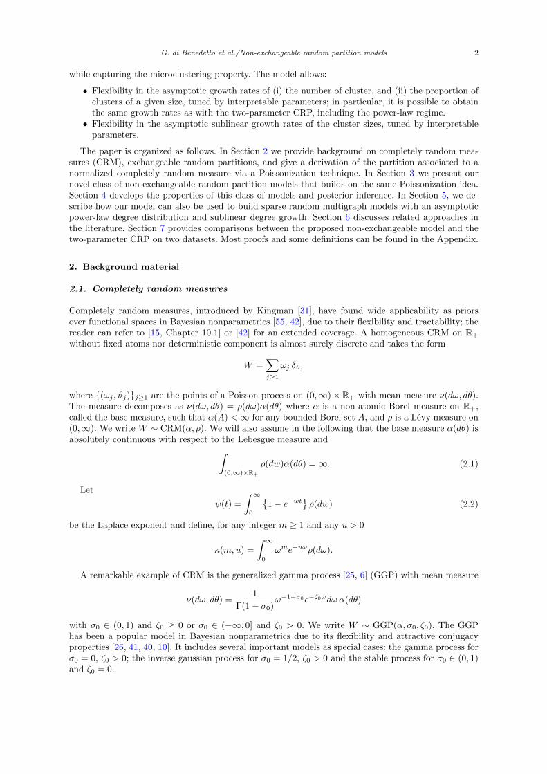
with σ0 ∈ (0, 1) and ζ0 ≥ 0 or σ0 ∈ (−∞, 0] and ζ0 > 0. We write W ∼ GGP(α, σ0, ζ0). The GGPhas been a popular model in Bayesian nonparametrics due to its flexibility and attractive conjugacyproperties [26, 41, 40, 10]. It includes several important models as special cases: the gamma process forσ0 = 0, ζ0 > 0; the inverse gaussian process for σ0 = 1/2, ζ0 > 0 and the stable process for σ0 ∈ (0, 1)and ζ0 = 0.


2.2. Exchangeable random partitions

For an exchangeable partition Π = (Πn)n≥1 of N we have, for every n ≥ 1

Pr(Πn = {An,1, . . . , An,Kn}) = p(|An,1|, . . . , |An,Kn |)

where the sets An,j are considered in order of appearance and p is a symmetric function of its argu-ments called exchangeable partition probability function (EPPF). Therefore, by definition, the orderingin which we observe the data is not taken into account and the only information that affects thedistribution of the random partition is the size of the clusters. For an infinite sequence of randomvariables (θ(1), θ(2), . . .) taking values in R+, let Π(θ(1), θ(2), . . .) be the random partition of N definedby the equivalence relation “i and j are in the same cluster” if and only if θ(i) = θ(j) [50]. By King-man’s representation theorem [32], every exchangeable random partition has the same distribution asΠ(θ(1), θ(2), . . .), where the random variables θ(1), θ(2), . . . are conditionally independent and identicallydistributed from some random probability distribution P.

A popular model for this random probability distribution is a normalized completely random mea-sure [55, 27, 28], defined as P = W/W (R+), where W ∼ CRM(ρ, α) and α(R+) < ∞. This condition,together with the condition (2.1), ensures that 0 < W (R+) < ∞ almost surely, and the model is thusproperly defined.

2.3. Continuous-time embedding of exchangeable random partitions via Poissonization

Let (θ(1), θ(2), . . .) be an infinite sequence of random variables taking values in R+ and Π(θ(1), θ(2), . . .)be the random partition of N defined by the equivalence relation “i and j are in the same cluster” ifand only if θ(i) = θ(j). Let 0 < τ(1) < τ(2) < . . . be an infinite sequence of arrival times. Define thecontinuous-time partition-valued process (Π(t))t≥0 as

Π(t) := ΠN(t) = Π(θ(1), . . . , θ(N(t))), t ≥ 0

where N(t) =∑i 1τ(i)≤t with 1τ≤t = 1 if τ ≤ t and 0 otherwise. (Π(t))t≥0 defines a continuous-time

embedding of the partition Π. Note that we have

Πn = Π(τ(n)) n ≥ 1.

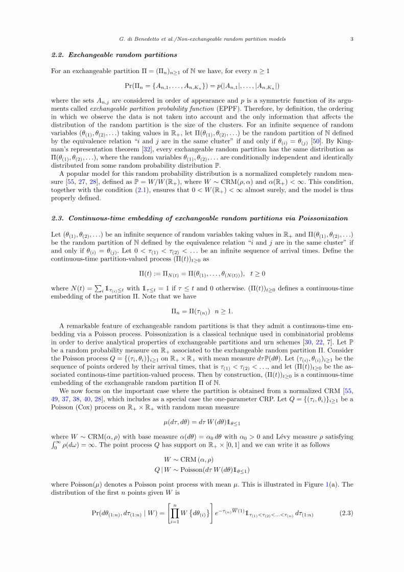
A remarkable feature of exchangeable random partitions is that they admit a continuous-time em-bedding via a Poisson process. Poissonization is a classical technique used in combinatorial problemsin order to derive analytical properties of exchangeable partitions and urn schemes [30, 22, 7]. Let Pbe a random probability measure on R+ associated to the exchangeable random partition Π. Considerthe Poisson process Q = {(τi, θi)}i≥1 on R+×R+ with mean measure dτP(dθ). Let (τ(i), θ(i))i≥1 be thesequence of points ordered by their arrival times, that is τ(1) < τ(2) < . . ., and let (Π(t))t≥0 be the as-sociated continous-time partition-valued process. Then by construction, (Π(t))t≥0 is a continuous-timeembedding of the exchangeable random partition Π of N.

We now focus on the important case where the partition is obtained from a normalized CRM [55,49, 37, 38, 40, 28], which includes as a special case the one-parameter CRP. Let Q = {(τi, θi)}i≥1 be aPoisson (Cox) process on R+ × R+ with random mean measure

µ(dτ, dθ) = dτ W (dθ)1θ≤1

where W ∼ CRM(α, ρ) with base measure α(dθ) = α0 dθ with α0 > 0 and Levy measure ρ satisfying∫∞0ρ(dω) =∞. The point process Q has support on R+ × [0, 1] and we can write it as follows

W ∼ CRM (α, ρ)

Q |W ∼ Poisson(dτ W (dθ)1θ≤1)

where Poisson(µ) denotes a Poisson point process with mean µ. This is illustrated in Figure 1(a). Thedistribution of the first n points given W is

Pr(dθ(1:n), dτ(1:n) |W ) =

[n∏i=1

W{dθ(i)

}]e−τ(n)W (1)1τ(1)<τ(2)<...<τ(n)

dτ(1:n) (2.3)


(a) Poisson embedding of an exchangeable randompartition

(b) Poisson embedding of the non-exchangeable ran-dom partition

Fig 1. (a) The Chinese restaurant process obtained via a Poisson embedding. Points (τi, θi) are drawn from a Poissonpoint process on R+ × [0, 1] with mean measure µ(dτ, dθ) = dτ W (dθ)1θ≤1 where W is a gamma random measure withbase measure α(dθ) = α0dθ and ζ = 1. The red sticks on the θ-axis represent the jumps of the Gamma random measureW . Points on the same horizontal line are in the same cluster. The random partition Π(θ(1), θ(2), . . .) of N induced bythe sequence of points θ(1), θ(2), . . . ordered by their arrival times τ(1) < τ(2) < . . . is the CRP. (b) Non-exchangeablerandom partition model via a Poisson embedding. Points (τi, θi) are drawn from a Poisson point process on R+ × [0, 1]with mean measure µ(dτ, dθ) = dτ W (dθ)1θ≤τ where W is a CRM. The red sticks on the θ-axis represent the jumps ofthe CRM W . Points on the same horizontal line are in the same cluster.

where W (t) =∫ t

0W (dθ) =

∑i≥1 ωi1ϑi≤t. Let us denote by mn,j the number of points in the j-th

cluster after having observed n points, and by (θ∗i )i=1,...,Kn the unique values in (θ(1), . . . , θ(n)), orderedby arrival times. Using the results in [26, Proposition 3.1 page 18], we can obtain the expectation of(2.3) with respect to the CRM W

Pr(dθ(1:n), dτ(1:n)) = e−α0ψ(τ(n))αKn0

Kn∏j=1

κ(mn,j , τ(n)) dθ∗j

1τ(1)<...<τ(n)dτ(1:n).

Integrating over the arrival times τ(i) and the cluster locations θ∗j gives

Pr(Πn) =

∫ ∞0

e−α0ψ(u)αKn0

Kn∏j=1

κ(mn,j , u)

un−1

Γ(n)du,

and one recovers the EPPF of the exchangeable random partition associated to a normalized completelyrandom measure [51, Corollary 6], [28, Proposition 3]. In the gamma process case, κ(m,u) = Γ(m)/(1+u)m and ψ(u) = log(1 + u), yielding

Pr(Πn) =αKn0

Γ(n)

Kn∏j=1

Γ(mn,j)

∫ ∞0

un−1

(1 + u)n+α0du =

αKn0 Γ(α0)

Γ(α0 + n)

Kn∏j=1

Γ(mn,j)

which is the EPPF of the Chinese Restaurant process.

3. Non-exchangeable random partitions

In this section, we build on the Poissonization idea in order to derive a class of non-exchangeable randompartitions. This class is shown to have the microclustering property in the next section. The Cox ProcessQ = {(τi, θi)}i≥1 that defines our non-exchangeable random partition model has the following randommean measure

µ(dτ, dθ) = 1θ≤τW (dθ)dτ (3.1)


therefore the points will lie under the bisector as shown in Figure 1(b). The overall model is thereforedefined as

W ∼ CRM (α, ρ)

Q |W ∼ Poisson(1θ≤τ dτ W (dθ))

The random partition Π = (Πn)n≥1 of N is obtained by considering the points ((τ(i), θ(i)))i≥1 of thepoint process Q ordered by their arrival time, and let Πn = Π(θ(1), . . . , θ(n)) be the partition inducedby the first n points for any n ≥ 1. The random partition model is completely specified by the basemeasure α and the Levy measure ρ.

The crucial difference with the previous construction is the support of the point process. In thecontinuous time version of the CRP, every atom of W in [0, 1] was allowed to be chosen at any time,hence the set of potential cluster labels was constant over time. Now, for every fixed t > 0, all theclusters whose θ are greater than t cannot be chosen before that time, therefore the set of potentialcluster labels increases with t, if for instance the base measure α has unbounded support on R+. Thisproperty intuitively leads to both the non-exchangeability of the random partition induced on N, butalso to the microclustering property.

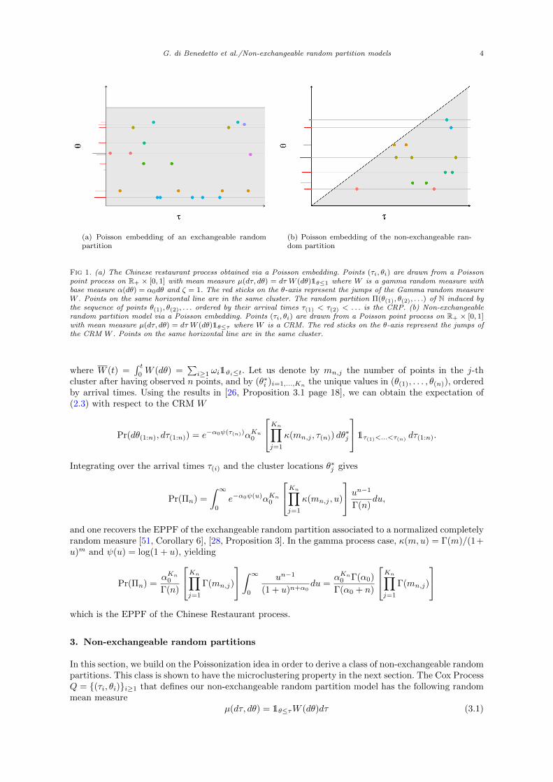
Samples from the process are represented in Figure 2 when W ∼ GGP(α, σ, 1) with base measureα(dθ) = ξθξ−1, for different values of ξ and σ.

0 20 40 60 80 100 120 140

0

20

40

60

80

100

120

140

= 1, = 0.1

0 20 40 60 80 100 120 140

0

20

40

60

80

100

120

140

= 1, = 0.9

0 5 10 15 20 25 30 35 40

0

5

10

15

20

25

30

35

40

= 2, = 0.5

0 1 2 3 4 5 6 7 8

0

1

2

3

4

5

6

7

8

= 4, = 0.5

Fig 2. Samples from the Cox Process Q where W ∼ GGP (α, σ, 1) with base measure α(dθ) = ξ θξ−1 dθ, for differentvalues of σ and ξ.

Proposition 1. Let W be a homogeneous CRM(α, ρ) and a point process Q = {(τi, θi)}i≥1 on R2+ with

mean measure µ(dτ dθ) = 1θ≤τdτ W (dθ). Let ((τ(i), θ(i)))i≥1 be the sequence of points ordered in time,that is such that τ(1) < τ(2) < . . .. For any n ≥ 1,

Pr(dθ(1:n), dτ(1:n)) =

Kn∏j=1

κ(mn,j , τ(n) − θ∗j )α(dθ∗j )

e− ∫ τ(n)0 ψ(τ(n)−θ)α(dθ)

×

[n∏i=1

1θ(i)≤τ(i)

]1τ(1)<τ(2)<...<τ(n)

dτ(1:n) (3.2)


where θ∗j , j = 1, . . . ,Kn, are the unique values of (θ(1), . . . , θ(n)), and mn,j their multiplicities.

Proof. The derivation is similar to the derivation for the exchangeable case described in the previoussection. Given W , the set of points (τi)i≥1 is an inhomogeneous Poisson point process on R+ with rateW (t), hence

Pr(dτ(1:n) |W ) = e−∫ τ(n)0 W (t)dt

[n∏i=1

W (τ(i))

]1τ(1)<...<τ(n)

dτ(1:n).

Given the n time variables, the θ(i)’s are distributed as follows

Pr(dθ(1:n) | τ(1:n),W ) =

n∏i=1

W (dθ(i))

W (τ(i))1θ(i)<τ(i) .

It follows that

Pr(dθ(1:n), dτ(1:n) |W ) =

[n∏i=1

W (dθ(i))1θ(i)≤τ(i)

]e−

∫ τ(n)0 W (t)dt1τ(1)<...<τ(n)

dτ(1:n) (3.3)

where∫ τ(n)

0W (t)dt =

∑j ωi(τ(n) − ϑj)+ = W (gτ(n)

) with gt(x) = (t − x)+ = max(0, t − x). Using[26, Proposition 3.1], we can integrate over W to obtain the final result.

Integrating Equation (3.2) over the cluster allocations (θ∗j )j=1,...,Kn and the arrival times τ(1:n), wewould obtain the distribution of the random partition Πn. To the best of our knowledge, there is howeverno analytical expression for this distribution. We can nonetheless simulate random partitions by usingthe cluster allocations and arrival times as latent variables. In particular, for the generalized gammaprocess, we have the following result.

Proposition 2. Let W ∼ GGP (α, σ0, ζ0), and Q = {(τi, θi)}i≥1 be the points of a Cox process withmean measure µ(dτ, dθ) = 1θ≤τW (dθ)dτ . Then the predictive distribution of τ(n) has density

p(τ(n) | (θ(i), τ(i))i=1,...,n−1) ∝

Kn−1∏j=1

1

(τ(n) − θ∗j + ζ0)mn−1,j−σ0

e− ∫ τ(n)0 ψ(τ(n)−θ)α(dθ)

×

(Kn−1∑j=1

mn−1,j − σ0

τ(n) − θ∗j + ζ0+

∫ τ(n)

0

α(θ)

(τ(n) − θ + ζ0)1−σ0dθ

)1τ(n)>τ(n−1)

where ψ(t) = log(1+t/ζ0) for σ0 = 0, while ψ(t) = ((t+ ζ0)σ0 − ζσ00 ) /σ0 for σ0 ∈ (0, 1). The conditional

distribution for θ(n) is a convex combination of a discrete distribution and a diffuse one,

Pr(θ(n) ∈ dθ | (θ(i), τ(i))i=1,...,n−1, τ(n)) ∝ Hτ(n)(dθ) +

Kn−1∑i=1

mn−1,i − σ0

τ(n) − θ∗i + ζ0δθ∗i (dθ)

where Ht is a diffuse distribution defined as Ht(A) =∫A

1θ≤t(t−θ+ζ0)1−σ0

α(dθ) for every Borel set A ⊂ R+.

For example, if W is a gamma process (σ0 = 0) and α(dθ) = dθ, we obtain

p(τ(n) | (θ(i), τ(i))i=1,...,n−1) ∝

Kn−1∏j=1

1

(τ(n) − θ∗j + ζ0)mn−1,j

e−τ(n)

(1 +

τ(n)

ξ0

)−τ(n)−ξ0

×

(Kn−1∑j=1

mn−1,j

τ(n) − θ∗j + ζ0+ log(1 + τ(n)/ζ0)

)1τ(n)>τ(n−1)

,

and {Pr(θ(n) = θ∗j | (θ(i), τ(i))i=1,...,n−1, τ(n)) = Cn

mn−1,j

τ(n)−θ∗j+ζ0for j = 1, . . . ,Kn−1

Pr(θ(n) is new | (θ(i), τ(i))i=1,...,n−1, τ(n)) = Cn log(1 + τ(n)/ζ0)

where Cn is the appropriate normalizing constant.


4. Properties and inference

4.1. Asymptotic properties

In this section, denote Xt ∼ Yt, Xt = o(Yt) and Xt = O(Yt) respectively for Xt/Yt → 1, Xt/Yt → 0and lim suptXt/Yt < ∞. The notation Xt � Yt means both Xt = O(Yt) and Yt = O(Xt) hold. WhenXt and/or Yt are random variables the asymptotic relation is meant to hold almost surely.

The properties we are most interested in are the asymptotic behaviour of the cluster sizes mn,j , ofthe number Kn of clusters and the number Kn,r of clusters of size r in the random partition. We showin this section that our non-exchangeable model allows for a sublinear growth of the clusters’ sizes whileretaining desirable properties for the other quantities. Let us list the assumptions on the CRM W toderive the asymptotic results.

(A1) W has finite first two moments, that is

κ(1, 0) =

∫ ∞0

ωρ(dω) <∞ and κ(2, 0) =

∫ ∞0

ω2ρ(dω) <∞.

(A2) The Levy tail intensity ρ(x) =∫∞xρ(dω) is a regularly varying function at 0, that is

ρ(x) ∼ ` (1/x)x−σ

as x→ 0+, where ` is a slowly varying function at infinity and σ ∈ [0, 1].

(A3) The improper cumulative distribution α(t) =∫ t

0α(dx) of the base measure α is a regularly varying

function at infinity, that isα(t) ∼ L(t) tξ

as t → ∞, where ξ > 0 and L is a slowly varying function. Assume additionally that the basemeasure α is dominated by the Lebesgue measure, and admits a continuous and monotone densitydenoted α(θ).

The moment assumption (A1) excludes the stable process that has infinite first moment. (A2) controls,through the parameter σ, the power-law behaviour of the proportion of clusters of a given size, whilecondition (A3) is used to prove the microclustering property and control the sublinear rate of theclusters’ size. It is worth noting that the last condition is very mild and allows to pick the density ofthe base measure from a very large class of functions. Assumptions (A1-A2) are satistied for the GGPwith parameters σ0 ∈ (−∞, 1) and ζ0 > 0. In this case, we have σ = max(σ0, 0) and `(t) ∝ log t forσ = 0 and `(t) is constant otherwise.

Recall thatN(t) =

∑i≥1

1τi≤t

denotes the number of points of Q such that τi ≤ t. For each atom ϑj , j ≥ 1, of the CRM W , let

Xj(t) =∑i≥1

1τi≤t1θi=ϑj .

For j ≥ 1, let

Mj(t) =∑i≥1

1τi≤t1θi=θ∗j

the size of cluster j, ordered by appearance, at time t. Note that N(τ(n)) = n and Mj(τ(n)) = mn,j .

Proposition 3. Let W =∑j≥1 ωiδϑj be a CRM with mean measure α(dθ)ρ(dω) satisfying Assumptions

(A1-A3). Let {(τi, θi)}i≥1 be a Poisson point process with mean measure µ(dτ dθ) = 1θ≤τdτ W (dθ).We have, almost surely as t tends to infinity,

N(t) ∼ κ(1, 0)

ξ + 1tξ+1L(t)

and, for j ≥ 1

Xj(t) ∼W ({ϑj})tMj(t) ∼W ({θ∗j })t.


Proposition 3 implies the microclustering property for the random partition Πn: almost surely,Mj(t)/N(t)→ 0 as t→∞, hence mn,j/n→ 0 as n→∞. In the following corollary, which follows fromproperties of inverse of regularly varying functions [3, Proposition 1.5.15] or [22, Lemma 22], we obtainexact rates of growth for the cluster sizes.

Corollary 4 (Microclustering property). We have

t ∼(ξ + 1

κ(1, 0)

)1/(ξ+1)

L∗ξ+1(N(t))N(t)1/(ξ+1) (4.1)

almost surely as t → ∞, where L∗ξ+1 is a slowly varying function defined in equation (B.1) in theAppendix. It follows that the cluster sizes mn,j = Mj(τ(n)) verify, for any j ≥ 1,

mn,j ∼W ({θ∗j })(ξ + 1

κ(1, 0)

)1/(ξ+1)

L∗ξ+1(n)n1/(ξ+1)

almost surely as n tends to infinity. For j = 1, the distribution of ω∗1 = W ({θ∗1}) is given by

Pr(dω∗1) = ω∗1ρ(dω∗1)

∫ ∞0

∫ τ

0

e−ω∗1 (τ−θ)e−

∫ t0ψ(τ−u)α(du)α(dθ)dτ.

Note that the growth rate of the cluster sizes only depends on the parameters ξ and L of the basemeasure α, and not on the properties of the Levy measure ρ. For example, taking α(t) = γtξ, withξ, γ > 0, we have L(t) = γ and mn,j � n1/(ξ+1) and the cluster sizes grow at a rate of na where0 < a < 1.

We now provide results on the asymptotic rates of the number of clusters and number of clustersof a given size, showing that we can have the same range of behaviour as for exchangeable randompartitions. Let

K(t) =∑j≥1

1Xj(t)>0

be the number of different clusters in Π(t) at time t and

Kr(t) =∑j≥1

1Xj(t)=r

the number of clusters of size r at time t.

Proposition 5. Let W =∑j≥1 ωiδϑj be a CRM with mean measure α(dθ)ρ(dω) satisfying Assumptions

(A1-A3). Define {`σ(t) = Γ(1− σ)`(t) ifσ ∈ [0, 1)`1(t) =

∫∞ty−1`(y)dy ifσ = 1.

Let {(τi, θi)}i≥1 be a Poisson point process with mean measure µ(dτ dθ) = 1θ≤τdτ W (dθ). We have,almost surely at t tends to infinity,

K(t) ∼ Γ(σ + 1)Γ(ξ + 1)

Γ(σ + ξ + 1)L(t)`σ(t) tσ+ξ.

For r ≥ 1, if σ = 0 then Kr(t) = o(K(t)), if σ ∈ (0, 1),

Kr(t) ∼σΓ(r − σ)

r!Γ(1− σ)K(t) .

If σ = 1, K1(t) ∼ K(t) and Kr(t) = o(K(t)) for all r ≥ 2.

By noting that Kn = K(τ(n)) and Kn,r = Kr(τ(n)), we can combine the results of Proposition 5 andEquation (4.1) to obtain asymptotic expressions for the number Kn of clusters and the number Kn,j

of clusters of size j in Πn.

Corollary 6. We have, almost surely as n tends to infinity,

Kn ∼ ˜(n)n(σ+ξ)/(ξ+1)


100 101 102 103

r

10 6

10 5

10 4

10 3

10 2

10 1

100

Kn, r

Kn

= 0.1= 0.5= 0.9

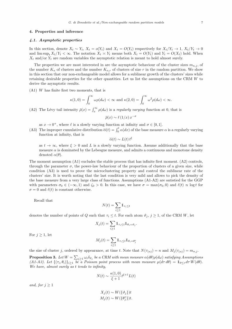
Fig 3. Log-log plot of the proportions of clusters of given size for the GGP with α(dθ) = dθ, ζ0 = 1, σ = 0.1, 0.5, 0.9 andsample size 10000.

where ˜ is a slowly varying function defined in equation (B.2) in the Appendix.For r ≥ 1, if σ = 0 then Kn,r = o(Kn); if σ ∈ (0, 1),

Kn,r

Kn→ σΓ(r − σ)

r!Γ(1− σ).

This corresponds to a power-law behaviour for the proportion of clusters of size r, as

σΓ(r − σ)

r!Γ(1− σ)� 1

j1+σ

for large j. If σ = 1, Kn,1 ∼ Kn and Kn,r = o(Kn) for all r ≥ 2. In this case, the proportion of clustersof size 1 tends to one almost surely.

Example 7. If W ∼ GGP(α, σ, 1) with σ ∈ (0, 1) and base measure α(dθ) = γξθξ−1dθ with ξ, γ > 0we have `(t) = 1

σ Γ(1−σ) and L(t) = γ, therefore

Kn ∼Γ(σ + 1)Γ(ξ + 1)

σΓ(σ + ξ + 1)(ξ + 1)

σ+ξ1+ξ γ1−σ+ξ1+ξ n

σ+ξ1+ξ

and for all r ≥ 1

Kn,r

Kn→ σΓ(r − σ)

r!Γ(1− σ)

almost surely as n tends to infinity. This power-law behavior is illustrated on Figure 3.

It is worth noting that although the asymptotic behaviour of the number of clusters and the numberof clusters of a given size depend also on the base measure α, the power-law exponent in the proportionof clusters of a given size is solely tuned by the Levy measure ρ through the parameter σ.

4.2. Inference

4.2.1. Posterior characterization

Assuming we observe the first n time-ordered points (τ(i), θ(i))i=1,...,n from the Cox process Q, we wantto characterize the conditional distribution of the CRM W given the time-ordered observations. Thefollowing posterior characterization follows from [26, Proposition 3.1 page 18].

Proposition 8. Given the first n time-ordered observations (τ(i), θ(i))i=1,...,n from the Cox process Q,with unique cluster labels θ∗1 , . . . , θ

∗Kn

, the conditional distribution of the CRM W is given by

W ′ +

Kn∑j=1

ω∗j δθ∗j


where the random positive weights (ω∗1 , . . . , ω∗Kn

) are independent of the random measure W ′. W ′ is an

inhomogeneous CRM with mean measure ν′(dω, dθ) = e−ω(τ(n)−θ)+ρ(dω)α(dθ). The masses of the fixedatoms are conditionally independent with density

p(ω∗j | rest) ∝ ρ(dω∗j )ω∗mn,jj e−ω

∗j (τ(n)−θ∗j ).

In particular, when W is a generalized gamma process the masses are conditionally gamma distributed

ω∗j | rest ∼ Gamma(mn,j − σ0, ζ0 + τ(n) − θ∗j ).

4.2.2. Parameter estimation and prediction

We consider the CRM with base measure α(dθ) = ξ θξ−1dθ and generalized gamma Levy measure withparameters σ0 and ζ0. The set of parameters is therefore η = (ξ, σ0, ζ0). Having observed a partition Πn,we aim at estimating the parameters η and predict Πn+m for m ≥ 1. The marginal likelihood Pr(Πn|η)is however intractable. We use a sequential Monte Carlo algorithm [18, 47] with target distributionPr(dθ(1:n), dτ(1:n)|Πn, η) in order to get unbiased estimators of the marginal likelihoods Pr(Πn|η) for agrid of values of η, and compute the maximum likelihood estimate η. The proposal distribution for thearrival times τ(n) is a truncated normal on [τ(n−1),∞), while the proposal for the cluster location of anew cluster is uniform on [0, τ(n)]. We also use a sequential Monte Carlo algorithm in order to samplefrom the predictive Pr(Πn+m|Πn, η) using Proposition 8.

5. Random partitions and random multigraphs

The non-exchangeable random partition model proposed can be used to derive models for randommultigraphs, see [5]. Recall that Πn = (An,1, . . . , An,Kn), where the blocks are sorted in order ofappearance. For each i = 1, 2, . . ., let ci be the index of the cluster to which item i belongs, that isi ∈ An,ci for all n ≥ i. An undirected multigraph G = Φ(Π), possibly with self-loops and with acountably infinite number of edges, is derived from the random partition Π by

G = ((c1, c2), (c3, c4), . . .)

where each pair (c2n−1, c2n) represents an undirected edge between the vertex c2n−1 and the vertex c2n.The set of vertices is either {1, . . . ,K} if the partition has a finite number of blocks, or the set N. LetGn be the restriction of G to the first n edges that is, to the first 2n items of Π. Then K2n, the numberof clusters in Π2n, is also the number of vertices of Gn, m2n,j is the degree of vertex j, j = 1, . . . ,K2n

and K2n,j/K2n is the proportion of vertices of degree j.The multigraphs G obtained by transformation of an exchangeable random partition form a subclass

of the edge-exchangeable graphs [14, 8]. This subclass is called rank one edge-exchangeable graphsby Janson [29]. Of particular interest is the so-called Hollywood model [14], obtained from a two-parameter CRP random partition. In this case, inherited from the properties of the associated randompartition [52], one can obtain sparse multigraphs with power-law degree distribution. A consequence ofthe exchangeability assumption is the fact that the degree sequence grows linearly with the number ofedges: for any vertex j, its degree m2n,j � n almost surely as the number of edges n tends to infinity.As shown in the following corollary of the results of Section 4, our construction allows to obtain sparsemultigraphs with power-law degree distribution and sublinear growth rate for degree sequences.

Corollary 9. Let Π be a non-exchangeable partition with parameters α and ρ verifying assumptions(A1-A3). Let G = Φ(Π) the associated random multigraph. For a subgraph Gn corresponding to thefirst n edges, let K2n be the number of vertices, m2n,j the degree of vertex j and K2n,r the number ofvertices of degree r ≥ 1. Then, almost surely as the number of edges n tends to infinity

m2n,j � L∗ξ+1(n)n1/(1+ξ), j ≥ 1

K2n ∼ ˜(n)(2n)(σ+ξ)/(1+σ)

K2n,r

K2n→ σΓ(r − σ)

r!Γ(1− σ), r ≥ 1

where the slowly varying functions L∗ξ+1 and ˜ are defined in Equations (B.1) and (B.2).


0.0 0.2 0.4 0.6 0.8 1.0

σ

28000

27500

27000

26500

26000

25500

25000

24500

24000

23500

Loglik

elih

ood

MLξ= 1

ξ= 2

ξ= 3

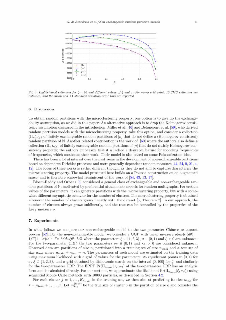
Fig 4. Loglikelihood estimates for ζ = 10 and different values of ξ and σ. For every grid point, 10 SMC estimates areobtained, and the mean and ±1 standard deviation error bars are reported.

6. Discussion

To obtain random partitions with the microclustering property, one option is to give up the exchange-ability assumption, as we did in this paper. An alternative approach is to drop the Kolmogorov consis-tency assumption discussed in the introduction. Miller et al. [46] and Betancourt et al. [59], who derivedrandom partition models with the microclustering property, take this option, and consider a collection(Πn)n≥1 of finitely exchangeable random partitions of [n] that do not define a (Kolmogorov-consistent)random partition of N. Another related contribution is the work of [60] where the authors also define acollection (Πn)n≥1 of finitely exchangeable random partitions of [n] that do not satisfy Kolmogorov con-sistency property; the authors emphasize that it is indeed a desirable feature for modeling frequenciesof frequencies, which motivates their work. Their model is also based on some Poissonization idea.

There has been a lot of interest over the past years in the development of non-exchangeable partitionsbased on dependent Dirichlet processes and more generally dependent random measures [44, 24, 9, 21, 4,12]. The focus of these works is rather different though, as they do not aim to capture/characterize themicroclustering property. The model presented here builds on a Poisson construction on an augmentedspace, and is therefore somewhat reminiscent of the work of [54, 43, 13, 17].

Bloem-Reddy and Orbanz [5] considered a general class of exchangeable and non-exchangeable ran-dom partitions of N, motivated by preferential attachments models for random multigraphs. For certainvalues of the parameters, it can generate partitions with the microclustering property, but with a some-what different asymptotic behavior for the number of clusters. The microclustering property is obtainedwhenever the number of clusters grows linearly with the dataset [5, Theorem 7]. In our approach, thenumber of clusters always grows sublinearly, and the rate can be controlled by the properties of theLevy measure ρ.

7. Experiments

In what follows we compare our non-exchangeable model to the two-parameter Chinese restaurantprocess [52]. For the non-exchangeable model, we consider a GGP with mean measure ρ(dω)α(dθ) =1/Γ(1− σ)ω−1−σe−ζωdωξθξ−1dθ where the parameters ξ ∈ {1, 2, 3}, σ ∈ [0, 1) and ζ > 0 are unknown.For the two-parameter CRP, the two parameters σ2 ∈ [0, 1) and κ2 > 0 are considered unknown.Observed data are partitions of size n, partitioned into a training set of size ntrain and a test set ofsize ntest where ntrain + ntest = n. The parameters of each model are estimated on the training datausing maximum likelihood with a grid of values for the parameters: 25 equidistant points in [0, 1) forσ, ξ ∈ {1, 2, 3}, and a grid obtained by dichotomic search on the interval [0, 100] for ζ, and similarlyfor the two-parameter CRP. The EPPF Pr(Πntrain

|σ2, κ2) of the two-parameter CRP has an analyticform and is calculated directly. For our method, we approximate the likelihood Pr(Πntrain

|ξ, σ, ζ) usingsequential Monte Carlo methods with 10000 particles, as described in Section 4.2.

For each cluster j = 1, . . . ,Kntrain in the training set, we then aim at predicting its size mk,j for

k = ntrain + 1, . . . , n. Let m(true)k,j be the true size of cluster j in the partition of size k and consider the


5000 10000 15000sample size

0

20

40

60

80

100

size

of

the c

lust

ers

(a) Synthetic

5000 10000 15000sample size

0

20

40

60

80

100

size

of

the c

lust

ers

(b) Amazon

5000 10000 15000sample size

0

100

200

300

size

of

the c

lust

ers

(c) Math Overflow

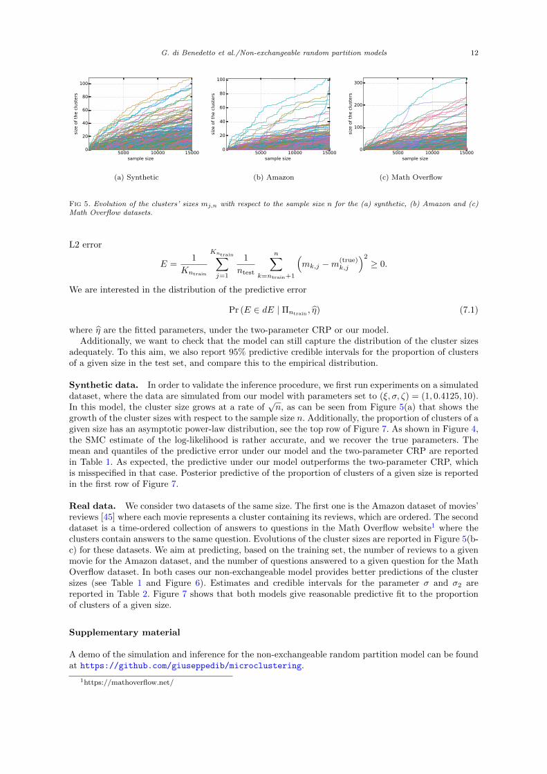
Fig 5. Evolution of the clusters’ sizes mj,n with respect to the sample size n for the (a) synthetic, (b) Amazon and (c)Math Overflow datasets.

L2 error

E =1

Kntrain

Kntrain∑j=1

1

ntest

n∑k=ntrain+1

(mk,j −m(true)

k,j

)2

≥ 0.

We are interested in the distribution of the predictive error

Pr (E ∈ dE | Πntrain, η) (7.1)

where η are the fitted parameters, under the two-parameter CRP or our model.Additionally, we want to check that the model can still capture the distribution of the cluster sizes

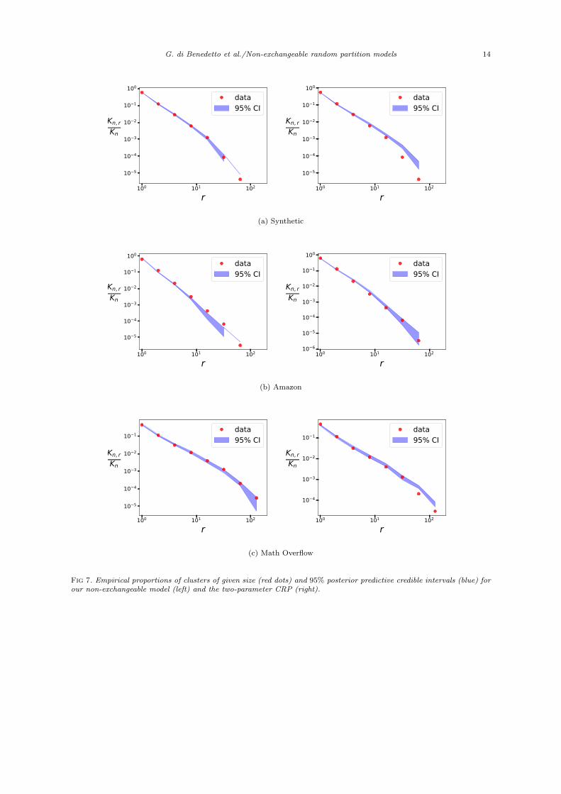
adequately. To this aim, we also report 95% predictive credible intervals for the proportion of clustersof a given size in the test set, and compare this to the empirical distribution.

Synthetic data. In order to validate the inference procedure, we first run experiments on a simulateddataset, where the data are simulated from our model with parameters set to (ξ, σ, ζ) = (1, 0.4125, 10).In this model, the cluster size grows at a rate of

√n, as can be seen from Figure 5(a) that shows the

growth of the cluster sizes with respect to the sample size n. Additionally, the proportion of clusters of agiven size has an asymptotic power-law distribution, see the top row of Figure 7. As shown in Figure 4,the SMC estimate of the log-likelihood is rather accurate, and we recover the true parameters. Themean and quantiles of the predictive error under our model and the two-parameter CRP are reportedin Table 1. As expected, the predictive under our model outperforms the two-parameter CRP, whichis misspecified in that case. Posterior predictive of the proportion of clusters of a given size is reportedin the first row of Figure 7.

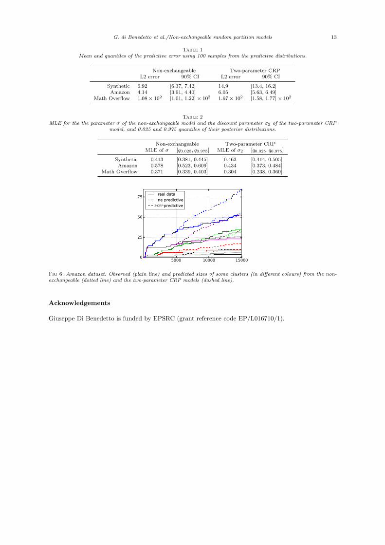
Real data. We consider two datasets of the same size. The first one is the Amazon dataset of movies’reviews [45] where each movie represents a cluster containing its reviews, which are ordered. The seconddataset is a time-ordered collection of answers to questions in the Math Overflow website1 where theclusters contain answers to the same question. Evolutions of the cluster sizes are reported in Figure 5(b-c) for these datasets. We aim at predicting, based on the training set, the number of reviews to a givenmovie for the Amazon dataset, and the number of questions answered to a given question for the MathOverflow dataset. In both cases our non-exchangeable model provides better predictions of the clustersizes (see Table 1 and Figure 6). Estimates and credible intervals for the parameter σ and σ2 arereported in Table 2. Figure 7 shows that both models give reasonable predictive fit to the proportionof clusters of a given size.

Supplementary material

A demo of the simulation and inference for the non-exchangeable random partition model can be foundat https://github.com/giuseppedib/microclustering.

1https://mathoverflow.net/

https://github.com/giuseppedib/microclustering


Table 1Mean and quantiles of the predictive error using 100 samples from the predictive distributions.

Non-exchangeable Two-parameter CRPL2 error 90% CI L2 error 90% CI

Synthetic 6.92 [6.37, 7.42] 14.9 [13.4, 16.2]Amazon 4.14 [3.91, 4.40] 6.05 [5.63, 6.49]

Math Overflow 1.08 × 102 [1.01, 1.22] × 102 1.67 × 102 [1.58, 1.77] × 102

Table 2MLE for the the parameter σ of the non-exchangeable model and the discount parameter σ2 of the two-parameter CRP

model, and 0.025 and 0.975 quantiles of their posterior distributions.

Non-exchangeable Two-parameter CRPMLE of σ [q0.025, q0.975] MLE of σ2 [q0.025, q0.975]

Synthetic 0.413 [0.381, 0.445] 0.463 [0.414, 0.505]Amazon 0.578 [0.523, 0.609] 0.434 [0.373, 0.484]

Math Overflow 0.371 [0.339, 0.403] 0.304 [0.238, 0.360]

5000 10000 150000

25

50

75real data

ne predictive

py predictive2-CRP

Fig 6. Amazon dataset. Observed (plain line) and predicted sizes of some clusters (in different colours) from the non-exchangeable (dotted line) and the two-parameter CRP models (dashed line).

Acknowledgements

Giuseppe Di Benedetto is funded by EPSRC (grant reference code EP/L016710/1).


100 101 102

r

10 5

10 4

10 3

10 2

10 1

100

Kn, r

Kn

data95% CI

100 101 102

r

10 5

10 4

10 3

10 2

10 1

100

Kn, r

Kn

data95% CI

(a) Synthetic

100 101 102

r

10 5

10 4

10 3

10 2

10 1

100

Kn, r

Kn

data95% CI

100 101 102

r10 6

10 5

10 4

10 3

10 2

10 1

100

Kn, r

Kn

data95% CI

(b) Amazon

100 101 102

r

10 5

10 4

10 3

10 2

10 1

Kn, r

Kn

data95% CI

100 101 102

r

10 4

10 3

10 2

10 1

Kn, r

Kn

data95% CI

(c) Math Overflow

Fig 7. Empirical proportions of clusters of given size (red dots) and 95% posterior predictive credible intervals (blue) forour non-exchangeable model (left) and the two-parameter CRP (right).


Appendix A: Proof of the main theorems

Proof of proposition 2. From Eq. (3.2), the joint distribution of ((θ(i), τ(i))i=1,...,n) is given by

Pr(dθ(1:n),dτ(1:n)) =

{Kn−1∑i=1

Kn−1∏j=1j 6=i

κ(mn−1,j , τ(n) − θ∗j )α(θ∗j )

κ(mn−1,i + 1, τ(n) − θ∗i )α(θ∗i ) δθ∗i (dθ(n))

+

Kn−1∏j=1

κ(mn−1,j , τ(n) − θ∗j )α(θ∗j )

κ(1, τ(n) − θ∗n)α(θ∗n) dθ(n)

}

× e−∫ τ(n)0 ψ(τ(n)−θ)α(dθ)

[n∏i=1

1θ(i)<τ(i)

]1τ(1)<τ(2)<...<τ(n)

dθ(1:n−1)dτ(1:n).

Integrating over θ(n), we obtain

Pr(dθ(1:n−1),dτ(1:n)) =

{Kn−1∑i=1

Kn−1∏j=1j 6=i

κ(mn−1,j , τ(n) − θ∗j )α(θ∗j )

κ(mn−1,i + 1, τ(n) − θ∗i )α(θ∗i )

+

Kn−1∏j=1

κ(mn−1,j , τ(n) − θ∗j )α(θ∗j )

∫ τ(n)

0

κ(1, τ(n) − θ(n))α(θ(n)) dθ(n)

}

e−∫ τ(n)0 ψ(τ(n)−θ)α(dθ)

[n−1∏i=1

1θ(i)<τ(i)

]1τ(1)<τ(2)<...<τ(n)

dθ(1:n−1)dτ(1:n).

In the Generalised Gamma Process case we have

κ(m,u) =1

Γ(1− σ)

Γ(m− σ)

(ζ + u)m−σ.

Therefore κ(m+ 1, u) = κ(m,u)m−σζ+u and

Kn−1∑i=1

Kn−1∏j=1j 6=i

κ(mn−1,j , τ(n) − θ∗j )α(θ∗j )

κ(mn−1,i + 1, τ(n) − θ∗i )α(θ∗i )

=

Kn−1∏j=1

κ(mn−1,j , τ(n) − θ∗j )α(θ∗j )

Kn−1∑i=1

mn−1,i − στ(n) − θ∗i + ζ

hence

Pr(dθ(1:n−1),dτ(1:n)) =1

Γ(1− σ)Kn−1

Kn−1∏j=1

Γ(mn−1,j − σ)α(θ∗j )

(τ(n) − θ∗j + ζ)mn−1,j−σ

×

(Kn−1∑j=1

mn−1,j − στ(n) − θ∗j + ζ

+

∫ τ(n)

0

α(θ)

(τ(n) − θ + ζ)1−σ dθ

)

× e−∫ τ(n)0 ψ(τ(n)−θ)α(dθ)

[n−1∏i=1

1θ(i)<τ(i)

]1τ(1)<...<τ(n)

dθ(1:n−1)dτ(1:n)

from which we obtain the results of the theorem.


Proof of proposition 3. GivenW ,N(t) is a non-homogeneous Poisson process with rateW (t) =∑j≥1 ωj1ϑj≤t.

Hence, using Fubini’s and Campbell’s theorems,

E[N(t)] = E[∫ t

0

W (x)dx

]= α(t)κ(1, 0)

where α(t) =∫ t

0α(t). Similarly,

var(N(t)) = var(E[N(t) |W ]) + E[var(N(t) |W )] = var(W (t)) + E[W (t)]

= κ(2, 0)

∫ t

0

(t− θ)2α(dθ) + κ(1, 0)α(t)

= κ(2, 0)

∫ t

0

α(x)dx+ κ(1, 0)α(t)

Using Karamata’s theorem [3, Proposition 1.5.8] and Assumption (A3), we obtain that

E[N(t)] ∼ κ(0, 1)

ξ + 1tξ+1L(t) and var(N(t)) ∼ κ(2, 0)

(ξ + 1)(ξ + 2)tξ+2L(t).

Therefore, for any 0 < a < ξ we have var(N(t)) = O(t−aE[N(t)2]). Using [11, Lemma B.1], we concludethat, almost surely as t tends to infinity

N(t) ∼ E[N(t)] ∼ κ(1, 0)

ξ + 1tξ+1L(ξ).

Conditional on W , Xj(t) is a non-homogeneous Poisson process with rate ωj1ϑi>t hence

Xj(t) ∼ ωjt

almost surely as t tends to infinity. It follows similarly that Mj(t), the size, at time t, of the jth clusterto appear, satisfies

Mj(t) ∼ ω∗j t

where ω∗j = W ({θ∗j }). Additionally, Propositions 1 and 8 imply that

Pr(dω∗1 , dθ(1), dτ(1)) = ω∗1e−ω∗

1 (τ(1)−θ(1))ρ(dω∗1)α(dθ(1))e−

∫ τ(1)0 ψ(τ(1)−θ)α(dθ)1θ(1)<τ(1) dτ(1).

It follows

Pr(dω∗1) = ω∗1ρ(dω∗1)

∫ ∞0

∫ τ

0

e−ω∗1 (τ−θ)e−

∫ t0ψ(τ−u)α(du)α(dθ)dτ.

Proof of proposition 5. Observe that Pr(Xj(t) > 0 | W ) = 1 − e−ωj(t−θj)+ . By the marking theo-rem [34, Chapter 5], for each t, {(ωj , ϑj) | j ≥ 1, Xj(t) > 0} is a Poisson point process with meanmeasure ρ(dω)α(dθ)(1− e−ω(t−θ)+). It follows that

E[K(t)] = var[K(t)] =

∫ ∞0

∫ t

0

(1− e−(t−θ)ω

)α(dθ)ρ(dω) =

∫ t

0

ψ(t− θ)α(dθ).

Similarly to [22, Proposition 2], it follows from the monotonicity of K(t) and the Borel-Cantelli lemmathat K(t) ∼ E[K(t)] almost surely as t→∞. Using the Tauberian theorems [20, Chapter XIII, Section5] recalled in Lemma 11, Lemma 12 and α(t) ∼ ξtξ−1L(t), we obtain

E[K(t)] ∼ Γ(σ + 1)Γ(ξ + 1)

Γ(σ + ξ + 1)L(t)`σ(t) tσ+ξ

as t tends to infinity.


We proceed similarly for Kr(t). For each t > 0 and r ≥ 1, {(ωj , ϑj) | j ≥ 1, Xj(t) = r} is a Poisson

point process with mean measure ρ(dω)α(dθ)ωr(t−θ)r+

r! e−ω(t−θ)+ . It follows that

E[Kr(t)] = var[Kr(t)]

=

∫ t

0

∫ ∞0

(t− θ)r

r!ωre−(t−θ)ωρ(dω)α(dθ)

=

∫ t

0

(t− θ)r

r!κ(r, t− θ)α(dθ).

Using Lemma 11 and 12, we obtain: if σ = 0, E[Kr(t)] = o(L(t)`(t))tσ+ξ; if σ ∈ (0, 1),

E[Kr(t)] ∼σΓ(r − σ)

r!Γ(1− σ)

Γ(σ + 1)Γ(ξ + 1)

Γ(σ + ξ + 1)L(t)`σ(t) tσ+ξ.

If σ = 1, E[K1(t)] ∼ Γ(σ+1)Γ(ξ+1)Γ(σ+ξ+1) L(t)`σ(t) tσ+ξ and E[Kr(t)] = o(L(t)`(t))tσ+ξ for all r ≥ 2. For the

almost sure result, we proceed as for K(t) [22], using the monotonicity of∑r≥sKr(t), the equality

var[∑

r≥sKr(t)]

= E[∑

r≥sKr(t)]

and the fact that E[Kr(t)] � K(t) for σ ∈ (0, 1), E[Kr(t)] =

o(K(t)) for σ = 0 and E[K1(t)] ∼ K(t) for σ = 1.

Appendix B: Background on regular variation and technical lemma

We recall the following definitions which can be found in [3] and [56].

Definition 10 (Regularly varying function). A measurable function f : R+ → R+ is regularly varyingat ∞ with index ξ ∈ R if for every x > 0

limt→∞

f(tx)

f(t)= xξ.

If ξ = 0 we say that the function is slowly varying. An important property of the regularly varyingfunction is that they can be written as f(x) = `(x)xξ where ξ is the exponent of variation and ` is aslowly varying function.

Let L# be the de Brujin conjugate [3] of a slowly varying function L. Regularly varying functionsf(x) = L(x)xξ of index ξ > 0 admit asymptotic inverse g(x) = L∗ξ(x)x1/ξ which are regularly varying

of index ξ−1 (see [3, Proposition 1.5.15] or [22, Lemma 22]) with slowly varying part

L∗ξ(x) = {L1/ξ(x1/ξ)}#. (B.1)

Note that if L(t) = c, then L∗ξ(t) = c1/ξ. From Equation (4.1) and Proposition 5, it follows that theslowly varying function appearing in Corollary 6 is

˜(n) =Γ(σ + 1)Γ(ξ + 1)

Γ(σ + ξ + 1)

(ξ + 1

κ(1, 0)

)(σ+ξ)/(ξ+1)

L∗ξ+1(n)σ+ξ

× L

{(ξ + 1

κ(1, 0)

)1/(ξ+1)

n1/(ξ+1)L∗ξ+1(n)

}`σ

{(ξ + 1

κ(1, 0)

)1/(ξ+1)

n1/(ξ+1)L∗ξ+1(n)

}. (B.2)

The following lemma is a compilation of Tauberian results in Propositions 17, 18 and 19 in [22]. Seealso [20, Chapter XIII].

Lemma 11. Let ρ be a Levy measure on (0,∞) with tail Levy intensity ρ(x) =∫∞xρ(dω). Assume

ρ(x) ∼ x−σ`(1/x)

as x tends to 0, where σ ∈ [0, 1] and ` is a slowly varying function at infinity. For any σ ∈ [0, 1),

ψ(t) ∼ Γ(1− σ)tσ`(t)


and for r = 1, 2, . . . {κ(r, t) ∼ tσ−r`(t)Γ(r − σ) if σ ∈ (0, 1)κ(r, t) = o(tσ−r`(t)) if σ = 0

as t tends to infinity. For σ = 1,

ψ(t) ∼ t`1(t)

κ(1, t) ∼ `1(t)

andκ(r, t) ∼ t1−r`(t)Γ(r − 1)

for all r ≥ 2 as t tends to infinity, where `1(t) =∫∞tx−1`(x)dx.

Lemma 12. Let f and g be locally bounded, regularly varying functions with f(x) = `f (x)xa andg(x) = `g(x)xb where a, b > −1 and `f , `g are slowly varying functions.Then as t tends to infinity∫ t

0

f(x)g(t− x)dx ∼ Γ(a+ 1)Γ(b+ 1)

Γ(a+ b+ 2)tf(t)g(t)

∼ Γ(a+ 1)Γ(b+ 1)

Γ(a+ b+ 2)`f (t)`g(t)t

a+b+1.

Proof. Let us split the integral in the following way∫ t

0

f(x)g(t− x)dx =

∫ t2

0

f(x)g(t− x)dx+

∫ t2

0

f(t− x)g(x)dx.

Let δ ∈ (0,min(a, b) + 1). From Potter’s Theorem [3, Theorem 1.5.6], there is X such that for allt > 2X, u ∈ [X/t, 1/2],

f(tu)

f(t)≤ 2ua−δ,

g(t(1− u))

g(t)≤ 2(1− u)b−δ.

Take t > 2X. We have∫ t2

X

f(x)g(t− x)

tf(t)g(t)dx =

∫ 12

0

f(ut)

f(t)

g{(1− u)t}g(t)

1u∈[X/t,1/2] du

where the integrand function is bounded by 4ua−δ(1 − u)b−δ which is integrable, hence we have con-

vergence to∫ 1

2

0ua(1− u)bdu ∈ (0,∞) by the dominated convergence theorem. We proceed analogously

for the second integral. Since∫ 1

0ua(1− u)bdu = Γ(a+1)Γ(b+1)

Γ(a+b+2) , we have the result.

References

[1] Aldous, D. (1985). Exchangeability and related topics. Ecole d’Ete de Probabilites de Saint-FlourXIII—1983 1–198.

[2] Bacallado, S., Favaro, S. and Trippa, L. (2015). Looking-backward probabilities for Gibbs-type exchangeable random partitions. Bernoulli 21 1–37.

[3] Bingham, N. H., Goldie, C. M. and Teugels, J. L. (1987). Regular variation 27. Cambridgeuniversity press.

[4] Blei, D. and Frazier, P. I. (2011). Distance dependent Chinese restaurant processes. Journalof Machine Learning Research 12 2461–2488.

[5] Bloem-Reddy, B. and Orbanz, P. (2017). Preferential Attachment and Vertex Arrival Times.arXiv preprint arXiv:1710.02159.

[6] Brix, A. (1999). Generalized gamma measures and shot-noise Cox processes. Advances in AppliedProbability 929–953.

[7] Broderick, T., Jordan, M. I. and Pitman, J. (2012). Beta processes, stick-breaking and powerlaws. Bayesian analysis 7 439–476.

[8] Cai, D., Campbell, T. and Broderick, T. (2016). Edge-exchangeable graphs and sparsity. InAdvances in Neural Information Processing Systems 29 (D. D. Lee, M. Sugiyama, U. V. Luxburg,I. Guyon and R. Garnett, eds.) 4249–4257. Curran Associates, Inc.


[9] Caron, F., Davy, M. and Doucet, A. (2007). Generalized Polya urn for time-varying Dirichletprocess mixtures. In Proceedings of the 23rd Conference on Uncertainty in Artificial Intelligence,UAI 2007 33–40.

[10] Caron, F. and Fox, E. (2017). Sparse Graphs using Exchangeable Random Measures. Journalof the Royal Statistical Society B 79 1295-1366. Part 5.

[11] Caron, F. and Rousseau, J. (2017). On sparsity and power-law properties of graphs based onexchangeable point processes. arXiv preprint arXiv:1708.03120.

[12] Caron, F., Neiswanger, W., Wood, F., Doucet, A. and Davy, M. (2017). Generalized Polyaurn for time-varying Pitman–Yor processes. Journal of Machine Learning Research 18 1-32.

[13] Chen, C., Rao, V., Buntime, W. and Teh, Y. W. (2013). Dependent Normalized RandomMeasures. In International Conference on Machine Learning.

[14] Crane, H. and Dempsey, W. (2017). Edge exchangeable models for interaction networks. Journalof the American Statistical Association.

[15] Daley, D. J. and Vere-Jones, D. (2008). An Introduction to the Theory of Point Processes.Volume II: General Theory and Structure, second ed. Springer.

[16] De Blasi, P., Favaro, S., Lijoi, A., Mena, R. H., Prunster, I. and Ruggiero, M. (2015).Are Gibbs-type priors the most natural generalization of the Dirichlet process? IEEE transactionson pattern analysis and machine intelligence 37 212–229.

[17] Donnelly, P., Kurtz, T. G. and Tavare, S. On the Functional Central Limit Theorem for theEwens Sampling Formula. The Annals of Applied Probability 4 539–545.

[18] Doucet, A., de Freitas, N. and Gordon, N., eds. (2001). Sequential Monte Carlo Methods inPractice. Springer.

[19] Favaro, S., Lijoi, A. and Prunster, I. (2013). Conditional formulae for Gibbs-type exchange-able random partitions. The Annals of Applied Probability 23 1721–1754.

[20] Feller, W. (1971). An introduction to probability theory and its applications 2. John Wiley &Sons.

[21] Foti, N. J. and Williamson, S. A. (2015). A survey of non-exchangeable priors for Bayesiannonparametric models. IEEE transactions on pattern analysis and machine intelligence 37 359–371.

[22] Gnedin, A., Hansen, B. and Pitman, J. (2007). Notes on the occupancy problem with infinitelymany boxes: general asymptotics and power laws. Probab. Surv 4 88.

[23] Gnedin, A. and Pitman, J. (2006). Exchangeable Gibbs partitions and Stirling triangles. Journalof Mathematical sciences 138 5674–5685.

[24] Griffin, J. E. and Steel, M. F. J. (2006). Order-based dependent Dirichlet processes. Journalof the American statistical Association 101 179–194.

[25] Hougaard, P. (1986). Survival models for heterogeneous populations derived from stable distri-butions. Biometrika 73 387–396.

[26] James, L. F. (2002). Poisson process partition calculus with applications to exchangeable modelsand Bayesian nonparametrics. arXiv preprint math/0205093.

[27] James, L. F. (2005). Bayesian Poisson process partition calculus with an application to BayesianLevy moving averages. The Annals of Statistics 33 1771–1799.

[28] James, L. F., Lijoi, A. and Prunster, I. (2009). Posterior analysis for normalized randommeasures with independent increments. Scandinavian Journal of Statistics 36 76–97.

[29] Janson, S. (2017). On edge exchangeable random graphs. arXiv preprint arXiv:1702.06396.[30] Karlin, S. (1967). Central Limit Theorems for Certain Infinite Urn Schemes. Journal of Mathe-

matics and Mechanics 17 373-401.[31] Kingman, J. F. C. (1967). Completely random measures. Pacific Journal of Mathematics 21

59–78.[32] Kingman, J. F. C. (1975). Random discrete distributions. Journal of the Royal Statistical Society.

Series B (Methodological) 1–22.[33] Kingman, J. F. C. (1978). Random partitions in population genetics. In Proceedings of the

Royal Society of London A: Mathematical, Physical and Engineering Sciences 361 1–20. The RoyalSociety.

[34] Kingman, J. F. C. (1993). Poisson processes 3. Oxford University Press, USA.[35] Korwar, R. M. and Hollander, M. (1973). Contributions to the theory of Dirichlet processes.

The Annals of Probability 705–711.[36] Lau, J. W. and Green, P. J. (2007). Bayesian model-based clustering procedures. Journal of

Computational and Graphical Statistics 16 526–558.


[37] Lijoi, A., Mena, R. H. and Prunster, I. (2005a). Bayesian nonparametric analysis for a gen-eralized Dirichlet process prior. Statistical Inference for Stochastic Processes 8 283–309.

[38] Lijoi, A., Mena, R. H. and Prunster, I. (2005b). Hierarchical mixture modeling with normal-ized inverse-Gaussian priors. Journal of the American Statistical Association 100 1278–1291.

[39] Lijoi, A., Mena, R. and Prunster, I. (2007a). Bayesian nonparametric estimation of the prob-ability of discovering new species. Biometrika 94 769–786.

[40] Lijoi, A., Mena, R. H. and Prunster, I. (2007b). Controlling the reinforcement in Bayesiannon-parametric mixture models. Journal of the Royal Statistical Society: Series B (StatisticalMethodology) 69 715–740.

[41] Lijoi, A. and Prunster., I. (2003). On a normalized random measure with independent incre-ments relevant to Bayesian nonparametric inference. In Proceedings of the 13th European YoungStatisticians Meeting 123-134. Bernoulli Society.

[42] Lijoi, A. and Prunster, I. (2010). Models beyond the Dirichlet process. In Bayesian Nonpara-metrics (N. L. Hjort, C. Holmes, P. Muller and S. G. Walker, eds.) Cambridge University Press.

[43] Lin, D., Grimson, E. and Fisher, J. W. (2010). Construction of dependent Dirichlet processesbased on Poisson processes. In Advances in neural information processing systems 1396–1404.

[44] MacEachern, S. N. (1999). Dependent nonparametric processes. In ASA proceedings of thesection on Bayesian statistical science 50–55. Alexandria, Virginia. Virginia: American StatisticalAssociation; 1999.

[45] McAuley, J., Targett, C., Shi, Q. and Van Den Hengel, A. (2015). Image-based recommen-dations on styles and substitutes. In Proceedings of the 38th International ACM SIGIR Conferenceon Research and Development in Information Retrieval 43–52. ACM.

[46] Miller, J., Betancourt, B., Zaidi, A., Wallach, H. and Steorts, R. (2015). Microcluster-ing: When the Cluster Sizes Grow Sublinearly with the Size of the Data Set. arXiv:1512.00792v1.

[47] Del Moral, P., Doucet, A. and Jasra, A. (2006). Sequential Monte Carlo Samplers. Journalof the Royal Statistical Society. Series B (Statistical Methodology) 68 411-436.

[48] Muller, P. and Rodriguez, A. (2013). Chapter 8: Random Partition Models. In NonparametricBayesian Inference. NSF-CBMS Regional Conference Series in Probability and Statistics Volume9 87–92. Institute of Mathematical Statistics and American Statistical Assocation, Beachwood,Ohio, USA; and Alexandria, Virginia, USA.

[49] Nieto-Barajas, L. E., Prunster, I. and Walker, S. G. (2004). Normalized random measuresdriven by increasing additive processes. The Annals of Statistics 32 2343–2360.

[50] Pitman, J. (1995). Exchangeable and partially exchangeable random partitions. Probability theoryand related fields 102 145–158.

[51] Pitman, J. (2003). Poisson-Kingman partitions. In Statistics and science: a Festschrift for TerrySpeed. Lecture Notes–Monograph Series Volume 40 1–34. Institute of Mathematical Statistics,Beachwood, OH.

[52] Pitman, J. (2006). Combinatorial stochastic processes. Ecole d’ete de Probabilite de Saint-Flour- 2002. Springer.

[53] Pitman, J. and Yor, M. (1997). The two-parameter Poisson-Dirichlet distribution derived froma stable subordinator. Ann. Probab. 25 855–900.

[54] Rao, V. and Teh, Y. W. (2009). Spatial normalized gamma processes. In Advances in neuralinformation processing systems 1554–1562.

[55] Regazzini, E., Lijoi, A. and Prunster, I. (2003). Distributional results for means of normalizedrandom measures with independent increments. Annals of Statistics 31 560–585.

[56] Resnick, S. I. (2007). Heavy-tail phenomena: probabilistic and statistical modeling. Springer Sci-ence & Business Media.

[57] Sudderth, E. B. and Jordan, M. I. (2009). Shared segmentation of natural scenes using depen-dent Pitman-Yor processes. In Advances in Neural Information Processing Systems 1585–1592.

[58] Teh, Y. W. (2006). A hierarchical Bayesian language model based on Pitman-Yor processes. InProceedings of the 21st International Conference on Computational Linguistics and the 44th annualmeeting of the Association for Computational Linguistics 985–992. Association for ComputationalLinguistics.

[59] Zanella, G., Betancourt, B., Wallach, H., Miller, J. W., Zaidi, A. and Steorts, R. C.(2016). Flexible Models for Microclustering with Application to Entity Resolution. In Advances inNeural Information Processing Systems 1417–1425.

[60] Zhou, M., Favaro, S. and Walker, S. G. (2016). Frequency of Frequencies Distributions andSize Dependent Exchangeable Random Partitions. Journal of the American Statistical Association.

Documents

Non-exchangeable random partition models for microclustering · resolution, which require the construction of random partition models where the cluster sizes grow sublinearly with