Non-Fully Symmetric Space-Time MaternCovariance Functions

Tonglin Zhang ∗and Hao Zhang†

Purdue University

Abstract

The problem of nonseparable space-time covariance functions is essential and difficultin spatiotemporal data analysis. Considering that a fully symmetric space-time covariancefunction is inappropriate for many spatiotemporal processes, this article provides a wayto construct a non-fully symmetric nonseparable space-time correlation function from anygiven marginal spatial Matern and marginal temporal Matern correlation functions. Usingthe relationship between a spatial Matern correlation function and the characteristic functionof a multivariate t-distribution, a modification of Bochner’s representation is provided and anon-fully symmetric space-time Matern model is obtained.

KEYWORDS: Bochner’s representation; Characteristic functions; Multivariate t-distributions;

Non-fully symmetric space-time correlation functions; Space-time Matern model.

1 Introduction

For a second-order stationary spatiotemporal process Y (s, t), s ∈ Rd and t ∈ R, its covariance

function,

C(h, u) = Cov(Y (s, t), Y (s+ h, t+ u)),h ∈ Rd, u ∈ R,

is essential to prediction and estimation. A space-time covariance function C is called fully sym-

metric (Gneiting, 2002) if

C(h, u) = C(−h, u) = C(h,−u) = C(−h,−u), ∀ h ∈ Rd, u ∈ R. (1)

∗Department of Statistics, Purdue University, 250 North University Street, West Lafayette, IN 47907-2066,Email: tlzhang@purdue.edu

†Department of Statistics, Purdue University, 250 North University Street, West Lafayette, IN 47907-2066,Email: zhanghao@purdue.edu

1

In the purely spatial context, this property is also known as axial symmetry (Scaccia and Martin,

2005). Since it has been pointed out by Gneiting (2002) that (1) is often violated when environ-

mental processes are considered dynamically, it is more appropriate to use non-fully symmetric

space-time covariance functions in applications.

A space-time covariance function is a spatial covariance function if time is ignored or a temporal

covariance function if space is ignored. If time is not involved, a great interest is to consider the

Matern family of spatial correlation functions as

Md(h|ν, a) =(a∥h∥)ν

2ν−1Γ(ν)Kν(a∥h∥)

=Mν(a∥h∥),h ∈ Rd, a, ν > 0,

(2)

where Kν is a modified Bessel function of the second kind, a and ν are scale and smoothness

parameters respectively, and Mν(z) = |z|νKν(z)/[2ν−1Γ(ν)], z ∈ R. The Matern family is isotropic

in space. It was proposed by Matern (1986) and has received more attention since some theoretical

work by Handcock and Stein (1993) and Stein (1999). A nice review and discussion on Matern

family is given by Guttorp and Gneiting (2006). The Matern spatial correlation family has been

used in many applications (Lee and Shaddick, 2010; North, Wang, and Genton, 2011).

An isotropic correlation function is inappropriate in modeling a spatiotemporal process since

the temporal axis and the spatial axis are of different scales and the Euclidean distance in the

product space in not suitable. The construction of space-time correlation functions is an interesting

but difficult problem. There have been good developments in recent years on the construction of

space-time correlation functions. The simplest case is the separable one provided by the product

of a spatial correlation function and a temporal correlation function, but it does not model the

space-time interaction (Cressie and Huang, 1999; Stein, 2005) and also too restrictive for space-

time data analysis. A more detailed discussion of the shortcomings of separable models can be

found in Kyriakidis and Journel (1999).

Recently, much effort has been put on the construction of nonseparable space-time covariance

functions. Many models have been proposed. Examples include the product-sum model (De Iaco,

Myers, and Posa, 2001), the mixture models (Ma, 2002, 2003b), and anisotropic spatial component

models (Mateu, Porcu, and Gregori, 2008; Porcu, Gregori, and Mateu, 2006; Porcu, Mateu, and

Saura, 2008). In the construction of these models, many methods have been proposed. Examples

include the spectral representation method (Cressie and Huang, 1999; Stein, 2005), the completely

2

monotone function method (Gneiting, 2002), the linear combination method (Ma, 2005), the

convolution-based method (Rodrigues and Diggle, 2010), the stochastic different equation method

(Kolovos, et. al, 2004), and the mixture representation method (Fonseca and Steel, 2011). There

have been a number of studies on the properties of space-time correlation functions, including,

for example, the test for separability (Brown, Karesen, and Tonellato, 2000; Fuentes, 2006; Li,

Genton, Sherman, 2007; Mitchell, Genton, and Gumpertz, 2005), the evaluation of spatial or

temporal margins (De Iaco, Posa, and Myers, 2013), and types of nonseparability (De Iaco and

Poca, 2013).

An important issue is the assessment of full symmetry. Although fully symmetry is a desirable

assumption from a computational point of view, it may not be appropriate in applications (Shao

and Li, 2009). Atmospheric, environmental, and geophysical processes are often under the influence

of prevailing air or water flows, resulting in a lack of full symmetry (Gneiting, Genton, and Guttorp,

2007). Nonseparable and fully symmetric space-time covariance functions can be constructed

by mixtures of separable covarianc functions (De Iaco, Myers, and Posa, 2002; Ma, 2003a). A

geometric non-fully symmetric space-time covariance function can be formulated using a geometric

transformation on a fully symmetric space-time covariance function (Stein, 2005). There is a great

need of covariance functions which are non-fully symmetric in the spatiotemporal domain (Mateu,

Porcu, and Gregori, 2008).

In this work, we focus on the construction of a non-fully symmetric space-time (NFSST) Matern

correlation model that satisfies any given Matern margins. Specifically, given any spatial Matern

correlation function Md(h|ν1, a1) (called the spatial Matern margin) and a temporal Matern corre-

lation function M1(u|ν2, a2) (called the temporal Matern margin), we construct an NFSST Matern

correlation function C(h, u) satisfying

C(h, 0) = Md(h|ν1, a1), C(0, u) = M1(u|ν2, a2). (3)

Although the model is non-fully symmetric, its spatial and temporal margins are both isotropic.

We allow the two smoothness parameters and the two scale parameters to be arbitrary. To our

best knowledge, our model is the first one with these properties.

The remainder of this article is organized as follows. In Section 2, we provide an approach,

modified from Bochner’s representation for correlation functions. In Section 3, we employ the

approach to construct an NFSST Matern model. In Section 4, we apply our NFSST model to a

3

meteorological data. In Section 5, we provide a discussion.

2 Bochner’s Representation

According to Bochner’s representation (Bochner, 1955), a real continuous space-time function C

on Rd × R is a (stationary) space-time covariance function iff

C(h, u) =

∫ ∫Rd×R

eihT s+iutF (ds, dt), (4)

for any s,h ∈ Rd and t, u ∈ R, where F is the spectral measure satisfying F (A,B) = F (−A,−B)

for any Borel A ⊆ Rd and B ⊆ R. We assume F is a finite measure in (4) since we need V(Y (s, t))

be finite. If C(h, u) is integrable, then F is absolutely continuous with respect to the Lebesgue

measure on Rd × R and Bochner’s representation (4) becomes

C(h, u) =

∫Rd

∫Reih

T s+iutf(s, t)dtds,h ∈ Rd, u ∈ R, (5)

where the non-negative integrable function f(s, t) is called the spectral density and satisfies

f(s, t) = f(−s,−t). If the variance of the process is one, then F is a probability measure in

(4) and the corresponding f in (5) is a probability density function. Hence a correlation function

can be viewed as a characteristic function of a random variable provided that the characteristic

function is real.

Bochner’s representation is powerful in the construction of space-time correlation functions.

It can be specified as a spatial correlation function if time is ignored or as a temporal correlation

function if space is ignored. In the spatiotemporal context, a few nonseparable space-time covari-

ance models can be constructed using Bochner’s representation (Cressie and Huang, 1999; Stein,

2005).

Bochner’s representation has a few modifications. One of the modifications is used in the con-

struction of the generalized Gauchy spatial correlation function (Devroye, 1990). This modification

can be generalized to the spatiotemporal context for a space-time covariance function.

Theorem 1 Let A(h, u) be a space-time covariance function. Let Z1 and Z2 be positive random

variables with joint CDF G. Then

C(h, u) =

∫ ∞

0

∫ ∞

0

A(hz1, uz2)G(dz1, dz2) (6)

4

is a valid space-time covariance function.

Theorem 2 Let Z1 and Z2 be independent positive random variables on (0,∞) in Theorem 1. The

necessary and sufficient conditions for C(h, u) to be separable in (6) is that A(h, u) be separable.

The general way in our approach is to use a trivial A(h, u) to construct a non-trivial C(h, u).

As the choice of Z1 and Z2 is generally flexible, many different families of space-time correlation

functions may be obtained if different types of Z1 and Z2 are utilized. In the following section, we

provide a way to construct a non-fully symmetric space-time Matern model by using particular

Z1 and Z2 with a Gaussian characteristic function A(h, u).

3 NFSST Matern Model

Our main idea is to provide special A(h, u), Z1, and Z2 in Theorem 2 such that C(h, u) is non-fully

symmetric and satisfies (3). According to (6), if A(h, u) is non-fully symmetric, then C(h, u) is

also non-fully symmetric. Therefore, we need to provide a non-fully symmetric A(h, u) in the

construction. The way to choose A(h, u), Z1, and Z2 in motivated from the following.

3.1 Spatial Matern Model

The spatial Matern correlation function (2) can be viewed as the characteristic function of a

random variable on Rd with a spectral density

md(x|ν, a) =Γ(ν + d/2)

πd2adΓ(ν)

1

(1 + ∥x∥2a2

)ν+d2

,x ∈ Rd, a, ν > 0. (7)

In an alternative way, the spatial Matern model can be defined by the following theorem.

Theorem 3 Let u be a d-dimensional N(0, Id) random variable and V be a univariate Γ(ν, 1/2)

random variable. If u and V are independent, then md(s|ν, a) is the PDF and Md(h|ν, a) is the

characteristic function of x = au/√V .

Corollary 1 If ν, a > 0, then for any h ∈ Rd there is

Md(h|ν, a) =1

2νΓ(ν)

∫ ∞

0

vν−1e−12(a2∥h∥2

v+v)dv. (8)

5

Another expression of the modified Bessel function is derived by comparing (8) with (2):∫ ∞

0

vν−1e−12( z

2

v+v)dv = 2|z|νKν(z) = 2νΓ(ν)Mν(z), z ∈ R, ν > 0. (9)

This expression is useful in the numerical purpose for our NFSST Matern model in Section 3.3.

3.2 Space-Time Matern Model

If u1 ∼ N(0, Id) and U2 ∼ N(0, 1) independently, then the characteristic function of (u1, U2) is

E(ei(hTu1+uU2)) = e−12(∥h∥2+u2). Let V1 ∼ Γ(ν1, 1/2) and V2 ∼ Γ(ν2, 1/2) independently, which are

also independent of (u1, U2). Then,

C(h, u) = E(e− 1

2(a21∥h∥2

V1+

a22u2

V2)

)is a valid space-time correlation function, which is separable and satisfies (1) and (3). If the

dependence between u1 and U2 is imposed, then a nonseparable space-time Matern model is

obtained.

Let u1

U2

∼ N

0

0

,

Id r

rT 1

.

Since the eigenvalues of the variance-covariance matrix are either 1 or 1 − ∥r∥2, the distribution

is valid if and only if ∥r∥ < 1. The characteristic function of u1 and U2 is

Ar(h, u) = e−12(∥h∥2+2urTh+u2).

Definition 1 (NFSST Matern Model). Let

Mr,a1,a2,ν1,ν2(h, u) = E

(e− 1

2(a21∥h∥2

V1+

2a1a2urT h√

V1V2+

a22u2

V2)

), (10)

where V1 and V2 are independent Γ(ν1, 1/2) and Γ(ν2, 1/2) random variables, respectively. If

a1, a2, ν1, ν2 ∈ R+ and r ∈ Rd with ∥r∥ < 1, then Mr,a1,a2,ν1,ν2(h, u) is called an NFSST Matern

correlation function. The class of space-time correlation functions

M = {Mr,a1,a2,ν1,ν2 : a1, a2, ν1, ν2 ∈ R+, r ∈ Rd, ∥r∥ < 1}

is called the NFSST Matern model.

6

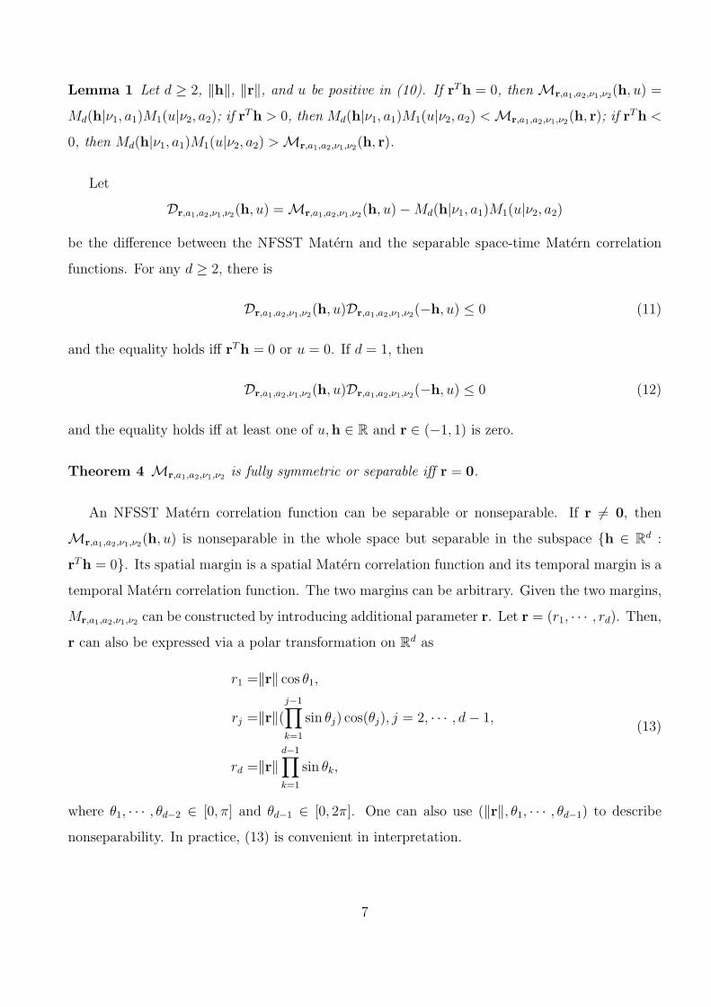
Lemma 1 Let d ≥ 2, ∥h∥, ∥r∥, and u be positive in (10). If rTh = 0, then Mr,a1,a2,ν1,ν2(h, u) =

Md(h|ν1, a1)M1(u|ν2, a2); if rTh > 0, then Md(h|ν1, a1)M1(u|ν2, a2) < Mr,a1,a2,ν1,ν2(h, r); if rTh <

0, then Md(h|ν1, a1)M1(u|ν2, a2) > Mr,a1,a2,ν1,ν2(h, r).

Let

Dr,a1,a2,ν1,ν2(h, u) = Mr,a1,a2,ν1,ν2(h, u)−Md(h|ν1, a1)M1(u|ν2, a2)

be the difference between the NFSST Matern and the separable space-time Matern correlation

functions. For any d ≥ 2, there is

Dr,a1,a2,ν1,ν2(h, u)Dr,a1,a2,ν1,ν2(−h, u) ≤ 0 (11)

and the equality holds iff rTh = 0 or u = 0. If d = 1, then

Dr,a1,a2,ν1,ν2(h, u)Dr,a1,a2,ν1,ν2(−h, u) ≤ 0 (12)

and the equality holds iff at least one of u,h ∈ R and r ∈ (−1, 1) is zero.

Theorem 4 Mr,a1,a2,ν1,ν2 is fully symmetric or separable iff r = 0.

An NFSST Matern correlation function can be separable or nonseparable. If r = 0, then

Mr,a1,a2,ν1,ν2(h, u) is nonseparable in the whole space but separable in the subspace {h ∈ Rd :

rTh = 0}. Its spatial margin is a spatial Matern correlation function and its temporal margin is a

temporal Matern correlation function. The two margins can be arbitrary. Given the two margins,

Mr,a1,a2,ν1,ν2 can be constructed by introducing additional parameter r. Let r = (r1, · · · , rd). Then,

r can also be expressed via a polar transformation on Rd as

r1 =∥r∥ cos θ1,

rj =∥r∥(j−1∏k=1

sin θj) cos(θj), j = 2, · · · , d− 1,

rd =∥r∥d−1∏k=1

sin θk,

(13)

where θ1, · · · , θd−2 ∈ [0, π] and θd−1 ∈ [0, 2π]. One can also use (∥r∥, θ1, · · · , θd−1) to describe

nonseparability. In practice, (13) is convenient in interpretation.

7

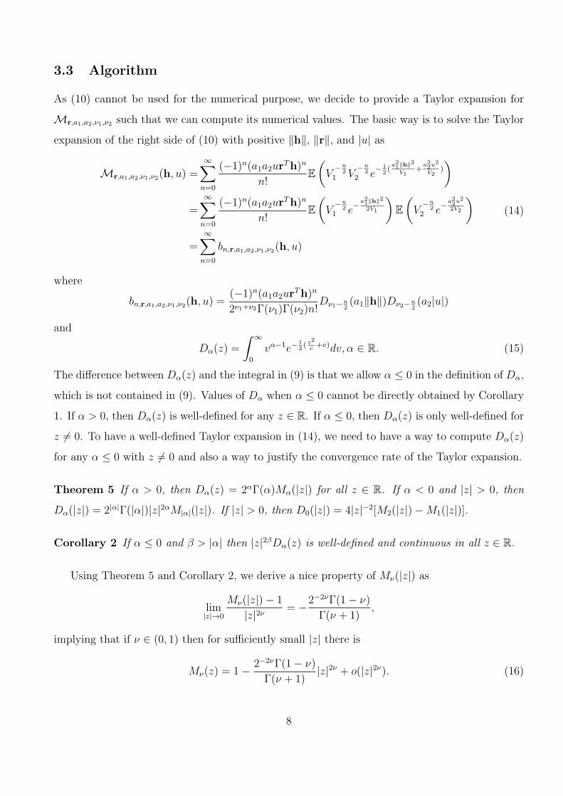
3.3 Algorithm

As (10) cannot be used for the numerical purpose, we decide to provide a Taylor expansion for

Mr,a1,a2,ν1,ν2 such that we can compute its numerical values. The basic way is to solve the Taylor

expansion of the right side of (10) with positive ∥h∥, ∥r∥, and |u| as

Mr,a1,a2,ν1,ν2(h, u) =∞∑n=0

(−1)n(a1a2urTh)n

n!E(V

−n2

1 V−n

22 e

− 12(a21∥h∥2

V1+

a22u2

V2)

)=

∞∑n=0

(−1)n(a1a2urTh)n

n!E(V

−n2

1 e−a21∥h∥2

2V1

)E(V

−n2

2 e−a22u

2

2V2

)=

∞∑n=0

bn,r,a1,a2,ν1,ν2(h, u)

(14)

where

bn,r,a1,a2,ν1,ν2(h, u) =(−1)n(a1a2ur

Th)n

2ν1+ν2Γ(ν1)Γ(ν2)n!Dν1−n

2(a1∥h∥)Dν2−n

2(a2|u|)

and

Dα(z) =

∫ ∞

0

vα−1e−12( z

2

v+v)dv, α ∈ R. (15)

The difference between Dα(z) and the integral in (9) is that we allow α ≤ 0 in the definition of Dα,

which is not contained in (9). Values of Dα when α ≤ 0 cannot be directly obtained by Corollary

1. If α > 0, then Dα(z) is well-defined for any z ∈ R. If α ≤ 0, then Dα(z) is only well-defined for

z = 0. To have a well-defined Taylor expansion in (14), we need to have a way to compute Dα(z)

for any α ≤ 0 with z = 0 and also a way to justify the convergence rate of the Taylor expansion.

Theorem 5 If α > 0, then Dα(z) = 2αΓ(α)Mα(|z|) for all z ∈ R. If α < 0 and |z| > 0, then

Dα(|z|) = 2|α|Γ(|α|)|z|2αM|α|(|z|). If |z| > 0, then D0(|z|) = 4|z|−2[M2(|z|)−M1(|z|)].

Corollary 2 If α ≤ 0 and β > |α| then |z|2βDα(z) is well-defined and continuous in all z ∈ R.

Using Theorem 5 and Corollary 2, we derive a nice property of Mν(|z|) as

lim|z|→0

Mν(|z|)− 1

|z|2ν= −2−2νΓ(1− ν)

Γ(ν + 1),

implying that if ν ∈ (0, 1) then for sufficiently small |z| there is

Mν(z) = 1− 2−2νΓ(1− ν)

Γ(ν + 1)|z|2ν + o(|z|2ν). (16)

8

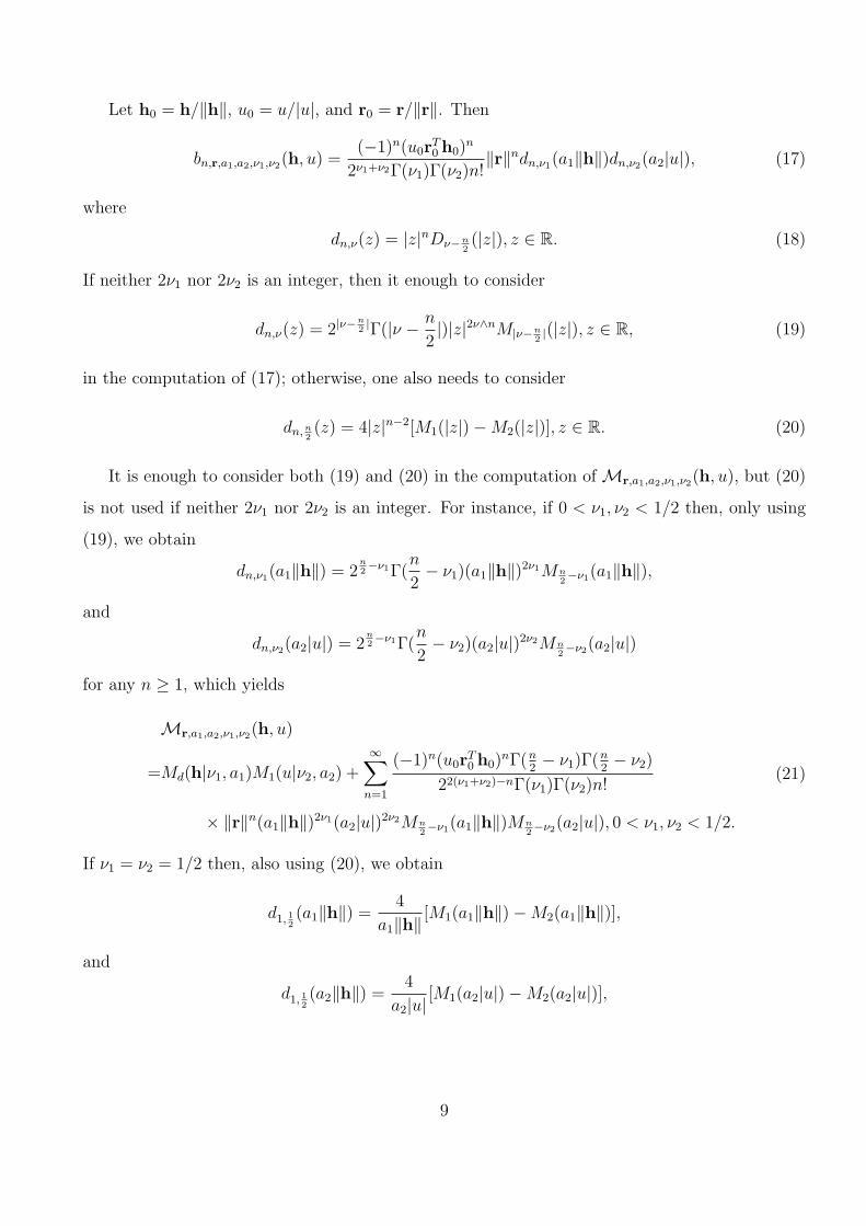
Let h0 = h/∥h∥, u0 = u/|u|, and r0 = r/∥r∥. Then

bn,r,a1,a2,ν1,ν2(h, u) =(−1)n(u0r

T0 h0)

n

2ν1+ν2Γ(ν1)Γ(ν2)n!∥r∥ndn,ν1(a1∥h∥)dn,ν2(a2|u|), (17)

where

dn,ν(z) = |z|nDν−n2(|z|), z ∈ R. (18)

If neither 2ν1 nor 2ν2 is an integer, then it enough to consider

dn,ν(z) = 2|ν−n2|Γ(|ν − n

2|)|z|2ν∧nM|ν−n

2|(|z|), z ∈ R, (19)

in the computation of (17); otherwise, one also needs to consider

dn,n2(z) = 4|z|n−2[M1(|z|)−M2(|z|)], z ∈ R. (20)

It is enough to consider both (19) and (20) in the computation of Mr,a1,a2,ν1,ν2(h, u), but (20)

is not used if neither 2ν1 nor 2ν2 is an integer. For instance, if 0 < ν1, ν2 < 1/2 then, only using

(19), we obtain

dn,ν1(a1∥h∥) = 2n2−ν1Γ(

n

2− ν1)(a1∥h∥)2ν1Mn

2−ν1(a1∥h∥),

and

dn,ν2(a2|u|) = 2n2−ν1Γ(

n

2− ν2)(a2|u|)2ν2Mn

2−ν2(a2|u|)

for any n ≥ 1, which yields

Mr,a1,a2,ν1,ν2(h, u)

=Md(h|ν1, a1)M1(u|ν2, a2) +∞∑n=1

(−1)n(u0rT0 h0)

nΓ(n2− ν1)Γ(

n2− ν2)

22(ν1+ν2)−nΓ(ν1)Γ(ν2)n!

× ∥r∥n(a1∥h∥)2ν1(a2|u|)2ν2Mn2−ν1(a1∥h∥)Mn

2−ν2(a2|u|), 0 < ν1, ν2 < 1/2.

(21)

If ν1 = ν2 = 1/2 then, also using (20), we obtain

d1, 12(a1∥h∥) =

4

a1∥h∥[M1(a1∥h∥)−M2(a1∥h∥)],

and

d1, 12(a2∥h∥) =

4

a2|u|[M1(a2|u|)−M2(a2|u|)],

9

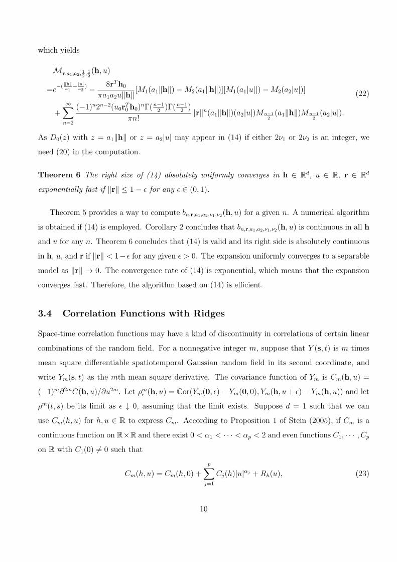
which yields

Mr,a1,a2,12, 12(h, u)

=e−(

∥h∥a1

+|u|a2

) − 8rTh0

πa1a2u∥h∥[M1(a1∥h∥)−M2(a1∥h∥)][M1(a1|u||)−M2(a2|u|)]

+∞∑n=2

(−1)n2n−2(u0rT0 h0)

nΓ(n−12)Γ(n−1

2)

πn!∥r∥n(a1∥h∥)(a2|u|)Mn−1

2(a1∥h∥)Mn−1

2(a2|u|).

(22)

As D0(z) with z = a1∥h∥ or z = a2|u| may appear in (14) if either 2ν1 or 2ν2 is an integer, we

need (20) in the computation.

Theorem 6 The right size of (14) absolutely uniformly converges in h ∈ Rd, u ∈ R, r ∈ Rd

exponentially fast if ∥r∥ ≤ 1− ϵ for any ϵ ∈ (0, 1).

Theorem 5 provides a way to compute bn,r,a1,a2,ν1,ν2(h, u) for a given n. A numerical algorithm

is obtained if (14) is employed. Corollary 2 concludes that bn,r,a1,a2,ν1,ν2(h, u) is continuous in all h

and u for any n. Theorem 6 concludes that (14) is valid and its right side is absolutely continuous

in h, u, and r if ∥r∥ < 1− ϵ for any given ϵ > 0. The expansion uniformly converges to a separable

model as ∥r∥ → 0. The convergence rate of (14) is exponential, which means that the expansion

converges fast. Therefore, the algorithm based on (14) is efficient.

3.4 Correlation Functions with Ridges

Space-time correlation functions may have a kind of discontinuity in correlations of certain linear

combinations of the random field. For a nonnegative integer m, suppose that Y (s, t) is m times

mean square differentiable spatiotemporal Gaussian random field in its second coordinate, and

write Ym(s, t) as the mth mean square derivative. The covariance function of Ym is Cm(h, u) =

(−1)m∂2mC(h, u)/∂u2m. Let ρmϵ (h, u) = Cor(Ym(0, ϵ)− Ym(0, 0), Ym(h, u+ ϵ)− Ym(h, u)) and let

ρm(t, s) be its limit as ϵ ↓ 0, assuming that the limit exists. Suppose d = 1 such that we can

use Cm(h, u) for h, u ∈ R to express Cm. According to Proposition 1 of Stein (2005), if Cm is a

continuous function on R×R and there exist 0 < α1 < · · · < αp < 2 and even functions C1, · · · , Cp

on R with C1(0) = 0 such that

Cm(h, u) = Cm(h, 0) +

p∑j=1

Cj(h)|u|αj +Rh(u), (23)

10

where Rh(u) = O(u2) as u → 0 for any given h and Rh(·) has a bounded second derivative, then

supu∈R

limϵ↓0

∣∣∣∣C1(h){|u+ ϵ|α1 − 2|u|α1 + |u− ϵ|α1

2C1(0)ϵα1− ρmϵ (h, u)

∣∣∣∣ = 0, (24)

where

ρm(h, u) =

C1(h)/C1(0), u = 0,

0, u = 0.

Assume (23) holds for m = 0. Using (24) with m = 0 for ρ0(h, u), one can consider the mean

squared error (MSE) of the ordinary kriging predictor of Y (0, ϵ) based on Y (0, 0), Y (h, 0), and

Y (h, ϵ), which is 2{C0(0)−C21(h)/C1(0)}ϵα1+o(ϵα1). As the MSE of the ordinary kriging predictor

of Y (0, ϵ) based on Y (0, 0) is 2C1(0)ϵα1 + o(ϵα1), the lack of continuity of ρ0(h, u) along the h

axis leads to best linear unbiased predictors that depend on observations whose correlations are

bounded away from 1 as ϵ ↓ 0, implying that correlation functions satisfying (23) have ridges

along their axes. Stein (2005) points out that many separable correlation functions satisfy (23).

All examples of Cressie and Huang (1999) satisfy (23). The sum of product form models with

functions of just space and just time (De Iaco, Myers, and Posa, 2001) may share ridges along

their axes. It would appear that nonseparable covariance functions proposed by Gneiting (2002)

may not be smoother along their axes than at the origin.

For a fully symmetric space-time correlation function C(h, u) on R×R. If there is an 0 < α1 < 2

such that 0 = C1(h) = limu↓0 u−α1 [C(h, u) − C(h, 0)] exists, then for sufficiently small u there is

C(−h, |u|) = C(h, |u|) = C(h, 0)+C1(h)|u|α1 +O(|u|α1), implying that C1(h) is an even function.

Therefore, a fully symmetric space-time correlation probably satisfies (23).

As our family is not fully symmetric, we consider a possible expansion related to (23). It is

obtained if (16), (17), and (19) are combined. In particular, we consider the Taylor expansion for

given h and r satisfying rTh = 0. We conclude that for sufficiently small u with ν2 ∈ (0, 1/2)

there is

Mr,1,1,ν1,ν2(h, u) =Mν1(∥h∥)− sign(urTh)C1(∥h∥)|u|2ν2 + C2(∥h∥)|u|2ν2 + o(|u|2ν2),

where C1(∥h∥) > 0. Therefore, our model does not satisfy (23), implying that Mr,a1,a2,ν1,ν2 does

not belong to the covariance family with a covariance ridge problem considered by Proposition 1

of Stein (2005).

11

(a): u=0

h1

h 2

0.78

0.78

0.78

0.78

0.8

0.8

0.8

0.8 0.82

0.84

0.86

0.88

0.9

0.92

0.94

0.96

−0.10 −0.05 0.00 0.05 0.10

−0.

10−

0.05

0.00

0.05

0.10

(b): u=0.1

h1

h 2

0.62

0.62

0.64 0.66

0.66

0.66

0.68

0.7

0.72

0.74

0.76

0.78

−0.10 −0.05 0.00 0.05 0.10

−0.

10−

0.05

0.00

0.05

0.10

(c): u=0.2

h1

h 2

0.54

0.54

0.56

0.58

0.6

0.62

0.64

0.66

0.68

−0.10 −0.05 0.00 0.05 0.10

−0.

10−

0.05

0.00

0.05

0.10

(d): u=0.5

h1

h 2

0.3

5

0.35

0.36

0.36

0.37

0.38 0.39

0.4

0.41

0.42

0.43

0.44

0.45

0.46

0.47

−0.10 −0.05 0.00 0.05 0.10

−0.

10−

0.05

0.00

0.05

0.10

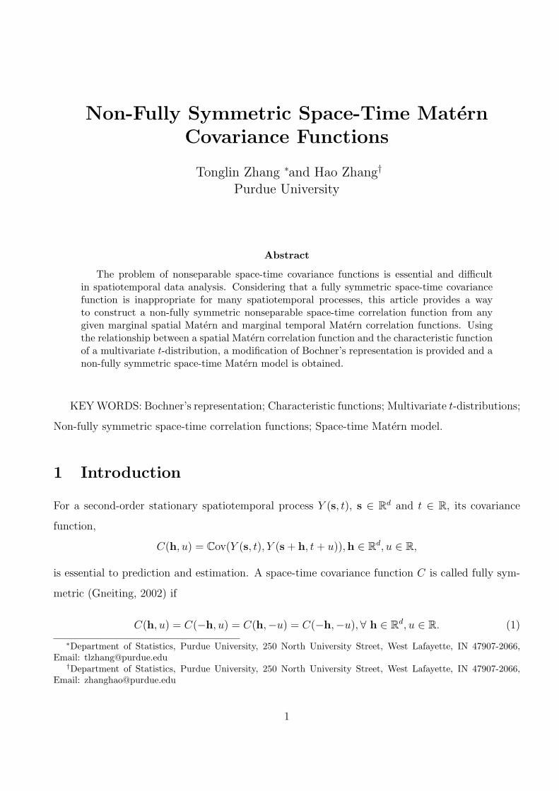
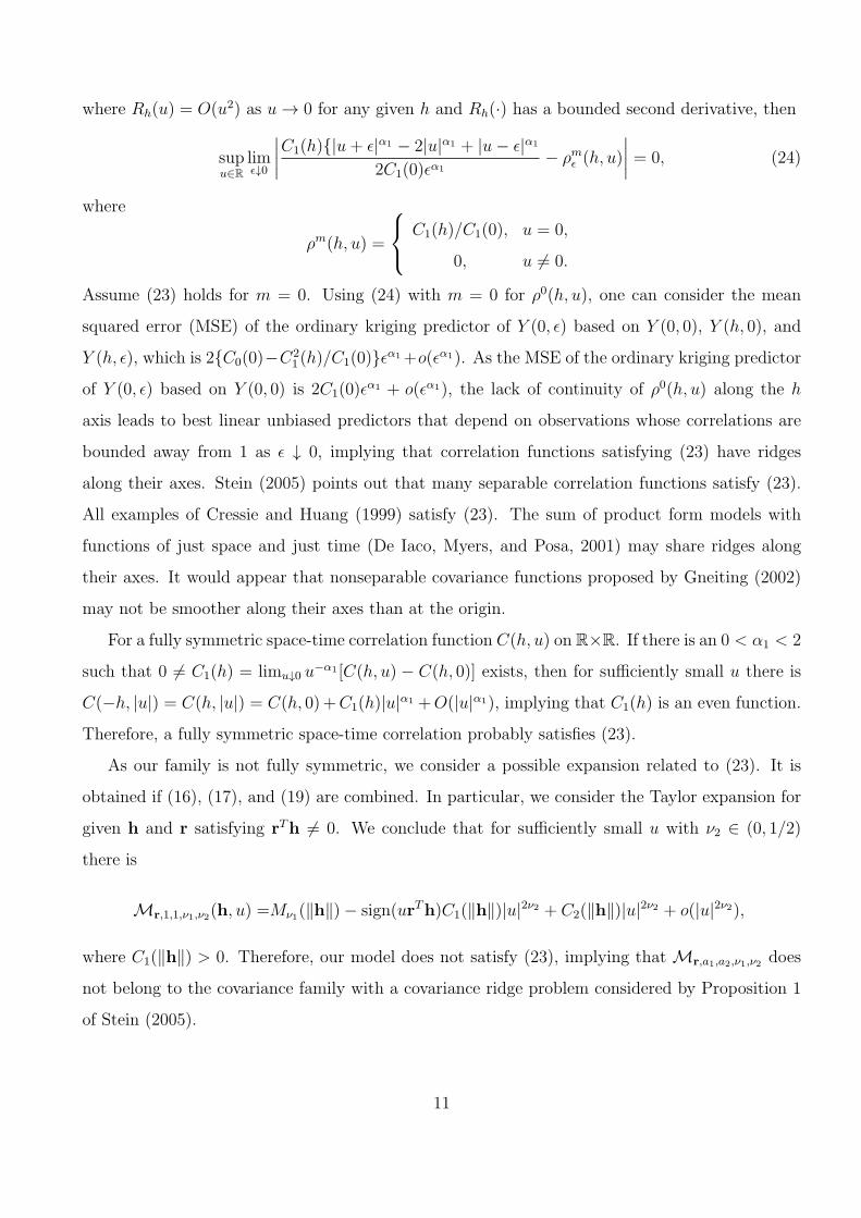
Figure 1: Contour plots for Mr,a1,a2,ν1,ν2(h, u) as functions of h = (h1, h2) for selected u when

r = (0.5, 0), a1 = a2 = 1, and ν1 = ν2 = 0.35.

3.5 The Case When d = 2

We specify Mr,a1,a2,ν1,ν2(h, u) in the case when d = 2 since it is important in practice. Let

r = (r1, r2) and h = (h1, h2) when d = 2. If ∥r∥ and ∥h∥ are positive, then h0 = (h01, h02) =

(h1/∥h∥, h2/∥h∥) and r0 = (r01, r02) = (r1/∥r∥, r2/∥r∥) are well defined. Equation (10) becomes

Mr,a1,a2,ν1,ν2(h, u) = E[(

e−a1a2u0|u||∥r∥∥h∥(r01h01+r02h02)√

V1V2

)(e− 1

2(a21∥h∥2

V1+

a22u2

V2)

)]. (25)

If u0 > 0 then, given |u| and ∥h∥, Mr,a1,a2,ν1,ν2(h, u) is minimized at h0 = r0 and maximized at

h0 = −r0; otherwise, Mr,a1,a2,ν1,ν2(h, u) is maximized at h0 = r0 and minimized at h0 = −r0.

If h0 and u0 are vertical, then Mr,a1,a2,ν1,ν2(h, u) = M2(h|ν1, a1)M1(u|ν2, a2). This is satisfied if

r01h01 + r02h02 = 0.

To study the performance of M in the spatial domain, we use (17) to numerically compute

the values of the correlation function on the left side of (25) for selected u when r = (0.5, 0),

a1 = a2 = 1, and ν1 = ν2 = 0.35 (Figure 1). It shows that the right side of (25) reduces to

M2(h|ν1, a1) if u = 0 (Figure 1(a)). The contour plots are more symmetric for small positive

u values than those for large positive u values. The values of the correlation function strictly

decreases in |u| or ∥h∥ increases along a certain direction. The speed of the decrease depends

12

(a): r=(0,0)

h1

h 2

0.38

0.38

0.38

0.38

0.39

0.39

0.39

0.39 0.4

0.41

0.42

0.43

0.44

0.45

0.46

−0.10 −0.05 0.00 0.05 0.10

−0.

10−

0.05

0.00

0.05

0.10

(b): r=(0.1,0)

h1

h 2

0.37

0.37

0.38

0.38

0.38

0.38

0.39

0.39

0.39 0.4

0.41

0.42

0.43

0.44

0.45

0.46

−0.10 −0.05 0.00 0.05 0.10

−0.

10−

0.05

0.00

0.05

0.10

(c): r=(0.2,0)

h1

h 2

0.37

0.37

0.38 0.39

0.39

0.39

0.4

0.41

0.42

0.43

0.44

0.45

0.46

−0.10 −0.05 0.00 0.05 0.10

−0.

10−

0.05

0.00

0.05

0.10

(d): r=(0.5,0)

h1

h 2

0.3

5

0.35

0.36

0.36

0.37

0.38 0.39

0.4

0.41

0.42

0.43

0.44

0.45

0.46

0.47

−0.10 −0.05 0.00 0.05 0.10

−0.

10−

0.05

0.00

0.05

0.10

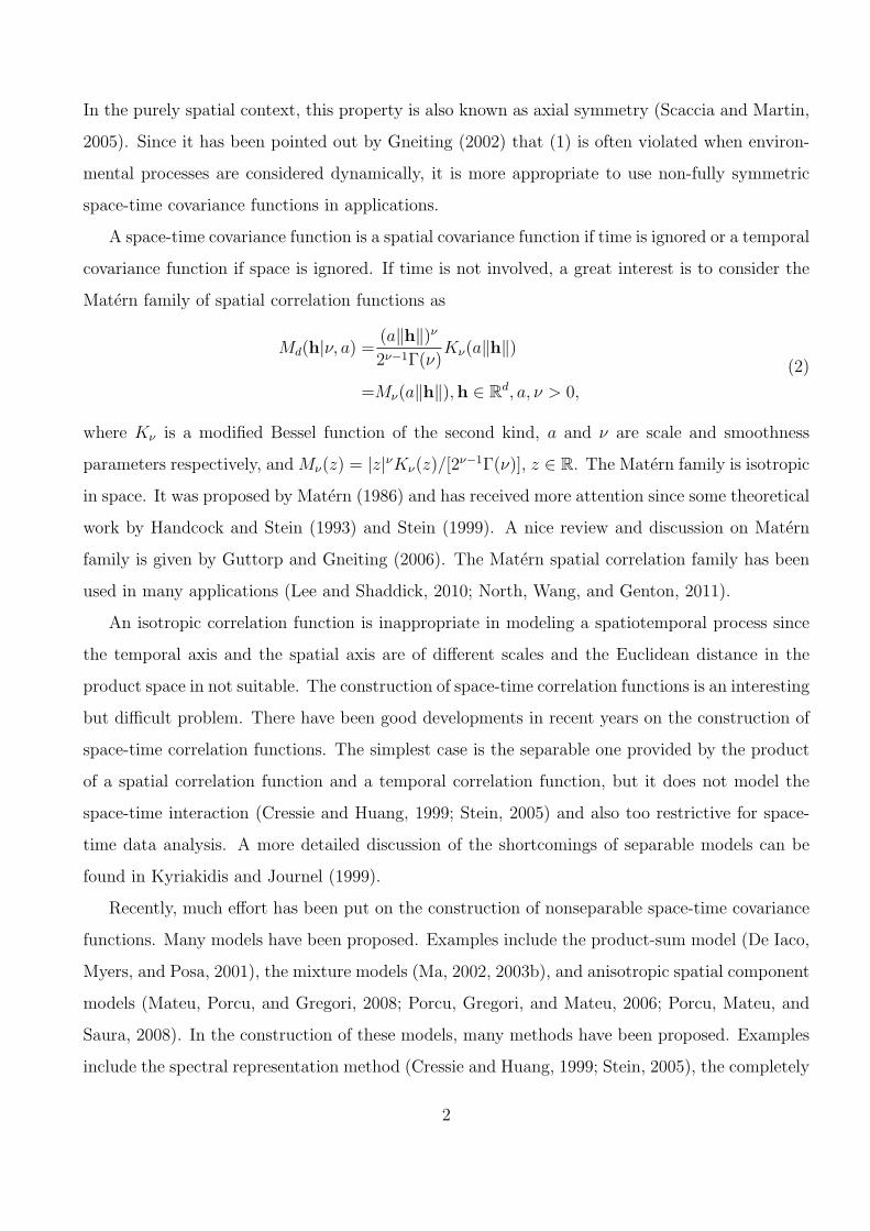
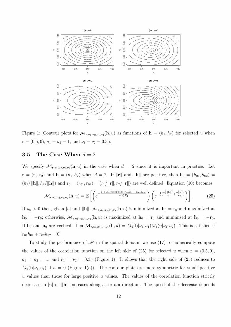
Figure 2: Contour plots for Mr,a1,a2,ν1,ν2(h, u) as functions of h = (h1, h2) for selected r when

u = 0.5, a1 = a2 = 1, and ν1 = ν2 = 0.35.

on the direction of r, which is maximized at the positive direction but minimized at the negative

direction of r.

To compare, we also use (17) to study the performance of M in the spatial domain when r

varies. We numerically compute the values of the correlation function on the left side of (25) for

selected r when u = 0.5, a1 = a2 = 1, and ν1 = ν2 = 0.35 (Figure 2). It shows that curves in

Figure 1(a) and Figure 2(a) are parallel. Both of them are isotropic. Values of curves in Figure

2(a) equals values of curves in Figure 1(a) multiplied by M0.35(0.5) = 0.4815. Curves in the rest

plots of Figure 2 are not isotropic. The magnitude of anisotropy increases as ∥r∥ increases. Curves

in Figure 1(d) and Figure 2(d) are identical. They provide the extremely anisotropic case in those

displayed in Figure 2.

Note that both r and h can be expressed by their norms and their angles. We also use the

polar coordinates to express the Taylor expansion of Mr,a1,a2,ν1,ν2(h, u). The result based on

the polar transformation is easy to interpret. Let the angle of r be ω and the angle of h be η,

ω, η ∈ (−π, π]. Then, r = (r1, r2) = (∥r∥ cosω, ∥r∥ sinω), h = (h1, h2) = (∥h∥ cos η, ∥h∥ sin η),

and rTh = r1h1 + r2h2 = ∥r∥∥h∥ cos(ω − η), which yields cos(ω − η) = (r1h1 + r2h2)/(∥r∥∥h∥) =

13

(a): η=0

u

||h||

0.2

0.3

0.4

0.4

0.5 0.6

0.7 0.8 0

.9

−0.4 −0.2 0.0 0.2 0.4

0.0

0.1

0.2

0.3

0.4

0.5

(b): η=π 8

u

||h||

0.3

0.3

0.4

0.4

0.5 0.6

0.7 0.8 0

.9

−0.4 −0.2 0.0 0.2 0.4

0.0

0.1

0.2

0.3

0.4

0.5

(c): η=π 4

u

||h||

0.3

0.3

0.4

0.4

0.5 0.6

0.7 0.8

0.9

−0.4 −0.2 0.0 0.2 0.4

0.0

0.1

0.2

0.3

0.4

0.5

(d): η=π 2

u

||h||

0.3

0.3

0.4 0.4

0.5 0.6

0.7 0.8

0.9

−0.4 −0.2 0.0 0.2 0.4

0.0

0.1

0.2

0.3

0.4

0.5

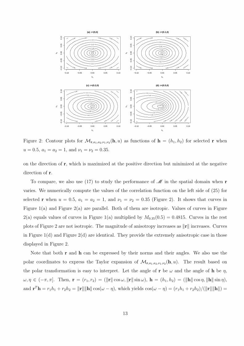
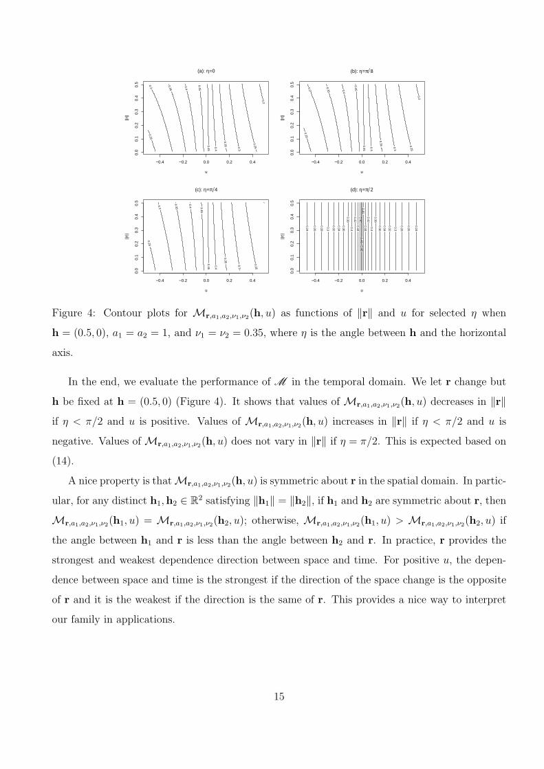
Figure 3: Contour plots for Mr,a1,a2,ν1,ν2(h, u) as functions of ∥h∥ and u for selected η when

r = (0.5, 0), a1 = a2 = 1, and ν1 = ν2 = 0.35, where η is the angle between h and the horizontal

axis.

r01h01 + r02h02 and

bn,r,a1,a2,ν1,ν2(h, u) =[−sign(u) cos(ω − η)]n

2ν1+ν2Γ(ν1)Γ(ν2)n!∥r∥ndn,ν1(a1∥h∥)dn,ν2(a2|u|). (26)

If u and ∥h∥ are positive, then Mr,a1,a2,ν1,ν2(h, u) < M2(h|ν1, a1)M1(u|ν2, a2) if |ω − η| < π/2

and Mr,a1,a2,ν1,ν2(h, u) > M2(h|ν1, a1)M1(u|ν2, a2) if |ω − η| > π/2. Using the polar expression of

bn,r,a1,a2,ν1,ν2(h, u) in (26), we can also interpret Figure 1 according to a rotation of r: if r is rotated

by an orthogonal transformation then the corresponding contour plot of Mr,a1,a2,ν1,ν2(h, u) is also

rotated with the same angle of the transformation.

To study the performance of M in the spatiotemporal domain, we use (26) to numerically

compute the values of Mr,a1,a2,ν1,ν2(h, u) (Figure 3). We still use r = (0.5, 0), a1 = a2 = 1, and

ν1 = ν2 = 0.35 in the computation such that ω = 0 and cos(ω − η) = cos η in (26). It shows

that the value of the correlation function is not symmetric about zero in u when η = π/2. If

η = π/2, then cos(η) = 0, implying that Mr,a1,a2,ν1,ν2(h, u) is separable. If η ∈ (π/2, π], then

cos(η) = − cos(π−η), implying that corresponding plots for η ∈ [π/2, π] can be derived by simply

reflecting the plots for η ∈ [0, π/2]. Note that Mr,a1,a2,ν1,ν2(h, u) is only separable in the sub-space

{h ∈ R2 : η = π/2}. The lower-right panel in Figure 3 is just a special case of Lemma 1.

14

(a): η=0

u

||r||

0.2

0.25

0.25

0.3

0.3

0.35

0.35

0.4

0.4

0.45

0.45

−0.4 −0.2 0.0 0.2 0.4

0.0

0.1

0.2

0.3

0.4

0.5

(b): η=π 8

u

||r||

0.2

0.25

0.25

0.3

0.3

0.35

0.35

0.4

0.4

0.45

0.45

−0.4 −0.2 0.0 0.2 0.4

0.0

0.1

0.2

0.3

0.4

0.5

(c): η=π 4

u

||r||

0.25

0.25

0.3

0.3

0.35

0.35

0.4

0.4

0.45

0.45

−0.4 −0.2 0.0 0.2 0.4

0.0

0.1

0.2

0.3

0.4

0.5

(d): η=π 2

u

||r||

0.24

0.24

0.26

0.26

0.28

0.28

0.3

0.3

0.32

0.32

0.34

0.34

0.36

0.36

0.38

0.38

0.4

0.4

0.42

0.42

0.44

0.44

0.46 0.46

0.48 0.48

−0.4 −0.2 0.0 0.2 0.4

0.0

0.1

0.2

0.3

0.4

0.5

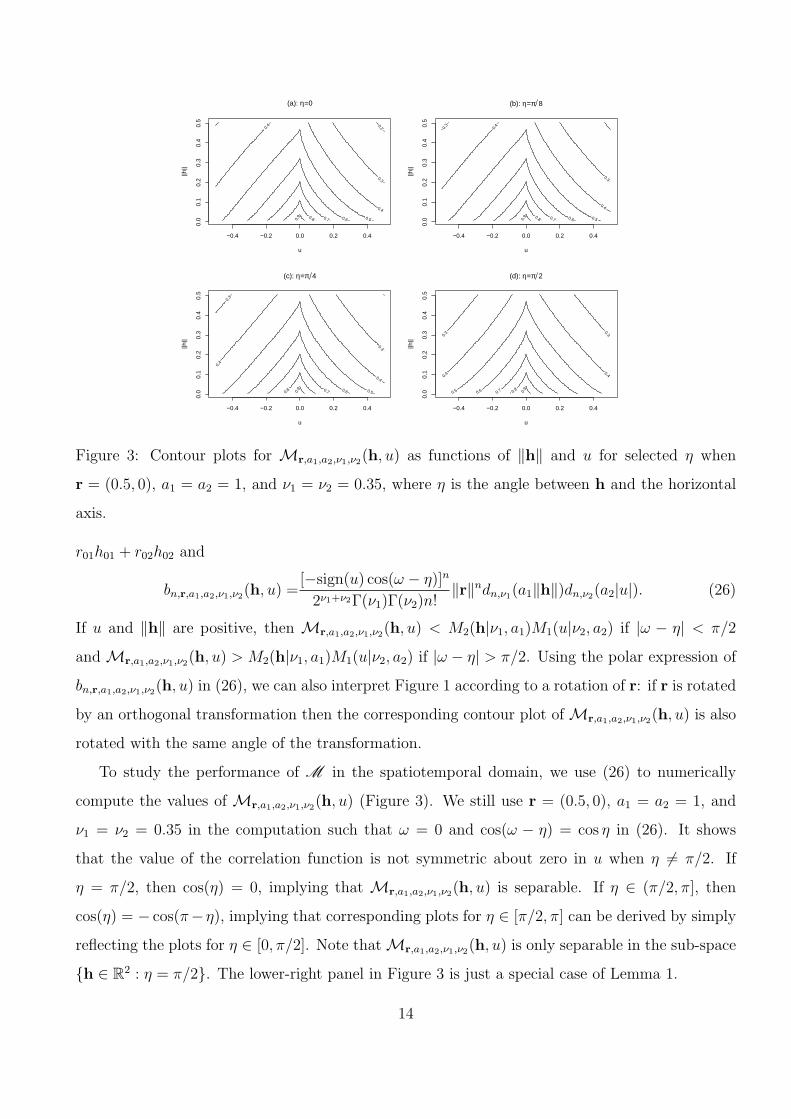
Figure 4: Contour plots for Mr,a1,a2,ν1,ν2(h, u) as functions of ∥r∥ and u for selected η when

h = (0.5, 0), a1 = a2 = 1, and ν1 = ν2 = 0.35, where η is the angle between h and the horizontal

axis.

In the end, we evaluate the performance of M in the temporal domain. We let r change but

h be fixed at h = (0.5, 0) (Figure 4). It shows that values of Mr,a1,a2,ν1,ν2(h, u) decreases in ∥r∥

if η < π/2 and u is positive. Values of Mr,a1,a2,ν1,ν2(h, u) increases in ∥r∥ if η < π/2 and u is

negative. Values of Mr,a1,a2,ν1,ν2(h, u) does not vary in ∥r∥ if η = π/2. This is expected based on

(14).

A nice property is thatMr,a1,a2,ν1,ν2(h, u) is symmetric about r in the spatial domain. In partic-

ular, for any distinct h1,h2 ∈ R2 satisfying ∥h1∥ = ∥h2∥, if h1 and h2 are symmetric about r, then

Mr,a1,a2,ν1,ν2(h1, u) = Mr,a1,a2,ν1,ν2(h2, u); otherwise, Mr,a1,a2,ν1,ν2(h1, u) > Mr,a1,a2,ν1,ν2(h2, u) if

the angle between h1 and r is less than the angle between h2 and r. In practice, r provides the

strongest and weakest dependence direction between space and time. For positive u, the depen-

dence between space and time is the strongest if the direction of the space change is the opposite

of r and it is the weakest if the direction is the same of r. This provides a nice way to interpret

our family in applications.

15

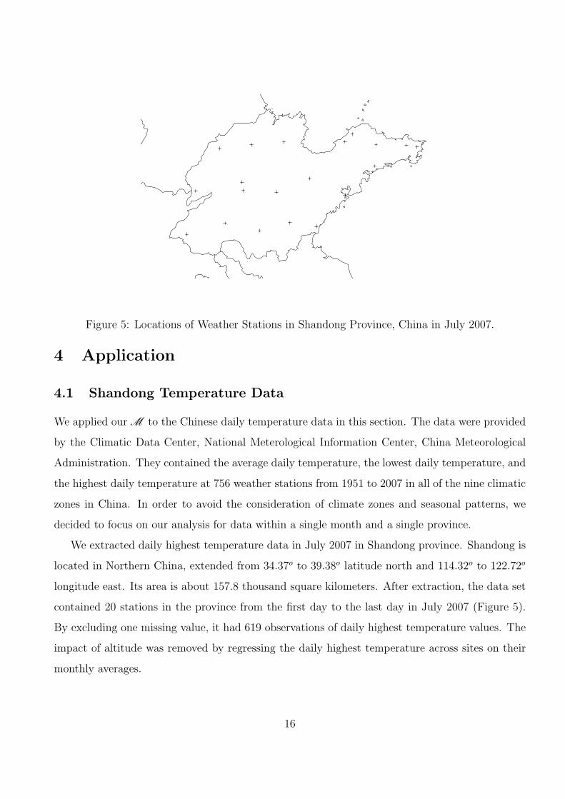
Figure 5: Locations of Weather Stations in Shandong Province, China in July 2007.

4 Application

4.1 Shandong Temperature Data

We applied our M to the Chinese daily temperature data in this section. The data were provided

by the Climatic Data Center, National Meterological Information Center, China Meteorological

Administration. They contained the average daily temperature, the lowest daily temperature, and

the highest daily temperature at 756 weather stations from 1951 to 2007 in all of the nine climatic

zones in China. In order to avoid the consideration of climate zones and seasonal patterns, we

decided to focus on our analysis for data within a single month and a single province.

We extracted daily highest temperature data in July 2007 in Shandong province. Shandong is

located in Northern China, extended from 34.37o to 39.38o latitude north and 114.32o to 122.72o

longitude east. Its area is about 157.8 thousand square kilometers. After extraction, the data set

contained 20 stations in the province from the first day to the last day in July 2007 (Figure 5).

By excluding one missing value, it had 619 observations of daily highest temperature values. The

impact of altitude was removed by regressing the daily highest temperature across sites on their

monthly averages.

16

Let Y (s, t) be the daily highest temperature relative to its site average. A geostatistical model

Y (s, t) = µ+ Z(s, t) + ϵ(s, t) (27)

was basically considered to analyze the spatiotemporal variations of Y (s, t), where ϵ(s, t) was a

white noise process and Z(s, t) was a mean zero stationary Gaussian process. The covariance

function of Z(s, t) was modeled by M as

E[Z(s, t)Z(s+ h, t+ u)] = τ 2Mr,a1,a2,ν1,ν2(h, u), (28)

where 1/a2 (given by km) and 1/a2 (given by day) were considered as two correlation lengths for

space and time, respectively. There were seven parameters on the right side of (28). Together the

variance parameter σ2 in the white noise process, our statistical model contained eight parameters

for the spatiotemporal variation of Y (s, t). We used η = σ2/(τ 2 + σ2) to represent the nugget

effect parameter and θ = (ν1, 1/a1, ν2, 1/a2, r1, r2) to represent the correlation parameters, where r1

represented the correlation between longitude and time and r2 represented the correlation between

latitude and time. The nugget effect disappeared if η = 0.

We attempted to estimate η and θ by the profile likelihood approach. In particular, let Y (si, ti),

i = 1, · · · , 619 be the ith observation in the data set. Then,

Cov[Y (si, ti), Y (sj, tj)] = (σ2 + τ 2)ρij = κ2ρij,

where

ρij = ρij(η, θ) = Corr[Y (si, ti), Y (sj, tj)] = (1− η)Mr,a1,a2,ν1,ν2(sj − si, tj − ti), i = j.

Let R = R(η, κ2) = (ρij)i,j=1,··· ,619 be the correlation matrix of the observations. The loglikelihood

function of the data was

ℓ(µ, κ2, η, θ) = −619

2log 2π − 1

2log κ2 − 1

2log | det(R)| − 1

2κ2(y − 1µ)′R−1(y − 1µ), (29)

where y = (Y (s1, t1), · · · , Y (s619, t619))′ and 1 is the vector with all of its elements equal to one.

Given η and θ, the conditional MLE of µ was

µ(η, θ) = (1′R−11)−11′R−1y (30)

and the conditional MLE of κ2 was

κ2(η, θ) =1

619[1′R−11− yR−11(1′R−11)−11′R−1y]. (31)

17

−250 −150 −50 0 50

0.40

0.45

0.50

0.55

0.60

(a): Parallel to r

Location Change

Sam

ple

Cor

rela

tions

−400 −200 0 200 400

0.40

0.45

0.50

0.55

0.60

(b): Vertical to r

Location ChangeS

ampl

e C

orre

latio

ns

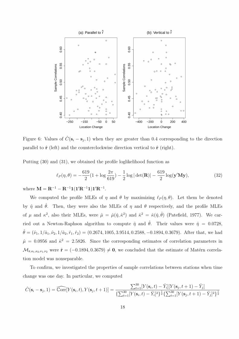
Figure 6: Values of C(si − sj, 1) when they are greater than 0.4 corresponding to the direction

parallel to r (left) and the counterclockwise direction vertical to r (right).

Putting (30) and (31), we obtained the profile loglikelihood function as

ℓP (η, θ) = −619

2(1 + log

2π

619)− 1

2log | det(R)| − 619

2log(y′My), (32)

where M = R−1 −R−11(1′R−11)1′R−1.

We computed the profile MLEs of η and θ by maximizing ℓP (η, θ). Let them be denoted

by η and θ. Then, they were also the MLEs of η and θ respectively, and the profile MLEs

of µ and κ2, also their MLEs, were µ = µ(η, κ2) and κ2 = κ(η, θ) (Patefield, 1977). We car-

ried out a Newton-Raphson algorithm to compute η and θ. Their values were η = 0.0728,

θ = (ν1, 1/a1, ν2, 1/a2, r1, r2) = (0.2674, 1005, 3.9514, 0.2588,−0.1894, 0.3679). After that, we had

µ = 0.0956 and κ2 = 2.5826. Since the corresponding estimates of correlation parameters in

Mr,a1,a2,ν1,ν2 were r = (−0.1894, 0.3679) = 0, we concluded that the estimate of Matern correla-

tion model was nonseparable.

To confirm, we investigated the properties of sample correlations between stations when time

change was one day. In particular, we computed

C(si − sj, 1) = Corr[Y (si, t), Y (sj, t+ 1)] =

∑30t=1[Y (si, t)− Yi][Y (sj, t+ 1)− Yj]

{∑30

t=1[Y (si, t)− Yi]2}12{∑30

t=1[Y (sj, t+ 1)− Yj]2}12

18

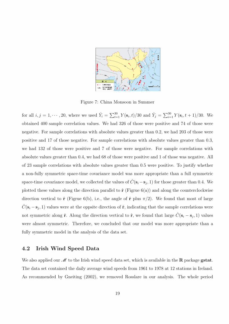
Figure 7: China Monsoon in Summer

for all i, j = 1, · · · , 20, where we used Yi =∑30

t=1 Y (si, t)/30 and Yj =∑30

i=1 Y (si, t + 1)/30. We

obtained 400 sample correlation values. We had 326 of those were positive and 74 of those were

negative. For sample correlations with absolute values greater than 0.2, we had 203 of those were

positive and 17 of those negative. For sample correlations with absolute values greater than 0.3,

we had 132 of those were positive and 7 of those were negative. For sample correlations with

absolute values greater than 0.4, we had 68 of those were positive and 1 of those was negative. All

of 23 sample correlations with absolute values greater than 0.5 were positive. To justify whether

a non-fully symmetric space-time covariance model was more appropriate than a full symmetric

space-time covariance model, we collected the values of C(si−sj, 1) for those greater than 0.4. We

plotted these values along the direction parallel to r (Figrue 6(a)) and along the counterclockwise

direction vertical to r (Figrue 6(b), i.e., the angle of r plus π/2). We found that most of large

C(si− sj, 1) values were at the oppsite direction of r, indicating that the sample correlations were

not symmetric along r. Along the direction vertical to r, we found that large C(si − sj, 1) values

were almost symmetric. Therefore, we concluded that our model was more appropriate than a

fully symmetric model in the analysis of the data set.

4.2 Irish Wind Speed Data

We also applied our M to the Irish wind speed data set, which is available in the R package gstat.

The data set contained the daily average wind speeds from 1961 to 1978 at 12 stations in Ireland.

As recommended by Gneiting (2002), we removed Rosslare in our analysis. The whole period

19

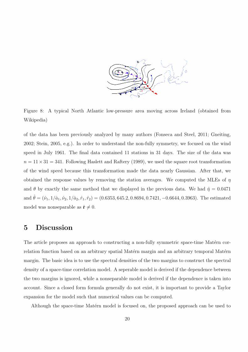
Figure 8: A typical North Atlantic low-pressure area moving across Ireland (obtained from

Wikipedia)

of the data has been previously analyzed by many authors (Fonseca and Steel, 2011; Gneiting,

2002; Stein, 2005, e.g.). In order to understand the non-fully symmetry, we focused on the wind

speed in July 1961. The final data contained 11 stations in 31 days. The size of the data was

n = 11× 31 = 341. Following Haslett and Raftery (1989), we used the square root transformation

of the wind speed because this transformation made the data nearly Gaussian. After that, we

obtained the response values by removing the station averages. We computed the MLEs of η

and θ by exactly the same method that we displayed in the previous data. We had η = 0.0471

and θ = (ν1, 1/a1, ν2, 1/a2, r1, r2) = (0.6353, 645.2, 0.8694, 0.7421,−0.6644, 0.3963). The estimated

model was nonseparable as r = 0.

5 Discussion

The article proposes an approach to constructing a non-fully symmetric space-time Matern cor-

relation function based on an arbitrary spatial Matern margin and an arbitrary temporal Matern

margin. The basic idea is to use the spectral densities of the two margins to construct the spectral

density of a space-time correlation model. A seperable model is derived if the dependence between

the two margins is ignored, while a nonseparable model is derived if the dependence is taken into

account. Since a closed form formula generally do not exist, it is important to provide a Taylor

expansion for the model such that numerical values can be computed.

Although the space-time Matern model is focused on, the proposed approach can be used to

20

construct other models. Theoretically, for any given A(h, u) in Theorem 1, infinite families of Z1

and Z2 can be selected. Therefore, the proposed approach can be used to construct infinite many

space-time correlation models, where one of those is the space-time Matern model that has been

discussed in the article. The nonseparable space-time Matern model contains two smoothness

parameters, two scale parameters, and a vector correlation parameter. The vector correlation

parameter provides the direction for dependence between space and time. The space-time de-

pendence is symmetric if the change of spatial locations belongs to the orthogonal space of the

correlation parameter; otherwise, non-full symmetry appears.

The significant difference between our proposed model and many previous models is the non-

full symmetry. The proposed approach directly provides a non-fully symmetric spectral density

in the space-time domain. One does not need to consider a way to make a space-time correlation

function non-fully symmetric via a certain transformation. As our model contains the separable

Matern correlation model as a special case, the justification of separability of spatiotemporal data

in geostatistics can be possibly defined as a hypothesis testing problem, and this is an interesting

and important research topic in the future.

A Proofs

Proof of Theorem 1: Let F be the spectral distribution of A(h, u). Without the loss of generality,

assume F is a probability measure, which is generated by a random vector x1 ∈ Rd and X2 ∈ R.

If (x1, X2) is independent of (Z1, Z2), then

A(hZ1, uZ2) = E(ei(Z1hTx1+Z2uX2)|Z1, Z2

)and

C(h, u) =

∫ ∞

0

∫ ∞

0

E[ei(z1h

Tx1+z2uX2)]G(dz1, dz2)

=E[E(ei(h

Tx1Z1+uX2Z2))|Z1, Z2

]=E

(ei(h

Tx1Z1+uX2Z2)).

Therefore, C(h, u) is a characteristic function of x1Z1 and X2Z2, implying that C(h, u) is a valid

space-time correlation function. If F is not a probability measure, then C(h, u) is a covariance

function but not a correlation function. ♢

21

Proof of Theorem 2: The sufficiency is directly implied by the expression of C(h, u). For the

necessity, if C(h, u) is separable then, using the uniqueness of the inverse Fourier transformation,

we conclude that Z1x1 and Z2X2 are independent. Since (x1, X2), Z1, and Z2 are independent,

(Z1x1, Z1) is independent of Z2 and (Z2x2, Z2) is independent of Z1. Let z1 and z2 be real values

such that P (Z1 ∈ dz1) and P (Z2 ∈ dz2) are positive if |dz1| and |dz2|, the Lebesgue measures of

dz1 and dz2 respectively, are positive. For any B1 ∈ B(Rd) and B2 ∈ B(R),

P (x1 ∈ B1, X2 ∈ B2)

= lim|dz1|→0,|dz2|→0

P (Z1x1 ∈ z1B1, Z2X2 ∈ z2B2|Z1 ∈ dz1, Z2 ∈ dz2)

= lim|dz1|→0,|dz2|→0

P (Z1x1 ∈ z1B1, Z2X2 ∈ z2B2, Z1 ∈ dz1, Z2 ∈ dz2)

P (Z1 ∈ dz1, Z2 ∈ dz2)

= lim|dz1|→0,|dz2|→0

P (Z1x1 ∈ z1B1, Z1 ∈ dz1)P (Z2X2 ∈ z2B2, Z2 ∈ dz2)

P (Z1 ∈ dz1)P (Z2 ∈ dz2)

= lim|dz1|→0,|dz2|→0

P (Z1x1 ∈ z1B1|Z1 ∈ dz1)P (Z2X2 ∈ z2B2|Z2 ∈ dz2)

=P (x1 ∈ B1)P (X2 ∈ B2).

Therefore, x1 and X2 are independent, implying that A(h, u) is separable. ♢

Proof of Theorem 3: The joint PDF of (u, V ) is

f1(u, v) =vν−1

2ν+d2π

d2Γ(ν)

e−12(∥u∥2+v).

The inverse transformation of (x, V ) = (au/√V , V ) is (u, v) = (

√V x/a, V ). The corresponding

Jacabian determinant is (V/a)d2 . The joint PDF of (x, V ) is

f2(x, v) =vν+

d2−1

2ν+d2a

d2π

d2Γ(ν)

e−12(1+

∥x∥2

a2)v.

Integrationg out v in f2(x, v), we obtain the marginal PDF of x, which is md(x|ν, a), implying

that the characteristic function of x is Md(h|ν, a). ♢

Proof of Corollary 1: Straightforwardly, there is

Md(h|ν, a) = E(eih

Tx)= E

[E(eih

T (au/√V )|V

)]= E

(e−

a2∥h∥22V

),

which yields (8). ♢

Proof of Lemma 1: The conclusion is implied by comparing

Mr,a1,a2,ν1,ν2(h, u) = E

(e−a1a2ur

T h√V1V2 e

− 12(a21∥h∥2

V1+

a22u2

V2)

)

22

with

Md(h|ν1, a1)M1(h|ν2, a2) = E(e− 1

2(a21∥h∥2

V1+

a22u2

V2)

),

since it is drawn by looking at the sign of rTh. ♢

Proof of Theorem 4: The necessary and sufficient conditions for Mr,a1,a2,ν1,ν2 to be separable

is implied by Theorem 2. The sufficiency of full symmetry is concluded using the definition of

Mr,a1,a2,ν1,ν2 . If d ≥ 2 then the necessity of full symmetry is implied by (11). If d = 1, then the

necessity of full symmetry is implied by (12). ♢

Proof of Theorem 5: The conclusion for α > 0 can be directly implied by (9). If α < 0 and

z = 0, using variable transformation w = z2/v in the integral expression of Dα(z) there is

Dα(z) = |z|2α∫ ∞

0

w−α−1e−12( z

2

w+w)dw = z2α

∫ ∞

0

w|α|−1e−12( z

2

w+w)dw = |z|2αD|α|(|z|),

implying the conclusion for α < 0. If α = 0, then

D0(z) =2

z2

∫ ∞

0

ve−v2 de−

z2

2v =2

z2

[∫ ∞

0

(v2− 1)e−

12( z

2

v+v)dv

]=

2

z2D2(z)−

1

z2D1(z),

implying the conclusion for α = 0. ♢

Proof of Corollary 2: If α < 0 then |z|2βDα(z) = 2|α|Γ(|α|)|z|2(β+α)M|α|(|z|) implying that it is

continuous in z ∈ R. Write

|z|2βD0(z) = |z|2β∫ 1

0

v−1e−12( z

2

v+v)dv + |z|2β

∫ ∞

1

v−1e−12( z

2

v+v)dv. (33)

The second term on the right side of (33) is continuous in z ∈ R. For any β > γ > 0, the first

term is dominated by

|z|2β∫ ∞

0

v−γ−1e−12( z

2

v+v)dz = |z|2βD−γ(z),

which is continuous in all z ∈ R. Letting γ → 0 and using the Dominated Convergence Theorem,

we conclude that the first term on the right side of (33) is also continuous in all z ∈ R. ♢

Proof of Theorem 6: If n > 2(ν1 ∨ n2), then

dn,ν1(a1∥h∥) = 2n2−ν1Γ(

n

2− ν1)(a1∥h∥)2ν1Mn

2−ν1(a1∥h∥)

and

dn,ν2(a2|u|) = 2n2−ν2Γ(

n

2− ν2)(a2|u|)2ν2Mn

2−ν2(a2|u|),

implying that

bn,r,a1,a2,ν1,ν2(h, u) =(−1)n(u0r

T0 h0)

n(a1∥h∥)2ν1(a2|u|)2ν222(ν1+ν2)Γ(ν1)Γ(ν2)

cn,ν1,ν2(a1∥h∥, a2|u|, ∥r∥),

23

where

cn,ν1,ν2(z1, z2, r) =2nrnΓ(n

2− ν1)Γ(

n2− ν2)

n!Mn

2−ν1(z1)Mn

2−ν2(z2), z1, z2, r > 0.

Note that

|bn,r,a1,a2,ν1,ν2(h, u)| ≤(a1∥h∥)2ν1(a2|u|)2ν222(ν1+ν2)Γ(ν1)Γ(ν2)

cn,ν1,ν2(a1∥h∥, a2|u|, ∥r∥)

and

cn,ν1,ν2(z1, z2, r) ≤ cn,ν1,ν2(r) =2nrnΓ(n

2− ν1)Γ(

n2− ν2)

n!, n > 2(ν1 ∨ ν2).

It is enough to show the uniform convergence of∑∞

n=[2(ν1∨n2)]+1] cn,ν1,ν2(r) in r ∈ [0, 1− ϵ] for any

0 < ϵ < 1. Using Stirling’s approximation that Γ(z) ≈√2πe−zzz−

12 (1 + o(1)) for sufficiently large

z, there is

limn→∞

cn+1,ν1,ν2(r)

cn,ν1,ν2(r)= lim

n→∞

2rΓ(n+12

− ν1)Γ(n+12

− ν2)

(n+ 1)Γ(n2− ν1)Γ(

n2− ν2)

= limn→∞

2r

n+ 1

(n+12

− ν1)n2−ν1(n+1

2− ν2)

n2−ν2e−(n+1−ν1−ν2)

(n2− ν1)

n−12

−ν1(n2− ν2)

n−12

−ν2e−(n−ν1−ν2)

= limn→∞

2r(n+12

− ν1)12 (n+1

2− ν2)

12

(n+ 1)e

(1 +

1

n− 2ν1

)n−12

−ν1 (1 +

1

n− 2ν2

)n−12

−ν2

=r.

Therefore,∑∞

n=[2(ν1∨ν2)]+1 dn,ν1,ν2(r) uniformly converges in r ≤ [0, 1 − ϵ] for any 0 < ϵ < 1,

implying that the right size of (14) absolutely uniformly converges in h ∈ Rd, u ∈ R, r ∈ Rd with

∥r∥ ≤ 1− ϵ for any 0 < ϵ < 1. ♢

References

Bochner, S. (1955). Harmonic Analysis and the Theory of Probability, Berkeley and Los Angeles:

University of California Press.

Brown, P., Karesen, K., Tonellato, G.O.R.S. (2000). Blur-generated nonseparable space-time mod-

els. Journal of Royal Statistical Society Series B, 62, 847-860.

Cressie, N. and Huang, H.C. (1999). Classes of nonseparable, spatio-temporal stationary covariance

functions. Journal of the American Statistical Association, 94, 1330–1340.

De Iaco, S., Myers, D., and Posa, D. (2001). Space-time analysis using a general product-sum

model. Statistics and Probability Letters, 52, 21-28.

24

De Iaco, S., Myers, D., and Posa, D. (2002). Nonseparable space-time covariance models: Some

parametric families. Mathematical Geology, 34, 23-41.

De Iaco, S., Posa, D., and Myers, D. (2013). Characteristics of some classes of Space-time covari-

ance functions. Journal of Statistical Planning and Inference, 143, 2002-2015.

De Iaco, S. and Posa, D. (2013). Positive and negative non-separability for space-time covariance

models. Journal of Statistical Planning and Inference, 143, 378-391.

Devroye, L. (1990). A note on Linnik distribution. Statistics and Probability Letters, 9, 305-306.

Fonseca, T.C.O. and Steel, M.F.J. (2011). A general class of nonseparable space-time correlation

functions. Environmentrics, 22, 224-242.

Fuentes, M. (2006). Testing for separability of spatial-temporal covariance functions. Journal of

Statistical Planning and Inference, 136, 447-466.

Gneiting, T. (2002). Nonseparable, stationary covariance functions for space-time data. Journal

of the American Statistical Association, 97, 590–600.

Gneiting, T., Genton, M.G., Guttorp, P. (2007). Geostatistical space-time models, stationarity,

separability, and full symmetry. In Statistical Methods for Spatiotemporal Systems, Finkenstadt,

B., Held, L., and Lsham, V. (eds). Chapman & Hall/CRC, 151-175.

Guttorp, P. and Gneiting, T. (2006). Studies in the history of probability and statistics XLIX: On

the Matern correlation family. Biometrika, 93, 989-995.

Handcock, M.S., and Stein, M.L. (1993). A Bayesian analysis of Kriging. Technometrics, 35,

403-410.

Haslett, J., and Raftery, A.E. (1989). Space-time modeling with long-memory dependence: assess-

ing Ireland’s wind power resources (with discussion). Applied Statistics, 38, 1-50.

Kolovos, A., Christakos, G., Hristopulos, D., and Serre, M. (2004). Methods for generating

non-separable spatiotemporal covariance models with potential environmental applications. Ad-

vances in Water Resources, 27, 815-830.

25

Kyriakidis, P.C. and Journel, A.G. (1999). Geostatistical space-time models: a review. Mathemat-

ical Geology, 31, 651-684.

Lee, D. and Shaddick, G. (2010). Spatial modeling of air pollution in studies of its short-term

health effects. Biometrics, 66, 1238-1246.

Li, B., Genton, M.G., Sherman, M. (2007). A nonparametric assessment of properties of space-time

covariance functions. Journal of the American Statistical Association, 102, 736-744.

Ma, C. (2002). Spatio-temporal covariance functions generated by mixtures.Mathematical Geology,

34, 965-975.

Ma, C. (2003). Families of spato-temporal stationary covariance models. Journal of Statistical

Planning and Inference, 116, 489-501.

Ma, C. (2003). Spatiotemporal stationary covariance models. Journal of Multivariate Analysis,

86, 97-107.

Ma, C. (2005). Linear combinations of space-time covariance functions and variograms. IEEE

Transactions on signal processing, 53, 857-864.

Mateu, J., Porcu, E., Gregori, P. (2008). Recent advances to model anisotropic space-time data.

Statistical Methods and Applications, 17, 209-223.

Matern, B. (1986). Spatial Variation (2nd ed.), Berlin: Springer-Verlag.

Mitchell M, Genton MG, Gumpertz M. (2005). Testing for separability of space-time covariances.

Environmetrics, 16, 819-831.

North, G., Wang, J. and Genton, M. (2011). Correlation models for temperature fields. Journal

of Climate, 24, 5850–5862.

Patefield, W.M. (1977). On the maximized likelihood function. Sankhya Series B, 39, 92-96.

Porcu, E., Gregori, P., Mateu, J. (2006). Nonseparable stationary anisotropic space-time covari-

ance functions. Stochastic Environmental Research and Risk Assessment, 21, 113-122.

26

Porcu, E., Mateu, J., and Saura, F. (2008). New classes of covariance and spectral density functions

for spatio-temporal modelling. Stochastic Environmental Research and Risk Assessment, 22, 65-

79.

Rodrigues, A. and Diggle, P. (2010). A class of convolution-based models for spatiotemporal

processes with non-separable covariance structure. Scandinavian Journal of Statistics, 37, 553-

567.

Scaccia, L. and Martin, R.J. (2005). Testing axial symmetry and separability of lattice processes.

Journal of Statistical Planning and Inference, 131, 19-39.

Shao, X. and Li, B., (2009). A tuning parameter free test for properties of spacetime covariance

functions. Journal of Statistical Planning and Inference, 139, 4031-4038.

Stein, M.L. (1999). Interpolation of Spatial Data. Some Theory for Kriging. New York: Springer-

Verlag.

Stein, M.L. (2005). Space-Time Covariance Functions. Journal of the American Statistical Asso-

ciation, 100, 310–321.

27