Non-hyperbolic common re ection surfacea - ahay.org · Non-hyperbolic common re ection surfacea aPublished in Geophysical Prospecting, 61, 21-27 (2013) Sergey Fomel and Roman Kazinniky

Non-hyperbolic common reflection surfacea

aPublished in Geophysical Prospecting, 61, 21-27 (2013)

Sergey Fomel∗ and Roman Kazinnik∗†

ABSTRACT

The method of common reflection surface (CRS) extend conventional stacking ofseismic traces over offset to multidimensional stacking over offset-midpoint sur-faces. We propose a new form of the stacking surface, derived from the analyticalsolution for reflection traveltime from a hyperbolic reflector. Both analyticalcomparisons and numerical tests show that the new approximation can be signif-icantly more accurate than the conventional CRS approximation at large offsetsor at large midpoint separations while using essentially the same parameters.

INTRODUCTION

Seismic data stacking is (together with deconvolution and migration) one of the fun-damental operations in seismic data analysis (Yilmaz, 2000). Conventional stackingoperates on common-midpoint (CMP) gathers and stacks traces after a hyperbolicmoveout. The method of multifocusing (MF), originally developed by Gelchinskyet al. (1999a,b) and modified to the common-reflection-surface (CRS) method byJager et al. (2001), stacks data from multiple CMP locations. As a result, the signal-to-noise ratio is improved considerably. Both MF and CRS require estimation ofmultiple parameters in addition to the conventional stacking velocity. These parame-ters correspond to the slope and curvature of seismic events in the midpoint directionand have physical interpretation in terms of wavefront slopes and curvatures. Manysuccessful applications of MF and CRS have been reported in the literature (Landaet al., 1999; Gurevich et al., 2002; Menyoli et al., 2004; Heilmann et al., 2006; Gierseet al., 2006; Hoecht et al., 2009).

The CRS method employs a multiparameter hyperbolic approximation of the re-flection traveltime surface (Tygel and Santos, 2007). The hyperbolic approximationcan be justified from a truncated Taylor series expansion of the squared traveltimearound a reference ray. As such, it is always accurate at small deviations from thecentral ray. However, it loses its accuracy at large offsets or large midpoint separa-tions.

In this paper, we propose a new nonhyperbolic approximation. The form of thisapproximation follows from an analytical equation for reflection traveltime from ahyperbolic reflector. The idea of approximation reflection traveltimes by approximat-ing reflector surfaces was first proposed by Moser and Landa (2009) and Landa et al.

Fomel & Kazinnik 2 Nonhyperbolic CRS

(2010). However, these publications did not provide a closed-form representation ofthe stacking surface. By analyzing the accuracy of the proposed nonhyperbolic ap-proximation on a number of examples, we show that the proposed approximation cansignificantly extend the accuracy range of CRS.

HYPERBOLIC AND NONHYPERBOLIC CRS

If P (t,m, h) represents the prestack seismic data as a function of time t, midpoint mand half-offset h, then conventional stacking can be described as

S(t0,m0) =

∫P (θ(h; t0),m0, h) dh , (1)

where S(t,m) is the stack section, and θ(h; t0) is the moveout approximation, whichmay take a form of a hyperbola

θ(h; t0) =

√t20 +

4h2

v2(2)

with v as an effective velocity parameter or, alternatively, a more complicated non-hyperbolic functional form, which involves other parameters (Fomel and Stovas, 2010).

The MF or CRS stacking takes a different form,

S(t0,m0) =

∫∫P(θ(m−m0, h; t0),m, h

)dmdh , (3)

where the integral over midpoint m is typically carried out only over a limited neigh-borhood of m0. The multifocusing approximation of Gelchinsky et al. (1999a) takesthe form

θMF (d, h; t0) = t0 + T(+)(d, h) + T(−)(d, h) , (4)

where, in the notation of Tygel et al. (1999),

T(±) =

√1 + 2K(±) (d± h) sin β +K2

(±) (d± h)2 − 1

V0K(±), (5)

K(±) =KN ± σKNIP

1± σ, (6)

and

σ(d, h) =h

d+KNIP sin β(d2 − h2). (7)

The four parameters {KN , KNIP , β, V0} have clear physical interpretations in termsof the wavefront and ray geometries (Gelchinsky et al., 1999a). V0 represents thevelocity at the surface and is typically assumed known and constant around thecentral ray. One important property of the MF approximation is that, in a constant


velocity medium with velocity V0, it can accurately describe both reflections from aplane dipping interfaces and diffractions from point diffractors.

The CRS approximation (Jager et al., 2001) is

θCRS(d, h; t0) =√F (d) + b2 h2 , (8)

where F (d) = (t0 + a1 d)2 + a2 d2, and the three parameters {a1, a2, b2} are related to

the multifocusing parameters as follows:

a1 =2 sin β

V0, (9)

a2 =2 cos2 β KN t0

V0, (10)

b2 =2 cos2 β KNIP t0

V0. (11)

Equation (8) is equivalent to a truncated Taylor expansion of the squared traveltimein equation (4) around d = 0 and h = 0. In comparison with MF, CRS possessesa fundamental simplicity, which makes it easy to extend the method to 3-D. How-ever, it looses the property of accurately describing diffractions in a constant-velocitymedium.

We propose the following modification of approximation (8):

θ(d, h; t0) =

√F (d) + c h2 +

√F (d− h)F (d+ h)

2, (12)

where c = 2 b2 + a21 − a2. Equation (12), which we call non-hyperbolic commonreflection surface, is derived in Appendix A. A truncated Taylor expansion of thesquared traveltime from equation (12) around d = 0 and h = 0 is equivalent toequation (8).

There are two important special cases:

1. If a2 = 0 or KN = 0, equation (12) becomes equivalent to equation (8), withF (d) = (t0 + a1 d)2. In a constant-velocity medium, this case corresponds toreflection from a planar reflector.

2. If a2 = b2 or KNIP = 0, equation (12) becomes equivalent to

θ(d, h; t0) =

√F (d− h) +

√F (d+ h)

2. (13)

In a constant-velocity medium, this case corresponds to a point diffractor.


3-D extension

In the case of 3-D multi-azimuth acquisition, both d and h become two-dimensionalvectors. A natural way to extend approximation (8) is to replace it with

θCRS(d,h; t0) =√F (d) + hT B2 h , (14)

where F (d) = (t0 + dT a1)2 + dT A2 d, a1 is a two-dimensional vector, and A2 and

B2 are two-by-two symmetric matrices (Tygel and Santos, 2007). A similar approachworks for extending approximation (12) to

θ(d,h; t0) =

√F (d) + hT C h +

√F (d− h)F (d + h)

2, (15)

where C = 2 B2 + a1 aT1 −A2. In the 3-D case, we have not found a simple connec-tion between approximation (15) and the analytical reflection traveltime for a 3-Dhyperbolic reflector.

ACCURACY COMPARISONS

Analytical Example

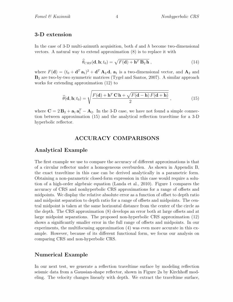
The first example we use to compare the accuracy of different approximations is thatof a circular reflector under a homogeneous overburden. As shown in Appendix B,the exact traveltime in this case can be derived analytically in a parametric form.Obtaining a non-parametric closed-form expression in this case would require a solu-tion of a high-order algebraic equation (Landa et al., 2010). Figure 1 compares theaccuracy of CRS and nonhyperbolic CRS approximations for a range of offsets andmidpoints. We display the relative absolute error as a function of offset to depth ratioand midpoint separation to depth ratio for a range of offsets and midpoints. The cen-tral midpoint is taken at the same horizontal distance from the center of the circle asthe depth. The CRS approximation (8) develops an error both at large offsets and atlarge midpoint separations. The proposed non-hyperbolic CRS approximation (12)shows a significantly smaller error in the full range of offsets and midpoints. In ourexperiments, the multifocusing approximation (4) was even more accurate in this ex-ample. However, because of its different functional form, we focus our analysis oncomparing CRS and non-hyperbolic CRS.

Numerical Example

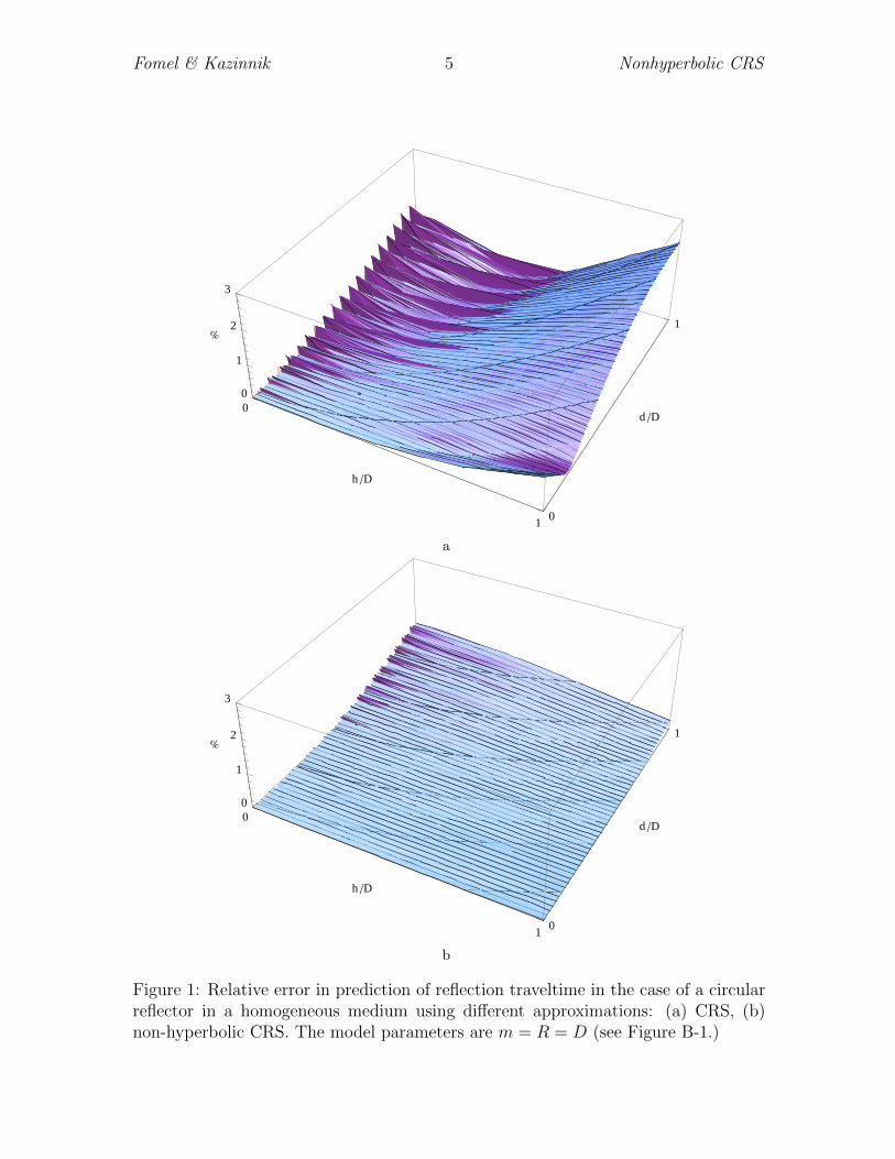
In our next test, we generate a reflection traveltime surface by modeling reflectionseismic data from a Gaussian-shape reflector, shown in Figure 2a by Kirchhoff mod-eling. The velocity changes linearly with depth. We extract the traveltime surface,


0

1

h �D

0

1

d �D

0

1

2

3

%

a

0

1

h �D

0

1

d �D

0

1

2

3

%

b

Figure 1: Relative error in prediction of reflection traveltime in the case of a circularreflector in a homogeneous medium using different approximations: (a) CRS, (b)non-hyperbolic CRS. The model parameters are m = R = D (see Figure B-1.)


a

b

Figure 2: (a) Synthetic velocity model with a Gaussian-shape reflector. (b) Modeledreflection traveltime.


a

b

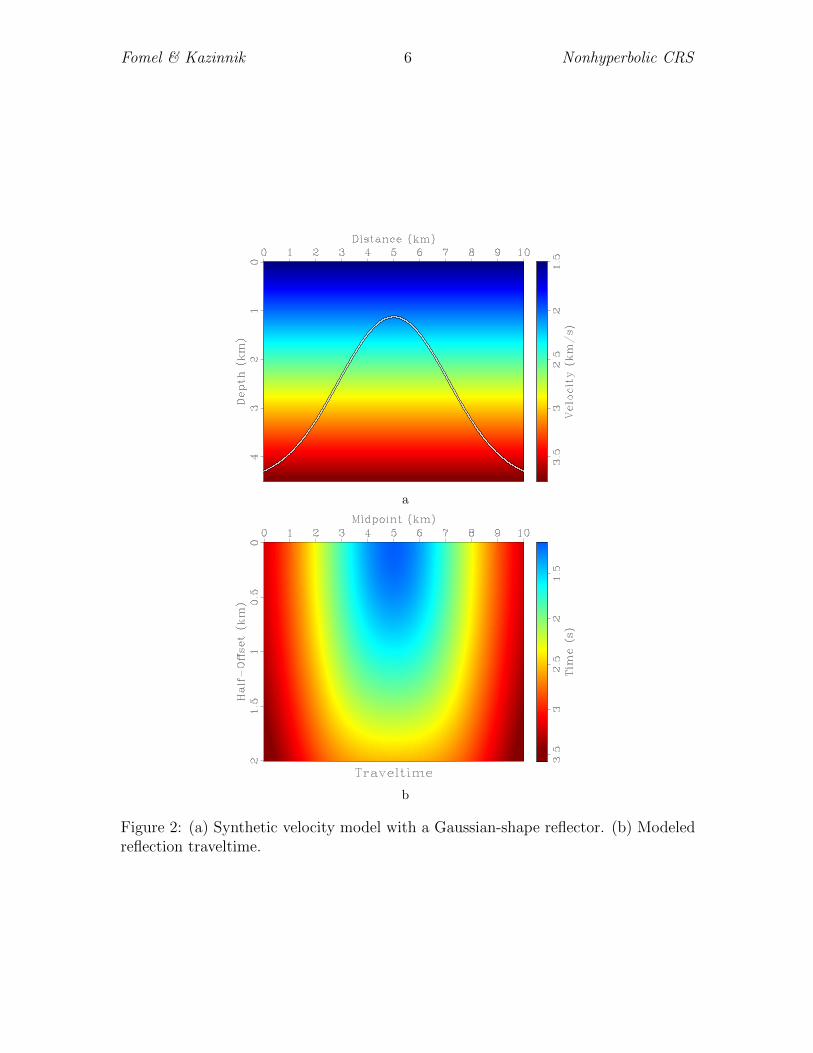
Figure 3: Absolute error of (a) CRS approximation, (b) nonhyperbolic CRS approx-imation. The reference midpoint is at 4 km.


a

b

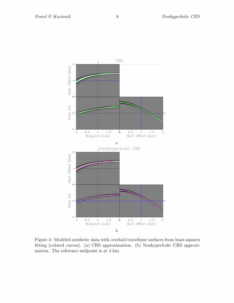
Figure 4: Modeled synthetic data with overlaid traveltime surfaces from least-squaresfitting (colored curves). (a) CRS approximation. (b) Nonhyperbolic CRS approxi-mation. The reference midpoint is at 4 km.


shown in Figure 2b, and fit it with different approximations by non-linear least-squaresoptimization.

Our method for fitting the multivariate time-correction function θ(d, h; t0, a) (ei-ther CRS or nonhyperbolic CRS) to a given experimental time data t(d, h) by findingoptimal parameters set a is a minimization approach, defined as follows:

minaf(a) , (16)

where f is the squared-error sum:

f(a) =1

2

∑d

∑h

|θ(d, h; t0, a)− t(d, h)|2 . (17)

The gradient of the objective function is defined by

∂f

∂ai=∑d

∑h

[θ(d, h; t0, a)− t(d, h)

] ∂θ

∂ai. (18)

The partial derivatives of θ are continuous functions. Therefore, classical minimiza-tion methods, such as the Gauss-Newton iteration, can be employed for finding alocal minimum of f(a) (Bjorck, 1996). In the case of CRS, the solution is uniquebecause of the linear dependence of θ2 on parameters.

The absolute error of CRS and nonhyperbolic CRS approximations, for a rangeof offsets and midpoints, is plotted in Figure 3. The nonhyperbolic CRS error issignificantly smaller for a wide range of offsets and midpoints, which extends theapplicability of the approximation. To effect of different approximations is shownadditionally in Figure 4, which displays the modeled synthetic data with overlaidCRS and nonhyperbolic CRS approximations. The average relative error in differentapproximations, for the selected range of offsets and midpoints, is 1.24 % for the caseof CRS and 0.41 % for the case of nonhyperbolic CRS. The average absolute erroris 25 ms for the case of nonhyperbolic CRS and 8 ms for the case of nonhyperbolicCRS.

CONCLUSIONS

We have presented the non-hyperbolic common reflection surface, a new approxi-mation for prestack reflection traveltimes. Non-hyperbolic CRS uses the same setof parameters as the hyperbolic CRS but in a different functional form, which canmake the approximation significantly more accurate in a large range of offsets andmidpoints. The proposed approximation is derived from the analytical expression ofthe reflection traveltime in the case of a hyperbolic reflector in a constant velocitymedium.

Why use a hyperbolic reflector? A special property of this reflector is that itreduces to a plane reflector or a point diffractor with a special choice of parameters.


(z0 = 0 or α = π/2 respectively). Thus, it encompasses two particularly importantspecial cases.

Numerical experiments show that the new approximation can be significantly moreaccurate than the conventional hyperbolic CRS while using essentially the same setof parameters. The multifocusing approximation can be even more accurate but usesa different set of parameters, which makes it more difficult to extend it to 3-D.

ACKNOWLEDGMENTS

The first author is grateful to Emil Blias, Evgeny Landa, Tijmen Jan Moser, AlexeyStovas, and Martin Tygel for inspiring discussions.

This publication is authorized by the Director, Bureau of Economic Geology, TheUniversity of Texas at Austin.

APENDIX A: HYPERBOLIC REFLECTOR

In this appendix, we reproduce the derivation of an analytical expression for reflec-tion traveltime from a hyperbolic reflector in a homogeneous velocity model (Fomeland Stovas, 2010). Similar derivations apply to an elliptic reflector and were usedpreviously in the theory of offset continuation (Stovas and Fomel, 1996; Fomel, 2003).

Consider the source point s and the receiver point r at the surface z = 0 above a2-D constant-velocity medium and a hyperbolic reflector defined by the equation

z(x) =√z20 + x2 tan2 α . (A-1)

The reflection traveltime as a function of the reflection point location y is

t =

√(s− y)2 + z2(y) +

√(r − y)2 + z2(y)

V. (A-2)

According to Fermat’s principle, the traveltime should be stationary with respect tothe reflection point y:

0 =∂T

∂y=

y − s+ y tan2 α

V√

(s− y)2 + z20 + y2 tan2 α

+y − r + y tan2 α

V√

(r − y)2 + z20 + y2 tan2 α. (A-3)

Putting two terms in equation (A-3) on the different sides of the equation, squar-ing them, and reducing their difference to a common denominator, we arrive at thefollowing quadratic equation with respect to y:

y2 (s+ r) tan2 α − 2 y(s r sin2 α− z20

)− z20 (s+ r) cos2 α = 0 . (A-4)


Only one of the two branches of the solution

y =z20 (s+ r) cos2 α

z20 − s r sin2 α +√

(z20 + s2 sin2 α) (z20 + r2 sin2 α)

has physical meaning. Substituting this solution into equation (A-2), we obtain, aftera number of algebraic simplifications,

t2 =2z20 + s2 + r2 − 2 s r cos2 α

V 2

+2√

(z20 + s2 sin2 α) (z20 + r2 sin2 α)

V 2. (A-5)

Making the variable change in equation (A-5) from s and r to midpoint and half-offsetcoordinates m and h according to s = m− h = m0 + d− h, r = m+ h = m0 + d+ h,we transform this equation to form (12), where the following correspondence betweenparameters is applied:

z20 =t20 a2

(a21 + a2) (a21 + b2), (A-6)

m0 =t0 a1a21 + a2

, (A-7)

sin2 α =a21 + a2a21 + b2

, (A-8)

V 2 =4

a21 + b2. (A-9)

The inverse relationships are given by

t0 =2√m2

0 sin2 α + z20V

, (A-10)

a1 =2m0 sin2 α

V√m2

0 sin2 α + z20, (A-11)

a2 =4 z20 sin2 α

V 2(m2

0 sin2 α + z20) , (A-12)

b2 =4(m2

0 sin2 α cos2 α + z20)

V 2(m2

0 sin2 α + z20) . (A-13)

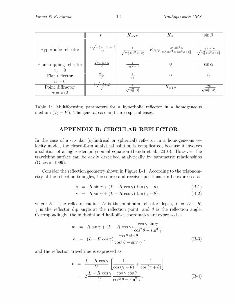
The connection with the multifocusing parameters is summarized in Table 1 forthe general case and three special cases (a plane dipping reflector, a flat reflector, anda point diffractor). The first two special cases turn the nonhyperbolic CRS equationinto the hyperbolic form (8). The last case turns it into the double-square-rootform (13).


t0 KNIP KN sin β

Hyperbolic reflector2√m2

0 sin2 α+z20V

1√m2

0 sin2 α+z20KNIP

z20 sin2 α

m20 sin2 α cos2 α+z20

m0 sin2 α√m2

0 sin2 α+z20

Plane dipping reflectorz0 = 0

2m0 sinαV

1m0 sinα

0 sinα

Flat reflectorα = 0

2 z0V

1z0

0 0

Point diffractorα = π/2

2√m2

0+z20

V1√

m20+z

20

KNIPm0√m2

0+z20

Table 1: Multifocusing parameters for a hyperbolic reflector in a homogeneousmedium (V0 = V ). The general case and three special cases.

APPENDIX B: CIRCULAR REFLECTOR

In the case of a circular (cylindrical or spherical) reflector in a homogeneous ve-locity model, the closed-form analytical solution is complicated, because it involvesa solution of a high-order polynomial equation (Landa et al., 2010). However, thetraveltime surface can be easily described analytically by parametric relationships(Glaeser, 1999).

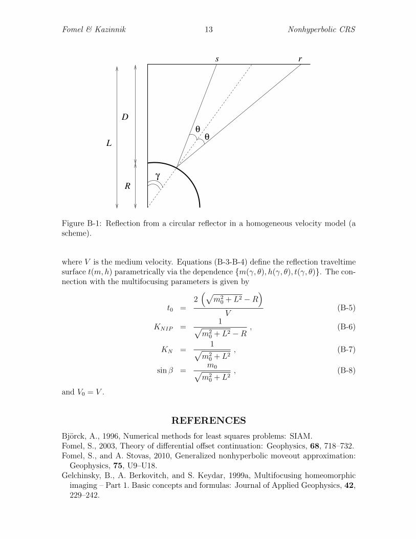
Consider the reflection geometry shown in Figure B-1. According to the trigonom-etry of the reflection triangles, the source and receiver positions can be expressed as

s = R sin γ + (L−R cos γ) tan (γ − θ) , (B-1)

r = R sin γ + (L−R cos γ) tan (γ + θ) , (B-2)

where R is the reflector radius, D is the minimum reflector depth, L = D + R,γ is the reflector dip angle at the reflection point, and θ is the reflection angle.Correspondingly, the midpoint and half-offset coordinates are expressed as

m = R sin γ + (L−R cos γ)cos γ sin γ

cos2 θ − sin2 γ,

h = (L−R cos γ)cos θ sin θ

cos2 θ − sin2 γ, (B-3)

and the reflection traveltime is expressed as

t =L−R cos γ

V

[1

cos (γ − θ)+

1

cos (γ + θ)

]= 2

L−R cos γ

V

cos γ cos θ

cos2 θ − sin2 γ, (B-4)


s r

R

D

γ

Lθ

θ

Figure B-1: Reflection from a circular reflector in a homogeneous velocity model (ascheme).

where V is the medium velocity. Equations (B-3-B-4) define the reflection traveltimesurface t(m,h) parametrically via the dependence {m(γ, θ), h(γ, θ), t(γ, θ)}. The con-nection with the multifocusing parameters is given by

t0 =2(√

m20 + L2 −R

)V

(B-5)

KNIP =1√

m20 + L2 −R

, (B-6)

KN =1√

m20 + L2

, (B-7)

sin β =m0√m2

0 + L2, (B-8)

and V0 = V .

REFERENCES

Bjorck, A., 1996, Numerical methods for least squares problems: SIAM.Fomel, S., 2003, Theory of differential offset continuation: Geophysics, 68, 718–732.Fomel, S., and A. Stovas, 2010, Generalized nonhyperbolic moveout approximation:

Geophysics, 75, U9–U18.Gelchinsky, B., A. Berkovitch, and S. Keydar, 1999a, Multifocusing homeomorphic

imaging – Part 1. Basic concepts and formulas: Journal of Applied Geophysics, 42,229–242.


——–, 1999b, Multifocusing homeomorphic imaging – Part 2. multifold data set andmultifocusing: Journal of Applied Geophysics, 42, 243–260.

Gierse, G., J. Pruessmann, and R. Coman, 2006, CRS strategies for solving severestatic and imaging issues in seismic data from Saudi Arabia: Geophysical Prospect-ing, 54, 709–719.

Glaeser, G., 1999, Reflections on spheres and cylinders of revolution: Journal forGeometry and Graphics, 3, 121–139.

Gurevich, B., S. Keydar, and E. Landa, 2002, Multifocusing imaging over an irregulartopography: Geophysics, 67, 639–643.

Heilmann, Z., J. Mann, and I. Koglin, 2006, CRS-stack-based seismic imaging con-sidering top-surface topography: Geophysical Prospecting, 54, 681–695.

Hoecht, G., P. Ricarte, S. Bergler, and E. Landa, 2009, Operator-oriented CRS in-terpolation: Geophysical Prospecting, 57, 957–979.

Jager, R., J. Mann, G. Hocht, and P. Hubral, 2001, Common-reflection-surface stack:Image and attributes: Geophysics, 66, 97–109.

Landa, E., B. Gurevich, S. Keydar, and P. Trachtman, 1999, Application of multifo-cusing method for subsurface imaging: Journal of Applied Geophysics, 42, 283–300.

Landa, E., S. Keydar, and T. J. Moser, 2010, Multifocusing revisited – Inhomogeneousmedia and curved interfaces: Geophysical Prospecting, 58, 925–938.

Menyoli, E., D. Gajewski, and C. Hubscher, 2004, Imaging of complex basin structureswith the common reflection surface (CRS) stack method: Geophysical JournalInternational, 157, 1206–1216.

Moser, T. J., and E. Landa, 2009, Multifocusing revisited – inhomogeneous mediaand curved interfaces: Presented at the 71st Mtg., Eur. Assn. Geosci. Eng.

Stovas, A. M., and S. B. Fomel, 1996, Kinematically equivalent integral DMO oper-ators: Russian Geology and Geophysics, 37, 102–113.

Tygel, M., and L. T. Santos, 2007, Quadratic normal moveouts of symmetric reflec-tions in elastic media: A quick tutorial: Studia Geophysica et Geodaetica, 51,185–206.

Tygel, M., L. T. Santos, and J. Schleicher, 1999, Multifocus moveout revisited: deriva-tions and alternative expressions: Journal of Applied Geophysics, 42, 319–331.

Yilmaz, O., 2000, Seismic data analysis: Soc. of Expl. Geophys.

Documents

Non-hyperbolic common re ection surfacea - ahay.org · Non-hyperbolic common re ection surfacea aPublished in Geophysical Prospecting, 61, 21-27 (2013) Sergey Fomel and Roman Kazinniky