i

Non-linear Analysis of Stall Flutter Based on the ONERA Aerodynamic Model

Aerospace Engineering Report 0205

Jeremy Beedy and George Barakos

Department of Aerospace Engineering

University of Glasgow

Glasgow G12 8QQ

United Kingdom

July 2002

ii

Contents

Nomenclature iv

1. Introduction 1

1.1.Background 1

1.2. Literature survey 3

1.2.1. Aeroelasticity 3

1.2.2. CFD methods 5

1.2.3. Unsteady aerodynamics 6

1.2.4. Dynamic stall 8

1.3. Objectives 9

1.4. Report outline 9

2. Aeroelastic model 11

2.1. Aerodynamic model 11

2.1.1. Harmonic decomposition of aerodynamic loads 12

2.1.2. Harmonic decomposition of the non-linear part 14

2.2. Flutter calculation 17

2.3. Combined structural-aerodynamics equations. Flutter equations 22

3. Results 26

4. Conclusions and suggestions for future work 28

References 30

Appendix 1. The symmetric part of the aerodynamic curves 34

Appendix 2. The Newton-Raphson method 35

Appendix 3. The Levenberg-Marquardt method 36

Appendix 4. Linear Aerodynamic Coefficients 39

Figures 41

Tables 47

Guide to Computer Programs 50

iii

List of Figures

Figure Description

Fig.1.1 Cantilever wing of uniform cross section.

Fig.1.2 Variation of the lift coefficient (CL) with the angle of attack.

Fig.1.3 Two degree of freedom representation for an aerofoil.

Fig.2.1 Definition of the variables in pitching and plunging motion.

Fig.2.2 Single break-point approximation of the deviation −Cz.

Fig.2.3 Example of oscillation over the stall angle.

Fig.2.4 Change of axis from 1/4 chord to 1/2 chord.

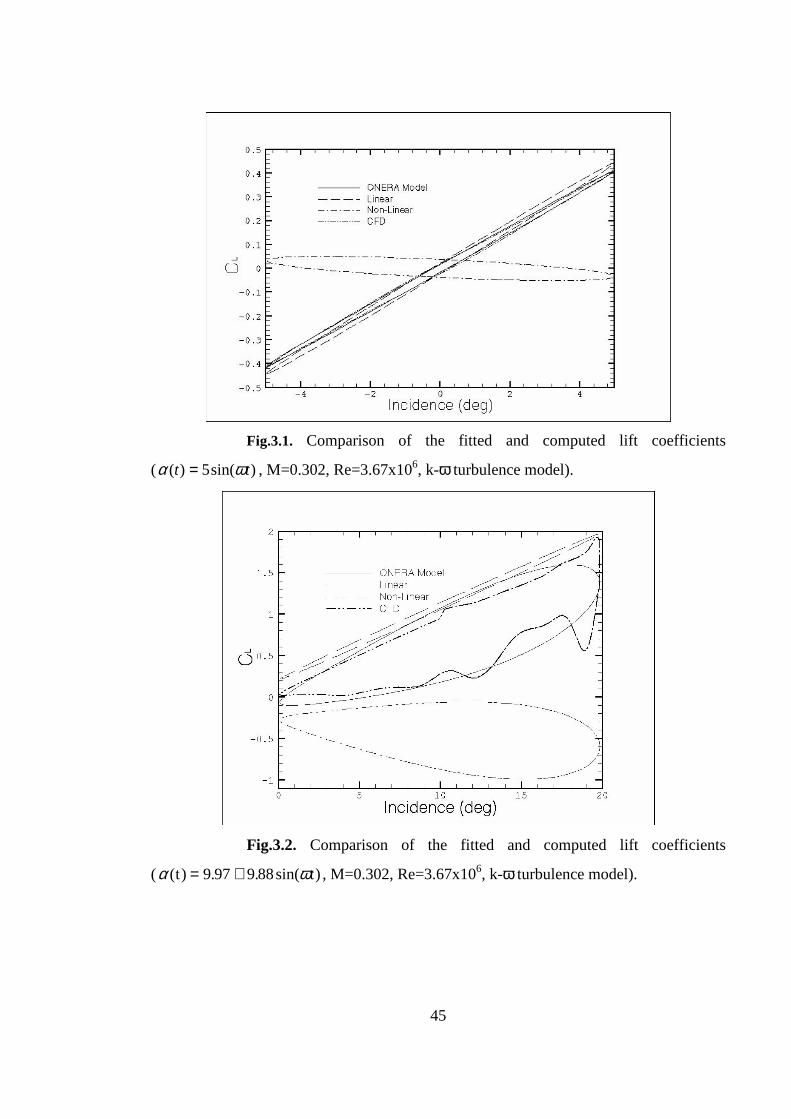
Fig.3.1 Comparison of the fitted and computed lift coefficients ( )sin(5)( tt ωα = ,

M=0.302, Re=3.67x106, k-ω turbulence model).

Fig.3.2 Comparison of the fitted and computed lift coefficients

(α ω( ) . . sin( )t t= +9 97 988 , M=0.302, Re=3.67x106, k-ω turbulence model).

Fig.3.3 Flutter velocity and frequency prediction ( ( ) ( )tt ωα sin88.997.9 += ,

M=0.302, Re=3.67x106, k-ω turbulence model).

iv

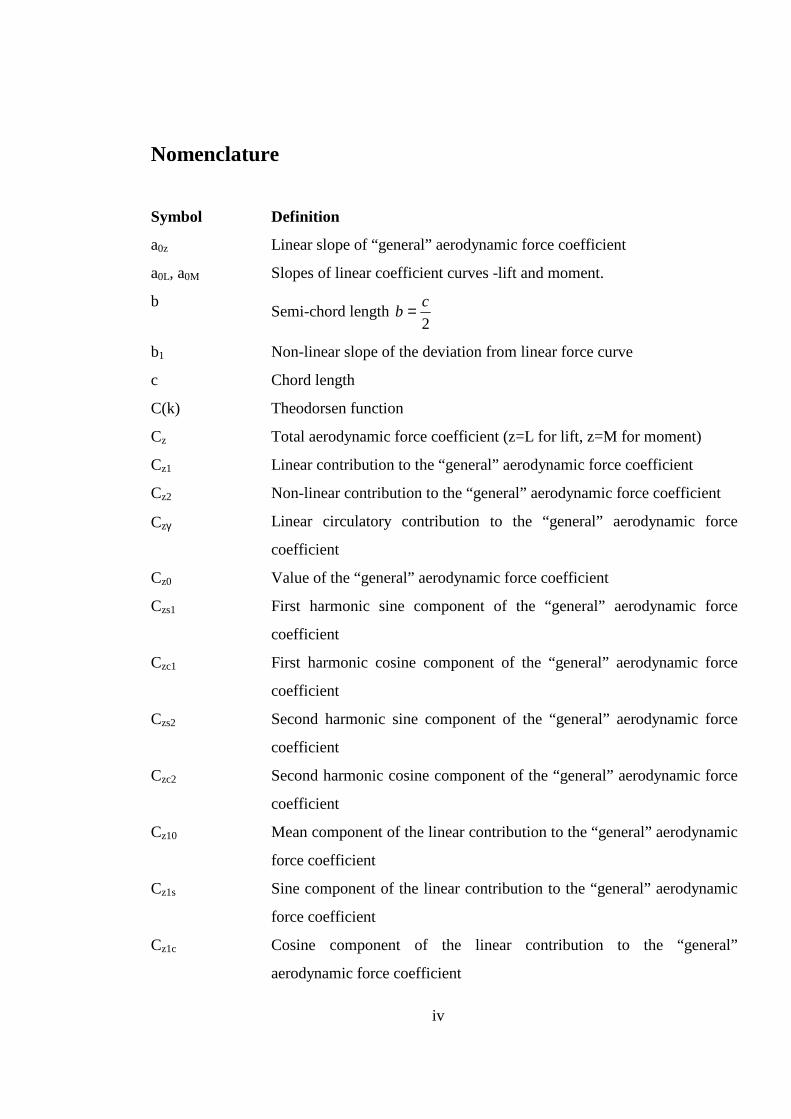
Nomenclature

Symbol Definition

a0z Linear slope of “general” aerodynamic force coefficient

a0L, a0M Slopes of linear coefficient curves -lift and moment.

b Semi-chord length

2

cb =

b1 Non-linear slope of the deviation from linear force curve

c Chord length

C(k) Theodorsen function

Cz Total aerodynamic force coefficient (z=L for lift, z=M for moment)

Cz1 Linear contribution to the “general” aerodynamic force coefficient

Cz2 Non-linear contribution to the “general” aerodynamic force coefficient

Czγ Linear circulatory contribution to the “general” aerodynamic force

coefficient

Cz0 Value of the “general” aerodynamic force coefficient

Czs1 First harmonic sine component of the “general” aerodynamic force

coefficient

Czc1 First harmonic cosine component of the “general” aerodynamic force

coefficient

Czs2 Second harmonic sine component of the “general” aerodynamic force

coefficient

Czc2 Second harmonic cosine component of the “general” aerodynamic force

coefficient

Cz10 Mean component of the linear contribution to the “general” aerodynamic

force coefficient

Cz1s Sine component of the linear contribution to the “general” aerodynamic

force coefficient

Cz1c Cosine component of the linear contribution to the “general”

aerodynamic force coefficient

v

Cz20 Mean harmonic component of the non-linear contribution to the

“general” aerodynamic force coefficient

Cz2s1 Sine first harmonic component of the non-linear contribution to the

“general” aerodynamic force coefficient

Cz2c1 Cosine first harmonic component of the non-linear contribution to the

“general” aerodynamic force coefficient

Cz2s2 Sine second harmonic component of the non-linear contribution to the

“general” aerodynamic force coefficient

Cz2c2 Cosine second harmonic component of the non-linear contribution to the

“general” aerodynamic force coefficient

Czγ0 Mean component of the linear circulatory contribution to the “general”

aerodynamic force coefficient

Czγs Sine component of the linear circulatory contribution to the “general”

aerodynamic force coefficient

Czγc Cosine component of the linear circulatory contribution to the “general”

aerodynamic force coefficient

e Distance from elastic axis to mid-chord

Total energy of the fluid per unit volume

F(k) Real part of the Theodorsen function

FKleb Klebanoff’s intermittency function

G(k) Imaginary part of the Theodorsen function

h Tip deflection about ¼ chord

h0 Mean component of the ¼ chord deflection

hs Sine component of the ¼ chord deflection

hc Cosine component of the ¼ chord deflection

Hν Source term associated with turbulence model

i Internal energy

Ia Mass moment of inertia per unit length

k Reduced frequency k

b

U= ⋅ω

ka Torsional reduced frequency

vi

Ka Torsional stiffness per unit length

Kh Bending stiffness per unit length

[K] Stiffness matrix

kij Components of the stiffness matrix

l Wing length

lmix Mixing length

L Lift

M Total mass per unit length

Ma Pitching moment

[M] Mass matrix

M ij Components of the mass matrix

n Number of modal shapes

p Pressure

qi i-th modal amplitude

qio Mean component of the i-th modal amplitude

qis Sine component of the i-th modal amplitude

qic Cosine component of the i-th modal amplitude

q Dynamic pressure �

q Heat flux

Qi i-th modal force

Qi0 Mean component of the i-th modal force

Qis Sine component of the i-th modal force

Qic Cosine component of the i-th modal force

r0 Gyration radius

r1, r2, r3 Coefficients of ONERA non-linear aerodynamic differential equations

r10, r12, r20,

r22, r30, r32

Parabolic coefficients of ONERA non-linear aerodynamic equations

S Wing surface area

Sz1, Sz2, Sz3 Coefficients of linear ONERA aerodynamic modes

Sa Static moment of inertia per unit length

t Real time

vii

U Free stream velocity

Udif Maximum value of U.

w Velocity component in the z-direction

Greek symbols Definition

α Angle of attack

α0 Mean component of the angle of attack

αs Sine component of the angle of attack

αc Cosine component of the angle of attack

α1 Stall angle

αv Vibration amplitude of the angle of attack

γi Non-dimensional mode shape

δij Kronecker’s delta

∆Cz Deviation of the non-linear aerodynamic force curve from the linear

approximation

∆Cz0, ∆Czs1,

∆Czc2

First and second harmonic oscillatory amplitudes of the deviation of the

non-linear aerodynamic force curve from the linear approximation

εj Parameter of the j-th beam bending mode shapes

Θ =ωω

h

a

Ratio of bending to torsional frequency

θ Pitch angle about ¼ chord

θ0 Mean component of the pitch angle

θs Sine component of the pitch angle

θc Cosine component of the pitch angle

θR Root angle of attack

κ von Karman constant

λ1, λ2 Coefficients in linear aerodynamic force model

µ Density ratio=

⋅ ⋅M

bπ ρ 2

ξ,ζ Curvilinear coordinates

ρ Free stream density

viii

τ Dimensionless time=

⋅t U

b

φ Non-dimensional phase associated with the angle of attack

Φa Beam torsion mode shape

Φh Beam bending mode shape

ω Real frequency

Magnitude of the vorticity vector

ωa Uncoupled torsion frequency

ωh Uncoupled bending frequency

ω* Under-relaxation parameter

1

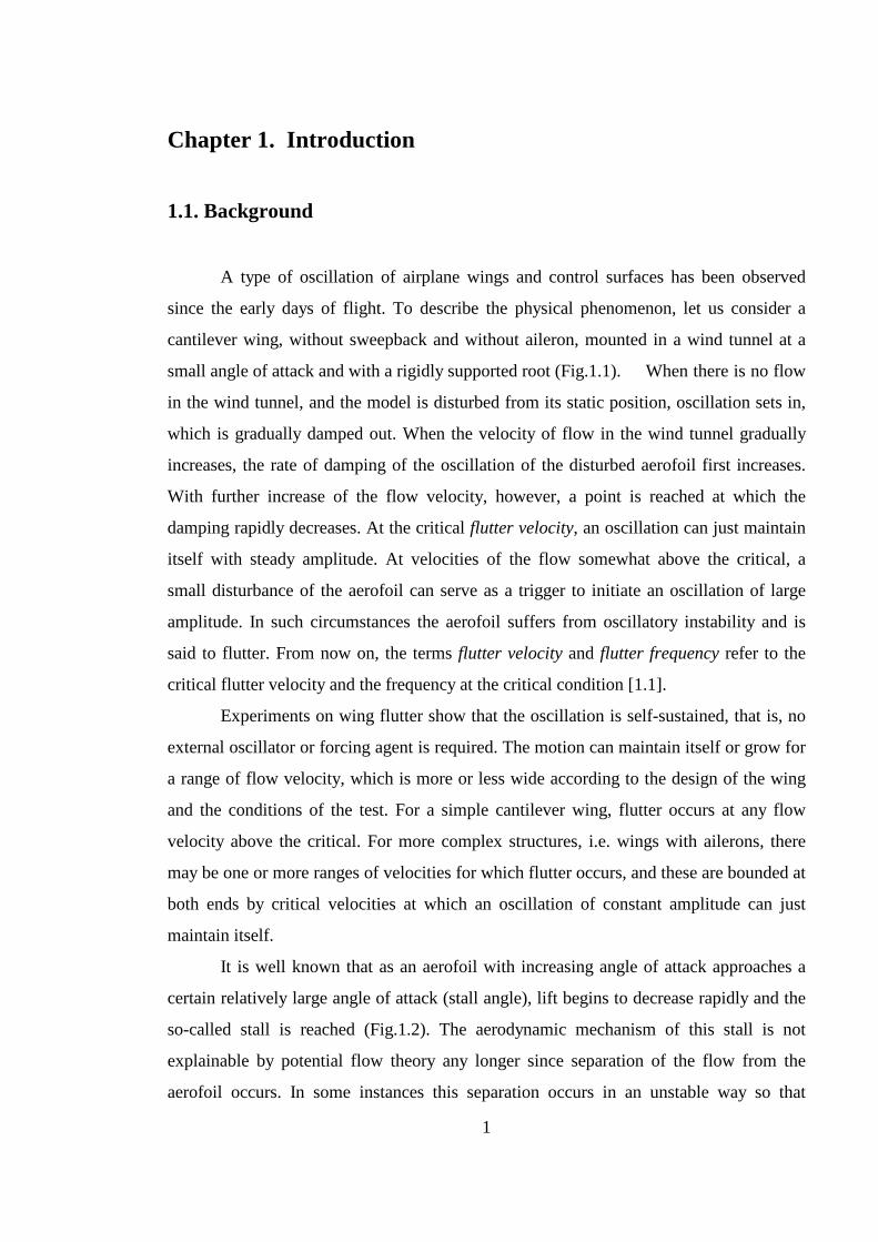
Chapter 1. Introduction

1.1. Background

A type of oscillation of airplane wings and control surfaces has been observed

since the early days of flight. To describe the physical phenomenon, let us consider a

cantilever wing, without sweepback and without aileron, mounted in a wind tunnel at a

small angle of attack and with a rigidly supported root (Fig.1.1). When there is no flow

in the wind tunnel, and the model is disturbed from its static position, oscillation sets in,

which is gradually damped out. When the velocity of flow in the wind tunnel gradually

increases, the rate of damping of the oscillation of the disturbed aerofoil first increases.

With further increase of the flow velocity, however, a point is reached at which the

damping rapidly decreases. At the critical flutter velocity, an oscillation can just maintain

itself with steady amplitude. At velocities of the flow somewhat above the critical, a

small disturbance of the aerofoil can serve as a trigger to initiate an oscillation of large

amplitude. In such circumstances the aerofoil suffers from oscillatory instability and is

said to flutter. From now on, the terms flutter velocity and flutter frequency refer to the

critical flutter velocity and the frequency at the critical condition [1.1].

Experiments on wing flutter show that the oscillation is self-sustained, that is, no

external oscillator or forcing agent is required. The motion can maintain itself or grow for

a range of flow velocity, which is more or less wide according to the design of the wing

and the conditions of the test. For a simple cantilever wing, flutter occurs at any flow

velocity above the critical. For more complex structures, i.e. wings with ailerons, there

may be one or more ranges of velocities for which flutter occurs, and these are bounded at

both ends by critical velocities at which an oscillation of constant amplitude can just

maintain itself.

It is well known that as an aerofoil with increasing angle of attack approaches a

certain relatively large angle of attack (stall angle), lift begins to decrease rapidly and the

so-called stall is reached (Fig.1.2). The aerodynamic mechanism of this stall is not

explainable by potential flow theory any longer since separation of the flow from the

aerofoil occurs. In some instances this separation occurs in an unstable way so that

2

fluctuating conditions ranging from near-potential flow conditions to very turbulent

conditions are obtained. If a body is fluttering and, during part or all of the time of

oscillation the flow is separated, then the flutter phenomenon is called a stall flutter.

Stall flutter is a serious aeroelastic instability for rotating machineries such as

propellers, turbine blades, and compressors, which sometimes have to operate at angles of

attack close to the static stalling angle of the blades. Airplane wings and tails rarely suffer

from stall flutter. However, the trend toward thin wing sections and large wingspan has

increasingly made stall flutter of wings a serious concern for the design of high-speed

aircraft.

Most analysis of aircraft flutter behaviour is traditionally based on small

amplitude, linear theory, particularly with respect to the aerodynamic modelling.

However, if the wing is near the stall region, a non-linear stall flutter limit cycle may

occur at a lower velocity than linear theory suggests. Since some current aircraft are

achieving high angle of attack for manoeuvring, it is of interest to explore this non-linear

stall flutter behaviour and its transition from linear behaviour.

The objective of the present work is to explore analytically the roles of non-linear

aerodynamics in high angle-of-attack stall flutter while attempting to develop a simple

non-linear method of flutter analysis.

The non-linear flutter calculations were carried out solving the Rayleigh-Ritz

formulation using the ONERA model [1.2,1.3] as the basis for the aerodynamics. A

harmonic balance method and a Newton-Raphson solver were applied to the resulting

non-linear equations.

In order to fit some parameters of the ONERA model, a CFD code was used to

calculate the aerodynamic coefficients of an aerofoil undergoing oscillatory motion. The

code uses an implicit unfactored method with various turbulence models [1.4]. It

combines Newton sub-iterations and point-by-point Gauss-Seidel sub-relaxations.

3

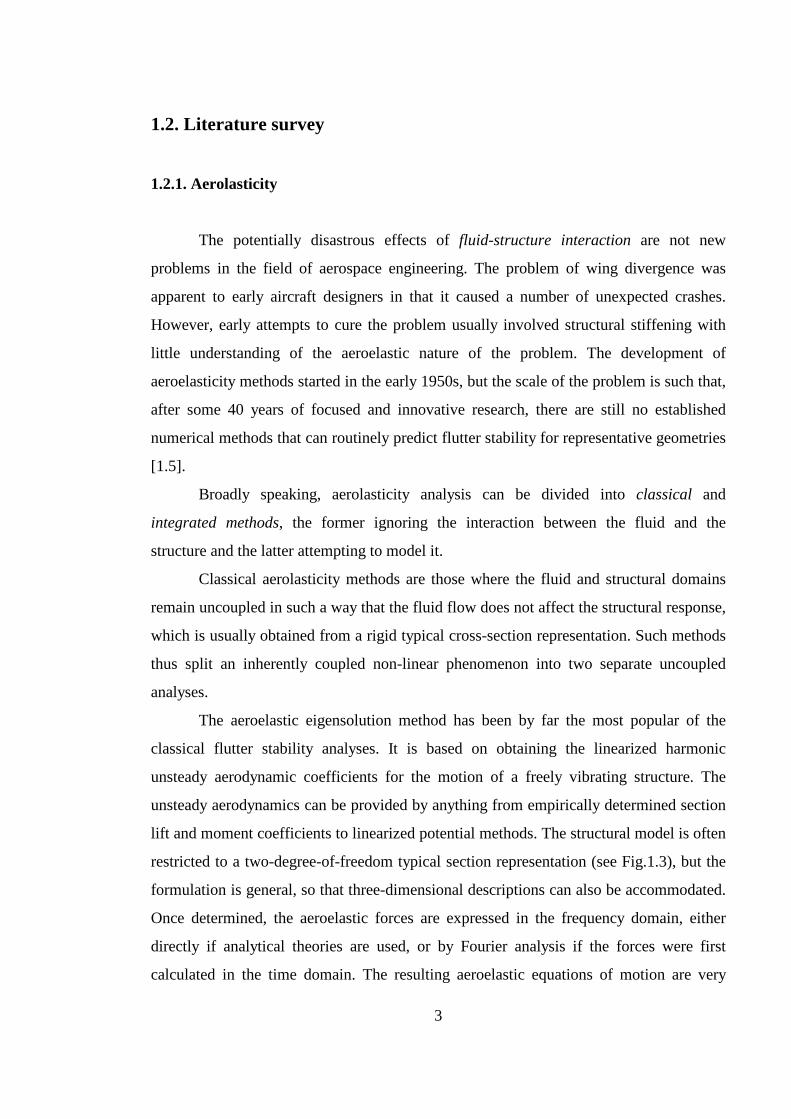
1.2. Literature survey

1.2.1. Aerolasticity

The potentially disastrous effects of fluid-structure interaction are not new

problems in the field of aerospace engineering. The problem of wing divergence was

apparent to early aircraft designers in that it caused a number of unexpected crashes.

However, early attempts to cure the problem usually involved structural stiffening with

little understanding of the aeroelastic nature of the problem. The development of

aeroelasticity methods started in the early 1950s, but the scale of the problem is such that,

after some 40 years of focused and innovative research, there are still no established

numerical methods that can routinely predict flutter stability for representative geometries

[1.5].

Broadly speaking, aerolasticity analysis can be divided into classical and

integrated methods, the former ignoring the interaction between the fluid and the

structure and the latter attempting to model it.

Classical aerolasticity methods are those where the fluid and structural domains

remain uncoupled in such a way that the fluid flow does not affect the structural response,

which is usually obtained from a rigid typical cross-section representation. Such methods

thus split an inherently coupled non-linear phenomenon into two separate uncoupled

analyses.

The aeroelastic eigensolution method has been by far the most popular of the

classical flutter stability analyses. It is based on obtaining the linearized harmonic

unsteady aerodynamic coefficients for the motion of a freely vibrating structure. The

unsteady aerodynamics can be provided by anything from empirically determined section

lift and moment coefficients to linearized potential methods. The structural model is often

restricted to a two-degree-of-freedom typical section representation (see Fig.1.3), but the

formulation is general, so that three-dimensional descriptions can also be accommodated.

Once determined, the aeroelastic forces are expressed in the frequency domain, either

directly if analytical theories are used, or by Fourier analysis if the forces were first

calculated in the time domain. The resulting aeroelastic equations of motion are very

4

similar to the structural equations, the aerodynamic contribution being added to the mass

and/or stiffness matrices. However, these new system matrices may well become a

function of the frequency, in which case the eigenproblem is no longer mathematically

linear. In such situations an approximate solution can be found using iterative techniques.

One of the main disadvantages of the method lies in its simplified representation of the

structural dynamics (usually a lumped parameter model), which allows parametric studies

to be conducted with minimum computational effort.

Tran and Petot [1.2] and Dat and Tran [1.3] of the Office National d’Etudes et de

Recherches Aérospatiales (ONERA) developed, in the 1980´s, a semi-empirical,

unsteady, non-linear model (called the ONERA model) for determining two-dimensional

aerodynamic forces on an aerofoil oscillating in pitch only, which experiences dynamic

stall. It was felt that this model, as amended for pitch and plunge by Peters [1.6] and by

Petot and Dat [1.7], could provide a convenient means of including non-linear stalled

aerodynamic forces into an analytical study of stall flutter.

Dunn and Dugundji [1.8] developed a simple analytic method to include non-

linear structural and aerodynamic effects into a stall flutter analysis, using the ONERA

model for the aerodynamics. Experimental data were obtained on a set of aeroelastically

tailored wings with varying amounts of bending-torsion coupling. The analysis predicted

reasonably almost all the observed, experimental, non-linear stalled phenomena on the

wings tested.

The flutter behaviour of rotor blades has also been investigated. Chopra and

Dugundji [1.9] gave an analysis of the non-linear aeroelastic behaviour and its transition

from linear behaviour, but dealing only with geometrical non-linearities of the rigid blade.

Tang and Dowell [1.10] have introduced both structural non-linearities and

dynamic stall in their investigation of stall limit cycles and chaotic motion of flexible, non

rotating blades. In their work the structural non-linearities were approximated by the

moderate deflection equations developed by Hodges and Dowell [1.11], and the dynamic

stall was represented by the ONERA model. Kim and Dugundji [1.12] incorporated the

structural effects into a non-linear, large amplitude flutter limit cycle analysis of rotating

hingeless composite blades using the ONERA model.

5

1.2.2. CFD methods

With dramatic increases in computing power and advances in computational fluid

dynamics (CFD) methods, it is now possible to obtain solutions for both inviscid

(hyperbolic Euler equations) and viscous (parabolic Navier-Stokes equations) steady

flows, including a reasonable representation of viscous losses. The usual approach is to

use time integration, starting from known initial conditions. Unsteady flows are much

more complex in nature because of temporal variations, but representative solutions can

still be obtained if the time-dependent terms are discretized in a time-accurate fashion.

Over the last two decades, time domain solutions have progressed through full-potential,

linearized-Euler, Euler and, most recently, Reynolds-averaged Navier-Stokes equations.

Two distinct methods have been adopted to discretize the fluid domain. The first

one, known as finite-difference, is based on the differential form of the governing

equations. The physical grid on which the calculation is to be performed is transformed to

a rectangular computational grid with equal spacings in each direction, onto which the

equations are discretized. The second method, known as finite-volume, uses the integral

form of the governing equations, which are discretized as fluxes through control volumes

of known shape but arbitrary size. Further differences between the CFD methods lie in the

integration schemes adopted (explicit or implicit) for solving the discretized equations

(cell vertex or cell centred schemes), the meshing strategy used (structured- O, C, or H

meshes; unstructured- adaptive, dynamic meshes) and the implementation of the

boundary conditions (non-reflecting, periodic, moving boundaries)[1.5].

One of the major problems associated with three dimensional unsteady flow

modelling is the amount of CPU time required to obtain fully converged solutions. The

modelling of turbulence is probably one of the most significant challenges to the accuracy

of modern CFD methods. For the foreseeable future, it is impractical to contemplate a

direct application of the Navier-Stokes equations to turbulence as an unrealistically fine

mesh would be required to capture the smallest eddies, an approximate size of which

being provided by the Kolmogorov scale. Therefore, turbulence can only be represented

using simplified models which are usually based on equivalent local turbulent viscosities

given by the averaged effect of the eddies at some point in the flow. There is a hierarchy

6

of such methods which range from the fully empirical mixing length model (zero-

equation eddy viscosity model: Baldwin & Lomax[1.13]), one-equation k-l models

(Cebeci & Smith [1.14]; Johnson & King [1.15]; Baldwin & Barth [1.16]), two-equations

k-ε models (Jones & Launder [1.17]), to the Reynolds stress model with six equations in

2D and nine equations in 3D.

1.2.3. Unsteady aerodynamics

Currently, the most accurate aerodynamic models are computational fluid dynamic

solutions to the governing equations. These CFD-based approaches are often considered

to be the salvation of the aeroelastician; however, in many situations, a time-marching

aeroelastic analysis using a CFD method is very computationally expensive for routine

design purposes or parametric studies.

There exists, therefore, a need to develop “ rational” prediction methods so that

expensive and time-consuming development testing can be minimized. There are broadly

two different approaches available to achieve this goal, i.e. viscous-inviscid interaction

methods and Navier-Stokes methods. The former method couples inviscid flows with

boundary layer flows (Abdel-Rahim et al. [1.18], Jang et al. [1.19], Cebeci et al. [1.20]),

whereas the latter relies on the solution of the full viscous flow equations.

Clarkson, Ekaterinaris and Platzer [1.21] attempted the analysis of aerofoil stall

flutter by applying a Navier-Stokes flow solver to the problem of low subsonic flow,

M=0.3, over an oscillating NACA-0012 aerofoil in the light stall regime. The flow was

assumed fully turbulent, and the Baldwin-Lomax, the algebraic RNG-based model and

the half-equation Johnson-King turbulence models were used. It was found that none of

these models was capable of reproducing the hysteresis loops measured by McCroskey

[1.22].

As is well known, modelling of the turbulence flow behaviour is an important

issue in computational aerodynamics. The flow over an oscillating blade is often

massively separated and involves multiple length scales. For the computation of these

flows, application of algebraic turbulence models, such as the Cebeci-Smith, the

Baldwin-Lomax, or the Johnson-King model, becomes very complicated and also

7

ambiguous. The source of this ambiguity comes from the difficulty in defining

characteristic length scales, such as boundary layer thickness. An extensive investigation

of the ability of these simple models as well as the recently developed Baldwin-Barth and

Spalart-Almaras [1.23] one-equation models to predict unsteady separated flows has been

conducted [1.24]. The one-equation models have shown superior behaviour compared to

algebraic models.

Two-equation models, such as the k-ε and the k-ω models, have also been used to

compute steady and unsteady aerofoil flows [1.25]. It appears that the k-ω model provides

some improvements over the one-equation models. The k-ε model, on the other hand,

does not predict well the adverse pressure gradient separated flow regions.

Numerical investigations [1.26] of aerofoil flows showed that the effect of the

leading edge transitional flow region is of primary importance to the overall development

of the suction side viscous flow region. Laminar/transitional separation bubbles form near

the aerofoil leading edge for angles of incidence as low as 6 deg and significantly alter the

suction side pressure distribution and the boundary layer formation.

Ekaterinaris and Platzer [1.27] show that it is important to take into account the

leading edge transitional flow not only for the lower Reynolds number regime but also for

the high Reynolds number in order to predict stall flutter. For the high Reynolds number

regime, transition is expected to occur very close to the leading edge after the adverse

pressure gradient region is encountered. The extent of the transition region and the

separation bubble is also expected to be very small. Their results for an oscillating

aerofoil show that modelling of the transitional flow near the leading edge decisively

changes the character of the pitching moment hysteresis loop. Whereas the fully turbulent

calculations produce only counter clockwise moment loops, the transitional calculations

produce clockwise loops. Their finding is very important since it is well known (see

[1.28]) that single-degree-of-freedom stall flutter in pitch occurs as soon as the area

enclosed by the clockwise moment loop exceeds the area enclosed by the counter

clockwise loop.

8

1.2.4. Dynamic Stall

The dynamic stall process has been under investigation for about three decades,

and significant progress has been made towards understanding the physical processes

associated with the rapidly pitching of an aerofoil beyond its static stall angle of attack.

In the 70’s the study of unsteady turbulent flows was dominated by the work of

Stuart, Telionis, Wirz, McCroskey and Shen. The above efforts are mainly experimental

studies and attempts to derive analytical solutions for unsteady boundary layers. In the

80’s the rapid progress of computer technology allowed researchers to simulate unsteady

flows using numerical techniques. The reviews of McCroskey [1.29], Carr [1.30] and

Visbal [1.31] provide good descriptions of the dynamic stall processes. In the 90’s the

effect of turbulence on dynamic stall has been the subject of extensive experimental

[1.32] and numerical studies [1.33].

The earliest computational investigations of dynamic stall appeared in 70s and

early 80s with indicative efforts by Mehta [1.34] and Gulcat [1.35]. In the middle 80s, the

algorithm by Wu [1.36, 1.37] for incompressible flow provided results consistent with

experimental data. Tuncer [1.38] extended the model for high Reynolds number flows,

obtaining accurate and inexpensive results.

Compressibility effects have been addressed during the past few years, with high

Reynolds number compressible flow solutions appearing infrequently. The time delay

between the appearance of incompressible and compressible Navier-Stokes solutions

primarily represents increased computational requirements. Compressibility adds an

additional differential equation (for energy) to the system of equations to be solved.

Furthermore, the solution must account for sharp flow-field gradients and include

thermodynamic features such as shock waves.

High Reynolds number flows not only increase the computer demand but also

require turbulence modelling. To date such modelling seems as much an art as a science.

Examination of the available literature reveals that detailed investigations of dynamic

stall including high Mach and Reynolds number effects as well as lower pitch rates and

more complex aerofoils, are rare. High pitch rates generally produce more straight-

forward, vortex-dominated flows where turbulence is less pronounced. Low pitch rate

9

flow fields are usually more difficult to compute. Finally, complex aerofoils require

complex grid generators and exhibit edges, such as truncated trailing edges, which can

produce numerical difficulties.

1.3. Objectives

The objective of the project is to develop a method of analysing flutter in

aerofoils.

The flutter calculations are based on a non-linear model for the aerodynamic part

(ONERA model) and on a linear model for the structural part. The non-linear equation of

the ONERA model has several parameters, which have to be supplied to the model, for

each case, from either:

i) experimental data, or

ii) CFD simulation.

Several cases are solved using the unsteady Parallel Multi-Block (PMB) CFD

code to calculate the loads on an aerofoil under certain oscillating conditions, and hence

obtaining the lift and moment loops. The solver combines Newton sub-iterations and

point-by-point Gauss-Seidel sub-relaxation. For this study, a k-ω turbulence model is

used. Some cases are solved as fully turbulent problems and others with tripping. The grid

is not very fine, and the time resolution is the minimum possible, in order to simplify the

calculations.

Using the results from the code, and the available experimental data, the

parameters of the ONERA model are fitted. The fitting is done using the Levenberg-

Marquardt method, a non-linear fitting method.

Once the parameters are fitted for every case, the flutter program is run to obtain

the flutter velocity and frequency of the aerofoil.

1.4. Report outline

The report is structured in the following parts:

10

Chapter 2. Aeroelastic model: the ONERA model and the basic calculations for the

flutter are explained here. This is the basis of the flutter program.

Chapter 3. Results: first, the solved cases are described. After that, the results are

presented and discussed.

Chapter 4. Conclusions: the most relevant findings are briefly summarized and

suggestions for the future are made.

Appendices Details of the computer implementation of the model along with description

of the employed numerical methods are given in the appendices.

11

Chapter 2. Aeroelastic model

An aeroelastic model consists of two parts: aerodynamic and structural. Non-

linearities in the structural part can arise from geometry and material while in the

aerodynamic part they can arise from flow separation and stall. In the present work only

aerodynamic non-linearities are considered.

2.1. Aerodynamic model

The ONERA aerodynamic model [2.1] was used in this study in order to solve the

aerodynamic non-linearities. According to this model all airloads can be expressed as the

sum of a linear and non-linear part as:

C C Cz z z= +1 2 (2.1)

The linear part, Cz1, is given by:

C S S S Cz z z z z1 1 2 3= ⋅ + ⋅ + ⋅ +�

��� �

α θ θ γ (2.2)

�

(�

) (�

���

)C C a az z z zγ γλ λ α θ λ α θ+ ⋅ = ⋅ ⋅ + + ⋅ ⋅ +1 1 0 2 0 (2.3)

While the non-linear one, Cz2, is:

��� � �

C r C r C r C r Cz z z z z2 1 2 2 2 2 3+ ⋅ + ⋅ = − ⋅ − ⋅∆ ∆α α (2.4)

In the above equations:

α θ= − ~�

h (Incidence angle, separated into pitching and plunging, see fig.2.1)

(2.5)

( ) ( )~ =b

( ) ( ) ( ) ( )⋅ ⋅⋅= = = ⋅∂∂τ

∂∂τ

τ2

2

U t

b (2.6)

( )⋅ Stands for the first time derivative, and ( )⋅⋅ for the second time derivative. ∆Cz is the

deviation of the non-linear aerodynamic curve from the linear approximation (Fig.2.2).

For this model, z represents a general aerodynamic load, which can be lift (L) or

moment (M), and the parameters of the linear equations are:

12

SL1=3.142 SL2=1.571 SL3=0.0

SM1= -0.786 SM2= -0.589 SM3= -0.786

a0L=6.28 aOM=0.0

λ1=0.15, λ2=0.55 (same for lift and moment calculations)

where a0L and a0M represent the slopes of the linear coefficient curves.

The term CzΚ (circulatory contribution to the linear aerodynamic coefficient)

accounts for the aerodynamic lag due to the formation of flow structures, like vortices.

The total static lift or moment coefficient can be calculated as:

C a Cz z z( ) ( )α α α= ⋅ −0 ∆ (2.7)

where a0z is the slope of the linear aerodynamic curve.

−Cz can be approximated in any convenient way suitable for a particular study.

For this model, a straight segment between discrete points will be used, as in Fig.2.2.

2.1.1. Harmonic decomposition of aerodynamic loads

Now, using the harmonic balance method, the system of differential equations

(expressed in the time domain) is transformed into a system of non-linear algebraic

equations (expressed in the frequency domain). Then it is necessary to write all the

variables involved in the equations of the model as the sum of a mean, sine and cosine

parts. For the pitching angle (θ) and deflection at the quarter chord (h):

θ τ θ θ τ θ τ( ) sin cos= + ⋅ + ⋅0 s ck k (2.8)

h h h k h ks c( ) sin cosτ τ τ= + ⋅ + ⋅0 (2.9)

Here ω represents the real frequency of vibration.

Their derivatives are:

�

cos sinθ θ τ θ τ= ⋅ ⋅ − ⋅ ⋅s ck k k k (2.10)

���

sin cosθ θ τ θ τ= − ⋅ ⋅ − ⋅ ⋅s ck k k k2 2 (2.11)

�

cos sinh h k k h k ks c= ⋅ ⋅ − ⋅ ⋅τ τ (2.12)

���

sin cosh h k k h k ks c= − ⋅ ⋅ − ⋅ ⋅2 2τ τ (2.13)

The effective angle of attack is:

13

α α α τ α τ= + ⋅ + ⋅0 s ck ksin cos (2.14)

or, in a purely sinusoidal form:

α α α τ ξ α α φ= + ⋅ + = + ⋅0 0v vksin( ) sin (2.15)

where α α αv s c= +2 2 (2.16)

φ τ ξ= ⋅ +k (2.17)

ξ αα

= −sin 1 c

v (2.18)

And as the incidence angle can be decomposed into pitching and plunging

(α θ= − ~�h):

α θ0 0= (2.19)

α θs sch

bk= + ⋅ (2.20)

α θc csh

bk= − ⋅ (2.22)

Following the same procedure for CzΚ (circulatory contribution) and its first

derivative results in:

C C C k C kz z z s z cγ γ γ γτ τ= + ⋅ + ⋅0 sin cos (2.23)

�

cos sinC C k k C k kz z s z cγ γ γτ τ= ⋅ ⋅ − ⋅ ⋅ (2.24)

Substituting the equations obtained in that decomposition in eq. (2.3), it yields:

C az zγ θ0 0 0= ⋅ (2.25)

C F k L G k Lz s s cγ = ⋅ − ⋅( ) ( ) (2.26)

C G k L F k Lz c s cγ = ⋅ + ⋅( ) ( ) (2.27)

where:

L a kh

bks z s

cc= ⋅ − ⋅ − ⋅�

��

���0 θ θ (2.28)

L a kh

bkc z c

ss= ⋅ + ⋅ + ⋅�

��

���0 θ θ (2.29)

F kk

k( ) = ⋅ +

+

22 1

2

12 2λ λ

λ (2.30)

14

( )

G kk

k( ) =

⋅ ⋅ −

+

λ λ

λ1 2

12 2

1 (2.31)

In the above, F and G are the real and imaginary parts, respectively, of C(k):

C(k F k i G k) ( ) ( )= + ⋅

C(k) is the approximation to the Theodorsen function C ikik

ik( ) =

⋅ ++

λ λλ

2 1

1

, which

is characteristic of circulation terms, where λ1=0.15, λ2=0.55 and i = −1 .

Using the harmonic decomposition shown in eq. (2.25), (2.26) and (2.27) the

following decomposition can be obtained for the linear part of the aerodynamic

coefficient (Cz1):

Mean component:

C Cz z10 0= γ (2.32)

Sinus component:

C S khb

k S k S k Cz1s z1 cs

z s z c z s= ⋅ ⋅ − ⋅���

��� − ⋅ ⋅ − ⋅ ⋅ +θ θ θ γ

22

23 (2.33)

Cosinus component:

C S khb

k S k S k Cz1c z1 sc

z c z s z c= ⋅ ⋅ − ⋅���

��� − ⋅ ⋅ + ⋅ ⋅ +θ θ θ γ

22

23 (2.34)

2.1.2. Harmonic decomposition of the non-linear part

For the non-linear portion of the ONERA model, the same harmonic

decomposition is used.

Since the aerodynamic curve is modelled by a single break point approximation,

−Cz can be calculated as

∆C bz = ⋅ −1 1( )α α for α>α1 (2.35)

= 0 for α≤α1

where Ι1 is the stall angle and b1 is the slope of the deviation from linear force curve.

To simplify the rest of the calculation the angle of attack (α) is used in the form

where it is purely sinusoidal, then:

15

( )∆C bz v= ⋅ + ⋅ −1 0 1α α φ αsin (2.36)

Using the decomposition in mean, sine and cosine terms:

∆ ∆ ∆ ∆C C C Cz z zs zc= + ⋅ + ⋅0 1 2 2sin cosφ φ (2.37)

Only one sine term is included above due to the single-valued α function assumed

for ∆Cz.

Substituting in the above using (2.36) and Fourier transformation gives:

( )∆C b dz v0 1 0 1

1

21= ⋅ ⋅ + ⋅ −�π

α α φ α φφ

πsin

/

(2.38)

( )∆C b dzs v1 1 0 1

1

22= ⋅ ⋅ + ⋅ − ⋅�π

α α φ α φ φφ

πsin sin

/

(2.39)

( )∆C b dzs v2 1 0 1

1

22

2= ⋅ ⋅ + ⋅ − ⋅�πα α φ α φ φ

φ

πsin cos

/

(2.40)

which after appropriate manipulation results:

∆Cb

zv

v0

1 1 01 12

= ⋅ ⋅ −�

��

�

�� ⋅ −���

��� +

�

�

�

απ

α αα

φ π φcos (2.41)

∆Cb

zsv

11

1 12

1

22= ⋅ ⋅ − −�

��

��� − ⋅�

�

�

απ

φ π φsin (2.42)

∆Cb

zcv

21

1 1

1

2

1

63= ⋅ ⋅ − ⋅ − ⋅�

�

� α

πφ φcos sin (2.43)

where φ1 is the non-dimensional phase associated with the angle of attack.

The value of φ1 is calculated as follows:

φ δ11= −sin , -1<δ<1 (partial stall) (2.41)

φ π1 2

= , δ>1 (no stall) (2.42)

φ π1 2

= − , δ<-1 (full stall) (2.43)

where δ α αα

= −1 0

v

(2.44)

16

If due to the oscillation amplitude, negative values of α are reached, the

symmetric portion of the aerodynamic curve has to be considered. This is discussed in

Appendix 1.

To obtain the final form of the non-linear part of the airloads, the expressions for

∆Cz and Cz are now included in eq.(2.4). After the substitution the RHS of eq.(2.4) is:

RHS R R R R Rs c1 s c= + + + +0 1 2 22 2sin cos sin cosφ φ φ φ (2.48)

where R r Cz0 2 0= − ∆ (2.49)

R r Cs zs1 2 1= − ∆ (2.50)

R r k Cc1 zs= − 3 1∆ (2.51)

R r k Cs zc2 3 22= ∆ (2.52)

R r Cc zc2 2 2= − ∆ (2.53)

Matching terms of both sides of (2.4) gives

C B B B B Bz z zs zc1 zs zc2 0 1 2 22 2= + + + +sin cos sin cosφ φ φ φ (2.54)

where:

BR

rz00

2

= (2.55)

Bk R k R

k kzss c1

11 1 2

12

22

=++

(2.56)

Bk R k R

k kzc1c1 s=

−+

1 2 1

12

22

(2.57)

Bk R k R

k kzss c

23 2 4 2

32

42

=++

(2.58)

Bk R k R

k kzcc s

23 2 4 2

32

42

=−+

(2.59)

k r k1 22= − k r k2 1=

k r k3 224= − k r k4 12= (2.60)

r1, r2 and r3 are the parameters, which appear in the non-linear equation of the ONERA

model, and have to be given to the model for every case. In this work, those parameters

will be calculated by fitting the ONERA model to experimental data and to CFD

calculations. This will be explained later on.

17

Now using the dimensionless time (τ) instead of the phase (φ) in (2.54), the

following expression is obtained:

C B B k B k

B k B k

B k B k

B k B k

z z zs zs

zc1 zc1

zs zs

zc zc

2 0 1 1

2 2

2 2

2 2 2 2

2 2 2 2

= + + ++ − ++ + ++ −

cos sin sin cos

cos cos sin sin

cos sin sin cos

cos cos sin sin

ξ τ ξ τξ τ ξ τ

ξ τ ξ τξ τ ξ τ

(2.61)

since φ τ ξ= +k .

As shown before:

sin ξ αα

= c

v

, cosξ αα

= s

v

(2.62)

and thus:

C C C k C k C k C kz z z s z c1 z s z c2 20 2 1 2 2 2 2 22 2= + + + +sin cos sin cosτ τ τ τ (2.63)

where:

C Bz z20 0= (2.64)

C B Bz s zss

vzc1

c

v2 1 1= −

αα

αα

(2.65)

C B Bz c1 zsc

vzc1

s

v2 1= +

αα

αα

(2.66)

C B Bz s zss

v

c

vzc

c s

v2 2 2

2

2

2

2 2 22= −

�

��

�

�� −

⋅αα

αα

α αα

(2.67)

C B Bz c zcs

v

c

vzs

c s

v2 2 2

2

2

2

2 2 22= −

�

��

�

�� +

⋅αα

αα

α αα

(2.68)

Now, with eq. (2.32), (2.33) and (2.34) the linear part of the aerodynamic

coefficients can be calculated, and with eq. (2.61) the non-linear part. The total

aerodynamic coefficient is the sum of both parts.

2.2. Flutter calculation

The flutter calculation is based in a modal analysis on plate deflection using the

Ritz formulation (Rayleigh-Ritz)[2.2].

Assuming only out-of-plane deflection and rotational displacements (α,Ι):

18

ω γ==� i ii

n

x y q( , )1

(2.69)

( )α θ

∂ γ∂

= +=�R

ii

i

n x y

yq

( , )

1

(2.70)

where γi (x,y) is the non-dimensional mode shape, qi is the modal amplitude and n is the

number of modes shapes.

Simplify Κi (x,y) assuming:

( )γ φi ihx y x, ( )= bending

( )γ φi iax yy

cx, ( )= torsion

The out-of-plane bending mode is written:

φ ε ε α ε εh xx

l

x

l

x

l

x

l( ) cosh cos sinh sin= �

��

��� − �

��

��� − �

��

��� − �

��

���

�

�

� 1 1 1 1 1 (2.71)

where ε ρπ1 187510= = .

ρ = 05960.

α ε εε ε11 1

1 1072664= −

+=sinh sin

cosh cos.

and l is the wing length.

The torsion mode is:

φ πa x

x

l( ) sin= �

��

���

2 (2.72)

The Rayleigh-Ritz potential method is now used to find the component of the

mass and stiffness matrices.

T m dxdy q q Mi j ijji

= = ��� �1

2

1

22

ω (Kinetic energy) (2.73)

M m dxdyij i j= � � γ γ (2.74)

U q q ki j i jji

= ��1

2 (Internal energy) (2.75)

The expressions of T and U are substituted in Lagrange’s equations of motion to

give:

[ ] { } [ ] { } { }M q K q Q⋅ + ⋅ =�

(2.76)

19

{ Q} can be derived from the work expression:

δ δ ρ δW w dxdy q Qi ii

= = �� � ∆ (2.77)

Q dxdyi i= � � γ ρ∆ (2.78)

The components of the mass matrix [M] are:

M MlI11 1= (2.79)

M Mlr

cI22

0

2

3= ���

��� (2.80)

M M12 21 0= = (2.81)

where:

I dxh12= � φ (2.82)

I dxa32= � φ (2.83)

and M is the mass per unit length and r0 is the gyration radius.

The components of the stiffness matrix [K] are:

K Dc

lI11 11 2 4= (2.84)

K Dlc

I22 22 5

4= (2.85)

where D11 and D22 are the flexural rigidity modulus and:

I dxh4 = � φ (2.86)

I dxa5 = � φ (2.87)

Then, the modal forces are:

Q L dxh

l

1 1 2

0

= � φ / (2.88)

Qc

M dxa a

l

2 1 20

1= � φ / (2.89)

where L1/2 is the lift at the mid-chord and Ma1/2 is the moment at the mid-chord.

Using the nomenclature (2.6) in (2.76), it gives:

20

( )µπ φI q k q C dxa h L1 12 2

1 1 2

0

1

~� �

~ ~/+ = �Θ (2.90)

( )µ π φ4

23 2

22 1 2

0

1

r I q k q C dxa a a M~� �

~ ~/+ = � (2.91)

where:

Θ = ωω

h

a

is the ratio of bending to torsional frequency (2.92)

kb

Uaa=

ω is the torsional reduced frequency (2.93)

µπρ

= M

b2 is the density ratio (2.94)

rr

b

I M

baa= =0

/ , being Ia the moment of inertia. (2.95)

All aero-forces are calculated at the quarter-chord but the structural components

are by convention formulated with the longitudinal wing axes placed at the mid-chord.

Thus the aero-forces and the coordinates as well are to be converted (Fig.2.4).

L1/2=L1/4 (2.96)

M Mb

La a1 2 1 4 1 42/ / /= + (2.97)

θ θ φ1 2 2

1

2/~= +R aq (2.98)

h bqh1 2 1/~= φ (2.99)

h hb

1 4 1 2 1 22/ / /= + θ (2.100)

where θR is the root angle.

Using (2.98) and (2.99) in (2.100) and noting that the pitch angle (θ) remains the

same, the following expressions are obtained for the tip deflection (h) and pitch angle at

the quarter-chord:

h b q qR h a1 4 1 2

1

2

1

4/~ ~= + +�

��

���θ φ φ (2.101)

21

θ θ θ φ1 4 1 2 2

1

2/ /~= = +R aq (2.102)

Now, harmonic variation in time is assumed for ~q1 and ~q2 .

~ ~ ~ sin ~ cosq q q k q ks c1 10 1 1= + +τ τ (2.103)

~ ~ ~ sin ~ cosq q q k q ks c2 20 2 2= + +τ τ (2.104)

And using those formulations in (2.101) and (2.102), it remains:

h h h k h ks c1 4 0/ sin cos= + +τ τ (2.105)

where h b q qRh a0 10 202

1

4= + +�

��

���

θ φ φ~ ~ (2.106)

h b q qs h s a s= +���

���φ φ~ ~

1 2

1

4 (2.107)

h b q qc h c a c= +���

���φ φ~ ~

1 2

1

4 (2.108)

and

θ θ θ τ θ τ1 4 0/ sin cos= + +s ck k (2.109)

where θ θ φ0 20

1

2= +R aq

~ (2.110)

θ φs a sq= 1

2 2~ (2.111)

θ φc a cq= 1

2 2~ (2.112)

Substituting in the expression for the linear coefficient (2.32, 2.33, 2.34) the

results of the above decomposition, the aerodynamic coefficient (Cz1) can be expressed as

a function of the harmonic terms of ~q1 and ~q2 :

C a qz z R a10 0 20

1

2= +�

��

���θ φ ~ (2.113)

( ) ( )C E q E q E q E qz s h z s z c a z s z c1 1 1 2 1 3 2 4 2= + + +φ φ~ ~ ~ ~ (2.114)

( ) ( )C E q E q E q E qz c h z s z c a z s z c1 2 1 1 1 4 2 3 2= − + + − +φ φ~ ~ ~ ~ (2.115)

where:

E S k a G k kz z z1 12

0= + ( ) (2.116)

E a F k kz z2 0= ( ) (2.117)

22

E S k S k a F k a kG kz z z z z3 12

22

0 0

1

4

1

2

1

2

1

4= − + −( ) ( ) (2.118)

E S k S k a kF k a G kz z z z z4 1 3 0 0

1

2

1

2

1

4

1

2= − − − −( ) ( ) (2.119)

To calculate the non-linear part (Cz2) the angle of incidence (α) is transformed in

structural coordinates:

α α α τ α τ1 4 0/ sin ( ) cos( )= + +s ck k (2.120)

α θ φ0 20

1

2= +R aq

~ (2.121)

α φ φ φs a s h c a cq kq kq= + +1

2

1

42 1 2~ ~ ~ (2.122)

α φ φ φc a c h s a sq kq kq= − −1

2

1

42 1 2~ ~ ~ (2.122)

and the above is to be used in the eq. (2.61) to have the final expression for the non-linear

part (Cz2).

2.3. Combined structural-aerodynamics equations - Flutter equations.

Using the harmonic balance method, the forcing terms of the flutter equations

(2.90 ,2.91) can be written as function of their harmonics.

The transformed force components are inserted in the forcing terms (2.90,2.91)

using (2.96,2.97).

( )

( )

φ φ τ τ

φ τ τ

h L h L L s L c1

h L L s L c1

C dx C C k C k dx

C C k C k dx

1 2

0

1

10 1 1 1

0

1

20 2 1 2

0

1

/~ sin cos ~

sin cos ~

� �

�

= + + +

+ + + (2.124)

23

φ φ τ

τ

φ τ

τ

a M a M L M s L s

M c1 L c1

a M M M s L s

M c1 L c1

C dx C C C C k

C C k dx

C C C C k

C C k dx

1 2

0

1

10 10 1 1 1 1

0

1

1 1

0

1

20 20 2 1 2 1

2 2

1

4

1

4

1

4

1

4

1

4

1

4

/~ sin

cos ~

sin

cos ~

� �

�

= +���

��� + +�

��

��� +�

��

+ +���

���

�

�� +

+ +���

��� + +�

��

��� +�

��

+ +���

���

�

��

(2.125)

Now, using (2.113, 2.114, 2.115) and (2.61) in the last two equations:

( ) ( )( )( ) ( )( )

φ θ

τ

τ

αα

αα

τ

αα

αα

h L L RL

L s L s L s L c

L s L c L s L c

L Lss

vLc1

c

v

Lsc

vLc1

s

v

C dx I a Ia

q

I E q E q I E q E q k

I E q E q I E q E q k

I I B B k

I B B

1 2

0

1

4 0 20

20

1 1 1 2 2 2 3 2 4 2

1 2 2 1 1 2 4 2 3 2

4 0 4 1

4 1

2/~ ~

~ ~ ~ ~ sin

~ ~ ~ ~ cos

sin

� = + +

+ + + + +

+ − + + − + +

+ + −�

��

�

��

�

��

�

�� +

+ +�

��

�

��

�

��

�

B

�� coskτ

(2.126)

( ) ( )( )( ) ( )( )

φ θ

τ

τ

αα

αα

τ

αα

αα

a M T RT

T s T c T s T c

T s T c T s T c

T Tss

vTc1

c

v

Tsc

vTc1

s

v

C dx I a Ia

q

I E q E q I E q E q k

I E q E q I E q E q k

I I B B k

I B B

1 2

0

1

5 0 30

20

2 1 1 2 2 3 3 2 4 2

2 2 1 1 1 3 4 2 3 2

5 0 5 1

5 1

2/~ ~

~ ~ ~ ~ sin

~ ~ ~ ~ cos

sin

� = + ⋅ +

+ + + + +

+ − + + − + +

+ + −�

��

�

��

�

��

�

�� +

+ +�

��

�

��

�

��

B

�

�� coskτ

(2.127)

where:

I dxh a2

0

1

= � φ φ ~ (2.128)

and I1, I3, I4 and I5 are already defined in eq. (2.82,2.83,2.86,2.87).

24

L subscript denotes components related to the lift coefficient and Ix are the

aerodynamic integrals.

T subscript denotes components related to transformed values of the moment

coefficients.

α α α0 0

0

4T ML= + E E

ET M

L1 1

1

4= + E E

ET M

L2 2

2

4= +

E EE

T ML

3 33

4= + E E

ET M

L4 4

4

4= + B B

BT M

L0 0

0

4= +

B BB

Ts MsLs

1 11

4= + B B

BTc1 Mc1

Lc1= +4

(2.129)

Now using the harmonic decomposition of ~q1 and ~q2 in the LHS of (2.90, 2.91)

and (2.126, 2.127) in the LHS, matching terms of both sides gives 6 equations:

µπ θI K q I a Ia

q I Ba L RL

L12 2

10 4 0 20

20 4 02Θ ~ ~= + + (2.130)

µ π θ4 2

23

220 5 0 3

020 5 0r I K q I a I

aq I Ba a T R

TT

~ ~= + ⋅ + (2.131)

( ) ( )µπ

αα

αα

I K k q I E q E q I E q E q

I B B

a s L s L c L s L c

Lss

vLc1

c

v

12 2 2

1 1 1 1 2 1 2 3 2 4 2

4 1

( )~ ~ ~ ~ ~Θ − = + + + +

+ −�

��

�

��

(2.132)

( ) ( )µπ

αα

αα

I K k q I E q E q I E q E q

I B B

a c L s L c L s L c

Lc1s

vLs

c

v

12 2 2

1 1 2 1 1 1 2 4 2 3 2

4 1

( )~ ~ ~ ~ ~Θ − = − + + − + +

+ +�

��

�

��

(2.133)

( ) ( )µ π

αα

αα

42

32 2

2 2 1 1 2 1 3 3 2 4 2

5 1

r I K k q I E q E q I E q E q

I B B

a a s r s r c r s r c

rss

vrc1

c

v

( )~ ~ ~ ~ ~− = + + + +

+ −�

��

�

��

(2.134)

( ) ( )µ π

αα

αα

42

32 2

2 2 2 1 1 1 3 4 2 3 2

5 1

r I K k q I E q E q I E q E q

I B B

a a c r s r c r s r c

rc1s

vrs

c

v

( )~ ~ ~ ~ ~− = − + + − + +

+ +�

��

�

��

(2.135)

25

This set of equations has to be solved using the Newton-Raphson method, as is

explained in Appendix 2. After that, the flutter velocity (VF) and frequency (fF) are

calculated:

Vb

kFa

a

=⋅ω

(2.136)

fV k

bFF=

2π (2.137)

26

Chapter 3. Results

A NACA-0012 aerofoil was used in this study. Detailed experimental data in the

form of aerodynamic coefficients (CL, CM, CD) and steady and unsteady surface pressure

coefficients (Cp) are available in [31].

Two different cases were. The first one corresponds to the aerofoil executing a

harmonic motion of 0° of mean angle and 5° of amplitude. This case is set up to

correspond with the experimental data available in [31]. The second case corresponds to a

motion of 9.97° of mean angle and 9.88° of amplitude. The reduced frequency is k=0.145,

the Mach number is M=0.302 and the Reynolds number is Re=3.67e6, for all the cases.

All these values are summarised in Table 3.1. Experimental data are only available for the

first case.

A 150 x 50 point grid was used for the computation. The first grid point away

from the surface was located at a distance of 10 6− ⋅ c, where c is the chord length.

The results were calculated by first computing a steady flow solution, used as

initial guess in the unsteady fluid solver. Then about three oscillatory cycles were

computed in the unsteady solver. The CPU time was about 9 hours per cycle on a SGI

workstation.

The first case was solved three times, using the k-ω turbulence model. Once the

fluid solver calculations were done, the results were used to estimate the parameters r1, r2

and r3 of the ONERA model. This was made by fitting the results from the ONERA

model to the results from the fluid solver, using the Levenberg-Marquardt method [3.2,

3.3] (see Appendix 3), a non-linear fitting method. The fitting is used for the

experimental data corresponding to the first case as well. The parameters are assumed to

be in the form:

r r r Cz1 10 12 02= + ∆

[ ]r r r Cz2 20 22 02 2

= + ∆

[ ]r r r C rz3 30 32 02

2= + ∆

27

Then, six parameters are to be fitted for each case: r10, r12, r20, r22, r30 and r32. The

fitting was only made for the lift coefficient. But due to the calculation of the transformed

forces from 1/4 chord to 1/2 chord, the ri coefficients obtained for the lift can be used for

the moment as well. The parameters obtained with the fitting are summarised in Table

3.2. A harmonic decomposition of the lift experimental data, the lift fluid solver loops

and the fitting results was calculated in order to compare them. The values of the

decomposition are shown in Table 3.3. It can be seen that fair agreement is obtained.

Further comparison is done to show the agreement between the computational lift loops

and the fitted values predicted by the ONERA model. These comparisons can be seen in

Figs. 3.1-3.2. for the corresponding cases 1 and 2. Included in these figures is the CFD

coefficient of lift versus angle of attack plus the linear and non linear parts of the ONERA

model. The ONERA model lift curve slope shows good agreement with the CFD

predictions for case 1. For case 2, the lift curve slope is on the up-stoke of the motion is

well captured, and the stall angle shows good agreement. The lift recovery is good, but

the ONERA model cannot predict the variations in the lift due to vortex shedding that can

be observed in the CFD predictions.

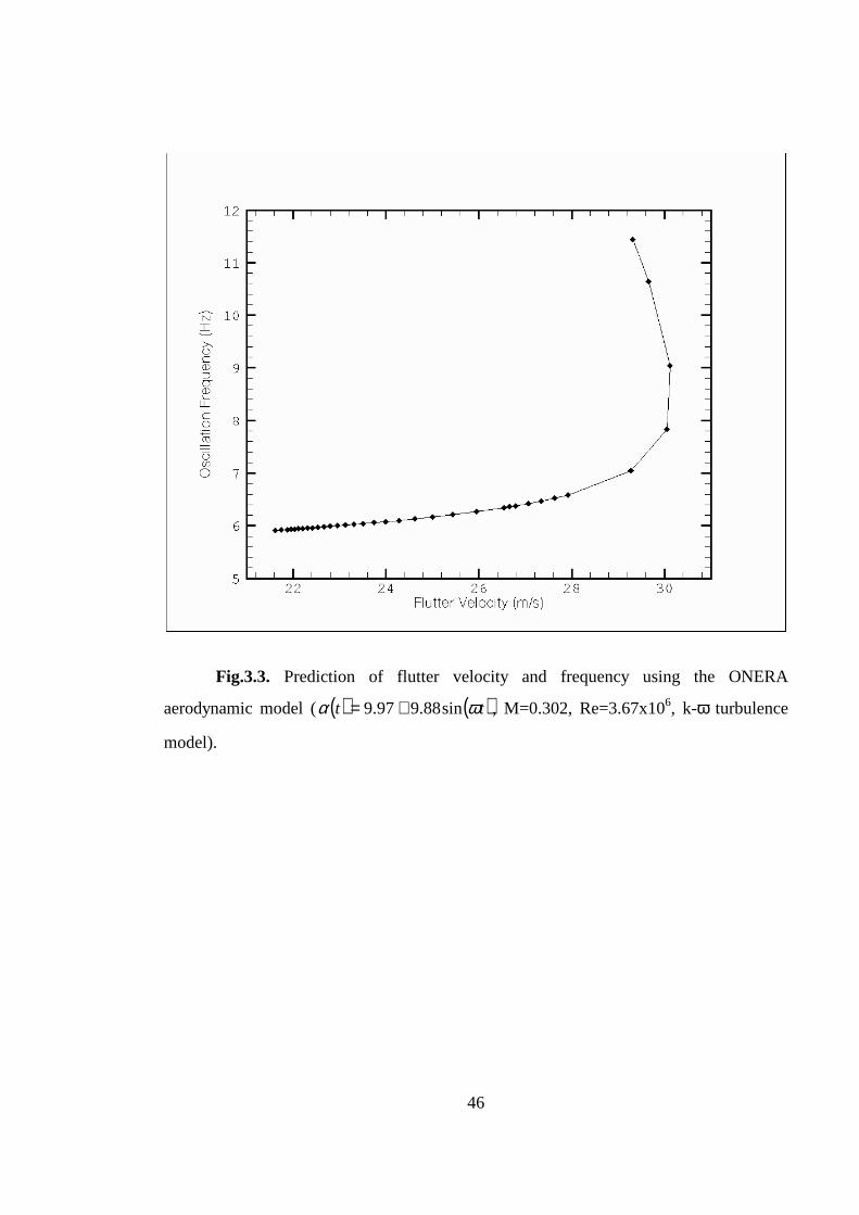
Once the fitting was done, the flutter program is run for all the cases using the

parameters r10, r12, r20, r22, r30 and r32 estimated before. Other constants and parameters

used in the flutter calculations are described in Table 3.4. The oscillation frequency

versus the flutter frequency has been plotted in Fig. 3.3. This shows the rapid increase in

the oscillations at the onset of flutter as is expected.

28

Chapter 4. Conclusions and suggestions for future work

4.1. Conclusions

A simple analytical method to include non-linear aerodynamic effects (by means

of the ONERA model) into a stall flutter analysis was developed. The analysis applies the

mathematical tools of Fourier analysis, harmonic balance and the Newton-Raphson as a

numerical solver. The PMB fluid dynamics solver was used to calculate the airloads (lift)

over an oscillating aerofoil using the k-ω turbulence model. The solutions compared well

with experimental results but further work must be carried to assess the impact of the

turbulence model used on the accuracy of the computational results. A numerical method

was used to fit the ONERA model to the fluid solver results. The fitting was satisfactory,

but due to the simplicity of the aeroelastic model the curves obtained were very simple,

just ellipses. The flutter calculations were qualitative satisfactory as well, predicting the

velocity and frequency of the onset of flutter.

4.2. Suggestions for future work

The computational grid used in this study was not very fine (150x50), and some

improvements over the present calculations would be done if working with a finer grid.

The time resolution used in the fluid solver was the minimum possible, and in future

works higher values might be used.

For stall cases, it might be good to fit the ONERA model for the moment

coefficient instead of doing it for the lift, as was done here. And, definitely, the quality of

the fitting would be improved by increasing the number of parameters.

There is scope to use this method of predicting aerodynamic loads within flight

dynamics codes as a replacement to look-up tables, which are currently used to give

aerofoil loadings. This model can be extended to predict three-dimensional aerodynamics

on finite wings and rotor-blades, and hence improve prediction methods for flutter

analysis.

29

To further validate the code in the form it is currently, a set of experimental data

should be obtained, including both aerodynamic loads and flutter characteristics, and a

comparison between the prediction and the experiments carried out.

30

References

1.1. Fung, Y.C., “An Introduction to the Theory of Aeroelasticity” , Dover

Publications, 1993.

1.2. Tran, C.T. and Petot, D., “Semi-Empirical Model for the Dynamic Stall of

Aerofoils in View of Application to the Calculation of Responses of a Helicopter in

Forward Flight” , Vertica, Vol.5, No.1, 1981, pp. 35-53.

1.3. Dat, D. and Tran, C.T., “ Investigation of the Stall Flutter of an Aerofoil with

a Semi-Empirical Model of 2-D Flow”, Vertica, Vol.7, No.2., 1983, pp. 73-86.

1.4. Marshall, J.G. and Imregun, M., “A Review of Aeroelasticity Methods with

Emphasis on Turbomachinery Applications” , Journal of Fluids and Structures, 10, 1996,

pp. 237-267.

1.5. Peters, D.A., “Toward a Unified Lift Model for Use in Rotor Blade Stability

Analyses” , Journal of the American Helicopter Society, Vol.30, No.3, 1985, pp. 32-42.

1.6. Petot, D. and Dat, R., “Unsteady Aerodynamic Loads on an Oscillating

Aerofoil with Unsteady Stall” , Proceedings of 2nd Workshop on Dynamics and

Aeroelasticity Stability Modelling of Rotorcraft Systems, Florida Atlantic Univ., Boca

Raton, FL, Nov. 1987.

1.7. Dunn, P. and Dugundji, J., “Nonlinear Stall Flutter and Divergence Analysis

of Cantilevered Graphite-Epoxy Wings” , AIAA Journal, Vol.30, No.1, 1992, pp. 153-162.

1.8. Chopra, I. and Dugundji, J., “Non-linear Dynamic Response of a Wind

Turbine Blade”, Journal of Sound and Vibration, Vol.63, No.2, 1979, pp. 265-286.

1.9. Tang, D. and Dowell, E., “Experimental and Theoretical Study for Non-linear

Aeroelastic Behaviour of Flexible Rotor Blades” , AIAA Paper 92-2253, April 1992.

1.10 Hodges, D. and Dowell, E., “Non-linear Equations of Motion for the Elastic

Bending and Torsion of Twisted Non-uniform Rotor Blades” , NASA TN D-7818, Dec.

1974.

1.11. Kim, T. and Dugundji, J., “Non-linear Large Amplitude Aeroelastic

Behaviour of Composite Rotor Blades” , AIAA Journal, Vol.31, No.8, 1993, pp. 1489-

1497.

31

1.12. Abdel-Rahim, A., Sisto, F. and Thangam, S., “Computational Study of Stall

Flutter in Linear Cascades” , ASME Journal of Turbomachinery, Vol. 115, 1993, pp. 157-

166.

1.13. Jang, H.M., Ekaterinaris, J.A., Platzer, M.F. and Cebeci, T., “Essential

Ingredients for the Computation of Steady and Unsteady Boundary Layers” , ASME

Journal of Turbomachinery, Vol.113, 1991, pp.608-616.

1.14. Cebeci, T., Platzer, M.F., Jang, H.M., and Chen, H.H., “An Inviscid-Viscous

Interaction Approach to the Calculation of Dynamic Stall Initiation on Aerofoils” , ASME

Journal of Turbomachinery, Vol.115, 1993, pp. 714-723.

1.15. Clarkson, J.D., Ekaterinaris, J.A., and Platzer, M.F., “Computational

Investigation of Aerofoil Stall Flutter” , Unsteady Aerodynamics, Aeroacoustics and

Aeroelasticity of Turbomachines and Propellers, H.M. Atassi, ed. Springer-Verlag, New

York, 1993, pp. 415-432.

1.16. McCroskey, W.J., “The Phenomenon of Dynamic Stall” , NASA TM-81264,

Mar. 1981.

1.17. Srinivasan, G.R., Ekaterinaris, J.A. and McCroskey, W.J., “Dynamic Stall of

an Oscillating Wing, Part 1: Evaluation of Turbulence Models” , AIAA Paper 93-3403,

August 1993.

1.18. Ekaterinaris, J.A. and Menter, F.R., “Computation of Separated and

Unsteady Flows with One and Two Equation Turbulence Models” , AIAA Paper 94-0190,

January 1994.

1.19. Ekaterinaris, J.A., Chandrasekhara, M.S. and Platzer, M.F., “Analysis of

Low Reynolds Number Aerofoils” , AIAA Paper 94-0534, January 1994.

1.20. Ekaterinaris, J.A. and Platzer, M.F., “Numerical Investigation of Stall

Flutter” , Journal of Turbomachinery, Vol. 118, April 1996, pp. 197-203.

1.21. Carta, F.O. and Lorber, P.F., “Experimental Study of the Aerodynamics of

Incipient Tortional Stall Flutter” , Journal of Propulsion, Vol.3., No.2, 1987, pp. 164-170.

1.22. McCroskey, W.J., McAlister, K.W, Carr, L.W. and Pucci, S.L., “An

Experimental Study of Dynamic Stall on Advanced Aerofoil Sections. Volume 1:

Summary of the Experiment” , NASA-TM-84245-VOL-1, 1982.

32

1.23. Carr, L.W., “Progress in Analysis and Prediction of Dynamic Stall” , J.

Aircraft, 25 (1), Jan. 1988 pp. 6-17.

1.24. Visbal, M.R., “Effect of Compressibility on Dynamic Stall” , AIAA Paper

88-0132, 1988.

1.25. Piziali, R.A., “An Experimental Investigation of 2D and 3D Oscillating

Wing Aerodynamics for a range of angle of Attack including Stall” , NASA-TM-4632

(1993).

1.26. Ekaterinaris, J.A., Cricelli, A.S. and Platzer, M.F., “A Zonal Method for

Unsteady Viscous Compressible Aerofoil Flows”, Journal of Fluids and Structures, 8, pp.

107-123 (1994).

1.27. Mehta, U.B. and Lavan, Z., “Starting Vortex, Separation Bubbles and Stall:

A Numerical Study of Laminar Unsteady Flow Around an Aerofoil” , J. Fluid Mech.,

67(2), pp. 227-256 (1975).

1.28. Gulcat, U., “Separate Numerical Treatment of Attached and Detached Flow

Regions in General Viscous Flows”, Ph.D. Thesis, Georgia Institute of Technology,

Atlanta, Georgia, 1981.

1.29. Wu, J.C., “Zonal Solution of Unsteady Viscous Flow Problems”, AIAA

Paper 84-1637, 1984.

1.30. Wu, J.C., Wang, C.M. and Tuncer, I.H., “Unsteady Aerodynamics of

Rapidly Pitched Aerofoil” , AIAA Paper 86-1105, 1986.

1.31. Tuncer, I.H., “Unsteady Aerodynamics of Oscillating and Rapidly Pitched

Aerofoils” , Ph.D. Thesis, Georgia Institute of Technology, Atlanta, Georgia, 1988.

2.1. Tran, C.T. and Petot, D., “Semi-Empirical Model for the Dynamic Stall of

Aerofoils in View of Application to the Calculation of Responses of a Helicopter in

Forward Flight,” Vertica, Vol.5, No.1, 1981, pp. 35-53.

2.2. Meirovitch, L., “Elements of vibration analysis” , Mc-Graw Hill International

Editions, 2nd edition, 1986.

3.1. McAllister, K.W., Pucci, S.L., McCroskey, W.J. and Car, L.W., “An

Experimental Study of Dynamic Stall on Advanced Aerofoil Sections, vol. 2: Pressure

and Force Data” , NASA TM-84245, September 1982.

33

3.2. Press, W.H., Teukolsky, S.A., Vetterling, W.T. and Flannery, B.P.,

“Numerical recipes in FORTRAN. The art of scientific computing” , 2nd edition,

Cambridge University Press, 1992.

3.3. Marquardt, D.W., Journal of the Society for Industrial and Applied

Mathematics, vol.11, pp. 431-441, 1963.

34

Appendix 1

The symmetric part of the aerodynamic curves

If due to the oscillation amplitude negative values are reached, the symmetric

portion of the aerodynamic curve has to be considered.

Using α α1 1= − , the above three equations are expanded:

∆Cb

b

zv

v

v

v

01 1 0

1 1

1 1 01 1

2

2

= ⋅ ⋅ −�

��

�

�� ⋅ −���

��� +

�

�

� −

− ⋅ ⋅ −�

��

�

�� ⋅ +���

��� +

�

�

�

απ

α αα

φ π φ

απ

α αα

φ π φ

cos

cos

(A1.1)

∆Cb

b

zsv

v

11

1 1

11 1

2

1

22

2

1

22

= ⋅ ⋅ − −���

��� − ⋅�

�

� −

− ⋅ ⋅ − +���

��� − ⋅�

�

�

απ

φ π φ

απ

φ π φ

sin

sin

(A1.2)

∆Cb

b

zcv

v

21

1 1

11 1

1

2

1

63

1

2

1

63

= ⋅ ⋅ − ⋅ − ⋅�

�

� −

− ⋅ ⋅ − ⋅ − ⋅�

�

�

απ

φ φ

απ

φ φ

cos sin

cos sin

(A1.3)

Again:

φ δ11= −sin , -1<δ <1

φ π1 2

= , δ >1

φ π1 2

= − , δ <-1 (A1.4)

where δ α αα

= −1 0

v

35

Appendix 2

The Newton-Raphson method

The system of six equations (2.130-2.135) is solved by means of the Newton-

Raphson method.

First of all, the equations are written in the form:

Fi(x1,...x6)=0

The vector (x1,...x6) is called state vector. Here, it should include the harmonic

components of the modal amplitudes qi0, qis and qic. But, due to the possibility that the

iterative solution procedure converges to a trivial solution (zero), a different approach is

taken.

q2s (sine component of second mode) is set to a small constant which gives the

amplitude level of the oscillation, and q2c (cosine component) is set to zero since for limit

cycle oscillations we may consider any initial phase. The second mode (torsion) was

chosen since this mode dominates the oscillation behaviour.

To complete the vector of the unknowns, the missing components are replaced by

ka (reduced torsional frequency) and k (reduced frequency).

The Newton-Raphson method is used:

F x x F xFx

x H O Ti ii

jj

j

( ) ( ) . . .+ = + ⋅ + ==�δ ∂

∂δ 0

1

6

The summation is the Jacobian matrix. It is calculated numerically, increasing the

state vector by a small number. Then JF

x

F

xj j

= =∂∂

∆∆

.

Then, the correction is: δx J F x= − ⋅−1 ( ) , at the nth iteration. And the estimation of

the vector at the next iteration is: x x xn n+ = +1 δ .

For the present work 25 iterations are performed and if the change in variables is

less than 10-4 the iteration procedure is considered as divergent.

36

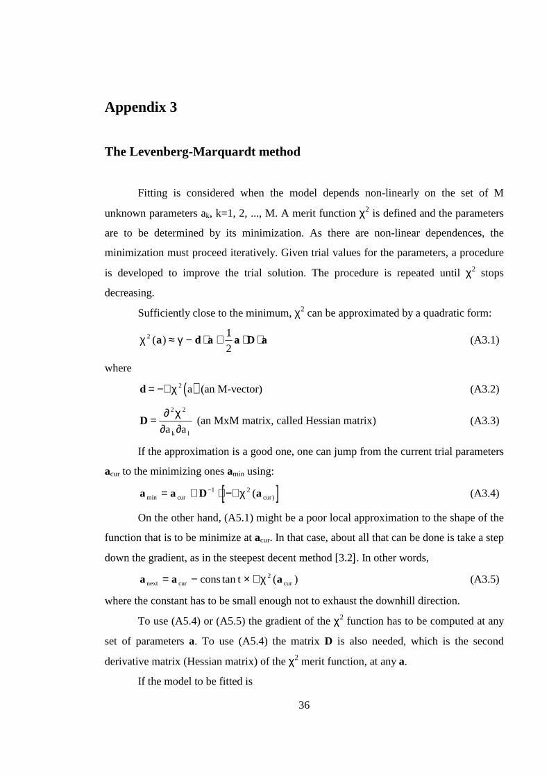
Appendix 3

The Levenberg-Marquardt method

Fitting is considered when the model depends non-linearly on the set of M

unknown parameters ak, k=1, 2, ..., M. A merit function χ2 is defined and the parameters

are to be determined by its minimization. As there are non-linear dependences, the

minimization must proceed iteratively. Given trial values for the parameters, a procedure

is developed to improve the trial solution. The procedure is repeated until χ2 stops

decreasing.

Sufficiently close to the minimum, χ2 can be approximated by a quadratic form:

χ γ2 1

2( )a d a a D a≈ − ⋅ + ⋅ ⋅ (A3.1)

where

( )d = −∇χ 2 a (an M-vector) (A3.2)

D =∂ χ

∂ ∂

2 2

a ak l

(an MxM matrix, called Hessian matrix) (A3.3)

If the approximation is a good one, one can jump from the current trial parameters

acur to the minimizing ones amin using:

[ ]a a D amin )(= + ⋅ −∇χ−cur cur

1 2 (A3.4)

On the other hand, (A5.1) might be a poor local approximation to the shape of the

function that is to be minimize at acur. In that case, about all that can be done is take a step

down the gradient, as in the steepest decent method [3.2]. In other words,

a a anext cur curcons t= − × ∇χtan ( )2 (A3.5)

where the constant has to be small enough not to exhaust the downhill direction.

To use (A5.4) or (A5.5) the gradient of the χ2 function has to be computed at any

set of parameters a. To use (A5.4) the matrix D is also needed, which is the second

derivative matrix (Hessian matrix) of the χ2 merit function, at any a.

If the model to be fitted is

37

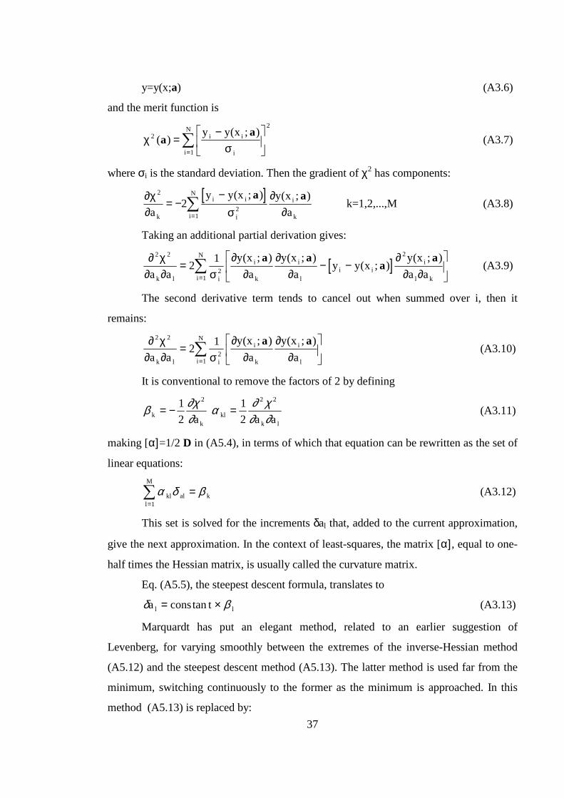
y=y(x;a) (A3.6)

and the merit function is

χσ

2

1

2

( )( ; )

aa

=−�

�

�

=�

y y xi i

ii

N

(A3.7)

where σi is the standard deviation. Then the gradient of χ2 has components:

[ ]∂χ

∂ σ∂

∂

2

21

2a

y y x y x

ak

i i

ii

Ni

k

= −−

=�

( ; ) ( ; )a a k=1,2,...,M (A3.8)

Taking an additional partial derivation gives:

[ ]∂ χ∂ ∂ σ

∂∂

∂∂

∂∂ ∂

2 2

2

2

1

21

a a

y x

a

y x

ay y x

y x

a ak l i

i

k

i

li i

i

l ki

N

= − −�

�

�

=�

( ; ) ( ; )( ; )

( ; )a aa

a (A3.9)

The second derivative term tends to cancel out when summed over i, then it

remains:

∂ χ

∂ ∂ σ∂

∂∂

∂

2 2

21

21

a a

y x

a

y x

ak l i

i

k

i

li

N

=�

�

�

=�

( ; ) ( ; )a a (A3.10)

It is conventional to remove the factors of 2 by defining

β ∂χ∂k

ka= − 1

2

2

α ∂ χ∂ ∂kl

k la a= 1

2

2 2

(A3.11)

making [α]=1/2 D in (A5.4), in terms of which that equation can be rewritten as the set of

linear equations:

α δ βkl al kl

M

==�

1

(A3.12)

This set is solved for the increments δal that, added to the current approximation,

give the next approximation. In the context of least-squares, the matrix [α], equal to one-

half times the Hessian matrix, is usually called the curvature matrix.

Eq. (A5.5), the steepest descent formula, translates to

δ βa cons tl l= ×tan (A3.13)

Marquardt has put an elegant method, related to an earlier suggestion of

Levenberg, for varying smoothly between the extremes of the inverse-Hessian method

(A5.12) and the steepest descent method (A5.13). The latter method is used far from the

minimum, switching continuously to the former as the minimum is approached. In this

method (A5.13) is replaced by:

38

δλα

βalll

l= 1 or λα δ βl l l la = (A3.14)

Marquardt’s second insight is that (A5.14) and (A5.12) can be combined if a new

matrix α‘ is defined with the following characteristics:

′ = +α α λjj jj ( )1

′ =α αjk jk (j≠k) (A3.15)

and then (A5.14) and (A5.12) are replaced by:

′ ==� α δ βkl al kl

M

1

(A3.16)

When λ is very large, the matrix α‘ is forced into being diagonally dominant, so

(A5.16) goes over to be identical to (A5.14). On the other hand, as λ approaches zero,

(A5.16) goes over to (A5.12).

Given an initial value for the set of fitted parameters a, the Marquardt recipe is as

follows:

- Compute χ2 (a).

- Pick a modest value for λ, say λ=0.001.

- (* ) Solve the linear equations (A5.16) for δa and evaluate χ2(a+δa).

- If χ2(a+δa)≥χ2(a), increase λ by a factor of 10 (or any substantial factor) and go

back to (* ).

- If χ2(a+δa)< χ2(a), decrease λ by a factor of 10, update the trial solution

a ← a+δa, and go back to (* ).

Iterating to convergence is generally wasteful and unnecessary since the minimum

is at best only a statistical estimate of the parameters a.

39

Appendix 4

Linear Aerodynamic Coefficients

The values for the linear coefficients used in the ONERA Model are found from

incompressible aerodynamics. Starting from the incompressible lift equation given by:

[ ] ( ) �

�

���

���

� +++−+−+−= θθρπθθρπ������

abUhKbUCbaUhbL2

122 (A4.1)

where a is the distance between the elastic axis and the mid-chord position. For this case,

2

1=a and h and θ are evaluated at the ¼ chord position. Replacing the time derivatives

( )⋅

and ( )⋅⋅

with dimensionless time ( )τ

where :

��

���

�=b

Utτ (A4.2)

gives the following:

[ ] ( ) �

�

���

���

� −++−+−+−= θθρπθθρπ�

�

����

ab

hKCbUbabhUl

2

12 22 (A4.3)

From this equation and the definition of angle of attack given by bh�

−= θα and using

21−=a it is possible to derive the following:

( )γγ

ρρ LLL cCUCCcUL 22

2

1

2

11

+−= (A4.4)

where

θπθππγ

���

��

ab

hCC LL −+−=−

1 (A4.5)

and

( ) �

�

���

���

� −++−= θππθπγ

�

�

ab

hKCCL 2

1222 (A4.6)

Using equation (A4.5) and the definitions of angle of attack and elastic axis gives:

40

γ

θπαπ LL CC ++=

21

Which gives the linear coefficients π=1LS , 22π=LS , and 03 =LS .

Using Theodorsen’s Function

( )22

2

212

2

K

KKF

++

=λ

λλ and ( ) ( )

221

21 1

K

KKG

+−

=λ

λλ (A4.7)

and the definition of angle of attack given earlier in equation (A4.6) results in the

following:

( )( ) ( )( )θαπθαπγγ

��

�

��

+++=+ 255.0215.015.0 LL CC (A4.8)

From this, 15.01 +λ , 55.02 +λ , and πα 20 =L

. This procedure can be repeated for the

moment coefficients in a similar manner.

41

Figures

Fig. 1.1. Cantilever wing of uniform cross section.

Fig.1.2. Variation of the lift coefficient (CL) with the angle of attack.

Angle of attack

CL

α1

(stall angle)

U

c

l

42

Fig.1.3. Two degree of freedom representation for an aerofoil.

U

U

b) Plunging a) Pitching

θ

�

h

U �

h

43

Fig.2.1. Definition of the variables in pitching and plunging motion.

Fig.2.2. Single break-point approximation of the deviation −Cz.

Cz

Ι Ι0 Ι1

Ιv Ιv −Cz

44

Fig. 2.3. Example of the oscillation over stall angle.

Fig. 2.4. Change of axis from 1/4 chord to 1/2 chord.

L1/2 L1/4

M1/2

M1/4

b/2 c

α α α φ= +0 v sin α

α1

α0

ϕ 2π π

∆Cz

ϕ1 π/2 ϕ

45

Fig.3.1. Comparison of the fitted and computed lift coefficients

( )sin(5)( tt ωα = , M=0.302, Re=3.67x106, k-ω turbulence model).

Fig.3.2. Comparison of the fitted and computed lift coefficients

(α ω( ) . . sin( )t t= +9 97 988 , M=0.302, Re=3.67x106, k-ω turbulence model).

46

Fig.3.3. Prediction of flutter velocity and frequency using the ONERA

aerodynamic model ( ( ) ( )tt ωα sin88.997.9 += , M=0.302, Re=3.67x106, k-ω turbulence

model).

47

Tables

Table number

Description

Table 3.1. Description of the cases solved using the fluid solver.

Table 3.2. Parameters r10, r12, r20, r22, r30 and r32 obtained with the fitting.

Table 3.3. Harmonic decomposition of the computed and experimental lift

coefficient curves.

Table 3.4. Parameters and constants used in the flutter program.

48

Case Mean angle of

attack (deg.)

Amplitude of

vibration (deg.)

Reduced

frequency

Mach

number

Reynolds

number

1 0 5 0.145 0.302 3.67e6

2 9.97 9.88 0.145 0.302 3.67e6

Table 3.1. Description of the cases solved using the fluid solver.

Case r10 r12 r20 r22 r30 r32

1 -9.1813 -19.4247 1.2356 1.2416 -6078.1 19.3940

2 -5.6958 -17.4499 0.6425 1.6833 -0.8193 16.3939

Exper. Data -3.8187 -8.1573 0.5241 1.0171 -0.6695 17.1221

Table 3.2. Parameters r10, r12, r20, r22, r30 and r32 obtained with the fitting.

Case CL0 CLs1 CLc1 CLs2 CLc2

1 0.0872 0.0166 0.3183 -0.0226 -0.2177

2 0.7335 -0.1923 -0.1663 0.3535 0.2122

Exper. Data 0.7730 -0.1924 -0.1445 0.3563 0.1934

Table 3.3. Harmonic decomposition of the computed and experimental lift

coefficient curves.

49

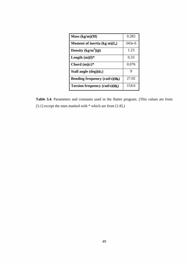
Mass (kg/m)(M) 0.283

Moment of inertia (kg m)(Ia) 343e-6

Density (kg/m3)(ρρρρ) 1.23

Length (m)(l)* 0.33

Chord (m)(c)* 0.076

Stall angle (deg)(αααα1) 9

Bending frequency (rad/s)(ωωωωh) 27.02

Torsion frequency (rad/s)(ωωωωa) 154.6

Table 3.4. Parameters and constants used in the flutter program. (This values are from

[3.1] except the ones marked with * which are from [1.8].)

50

Guide to computer programs

1. Introduction

Two different programs were used in the project, apart from the CFD code: the

fitting program and the flutter one. The fitting program is based on the ONERA model,

and tries to fit that model to a given lift coefficient loop in order to obtain the ri

coefficients of the non-linear equation of the ONERA model. It works following the

Levenberg-Marquardt method. The flutter program calculates, using the ONERA model

for the aerodynamic part, the flutter velocity and frequency for a given conditions on an

aerofoil.

2. Fitting program

The variables that the program needs are introduced in a file called ‘aeroel2.in’

and are summarised in the following table. Apart from those variables, the program also

needs a file with the values of the lift coefficient, which are to be fitted to. This file is

named ‘ lift.dat’ . It contains two columns: the first column is the angle of attack and the

second one the lift coefficient. These values can come from experiments or from a CFD

code.

The output of the program is written in the file ‘aeroel2.out’ . It contains the best-

fit values for the parameters r10, r20, r30, r12, r22 and r32 and the value of chi-square, which

measures the agreement between the input file and the calculated coefficient, followed by

the lift or moment coefficient calculated using those parameters for every angle of attack

of the input file (‘ lift.dat’ ).

The program was used in the following way: after obtaining a set of values for the

lift coefficient using the flow solver (it could be obtained by means of experiments), these

values are introduced in the ‘ lift.dat’ file. The characteristics of the case are introduced in

the ‘aeroel2.in’ file. The parameter NFIT is set to 1, in order to carry out the fitting, and

then the program is run. The ri parameters and the calculated lift coefficient are available

in the ‘aeroel2.out’ file. Once the parameters are estimated for the lift coefficient, the

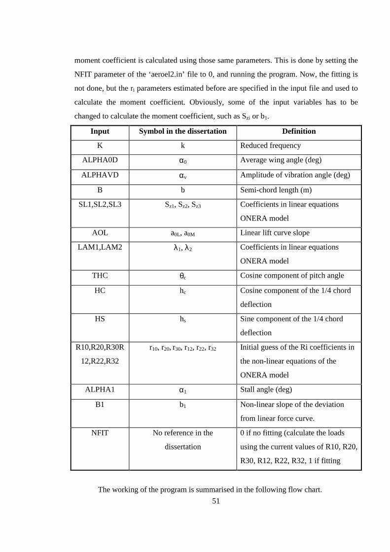
51

moment coefficient is calculated using those same parameters. This is done by setting the

NFIT parameter of the ‘aeroel2.in’ file to 0, and running the program. Now, the fitting is

not done, but the ri parameters estimated before are specified in the input file and used to

calculate the moment coefficient. Obviously, some of the input variables has to be

changed to calculate the moment coefficient, such as Szi or b1.

Input Symbol in the dissertation Definition

K k Reduced frequency

ALPHA0D α0 Average wing angle (deg)

ALPHAVD αv Amplitude of vibration angle (deg)

B b Semi-chord length (m)

SL1,SL2,SL3 Sz1, Sz2, Sz3 Coefficients in linear equations

ONERA model

AOL a0L, a0M Linear lift curve slope

LAM1,LAM2 λ1, λ2 Coefficients in linear equations

ONERA model

THC θc Cosine component of pitch angle

HC hc Cosine component of the 1/4 chord

deflection

HS hs Sine component of the 1/4 chord

deflection

R10,R20,R30R

12,R22,R32

r10, r20, r30, r12, r22, r32 Initial guess of the Ri coefficients in

the non-linear equations of the

ONERA model

ALPHA1 α1 Stall angle (deg)

B1 b1 Non-linear slope of the deviation

from linear force curve.

NFIT No reference in the

dissertation

0 if no fitting (calculate the loads

using the current values of R10, R20,

R30, R12, R22, R32, 1 if fitting

The working of the program is summarised in the following flow chart.

52

Start

Input

Fitting No

Yes

λ<0

Calculate chisq(a)

Calculate δa

Calculate chisq(a+δa)

chisq(a)> chisq(a+δa)

No

No

Yes Yes

λ=0.1λ a=a+δa

λ=10λ No. iterat. = 25

No. iterat. = 25

Yes

No λ=0

Calculate covariance

Calculate loads for current a

End

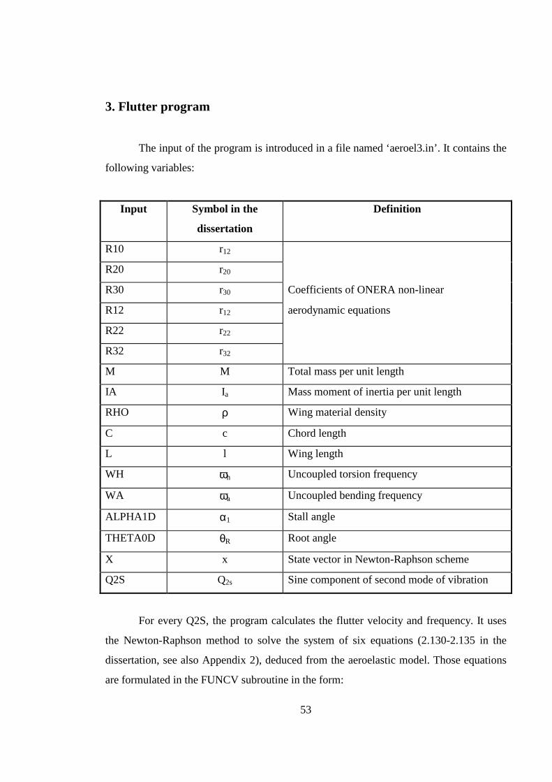
53

3. Flutter program

The input of the program is introduced in a file named ‘aeroel3.in’ . It contains the

following variables:

Input Symbol in the

dissertation

Definition

R10 r12

R20 r20

R30 r30 Coefficients of ONERA non-linear

R12 r12 aerodynamic equations

R22 r22

R32 r32

M M Total mass per unit length

IA Ia Mass moment of inertia per unit length

RHO ρ Wing material density

C c Chord length

L l Wing length

WH ωh Uncoupled torsion frequency

WA ωa Uncoupled bending frequency

ALPHA1D α1 Stall angle

THETA0D θR Root angle

X x State vector in Newton-Raphson scheme

Q2S Q2s Sine component of second mode of vibration

For every Q2S, the program calculates the flutter velocity and frequency. It uses

the Newton-Raphson method to solve the system of six equations (2.130-2.135 in the

dissertation, see also Appendix 2), deduced from the aeroelastic model. Those equations

are formulated in the FUNCV subroutine in the form:

54

Fi(x1,...x6)=0 (FVEC or P in the program)

The vector (x1,...x6) is called state vector. It includes q10 (mean component of first

mode, bending), q20 (mean component of second mode, torsion), q1s (sine component of

first mode), q1c (cosine component of first mode), ka (reduced torsional frequency, k2 in

the program) and k (reduced frequency).

The Newton-Raphson method is used:

F x x F xF

xx H O Ti i

i

jj

j

( ) ( ) . . .+ = + ⋅ + ==�δ

∂∂

δ 01

6

The summation is the Jacobian matrix. It is calculated numerically in the FDJAC

subroutine, increasing the state vector by a small number. Then JFx

Fxj j

= =∂∂

∆∆

.

Thus, the correction is: δx J F(x= − ⋅−1 ) , at the nth iteration. The inverse of the

Jacobian matrix is calculated using the subroutines LUDCMP and LUBKSB. And the

estimation of the vector at the next iteration is: x x xn n+ = +1 δ .

For the present work 25 iterations are performed and if the change in variables is

not less than 10-4 the iteration procedure is considered as divergent.

The output of the program is written to a file called ‘aeroel3.out’ . It contains, in

columns, Q2S (which was an input), the x vector (which is actually q10, q20, q1s, q1c, k2

and k), the flutter velocity (FS in the program), the flutter frequency (FQ), the mean angle

of attack (ALPHA0D), and the amplitude of vibration (AVIBD).

The program is summarised in the following flow chart.

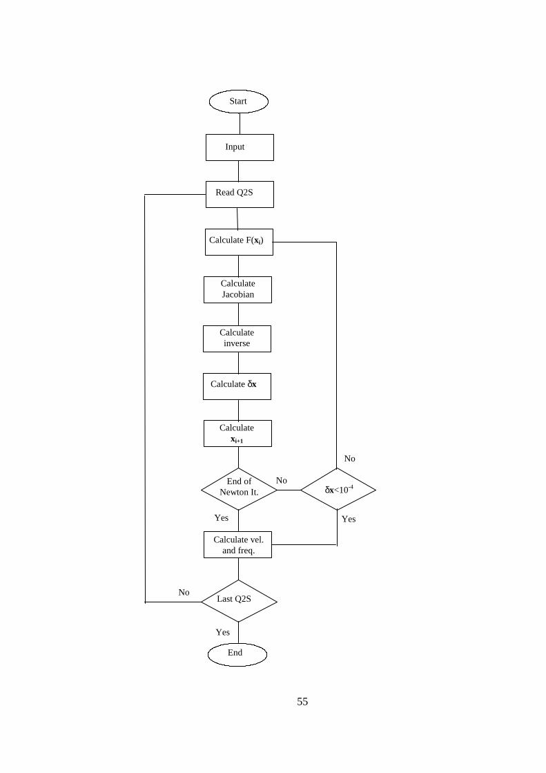
55

Start

Input

Read Q2S

Calculate F(xi)

Calculate Jacobian

Calculate inverse

Calculate δx

No

Yes

Calculate vel. and freq.

Calculate xi+1

End of Newton It. δx<10-4

Yes

No

Last Q2S

End

Yes

No

56

4. Listings

4.1. Fitting program

PROGRAM FI T CCCCCCCCCCCCCCCCCCCCCCCCCCCCCCCCCCCCCCCCCCCCCCCCCCCCCCCCCCCCCCCCCCCCCCC C FI TTI NG PROGRAM TO ESTI MATE THE Ri PARAMETERS OF THE C NON- LI NEAR EQUATI ON OF THE ONERA MODEL C C I NPUT: ' l i f t . dat ' : CONTAI NS THE LI FT COEFFI CI ENT LOOP TO FI T TO C C K REDUCED FREQUENCY C ALPHA0D AVERAGE WI NG ANGLE ( DEG) C ALPHAVD VI BRATI ON ANGLE ( DEG) C B SEMI CHORD LENGTH ( M) C SL1, SL2, SL3 COEFFI CI ENTS I N LI NEAR EQUATI ONS ONERA MODEL C AOL LI NEAR LI FT CURVE SLOPE C LAM1, LAM2 COEFFI CI ENTS I N LI NEAR EQUATI ONS ONERA MODEL C THC COSI NE COMPONENT OF THE PI TCH ANGLE C HC COSI NE COMPONENT OF THE 1/ 4 CHORD DEFLECTI ON C HS SI NE COMPONENT OF THE 1/ 4 CHORD DEFLECTI ON C R10, R20, R30, I NI TI AL GUESS OF THE Ri COEFFI CI ENTS C R12, R22, R32 I N THE NON- LI NEAR EQUATI ONS OF THE ONERA MODEL C ALPHA1 STALL ANGLE ( DEG) C B1 NON- LI NEAR SLOPE OF THE DEVI ATI ON FROM LI NEAR FORCE CURVE C NFI T 0 FOR NO FI TTI NG ( CALCULATES THE LOADS USI NG THE CURRENT C VALUES OF R10, R20, R30, R12, R22, R32, 1 I F FI TTI NG I S REQUI RED C CCCCCCCCCCCCCCCCCCCCCCCCCCCCCCCCCCCCCCCCCCCCCCCCCCCCCCCCCCCCCCCCCCCCCCC C DI MENSI ON EXPERZ( 500) , EXPERA( 500) , SI G( 500) DI MENSI ON APAR( 6) , LI STA( 6) , COVAR( 500, 500) , ALPHA( 500, 500) EXTERNAL FLI FT C REAL B, SL1, SL2, SL3, AOL, LAM1, LAM2, THC, HC, HS, ALPHA1, B1, K, F ALPHA0D, ALPHAVD, R10, R20, R30, R12, R22, R32, Z COMMON/ L/ B, SL1, SL2, SL3, AOL, LAM1, LAM2, THC, HC, HS COMMON/ NL/ ALPHA1, B1 COMMON/ FUN/ K, ALPHA0D, ALPHAVD NA=6 C C READ THE FI LE CONTAI NI NG THE VALUES TO FI T TO C NEXPER NUMBER OF POI NTS TO FI T C EXPERA( I ) ANGLE OF ATTACK ( DEG) C EXPERZ( I ) LI FT COEFFI CI ENT C I =1 OPEN ( 11, FI LE=' l i f t . dat ' , STATUS=' OLD' ) CG222 READ ( 11, * , END=333) a1, a2, a3, EXPERA( I ) , EXPERZ( I ) 222 READ ( 11, * , END=333) EXPERA( I ) , EXPERZ( I ) I =I +1 GOTO 222 333 CLOSE( 11) NEXPER=I - 1 C C READ THE VARI ABLES TO BE USED I N THE PROGRAM C OPEN( 10, FI LE=' aer oel 2. i n' , STATUS=' OLD' ) READ ( 10, 7000) K, ALPHA0D, ALPHAVD, B, SL1, SL2, SL3, AOL READ ( 10, 7000) LAM1, LAM2, THC, HC, HS, R10, R12, R20 READ ( 10, 7000) R22, R30, R32, ALPHA1, B1 READ ( 10, 7000) LI STA( 1) , LI STA( 2) , LI STA( 3) , F LI STA( 4) , LI STA( 5) , LI STA( 6) READ ( 10, * ) NFI T READ ( 10, * ) NI TS C C I NI TI AL GUESSES FOR THE Ri PARAMETERS ARE PUT I NTO APAR. C APAR( 1) =R10

57

APAR( 2) =R20 APAR( 3) =R30 APAR( 4) =R12 APAR( 5) =R22 APAR( 6) =R32 C C CREATES THE OUTPUT FI LE C OPEN( 9, FI LE=' aer oel 2. out ' , STATUS=' UNKNOWN' ) C C I F NFI T. EQ. 0 FI TTI NG I S NOT DONE, GOES DI RECTLY TO THE CALCULATI ON C USI NG THE CURRENT Ri . ELSE, THE FI TTI NG I S DONE. C I F ( NFI T. EQ. 0) GOTO 2 C C FI TTI NG BEGI NS. C NCA=500 DO I =1, NEXPER SI G( I ) =1. ENDDO ALPHA1=ALPHA1* 3. 141593/ 180. 0 C C I NI TI AL CALL TO MRQMI N. ALAMBDA I S RETURNED ON THE FI RST AND ALL C SUBSEQUENT CALLS AS THE SUGGESTED VALUE OF LAMBDA FOR THE NEXT C I TERATI ON; A I S ALWAYS RETURNED AS THE BEST PARAMETERS FOUND SO FAR. C ALAMDA=- 1 CALL MRQMI N( EXPERA, EXPERZ, SI G, NEXPER, APAR, LI STA, 6, F COVAR, ALPHA, NCA, CHI SQ, FLI FT, ALAMDA) C C CALL MRQMI N NI TS TI MES, ENOUGH TO ACHI EVE GOOD RESULTS. C NCON=0 111 CONTI NUE CALL MRQMI N( EXPERA, EXPERZ, SI G, NEXPER, APAR, LI STA, 6, F COVAR, ALPHA, NCA, CHI SQ, FLI FT, ALAMDA) NCON=NCON+1 I F ( NCON. LT. NI TS) GOTO 111 C C ALAMDA I S SET TO ZERO BEFORE THE FI NAL CALL TO MRQMI N C ALAMDA=0. 0 CALL MRQMI N( EXPERA, EXPERZ, SI G, NEXPER, APAR, LI STA, 6, F COVAR, ALPHA, NCA, CHI SQ, FLI FT, ALAMDA) C C OUTPUT WRI TTEN I N THE OUTPUT FI LE. APAR( i ) CORRESPONDS TO Ri C WRI TE( 9, 8000) APAR( 1) , APAR( 2) , APAR( 3) , APAR( 4) , APAR( 5) , APAR( 6) WRI TE( 9, 8001) CHI SQ C C USI NG THE ESTI MATED Ri , THE LI FT OR MOMENT COEFFI CI ENT I S C CALCULATED AND WRI TTEN TO ' aer oel 2. out ' , FOR EVERY ANGLE C OF ATTACK OF THE ' l i f t . dat ' FI LE. C 2 DO L=1, NEXPER NF=1 I F ( L. EQ. 1) THEN CGSOS CALL FLI FT( EXPERA( L) , - 13. , APAR, NF, Z, DYDA, NA) CALL FLI FT( EXPERA( L) , EXPERA( NEXPER) , APAR, NF, Z, DYDA, NA) ELSE CALL FLI FT( EXPERA( L) , EXPERA( L- 1) , APAR, NF, Z, DYDA, NA) ENDI F ENDDO STOP C C FORMAT STATEMENTS C 7000 FORMAT( 1X, F10. 5) 8000 FORMAT( 1X, ' #' , 6( 1X, F10. 4) ) 8001 FORMAT( 1X, ' #' , ( 1X, F10. 4) ) END CCCCCCCCCCCCCCCCCCCCCCCCCCCCCCCCCCCCCCCCCCCCCCCCCCCCCCCCCCCC SUBROUTI NE FUNCVL( ALPHA0, AVI B, K, PHI , THETA, CLGO, PLS, PLC, F, G, P) C CALCULATE LI NEAR LI FT. P I S CL1 I N THE TEXT OF THE DI SSERTATI ON C PLS AND PLC ARE THE SI N AND COS COMPONENTS OF THE LI NEAR C CONTRI BUTI ON TO THE GENERAL AERODYNAMI C FORCE COEFFI CI ENT. REST C OF THE VARI ABLES FOLLOW THE NOMENCLATURE OF THE DI SSERTATI ON.

58

CCCCCCCCCCCCCCCCCCCCCCCCCCCCCCCCCCCCCCCCCCCCCCCCCCCCCCCCCCCC REAL SL1, SL2, SL3, AOL, LAM1, LAM2, ALPHA0, AVI B, F THC, P, PHI , K, HC, HS, B, THETA, PLS, PLC, LS, LC, F, G, CLGO, CLGS, CLGC COMMON/ L/ B, SL1, SL2, SL3, AOL, LAM1, LAM2, THC, HC, HS C LS=AOL* ( AVI B- K* HC/ B- K* THC) LC=AOL* ( THC+K* HS/ B+K* AVI B) F=( K* K* LAM2+LAM1* LAM1) / ( LAM1* LAM1+K* K) G=K* LAM1* ( LAM2- 1) / ( LAM1* LAM1+K* K) CLGO=AOL* ALPHA0 CLGS=F* LS- G* LC CLGC=G* LS+F* LC THETA=ALPHA0+AVI B* SI N( PHI ) +THC* COS( PHI ) PLS=SL1* ( - K* THC- ( HS/ B) * K* K) - SL2* AVI B* K* K- SL3* K* THC +CLGS PLC=SL1* ( AVI B* K- ( HC/ B) * K* K) - SL2* THC* K* K+SL3* K* AVI B+CLGC P=CLGO+PLS* SI N( PHI ) +PLC* COS( PHI ) C RETURN END CCCCCCCCCCCCCCCCCCCCCCCCCCCCCCCCCCCCCCCCCCCCCCCCCCCCCCCCCCCC SUBROUTI NE FUNCVN( A, NA, ALPHA0, AVI B, R1, R2, R3, K, PHI , CZ2C2, CZ2S2, F CZ2C1, CZ2S1, CZ20, P2, F D_P2_DR10, D_P2_DR20, D_P2_DR30, D_P2_DR12, D_P2_DR22, D_P2_DR32) C CALCULATE NON- LI NEAR PART OF THE LI FT. P2 I S THE NON- LI NEAR C CONTRI BUTI ON TO THE GENERAL AERODYNAMI C LI FT COEFFI CI ENT. C DERI VATI VES OF P2 WI TH RESPECT TO THE PARAMETERS Ri ARE C CALCULATED. THEY ARE NECESSARY TO DO THE FI TTI NG. CCCCCCCCCCCCCCCCCCCCCCCCCCCCCCCCCCCCCCCCCCCCCCCCCCCCCCCCCCCC REAL A( NA) , DCZ0, DCZS1, DCZC2, R0, RS1, RC1, RS2, K1, K2, K3, K4, CZ2C2, F CZ2S2, CZ2C1, CZ2S1, CZ20, ALPHA1, B1, ALPHA0, AVI B, R1, R2, R3, F PHI 1, K, P2, PHI , PENT2, PHI 1T, R10, R20, R30, R12, R22, R32, ALPHA1T COMMON/ NL/ ALPHA1, B1 C R10=A( 1) R20=A( 2) R30=A( 3) R12=A( 4) R22=A( 5) R32=A( 6) ALPHA1T=- ALPHA1 PENT=( ALPHA1- ALPHA0) / AVI B I F ( PENT. GT. 1. ) THEN PHI 1=1. 571 ELSE I F ( PENT. LT. - 1. ) THEN PHI 1=- 1. 571 ELSE PHI 1=ASI N( PENT) ENDI F PENT2=( ALPHA1T- ALPHA0) / AVI B I F ( PENT2. GT. 1. ) THEN PHI 1T=1. 571 ELSE I F ( PENT2. LT. - 1. ) THEN PHI 1T=- 1. 571 ELSE PHI 1T=ASI N( PENT2) ENDI F C DCZ0 =( B1* AVI B/ 3. 14159) * ( - PENT* ( 1. 571- PHI 1 ) +COS( PHI 1 ) ) F - ( B1* AVI B/ 3. 14159) * ( PENT2* ( 1. 571+PHI 1T) +COS( PHI 1T) ) DCZS1=( B1* AVI B/ 3. 14159) * ( ( 1. 571- PHI 1 ) - 0. 5* SI N( 2. * PHI 1 ) ) F - ( B1* AVI B/ 3. 14159) * ( - ( 1. 571+PHI 1T) - 0. 5* SI N( 2. * PHI 1T) ) DCZC2=( B1* AVI B/ 3. 14159) * ( - . 5* COS( PHI 1 ) - 0. 166667* COS( 3. * PHI 1 ) ) F - ( B1* AVI B/ 3. 14159) * ( - . 5* COS( PHI 1T) - 0. 166667* COS( 3. * PHI 1T) ) R1=R10+R12* DCZ0* DCZ0 R2=( R20+R22* DCZ0* DCZ0) * * 2 R3=( R30+R32* DCZ0* DCZ0) * R20 K1=R2- K* K K2=R1* K K3=R2- 4* K* K K4=2* R1* K R0=- R2* DCZ0 RS1=- R2* DCZS1 RC1=- R3* K* DCZS1 RS2=2* R3* K* DCZC2 RC2=- R2* DCZC2 CZ20=R0/ R2 CZ2S1=( K1* RS1+K2* RC1) / ( K1* K1+K2* K2) CZ2C1=( K1* RC1- K2* RS1) / ( K1* K1+K2* K2)

59

CZ2S2=( K3* RS2+K4* RC2) / ( K3* K3+K4* K4) CZ2C2=( K3* RC2- K4* RS2) / ( K3* K3+K4* K4) P2=CZ20+CZ2S1* SI N( PHI ) +CZ2C1* COS( PHI ) F +CZ2S2* SI N( 2. * PHI ) +CZ2C2* COS( 2. * PHI ) C C DERI VATI VES C D_R1_DR10=1. D_R1_DR20=0. D_R1_DR30=0. D_R1_DR12=DCZ0* DCZ0 D_R1_DR22=0. D_R1_DR32=0. C D_R2_DR10=0. D_R2_DR20=2. * ( R20+R22* DCZ0* DCZ0) D_R2_DR30=0. D_R2_DR12=0. D_R2_DR22=2. * ( R20+R22* DCZ0* DCZ0) * DCZ0* DCZ0 D_R2_DR32=0. C D_R3_DR10=0. D_R3_DR20=R30+R32* DCZ0* DCZ0 D_R3_DR30=R20 D_R3_DR12=0. D_R3_DR22=0. D_R3_DR32=DCZ0* DCZ0* R20 C D_R0_DR10=- DCZ0* D_R2_DR10 D_R0_DR20=- DCZ0* D_R2_DR20 D_R0_DR30=- DCZ0* D_R2_DR30 D_R0_DR12=- DCZ0* D_R2_DR12 D_R0_DR22=- DCZ0* D_R2_DR22 D_R0_DR32=- DCZ0* D_R2_DR32 C D_RS2_DR10=2. * K* DCZC2* D_R3_DR10 D_RS2_DR20=2. * K* DCZC2* D_R3_DR20 D_RS2_DR30=2. * K* DCZC2* D_R3_DR30 D_RS2_DR12=2. * K* DCZC2* D_R3_DR12 D_RS2_DR22=2. * K* DCZC2* D_R3_DR22 D_RS2_DR32=2. * K* DCZC2* D_R3_DR32 C D_RC2_DR10=- DCZC2* D_R2_DR10 D_RC2_DR20=- DCZC2* D_R2_DR20 D_RC2_DR30=- DCZC2* D_R2_DR30 D_RC2_DR12=- DCZC2* D_R2_DR12 D_RC2_DR22=- DCZC2* D_R2_DR22 D_RC2_DR32=- DCZC2* D_R2_DR32 C D_RC1_DR10=- K* DCZS1* D_R3_DR10 D_RC1_DR20=- K* DCZS1* D_R3_DR20 D_RC1_DR30=- K* DCZS1* D_R3_DR30 D_RC1_DR12=- K* DCZS1* D_R3_DR12 D_RC1_DR22=- K* DCZS1* D_R3_DR22 D_RC1_DR32=- K* DCZS1* D_R3_DR32 C D_RS1_DR10=- DCZS1* D_R2_DR10 D_RS1_DR20=- DCZS1* D_R2_DR20 D_RS1_DR30=- DCZS1* D_R2_DR30 D_RS1_DR12=- DCZS1* D_R2_DR12 D_RS1_DR22=- DCZS1* D_R2_DR22 D_RS1_DR32=- DCZS1* D_R2_DR32 C D_K1_DR10=D_R2_DR10 D_K1_DR20=D_R2_DR20 D_K1_DR30=D_R2_DR30 D_K1_DR12=D_R2_DR12 D_K1_DR22=D_R2_DR22 D_K1_DR32=D_R2_DR32 C D_K2_DR10=K* D_R1_DR10 D_K2_DR20=K* D_R1_DR20 D_K2_DR30=K* D_R1_DR30 D_K2_DR12=K* D_R1_DR12 D_K2_DR22=K* D_R1_DR22 D_K2_DR32=K* D_R1_DR32 C D_K3_DR10=D_R2_DR10

60

D_K3_DR20=D_R2_DR20 D_K3_DR30=D_R2_DR30 D_K3_DR12=D_R2_DR12 D_K3_DR22=D_R2_DR22 D_K3_DR32=D_R2_DR32 C D_K4_DR10=2* K* D_R1_DR10 D_K4_DR20=2* K* D_R1_DR20 D_K4_DR30=2* K* D_R1_DR30 D_K4_DR12=2* K* D_R1_DR12 D_K4_DR22=2* K* D_R1_DR22 D_K4_DR32=2* K* D_R1_DR32 C D_CZ2S1_DR10=( D_K1_DR10* RS1+K1* D_RS1_DR10+D_K2_DR10* RC1+ F K2* D_RC1_DR10) / ( K1* K1+K2* K2) - F ( K1* RS1+K2* RC1) * ( 2. * K1* D_K1_DR10+2. * K2* D_K2_DR10) F / ( K1* K1+K2* K2) D_CZ2S1_DR20=( D_K1_DR20* RS1+K1* D_RS1_DR20+D_K2_DR20* RC1+ F K2* D_RC1_DR20) / ( K1* K1+K2* K2) - F ( K1* RS1+K2* RC1) * ( 2. * K1* D_K1_DR20+2. * K2* D_K2_DR20) F / ( K1* K1+K2* K2) D_CZ2S1_DR30=( D_K1_DR30* RS1+K1* D_RS1_DR30+D_K2_DR30* RC1+ F K2* D_RC1_DR30) / ( K1* K1+K2* K2) - F ( K1* RS1+K2* RC1) * ( 2. * K1* D_K1_DR30+2. * K2* D_K2_DR30) F / ( K1* K1+K2* K2) D_CZ2S1_DR12=( D_K1_DR12* RS1+K1* D_RS1_DR12+D_K2_DR12* RC1+ F K2* D_RC1_DR12) / ( K1* K1+K2* K2) - F ( K1* RS1+K2* RC1) * ( 2. * K1* D_K1_DR12+2. * K2* D_K2_DR12) F / ( K1* K1+K2* K2) D_CZ2S1_DR22=( D_K1_DR22* RS1+K1* D_RS1_DR22+D_K2_DR22* RC1+ F K2* D_RC1_DR22) / ( K1* K1+K2* K2) - F ( K1* RS1+K2* RC1) * ( 2. * K1* D_K1_DR22+2. * K2* D_K2_DR22) F / ( K1* K1+K2* K2) D_CZ2S1_DR32=( D_K1_DR32* RS1+K1* D_RS1_DR32+D_K2_DR32* RC1+ F K2* D_RC1_DR32) / ( K1* K1+K2* K2) - F ( K1* RS1+K2* RC1) * ( 2. * K1* D_K1_DR32+2. * K2* D_K2_DR32) F / ( K1* K1+K2* K2) C D_CZ2C1_DR10=( D_K1_DR10* RC1+K1* D_RC1_DR10- D_K2_DR10* RS1- F K2* D_RS1_DR10) / ( K1* K1+K2* K2) - F ( K1* RC1- K2* RS1) * ( 2. * K1* D_K1_DR10+2. * K2* D_K2_DR10) F / ( K1* K1+K2* K2) D_CZ2C1_DR20=( D_K1_DR20* RC1+K1* D_RC1_DR20- D_K2_DR20* RS1- F K2* D_RS1_DR20) / ( K1* K1+K2* K2) - F ( K1* RC1- K2* RS1) * ( 2. * K1* D_K1_DR20+2. * K2* D_K2_DR20) F / ( K1* K1+K2* K2) D_CZ2C1_DR30=( D_K1_DR30* RC1+K1* D_RC1_DR30- D_K2_DR30* RS1- F K2* D_RS1_DR30) / ( K1* K1+K2* K2) - F ( K1* RC1- K2* RS1) * ( 2. * K1* D_K1_DR30+2. * K2* D_K2_DR30) F / ( K1* K1+K2* K2) D_CZ2C1_DR12=( D_K1_DR12* RC1+K1* D_RC1_DR12- D_K2_DR12* RS1- F K2* D_RS1_DR12) / ( K1* K1+K2* K2) - F ( K1* RC1- K2* RS1) * ( 2. * K1* D_K1_DR12+2. * K2* D_K2_DR12) F / ( K1* K1+K2* K2) D_CZ2C1_DR22=( D_K1_DR22* RC1+K1* D_RC1_DR22- D_K2_DR22* RS1- F K2* D_RS1_DR22) / ( K1* K1+K2* K2) - F ( K1* RC1- K2* RS1) * ( 2. * K1* D_K1_DR22+2. * K2* D_K2_DR22) F / ( K1* K1+K2* K2) D_CZ2C1_DR32=( D_K1_DR32* RC1+K1* D_RC1_DR32- D_K2_DR32* RS1- F K2* D_RS1_DR32) / ( K1* K1+K2* K2) - F ( K1* RC1- K2* RS1) * ( 2. * K1* D_K1_DR32+2. * K2* D_K2_DR32) F / ( K1* K1+K2* K2) C D_CZ2S2_DR10=( D_K3_DR10* RS2+K3* D_RS2_DR10+D_K4_DR10* RC2+ F K4* D_RC2_DR10) / ( K4* K3+K4* K4) - F ( K3* RS2+K4* RC2) * ( 2. * K3* D_K3_DR10+2. * K4* D_K4_DR10) F / ( K3* K3+K4* K4) D_CZ2S2_DR20=( D_K3_DR20* RS2+K3* D_RS2_DR20+D_K4_DR20* RC2+ F K4* D_RC2_DR20) / ( K3* K3+K4* K4) - F ( K3* RS2+K4* RC2) * ( 2. * K3* D_K3_DR20+2. * K4* D_K4_DR20) F / ( K3* K3+K4* K4) D_CZ2S2_DR30=( D_K3_DR30* RS2+K3* D_RS2_DR30+D_K4_DR30* RC2+ F K4* D_RC2_DR30) / ( K3* K3+K4* K4) - F ( K3* RS2+K4* RC2) * ( 2. * K3* D_K3_DR30+2. * K4* D_K4_DR30) F / ( K3* K3+K4* K4) D_CZ2S2_DR12=( D_K3_DR12* RS2+K3* D_RS2_DR12+D_K4_DR12* RC2+ F K4* D_RC2_DR12) / ( K3* K3+K4* K4) - F ( K3* RS2+K4* RC2) * ( 2. * K3* D_K3_DR12+2. * K4* D_K4_DR12)

61

F / ( K3* K3+K4* K4) D_CZ2S2_DR22=( D_K3_DR22* RS2+K3* D_RS2_DR22+D_K4_DR22* RC2+ F K4* D_RC2_DR22) / ( K3* K3+K4* K4) - F ( K3* RS2+K4* RC2) * ( 2. * K3* D_K3_DR22+2. * K4* D_K4_DR22) F / ( K3* K3+K4* K4) D_CZ2S2_DR32=( D_K3_DR32* RS2+K3* D_RS2_DR32+D_K4_DR32* RC2+ F K4* D_RC2_DR32) / ( K3* K3+K4* K4) - F ( K3* RS2+K4* RC2) * ( 2. * K3* D_K3_DR32+2. * K4* D_K4_DR32) F / ( K3* K3+K4* K4) C D_CZ2C2_DR10=( D_K3_DR10* RC2+K3* D_RC2_DR10- D_K4_DR10* RS2- F K4* D_RS2_DR10) / ( K3* K3+K4* K4) - F ( K3* RC2- K4* RS2) * ( 2. * K3* D_K3_DR10+2. * K4* D_K4_DR10) F / ( K3* K3+K4* K4) D_CZ2C2_DR20=( D_K3_DR20* RC2+K3* D_RC2_DR20- D_K4_DR20* RS2- F K4* D_RS2_DR20) / ( K3* K3+K4* K4) - F ( K3* RC2- K4* RS2) * ( 2. * K3* D_K3_DR20+2. * K4* D_K4_DR20) F / ( K3* K3+K4* K4) D_CZ2C2_DR30=( D_K3_DR30* RC2+K3* D_RC2_DR30- D_K4_DR30* RS2- F K4* D_RS2_DR30) / ( K3* K3+K4* K4) - F ( K3* RC2- K4* RS2) * ( 2. * K3* D_K3_DR30+2. * K4* D_K4_DR30) F / ( K3* K3+K4* K4) D_CZ2C2_DR12=( D_K3_DR12* RC2+K3* D_RC2_DR12- D_K4_DR12* RS2- F K4* D_RS2_DR12) / ( K3* K3+K4* K4) - F ( K3* RC2- K4* RS2) * ( 2. * K3* D_K3_DR12+2. * K4* D_K4_DR12) F / ( K3* K3+K4* K4) D_CZ2C2_DR22=( D_K3_DR22* RC2+K3* D_RC2_DR22- D_K4_DR22* RS2- F K4* D_RS2_DR22) / ( K3* K3+K4* K4) - F ( K3* RC2- K4* RS2) * ( 2. * K3* D_K3_DR22+2. * K4* D_K4_DR22) F / ( K3* K3+K4* K4) D_CZ2C2_DR32=( D_K3_DR32* RC2+K3* D_RC2_DR32- D_K4_DR32* RS2- F K4* D_RS2_DR32) / ( K3* K3+K4* K4) - F ( K3* RC2- K4* RS2) * ( 2. * K3* D_K3_DR32+2. * K4* D_K4_DR32) F / ( K3* K3+K4* K4) C D_CZ20_DR10=D_R0_DR10/ R2 - R0/ R2/ R2* D_R2_DR10 D_CZ20_DR20=D_R0_DR20/ R2 - R0/ R2/ R2* D_R2_DR20 D_CZ20_DR30=D_R0_DR30/ R2 - R0/ R2/ R2* D_R2_DR30 D_CZ20_DR12=D_R0_DR12/ R2 - R0/ R2/ R2* D_R2_DR12 D_CZ20_DR22=D_R0_DR22/ R2 - R0/ R2/ R2* D_R2_DR22 D_CZ20_DR32=D_R0_DR32/ R2 - R0/ R2/ R2* D_R2_DR32 C D_P2_DR10=D_CZ20_DR10+D_CZ2S1_DR10* SI N( PHI ) + F D_CZ2C1_DR10* COS( PHI ) + F D_CZ2S2_DR10* SI N( 2. * PHI ) + F D_CZ2C2_DR10* COS( 2. * PHI ) D_P2_DR20=D_CZ20_DR20+D_CZ2S1_DR20* SI N( PHI ) + F D_CZ2C1_DR20* COS( PHI ) + F D_CZ2S2_DR20* SI N( 2. * PHI ) + F D_CZ2C2_DR20* COS( 2. * PHI ) D_P2_DR30=D_CZ20_DR30+D_CZ2S1_DR30* SI N( PHI ) + F D_CZ2C1_DR30* COS( PHI ) + F D_CZ2S2_DR30* SI N( 2. * PHI ) + F D_CZ2C2_DR30* COS( 2. * PHI ) D_P2_DR12=D_CZ20_DR12+D_CZ2S1_DR12* SI N( PHI ) + F D_CZ2C1_DR12* COS( PHI ) + F D_CZ2S2_DR12* SI N( 2. * PHI ) + F D_CZ2C2_DR12* COS( 2. * PHI ) D_P2_DR22=D_CZ20_DR22+D_CZ2S1_DR22* SI N( PHI ) + F D_CZ2C1_DR22* COS( PHI ) + F D_CZ2S2_DR22* SI N( 2. * PHI ) + F D_CZ2C2_DR22* COS( 2. * PHI ) D_P2_DR32=D_CZ20_DR32+D_CZ2S1_DR32* SI N( PHI ) + F D_CZ2C1_DR32* COS( PHI ) + F D_CZ2S2_DR32* SI N( 2. * PHI ) + F D_CZ2C2_DR32* COS( 2. * PHI ) C RETURN END CCCCCCCCCCCCCCCCCCCCCCCCCCCCCCCCCCCCCCCCCCCCCCCCCCCCCCCCCCCC SUBROUTI NE MRQMI N( X, Y, SI G, NDATA, A, I A, MA, COVAR, ALPHA, NCA, CHI SQ, * FLI FT, ALAMDA) C LEVENBERG- MARQUARDT METHOD, ATTEMPTI NG TO REDUCE THE VALUE CHI SQ C OF A FI T BETWEEN A SET OF DATA POI NTS X( 1: NDATA) , Y( 1: NDATA) WI TH C I NDI VI DUAL STANDARD DEVI ATI ONS SI G( 1: NDATA) , AND A NONLI NEAR FUNCTI ON C DEPENDENT ON MA COEFFI CI ENTS A( 1: MA) . THE I NPUT ARRAY I A( 1: MA) C I NDI CATES BY NON- ZERO ENTRI ES THOSE COMPONENTS THAT SHOULD BE HELD C FI XED AT THEI R I NPUT VALUES. THE PROGRAM RETURNS CURRENT BEST- FI T

62

C VALUES FOR THE PARAMETERS A( 1: MA) , AND CHI SQ. THE ARRAYS COVAR( 1: NCA, C 1: NCA) , ALPHA( 1: NCA, 1: NCA) WI TH PHYSI CAL DI MENSI ON NCA( >= THE NUMBER C OF FI TTED PARAMETERS) ARE USED AS WORKI NG SPACE DURI NG MOST I TERATI ONS. C SUPPLY A SUBROUTI NE FLI FT( X, XPREV, A, NF, Y, DYDA, NA) THAT EVALUATES THE FI TTI NG FUNCTI ON C YFI T, AND I TS DERI VATI VES DYDA WI TH RESPECT TO THE FI TTI NG PARAMETERS C A AT X. ON THE FI RST CALL PROVI DE AN I NI TI AL GUESS FOR THE PARAMETERS C A, AND SET ALAMDA<0 FOR I NI TI ALI ZATI ON ( WHI CH THEN SETS ALAMDA=0. 001) . C I F A STEP SUCCEEDS CHI SQ BECOMES SMALLER AND ALAMDA DECREASES BY A C FACTOR OF 10. I F A STEP FAI LS ALAMDA GROWS BY A FACTOR OF 10. YOU MUST C CALL THI S ROUTI NE REPEATEDLY UNTI L CONVERGENCE I S ACHI EVED. THEN, C MAKE ONE FI NAL CALL WI TH ALAMDA=0, SO THAT COVAR( 1: MA, 1: MA) RETURNS C THE COVARI ANCE MATRI X, AND ALPHA THE CURVATURE MATRI X. ( PARAMETERS C HELD FI XED WI LL RETURN ZERO COVARI ANCES) CCCCCCCCCCCCCCCCCCCCCCCCCCCCCCCCCCCCCCCCCCCCCCCCCCCCCCCCCCCC I NTEGER MA, NCA, NDATA, I A( MA) , MMAX REAL ALAMDA, CHI SQ, A( MA) , ALPHA( NCA, NCA) , COVAR( NCA, NCA) , * SI G( NDATA) , X( NDATA) , Y( NDATA) EXTERNAL FLI FT PARAMETER ( MMAX=20) I NTEGER J, K, L, MFI T REAL OCHI SQ, ATRY( MMAX) , BETA( MMAX) , DA( MMAX) SAVE OCHI SQ, ATRY, BETA, DA, MFI T I F( ALAMDA. LT. 0. ) THEN MFI T=0 DO J=1, MA I F ( I A( J) . NE. 0) MFI T=MFI T+1 ENDDO ALAMDA=0. 001 CALL MRQCOF( X, Y, SI G, NDATA, A, I A, MA, ALPHA, BETA, NCA, CHI SQ, FLI FT) OCHI SQ=CHI SQ DO 12 J=1, MA ATRY( J) =A( J) 12 CONTI NUE ENDI F DO 14 J=1, MFI T DO 13 K=1, MFI T COVAR( J, K) =ALPHA( J, K) 13 CONTI NUE COVAR( J, J) =ALPHA( J, J) * ( 1. +ALAMDA) DA( J) =BETA( J) 14 CONTI NUE CALL GAUSSJ( COVAR, MFI T, NCA, DA, 1, 1) I F( ALAMDA. EQ. 0. ) THEN CALL COVSRT( COVAR, NCA, MA, I A, MFI T) RETURN ENDI F J=0 DO 15 L=1, MA I F( I A( L) . NE. 0) THEN J=J+1 ATRY( L) =A( L) +DA( J) ENDI F 15 CONTI NUE CALL MRQCOF( X, Y, SI G, NDATA, ATRY, I A, MA, COVAR, DA, NCA, CHI SQ, FLI FT) PRI NT* , OCHI SQ, CHI SQ I F( CHI SQ. LT. OCHI SQ) THEN ALAMDA=0. 1* ALAMDA OCHI SQ=CHI SQ DO 17 J=1, MFI T DO 16 K=1, MFI T ALPHA( J, K) =COVAR( J, K) 16 CONTI NUE BETA( J) =DA( J) 17 CONTI NUE DO 18 L=1, MA A( L) =ATRY( L) 18 CONTI NUE ELSE ALAMDA=10. * ALAMDA CHI SQ=OCHI SQ ENDI F RETURN END CCCCCCCCCCCCCCCCCCCCCCCCCCCCCCCCCCCCCCCCCCCCCCCCCCCCCCCCCCCC SUBROUTI NE MRQCOF( X, Y, SI G, NDATA, A, I A, MA, ALPHA, BETA, NALP, CHI SQ, * FLI FT) C USED BY MRQMI N TO EVALUATE THE LI NEARI ZED FI TTI NG MATRI X ALPHA C AND VECTOR BETA AND CALCULATE CHI SQ.

63

CCCCCCCCCCCCCCCCCCCCCCCCCCCCCCCCCCCCCCCCCCCCCCCCCCCCCCCCCCCC I NTEGER MA, NALP, NDATA, I A( MA) , MMAX REAL CHI SQ, A( MA) , ALPHA( NALP, NALP) , BETA( MA) , SI G( NDATA) , X( NDATA) , * Y( NDATA) EXTERNAL FLI FT PARAMETER ( MMAX=20) I NTEGER MFI T, I , J, K, L, M REAL DY, SI G2I , WT, YMOD, DYDA( MMAX) MFI T=0 DO 11 J=1, MA I F ( I A( J) . NE. 0) MFI T=MFI T+1 11 CONTI NUE DO 13 J=1, MFI T DO 12 K=1, J ALPHA( J, K) =0. 12 CONTI NUE BETA( J) =0. 13 CONTI NUE CHI SQ=0. DO 16 I =1, NDATA NF=0 I F ( I . EQ. 1) THEN CGSOS CALL FLI FT( X( I ) , - 13. , A, NF, YMOD, DYDA, MA) CALL FLI FT( X( I ) , X( NDATA) , A, NF, YMOD, DYDA, MA) ELSE CALL FLI FT( X( I ) , X( I - 1) , A, NF, YMOD, DYDA, MA) ENDI F SI G2I =1. / ( SI G( I ) * SI G( I ) ) DY=Y( I ) - YMOD J=0 DO 15 L=1, MA I F( I A( L) . NE. 0) THEN J=J+1 WT=DYDA( L) * SI G2I K=0 DO 14 M=1, L I F ( I A( M) . NE. 0) THEN K=K+1 ALPHA( J, K) =ALPHA( J, K) +WT* DYDA( M) ENDI F 14 CONTI NUE BETA( J) =BETA( J) +DY* WT ENDI F 15 CONTI NUE CHI SQ=CHI SQ+DY* DY* SI G2I 16 CONTI NUE DO 18 J=2, MFI T DO 17 K=1, J- 1 ALPHA( K, J) =ALPHA( J, K) 17 CONTI NUE 18 CONTI NUE RETURN END CCCCCCCCCCCCCCCCCCCCCCCCCCCCCCCCCCCCCCCCCCCCCCCCCCCCCCCCCCCC SUBROUTI NE FLI FT( X, XPREV, A, NF, Y, DYDA, NA) C CALCULATES THE LI FT COEFFI CI ENT ( Y) FOR EVERY ANGLE OF ATTACK C ( X) AND THE CURRENT A ( ACTUALLY Ri ) PARAMETERS. I T ALSO CALCULATES C THE DERI VATI VES DYDA. CCCCCCCCCCCCCCCCCCCCCCCCCCCCCCCCCCCCCCCCCCCCCCCCCCCCCCCCCCCC I NTEGER NA REAL X, Y, A( NA) , DYDA( NA) REAL PHI , K, THETA, F, G, CLGO, CLS, CLC, CL1, CL2, F ALPHA0D, ALPHAVD, ALPHA0, AVI B, R1, R2, R3 COMMON/ FUN/ K, ALPHA0D, ALPHAVD C ALPHA0=ALPHA0D* 3. 141593/ 180. 0 AVI B =ALPHAVD* 3. 141593/ 180. 0 PHI =ASI N( ( X- ALPHA0D) / ALPHAVD) CGSOS I F ( XPREV. EQ. - 13. ) GOTO 5 PREVPHI =ASI N( ( XPREV- ALPHA0D) / ALPHAVD) I F ( PHI . GT. PREVPHI ) PHI =3. 141593- PHI 5 CALL FUNCVL( ALPHA0, AVI B, K, PHI , THETA, CLGO, CLS, CLC, F, G, CL1) CALL FUNCVN( A, NA, ALPHA0, AVI B, R1, R2, R3, K, PHI , CZ2C2, F CZ2S2, CZ2C1, CZ2S1, CZ20, CL2, F D_P2_DR10, D_P2_DR20, D_P2_DR30, D_P2_DR12, D_P2_DR22, D_P2_DR32) Y=CL1+CL2 I F ( NF. EQ. 1) WRI TE( 9, 4000) X, Y, CL1, CL2 DYDA( 1) =D_P2_DR10

64

DYDA( 2) =D_P2_DR20 DYDA( 3) =D_P2_DR30 DYDA( 4) =D_P2_DR12 DYDA( 5) =D_P2_DR22 DYDA( 6) =D_P2_DR32 C 4000 FORMAT( 1X, 4( 1X, F10. 4) ) RETURN END CCCCCCCCCCCCCCCCCCCCCCCCCCCCCCCCCCCCCCCCCCCCCCCCCCCCCCCCCCCC SUBROUTI NE COVSRT( COVAR, NPC, MA, I A, MFI T) C THI S I S MERELY FOR REARRANGI NG THE COVARI ANCE MATRI X COVAR I NTO C THE ORDER OF ALL MA PARAMETERS. CCCCCCCCCCCCCCCCCCCCCCCCCCCCCCCCCCCCCCCCCCCCCCCCCCCCCCCCCCCC I NTEGER MA, MFI T, NPC, I A( MA) REAL COVAR( NPC, NPC) I NTEGER I , J, K REAL SWAP DO 12 I =MFI T+1, MA DO 11 J=1, I COVAR( I , J) =0. COVAR( J, I ) =0. 11 CONTI NUE 12 CONTI NUE K=MFI T DO 15 J=MA, 1, - 1 I F( I A( J) . NE. 0) THEN DO 13 I =1, MA SWAP=COVAR( I , K) COVAR( I , K) =COVAR( I , J) COVAR( I , J) =SWAP 13 CONTI NUE DO 14 I =1, MA SWAP=COVAR( K, I ) COVAR( K, I ) =COVAR( J, I ) COVAR( J, I ) =SWAP 14 CONTI NUE K=K- 1 ENDI F 15 CONTI NUE RETURN END CCCCCCCCCCCCCCCCCCCCCCCCCCCCCCCCCCCCCCCCCCCCCCCCCCCCCCCCCCCC SUBROUTI NE GAUSSJ( A, N, NP, B, M, MP) C LI NEAR EQUATI ON SOLUTI ON BY GAUSS- JORDAN ELI MI NATI ON. THE I NPUT C MATRI X A( 1: N, 1: N) HAS N BY N ELEMENTS. B( 1: N, 1: M) I S AN I NPUT MATRI X C OF SI ZE N BY M CONTAI NI NG THE M RI GHT- HAND SI DE VECTORS. ON OUTPUT, C A I S REPLACED BY I TS MATRI X I NVERSE, AND B I S REPLACED BY THE C CORRESPONDI NG SET OF SOLUTI ON VECTORS. CCCCCCCCCCCCCCCCCCCCCCCCCCCCCCCCCCCCCCCCCCCCCCCCCCCCCCCCCCCC I NTEGER M, MP, N, NP, NMAX REAL A( NP, NP) , B( NP, MP) PARAMETER ( NMAX=500) I NTEGER I , I COL, I ROW, J, K, L, LL, I NDXC( NMAX) , I NDXR( NMAX) , I PI V( NMAX) REAL BI G, DUM, PI VI NV DO 11 J=1, N I PI V( J) =0 11 CONTI NUE DO 22 I =1, N BI G=0. DO 13 J=1, N I F ( I PI V( J) . NE. 1) THEN DO 12 K=1, N I F ( I PI V( K) . EQ. 0) THEN I F ( ABS( A( J, K) ) . GE. BI G) THEN BI G=ABS( A( J, K) ) I ROW=J I COL=K ENDI F ELSE I F ( I PI V( K) . GT. 1) THEN PAUSE ' 1 SI NGULAR MATRI X I N GAUSSJ' ENDI F 12 CONTI NUE ENDI F 13 CONTI NUE I PI V( I COL) =I PI V( I COL) +1 I F ( I ROW. NE. I COL) THEN DO 14 L=1, N

65

DUM=A( I ROW, L) A( I ROW, L) =A( I COL, L) A( I COL, L) =DUM 14 CONTI NUE DO 15 L=1, M DUM=B( I ROW, L) B( I ROW, L) =B( I COL, L) B( I COL, L) =DUM 15 CONTI NUE ENDI F I NDXR( I ) =I ROW I NDXC( I ) =I COL I F ( A( I COL, I COL) . EQ. 0. ) PAUSE ' 0 SI NGULAR MATRI X I N GAUSSJ' PI VI NV=1. / A( I COL, I COL) A( I COL, I COL) =1. DO 16 L=1, N A( I COL, L) =A( I COL, L) * PI VI NV 16 CONTI NUE DO 17 L=1, M B( I COL, L) =B( I COL, L) * PI VI NV 17 CONTI NUE DO 21 LL=1, N I F( LL. NE. I COL) THEN DUM=A( LL, I COL) A( LL, I COL) =0. DO 18 L=1, N A( LL, L) =A( LL, L) - A( I COL, L) * DUM 18 CONTI NUE DO 19 L=1, M B( LL, L) =B( LL, L) - B( I COL, L) * DUM 19 CONTI NUE ENDI F 21 CONTI NUE 22 CONTI NUE DO 24 L=N, 1, - 1 I F( I NDXR( L) . NE. I NDXC( L) ) THEN DO 23 K=1, N DUM=A( K, I NDXR( L) ) A( K, I NDXR( L) ) =A( K, I NDXC( L) ) A( K, I NDXC( L) ) =DUM 23 CONTI NUE ENDI F 24 CONTI NUE RETURN END

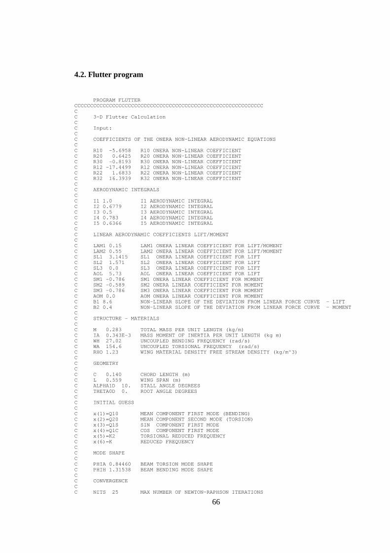
66

4.2. Flutter program

PROGRAM FLUTTER CCCCCCCCCCCCCCCCCCCCCCCCCCCCCCCCCCCCCCCCCCCCCCCCCCCCCCCCCCCC C C 3- D Fl ut t er Cal cul at i on C C I nput : C C COEFFI CI ENTS OF THE ONERA NON- LI NEAR AERODYNAMI C EQUATI ONS C C R10 - 5. 6958 R10 ONERA NON- LI NEAR COEFFI CI ENT C R20 0. 6425 R20 ONERA NON- LI NEAR COEFFI CI ENT C R30 - 0. 8193 R30 ONERA NON- LI NEAR COEFFI CI ENT C R12 - 17. 4499 R12 ONERA NON- LI NEAR COEFFI CI ENT C R22 1. 6833 R22 ONERA NON- LI NEAR COEFFI CI ENT C R32 16. 3939 R32 ONERA NON- LI NEAR COEFFI CI ENT C C AERODYNAMI C I NTEGRALS C C I 1 1. 0 I 1 AERODYNAMI C I NTEGRAL C I 2 0. 6779 I 2 AERODYNAMI C I NTEGRAL C I 3 0. 5 I 3 AERODYNAMI C I NTEGRAL C I 4 0. 783 I 4 AERODYNAMI C I NTEGRAL C I 5 0. 6366 I 5 AERODYNAMI C I NTEGRAL C C LI NEAR AERODYNAMI C COEFFI CI ENTS LI FT/ MOMENT C C LAM1 0. 15 LAM1 ONERA LI NEAR COEFFI CI ENT FOR LI FT/ MOMENT C LAM2 0. 55 LAM2 ONERA LI NEAR COEFFI CI ENT FOR LI FT/ MOMENT C SL1 3. 1415 SL1 ONERA LI NEAR COEFFI CI ENT FOR LI FT C SL2 1. 571 SL2 ONERA LI NEAR COEFFI CI ENT FOR LI FT C SL3 0. 0 SL3 ONERA LI NEAR COEFFI CI ENT FOR LI FT C AOL 5. 73 AOL ONERA LI NEAR COEFFI CI ENT FOR LI FT C SM1 - 0. 786 SM1 ONERA LI NEAR COEFFI CI ENT FOR MOMENT C SM2 - 0. 589 SM2 ONERA LI NEAR COEFFI CI ENT FOR MOMENT C SM3 - 0. 786 SM3 ONERA LI NEAR COEFFI CI ENT FOR MOMENT C AOM 0. 0 AOM ONERA LI NEAR COEFFI CI ENT FOR MOMENT C B1 8. 6 NON- LI NEAR SLOPE OF THE DEVI ATI ON FROM LI NEAR FORCE CURVE - LI FT C B2 0. 4 NON- LI NEAR SLOPE OF THE DEVI ATI ON FROM LI NEAR FORCE CURVE - MOMENT C C STRUCTURE - MATERI ALS C C M 0. 283 TOTAL MASS PER UNI T LENGTH ( kg/ m) C I A 0. 343E- 3 MASS MOMENT OF I NERTI A PER UNI T LENGTH ( kg m) C WH 27. 02 UNCOUPLED BENDI NG FREQUENCY ( r ad/ s) C WA 154. 6 UNCOUPLED TORSI ONAL FREQUENCY ( r ad/ s) C RHO 1. 23 WI NG MATERI AL DENSI TY FREE STREAM DENSI TY ( kg/ m̂ 3) C C GEOMETRY C C C 0. 140 CHORD LENGTH ( m) C L 0. 559 WI NG SPAN ( m) C ALPHA1D 10. STALL ANGLE DEGREES C THETA0D 0. ROOT ANGLE DEGREES C C I NI TI AL GUESS C C x( 1) =Q10 MEAN COMPONENT FI RST MODE ( BENDI NG) C x( 2) =Q20 MEAN COMPONENT SECOND MODE ( TORSI ON) C x( 3) =Q1S SI N COMPONENT FI RST MODE C x( 4) =Q1C COS COMPONENT FI RST MODE C x( 5) =K2 TORSI ONAL REDUCED FREQUENCY C x( 6) =K REDUCED FREQUENCY C C MODE SHAPE C C PHI A 0. 84460 BEAM TORSI ON MODE SHAPE C PHI H 1. 31538 BEAM BENDI NG MODE SHAPE C C CONVERGENCE C C NI TS 25 MAX NUMBER OF NEWTON- RAPHSON I TERATI ONS

67

C TOLER 1. E- 4 TOLERANCE FOR EACH OF THE 6 UNKNOWNS C C PARAMETERI C STUDY C C Q2C 0. 0 COS COMPONENT OF THE SECOND MODAL FORCE C Q2S 0. 1 SI NE COMPONENT OF THE SECOND MODAL FORCE C CCCCCCCCCCCCCCCCCCCCCCCCCCCCCCCCCCCCCCCCCCCCCCCCCCCCCCCCCCCC PARAMETER ( NN=6) I NTEGER N, NP, I , T, J, I NDX( NN) , NI TS REAL* 8 1 X( 1: NN) , FVEC( 1: NN) , FJAC( 1: NN, 1: NN) , DELTA( NN) , FS, FQ, AVI B, 2 ALPHA0, PHI 1T, PHI 1, TOLER REAL Y( NN, NN) , D, THETA0, THETA0D, Q2S C REAL 1 R10, R20, R30, R12, R22, R32, 2 I 1, I 2, I 3, I 4, I 5, 3 LAM1, LAM2, SL1, SL2, SL3, AOL, SM1, SM2, SM3, AOM, B1, B2, 4 M, I A, RHO, C, L, WH, WA, ALPHA1D, ALPHA1, ALPHA1T, B, PI , OM, MU, RA, 5 PHI A, PHI H, Q2C COMMON/ USER/ 1 R10, R20, R30, R12, R22, R32, 2 I 1, I 2, I 3, I 4, I 5, 3 LAM1, LAM2, SL1, SL2, SL3, AOL, SM1, SM2, SM3, AOM, B1, B2, 4 M, I A, RHO, C, L, WH, WA, ALPHA1D, ALPHA1, ALPHA1T, B, PI , OM, MU, RA, 5 PHI A, PHI H, Q2C C C READ DATA FROM THE I NPUT FI LE C OPEN ( 10, FI LE=' aer oel 3. i n' , STATUS=' OLD' ) READ ( 10, 120) R10, R20, R30, R12, R22, R32 READ ( 10, 120) I 1, I 2, I 3, I 4, I 5 READ ( 10, 120) LAM1, LAM2, SL1, SL2, SL3, AOL, SM1, SM2, SM3, AOM, B1, B2 READ ( 10, 120) M, I A, RHO, C, L, WH, WA, ALPHA1D, THETA0D READ ( 10, 120) X( 1) , X( 2) , X( 3) , X( 4) , X( 5) , X( 6) READ ( 10, 120) PHI A, PHI H READ ( 10, * ) NI TS READ ( 10, 120) TOLER READ ( 10, 120) Q2C, Q2S C C CREATE OUTPUT FI LE C OPEN ( 9, FI LE=' aer oel 3. out ' , STATUS=' UNKNOWN' ) WRI TE ( 9, * ) WRI TE ( 9, * ) ' # 3D Fl ut t er Cal cul at i on' WRI TE ( 9, * ) WRI TE ( 9, 105) 1 ' Q2S' , ' Q10' , ' Q20' , ' Q1S' , ' Q1C' , ' K2' , ' K' , 2 ' FS ( M/ S) ' , ' W ( Hz) ' , ' A0' , ' AV' C C SETUP PARAMETERS C THETA0=DEG2RAD( THETA0D) N=6 NP=6 C ALPHA1=DEG2RAD( ALPHA1D) ALPHA1T=- ALPHA1 B=0. 5* C PI =3. 14159 OM=WH/ WA MU=( M/ L) / ( PI * RHO* B* B) RA=SQRT( I A/ M) / B C C NEWTON STEP C T=0 DO I =1, N DELTA( I ) =5. ENDDO 20 CONTI NUE pr i nt * , ' START' , T I F ( DABS( DELTA( 1) ) . LE. TOLER. AND. 1 DABS( DELTA( 2) ) . LE. TOLER. AND. 2 DABS( DELTA( 3) ) . LE. TOLER. AND. 3 DABS( DELTA( 4) ) . LE. TOLER. AND. 4 DABS( DELTA( 5) ) . LE. TOLER. AND.

68

5 DABS( DELTA( 6) ) . LE. TOLER) GOTO 90 T=T+1 C C CALCULATE THE FUNCTI ONS USI NG THE I NI TI AL VALUES FOR THE C STATE VECTOR X C CALL FUNCV( THETA0, Q2S, ALPHA0, AVI B, PHI 1, PHI 1T, N, X, FVEC) C C CALCULATE THE JACOBI AN MATRI X C CALL FDJAC( Q2S, THETA0, N, X, FVEC, NP, FJAC) C DO I =1, N DO J=1, N Y( I , J) =0. ENDDO Y( I , I ) =1. ENDDO C C CALCULATE THE I NVERSE OF THE JACOBI AN MATRI X C CALL LUDCMP ( FJAC, N, NP, I NDX, D) DO J=1, N CALL LUBKSB ( FJAC, N, NP, I NDX, Y( 1, J) ) ENDDO C C CALCULATE DELTA C DO J=1, N DELTA( J) =0. DO I =1, N DELTA( J) =DELTA( J) +Y( J, I ) * FVEC( I ) ENDDO ENDDO C C CALCULATE X AT THE NEXT I TERATI ON C DO I =1, N X( I ) =X( I ) - DELTA( I ) ENDDO C I F ( T. LT. NI TS) GOTO 20 C C PRI NTOUT C CONTI NUE pr i nt * , T I F ( T. GT. NI TS) THEN WRI TE ( * , * ) ' DI VERGENCE' STOP ENDI F C C CALCULATE FLUTTER VELOCI TY AND FREQUENCY C 90 FS=WA* B/ X( 5) FQ=FS* X( 6) / ( B* 2. * PI ) WRI TE ( 9, 110) 1 Q2S, X( 1) , X( 2) , X( 3) , X( 4) , X( 5) , X( 6) , 2 FS, FQ, RAD2DEG( ALPHA0) , RAD2DEG( AVI B) C C NEXT Q2S ENTRY C DO I =1, N X( I ) =X( I ) +0. 0001 ENDDO READ ( 10, * ) Q2S T=0 DO I =1, N DELTA( I ) =5. ENDDO I F ( Q2S. LT. 999. 0) GOTO 20 C STOP C C FORMAT STATEMENTS C 105 FORMAT( ' #' , 11( 1X, A11) ) 110 FORMAT( 11( 1X, F11. 4) )

69

120 FORMAT( 1X, F10. 5) END CCCCCCCCCCCCCCCCCCCCCCCCCCCCCCCCCCCCCCCCCCCCCCCCCCCCCCCCCCCC SUBROUTI NE FDJAC ( Q2S, THETA0, N, X, FVEC, NP, DF) C C THE JACOBI AN MATRI X I S CALCULATED I NCREASI NG THE STATE VECTOR C BY A SMALL NUMBER CCCCCCCCCCCCCCCCCCCCCCCCCCCCCCCCCCCCCCCCCCCCCCCCCCCCCCCCCCCC REAL* 8 DF( NP, NP) , FVEC( N) , X( N) , EPS, F( 40) , ALPHA0, AVI B, PHI 1, PHI 1T REAL H, TEMP, THETA0 EPS=1. E- 4 DO J=1, N TEMP=X( J) H=EPS* ABS( TEMP) I F ( H. EQ. 0. ) H=EPS X( J) =TEMP+H H=X( J) - TEMP CALL FUNCV ( THETA0, Q2S, ALPHA0, AVI B, PHI 1, PHI 1T, N, X, F) X( J) =TEMP DO I =1, N DF( I , J) =( F( I ) - FVEC( I ) ) / H ENDDO ENDDO C RETURN END CCCCCCCCCCCCCCCCCCCCCCCCCCCCCCCCCCCCCCCCCCCCCCCCCCCCCCCCCCCC SUBROUTI NE FUNCV ( THETA0, Q2S, ALPHA0, AVI B, PHI 1, PHI 1T, N, X, P) C C THE AEROELASTI C MODEL I S USED HERE TO FORMULATE THE EQUATI ONS C WHI CH ARE TO BE SOLVED ( P) . THE VARI ABLES CAN BE EASI LY I DENTI FI ED C WI TH THE NAME OF THE VARI ABLES I N THE DI SSERTATI ON. CCCCCCCCCCCCCCCCCCCCCCCCCCCCCCCCCCCCCCCCCCCCCCCCCCCCCCCCCCCC I NTEGER N REAL Q2S, THETA0 REAL* 8 X( N) , P( N) , CL20, CM20, ALPHA0, ALPHAS, ALPHAC, AVI B, F, G, 1BOL, B1L, B2L, B3L, B4L, BOM, B1M, B2M, B3M, B4M, PENT, PENT2, PHI 1, PHI 1T, 2DCL0, DCLS1, R1L, R2L, R3L, K1L, K2L, RS1L, RC1L, ALS1, BLC1, DCM0, DCMS1, R1M, 3R2M, R3M, K1M, K2M, RS1M, RC1M, AMS1, BMC1 C REAL 1 R10, R20, R30, R12, R22, R32, 2 I 1, I 2, I 3, I 4, I 5, 3 LAM1, LAM2, SL1, SL2, SL3, AOL, SM1, SM2, SM3, AOM, B1, B2, 4 M, I A, RHO, C, L, WH, WA, ALPHA1D, ALPHA1, ALPHA1T, B, PI , OM, MU, RA, 5 PHI A, PHI H, Q2C COMMON/ USER/ 1 R10, R20, R30, R12, R22, R32, 2 I 1, I 2, I 3, I 4, I 5, 3 LAM1, LAM2, SL1, SL2, SL3, AOL, SM1, SM2, SM3, AOM, B1, B2, 4 M, I A, RHO, C, L, WH, WA, ALPHA1D, ALPHA1, ALPHA1T, B, PI , OM, MU, RA, 5 PHI A, PHI H, Q2C C C ANGLE OF ATTACK I N STRUCTURAL CO- ORDI NATES C ALPHA0=THETA0+. 5* PHI A* X( 2) ALPHAS=PHI A* ( . 5* Q2S+. 25* X( 6) * Q2C) +PHI H* X( 6) * X( 4) ALPHAC=PHI A* ( . 5* Q2C- . 25* X( 6) * Q2S) - PHI H* X( 6) * X( 3) AVI B=DSQRT( ALPHAS* ALPHAS+ALPHAC* ALPHAC) C C LI NEAR PART - L REFERS TO LI FT C F=( X( 6) * X( 6) * LAM2+LAM1* LAM1) / ( LAM1* LAM1+X( 6) * X( 6) ) G=( X( 6) * LAM1* ( LAM2- 1) ) / ( LAM1* LAM1+X( 6) * X( 6) ) BOL=X( 2) * AOL* . 5 B1L=X( 6) * ( . 25* X( 6) * SL1- . 5* X( 6) * SL2- . 25* G* AOL) +. 5* F* AOL B2L=X( 6) * ( . 5* SL1+. 5* SL3+. 25* F* AOL) +. 5* G* AOL B3L=X( 6) * ( SL1* X( 6) +G* AOL) B4L=F* AOL* X( 6) C C LI NEAR PART - M REFERS TO MOMENT C BOM=X( 2) * AOM* . 5 B1M=X( 6) * ( . 25* X( 6) * SM1- . 5* X( 6) * SM2- . 25* G* AOM) +. 5* F* AOM B2M=X( 6) * ( 0. 5* SM1+0. 5* SM3+0. 25* F* AOM) +. 5* G* AOM B3M=X( 6) * ( SM1* X( 6) +G* AOM) B4M=F* AOM* X( 6) C

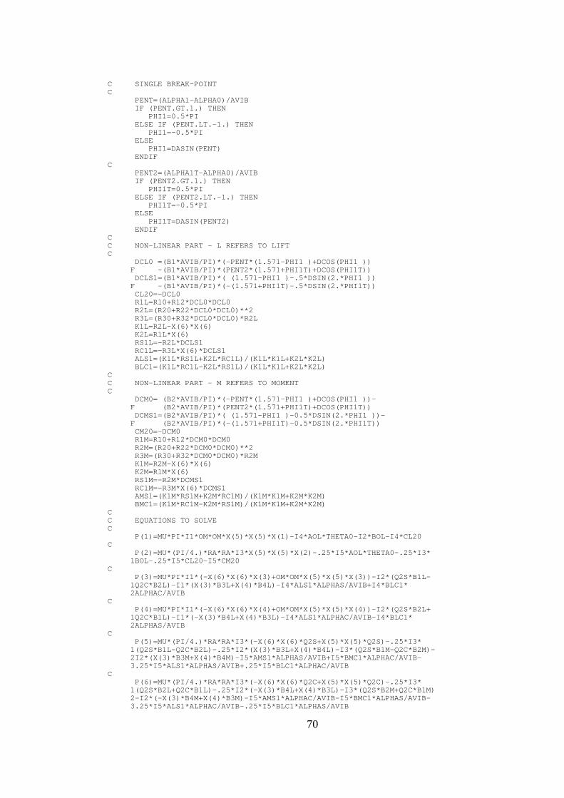
70

C SI NGLE BREAK- POI NT C PENT=( ALPHA1- ALPHA0) / AVI B I F ( PENT. GT. 1. ) THEN PHI 1=0. 5* PI ELSE I F ( PENT. LT. - 1. ) THEN PHI 1=- 0. 5* PI ELSE PHI 1=DASI N( PENT) ENDI F C PENT2=( ALPHA1T- ALPHA0) / AVI B I F ( PENT2. GT. 1. ) THEN PHI 1T=0. 5* PI ELSE I F ( PENT2. LT. - 1. ) THEN PHI 1T=- 0. 5* PI ELSE PHI 1T=DASI N( PENT2) ENDI F C C NON- LI NEAR PART - L REFERS TO LI FT C DCL0 =( B1* AVI B/ PI ) * ( - PENT* ( 1. 571- PHI 1 ) +DCOS( PHI 1 ) ) F - ( B1* AVI B/ PI ) * ( PENT2* ( 1. 571+PHI 1T) +DCOS( PHI 1T) ) DCLS1=( B1* AVI B/ PI ) * ( ( 1. 571- PHI 1 ) - . 5* DSI N( 2. * PHI 1 ) ) F - ( B1* AVI B/ PI ) * ( - ( 1. 571+PHI 1T) - . 5* DSI N( 2. * PHI 1T) ) CL20=- DCL0 R1L=R10+R12* DCL0* DCL0 R2L=( R20+R22* DCL0* DCL0) * * 2 R3L=( R30+R32* DCL0* DCL0) * R2L K1L=R2L- X( 6) * X( 6) K2L=R1L* X( 6) RS1L=- R2L* DCLS1 RC1L=- R3L* X( 6) * DCLS1 ALS1=( K1L* RS1L+K2L* RC1L) / ( K1L* K1L+K2L* K2L) BLC1=( K1L* RC1L- K2L* RS1L) / ( K1L* K1L+K2L* K2L) C C NON- LI NEAR PART - M REFERS TO MOMENT C DCM0= ( B2* AVI B/ PI ) * ( - PENT* ( 1. 571- PHI 1 ) +DCOS( PHI 1 ) ) - F ( B2* AVI B/ PI ) * ( PENT2* ( 1. 571+PHI 1T) +DCOS( PHI 1T) ) DCMS1=( B2* AVI B/ PI ) * ( ( 1. 571- PHI 1 ) - 0. 5* DSI N( 2. * PHI 1 ) ) - F ( B2* AVI B/ PI ) * ( - ( 1. 571+PHI 1T) - 0. 5* DSI N( 2. * PHI 1T) ) CM20=- DCM0 R1M=R10+R12* DCM0* DCM0 R2M=( R20+R22* DCM0* DCM0) * * 2 R3M=( R30+R32* DCM0* DCM0) * R2M K1M=R2M- X( 6) * X( 6) K2M=R1M* X( 6) RS1M=- R2M* DCMS1 RC1M=- R3M* X( 6) * DCMS1 AMS1=( K1M* RS1M+K2M* RC1M) / ( K1M* K1M+K2M* K2M) BMC1=( K1M* RC1M- K2M* RS1M) / ( K1M* K1M+K2M* K2M) C C EQUATI ONS TO SOLVE C P( 1) =MU* PI * I 1* OM* OM* X( 5) * X( 5) * X( 1) - I 4* AOL* THETA0- I 2* BOL- I 4* CL20 C P( 2) =MU* ( PI / 4. ) * RA* RA* I 3* X( 5) * X( 5) * X( 2) - . 25* I 5* AOL* THETA0- . 25* I 3* 1BOL- . 25* I 5* CL20- I 5* CM20 C P( 3) =MU* PI * I 1* ( - X( 6) * X( 6) * X( 3) +OM* OM* X( 5) * X( 5) * X( 3) ) - I 2* ( Q2S* B1L- 1Q2C* B2L) - I 1* ( X( 3) * B3L+X( 4) * B4L) - I 4* ALS1* ALPHAS/ AVI B+I 4* BLC1* 2ALPHAC/ AVI B C P( 4) =MU* PI * I 1* ( - X( 6) * X( 6) * X( 4) +OM* OM* X( 5) * X( 5) * X( 4) ) - I 2* ( Q2S* B2L+ 1Q2C* B1L) - I 1* ( - X( 3) * B4L+X( 4) * B3L) - I 4* ALS1* ALPHAC/ AVI B- I 4* BLC1* 2ALPHAS/ AVI B C P( 5) =MU* ( PI / 4. ) * RA* RA* I 3* ( - X( 6) * X( 6) * Q2S+X( 5) * X( 5) * Q2S) - . 25* I 3* 1( Q2S* B1L- Q2C* B2L) - . 25* I 2* ( X( 3) * B3L+X( 4) * B4L) - I 3* ( Q2S* B1M- Q2C* B2M) - 2I 2* ( X( 3) * B3M+X( 4) * B4M) - I 5* AMS1* ALPHAS/ AVI B+I 5* BMC1* ALPHAC/ AVI B- 3. 25* I 5* ALS1* ALPHAS/ AVI B+. 25* I 5* BLC1* ALPHAC/ AVI B C P( 6) =MU* ( PI / 4. ) * RA* RA* I 3* ( - X( 6) * X( 6) * Q2C+X( 5) * X( 5) * Q2C) - . 25* I 3* 1( Q2S* B2L+Q2C* B1L) - . 25* I 2* ( - X( 3) * B4L+X( 4) * B3L) - I 3* ( Q2S* B2M+Q2C* B1M) 2- I 2* ( - X( 3) * B4M+X( 4) * B3M) - I 5* AMS1* ALPHAC/ AVI B- I 5* BMC1* ALPHAS/ AVI B- 3. 25* I 5* ALS1* ALPHAC/ AVI B- . 25* I 5* BLC1* ALPHAS/ AVI B

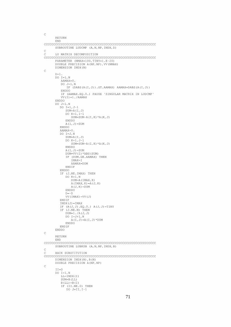
71

C RETURN END CCCCCCCCCCCCCCCCCCCCCCCCCCCCCCCCCCCCCCCCCCCCCCCCCCCCCCCCCCCC SUBROUTI NE LUDCMP ( A, N, NP, I NDX, D) C C LU MATRI X DECOMPOSI TI ON CCCCCCCCCCCCCCCCCCCCCCCCCCCCCCCCCCCCCCCCCCCCCCCCCCCCCCCCCCCC PARAMETER ( NMAX=100, TI NY=1. E- 20) DOUBLE PRECI SI ON A( NP, NP) , VV( NMAX) DI MENSI ON I NDX( N) C D=1. DO I =1, N AAMAX=0. DO J=1, N I F ( DABS( A( I , J) ) . GT. AAMAX) AAMAX=DABS( A( I , J) ) ENDDO I F ( AAMAX. EQ. 0. ) PAUSE ' SI NGULAR MATRI X I N LUDCMP' VV( I ) =1. / AAMAX ENDDO DO J=1, N DO I =1, J- 1 SUM=A( I , J) DO K=1, I - 1 SUM=SUM- A( I , K) * A( K, J) ENDDO A( I , J) =SUM ENDDO AAMAX=0. DO I =J, N SUM=A( I , J) DO K=1, J- 1 SUM=SUM- A( I , K) * A( K, J) ENDDO A( I , J) =SUM DUM=VV( I ) * ABS( SUM) I F ( DUM. GE. AAMAX) THEN I MAX=I AAMAX=DUM ENDI F ENDDO I F ( J. NE. I MAX) THEN DO K=1, N DUM=A( I MAX, K) A( I MAX, K) =A( J, K) A( J, K) =DUM ENDDO D=- D VV( I MAX) =VV( J) ENDI F I NDX( J) =I MAX I F ( A( J, J) . EQ. 0. ) A( J, J) =TI NY I F ( J. NE. N) THEN DUM=1. / A( J, J) DO I =J+1, N A( I , J) =A( I , J) * DUM ENDDO ENDI F ENDDO C RETURN END CCCCCCCCCCCCCCCCCCCCCCCCCCCCCCCCCCCCCCCCCCCCCCCCCCCCCCCCCCCC SUBROUTI NE LUBKSB ( A, N, NP, I NDX, B) C C BACK SUBSTI TUTI ON CCCCCCCCCCCCCCCCCCCCCCCCCCCCCCCCCCCCCCCCCCCCCCCCCCCCCCCCCCCC DI MENSI ON I NDX( N) , B( N) DOUBLE PRECI SI ON A( NP, NP) C I I =0 DO I =1, N LL=I NDX( I ) SUM=B( LL) B( LL) =B( I ) I F ( I I . NE. 0) THEN DO J=I I , I - 1

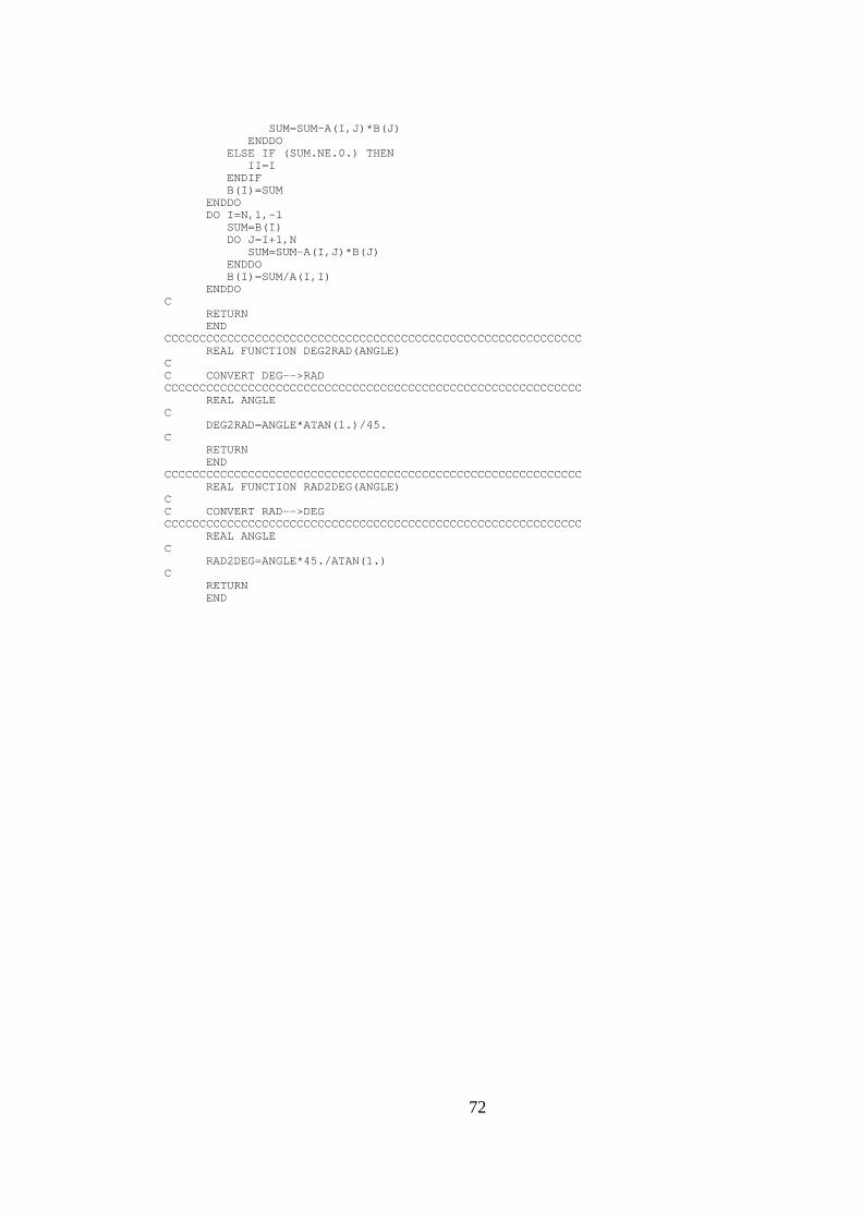
72

SUM=SUM- A( I , J) * B( J) ENDDO ELSE I F ( SUM. NE. 0. ) THEN I I =I ENDI F B( I ) =SUM ENDDO DO I =N, 1, - 1 SUM=B( I ) DO J=I +1, N SUM=SUM- A( I , J) * B( J) ENDDO B( I ) =SUM/ A( I , I ) ENDDO C RETURN END CCCCCCCCCCCCCCCCCCCCCCCCCCCCCCCCCCCCCCCCCCCCCCCCCCCCCCCCCCCC REAL FUNCTI ON DEG2RAD( ANGLE) C C CONVERT DEG- - >RAD CCCCCCCCCCCCCCCCCCCCCCCCCCCCCCCCCCCCCCCCCCCCCCCCCCCCCCCCCCCC REAL ANGLE C DEG2RAD=ANGLE* ATAN( 1. ) / 45. C RETURN END CCCCCCCCCCCCCCCCCCCCCCCCCCCCCCCCCCCCCCCCCCCCCCCCCCCCCCCCCCCC REAL FUNCTI ON RAD2DEG( ANGLE) C C CONVERT RAD- - >DEG CCCCCCCCCCCCCCCCCCCCCCCCCCCCCCCCCCCCCCCCCCCCCCCCCCCCCCCCCCCC REAL ANGLE C RAD2DEG=ANGLE* 45. / ATAN( 1. ) C RETURN END

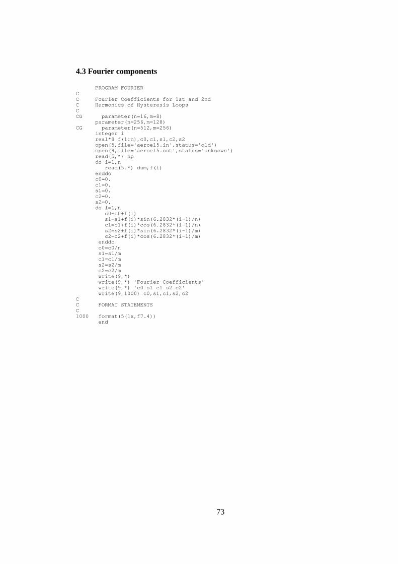
73

4.3 Fourier components PROGRAM FOURI ER C C Four i er Coef f i c i ent s f or 1st and 2nd C Har moni cs of Hyst er esi s Loops C CG par amet er ( n=16, m=8) par amet er ( n=256, m=128) CG par amet er ( n=512, m=256) i nt eger i r eal * 8 f ( 1: n) , c0, c1, s1, c2, s2 open( 5, f i l e=' aer oel 5. i n' , st at us=' ol d' ) open( 9, f i l e=' aer oel 5. out ' , st at us=' unknown' ) r ead( 5, * ) np do i =1, n r ead( 5, * ) dum, f ( i ) enddo c0=0. c1=0. s1=0. c2=0. s2=0. do i =1, n c0=c0+f ( i ) s1=s1+f ( i ) * si n( 6. 2832* ( i - 1) / n) c1=c1+f ( i ) * cos( 6. 2832* ( i - 1) / n) s2=s2+f ( i ) * si n( 6. 2832* ( i - 1) / m) c2=c2+f ( i ) * cos( 6. 2832* ( i - 1) / m) enddo c0=c0/ n s1=s1/ m c1=c1/ m s2=s2/ m c2=c2/ m wr i t e( 9, * ) wr i t e( 9, * ) ' Four i er Coef f i c i ent s ' wr i t e( 9, * ) ' c0 s1 c1 s2 c2' wr i t e( 9, 1000) c0, s1, c1, s2, c2 C C FORMAT STATEMENTS C 1000 f or mat ( 5( 1x, f 7. 4) ) end

74

4.4 Flutter Divergence PROGRAM DI VERGENCE CCCCCCCCCCCCCCCCCCCCCCCCCCCCCCCCCCCCCCCCCCCCCCCCCCCCCCCCCCCC C STATI C DI VERGENCE CALCULATI ON C C I nput : C C AERODYNAMI C I NTEGRALS C C I 1 1. 0 I 1 AERODYNAMI C I NTEGRAL C I 2 0. 6779 I 2 AERODYNAMI C I NTEGRAL C I 3 0. 5 I 3 AERODYNAMI C I NTEGRAL C I 4 0. 783 I 4 AERODYNAMI C I NTEGRAL C I 5 0. 6366 I 5 AERODYNAMI C I NTEGRAL C C LI NEAR AERODYNAMI C COEFFI CI ENTS LI FT/ MOMENT C C AOL 5. 73 AOL ONERA LI NEAR COEFFI CI ENT FOR LI FT C B1 8. 6 NON- LI NEAR SLOPE OF THE DEVI ATI ON FROM LI NEAR FORCE CURVE - LI FT C B2 0. 4 NON- LI NEAR SLOPE OF THE DEVI ATI ON FROM LI NEAR FORCE CURVE - MOMENT C C STRUCTURE - MATERI ALS C C M 0. 283 TOTAL MASS PER UNI T LENGTH ( kg/ m) C I A 0. 343E- 3 MASS MOMENT OF I NERTI A PER UNI T LENGTH ( kg m) C WH 27. 02 UNCOUPLED BENDI NG FREQUENCY ( r ad/ s) C WA 154. 6 UNCOUPLED TORSI ONAL FREQUENCY ( r ad/ s) C RHO 1. 23 WI NG MATERI AL DENSI TY FREE STREAM DENSI TY ( kg/ m̂ 3) C C GEOMETRY C C C 0. 140 CHORD LENGTH ( m) C L 0. 559 WI NG SPAN ( m) C ALPHA1D 10. STALL ANGLE DEGREES C THETA0D 0. ROOT ANGLE DEGREES C C I NI TI AL GUESS C C x( 1) =Q10 MEAN COMPONENT FI RST MODE ( BENDI NG) C x( 2) =Q20 MEAN COMPONENT SECOND MODE ( TORSI ON) C C MODE SHAPE C C PHI A 0. 84460 BEAM TORSI ON MODE SHAPE C C CONVERGENCE C C NI TS 25 MAX NUMBER OF NEWTON- RAPHSON I TERATI ONS C TOLER 1. E- 4 TOLERANCE FOR EACH OF THE 6 UNKNOWNS C C PARAMETERI C STUDY C C Q2S 0. 1 SI NE COMPONENT OF THE SECOND MODAL FORCE C CCCCCCCCCCCCCCCCCCCCCCCCCCCCCCCCCCCCCCCCCCCCCCCCCCCCCCCCCCCC PARAMETER ( NN=2) I NTEGER N, NP, I , T, J, I NDX( NN) , NI TS REAL* 8 1 X( 1: NN) , FVEC( 1: NN) , FJAC( 1: NN, 1: NN) , DELTA( NN) , 2 ALPHA0, PHI 1, TOLER REAL Y( NN, NN) , D, THETA0, THETA0D, KAT C REAL 1 I 1, I 2, I 3, I 4, I 5, AOL, B1, B2, PHI A, AVI BD, AVI B, 2 M, I A, RHO, C, L, WH, WA, ALPHA1D, ALPHA1, B, PI , OM, MU, RA COMMON/ USER/ 1 I 1, I 2, I 3, I 4, I 5, AOL, B1, B2, PHI A, AVI BD, AVI B, 2 M, I A, RHO, C, L, WH, WA, ALPHA1D, ALPHA1, B, PI , OM, MU, RA C C READ DATA FROM THE I NPUT FI LE C OPEN ( 10, FI LE=' aer oel 6. i n' , STATUS=' OLD' ) READ ( 10, 120) I 1, I 2, I 3, I 4, I 5, AOL, B1, B2 READ ( 10, 120) M, I A, RHO, C, L, WH, WA, ALPHA1D, THETA0D

75

READ ( 10, 120) X( 1) , X( 2) , PHI A, AVI BD READ ( 10, * ) NI TS READ ( 10, 120) TOLER, KAT C C CREATE OUTPUT FI LE C OPEN ( 9, FI LE=' aer oel 6. out ' , STATUS=' UNKNOWN' ) WRI TE ( 9, * ) WRI TE ( 9, * ) ' # Cal cul at i on of Fl ut t er Di ver gence' WRI TE ( 9, * ) WRI TE ( 9, 105) 1 ' Thet a- R' , ' K2' , ' Q10' , ' Q20' , ' AOA( deg) ' , ' V( m/ 2) ' C C SETUP PARAMETERS C THETA0=DEG2RAD( THETA0D) AVI B =DEG2RAD( AVI BD) N=2 NP=2 ALPHA1=DEG2RAD( ALPHA1D) B=0. 5* C PI =3. 14159 OM=WH/ WA MU=( M/ L) / ( PI * RHO* B* B) RA=SQRT( I A/ M) / B C C NEWTON STEP C T=0 DO I =1, N DELTA( I ) =5. ENDDO 20 CONTI NUE pr i nt * , ' START' , T I F ( DABS( DELTA( 1) ) . LE. TOLER. AND. 2 DABS( DELTA( 2) ) . LE. TOLER) GOTO 90 T=T+1 C C CALCULATE THE FUNCTI ONS USI NG THE I NI TI AL VALUES FOR THE C STATE VECTOR X C CALL FUNCV( KAT, THETA0, N, X, FVEC) C C CALCULATE THE JACOBI AN MATRI X C CALL FDJAC( KAT, THETA0, N, X, FVEC, NP, FJAC) C DO I =1, N DO J=1, N Y( I , J) =0. ENDDO Y( I , I ) =1. ENDDO C C CALCULATE THE I NVERSE OF THE JACOBI AN MATRI X C CALL LUDCMP ( FJAC, N, NP, I NDX, D) DO J=1, N CALL LUBKSB ( FJAC, N, NP, I NDX, Y( 1, J) ) ENDDO C C CALCULATE DELTA C DO J=1, N DELTA( J) =0. DO I =1, N DELTA( J) =DELTA( J) +Y( J, I ) * FVEC( I ) ENDDO ENDDO C C CALCULATE X AT THE NEXT I TERATI ON C DO I =1, N X( I ) =X( I ) - DELTA( I ) ENDDO C I F ( T. LT. NI TS) GOTO 20 C

76

C PRI NTOUT C CONTI NUE pr i nt * , T I F ( T. GT. NI TS) THEN WRI TE ( * , * ) ' DI VERGENCE' STOP ENDI F C C CALCULATE FLUTTER VELOCI TY AND FREQUENCY C 90 V=WA* B/ KAT AOA=THETA0+0. 5* PHI A* X( 2) WRI TE ( 9, 110) THETA0, KAT, X( 1) , X( 2) , RAD2DEG( AOA) , V C C NEXT KAT ENTRY C T=0 DO I =1, N X( I ) =X( I ) +0. 0001 ENDDO DO I =1, N DELTA( I ) =5. ENDDO READ ( 10, * ) KAT I F ( KAT. LT. 999. 0) GOTO 20 C STOP C C FORMAT STATEMENTS C 105 FORMAT( ' #' , 11( 1X, A11) ) 110 FORMAT( 11( 1X, F11. 4) ) 120 FORMAT( 1X, F10. 5) END CCCCCCCCCCCCCCCCCCCCCCCCCCCCCCCCCCCCCCCCCCCCCCCCCCCCCCCCCCCC SUBROUTI NE FDJAC ( KAT, THETA0, N, X, FVEC, NP, DF) C C THE JACOBI AN MATRI X I S CALCULATED I NCREASI NG C THE STATE VECTOR BY A SMALL NUMBER CCCCCCCCCCCCCCCCCCCCCCCCCCCCCCCCCCCCCCCCCCCCCCCCCCCCCCCCCCCC PARAMETER ( NMAX=40) I NTEGER N, NP, NMAX REAL* 8 DF( NP, NP) , FVEC( N) , X( N) , EPS, F( NMAX) I NTEGER I , J REAL H, TEMP, THETA0, KAT EPS=1. E- 4 DO J=1, N TEMP=X( J) H=EPS* ABS( TEMP) I F ( H. EQ. 0. ) H=EPS X( J) =TEMP+H H=X( J) - TEMP CALL FUNCV ( KAT, THETA0, N, X, F) X( J) =TEMP DO I =1, N DF( I , J) =( F( I ) - FVEC( I ) ) / H ENDDO ENDDO C RETURN END CCCCCCCCCCCCCCCCCCCCCCCCCCCCCCCCCCCCCCCCCCCCCCCCCCCCCCCCCCCC SUBROUTI NE FUNCV ( KAT, THETA0, N, X, P) C C THE AEROELASTI C MODEL I S USED HERE TO FORMULATE THE EQUATI ONS C WHI CH ARE TO BE SOLVED ( P) . THE VARI ABLES CAN BE EASI LY I DENTI FI ED C WI TH THE NAME OF THE VARI ABLES I N THE DI SSERTATI ON. CCCCCCCCCCCCCCCCCCCCCCCCCCCCCCCCCCCCCCCCCCCCCCCCCCCCCCCCCCCC I NTEGER N REAL Q2S, THETA0, KAT REAL* 8 X( N) , P( N) , CL20, CM20, ALPHA0, BOL, PENT, PHI 1 C REAL 1 I 1, I 2, I 3, I 4, I 5, AOL, B1, B2, PHI A, AVI BD, AVI B, 2 M, I A, RHO, C, L, WH, WA, ALPHA1D, ALPHA1, B, PI , OM, MU, RA COMMON/ USER/ 1 I 1, I 2, I 3, I 4, I 5, AOL, B1, B2, PHI A, AVI BD, AVI B,

77

2 M, I A, RHO, C, L, WH, WA, ALPHA1D, ALPHA1, B, PI , OM, MU, RA C C ANGLE OF ATTACK I N STRUCTURAL CO- ORDI NATES C ALPHA0=THETA0+. 5* PHI A* X( 2) C C SI NGLE BREAK- POI NT C PENT=( ALPHA1- ALPHA0) / AVI B I F ( PENT. GT. 1. ) THEN PHI 1=0. 5* PI ELSE I F ( PENT. LT. - 1. ) THEN PHI 1=- 0. 5* PI ELSE PHI 1=DASI N( PENT) ENDI F C C NON- LI NEAR PART - L REFERS TO LI FT C CL20=- ( B1* AVI B/ PI ) * ( - PENT* ( 1. 571- PHI 1 ) +DCOS( PHI 1 ) ) C C NON- LI NEAR PART - M REFERS TO MOMENT C CM20=- ( B2* AVI B/ PI ) * ( - PENT* ( 1. 571- PHI 1 ) +DCOS( PHI 1 ) ) C C EQUATI ONS TO SOLVE C B0L=0. 25* A0L* X( 2) P( 1) =MU* PI * I 1* OM* OM* KAT* X( 1) - I 4* AOL* THETA0- I 2* BOL- I 4* CL20 C P( 2) =MU* ( PI / 4. ) * RA* RA* I 3* kat * kat * X( 2) - . 25* I 5* AOL* THETA0 1 - 0. 25* I 3* BOL- 0. 25* I 5* CL20- I 5* CM20 C RETURN END CCCCCCCCCCCCCCCCCCCCCCCCCCCCCCCCCCCCCCCCCCCCCCCCCCCCCCCCCCCC SUBROUTI NE LUDCMP ( A, N, NP, I NDX, D) C C LU MATRI X DECOMPOSI TI ON CCCCCCCCCCCCCCCCCCCCCCCCCCCCCCCCCCCCCCCCCCCCCCCCCCCCCCCCCCCC PARAMETER ( NMAX=100, TI NY=1. E- 20) DOUBLE PRECI SI ON A( NP, NP) , VV( NMAX) DI MENSI ON I NDX( N) C D=1. DO I =1, N AAMAX=0. DO J=1, N I F ( DABS( A( I , J) ) . GT. AAMAX) AAMAX=DABS( A( I , J) ) ENDDO I F ( AAMAX. EQ. 0. ) PAUSE ' SI NGULAR MATRI X I N LUDCMP' VV( I ) =1. / AAMAX ENDDO DO J=1, N DO I =1, J- 1 SUM=A( I , J) DO K=1, I - 1 SUM=SUM- A( I , K) * A( K, J) ENDDO A( I , J) =SUM ENDDO AAMAX=0. DO I =J, N SUM=A( I , J) DO K=1, J- 1 SUM=SUM- A( I , K) * A( K, J) ENDDO A( I , J) =SUM DUM=VV( I ) * ABS( SUM) I F ( DUM. GE. AAMAX) THEN I MAX=I AAMAX=DUM ENDI F ENDDO I F ( J. NE. I MAX) THEN DO K=1, N DUM=A( I MAX, K) A( I MAX, K) =A( J, K)

78

A( J, K) =DUM ENDDO D=- D VV( I MAX) =VV( J) ENDI F I NDX( J) =I MAX I F ( A( J, J) . EQ. 0. ) A( J, J) =TI NY I F ( J. NE. N) THEN DUM=1. / A( J, J) DO I =J+1, N A( I , J) =A( I , J) * DUM ENDDO ENDI F ENDDO C RETURN END CCCCCCCCCCCCCCCCCCCCCCCCCCCCCCCCCCCCCCCCCCCCCCCCCCCCCCCCCCCC SUBROUTI NE LUBKSB ( A, N, NP, I NDX, B) C C BACK SUBSTI TUTI ON CCCCCCCCCCCCCCCCCCCCCCCCCCCCCCCCCCCCCCCCCCCCCCCCCCCCCCCCCCCC DI MENSI ON I NDX( N) , B( N) DOUBLE PRECI SI ON A( NP, NP) C I I =0 DO I =1, N LL=I NDX( I ) SUM=B( LL) B( LL) =B( I ) I F ( I I . NE. 0) THEN DO J=I I , I - 1 SUM=SUM- A( I , J) * B( J) ENDDO ELSE I F ( SUM. NE. 0. ) THEN I I =I ENDI F B( I ) =SUM ENDDO DO I =N, 1, - 1 SUM=B( I ) DO J=I +1, N SUM=SUM- A( I , J) * B( J) ENDDO B( I ) =SUM/ A( I , I ) ENDDO C RETURN END CCCCCCCCCCCCCCCCCCCCCCCCCCCCCCCCCCCCCCCCCCCCCCCCCCCCCCCCCCCC REAL FUNCTI ON DEG2RAD( ANGLE) C C CONVERT DEG- - >RAD CCCCCCCCCCCCCCCCCCCCCCCCCCCCCCCCCCCCCCCCCCCCCCCCCCCCCCCCCCCC REAL ANGLE C DEG2RAD=ANGLE* ATAN( 1. ) / 45. C RETURN END CCCCCCCCCCCCCCCCCCCCCCCCCCCCCCCCCCCCCCCCCCCCCCCCCCCCCCCCCCCC REAL FUNCTI ON RAD2DEG( ANGLE) C C CONVERT RAD- - >DEG CCCCCCCCCCCCCCCCCCCCCCCCCCCCCCCCCCCCCCCCCCCCCCCCCCCCCCCCCCCC REAL ANGLE C RAD2DEG=ANGLE* 45. / ATAN( 1. ) C RETURN END