Non-linear crustal corrections in high-resolution regional ...seismo.berkeley.edu/~barbara/REPRINTS/marone-gji07-crustal.pdf · Non-linear crustal corrections in high-resolution regional

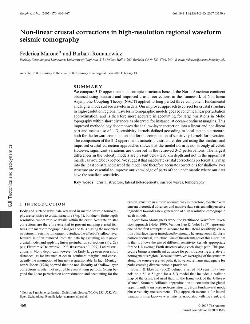
Geophys. J. Int. (2007) 170, 460–467 doi: 10.1111/j.1365-246X.2007.03399.xG

JITec

toni

csan

dge

ody

nam

ics

Non-linear crustal corrections in high-resolution regional waveformseismic tomography

Federica Marone∗ and Barbara RomanowiczBerkeley Seismological Laboratory, University of California, 215 McCone Hall #4760, Berkeley CA 94720-4760, USA. E-mail: [email protected]

Accepted 2007 February 9. Received 2007 February 9; in original form 2006 February 13

S U M M A R YWe compare 3-D upper mantle anisotropic structures beneath the North American continentobtained using standard and improved crustal corrections in the framework of Non-linearAsymptotic Coupling Theory (NACT) applied to long period three component fundamentaland higher mode surface waveform data. Our improved approach to correct for crustal structurein high-resolution regional waveform tomographic models goes beyond the linear perturbationapproximation, and is therefore more accurate in accounting for large variations in Mohotopography within short distances as observed, for instance, at ocean–continent margins. Thisimproved methodology decomposes the shallow-layer correction into a linear and non-linearpart and makes use of 1-D sensitivity kernels defined according to local tectonic structure,both for the forward computation and for the computation of sensitivity kernels for inversion.The comparison of the 3-D upper mantle anisotropic structures derived using the standard andimproved crustal correction approaches shows that the model norm is not strongly affected.However, significant variations are observed in the retrieved 3-D perturbations. The largestdifferences in the velocity models are present below 250 km depth and not in the uppermostmantle, as would be expected. We suggest that inaccurate crustal corrections preferentially mapinto the least constrained part of the model and therefore accurate corrections for shallow-layerstructure are essential to improve our knowledge of parts of the upper mantle where our datahave the smallest sensitivity.

Key words: crustal structure, lateral heterogeneity, surface waves, tomography.

1 I N T RO D U C T I O N

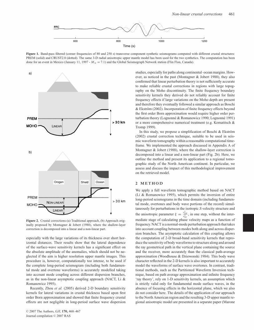
Body and surface wave data sets used in mantle seismic tomogra-

phy are sensitive to crustal structure (Fig. 1), but due to finite depth

resolution cannot resolve details within the crust. Accurate crustal

corrections are therefore essential to prevent mapping crustal fea-

tures into mantle tomographic images and thus biasing the modelled

structure. In seismic tomographic studies, the effect of shallow-layer

features is often removed from the data by assuming an a prioricrustal model and applying linear perturbation corrections (Fig. 2a)

(e.g. Ekstrom & Dziewonski 1998; Ritsema et al. 1999). Lateral vari-

ations in Moho depth can, however, be fairly large even over short

distances, as for instance at ocean–continent margins, and conse-

quently the assumption of linearity is questionable. In fact, Montag-

ner & Jobert (1988) showed that the non-linearity of shallow-layer

corrections is often not negligible even at long periods. Going be-

yond the linear perturbation approximation and accounting for the

∗Now at: Paul Scherrer Institut, Swiss Light Source/WLGA 135, 5232 Vil-

ligen, Switzerland. E-mail: [email protected].

crustal structure in a more accurate way is therefore, together with

current theoretical advances and massive data sets, an indispensable

ingredient towards a new generation of high resolution-tomographic

earth models.

Apart from Montagner’s work, the Partitioned Waveform Inver-

sion approach (Nolet 1990; Van der Lee & Nolet 1997) represents

one of the first attempts to account for the lateral sensitivity varia-

tion of surface waves introduced by strongly heterogeneous Earth (in

particular crustal) structure. One of the advantages of this algorithm

is that it allows the use of different sensitivity kernels appropriate

for the 1-D average Earth structure along each single path. This pro-

cedure brings a significant advance for paths traversing a relatively

homogeneous region. Because it involves averaging of the structure

along the source–receiver path, it, however, remains inadequate for

paths crossing diverse tectonic provinces.

Boschi & Ekstrom (2002) defined a set of 1-D sensitivity ker-

nels on a 5◦ × 5◦ grid for a 3-D model that includes a realistic

map of the crust, and used them in the framework of the Jeffreys-

Wentzel-Kramers-Brillouin approximation to constrain the global

upper mantle transverse isotropic structure from fundamental mode

phase velocity measurements. This approach accounts for lateral

variations in surface-wave sensitivity associated with the crust, and

460 C© 2007 The Authors

Journal compilation C© 2007 RAS

Non-linear crustal corrections 461

Figure 1. Band-pass filtered (corner frequencies of 80 and 250 s) transverse component synthetic seismograms computed with different crustal structures:

PREM (solid) and CRUST2.0 (dotted). The same 3-D radial anisotropic upper mantle model has been used for the two synthetics. The computation has been

done for an event in Mexico (January 11, 1997 - M w = 7.1) and the Global Seismograph Network station (Flin Flon, Canada).

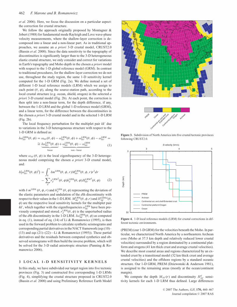
Linear

PREM

MOHO> 30 km

Linear

PREM

MOHO> 30 km

LINEAR

PREM

MOHO> 30 km

PREM

MOHO> 30 km

Orogen OceanShield

LINEAR

N -ON LINEAR

b)

a)

Figure 2. Crustal corrections-(a) Traditional approach, (b) Approach orig-

inally proposed by Montagner & Jobert (1988), where the shallow-layer

correction is decomposed into a linear and a non-linear part.

especially with the large variations of its thickness over short hor-

izontal distances. Their results show that the lateral dependence

of the surface-wave sensitivity kernels has a significant effect on

the absolute amplitude of the anomalies, which should not be ne-

glected if the aim is higher resolution upper mantle images. This

procedure is, however, computationally too intense, to be used if

the complete long-period seismogram (including both fundamen-

tal mode and overtone waveforms) is accurately modelled taking

into account mode coupling across different dispersion branches,

as in the non-linear asymptotic coupling approach (NACT, Li &

Romanowicz 1995).

Recently, Zhou et al. (2005) derived 2-D boundary sensitivity

kernels for lateral variations in crustal thickness based upon first

order Born approximation and showed that finite frequency crustal

effects are not negligible in long-period surface wave dispersion

studies, especially for paths along continental–ocean margins. How-

ever, as noticed in the past (Montagner & Jobert 1988), they also

confirmed that linear perturbation theory is not sufficiently accurate

to make reliable crustal corrections in regions with large topog-

raphy on the Moho discontinuity. The finite frequency boundary

sensitivity kernels they derived do not reliably account for finite

frequency effects if large variations on the Moho depth are present

and therefore they eventually followed a similar approach as Boschi

& Ekstrom (2002). Incorporation of finite frequency effects beyond

the first order Born approximation would require higher order per-

turbation theory (Lognonne & Romanowicz 1990; Lognonne 1991)

or a more comprehensive numerical treatment (e.g. Komatitsch &

Tromp 1999).

In this study, we propose a simplification of Boschi & Ekstrom

(2002) crustal correction technique, suitable to be used in seis-

mic waveform tomography within a reasonable computational time-

frame. We implemented the approach discussed in Appendix A of

Montagner & Jobert (1988), where the shallow-layer correction is

decomposed into a linear and a non-linear part (Fig. 2b). Here, we

outline the method and present its application to a regional tomo-

graphic study of the North American continent. In particular, we

assess and discuss the impact of this methodological improvement

on the retrieved model.

2 M E T H O D

We apply a full waveform tomographic method based on NACT

(Li & Romanowicz 1995), which permits the inversion of entire

long-period seismograms in the time domain (including fundamen-

tal mode, overtones and body wave portions of the record) simul-

taneously for perturbations in the isotropic S-velocity structure and

the anisotropic parameter ξ = v2SH

v2SV

, in one step, without the inter-

mediate stage of calculating phase velocity maps as a function of

frequency. NACT is a normal-mode perturbation approach that takes

into account coupling between modes both along and across disper-

sion branches. The asymptotic calculation of this coupling allows

the computation of 2-D broad-band sensitivity kernels that repro-

duce the sensitivity of body waveforms to structure along and around

the ray geometrical path in the vertical plane containing the source

and the receiver, more accurately than the classical path-average

approximation (Woodhouse & Dziewonski 1984). This body wave

character reflected in the 2-D kernels is also important to accurately

model the waveforms of surface wave overtones. In contrast, tradi-

tional methods, such as the Partitioned Waveform Inversion tech-

nique, based on path average approximation and infinite frequency

‘ray theory’, rely on 1-D sensitivity kernels, an assumption which

is strictly valid only for fundamental mode surface waves, in the

absence of focusing effects in the horizontal plane, which we also

do not consider here. The details of the application of our approach

to the North American region and the resulting 3-D upper mantle re-

gional anisotropic model are presented in a separate paper (Marone

C© 2007 The Authors, GJI, 170, 460–467


462 F. Marone and B. Romanowicz

et al. 2006). Here, we focus the discussion on a particular aspect:

the correction for crustal structure.

We follow the approach originally proposed by Montagner &

Jobert (1988) for fundamental mode Rayleigh and Love wave-phase

velocity measurements, where the shallow-layer correction is de-

composed into a linear and a non-linear part. As in traditional ap-

proaches, we assume an a priori 3-D crustal model, CRUST2.0

(Bassin et al. 2000). Since the data sensitivity to the topography of

discontinuities is significantly larger than to the 3-D heterogeneous

elastic crustal structure, we only consider and correct for variations

in Earth’s topography and Moho depth in the chosen a priori model

with respect to the 1-D global reference model (GRM). In contrast

to traditional procedures, for the shallow-layer correction we do not

use, throughout the study region, the same 1-D sensitivity kernel

computed for the 1-D GRM (Fig. 2a). We define instead a set of

different 1-D local reference models (LRM) which we assign to

each point (θ , φ), along the source-station path, according to the

local crustal structure (e.g. ocean, shield, orogen) in the selected apriori 3-D crustal model (Fig. 2b). At each point, the correction is

then split into a non-linear term, for the depth difference, if any,

between the 1-D LRM and the global 1-D reference model (GRM),

and a linear term, for the difference between the discontinuities in

the chosen a priori 3-D crustal model and in the selected 1-D LRM

(Fig. 2b).

The local frequency perturbation for the multiplet pair kk′ due

to variations in the 3-D heterogeneous structure with respect to the

1-D GRM is defined as:

δωGRMkk′ (θ, φ) = ωkk′(θ, φ) − ωLRM

kk′ (θ, φ) + ωLRMkk′ (θ, φ) − ωGRM

kk′ =∼= δωLRM

kk′ (θ, φ)︸︷︷︸linear

+ ωLRMkk′ (θ, φ) − ωGRM

kk′︸︷︷︸non−linear

(1)

where ωkk′ (θ , φ) is the local eigenfrequency of the 3-D heteroge-

neous model comprising the chosen a priori 3-D crustal model,

and:

δ(ωLRM

kk′ (θ, φ)2) =

∫ a

0

δmLRM(θ, φ, r )MLRMkk′ (θ, φ, r )r 2dr

−∑

d

rLRMd

2(θ, φ)hLRM

d (θ, φ)H LRMkk′

d(θ, φ) (2)

with δ mLRM (θ , φ, r ) and hLRMd (θ , φ) representing the deviation of

the elastic parameters and undulation of the dth discontinuity with

respect to their values in the 1-D LRM. MLRMkk′ (θ, φ,r ) and H LRM

kk′ d (θ ,

φ) are the respective local sensitivity kernels for the multiplet pair

kk′, which together with the eigenfrequencies ωLRMkk′ have been pre-

viously computed and stored. rLRMd (θ , φ) is the unperturbed radius

of the dth discontinuity in the 1-D LRM. δωGRMkk′ (θ , φ) as computed

in eq. (1), instead of eq. (14) of Li & Romanowicz (1995), is then

used in the forward problem to calculate synthetic seismograms and

corresponding partial derivatives in the NACT framework (eqs (10)–

(13) and eqs (21)–(22)—Li & Romanowicz (1995)). These partial

derivatives and the residuals between computed synthetics and ob-

served seismograms will then build the inverse problem, which will

be solved for the 3-D radial anisotropic structure (Panning & Ro-

manowicz 2006).

3 L O C A L 1 - D S E N S I T I V I T Y K E R N E L S

In this study, we have subdivided our target region into five tectonic

provinces (Fig. 3) and constructed five corresponding 1-D LRMs

(Fig. 4), simplifying the crustal structure proposed in CRUST2.0

(Bassin et al. 2000) and using Preliminary Reference Earth Model

PREM

Oce

an

Contin

enta

l arc

and

she

lf

Exten

ded

crus

t

Contin

enta

l platfo

rm

Oro

gen

Arche

an

Figure 3. Subdivision of North America into five crustal/tectonic provinces

following CRUST2.0.

0

50

De

pth

(km

)

3 4 5

S-velocity (km/s)

PREM

Archean

Continental arc and shelf/Extended crust

Continental platform/Orogen

Ocean

Figure 4. 1-D local reference models (LRM) for crustal corrections in dif-

ferent tectonic environments.

(PREM) (our 1-D GRM) for the velocities beneath the Moho. In par-

ticular, we characterized North America by a northeastern Archean

core (Moho at 37.5 km depth and relatively reduced lower crustal

velocities) surrounded by a region dominated by a continental plat-

form and orogens (41 km thick crust and average crustal velocities).

We describe most coastal areas and regions characterized by an ex-

tended crust by a transitional model (32 km thick crust and average

crustal velocities) and the offshore regions by a standard oceanic

structure. Our 1-D GRM, PREM (Dziewonski & Anderson 1981),

is assigned to the remaining areas (mostly at the ocean/continent

margin).

We compute the depth M kk′ (r ) and discontinuity H dkk′ sensi-

tivity kernels for each 1-D LRM thus defined. Large differences

C© 2007 The Authors, GJI, 170, 460–467



-150

-100

-100

-50

0

50

100

Mo

ho

kern

elp

ert

urb

atio

n%

Fundamental mode First overtone

-50

0

OceanOrogen

-30

-20

-10

0

Mo

ho

kern

elp

ert

urb

atio

n%

50 60 70 80 90 100 110

Period (s)

-30

-20

-10

0

10

20

30

50 60 70 80 90 100 110

Period (s)

Sp

he

roid

alm

od

es

To

roid

alm

od

es

Figure 5. Perturbation of spheroidal (top) and toroidal (bottom) mode sensitivity kernels for Moho depth H kk′ for 2 different 1-D models shown in Fig. 4

(ocean (circle), orogen (triangle)) with respect to PREM at three different periods, on the left for the fundamental mode, on the right for the first overtone.

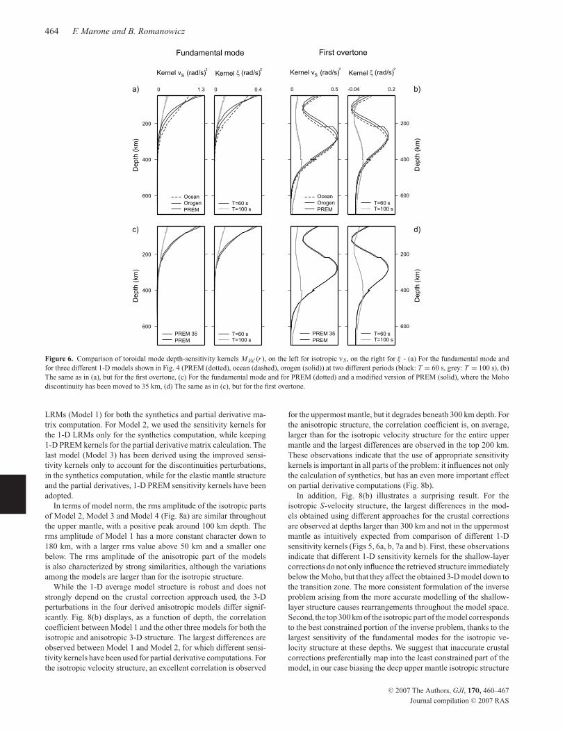
in the sensitivity kernels for Moho depth are observed both for

fundamental and higher modes (Fig. 5). As expected, variations

are larger at short periods (larger than 100 per cent for the first

spheroidal overtone), but even for a period of 100 s, differences reach

50 per cent both for fundamental and higher spheroidal modes. Dif-

ferent crustal structures, as present in the 1-D LRMs used, have a

large effect also on the depth-sensitivity kernels M kk′ (r ) (Figs 6a

and b, 7a and b), especially at short period (T = 60 s) both for

fundamental and higher toroidal modes. The observed variations

arise uniquely from the differences in the shallow structure, since

the velocities beneath the Moho are the same in all 1-D LRMs. As

expected, the largest effect of the crustal structure on the depth sen-

sitivity kernels is observed immediately beneath the Moho discon-

tinuity. Significant differences in M kk′ (r ) are, however, also present

well down into the upper mantle (200–400 km depth), in particu-

lar for toroidal modes. Similar conclusions can also be drawn from

the comparison (Figs 6c and d and 7c and d) of the depth sensitiv-

ity kernels for PREM and a modified version of PREM, where the

Moho discontinuity has been moved to 35 km depth, while the other

interfaces and the crustal and mantle velocities are not changed. Ac-

cordingly, although using the 1-D LRMs to correct for the shallow-

structure will mainly affect the uppermost mantle, we also expect

the deeper structure to be influenced. This comparison of depth

sensitivity kernels for 1-D models with different crustal structures

suggests that inaccurate correction for shallow-layer features can

map significantly deeper than just in the top upper mantle.

Our 3-D a priori crustal model for shallow-layer corrections con-

sists of two discontinuities: the Earth’s topography and Moho inter-

face. The Earth’s topography is modelled according to ETOPO-5

(National Geophysical Data Center 1988), the Moho interface ac-

cording to CRUST2.0 (Bassin et al. 2000). The accuracy of the

shallow-layer correction, in addition to the approach used to com-

pute it, obviously also depends on the accuracy of the chosen crustal

model. The locations at which crustal thickness has been deter-

mined with an accuracy of a few kilometers or less in refraction

and reflection experiments or in receiver function studies are un-

evenly distributed, with the highest density for continents in the

Northern Hemisphere. CRUST2.0 is currently the available global

crustal model based on the most up-to-date compilation of such

data, with the densest sampling in North America and Eurasia. For

the maximum resolution of this study (in the order of 500 km), the

accuracy of CRUST2.0 should be sufficient. However, one of the

requirements for future higher-resolution models will definitely be

improved knowledge of shorter wavelength crustal structures.

4 M O D E L A S S E S S M E N T

The aim of this paper is not the discussion of the obtained 3-D

anisotropic structure in terms of tectonic processes, which is the

topic of a separate publication (Marone et al. 2006). Here, we fo-

cus, instead, on a qualitative and quantitative comparison of the

models obtained using different approaches for the shallow-layer

corrections.

The 1-D LRMs are used in the forward problem, both for the

synthetics and partial derivative matrix computation. To evaluate

the significance of these more correct sensitivity kernels in the var-

ious parts of the problem, we computed the synthetics and partial

derivative in four different ways (Table 1), ran a similar inversion

in all cases and compared the derived 3-D anisotropic structure.

The two extreme models have been derived using either 1-D PREM

sensitivity kernels (Model 4) or the sensitivity kernels for the 1-D

C© 2007 The Authors, GJI, 170, 460–467



Figure 6. Comparison of toroidal mode depth-sensitivity kernels M kk′ (r ), on the left for isotropic vS , on the right for ξ - (a) For the fundamental mode and

for three different 1-D models shown in Fig. 4 (PREM (dotted), ocean (dashed), orogen (solid)) at two different periods (black: T = 60 s, grey: T = 100 s), (b)

The same as in (a), but for the first overtone, (c) For the fundamental mode and for PREM (dotted) and a modified version of PREM (solid), where the Moho

discontinuity has been moved to 35 km, (d) The same as in (c), but for the first overtone.

LRMs (Model 1) for both the synthetics and partial derivative ma-

trix computation. For Model 2, we used the sensitivity kernels for

the 1-D LRMs only for the synthetics computation, while keeping

1-D PREM kernels for the partial derivative matrix calculation. The

last model (Model 3) has been derived using the improved sensi-

tivity kernels only to account for the discontinuities perturbations,

in the synthetics computation, while for the elastic mantle structure

and the partial derivatives, 1-D PREM sensitivity kernels have been

adopted.

In terms of model norm, the rms amplitude of the isotropic parts

of Model 2, Model 3 and Model 4 (Fig. 8a) are similar throughout

the upper mantle, with a positive peak around 100 km depth. The

rms amplitude of Model 1 has a more constant character down to

180 km, with a larger rms value above 50 km and a smaller one

below. The rms amplitude of the anisotropic part of the models

is also characterized by strong similarities, although the variations

among the models are larger than for the isotropic structure.

While the 1-D average model structure is robust and does not

strongly depend on the crustal correction approach used, the 3-D

perturbations in the four derived anisotropic models differ signif-

icantly. Fig. 8(b) displays, as a function of depth, the correlation

coefficient between Model 1 and the other three models for both the

isotropic and anisotropic 3-D structure. The largest differences are

observed between Model 1 and Model 2, for which different sensi-

tivity kernels have been used for partial derivative computations. For

the isotropic velocity structure, an excellent correlation is observed

for the uppermost mantle, but it degrades beneath 300 km depth. For

the anisotropic structure, the correlation coefficient is, on average,

larger than for the isotropic velocity structure for the entire upper

mantle and the largest differences are observed in the top 200 km.

These observations indicate that the use of appropriate sensitivity

kernels is important in all parts of the problem: it influences not only

the calculation of synthetics, but has an even more important effect

on partial derivative computations (Fig. 8b).

In addition, Fig. 8(b) illustrates a surprising result. For the

isotropic S-velocity structure, the largest differences in the mod-

els obtained using different approaches for the crustal corrections

are observed at depths larger than 300 km and not in the uppermost

mantle as intuitively expected from comparison of different 1-D

sensitivity kernels (Figs 5, 6a, b, 7a and b). First, these observations

indicate that different 1-D sensitivity kernels for the shallow-layer

corrections do not only influence the retrieved structure immediately

below the Moho, but that they affect the obtained 3-D model down to

the transition zone. The more consistent formulation of the inverse

problem arising from the more accurate modelling of the shallow-

layer structure causes rearrangements throughout the model space.

Second, the top 300 km of the isotropic part of the model corresponds

to the best constrained portion of the inverse problem, thanks to the

largest sensitivity of the fundamental modes for the isotropic ve-

locity structure at these depths. We suggest that inaccurate crustal

corrections preferentially map into the least constrained part of the

model, in our case biasing the deep upper mantle isotropic structure

C© 2007 The Authors, GJI, 170, 460–467



Figure 7. Comparison of spheroidal mode depth sensitivity kernels M kk′ (r ), on the left for isotropic vS , on the right for ξ - (a) For the fundamental mode and

for three different 1-D models shown in Fig. 4 (PREM (dotted), ocean (dashed), orogen (solid)) at two different periods (black: T = 60 s, grey: T = 100 s), (b)

The same as in (a), but for the first overtone, (c) For the fundamental mode and for PREM (dotted) and a modified version of PREM (solid), where the Moho

discontinuity has been moved to 35 km, (d) The same as in (c), but for the first overtone.

Table 1. Type of 1-D sensitivity kernels used for synthetics and partial derivative matrices computation for different test models. Using

1-D sensitivity kernels for the global reference model (GRM), PREM in our case, implies utilizing the same eigenfunctions throughout

the study region. In contrast, using sensitivity kernels for local reference models (LRM) involves the use of different eigenfunctions in

different regions computed according to the local crustal structure.

Sensitivity kernels for: Synthetics Partial derivatives

Discontinuities Elastic mantle structure

Model 1 LRMs LRMs LRMs

Model 2 LRMs LRMs GRM

Model 3 LRMs GRM GRM

Model 4 GRM GRM GRM

and many of the anisotropic features. These results therefore imply

that accurate corrections for shallow-layer features are important to

improve our knowledge of parts of the upper mantle not optimally

constrained by the available data.

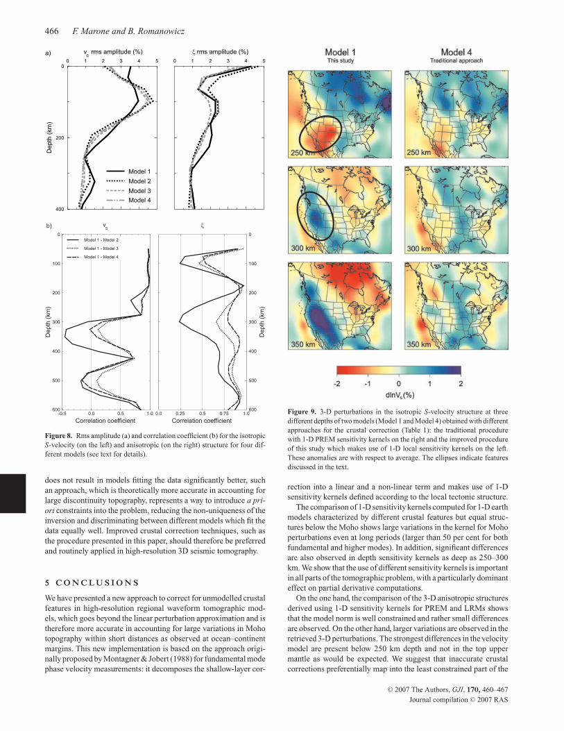
Fig. 9 visually compares the 3-D perturbations of the isotropic

structure in Model 1 and Model 4 at depths where the largest dis-

crepancies are observed (around 300 km, Fig. 8b). Both models

show positive anomalies beneath the northeastern part of the conti-

nent at 250 km depth as well as deeper fast mantle material in the

western United States. Despite similarities, these two models differ

in several details. Most remarkably Model 1 shows a much more

pronounced high velocity anomaly at 300–350 km depth beneath

the Western US than Model 4. This feature correlates well with the

expected position of the subducted part of the Juan de Fuca plate

in the North as suggested by higher resolution regional body wave

tomographic studies (e.g. Humphreys & Dueker 1994; Bostock &

VanDecar 1995) and could indicate the presence of remanents of the

Farallon plate in the South. In addition, the base of the North Amer-

ican craton is sharper in Model 1, where positive velocity anomalies

give way to a low-velocity region, possibly the asthenosphere, be-

neath 250–300 km depth, a feature not present in Model 4. Finally

although it is also visible in Model 1, the slab window in the Western

US (Dickinson & Snyder 1979) is more pronounced in Model 4.

Despite the observed differences, models derived using the tra-

ditional approach and more sophisticated crustal corrections fit the

used waveform data almost as well (Fig. 10, 67.0 per cent and 66.0

per cent variance reduction, respectively). In both cases, the largest

improvement in data fit is observed after the first iteration, while

for additional iterations, the curve quickly flattens. Although us-

ing 1-D sensitivity kernels tuned according to the tectonic structure

C© 2007 The Authors, GJI, 170, 460–467



Figure 8. Rms amplitude (a) and correlation coefficient (b) for the isotropic

S-velocity (on the left) and anisotropic (on the right) structure for four dif-

ferent models (see text for details).

does not result in models fitting the data significantly better, such

an approach, which is theoretically more accurate in accounting for

large discontinuity topography, represents a way to introduce a pri-ori constraints into the problem, reducing the non-uniqueness of the

inversion and discriminating between different models which fit the

data equally well. Improved crustal correction techniques, such as

the procedure presented in this paper, should therefore be preferred

and routinely applied in high-resolution 3D seismic tomography.

5 C O N C L U S I O N S

We have presented a new approach to correct for unmodelled crustal

features in high-resolution regional waveform tomographic mod-

els, which goes beyond the linear perturbation approximation and is

therefore more accurate in accounting for large variations in Moho

topography within short distances as observed at ocean–continent

margins. This new implementation is based on the approach origi-

nally proposed by Montagner & Jobert (1988) for fundamental mode

phase velocity measurements: it decomposes the shallow-layer cor-

Figure 9. 3-D perturbations in the isotropic S-velocity structure at three

different depths of two models (Model 1 and Model 4) obtained with different

approaches for the crustal correction (Table 1): the traditional procedure

with 1-D PREM sensitivity kernels on the right and the improved procedure

of this study which makes use of 1-D local sensitivity kernels on the left.

These anomalies are with respect to average. The ellipses indicate features

discussed in the text.

rection into a linear and a non-linear term and makes use of 1-D

sensitivity kernels defined according to the local tectonic structure.

The comparison of 1-D sensitivity kernels computed for 1-D earth

models characterized by different crustal features but equal struc-

tures below the Moho shows large variations in the kernel for Moho

perturbations even at long periods (larger than 50 per cent for both

fundamental and higher modes). In addition, significant differences

are also observed in depth sensitivity kernels as deep as 250–300

km. We show that the use of different sensitivity kernels is important

in all parts of the tomographic problem, with a particularly dominant

effect on partial derivative computations.

On the one hand, the comparison of the 3-D anisotropic structures

derived using 1-D sensitivity kernels for PREM and LRMs shows

that the model norm is well constrained and rather small differences

are observed. On the other hand, larger variations are observed in the

retrieved 3-D perturbations. The strongest differences in the velocity

model are present below 250 km depth and not in the top upper

mantle as would be expected. We suggest that inaccurate crustal

corrections preferentially map into the least constrained part of the

C© 2007 The Authors, GJI, 170, 460–467



0.50

0.52

0.54

0.56

0.58

0.60

0.62

0.64

0.66

0.68

0.70

Variance

reduct

ion

0 1 2 3 4

Iteration

Traditional approachThis study

Figure 10. Variance reduction as a function of number of iterations achieved

following the traditional approach with 1-D PREM sensitivity kernels (cir-

cle) and the improved procedure of this study which makes use of 1-D local

sensitivity kernels (triangle).

model and therefore conclude that accurate corrections for shallow-

layer features are important to improve our knowledge of parts of the

upper mantle where our data have the least sensitivity. For instance,

our 3-D anisotropic model derived with this improved approach

shows a high velocity anomaly at 300–350 km depth beneath the

Western US, possibly the signature of the subducted Juan de Fuca

and Farallon slabs, which is barely retrieved, if a standard crustal

correction approach is used.

A C K N O W L E D G M E N T S

We thank Mark Panning for extensive discussions during the im-

plementation phase of this study. This research was partially sup-

ported through a grant from the Stefano Franscini Foundation

(Switzerland) and NSF-EAR (Earthscope) grant #0345481. The

digital seismograms used in our work have been distributed by the

IRIS-DMC, the Geological Survey of Canada and the Northern Cal-

ifornia Earthquake Data Center (data contributed by the Berkeley

Seismological Laboratory, University of California, Berkeley). Con-

tribution number 06-01 of the Berkeley Seismological Laboratory,

University of California.

R E F E R E N C E S

Bassin, C., Laske, G. & Masters, G., 2000. The current limits of resolution for

surface wave tomography in North America, in EOS, Trans. Am. geophys.Un., Vol. 81, p. F897, Fall Meet. Suppl.

Boschi, L. & Ekstrom, G., 2002. New images of the Earth’s upper mantle

from measurements of surface wave phase velocity anomalies, J. geophys.Res., 107, 10.1029/2000JB000059.

Bostock, M. & VanDecar, J., 1995. Upper mantle structure of the Northern

Cascadia subduction zone, Can. J. Earth Sci., 32, 1–12.

Dickinson, W. & Snyder, W., 1979. Geometry of subducted slabs related to

San Andreas transform, J. Geol., 87, 609–627.

Dziewonski, A. & Anderson, D., 1981. Preliminary reference earth model,

Phys. Earth planet. Inter., 25, 297–356.

Ekstrom, G. & Dziewonski, A., 1998. The unique anisotropy of the Pacific

upper mantle, Nature, 394, 168–172.

Humphreys, E. & Dueker, K., 1994. Western U.S. upper mantle structure,

J. geophys. Res., 99, 9615–9634.

Komatitsch, D. & Tromp, J., 1999. Introduction to the spectral element

method for three-dimensional seismic wave propagation, Geophys. J. Int.,139, 806–822.

Li, X. & Romanowicz, B., 1995. Comparison of global waveform inversions

with and without considering cross branch coupling, Geophys. J. Int., 121,695–709.

Lognonne, P., 1991. Normal modes and seismograms of an anelastic rotating

Earth, J. geophys. Res., 96, 20309–20319.

Lognonne, P. & Romanowicz, B., 1990. Modelling of coupled normal

modes of the Earth: the spectral method, Geophys. J. Int., 102, 365–

395.

Marone, F., Gung, Y. & Romanowicz, B., 2006. 3-D radial anisotropic struc-

ture of the North American upper mantle from inversion of surface wave-

form data, Geophys. J. Int., in revision.

Montagner, J.-P. & Jobert, N., 1988. Vectorial tomography; II. Application

to the Indian Ocean, Geophys. J., 94, 309–344.

National Geophysical Data Center, 1988. ETOPO-5, bathymetry/topography

data, Data Announc. 88-MGG-02, Natl. Oceanic and Atmos. Admin., U.S.

Dep. of Commer., Washington, DC.

Nolet, G., 1990. Partitioned waveform inversion and 2-dimensional structure

under the network of autonomously recording seismographs, J. geophys.Res., 95, 8499–8512.

Panning, M. & Romanowicz, B., 2006. A three dimensional radially

anisotropic model of shear velocity in the whole mantle, Geophys. J. Int.,167, 361–379.

Ritsema, J., Van Heijst, H. & Woodhouse, J., 1999. Complex shear wave

velocity structure imaged beneath Africa and Iceland, Science, 286, 1925–

1928.

Van der Lee, S. & Nolet, G., 1997. Upper mantle S-velocity structure of

North America, J. geophys. Res., 102, 22 815–22 838.

Woodhouse, J. & Dziewonski, A., 1984. Mapping the upper mantle: three

dimensional modelling of earth structure by inversion of seismic wave-

forms, J. geophys. Res., 89, 5953–5986.

Zhou, Y., Dahlen, F., Nolet, G. & Laske, G., 2005. Finite-frequency ef-

fects in global surface-wave tomography, Geophys. J. Int., 163, 1087–

1111.

C© 2007 The Authors, GJI, 170, 460–467


Documents

Non-linear crustal corrections in high-resolution regional ...seismo.berkeley.edu/~barbara/REPRINTS/marone-gji07-crustal.pdf · Non-linear crustal corrections in high-resolution regional