Non-linear Prediction - Zentraler Informatikdiensthomepage.univie.ac.at/robert.kunst/non10_prean_lindner.pdf · Non-linear time series: pred. distributions usually not normal Furthermore:

MotivationExample and Theory IExample and Theory II

Concluding remarks

Non-linear Prediction

Nora Prean and Peter Lindner

18th January 2011

Nora Prean and Peter Lindner Non-linear Prediction


Concluding remarks

Contents

1 Motivation

2 Example and Theory ISimplest caseLeast squares m-step-ahead predictor

3 Example and Theory IIExample: Predictive distributionTheory again: Estimate predictive distributions

4 Concluding remarksNon-linear versus linear predictionLiteratureAppendix



Concluding remarks

Motivation

Basic idea of the presentation

Get a short introduction to non-linear prediction (Fan & YaoChapter 10)

Set-up: Why −→ Examples −→ Bits of the theory

Why forecasting? What is it for?

Who does not want to know the future?

Policy decisions depend on forecasts (e.g. future developmentof GDP)

How to become rich (Financial markets)

In the end, that is why we do time series analysis



Concluding remarks

Simplest caseLeast squares m-step-ahead predictor

Simple Quadratic Model to understand the graphs andsensitivity to initial values

Xt = 0.235Xt−1(16− Xt−1) + εt

whereεt ∼ U[−0.52, 0.52]

Now, we look at

m=2 and 3 step ahead predictor fm(•)their conditional variance function

and a comparison of the conditional variance.



Concluding remarks


m=2 step ahead predictor

Figure: m=2 step ahead predictor with different initial values

Predictive error depends on initial value

Can be seen from the deviation from the dots and the line

and the conditional variance

Legend

a Dots: Scatter plot Xt+2 against Xt

b Solid line: 2-step ahead predictor fm(•)c Impulses: Conditional variance σ2

m(•)



Concluding remarks



Figure: m=3 step ahead predictor with different initial values

Predictive error may be larger or smaller than for the m=2 step ahead predictor

Legend

a Dots: Scatter plot Xt+3 against Xt

b Solid line: 3-step ahead predictor fm(•)

c Impulses: Conditional variance σ2m(•)

Back



Concluding remarks


Conditional Variance

Figure: Conditional variance depending on initial values

In the ranges where the solid line is below the dotted line, the 3-step predictor is

more accurate than the 2-step predictor More

Legend

a Dotted line: Conditional variance of the 2-step-ahead predictorb Solid line: Conditional variance of the 3-step-ahead predictor



Concluding remarks


Least squares predictor

Observations from time series process X1, ...XT

Predict XT+m (m ≥ 1) based on last p observed values(XT ,XT−1, ...XT−p+1)τ ≡ XT

Predictor: fT ,m(XT ) = arg inf E{XT+m − f (XT )}2

compare OLS: β = arg min S(b) = (X ′X )−1X ′ywith S(b) =

∑ni=1(yi − x ′i b)2 = (y − Xb)′(y − Xb)

−→ fT ,m(x) = E (XT+m|XT = x)



Concluding remarks


Conditional variances given XT

Mean Square Predictive Error of fT ,m:

E{XT+m − fT ,m(XT )}2

= E [E{(XT+m − fT ,m(XT ))2|XT}]

= E{Var(XT+m|XT )}→ average of conditional variances of XT+m given XT

Note that for XT being a linear AR(p) conditional variance isconstant:

σ2T ,m(x) ≡ Var(XT+m|XT = x)

CONDITIONAL Mean Square Predictive Error:

E [{XT+m − fT ,m(x)}2|XT = x] = σ2T ,m(x) (1)



Concluding remarks


Decomposition of conditional mean square error

Decomposition: E [{XT+m − fT ,m(x)}2|XT = x + δ]

= σ2T ,m(x + δ) + {δτ fT ,m(x)}2 + o(||δ||2) (2)

In non-linear time series we might not neglect the error comingfrom the drift δ!For non-linear processes both types of errors may be amplifiedrapidly at some places in the state-space → hence it isimportant for predictions at which point we are!



Concluding remarks


Noise Amplification

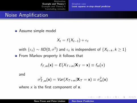
Assume simple model

Xt = f (Xt−1) + εt

with {εt} ∼ IID(0, σ2) and εt is independent of {Xt−k , k ≥ 1}From Markov property it follows that

fT ,m(x) = E (XT+m|XT = x) ≡ fm(x)

andσ2T ,m(x) = Var(XT+m|XT = x) ≡ σ2m(x)

where x is the first component of x.



Concluding remarks


For linear processes, e.g. an AR(1) process, the noise enteringat a fixed point in time decays exponentially as m increases.This noise contraction is not necessarily observed in non-linearprocesses.For Xt = f (Xt−1) + εt

σ2m(x) = Var(Xm|X0 = x) = µm(x)σ2 + O(ζ3)

with

µm(x) = 1 +m−1∑j=1

m−1∏k=j

f [f (k)(x)]

2

σ2m(x) varies with xµm(x) dictates noise amplification (for linear processes σ2

m(x) andµm(x) are constant).Values of µm are determined by those of the derivative f

If |f (.)| > 1 defines large state-space, µm(.) can be large even for

small m See Maybe Conclusion



Concluding remarks

Example: Predictive distributionTheory again: Estimate predictive distributions

Predictive Distribution: Different estimators

Nadaraya-Watson estimator (NW)

Local linear regression estimator (LL)

adjusted Nadaraya-Watson estimator (ANW)

Local logistic estimator (LG-2)

Compare them using mean absolute deviation error (MADE)

MADE =

∑i |Fe(yi |xi )− F (yi |xi )|I{0.001 ≤ F (yi |xi ) ≤ 0.999}∑

i I{0.001 ≤ F (yi |xi ) ≤ 0.999}



Concluding remarks


Example II: Model

Yt = 3.76Yt−1 − 0.235Y 2t−1 + 0.3εt

whereεt independent with common distribution U[−0.52, 0.52]

Look at conditional distribution function z = F (y |x) for m=2and 3

and a compare the predicted distribution using MADE.



Concluding remarks


Conditional Distribution Function for m = 2

Figure: CDF for m = 2

Legend

a X-Axis: past observed values

b Y-Axis: predicted values

c Vertical axis: Probability z = F (y|x)



Concluding remarks


Conditional Distribution Function for m = 3

Figure: CDF for m = 3

Legend

a X-Axis: past observed values

b Y-Axis: predicted values

c Vertical axis: Probability z = F (y|x)



Concluding remarks


Comparison of the Conditional Distribution Function

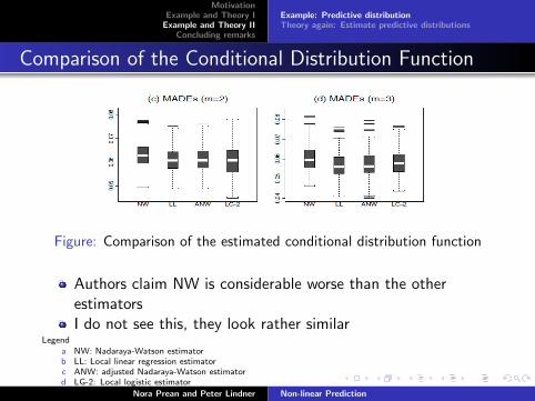
Figure: Comparison of the estimated conditional distribution function

Authors claim NW is considerable worse than the otherestimatorsI do not see this, they look rather similar

Legenda NW: Nadaraya-Watson estimatorb LL: Local linear regression estimatorc ANW: adjusted Nadaraya-Watson estimatord LG-2: Local logistic estimator



Concluding remarks


Estimate predictive distributions

Generally: forecast a predictive interval/predictive set

”All information on the future is [...]contained in a predictivedistribution function, which is in fact a conditionaldistribution of a future variable given the present state.”(F&Y, p. 454)

Linear time series: predictive distributions are normal (hence,simply estimate means and variances)

Non-linear time series: pred. distributions usually not normalFurthermore: even if process is generated by parametricnon-linear model the multiple-step-ahead predictivedistributions are of unknown form and may only be estimatedin a non-parametric manner



Concluding remarks


Local linear regression estimator (LL)

Assume: data from str. stat. stochastic process {(Xt ,Yt)}where Xt = (Xt , ...,Xt−p+1)τ typically denotes a vector oflagged values of Yt = Xt+m for some m ≥ 1

Estimate conditional distribution function

F (y |x) ≡ P(Yt ≤ y |Xt = x)

Rewrite I (Yt ≤ y) = Zt , then

F (y |x) = E (Zt |Xt = x)

Hence, estimation problem can be viewed as regressionof Zt on Xt by local linear technique (see F&Y 8.2)

−→ yields our Local Linear regression estimator (LL)

Problem: estimator F (y |x) is not necessarily a CDF



Concluding remarks


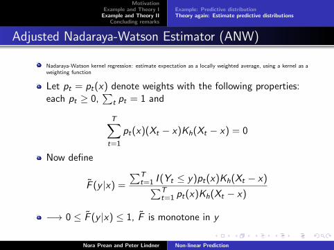
Adjusted Nadaraya-Watson Estimator (ANW)

Nadaraya-Watson kernel regression: estimate expectation as a locally weighted average, using a kernel as aweighting function

Let pt = pt(x) denote weights with the following properties:each pt ≥ 0,

∑t pt = 1 and

T∑t=1

pt(x)(Xt − x)Kh(Xt − x) = 0

Now define

F (y |x) =

∑Tt=1 I (Yt ≤ y)pt(x)Kh(Xt − x)∑T

t=1 pt(x)Kh(Xt − x)

−→ 0 ≤ F (y |x) ≤ 1, F is monotone in y



Concluding remarks

Non-linear versus linear predictionLiteratureAppendix

Conclusions

Linear prediction methods still dominant in time seriesforecasting

Linear prediction does well, whenever time series is covariancestationary (finite second moments)

Nevertheless, the best linear predictor is not the least squarespredictor in general and hence not the best estimator

Life (real-life generating processes) is not always linear!

Initial value sensitivity



Concluding remarks


Literature

Nonlinear Time Searies: Nonparametric and Parametric Methods

Fan, Jianqing and Yoa, Qiwei, Springer Series in Statistics (2003);especially Chapter 10

Quantifying the inference of initial values on nonlinear prediction

Yao, Q. and Tong, H. (1994); Journal of the Royal StatisticalSociety, Series B, 56, 701-725.



Concluding remarks


THANKS FOR YOUR ATTENTION



Concluding remarks


Modified Simple Quadratic Model: Point Prediction

Xit = 0.23Xt−1(16− Xt−1) + 0.4εt

whereεt ∼ iidN[0, 1]

on the interval [−12, 12].

draw a sample of 1,200 data points

σ21(x) = 0.16 due to iid normality, thus m=1 is not reportedin the book

look at m=2, 3, and 4 step ahead predictor for sample point1001 to 1200 and compare them to actual values



Concluding remarks



Figure: m=2 step ahead predictor with bandwidth h = 0.25

Legend

a Diamonds: Predicted values

b Solid line: Estimated conditional variance σ2m(•)

c Impulses: Absolute errors



Concluding remarks




Legend






Concluding remarks




Legend




Back


Documents

Non-linear Prediction - Zentraler Informatikdiensthomepage.univie.ac.at/robert.kunst/non10_prean_lindner.pdf · Non-linear time series: pred. distributions usually not normal Furthermore: