Embed Size (px)
Citation preview
Econometrics Journal (2006), volume 9, pp. 511–540.doi: 10.1111/j.1368-423X.2006.00196.x
Non-parametric regression for binary dependent variables
MARKUS FROLICH
Department of Economics, University of St.Gallen, Bodanstrasse 8, SIAW, 9000 St. Gallen,Switzerland;
E-mail: [email protected]
Received: August 2002
Summary Finite-sample properties of non-parametric regression for binary dependentvariables are analyzed. Non parametric regression is generally considered as highly variablein small samples when the number of regressors is large. In binary choice models,however, it may be more reliable since its variance is bounded. The precision in estimatingconditional means as well as marginal effects is investigated in settings with many explanatoryvariables (14 regressors) and small sample sizes (250 or 500 observations). The Klein–Spadyestimator, Nadaraya–Watson regression and local linear regression often perform poorly in thesimulations. Local likelihood logit regression, on the other hand, is 25 to 55% more precisethan parametric regression in the Monte Carlo simulations. In an application to female laboursupply, local logit finds heterogeneity in the effects of children on employment that is notdetected by parametric or semiparametric estimation. (The semiparametric estimator actuallyleads to rather similar results as the parametric estimator.)
Keywords: Binary choice, Local parametric regression, Local model, Heterogeneousresponse, Heterogeneous treatment effect.
1. INTRODUCTION
In this paper, non-parametric regression for binary dependent variables in finite-samples isanalyzed. Binary choice models are of great importance in many economic applications, butnon-parametric regression has received relatively little attention so far. Let Y ∈ {0, 1} be a binaryoutcome variable and X a vector of covariates. Often we are interested in estimating the conditionalmean E[Y |X = x] and/or the marginal effects E[Y |X = x + �x] − E[Y |X = x].
Usually, parametric regression models such as maximum likelihood probit or logit are used,which however entail restrictive functional form assumptions. Semiparametric binary choiceestimators, such as the Klein and Spady (1993) estimator, relax these restrictions, but still implyassumptions that can be restrictive in empirical applications. The single index restriction, inparticular, effectively reduces the heterogeneity in the X characteristics to a single dimension. Withthe recent emergence of the treatment evaluation literature, however, heterogeneity of treatmenteffects often has become of interest in itself (see e.g. Heckman et al. 1997). For example, in theanalysis of the effects of children on female labour supply, the marginal effect of an additionalchild on the employment probability is likely to depend also on other characteristics. Whereas the
C© Royal Economic Society 2006. Published by Blackwell Publishing Ltd, 9600 Garsington Road, Oxford OX4 2DQ, UK and 350 MainStreet, Malden, MA, 02148, USA.
512 Markus Frolich
effect is usually negative for most women, it might also be positive for some because of increasedfinancial needs (e.g. housing) due to a larger family (particularly if the children are older). Ifwomen react differently on the number of children, policy instruments such as subsidized childcare, all-day schooling or tax incentives should be targeted more precisely; particularly if thesubpopulation of women who increase their labour supply in response to an additional childcan be identified and distinguished from those women who reduce their labour supply. Suchheterogeneity in the effects on the employment probability can be of substantial interest in manyapplications, and the estimation model should be sufficiently flexible to not restrict such kind ofeffect heterogeneity from the outset.1
Fully non-parametric regression allows for this flexibility, but is rarely used for the estimationof binary choice applications. A reason might be that the prototypical application of non-parametric regression, which is local linear regression on a low dimensional vector of covariates,is not so well suited for binary choice models. On the one hand, linear probability models oftenperform poorly in binary choice settings compared to non-linear models such as probit or logit (seee.g. Hyslop 1999). Local non-linear estimation, such as local likelihood logit, might thereforebe better suited for binary dependent variables than local linear regression. In addition, locallikelihood logit encompasses the parametric logit model for a bandwidth value of infinity.
On the other hand, in many empirical applications one often wants to include a rather largenumber of covariates.2 Nonparametric regression in higher dimensions, however, is regardedas highly unreliable due to not only the curse of dimensionality but also small sample varianceproblems. For example, Seifert and Gasser (1996) show that local linear regression has a very highvariance when the data are sparse or clustered.3 Although the curse of dimensionality does notdisappear with binary dependent variables, the finite-sample variance problems are amelioratedbecause of the boundedness of Y .
The purpose of this paper is to examine the finite-sample performance of local likelihood logitfor binary dependent variables with many regressors (relative to the number of observations), ofwhich some are continuous and some are discrete. Local likelihood logit is compared to parametriclogit regression, the Klein and Spady (1993) estimator and to local linear and Nadaraya–Watsonregression. Whereas Klein–Spady, Nadaraya–Watson and local linear regression perform ratherpoorly in the Monte Carlo simulations, local logit is often more precise than parametric logit. Evenwhen the logit model is globally true, local likelihood logit does not perform much worse thanparametric logit, because in these cases larger bandwidth values are chosen by the cross-validationbandwidth selector. Precision gains are largest for the estimation of the conditional expectationsP(Y = 1|X ), and somewhat smaller for the estimation of marginal effects.
Local likelihood logit is then applied to analyze the dependence of Portuguese women’s laboursupply on the number of children. While the parametric logit and the semiparametric Klein–Spady estimator lead to rather similar estimates, local likelihood logit unveils heterogeneity inthe marginal effects of children that is unnoticed by the parametric logit estimator. Although theKlein–Spady estimator also detects some heterogeneity in the effects, it seems to be an artefact
1 Further examples where effect heterogeneity is of interest include the returns to schooling or the effects of trainingprogrammes, which can be used for designing optimal treatment rules, (see Manski 2000, 2004).
2 For identifying causal effects, usually all covariates that affect the outcome variable and the treatment variable haveto be included, which are often rather many, (see Rubin 1974; Holland 1986 Pearl 2000).
3 Because the denominator of the estimator can be arbitrarily close to zero. This happens often even at bandwidthvalues that are only slightly below the optimal value. Due to this, the unconditional finite-sample variance of local linearregression is infinite and the conditional variance is unbounded.
C© Royal Economic Society 2006
Non-parametric regression for binary dependent variables 513
of its larger variability.4 In Section 2, the local logit estimator is introduced. Section 3 providesthe simulation study. Section 4 analyzes female labour supply, and Section 5 concludes.
2. NONPARAMETRIC REGRESSION FOR BINARY DEPENDENT VARIABLES
Let Y ∈ {0, 1} be a binary outcome variable and X ∈ �Q+1 a vector of covariates, wherefor convenience of notation it is supposed that the last element of X is a constant. We areinterested in estimating the conditional mean E[Y |X = x] and the marginal effects E[Y |X =x + �x] − E[Y |X = x] for particular changes �x in the covariates. For continuous regressorsthe marginal effect is often defined as ∂ E[Y |X = x]/∂x q .5 The standard approach proceeds byspecifying a parametric model, for example, a probit or logit model, estimating the coefficients bymaximum likelihood and computing the conditional means and marginal effects. The disadvantageof parametric estimation is its reliance on functional form assumptions, which lead to inconsistentestimates if the model is not correctly specified.
Several semiparametric estimators have been suggested to relax these assumptions. A singleindex restriction is often invoked which assumes that the conditional mean can be specified asE[Y |X = x] = m(x ′θ ) with m an unknown function and θ an unknown coefficient vector. Anumber of
√n consistent estimators of θ have been developed, including iterative methods such
as Han (1987), Ichimura (1993), Klein and Spady (1993) and Sherman (1993) and non-iterativemethods such as the average derivative estimators of Hardle and Stoker (1989), Powell et al.(1989), Stoker (1991) and Horowitz and Hardle (1996). Although θ can often be estimated at√
n-rate, the function m(x′θ ) is non-parametric, and estimation of E[Y|X] and marginal effectswill be at a lower rate. The single index specification permits estimation at the univariate rate andthereby avoids the curse of dimensionality.
Although less restrictive than the parametric models, the single index specification still impliesthat all individuals can be aligned on a single dimension and restricts interactions between theregressors, which is less appealing for many econometric applications where heterogeneity inresponses (for example, treatment effects) is often considered as being important. For example,if Y is female labour supply and one covariate in X represents the number of children, the singleindex restriction imposes that the labour supply response of, for example, one versus zero childrenis identical for all women for whom the linear combination x′θ has the same value, even if theyhave very different characteristics. For these women, also the effect of five versus two children issupposed to be the same. In particular, the single-index restriction implies that any cross-effectsare independent of other characteristics. Hence, although the marginal effects ∂ E[Y |X = x]/∂x 1
can vary with x, the ratio of two marginal effects ∂ E[Y |X=x]/∂x1
∂ E[Y |X=x]/∂x2= θ1
θ2is not permitted to depend on
x. This is like a treatment–effect–homogeneity assumption and supposes that, for example, thelabour supply response to the number of children is identical to the labour supply response to achange in marginal tax rates (multiplied by the constant θ 1/θ 2) for every woman.
4 Gozalo and Linton (2000) apply least-squares local probit estimation to transport mode choice and find that parametricprobit regression misses some important regressor interaction effects, which are detected by local probit. This is also foundin the analysis of Portuguese female labour supply, where the estimated effects are examined instead of the coefficients,since the latter are of no direct interest. I also examine the performance of the Klein–Spady estimator, which also missesthe structure.
5 However, whereas E[Y |X = x + �x] − E[Y |X = x] is bounded, ∂ E[Y |X = x]/∂x q may not be.
C© Royal Economic Society 2006
514 Markus Frolich
Many of the other well-known semiparametric approaches also restrict interactions andresponse heterogeneity in that ∂ E[Y |X=x]/∂x1
∂ E[Y |X=x]/∂x2is not permitted to depend on any other covariates
than x1 and x2. This includes the generalized additive model (GAM), the partial linear model andthe generalized partial linear model.6,7
Nonparametric regression is more flexible. Although it is subject to the curse of dimensionalityand does not achieve
√n convergence, it may still perform well in finite samples.8 Local
polynomial regression is the most popular class of estimators, (see e.g. Fan and Gijbels 1996).Apart from Nadaraya–Watson (=local constant) regression, however, local polynomial regressionis not particularly suited for binary choice models as it does not incorporate the restriction thatE[Y |X ] ∈ [0, 1]. An immediate solution is to cap the estimates at 0 and at 1, which howevermakes the objective function non-differentiable and also implies that estimated marginal effectsmay be exactly zero at many x values.
Instead of local polynomials, other local models may be more appropriate. Let g(x , θ x ) bea known function with unknown coefficient vector θ x . The conditional mean function can bemodelled locally as
E[Y |X = x] = g(x, θx ). (1)
In contrast to the parametric and semiparametric models, the coefficient vector θ x is allowed tovary arbitrarily with x. Local parametric modelling includes Nadaraya–Watson (local constant)kernel regression with g(x , θ x ) = θ x and local linear regression with g(x , θ x ) = x ′θ x . For binarychoice models, the logit specification
E[Y |X = x].= 1
1 + e−x ′θx(2)
6 The generalized additive model (GAM) assumes that m(x) with dim(x) = K can be written as a sum of unknownnon-parametric functions of each component of x with a known link function G, e.g. the logit link,
G (E[Y |X = x]) = α + m1(x1) + m2(x2) + · · · + mK (xK ),
where the functions mk are unknown, (see Hastie and Tibshirani 1990). The partial linear model separates the componentsof x into two sets x S1 and x S2 and assumes that x S1 enters linearly whereas x S2 can enter non-parametrically through anunknown function m:
E[Y |X = x] = xS1 β + m(xS2 )
(see e.g. Robinson 1998). The generalized partial linear model extends this model with a known link function
G (E[Y |X = x]) = xS1 β + m(xS2 ).
In the last two models, usually the set x S2 contains only one regressor, which thus eliminates response heterogeneity. Ifx S2 contains several regressors often a generalized partial linear index model is used:
G (E[Y |X = x]) = xS1 β + m(x ′S2
θ ).
(see e.g. Pagan and Ullah 1999; Hardle et al. 2004, Fan and Gijbels 1996).7 More flexible are semiparametric models with multiple indices: E[Y |X = x] = α + ∑q
l=1ml (x ′θl ), which includesprojection pursuit (Friedman and Stuetzle 1981) and neural networks (White 1989; Kuan and White 1994).
8 In addition, the non-parametric regression estimates are often used as plug in estimates in some semiparametricestimation problem of the type discussed in Newey (1994) and Chen et al. (2003). Examples are partial means, averagetreatment effects or average derivative estimators, (see e.g. Blundell and Powell 2004; Frolich 2004, 2005, 2006; Hahn1998; Heckman et al. 1998; Hirano et al. 2003; Imbens 2004). Here,
√n-consistency can be achieved despite the low
precision in the non-parametric plug-in estimator, and the approaches with semiparametric structure mentioned abovebecome less attractive.
C© Royal Economic Society 2006
Non-parametric regression for binary dependent variables 515
is convenient, since it imposes the range restriction and is differentiable.9 If the logit form is closerto the true regression curve than a constant or linear specification, a non-parametric estimatorincorporating this local model will be less biased than kernel or local linear regression. Locallogit encompasses the global logit model (where θ x does not vary with x) and if the global logitmodel were indeed correct, local logit estimation would be unbiased.
Several approaches to estimate θx have been suggested. Local non-linear least-squaresregression Gozalo and Linton (2000) estimates θx from a sample of n i.i.d. observations {(Y i ,X i )}n
i=1 as
θx = arg minθx
n∑i=1
(Yi − g(Xi , θx ))2 K H (Xi − x), (3)
where K H (X i − x) is a kernel function and H a vector of bandwidth values.More general is local likelihood estimation which estimates θx as
θx = arg maxθx
n∑i=1
ln L (Yi , g(Xi , θx )) K H (Xi − x), (4)
where ln L(Y i , g(X i , θ x )) is the log-likelihood contribution of observation (Y i , X i ). For Hconverging to infinity, the local neighbourhood widens and the local estimator would converge tothe global parametric estimator.
Local likelihood estimation includes local least squares as a special case when the likelihoodfunction for normal errors is used. Local likelihood estimation has been introduced by Tibshiraniand Hastie (1987), and its properties have been analyzed in Fan et al. (1995), Fan and Gijbels(1996), Fan et al. (1998) and Eguchi et al. (2003), among others.10 Local likelihood estimationhas been used for density and hazard estimation,11 but only very rarely has it been applied toestimating regression functions for binary dependent variables. Tibshirani and Hastie (1987) andFan et al. (1995) consider exemplary biometric applications of local likelihood logit, but onlyfor one-dimensional X. Fan et al. (1998) present a brief simulation study and observed goodperformance of the local likelihood logit estimator, again only for one-dimensional X. For higher-dimensional X, Tibshirani and Hastie (1987) suggest non-parametric additive modelling for theregressors X, which, however, restricts interactions of the regressors.12 Only in the context oflocal least squares, an example for non-parametric regression with a binary dependent variableY and unrestricted interactions among the regressors X has been illustrated in Gozalo and Linton(2000).
9 Fan et al. (1995) and Fan et al. (1998) also consider higher, order expansions in the logit domain, e.g. with a quadraticterm: E[Y |X = x]
.= 11+e−αx −x ′βx −x ′γx x , where x does not contain a constant. A rather general result for local modelling
with local polynomials entering through a link function is that odd order polynomials lead to simpler asymptotic biasexpressions and with a bias of same order in the interior as in boundary regions, (see e.g. Fan et al. 1995; Carroll et al. 1998).This argument thus favours a linear or cubic expansion over a quadratic expansion. However, if x is higher dimensional,estimation with quadratic or even cubic terms could be difficult, since the number of coefficients proliferate quickly withdim(x) and local multicollinearity may occur more frequently.
10 See also Carroll et al. (1998) who proposed local estimating equations.11 See e.g. Copas (1995), Hjort and Jones (1996), Loader (1996), Staniswalis (1989), Fan and Gijbels (1996), Eguchi
and Copas (1998), Bebchuk and Betensky (2001) and Park et al. (2002).12 Blundell and Powell (2004) mentioned local likelihood probit estimation as one possible plug-in estimator for the
average structural function.
C© Royal Economic Society 2006
516 Markus Frolich
Compared to local least-squares regression, the local likelihood logit estimator has theadvantage of nesting the efficient estimator when the logit specification is true. In this case, theparametric maximum likelihood logit estimator is efficient, and for bandwidth values convergingto infinity the local likelihood logit estimator converges to the parametric logit estimator. Fornormal errors, i.e. when assuming that ε i is normally distributed in Y i = μ(X i ) + ε i , local non-linear least-squares regression and local likelihood estimation are identical. But the assumptionof normal errors is often not appropriate for binary dependent variables and is likely to lead toefficiency losses compared to a more sensible specification such as Y i = 1(μ(X i ) + ε i > 0),which leads to the local likelihood logit estimator for logistic ε i . In addition, the local likelihoodlogit estimator is globally concave and usually converged much faster to the solution than localnon-linear least squares.13
2.1. Local likelihood logit estimation
The local likelihood logit estimator is E[Y |X = x] = 11+e−x ′ θx
,14 where
θx = arg maxθx
n∑i=1
(Yi ln
(1
1 + e−Xi′θx
)+ (1 − Yi ) ln
(1
1 + eXi′θx
))K H (Xi − x). (5)
In many empirical applications, X may contain continuous as well as discrete variables.In principle, discrete variables could be accommodated by forming separate cells for eachcombination of the values of the discrete regressors and conducting separate regressions withineach cell. However, more precise estimates can be obtained by smoothing also over thediscrete regressors. Discrete regressors can easily be incorporated in the local model g(·). Forincluding discrete regressors also in the distance metric of the kernel function K (X i − x),Racine and Li (2004) suggested a hybrid product kernel that coalesces continuous and discreteregressors. They distinguish three types of regressors: continuous, discrete with natural ordering(number of children) and discrete without natural ordering (bus, train, car). Suppose that thevariables in X are arranged such that the first q1 regressors are continuous, the regressorsq 1 + 1, . . . , q 2 are discrete with natural ordering and the remaining Q − q 2 regressorsare discrete without natural ordering. Then the kernel weights K (X i − x) are computed
13 As an alternative to local models, it is often suggested to include a sufficient number of interaction terms in a globalparametric model. Although this might be a convenient approach in practice, some problems should be noted. If thenumber of covariates is large, the number of interaction terms can quickly exceed the number of observations. Even if allQ covariates are binary, 2Q different interaction terms can be formed. The estimates of such ‘saturated models’ can be veryimprecise because no smoothing over the covariates takes place, see e.g. Racine and Li (2004). In binary choice modelsestimated by maximum likelihood, several of the interaction terms might predict the outcome perfectly, thus leading tonumerical problems and undefined estimates. Although fully interacted models are often problematic in practice, a carefuldata-driven procedure to select from the many possible interaction terms might lead to similar results as a non-parametricapproach. This, however, is beyond the scope of this paper.
14 With g(x , θ x ) as the local model, the conditional mean is estimated as E[Y |X = x] = g(x, θx ). Marginal effects can beestimated either by estimating two conditional means E[Y |X = x + �x] − E[Y |X = x] = g(x + �x, θx+�x ) − g(x, θx )or from within the model as g(x + �x, θx ) − g(x, θx ).
C© Royal Economic Society 2006
Non-parametric regression for binary dependent variables 517
as
Kh,δ,λ(Xi − x) =q1∏
q=1
κ
(Xq,i − xq
h
) q2∏q=q1+1
δ|Xq,i −xq |Q∏
q=q2+1
λ1(Xq,i �=xq), (6)
where X q,i and x q denote the qth element of X i and x, respectively. 1(·) is the indicatorfunction. κ is a symmetric univariate kernel function. h, δ and λ are bandwidth parameterswith 0 ≤ δ, λ ≤ 1. This kernel function K h,δ,λ(X i − x) measures the distance between X i
and x through three components: The first term is the standard product kernel for continuousregressors. The second term measures the distance between the ordered discrete regressors andassigns geometrically declining weights. The third term measures the mismatch between theunordered discrete regressors. δ controls the amount of smoothing for the ordered and λ for theunordered discrete regressors. The larger δ and/or λ the more smoothing takes place with respectto the discrete regressors. If δ and λ are both 1, the discrete regressors would not affect the kernelweights and the non-parametric estimator would ‘smooth globally’ over the discrete regressors.On the other hand, if δ and λ are both zero, smoothing would proceed only within each of thecells defined by the discrete regressors but not between them.
Principally, instead of using only three bandwidth values h, δ, λ for all regressors, adifferent bandwidth could be employed for each regressor. This would substantially increase thecomputational burden for bandwidth selection and might lead to additional noise due to estimatingthese bandwidth parameters. Alternatively, groups of similar regressors could be formed, with eachgroup assigned a separate bandwidth parameter. Particularly if the ranges assumed by the ordereddiscrete variables vary considerably, those variables that take on many different values should beseparated from those with only few values. Moreover, the continuous regressors should be scaledto same mean and same standard deviation to adjust for different scopes and measurement scalesand to improve numerical stability.
2.2. Bandwidth choice
A large number of alternative bandwidth selection methods for non-parametric regression havebeen developed. For many plug-in methods, experience with their small sample behaviourfor higher-dimensional x is limited, though. In addition, with local parametric regression, theappropriate choice of the bandwidth parameters h, δ and λ depends also on how well the specifiedfunction g resembles the true conditional mean function. If the parametric hyperplane encompassesthe true conditional mean function, the optimal bandwidth values would be (h, δ, λ) = (∞, 1, 1),corresponding to (global) parametric regression. Otherwise the bandwidths should converge tozero with increasing sample size.15
15 Eguchi et al. (2003) analyze optimal bandwidth choice for local likelihood estimation under small h asymptoticsand large h asymptotics. If the local model is in an α-neighbourhood of the true conditional expectation function, theoptimal bandwidth tends to infinity as n increases to infinity. If the local model is far from the true conditional expectationfunction, the optimal bandwidth tends to zero as n increases. For some intermediate cases, the optimal bandwidth may beconstant. They argue that standard plug-in methods for bandwidth choice, which are based on small h asymptotics, arenot appropriate if it is a priori unknown how far the local model is from the true expectation function. On the other hand,they conjecture that cross-validation and bootstrap methods should be consistent in both situations, i.e. when the optimalbandwidth tends to infinity and when it tends to zero.
C© Royal Economic Society 2006
518 Markus Frolich
Bandwidth choice by cross-validation permits this ambiguity, i.e. if it is not a priori knownhow well the local parametric model fits the data. Cross-validation selects the bandwidths tominimize out-of-sample prediction error. For minimizing squared prediction error, the bandwidthsare chosen to minimize the least-squares criterion CV LS
CVLS =n∑
i=1
(Yi − g(Xi , θ−Xi |h,δ,λ))2, (7)
where θ−Xi |h,δ,λ is the leave-one-out coefficients estimate for the estimation of E[Y |X = X i ] thatis obtained from the data sample without observation i. The sum of squared errors indicates howwell the estimator is able to predict E[Y|X] for the sample distribution of X.
In the context of local likelihood estimation, Staniswalis (1989) suggested a different cross-validation criterion based on maximizing the leave-one-out fitted likelihood function
CVM L (h, λ) =n∑
i=1
Yi ln g(Xi , θ−Xi |h,δ,λ) + (1 − Yi ) ln(1 − g(Xi , θ−Xi |h,δ,λ)). (8)
2.3. Inference and confidence intervals
Fan and Gijbels (1996), Fan et al. (1998) and Carroll et al. (1998)16 discuss estimation of biasand variance of the local likelihood estimator. A consistent estimator of the local variance of θx
can be obtained as( ∑�i�i Xi X ′
i Ki
)−1( ∑(Yi − �i )
2 Xi X ′i K 2
i
)( ∑�i�i Xi X ′
i Ki
)−1
where �(u) = 11+e−u is the logit function and �i = �(X ′
i θx ) and �i = 1 − �i and �x = �(x ′θx )and �x = 1 − �x .17 For a small sample size, Carroll et al. (1998) and Galindo et al. (2001)propose a degrees of freedom correction.
The variance approximation for E[Y |X = x] can then be obtained by the delta methodas
Var(E [Y |X = x]
) ≈ �2x�
2x · x ′Var(θx )x .
Similarly, the variance of the marginal effects could be obtained by applying the delta methodto
∂ E [Y |X = x]
∂x= �(x ′θx )�(x ′θx ) θx
16 Carroll et al. (1998) analyzed local estimating equations (which contains local likelihood as a special case where thescore of the likelihood function gives the moment conditions) and derived consistent estimators for the variance, whichcorrespond to the following expressions.
17 Fan et al. (1998) and Carroll et al. (1998) propose modified versions of the variance estimator. Fan et al. (1998)replaces (Y i − �i )2 in the above expression by �x �x , whereas Carroll et al. (1998) replace (Y i − �i )2 by �i �i . Bothmodifications should lead to similar results if the smoothing window is small.
C© Royal Economic Society 2006

Non-parametric regression for binary dependent variables 519
to obtain
Var
(∂ E [Y |X = x]
∂x
)≈ �2
x�2x (I + (�x − �x )θx x ′)Var(θx )(I + (�x − �x )x θ ′
x ).
For obtaining confidence intervals also local bias has to be taken into account. Variousmethods to estimate the bias have been proposed, e.g. plug-in procedures using the asymptoticformulae for the bias and empirical procedures as suggested in Ruppert (1997) and Fanet al. (1998). The empirical approaches are usually based on higher order polynomials in thelogit link function, and there seems to be only limited experience with these methods forhigher dimensional X. With an estimate of the local bias, pointwise confidence intervals canbe constructed as described in Fan et al. (1998), exploiting the asymptotic normality of theestimate.
To avoid estimation of the local bias, undersmoothing through the choice of a smaller band-width value would reduce the magnitude of the bias at the expense of a larger variance. Withsufficient undersmoothing, the bias might become negligible compared to the variance such thatconfidence intervals can be based on estimated variance only. However, this undersmoothingclearly sacrifices precision. A more satisfying solution would be based on bootstrap confidenceintervals as derived in Galindo et al. (2001).
2.4. Local multicollinearity
Compared to conventional Nadaraya–Watson regression with unbounded kernel, a well-definedmaximizer of the local likelihood may not always exist or may be susceptible to numericalproblems when the smoothing window is small. First, it may happen that all observations in thelocal smoothing window are zeros or ones. Second, perfect prediction in the local smoothingwindow may result in coefficient estimates converging to infinity. Third, collinearity of theregressors in the local smoothing window can render the estimates undefined. These problemshave not been addressed in the literature so far, but could be quite important in finite samples.Obviously such problems should be of less concern when using a kernel with unbounded support,such as the Gaussian, compared to a compact kernel, such as the Epanechnikov. Nevertheless, evenwith the Gaussian kernel near-multicollinearity and perfect prediction can lead to very impreciseor undefined estimates.
The first problem could easily be solved by simply defining the estimate as one or zero ifall observations in the smoothing window are one or zero.18 In this case, marginal effects canno longer be computed directly from the local parametric model but require estimation of theconditional expectation function at x and x + �x .
To overcome the other two problems, there are essentially two approaches: locally increasingbandwidths or dropping regressors. Locally dropping regressors that cause collinearity reduces the
18 Fan et al. (1998) suggested to use only bandwidth values that are sufficiently large such that all local smoothingwindows contain zeros as well as ones. This, however, would not be the best solution if the true conditional expectationfunction E[Y |X = x] were indeed zero or one for some values of x, i.e. where the local logit model would be misspecified.Defining the estimate as zero or one is more in line with linear smoothers, which estimate the conditional expectationfunction as some weighted average of the observed Y in the smoothing window.
C© Royal Economic Society 2006
520 Markus Frolich
complexity of the local model,19 whereas increasing the bandwidth values reduces the localizationof the model. Different versions of the local likelihood logit estimator have been examined in thesimulations and led to largely similar results. Overall local likelihood logit with Gaussian kerneland increasing bandwidths in case of collinearity gave the best results in the Monte Carlo. (Moredetails are discussed in the supplementary appendix.)
3. FINITE SAMPLE PROPERTIES
In this section, the finite sample behaviour of local likelihood logit, local constant, local linearand Klein–Spady regression is analyzed for various simulation designs with 14 covariates(4 continuous, 10 binary) and samples of size 250 and 500, respectively. Hence, relative to thenumber of observations, the estimation problem can be considered as rather high-dimensional,since even the binary variables alone generate 1024 different cells. The out-of-sample predictionperformance is examined for the conditional mean E[Y|X] and for the marginal effects. Samples{(Y i , X i )}n
i=1 of size n are drawn as well as validation samples {X j}nj=1. From the sample {(Y i ,
X i )}ni=1 the conditional mean E[Y |X = X j ] is predicted at all locations X j and compared to the
true conditional mean E[Y |X = X j ].20 The marginal effects are estimated for all 14 variablesseparately. For a binary variable, the effect of a change from 0 to 1 is estimated. For a continuousvariable, the effect of an increase by 1 is estimated.21
The four continuous variables Xc1, Xc
2, Xc3, Xc
4 are drawn from different χ2 distributions,and the 10 binary variables Xb
1, . . . , Xb10 are Bernoulli distributed. Four different designs are
considered, which differ in the dependence structure among the covariates. In designs 1 and 2, thecontinuous variables are uncorrelated, while they are correlated in designs 3 and 4. The binaryvariables are uncorrelated in designs 1 and 3 but correlated in designs 2 and 4.
X-design 1: The continuous variables Xc1, Xc
2, Xc3, Xc
4 are independent and are distributed χ2 with1, 2, 3 and 4 degrees of freedom, respectively. The binary variables Xb
1, . . . , Xb10 are distributed
Bernoulli(p = 0.5). All variables are independent of each other.
X-design 2: The continuous variables are distributed independently as in X-design 1. The binaryvariables are dependent: Xb
1 ∼ Bernoulli(0.5) and Xbk ∼ Bernoulli(p = 0.3 + 0.4X b
k−1), whereX b
k−1 = 1k−1
∑k−1l=1 Xb
l is the mean of the realized values of the ‘preceding’ binary variables. Thus,
19 If all regressors except the constant are dropped, the estimator reduces to the Nadaraya–Watson estimator.20 The data sample {(Y i , X i )}n
i=1 and the validation sample {X j}nj=1 are drawn from the same population. The main
interest is often not in estimating the conditional mean and marginal effects at the locations of the data but at some otherlocation x0, provided x0 is in the support of X i . In the analysis of discrimination, we might be interested in predictingthe wages of women if they had the distribution of the human capital characteristics X that is observed among men. In atreatment evaluation context, we might be interested in predicting the earnings after participation in a training programmefor individuals who did not participate, by controlling for differences in the characteristics X. For such analyses we needthe support of X to be identical in both subpopulations, or more precisely, that the support of X in the validation sampleis a subset of the support of X in the data sample.
21 More precisely, the marginal effect is estimated as E[Y |X = X j ] − E[Y |X = X j ], where X j and X j differ fromX j only in the component corresponding to the variable for which the effect will be estimated. For the effect of a binaryvariable, the corresponding element is set to 1 in X j and to 0 in X j . For a continuous variable, X j equals X j and thecorresponding element in X j is increased by one.
C© Royal Economic Society 2006

Non-parametric regression for binary dependent variables 521
if all preceding variables are one, the probability that the next variable also takes the value one is0.7. The correlation among the binary variables lies between 0.1 and 0.4.
X-design 3: The binary variables are independent Bernoulli(0.5) variables as in X-design 1. Thecontinuous variables are positively correlated. Xc
1 is distributed χ2(1), Xc
2 is generated as Xc1 plus
an independent χ2(1), Xc
3 is generated as Xc2 plus an independent χ2
(1), and Xc4 is generated as Xc
3
plus an independent χ2(1). The implied correlation among the continuous variables lies between
0.5 and 0.9.
X-design 4: The continuous variables and the binary variables are dependent and generated as inX-design 3 and X-design 2, respectively.
The Y observations are generated according to one of the five Y-designs:
Y-design 1: Linear index model without interaction or higher-order terms
Y = 1
(−8 − Xc
1 + 2Xc2 − 3Xc
3 + 4Xc4 + 2
10∑k=1
Xbk (−1)k + noise > 0
).
Y-design 2: Linear index model with squared and interaction terms
Y = 1 if Y ∗ ≥ 0, where
Y ∗ = 8 − Xc21 + Xc2
2 − X23 + Xc2
4 + 3Xc1 − 5Xc
2 + 7Xc3 − 9Xc
4
+ 210∑j=1
Xbk (−1)k − Xc
1 Xb1 + Xc
2 Xb2 − Xc
3 Xb3 + Xc
4 Xb4 + noise
Y-design 3: Linear index model with interaction terms
Y = 1 if Y ∗ ≥ 0, where
Y ∗ = −8 − Xc1 + 2Xc
2 − 3Xc3 + 4Xc
4 + 210∑
k=1
Xbk (−1)k
− 3Xc1 Xb
1 Xb2 + 3Xc
2 Xb3 Xb
4 − 3Xc3 Xb
6 Xb7 + 3Xc
4 Xb8 Xb
9 + noise.
Y-design 4: Nonlinear model with lower and upper threshold
Y = 1 if 8 ≤ Y ∗ < 15, where
Y ∗ = 2√∣∣10 − Xc
1 − Xc2 + Xc
3 + Xc4
∣∣ − 0.3(Xc
1 + Xc2
) 4∑k=1
Xbk + 0.2
(Xc
3 + Xc4
) 10∑k=5
Xbk + noise
Y-design 5: Index model with two-regimes
Y = 1(Y ∗
1 ≥ 0)
if10∑
k=1
k Xbk is below its mean, and
Y = 1(Y ∗
2 ≥ 0)
otherwise, where
Y ∗1 = −4 − Xc
1 + Xc2 − Xc
3 + Xc4 − Xc
1 Xb1 + Xc
2 Xb2 − Xc
3 Xb3 + Xc
4 Xb4 + noise
Y ∗2 = − 4 + (−Xc
1 + Xc2 − Xc
3 + Xc4
)2 + 4(−Xc
1 Xb1 + Xc
2 Xb2 − Xc
3 Xb3 + Xc
4 Xb4
) + noise.
C© Royal Economic Society 2006
522 Markus Frolich
The first three Y-designs correspond to the latent index threshold passing model familiarfrom utility maximization theory: An individual chooses a certain option (purchasing a good,participating in the labour force) if her idiosyncratic latent utility exceeds a certain threshold(opportunity cost, reservation wage). In Y-design 1, the latent index is a linear combination of theregressors, as it is, for instance, modelled in a logit, probit or single-index model. In Y-design 2,square and interaction terms enter the latent index. Interaction terms with the binary regressorsare also included in Y-design 3. Y-design 4 represents a situation where a certain option is onlychosen if a latent index is neither too large nor too small. As an example, consider the relationshipbetween wages and the decision to work overtime. Overtime work will be attractive neither at verylow wages nor at very high wages due to the income (wealth) effect. Y-design 5 models differentbehavioural rules for two different subpopulations. According to their binary regressors, eachindividual belongs either to subpopulation one or to subpopulation two, and each subpopulationfaces a different outcome relationship. Such segregation might for instance be generated byadministrative regimes which induce different incentives among eligible and non-eligible groups,for example, affirmative action programmes, preferential tax treatments, exemptions from socialsecurity or pension contributions, etc.
Four different designs for the noise are considered: In the first variant, noise is drawn froma logistic distribution, a symmetric distribution with relatively little mass in the tails. Thisimplies that for Y-design 1 and logistic noise, the global logit model is correctly specifiedand the parametric logit estimator, which is used as the benchmark estimator, is consistent andefficient. In the second variant, referred to as heteroskedastic noise, the noise is drawn from
a t2 distribution and multiplied by 0.14√∑
Xck
∑Xb
k . This leads to a heteroskedastic error
with substantial probability mass in the tails.22 In the third variant, called bimodal, the noiseis drawn from a mixture of two normals N(2, 1) and N(−2, 1) leading to a symmetric bimodaldistribution. In the fourth variant, called asymmetric, the noise is drawn from the asymmetricχ2
(3) distribution. These four variants thus capture various features of the noise distribution.23
Except for the logistic noise in Y-design 1, the global parametric logit estimator is alwaysmisspecified.
3.1. Implementation of the estimators
All estimators use as regressors Xc1, . . . , Xc
4, Xb1, . . . , Xb
10 and a constant, but no interaction orhigher-order terms. The benchmark parametric logit is estimated by maximum likelihood.24
The semiparametric Klein–Spady estimator is implemented as in Gerfin (1996) with m(·)estimated by one-dimensional kernel regression and the bandwidth selected by generalized cross-validation. To be more specific, for a given bandwidth value h, the Klein–Spady estimatormaximizes the quasi-log-Likelihood function:
βh = arg maxβ
Q(β, h) =∑
i
Yi ln mi + (1 − Yi ) ln(1 − mi )
22 The variance of the t2 distribution is infinite.23 The mean of Y depends on the Y-design, X-design and the noise and varies between 0.43 and 0.56.24 If the parametric logit did not converge, e.g. collinearity or perfect prediction, a new sample is drawn.
C© Royal Economic Society 2006
Non-parametric regression for binary dependent variables 523
where
mi =∑
l Ylφ(
X ′lβ−X ′
i β
h·std(X ′β)
)∑
lφ(
X ′lβ−X ′
i β
h·std(X ′β)
)where std(X′β) is the standard deviation of X′β in the sample. For a given bandwidth value h, theestimates βh are obtained by Newton–Raphson iteration (with step size 0.2). Since the coefficientsβ are identified only up to scale, the first coefficient is normalized as one. The bandwidth is chosenthat minimizes the generalized cross-validation criterion
GCV (h) =∑
i (Yi − mi )2(∑i (1 − ξi )
)2
where
ξi = φ(0)∑lφ
(X ′
l βh−X ′i βh
h·std(X ′βh )
)is the kernel weight accorded to observation i in the estimation of mi . The GCV(h) is computed for30 different values of h ∈ {0.02, 0.04, . . . , 0.60} and the bandwidth corresponding to the minimumis chosen. With this estimated bandwidth h, the coefficients βh are estimated and estimates of theconditional mean at a value x are obtained as
E[Y |X = x] =∑
l Ylφ(
X ′l βh−x ′βh
h·std(X ′βh )
)∑
l φ(
X ′l βh−x ′βh
h·std(X ′βh )
) .
For the non-parametric Nadaraya–Watson, local linear and local logit estimators, thebandwidths are chosen either according to the least-squares criterion CV LS (7) or accordingto the likelihood criterion CV ML (8).25 The kernel weights K (X i − x) for given bandwidth valuesh, λ are computed in all estimators as
Kh,λ(Xi − x) =10∏
k=1
λ1(Xbk,i �=xb
k )4∏
k=1
κ
(Xc
k,i − xck
h
), (9)
where κ is either the Epanechnikov kernel κ(u) = 34 (1 − u2)1[−1,1](u) or the Gaussian kernel.
For local linear and local logit regression, the 14 regressors (plus a constant) enter not only inthe kernel function K (X i − x) but also in the local specification g(x , θ x ). To improve numericalaccuracy and to ensure that all continuous regressors are of similar magnitude, the continuousvariables are scaled to the same standard deviation prior to estimation. The estimated marginaleffects refer to the unscaled variables, though.
Local linear regression specifies the conditional expectation function locally as
E[Y |X = x].= x ′θx , (10)
25 From a grid of 20 × 20 gridpoints: (h, λ) ∈ {1, 1.2, . . . , 1.218, ∞} × {0.05, 0.10, 0.15, . . . , 1} for n = 250 and (h,λ) ∈ {1.2−6, 1.2−5, . . . , 1.212, ∞} × {0.05, 0.10, 0.15, . . . , 1} for n = 500.
C© Royal Economic Society 2006
524 Markus Frolich
where a constant is included among the regressors x. For given bandwidth values E[Y |X = x] isestimated by the first element of the weighted least-squares estimate θx , with
θx = (X′
x Wx Xx)−1
X′x Wx Yx ,
Xx =
⎛⎜⎜⎝1
(Xc
1,1 − xc1
) · · · (Xb
10,1 − xb10
)...
.... . .
...
1(Xc
1,n − xc1
) · · · (Xb
10,n − xb10
)⎞⎟⎟⎠ and Yx =
⎛⎜⎜⎝Y1
...
Yn
⎞⎟⎟⎠ and Wx = diag (K H (Xi − x))
(11)
(see Fan and Gijbels 1996; Ruppert and Wand 1994; Seifert and Gasser 1996). Since the locallinear estimates may lie outside the interval [0, 1], they are capped at zero and at one.
The local constant (Nadaraya Watson) estimator is a special case of local linear regressionwith all slope coefficients in (10) constrained to zero:
E[Y |X = x] =∑
Yi K H (Xi − x)∑K H (Xi − x)
.
3.2. Simulation results
The out-of-sample prediction performance for the conditional mean E[Y}X] and for the marginaleffects is assessed by their simulated mean absolute error (MAE), median absolute error (MdAE),mean squared error (MSE) and median squared error (MdSE). For each of the 80 differentdesigns,26 data samples and validation samples are drawn repeatedly27 from the same population,and for all observations of the validation sample the conditional means and marginal effects areestimated on the basis of the observations in the data sample, as described above. Since the MonteCarlo study comprehends a large number of different designs and variants of the estimators, onlythe most salient results are summarized in the following. A supplementary appendix, availablefrom the author’s webpage, contains all the detailed simulation results for all 80 designs.
The performance is measured relative to the benchmark parametric logit estimator, and allresults will be given in percent.28 Among these four performance measures, generally the relativeperformance of local logit is worst with respect to MSE and best with respect to MdSE. The relativeperformance with respect to the other two measures is usually between these two. Therefore, inthe following, only the results for the MSE and the MdSE are given. (The results for the meanand median absolute error can be found in the supplementary appendix.)
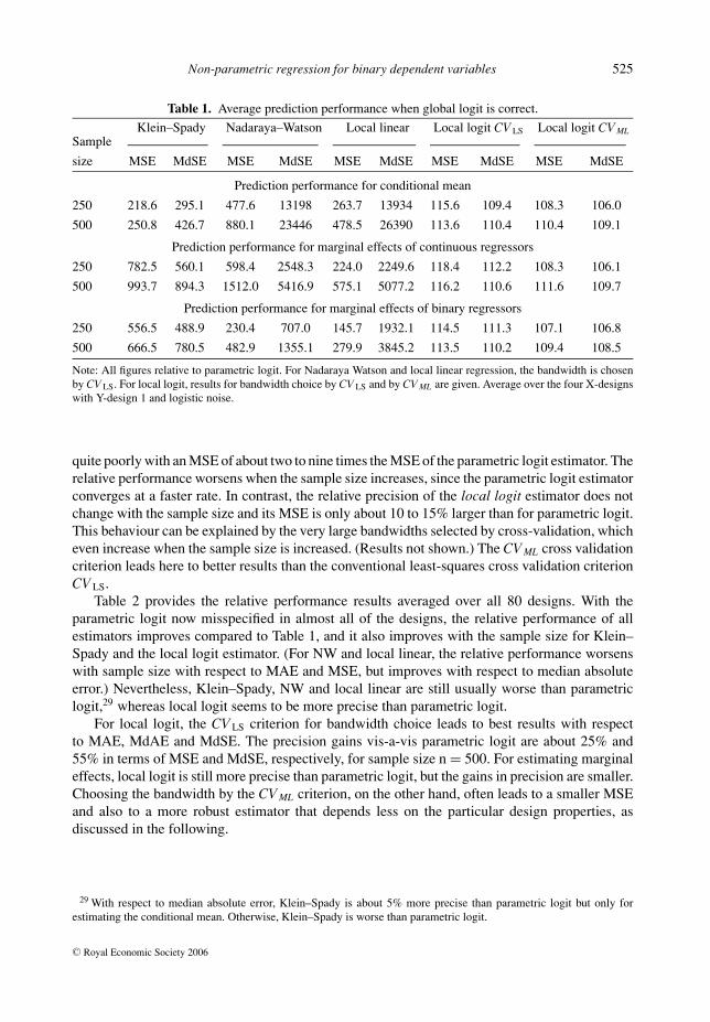
First, the relative performance of the various estimators in those designs where the parametriclogit model is correctly specified is examined in Table 1. These are the four X-designs withY-design 1 and logistic noise, and Table 1 gives the average over these four designs for samplesize 250 and 500, respectively. The first two rows of Table 1 contain the results for estimating theconditional mean E[Y|X]. Klein–Spady, Nadaraya–Watson and local linear regression perform
26 Four X-designs, five Y-designs and four noise variants.27 One hundred replications for each design.28 Hence, numbers below 100 indicate an improvement over parametric logit regression, whereas numbers above indicate
a worse performance.
C© Royal Economic Society 2006
Non-parametric regression for binary dependent variables 525
Table 1. Average prediction performance when global logit is correct.
Klein–Spady Nadaraya–Watson Local linear Local logit CV LS Local logit CV MLSample
size MSE MdSE MSE MdSE MSE MdSE MSE MdSE MSE MdSE
Prediction performance for conditional mean
250 218.6 295.1 477.6 13198 263.7 13934 115.6 109.4 108.3 106.0
500 250.8 426.7 880.1 23446 478.5 26390 113.6 110.4 110.4 109.1
Prediction performance for marginal effects of continuous regressors
250 782.5 560.1 598.4 2548.3 224.0 2249.6 118.4 112.2 108.3 106.1
500 993.7 894.3 1512.0 5416.9 575.1 5077.2 116.2 110.6 111.6 109.7
Prediction performance for marginal effects of binary regressors
250 556.5 488.9 230.4 707.0 145.7 1932.1 114.5 111.3 107.1 106.8
500 666.5 780.5 482.9 1355.1 279.9 3845.2 113.5 110.2 109.4 108.5
Note: All figures relative to parametric logit. For Nadaraya Watson and local linear regression, the bandwidth is chosenby CV LS. For local logit, results for bandwidth choice by CV LS and by CV ML are given. Average over the four X-designswith Y-design 1 and logistic noise.
quite poorly with an MSE of about two to nine times the MSE of the parametric logit estimator. Therelative performance worsens when the sample size increases, since the parametric logit estimatorconverges at a faster rate. In contrast, the relative precision of the local logit estimator does notchange with the sample size and its MSE is only about 10 to 15% larger than for parametric logit.This behaviour can be explained by the very large bandwidths selected by cross-validation, whicheven increase when the sample size is increased. (Results not shown.) The CV ML cross validationcriterion leads here to better results than the conventional least-squares cross validation criterionCV LS.
Table 2 provides the relative performance results averaged over all 80 designs. With theparametric logit now misspecified in almost all of the designs, the relative performance of allestimators improves compared to Table 1, and it also improves with the sample size for Klein–Spady and the local logit estimator. (For NW and local linear, the relative performance worsenswith sample size with respect to MAE and MSE, but improves with respect to median absoluteerror.) Nevertheless, Klein–Spady, NW and local linear are still usually worse than parametriclogit,29 whereas local logit seems to be more precise than parametric logit.
For local logit, the CV LS criterion for bandwidth choice leads to best results with respectto MAE, MdAE and MdSE. The precision gains vis-a-vis parametric logit are about 25% and55% in terms of MSE and MdSE, respectively, for sample size n = 500. For estimating marginaleffects, local logit is still more precise than parametric logit, but the gains in precision are smaller.Choosing the bandwidth by the CV ML criterion, on the other hand, often leads to a smaller MSEand also to a more robust estimator that depends less on the particular design properties, asdiscussed in the following.
29 With respect to median absolute error, Klein–Spady is about 5% more precise than parametric logit but only forestimating the conditional mean. Otherwise, Klein–Spady is worse than parametric logit.
C© Royal Economic Society 2006
526 Markus Frolich
Table 2. Average prediction performance over all designs.
Klein–Spady Nadaraya Watson Local linear Local logit CV LS Local logit CV MLSample
size MSE MdSE MSE MdSE MSE MdSE MSE MdSE MSE MdSE
Prediction performance for conditional mean
250 128.4 104.1 202.8 >10000 132.8 >10000 85.5 53.7 84.7 61.6
500 118.0 104.6 273.4 >10000 175.0 >10000 75.3 45.5 75.7 51.8
Prediction performance for marginal effects of continuous regressors
250 254.0 287.4 201.3 >10000 129.0 >10000 93.1 77.5 91.7 81.6
500 204.6 257.5 284.6 >10000 165.7 >10000 86.1 69.8 86.0 77.1
Prediction performance for marginal effects of binary regressors
250 227.8 212.9 134.7 >10000 112.4 >10000 103.9 74.0 99.4 80.1
500 186.0 192.8 172.3 2057 132.9 >10000 99.1 63.9 94.4 70.6
Note: All figures relative to parametric logit. For Nadaraya Watson and local linear regression, the bandwidth is chosenby CV LS. For local logit, results for bandwidth choice by CV LS and by CV ML are given. Average over all 80 designs.
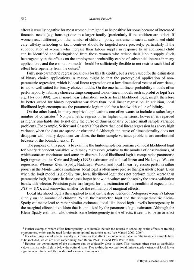
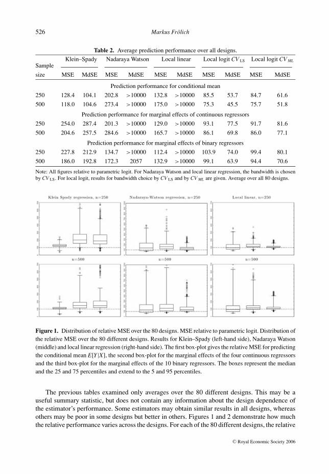
Figure 1. Distribution of relative MSE over the 80 designs. MSE relative to parametric logit. Distribution ofthe relative MSE over the 80 different designs. Results for Klein–Spady (left-hand side), Nadaraya Watson(middle) and local linear regression (right-hand side). The first box-plot gives the relative MSE for predictingthe conditional mean E[Y|X], the second box-plot for the marginal effects of the four continuous regressorsand the third box-plot for the marginal effects of the 10 binary regressors. The boxes represent the medianand the 25 and 75 percentiles and extend to the 5 and 95 percentiles.
The previous tables examined only averages over the 80 different designs. This may be auseful summary statistic, but does not contain any information about the design dependence ofthe estimator’s performance. Some estimators may obtain similar results in all designs, whereasothers may be poor in some designs but better in others. Figures 1 and 2 demonstrate how muchthe relative performance varies across the designs. For each of the 80 different designs, the relative
C© Royal Economic Society 2006
Non-parametric regression for binary dependent variables 527
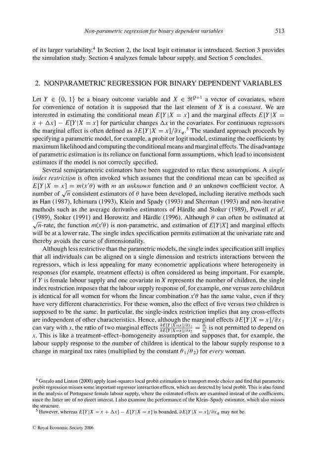
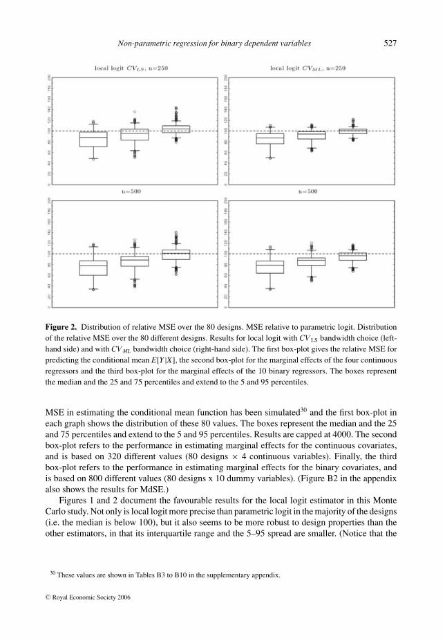
Figure 2. Distribution of relative MSE over the 80 designs. MSE relative to parametric logit. Distributionof the relative MSE over the 80 different designs. Results for local logit with CV LS bandwidth choice (left-hand side) and with CV ML bandwidth choice (right-hand side). The first box-plot gives the relative MSE forpredicting the conditional mean E[Y|X], the second box-plot for the marginal effects of the four continuousregressors and the third box-plot for the marginal effects of the 10 binary regressors. The boxes representthe median and the 25 and 75 percentiles and extend to the 5 and 95 percentiles.
MSE in estimating the conditional mean function has been simulated30 and the first box-plot ineach graph shows the distribution of these 80 values. The boxes represent the median and the 25and 75 percentiles and extend to the 5 and 95 percentiles. Results are capped at 4000. The secondbox-plot refers to the performance in estimating marginal effects for the continuous covariates,and is based on 320 different values (80 designs × 4 continuous variables). Finally, the thirdbox-plot refers to the performance in estimating marginal effects for the binary covariates, andis based on 800 different values (80 designs x 10 dummy variables). (Figure B2 in the appendixalso shows the results for MdSE.)
Figures 1 and 2 document the favourable results for the local logit estimator in this MonteCarlo study. Not only is local logit more precise than parametric logit in the majority of the designs(i.e. the median is below 100), but it also seems to be more robust to design properties than theother estimators, in that its interquartile range and the 5–95 spread are smaller. (Notice that the
30 These values are shown in Tables B3 to B10 in the supplementary appendix.
C© Royal Economic Society 2006

528 Markus Frolich
scaling of the ordinate varies between the estimators, e.g. the maximum value is close to 700 forthe Klein–Spady estimator but much smaller for local logit.)
The Klein–Spady estimator performs clearly worse than parametric logit in the majority of thedesigns, particularly when estimating marginal effects. Its behaviour improves with the samplesize, but at n = 500 it is still worse than parametric logit.31
For Nadaraya–Watson the results are even worse, with a very large relative MSE in a numberof designs and a spread increasing with sample size. In terms of MdSE, the Nadaraya–Watsonestimator performs very poorly.32 The results are less extreme for the marginal effects, but stillvery large. Hence, in terms of median prediction performance, Nadaraya–Watson can be veryunreliable.
These findings are similar for local linear regression. With respect to MSE, local linearregression behaves better than Nadaraya–Watson, and its MSE varies less with the simulationdesign. For predicting the conditional mean, it is slightly more precise than parametric logit, andfor the marginal effects it performs better than Klein–Spady. In terms of MdSE, however, it canoften be very imprecise. The finding that local linear regression performs extremely badly withrespect to MdSE but less badly in terms of MSE indicates that local linear regression producesdisproportionately many small errors. This could be related to the non-differentiability of the localmodel, which caps the estimates at 0 and 1. This produces rather many extreme predictions of0 and 1, whereas in the true data generating processes E[Y |X ] ∈ {0, 1} occurs with probabilityzero.
The results for local logit are shown in Figure 2. In the majority of the designs, local logitis more precise than parametric logit, particularly for the conditional mean function. Comparingbandwidth selection by CV LS or by CV ML, it seems that CV ML leads to a smaller spread over thedesigns. Particularly for n = 250, the interquartile range is smaller with CV ML than CV LS. Thisholds with respect to MSE as well as MdSE. Although the ranking of CV LS and CV ML with respectto the average performance over the 80 designs is ambiguous (see Table A2, the CV ML criterionled on average to a higher MAE, MdAE and MdSE but a smaller MSE), the CV ML criterionclearly reduced the variance in the performance over the 80 designs: the standard deviation overthe 80 designs is smaller for all the four performance measures MAE, MdAE, MSE and MdSE.Although the differences are not very large, this seems to indicate that the CV ML criterion makesthe local logit estimator more robust to the particular design properties.33
4. HETEROGENEOUS FEMALE LABOUR SUPPLY
The previous section indicated that local likelihood logit can work well even in higher-dimensionalsettings. In this section, local logit is applied to analyze female labour supply. Determinants offemale labour supply have since long been of interest to economists, arguing about the need forsubsidized child care or all-day schooling. As confirmed by many studies, female labour force
31 These findings hold with respect to MSE as well as MdSE, but with a much larger spread for MdSE. In some designs,the relative MdSE is very large whereas it is very small in others.
32 In more than 20 of the 80 designs the predictions of E[Y}X] are more than 40 times less precise than for parametriclogit. (The results are capped at 4000) At the median of the 80 designs, the MdSE is larger than 400. These findings aresimilar, but somewhat less extreme, with respect to median absolute error.
33 It should be kept in mind that precision is measured relative to the parametric logit estimator.
C© Royal Economic Society 2006
Non-parametric regression for binary dependent variables 529
participation generally decreases with the number of children and particularly if these children areyoung. For policy considerations, however, it would be relevant to know whether all women adjusttheir labour supply in the same way as a reaction on family size or whether some sub-populationsreact differently. Particularly, for some women, labour supply might be inelastic to family size,whereas for others it might even increase as a reaction on an additional child, e.g. because ofincreased financial needs. If women’s reaction on family size is heterogeneous, the provision ofchild care subsidies, tax incentives, etc. should be targeted more precisely than if it were largelyhomogeneous. Therefore, in the analysis of female labour supply, not only should mean effectsbe estimated but their distribution should also be estimated.
To assess heterogeneity in women’s response to family size, the labour force participation ofmarried Portuguese women is analyzed by a reduced form labour supply model. The data are takenfrom Martins (2001) and consist of 2339 women of whom 60% had been working in 1991. Fiveexplanatory variables are available: age, years of education, husband’s monthly wage, number ofchildren below the age of 4 and number of children 4 to 18 years old. Tables A1 and A2 in theAppendix contain descriptive statistics.
For each woman her employment probability P(Y = 1|X i ) given her characteristics X i isestimated, where Y denotes employment status (1 employed, 0 non-employed). In addition, themarginal effects of the characteristics X i on employment are estimated, in particular the effects ofthe number of children. The effect of an additional child on the employment probability dependson all characteristics X i and thus differs from woman to woman.34
The employment probabilities P(Y = 1|X i ) and the marginal effects are estimated byparametric logit, local logit and Klein–Spady. A bandwidth of 0.1 times the standard deviationof the index xβ was selected for the Klein Spady estimator, and for scale normalization the firstcoefficient is fixed. For the local logit estimator, all five variables (plus a constant) enter in the localmodel and in the kernel weighting. The local logit specification is economically appealing as itincorporates monotonicity, decreasing marginal effects and non-saturation. From a simple utility-maximizing labour supply model, the labour supply should usually decrease with the number ofchildren but the effect of an additional child should diminish (e.g. due to returns to scale in childrearing and home production). Nevertheless, the marginal effect should not fall to zero. Theseimplications of the simple model are not incorporated in the local constant or the capped locallinear model.
For the kernel weighting, the five regressors are split into two groups: age, education andhusband’s wage income are treated as continuous variables. The optimal bandwidth for each ofthese three variables is supposed to be proportional to its standard deviation. By imposing therestrictions that hage = h Std(age), heducation = h Std(education) and hwage = h Std(wage), it sufficesto estimate a single bandwidth h, while at the same time ensuring that the local neighbourhoodsare larger for regressors that display more variation. In the actual implementation of the estimator,this restriction is accommodated by scaling the continuous regressors to mean zero and varianceone. The second group of regressors consists of the number of children 0–3 years and 4–18 yearsold. These two variables are treated as ordered discrete. The same bandwidth value is used for
34 Note that the estimated effects of children can be interpreted as causal only if the number of children is exogenousgiven the other characteristics. If some confounding variables that affect both the number of children and the inclinationto work are missing, the estimated employment effects are a mixture of the proper causal effect and a selection effect,(see Heckman 1990; Manski 1993). This would change the interpretation of the estimated effects but not the comparisonof the different estimators’ ability in detecting heterogeneous effects.
C© Royal Economic Society 2006
530 Markus Frolich
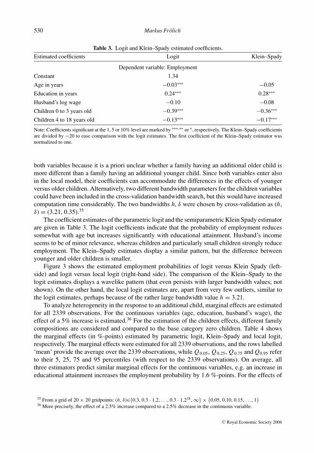
Table 3. Logit and Klein–Spady estimated coefficients.
Estimated coefficients Logit Klein–Spady
Dependent variable: Employment
Constant 1.34
Age in years −0.03∗∗∗ −0.05
Education in years 0.24∗∗∗ 0.28∗∗∗
Husband’s log wage −0.10 −0.08
Children 0 to 3 years old −0.39∗∗∗ −0.36∗∗∗
Children 4 to 18 years old −0.13∗∗∗ −0.17∗∗∗
Note: Coefficients significant at the 1, 5 or 10% level are marked by ∗∗∗,∗∗ or ∗, respectively. The Klein–Spady coefficientsare divided by −20 to ease comparison with the logit estimates. The first coefficient of the Klein–Spady estimator wasnormalized to one.
both variables because it is a priori unclear whether a family having an additional older child ismore different than a family having an additional younger child. Since both variables enter alsoin the local model, their coefficients can accommodate the differences in the effects of youngerversus older children. Alternatively, two different bandwidth parameters for the children variablescould have been included in the cross-validation bandwidth search, but this would have increasedcomputation time considerably. The two bandwidths h, δ were chosen by cross-validation as (h,δ) = (3.21, 0.35).35
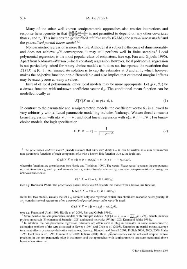
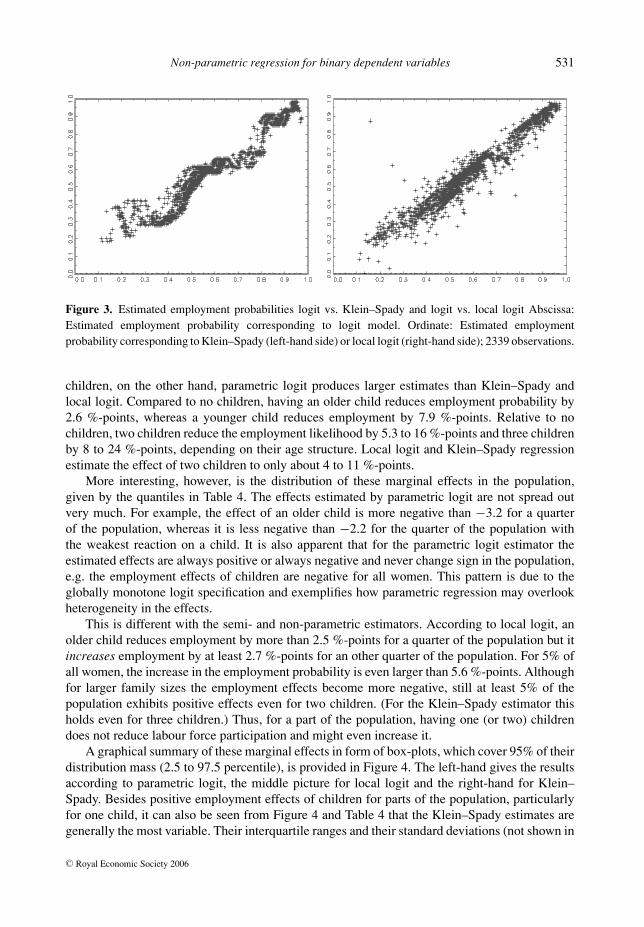
The coefficient estimates of the parametric logit and the semiparametric Klein Spady estimatorare given in Table 3. The logit coefficients indicate that the probability of employment reducessomewhat with age but increases significantly with educational attainment. Husband’s incomeseems to be of minor relevance, whereas children and particularly small children strongly reduceemployment. The Klein–Spady estimates display a similar pattern, but the difference betweenyounger and older children is smaller.
Figure 3 shows the estimated employment probabilities of logit versus Klein Spady (left-side) and logit versus local logit (right-hand side). The comparison of the Klein–Spady to thelogit estimates displays a wavelike pattern (that even persists with larger bandwidth values; notshown). On the other hand, the local logit estimates are, apart from very few outliers, similar tothe logit estimates, perhaps because of the rather large bandwidth value h = 3.21.
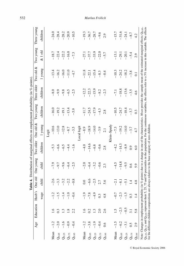
To analyze heterogeneity in the response to an additional child, marginal effects are estimatedfor all 2339 observations. For the continuous variables (age, education, husband’s wage), theeffect of a 5% increase is estimated.36 For the estimation of the children effects, different familycompositions are considered and compared to the base category zero children. Table 4 showsthe marginal effects (in %-points) estimated by parametric logit, Klein–Spady and local logit,respectively. The marginal effects were estimated for all 2339 observations, and the rows labelled‘mean’ provide the average over the 2339 observations, while Q0.05, Q0.25, Q0.75 and Q0.95 referto their 5, 25, 75 and 95 percentiles (with respect to the 2339 observations). On average, allthree estimators predict similar marginal effects for the continuous variables, e.g. an increase ineducational attainment increases the employment probability by 1.6 %-points. For the effects of
35 From a grid of 20 × 20 gridpoints: (h, δ)∈{0.3, 0.3 · 1.2, . . ., 0.3 · 1.218, ∞} × {0.05, 0.10, 0.15, . . ., 1}36 More precisely, the effect of a 2.5% increase compared to a 2.5% decrease in the continuous variable.
C© Royal Economic Society 2006
Non-parametric regression for binary dependent variables 531
Figure 3. Estimated employment probabilities logit vs. Klein–Spady and logit vs. local logit Abscissa:Estimated employment probability corresponding to logit model. Ordinate: Estimated employmentprobability corresponding to Klein–Spady (left-hand side) or local logit (right-hand side); 2339 observations.
children, on the other hand, parametric logit produces larger estimates than Klein–Spady andlocal logit. Compared to no children, having an older child reduces employment probability by2.6 %-points, whereas a younger child reduces employment by 7.9 %-points. Relative to nochildren, two children reduce the employment likelihood by 5.3 to 16 %-points and three childrenby 8 to 24 %-points, depending on their age structure. Local logit and Klein–Spady regressionestimate the effect of two children to only about 4 to 11 %-points.
More interesting, however, is the distribution of these marginal effects in the population,given by the quantiles in Table 4. The effects estimated by parametric logit are not spread outvery much. For example, the effect of an older child is more negative than −3.2 for a quarterof the population, whereas it is less negative than −2.2 for the quarter of the population withthe weakest reaction on a child. It is also apparent that for the parametric logit estimator theestimated effects are always positive or always negative and never change sign in the population,e.g. the employment effects of children are negative for all women. This pattern is due to theglobally monotone logit specification and exemplifies how parametric regression may overlookheterogeneity in the effects.
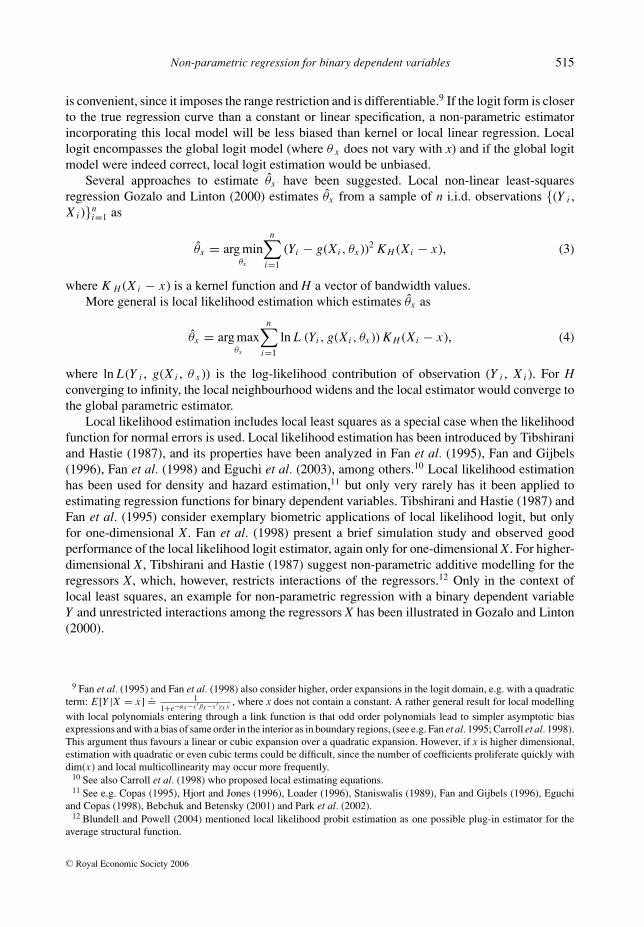
This is different with the semi- and non-parametric estimators. According to local logit, anolder child reduces employment by more than 2.5 %-points for a quarter of the population but itincreases employment by at least 2.7 %-points for an other quarter of the population. For 5% ofall women, the increase in the employment probability is even larger than 5.6 %-points. Althoughfor larger family sizes the employment effects become more negative, still at least 5% of thepopulation exhibits positive effects even for two children. (For the Klein–Spady estimator thisholds even for three children.) Thus, for a part of the population, having one (or two) childrendoes not reduce labour force participation and might even increase it.
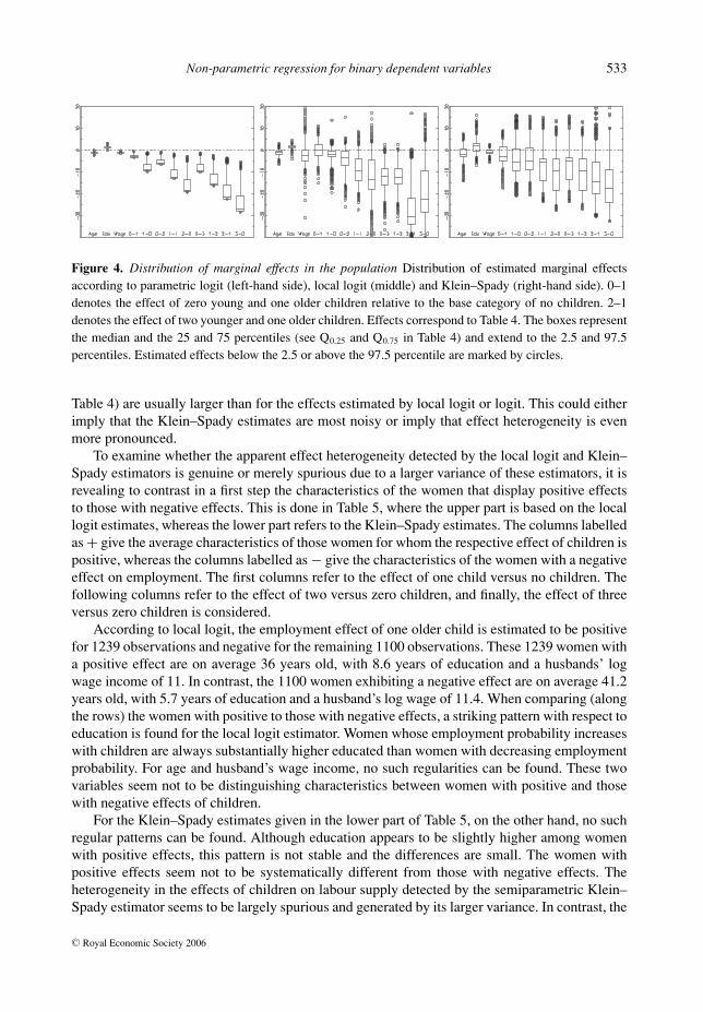
A graphical summary of these marginal effects in form of box-plots, which cover 95% of theirdistribution mass (2.5 to 97.5 percentile), is provided in Figure 4. The left-hand gives the resultsaccording to parametric logit, the middle picture for local logit and the right-hand for Klein–Spady. Besides positive employment effects of children for parts of the population, particularlyfor one child, it can also be seen from Figure 4 and Table 4 that the Klein–Spady estimates aregenerally the most variable. Their interquartile ranges and their standard deviations (not shown in
C© Royal Economic Society 2006
532 Markus Frolich
Ta
ble
4.
Dis
trib
utio
nof
mar
gina
leff
ects
onem
ploy
men
tpro
babi
lity
(in
%-p
oint
s).
Age
Edu
catio
nH
usb’
sO
neol
dO
neyo
ung
Two
olde
rO
neol
d&
Two
youn
gT
hree
olde
rTw
ool
d&
Two
youn
gT
hree
youn
g
wag
ech
ildch
ildch
ildre
n1
youn
gch
ildre
nch
ildre
n1
youn
g&
1ol
dch
ildre
n
Log
it
Mea
n−1
.21.
6−1
.2−2
.6−7
.9−5
.3−1
0.6
−16.
0−8
.0−1
3.4
−18.
7−2
4.0
Q0.
05−2
.00.
3−1
.5−3
.3−9
.7−6
.6−1
3.0
−19.
2−9
.9−1
6.2
−22.
4−2
8.4
Q0.
25−1
.61.
3−1
.4−3
.2−9
.6−6
.5−1
2.8
−19.
1−9
.8−1
6.0
−22.
2−2
8.2
Q0.
75−0
.91.
8−1
.0−2
.2−6
.4−4
.4−8
.7−1
3.4
−6.5
−11.
0−1
6.0
−20.
9
Q0.
95−0
.42.
2−0
.4−0
.8−2
.5−1
.6−3
.5−5
.9−2
.5−4
.7−7
.3−1
0.5
Loc
allo
git
Mea
n−1
.21.
6−1
.90.
0−2
.0−4
.0−8
.9−1
1.7
−12.
2−1
1.8
−27.
1−1
9.3
Q0.
05−3
.80.
2−7
.8−6
.6−6
.4−1
4.6
−18.
9−2
4.5
−22.
3−2
2.1
−37.
7−3
6.7
Q0.
25−1
.91.
3−4
.9−2
.5−3
.2−6
.8−1
4.0
−17.
9−1
5.9
−15.
4−3
3.9
−28.
7
Q0.
75−0
.42.
00.
32.
7−0
.6−0
.6−3
.9−4
.3−8
.2−8
.3−2
2.0
−9.6
Q0.
950.
62.
64.
85.
62.
32.
82.
12.
8−2
.3−0
.4−5
.72.
9
Kle
in–S
pady
Mea
n−1
.51.
5−0
.7−2
.1−4
.5−4
.2−7
.3−1
0.5
−7.1
−10.
3−1
3.1
−15.
7
Q0.
05−6
.2−2
.3−2
.3−8
.1−1
4.8
−14.
3−1
9.2
−24.
7−1
8.8
−24.
2−2
9.1
−31.
6
Q0.
25−3
.1−0
.5−1
.5−5
.1−9
.5−8
.9−1
4.0
−18.
4−1
3.6
−18.
2−2
0.1
−24.
1
Q0.
750.
53.
10.
31.
40.
60.
9−3
.7−3
.7−3
.5−3
.8−5
.4−8
.7
Q0.
952.
95.
81.
44.
85.
96.
04.
70.
34.
60.
12.
94.
2
Not
e:C
hang
esin
empl
oym
entp
roba
bilit
y(i
n%
-poi
nts)
due
toa
chan
gein
one
ofth
ech
arac
teri
stic
s.M
ean
prov
ides
the
sam
ple
mea
nof
the
estim
ated
mar
gina
leff
ects
;Q0.
05,
Q0.
25,Q
0.75
and
Q0.
95re
pres
entt
heir
5,25
,75
and
95pe
rcen
tiles
inth
epo
pula
tion.
For
the
cont
inuo
usva
riab
les,
the
effe
cts
refe
rto
a5%
incr
ease
inth
isva
riab
le.T
heef
fect
sfo
rth
edi
ffer
entc
hild
ren
com
posi
tions
are
alw
ays
rela
tive
toth
eba
seca
tego
ryof
zero
child
ren.
C© Royal Economic Society 2006
Non-parametric regression for binary dependent variables 533
Figure 4. Distribution of marginal effects in the population Distribution of estimated marginal effectsaccording to parametric logit (left-hand side), local logit (middle) and Klein–Spady (right-hand side). 0–1denotes the effect of zero young and one older children relative to the base category of no children. 2–1denotes the effect of two younger and one older children. Effects correspond to Table 4. The boxes representthe median and the 25 and 75 percentiles (see Q0.25 and Q0.75 in Table 4) and extend to the 2.5 and 97.5percentiles. Estimated effects below the 2.5 or above the 97.5 percentile are marked by circles.
Table 4) are usually larger than for the effects estimated by local logit or logit. This could eitherimply that the Klein–Spady estimates are most noisy or imply that effect heterogeneity is evenmore pronounced.
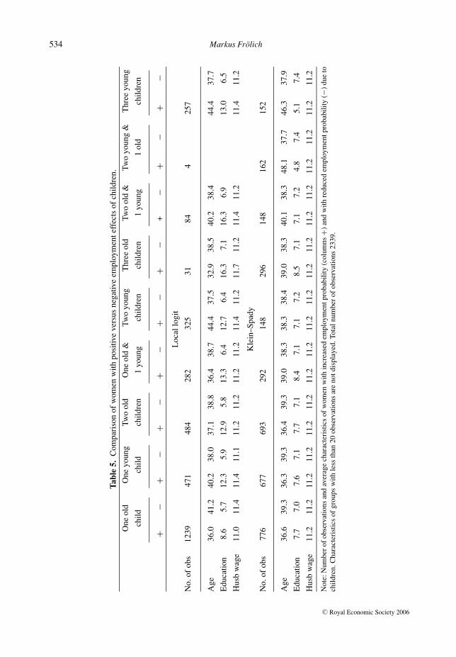
To examine whether the apparent effect heterogeneity detected by the local logit and Klein–Spady estimators is genuine or merely spurious due to a larger variance of these estimators, it isrevealing to contrast in a first step the characteristics of the women that display positive effectsto those with negative effects. This is done in Table 5, where the upper part is based on the locallogit estimates, whereas the lower part refers to the Klein–Spady estimates. The columns labelledas + give the average characteristics of those women for whom the respective effect of children ispositive, whereas the columns labelled as − give the characteristics of the women with a negativeeffect on employment. The first columns refer to the effect of one child versus no children. Thefollowing columns refer to the effect of two versus zero children, and finally, the effect of threeversus zero children is considered.
According to local logit, the employment effect of one older child is estimated to be positivefor 1239 observations and negative for the remaining 1100 observations. These 1239 women witha positive effect are on average 36 years old, with 8.6 years of education and a husbands’ logwage income of 11. In contrast, the 1100 women exhibiting a negative effect are on average 41.2years old, with 5.7 years of education and a husband’s log wage of 11.4. When comparing (alongthe rows) the women with positive to those with negative effects, a striking pattern with respect toeducation is found for the local logit estimator. Women whose employment probability increaseswith children are always substantially higher educated than women with decreasing employmentprobability. For age and husband’s wage income, no such regularities can be found. These twovariables seem not to be distinguishing characteristics between women with positive and thosewith negative effects of children.
For the Klein–Spady estimates given in the lower part of Table 5, on the other hand, no suchregular patterns can be found. Although education appears to be slightly higher among womenwith positive effects, this pattern is not stable and the differences are small. The women withpositive effects seem not to be systematically different from those with negative effects. Theheterogeneity in the effects of children on labour supply detected by the semiparametric Klein–Spady estimator seems to be largely spurious and generated by its larger variance. In contrast, the
C© Royal Economic Society 2006
534 Markus Frolich
Ta
ble
5.
Com
pari
son
ofw
omen
with
posi
tive
vers
usne
gativ
eem
ploy
men
teff
ects
ofch
ildre
n.
One
old
One
youn
gTw
ool
dO
neol
d&
Two
youn
gT
hree
old
Two
old
&Tw
oyo
ung
&T
hree
youn
g
child
child
child
ren
1yo
ung
child
ren
child
ren
1yo
ung
1ol
dch
ildre
n
+−
+−
+−
+−
+−
+−
+−
+−
+−
Loc
allo
git
No.
ofob
s12
3947
148
428
232
531
844
257
Age
36.0
41.2
40.2
38.0
37.1
38.8
36.4
38.7
44.4
37.5
32.9
38.5
40.2
38.4
44.4
37.7
Edu
catio
n8.
65.
712
.35.
912
.95.
813
.36.
412
.76.
416
.37.
116
.36.
913
.06.
5
Hus
bw
age
11.0
11.4
11.4
11.1
11.2
11.2
11.2
11.2
11.4
11.2
11.7
11.2
11.4
11.2
11.4
11.2
Kle
in–S
pady
No.
ofob
s77
667
769
329
214
829
614
816
215
2
Age
36.6
39.3
36.3
39.3
36.4
39.3
39.0
38.3
38.3
38.4
39.0
38.3
40.1
38.3
48.1
37.7
46.3
37.9
Edu
catio
n7.
77.
07.
67.
17.
77.
18.
47.
17.
17.
28.
57.
17.
17.
24.
87.
45.
17.
4
Hus
bw
age
11.2
11.2
11.2
11.2
11.2
11.2
11.2
11.2
11.2
11.2
11.2
11.2
11.2
11.2
11.2
11.2
11.2
11.2
Not
e:N
umbe
rof
obse
rvat
ions
and
aver
age
char
acte
rist
ics
ofw
omen
with
incr
ease
dem
ploy
men
tpro
babi
lity
(col
umns
+)an
dw
ithre
duce
dem
ploy
men
tpro
babi
lity
(−)
due
toch
ildre
n.C
hara
cter
istic
sof
grou
psw
ithle
ssth
an20
obse
rvat
ions
are
notd
ispl
ayed
.Tot
alnu
mbe
rof
obse
rvat
ions
2339
.
C© Royal Economic Society 2006
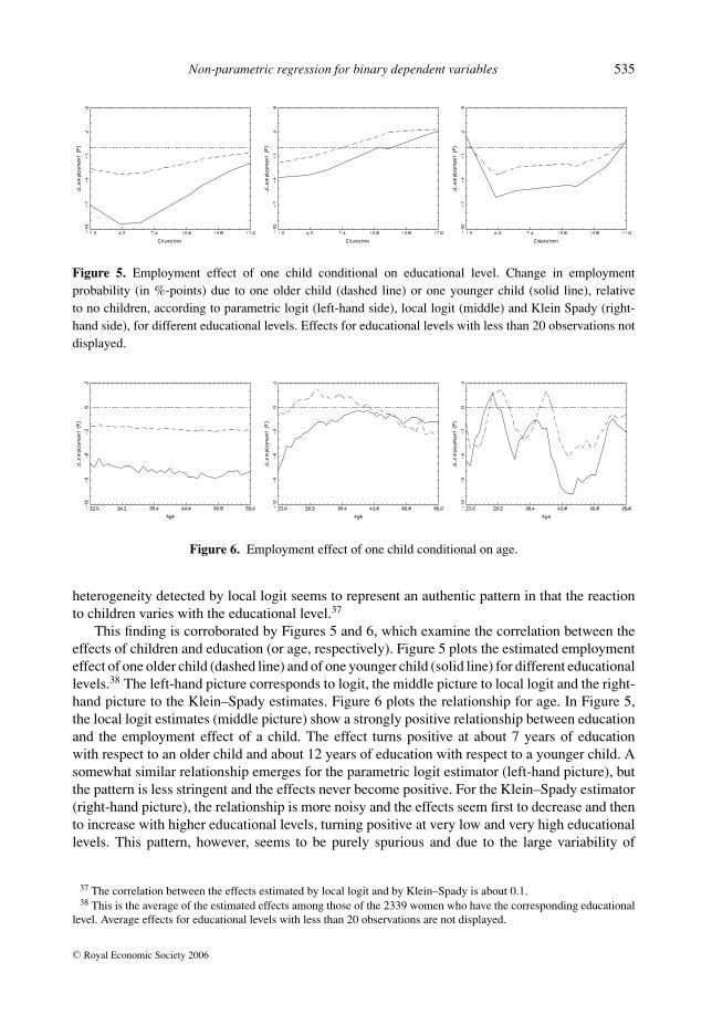
Non-parametric regression for binary dependent variables 535
Figure 5. Employment effect of one child conditional on educational level. Change in employmentprobability (in %-points) due to one older child (dashed line) or one younger child (solid line), relativeto no children, according to parametric logit (left-hand side), local logit (middle) and Klein Spady (right-hand side), for different educational levels. Effects for educational levels with less than 20 observations notdisplayed.
Figure 6. Employment effect of one child conditional on age.
heterogeneity detected by local logit seems to represent an authentic pattern in that the reactionto children varies with the educational level.37
This finding is corroborated by Figures 5 and 6, which examine the correlation between theeffects of children and education (or age, respectively). Figure 5 plots the estimated employmenteffect of one older child (dashed line) and of one younger child (solid line) for different educationallevels.38 The left-hand picture corresponds to logit, the middle picture to local logit and the right-hand picture to the Klein–Spady estimates. Figure 6 plots the relationship for age. In Figure 5,the local logit estimates (middle picture) show a strongly positive relationship between educationand the employment effect of a child. The effect turns positive at about 7 years of educationwith respect to an older child and about 12 years of education with respect to a younger child. Asomewhat similar relationship emerges for the parametric logit estimator (left-hand picture), butthe pattern is less stringent and the effects never become positive. For the Klein–Spady estimator(right-hand picture), the relationship is more noisy and the effects seem first to decrease and thento increase with higher educational levels, turning positive at very low and very high educationallevels. This pattern, however, seems to be purely spurious and due to the large variability of
37 The correlation between the effects estimated by local logit and by Klein–Spady is about 0.1.38 This is the average of the estimated effects among those of the 2339 women who have the corresponding educational
level. Average effects for educational levels with less than 20 observations are not displayed.
C© Royal Economic Society 2006
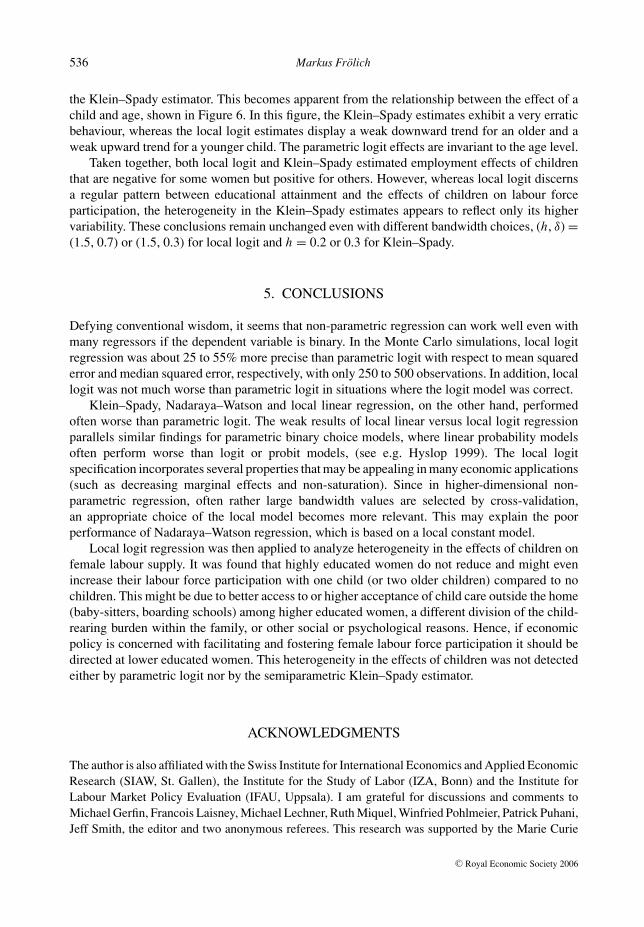
536 Markus Frolich
the Klein–Spady estimator. This becomes apparent from the relationship between the effect of achild and age, shown in Figure 6. In this figure, the Klein–Spady estimates exhibit a very erraticbehaviour, whereas the local logit estimates display a weak downward trend for an older and aweak upward trend for a younger child. The parametric logit effects are invariant to the age level.
Taken together, both local logit and Klein–Spady estimated employment effects of childrenthat are negative for some women but positive for others. However, whereas local logit discernsa regular pattern between educational attainment and the effects of children on labour forceparticipation, the heterogeneity in the Klein–Spady estimates appears to reflect only its highervariability. These conclusions remain unchanged even with different bandwidth choices, (h, δ) =(1.5, 0.7) or (1.5, 0.3) for local logit and h = 0.2 or 0.3 for Klein–Spady.
5. CONCLUSIONS
Defying conventional wisdom, it seems that non-parametric regression can work well even withmany regressors if the dependent variable is binary. In the Monte Carlo simulations, local logitregression was about 25 to 55% more precise than parametric logit with respect to mean squarederror and median squared error, respectively, with only 250 to 500 observations. In addition, locallogit was not much worse than parametric logit in situations where the logit model was correct.
Klein–Spady, Nadaraya–Watson and local linear regression, on the other hand, performedoften worse than parametric logit. The weak results of local linear versus local logit regressionparallels similar findings for parametric binary choice models, where linear probability modelsoften perform worse than logit or probit models, (see e.g. Hyslop 1999). The local logitspecification incorporates several properties that may be appealing in many economic applications(such as decreasing marginal effects and non-saturation). Since in higher-dimensional non-parametric regression, often rather large bandwidth values are selected by cross-validation,an appropriate choice of the local model becomes more relevant. This may explain the poorperformance of Nadaraya–Watson regression, which is based on a local constant model.
Local logit regression was then applied to analyze heterogeneity in the effects of children onfemale labour supply. It was found that highly educated women do not reduce and might evenincrease their labour force participation with one child (or two older children) compared to nochildren. This might be due to better access to or higher acceptance of child care outside the home(baby-sitters, boarding schools) among higher educated women, a different division of the child-rearing burden within the family, or other social or psychological reasons. Hence, if economicpolicy is concerned with facilitating and fostering female labour force participation it should bedirected at lower educated women. This heterogeneity in the effects of children was not detectedeither by parametric logit nor by the semiparametric Klein–Spady estimator.
ACKNOWLEDGMENTS
The author is also affiliated with the Swiss Institute for International Economics and Applied EconomicResearch (SIAW, St. Gallen), the Institute for the Study of Labor (IZA, Bonn) and the Institute forLabour Market Policy Evaluation (IFAU, Uppsala). I am grateful for discussions and comments toMichael Gerfin, Francois Laisney, Michael Lechner, Ruth Miquel, Winfried Pohlmeier, Patrick Puhani,Jeff Smith, the editor and two anonymous referees. This research was supported by the Marie Curie
C© Royal Economic Society 2006
Non-parametric regression for binary dependent variables 537
Individual Fellowship MEIF-CT-2004-006873, the Swiss National Science Foundation (project NSF4043-058311) and the Grundlagenforschungsfonds HSG (project G02110112).
REFERENCES
Bebchuk, J. and R. Betensky (2001). Local likelihood analysis of survival data with censored intermediateevents. Journal of American Statistical Association 96, 449–57.
Blundell, R. and J. Powell (2004). Endogeneity in semiparametric binary response models. Review ofEconomic Studies 71, 655–79.
Carroll, R., D. Ruppert and A. Welsh (1998). Local estimating equations. Journal of American StatisticalAssociation 93, 214–27.
Chen, X., O. Linton and I. van Keilegom (2003). Estimation of semiparametric models when the criterionfunction is not smooth. Econometrica 71, 1591–608.
Copas, J. (1995). Local likelihood based on kernel censoring. Journal of the Royal Statistical Society, SeriesB 57, 221–35.
Eguchi, S. and J. Copas (1998). A class of local likelihood methods and near-parametric asymptotics. Journalof Royal Statistical Society, Series B 60, 709–24.
Eguchi, S., T. Kim and B. Park (2003). Local likelihood method: a bridge over parametric and nonparametricregression. Journal of Nonparametric Statistics 15, 665–83.
Fan, J., M. Farmen and I. Gijbels (1998). Local Maximum Likelihood Estimation and Inference. Journal ofthe Royal Statistical Society, Series B 60, 591–608.
Fan, J. and I. Gijbels (1996). Local Polynomial Modeling and its Applications. Chapman and Hall, London.Fan, J., N. Heckman and M. Wand (1995). Local polynomial kernel regression for generalized linear models
and quasi-likelihood functions. Journal of the American Statistical Association 90, 141–50.Friedman, J. and W. Stuetzle (1981). Projection pursuit regression. Journal of American Statistical
Association 76, 817–23.Frolich, M. (2004). Finite sample properties of propensity-score matching and weighting estimators. The
Review of Economics and Statistics 86, 77–90.Frolich, M. (2005). Matching estimators and optimal bandwidth choice. Statistics and Computing 15, 197–
215.Frolich, M. (2006). Nonparametric IV estimation of local average treatment effects with covariates. Journal
of Econometrics (in press).Galindo, C., H. Liang, G. Kauermann and R. Carrol (2001). Bootstrap confidence intervals for local
likelihood, local estimating equations and varying coefficient models. Statistica Sinica 11, 121–34.
Gerfin, M. (1996). Parametric and semi-parametric estimation of the binary response model of labour marketparticipation. Journal of Applied Econometrics 11, 321–39.
Gozalo, P. and O. Linton (2000). Local nonlinear least squares: Using parametric information innonparametric regression. Journal of Econometrics 99, 63–106.
Hahn, J. (1998). On the role of the propensity score in efficient semiparametric estimation of averagetreatment effects. Econometrica 66, 315–31.
Han, A. (1987). Non-parametric analysis of a generalized regression model. Journal of Econometrics 35,303–16.
Hardle, W., M. Muller, S. Sperlich and A. Werwatz (2004). Nonparametric and Semiparametric Models.Springer, Heidelberg.
C© Royal Economic Society 2006
538 Markus Frolich
Hardle, W. and T. Stoker (1989). Investigating smooth multiple regression by the method of averagederivatives. Journal of American Statistical Association 84, 986–95.
Hastie, T. and R. Tibshirani (1990). Generalized Additive Models. Chapman and Hall, London.Heckman, J. (1990). Varieties of selection bias. American Economic Review, Papers and Proceedings 80,
313–18.Heckman, J., H. Ichimura and P. Todd (1998). Matching as an econometric evaluation estimator. Review of
Economic Studies 65, 261–94.Heckman, J., J. Smith and N. Clements (1997). Making the most out of programme evaluations and social
experiments: Accounting for heterogeneity in programme impacts. Review of Economic Studies 64, 487–535.
Hirano, K., G. Imbens and G. Ridder (2003). Efficient estimation of average treatment effects using theestimated propensity score. Econometrica 71, 1161–89.
Hjort, N. and M. Jones (1996). Locally parametric nonparametric density estimation. Annals of Statistics24, 1619–47.
Holland, P. (1986). Statistics and causal inference. Journal of American Statistical Association 81, 945–70.
Horowitz, J. and W. Hardle (1996). Direct semiparametric estimation of single-index models with discretecovariates. Journal of American Statistical Association 91, 1632–40.
Hyslop, D. (1999). State dependence, serial correlation and heterogeneity in intertemporal labor forceparticipation of married women. Econometrica 67, 1255–94.
Ichimura, H. (1993). Semiparametric least squares (SLS) and weighted SLS estimation of single-indexmodels. Journal of Econometrics 58, 71–120.
Imbens, G. (2004). Nonparametric estimation of average treatment effects under exogeneity: A review. TheReview of Economics and Statistics 86, 4–29.
Klein, R. and R. Spady (1993). An efficient semiparametric estimator for binary response models.Econometrica 61, 387–421.
Kuan, C. and H. White (1994). Artifical neural networks: An econometric perspective. Econometric Reviews13, 1–91.
Loader, C. (1996). Local likelihood density estimation. Annals of Statistics 24, 1602–18.Manski, C. (1993). The selection problem in econometrics and statistics. In. Eds. G. Maddala, C. Rao, and
H. Vinod. Handbook of Statistics. Elsevier Science Publishers, Amsterdam.Manski, C. (2000). Identification problems and decisions under ambiguity: Empirical analysis of treatment
response and normative analysis of treatment choice. Journal of Econometrics 95, 415–42.Manski, C. (2004). Statistical treatment rules for heterogeneous populations. Econometrica 72, 1221–46.Martins, M. (2001). Parametric and semiparametric estimation of sample selection models: An empirical
application to the female labour force in portugal. Journal of Applied Econometrics 16, 23–39.Newey, W. (1994). The asymptotic variance of semiparametric estimators. Econometrica 62, 1349–
82.Pagan, A. and A. Ullah (1999). Nonparametric Econometrics. Cambridge University Press, Cambridge.Park, B., W. Kim and M. Jones (2002). On local likelihood density estimation. Annals of Statistics 30,
1480–95.Pearl, J. (2000). Causality: Models, Reasoning and Inference. Cambridge University Press, Cambridge.Powell, J., J. Stock and T. Stoker (1989). Semiparametric estimation of index coefficients. Econometrica
57, 1403–30.Racine, J. and Q. Li (2004). Nonparametric estimation of regression functions with both categorical and
continuous data. Journal of Econometrics 119, 99–130.Robinson, P. (1998). Root-N consistent semiparametric regression. Econometrica 56, 931–54.
C© Royal Economic Society 2006
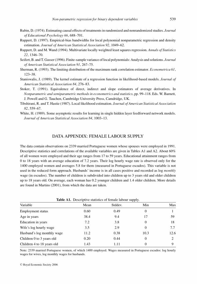
Non-parametric regression for binary dependent variables 539
Rubin, D. (1974). Estimating causal effects of treatments in randomized and nonrandomized studies. Journalof Educational Psychology 66, 688–701.
Ruppert, D. (1997). Empirical-bias bandwidths for local polynomial nonparametric regression and densityestimation. Journal of American Statistical Association 92, 1049–62.
Ruppert, D. and M. Wand (1994). Multivariate locally weighted least squares regression. Annals of Statistics22, 1346–70.
Seifert, B. and T. Gasser (1996). Finite-sample variance of local polynomials: Analysis and solutions. Journalof American Statistical Association 91, 267–75.
Sherman, R. (1993). The limiting distribution of the maximum rank correlation estimator. Econometrica 61,123–38.
Staniswalis, J. (1989). The kernel estimate of a regression function in likelihood-based models. Journal ofAmerican Statistical Association 84, 276–83.
Stoker, T. (1991). Equivalence of direct, indirect and slope estimators of average derivatives. InNonparametric and semiparametric methods in econometrics and statistics, pp. 99–118. Eds. W. Barnett,J. Powell and G. Tauchen, Cambridge University Press, Camdridge, UK.
Tibshirani, R. and T. Hastie (1987). Local likelihood estimation. Journal of American Statistical Association82, 559–67.
White, H. (1989). Some asymptotic results for learning in single hidden layer feedforward network models.Journal of American Statistical Association 84, 1003–13.
DATA APPENDIX: FEMALE LABOUR SUPPLY
The data contain observations on 2339 married Portuguese women whose spouses were employed in 1991.Descriptive statistics and correlations of the available variables are given in Tables A1 and A2. About 60%of all women were employed and their age ranges from 17 to 59 years. Educational attainment ranges from0 to 18 years with an average education of 7.2 years. Their log hourly wage rate is observed only for the1400 employed women and averages 5.8 for them (measured in Portuguese escudos). This variable is notused in the reduced form approach. Husbands’ income is in all cases positive and recorded as log monthlywage (in escudos). The number of children is subdivided into children up to 3 years old and older childrenup to 18 years old. On average, each woman has 0.2 younger children and 1.4 older children. More detailsare found in Martins (2001), from which the data are taken.
Table A1. Descriptive statistics of female labour supply.
Variable Mean Stddev. Min Max
Employment status 0.60 0.49 0 1
Age in years 38.4 9.4 17 59
Education in years 7.2 3.8 0 18
Wife’s log hourly wage 3.5 2.9 0 7.7
Husband’s log monthly wage 11.2 0.38 10.3 12.6
Children 0 to 3 years old 0.20 0.44 0 2
Children 4 to 18 years old 1.43 1.11 0 9
Note: 2339 married Portuguese women, of which 1400 employed. Wages measured in Portuguese escudos: log hourlywages for wives, log monthly wages for husbands.
C© Royal Economic Society 2006

540 Markus Frolich
Table A2. Correlation matrix.
Age Education Husb’ wage Children 0−3 Children 4–18
Employment status −0.16 0.36 0.09 0.03 −0.12
Age in years −0.14 0.07 −0.41 0.23
Education in years 0.31 0.08 −0.13
Husband’s wage −0.05 −0.02
Children 0 to 3 years old −0.24
C© Royal Economic Society 2006