Embed Size (px)
Citation preview

Non-smooth Non-convex Bregman Minimization:
Unification and new Algorithms
Peter Ochs∗, Jalal Fadili†, and Thomas Brox‡
∗ Saarland University, Saarbrucken, Germany† Normandie Univ, ENSICAEN, CNRS, GREYC, France
‡ University of Freiburg, Freiburg, Germany
Abstract
We propose a unifying algorithm for non-smooth non-convex optimization. The algorithmapproximates the objective function by a convex model function and finds an approximate(Bregman) proximal point of the convex model. This approximate minimizer of the modelfunction yields a descent direction, along which the next iterate is found. Complementedwith an Armijo-like line search strategy, we obtain a flexible algorithm for which we prove(subsequential) convergence to a stationary point under weak assumptions on the growthof the model function error. Special instances of the algorithm with a Euclidean distancefunction are, for example, Gradient Descent, Forward–Backward Splitting, ProxDescent,without the common requirement of a “Lipschitz continuous gradient”. In addition, weconsider a broad class of Bregman distance functions (generated by Legendre functions),replacing the Euclidean distance. The algorithm has a wide range of applications includ-ing many linear and non-linear inverse problems in signal/image processing and machinelearning.
1 Introduction
When minimizing a non-linear function on the Euclidean vector space, a fundamental strat-egy is to successively minimize approximations to the actual objective function. We refer tosuch an approximation as model (function). A common model example in smooth optimiza-tion is linearization (first order Taylor approximation) around the current iterate. However,in general, the minimization of a linear function does not provide a finite solution, unless,for instance, the domain is compact. Therefore, the model is usually complemented by aproximity measure, which favors a solution (the next iterate) close to the current iterate.For the Euclidean norm as proximity measure, computing the next iterate (minimizer of thesum of the model function and the Euclidean proximity measure) is equivalent to a GradientDescent step, i.e. the next iterate is obtained by moving along the direction of the negativegradient at the current point for a certain step size.
arX
iv:1
707.
0227
8v4
[m
ath.
OC
] 2
5 Ju
n 20
18

Contributions and Related Work
Since sequential minimization of model functions does not require smoothness of the ob-jective or the model function, non-smoothness is handled naturally. The crucial aspect isthe “approximation quality” of the model function, which is controlled by a growth function,that describes the approximation error around the current iterate. Drusvyatskiy et al. [19]refer to such model functions as Taylor-like models. The difference among algorithms lies inthe properties of such a growth function, rather than the specific choice of a model function.
For the example of the Gradient Descent model function (linearization around the currentiterate) for a continuously differentiable function, the value and the derivative of the growthfunction (approximation error) vanish at the current iterate. In this case, a line search strat-egy is required to determine a suitable step size that reduces the objective value. If thegradient of the objective function is additionally L-Lipschitz continuous, then the growthfunction satisfies a quadratic growth globally, and step sizes can be controlled analytically.
A large class of algorithms, which are widely popular in machine learning, statistics,computer vision, signal and image processing can be cast in the same framework. This in-cludes algorithms such as Forward–Backward Splitting [26] (Proximal Gradient Descent),ProxDescent [25, 20] (or proximal Gauss–Newton method), and many others. They all obeythe same growth function as Gradient Descent. This allows for a unified analysis of all thesealgorithms, which is a key contribution of this paper. Moreover, we allow for a broad classof (iteration dependent) Bregman proximity functions (e.g., generated by common entropiessuch as Boltzmann–Shannon, Fermi–Dirac, and Burg’s entropy), which leads to new algo-rithms. To be generic in the choice of the objective, the model, and the Bregman functions,the algorithm is complemented with an Armijo-like line search strategy. Subsequential con-vergence to a stationary point is established for different types of growth functions.
The above mentioned algorithms are ubiquitous in applications of machine learning,computer vision, image/signal processing, and statistics as is illustrated in Section 5 and inour numerical experiments in Section 6. Due to the unifying framework, the flexibility ofthese methods is considerably increased further.
2 Contributions and Related Work
For smooth functions, Taylor’s approximation is unique. However, for non-smooth functions,there are only “Taylor-like” model functions [32, 31, 19]. Each model function yields anotheralgorithm. Some model functions [32, 31] could also be referred to as lower-Taylor-like mod-els, as there is only a lower bound on the approximation quality of the model. Noll et al.[31] addressed the problem by bundle methods based on cutting planes, which differs fromour setup.
The goal of Drusvyatskiy et al. [19] is to measure the proximity of an approximate so-lution of the model function to a stationary point of the original objective, i.e., a suitable
— 2 —

Preliminaries and Notations
stopping criterion for non-smooth objectives is sought. On the one hand, their model func-tions may be non-convex, unlike ours. On the other hand, their growth functions are morerestrictive. Considering their abstract level, the convergence results may seem satisfactory.However, several assumptions that do not allow for a concrete implementation are required,such as a vanishing distance between successive iterates and convergence of the objectivevalues along a generated convergent subsequence to the objective value of the limit point.This is in contrast to our framework.
We assume more structure of the subproblems: They are given as the sum of a modelfunction and a Bregman proximity function. With this mild assumption on the structureand a suitable line-search procedure, the algorithm can be implemented and the convergenceresults apply. We present the first implementable algorithm in the abstract modelfunction framework and prove subsequential convergence to a stationary point.
Our algorithm generalizes ProxDescent [20, 25] with convex subproblems, whichis known for its broad applicability. We provide more flexibility by considering Bregmanproximity functions, and our backtracking line-search need not solve the subprob-lems for each trial step.
The algorithm and convergence analysis is a far-reaching generalization of Bonettiniet al. [11], which is similar to the instantiation of our framework where the model functionleads to Forward–Backward Splitting. The proximity measure of Bonettini et al. [11] isassumed to satisfy a strong convexity assumption. Our proximity functions can begenerated by a broad class of Legendre functions, which includes, for example, thenon-strongly convex Burg’s entropy [13, 3] for the generation of the Bregman proximityfunction.
3 Preliminaries and Notations
Throughout the whole paper, we work in a Euclidean vector space RN of dimension N ∈ Nequipped with the standard inner product 〈·, ·〉 and associated norm | · |.
Variational analysis. We work with extended-valued functions f : RN → R, R := R ∪±∞. The domain of f is dom f :=
x ∈ RN | f(x) < +∞
and a function f is proper, if it
is nowhere −∞ and dom f 6= ∅. It is lower semi-continuous (or closed), if lim infx→x f(x) ≥f(x) for any x ∈ RN . Let int Ω denote the interior of Ω ⊂ RN . We use the notation of
f -attentive convergence xf→ x ⇔ (x, f(x)) → (x, f(x)), and the notation k
K→ ∞ for someK ⊂ N to represent k →∞ where k ∈ K.
As in [19], we introduce the following concepts. For a closed function f : RN → R and a
— 3 —

Preliminaries and Notations
point x ∈ dom f , we define the slope of f at x by
|∇f |(x) := lim supx→x, x 6=x
[f(x)− f(x)]+|x− x|
,
where [s]+ := maxs, 0. It is the maximal instantaneous rate of decrease of f at x. Fora differentiable function, it coincides with the norm of the gradient |∇f(x)|. Moreover, thelimiting slope
|∇f |(x) := lim infx
f→x|∇f |(x)
is key. For a convex function f , we have |∇f |(x) = infv∈∂f(x) |v|, where ∂f(x) is the (convex)subdifferential ∂f(x) :=
v ∈ RN | ∀x : f(x) ≥ f(x) + 〈x− x, v〉
, whose domain is given by
dom ∂f :=x ∈ RN | ∂f(x) 6= ∅
. A point x is a stationary point of the function f , if
|∇f |(x) = 0 holds. Obviously, if |∇f |(x) = 0, then |∇f |(x) = 0. We define the set of(global) minimizers of a function f by
Argminx∈RN
f(x) :=
x ∈ RN | f(x) = inf
x∈RNf(x)
,
and the (unique) minimizer of f by argminx∈RN f(x), if Argminx∈RN f(x) consists of a singleelement. As shorthand, we also use Argmin f and argmin f .
Definition 1 (Growth function [19]). A differentiable univariate function ω : R+ → R+
is called growth function if it satisfies ω(0) = ω′+(0) = 0. If, in addition, ω′+(t) > 0 for t > 0and equalities limt0 ω
′+(t) = limt0 ω(t)/ω′+(t) = 0 hold, we say that ω is a proper growth
function.
Concrete instances of growth functions will be generated for example by the concept ofψ-uniform continuity, which is a generalization of Lipschitz and Holder continuity.
Definition 2. A mapping F : RN → RM is called ψ-uniform continuous with respect to acontinuous function ψ : R+ → R+ with ψ(0) = 0, if the following holds:
|F (x)− F (x)| ≤ ψ(|x− x|) for all x, x ∈ RN .
Example 3. Let F be ψ-uniform continuous. If, for some c > 0, we have ψ(s) = csα withα ∈]0, 1], then F is Holder continuous, which for α = 1 is the same as Lipschitz continuity.
In analogy to the case of Lipschitz continuity, we can state a generalized Descent Lemma:
Lemma 4 (Generalized Descent Lemma). Let f : RN → R be continuously differen-tiable and let ∇f : RN → RN be ψ-uniform continuous. Then, the following holds
|f(x)− f(x)− 〈∇f(x), x− x〉 | ≤∫ 1
0
ϕ(s|x− x|)s
ds for all x, x ∈ RN ,
where ϕ : R+ → R+ is given by ϕ(s) := sψ(s).
— 4 —

Preliminaries and Notations
Proof. We follow the proof of the Descent Lemma for functions with Lipschitz gradient:
|f(x)− f(x)− 〈∇f(x), x− x〉 | = |∫ 1
0
〈∇f(x+ s(x− x))−∇f(x), x− x〉 ds|
≤∫ 1
0
|∇f(x+ s(x− x))−∇f(x)||x− x| ds
≤∫ 1
0
ψ(s|x− x|)|x− x| ds =
∫ 1
0
ϕ(s|x− x|)s
ds .
Example 5. The function ω(t) =∫ 1
0ϕ(st)s
ds is an example for a growth function. Obvi-ously, we have ω(0) = 0 and, using the Dominated Convergence Theorem (with majorizersups∈[0,1] ψ(s) < +∞ for small t ≥ 0), we conclude
ω′+(0) = limt0
∫ 1
0
ϕ(st)
stds = lim
t0
∫ 1
0
ψ(st) ds =
∫ 1
0
limt0
ψ(st) ds = 0 .
It becomes a proper growth function, for example, if ψ(s) = 0 ⇔ s = 0 and we imposethe additional condition limt0w(t)/ψ(t) = 0. The function ψ(s) = csα with α > 0, i.e.ϕ(s) = cs1+α, is an example for a proper growth function.
Bregman distance. In order to introduce the notion of a Bregman function [12], we firstdefine a set of properties for functions to generate nicely behaving Bregman functions.
Definition 6 (Legendre function [4, Def. 5.2]). The proper, closed, convex functionh : RN → R is
(i) essentially smooth, if ∂h is both locally bounded and single-valued on its domain,
(ii) essentially strictly convex, if (∂h)−1 is locally bounded on its domain and h is strictlyconvex on every convex subset of dom ∂h, and
(iii) Legendre, if h is both essentially smooth and essentially strictly convex.
Note that we have the duality (∂h)−1 = ∂h∗ where h∗ denotes the conjugate of h.
Definition 7 (Bregman distance [12]). Let h : RN → R be proper, closed, convex andGateaux differentiable on int domh 6= ∅. The Bregman distance associated with h is thefunction
Dh : RN×RN → [0,+∞] , (x, x) 7→
h(x)− h(x)− 〈x− x,∇h(x)〉 , if x ∈ int domh ;
+∞ , otherwise .
In contrast to the Euclidean distance, the Bregman distance is lacking symmetry.
— 5 —

Preliminaries and Notations
We focus on Bregman distances that are generated by Legendre functions from the fol-lowing class:
L :=
h : RN → R
∣∣∣∣∣h is a proper, closed, convex
Legendre function that is
Frechet differentiable on int domh 6= ∅
.
To control the variable choice of Bregman distances throughout the algorithm’s iterations,we introduce the following ordering relation for h1, h ∈ L :
h1 h ⇔ ∀x ∈ domh : ∀x ∈ int domh : Dh1(x, x) ≥ Dh(x, x) .
As a consequence of h1 h, we have domDh1 ⊂ domDh.In order to conveniently work with Bregman distances, we collect a few properties.
Proposition 8. Let h ∈ L and Dh be the associate Bregman distance.
(i) Dh is strictly convex on every convex subset of dom ∂h with respect the first argument.
(ii) For x ∈ int domh, it holds that Dh(x, x) = 0 if and only if x = x.
(iii) For x ∈ RN and x, x ∈ int domh the following three point identity holds:
Dh(x, x) = Dh(x, x) +Dh(x, x) + 〈x− x,∇h(x)−∇h(x)〉 .
Proof. (i) and (ii) follow directly from the definition of h being essentially strictly convex.(iii) is stated in [16]. It follows from the definition of a Bregman distance.
Associated with such a distance function is the following proximal mapping.
Definition 9 (Bregman proximal mapping [5, Def. 3.16]). Let f : RN → R and Dh bea Bregman distance associated with h ∈ L . The Dh-prox (or Bregman proximal mapping)associated with f is defined by
P hf (x) := argmin
xf(x) +Dh(x, x) . (1)
In general, the proximal mapping is set-valued, however for a convex function, the fol-lowing lemma simplifies the situation.
Lemma 10. Let f : RN → R be a proper, closed, convex function that is bounded frombelow, and h ∈ L such that int domh∩ dom f 6= ∅. Then the associated Bregman proximalmapping P h
f is single-valued on its domain and maps to int domh ∩ dom f .
Proof. Single-valuedness follows from [5, Corollary 3.25(i)]. The second claim is from [5,Prop. 3.23(v)(b)].
— 6 —

Line Search Based Bregman Minimization Algorithms
Proposition 11. Let f : RN → R be a proper, closed, convex function that is bounded frombelow, and h ∈ L such that int domh ∩ dom f 6= ∅. For x ∈ int domh, x = P h
f (x), and anyx ∈ dom f the following inequality holds:
f(x) +Dh(x, x) ≥ f(x) +Dh(x, x) +Dh(x, x) .
Proof. See [16, Lemma 3.2].
For examples and more useful properties of Bregman functions, we refer the reader to[3, 5, 6, 30].
Miscellaneous. We make use of little-o notation f ∈ o(g) (or f = o(g)), which indicatesthat the asymptotic behavior of a function f is dominated by that of the function g. Formally,it is defined by
f ∈ o(g) ⇔ ∀ε > 0: |f(x)| ≤ ε|g(x)| for |x| sufficiently small.
Note that a function ω is in o(t) if, and only if ω is a growth function.
4 Line Search Based Bregman Minimization Algorithms
In this paper, we solve optimization problems of the form
minx∈RN
f(x) (2)
where f : RN → R is a proper, closed function on RN . We assume that Argmin f 6= ∅and f := min f > −∞. The main goal is to develop a provably (subsequentially) convergent
algorithm that finds a stationary point x of (2) in the sense of the limiting slope |∇f |(x) = 0.We analyze abstract algorithms that sequentially minimize convex models of the objective
function.
4.1 The Abstract Algorithm
For each point x, we consider a proper, closed, convex model function fx : RN → R with
|f(x)− fx(x)| ≤ ω(|x− x|) , (3)
where ω is a growth function as defined in Definition 1. The model assumption (3) is anabstract description of a (local) first order oracle. For examples, we refer to Section 5.
Before delving further into the details, we need a bit of notation. Let
fhx,z(x) := fx(x) +Dh(x, z) and fhx := fhx,x ,
— 7 —
The Abstract Algorithm
where h ∈ L . Note that fhx (x) = f(x). Moreover, the following quantity defined for genericpoints x, x and x will be important:
∆hx(x, x) := fhx (x)− fhx (x) . (4)
For x = x, it measures the decrease of the surrogate function fhx from the current iterate xto any other point x. Obviously, the definition implies that ∆h
x(x, x) = 0 for all x.
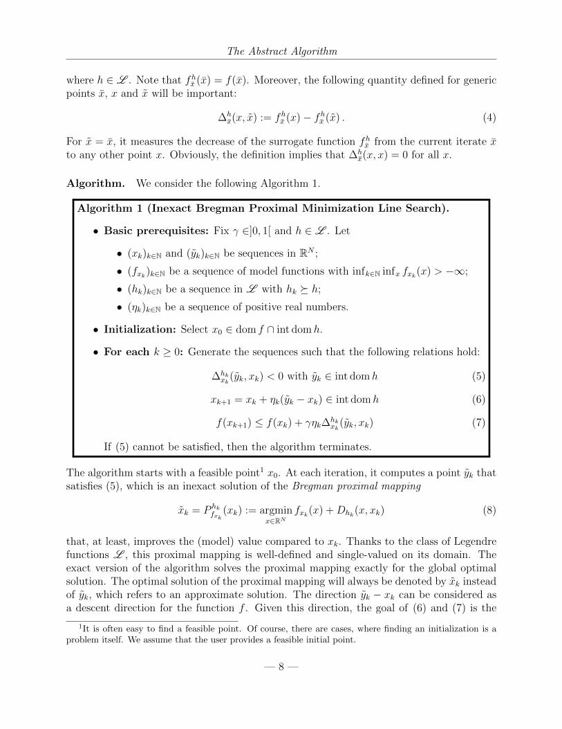
Algorithm. We consider the following Algorithm 1.
Algorithm 1 (Inexact Bregman Proximal Minimization Line Search).
• Basic prerequisites: Fix γ ∈]0, 1[ and h ∈ L . Let
• (xk)k∈N and (yk)k∈N be sequences in RN ;
• (fxk)k∈N be a sequence of model functions with infk∈N infx fxk(x) > −∞;
• (hk)k∈N be a sequence in L with hk h;
• (ηk)k∈N be a sequence of positive real numbers.
• Initialization: Select x0 ∈ dom f ∩ int domh.
• For each k ≥ 0: Generate the sequences such that the following relations hold:
∆hkxk
(yk, xk) < 0 with yk ∈ int domh (5)
xk+1 = xk + ηk(yk − xk) ∈ int domh (6)
f(xk+1) ≤ f(xk) + γηk∆hkxk
(yk, xk) (7)
If (5) cannot be satisfied, then the algorithm terminates.
The algorithm starts with a feasible point1 x0. At each iteration, it computes a point yk thatsatisfies (5), which is an inexact solution of the Bregman proximal mapping
xk = P hkfxk
(xk) := argminx∈RN
fxk(x) +Dhk(x, xk) (8)
that, at least, improves the (model) value compared to xk. Thanks to the class of Legendrefunctions L , this proximal mapping is well-defined and single-valued on its domain. Theexact version of the algorithm solves the proximal mapping exactly for the global optimalsolution. The optimal solution of the proximal mapping will always be denoted by xk insteadof yk, which refers to an approximate solution. The direction yk − xk can be considered asa descent direction for the function f . Given this direction, the goal of (6) and (7) is the
1It is often easy to find a feasible point. Of course, there are cases, where finding an initialization is aproblem itself. We assume that the user provides a feasible initial point.
— 8 —

The Abstract Algorithm
estimation of a step size ηk (by line search, cf. Algorithm 2) that reduces the value of theobjective function. In case that the proximal mapping has a solution but the first relation(5) can only be satisfied with equality, we will see that xk = yk must be a stationary pointof the objective, hence, the algorithm terminates.
Remark 12. Instead of performing backtracking on the objective values as in Algorithm 1,backtracking on the scaling of the Bregman distance in (5) is also possible. For a specialmodel function, this leads to ProxDescent [25, 20] (with Euclidean proximity function). If ascaled version of (5) yields a descent on f , we can set ηk = 1, and accept this point. However,this can be expensive when the proximal subproblem in (5) is hard to solve, since each trialstep requires to solve the subproblem. In order to break the backtracking, the new objectivevalue must be computed anyway. Therefore, a computational advantage of the line search(6) and (7) is to be expected (cf. Section 6.1).
Algorithm 2 (Line Search for Algorithm 1).
• Basic prerequisites: Fix δ, γ ∈]0, 1[, η > 0, and k ∈ N.
• Input: Current iterates xk ∈ int domh and yk satisfy (5).
• Solve: Find the smallest j ∈ N such that ηj := ηδj satisfies (6) and (7).
• Return: Set the feasible step size ηk for iteration k to ηj.
Algorithm 1–2 is well defined as the following lemmas show.
Lemma 13 (Well-definedness). Let ω in (3) be a growth function. Algorithm 1 is well-defined, i.e., for all k ∈ N, the following holds:
(i) there exists yk that satisfies (5) or xk = xk and the algorithm terminates;
(ii) xk ∈ dom f ∩ int domh; and
(iii) there exists ηk that satisfies (6) and (7).
Proof. (i) For xk ∈ int domh, Lemma 10 shows that P hkfxk
maps to int domhk ∩ dom fxk ⊂int domh ∩ dom f and is single-valued. Thus, for example, yk = xk satisfies (5). Otherwise,xk = xk, which shows (i). (ii) Since x0 ∈ dom f ∩ int domh and f(xk+1) ≤ f(xk) by (7)it holds that xk ∈ dom f for all k. Since xk ∈ int domh and yk ∈ domh, for small ηk alsoxk+1 ∈ int domh, hence xk+1 ∈ dom f ∩ int domh. Inductively, we conclude the statement.(iii) This will be shown in Lemma 14.
Lemma 14 (Finite termination of Algorithm 2). Consider Algorithm 1 and fix k ∈ N.Let ω in (3) be a growth function. Let δ, γ ∈]0, 1[, η > 0, h := hk, and x := xk, y := yk besuch that ∆h
x(y, x) < 0. Then, there exists j ∈ N such that ηj := ηδj satisfies
f(x+ ηj(y − x)) ≤ f(x) + γηj∆hx(y, x) .
— 9 —

Finite Time Convergence Analysis
Proof. This result is proved by contradiction. Define v := y − x. By our assumption in (3),we observe that
f(x+ ηjv)− f(x) ≤ fx(x+ ηjv)− f(x) + o(ηj) . (9)
Using Jensen’s inequality for the convex function fx provides:
fx(x+ ηjv)− fx(x) ≤ ηjfx(x+ v) + (1− ηj)fx(x)− fx(x) = ηj ·(fx(x+ v)− fx(x)
). (10)
Now, suppose γ∆hx(y, x) < 1
ηj(f(x + ηjv) − f(x)) holds for any j ∈ N. Then, using (9) and
(10), we conclude the following:
γ∆hx(y, x) < fx(x+ v)− fx(x) + o(ηj)/ηj
≤ fx(x+ v)− fx(x) +Dh(y, x) + o(ηj)/ηj
= (f hx (y)− f hx (x)) + o(ηj)/ηj = ∆hx(y, x) + o(ηj)/ηj ,
which for j →∞ yields the desired contradiction, since γ ∈]0, 1[ and ∆hx(y, x) < 0.
4.2 Finite Time Convergence Analysis
First, we study the case when the algorithm terminates after a finite number of iterations,i.e., there exists k0 ∈ N such that (5) cannot be satisfied. Then, the point yk0 is a global
minimizer of fhk0xk0
and ∆hk0xk0
(yk0 , xk0) = 0. Moreover, the point xk0 turns out to be a stationarypoint of f .
Lemma 15. For x ∈ dom f and a model fx that satisfies (3), where ω is a growth function,the following holds:
|∇fx|(x) = |∇f |(x) .
Proof. Since ω(0) = 0, we have from (3) that fx(x) = f(x). This, together with sub-additivity of [·]+, entails
[fx(x)− fx(x)]+|x− x|
≤ [f(x)− f(x)]+ + [f(x)− fx(x)]+|x− x|
≤ [f(x)− f(x)]+|x− x|
+|f(x)− fx(x)||x− x|
≤ [f(x)− f(x)]+|x− x|
+ω(|x− x|)|x− x|
Passing to the lim sup on both sides and using that ω ∈ o(t), we get
|∇fx|(x) ≤ |∇f |(x).
Arguing similarly but now starting with |∇f |(x), we get the reverse inequality, which in turnshows the claimed equality.
Proposition 16 (Stationarity for finite time termination). Consider the setting ofAlgorithm 1. Let ω in (3) be a growth function. Let k0 ∈ N be fixed, and set x = yk0 ,x = xk0 , h = hk0 , and x, x ∈ dom f ∩ int domh. If ∆h
x(x, x) ≥ 0, then x = x, ∆hx(x, x) = 0,
and |∇f |(x) = 0, i.e. x is a stationary point of f .
— 10 —

Asymptotic Convergence Analysis
Proof. Since x is the unique solution of the proximal mapping, obviously ∆hx(x, x) = 0 and
x = x. Moreover, x is the minimizer of f hx , i.e. we have
0 = |∇f hx |(x) = |∇f hx |(x) = lim supx→xx 6=x
[fx(x)− fx(x)−Dh(x, x)]+|x− x|
= |∇fx|(x) = |∇f |(x) ,
where we used that h is Frechet differentiable at x and Lemma 15.
4.3 Asymptotic Convergence Analysis
We have established stationarity of the algorithm’s output, when it terminates after a finitenumber of iterations. Therefore, without loss of generality, we now focus on the case where(5) can be satisfied for all k ∈ N. We need to make the following assumptions.
Assumption 1. The sequence (yk)k∈N satisfies fhkxk (yk) ≤ inf fhkxk + εk for some εk → 0.
Remark 17. Assumption 1 states that asymptotically (for k →∞) the Bregman proximalmapping (8) must be solved accurately. In order to obtain stationarity of a limit point,Assumption 1 is necessary, as shown by Bonettini et al. [11, after Theorem 4.1] for a specialsetting of model functions.
Assumption 2. Let h ∈ L . For every bounded sequences (xk)k∈N and (xk)k∈N in int domh,and (hk)k∈N such that hk h, it is assumed that:
xk − xk → 0 ⇔ Dhk(xk, xk)→ 0 .
Remark 18. (i) Assumption 2 states that (asymptotically) a vanishing Bregman distancereflects a vanishing Euclidean distance. This is a natural assumption and satisfied, e.g.,by most entropies such as Boltzmann–Shannon, Fermi–Dirac, and Burg entropy.
(ii) The equivalence in Assumption 2 is satisfied, for example, when there exists c ∈ Rsuch that c h hk holds for all k ∈ N and the following holds:
xk − xk → 0 ⇔ Dh(xk, xk)→ 0 .
Proposition 19 (Convergence of objective values). Consider the setting of Algorithm 1.Let ω in (3) be a growth function. The sequence of objective values (f(xk))k∈N is non-increasing and converging to some f ∗ ≥ f > −∞.
Proof. This statement is a consequence of (7) and (5), and the lower-boundedness of f .
Asymptotically, under some condition on the step size, the improvement of the modelobjective value between yk and xk must tend to zero. Since we do not assume that the stepsizes ηk are bounded away from zero, this is a non-trivial result.
— 11 —

Asymptotic Convergence Analysis
Proposition 20 (Vanishing model improvement). Consider the setting of Algorithm 1.Let ω in (3) be a growth function. Suppose, either2 infk ηk > 0 or ηk is selected by the LineSearch Algorithm 2. Then,
∞∑k=0
ηk(−∆hkxk
(yk, xk)) < +∞ and ∆hkxk
(yk, xk)→ 0 as k →∞.
Proof. The first part follows from rearranging (7), and summing both sides for k = 0, . . . , n:
γn∑k=0
ηk(−∆hkxk
(yk, xk)) ≤n∑k=0
(f(xk)− f(xk+1)) = f(x0)− f(xn+1) ≤ f(x0)− f ∗ .
In the remainder of the proof, we show that ∆hkxk
(yk, xk) → 0, which is not obvious unlessinfk ηk > 0. The model improvement is bounded. Boundedness from above is satisfied byconstruction of the sequence (yk)k∈N. Boundedness from below follows from the followingobservation and the uniform boundedness of the model functions from below:
∆hkxk
(yk, xk) = fhkxk (yk)− fhkxk (xk) ≥ fhkxk (xk)− f(xk) ≥ fxk(xk)− f(x0) .
Therefore, there exists K ⊂ N such that the subsequence ∆hkxk
(yk, xk) converges to some ∆∗
as kK→ ∞. Suppose ∆∗ < 0. Then, the first part of the statement implies that the step
size sequence must tend to zero, i.e., ηk → 0 for kK→ ∞. For k ∈ K sufficiently large, the
line search procedure in Algorithm 2 reduces the step length from ηk/δ to ηk. (Note thatηk can be assumed to be the “first” step length that achieves a reduction in (7)). Beforemultiplying with δ, no descent of (7) was observed, i.e.,
(ηk/δ)γ∆hkxk
(yk, xk) < f(xk + (ηk/δ)vk)− f(xk) ,
where vk = yk − xk. Using (9) and (10), we can make the same observation as in the proofof Lemma 14:
γ∆hkxk
(yk, xk) < fxk(xk + v)− fxk(xk) + o(ηk/δ)/(ηk/δ)
≤ fxk(xk + v)− fxk(xk) +Dhk(yk, xk) + o(ηk)/ηk
= (fhkxk (yk)− fhkxk (xk)) + o(ηk)/ηk
= ∆hkxk
(yk, xk) + o(ηk)/ηk ,
which for ηk → 0 yields a contradiction, since γ ∈]0, 1[ and ∆hkxk
(yk, xk) < 0. Therefore, anycluster point ∆∗ of (∆hk
xk(yk, xk))k∈K must be 0, which concludes the proof.
4.3.1 Asymptotic Stationarity with a Growth Function
In order to establish stationarity of limit points generated by Algorithm 1 additional assump-tions are required. We consider three different settings for the model assumption (3): ω inthe model assumption (3) is a growth function (this section), ω is a proper growth function(Section 4.3.2), and ω is global growth function of the form ω = Dh (Section 4.3.3).
2Note that infk ηk > 0 is equivalent to lim infk ηk > 0 as we assume ηk > 0 for all k ∈ N.
— 12 —
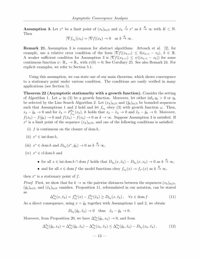
Asymptotic Convergence Analysis
Assumption 3. Let x∗ be a limit point of (xk)k∈N and xkf→ x∗ as k
K→ ∞ with K ⊂ N.Then
|∇fxk |(xk) = |∇f |(xk)→ 0 as kK→∞ .
Remark 21. Assumption 3 is common for abstract algorithms. Attouch et al. [2], forexample, use a relative error condition of the form |∇f |(xk+1) ≤ b|xk+1 − xk|, b ∈ R.A weaker sufficient condition for Assumption 3 is |∇f |(xk+1) ≤ ψ(|xk+1 − xk|) for somecontinuous function ψ : R+ → R+ with ψ(0) = 0; See Corollary 25. See also Remark 24. Forexplicit examples, we refer to Section 5.1.
Using this assumption, we can state one of our main theorems, which shows convergenceto a stationary point under various condition. The conditions are easily verified in manyapplications (see Section 5).
Theorem 22 (Asymptotic stationarity with a growth function). Consider the settingof Algorithm 1. Let ω in (3) be a growth function. Moreover, let either infk ηk > 0 or ηkbe selected by the Line Search Algorithm 2. Let (xk)k∈N and (yk)k∈N be bounded sequencessuch that Assumptions 1 and 2 hold and let fxk obey (3) with growth function ω. Then,xk − yk → 0 and for xk = P hk
fxk(xk), it holds that xk − xk → 0 and xk − yk → 0. Moreover,
f(xk)− f(yk)→ 0 and f(xk)− f(xk)→ 0 as k →∞. Suppose Assumption 3 is satisfied. Ifx∗ is a limit point of the sequence (xk)k∈N, and one of the following conditions is satisfied:
(i) f is continuous on the closure of domh,
(ii) x∗ ∈ int domh,
(iii) x∗ ∈ domh and Dhk(x∗, yk)→ 0 as kK→∞,
(iv) x∗ ∈ cl domh and
• for all x ∈ int domh ∩ dom f holds that Dhk(x, xk)−Dhk(x, xk)→ 0 as kK→∞,
• and for all x ∈ dom f the model functions obey fxk(x)→ fx∗(x) as kK→∞,
then x∗ is a stationary point of f .
Proof. First, we show that for k →∞ the pairwise distances between the sequences (xk)k∈N,(yk)k∈N, and (xk)k∈N vanishes. Proposition 11, reformulated in our notation, can be statedas
∆hkxk
(x, xk) = fhkxk (x)− fhkxk (xk) ≥ Dhk(x, xk) , ∀x ∈ dom f . (11)
As a direct consequence, using x = yk together with Assumptions 1 and 2, we obtain
Dhk(yk, xk)→ 0 thus xk − yk → 0 .
Moreover, from Proposition 20, we have ∆hkxk
(yk, xk)→ 0, and from
∆hkxk
(yk, xk) = ∆hkxk
(yk, xk)−∆hkxk
(xk, xk) ≤ ∆hkxk
(yk, xk)−Dhk(xk, xk) , (12)
— 13 —

Asymptotic Convergence Analysis
and Assumptions 1 and 2, we conclude that xk − xk → 0, hence also xk − yk → 0.
The next step is to show that f(xk) − f(yk) → 0 as k → ∞. This follows from thefollowing estimation:
|f(xk)− f(yk)| ≤ |fxk(xk)− fxk(yk)|+ ω(|yk − xk|)≤ |fhkxk (xk)− fhkxk (yk)|+Dhk(yk, xk) + ω(|yk − xk|)= |∆hk
xk(xk, yk)|+Dhk(yk, xk) + ω(|yk − xk|) ,
(13)
where the right hand side vanishes for k → ∞. Analogously, we can show that f(xk) −f(xk)→ 0 as k →∞.
Let x∗ be the limit point of the subsequence (xk)k∈K for some K ⊂ N. The remainderof the proof shows that f(yk) → f(x∗) as k → ∞. Then f(xk) − f(yk) → 0 implies that
xkf→ x∗ as k
K→ ∞, and by Assumption 3, the slope vanishes, hence the limiting slope|∇f |(x∗) at x∗ also vanishes, which concludes the proof.
(i) implies f(yk)→ f(x∗) as k →∞ by definition. For (ii) and (iii), we make the followingobservation:
f(yk)−ω(|yk−xk|) ≤ fhkxk (yk) = fhkxk (xk)+(fhkxk (yk)−fhkxk (xk)) ≤ fhkxk (x∗)+∆hkxk
(yk, xk) , (14)
where xk = P hkfxk
(xk). Taking “lim supkK→∞
” on both sides, Dhk(x∗, xk) → 0 (Assump-
tion 2 for (ii) or the assumption in (iii)), and ∆hkxk
(yk, xk) → 0 (Assumption 1) shows thatlim sup
kK→∞
f(yk) ≤ f(x∗). Since f is closed, f(yk)→ f(x∗) holds.
We consider (iv). For all x ∈ int domh∩ dom f , we have (11) or, reformulated, fhkxk (x)−Dhk(x, xk) ≥ fhkxk (xk), which implies the following:
fxk(x) +Dhk(x, xk)−Dhk(x, xk)−Dhk(xk, xk) ≥ f(xk)− ω(|xk − xk|) .
Note that for any x the limits for kK→∞ on the left hand side exist. In particular, we have
Dhk(x, xk)−Dhk(x, xk)−Dhk(xk, xk)→ 0 as kK→∞ ,
by the assumption in (iv), and Assumption 2 together with xk − xk → 0. The limit offxk(x) exists by assumption and coincides with fx∗(x). Choosing a sequence (zk)k∈N in
int domh ∩ dom f with zk → x∗ as kK→∞, in the limit, we obtain
f(x∗) ≥ limkK→∞
f(xk) =: f ∗ ,
since fx∗(zk) → fx∗(x∗) = f(x∗) for zk → x∗ as kK→ ∞. Invoking that f is closed, we
conclude the f -attentive convergence f ∗ = lim infk→∞ f(xk) ≥ f(x∗) ≥ f ∗.
— 14 —

Asymptotic Convergence Analysis
Remark 23. Existence of a limit point x∗ is guaranteed by assuming that (xk)k∈N is bounded.Alternatively, we could require that f is coercive (i.e. f(xk) → ∞ for |xk| → ∞), whichimplies boundedness of the lower level sets of f , hence by Proposition 19 the boundednessof (xk)k∈N.
Remark 24. From Theorem 22, clearly, also ykf→ x∗ and xk
f→ x∗ as kK→ ∞ holds.
Therefore, Assumption 3 could also be stated as the requirement
|∇f |(xk)→ 0 or |∇f |(yk)→ 0 as kK→∞ ,
in order to conclude that limit points of (xk)k∈N are stationary points.
As a simple corollary of this theorem, we replace Assumption 3 with the relative errorcondition mentioned in Remark 21.
Corollary 25 (Asymptotic stationarity with a growth function). Consider the settingof Algorithm 1. Let ω in (3) be a growth function. Moreover, let either infk ηk > 0 or ηkbe selected by the Line Search Algorithm 2. Let (xk)k∈N and (yk)k∈N be bounded sequencessuch that Assumptions 1 and 2 hold and let fxk obey (3) with growth function ω. Supposethere exists a continuous function ψ : R+ → R+ with ψ(0) = 0 such that |∇f |(xk+1) ≤ψ(|xk+1 − xk|) is satisfied. If x∗ is a limit point of the sequence (xk)k∈N and one of theconditions (i)–(iv) in Theorem 22 is satisfied, then x∗ is a stationary point of f .
Proof. Theorem 22 shows that yk − xk → 0, thus, infk ηk > 0 implies xk+1 − xk → 0 by (6).Therefore, the relation |∇f |(xk+1) ≤ ψ(|xk+1−xk|) shows that Assumption 3 is automaticallysatisfied and we can apply Theorem 22 to deduce the statement.
Some more results on the limit point set. In Theorem 22 we have shown that limitpoints of the sequence (xk)k∈N generated by Algorithm 1 are stationary, and in fact the se-quence f -converges to its limit points. The following proposition shows some more propertiesof the set of limit points of (xk)k∈N. This is a well-known result [10, Lem. 5] that followsfrom xk+1 − xk → 0 as k →∞.
Proposition 26. Consider the setting of Algorithm 1. Let ω in (3) be a growth function andinfk ηk > 0. Let (xk)k∈N and (yk)k∈N be bounded sequences such that Assumptions 1, 2 and 3hold. Suppose one of the conditions (i)–(iv) in Theorem 22 is satisfied for each limit point
of (xk)k∈N. Then, the set S :=x∗ ∈ RN | ∃K ⊂ N : xk → x∗ as k
K→∞
of limit points of
(xk)k∈N is connected, each point x∗ ∈ S is stationary for f , and f is constant on S.
Proof. Theorem 22 shows that yk − xk → 0. Thus, boundedness of ηk away from 0 impliesxk+1 − xk → 0 by (6). Now, the statement follows from [10, Lem. 5] and Theorem 22.
4.3.2 Asymptotic Stationarity with a Proper Growth Function
Our proof of stationarity of limit points generated by Algorithm 1 under the assumptionof a proper growth function ω in (3) relies on an adaptation of a recently proved result by
— 15 —

Asymptotic Convergence Analysis
Drusvyatskiy et al. [19, Corollary 5.3], which is stated in Lemma 27 before the main theoremof this subsection. The credits for this lemma should go to [19].
Lemma 27 (Perturbation result under approximate optimality). Let f : RN → R bea proper closed function. Consider bounded sequences (xk)k∈N and (yk)k∈N with xk− yk → 0for k →∞, and model functions fhkxk according to (3) with proper growth functions. SupposeAssumption 1 and 2 hold. If (x∗, f(x∗)) is a limit point of (xk, f(xk))k∈N, then x∗ is stationaryfor f .
Proof. Recall εk from Assumption 1. Theorem 5.1 from [19] guarantees, for each k and anyρk > 0, the existence of points yk and zk such that the following hold:
(i) (point proximity)
|yk − zk| ≤εkρk
and |zk − yk| ≤ 2 · ω(|zk − xk|)ω′+(|zk − xk|)
,
under the convention 00
= 0 ,
(ii) (value proximity) f(yk) ≤ f(yk) + 2ω(|zk − xk|) + ω(|yk − xk|), and
(iii) (near-stationarity) |∇f |(y) ≤ ρk + ω′+(|zk − xk|) + ω′+(|yk − xk|),
Setting ρk =√εk, using εk → 0 and the point proximity, shows that |yk−zk| → 0. Moreover
|zk − xk| ≤ |zk − yk| + |yk − xk| → 0, which implies that |zk − yk| → 0. Now, we fix a
convergent subsequence (xk, f(xk)) → (x∗, f(x∗)) as kK→ ∞ for some K ⊂ N. Using (11),
we observe xk − yk → 0, hence xk − xk → 0. From Proposition 20 and Assumption 1, weconclude that ∆hk
xk(yk, xk) → 0, and, therefore f(xk) − f(yk) → 0 using (13). Consider the
value proximity. Combined with the lower semi-continuity of f , it yields
f(x∗) ≤ lim infkK→∞
f(yk) ≤ lim supkK→∞
f(yk) ≤ lim supkK→∞
f(yk) ≤ f(x∗) ,
hence (yk, f(yk)) → (x∗, f(x∗)) as kK→ ∞. Near-stationarity implies that |∇f |(yk) → 0,
which proves that |∇f |(x∗) = 0, hence x∗ is a stationary point.
Remark 28. The setting in [19, Corollary 5.3] is recovered when (xk)k∈N is given by xk+1 =yk.
Theorem 29 (Asymptotic stationarity with a proper growth function). Considerthe setting of Algorithm 1. Let ω in (3) be a proper growth function. Moreover, let eitherinfk ηk > 0 or ηk be selected by the Line Search Algorithm 2. Let (xk)k∈N and (yk)k∈N bebounded sequences such that Assumptions 1 and 2 hold. If x∗ is a limit point of the sequencexk and one of the conditions (i)–(iv) in Theorem 22 is satisfied, then x∗ is a stationary pointof f .
— 16 —

Asymptotic Convergence Analysis
Proof. Propositions 19 and 20, and the proof of f -attentive convergence from Theorem 22only rely on a growth function. Instead of assuming that the slope vanishes, here we applyLemma 27 to conclude stationarity of the limit points.
Of course, Proposition 26 can also be stated in the context here.
4.3.3 Asymptotic Analysis with a Global Growth Function
Suppose, for x ∈ int domh for some h ∈ L , the model error can be estimated as follows:
|f(x)− fx(x)| ≤ LDh(x, x) ∀x . (15)
Since h is Frechet differentiable on int domh, the right hand side is bounded by a growthfunction. Without loss of generality, we restrict ourselves to a fixed function h ∈ L (this sec-tion analyses a single iteration). In order to reveal similarities to well-known step size rules,we scale h in the definition of fhx to Dh/α = 1
αDh with α > 0 instead of Dh. Here, decreasing
objective values can be assured without the line search procedure (see Proposition 30), i.e.,ηk = 1 is always feasible.
In order to obtain the result of stationarity of limit points (Theorem 22 or 29), we caneither verify by hand that Assumption 3 holds or we need to assume that Dh(x, x) is boundedby a proper growth function.
Proposition 30. Consider the setting of Algorithm 1 and let (15) be satisfied.
(i) For points y that satisfy ∆hx(y, x) < 0,
1− αLα
Dh(y, x) ≤ f(x)− f(y)
holds, where the left-hand-side is strictly larger than 0 for α ∈]0, 1/L[.
(ii) For points x = P hfx
(x), the following descent property holds:
1 + ρ− αLα
Dh(x, x) ≤ f(x)− f(x) ,
where the left-hand-side is strictly larger than 0 for α ∈]0, (1 + ρ)/L[, and ρ is the
Bregman symmetry factor defined by ρ := infDh(x,x)Dh(x,x)
|x, x ∈ int domh , x 6= x
; (see
[6]).
Proof. The following relations hold:
∆hx(y, x) ≤ 0 ⇔ fhx (y) ≤ fhx (x) ⇔ fx(y) +
1
αDh(y, x) ≤ fx(x) = f(x) . (16)
Bounding the left hand side of the last expression using (15), we obtain
f(y)− LDh(y, x) +1
αDh(y, x) ≤ f(x) , (17)
— 17 —

A Remark on Convex Optimization
which proves part (i). Part (ii) follows analogously. However, thanks to the three pointinequality from Proposition 11 and optimality of x the rightmost inequality of (16) improvesto
fx(x) +1
αDh(x, x) +
1
αDh(x, x) ≤ fx(x) = f(x) ,
and the statement follows.
4.4 A Remark on Convex Optimization
In this section, let f be convex, and consider the following global model assumption
0 ≤ f(x)− fx(x) ≤ LDh(x, x) . (18)
We establish a convergence rate of O(1/k) for Algorithm 1 with ηk ≡ 1. For Forward–Backward Splitting, this has been shown by Bauschke et al. [6]. We only require fx to be amodel w.r.t. (18).
Proposition 31. Consider Algorithm 1 with ηk ≡ 1 and model functions that obey (18).
For xk+1 = Ph/αfxk
(xk) and α = 1L
, the following rate of convergence on the objective values
holds:
f(xk+1)− f(x) ≤ LDh(x∗, x0)
2k(= O(1/k)) .
Proof. The three point inequality in Proposition 11 combined with the model assumption(18) yields the following inequality:
f(x) +1− αLα
Dh(x, x) +1
αDh(x, x) ≤ f(x) +
1
αDh(x, x)
for all x. Restricting to 0 < α ≤ 1L
, we obtain
f(x)− f(x) ≤ 1
α(Dh(x, x)−Dh(x, x)) . (19)
Let x∗ be a minimizer of f . We make the following choices:
x = x∗ , x = xk+1 , and x = xk .
Summing both sides up to iteration k and the descent property yield the convergence rate:
f(xk+1)− f(x) ≤ Dh(x∗, x0)
2αk
α= 1L=LDh(x
∗, x0)
2k. (20)
Example 32. This section goes beyond the Forward–Backward Splitting setting, e.g., wemay specialize Example 35 to convex problems of the form minx g(F (x)), for instance, usingF (x) = (f1(x), f2(x)) and g(z1, z2) = maxz1, z2.
— 18 —

Examples
5 Examples
We discuss several classes of problems that can be solved using our framework. To apply Al-gorithm 1, in Section 5.1, we define a suitable model and mention the associated algorithmicstep that arises from exactly minimizing the sum of the model and an Euclidean proximitymeasure. However our algorithm allows for inexact solutions and very flexible (also itera-tion dependent) Bregman proximity functions. Examples are provided in Section 5.2. Forbrevity, we define the symbols Γ0 for the set of proper, closed, convex functions and C1 forthe set of continuously differentiable functions.
5.1 Examples of Model Functions
Example 33 (Forward–Backward Splitting). Problems of the form
f = f0 + f1 with f0 ∈ Γ0 and f1 ∈ C1
can be modeled byfx(x) = f0(x) + f1(x) + 〈x− x,∇f1(x)〉 .
This model is associated with Forward–Backward Splitting (FBS). We assume that one ofthe following error models is satisfied:
|f(x)−fx(x)| = |f1(x)−f1(x)−〈x− x,∇f1(x)〉 | ≤
L2|x− x|2 , if ∇f1 is L-Lipschitz ;∫ 1
0ϕ(t|x−x|)
tdt ,
if ∇f1 is ψ-uniformcontinuous ;
ω(|x− x|) , otherwise ,
which is the linearization error of the smooth part f1. The first case obeys a global (proper)growth function, derived from the common Descent Lemma. The second case is the general-ization to a ψ-uniformly continuous gradient with ϕ(s) = sψ(s) as in Lemma 4. The bound∫ 1
0ϕ(t|x−x|)
tdt is a growth function but not necessarily a proper growth function. The third
case is the most general and assumes that the error obeys a growth function. In any case,the model satisfies the model consistency required in Theorem 22(iv). For any x ∈ dom fand x→ x∗,
|f0(x) + f1(x) + 〈x− x,∇f1(x)〉 − (f0(x) + f1(x∗) + 〈x− x∗,∇f1(x∗)〉)| → 0
holds, thanks to the continuous differentiability of f1 and continuity of the inner product.
In order to verify Assumption 3, we make use of Remark 24 and show that |∇f |(xk)→ 0
as kK→∞ where K ⊂ N is such that xk
K→ x∗. Note that xk satisfies the following relation:
0 ∈ ∂f0(xk) +∇f1(xk) +∇hk(xk)−∇hk(xk)⇒ ∇f1(xk)−∇f1(xk) +∇hk(xk)−∇hk(xk) ∈ ∂f0(xk) +∇f1(xk) = ∂f(xk)
— 19 —
Examples of Model Functions
Moreover, we know that xk − xk → 0 as kK→ ∞. Since ∇f1 is continuous, if |∇hk(xk) −
∇hk(xk)| → 0 for kK→ ∞, then Assumption 3/Remark 24 is satisfied. The condition
|∇hk(xk) − ∇hk(xk)| → 0 is naturally fulfilled by many Legendre functions, e.g., if ∇hk isψ-uniformly continuous (uniformly in k) with α > 0 or uniformly continuous (independentof k) on bounded sets or continuous at x∗ (uniformly w.r.t. k), and will be discussed in moredetail in Section 5.2.
Example 34 (Variable metric FBS). We consider an extension of Examples 33. Analternative feasible model for a twice continuously differentiable function f1 is the following:
fx(x) = f0(x) + f1(x) + 〈x− x,∇f1(x)〉+1
2〈x− x, B(x− x)〉 ,
where B := [∇2f1(x)]+ is a positive definite approximation to ∇2f1(x), which leads toa Hessian driven variable metric FBS. It is easy to see that the model error satisfies thegrowth function ω(s). Again, Theorem 22(iv) obviously holds and the same conclusionsabout Assumption 3 can be made as in Example 33.
Example 35 (ProxDescent). Problems of the form
f0 + g F with f0 ∈ Γ0 , F ∈ C1 , and g ∈ Γ0 finite-valued ,
which often arise from non-linear inverse problems, can be approached by the model function
fx(x) = f0(x) + g(F (x) +DF (x)(x− x)) ,
where DF (x) is the Jacobian matrix of F at x. The associated algorithm is connected toProxDescent [25, 20]. If g is a quadratic function, the algorithm reduces to the Levenberg–Marquardt algorithm [27]. The error model can be computed as follows:
|f(x)− fx(x)| = |g(F (x))− g(F (x) +DF (x)(x− x))|≤ `|F (x)− F (x)−DF (x)(x− x)|
≤
`L2|x− x|2 , if DF is L-Lipschitz and g is `-Lipschitz ;
`∫ 1
0ϕ(t|x−x|)
tdt , if DF is ψ-uniform continuous and g is `-Lipschitz ;
ω(|x− x|) , otherwise ,
(21)
where ` is the (possibly local) Lipschitz constant of g around F (x). Since g is convex andfinite-valued, it is always locally Lipschitz continuous. Since F is continuously differentiable,for x sufficiently close to x, both F (x) and F (x)+DF (x)(x−x) lie in a neighborhood of F (x)where the local Lipschitz constant ` of g is valid, which shows the first inequality in (21).The last line in (21) assumes that, either the linearization error of F obeys a global proper
growth function, the specific growth function∫ 1
0ϕ(t|x−x|)
tdt, or it obeys a growth function
— 20 —

Examples of Model Functions
ω(s). With a similar reasoning, we can show that Theorem 22(iv) is satisfied.
We consider Assumption 3 (see also Remark 24). Let xk → x∗ as kK→ ∞ for K ⊂ N
and xk − xk → 0. Since g is finite-valued, using [7, Corollary 16.38] (sum-rule for thesubdifferential), and [36, Theorem 10.6], we observe that
0 ∈ ∂f0(xk) +DF (xk)∗∂g(F (xk) +DF (xk)(xk − xk)) +∇hk(xk)−∇hk(xk) , (22)
where DF (xk)∗ denotes the adjoint of DF (xk). We can assume that, for k large enough,
F (xk)+DF (xk)(xk−xk) and F (xk) lie a neighborhood of F (x∗) on which g has the Lipschitzconstant ` > 0. By [36, Theorem 9.13], ∂g is locally bounded around F (x∗), i.e. there existsa compact set G such that ∂g(z) ⊂ G for all z in a neighborhood of F (x∗). We concludethat
supv∈∂g(F (xk)+DF (xk)(xk−xk))
w∈∂g(F (xk))
|DF (xk)∗v −DF (xk)
∗w| ≤ supv,w∈G
|DF (xk)∗v −DF (xk)
∗w| → 0
for kK→ ∞ since DF (xk) → DF (x∗) and DF (xk) → DF (x∗). Again assuming that
∇hk(xk) − ∇hk(xk) → 0 we conclude that the outer set-limit of the right hand side of
(22) is included in ∂f(xk) and, therefore, the slope |∇f |(xk) vanishes for kK→∞.
Example 36. Problems of the form
f0+gF with f0 ∈ Γ0 , g ∈ C1 ,∇gi ≥ 0 , and F = (F1, . . . , FM) is Lipschitz with Fi ∈ Γ0
can be modeled by
fx(x) = f0(x) + g(F (x)) + 〈F (x)− F (x),∇g(F (x))〉 .
Such problems appear for example in non-convex regularized imaging problems in the contextof iteratively reweighted algorithms [33]. For the error of this model function, we observethe following:
|f(x)− fx(x)| = |g(F (x))− (g(F (x)) + 〈F (x)− F (x),∇g(F (x))〉)|
≤
`2|F (x)− F (x)|2 , if ∇g is `-Lipschitz ;∫ 1
0ϕ(t|F (x)−F (x)|)
tdt , if ∇g is ψ-uniform continuous ;
ω(|F (x)− F (x)|) , otherwise ;
≤
`L2
2|x− x|2 , if ∇g is `-Lipschitz and F is L-Lipschitz ;∫ 1
0ϕ(tL|x−x|))
tdt ,
if ∇g is ψ-uniform continuous andF is L-Lipschitz ;
ω(c|x− x|) , otherwise ,
which shows the same growth functions are obeyed as in Example 33 and 35. The explana-tion for the validity of the reformulations are analogue to those of Example 35. It is easy to
— 21 —

Examples of Bregman functions
see that Theorem 22(iv) holds.
We consider Assumption 3/Remark 24. Let xk → x∗ as kK→ ∞ for K ⊂ N and xk −
xk → 0. Since g is continuously differentiable, the sum-formula for the subdifferential holds.Moreover, we can apply [36, Corollary 10.09] (addition of functions) to see that xk satisfiesthe following relation:
0 ∈ ∂f0(xk) +M∑i=1
∂Fi(xk)(∇g(F (xk)))i +∇hk(xk)−∇hk(xk) ,
Note that by [36, Theorem 10.49] the subdifferential of gF at xk is∑M
i=1 ∂Fi(xk)(∇g(F (xk)))i.As in Example 35, using the Lipschitz continuity of F , hence local boundedness of ∂F , andusing the continuous differentiability of g, the sequence of sets
∑Mi=1 ∂Fi(xk)(∇g(F (xk)))i −
∂Fi(xk)(∇g(F (xk)))i vanishes for kK→ ∞, which implies that the slope |∇f |(xk) vanishes
for kK→∞.
Example 37 (Problem adaptive model function). Our framework allows for a problemspecific adaptation using a combination of Examples 33, 34, 35, and 36. Consider thefollowing objective function3 f : RN × R2 → R with a ∈ RN and b ∈ R:
f(x, z) = f1(z) + δ[−1,1]2(z) + f2(x) with
f1 ∈ C2(R2) is strongly convex ;
f2(x) := max(〈a, x〉 − b)2, 1− exp(−|x|) .
We define our model function as: f(x,z)(x, z) = f1(z; z) + δ[−1,1](z) + f2(x; x) with
f1(z; z) := f1(z) + 〈∇f1(z), z − z〉+1
2
⟨z − z,∇2f1(z)(z − z)
⟩;
f2(x; x) := max(〈ai, x〉 − bi)2, 1 + exp(−|x|)(|x| − |x| − 1) .
The strong convexity of f1 allows for a convex second order approximation with positivedefinite Hessian. We linearize only the second component of the “max” (w.r.t. |x|) in f2 toobtain a convex approximation that is as close as possible to original function f2.
As ∇f1 is Lipschitz continuous on the compact set [0, 1]2, the growth function w.r.t. z isof the form L|z − z|2. Moreover, using 1-Lipschitz continuity of exp on R−, we can bound| exp(−|x|) − exp(−|x|)(1 + |x| − |x|)| by ||x| − |x||2 and, using Lipschitz continuity of |x|,by |x− x|2. Therefore, the model error is given by a growth function w(t) = max1, Lt2.
5.2 Examples of Bregman functions
Let us explore some of the Bregman functions, that are most important to our applicationsand show that our assumptions are satisfied.
3The example is not meant to be meaningful and the model function to be algorithmically the best choice.This example shall demonstrate the flexibility and problem adaptivity of our framework.
— 22 —

Examples of Bregman functions
Example 38 (Euclidean Distance). The most natural Bregman proximity function is theEuclidean distance
Dh(x, x) =1
2|x− x|2 ,
which is generated by the Legendre function h(x) = 12|x|2. The domain of h is the whole
space RN , which implies that Condition (ii) in Theorem 22 is satisfied for any limit point.Assumption 2 is trivial, and for the model functions in Section 5.1, Assumption 3 is satisfied,if xk− xk → 0 implies ∇h(xk)−∇h(xk)→ 0, which is clearly true. Therefore, for the modelsin Section 5.1 combined with the Euclidean proximity measure, we conclude subsequentialconvergence to a stationary point.
Example 39 (Variable Euclidean Distance). A simple but far-reaching extension ofExample 38 is the following. Let (Ak)k∈N be a sequence of symmetric positive definitematrices such that the smallest and largest eigenvalues are in [c1, c2] for some 0 < c1 < c2 <+∞, i.e. 0 < infk 〈x,Akx〉 < supk 〈x,Akx〉 < +∞ for all x ∈ RN . Each matrix Ak induces ametric on RN via the inner product 〈x,Ax〉 for x, x ∈ RN . The induced norm is a Bregmanproximity function
Dhk(x, x) =1
2|x− x|2Ak
:=1
2〈x− x, Ak(x− x)〉 ,
generated analogously to Example 38. Except the boundedness of the eigenvalues of (Ak)k∈Nthere are no other restrictions. All the conditions mentioned in Example 38 are easily verified.
From now on, we restrict to iteration-independent Bregman distance functions, knowingthat we can flexibly adapt the Bregman distance in each iteration.
Example 40 (Boltzmann–Shannon entropy). The Boltzmann-Shannon entropy is
Dh(x, x) =N∑i=1
(x(i)(log(x(i))− log(x(i)))− (x(i) − x(i))
)where x(i) denotes the i-th coordinate of x ∈ RN . Dh is generated by the Legendre functionh(x) =
∑Ni=1 x
(i) log(x(i)), which has the domain [0,+∞[N . Since h is additively separable,w.l.o.g., we restrict the discussion to N = 1 in the following.
We verify Assumption 2. Let (xk)k∈N and (xk)k∈N be bounded sequences in int domh =]0,+∞[ with xk − xk → 0 for k → ∞. For any convergent subsequence xk → x∗ as
kK→ ∞ for some K ⊂ N also xk → x∗ as k
K→ ∞ and x∗ ∈ [0,+∞[. Since h is continuouson cl domh = [0,+∞) (define h(0) = 0 log(0) = 0), Dh(xk, xk) → 0 for any convergentsubsequence, hence for the full sequence. The same argument shows that the converseimplication is also true, hence the Boltzmann-Shannon entropy satisfies Assumption 2.
For the model functions from Section 5.1, we show that Assumption 3 holds for x∗ ∈int domh, i.e. ∇h(xk) − ∇h(xk) → 0 for sequence (xk)k∈N and (xk)k∈N with xk → x∗ and
— 23 —

Applications
xk−xk → 0 for kK→∞ for some K ⊂ N. This condition is satisfied, because∇h is continuous
on int domh, hence limkK→∞∇h(xk) = lim
kK→∞∇h(xk) = ∇h(x∗).
Since domh = cl domh, it suffices to verify Condition (iii) of Theorem 22 to guaranteesubsequential convergence to a stationary point. For x∗ ∈ [0,+∞[ and a bounded sequence
(yk)k∈N in int domh as in Theorem 22, we need to show that Dh(x∗, yk) → 0 as k
K→ ∞ for
K ⊂ N such that yk → x∗ as kK→ ∞. This result is clearly true for x∗ > 0, thanks to the
continuity of log. For x∗ = 0, we observe x∗ log(yk)→ 0 for kK→∞, hence Condition (iii) of
Theorem 22 holds, and subsequential convergence to a stationary point is guaranteed.
Example 41 (Burg’s entropy). For optimization problems with non-negativity constraint,Burg’s entropy is a powerful distance measure. The associated Bregman distance
Dh(x, x) =N∑i=1
(x(i)
x(i)− log
(x(i)
x(i)
)− 1
)
is generated by the Legendre function h(x) = −∑N
i=1 log(x(i)) which is defined on the domain]0,+∞[N . Approaching 0, the function h grows towards +∞. In contrast to the Bregmanfunctions in the examples above, Burg’s entropy does not have a Lipschitz continuous gra-dient, and is therefore interesting for objective functions with the same deficiency.
W.l.o.g. we consider N = 1. Assumption 2 for two bounded sequences (xk)k∈N and(xk)k∈N in ]0,+∞[ reads
xk − xk → 0 ⇔ xkxk− log
(xkxk
)→ 1 ,
which is satisfied if the limit points lie in ]0,+∞[ since xk− xk → 0⇔ xk/xk → 1 for kK→∞
and log is continuous at 1.For the model functions in Section 5.1, Assumption 3 requires ∇h(xk) − ∇h(xk) → 0
for sequence (xk)k∈N and (xk)k∈N in int domh with xk → x∗ and xk − xk → 0 for kK→ ∞
for some K ⊂ N. By continuity, this statement is true for any x∗ > 0. For x∗ = 0, thestatement is in general not true. Also Condition (iv) in Theorem 22 can, in general, notbe verified. Therefore, if a model functions is complemented with Burg’s entropy, then theobjective should be continuous on the cl domh. Stationarity of limit points is obtained, ifthey lie in int domh.
6 Applications
We discuss in this section some numerical experiments whose goal is to illustrate the wideapplicability of our algorithmic framework. The applicability of our results follows from theconsiderations in Section 5. Actually, the considered objective functions are all continuous,i.e. Theorem 22(i) is satisfied.
— 24 —

Robust Non-linear Regression
6.1 Robust Non-linear Regression
We consider a simple non-smooth and non-convex robust regression problem [22] of the form
minu:=(a,b)∈RP×RP
M∑i=1
‖Fi(u)− yi‖1 , Fi(u) :=P∑j=1
bj exp(−ajxi) , (23)
where (xi, yi) ∈ R×R, i = 1, . . . ,M is a sequence of covariate-observation pairs. We assumethat (xi, yi) are related by yi = Fi(u) + ni, where ni is the error term and u = (a, b) arethe unknown parameters. We assume that the errors are iid with Laplacian distribution, inwhich case the data fidelity devised by a maximum likelihood argument is `1-norm as usedin (23).
We define model functions by linearizing the inner functions Fi as suggested by the modelfunction in Example 35. Complemented by an Euclidean proximity measure (with τ > 0)the convex subproblem (5) to be solved inexactly is the following:
u = argminu∈RP×RP
M∑i=1
‖Kiu− yi ‖1 +1
2τ|u− u|2 , yi := yi − F (u) +Kiu ,
where Ki := DFi(u) : RP × RP → R is the Jacobian of Fi at the current parameters u.We solve the (convex) dual problem (cf. [14, 18]) with warm starting up to absolute stepdifference 10−3.
As mentioned in Remark 12, backtracking on τ could be used (cf. ProxDescent [25]);denoted prox-linear and prox-linear2 in the following. This requires to solve the sub-problem for each trial step. This is the bottleneck compared to evaluating the objective.The line search in Algorithm 2 only has to evaluate the objective value. This variant is de-noted prox-linear-LS in the following. A representative convergence result in terms of thenumber of accumulated iterations of the subproblems is shown in Figure 1. For this randomexample, the maximal noise amplitude is 12.18, and the maximal absolute deviation of thesolution from the ground truth is 0.53, which is reasonable for this noise level. Algorithmprox-linear-LS requires significantly fewer subproblem iterations than prox-linear andprox-linear2. For prox-linear2 the initial τ is chosen such that initially no backtrackingis required.
For large scale problems, frequently solving the subproblems can be prohibitively expen-sive. Hence, ProxDescent cannot be applied, whereas our algorithm is still practical.
6.2 Image Deblurring under Poisson Noise
Let b ∈ Rnx×ny represent a blurry image of size nx×ny corrupted by Poisson noise. Recoveringa clean image from b is an ill-posed inverse problem. It is a common problem, for example,in fluorescence microscopy and optical/infrared astronomy; see [8] and references therein. Apopular way to solve it is to formulate an optimization problem [40] of the form
minu∈Rnx×ny
f(u) := DKL(b,Au) +λ
2
nx∑i=1
ny∑j=1
φ(|(Du)i,j|2) , s.t. ui,j ≥ 0 , (24)
— 25 —
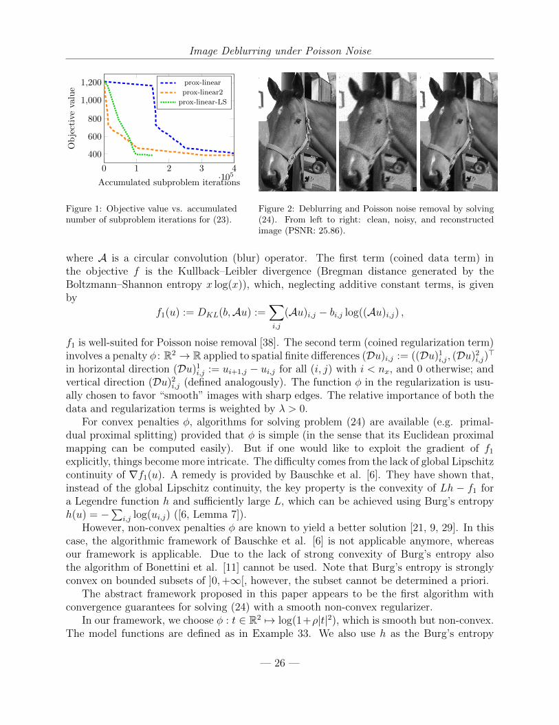
Image Deblurring under Poisson Noise
0 1 2 3 4·105
400
600
800
1,000
1,200
Accumulated subproblem iterations
Ob
ject
ive
valu
eprox-linear
prox-linear2
prox-linear-LS
Figure 1: Objective value vs. accumulatednumber of subproblem iterations for (23).
Figure 2: Deblurring and Poisson noise removal by solving(24). From left to right: clean, noisy, and reconstructedimage (PSNR: 25.86).
where A is a circular convolution (blur) operator. The first term (coined data term) inthe objective f is the Kullback–Leibler divergence (Bregman distance generated by theBoltzmann–Shannon entropy x log(x)), which, neglecting additive constant terms, is givenby
f1(u) := DKL(b,Au) :=∑i,j
(Au)i,j − bi,j log((Au)i,j) ,
f1 is well-suited for Poisson noise removal [38]. The second term (coined regularization term)involves a penalty φ : R2 → R applied to spatial finite differences (Du)i,j := ((Du)1
i,j, (Du)2i,j)>
in horizontal direction (Du)1i,j := ui+1,j − ui,j for all (i, j) with i < nx, and 0 otherwise; and
vertical direction (Du)2i,j (defined analogously). The function φ in the regularization is usu-
ally chosen to favor “smooth” images with sharp edges. The relative importance of both thedata and regularization terms is weighted by λ > 0.
For convex penalties φ, algorithms for solving problem (24) are available (e.g. primal-dual proximal splitting) provided that φ is simple (in the sense that its Euclidean proximalmapping can be computed easily). But if one would like to exploit the gradient of f1
explicitly, things become more intricate. The difficulty comes from the lack of global Lipschitzcontinuity of ∇f1(u). A remedy is provided by Bauschke et al. [6]. They have shown that,instead of the global Lipschitz continuity, the key property is the convexity of Lh − f1 fora Legendre function h and sufficiently large L, which can be achieved using Burg’s entropyh(u) = −
∑i,j log(ui,j) ([6, Lemma 7]).
However, non-convex penalties φ are known to yield a better solution [21, 9, 29]. In thiscase, the algorithmic framework of Bauschke et al. [6] is not applicable anymore, whereasour framework is applicable. Due to the lack of strong convexity of Burg’s entropy alsothe algorithm of Bonettini et al. [11] cannot be used. Note that Burg’s entropy is stronglyconvex on bounded subsets of ]0,+∞[, however, the subset cannot be determined a priori.
The abstract framework proposed in this paper appears to be the first algorithm withconvergence guarantees for solving (24) with a smooth non-convex regularizer.
In our framework, we choose φ : t ∈ R2 7→ log(1+ρ|t|2), which is smooth but non-convex.The model functions are defined as in Example 33. We also use h as the Burg’s entropy
— 26 —

Structured Matrix Factorization
to generate the Bergman proximity function (see Example 41). Thus, the subproblems (5)which emerge from linearizing the objective f in (24) around the current iterate u
u = argminu∈Rnx×ny
〈u− u,∇f(u)〉+1
τ
∑i,j
(ui,jui,j− log
(ui,jui,j
))can be solved exactly in closed-form ui,j = ui,j/(1 + τ(∇f(u))i,jui,j) for all i, j. A result forthe successful Poisson noise removal and deblurring is shown in Figure 2.
6.3 Structured Matrix Factorization
Structured matrix factorization problems are crucial in data analysis. It has many applica-tions in various areas including blind deconvolution in signal processing, clustering, sourceseparation, dictionary learning, etc.. There is a large body of literature on the subject andwe refer to e.g. [17, 15, 37, 39] and references therein for a comprehensive account.
The problem. Given a data matrix A ∈ RM×N whose N M -dimensional columns are thedata vectors. The goal is to find two matrices U ∈ RM×K and Z ∈ RK×N such that
A = UZ +Q ,
where Q ∈ RM×N accounts for an unknown error. The matrices U and Z (called also factors)enjoy features arising in a specific application at hand (see more below).
To solve the matrix factorization problem, we adopt the optimization approach and weconsider the non-convex and non-smooth minimization problem
minU∈U ,Z∈Z
f(A,UZ) + λg(Z) , f(A,UZ) :=1
2‖A− UZ‖2
F . (25)
The term f(A,UZ) stands for proximity function that measures fidelity of the approximationof A by the product UZ of the two factors. We here focus on the classical case where thefidelity is measured via the Frobenius norm ‖ · ‖F , but other data fidelity measures can alsobe used just as well in our framework, such as divergences (see [17] and references therein).The sets U , Z, which are non-empty closed and convex, and the function g ∈ Γ0 are used tocapture specific features of the matrices U and Z arising in a specific application as we willexemplify shortly. The influence of g is weighted by the parameter λ > 0.
Many (if not most) algorithms to solve the matrix factorization problem (25) are basedon Gauss-Seidel alternating minimization with limited convergence guarantees [17, 15, 37]4.The PALM algorithm proposed recently by Bolte et al. [10], was designed specifically forthe structure of the optimization problem (25). It can then be successfully applied to solve
4For very specific instances, a recent line of research proposes to lift the problem to the space of low-rankmatrices, and then use convex relaxation and computationally intensive conic programming that are onlyapplicable to small-dimensional problems; see, e.g., [1] for blind deconvolution.
— 27 —

Structured Matrix Factorization
instances of such a problem with provably guaranteed convergence under some assumptionsincluding the Kurdyka- Lojasiewicz property. However, though it can handle non-convexconstraint sets and functions g, it does not allow to incorporate Bregman proximity functions.
In the following, we show how our algorithmic framework can be applied to a broad classof matrix factorization instances. In particular, a distinctive feature of our algorithm is thatit can naturally and readily accommodate for different Bregman proximity functions and ithas no restrictions on the choice of the step size parameters (except positivity). A descentis enforced in the line search step, which follows the proximal step.
A generic algorithm. We apply Algorithm 1 to solve this problem, where the model func-tions are chosen to linearize the data fidelity function f(A,UZ), according to Example 33.The convex subproblems to be solved in the algorithm have the following form:
(U , Z) = argminU∈U ,Z∈Z
λg(Z)+⟨Z − Z, U>(U Z − A)
⟩F
+DhZ (Z, Z)
+⟨U − U , (U Z − A)Z>
⟩F
+DhU (U, U)
where 〈·, ·〉F stands for the Frobenius inner product. The Bregman proximity functionsDhZ (·, ·) and DhU (·, ·) provide the flexibility to handle a variety of constraint sets U andZ. In the following, we list different choices for the constraint sets and explain how toincorporate them into the optimization procedure. Due to the structure of the optimizationproblem, the variables U and Z can be handled separately. The only coupling is the datafidelity function f , which is linearized and therefore easy to incorporate.
Examples of constraints U . There are many possible choices for the set U depending onthe application at hand.
• Unconstrained case:U1 = RM×K .
In the unconstrained case, a suitable Bregman proximity function is given by theEuclidean distance DhU (U, U) = 1
2τU‖U − U‖2
F with step size parameter τU . Theresulting update step with respect to the dictionary U is a gradient descent step.
• Zero-mean and normalization:
U2 =
U ∈ RM×K | ∀j :
M∑i=1
U2i,j ≤ 1 ,∀j ≥ 2:
M∑i=1
Ui,j = 0
.
This choice of the constraint set leads to a natural normalization of the columns ofU that removes the scale ambiguity due to bilinearity. This choice is very classical indictionary learning, see, e.g., [39]. As in dictionary learning, the average of the firstcolumn may not be enforced to be zero, in order to allow the first column to absorbthe mean value of the data points.
— 28 —

Structured Matrix Factorization
By separability of U2, the Euclidean projection onto it is simple. This projector iscolumn-wise achieved by subtracting the mean, and then projecting the result ontothe Euclidean unit ball. Thus we advocate DhU (U, U) = 1
2τU‖U − U‖2
F with step sizeparameter τU . In turn, the subproblem with respect to U amounts to a projectedgradient descent step.
• Non-negativity and normalization:
U3 =
U ∈ RM×K | ∀j :
M∑i=1
Ui,j = 1 , ∀i, j : Ui,j ≥ 0
.
This choice is adopted in non-negative matrix factorization (NMF) [24]. The constraintset U3 is column-wise a unit simplex constraint. This constraint can be convenientlyhandled by choosing DhU (U, U) = 1
τU
∑i,j Ui,j(log(Ui,j)− log(Ui,j))− Ui,j + Ui,j, which
is the Bregman function generated by the entropy hU(U) = 1τU
∑i,j Ui,j log(Ui,j) with
step size parameter τU . This is a more natural choice than the Euclidean proximitydistance. Indeed, the update step with respect to U results in
Ui,j =Ui,j exp(−τU(CU)i,j)∑Mp=1 Up,j exp(−τU(CU)p,j)
∀i = 1, . . . ,M ; ∀j = 1, . . . , K ,
where we use the shorthand notation CU := ∇Uf(A, UZ) = U>(U Z−A) for the partialgradient of f with respect to U . The exponential function is applied entry-wise, hencenaturally preserving positivity. Note that the Euclidean projector onto U3 necessitatesto compute the projector on the simplex which can be achieved with sorting [28].
Examples of constraints Z. There are also several possible choices for the set Z andregularizing function g depending on the application at hand.
• Unconstrained case:Z1 = RK×N and g(Z) = 0 .
This case can be handled using a gradient descent step, analogously to the relatedupdate step with the constraint set U1.
• Non-negativity:
Z2 =Z ∈ RK×N | ∀i, j : Zi,j ≥ 0
and g(Z) = 0 .
This constraint is used in conjunction with U3 in NMF. It can be handled either witha Euclidean proximity function (which amounts to projecting on the non-negative or-thant), or via a Bregman proximity function DhZ (Z, Z) generated by the Boltzmann–Shannon entropy (hZ(Z) = 1
τZ
∑i,j Zi,j log(Zi,j)) or, alternatively, Burg’s entropy
— 29 —

Structured Matrix Factorization
(hZ(Z) = − 1τZ
∑i,j log(Zi,j)), with step size parameter τZ . The update with respect
to Z then reads
Zi,j = Zi,j exp(−τZ(CZ)i,j) ∀i = 1, . . . , K ; ∀j = 1, . . . , N ,
where we use the shorthand notation CZ := ∇Zf(A, UZ) = (U Z−A)Z> for the partialgradient of f with respect to Z.
• Sparsity constraints:
Z3 = RK×N and g(Z) = ‖Z‖1 .
The introduction of sparsity has been of prominent importance in several matrix fac-torization problems, including dictionary learning [34], NMF [23] 5 and source sepa-ration [37]. The Euclidean proximal mapping of the `1-norm is the entry-wise soft-thresholding, hence giving the update step with respect to Z as
Zi,j = max0, 1−λτZ/|Zi,j−τZ(CZ)i,j|(Zi,j−τZ(CZ)i,j) ∀i = 1, . . . , K ; ∀j = 1, . . . , N .
• Low rank constraint:
Z3 = RK×N and g(Z) = ‖Z‖∗ .
The nuclear norm or 1-Schatten norm ‖Z‖∗ is the sum of the singular values. It isknown to be the tightest convex relaxation to the rank and was shown to promotelow rank solutions [35]. Such a regularization would be useful in the situation wherecolumns of A are (to a good approximation) clustered on a few linear subspaces spannedby the columns of U , i.e. the columns of A can be explained by columns of U from thesame subspace (“cluster”).
The Euclidian proximal mapping of the nuclear norm is the soft-thresholding appliedto the singular values. In turn, the update step with respect to Z reads
Zi,j = Wdiag((max0, 1− λτZ/σiσi)i)V >,
where W , V are respectively the matrices of left and right singular vectors of Z−τZCZ ,and σ is the associated vector of singular values.
5Strictly speaking, Z3 should be the non-negative orthant for sparse NMF. But this does not changeanything to our discussion since computing the Euclidean proximal mapping of the `1 norm restricted to thenon-negative orthant is easy.
— 30 —

Conclusions
7 Conclusions
We have presented an algorithmic framework, that unifies the analysis of several first orderoptimization algorithms in non-smooth non-convex optimization such as Gradient Descent,Forward–Backward Splitting, ProxDescent, and many more. The algorithm combines se-quential Bregman proximal minimization of model functions, which is the key concept forthe unification, with an Armijo-like line search strategy. The framework reduces the differ-ence between algorithms to the model approximation error measured by a growth function.For the developed abstract algorithmic framework, we establish subsequential convergenceto a stationary point and demonstrate its flexible applicability in several difficult inverseproblems from machine learning, signal and image processing.
References
[1] A. Ahmed, B. Recht, and J. Romberg. Blind deconvolution using convex programming. IEEETransactions on Information Theory, 60(3):1711–1732, 2014.
[2] H. Attouch, J. Bolte, and B. Svaiter. Convergence of descent methods for semi-algebraicand tame problems: proximal algorithms, forward–backward splitting, and regularized Gauss–Seidel methods. Mathematical Programming, 137(1-2):91–129, 2013.
[3] H. Bauschke and J. Borwein. Legendre functions and the method of random Bregman projec-tions. Journal of Convex Analysis, 4(1):27–67, 1997.
[4] H. Bauschke, J. Borwein, and P. Combettes. Essential smoothness, essential strict convexity,and Legendre functions in Banach spaces. Communications in Contemporary Mathematics,3(4):615–647, Nov. 2001.
[5] H. Bauschke, J. Borwein, and P. Combettes. Bregman monotone optimization algorithms.SIAM Journal on Control and Optimization, 42(2):596–636, Jan. 2003.
[6] H. H. Bauschke, J. Bolte, and M. Teboulle. A descent lemma beyond Lipschitz gradient con-tinuity: First-order methods revisited and applications. Mathematics of Operations Research,42(2):330–348, Nov. 2016.
[7] H. H. Bauschke and P. L. Combettes. Convex analysis and monotone operator theory in Hilbertspaces. Springer, 2011.
[8] M. Bertero, P. Boccacci, G. Desidera, and G. Vicidomini. Image deblurring with Poisson data:from cells to galaxies. Inverse Problems, 25(12):123006, 2009.
[9] A. Blake and A. Zisserman. Visual Reconstruction. MIT Press, Cambridge, MA, 1987.
[10] J. Bolte, S. Sabach, and M. Teboulle. Proximal alternating linearized minimization for non-convex and nonsmooth problems. Mathematical Programming, 146(1-2):459–494, 2014.
[11] S. Bonettini, I. Loris, F. Porta, and M. Prato. Variable metric inexact line-search basedmethods for nonsmooth optimization. SIAM Journal on Optimization, 26(2):891–921, Jan.2016.
[12] L. M. Bregman. The relaxation method of finding the common point of convex sets andits application to the solution of problems in convex programming. USSR ComputationalMathematics and Mathematical Physics, 7(3):200–217, 1967.
— 31 —

References
[13] J. Burg. The relationship between maximum entropy spectra and maximum likelihood spectra.Geophysics, 37(2):375–376, Apr. 1972.
[14] A. Chambolle. An algorithm for total variation minimization and applications. Journal ofMathematical Imaging and Vision, 20:89–97, 2004.
[15] S. Chaudhuri, R. Velmurugan, and R. Rameshan. Blind Image Deconvolution. Springer, 2014.
[16] G. Chen and M. Teboulle. Convergence analysis of proximal-like minimization algorithm usingbregman functions. SIAM Journal on Optimization, 3:538–543, 1993.
[17] A. Cichocki, R. Zdunek, A. Phan, and S. Amari. Nonnegative Matrix and Tensor Factor-izations: Applications to Exploratory Multi-Way Data Analysis and Blind Source Separation.Wiley,, New York, 2009.
[18] P. Combettes, D. Dung, and B. Vu. Dualization of signal recovery problems. Set-Valued andVariational Analysis, 18(3-4):373–404, Dec. 2010.
[19] D. Drusvyatskiy, A. D. Ioffe, and A. S. Lewis. Nonsmooth optimization using Taylor-likemodels: error bounds, convergence, and termination criteria. ArXiv e-prints, Oct. 2016. arXiv:1610.03446.
[20] D. Drusvyatskiy and A. S. Lewis. Error bounds, quadratic growth, and linear convergence ofproximal methods. ArXiv e-prints, Feb. 2016. arXiv:1602.06661.
[21] S. Geman and D. Geman. Stochastic relaxation, Gibbs distributions, and the Bayesian restora-tion of images. IEEE Transactions on Pattern Analysis and Machine Intelligence, 6:721–741,1984.
[22] F. R. Hampel, E. M. Ronchetti, P. J. Rousseeuw, and W. A. Stahel. Robust Statistics: TheApproach Based on Influence Functions. MIT Press, Cambridge, MA, 1986.
[23] P. Hoyer. Non-negative matrix factorization with sparseness constraints. J. Mach. Learn. Res.,5:1457–1469, 2004.
[24] D. Lee and H. Seung. Learning the part of objects from nonnegative matrix factorization.Nature, 401:788–791, 1999.
[25] A. Lewis and S. Wright. A proximal method for composite minimization. MathematicalProgramming, 158(1-2):501–546, July 2016.
[26] P. L. Lions and B. Mercier. Splitting algorithms for the sum of two nonlinear operators. SIAMJournal on Applied Mathematics, 16(6):964–979, 1979.
[27] D. Marquardt. An algorithm for least-squares estimation of nonlinear parameters. Society forIndustrial and Applied Mathematics, 11:431–441, 1963.
[28] C. Michelot. A finite algorithm for finding the projection of a point onto the canonical simplexof Rn. J. Optim. Theory Appl., 50:195–200, 1986.
[29] D. Mumford and J. Shah. Optimal approximations by piecewise smooth functions and asso-ciated variational problems. Communications on Pure and Applied Mathematics, 42:577–685,1989.
[30] Q. Nguyen. Forward–Backward Splitting with Bregman Distances. Vietnam Journal of Math-ematics, pages 1–21, Jan. 2017.
[31] D. Noll. Convergence of non-smooth descent methods using the Kurdyka– Lojasiewicz inequal-ity. Journal of Optimization Theory and Applications, 160(2):553–572, Sept. 2013.
— 32 —
References
[32] D. Noll, O. Prot, and P. Apkarian. A proximity control algorithm to minimize nonsmooth andnonconvex functions. Pacific Journal of Optimization, 4(3):571–604, 2008.
[33] P. Ochs, A. Dosovitskiy, T. Brox, and T. Pock. On iteratively reweighted algorithms fornonsmooth nonconvex optimization in computer vision. SIAM Journal on Imaging Sciences,8(1):331–372, 2015.
[34] B. Olshausen and D. Field. Sparse coding with an overcomplete basis set: A strategy employedby V1? Vision Research., 37, 1996. 3311–3325.
[35] B. Recht, M. Fazel, and P. A. Parrilo. Guaranteed minimum-rank solutions of linear matrixequations via nuclear norm minimization. SIAM review, 52(3):471–501, 2010.
[36] R. T. Rockafellar and R.-B. Wets. Variational Analysis, volume 317. Springer Berlin Heidel-berg, Heidelberg, 1998.
[37] J.-L. Starck, F. Murtagh, and J. Fadili. Sparse image and signal processing: wavelets, curvelets,morphological diversity. Cambridge University Press, 2nd edition, 2015.
[38] Y. Vardi, L. Shepp, and L. Kaufman. A statistical model for positron emission tomography.Journal of the American Statistical Association, 80(389):8–20, 1985.
[39] Y. Xu, Z. Li, J. Yang, and D. Zhang. A survey of dictionary learning algorithms for facerecognition. IEEE Access, 5:8502–8514, 2017.
[40] R. Zanella, P. Boccacci, L. Zanni, and M. Bertero. Efficient gradient projection methods foredge-preserving removal of Poisson noise. Inverse Problems, 25(4), 2009.
— 33 —