Embed Size (px)
Citation preview
Physica D 184 (2003) 64–85
Non-stationary spectra of local wave turbulence
Colm Connaughtona,∗, Alan C. Newella,b, Yves Pomeaub,ca Mathematics Institute, University of Warwick, Coventry CV4 7AL, UK
b Department of Mathematics, University of Arizona, Tucson, AZ 85721, USAc Lab. Physique Statistique, E.N.S., 24 Rue Lhomond, 75231 Paris Cedex 05, France
Abstract
The evolution of the Kolmogorov–Zakharov (K–Z) spectrum of weak turbulence is studied in the limit of strongly localinteractions where the usual kinetic equation, describing the time evolution of the spectral wave-action density, can beapproximated by a PDE. If the wave action is initially compactly supported in frequency space, it is then redistributed byresonant interactions producing the usual direct and inverse cascades, leading to the formation of the K–Z spectra. Theemphasis here is on the direct cascade. The evolution proceeds by the formation of a self-similar front which propagates to theright leaving a quasi-stationary state in its wake. This front is sharp in the sense that the solution remains compactly supporteduntil it reaches infinity. If the energy spectrum has infinite capacity, the front takes infinite time to reach infinite frequency andleaves the K–Z spectrum in its wake. On the other hand, if the energy spectrum has finite capacity, the front reaches infinitywithin a finite time,t∗, and the wake is steeper than the K–Z spectrum. For this case, the K–Z spectrum is set up from theright after the front reaches infinity. The slope of the solution in the wake can be related to the speed of propagation of thefront. It is shown that the anomalous slope in the finite capacity case corresponds to the unique front speed which ensuresthat the front tip contains a finite amount of energy as the connection to infinity is made. We also introduce, for the first time,the notion of entropy production in wave turbulence and show how it evolves as the system approaches the stationary K–Zspectrum.© 2003 Elsevier B.V. All rights reserved.
Keywords:Kolmogorov–Zakharov spectrum; Non-stationary; Wave turbulence
1. Introduction and motivation
Wave turbulence is concerned with the statistical description of an infinite sea of dispersive waves, which areweakly coupled by nonlinear interactions and maintained away from equilibrium by interaction with sources andsinks of energy. The theory has found practical application in many branches of physics including the descriptionof surface waves on fluid interfaces[3,7,8,13], Alfven wave turbulence in astrophysical plasmas[6,12], nonlinearoptics[4] and acoustics[10,14] to name a few.
The central quantity of theoretical interest is the spectral wave-action density,nk, which describes how theexcitations in the system are distributed among different wave-vectors,k. Under fairly weak assumptions[11], the
∗ Corresponding author.E-mail address:[email protected] (C. Connaughton).
0167-2789/$ – see front matter © 2003 Elsevier B.V. All rights reserved.doi:10.1016/S0167-2789(03)00213-6
C. Connaughton et al. / Physica D 184 (2003) 64–85 65
long time behaviour ofnk is given by an equation known as the wave kinetic equation. For a system dominated byfour wave interactions this equation takes the form
∂nk
∂t= 4π
∫|Tkk1k2k3|2F4[nk] (k + k1 − k2 − k3)dk1 dk2 dk3, (1)
where
F4[nk] = nknk1nk2nk3
(1
nk+ 1
nk1
− 1
nk2
− 1
nk3
)(ωk + ωk1 − ωk2 − ωk3). (2)
Eq. (1)is the analogue for waves of the Boltzmann equation of classical statistical mechanics. In many applications,ωk andTkk1k2k3 are homogeneous functions of their arguments. Their degrees of homogeneity shall be denoted byα andγ, respectively. Under rescaling,k → λk, they transform as follows:
ωλk = λαωk, (3)
Tλkλk1λk2λk3 = λγTkk1k2k3. (4)
It was shown by Zakharov et al.[15] in the 1960s that if the energy sources and sinks are separated by an “inertialrange”,Eq. (1)has exact isotropic steady-state solutions
nk = c1P1/3k−(2γ+3d)/3, (5)
nk = c2Q1/3k−(2γ+3d−1)/3, (6)
which carry constant fluxes of conserved densities, in this case energy flux,P , or wave-action flux,Q, betweensources and sinks. These steady-state spectra are the direct analogues of the direct and inverse cascades in hydro-dynamic turbulence and are referred to as Kolmogorov–Zakharov (K–Z) spectra. They have been well observedexperimentally in a variety of contexts.
In 1991, Falkovich and Shafarenko[5] addressed the question of how the K–Z spectrum is set up in time ifnk
is initially compactly supported in wave-vector space. They used a self-similar solution of(1) and an assumptionthat, for the direct cascade, the total energy increases linearly in time, to show that(5) is set up by a nonlinear frontwhich propagates towardsk = ∞ and leaves thek−(2γ+3d)/3 spectrum in its wake.
However, subsequent numerical simulations of the kinetic equation for Alfven wave turbulence performed byGaltier et al.[6] suggested that the development of the K–Z spectrum may proceed by a different route. For theAlfven wave system, the K–Z energy spectrum has finite energy capacity, meaning that on the K–Z spectrum,∫E(k)dk < ∞. This implies that the nonlinear front must reachk = ∞ within a finite time,t∗. They noticed
that the spectrum in the wake of the front was significantly steeper than the K–Z value for times less than thesingular time,t∗, and that the K–Z spectrum then developed from right to left after the front reachedk = ∞. Otherwork by Pomeau and co-workers[9] on the inverse cascade in the nonlinear Schrodinger equation suggested thatthere might be anomalous quasi-stationary spectra associated with non-stationary solutions of kinetic equations.However, no-one has yet made a specific attempt to search for them.
One of the challenges in far-from-equilibrium systems is to understand the means by which stationary states arereached and to ask if there are functional analogous to the entropy in equilibrium systems. What we will show isthat while the entropy, which for wave turbulence is formally (see for example,[2])
S =∫
ln nk dk (7)
is not well-defined on the steady-state solutions, spectra(5) and (6), its production rate is. We find that for 0< t < t∗,when the spectrum in the wake of the front is steeper than the K–Z spectrum, the entropy production is positive. At
66 C. Connaughton et al. / Physica D 184 (2003) 64–85
t∗ the connection tok = ∞ is made and energy is no longer a conserved quantity. Fort > t∗, the K–Z spectrumis established via a front which travels back fromk = ∞. During this stage, the entropy production rate, whilestill positive, gradually decreases and asymptotes to zero, its value on the exact K–Z spectrum. We conjecture thatthis scenario, established in this paper for the differential approximation to the kinetic equation,(1), will be widelyvalid for finite capacity non-equilibrium systems, including three-dimensional hydrodynamic turbulence at largeReynolds numbers.
This leads us to the topic of this article. We have made an extensive study of the non-stationary solutions of theso-called differential kinetic equation of local wave turbulence.1 This model equation is obtained from(1) under theassumption that the interaction co-efficient,Tkk1k2k3 is strongly localised inkk1k2k3 space. It has the advantage ofreplacing the integro-differential kinetic equation with a PDE. We find that the qualitative behaviour observed byGaltier et al. is present in this model in the finite capacity case. Since we are dealing with a PDE, we can go a lotfurther in terms of understanding.
The organisation of the article is as follows. InSection 2we introduce the differential kinetic equation and describea few of its properties which make it a good model of wave turbulence. We also introduce exact expressions for thefluxes of energy (P), the flux of particles (Q), and the entropy production rate in terms of its flux (R) and its bulkproduction rate (T ). The latter is always positive definite. We calculate each of these quantities on the algebraicsolutions,nk ∝ k−αx. Section 3contains the details of some numerical simulations of the PDE. These simulationssuggest that the nonlinear front is “sharp” in the sense thatnk remains compactly supported fort < t∗. There is asingularity, a divergence in the second derivative in fact, at the front tip between the regionsnk = 0 andnk > 0.Next, in Section 4, we construct a family of self-similar solutions of the differential kinetic equation which areparameterised by a single free parameter. This free parameter can be interpreted as the asymptotic slope behind thefront. Following that, inSection 5, we use this self-similarity analysis to formulate a hypothesis which we call thecritical front speed hypothesis. This hypothesis is based on physical arguments and allows us to select a criticalvalue,xc, for the asymptotic slope, given by
xc = x0 + 2γ − 3α
12α, (8)
wherex0 denotes the usual K–Z exponent for the direct cascade. This formula is well supported by our numer-ical simulations. In our conclusion, we attempt to make a connection with entropy production arguments. Twoappendices are provided. InAppendix A, we analyse the mathematical structure of the similarity equation and tryto understand how the critical slope is related to the solution trajectories of the underlying ordinary differentialequation.Appendix Bgives a brief outline of the numerical methods used.
2. The differential kinetic equation
We begin by briefly discussing the origin of the differential kinetic equation. Assuming that the wave-actionspectrum rapidly becomes isotropic, and averaging over angles, we can make a transformation fromd-dimensionalwave-vector space to frequency space
∂Nω
∂t=∫Sωω1ω2ω3F4[nω] dω1 dω2 dω3, (9)
1 We have subsequently analysed a second-order model equation whose structure is similar to that of the differential kinetic equation studied inthis paper but is analytically and numerically more tractable. We have found qualitatively similar behaviour. However, the value of the anomalousexponent appears to differ from that which would be predicted by our critical front speed hypothesis.
C. Connaughton et al. / Physica D 184 (2003) 64–85 67
where
Sωω1ω2ω3 = 4π∫
|Tkk1k2k3|2 (k + k1 − k2 − k3)(kk1k2k3)d−1 dk
dω
dk1
dω1
dk2
dω2
dk3
dω3dΩ (10)
andNω is defined by requiring that∫φ(ω)Nω dω =
∫φ(|k|α)nk dk (11)
for any test function,φ. Here the volume element dΩ represents integration over the angular variables inkk1k2k3
space and the wave-vector moduli are related to the frequency via the dispersion relation
ωk = ckα. (12)
If we assume that the interaction coefficient,Tkk1k2k3 is strongly local inkk1k2k3 space then(9)can be approximatedby a differential equation[4]
∂Nω
∂t= I
∂2
∂ω2
(ωsn4
ω
∂2
∂ω2
(1
nω
)), (13)
where
nω(t) = n(k(ω), t), (14)
s = 3x0 + 2, (15)
x0 = 2γ + 3d
3α. (16)
I is a pure number which comes from the angular integrations in(10). This equation is called the differential kineticequation.
The local approximation leading to the differential kinetic equation,(13), is rather drastic and is not justified formany of the physical applications of weak turbulence. Nonetheless, it retains many of the qualitative features of thefull kinetic equation (9). It provides an excellent model in the context of which these features can be easily studied.In particular, the differential kinetic equation respects the conservation laws embodied within its integro-differentialprecursor, namely the conservation of the total energy
E =∫ωNω dω (17)
and the total number of particles is
N =∫Nω dω. (18)
It also preserves the scaling and homogeneity properties of the kinetic equation. Consequently, the pure scalingsolutions of the kinetic equation, the equilibrium thermodynamic spectra and the non-equilibrium K–Z spectra, arealso solutions of the differential kinetic equation. These solutions are of the formnω = cω−x wherex takes one ofthe following values:
x = 1, x = 0 (thermodynamic)
or
x = 2γ + 3d
3α, x = 2γ + 3d − α
3α(K–Z).
68 C. Connaughton et al. / Physica D 184 (2003) 64–85
It is convenient to define
K[nω] = ω3x0+2n4ω
∂2
∂ω2
(1
nω
). (19)
The two conservation laws can be written as continuity equations:
∂Nω
∂t− ∂Q
∂ω= 0, (20)
∂Eω
∂t+ ∂P
∂ω= 0, (21)
where
Q = ∂K
∂ω(22)
is the local flux of particles,
P = K− ω∂K
∂ω(23)
is the local flux of energy and
Eω = ωNω (24)
is the energy density if frequency space. Note thatP is defined to be positive when energy flows to the right inω
space andQ is positive when particles flow to the left.The entropy,S, of a wave system is formally
∫ln nk dk. The production rate is
∂S
∂t= d
dt
∫ln nk dk =
∫1
nω
dNω∂t
dω (25)
and can readily be calculated to be
S = −∂R∂ω
+ T. (26)
The entropy flux,R, which is positive for entropy flow to large wavenumbers, is
R = −Q
n2ω
∂
∂ω(ωnω)− P
n2ω
∂nω
∂ω(27)
and the local bulk entropy production rate,T , is
T = Iω3x0+2n4ω
(∂2
∂ω2
(1
nω
))2
. (28)
Note thatT is positive definite and zero on the thermodynamic solution,nω = τ/(ω− µ), τ being the temperatureandµ the chemical potential. Indeed if the system were isolated, say on the intervalω1 < ω < ω2, andP ,Q andR were identically zero, then the usual principles of equilibrium systems would apply.
On the solutionnω = cω−x, the quantitiesK,Q, P , R, T and−(∂R/∂ω)+ T are calculated. They are
K = Ic3ω3x0−3xx(x− 1), (29)
Q = 3Ic3x(x− 1)(x0 − x)ω3x0−3x−1, (30)
C. Connaughton et al. / Physica D 184 (2003) 64–85 69
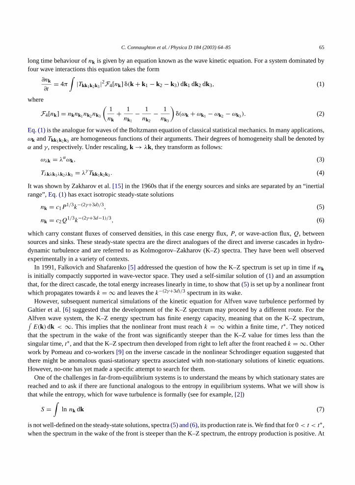
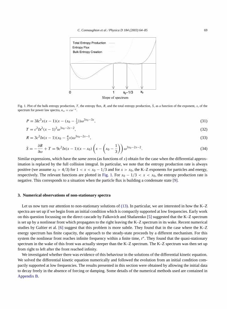
Fig. 1. Plot of the bulk entropy production,T , the entropy flux,R, and the total entropy production,S, as a function of the exponent,x, of thespectrum for power law spectra,nω = cω−x.
P = 3Ic3x(x− 1)(x− (x0 − 13))ω
3x0−3x, (31)
T = c2Ix2(x− 1)2ω3x0−2x−2, (32)
R = 3c2Ix(x− 1)(x0 − 43x)ω
3x0−2x−1, (33)
S = −∂R∂ω
+ T = 9c2Ix(x− 1)(x− x0)
(x−
(x0 − 1
3
))ω3x0−2x−2. (34)
Similar expressions, which have thesamezeros (as functions ofx) obtain for the case when the differential approx-imation is replaced by the full collision integral. In particular, we note that the entropy production rate is alwayspositive (we assumex0 > 4/3) for 1< x < x0 − 1/3 and forx > x0, the K–Z exponents for particles and energy,respectively. The relevant functions are plotted inFig. 1. For x0 − 1/3 < x < x0, the entropy production rate isnegative. This corresponds to a situation when the particle flux is building a condensate state[9].
3. Numerical observations of non-stationary spectra
Let us now turn our attention to non-stationary solutions of(13). In particular, we are interested in how the K–Zspectra are set up if we begin from an initial condition which is compactly supported at low frequencies. Early workon this question focussing on the direct cascade by Falkovich and Shafarenko[5] suggested that the K–Z spectrumis set up by a nonlinear front which propagates to the right leaving the K–Z spectrum in its wake. Recent numericalstudies by Galtier et al.[6] suggest that this problem is more subtle. They found that in the case where the K–Zenergy spectrum has finite capacity, the approach to the steady-state proceeds by a different mechanism. For thissystem the nonlinear front reaches infinite frequency within a finite time,t∗. They found that the quasi-stationaryspectrum in the wake of this front was actually steeper than the K–Z spectrum. The K–Z spectrum was then set upfrom right to left after the front reached infinity.
We investigated whether there was evidence of this behaviour in the solutions of the differential kinetic equation.We solved the differential kinetic equation numerically and followed the evolution from an initial condition com-pactly supported at low frequencies. The results presented in this section were obtained by allowing the initial datato decay freely in the absence of forcing or damping. Some details of the numerical methods used are contained inAppendix B.
70 C. Connaughton et al. / Physica D 184 (2003) 64–85
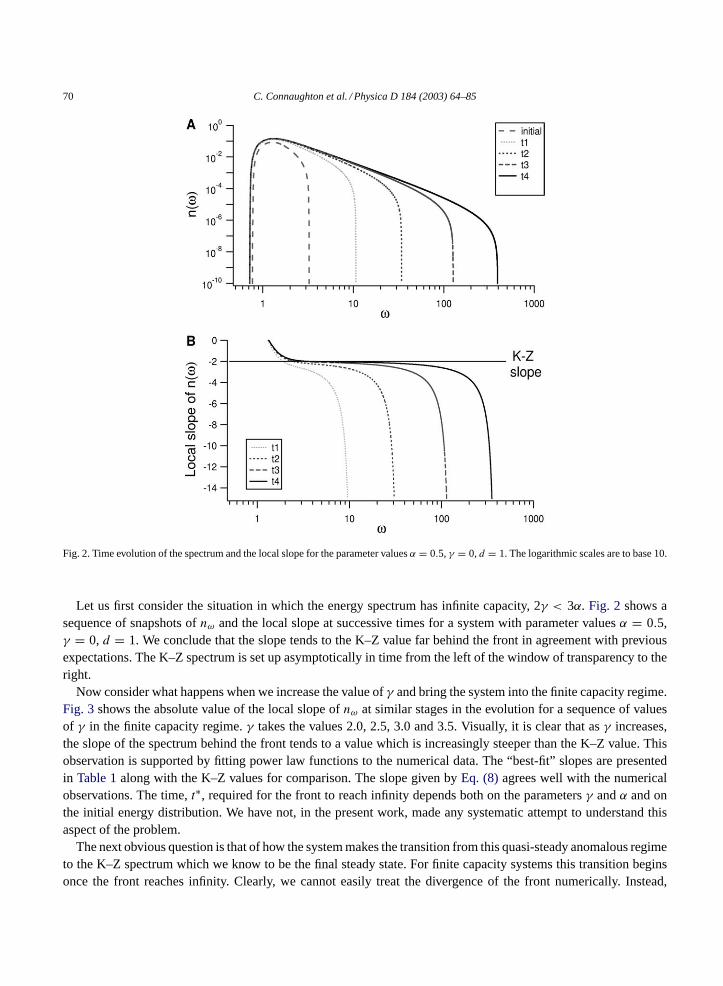
Fig. 2. Time evolution of the spectrum and the local slope for the parameter valuesα = 0.5,γ = 0,d = 1. The logarithmic scales are to base 10.
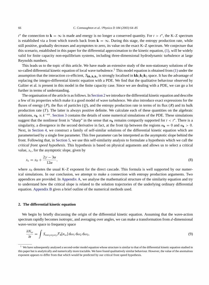
Let us first consider the situation in which the energy spectrum has infinite capacity, 2γ < 3α. Fig. 2 shows asequence of snapshots ofnω and the local slope at successive times for a system with parameter valuesα = 0.5,γ = 0, d = 1. We conclude that the slope tends to the K–Z value far behind the front in agreement with previousexpectations. The K–Z spectrum is set up asymptotically in time from the left of the window of transparency to theright.
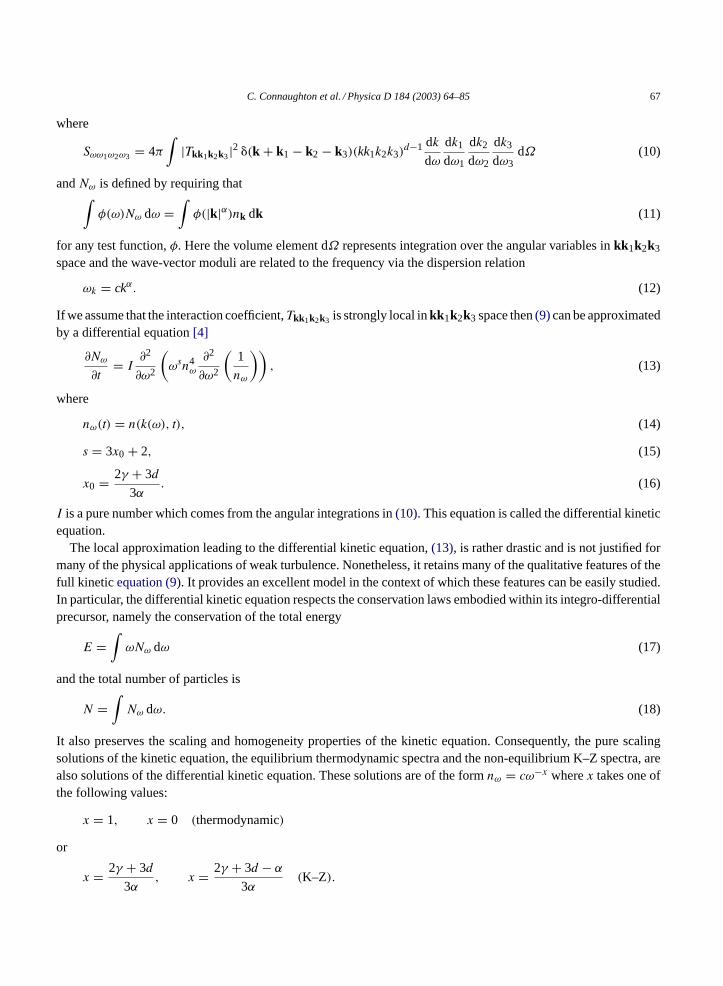
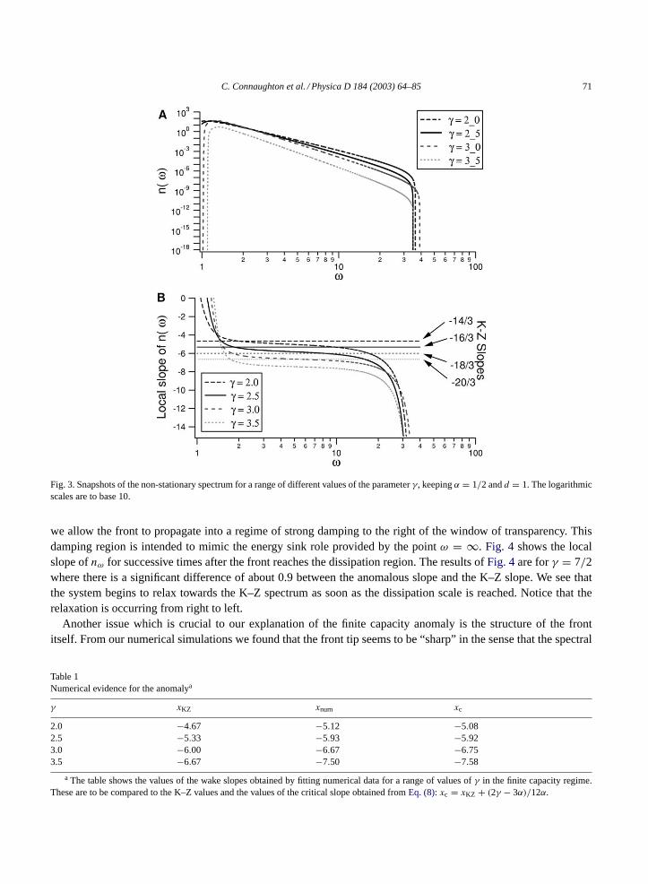
Now consider what happens when we increase the value ofγ and bring the system into the finite capacity regime.Fig. 3shows the absolute value of the local slope ofnω at similar stages in the evolution for a sequence of valuesof γ in the finite capacity regime.γ takes the values 2.0, 2.5, 3.0 and 3.5. Visually, it is clear that asγ increases,the slope of the spectrum behind the front tends to a value which is increasingly steeper than the K–Z value. Thisobservation is supported by fitting power law functions to the numerical data. The “best-fit” slopes are presentedin Table 1along with the K–Z values for comparison. The slope given byEq. (8)agrees well with the numericalobservations. The time,t∗, required for the front to reach infinity depends both on the parametersγ andα and onthe initial energy distribution. We have not, in the present work, made any systematic attempt to understand thisaspect of the problem.
The next obvious question is that of how the system makes the transition from this quasi-steady anomalous regimeto the K–Z spectrum which we know to be the final steady state. For finite capacity systems this transition beginsonce the front reaches infinity. Clearly, we cannot easily treat the divergence of the front numerically. Instead,
C. Connaughton et al. / Physica D 184 (2003) 64–85 71
Fig. 3. Snapshots of the non-stationary spectrum for a range of different values of the parameterγ, keepingα = 1/2 andd = 1. The logarithmicscales are to base 10.
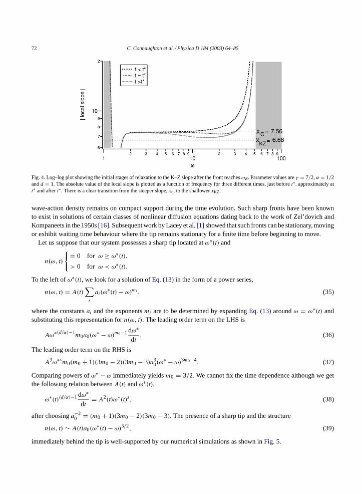
we allow the front to propagate into a regime of strong damping to the right of the window of transparency. Thisdamping region is intended to mimic the energy sink role provided by the pointω = ∞. Fig. 4 shows the localslope ofnω for successive times after the front reaches the dissipation region. The results ofFig. 4are forγ = 7/2where there is a significant difference of about 0.9 between the anomalous slope and the K–Z slope. We see thatthe system begins to relax towards the K–Z spectrum as soon as the dissipation scale is reached. Notice that therelaxation is occurring from right to left.
Another issue which is crucial to our explanation of the finite capacity anomaly is the structure of the frontitself. From our numerical simulations we found that the front tip seems to be “sharp” in the sense that the spectral
Table 1Numerical evidence for the anomalya
γ xKZ xnum xc
2.0 −4.67 −5.12 −5.082.5 −5.33 −5.93 −5.923.0 −6.00 −6.67 −6.753.5 −6.67 −7.50 −7.58
a The table shows the values of the wake slopes obtained by fitting numerical data for a range of values ofγ in the finite capacity regime.These are to be compared to the K–Z values and the values of the critical slope obtained fromEq. (8): xc = xKZ + (2γ − 3α)/12α.
72 C. Connaughton et al. / Physica D 184 (2003) 64–85
Fig. 4. Log–log plot showing the initial stages of relaxation to the K–Z slope after the front reachesωR. Parameter values areγ = 7/2,α = 1/2andd = 1. The absolute value of the local slope is plotted as a function of frequency for three different times, just beforet∗, approximately att∗ and aftert∗. There is a clear transition from the steeper slope,xc, to the shallowerxKZ .
wave-action density remains on compact support during the time evolution. Such sharp fronts have been knownto exist in solutions of certain classes of nonlinear diffusion equations dating back to the work of Zel’dovich andKompaneets in the 1950s[16]. Subsequent work by Lacey et al.[1] showed that such fronts can be stationary, movingor exhibit waiting time behaviour where the tip remains stationary for a finite time before beginning to move.
Let us suppose that our system possesses a sharp tip located atω∗(t) and
n(ω, t)
= 0 for ω ≥ ω∗(t),> 0 for ω < ω∗(t).
To the left ofω∗(t), we look for a solution ofEq. (13)in the form of a power series,
n(ω, t) = A(t)∑i
ai(ω∗(t)− ω)mi, (35)
where the constantsai and the exponentsmi are to be determined by expandingEq. (13)aroundω = ω∗(t) andsubstituting this representation forn(ω, t). The leading order term on the LHS is
Aω∗(d/α)−1m0a0(ω
∗ − ω)m0−1 dω∗
dt. (36)
The leading order term on the RHS is
A3ω∗sm0(m0 + 1)(3m0 − 2)(3m0 − 3)a30(ω
∗ − ω)3m0−4. (37)
Comparing powers ofω∗ − ω immediately yieldsm0 = 3/2. We cannot fix the time dependence although we getthe following relation betweenA(t) andω∗(t),
ω∗(t)(d/α)−1 dω∗
dt= A2(t)ω∗(t)s, (38)
after choosinga−20 = (m0 + 1)(3m0 − 2)(3m0 − 3). The presence of a sharp tip and the structure
n(ω, t) ∼ A(t)a0(ω∗(t)− ω)3/2, (39)
immediately behind the tip is well-supported by our numerical simulations as shown inFig. 5.
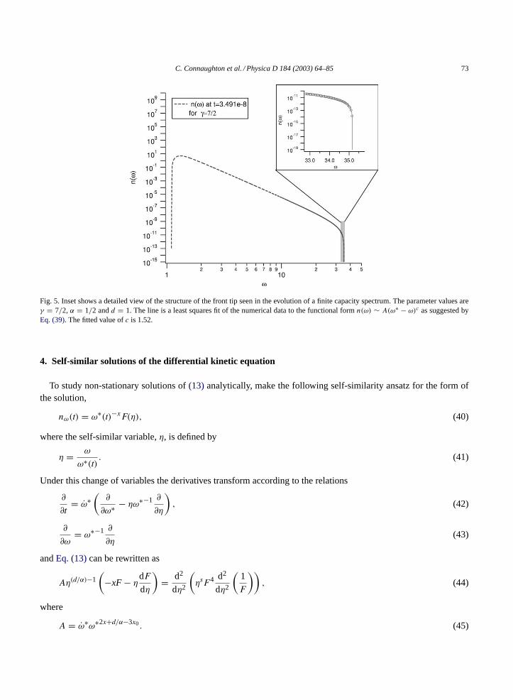
C. Connaughton et al. / Physica D 184 (2003) 64–85 73
Fig. 5. Inset shows a detailed view of the structure of the front tip seen in the evolution of a finite capacity spectrum. The parameter values areγ = 7/2, α = 1/2 andd = 1. The line is a least squares fit of the numerical data to the functional formn(ω) ∼ A(ω∗ − ω)c as suggested byEq. (39). The fitted value ofc is 1.52.
4. Self-similar solutions of the differential kinetic equation
To study non-stationary solutions of(13) analytically, make the following self-similarity ansatz for the form ofthe solution,
nω(t) = ω∗(t)−xF(η), (40)
where the self-similar variable,η, is defined by
η = ω
ω∗(t). (41)
Under this change of variables the derivatives transform according to the relations
∂
∂t= ω∗
(∂
∂ω∗ − ηω∗−1 ∂
∂η
), (42)
∂
∂ω= ω∗−1 ∂
∂η(43)
andEq. (13)can be rewritten as
Aη(d/α)−1(
−xF − ηdF
dη
)= d2
dη2
(ηsF4 d2
dη2
(1
F
)), (44)
where
A = ω∗ω∗2x+d/α−3x0. (45)
74 C. Connaughton et al. / Physica D 184 (2003) 64–85
Herex0 = (2γ + 3d)/3α is the exponent of the K–Z energy spectrum. The free parameter,x, is the asymptoticslope of the spectrum far behind the front. This is because we assume that there exists a quasi-stationary regime farbehind the front, which is a simple power law to leading order,nw ∼ ω−y. We must therefore havey = x in orderto cancel the time dependence from the leading order part of(40).
For a self-similar solution,A must be time independent. We are interested in situations where the system hasfinite energy capacity and generates a singularity within a finite time which we shall denote byt∗. The appropriatesolution of(45)describing such situations is
ω∗(t) = (t∗ − t)b. (46)
It is convenient to define
κd = 2γ − 3α
3α. (47)
The direct cascade has infinite energy capacity forκd < 0 and finite energy capacity forκd > 0. Upon substitutionof the form(46) into (45) it follows that
b = (2(x− x0)− κd)−1, (48)
A = −b. (49)
We can also define
κi = 2γ − α
3α, (50)
such that the inverse cascade has infinite particle capacity forκi > 0 and finite particle capacity forκi < 0.Eq. (48)can be written in the equivalent form
b = (2(x− x0 + 13)− κi)
−1 (51)
which is more appropriate for studying the inverse cascade. Notice that the speed of propagation of the front atω∗,as measured byb, is related to the asymptotic slope,x, behind the front.
If we are interested in the direct cascade thenω∗ → ∞ ast → t∗. This corresponds tob < 0. Conversely, forthe inverse cascade,ω∗ → 0 ast → t∗, corresponding tob > 0.
Upon substitution of(48) and (49)into (44)we obtain
(2(x− x0)− κd)−1η−1+d/α
(xF + η
dF
dη
)= d2
dη2
(ηsF4 d2
dη2
(1
F
)). (52)
Let us now consider the structure of the front tip in the self-similar variables. From our numerical simulations weexpect that there is a singularity in the solution asη → 1. For the direct cascade, we look for a singularity of theform (1 − η)m, approaching from the left. For the inverse cascade we expect a singularity of the form(η − 1)m
approaching from the right. Let us restrict our attention to the direct cascade.Consider an expansion of the solution to the left ofη = 1 in the form
F(η) = (1 − η)m∞∑n=0
an(1 − η)n. (53)
Taylor expandEq. (44)to the left ofη = 1 and substitute this expansion forF . Matching of the leading orderdivergences fixesm = 3/2. In principle the coefficients,an, can be computed to arbitrary order by matching powersof 1 − η. The first few of them, computed usingMathematica, are
a0 = 25
√23
√−b, (54)
C. Connaughton et al. / Physica D 184 (2003) 64–85 75
a1 =√−b
27√
6α(−3d + 7αs− 2αx), (55)
a2 =√−b
1075032√
6α2(18405d2 − 6αd(4860+ 7931s− 3490x)
+α2(47117s2 − 20x(1944+ 359x)− 28s(−4374+ 833x))). (56)
So far, the slope behind the front,x, or equivalently by(48), the front speed,b, is a free parameter in the similaritytransformation. We wish to understand how the system picks the particular value for this parameter. If we are toobserve the K–Z slope behind the front thenb must have the value
bKZ = − 1
κd, (57)
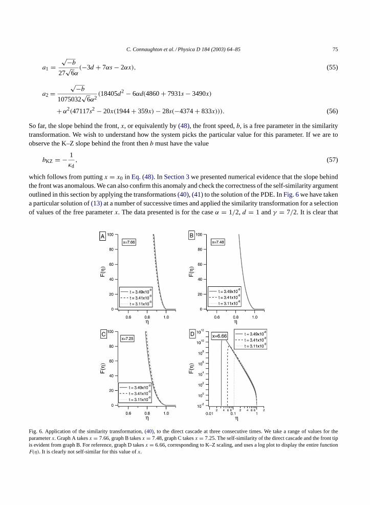
which follows from puttingx = x0 in Eq. (48). In Section 3we presented numerical evidence that the slope behindthe front was anomalous. We can also confirm this anomaly and check the correctness of the self-similarity argumentoutlined in this section by applying the transformations(40), (41)to the solution of the PDE. InFig. 6we have takena particular solution of(13)at a number of successive times and applied the similarity transformation for a selectionof values of the free parameterx. The data presented is for the caseα = 1/2, d = 1 andγ = 7/2. It is clear that
Fig. 6. Application of the similarity transformation,(40), to the direct cascade at three consecutive times. We take a range of values for theparameterx. Graph A takesx = 7.66, graph B takesx = 7.48, graph C takesx = 7.25. The self-similarity of the direct cascade and the front tipis evident from graph B. For reference, graph D takesx = 6.66, corresponding to K–Z scaling, and uses a log plot to display the entire functionF(η). It is clearly not self-similar for this value ofx.
76 C. Connaughton et al. / Physica D 184 (2003) 64–85
the direct cascade is self-similar forx = 7.48 approximately. This is to be compared with the theoretical predictionxc = 7.56. The corresponding transformation with K–Z value,x = 6.66 in this case, is clearly not self-similar.
The behaviour of the solution of the equation for the spectrum after the singular time,t∗, is an interestingquestion. Let us consider what could be called the “bouncing back” of the spectrum from infinity aftert = t∗.Our considerations are inspired by[9]. Exactly att = t∗ the spectrum becomes a pure power law,ω−xc, at largefrequencies. This can be understood as follows: any finite value ofω, however, large is in the wake part of theself-similar solution whent = t∗. This wake is a pure power spectrum. Therefore, att = t∗, we have a well-definedinitial condition for the evolution equation.
This spectrum is not a stationary solution (neither K–Z nor equilibrium) of the evolution equation. The subsequentevolution should follow the same principles as just beforet = t∗: the large frequency part of the spectrum has atypical timescale which goes to zero asω → ∞. This timescale is the timescale for relaxation to a stationary K–Zspectrum with constant energy flux. Although the amplitude of this spectrum itself changes in the course of time, itdoes so more and more slowly aftert = t∗ so that the changes induced in the K–Z spectrum by the change of energyflux become adiabatic relative to the infinitely short timescale for the large frequency evolution. This justifiesour consideration of the large time spectrum as a K–Z spectrum although it is not strictly speaking stationaryin time.
Let us assume now that the bouncing back of the K–Z spectrum from infinity is described by the same self-similarequation as beforet = t∗. One boundary condition is now different. The support of the self-similar spectrum nowgoes from zero to infinity and asω → ∞, nω ∼ ω−x0 with x0 being the K–Z exponent. Near small frequencieson this stretched scale, the spectrum keeps the same power behaviour as beforet = t∗ since the timescale there islong compared to the timescalet∗ − t at the high frequency end. We expect that arguments which we shall presentin Section A are relevant here too, with the corresponding solution of the self-similar equation being unique andthe free parameter required to adjust the trajectory reaching the low frequency behaviour along the stable manifoldbeing the amplitude of the K–Z spectrum at infinity. The solution of the self-similar equation should then specifythe shape of the “bend” in the spectrum seen inFig. 4and its time evolution will be then given by the same scalingof the frequencies in the similarity representation of the dynamical equations as we used beforet = t∗. Some furtherwork will be required to make these statements more concrete.
5. Derivation of the anomalous spectrum from the critical front speed hypothesis
In this section we present a heuristic derivation of the formula(8) as promised in the introduction. The program isas follows. We first calculate the energy balance in the neighbourhood of the front tip. We will find that the conditionthat energy is conserved by the motion of the tip is equivalent to the condition,(45), that the solution be self-similar.Next we calculate the amount of energy,E(t1, t2), which enters the frequency interval [ω∗(t1), ω∗(t2)] immediatelybehind the tip in the time interval [t1, t2]. The critical front speed hypothesis is the following:the physical systemselects the unique value of the front speed such thatlim t2→t∗E(t1, t2) is finite and non-zero for allt1 < t∗.
The basic energy balance equation for the front tip is as follows:∫ t2
t1
∫ ω∗(t2)
ω∗(t1)
(∂E
∂t+ ∂P
∂ω
)dω dt = 0. (58)
This can be expanded to read∫ ω∗(t2)
ω∗(t1)(E(ω, t2)− E(ω, t1))dω = −
∫ t2
t1
(P(ω∗(t2), t)− P(ω∗(t1), t))dt. (59)
C. Connaughton et al. / Physica D 184 (2003) 64–85 77
We observe thatE(ω, t1) = 0 sinceω∗(t1) < ω andP(ω∗(t2), t) = 0 sinceω∗(t) < ω∗(t2). Hence we obtain thefundamental balance equation for the front tip,∫ ω∗(t2)
ω∗(t1)E(ω, t2)dω =
∫ t2
t1
P(ω∗(t1), t)dt. (60)
Let us now calculateP andE near the front tip using the expansion(53)but keeping only the leading order term:
F(η) = a0(1 − η)3/2 + O((1 − η)5/2).
In terms ofω andt,
n(ω, t) = a0ω∗(t)−x−3/2(ω∗(t)− ω)3/2 + O((ω∗(t)− ω)5/2).
We substitute this expression fornω(t) into Eqs. (24) and (23)and keep only the leading power ofω∗(t) − ω. Forthe energy, we obtain
E(ω, t) = Ωda0ω∗(t)−x−3/2ωd/α(ω∗(t)− ω)3/2 + O((ω∗(t)− ω)5/2). (61)
For the flux we obtain
P(ω, t) = 758 a
30ω
3x0+3ω∗(t)−3x−9/2(ω∗(t)− ω)3/2 + O((ω∗(t)− ω)5/2). (62)
In both these expressions we can write powers ofω asωy = (ω∗(t)− (ω∗(t)−ω))y and perform a Taylor expansionin (ω∗(t) − ω). Since we are keeping only terms to leading order in(ω∗(t) − ω), we can consistently replaceωy
with ω∗(t)y to yield the following expressions:
E(ω, t) = Ωda0ω∗(t)−x−3/2+d/α(ω∗(t)− ω)3/2 + O((ω∗(t)− ω)5/2), (63)
P(ω, t) = 758 a
30ω
∗(t)3(x0−x)−3/2(ω∗(t)− ω)3/2 + O((ω∗(t)− ω)5/2). (64)
We now substitute these expressions into(60) and perform the integrals to leading order. Let us first consider theLHS∫ ω∗(t2)
ω∗(t1)E(ω, t2)dω=Ωda0
∫ ω∗(t2)
ω∗(t1)ω∗(t2)−x−3/2+d/α(ω∗(t2)− ω)3/2 dω + h.o.t.
= 2
5Ωdω
∗(t2)−x−3/2+d/α(ω∗(t2)− ω∗(t1))5/2 + h.o.t. (65)
Now consider the RHS∫ t2
t1
P(ω∗(t1), t)dt = 75
8a3
0
∫ t2
t1
ω∗(t)3(x0−x)−3/2(ω∗(t)− ω∗(t1))3/2 dt + h.o.t.
Let us change integration variablest → ω∗(t):∫ t2
t1
P(ω∗(t1), t)dt = 75
8a3
0
∫ ω∗(t2)
ω∗(t1)ω∗(t)3(x0−x)−3/2(ω∗(t)− ω∗(t1))3/2
(dω∗
dt
)−1
dω∗ + h.o.t.
We now use the self-similarity condition,(45), to express the derivative in terms ofω∗(t) and perform the Taylorexpansion trick again: for some power,y, we write:ω∗(t)y = (ω∗(t1) + (ω∗(t) − ω∗(t1)))y = ω∗(t1)y + h.o.t.
78 C. Connaughton et al. / Physica D 184 (2003) 64–85
This gives∫ t2
t1
P(ω∗(t1), t)dt = 75
8a3
0ω∗(t1)3(x0−x)−3/2ω∗(t1)−(3x0−2x−d/α)
∫ ω∗(t2)
ω∗(t1)(ω∗ − ω)3/2 dω∗ + h.o.t.,
∫ t2
t1
P(ω∗(t1), t)dt = 75
8a3
0ω∗(t1)3(x0−x)−3/2
(dω∗
dt1
)−1 2
5(ω∗(t2)− ω∗(t1))5/2 + h.o.t. (66)
Equating(65) and (66)and lettingt1 → t2, we obtain energy balance criterion
dω∗
dtω∗2x−3x0+d/α = 1 (67)
which is equivalent to the self-similarity condition that(45)be time independent.Now suppose we taket2 − t1 to be small but finite and allowt2 → t∗. It is clear that the energy flux,(66), entering
the region [ω∗(t1), ω∗(t2)] in this last increment of time before the front reaches infinity is either infinite, a finitequantity, or zero. Our hypothesis is that the flux is finite. It certainly cannot be infinite since the entire system hasfinite energy. It seems unreasonable that it should be zero since the front presumably requires a supply of energyto continue moving. A finite value for the integrated flux requires that the power ofω(t2) in (65) is zero. Thishypothesis leads to a unique value for the slope, which we shall denote byxc. From(65)
2
5Ωdω
∗(t2)−x−3/2+d/α(ω∗(t2)−ω∗(t1))5/2+h.o.t.=Ωdω∗(t2)−x−3/2+d/α
(dω∗
dt2
)5/2 2
5(t2 − t1)
5/2 + h.o.t.
(68)
2
5Ωdω
∗(t2)−x−3/2+d/α(ω∗(t2)− ω∗(t1))5/2 + h.o.t.=ω∗(t2)−6(x−x0−((2γ−3α)/12α))Ωd
2
5(t2 − t1)
5/2 + h.o.t.
(69)
In order that this remain finite but non-zero asω∗(t2) → ∞, we require
x = xc = x0 + 2γ − 3α
12α. (70)
The physical intuition behind this hypothesis is the following. Ifx > xc, the front speed is slower than the criticalvalue. The power in(69)is positive and the energy in the tip diverges asω∗(t2) → ∞. The front is moving too slowlyfor the amount of flux flowing into it so that energy begins to pile up at the tip. On the other hand, ifx < xc, the frontmoves faster than the critical value. Then energy in the tip decays to zero asω∗(t2) → ∞ which means that thefront is moving too fast for the amount of energy supplied to it. Physically we expect that the former situation wouldtend to speed up the front and the latter would tend to slow it down thus providing the system with a self-regulatorymechanism which selects the marginal slope,xc.
6. Concluding remarks
From the work presented here, we are beginning to get a clearer understanding of how the K–Z spectrum is set upin this model and the origins of the anomalous spectrum in the wake. The most obvious and important question whichwe have not addressed at all here is that of whether any of this analysis is relevant for the full kineticequation (1).It seems unlikely that the detailed structure of the nonlinear front would carry over to the integral version of thekinetic equation. Indeed, it is difficult to see how a sharp front tip could co-exist with thek-space integrations onthe RHS of(1).
C. Connaughton et al. / Physica D 184 (2003) 64–85 79
Nevertheless, anomalous behaviour has been observed[6] in numerical simulations of the full three-wave kineticequation as already mentioned. This gives us reason to hope that some of the qualitative ideas contained here canbe extended to more general kinetic equations. In particular, if the dynamics of the front is indeed regulated by acritical speed hypothesis of the type proposed inSection 5, then there is hope that an analogue can be formulatedeven in the absence of a sharp tip.
One might also speculate that this mechanism might occur in the evolution of the Kolmogorov spectrum ofhydrodynamic turbulence since the direct cascade in this case is also of finite energy capacity. Unfortunately, inthe absence of a closed kinetic equation for hydrodynamic turbulence it is not clear how one would even beginto address this question from a mathematical point of view. Nevertheless, for the purpose of stimulating debate,let us make the following conjecture. In far from equilibrium situations with stationary states which have finitecapacity, the evolution towards the stationary spectrum takes place in two stages. In the first stage, 0< t < t∗,which is rapid, the system attempts to close the connection with the dissipative sink at very high (or very low)wavenumbers. In that stage, entropy production is positive as the system attempts to explore all the available phasespace subject to the constraint of energy conservation. The wake spectrum is steeper (shallower if the sink is atk = 0) than that of the final stationary state. This slope is determined by the requirement that a finite amountof energy per unit time is delivered to the front tip at all times less thatt∗. After t = t∗, energy is no longerconserved but entropy production is still positive as the system now explores a larger volume of phase space.However, the entropy production now decreases as a new front with the K–Z spectrum in its wake (between thefront andk = ∞) moves towards lower wavenumbers and invades the steeper spectrum set up during the firststage of evolution. While it may be difficult to confirm these conjectures in a quantitative manner for the varietyof situations to which we suggest these ideas apply, it should not be too difficult to establish them (or prove themincorrect) qualitatively.
Acknowledgements
The authors would like to thank Oleg Zaboronski and Sergey Nazarenko for numerous helpful discussions. CCand ACN would like to acknowledge the hospitality of the Erwin Schrodinger Institute during the 2002 Programon Developed Turbulence. We are grateful for financial support from NSF Grant 0072803, the EPSRC and theUniversity of Warwick.
Appendix A. Analysis of the self-similarity equation and the critical front speed
Here we shall analyse the similarityequation (44)further. We wish to check that it does indeed admit solutionswhich reproduce the critical behaviour which we have ascribed to the solutions of its antecedent PDE inSection 5.Specifically, we are interested in solutions which match theF(η) ∼ (1 − η)3/2 singularity atη = 1 to a power lawsolution,F(η) ∼ η−x asη → 0.
Let us write(44) in the form
η−1+d/α(
xF + η∂F
∂η
)= (2(x− x0)− κd)
d2
dη2
(ηsF4 d2
dη2
(1
F
))(A.1)
and look for solutions of the formF(η) = Aη−y. Substituting this form we obtain
(−y + x)η(d/α)−1−y = 3A2y(y − 1)(x0 − y)(3x0 − 3y − 1)(2(x− x0)− κd)η3x0−3y−2. (A.2)
80 C. Connaughton et al. / Physica D 184 (2003) 64–85
We see that we can have the following solutionsy = x wherex takes one of the following values:
x = 0, (A.3)
x = 1, (A.4)
x = x0, (A.5)
x = x0 − 13. (A.6)
The first pair are the thermodynamic spectra, the second pair are the K–Z energy and particle spectra, respectively.A fifth special value ofy is
x = x0 + 12κd. (A.7)
What we observe from numerical solution of the ODE(A.1), described below, is as follows. If we choose a valueof x which is notxc = x0 + κd/4, then the solution,η−x, makes a transition nearη = 0 to the stateη−y, wherey = x0 + κd/2. This behaviour nearη = 0 balances the leading order divergences on both sides ofEq. (A.1)asη → 0. It might be noted, although it may have no relevance to the problem under consideration, that this value forthe exponent,y, leads to front dynamics,ω∗(t) = (t∗ − t)b with zerob. This spectrum was never observed in thesolutions of the PDE.
To find solutions of(44) which do not exhibit thex0 + κd/2 scaling asη → 0, we decided to perform a set ofnumerical experiments. Let us write out the RHS explicitly so that we can see exactly the equation which we wishto solve:
1
2(x− x0)− κdη−1+(d/α)
(xF + η
dF
dη
)= −ηsF2 d4F
dη4− 2sηs−1F2 d3F
dη3+ 2ηsF
(d2F
dη2
)2
+ 8ηs(
dF
dη
)d2F
dη2+ 4sηs−1
(dF
dη
)3
+ 4sηs−1FdF
dη
d2F
dη2
+ 2s(s− 1)ηs−2F
(dF
dη
)− s(s− 1)ηs−2F2 d2F
dη2. (A.8)
The problem with integrating(A.8) on a computer is that for generic initial conditions, the strong power lawdependences of the RHS on the independent variable render the numerics very susceptible to round-off error andnumerical instability. For example, to study the system withγ = 7/2, α = 1/2, d = 1, to which we gave a lot ofconsideration inSection 3due to its relatively large anomaly, we are required to take 3x0 + 2 = 22.
To get around this difficulty, and to aid visualisation of the global properties of the equation, we make the followingchange of variables:
F(η) = ηaf(τ),dF
dη= ηa−1g(τ),
d2F
dη2= ηa−2h(τ),
d3F
dη3= ηa−3k(τ), (A.9)
whereτ = log(η). By choosing
a = 1
2
(d
α− s+ 3
)= −x0 − κd
2, (A.10)
C. Connaughton et al. / Physica D 184 (2003) 64–85 81
we can cancel all the power dependence from the system and eventually recast(A.8) as the following autonomousfourth-order system:
df
dτ= g− af,
dg
dτ= h− (a− 1)g,
dh
dτ= k − (a− 2)h,
f 2 dk
dτ= − 1
2(x− x0)− κd(g+ xf)− (a+ 2s− 3)f 2k + 2fh2 + 8g2h+ 4sg3 + 4sfgh
+ 2s(s− 1)fg2 − s(s− 1)f 2h. (A.11)
Only the region,f ≥ 0 makes physical sense sincenω, and henceF , cannot be negative. This system is singular onthe hyperplanef = 0. This system is much easier to integrate numerically and has the added advantage that we candetermine the presence of fixed points which are not obvious in the original differential equation. Let us determinethese points. It is obvious that the RHS of(A.11)has a trivial zero at(f, g, h, k) = (0,0,0,0) = O but this is clearlya singular point due to the factor off 2 on the LHS. A second pair of non-trivial (and non-singular) fixed points canbe shown after quite a bit of algebra to exist at the pointsP± = (f0,af0, a(a− 1)f0, a(a− 1)(a− 2)f0), where
f0 = ±(18a(a+ 1)(a+ 13(s− 2))(a+ 1
3(s− 3)))−1/2. (A.12)
We are naturally only interested in the pointP+ sinceP− lies in the negativef region. The factors(a+ (s− 2)/3)and(a+ (s− 3)/3) are interesting for the following reason. If we substitute back ins = 3x0 + 2 and the value ofafrom (A.10), these two factors are simply−κd/2 and−κi/2, respectively. At the transition points between finite andinfinite capacity the fixed point runs away to infinity which suggests that it has a central role to play in organisingthe critical solution in the finite capacity case.
Let us now look for a numerical solution of this system which mirrors the solutions of the differential kineticequation. All the simulations in this section were done using the transformed system,(A.11), for which a standardout-of-the-box adaptive Runge–Kutta routine seemed to work fine. Suppose we want a solution for the wake of theform F(η) ∼ η−x asη → 0. In the new variables this is equivalent to demanding
f(η) ∼ Aη−a−x, g(η) ∼ −xf(η), h(η) ∼ x(x+ 1)f(η), k(η) ∼ −x(x+ 1)(x+ 2)f(η)
asη → 0 or asτ → −∞. If x < −a = x0 + κd/2, which is the case, then we observe that the wake is describedby a trajectory for which(f, g, h, k) → (0,0,0,0) asτ → −∞. The wake is the singular point,O, of the system,(A.11). As we approachη → 1 we must reproduce the front structure described inSection 4. Thus we require atrajectory for which(f, g, h, k) → F asτ → 0, whereF = (0,0,∞,∞). We require a trajectory which links thesetwo singular points.
In our numerical simulations we rescaled the variables as follows:
f → f
f0, g → g
af0, h → h
a(a− 1)f0, k → k
a(a− 1)(a− 2)f0.
This maps the pointP+ → (1,1,1,1) for ease of visualisation. The only difference is that sincea < 0, the signs ofg andk are swapped so that the wake part of the solution must now approachO from the direction(0+,0+,0+,0+)and the front tip,F , is now at(0+,0+,∞,−∞).
It turns out to be difficult to find a trajectory linkingF → O. We performed a series of experiments integratingbackwards from 1− η = ε, with ε 1, towardsη = 0. Because we cannot specify initial data exactly at thesingular point,F , we were required to manually tune the initial conditions quite a bit in order to reproduce theF(η) ∼ (1− η)3/2 structure near the tip. The remaining adjustable parameter in the equation isx. We again chooseto study the caseγ = 7/2, α = 1/2, d = 1. Two generic types of trajectory emerge as we varyx. We visualise
82 C. Connaughton et al. / Physica D 184 (2003) 64–85
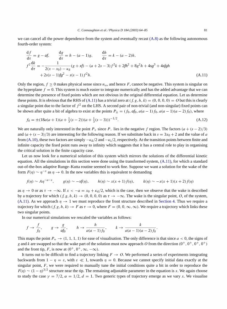
Fig. 7. Trajectory in(f, g, h, k) space forx = 7.56275, which is less than the critical value.
these trajectories in four-dimensional phase space as a pair of projections of the actual trajectory onto the(f, g) and(h, k) planes, respectively, hence the apparent intersections.
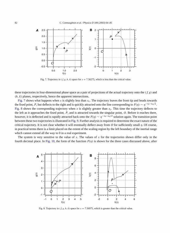
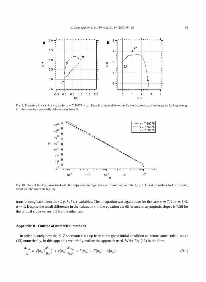
Fig. 7shows what happens whenx is slightly less thanxc. The trajectory leaves the front tip and heads towardsthe fixed point,P , but deflects to the right and is quickly attracted onto the line corresponding toF(η) ∼ η−x0−κd/2.Fig. 8 shows the corresponding trajectory whenx is slightly greater thanxc. This time the trajectory deflects tothe left as it approaches the fixed point,P , and is attracted towards the singular point,O. Before it reaches there,however, it is deflected and is rapidly attracted back onto theF(η) ∼ η−x0−κd/2 solution again. The transition pointbetween these two trajectories is illustrated inFig. 9. Further analysis is required to determine the exact nature of thecritical trajectory. It is not clear whether it will eventually deflect away fromO for sufficiently smallη. Of course,in practical terms there is a limit placed on the extent of the scaling region by the left boundary of the inertial rangewhich cannot extend all the way to 0 in a real experiment.
The system is very sensitive to the value ofx. The values ofx for the trajectories shown differ only in thefourth decimal place. InFig. 10, the form of the functionF(η) is shown for the three cases discussed above, after
Fig. 8. Trajectory in(f, g, h, k) space forx = 7.56975, which is greater than the critical value.
C. Connaughton et al. / Physica D 184 (2003) 64–85 83
Fig. 9. Trajectory in(f, g, h, k) space forx = 7.56875≈ xc. Since it is impossible to specify the data exactly, if we integrate for long enoughin τ this trajectory eventually deflects away fromO.
Fig. 10. Plots of theF(η) associated with the trajectories inFigs. 7–9after converting from the(f, g, h, k) andτ variables back toF andηvariables. The scales are log–log.
transforming back from the(f, g, h, k), τ variables. The integration was again done for the caseγ = 7/2,α = 1/2,d = 1. Despite the small difference in the values ofx in the equation the difference in asymptotic slopes is 7.56 forthe critical slope versus 8.5 for the other two.
Appendix B. Outline of numerical methods
In order to study how the K–Z spectrum is set up from some given initial condition we wrote some code to solve(13)numerically. In this appendix we briefly outline the approach used. WriteEq. (13)in the form
∂nω
∂t= f [nω]
∂4nω
∂ω4+ g[nω]
∂3nω
∂ω3+ h[nω] + F [nω] − ν[nω], (B.1)
84 C. Connaughton et al. / Physica D 184 (2003) 64–85
where
f [nω] = −Λ−1ω ωsn2, (B.2)
g[nω] = −2Λ−1ω sωs−1n2, (B.3)
h[nω] = Λ−1ω
ωs
(2n
(∂2n
∂ω2
)2
+ 8
(∂n
∂ω
)2∂2n
∂ω2
)+ 2sωs−1
(2
(∂n
∂ω
)3
+ 2n∂n
∂ω
∂2n
∂ω2
)
+ s(s− 1)ωs−2
(2n
(∂n
∂ω
)2
− n2 ∂2n
∂ω2
), (B.4)
Λω = Ωk
αω(d/α)−1, (B.5)
s = 3x0 + 2. (B.6)
We are now including forcing and damping terms,F [nω] and ν[nω] which can be chosen as appropriate. Weperformed the following implicit time discretisation,
nω(t +2t)− nω(t)
2t= f [nω(t)]
∂4nω(t +2t)
∂ω4+ g[nω(t)]
∂3nω(t +2t)
∂ω3+ h[nω(t)]
+F [nω(t +2t)] − ν[nω(t +2t)] (B.7)
with the aim of enhancing the stability of the higher order derivatives. This can be rearranged to yield a time steppingalgorithm in the form
nω(t +2t) = L−1[nω(t)]B[nω(t)], (B.8)
where
L[nω] = 1 +2t f [nω]∂4
∂ω4+2t g[nω]
∂3
∂ω3(B.9)
B[nω] = nω +2t h[nω] +2t F [nω]. (B.10)
The time evolution operator,L[nω], and source,B[nω], are approximated using centred difference representationsfor the derivatives and a standard linear solver used to perform the inversion at each time-step. Implementingconsistent boundary conditions is a tricky task. For all of the simulations presented here, the equation was solvedfrom a compactly supported initial condition either in a frequency interval sufficiently large that the solution doesnot reach the boundary within the time allotted or with the damping chosen sufficiently strong to prevent the solutionfrom ever reaching the boundary.
Most of the simulations presented here are of a freely decaying initial energy distribution soF [nω] = 0. Thedamping was chosen to be zero over most of the interval but increasing strongly forω < ωL andω > ωR to produceregions of strong dissipation at large and small scales. We typically used approximately 10 grid points per unitfrequency interval in our discretisation. The simulations presented here used up to 20,000 grid-points. The numberof grid points is practically limited by the fact that one must recompute and invert the time evolution operator,(B.9),at each time-step. Lacking any reliable stability criteria for the nonlinear discretisation scheme described above,the choice of time-step was essentially made by trial and error. Once a time-step was found for which the evolutionseemed stable, we ran with it. We were aided in choosing this time-step by monitoring the two conservation lawsassociated with the total energy and total particle number. Typically, and unsurprisingly, the numerics become
C. Connaughton et al. / Physica D 184 (2003) 64–85 85
unstable most easily at the front tip. This instability is worse for steeper spectra when the front travels faster. Thenecessity of reducing the time-step to resolve this structure as the tip increases in speed also put practical limits onthe time interval we could simulate for. Retrospectively, we would like to do the numerics using an adaptive gridwhich tracks the front. Such a method would probably yield great increases in efficiency and stability. Unfortunatelyat the outset, we did not really appreciate that the code would be required to tackle this problem. We settled forvalidating our computations by checking that our final results remained unchanged when the time-step was reducedby a factor of 2.
References
[1] A.A. Lacey, J.R. Ockendon, A.B. Tayler, Waiting time solutions of a nonlinear diffusion equation, SIAM J. Appl. Math. 42 (6) (1982)1252–1264.
[2] P.J. Aucoin, A.C. Newell, Semidispersive wave systems, J. Fluid Mech. 49 (1971) 593–609.[3] D.J. Benney, A.C. Newell, Sequential time closures of interacting random waves, J. Math. Phys. 46 (1967) 363.[4] S. Dyachenko, A.C. Newell, A. Pushkarev, V.E. Zakharov, Optical turbulence: weak turbulence, condensates and collapsing filaments in
the nonlinear Schrodinger equation, Physica D 57 (1992) 96–160.[5] G.E. Falkovich, A.V. Shafarenko, Non-stationary wave turbulence, J. Nonlinear Sci. 1 (1991) 452–480.[6] S. Galtier, S.V. Nazarenko, A.C. Newell, A. Pouquet, A weak turbulence theory for incompressible MHD, J. Plasma Phys. 63 (2000)
447–488.[7] K. Hasselmann, On the nonlinear energy transfer in a gravity wave spectrum I, J. Fluid Mech. 12 (1962) 481–500.[8] K. Hasselmann, On the nonlinear energy transfer in a gravity wave spectrum II, J. Fluid Mech. 15 (1963) 273–281.[9] R. Lacaze, P. Lallemand, Y. Pomeau, S. Rica, Dynamical formation of a Bose–Einstein condensate, Physica D 152–153 (2001) 779–786.
[10] A.C. Newell, P.J. Aucoin, Semidispersive wave systems, J. Fluid Mech. 49 (1971) 593–609.[11] A.C. Newell, S. Nazarenko, L. Biven, Wave turbulence and intermittency, Physica D 152–153 (2001) 520–550.[12] C.S. Ng, A. Bhattachargee, Interaction of shear Alfven wave packets: implication for weak magnetohydrodynamic turbulence in
astrophysical plasmas, Astrophys. J. 465 (2) (1996) 845–854.[13] V.E. Zakharov, N. Filonenko, The energy spectrum for stochastic oscillation of the fluid surface, Doklady Akad. Nauk SSSR 170 (1966)
1292–1295.[14] V.E. Zakharov, R.Z. Sagdeev, On spectra of acoustic turbulence, Dokl. Akad. Nauk SSSR 192 (2) (1970) 297–299 (English Trans.: Soviet
Phys. JETP 35 (1972) 310–314).[15] V.S. Zakharov, V.S. Lvov, G. Falkovich, Kolmogorov Spectra of Turbulence, Springer, Berlin, 1992.[16] Y.B. Zel’dovich, A.S. Kompaneets, On the theory of heat propagation for temperature dependent thermal conductivity, in: Collection
Commemorating the 70th Anniversary of A.F. Joffe. Izdat. Akad. Nauk SSSR, Moscow, 1950.