Embed Size (px)
Citation preview

NON-TECHNICAL LOSS FRAUD
DETECTION IN
SMART GRID
by
WENLIN HAN
YANG XIAO, COMMITTEE CHAIRXIAOYAN HONGSUSAN VRBSKY
JINGYUAN ZHANGO’NEILL ZHENG
A DISSERTATION
Submitted in partial fulfillment of the requirementsfor the degree of Doctor of Philosophyin the Department of Computer Science
in the Graduate School ofThe University of Alabama
TUSCALOOSA, ALABAMA
2017

Copyright Wenlin Han 2017ALL RIGHTS RESERVED

ABSTRACT
Utility companies consistently suffer from the harassing of Non-Technical Loss
(NTL) frauds globally. In the traditional power grid, electricity theft is the main form of
NTL frauds. In Smart Grid, smart meter thwarts electricity theft in some ways but cause
more problems, e.g., intrusions, hacking, and malicious manipulation. Various detectors
have been proposed to detect NTL hhfrauds including physical methods,
intrusion-detection based methods, profile-based methods, statistic methods and
comparison-based methods. However, these methods either rely on user behavior analysis
which requires a large amount of detailed energy consumption data causing privacy
concerns or need a lot of extra devices which are expensive. Or they have some other
problems. In this dissertation, we thoroughly study NTL frauds in Smart Grid. We
thoroughly survey the existing solutions and divided them into five categories. After
studying the problems of the existing solutions, We propose three novel detectors to detect
NTL frauds in Smart Grid which can address the problems of all the existing solutions.
These detectors model an adversary’s behavior and detect NTL frauds based on several
numerical analysis methods which are lightweight and non-traditional. The first detector is
named NTL Fraud Detection (NFD) which is based on Lagrange polynomial. NFD can
detect a single tampered meter as well as multiple tampered meters in a group. The second
detector is based on Recursive Least Square (RLS), which is named Fast NTL Fraud
Detection (FNFD). FNFD is proposed to improve the detection speed of NFD. Colluded
NTL Fraud Detection (CNFD) is the third detector that we propose to detect colluded
NTL frauds. We have also studied the parameter selection and performance of these
detectors.
ii

DEDICATION
I dedicate my Ph.D dissertation to my supervisor, Dr. Yang Xiao, and other
dissertation committee members, Dr. Xiaoyan Hong, Dr. Susan Vrbsky, Dr. Jingyuan
Zhang and Dr. O’neill Zheng. Their support was to different extents and along with many
other persons crucial for the completion of my dissertation.
I would like to express my deepest gratitude to the dean, Dr. David Cordes, and
other faculty and staff in Computer Science department who offered collegial guidance and
support over the years.
I would like to extend my thanks to my family and the many friends who supported
me on this journey.
iii

LIST OF ABBREVIATIONS AND SYMBOLS
A The array of all coefficients
Aj The estimation of A after j times of measurements
αi,j The accuracy ratio of Meter i during Tj
αmax The upper limit of the accuracy ratio of Meter i during Tj
αmin The lower limit of the accuracy ratio of Meter i during Tj
AMI Advanced Metering Infrastructure
CNFD Colluded NTL Fraud Detection
e The user defined error
Ei,j The unit of electricity consumed by a consumer i during Tj
Ej The total unit of electricity recorded by the observer meter in Tj
ET The matrix of Ej
FNFD Fast NTL Fraud Detection
I The identity matrix
i The numbering of meters
IDS Intrusion Detection Systems
j The numbering of time intervals
k A constant with a high value
λ A forgetting factor which has a value between 0 and 1
m The order of the Lagrange polynomial
mmax The maximum order of the Lagrange polynomial
N The total number of meters in a community
iv

n The number of meters in one observation group
NCG Non-cooperative Game
NFD NTL Fraud Detection
NTL Non-Technical Loss
o The number of the observer meters installed in a community
OPF Optimum-Path Forest
P The degree of precision of the measurement
PLC Power Line Carrier
ri,j The distance from a point to the closest line of Meter i in Tj
RLS Recursive Least Square
S The summation of the distances rij
SCADA Supervisory Control and Data Acquisition System
Tj The measured time intervals
W The array of weight
w1 The weight of the detection time
w2 The weight of the number of the observer meters
X The matrix of xi,j
xi,j The unit of billed electricity, which is recorded by Meter i during Tj
v

ACKNOWLEDGMENTS
This work was partially supported by the National Science Foundation (NSF) under
grant CNS-1059265.
vi

vii
CONTENTS
ABSTRACT ………………………………………………………………………………… ii
DEDICATION ……………………………………………………………………………… iii
LIST OF ABBREVIATIONS AND SYMBOLS …………………………………………… iv
ACKNOWLEDGMENTS ………………………………………………………………….. vi
LIST OF TABLES …………………………………………………………………………… x
LIST OF FIGURES ………………………………………………………………………… xii
CHAPTER 1 INTRODUCTION …………………………………………………………… 1
CHAPTER 2 BACKGROUND AND LITERATURE REVIEW ………………………….. 5
2.1 Background ................................................................................................................... 5
2.2 Non-Technical Loss Fraud ............................................................................................ 7
2.3 Problem Definition and Attack Model.......................................................................... 8
2.4 Literature Review........................................................................................................... 9
2.4.1 Physical Method ............................................................................................... 9
2.4.2 IDS-based Method ........................................................................................... 10
2.4.3 Profile-based Method........................................................................................ 11
2.4.4 Comparison-based Method............................................................................... 11
2.4.5 Statistic Method ............................................................................................... 12
CHAPTER 3 NFD: NTL FRAUD DETECTION ……………………………………………. 13
3.1 Introduction................................................................................................................... 13
3.2 Working Process and Algorithm................................................................................... 14

viii
3.3 Experiments................................................................................................................. 21
3.3.1 Experiment 1: No Tampered Meters ................................................................. 22
3.3.2 Experiment 2: Single Adversary and Single Tampered Meter.......................... 23
3.3.3 Experiment 3: Multiple Adversaries and Multiple Tampered Meters………… 25
3.4 Parameter Selection and Discussion.............................................................................. 28
3.4.1 Error and Selection of Order m ........................................................................ 28
3.4.2 Detection Time and Selection of User Number n............................................. 34
3.5 Conclusion.................................................................................................................... 36
CHAPTER 4 FNFD: FAST NTL FRAUD DETECTION AND VERIFICATION ………… 37
4.1 Introduction................................................................................................................... 37
4.2 Working Process and Algorithm................................................................................... 37
4.3 Experiments.................................................................................................................. 42
4.3.1 Detect a Single Tampered Meter ..................................................................... 42
4.3.2 Detect Multiple Tampered Meters.................................................................... 43
4.3.3 Detect All Tampered Meters............................................................................. 46
4.4 Performance Comparison............................................................................................ 47
4.4.1 Fraud Detection................................................................................................. 48
4.4.2 Fraud Verification............................................................................................. 49
4.5 Parameter Tuning.......................................................................................................... 51
4.5.1 Tuning k ............................................................................................................ 51
4.5.2 Tuning λ ........................................................................................................... 51
4.5.3 Tuning A0 ......................................................................................................... 52
4.5.4 Tuning n ........................................................................................................... 54

ix
4.6 FNFD Stability and Convergence ................................................................................ 56
4.6.1 FNFD Stability................................................................................................... 56
4.6.2 FNFD Convergence........................................................................................... 57
4.7 Conclusion................................................................................................................... 60
CHAPTER 5 CNFD: COLLUDED NTL FRAUD DETECTION …………………………. 61
5.1 Introduction.................................................................................................................. 61
5.2 Colluded NTL Fraud.................................................................................................... 62
5.3 CNTL Fraud Detection................................................................................................ 64
5.3.1 Observer Meter................................................................................................ 64
5.3.2 Tampered Meter Detection............................................................................. 65
5.3.3 Fraudster Differentiation................................................................................. 68
5.4 Experiments................................................................................................................ 70
5.4.1 Experiment 1: Segmented CNTL .................................................................... 70
5.4.2 Experiment 2: Fully Overlapped CNTL.......................................................... 72
5.4.3 Experiment 3: Partially Overlapped CNTL..................................................... 72
5.4.4 Experiment 4: Combined CNTL...................................................................... 75
5.5 Conclusion................................................................................................................... 77
CHAPTER 6 CONCLUSION ……………………………………………………………… 79
REFERENCES …………………………………………………………………………….. 80
APPENDIX A PROOF OF THEOREM 3.1 ………………………………………………… 87

LIST OF TABLES
3.1 The unit of the billed electricity in NFD - Exp. 1 . . . . . . . . . . . . . . . 22
3.2 Experimental results of NFD. . . . . . . . . . . . . . . . . . . . . . . . . . . 23
3.3 The unit of the billed electricity in NFD - Exp. 2 . . . . . . . . . . . . . . . 24
3.4 The unit of the billed electricity in NFD - Exp. 3 . . . . . . . . . . . . . . . 25
3.5 Comparison of the accuracy magnitude . . . . . . . . . . . . . . . . . . . . . 32
4.1 The unit of the billed electricity in FNFD - Exp. 1 . . . . . . . . . . . . . . 43
4.2 The unit of the billed electricity in FNFD - Exp. 2 . . . . . . . . . . . . . . 45
4.3 The unit of the billed electricity in FNFD - Exp. 3 . . . . . . . . . . . . . . 46
5.1 The recorded electricity consumption (kWh) in CNFD - Exp. 1 . . . . . . . 73
5.2 The recorded electricity consumption (kWh) in CNFD - Exp. 2 . . . . . . . 75
5.3 The recorded electricity consumption (kWh) in CNFD - Exp. 3 . . . . . . . 77
5.4 The recorded electricity consumption (kWh) in CNFD - Exp. 4 . . . . . . . 78
x

LIST OF FIGURES
2.1 The conceptual communication framework of AMI. . . . . . . . . . . . . . . 6
2.2 The conceptual framework of NTL fraud. . . . . . . . . . . . . . . . . . . . . 9
3.1 Install an observer meter. . . . . . . . . . . . . . . . . . . . . . . . . . . . . 15
3.2 NFD: mathematical models of the tampered meters and the normal meters. . 17
3.3 The experimental results of NFD - Exp. 2. . . . . . . . . . . . . . . . . . . . 26
3.4 The experimental results of NFD - Exp. 3. . . . . . . . . . . . . . . . . . . . 27
3.5 The experimental results of NFD - lowering order. . . . . . . . . . . . . . . . 29
3.6 The experimental results of NFD - error comparision. . . . . . . . . . . . . . 30
4.1 Mathematical models of normal and abnormal meters in FNFD. . . . . . . . 39
4.2 The coefficient converging process of FNFD in Exp.1. . . . . . . . . . . . . . 44
4.3 The coefficient converging process of FNFD in Exp.2. . . . . . . . . . . . . . 44
4.4 The coefficient converging process of FNFD in Exp.3. . . . . . . . . . . . . . 47
4.5 FNFD: fraud detection speed comparison. . . . . . . . . . . . . . . . . . . . 48
4.6 FNFD: data needed comparison in fraud detection. . . . . . . . . . . . . . . 49
4.7 FNFD: fraud verification speed comparison. . . . . . . . . . . . . . . . . . . 50
4.8 FNFD: data needed comparison in fraud verification. . . . . . . . . . . . . . 50
4.9 Detection speed comparison with different values of k. . . . . . . . . . . . . . 52
4.10 Detection speed comparison with different values of λ. . . . . . . . . . . . . . 53
4.11 Detection speed comparison with different values of ai0. . . . . . . . . . . . . 53
4.12 Detection speed comparison with different values of n. . . . . . . . . . . . . . 56
5.1 Four different types of CNTL frauds that we discovered. . . . . . . . . . . . 63
5.2 Modeling the behavior of fraudsters in CNFD mathematically. . . . . . . . . 65
xi

5.3 The tampered meter detection process of CNFD in Exp. 1. . . . . . . . . . . 71
5.4 The final detection result of CNFD in Exp. 1. . . . . . . . . . . . . . . . . . 71
5.5 The tampered meter detection process of CNFD in Exp. 2. . . . . . . . . . . 72
5.6 The final detection result of CNFD in Exp. 2. . . . . . . . . . . . . . . . . . 72
5.7 The tampered meter detection process of CNFD in Exp. 3. . . . . . . . . . . 74
5.8 The final detection result of CNFD in Exp. 3. . . . . . . . . . . . . . . . . . 74
5.9 The result of the first step, tampered meter detection, of CNFD in Exp. 4. . 76
5.10 The result of CNFD after the second step, fraudster differentiation, in Exp. 4. 76
A.1 NFD: a counter example. . . . . . . . . . . . . . . . . . . . . . . . . . . . . . 90
xii

CHAPTER 1
INTRODUCTION
Smart Grid has the capability of two-way communication and two-way electricity
flow, and this could be utilized by an adversary to manipulate any smart meter. When a
smart meter is manipulated by an adversary to gain illegal benefit and cause economic loss
to the utility, a Non-Technical Loss (NTL) fraud occurs. The economic loss has been
caused by NTL frauds is huge. In developed countries, such as United State, the annual
loss is $6 billion [44]. In developing countries, the annual loss due to NTL frauds is $58.7
billion, which is reported in a study of the top 50 emerging market countries, published by
northeast group, llc in 2014 [6]. These countries, including China, India, etc., will invest
$168 billion to deal with NTL frauds and build reliable Smart Grid till 2034.
NTL frauds have existed for a long time in the power grids, not only in Smart Grid.
The main form of NTL frauds is “stealing electricity” in the traditional power grid [41].
The main methods are physical methods such as slowing down an analog meter by adding
sand into it. In Smart Grid, smart meters are digital meters with built-in programs to
process and store data. In the communication networks of Smart Grid, every device can
communicate with another device in the networks, and these devices include smart meters,
home appliances, substations, head-end devices, etc. The malicious behavior of adversaries
are extended from a single meter to all the devices and channels in the networks. Besides
interrupting measurement, adversaries have two more ways to commit NTL frauds:
tampering with meters and intruding networks. They can remotely manipulate a smart
meter or even multiple smart meters simultaneously. Or they can intercept the
communication networks and inject falsified data into messages. NTL frauds are not
attacks, but they have a close relationship with attacks, including message manipulation,
1

key spoofing, impersonation attack, etc., in Smart Grid. In the traditional power grid, an
NTL fraud may last for a few months or longer, since the physical method that it relies on
is not easily withdrawn. For example, it is easy to add sand into a meter, but not easy to
take it out. This feature gives plenty of time to the utility to investigate an NTL fraud
case. Nevertheless, NTL frauds are much faster, more flexible and more complicated in
Smart Grid, therefore this challenges the detection speed of the existing schemes.
Various schemes have been proposed to detect NTL frauds, and they can be divided
into physical methods, intrusion-detection based methods, profile-based methods, statistic
methods and comparison-based methods. Existing physical methods include video
survalliance, power line inspection, etc. [10, 47] and they are expensive and inefficient.
Typical methods based on user profile analysis include machine learning, data mining,
etc. [12, 14, 43]. They have to analyze large volumes of detailed energy consumption data.
Typical IDS [18, 45] in Smart Grid are not introduced to detect NTL frauds but to deal
with security issues in Smart Grid generally. In the existing comparison-based
methods [58, 59,61], they can detect NTL frauds with a small amount of data, but the
detection speed still needs improvement. Statistic methods [35, 40] suffer from high false
alarm rate caused by variations such as change of weather, new home appliances, etc.
In this dissertation, we will introduce three novel detectors that we proposed to
detect NTL frauds in Smart Grid, which are NFD [26,31], FNFD [28,29] and
CNFD [21,32]. NFD can detect NTL frauds with only a small amount of data and one
additional device. NFD is based on Lagrange polynomial to model an adversary’s
behaviors, and detect a tampered meter by comparing the difference between the results.
Different from the existing detectors, our detector knows adversaries better than
adversaries themselves. By building mathematical models of these adversaries, we can
predict their behaviors which they may not be aware of by themselves. NFD makes it
practical to detect NTL frauds both online and offline in Smart Grid. NFD can facilitate
real-world applications before Smart Grid is fully deployed since it can serve the traditional
2

power grid and Smart Grid simultaneously. Experimental results show the effectiveness of
NFD. It can detect multiple tampered meters and multiple adversaries, as well as a single
tampered meter and a single adversary. We also study how to tune the parameters used in
NFD to further guide its practical usage.
FNFD is a fast NTL fraud detector which is proposed to improve the detection
speed of NFD and the other existing detectors. FNFD is based on Recursive Least Square
(RLS) to model adversary behavior. Experimental results show that FNFD outperforms
the existing schemes regarding detection speed and overhead. Moreover, experimental
results and theoretical analysis of parameter selection are also provided. We further study
the stability and convergence of FNFD theoretically. The study shows that FNFD is always
convergent as a control method if and only if the input dataset is persistent exciting.
In the literature, many detection schemes have been proposed to detect NTL frauds.
However, some NTL frauds are far more complicated than what the existing schemes
expect. We recently discovered a new potential type of frauds, a variant of NTL frauds,
called Colluded Non-Technical Loss (CNTL) frauds in the Smart Grid. In a CNTL fraud,
multiple fraudsters can co-exist or collaborate to commit the fraud. The existing detection
schemes cannot detect CNTL frauds since these methods do not consider the co-existing or
collaborating fraudsters, and therefore cannot distinguish one from many fraudsters. In
this dissertation, we propose a CNTL fraud detector to detect CNTL frauds. The proposed
method can quickly detect a tampered meter based on RLS. After identifying the tampered
meter, the proposed scheme can detect different fraudsters using mathematical models.
The experiments show that the scheme is effective in detecting CNTL frauds.
The rest of the dissertation is organized as follows. In Chapter 2, we introduce
Smart Grid, the background of NTL fraud, and the existing solutions. In Chapter 3, we
introduce the first proposed detector, NFD, including the working process, algorithm,
experiments and parameter selection. We present the second proposed detector, FNFD, in
Chapter 4, which includes the idea and algorithm, as well as the experimental results and
3

discussion. We present the third detector, CNFD, in Chapter 5. Finally, we conclude the
dissertation in Chapter 6.
4

CHAPTER 2
BACKGROUND AND LITERATURE REVIEW
2.1 Background
The traditional power system distributes electricity from power generation plants to
the end consumers in one direction, which is inefficient and unreliable since it cannot
satisfy the increasing future demand and the system is lacking efficient monitoring and
quick response, easily resulting in power outages. As reported in the paper [48], the cost is
approximate 100 billion dollars each year for power outages in US traditional power
systems. Smart Grid provides two-way electricity flow and data communication. The
two-way electricity flow incorporates distributed renewable energy better, such as solar and
wind energy, which benefits both environmental protection and the mitigation of the
energy crisis [15]. The two-way data communication provides intensive system monitoring
and quick system recovery.
Advanced Metering Infrastructure (AMI) is an automatic pricing, metering and
billing infrastructure in Smart Grid which integrates with current state-of-the-art electronic
hardware devices and software systems. AMI employs devices including smart meters, relay
meters, collectors, charging spots, substations, head-end devices, etc. One or multiple
smart meters are installed for each household or business to record energy usage. Relay
meters are used to relay messages to other meters or the head-end devices. Collectors are
used to gather information in sub-networks. Substations are used to manage electricity
distribution and also play a role in managing communication. The head-end devices are
servers employed by the utility to communicate with all other devices in AMI.
5

Home Area Network
Smart Meter
Home Area Network
Smart Meter
Neighborhood Area Network
Collector
Head-end System
Wide Area Network
...
...
Home Area Network
Smart Meter
Home Area Network
Smart Meter
Neighborhood Area Network
Collector
...
S ar
Figure 2.1: The conceptual communication framework of AMI.
Communication in AMI is two way. A smart meter can communicate with any other
smart meters in AMI. Each two devices, e.g. smart meters, relay meters, collectors,
charging spots, substations, head-end devices, etc. can communicate with each other. As
shown in Fig. 2.1, a Home Area Network (HAN) forms when home appliances and smart
meters in a household join the AMI. In a community, a collector is installed to gather local
information, thus forming a Neighbourhood Area Network (NAN) [60,62]. When several
HANs are connected and report to the head-end systems, it is a Wide Area Network
(WAN). In the U.S., the utility employs ANSI C12 serials as the communication protocols
for AMI, including ANSI C12.18, 19, 21 and 22 [3].
2.2 Non-Technical Loss Fraud
However, the development of Smart Grid has been raising new security and privacy
challenges. Globally, utility companies consistently suffer from NTL frauds. As
reported [55], the non-technical loss even exceeds the technical loss in some countries and is
6

estimated as about 1% of the worldwide electricity consumption. Beside electricity theft,
the frauds where customers gain illegal benefit by tampering meters, intruding networks,
etc. are also NTL frauds. This silence crime disturbs the normal billing process of power
companies, causes money loss, and is a waste of people’s efforts on energy conservation.
Besides poverty and economy recession, the temptation of free service is another
motivation to steal electricity in underdeveloped, developing, and developed countries, not
only limited to the low-income population.
The economic loss has been caused by NTL frauds is huge. In developed countries,
such as United State, the annual loss is $6 billion [44]. In developing countries, the annual
loss due to NTL frauds is $58.7 billion, which is reported in a study of the top 50 emerging
market countries, published by northeast group, llc in 2014 [6]. These countries, including
China, India, etc., will invest $168 billion to deal with NTL frauds and build reliable Smart
Grid till 2034. As Forbes reported [52], Florida utilities lose millions each year, and
thousands of NTL frauds have been reported by Duke Energy.
In the traditional power grid, the utility relies on physical methods, such as checking
power lines periodically, to detect NTL frauds. In Smart Grid, the development of AMI
enables smart meters with the capability of two-way communications. The utility can
intensively monitor smart meters to detect NTL frauds remotely. Smart meters dwarf
electricity theft using some physical methods, such as bypassing. However, the two-way
communication extends adversaries’ malicious behavior from the meters to the whole
generation, transmission, and distribution process. As FBI reported [56], hacking smart
meters is extremely easy and NTL frauds occur in various new forms.
Moreover, privacy protection is another challenge to detect NTL frauds in Smart
Grid. Smart meters store energy usage information, and this information are distributed all
over the communication networks, which potentially expose customer habits and
behaviors [44]. In Smart Grid, the customers lose control over the information delivered to
the utility unconsciously. Novel schemes to identify NTL without worrying about privacy
7

are needed. Furthermore, even if customers are totally willing to provide their personal
data, there’s still five to ten years before AMI is fully deployed [5]. The utility must find
efficient ways to detect NTL frauds right now.
2.3 Problem Definition and Attack Model
A community has N households and charging stations in total, and N smart meters
are installed to record the consumption. As shown in Fig. 2.2, the relationship between
meters and households or charging stations is one-to-one, and meters are connected to the
same secondary distribution network. A utility company is responsible for supplying
electricity to this community. However, the utility company found that the total amount of
the billing electricity is always much smaller than the amount that it supplied to the
community. After having transformers, power lines and other devices examined, the utility
company eliminated technical loss. NTL frauds are highly suspected on some meters. The
objectives include identifying tampered meters, pinpointing the locations, and learning the
behavior of adversaries. The detection processes should be done before the adversaries
disappear.
There are two types of adversaries. The first type is the customers who are using
these meters. Let’s call them inside adversaries. Inside adversaries may have some
knowledge of smart meters, thus, they can tamper these meters to lower their electricity
bills. Or, they may know nothing about smart meters but they can get hacking tools to
tamper meters for free [4]. The second type of adversaries are from the outside. Let’s call
them outside adversaries. Outside adversaries can manipulate meters remotely or
manipulate billing messages in communication networks. They could increase the
electricity bills as well as decrease them, but increasing the electricity bills is another type
of frauds which is out of the scope. In message manipulation attacks, the meters are intact.
However, the adversaries have to intercept the connections between meters and the
head-end system to get encryption keys. Therefore, the utility company still has to locate
8

Residential
Customer
Secondary
Distribution
Network
Electric vehicle
Charging spot
Electric vehicleCharging
spot
Meter 1
Meter 2
Meter 3
Meter 4
Figure 2.2: The conceptual framework of NTL fraud.
the meters to replace their keys. Under the above consideration, we call a meter as
tampered meter when it is either message-manipulated or tampered. The inside adversaries
could falsify power consumption and attribute to the neighbors. The prerequisite of this
type of attack is the same as message manipulation.
2.4 Literature Review
2.4.1 Physical Method
Physical method is the most direct method to detect NTL frauds. In the traditional
power grid, customers get “free” electricity via bypassing a meter. The utility developed a
series of physical methods to deal with it including video surveillance, sensor monitoring,
human inspection, etc. These methods are still employed in Smart Grid [10,46,49,50, 57].
The paper [50] proposes employing various physical methods including sensor monitoring
system, video surveillance system, control system and actuator system. Cameras equipped
in drones are used to monitor power lines and report any abnormality. Vigilance staff are
needed to examine reported abnormality. These physical methods monitor Smart Grid from
9

the outside. Correspondingly, some physical methods are used to enhance the reliability
from inside the grid. These methods focus on improving the quality of power lines,
enhancing the robustness of transformers or employing advanced meters [60, 62]. In the
paper [10], Power Line Carrier (PLC) is proposed to install in smart meters. PLC units are
responsible for recording the readings of the meters and sending to the PLC host. An NTL
fraud can be detected if the readings are different from the readings sent by the meters.
However, PLC units have the problem of securing themselves. Typically, physical methods
are expensive and inefficient since monitoring devices and human resource are needed.
2.4.2 IDS-based Method
Typical security systems proposed for Smart Grid [27, 37, 41] include AMIDS [45],
SCADA [17,18], and Amilyzer [8]. They are Intrusion Detection Systems (IDS) [33] aiming
at general security issues, not designed for detecting NTL frauds. Amilyzer and
Supervisory Control and Data Acquisition System (SCADA) both work in AMI to defend
various attacks in Smart Grid. Amilyzer is an IDS based on specification. The full name of
SCADA is supervisory control and data acquisition system [18]. As its name implies, the
function of SCADA is to monitor, interact and control industrial processes and address
security issues in these processes. The main purpose of introducing SCADA in Smart Grid
is to monitor the generation, transmission and distribution processes preventing potential
collapses and outages. They are not introduced to detect NTL frauds. AMIDS claims that
it aims at NTL frauds. But it is actually an IDS which functions like Amilyzer. IDS cannot
build a relationship between NTL frauds and various attacks.
2.4.3 Profile-based Method
Another typical method employed to detect NTL frauds is user profile analysis,
which includes feature extraction, machine learning, data mining, pattern recognition,
etc. [9, 12–14]. User profile analysis is based on analyzing the electricity usage of customers
and generating profiles for them. Generating profiles requires large volumes of historical
data to generalize common features of normal customers, as well as abnormal customers.
10

The paper [12] employs machine learning to detect NTL frauds. The authors build a
knowledge-discovery process to classify customers. At first, a large amount of data in
databases are used to extract key features and build profiles. Then, they train a neural
network to classify customers based on their features. Fuzzy set is employed in the
paper [14] to detect NTL frauds. The first step of the scheme is fuzzy clustering based on
C-means. Customers who have similar profiles are classified into the same category. The
second step is to build a membership matrix and calculate the Euclidean distances between
the centers of the clusters. The third step is to identify abnormal customers and the
criterion is a longer distance. Beside data requirement, the drawback of user profile
analysis is that it is vulnerable to variations caused by season, weather, travel or some
other temporary changes. These variations cause a high false positive rate in methods
based on user profile analysis.
2.4.4 Comparison-based Method
Some comparison-based methods are proposed to detect NTL frauds [58,59,61]. The
basic idea of BCGI [58] is binary coding and code permutation. Smart meters are divided
into a few groups, and each meter could be in more than one groups. BCGI employs an
inspector for each group. Binary coding is used to code the meters and inspectors with
combinations of 1 and 0. When the readings of the inspectors show abnormal, their binary
codes are permuted. And the permutation result shows the code of the abnormal meter.
However, the weak point of BCGI is that it is not efficient in detecting multiple abnormal
meters. And, the number of inspectors needed is nearly half of the number of the meters.
Thus, it is not cost-effective. The basic idea of DCI [59] is binary tree pruning. DCI builds
a binary tree having the meters as leaf nodes in the tree. Non-leaf nodes are virtual nodes
which indicate an inspection on the leaf nodes in the sub-tree. The inspection goes from
the root to the leaves pruning normal branches, and finally identify the abnormal node.
The weak point of DCI is that it is inefficient dealing with multiple tampered meters, which
is similar to BCGI. DCI is built on scanning [61]. In the paper [51], a pole-side meter is
11

employed, which is similar to an inspector or the observer meter. However, this meter is
used to read both the consumption and the supply simultaneously, which is inefficient.
2.4.5 Statistic Method
Generally speaking, statistic method belongs to the family of mathematical method.
However, it is usually mentioned seprately. Typical statistic methods used to detect NTL
frauds include Optimum-Path Forest (OPF), Bayes’ network, decision tree, etc. A
Non-cooperative Game (NCG) model is built to detect NTL frauds in the paper [40]. The
idea behind NCG model is decision-making and the probability of different behaviors,
including normal behavior, likely fraud behavior and serious fraud behavior. The basic idea
of the paper [35] is probability-driven state estimation. Firstly, it estimates the loads of
distribution transformers, which is based on the aggregated meter readings. Then, some
customers are suspected after analyzing the variances between estimations and the real
values. Statistic methods mimic the decision-making process of maintenance specialists.
Nevertheless, the decision-making of human is not simply based on a larger probability.
12

CHAPTER 3
NFD: NTL FRAUD DETECTION
3.1 Introduction
In this chapter, we propose a novel detector, named NFD (NTL Fraud
Detection) [26, 31], to detect NTL frauds in Smart Grid. No additional software products
are required to install on either side of Smart Grid. The detector does not require personal
data, such as electricity consumption of each appliance in 24 × 7 hours to analyze user
behaviors, but a central observer meter for a group of consumers under investigation. This
observer meter is responsible for recording the total amount of power supplied to a group
during a certain time duration. Based on these data and billing electricity of each meter,
we obtain mathematical models of tampered meters and normal meters according to their
different characteristics which can identify meters with NTL frauds.
Not only NFD can detect a single meter tampered by a single adversary, but also, it
can detect multiple meters tampered by multiple adversaries. NFD is based on Lagrange
polynomial to model an adversary’s behavior, and detect a tampered meter by comparing
the difference between the results. Different adversaries have different behaviors. By
modeling the behaviors of adversaries, NFD can identify multiple meters tampered by
multiple adversaries. With these models, NFD even knows adversaries better than
adversaries themselves. The proposed detector can solve the NTL fraud problem in both
Smart Grid and the traditional power grid.
13
3.2 Working Process and Algorithm
NFD needs an additional device installed to record the total electricity supplied to n
meters under its observation, which we call it an observer meter. In fact, at the most of the
cases, such an observer meter already exist, called a head meter, e.g., in an apartment
building. After further investigation, n meters are highly suspected by the utility. Thus, we
install a central observer meter in the same secondary distribution network with these
meters, shown in Fig. 3.1. This observer is responsible for recording the total amount of
electricity supplied to the group of n (n ≤ N) meters. This observer is installed outdoor
and with a distance to the households since we are not allowed to observe the customers
closely due to the privacy concern. Moreover, the data collected are only the usage data
that the customers should provide for billing.
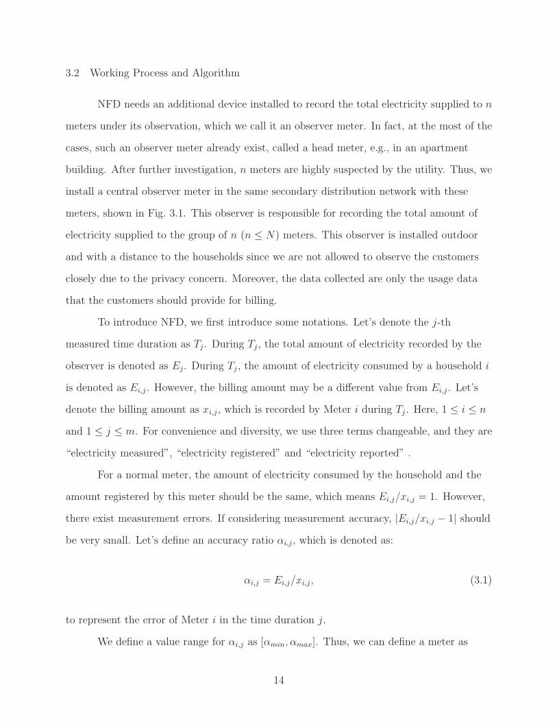
To introduce NFD, we first introduce some notations. Let’s denote the j-th
measured time duration as Tj. During Tj, the total amount of electricity recorded by the
observer is denoted as Ej. During Tj, the amount of electricity consumed by a household i
is denoted as Ei,j. However, the billing amount may be a different value from Ei,j. Let’s
denote the billing amount as xi,j, which is recorded by Meter i during Tj. Here, 1 ≤ i ≤ n
and 1 ≤ j ≤ m. For convenience and diversity, we use three terms changeable, and they are
“electricity measured”, “electricity registered” and “electricity reported” .
For a normal meter, the amount of electricity consumed by the household and the
amount registered by this meter should be the same, which means Ei,j/xi,j = 1. However,
there exist measurement errors. If considering measurement accuracy, |Ei,j/xi,j − 1| shouldbe very small. Let’s define an accuracy ratio αi,j, which is denoted as:
αi,j = Ei,j/xi,j, (3.1)
to represent the error of Meter i in the time duration j.
We define a value range for αi,j as [αmin, αmax]. Thus, we can define a meter as
14

Residential
Customer
Secondary
Distribution
Network
Observer
Meter
Electric vehicleCharging
spot
Meter 1
Meter 2
Meter 3
Meter 4
(a)
ObserverMeter
Meter 1 Meter 2 Meter i Meter n... ...(b)
Figure 3.1: Install an observer meter. a) An observer meter is installed along the pole side ina community and it records the supply to several suspected meters. These meters are eitherconnected to a household or a charging station for electric vehicles. b) This is the simplifiedmodel of the metering system.
15

normal when αi,j ∈ [αmin, αmax], where 1 ≤ i ≤ n and 1 ≤ j ≤ m. A typical value of αmin is
0.98 and a typical value of αmax is 1.02. Moreover, we can also believe that a meter is
tampered when αi,j > αmax. Each meter may have different accuracy, but the difference is
slight. We assume that all the meters have the same accuracy for simplicity.
(xi,j, i = 1, 2, · · · , n) are a series of the values of the billing electricity, and their
values are available. However, we do not know the values of (Ei,j, i = 1, 2, · · · , n). Thus, wecannot identify the tampered meters only by the comparison between xi,j and Ei,j. We
notice that there is a point at the coordinate for each value pair (xi,j, Ei,j), shown in
Fig. 3.2. For Meter i, there are a group of value pairs related to it, and we can use the
following function to represent these points:
yi = fi(x), where fi(xi,j) = Ei,j, j = 1, 2, · · · ,m. (3.2)
where that fi(x) stands for the behavior function of meter i and is what we need to figure
out.
Under the above assumptions, we have the following corollary, where the proof is
easy, and thus is omitted.
Corollary 3.1. For Meter i, it is a tampered meter, if and only if its curve, fi(x), is above
the line of f(x) = αmaxx.
Corollary 3.1 can be illustrated in Fig. 3.2. The curve of f5(x) is between the lines
of f1(x) = αmaxx and f6(x) = αminx, and it is regarded as a normal meter. When the
curves, such as the curves of f2(x), f3(x) and f4(x), are above the line of f1(x) = αmaxx,
their corresponding meters are regarded as tampered. Each point on the coordinate of
Fig. 3.2 is the value pair, (the measured electricity, the consumed electricity), of each
meter. The functions of these curves could be
• f(x) = ax+ b, where a and b are two constants, a > αmax, b ≥ 0;
• f(x) = xu, where u is a constant;
16

0
f1(x) = αmax x
..
..
.
.
..
.
..
.
....
.. .
......
.. ....... .. .. . .
...
f2(x) > αmax xf3(x) > αmax xf4(x) > αmax x
.
.
..... ...
. .. ... .. .
y
x
..
. .. ... .
. ..
αminx < f5(x) < αmax xf6(x) = αmin x
Point A = (xi, j , Ei, j)
Figure 3.2: Points on the coordinate, with the corresponding value pairs (the measuredelectricity, the consumed electricity). Curves of the normal meter and the possibly tamperedones. The black line is of the normal meter. Other curves above this line are differentpotential curves of the tampered meters according to Corollary 3.1.
17

• f(x) = ax, where a is a constant and a > 0, a �= 1;
• f(x) = a sin(bx+ c), where a, b, and c are three constants, and a > 0;
• f(x) = a arcsin(bx+ c), where a, b, and c are three constants, and a > 0;
• Other functions f(x) > αmaxx.
Algorithm 1 On-line NFD: NTL fraud detection
1: Initiation: choose n from N , choose initial m and mmax, set l = 02: for Each observer meter j do3: On Timer:4: each meter records observed value and registered value5: l ← l + 16: if l = mn then7: calculate [X] and [ET ]8: check linear independence of [X] and [ET ]9: if not linear independent then10: replace the last record with new measurement11: else12: kill timer13: calculate and normalize [A]14: obtain polynomial fi(x) of each meter i15: for each fi(x) do16: if fi(x) > αmaxx then17: identified as tampered18: if αminx ≤ fi(x) ≤ αmaxx then19: identified as normal20: else21: try a larger m22: break
Based on Lagrange polynomials, if we have m+ 1 samples, (xi,j, Ei,j), 0 ≤ j ≤ m, we
can find an approximation function to represent them, and this function can be written as
follows:
fi(x) =0∑
k=m
ak,ixk, (3.3)
where ak,i is the coefficients and fi(xi,j) = Ei,j.
If we know the values of the m+ 1 samples, we can obtain the coefficients (ak,i) by
direct calculation, and thus, get the function of Meter i using Eq. (3.3). But, till now we
18
only get to know the values of (xi,j, j = 1, 2, · · · ,m) and we do not know the values of
(Ei,j, j = 0, 1, · · · ,m).
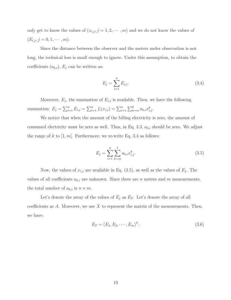
Since the distance between the observer and the meters under observation is not
long, the technical loss is small enough to ignore. Under this assumption, to obtain the
coefficients (ak,i), Ej can be written as:
Ej =n∑
i=1
Ei,j. (3.4)
Moreover, Ej, the summation of Ei,j is available. Then, we have the following
summation: Ej =∑n
i=1 Ei,j =∑n
i=1 fi(xi,j) =∑n
i=1
∑0k=m ak,ix
ki,j.
We notice that when the amount of the billing electricity is zero, the amount of
consumed electricity must be zero as well. Thus, in Eq. 3.3, a0,i should be zero. We adjust
the range of k to [1,m]. Furthermore, we re-write Eq. 3.4 as follows:
Ej =n∑
i=1
1∑k=m
ak,ixki,j. (3.5)
Now, the values of xi,j are available in Eq. (3.5), as well as the values of Ej. The
values of all coefficients ak,i are unknown. Since there are n meters and m measurements,
the total number of ak,i is n×m.
Let’s denote the array of the values of Ej as ET . Let’s denote the array of all
coefficients as A. Moreover, we use X to represent the matrix of the measurements. Then,
we have:
ET = (E1, E2, · · · , Em)T , (3.6)
19

A = (am,1, . . . , ak,1,, . . . , a1,1, a0,1, . . . ,
am,i, . . . , ak,i, . . . , a1,i, a0,i, . . . ,
am,n, . . . , ak,n, . . . , a1,n, a0,n) ,
(3.7)
X =
⎛⎜⎜⎜⎜⎜⎜⎜⎜⎜⎜⎜⎜⎜⎜⎝
xm1,1 . . . xk
1,1 . . . xn,1 1
xm1,2 . . . xk
1,2 . . . xn,2 1
......
......
......
xm1,j . . . xk
1,j . . . xn,j 1
......
......
......
xm1,nm . . . xk
1,nm . . . xn,nm 1
⎞⎟⎟⎟⎟⎟⎟⎟⎟⎟⎟⎟⎟⎟⎟⎠
, (3.8)
ET = X × A, (3.9)
A = X−1 × ET . (3.10)
The values of ET and X are available from the data of each measurement. Moreover,
we can obtain the values of X−1 by matrix inverse of X. Now, from Eq. (3.10), we get all
of the coefficients. One constraint of the n×m equations is that they should be linearly
independent. We can get all the polynomials by putting the coefficients into Eq. (3.3). For
each meter, there exists a polynomial to represent it. By analyzing the relationship
between a polynomial and f(x) = αmaxx, we can identify the tampered meters. If the curve
of a polynomial is above the line of f(x) = αmaxx at the coordinate, the related meter is
identified as tampered. If the curve of a polynomial is between the lines of f(x) = αmaxx
and f(x) = αminx, the related meter is identified as normal. If there is any curve of a
polynomial is under the line of f(x) = αminx, the detection process should report an error.
We aim to detect meters which are tampered on purpose to gain illegal benefits.
20

Thus, for each meter, its billing electricity is less than or equals to the amount of electricity
consumed. Colluding attacks occur when adversaries compromise a meter so that the
customer has to pay more than (s)he consumed. This problem is not what we want to solve
here, but it is our current research.
The proposed NFD algorithm can be used both on-line and off-line. For the off-line
detection, we need to identify NTL frauds out of a certain given dataset. Since the number
(n) of meters and the times of measurements are already known in the dataset, what we
need is to choose an appropriate order m, where m ≤ the times of measurements. For
the on-line detection, we need to gather data from each measurement and identify frauds
real time. The on-line detection algorithm can be seen in Alg. 1. It will choose an initial
order m and then keep gathering data until it gets enough data to build an independent
matrix. If the initial m is not satisfying, it will try a higher m and repeat the whole
process until it reaches either of the following two conditions:
1. Condition 1: every meter is identified as either tampered or normal;
2. Condition 2: m ≥ mmax and mmax is the maximum value of the desired order m.
The main steps of the detection process include preparation, calculation,
normalization, and comparison. In the first step, parameters are chosen to initialize the
process. In the second step, coefficients are obtained according to Alg. 1. In the third step,
the results are normalized. In the final step, we compare the polynomials with
f(x) = αmaxx to identify tampered meters.
We discuss parameter selection in details in Section 3.4.
3.3 Experiments
We conducted various experiments to test NFD, and some of the experiments are
introduced in this section. We use kWh as the unit for electricity values listed in the
tables. The data used in our experiments are simulated. According to a report [2], the
21

average household electricity usage around the world varies from 570 kWh to 11879 kWh in
2010. The experimental data are randomly generated within this range. We manually
altered some meters’ usage data letting the billing amount less than the original
(consumed) amount.
3.3.1 Experiment 1: No Tampered Meters
In this experiment, the dataset contains the data of 10 meter and an observer. We
list the data of 20 measurements, including the amount of the billing electricity and the
amount of the recorded value of the observer, shown in Table 3.1.
Table 3.1: The unit of the billed electricity (kWh) of 10 meters and an observer meter inNFD - Exp. 1
Meter 1 2 3 4 5 6 7 8 9 10 Observer
4560 3300 6780 1900 2870 3200 4510 2800 4320 5100 39340
5120 2560 4560 2440 1900 4500 5700 2120 5700 6700 41300
3230 3500 6780 3900 1670 5100 4340 2000 5200 6400 42120
6780 2900 5990 1890 2560 6700 5800 5300 6880 6890 51690
6430 3000 5300 2120 4980 7450 6400 3050 4990 4800 48520
1670 4300 5440 2800 5880 4560 6340 3560 4670 5120 44340
2430 2700 6330 3000 2200 1400 5300 3650 4770 5700 37480
7890 2300 4600 1900 2560 5700 4670 3670 2120 1440 36850
8700 3400 6120 2650 2780 6120 6400 3100 5670 5870 50810
4400 1400 3670 2990 2330 1670 4600 3540 5600 4660 34860
5200 2800 4780 2110 5430 3120 5600 3000 5900 4670 42610
3560 2900 5340 2440 5280 4230 5670 2890 4900 4220 41430
2450 4500 5200 2660 3760 5230 5800 2400 2220 2780 37000
4560 3890 5780 2770 4670 5400 6200 2670 3450 3990 43280
3670 2700 6400 3120 4980 6400 6900 2670 3560 6450 46850
3560 4100 5990 3450 4330 4780 6770 1990 4110 5980 45060
2340 3330 6900 3200 3780 1560 5440 2500 4560 5840 39450
5320 3990 5550 3320 4550 9530 6780 5700 4880 6330 55950
3240 3980 5090 1990 2670 4500 7000 3890 4670 5300 42330
4670 2900 4200 2550 4670 8670 7100 3600 5450 8120 51930
In this experiment, we use the Lagrange polynomial with order 2. Since the dataset
only contains the data of 20 measurements, we cannot use an order higher than 2.
22

Moreover, the polynomial is as follows:
fi(x) = a2,ix2 + a1,ix. (3.11)
Based on Eq. (3.10), we can get the values of A. After calculation and
normalization, we get
A = (0, 1, 0, 1, 0, 1, 0, 1, 0, 1, 0, 1, 0, 1, 0, 1, 0, 1, 0, 1).
The obtained polynomials of all meters are shown in the second column of Table 3.2.
We compare the polynomials with f(x) = αmaxx and find that none of the meters are
tampered. In other words, there are all normal meters.
Table 3.2: The results of the experiments: the polynomials of all meters. There are 10 metersin Experiments 1 and 2, respectively, and 4 meters in Experiment 3.No. Experiment 1 Experiment 2 Experiment 3 Lowering order1 f1(x) = x f1(x) = x f1(x) = 0.1x2 + x f1(x) = −0.265x2 + 1.308x2 f2(x) = x f2(x) = x f2(x) = 0.5x2 + 0.3x f2(x) = 1.123x2 − 6.308x3 f3(x) = x f3(x) = x f3(x) = 0.1x2 + 0.9x f3(x) = 0.006x2 + 0.265x4 f4(x) = x f4(x) = x f4(x) = 0.3x2 + x f4(x) = 0.458x2 − 1.681x5 f5(x) = x f5(x) = x N/A f5(x) = −0.004x2 + 0.845x6 f6(x) = x f6(x) = x N/A f6(x) = −0.338x2 + 6.128x7 f7(x) = x f7(x) = 0.1x3 + 0.5x2 + x N/A f7(x) = 1.8x2 − 3.32x8 f8(x) = x f8(x) = x N/A f8(x) = −0.42x2 + 3.32x9 f9(x) = x f9(x) = x N/A f9(x) = −0.21x2 − 0.41x10 f10(x) = x f10(x) = x N/A f10(x) = 0.11x2 + 0.364x
3.3.2 Experiment 2: Single Adversary and Single Tampered Meter
In this experiment, the dataset contains the data of 10 meters and an observer.
Table 3.3 shows the values of the amount of the billing electricity and the amount of the
supplied electricity recorded by the observer in 30 measurements.
In this experiment, we employ the polynomial with an order of 3, which is as follows:
fi(x) = a3,ix3 + a2,ix
2 + a1,ix. (3.12)
23

Table 3.3: The unit of the billed electricity (kWh) of 10 meters and an observer meter inNFD - Exp. 2
Meter 1 2 3 4 5 6 7 8 9 10 Observer
2110 3300 4710 1500 3000 8230 4500 2800 4600 5300 59287.5
1950 2600 5330 2330 1530 8550 5600 4494 5100 5600 73951.6
1800 3500 6600 2560 1990 9000 4800 2000 5200 6100 66129.2
2220 2900 6780 1890 2560 9980 5120 5000 6780 6990 76749
2300 3000 4990 2120 4560 8770 6000 3050 4900 4670 83960
1570 3700 6100 2890 5660 8990 6340 3500 4880 5120 94331.8
2500 2700 6230 3000 2200 7990 5300 3600 4780 5330 72562.7
2300 3200 4780 1900 2560 8230 4990 3670 2100 5900 64505.2
2880 3400 5330 2440 2890 8450 4890 3090 5800 5810 68629.1
1930 3100 3550 2670 2330 8650 4600 3550 5700 4890 61283.6
2120 2500 4880 2110 5330 8100 4500 2990 5550 4550 61867.5
2300 2900 4940 2230 5280 7450 5670 2890 4900 4200 77062.9
2000 2900 5120 2660 3600 7810 5800 2700 2100 2600 736212
1750 4000 5440 1990 4670 9110 6200 2560 3600 3900 86272.8
1820 2700 5980 3120 4880 9300 6900 2670 3700 6230 103955.9
2740 2760 5770 3450 4330 8560 6770 1900 4100 6430 100755.3
2450 3330 4890 3330 3990 8440 5440 2500 4800 5810 75875.7
2530 3670 5220 3320 4550 9400 6450 3060 4900 6300 97034.9
2320 3980 5540 1970 2550 9910 6340 3560 4780 5900 92431.8
2780 2990 5900 2550 3890 8760 6100 3880 5600 5660 89413.1
2300 3450 6780 1770 3200 7770 5990 3660 1200 1900 77452.2
3450 4320 7120 1800 3560 7650 5870 3400 1340 1980 77944.7
5320 2450 8120 2890 4120 8010 5770 3080 2450 200 78266.5
4340 3090 7890 3120 4030 7990 5050 2090 2980 4500 70710
2630 4670 6120 3450 2120 7120 6120 4090 2100 5230 85299.3
3120 5120 6660 3200 2670 6890 4890 3900 3210 6120 69429.1
3090 3100 6450 4300 3400 6770 4990 3890 4500 5900 71265.2
1980 3980 5700 3780 3080 6080 5340 3100 4090 4980 71595.1
2890 4560 7230 3880 3030 6130 5220 2030 1900 4870 69587.9
2770 3900 7450 3200 3980 7450 5090 2450 2890 800 66121.3
24

Using Eq. (3.10), the values of A can be obtained. The results after normalization
are as follows:
A = (0, 0, 1, 0, 0, 1, 0, 0, 1, 0, 0, 1, 0, 0, 1,
0, 0, 1, 0.1, 0.5, 1, 0, 0, 1, 0, 0, 1, 0, 0, 1).
The polynomials of all the 10 meters in this experiments are shown in the third
column of Table 3.2. The curves of meters are shown in Fig. 3.3. After comparing between
these polynomials and f(x) = αmaxx, we notice that the curve of the 7th meter is above the
line of f(x) = αmaxx. Thus, the 7th meter is a tampered meter.
3.3.3 Experiment 3: Multiple Adversaries and Multiple Tampered Meters
In this experiment, the dataset contains the data of 4 meters and an observer. The
amount of the billing electricity and the amount of the supplied electricity in 8
measurements are listed in Table 3.4. We employ the polynomial with an order of 2, which
is the same as in Exp. 1.
Table 3.4: The unit of the billed electricity (kWh) of 4 meters and an observer meter inNFD - Exp. 3
Meter 1 Meter 2 Meter 3 Meter 4 Observer Meter
2100 4000 3000 6700 35508
1800 5000 4000 10300 63451
2500 3600 8000 4500 34860
1900 5300 6000 5600 41904
2200 6300 7000 8900 68282
2600 4000 4500 9400 54459
3000 5000 3400 8700 53523
1700 3000 3700 8600 42876
Now we can obtain A, according to Eq. (3.10). After calculation and normalization,
we get
A = (0.1, 1, 0.5, 0.3, 0.1, 0.9, 0.3, 1).
The obtained polynomials of all the meters in this experiment can be seen in the
fourth column of Table 3.2. After comparing these polynomials with f(x) = αmaxx, we find
25

4.5 5 5.5 6 6.5 70
10
20
30
40
50
60
70
The value of the measured electricity − x
Th
e va
lue
of
the
con
sum
ed e
lect
rici
ty −
f(x
)
NormalTampered
(a)
0 2 4 6 8 100
5
10
15
20
The value of the measured electricity − x
The
valu
e of
the
cons
umed
ele
ctric
ity −
f(x)
NormalTampered
(b)
Figure 3.3: The curves of all the polynomials in Experiment 2. The range of x shown in a)isobtained from the related dataset. The range of x in b)is extended to [0,10].
26

0 2 4 6 8 100
5
10
15
20
25
30
35
40
The al e of he mea red elec rici
The
ale
ofhe
con
med
elecr
icif Normal
Me er1Me er2Me er3Me er4
(a)
0 2 4 6 8 100
10
20
30
40
50
60
The al e of he mea red elec rici
The
ale
ofhe
con
med
elec
rici
f NormalMe er1Me er2Me er3Me er4
(b)
Figure 3.4: The curves of all the polynomials in Experiment 3. The range of x shown in a)isobtained from the related dataset. The range of x in b)is extended to [0,10].
27

that all the meters are tampered meters. The curves of these meters, with a comparison to
the normal meter, are shown in Fig. 3.4.
3.4 Parameter Selection and Discussion
The selection of the order m is decided by accuracy requirement. If a higher
accuracy is required, a bigger m is needed, at the most of the time. Also, more
measurement data are needed to obtain a polynomial with a higher order of m. However, a
bigger m not always results in a higher accuracy.
In this section, some discussions will be carried out to guide applicable usage of this
scheme. Theoretical analysis and related proofs will be carried out, together with some
case studies. Its main purpose is to answer the following questions:
• How to choose the order m?
• For a given order m, what should the error be?
• To lower the error, should we choose a higher m?
• For a given order m, how many measurement data do we need?
• How many meters should be in the same group (how to choose n)?
• How much detection time is needed to identify a fraud?
• How many observer meters are needed in a community?
3.4.1 Error and Selection of Order m
In this subsection, we’ll discuss the relationship between the order m and the
corresponding error. Related theoretical analysis and case study will help to choose a
better value of the order m.
28

Now, we’ll use the same dataset in Experiment 2 to illustrate the error. In
Experiment 2, we use an order 3 polynomial to fit the dataset. Here, we try to use an order
2 polynomial to fit the dataset. The result is shown in Table 3.2.
From Table 3.2, the last column, maybe it is hard to identify the tampered one. But
it is easy to differentiate the tampered meter from those normal meters in Fig. 3.5. The
black line is the normal meter with the polynomial of f(x) = αmaxx. The lines or curves
above this black one are suspected to be tampered. We can see that only the curves of
Meter 6 and Meter 7 are above it. Moreover, for Meter 6, its slope rate is almost the same
as the normal meter. Meter 7’s curve is far from the normal one with a sharper slope.
Meter 7 is tampered, as the result of Experiment 2. But for Meter 6, it is a false alarm.
The reason is that to get the order 2 polynomial, we only need 20 out of the total 30
measurements dataset in Experiment 2. The occurrence of error is caused by lower
accuracy. Reversely, to identify the tampered meters accurately, more data or
measurements are needed.
4.5 5 5.5 6 6.5 720
10
0
10
20
30
40
50
60
70
80
90
The value of the measured electricity − x
The
valu
e of
the
cons
umed
ele
ctric
ity −
f(x)
Me erlMe er2Me er3Me er4Me er5Me er6Me er7Me er8Me er9Me er10Normal
Figure 3.5: The curves of the polynomials in the experiment of lowering order. A false alarmoccurs when using an order-2 polynomial instead of an order-3 polynomial.
29

4.5 5 5.5 6 6.5 720
30
40
50
60
70
The al e of he mea red elec rici
The
ale
ofhe
con
med
elec
rici
f
f =1.8 2 3.32f =0.1 3 0.5 2
(a)
0 2 4 6 8 1050
0
50
100
150
200
The al e of he mea red elec rici
The
ale
ofhe
con
med
elec
rici
f
f =1.8 2 3.32f =0.1 3 0.5 2
(b)
Figure 3.6: Error comparison between the order 2 and order 3 polynomials of the same meter- Meter 7, obtained from the same dataset in the experiment. The range of x shown in a)isobtained from the related dataset. The range of x in b)is extended to [0,10].
30

The comparison of the order 2 and order 3 curves of the same meter - Meter 7, is
shown in Figs. 3.6(a) and (b). The range of x in Fig. 3.6(a) is the same as in the
experimental dataset. Fig. 3.6(b) shows the curves where x is in [0, 10].
The error between the approximation polynomial and its original function,
according to Lagrange remainder theorem [54], can be given as:
Rn(x) =fn+1(ξ)
(n+ 1)!(x− x0)
n+1, ξ ∈ [x0, x]. (3.13)
However, we cannot get to know the original form of the function only from two of its
approximation polynomials. Here, we propose another method, to estimate the error of
lowering order. Let’s define:
e is the error of lowering the order;
xi is the value of the measured electricity in each Meter i;
f1(xi) is the corresponding value of xi in the lower-order polynomial f1(x);
f2(xi) is the corresponding value of xi in the higher-order polynomial f2(x);
n is the number of sample points obtained from each of the polynomials.
Definition 3.1. Assume that a meter has two polynomials, f1(x) and f2(x), which are
obtained from the same dataset of measurements, where f2(x) is the higher-order
polynomial and f1(x) is the lower-order polynomial. Their relative error is given by:
e =
√√√√√xn∑
xi=x1
(f1(xi)−f2(xi)f1(xi)
)2n
. (3.14)
Conjecture 3.1. The error - e given in Definition 3.1 can describe the relative error of
two polynomials with different orders obtained from the same dataset. Its accuracy is in the
same order of magnitude of Lagrange remainder as given in Eq. (3.13).
Now consider the function f(x) = 2 sin(x). Its Taylor approximation, when x0 = 0,
is as follows:
31
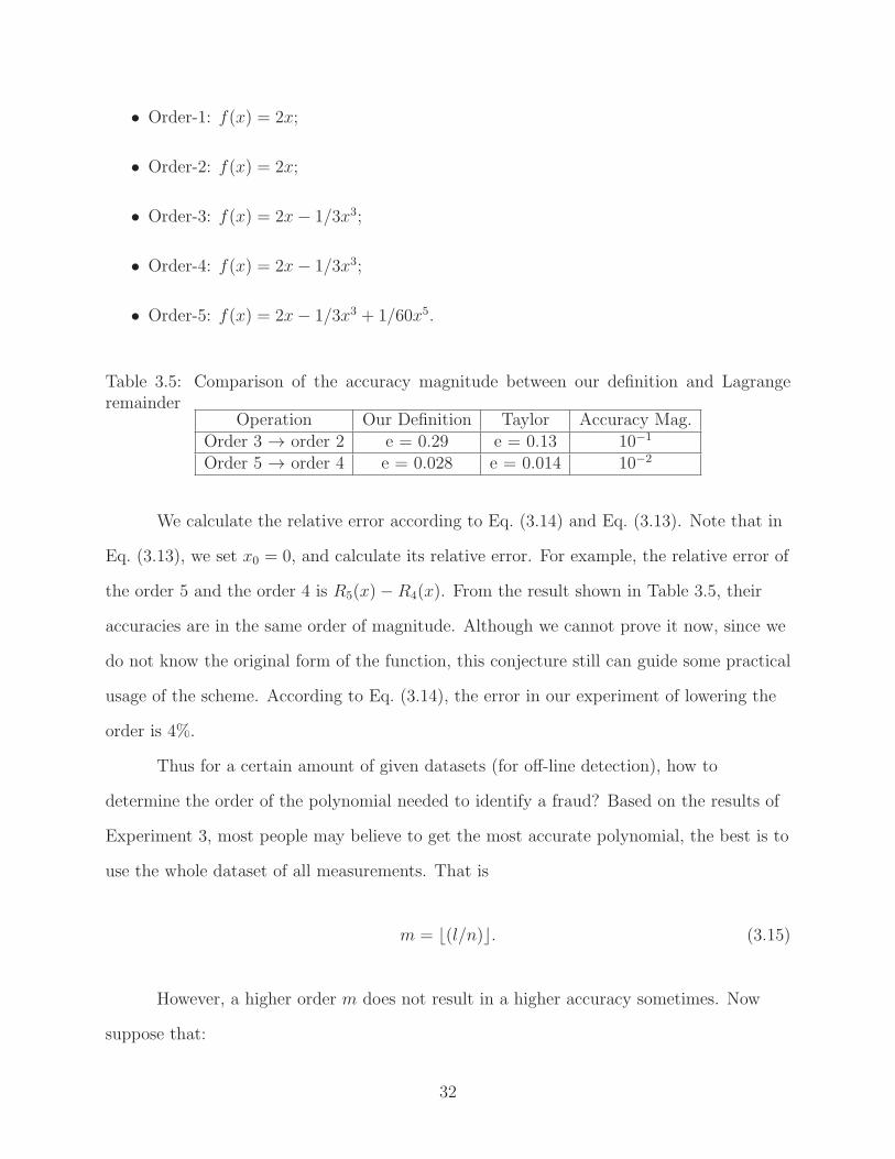
• Order-1: f(x) = 2x;
• Order-2: f(x) = 2x;
• Order-3: f(x) = 2x− 1/3x3;
• Order-4: f(x) = 2x− 1/3x3;
• Order-5: f(x) = 2x− 1/3x3 + 1/60x5.
Table 3.5: Comparison of the accuracy magnitude between our definition and Lagrangeremainder
Operation Our Definition Taylor Accuracy Mag.Order 3 → order 2 e = 0.29 e = 0.13 10−1
Order 5 → order 4 e = 0.028 e = 0.014 10−2
We calculate the relative error according to Eq. (3.14) and Eq. (3.13). Note that in
Eq. (3.13), we set x0 = 0, and calculate its relative error. For example, the relative error of
the order 5 and the order 4 is R5(x)−R4(x). From the result shown in Table 3.5, their
accuracies are in the same order of magnitude. Although we cannot prove it now, since we
do not know the original form of the function, this conjecture still can guide some practical
usage of the scheme. According to Eq. (3.14), the error in our experiment of lowering the
order is 4%.
Thus for a certain amount of given datasets (for off-line detection), how to
determine the order of the polynomial needed to identify a fraud? Based on the results of
Experiment 3, most people may believe to get the most accurate polynomial, the best is to
use the whole dataset of all measurements. That is
m = �(l/n). (3.15)
However, a higher order m does not result in a higher accuracy sometimes. Now
suppose that:
32

• The number of meters is n;
• The total time of measurements is l, only refer to the measurements with complete
data;
• The needed order of the polynomial is m.
Theorem 3.1. Obtaining more measurements or using a larger historical dataset to obtain
a polynomial with a higher order does not always improve the accuracy of the polynomial.
Proof. see Appendix A.
Theorem 3.1 tells us that a higher order m does not always increase the detection
accuracy. In Theorem 3.1, we present two lemmas. Lemma A.1 tells us when a higher
order m can increase the detection accuracy, and Lemma A.2 tells us when a higher order
m cannot increase the detection accuracy.
Under some circumstances, if the dataset is too large, we need to choose a subset of
the data measured, and to get a relatively lower but good m. The criterion that we
propose is to constrain the error - e, as in Eq. (3.14), within the accuracy class. That is
e < |α− 1| . (3.16)
Under some circumstances, if the dataset is too small for more accurate analysis, or
we need a shorter detection time, we can ignore some coefficients, to get a better result
with limited data.
Lemma 3.1. With limited data gathered, ignoring a0 can improve accuracy and save
detection time. That is: when l ≤ 3n, where l is the number of measurements with complete
data gathered,
fi(x) = am,ixm + am−1,ix
m−1 + · · ·+ ak,ixk + · · ·+ a1,ix. (3.17)
33

Proof. Compare it to Eq. (3.3). For n meters, Eq. (3.17) needs n fewer times of
measurements to get the result so that it will save detection time. Moreover, based on the
same dataset, with Eq. (3.17) we can get one order higher than with Eq. (3.3). According
to Lemma A.1 (see Appendix A), with Eq. (3.17), we can get a higher accuracy. Note that
the situation mentioned in Lemma A.2 (see Appendix A), only occurs in high order
approximation, rather than ≤ 5 order.
For most on-line cases, m can be chosen as 2 initially, and according to Alg. 1, m
can be adjusted to a higher order towards mmax. In most off-line cases, mmax can be
chosen as 3 to 5, according to different sizes of datasets. Typically, an order of mmax = 5 is
enough for most practical applications.
3.4.2 Detection Time and Selection of User Number n
In this subsection, we will discuss fraud detection time, how to select n out of the
total N users or meters in a community, and the number of observer meters needed.
The detection time t is decided by the desired order m, the number of meters under
observation n, and the time interval of measurement T0. It’s given as
t = mnT0. (3.18)
In Smart Grid, if we expect to detect NTL frauds within 6 hours, where the
metering interval is set to be 15 minutes typically [36], one observer meter can observe 8
meters at most, and the desired m is 3. In a community with N meters, at least, N/8�observer meters should be installed. Inversely, if consider from the angle of saving budget,
installing one observer meter for each community is considerable. In the traditional power
grid, the time interval for measurement may be much longer than in Smart Grid, because
of the difficulty of gathering data. If we can get data once per day, we need at least 24 days
to achieve the same effect as in Smart Gird. Now consider saving the detection time and
34

the budget at the same time. We can set different weights or priorities for the detection
time and the budget.
Let’s denote w1 as the weight of the detection time and w2 as the weight of the
number of the observer meters, respectively. Here, fewer observer meters means less budget
needed. We define o as the number of the observer meters installed in a community.
Theorem 3.2. To balance the budget and the detection time in NFD, the number of the
observer meters o must satisfy the following equation:
o =
√w1mNT0
w2
, (3.19)
and the number of meters n monitored by one observer cannot exceed:
n ≤√
Nw2
w1mT0
. (3.20)
Proof. Let’s define y as:
y = w1t+ w2o. (3.21)
To balance the budget and the detection time in NFD, y should be minimized. We notice
that
n = N/o, (3.22)
and put n into Eq. (3.18), we get
t = mNT0/o. (3.23)
Now, put t into Eq. (3.21), we get
y = w1tmNT0/o+ w2o
≥ 2√w1mNT0w2.
(3.24)
35

When o =√
w1mNT0
w2, y is the minimal, and the value is 2
√w1mNT0w2. Moreover, the
related detection time t is mNT0w2
w1.
Correspondingly, according to Eq. (3.22), the number of meters monitored by one
observer cannot exceed√
Nw2
w1mT0.
3.5 Conclusion
In this chapter, a novel detector NFD is proposed to detect NTL frauds in Smart
Grid. NFD is based on Lagrange polynomials to generate a polynomial for each meter
using a small dataset. By comparing the polynomials between the normal meters and the
abnormal meters, we can identify tampered meters. Various experiments have been
conducted to show the effectiveness of NFD. A detailed discussion about parameter
selection, together with mathematical proofs and case study, have guided its way to
real-world practical applications. As a future work, we will further study the conjecture in
this chapter. Moreover, for the on-line detection algorithm, we will set up a series of
experiments to test its false alarm rate and efficiency in real-world applications.
Note that NFD does not like a traditional security solution such as intrusion
detection system (IDS) where how to choose a good detection threshold is an important
aspect. Instead, NFD uses a non-traditional approach to tackle a security problem. Our
focus is not how to choose a better detection threshold, but presenting our method and the
foundation of the method in general. How to choose a better threshold will be our future
research.
36

CHAPTER 4
FNFD: FAST NTL FRAUD DETECTION AND VERIFICATION
4.1 Introduction
To improve the detection speed, a detector named FNFD (fast NTL) [28, 29] is
proposed in this chapter. FNFD can detect NTL frauds with a small amount of data. The
detection speed of FNFD is much faster than the existing detectors. FNFD can detect
multiple tamered meters as well as a single tampered meter in a group. Moreover, FNFD
has a new function, fraud verification. Fraud verification is to verify a pre-existed NTL
fraud. Existing detectors have to redo the whole detection process to verify a fraud, but
FNFD only needs one more step. Instead of analyzing user behavior, FNFD analyzes
adversary behavior and builds adversary models based on the analysis. The models are
built on linear functions, e.g. Recursive Least Square (RLS) [34]. Thus, the detection speed
of FNFD is faster than the detector whose model is built on polynomials [26].
4.2 Working Process and Algorithm
We install a central observer meter along the pole side in the community, where a
group of n (n ≤ N) smart meters are connected, shown in Fig. 3.1. The purpose of
introducing this observer is to record the total amount of electricity supplied to the n
meters. We assume that the measurement of the observer is accurate and it is well-secured.
We attach a tamper-resistant device to the observer and monitor it with intensive
surveillance. Due to budget and privacy consideration, we cannot equip each meter with a
tamper-resistant device and cannot observe each meter closely. The smart meters report
power consumption periodically.
37

Typically, meters are read every 15 minutes in Smart Grid [36]. Therefore, a typical
value of Tj is 15 minutes, but Tj could be smaller or larger theoretically. The value of Eij
must be greater than the value of xij if it is an NTL fraud. If it is not an NTL fraud, the
value of Eij should be almost the same as xij. We use a coefficient ai to represent a meter
i, and ai may have different values in different Tj which is defined as:
aij = Eij/xij. (4.1)
Thus, a meter is normal when aij = 1, and it is tampered when aij > 1. Let’s use
the notation η as the measurement accuracy. A meter is normal when 1− η ≤ aij ≤ 1 + η,
and it is tampered when aij > 1 + η. Typically, the value of η is set to 2%. We assume that
meters have the same measurement accuracy based on the observation that the difference
is slight although measurement accuracy varies. To make it concise, we define αmin and
αmax as:
αmin = 1− η, (4.2)
and
αmax = 1 + η, (4.3)
respectively. Thus, when aij > αmax, the meter is tampered. When
αmin ≤ aij ≤ αmax, the meter is normal.
aij, the coefficient of a meter is obtained from the data of one measurement.
However, the value aij varies with Tj for each meter. We should obtain a stable coefficient
ai to represent a meter. If we think of xij as x and Eij as y, we can get a point B at the
coordinate shown in Fig. 4.1. Correspondingly, a group of (xij, Eij) value pairs have a
group of scattered points at the coordinate show in Fig 4.1. We cannot get a function with
these points on it. However, finding a line which is the closest to these points is feasible.
38

We take the coefficient of the line as the coefficient of the meter. The lines are denoted as:
fi(x) = aix. (4.4)
It is easy to prove that a tampered meter has a line above the line of f1(x) = αmaxx.
0
f1(x) = αmax x
..
. ..
.
..
.
..
...
..
.. .
.....
.
.. .. .. ..... ... .
...
f2(x) > αmax xf3(x) > αmax xf4(x) > αmax x.
... .
.. .... .. .
.. .. .
y
x
..
. .. ... .
. ..
αminx < f5(x) < αmax xf6(x) = αmin x
Point B (xi j , Ei j)
Figure 4.1: Each point at the coordinate represents a pair of values, that is (the amount ofthe measured electricity, the amount of the consumed electricity) of a meter. A line is usedto fit each group of points. The black line is the typical line of a normal meter. A tamperedmeter has a line above the black line and lines of tampered meters are different.
We only have limited measurement data. How can we generate these lines? We
notice that
Ej =n∑
i=1
Eij, (4.5)
and Ej is available since it is recorded by the observer. We re-write it in the following:
Ej =n∑
i=1
aixij. (4.6)
Xj is the vector of the values of the j-th measurement. A is the vector of all
39

coefficients. We have:
A = (a1, a2, . . . , an). (4.7)
Xj = (x1j, x2j, . . . , xnj). (4.8)
We use rij to denote the distance from a point to the closest line of Meter i in Tj,
which is defined as:
rij = Eij − fi(xij) (4.9)
The closest line is defined as the summation of the distances rij is the minimal, and
the summation is denoted as:
S =m∑j=1
r2ij. (4.10)
Now, the problem becomes a Least Square (LS) problem
S → minimum. (4.11)
If the data of all the measurements and the values of Eij are available, this problem
can be solved via matrix inversion. However, the measurement data are not available and
they come in one by one in real time. We do not know Eij, too.
We suppose that an estimation of A is available after j − 1 times of measurements,
which is Aj−1. The data of a new measurement Xj and Ej come in, and we need to update
Aj−1 with the new data. Based on the idea of RLS, to get a new estimation Aj, we have:
Aj = Aj−1 +Wj(Ej −XjAj−1), (4.12)
where
Wj = Pj−1XTj (λ+XjPj−1X
Tj )
−1, (4.13)
40

Pj = (I −WjXj)Pj−1/λ, (4.14)
P−1j = λP−1
j−1 +XTj Xj. (4.15)
Here, I is the identity matrix. W is an array of weight. The value of P shows the degree of
precision of the measurement. P is initialized with P0 = kI, where k is a constant with a
high value. λ is a forgetting factor which has a value between 0 and 1 (0 < λ ≤ 1). The
main function of λ is to “forget” the old measurements. The level of affection of the old
data is decided by the concrete value of λ. The affection decreases with the increase of λ.
To decrease the affection of the old data, a smaller value of λ is preferred. Introducing λ to
FNFD makes it more flexible in real-world applications, where the situation of each case
varies.
Algorithm 2 FNFD: fast NTL fraud detection and verification
1: Initiation: set initial values of n, αmin, αmax, Aj−1, λ and k. Set Pj−1 = kI. j startsfrom 1 in fraud detection, and starts from any number in fraud verification.
2: repeat3: record the value of observer meter Ej in each time period j,
record the value array of all other meters Xj in each time period j,Wj ← Pj−1X
Tj (λ+XjPj−1X
Tj )
−1,Aj ← Aj−1 +Wj(Ej −XjAj−1),Pj ← (I −WjXj)Pj−1/λ
4: until Aj doesn’t change5: for each ai in Aj do6: if ai > αmax then7: identified as tampered8: if αmin ≤ ai ≤ αmax then9: identified as normal10: else11: report error
FNFD fraud detection and verification algorithm is shown in Alg. 2. The processes
of detection and verification look similar to each other. In fact, the unified process is one of
the attracting features of FNFD which makes things simple. In fraud detection, j has to
start from 1 since there are no historical data or estimations available. Moreover, we need
to set values for A0 and P0 to get started. In fraud verification, j could start from any
41

number, since Aj−1 is already known. The verification process may take only one step and
we can get a new result.
4.3 Experiments
Various experiments have been carried out to test the performance of FNFD. To
show the effectiveness and performance, we conducted the same experiments on FNFD,
NFD, DCI, and BCGI, introduced in the related work section earlier. We choose three
typical experiments and presented in this section. The parameters are chosen as follows:
the value of λ is set to 0.01, k is set to 100, and the value of ai is 2. The value of η is set to
2%, and correspondingly αmax has a value of 1.02, and αmin is 0.98. A normal meter has a
line falling in the range between 0.98 and 1.02. A tampered meter has a line falling in the
range above 1.02. FNFD reports an error when any line of a meter is below 0.98. All the
data in the experiments are simulated. Normal consumption range, family/business size,
season, weather and other variations are considered when we randomly generate usage
data. Then abnormality is added into the normal data.
4.3.1 Detect a Single Tampered Meter
This experiment is to test FNFD on detecting a single tampered meter when the
other meters are normal. Table 4.1 shows the data set containing the data of 20
measurements.
The converging process of the coefficients of the 10 meters in Exp. 1 is shown in
Fig. 4.2. The coefficients change step by step with the data input of each measurement.
After the 10th step, the coefficients of all meters converge to fixed values. The coefficient of
Meter 4 converges to 1.33. The other coefficients converge to 1. The converging process
shows that Meter 4 is tampered and other meters are normal. The same experiment is
conducted to test NFD, and NFD can identify Meter 4 as tampered at the 20th step. The
input dataset for NFD contains 20 measurements. It shows that FNFD can double the
detection speed of NFD and needs half of the data.
42

Table 4.1: The unit of the billed electricity usage (kWh) of 10 meters and 1 observer inFNFD - Exp. 1
Meter 1 2 3 4 5 6 7 8 9 10 Observer
2750 3450 5520 2290 3310 9040 4630 3650 5020 5850 46270
2810 3330 6310 3230 1960 9020 5640 2750 5140 6130 47390
2570 4000 6750 3140 2430 9190 5490 2000 5350 6170 48130
2510 3470 6810 2320 3400 10280 6070 5690 7430 7280 56030
3180 3460 5780 2970 5110 9290 6570 3210 5530 5300 51380
2050 4600 7100 3110 6420 9800 6940 3790 5580 6000 56420
3190 3040 7180 3740 2250 8850 6120 3780 5350 5980 50710
2460 3950 5380 1960 3430 9170 5580 4260 2860 6860 46560
3610 4050 5410 2740 3870 9180 5480 3410 6250 6670 51570
2050 3500 4330 3400 3040 9550 5200 4460 6040 5100 47790
2740 3180 5160 2960 5910 8560 5450 3800 5990 5410 50140
2580 30510 5390 2680 6190 7500 6210 3370 5750 4350 48410
2060 3040 5700 3660 4090 7860 6350 2870 3020 3470 43330
2680 4690 5920 2030 5540 9950 7130 3230 4470 4420 50730
2520 3330 6490 3720 5250 9380 7820 3400 4620 6300 54060
3510 3200 6340 4410 4510 9190 7660 2710 4720 6700 54410
3100 3500 5330 4000 4620 8730 5960 2900 5330 6580 51370
2810 4290 5930 4010 5290 9740 6820 3900 5660 6500 56270
2330 4850 6410 2830 3080 10570 6660 4150 5070 6380 53260
2980 3440 6430 2710 4200 9660 6530 4820 6090 6390 54140
The same dataset and experimental settings are used to test BCGI and DCI.
However, BCGI cannot work with only one observer (inspector). To observe 10 meters,
BCGI needs at least 4 observers which is a huge cost. DCI can identify Meter 4 as the
tampered meter at the 7th or 8th step, which is decided by the binary tree structure. In
hundreds of experiments that we conducted, this is the best case of DCI. DCI is good at
detecting a single tampered meter under the condition that we know there is exactly one
tampered meter in a group. However, we cannot get to know how many meters are
tampered in advance.
4.3.2 Detect Multiple Tampered Meters
This experiment is to show the effectiveness of detecting multiple tampered meters
in a group. Table 4.2 shows the data set containing the data of 20 measurements.
The converging process of the coefficients of the 10 meters in Exp. 2 is shown in
43

Figure 4.2: The converging process of the coefficients of the 10 meters in Exp. 1. Thecoefficient of Meter 4 converges to 1.33, while the coefficients of other meters converge to 1.It shows that Meter 4 is the tampered meter.
Figure 4.3: The converging process of the coefficients of the 10 meters in Exp. 2. Thecoefficients of Meters 1, 2, 4, 8 and 10 converge to 2, 1.5, 3.2, 1.2 and 1.6, respectively, andthe coefficients other meters converge to 1. It shows that Meters 1,2,4,8 and 10 are tamperedand other meters are normal.
44

Table 4.2: The unit of the billed electricity usage (kWh) of 10 meters and 1 observer inFNFD - Exp. 2
Meter 1 2 3 4 5 6 7 8 9 10 Observer
2190 3620 5520 1950 3160 8620 5390 2990 5530 5590 56802
2220 2980 6310 2700 1890 9300 6030 2650 5330 5600 58550
1890 3510 7110 2720 2330 9060 5120 2570 5780 6790 61097
2330 3640 7060 2060 3270 10690 6050 5070 7470 7060 68632
3090 3160 5610 2750 4650 9130 6300 3800 5280 5630 64258
2480 3860 6110 3440 5820 9290 6950 3920 5830 5290 68926
3360 3550 6660 3610 2450 8000 5930 4390 5610 5560 66411
3130 4010 4810 2510 3380 8270 5830 3790 2190 6400 59575
3080 4360 5460 2660 3480 9120 5670 3540 6330 6520 65952
2440 3980 4230 3490 2390 9440 4880 4140 6610 4980 62504
2180 2510 5820 2160 5540 8230 4650 3450 5730 5140 57371
2850 3390 5120 3040 5450 7650 6430 3680 5860 4310 62335
2780 3280 5540 3220 3970 8530 6260 2970 3050 2790 56162
2480 4610 6380 2470 5430 9400 6570 3330 3630 4640 62609
2280 3500 6710 3920 5420 9990 7310 3110 3710 6470 69578
3400 3170 5810 4160 4680 9110 7270 2740 4360 7070 70697
2560 3810 5060 3830 4520 9120 5610 3330 5290 5820 65999
910 3900 6110 3950 5300 10090 7190 3270 4910 6610 72410
3270 4670 5720 2540 3230 10380 7240 3680 5420 6300 68159
3330 3730 6020 2690 4390 9310 6730 4640 6380 6030 68909
Fig. 4.3. The coefficients change in each step with the data input of each measurement.
After the 10th step, the coefficients of the meters converge to fixed but different values.
The coefficients of of Meters 1,2,4,8 and 10 converge to 2, 1.5, 3.2, 1.2 and 1.6, respectively.
The other coefficients converge to 1. The converging process shows that Meters 1,2,4,8 and
10 are tampered and other meters are normal. The same experiment is conducted to test
NFD, and NFD can identify Meters 1,2,4,8 and 10 as tampered at the 20th step. The input
dataset for NFD contains 20 measurements. It shows that FNFD can double the detection
speed of NFD and needs half of the data.
The same dataset and experimental settings are used to test BCGI and DCI. BCGI
cannot normally function and fails to get a result. DCI can identify the tampered meters
at the 16th to 19th step, which is up to how the binary tree is constructed. In hundreds of
experiments that we conducted, this is the average case of DCI. DCI is not good at
45

detecting multiple tampered meters in one group.
4.3.3 Detect All Tampered Meters
This experiment is to test the effectiveness of detecting meters in a group that are
all tampered. The data set containing the data of 20 measurements is shown in Table 4.3
Table 4.3: The unit of the billed electricity usage (kWh) of 10 meters and 1 observer inFNFD - Exp. 3
Meter 1 2 3 4 5 6 7 8 9 10 Observer
5560 4300 7780 2900 3870 4200 5510 3800 5320 6100 95491.8
6120 3560 5560 3440 2900 5500 6700 3120 6700 7700 98946.8
4230 4500 7780 4900 2670 6100 5340 3000 6200 7400 101094.4
7780 3900 6990 2890 3560 7700 6800 6300 7880 7890 117942.1
7430 4000 6300 3120 5980 8450 7400 4050 5990 5800 112707.4
2670 5300 6440 3800 6880 5560 7340 4560 5670 6120 109290.2
3430 3700 7330 4000 3200 2400 6300 4650 5770 6700 92594.7
8890 3300 5600 2900 3560 6700 5670 4670 3120 2440 86509.9
9700 4400 7120 3650 3780 7120 7400 4100 6670 6870 115164.6
5400 2400 4670 3990 3330 2670 5600 4540 6600 5660 85474.7
6200 3800 5780 3110 6430 4120 6600 4000 6900 5670 102698.2
4560 3900 6340 3440 6280 5230 6670 3890 5900 5220 101089.5
3450 5500 6200 3660 4760 6230 6800 3400 3220 3780 93760.8
5560 4890 6780 3770 5670 6400 7200 3670 4450 4990 104154.9
4670 3700 7400 4120 5980 7400 7900 3670 4560 7450 109674.8
4560 5100 6990 4450 5330 5780 7770 2990 5110 6980 108278.9
3340 4330 7900 4200 4780 2560 6440 3500 5560 6840 97338.7
6320 4990 6550 4320 5550 10530 7780 6700 5880 7330 127063.1
4240 4980 6090 2990 3670 5500 8000 4890 5670 6300 104056.6
5670 3900 5200 3550 5670 9670 8100 4600 6450 9120 119959.7
The converging process of the coefficients of the 10 meters in Exp. 3 is shown in
Fig. 4.4. The coefficients change in each step until the 10th step. After the 10th step, the
coefficients of the meters converge to fixed but different values. The converging process
shows that all the ten meters are tampered meters.
The same dataset and experimental settings are used to test NFD, and NFD can get
the same result at the 20th step. The input dataset for NFD contains 20 measurements. It
shows that FNFD can double the detection speed of NFD and needs half of the data. The
same experiment is conducted to test BCGI and DCI. BCGI still does not function
46

Figure 4.4: The converging process of the coefficients of the 10 meters in Exp. 3. Thecoefficients of the 10 meters converge to 1.11, 3.01, 1.78, 1.33, 2.05, 1.89, 2.33, 1.65, 2.55 and1.66, respectively. It shows that all the meters are tampered.
normally. DCI can identify the tampered meters at the 19th step, which is the worst case of
DCI. In the worst case, DCI has to inspect each node, including leaves and non-leaf nodes.
4.4 Performance Comparison
We carried out hundreds of experiments to test the performance of FNFD, along
with BCGI, DCI and NFD. We will present the experimental results to compare their
performance regarding four criteria including fraud detection speed, fraud verification
speed, data needed in fraud detection, and data needed in fraud verification. BCGI does
not work in all the experiments, and the reason is that BCGI requires much more observers
than we can provide. In the worst case, the number of observers that BCGI needs nearly
equals to the number of the meters. Even in the best case, the number of observers that
BCGI needs is nearly half of the meters. Thus, all the statistics of BCGI are marked as
N/A in the figures.
47

4.4.1 Fraud Detection
We first compare the performance regarding detection speed and data needed in
fraud detection. In the experiments, there are no historical data, and thus, FNFD, DCI,
NFD, and BCGI start the detection processes from the beginning. To make the results
comparable, the speed of NFD is used as the baseline, and we set its speed as 100%. As
shown in Fig. 4.5, FNFD is 100% faster than NFD and DCI is 25% faster than NFD. If we
compare the speed between FNFD and DCI, FNFD can increase the detection speed of
DCI to 160% in average cases.
Figure 4.5: Comparing the speed of fraud detection of FNFD, DCI, NFD, and BCGI. Thespeed of NFD is chosen as the baseline, and its value is set to 100%.
When comparing the data needed in fraud detection, the data needed by FNFD is
only half of NFD, shown in Fig. 4.6. When comparing the data needed between FNFD and
DCI, FNFD needs 37.5% fewer data than DCI needs in average cases. If we have to
compare the performance in the worst cases, the performance of DCI drops rapidly, while
FNFD is very stable.
48

Figure 4.6: Comparing the data needed in fraud detection of FNFD, DCI, NFD, and BCGI.The data needed by NFD is chosen as the baseline, and its value is set to 100%.
4.4.2 Fraud Verification
We first compare the performance regarding verification speed and data needed in
fraud verification. In the experiments, FNFD, DCI, NFD, and BCGI all have historical
data. As shown in Fig. 4.7, FNFD has a much faster speed than the other three detectors,
since FNFD can take the advantage of old data to get a quicker result while the other three
have to redo the whole detection processes. As shown in Figs. 4.8, FNFD needs much fewer
data than the other three detectors.
Comparing between FNFD and NFD, NFD needs the data from X measurements to
verify a fraud, where X = 2 ∗ the number of meters. In the same case, FNFD only needs
the data from one measurement. The performance of DCI is better than NFD but slightly.
49

Figure 4.7: Fraud verification speed comparison among FNFD, NFD, BCGI, and DCI. Weassume that NFD is the baseline, and set its value to 100%.
Figure 4.8: Data needed comparison of fraud verification among FNFD, NFD, BCGI, andDCI. We assume that NFD is the baseline, and set its value to 100%.
50

4.5 Parameter Tuning
In this section, we will study how the parameters affects the detection results and
how to choose appropriate parameters. Here we only discuss the relationship between
different parameters and fraud detection speed. Fraud verification is not affected by
parameter selection, but it strongly relates to the accuracy of historical data. To make the
results comparable, we use NFD’s detection speed as a baseline. Since the detection speed
of NFD is not affected by parameter selection, we assume that the detection speed of NFD
is 100%. The values of λ, A0 and k do not affect the performance of DCI, but the value of
n affects DCI to some extent. Although these parameters do not apply to BCGI, we list it
as a reference to show the performance of FNFD.
4.5.1 Tuning k
k is the constant used to initiate P0. Whether do different values of k affect FNFD’s
detection speed? Here, we conduct experiments on the same dataset, the same values of all
other parameters, but different values of k.
Here, λ is set to be 0.1 and ai0 is 2. The number of meters under observation, n, is
10. As shown in Fig. 4.9, the detection speed increases with the increase of the value of k.
Thus, to get a faster result of fraud detection, we need a higher value of k. But the speed
cannot exceed 200% when k reaches a threshold value, and this threshold value is decided
by λ and A0.
4.5.2 Tuning λ
λ is the forgetting factor, which indicates how the old measurement affects the new
result. λ is between 0 and 1. When it is 0, FNFD will not consider the effect of old
measures. When the value of λ is 1, FNFD sticks to the old values. Typically, we do not
set λ to 0. If we have to set λ to 0, we use a very small value instead, or rewrite Eqs. 4.12,
4.13, 4.14 and 4.15 in other forms to avoid the problem of dividing by zero. We use the
same dataset with different values of λ, varying from 0.01 to 1, to test the detection speed
51

Figure 4.9: Detection speed comparison among FNFD, NFD, BCGI, and DCI with differentvalues of k. Detection speed of FNFD, with all different ks is faster than NFD. When k isbigger, the detection speed is faster. We assume that the detection speed of NFD is 100%and use it as the base line.
of FNFD.
In this experiment, there are 10 meters observed by 1 observer meter. Here, k is set
to be 100 and ai0 is 6. As shown in Fig. 4.10, the detection speed increases with the
decrease of the value of λ. Thus, to get the result faster, we need a smaller λ. But the
speed cannot exceed 200% when λ reaches a threshold value, and this threshold value is
decided by k and A0.
4.5.3 Tuning A0
Another parameter we need to discuss is A0, the vector of the initial values of the
coefficients. Since we have no historical data in fraud detection, we have to choose a good
A0. Since A0 is the vector of ai0, we show the values of ai0 in the experimental results
based on the assumption that all ai0s have the same initial value.
Here, k is set to be 100, λ is 0.1 and the number of under-observed meters, n, is 10.
Here all values of ai0 are larger than 0.98, since a value smaller than 0.98 indicates an error
52

Figure 4.10: Detection speed comparison among FNFD, NFD, BCGI, and DCI with differentvalues of λ. When λ is smaller, the detection speed is faster. We assume that the detectionspeed of NFD is 100% and use it as the base line.
Figure 4.11: Detection speed comparison among FNFD, NFD, BCGI, and DCI with differentvalues of ai0. When ai0 is smaller, the detection speed is faster. We assume that the detectionspeed of NFD is 100% and use it as the baseline.
53

occurs. As shown in Fig. 4.11, the detection speed increases with the decrease of the initial
value of A. Therefore, a larger A0 will improve FNFD’s detection speed. But the speed
cannot exceed 200% when A0 reaches a threshold value, and this threshold value is decided
by k and λ.
4.5.4 Tuning n
n is the number of meters observed by one observer meter. For a group of meters,
we could install multiple observer meters to monitor the group, and extremely, we could
install an observer for each meter, and we can easily figure out the tampered meters.
However, it is not possible because of budget constrain. Moreover, this is also the reason
why BCGI is not applicable. We can also install only one observer for a large group to save
budget, but it is time-consuming to get a result from such a large dataset.
Theorem 4.1. To achieve the best effect on both the detection time and the budget, the
number of the observer meters o must satisfy the following equation:
o =
√w1NT0
w2
, (4.16)
and the number of users n under one observer cannot exceed:
n ≤√
Nw2
w1T0
. (4.17)
Here,
• w1 is the weight of the detection time;
• w2 is the weight of the number of the observer meters (less observer meters means
less budget needed);
• o is the number of the observer meters installed in a community.
54

Proof. Let’s define
y = w1t+ w2o. (4.18)
To get the best effect on both the detection time and the budget, y should obtain its
minimum value. Let’s define the desired detection time as t, and t is calculated as:
t = nT0. (4.19)
Since
n = N/o, (4.20)
put it into Equ. (4.19), and we get
t = NT0/o. (4.21)
Now, put Equ. (4.21) into Equ. (4.18), and we get
y = w1tNT0/o+ w2o
≥ 2√
w1NT0w2.
(4.22)
When o =√
w1NT0
w2, y obtains its minimum value 2
√w1NT0w2. Moreover, the related
detection time t is NT0w2
w1.
Correspondingly, according to Eq. (4.20), the number of users under one observer
cannot exceed√
Nw2
w1T0.
This theorem shows how the absolute detection speed is affected by n. Both the
detection speed of NFD and FNFD increase with the decrease of n. But n cannot exceed√Nw2
w1T0, to get the best balanced effect.
To show how the relative detection speed affected by n, we conduct several
experiments on different sizes of dataset, n. k is set to 100, ai0 is 6, and λ is 0. As shown in
Fig. 4.12, the relative detection speed of FNFD is not affected by n. The detection speed of
55

Figure 4.12: Detection speed comparison among FNFD, NFD, BCGI, and DCI with differentvalues of n. n affects absolute detection speed of both NFD and FNFD, but doesn’t affecttheir relative speed comparison. We assume that the detection speed of NFD is 100% anduse it as the baseline.
DCI is affected by n. It is because when the number of meters changes, the tree structure
also changes with it. We did a dozen of experiments to test the detection speed of DCI
with different values of n, and the detection speed considering average cases are listed.
This serials of experiments also show the accuracy of FNFD when it scales with the
number of meters.
4.6 FNFD Stability and Convergence
In this section, we will study the stability and convergence of FNFD algorithm.
4.6.1 FNFD Stability
Stability means that we can still find an approximate solution when the accuracy
class or error of the computation changes. Here, stability refers to the stability of the
algorithm. The performance of FNFD is stable, as we discussed in the experiments. But,
as an algorithm, FNFD is not stable, because when we change the accuracy class, some of
56

the Aj will jump into another basket when comparing to αmin and αmax. But we can
increase its stability by imposing bounds on its relative precision, and we will study it in
our future work.
4.6.2 FNFD Convergence
Convergence means the algorithm can always get a solution. As shown in Alg. 2,
FNFD can get a solution when Aj doesn’t change. Here, we will prove that FNFD is
convergent if and only if its input data set, Xj is persistent exciting, where 0 < λ < 1.
Moreover, when λ = 1 FNFD is not convergent.
Here, the input data set is persistent exciting if it changes sufficiently to “excite”
the system so that the dynamics of the system can be captured, and it is formally defined
as follows:
Definition 4.1. The input data set Xj is persistent exciting, if for some constant s and all
l, there exist positive constants β and θ such that
βI ≤l+s∑i=l
XTi Xi ≤ θI. (4.23)
To prove FNFD is convergent and to obtain its constraint, we need to prove the
following three lemmas first.
Lemma 4.1. If the input data set Xj is persistent exciting and 0 < λ < 1, for all j ≥ s,
the following inequation holds
P−1j−1 ≥
β(1− λ)λs
1− λs+1I. (4.24)
57

Proof. From Eq. 4.15 and Eq. 4.23, we get
(P−1l−1 + P−1
l + · · ·+ P−1l+s−1) = λP−1
l−2 +XTl−1Xl−1 + · · ·
+ λP−1l+s−2 +XT
l+s−1Xl+s−1
≥l+s∑j=l
XTj−1Xj−1
≥ βI.
(4.25)
From Eq. 4.15, we get
1
λP−1j−1 ≥ P−1
j−2, (4.26)
so that for all l, 1 ≤ l ≤ n
(1
λs+
1
λs−1+ · · ·+ 1)P−1
l+s−1 ≥ βI. (4.27)
Therefore, for all j ≥ s
P−1j−1 ≥
β(1− λ)λs
1− λs+1I. (4.28)
Lemma 4.2. FNFD is convergent if its input data set Xj is persistent exciting and
0 < λ < 1.
Proof. Let
Vj = ATj P
−1j−1Aj. (4.29)
58

Based on Eqs. 4.12, 4.13 and 4.15, we have
Vj − Vj−1 = ATj P
−1j−1Aj − AT
j−1P−1j−2Aj−1
= ATj−1[(λ− 1)P−1
j−2 −λXT
j−1Xj−1
λ+Xj−1Pj−2XTj−1
]Aj−1
≤ (λ− 1)ATj−1P
−1j−2Aj−1
= (λ− 1)Vj−1.
(4.30)
Thus,
Vj ≤ λVj−1 ≤ λjV0 = λjAT0 P
−1−1A0 = kλjAT
0A0 (4.31)
Since Xj is persistent exciting, Eq. 4.24 holds based on Lem. 4.1. From Eqs. 4.15, 4.24 and
4.29, we can conclude that for all j ≥ s
‖Aj‖2 ≤ k(1− λs+1)
(1− λ)λsλj ‖A0‖2 . (4.32)
Therefore, FNFD is convergent.
Lemma 4.3. The input data set Xj is persistent exciting if FNFD is convergent.
Proof. According to the definition of P in RLS,
Pj = E(εjεTj ), (4.33)
where εj = A−Aj. Aj is convergent, which implies that Pj and P−1j are bounded. Suppose
that for all j
b ≤ ∥∥P−1j
∥∥ ≤ c, (4.34)
59

where b, c are two positive constants. From Eq. 4.15, we get
P−1j−1 = λP−1
j−2 +XTj−1Xj−1
= λsP−1j−s−1 +
s−1∑i=0
λiXTj−i−1Xj−i−1
≥ bI.
(4.35)
Choose s so that
λsc ≤ b
2. (4.36)
Then we get
b
2I ≤
s−1∑i=0
λiXTj−i−1Xj−i−1 ≤ cI. (4.37)
Therefore, Xj is persistent exciting.
Theorem 4.2. FNFD is convergent if and only if its input data set, Xj is persistent
exciting and 0 < λ < 1.
Proof. Based on Lemma 4.2 and Lemma 4.3, Theorem 4.2 is established.
4.7 Conclusion
A fast detector, named FNFD, was proposed to detect NTL frauds in Smart Grid.
The basic idea is to model adversary’s behavior mathematically using RLS. We conducted
various experiments to show the effectiveness and outstanding performance of FNFD.
Experimental results show that FNFD is 100% faster than NFD and 60 % faster than DCI
regarding detection speed. Regarding data needed in fraud detection, FNFD needs 50%
fewer data than NFD and 37.5% fewer data than DCI. BCGI failed to get results in all the
experiments. We studied parameter tuning in FNFD theoretically and experimentally. We
further studied the stability and convergence of FNFD theoretically. As a study result, the
algorithm of FNFD is not stable but convergent. In the future, we will improve the
stability of FNFD and validate its performance in the real applications in the utility.
60

CHAPTER 5
CNFD: COLLUDED NTL FRAUD DETECTION
5.1 Introduction
The traditional NTL fraud detection methods attempt to identify a tampered meter
or multiple tampered meters among meters [21,32,61]. However, an NTL fraud can be very
sophisticated. In our recent studies, we discovered a new potential type of frauds, a variant
of NTL frauds, called Colluded Non-Technical Loss (CNTL) frauds in the Smart Grid. In a
CNTL fraud, more than one fraudster can co-exist or collaborate to commit the fraud. In
other words, in a single tampered meter, there are multiple fraudsters. They may not
realize the existence of other fraudsters, and we call them co-existing fraudsters. On the
other hand, they may realize the existence of other fraudsters and collaborate to commit
an NTL fraud, and then we call them collaborating fraudsters. We study the behaviors of
the co-existing and collaborating fraudsters and analyze the features of CNTL frauds. We
classify CNTL frauds into four types: segmented CNTL frauds, fully overlapped CNTL
frauds, partially overlapped CNTL frauds, and combined CNTL frauds.
In this chapter, a novel detector, called Colluded Non-Technical Loss Fraud
Detection (CNFD), is proposed to address the CNTL fraud problem in Smart Grid. CNFD
has two steps to detect CNTL frauds: 1) NTL fraud detection and 2) fraudster
differentiation. In the NTL fraud detection step, CNFD quickly identifies the tampered
meter within a group of meters. In the fraudster differentiation step, CNFD differentiates
multiple fraudsters in the tampered meter. CNFD adapts Recursive Least Square
(RLS) [34] to model fraudsters’ behaviors using linear functions. Different fraudsters have
different models to represent themselves. CNFD is lightweight and requires only a small
61

amount of data. CNFD can even predict the behaviors of fraudsters which they may not
realize by themselves. We have conducted various experiments to test the effectiveness and
performance of CNFD. The experimental results show that CNFD can effectively detect
four types of CNTL frauds and describe the behaviors of different fraudsters clearly.
5.2 Colluded NTL Fraud
A CNTL fraud occurs when multiple fraudsters tamper with a meter so that the
meter records less electricity than the consumed amount by the household, and the
fraudsters gain illegal benefit by paying less money. After further analyzing these
fraudsters, we find that they have different behaviors which they may not realize
themselves. Moreover, the behaviors of how they collude the frauds can be different.
Sometimes, when a meter is tampered with by multiple fraudsters, these fraudsters
may commit the malicious manipulation at different time segments. As shown in
Fig. 5.1(a), we name this kind of CNTL frauds as segmented CNTL frauds. In a segmented
CNTL fraud, fraudsters usually do not realize the existence of other fraudsters. Thus,
these fraudsters are co-existing fraudsters, and are not collaborating fraudsters.
During most of the time, CNTL frauds are not segmented. Different fraudsters can
manipulate the same meter at the same time, or at least part of the manipulation time
overlaps. We call this kind of colluded NTL frauds as overlapped CNTL frauds.
Overlapped CNTL frauds can be classified into partially overlapped CNTL frauds and fully
overlapped CNTL frauds, as shown in Figs. 5.1(b) and (c), respectively. The difference
between partially overlapped CNTL and fully overlapped CNTL is that there is one
fraudster who overlaps all other fraudsters in a fully overlapped CNTL fraud. This feature
can easily fool a detector and can make the detector believe that there is only one fraudster
in this meter.
Some frauds are even more complicated since they have both segmented CNTL and
overlapped CNTL, and we name them as combined CNTL frauds, shown in Fig. 5.1(d). In
62

timeFraudster 1 Fraudster 2 Fraudster m
(a) Segmented CNTL fraud
timeFraudster 1 Fraudster 2 Fraudster m
(b) Partially overlapped CNTL fraud
timeFraudster 1 Fraudster 2 Fraudster m
(c) Fully overlapped CNTL fraud
timeFraudster 1 Fraudster 2 Fraudster m
(d) Combined CNTL fraud
Figure 5.1: Four different types of CNTL frauds that we discovered. a) Segmented CNTLfraud; b) Partially overlapped CNTL fraud; c) Fully overlapped CNTL fraud; d) CombinedCNTL fraud.
63

an overlapped CNTL fraud or a combined CNTL fraud, fraudsters may or may not realize
the existence of other fraudsters. Thus, these fraudsters could be co-existing fraudsters, or
they could also be collaborating fraudsters.
5.3 CNTL Fraud Detection
In this section, we will introduce how to detect CNTL frauds using our proposed
CNFD method, and the algorithm of CNFD is also presented.
5.3.1 Observer Meter
We install an observer meter to record the total amount of electricity supplied to
n(n ≤ N) households in this community. The observer meter is installed at the pole side
keeping a distance to the properties of these households. Among these n households, one or
multiple meters are suspected to be tampered with. To guarantee the safety of the
observer, we attach a tamper-resistant device to the observer and monitor it intensively
using a camera. The tamper-resistant device is to protect the observer from cyber attacks.
Camera surveillance is to protect the observer from any physical tampering. The observer
meter is shown in Fig. 3.1. There are two reasons that we cannot secure all the meters
using the way that we secure the observer. One reason is the limited budget. Another
reason is privacy consideration [25,27,30,38, 39].
The smart meters owned by the households are responsible for keeping records of
the energy consumptions of the households. The metering system will automatically read
these meters, including smart meters and the observer. The interval of meter reading is
fixed, but the length of the interval is adjustable, e.g. from several minutes to several
months. A typical interval is 15 minutes [16, 36]. Now, we have two set of known values.
One set is the energy consumption reported by smart meters. Note that the reported value
may be smaller than the amount of the actual energy consumption of the household due to
the fraud. Another value is the total amount supplied to the n(n ≤ N) households. Our
objective is to figure out which meters have CNTL frauds.
64

5.3.2 Tampered Meter Detection
CNFD includes two steps. The first step is to detect tampered meters.
Figure 5.2: Modeling the behavior of fraudsters mathematically and differentiating them.Each value pair, e.g. (the recorded amount of electricity , the actually consumed amountof electricity) has a point to represent it at the coordinate. Each meter has a datasetcontaining a series of value pairs obtained from several measurements. The dataset has aset of corresponding points. In CNFD, a line which represents the set of points is used torepresent the meter. For tampered meters, their lines are above the line of f1(x) = αmaxx.For normal meters, their lines are between the lines of f1(x) = αmaxx and f4(x) = αminx.Some lines can be reshaped into multiple lines.
The values of (Eij, j = 1, 2, · · · ,m) are not available although the values of
(xij, j = 1, 2, · · · ,m) are available. For a value pair (xij, Eij), there is a corresponding
point, such as Point B, at the coordinate as shown in Fig. 5.2. Each meter has a group of
points of its own, and we can find a line closet to these points to represent this meter. Let
65

us denote this line as:
fi(x) = aix. (5.1)
Note that each line starts from (0, 0), since the recorded value must be 0 if the consumed
energy is 0.
If Meter i is a normal meter, either Eij/xij = 1 holds or |Eij/xij − 1| is very small.
If |Eij/xij − 1| is large, this indicates that Meter i is an abnormal (tampered) meter.
Define αij = Eij/xij which indicates the accuracy ratio, i.e., the error committed by Meter
i during the period j. For simplicity and without losing generality, we assume that if Meter
i is a normal meter, its αij should be in the range as follows:
αij ∈ [αmin, αmax], (1 ≤ i ≤ n).
The accuracy of metering is affected by many factors, including connection type, power
factor, current, standards in different countries, etc. A typical metering system accuracy is
±1.55% [53]. To accommodate rounding error and data noise, we choose ±2% as the
accuracy class, i.e., αmin = 0.98 and αmax = 1.02. We also assume that if one meter is
tampered with (abnormal), we have αij > αmax. In other words, we assume that all of the
normal meters have the same accuracy range as the above, and all of the abnormal
(tampered) meters have higher accuracy values above the range. Generally speaking, αij
could be less than αmin, and this means that the billing amount of electricity is larger than
the consumed amount so that the customer has to pay more money. The customer herself
(himself) will never tamper with a meter in this way. It only happens when a meter is
manipulated by outside attackers and the meter readings are altered to be higher than the
actual values. However, it is not an NTL fraud in this situation, and it is out of the scope.
As shown in Fig. 5.2, a tampered meter has a line above the line of f1(x) = αmaxx,
and a normal meter has a line between the lines of f1(x) = αmaxx and f4(x) = αminx. A
line below the line of f4(x) is a sign of working error. We can figure out which meters are
66

tampered with and obtain the coefficient vector A. We notice that
Ej =n∑
i=1
Eij, (5.2)
and Ej is available. We re-write it as follows:
Ej =n∑
i=1
aixij. (5.3)
Let Xj be the values of the j-th measurement. Let A be the array of all coefficients.
We have:
A = (a1, a2, . . . , an). (5.4)
Xj = (x1j, x2j, . . . , xnj). (5.5)
Suppose that we have an estimation of A after j − 1 times of measurements, Aj−1.
Now we obtain a new measurement Xj and Ej, and want to update the estimation with
this new measurement. According to the theory of Recursive Least Square (RLS), to get a
new estimation Aj, we have:
Aj = Aj−1 +Wj(Ej −XjAj−1), (5.6)
where
Wj = Pj−1XTj (λ+XjPj−1X
Tj )
−1, (5.7)
Pj = (I −WjXj)Pj−1/λ, (5.8)
P−1j = λP−1
j−1 +XTj Xj. (5.9)
Here, W is a weight array. I is the identity matrix. P is the degree of precision of the
measurement, and is initialized with P0 = kI, where k is a high value constant. λ is a
67

forgetting factor with a value between 0 and 1 (0 < λ ≤ 1). In order to reduce the influence
of old values, we should choose a lower value of λ.
Let us set j as 1, since we have no historical data, and thus have no knowledge of A.
As shown in Alg. 3, the process is repeated until the value of A does not change. Then,
each ai in A is compared to αmin and αmax. If ai is larger than αmax, Meter i is identified
as ‘tampered’. Then the value of i is assigned to t.
5.3.3 Fraudster Differentiation
The second step of CNFD is fraudster differentiation. We identified the tampered
meter, Meter t, in the first step, and the value of the coefficient vector A is known. In this
step, CNFD will try to find out whether there are multiple fraudsters in the tampered
meter and differentiate them. An illustrative example is shown in Fig. 5.2. In the first step,
the red points are used to generate a red line, f2(x), which is above the line of
f1(x) = αmaxx. Thus, the meter represented by the red points is identified as the tampered
meter. After further analysis, we find that the red points can be reshaped into two lines
which are f2,1(x) and f2,2(x). The red dot points are closer to f2,1(x) rather than f2(x),
and the red star points are closer to f2,2(x) rather than f2(x). In fact, there are two
fraudsters and their behaviors are represented by f2,1(x) and f2,2(x), respectively.
The algorithm of CNFD is shown in Alg. 3, which includes the two steps. The codes
from Line 15 to Line 20 in Alg. 3 show the process of fraudster differentiation. The basic
idea of fraudster differentiation is to calculate the coefficients at every interval after
isolating the tampered meter, and analyze the similarity of these values within a given
error e. Finally, these values are identified as belonging to different fraudsters. Here, e is a
given value of error that defined by users. St contains the output coefficients of all the
fraudsters in Meter t. St is set initially to be an empty set. If the output coefficients in St
are very similar, within the range of e, it means that there is only one fraudster. In other
words, it is not a CNTL fraud.
68

Algorithm 3 CNFD: CNTL fraud detection
1: Initiation: set initial values of e, n, m, αmin, αmax, Aj−1, λ and k. Set Pj−1 = kI. jstarts from 1. Set St = {}, t = −1.
2: repeat3: record the value of observer meter Ej in each time period j,
record the value array of all other meters Xj in each time period j,Wj ← Pj−1X
Tj (λ+XjPj−1X
Tj )
−1,Aj ← Aj−1 +Wj(Ej −XjAj−1),Pj ← (I −WjXj)Pj−1/λ
4: until Aj doesn’t change5: for each ai in Aj do6: if ai > αmax then7: identified as ‘tampered’8: t← i9: if αmin ≤ ai ≤ αmax then10: identified as ‘normal’11: else12: report ‘error’ and exit13: if t = −1 then14: report ‘normal’ and exit15: for each j ≤ m do
16: atj =Ej −
∑ni=1 aixij
xtj
(i �= t)
17: for each ak in St do18: if atj ≥ ak + e or atj ≤ ak − e then19: St = St ∪ {atj}20: Output: St.
69
5.4 Experiments
In this section, we will introduce four experiments to show the effectiveness of
CNFD. These four experiments show results of detecting segmented CNTL frauds, fully
overlapped CNTL frauds, partially overlapped CNTL frauds, and combined CNTL frauds,
respectively. The user defined error e is set to 0.5%. There are 30 measurement records in
each experiment, but we only list the first 20 records to save space. The value of k is 100, λ
is 0.01, and ai is 2. We set the measurement accuracy class as 2%, i.e., αmin = 0.98 and
αmax = 1.02. If a meter’s line falls in the range between y = 0.98x and y = 1.02x, it is a
normal meter. Any line of a meter that is above y = 1.02x is a tampered meter’s line. It
indicates that an error occurs if there is any line of a meter is below y = 0.98x. The data
used in the experiments are synthetic data. We obtained normal electricity consumption
data based on a real-world dataset [19], and increased the consumption of some meters
randomly. The measurement interval is one month.
5.4.1 Experiment 1: Segmented CNTL
In the first experiment, there are 10 meters under the observation of one observer
meter. The recorded values and the total supplied value of electricity are listed in Table 5.1.
As shown in Fig. 5.3, this is the tampered meter detection process in Exp. 1, which
shows that Meter 4 is a tampered meter and the line of y = 2.216x represents its
fraudster’s behavior. After further analysis, we find that there are two fraudsters in this
meter. Their behaviors are represented by y = 1.22x and y = 2.22x, which are shown in
Fig. 5.4. Each of the two fraudsters dominates a time segment of the whole process, and
therefore it is a segmented CNTL fraud.
5.4.2 Experiment 2: Fully Overlapped CNTL
In the second experiment, there is one observer meter, and it monitors 10 other
meters. We list the first 20 measurement records in Table 5.2.
As shown in Fig. 5.5, this is the detection process in Exp. 2. The coefficient of
70

Figure 5.3: The tampered meter detection process in Exp. 1: the converging process of thecoefficients of 10 meters. Among these 10 meters, the coefficient of Meter 4 converges to2.216 while others converge to 1, and this indicates that Meter 4 is a tampered meter.
Figure 5.4: The final detection result of CNFD in Exp. 1. CNFD detection shows that thereare two different fraudsters who collude the fraud in Meter 4.
71

Figure 5.5: The tampered meter detection process in Exp. 2: the converging process of thecoefficients of 10 meters. Among these 10 meters, the coefficient of Meter 2 converges to2.51 while others converge to 1, and this indicates that Meter 2 is a tampered meter.
Figure 5.6: The final detection result of CNFD in Exp. 2. CNFD detection shows that twodifferent fraudsters collude the fraud on Meter 2.
72

Table 5.1: The recorded electricity consumption (kWh) in CNFD - Exp. 1Meter 1 2 3 4 5 6 7 8 9 10 Observer
2790 3970 5540 2960 3440 9950 5550 4340 5740 6700 51631.2
3400 4200 6510 3620 2360 9970 6030 3590 5310 6840 52626.4
2910 4460 7650 3910 3240 1017 6290 2500 5710 6980 54680.2
3370 3760 6880 3180 4060 1089 6190 6230 7670 8080 61009.6
3690 3940 6600 3580 6090 9780 6830 3280 6200 5320 56097.6
2350 5170 7150 3540 6600 10530 7330 4690 6270 6920 64868.8
3820 3390 7310 4290 3130 9170 6430 4270 6270 6560 59873.8
3120 4930 5550 2180 4110 9790 5820 5200 3350 7570 54279.6
4580 4320 5720 3040 4480 9440 6350 4250 6320 7230 59438.8
2300 4220 4560 3920 3280 9830 5500 4860 6630 5840 55722.4
3350 3900 5850 2990 6120 8760 5650 4720 6670 6220 57877.8
3320 4180 5550 2990 6620 8470 6800 3580 5900 5290 56347.8
2780 3310 5800 3870 4850 8560 6700 3210 3900 4030 51731.4
2980 4900 6560 2520 6130 10350 8000 3620 4660 4900 57694.4
3010 4100 7210 4460 5480 9530 8260 4080 5620 7260 64451.2
4260 3470 7290 5330 4630 9790 8460 3650 4730 6920 65032.6
3610 3640 5740 4140 4870 9730 6630 3590 5870 7420 60290.8
3190 4690 5930 4140 6240 10710 6870 4620 6060 6800 64300.8
3060 5800 6450 3790 3290 11190 7510 4700 5080 6760 62253.8
3660 4050 7010 3610 5160 9810 6670 5520 6250 6440 62584.2
Meter 2 converges to 2.51 while the coefficients of other meters converge to 1, and this
indicates that Meter 2 is a tampered meter. We further analyze this meter using CNFD,
and we find that this fraud is colluded by two fraudsters. However, the behavior of
Fraudster 1 is fully covered by Fraudster 2. Therefore, it is a fully overlapped CNTL fraud.
As shown in Fig. 5.6, the behaviors of these two fraudsters are represented by y = 1.33x
and y = 2.51x, respectively.
5.4.3 Experiment 3: Partially Overlapped CNTL
In this experiment, there are still 10 meters which are monitored by one observer
meter. Table 5.3 shows 20 measurements of data of the recorded values of electricity.
The tampered meter detection result is shown in Fig. 5.7. Coefficients of all other
meters converge to 1 while the coefficient of Meter 3 converges to 3.11, and this indicates
that Meter 3 is a tampered meter. We analyze Meter 3 using CNFD, and find that there
are two fraudsters who manipulated this meter. Their manipulation behaviors overlapped
73

Figure 5.7: The tampered meter detection process in Exp. 3: the converging process of thecoefficients of 10 meters. Among these 10 meters, the coefficient of Meter 3 converges to3.11 while others converge to 1, which indicates that Meter 3 is a tampered meter.
Figure 5.8: The final detection result of CNFD in Exp. 3. CNFD detection shows that thereare two different fraudsters who collude the fraud in Meter 3.
74
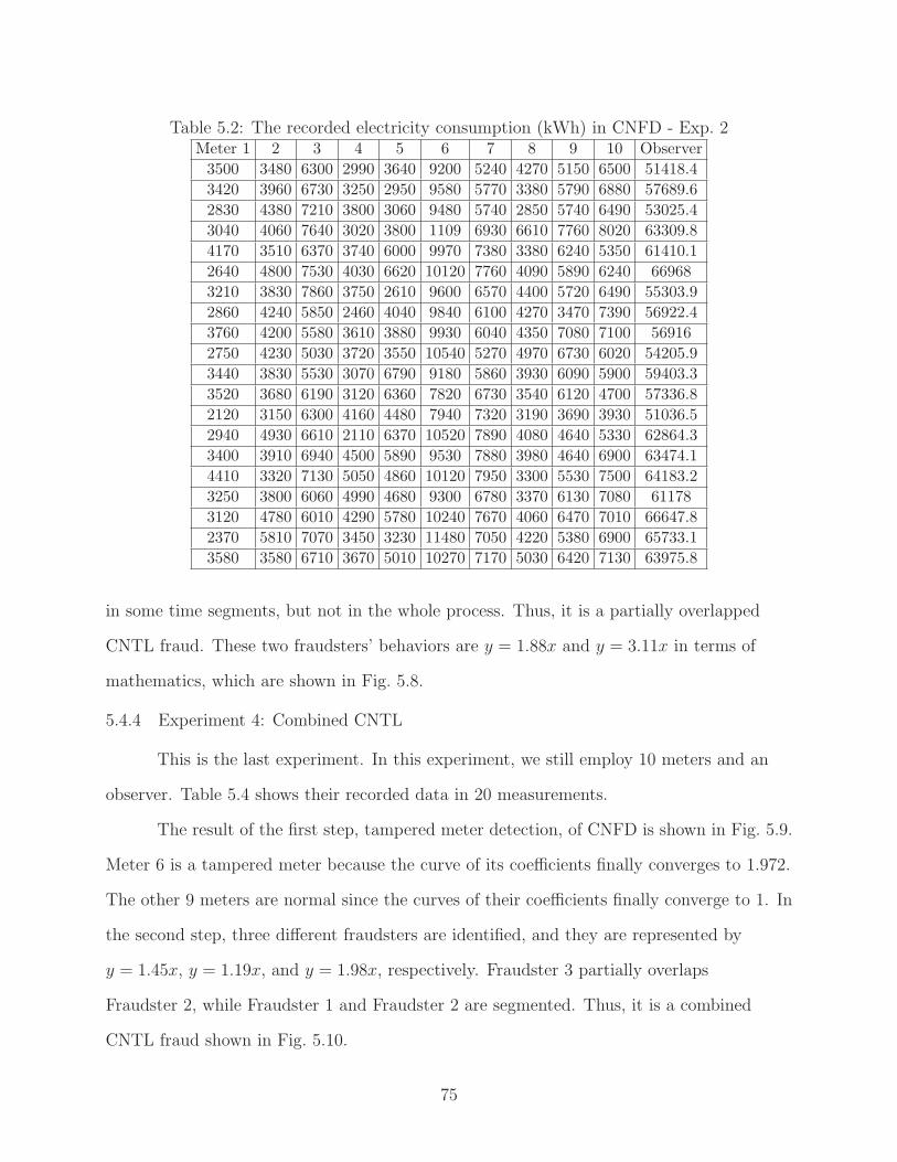
Table 5.2: The recorded electricity consumption (kWh) in CNFD - Exp. 2Meter 1 2 3 4 5 6 7 8 9 10 Observer
3500 3480 6300 2990 3640 9200 5240 4270 5150 6500 51418.4
3420 3960 6730 3250 2950 9580 5770 3380 5790 6880 57689.6
2830 4380 7210 3800 3060 9480 5740 2850 5740 6490 53025.4
3040 4060 7640 3020 3800 1109 6930 6610 7760 8020 63309.8
4170 3510 6370 3740 6000 9970 7380 3380 6240 5350 61410.1
2640 4800 7530 4030 6620 10120 7760 4090 5890 6240 66968
3210 3830 7860 3750 2610 9600 6570 4400 5720 6490 55303.9
2860 4240 5850 2460 4040 9840 6100 4270 3470 7390 56922.4
3760 4200 5580 3610 3880 9930 6040 4350 7080 7100 56916
2750 4230 5030 3720 3550 10540 5270 4970 6730 6020 54205.9
3440 3830 5530 3070 6790 9180 5860 3930 6090 5900 59403.3
3520 3680 6190 3120 6360 7820 6730 3540 6120 4700 57336.8
2120 3150 6300 4160 4480 7940 7320 3190 3690 3930 51036.5
2940 4930 6610 2110 6370 10520 7890 4080 4640 5330 62864.3
3400 3910 6940 4500 5890 9530 7880 3980 4640 6900 63474.1
4410 3320 7130 5050 4860 10120 7950 3300 5530 7500 64183.2
3250 3800 6060 4990 4680 9300 6780 3370 6130 7080 61178
3120 4780 6010 4290 5780 10240 7670 4060 6470 7010 66647.8
2370 5810 7070 3450 3230 11480 7050 4220 5380 6900 65733.1
3580 3580 6710 3670 5010 10270 7170 5030 6420 7130 63975.8
in some time segments, but not in the whole process. Thus, it is a partially overlapped
CNTL fraud. These two fraudsters’ behaviors are y = 1.88x and y = 3.11x in terms of
mathematics, which are shown in Fig. 5.8.
5.4.4 Experiment 4: Combined CNTL
This is the last experiment. In this experiment, we still employ 10 meters and an
observer. Table 5.4 shows their recorded data in 20 measurements.
The result of the first step, tampered meter detection, of CNFD is shown in Fig. 5.9.
Meter 6 is a tampered meter because the curve of its coefficients finally converges to 1.972.
The other 9 meters are normal since the curves of their coefficients finally converge to 1. In
the second step, three different fraudsters are identified, and they are represented by
y = 1.45x, y = 1.19x, and y = 1.98x, respectively. Fraudster 3 partially overlaps
Fraudster 2, while Fraudster 1 and Fraudster 2 are segmented. Thus, it is a combined
CNTL fraud shown in Fig. 5.10.
75

Figure 5.9: The result of the first step, tampered meter detection, of CNFD in Exp. 4. Itshows the converging process of the coefficients of 10 meters. The coefficient of Meter 6converges to 1.972 and the coefficients of other meters converge to 1 showing that Meter 6is the tampered meter.
Figure 5.10: The result of CNFD after the second step, fraudster differentiation, in Exp. 4.It shows that there is a CNTL fraud on Meter 6 which are committed by three fraudsters.
76
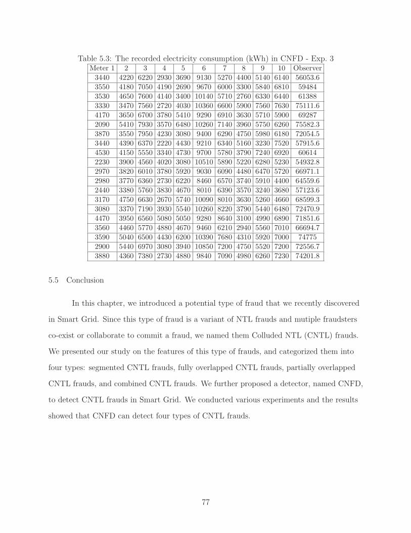
Table 5.3: The recorded electricity consumption (kWh) in CNFD - Exp. 3Meter 1 2 3 4 5 6 7 8 9 10 Observer
3440 4220 6220 2930 3690 9130 5270 4400 5140 6140 56053.6
3550 4180 7050 4190 2690 9670 6000 3300 5840 6810 59484
3530 4650 7600 4140 3400 10140 5710 2760 6330 6440 61388
3330 3470 7560 2720 4030 10360 6600 5900 7560 7630 75111.6
4170 3650 6700 3780 5410 9290 6910 3630 5710 5900 69287
2090 5410 7930 3570 6480 10260 7140 3960 5750 6260 75582.3
3870 3550 7950 4230 3080 9400 6290 4750 5980 6180 72054.5
3440 4390 6370 2220 4430 9210 6340 5160 3230 7520 57915.6
4530 4150 5550 3340 4730 9700 5780 3790 7240 6920 60614
2230 3900 4560 4020 3080 10510 5890 5220 6280 5230 54932.8
2970 3820 6010 3780 5920 9030 6090 4480 6470 5720 66971.1
2980 3770 6360 2730 6220 8460 6570 3740 5910 4400 64559.6
2440 3380 5760 3830 4670 8010 6390 3570 3240 3680 57123.6
3170 4750 6630 2670 5740 10090 8010 3630 5260 4660 68599.3
3080 3370 7190 3930 5540 10260 8220 3790 5440 6480 72470.9
4470 3950 6560 5080 5050 9280 8640 3100 4990 6890 71851.6
3560 4460 5770 4880 4670 9460 6210 2940 5560 7010 66694.7
3590 5040 6500 4430 6200 10390 7680 4310 5920 7000 74775
2900 5440 6970 3080 3940 10850 7200 4750 5520 7200 72556.7
3880 4360 7380 2730 4880 9840 7090 4980 6260 7230 74201.8
5.5 Conclusion
In this chapter, we introduced a potential type of fraud that we recently discovered
in Smart Grid. Since this type of fraud is a variant of NTL frauds and mutiple fraudsters
co-exist or collaborate to commit a fraud, we named them Colluded NTL (CNTL) frauds.
We presented our study on the features of this type of frauds, and categorized them into
four types: segmented CNTL frauds, fully overlapped CNTL frauds, partially overlapped
CNTL frauds, and combined CNTL frauds. We further proposed a detector, named CNFD,
to detect CNTL frauds in Smart Grid. We conducted various experiments and the results
showed that CNFD can detect four types of CNTL frauds.
77

Table 5.4: The recorded electricity consumption (kWh) in CNFD - Exp. 4Meter 1 2 3 4 5 6 7 8 9 10 Observer
2920 3590 6470 2300 3490 9550 5530 4110 5830 6310 54397.5
3560 3710 6980 3930 2650 9070 6280 2920 5440 6320 54941.5
3100 4540 7140 3160 3230 9600 6380 2210 6020 6540 56240
2660 4350 6860 3230 3540 10410 6800 6200 8210 7430 64374.5
3380 4430 6100 3060 5220 9330 7380 3800 6510 5510 56492.7
2240 5260 7360 4110 6740 10370 7270 4740 5820 6770 70842.6
3670 3500 7920 4300 2570 9590 6260 4040 6330 6850 64428.2
3000 4530 6250 2940 3760 9740 6500 4530 3280 7590 53970.6
4590 4600 5600 3560 4270 9230 5980 4130 6650 7140 57503.7
2920 4210 5150 3430 3190 10260 5460 4680 6910 5710 53869.4
3640 3260 6150 3270 6430 9200 5860 4740 6540 5630 63736
3050 3680 5430 3440 6470 8020 7190 3560 6610 4610 59919.6
2220 3140 5930 4180 4940 8550 6760 2890 3710 3700 54399
2720 4710 5990 2380 6340 10090 7620 3900 5160 4680 63478.2
3480 3870 7280 4670 5270 9500 8380 3980 5220 6920 67880
4228 3948 6678 5348 4780 10188 8088 3668 4818 7480 68976.4
3840 3750 6090 4710 4870 9570 6840 3110 6270 7350 65778.6
3740 5100 6410 4850 5570 9770 7430 4310 5670 6920 69344.6
3060 5520 7180 3630 3900 10590 6920 4240 5580 6480 67478.2
3630 3790 6820 3520 4580 9850 6670 5740 6130 7280 67663
78

CHAPTER 6
CONCLUSION
In this dissertation, we summarized our recent research on NTL fraud detection in
Smart Grid. We first introduced the background of Smart Grid and AMI communication
networks. Then, we introduced the research problem - NTL fraud detection including its
problem definition and attack model. We studied all the existing solutions that used to
address this problem and divided them into five categories. Based on the problems that we
found on these solutions, we further propose three novel detectors to solve these problems.
The proposed detectors are lightweight and non-traditional. They are built on numerical
analysis methods to model adversary behavior which are different from the traditional
IDS-based security solutions. They only need a small dataset and do not need detailed
energy consumption data which may cause privacy concerns. We presented the
experimental results to show the effectiveness of the three detectors. We analyzed the
performance of the three detectors theoretically and experimentally. Besides these three
detectors, we also published NTL fraud related research in the papers [20, 23, 24]. Some
other security related search papers that we published can be found in these
articles [22, 27, 30, 33, 37, 42, 63, 64].
In the future, we will study the conjecture of NFD and set up a series of
experiments to test its false alarm rate and efficiency in real-world applications. We will
further improve the stability of FNFD and validate its performance in the real applications.
My future research plan is three fold. First, lightweight and delay-tolerant authentication
scheme. Second, fog-computing-driven security analytic. Third, secure time
synchronization systems.
79

REFERENCES
[1] Runge’s phenomenon - tallinn university. (n.d.). available at:http://www.tlu.ee/ tonu/Arvmeet/Runge’s%20phenomenon.pdf.
[2] Average household electricity use around the world. available at:http://shrinkthatfootprint.com/average-household-electricity-consumption, 2010.
[3] Ansi c12.19-2012. available at: https://www.nema.org/Standards/ComplimentaryDocuments/C12-19-2012-Contents-and-Scope.pdf, 2012.
[4] Smart meter hacking tool released. available at:http://www.zdnet.com/article/smart-meter-hacking-tool-released/, 2012.
[5] Utility-scale smart meter deployments, plans, & proposals. availableat:http://www.edisonfoundation.net/iee/Documents/IEE SmartMeterRollouts 0512.pdf, May 2012.
[6] Emerging markets smart grid: Outlook 2015. availableat:http://www.northeast-group.com/reports/Brochure-Emerging%20Markets%20Smart%20Grid-Outlook%202015-Northeast%20Group.pdf,December 2014.
[7] X. Bai. Study of taylor formular approximation precision. College Mathematics,2(4):108–110, August 2016.
[8] R. Berthier and W. H. Sanders. Monitoring advanced metering infrastructures withamilyzer. Cyber-security of SCADA & industrial control systems, 2013.
[9] F. Biscarri, I. Monedero, C. Leon, and J. I. Guerrero. A mining framework to detectnon-technical losses in power utilities. In Proceedings of 11th International Conferenceon Enterprise Information System (ICEIS’09), 2009.
80

[10] I. Hakki Cavdarl. A solution to remote detection of illegal electricity usage via powerline communications. IEEE Transactions on Power Delivery, 19, October 2004.
[11] M. Comenetz. Calculus: The Elements. World Scientific, 2002.
[12] Breno C. Costa, Bruno. L. A. Alberto, Andre M. Portela, W. Maduro, and Esdras O.Eler. Fraud detection in electric power distribution networks using an ann-basedknowledge-discover process. International Journal of Artificial Intelligence &Applications (IJAIA), 4(6):11–23, November 2013.
[13] S.S.S.R. Depuru, L. Wang, and V. Devabhaktuni. Support vector machine based dataclassification for detection of electricity theft. In Proceedings of IEEE/PES PowerSystems Conference and Exposition (PSCE), pages 1–8, March 2011.
[14] Eduardo Werley S. dos Angelos, Osvaldo R. Saavedra, Omar A. Carmona Cortes, andAndre Nunes de Souza. Detection and identification of abnormalities in customerconsumptions in power distribution systems. IEEE Transactions on Power Delivery,26(4):2436–2442, October 2011.
[15] J. Gao, Y. Xiao, J. Liu, W. Liang, , and C. L. P. Chen. A survey ofcommunication/networking in smart grids. Future Generation Computer Systems,28(2):391–404, Febuary 2012.
[16] J. Gao, Y. Xiao, J. Liu, W. Liang, and C. L. P. Chen. A survey ofcommunication/networking in smart grids. (Elsevier) Future Generation ComputerSystems, 28(2):391–404, 2012.
[17] Jingcheng Gao, Jing Liu, Bharat Rajan, Rahul Nori, Bo Fu, Yang Xiao, Wei Liang,and C. L. Philip Chen. Scada communication and security issues. Security andCommunication Networks Security Comm, 7(1):175–194, 2014.
[18] D.J. Gaushell and H.T. Darlington. Supervisory control and data acquisition.Proceedings of the IEEE, 75(3):1645–1658, 2005.
[19] Georges Habrail and Alice Barard. Individual household electric power consumptiondata set. available at:https://archive.ics.uci.edu/ml/datasets/Individual+household+electric+power+consumption, 2012.
81

[20] Wenin Han and Yang Xiao. Big data security analytic for smart grid with fog nodes.In In Proceedings of the 9th International Conference on Security, Privacy andAnonymity in Computation, Communication and Storage (SpaCCS 2016), pages59–69, November 2016.
[21] Wenin Han and Yang Xiao. CNFD: A novel scheme to detect colluded non-technicalloss fraud in smart grid. In The 11th International Conference on WirelessAlgorithms, Systems, and Applications (WASA 2016), pages 47–55, August 2016.
[22] Wenin Han and Yang Xiao. CO2: A fault-tolerant relay node deployment strategy forthrowbox-based dtns. In In Proceedings of the 11th International Conference onWireless Algorithms, Systems, and Applications (WASA 2016), pages 37–46, August2016.
[23] Wenin Han and Yang Xiao. Combating TNTL: Non-technical loss fraud targetingtime-based pricing in smart grid. In The 2nd International Conference on CloudComputing and Security (ICCCS 2016), July 2016.
[24] Wenin Han and Yang Xiao. Non-technical loss fraud in advanced meteringinfrastructure in smart grid. In The 2nd International Conference on CloudComputing and Security (ICCCS 2016), 2016.
[25] Wenin Han and Yang Xiao. Privacy preserving for v2g networks in smart grid: Asurvey. Computer Communications, 91-92:17–28, 2016.
[26] Wenlin Han and Yang Xiao. NFD: A practical scheme to detect non-technical lossfraud in smart grid. In Proceedings of the 50th International Conference onCommunications (ICC’14), pages 605–609, June 2014.
[27] Wenlin Han and Yang Xiao. IP2DM for V2G networks in smart grid. In Proceedings ofthe 50th International Conference on Communications (ICC’15), pages 782–787, June2015.
[28] Wenlin Han and Yang Xiao. Design a fast non-technical loss fraud detector in smartgrid. (Wiley Journal of) Security and Communication Networks, October 2016.
[29] Wenlin Han and Yang Xiao. FNFD: A fast scheme to detect and verify non-technicalloss fraud in smart grid. In International Workshop on Traffic Measurements for
82

Cybersecurity (WTMC’16), DOI: http://dx.doi.org/10.1145/2903185.2903188, pages24–34, May 30 - June 3 2016.
[30] Wenlin Han and Yang Xiao. IP2DM: Integrated privacy-preserving data managementarchitecture for smart grid v2g networks. Wireless Communications and MobileComputing, September 2016.
[31] Wenlin Han and Yang Xiao. NFD: Non-technical loss fraud detection in smart grid.Computers & Security, November 2016.
[32] Wenlin Han and Yang Xiao. A novel detector to detect colluded non-technical lossfraud in smart grid. Computer Networks, October 2016.
[33] Wenlin Han, Wei Xiong, Yang Xiao, M. Ellabidy, A. V. Vasilakos, and Naixue Xiong.A class of non-statistical traffic anomaly detection in complex network systems. InProceedings of the 32nd International Conference on Distributed Computing SystemsWorkshops (ICDCSW’12), pages 640–646, June 2012.
[34] Monson H. Hayes. Recursive least squares. In Statistical Digital Signal Processing andModeling, chapter 9.4, page 154. Wiley, 1996.
[35] Shih-Che Huang, Yuan-Liang Lo, and Chan-Nan Lu. Non-technical loss detectionusing state estimation and analysis of variance. IEEE Transactions on Power Systems,28(3):2959–2966, August 2013.
[36] Paria Jokar, Nasim Arianpoo, and Victor C. M. Leung. A survey on security issues insmart grids. Security and Communication Networks, 9:262–273, June 2012.
[37] Julius Jow, Yang Xiao, and Wenlin Han. A survey of intrusion detection in smart grid.International Journal of Sensor Networks, 2017.
[38] G. Kalogridis, S.Z. Denic, T. Lewis, and R. Cepeda. Privacy protection system andmetrics for hiding electrical events. International Journal of Security and Networks,6(1):14–27, 2011.
[39] F. Li, B. Luo, and P. Liu. Secure and privacy-preserving information aggregation forsmart grids. International Journal of Security and Networks, 6(1):28–39, 2011.
83

[40] Chia-Hung Lin, Shi-Jaw Chen, Chao-Lin Kuo, and Jian-Liung Chen. Non-cooperativegame model applied to an advanced metering infrastructure for non-technical lossscreening in micro-distribution systems. IEEE Transactions on Smart Grid,5(5):2468–2469, September 2014.
[41] J. Liu, Y. Xiao, S. Li, W. Liang, and C. L. P. Chen. Cyber security and privacy issuesin smart grids. IEEE Communications Surveys & Tutorials, 14(4):981–997, FourthQuarter 2012.
[42] Jing Liu, Wenlin Han, and Yang Xiao. Enhancements of temporal accountability inmedical sensor networks. Ad hoc & sensor wireless networks, 2017.
[43] S. Ma, Y. Yang, Y. Qian, H. Sharif, and M. Alahmad. Energy harvesting for wirelesssensor networks: applications and challenges in smart grid. International Journal ofSensor Networks, 21(4):226–241, 2016.
[44] Patrick McDaniel and Sean W. Smith. Security and privacy challenges in the smartgrid. IEEE Security & Privacy, 7(3):75–77, 2009.
[45] Stephen McLaughlin, Brett Holbert, Saman Zonouz, and Robin Berthier. AMIDS: Amulti-sensor energy theft detection framework for advanced metering infrastructures.In Proceedings of the 2012 IEEE Third International Conference on Smart GridCommunications (SmartGridComm’12), pages 354–359, November 2012.
[46] N. Mohammad, A. Baru, and M.A. Arafat. A smart prepaid energy metering systemto control electricity theft. In Proceedings of the Int’l Conf. on Power, Energy andControl, pages 562–565, 2013.
[47] J. Mu, W. Song, W. Wang, and B. Zhang. Self-healing hierarchical architecture forzigbee network in smart grid application. International Journal of Sensor Networks,17(2):130–137, 2015.
[48] U.S. Department of Energy. The smart grid: an introduction. available at:http://energy.gov/oe/downloads/smart-grid-introduction-0. Accessed: 02/09/2016.
[49] A. Pasdar and S. Mirzakuchaki. A solution to remote detecting of illegal electricityusage based on smart metering. In Proceedings of the 2nd Int’l workshop on SoftComputing Applications, pages 163–167, 2007.
84
[50] Perumalraja Rengaraju, Shunmugham R. Pandian, and Chung-Horng Lung.Communication networks and non-technical energy loss control system for smart gridnetworks. In Proceedings of the 2014 IEEE Innovative Smart Grid Technologies - Asia(ISGT ASIA), pages 418–423, May 2014.
[51] Patil S, Gopal Pawaskar, and Kirtikumar Patil. Electrical power theft detection andwireless meter reading. Int’l Journal of Innovative Research in Science, Eng. andTechnology, 2:114–119, 2013.
[52] K. Silverstein. India and u.s. share energy woes: Stealing electricity. availableat:http://www.forbes.com/sites/kensilverstein/2012/08/05/india-and-u-s-share-energy-woes-stealing-electricity/,2012.
[53] SATEC Power Solutions. Accuracy class: a small s that makes a big difference.available at: http://www.satec-global.com/sites/default/files/ApplicationNote-Accuracy-Class-Dec2012.pdf,2012.
[54] M. Spivak. Calculus (3rd ed.). Houston, TX: Publish or Perish, 1994.
[55] R. Targosz. Electricity theft - a complex problem. available at:http://www.leonardo-energy.org/electricity-theft-complex-problem, July 2009.
[56] K. Tweed. Fbi finds smart meter hacking surprisingly easy. availableat:http://www.greentechmedia.com/articles/read/fbi-finds-smart-meter-hacking-surprisingly-easy/,2012.
[57] J.V. Wijayakulasooriya, D.M.I.S. Dasanayake, P.I. Muthukumarana, H.M.P.P.Kumara, and L.A.D.S.D. Thelisinghe. Remotely accessible single phase energymeasuring system. In Proceedings of the 1st Int’l Conf. on Industrial and InformationSystems, pages 304–309, 2006.
[58] Xiaofang Xia, Wei Liang, Yang Xiao, and Meng Zheng. BCGI: A fast approach todetect malicious meters in neighborhood area smart grid. In Proceedings of the 50thInternational Conference on Communications (ICC’15), pages 7228–7233, June 2015.
85
[59] Xiaofang Xia, Wei Liang, Yang Xiao, Meng Zheng, and Zhifeng Xiao.Difference-comparison-based approach for malicious meter inspection in neighborhoodarea smart grids. In Proceedings of the 50th International Conference onCommunications (ICC’15), pages 802–807, June 2015.
[60] Z. Xiao, Y. Xiao, and D. Du. Building accountable smart grids in neighborhood areanetworks. In Proceedings of the IEEE Global Telecommunications Conference 2011(GLOBECOM’11), pages 1–5, December 2011.
[61] Z. Xiao, Y. Xiao, and D. Du. Exploring malicious meter inspection in neighborhoodarea smart grids. IEEE Transactions on Smart Grid, 4(1):214–226, March 2013.
[62] Z. Xiao, Y. Xiao, and D. Du. Non-repudiation in neighborhood area networks forsmart grid. IEEE Communications Magazine, 51(1):18–26, January 2013.
[63] Junhan Yang, Bo Su, Chaoping Guo, Wenlin Han, and Yang Xiao. Provably securecl-kem based password-authenticated key exchange protocol. International Journal ofSensor Networks, 2017.
[64] Lei Zeng, Yang Xiao, Hui Chen, Bo Sun, and Wenlin Han. Computer operatingsystem logging and security issues: A survey. (Wiley Journal of) Security andCommunication Networks, October 2016.
86
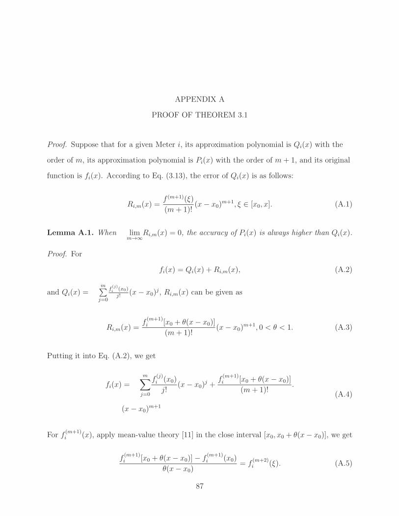
APPENDIX A
PROOF OF THEOREM 3.1
Proof. Suppose that for a given Meter i, its approximation polynomial is Qi(x) with the
order of m, its approximation polynomial is Pi(x) with the order of m+ 1, and its original
function is fi(x). According to Eq. (3.13), the error of Qi(x) is as follows:
Ri,m(x) =f (m+1)(ξ)
(m+ 1)!(x− x0)
m+1, ξ ∈ [x0, x]. (A.1)
Lemma A.1. When limm→∞
Ri,m(x) = 0, the accuracy of Pi(x) is always higher than Qi(x).
Proof. For
fi(x) = Qi(x) +Ri,m(x), (A.2)
and Qi(x) =m∑j=0
f(j)i (x0)
j!(x− x0)
j, Ri,m(x) can be given as
Ri,m(x) =f(m+1)i [x0 + θ(x− x0)]
(m+ 1)!(x− x0)
m+1, 0 < θ < 1. (A.3)
Putting it into Eq. (A.2), we get
fi(x) =m∑j=0
f(j)i (x0)
j!(x− x0)
j +f(m+1)i [x0 + θ(x− x0)]
(m+ 1)!.
(x− x0)m+1
(A.4)
For f(m+1)i (x), apply mean-value theory [11] in the close interval [x0, x0 + θ(x− x0)], we get
f(m+1)i [x0 + θ(x− x0)]− f
(m+1)i (x0)
θ(x− x0)= f
(m+2)i (ξ). (A.5)
87

Thus,
f(m+1)i [x0 + θ(x− x0)] = θ(x− x0)f
(m+2)i (ξ) + f
(m+1)i (x0). (A.6)
Put Eq. (A.6) into Eq. (A.4) to obtain:
fi(x) = Qi,(m+1)(x) +θf
(m+2)i (ξ)
(m+ 1)!(x− x0)
m+2. (A.7)
From Eq. (A.2), we get
fi(x) = Qi,(m+1)(x) +f(m+2)i [x0 + θ1(x− x0)]
(m+ 2)!(x− x0)
m+2,
0 < θ1 < 1.
(A.8)
Comparing Eqs. (A.7) and (A.8), the following can be obtained
θf(m+2)i (ξ)
(m+ 1)!(x− x0)
m+2 =f(m+2)i [x0 + θ1(x− x0)]
(m+ 2)!.
(x− x0)m+2.
According to [7], suppose x→ x0.
∵ f(m+2)i (x0) �= 0, and f
(m+2)i (x) is continuous,
∴ limx→x0
θ =1
m+ 2.
When x0 is in a sufficiently small neighborhood, θ ≈ 1m+2
, and
fi(x) ≈ Qi,m(x) +f(m+1)i (x0 +
x−x0
m+2)
(m+ 1)!(x− x0)
m+1. (A.9)
The right side of Eq. (A.9) is actually the approximation of fi(x) with m+ 1 order. That is
Pi(x) = Qi,m(x) +f(m+1)i (x0 +
x−x0
m+2)
(m+ 1)!(x− x0)
m+1, (A.10)
88
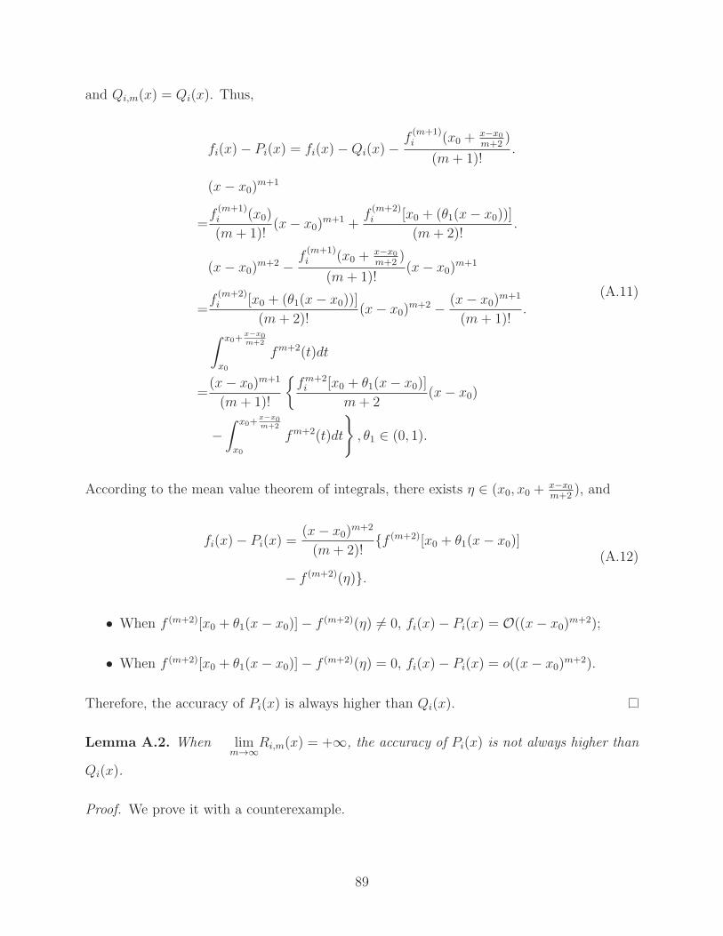
and Qi,m(x) = Qi(x). Thus,
fi(x)− Pi(x) = fi(x)−Qi(x)−f(m+1)i (x0 +
x−x0
m+2)
(m+ 1)!.
(x− x0)m+1
=f(m+1)i (x0)
(m+ 1)!(x− x0)
m+1 +f(m+2)i [x0 + (θ1(x− x0))]
(m+ 2)!.
(x− x0)m+2 − f
(m+1)i (x0 +
x−x0
m+2)
(m+ 1)!(x− x0)
m+1
=f(m+2)i [x0 + (θ1(x− x0))]
(m+ 2)!(x− x0)
m+2 − (x− x0)m+1
(m+ 1)!.
∫ x0+x−x0m+2
x0
fm+2(t)dt
=(x− x0)
m+1
(m+ 1)!
{fm+2i [x0 + θ1(x− x0)]
m+ 2(x− x0)
−∫ x0+
x−x0m+2
x0
fm+2(t)dt
}, θ1 ∈ (0, 1).
(A.11)
According to the mean value theorem of integrals, there exists η ∈ (x0, x0 +x−x0
m+2), and
fi(x)− Pi(x) =(x− x0)
m+2
(m+ 2)!{f (m+2)[x0 + θ1(x− x0)]
− f (m+2)(η)}.(A.12)
• When f (m+2)[x0 + θ1(x− x0)]− f (m+2)(η) �= 0, fi(x)− Pi(x) = O((x− x0)m+2);
• When f (m+2)[x0 + θ1(x− x0)]− f (m+2)(η) = 0, fi(x)− Pi(x) = o((x− x0)m+2).
Therefore, the accuracy of Pi(x) is always higher than Qi(x).
Lemma A.2. When limm→∞
Ri,m(x) = +∞, the accuracy of Pi(x) is not always higher than
Qi(x).
Proof. We prove it with a counterexample.
89

Consider the following function
fi(x) =2
2 + 33x2. (A.13)
1 0.5 0 0.5 10.4
0.2
0
0.2
0.4
0.6
0.8
1
x
f(x) =
2/(2
+33x
2 )
Order 2Order 3Order 5Order 9Original
Figure A.1: The curves of approximation polynomials with different orders of the samefunction fi(x) = 2
2+33x2 . A counter example to illustrate a higher order does not alwaysimprove accuracy.
Fig. A.1 shows its approximation polynomials with order 2, order 3, order 5, and
order 9, respectively. The order 5 polynomial, the red curve, is a better approximation
than the order 2, the green curve, and the order 3, the magenta curve. Most of the order 9
curve, the blue one, is closer to the original function than the order 5, the red curve.
However, it oscillates at the end of the interval, i.e. close to − 1 and 1. The reason is that
the upper bound for the approximation error grows to infinity with m [1].
fi(x)−Qi(x) =f (m+1)(ξ)
(m+ 1)!
m+1∏j=1
(x− xj), ξ ∈ [x0, x], (A.14)
90

and for some ξ ∈ (−1, 1),
max−1≤x≤1
|fi(x)− Pi(x)| ≤ max−1≤x≤1
f(m+1)i (x)
(m+ 1)!.
max−1≤x≤1
m+1∏j=1
(x− xj).
(A.15)
Thus,
limm→∞
(max
−1≤x≤1|fi(x)− Pi(x)|
)= +∞. (A.16)
Because of the oscillation, a meter’s polynomial of a higher order could be less accurate
than its polynomial of a lower order, especially when the range of the measured electricity -
x, is close to the oscillation range. Therefore, when limm→∞
Ri,m(x) = +∞, the accuracy of
Pi(x) is not always higher than Qi(x).
Based on Lemmas A.1 and A.2,
1. When limm→∞
Ri,m(x) = 0, the accuracy of Pi(x) is always higher than Qi(x);
2. When limm→∞
Ri,m(x) = +∞, the accuracy of Pi(x) is not always higher than Qi(x).
A polynomial with a higher order m does not always improve the accuracy of its
approximation. Theorem 3.1 has then been established.
91