Embed Size (px)
Citation preview
Noncommutative geometry and reality Alain Connes lnstitut des Hautes Etudes Scientijques, College de France, 35 Route de Chartres, F-91440 Bures-sur-Yvette, France
(Received 4 April 1995; accepted for publication 7 June 1995)
We introduce the notion of real structure in our spectral geometry. This notion is motivated by Atiyah’s KR-theory and by Tomita’s involution J. It allows us to remove two unpleasant features of the “Connes-Lott” description of the standard model, namely, the use of bivector potentials and the asymmetry in the Poincare duality and in the unimodularity condition. 0 1995 American Institute of Physics.
1. ON THE NOTION OF GEOMETRIC SPACE
The geometric concepts have first been formulated and exploited in the Framework of Eu- clidean geometry. This framework is best described using Euclid’s axioms (in their modern form by Hilbert’). These axioms involve the set X of points p E X of the geometric space as well as families of subsets: the lines and the planes for 3-dimensional geometry. Besides incidence and order axioms one assumes that an equivalence relation (called congruence) is given between segments, i.e., pairs of points @,q),p,q EX and also between angles, i.e., triples of points (a,O,b);a,O,b EX. These relations eventually allow us to define the length I(p.q)[ of a segment and the size K(a,O,b) of an angle. The geometry is uniquely specified once these two congruence relations are given. They of course have to satisfy a compatibility axiom: up to congruence a triangle with vertices a,O,b EX is uniquely specified by the angle Q(a,O,b) and the lengths of (a,O) and (0,b) (Fig. 1). Besides the completeness or continuity axiom, the crucial one is the axiom of unique parallel. The efforts of many mathematicians trying to deduce this last axiom from the others led to the discovery of non-Euclidean geometry.
One can describe non-Euclidean geometry using the Klein model or the Poincare model. In the Klein model, say for 2-dimensional geometry, the set X of points of the geometry is the interior of an ellipse (Fig. 2). The lines / are the intersections of Euclidean lines with X (Fig. 2) and the measurements of length and angles are given by
I(p,q)1=log(cross ratio(p,q;r,s)), (1.1)
where r,s are the points of intersection of the Euclidean line p,q with the ellipse, as shown in Fig. 2
Q(a,O,b)= & log (cross ratio(cr,P;&y)), (1.2)
where a, p are the Euclidean lines (0,a) and (0,b) and S,y are the (imaginary) Euclidean tangents to the ellipse passing through the point 0.
In the Poincare (disk) model the set X is the interior of the unit disk in the Euclidean plane. The lines are the intersections of Euclidean circles orthogonal to the boundary of the disk (Fig. 3) with the set X. The angles are the usual Euclidean angles between the circles and the distance between two points (p,q) is given by
I(p,q)l=log cross ratio(p,q;r,s), (1.3)
where r,s are as shown in Fig. 3.
6194 J. Math. Phys. 36 (ii), November 1995 0022-2488/95/36(11)/6194/36/$6.00
0 1995 American Institute of Physics
Downloaded 22 Feb 2007 to 129.132.239.8. Redistribution subject to AIP license or copyright, see http://jmp.aip.org/jmp/copyright.jsp

Alain Connes: Noncommutative geometry and reality 6195
b
FIG. 1.
The introduction by Descartes of coordinates in geometry was at first an act of violence (cf. Ref. 2). In the hands of Gauss and Riemann it allowed one to extend considerably the domain of validity of geometric ideas. In Riemannian geometry the space Xn is an n-dimensional manifold. Locally in X a point p is uniquely specified by giving n real numbers x’,...,x~ which are the coordinates of p. The various coordinate patches are related by diffeomorphisms. The geometric structure on X is prescribed by a (positive definite) quadratic form,
g&xc” dx’,
which specifies the length of tangent vectors Y E T,(X), Y = YP”d,, by
11 Y(12=g,,Y~Y”.
This allows, using integration, to define the length of a path r(t) in X, t E [0, l] by
(1.4)
(1.5)
Length y= (1.6)
The analog of the lines of Euclidean or non-Euclidean geometry are the geodesics. The analog of the distance between two points p,q E X is given by the formula,
d(p,q)=Inf Length(y), (1.7)
where y varies among all paths with yfO)=p, fil)=q (Fig. 4). The obtained notion of “Riemann- ian space” has been so successful that it has become the paradigm of geometric space. There are
FIG. 2
J. Math. Phys., Vol. 36, No. 11, November 1995 Downloaded 22 Feb 2007 to 129.132.239.8. Redistribution subject to AIP license or copyright, see http://jmp.aip.org/jmp/copyright.jsp

6196 Alain Connes: Noncommutative geometry and reality
FIG. 3.
two main reasons behind this success. On the one hand this notion of Riemannian space is general enough to cover the above examples of Euclidean and non-Euclidean geometries and also the fundamental example given by space-time in general relativity (relaxing the positivity condition Of (4)).
On the other hand it is special enough to still deserve the name of geometry, the point being that through the use of local coordinates all the tools of the differential and integral calculus can be brought to bear. As an example let us just mention the equation of geodesics
d’x’ dxj dxk dt’ = rjk dt dt (1.8)
which yields Newton’s law in a given gravitational potential V provided the goo= - 1 of flat space-time is replaced by -(I +2V) (cf. Ref. 3 for a more precise statement).
Besides its success in physics as a model of space-time, Riemannian geometry plays a key role in the understanding of the topology of manifolds, starting with the Gauss Bonnet theorem, the theory of characteristic classes, index theory, and the Yang Mills theory.
Thanks to the recent experimental confirmations of general relativity from the data given by binary pulsars4 there is little doubt that Riemannian geometry provides the right framework to understand the large scale structure of space-time.
The situation is quite different if one wants to consider the short scale structure of space-time. We refer to Refs. 5 and 6 for an analysis of the problem of the coordinates of an event when the scale is below the Planck length. In particular there is no good reason to presume that the texture of space-time will still be the 4-dimensional continuum at such scales.
FIG. 4.
J. Math. Phys., Vol. 36, No. 11, November 1995
Downloaded 22 Feb 2007 to 129.132.239.8. Redistribution subject to AIP license or copyright, see http://jmp.aip.org/jmp/copyright.jsp

Alain Connes: Noncommutative geometry and reality 6197
In this paper we shall propose a new paradigm of geometric space which allows us to incor- porate completely different small scale structures. It will be clear from the start that our framework is general enough. It will of course include ordinary Riemannian spaces but it will treat the discrete spaces on the same footing as the continuum, thus allowing for a mixture of the two. It also will allow for the possibility of noncommuting coordinates.6 Finally it is quite different from the geometry arising in string theory but is not incompatible with the latter since supersymmetric conformal field theory gives a geometric structure in our sense whose low energy part can be defined in our framework7 and compared to the target space geometry.
It will require the most work to show that our new paradigm still deserves the name of geometry. We shall need for that purpose to adapt the tools of the differential and integral calculus to our new framework. This will be done by building a long dictionary which relates the usual calculus (done with local differentiation of functions) with the new calculus which will be done with operators in Hilbert space and spectral analysis, commutators.... The first two lines of the dictionary give the usual interpretation of variable quantities in quantum mechanics as operators in Hilbert space. For this reason and many others (which include integrality results) the new calculus can be called the quantized calculus’ but the reader who has seen the word “quantized” overused so many times may as well drop it and use “spectral calculus” instead.
Let us now first define a general framework for spectral geometry. Dejinition 1: A spectral triple (~6, 38 D) is given by an involutive algebra of operators &L% in
a Hilbert space X‘ and a selfadjoint operator D = D” in 23 such that
a) The resolvent (D-X)-‘, AeW ofD is compact. /?) The commutators [D,a]=Da - aD are bounded, for any a ~~4:.
Furthermore, we shall say that such a triple is even if we are given a Z/2 grading of the Hilbert space .Y, i.e., an operator y in .%‘, y= p, $= 1 such that
ya=ay, VaE,&, Dy=-yD. (1.9)
Otherwise we shall say that the triple is odd. Before we give examples of spectrally defined geometric spaces let us make a number of
small comments on Definition 1. The algebra . 4 is an algebra of operators in %‘. Thus each element a E -4 is a (bounded)
operator in .k” and,
a,bE,&, h,,u*.EWjXa+,ubE,&, a,bE&*abE,,i%, aE&*a*E.&, (1.10)
where the third condition, . *%=.&* means that ,f% is involutive for the involution * given by the adjoint of operators,
(W”‘17)=(%rl)7 677EZ. (1.11)
We do not necessarily assume that S,& is stable by multiplication by complex numbers, though it is in most examples.
The algebra L rc! plays the role of the algebra of coordinates on the space X we are considering. In the commutative case, i.e., if
ab=ba, Va,b E.&:, (1.12)
then the space X is the spectrum of the C*-algebra ,% obtained as the norm closure of ..A in the algebra of bounded operators in Z for the norm,
IITIl=Sup{llTSll;II~I(~ 11. (1.13)
J. Math. Phys., Vol. 36, No. 11, November 1995 Downloaded 22 Feb 2007 to 129.132.239.8. Redistribution subject to AIP license or copyright, see http://jmp.aip.org/jmp/copyright.jsp

6198 Alain Connes: Noncommutative geometry and reality
This spectrum X is defined abstractly as the space of characters of .A, i.e., of * homomorphisms x: &-+C, i.e., of maps from .,b to C which preserve the relations (10). When ,A contains {Xl; X EC} the space X of characters, endowed with the topology of simple convergence,
xa+x iff x,(a)-+x(a) ifaEA (1.14)
is a compact space and by Gelfand’s theorem one has the canonical isomorphism
A= C(X), (1.15)
which to each a E ,% assigns the function a(x) =x(a), VXEX. To get a more concrete picture of X let us assume to simplify that the algebra ,A is generated by N-commuting self-adjoint elements x ,...,xN. Then X is identified with a compact subset of RN by the map, 1
X~X4X(X’) ,...,/y(XN)) ERN (1.16)
and the range of this map is the joint spectrum of x’,...,xXN. The notion of joint spectrum of N-commuting self-adjoint operators is quite simple. When 38 is finite dimensional, one takes unit vectors (ES?, 1141=1, h’ h w IC are eigenvectors for all the x P. To any such 5 there corresponds the N-uple of real numbers
(A’),= ,,...,N; x’&= Apt* (1.17)
The joint spectrum is just the set of all such N-uples when 5 varies among common eigenvectors. The infinite dimensional case is analogous with a suitable use of e’s to say that k=(X/*>,, I,,,,,N is an approximate eigenvalue.
Now when the algebra .A is no longer commutative the above picture of an associated compact space X becomes more subtle. Certainly .A? will contain commuting self-adjoint elements
I x ,...,xN as above, but these cannot generate ,& since the latter is not commutative. The simplest example of what happens in the noncommutative case is provided by the algebra ~8 of 2X2 matrices,
-A5=M2(C)={[aij]; i,j= 1,2, CZijEC}. (1.18)
The subalgebra of diagonal matrices,
s=[ [; j; LP.c)? (1.19)
is commutative and its spectrum X is a two point set given by the characters
xl[; ;]=A, x,[; ;]=p. These two characters extend as pure states (in the quantum mechanical terminology) of the algebra .-+5 as follows,
(1.20)
The basic new feature created by noncommutativity is the equivalence of the irreducible repre- sentations of ,d associated to the pure states gt and x2. This equivalence is provided by the off diagonal matrix
J. Math. Phys., Vol. 36, No. 11, November 1995
Downloaded 22 Feb 2007 to 129.132.239.8. Redistribution subject to AIP license or copyright, see http://jmp.aip.org/jmp/copyright.jsp

Alain Connes: Noncommutative geometry and reality 6199
0 1 u=l o’ [ 1 (1.21)
whose effect is to interchange 1 and 2. Thus the naive picture that one can keep in mind in the noncommutative case is that the points
of the space X are now replaced by the pure states of ,% together with the equivalence relation
CPI-(~2 iff =qp1-~q29 (1.22)
where rrcp is the irreducible representation of ,I;! associated to cp and - means unitary equivalence of representations.
We refer to Ref. 9 for these general notions on C*-algebras. One should not attribute too much value to this naive picture but remember that in the noncommutative case one is dealing with a space together with an equivalence relation rather than a space alone.
The operator D is by hypothesis a self-adjoint operator in .F and has discrete spectrum, given by eigenvalues X, E R which form a discrete subset of R. This follows from the hypothesis cy) and is just a reformulation of e). The pair given by the Hilbert space .% and the unbounded self- adjoint operator D is entirely characterized by the subset with multiplicities
SPD={XEW; 3,.$~.%?, t#O, 0.$=X6}, (1.23)
where we let m(X)=dim{tE*, 0,$=X,$} be th e multiplicity of h. In the even case the equality (9) shows that Sp D is even, i.e., m(-X)=m(X) for all XEW.
Two pairs, (Y,, D,), (ZZ, D2) which have the same eigenvalue list are unitarily equivalent and conversely. Moreover given an arbitrary proper eigenvalue list (A,), with finite multiplicities there exists an obvious corresponding pair (.%‘,D).
The notion of dimension of the spectral triple (<‘g, 2, D) is governed by the growth of the eigenvalues X, . This will become clearer when we dispose of the quantized calculus but we can already state that
c AESPD m(X)IXI-d<mjDimension of triple<d. (1.24)
The tractable infinite dimensional case is governed by the @summability condition
c m(X)ePx2<m. AsSpD
In fact as we shall see the correct notion of dimension of spectral triples is not given by a single number but by a subset CCQ: of the complex numbers. The condition (24) just implies the following inclusion,
CC{z EC; Re zsd}. (1.26)
This dimension spectra accounts for the obvious possibility of taking the union of two spaces of different dimensions as well as for noninteger (fractal) dimension and complex dimension.
Assuming (24) the condition p) of Definition 1 gives the upper bound d on the dimension of the joint spectrum of commuting selfadjoint elements of ,.1. It thus governs the visible dimension of the space we are dealing with.
Let us end these general comments by observing that in Definition 1 we do not have to be very careful in defining the algebra ,,g, only its weak closure s 04” does matter. The point is that the
J. Math. Phys., Vol. 36, No. 11, November 1995 Downloaded 22 Feb 2007 to 129.132.239.8. Redistribution subject to AIP license or copyright, see http://jmp.aip.org/jmp/copyright.jsp

6200 Alain Connes: Noncommutative geometry and reality
various degrees of regularity of elements of -4 such as Lipschitz, C” and real analytic only use the knowledge of ..&’ and D: Let S be the densely defined derivation given by
S(T)=IDIT-TIDI, (1.27)
where IDI is the positive square root of D2. The derivation S is the generator of the one parameter group of automorphisms of Z(.%), the algebra of bounded operators in .iyi, given by
a,(T)=e islDlre-islDje (1.28)
Of course in general this group does not leave the algebra ~6” globally invariant but the various regularities are nevertheless well defined as follows:
a E -4” is Lipschitz iff [D,a] is bounded. (1.29)
a of class C” (resp. Co) iff s-+ a,(a) is Cm (resp. CO).
Thus a is of class C” iff it belongs to n, Dom 8, the intersection of the domains of all powers of 6.
An isometry of a spectral triple (.,4X58) is given by a unitary operator U in .F such that
UDU”=D, U,,b”U” = J‘#‘. (1.30)
It of course preserves the above notions of smoothness and hence the corresponding subalgebras of .&‘.
The isometries form a group and this group endowed with the * strong topology is a compact group in full generality of spectral triples. At this point it is important to mention that Definition 1 as such only covers compact spaces. To handle locally compact spaces one allows the algebra L ,r! to be non unital, i.e., one allows that the identity operator does not belong to %I%, and one replaces 4 by
a’) a( D - A) -’ is compact for any a E A?.
This minor modification allows to treat locally compact spaces as well. After these general pre- liminaries we shall now give two examples. The first example will simply show that a Riemannian spin manifold M defines a canonical spectral triple as follows:
We let X be the Hilbert space L2(M,S) of square integrable sections of the spinor bundle S on M associated to the spin structure. The algebra J% of functions on M acts in ~8 by multipli- cation
(1.31)
The operator D is the Dirac operator, a self-adjoint differential operator of order 1, whose main property for our concern is that its principal symbol is given by
IIDA = ~(4% (1.32)
where y is the Clifford multiplication, yT,* XS, --+S, for any p EM and df is the differential of f. In particular, using (32) one checks that a measurable function f~ ,A” is Lipschitz iff the operator [D,f] is bounded in .%.
Moreover, the Lipschitz norm off is equal to the operator norm of [of] and we thus obtain the following:
J. Math. Phys., Vol. 36, No. 11, November 1995
Downloaded 22 Feb 2007 to 129.132.239.8. Redistribution subject to AIP license or copyright, see http://jmp.aip.org/jmp/copyright.jsp

Alain Connes: Noncommutative geometry and reality 6201
Proposition 2: Let (.,+4.3fD) be the Dirac spectral triple associated to a Riemannian spin manifold M. Then the locally compact space M is the spectrum of the commutative C”-algebra norm closure of
.A= {a E A”; [ D,a] bounded}
bvhile the geodesic distance on M (given by formula (7)) is
The formula given in Proposition 2 for the geodesic distance between two points is of a quite different kind than (7) in that it replaces an infimum over arcs, i.e., maps from [O,l] to the space we are dealing with, by a supremum involving coordinates or functions on our space, i.e., maps from our space to C. It is this formula which makes sense in our context and as we shall see shortly it applies immediately to discrete spaces where points cannot be connected by arcs.
At this point Proposition 2 shows that we did not lose any information in trading the Rie- mannian space M for the associated spectral triple, but we shall see when we dispose of the quantized calculus that the fundamental concepts which allow us to pass from the local to the global in Riemannian geometry, as well as those of gauge theory are available in the much greater generality of (finite dimensional) spectral triples.
Let us now describe very simple jnite spaces. The simplest is the space X consisting of two points a,b so that the algebra ,R is the algebra CM whose elements f are given by a pair of complex numbers f(a), f(b) while
(1.33)
To obtain a spectral triple we need a representation of .A in a Hilbert space 3 and an operator D =D* in .k: We let X=C@C in which the algebra ,& acts by diagonal matrices,
f-["b"' fill.
while the operator D is given by an off diagonal matrix
0 P D= [ 1 P 0’
pu>O.
The commutator [Df] is given by the matrix
[
0 CD,fl=
Af(b)-f(a))
-df(b)-f(a)) 0
and one sees that
(1.34)
(1.35)
(1.36)
(1.37)
gives a nonzero finite distance between a and b. If we introduce multiplicity in the representation (34) and replace ,u by a matrix then (37) gives
d(a,b)= l/X, A = largest eigenvalue of IpI. (1.38)
Let us now give a short list of examples of finite dimensional spectral triples referring to Refs. 8 and 10 for their construction.
J. Math. Phys., Vol. 36, No. 11, November 1995
Downloaded 22 Feb 2007 to 129.132.239.8. Redistribution subject to AIP license or copyright, see http://jmp.aip.org/jmp/copyright.jsp
6202 Alain Connes: Noncommutative geometry and reality
(1) Riemannian mantfolds (with some variations allowing for Finsler metrics and also for the replacement of (DI by ID]“, o~]O,l]).
(2) Manifolds with singularities. Using the work of J. Cheeger on conical singularities. In fact, the spectral triples are stable under the operation of “coning,” which is easy to formulate alge- braically.
(3) Discrete spaces and theirproduct with manifolds (as in the discussion in Ref. 8 of the standard model). The spectral triples are of course stable under products.
(4) Cantor sets. Their importance lies in the fact that they provide examples of dimension spectra which contain complex numbers.
(5) Nilpotent discrete groups. The algebra .A is the group ring of the discrete group F, and the nilpotency of F is required to ensure the finite-summability condition D- ’ E&~,“‘. We refer to Ref. 8 for the construction of the triple for subgroups of Lie groups.
(6) Transverse structure for foliations. This example, or rather the intimately related example of the DSfS-equivariant structure of a manifold is treated in detail in Ref. 10.
These examples show that the notion of spectral triple is fairly general. The spaces involved do not fully qualify yet as geometric spaces because we did not yet formulate algebraically what it means to be a manifold. As we shall see this will be achieved by the forthcoming notion of real structure on a spectral triple, i.e., an antilinear involution J on .Z satisfying suitable commutator relations. To explain the conceptual meaning of this notion we first need to recall classical results from the theory of ordinary manifolds in particular those of D. Sullivan, which exhibit the central role played by the KO-homology orientation of a manifold.
The classical notion of manijold. A d-dimensional closed topological manifold X is a compact space locally homeomorphic to open sets in Euclidean space of dimension d. Such local homeo- morphisms are called charts. If two charts overlap in the manifold one obtains an overlap homeo- morphism between open subsets of Euclidean space. A smooth (resp. PL...) structure on X is given by a covering by charts so that all overlap homeomorphisms are smooth (resp. PL...). By definition a PL homeomorphism is simply a homeomorphism which is piecewise linear.
Smooth manifolds can be triangulated and the resulting PL structure up to equivalence is uniquely determined by the original smooth structure. We can thus write:
Smooth- PL*Top. (1.39)
The above three notions of smooth, PL, and Topological manifolds are compared using the respective notions of tangent bundles. A smooth manifold X possesses a tangent bundle TX which is a real vector bundle over X. The stable isomorphism class of TX in the real K-theory of X is classified by the homotopy class of a map:
X-+BO. (1.40)
Similarly a PL (resp. Top) manifold possesses a tangent bundle but it is no longer a vector bundle but rather a suitable neighborhood of the diagonal in XXX for which the projection (x,y)-+x on X defines a PL (resp. Top) bundle. Such bundles are stably classified by the homotopy class of a natural map:
X+BPL (resp. BTop). (1.41)
The implication (39) yields natural maps:
BO+BPL+BTop (1.42)
and the nuance between the three above kinds of manifolds is governed by the ability to lift up to homotopy the classifying maps (41) for the tangent bundles. (In dimension 4 this statement has to
J. Math. Phys., Vol. 36, No. 11, November 1995
Downloaded 22 Feb 2007 to 129.132.239.8. Redistribution subject to AIP license or copyright, see http://jmp.aip.org/jmp/copyright.jsp

Alain Connes: Noncommutative geometry and reality 6203
be made unstably to go from Top to PL). It follows for instance that every PL manifold of dimension d<7 possesses a compatible smooth structure. Also for d>5, a topological manifold Xd admits a PL structure iff a single topological obstruction SeH4(X,a2) vanishes.
For d =4 one has Smooth= PL but topological manifolds only sometimes possess smooth structure (and when they do they are not unique up to equivalence) as follows from the works of Donaldson and Freedman.
The KO-orientation of a manifold. Any finite simplicial complex can be embedded in Euclid- ean space and has the homotopy type of a manifold with boundary. The homotopy types of manifolds with boundary is thus rather arbitrary. For closed manifolds this is no longer true and we shall now discuss this point.
Let X be a closed oriented manifold. Then the orientation class px EH,(X,Z)=Z defines a natural isomorphism:
(1.43)
which is called the Poincari duality isomorphism. This continues to hold for any space Y homo- topic to X since homology and cohomology are invariant under homotopy.
Conversely let X be a finite simplicial complex which satisfies Poincare duality (43) for a suitable class ,ux , then X is called a Poincard complex. If one assumes that X is simply connected (n,(X)=(e)), then (Ref. 11) there exists a unique up to fiber homotopy equivalence, spherical
fibration ELX over X (the fibers p-‘(b), b E X have the homotopy type of a sphere) which plays the role of the stable tangent bundle when X is homotopy equivalent to a manifold. Moreover, in the simply connected case and with d =dim X25, the problem of finding a PL manifold in the homotopy type of X is the same as that of promoting this spherical fibration to a PL bundle. There are, in general, obstructions for doing that, but a key result of D. Sullivan [ICM, Nice, 19701 asserts that after tensoring the relevant Abelian obstruction groups by Z[J, a PL bundle is the same thing as a spherical fibration together with a KO orientation. This shows first that the characteristic feature of the homotopy type of a PL manifold is to possess a KO orientation
VXE KO,tX), (1.44)
which defines a Poincare duality isomorphism in real K theory, after tensoring by 2[1/2]:
(1.45)
Moreover, it was shown that this element V, E KO,(X) describes all the invariants of the PL manifolds in a given homotopy type, provided the latter is simply connected and all relevant Abelian obstruction groups are tensored by a[;]. Among these invariants are the rational Pontr- jagin classes of the manifold. For smooth manifolds they are the Pontrjagin classes of the tangent vector bundle, but in general they are obtained from the Chern character of the KO orientation class vx . These classes continue to make sense for topological manifolds and are homeomorphism invariants thanks to the work of S. Novikov.
We can thus assert that, in the simply connected case, a closed manifold is in a rather deep sense more or less the same thing as a homotopy type X satisfying Poincard duality in ordinary homology together with a preferred element vx~ KO,(X) which induces Poincare duality in KO theory tensored by 2[1/2]. In the nonsimply connected case one has to take in account the equi- variance with respect to the fundamental group rri(X)=F acting on the universal cover r?.
Both K-homology and KO-homology have a beautiful operator theoretic interpretation due to Atiyah, Brown, Douglas, Fillmore, and Kasparov, which is at the origin of the notion of spectral triple. The key definition, which improves on the description of Poincare duality of Ref. 8 is based on KR-homology and is the following refinement on the notion of spectral triple. Real structure on a spectral triple.
J. Math. Phys., Vol. 36, No. 11, November 1995 Downloaded 22 Feb 2007 to 129.132.239.8. Redistribution subject to AIP license or copyright, see http://jmp.aip.org/jmp/copyright.jsp
6204 Alain Connes: Noncommutative geometry and reality
DeJLinition 3: Let (.&X0) be an even spectral triple. A real structure of mod 8 dimension 2k is an antilinear isometty J in .%f such that:
a) JD=DJ, J2=6, Jy=e’yJ. /3) For any a E .A the operators a and [D,a] commute with J&J*.
Here, E, E’ are equal to t 1 with values depending on 2k modulo 8, according to the following table:
d=O 2 4 6
E 1 -1 -1 1 E’ 1 -1 1 -1
(1.46)
Note that since J is an isometry one has J* = J- ’ = eJ. Condition /I) is a key condition motivated by Tomita’s theorem which for a von Neumann
algebra with cyclic and separating vector in Hilbert space SY constructs an antilinear involution J such that J(algebra)J* =commutant of the algebra.
‘Ibis condition also says that D is an operator of “order 1” (cf. Ref. 8). There is an obvious likeliness between Definition 3 and Atiyab’s KR theoryi or rather the
dual KR homology as defined by Kasparov.13 Before we clarify this relation we just mention an equivalent definition of a real structure of
mod 8 dimension IZ (not necessarily even). One lets C,,, be the real Clifford algebra (cf. Ref. 13) with p Dirac matrices $ of square 1 and 4 of square - 1, y,: all anticommuting pairwise, and with involution given by
(y,?)*=+ (1.47)
Let then (A, .Zc, D,) be an even spectral triple with an involutive representation r of C,,, in 2 which commutes with .t%l and anticommutes with D, and y
r( y,‘) E&3’ Vj, +f)D=-DTT(+, +,:)y=--yrr(y,‘). (1.48)
Let then J be an antilinear isometry in X satisfying 3p) as well as,
JD,= D,J, J2= 1, Jy= rJ, JTT( $)J= T( $). (1.49)
One checks that such triples correspond canonically, if p - q is even, to the real spectral triples of dimension p-q mod 8 of Definition 3. We leave the odd case as an exercise.
Let J be a real structure on a spectral triple (&.%fD) of mod 8 dimension 2k then the commutation relation 3/?) allows to endow .X with the following structure of &-bimodule:
atb=aJb*J*t Va,bEJA, YES. (1.50)
In other words the Hilbert space 3 is a module over the tensor product &G&,@ of &S by the opposite algebra &),
(1.51)
We then endow &@& with the antilinear involution
J. Math. Phys., Vol. 36, No. 11, November 1995
Downloaded 22 Feb 2007 to 129.132.239.8. Redistribution subject to AIP license or copyright, see http://jmp.aip.org/jmp/copyright.jsp

Alain Connes: Noncommutative geometry and reality 6205
7-(u%b”)=b*%(a*)o (52)
and one can check that one thus obtains an element cy of KR2k-homology for J&Q@ with involution 7. (Using the Clifford algebras C,,, as above, the operator F =Sign D and Kasparov’s definition of KR-homology.)‘” (The converse is not true since 3p) also involves the commutators [D,a] ,a E s 4). This KR-homology class yields in particular a Poincard duality map,
K*(.A)tK2k-*(./@) (1.53)
from K-cohomology to K-homology, by the Kasparov cup product with a,
XEK*(<R)+X@,~~~EK *k-*(A). (1.54)
The natural bilinear map Ko(.~d)XKo(~~)+Ko(~R@.~~) given by e,f+e@p at the level of idempotents, together with the Fredholm index pairing:
Ind D
K,(Y&J@) t Z
thus determine a bilinear form on K,(A) with values in Z. This form is symmetric in dimension ~0 mod 4 and antisymmetric in dimension ~2 mod 4 and plays the role of the signature in our context.
A complete description of Poincare duality also involves the existence of the inverse of LY, given by a KR-cohomology class p for ..&x& (cf. Ref. 8) but we have not yet found the exact role of this class, or rather of a specific cocycle representative of this class, in the general theory.
The spectral triple (< +&.X D) associated to the Dirac operator on a spin Riemannian manifold M admits a canonical real structure in the above sense. In the even dimensional case the antilinear isometry J is given by
(JcxP)=c5(P) VPEM, (1.55)
where C is the charge conjugation operator. The values of C* = E and of E’ such that C y= E’ yC are given by the above table (46).
There is a straightforward notion of product of two real spectral triples and the mod 8 dimensions add. For instance if (. d2, .X2, D,, J2) is of mod 8 dimension 0 one obtains,
:d=.,d1@.&2, %=%,C3.%2, D=D,@l++,gD2, J=J,%J~, (1.56)
which clearly has the same mod 8 dimension as the first triple. After developing in the next section a calculus of infinitesimals which will be our substitute for the usual differential and integral calculus, we shall describe a finite geometry whose product with the ordinary continuum will account for all the experimental information about the fine structure at small scale of our space- time (-( 100 Gev)-‘) embodied in the Lagrangian of the standard model of electroweak and strong interactions.
Before we embark in that we shall describe a simple example of a highly noncommutative geometry in the above sense and a small variant of Definition 3.
The 2-dimensional noncommutative torus ‘I’:. In the spectral triple (,&.Z D) the algebra -1% of operators in .p will generate afactor of type II, and the antilinear isometry J will be, up to a trivial modification, the Tomita involution.
Let us take the notations of Ref. 8, p. 580. Thus ,$=,/I, is the irrational rotation algebra where 0 is an irrational number. We let r. be the canonical normalized trace on .dO and as in Ref. 8 we let ,~‘=L2(..,~!e,70),.~=.~~~ being Z/2 graded by
J. Math. Phys., Vol. 36, No. 11, November 1995 Downloaded 22 Feb 2007 to 129.132.239.8. Redistribution subject to AIP license or copyright, see http://jmp.aip.org/jmp/copyright.jsp

6206 Alain Connes: Noncommutative geometry and reality
1 0 7’0 -1’ 1 I
while b&e acts on the left in a diagonal way. The operator D is (cf. Ref. 8), 0 d D= [ 1 d* 0’
(1.57)
in terms of the basic derivations 4 of L&0. With these notations, let Jo be the Tomita involution on L.*(J%~,~~), given by the formula
Jou=a* ‘daEAo. (1.58)
By construction Jo is an antilinear isometric involution of * which transforms the left action of .A, into the right one by the automorphism
a-+Joa*Jo of ~6~ with .A;.
The formula for the real structure J on the above spectral triple is then the following
(1.59)
J= (1.60)
One checks that the conditions of Definition 3 are fulfilled with dimension equal to 2 modulo 8. When we shall come to gauge theories this last example will be quite interesting for 8
irrational since then, unlike in the commutative case, the adjoint action
(u,++u&*=uJuJ*~ (1.61)
of the unitary group % of .ds on 9 will be nontrivial. SO-real structure. To end this section we shall explain how the general principle of coefficient
theories developed by Atiyah in Ref. 12. Section 3 allows us to formulate a very useful special case of the above notions. We let So be the O-dimensional sphere { + i} with involution given by the antipodal map (So is noted 5”’ in Ref. 12),
~((ti)=+i (i.e., r(z)=2 VZESO). (1.62)
To take coefficients in So we just replace the KR-homology by the bivariant theory of Kasparov,13 thus we deal here with
KR(.A%J@,C(SO)) (1.63)
[where of course the second term is the algebra C(S”) of continuous function on So with the antilinear involution f( + i) =f( + i)] .
It is straightforward to check that the obtained notion of So-red spectral triple can be formu- lated equivalently as:
A spectral triple (,&,%,D), with real structure J and an operator E, L?=E, E’= 1 which commutes with any a E.&, with D and y and anticommutes with J.
(1.64)
[The operator E corresponds to the action in 3 of the function f E C(S”) which satisfies f( 2 i) = + 11.
A spectral triple (&&I~,%~ ,Di) satisfying the order 1 condition
J. Math. Phys., Vol. 36, No. 11, November 1995
Downloaded 22 Feb 2007 to 129.132.239.8. Redistribution subject to AIP license or copyright, see http://jmp.aip.org/jmp/copyright.jsp
Alain Connes: Noncommutative geometry and reality 6207
FIG. 5.
[[Di,a],bO]=O Va~u&‘, b’E&. (1.65)
To pass from (64) to (65) one lets the bimodule A$ be simply the fiber of .A? over i in (64), i.e., the range of the projection (1 + e)/2. The operator Dj is the restriction of D to pi . Conversely given (65) one forms the induced C(S”) module, i.e., ~=~i~ %?i, and one endows pi with the dual bimodule structure (cf. Ref. 8, Definition 19, p. 535) given by
a$b=(b*ta*)- Va,be& Semi. (1.66)
One then lets J be the real structure given by J( 6, ;i) = ( v,.$) on the spectral triple (. %,X,D), D = Die&.
It is a matter of taste to decide which of the two presentations is best. The second is more economical but as in Ref. 12 the first is more conceptual.
II. A CALCULUS OF INFINITESIMALS
We shall develop in this section a calculus of infinitesimal real and complex variables based on operators in Hilbert space. Let us first explain why the formalism of nonstandard analysis is inadequate. Let us consider the following simple question:
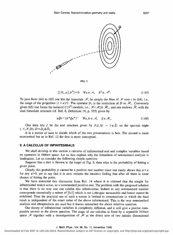
Suppose that a dart is thrown to the target of Fig. 5; then what is the probability of hitting a given point.
Clearly this probability p cannot be a positive real number since one easily shows that p< E for any &O, yet to say that it is zero violates the intuitive feeling that after all there is some chance of hitting the point.
We have extracted this discussion from Ref. 14 where it is claimed that the sought for infinitesimal makes sense, as a nonstandard positive real. The problem with this proposed solution is that there is no way one can exhibit this infinitesimal. Indeed to any nonstandard number corresponds canonically a subset of [O,l] which is not Lebesgue measurable and hence cannot be exhibited. Thus the practical use of such a notion is limited to computations in which the final result is independent of the exact value of the above infinitesimal. This is the way nonstandard analysis and ultraproducts are used but it leaves untouched the above intuitive question.
Our theory of infinitesimal variables is completely different, and it will give a precise com- putable answer to the above question. The stage of our calculus is fixed by a separable Hilbert space ,F together with a decomposition of A? as the direct sum of two infinite dimensional
J. Math. Phys., Vol. 36, No. 11, November 1995 Downloaded 22 Feb 2007 to 129.132.239.8. Redistribution subject to AIP license or copyright, see http://jmp.aip.org/jmp/copyright.jsp

6208 Alain Connes: Noncommutative geometry and reality
subspaces. To encode this decomposition we let F be the linear operator in .% which acts as the identity on the first subspace and as minus identity (Ft= - 5) on the second. One has by con- struction
F=F*, F*=l. (2.1)
At this point the stage is empty, it contains no information since any two couples (%,F) are unitarily isomorphic. This follows because all separable infinite dimensional Hilbert spaces are pairwise isomorphic.
We shall now write the beginning of a long dictionary showing how the classical notions appear in our “quantum mechanical” or spectral stage:
Classical
Complex variable Real variable Infinitesimal Infinitesimal of order LY
Differential of real or complex variable
Integral of infinitesimal of order 1
Quantum
Operator in 2% Self-adjoint operator in ,E Compact operator in .9? Compact operator in 28’ whose characteristic values pa satisfy pn=&Qz-a), n--+00 dif=[F,f]=Ff-fF
Dixmier trace
Let us explain in detail this part of the dictionary. The first two entries are just the basic notions of quantum mechanics. The range of a complex variable corresponds to the spectrum Sp(T) of an operator T in 567. The holomorphic functional calculus for operators in 28 gives meaning to f(T) for any holomorphic function f defined on the spectrum Sp T and the spectral mapping theorem of von Neumann controls the spectrum off(T). The holomorphic functions f are the only ones to act in that generality and this reflects the basic difference between complex analysis and real analysis where arbitrary bore1 functions act. Indeed when the operator T is self-adjoint f(T) now makes sense for any bore1 function f on the line. At this point let us note that a usual real random variable X on a probability space (fI,P) can in a trivial way be considered as a self-adjoint operator in Hilbert space. One lets .%=L2(fl,P) and T be the multiplication operator by X,
(2.2)
The spectral measure of T then gives back the probability P and no information has been lost in trading the probabilistic description for its Hilbert space counterpart. Of course all measure classes and multiplicity functions appear for self-adjoint operators T in 29.
Let us now describe the third entry of the dictionary. We wish to find nonzero “infinitesimal variables,” i.e., operators T in Hilbert space such that
IlTlj<~ t/e>O. (2.3)
Here the norm \lTll is the operator norm, Sup{llT& lIdI= 1). If we take (3) literally we of course get Il~jl=O and T=O. But we can slightly weaken it as follows:
For any e>O there exists a finite dimensional subspace EC% such that IITIE’II < E. (2.4)
Here we let El be the orthogonal complement of E,
J. Math. Phys., Vol. 36, No. 11, November 1995
Downloaded 22 Feb 2007 to 129.132.239.8. Redistribution subject to AIP license or copyright, see http://jmp.aip.org/jmp/copyright.jsp

Alain Connes: Noncommutative geometry and reality 6209
FIG. 6.
E’={~E%, (.$q+=O V~EE}, (2.5)
which is a subspace ofjnite codimension in %‘. The symbol TIE’ means the restriction of T to EL,
TIE’:E’+.%. (2.6)
The operators in .3? satisfying condition (4) are the compact operators, i.e., are characterized by the compactness for the norm topology of the image of the unit ball in 33. An operator T is compact iff its absolute value ITI = m is compact and this holds iff the spectrum of ITI is a sequence (PJ, P, -0. The eigenvalues /L,, of ITI arranged in decreasing order (cf. Fig. 6) are called the characteristic values of T and one has
pPI(T)=Inf{llT-RII; R operator of rank<n}.
Thus p,,(T) is I\Tll, the norm of T and
(2.7)
,uu,(T)=Inf{llT/E’Il; dim E=n}. (2.8)
The compact operators form a two sided ideal in the algebra S(.%) of bounded operators in .%’ and this ideal .3? is the largest two sided ideal of Z(L%). Thus the sum of two infinitesimal variables is still infinitesimal as well as the products infinitesimalxbounded and bounded Xinfinitesimal. These algebraic facts are easy to check using (7).
We are now ready to discuss the 4th entry of the dictionary. The size of the infinitesimal T E.,Z’ is governed by the rate of decay of the sequence /.L~( T) as n-+m. In particular for each positive real number LY the condition,
pn(T)=O(nMa) when nv+m (2.9)
(i.e., there exists C<a such that ~~(,(T)<cn -a Vn 3 1) defines the infinitesimals of order a. They form again a two sided ideal as is easily checked using (7) and moreover
Tj of order aj*T, T2 of order (Y, + CY*. (2.10)
Thus again the intuitive properties (except for commutativity) of infinitesimals are fulfilled. (For a< 1 the corresponding ideal is a normed ideal which is obtained by real interpolation between the ideal 2.’ of trace class operators and the ideal %’ (cf. Ref. 8)). At this point, since the size of infinitesimals is governed by a sequence Pi, ,u~ +O, it could seem that we may dispense with operators altogether and replace the above discussion of the ideal % in Z(%) by that of the ideal C,(N) in the algebra r”(N) of bounded sequences. A variable would just be a bounded sequence and an infinitesimal a sequence ,u,, , ~~40, n+m. However we would immediately lose the existence of variables with continuous range since all elements of p(N) have pure point spectrum and counting spectral measure, while operators in .% can have arbitrary spectral measures.
In fact the next entry of the dictionary exploits in a crucial way the lack of commutativity of x(.3). We replace the differential df of a real or complex variable, usually given by the differ- ential geometric expression,
J. Math. Phys., Vol. 36, No. 11, November 1995 Downloaded 22 Feb 2007 to 129.132.239.8. Redistribution subject to AIP license or copyright, see http://jmp.aip.org/jmp/copyright.jsp
6210 Alain Connes: Noncommutative geometry and reality
df=S-$dx’ (2.11)
by the operator theoretic expression
df =[F,fl. (2.12)
The transition from (11) to (12) is entirely similar to the transition from the Poisson bracket cf,g} of two observables of classical mechanics to the commutator u,g] =fg-gf of quantum mechanical observables. In order to be able to do calculations of a differential geometric nature we just need an algebra ,& of real or complex variables, i.e., an (involutive) algebra &3 of operators in 3% and we need to assume that these variables are differentiable inasmuch as
[Ff]E.% Vf EA. (2.13)
The equality F*= 1 shows that d(df) =0 for any f, i.e., that [F,f] anticommutes with F. The dimension of the differential space one is dealing with is governed by the degree of regularity of the variables f E&S, i.e., by the size of their differentials df. In dimension p one has
df of order j for any fE&. (2.14)
We shall come to concrete examples involving Julia sets and Hausdorff dimension very soon but we just briefly mention that it is Eq. (12) together with elementary manipulations on the functional
Trace(pdf’...df”) n odd, n>p, (2.15)
which led to cyclic cohomology. It allowed us in particular to transpose the ideas of differential topology to our framework and prove purely topological results using the above calculus and exploiting the integrality properties of the cocycle (15).
However, if the dictionary would stop here we would still miss an essential feature of the ordinary differential calculus, namely, the possibility of neglecting all infinitesimals of order >l when doing a computation. In our case the infinitesimals of order Y-1 form a two sided ideal whose elements satisfy
,dT)=o ; , 0 where the little o has the usual meaning, i.e., here that n p,(T) -+O when n -+a. But if we use the trace, as in (15), to integrate our infinitesimals then two things go wrong:
(a) The infinitesimals of order 1 are not in the domain of the trace. (b) The trace of higher order infinitesimals does not vanish.
Let us discuss these two points more carefully. The natural domain of the trace is the two sided ideal B” of truce class operators, i.e., of compact operators T such that,
30
q /-4W~. (2.17)
The trace of an operator T E B”(S?) is given by the sum
J. Math. Phys., Vol. 36, No. 11, November 1995
Downloaded 22 Feb 2007 to 129.132.239.8. Redistribution subject to AIP license or copyright, see http://jmp.aip.org/jmp/copyright.jsp

Alain Connes: Noncommutative geometry and reality 6211
Trace(T)=C (T&,&), (2.18)
which is independent of the choice of the orthogonal basis (L) of SZ. Moreover it is equal to the sum of the eigenvalues of T and in particular when T is positive one has
Trace(T)=% pn(T) for TZ=O. (2.19)
Now when T is an infinitesimal of order 1, say T20, the only control that we have on the size of P,,(T) is
~,,tT)=o ; ii
and this does not suffice to ensure the finiteness of (19). This shows the nature of the problem a) and similarly for b) since the trace does not vanish on the smallest of all ideals in 5?(S$l, namely, the ideal .R of finite rank operators.
Both of these problems are resolved by the Dixmier trace which is the 6th entry of our dictionary. For an infinitesimal of order 1 the sum (19) is at most logarithmically divergent since using (20) one has
N
T tdT)~C log N. (2.2 1)
We shall now describe in some detail the remarkable additivity property of the coefficient of the logarithmic divergency and more precisely of the cut off sums,
& /-4T), i-0. (2.22)
In fact it is convenient to use any positive real number X as a cut off instead of just the integers N and there is a nice formula which achieves this. Let for T a compact operator
a~(T)=Inf{llxlll+Allyllm; x+y=T), (2.23)
where 11 (II is the 55’ norm, IbII,=Tracelxl and )I II m is the operator norm. Then at integer values of A one has
N-l
UN(T)= 7 ,4T). (2.24)
Moreover one can show that the function X+ax(T) is the affine interpolation between its values on NCR: (Fig. 7).
The partial sums a, have the following properties:
q,(T,+T2)~ax(T,)+ah(T,) VT,,TZ~.%-, XER~, (2.25)
~h,+h2(T1+T2)~~.h,(T1)+~.h2(T2) if TI,T~~O, (2.26)
and for any X, , X2 E R*, .
J. Math. Phys., Vol. 36, No. 11, November 1995 Downloaded 22 Feb 2007 to 129.132.239.8. Redistribution subject to AIP license or copyright, see http://jmp.aip.org/jmp/copyright.jsp

6212 Alain Connes: Noncommutative geometry and reality
FIG. 7.
The remarkable additivity property of the coefficient of the logarithmic divergence (22) is expressed as follows, where T, , T, are positive and satisfy (21)
where for any T>O one lets
(2.27)
(2.28)
be the Cesaro average of oJlog u in the multiplicative group RT of cut off scales. The inequality (21) shows that the value of q,(T) is bounded independently of XE Wf ,
OGs-,(T)GC for TSO satisfying (21) and as X +a the functionals rA become more and more linear by the inequality (27).
The Dixmier trace Tr, is defined as any limit point of the functionals TV
Tr,= lim r,, , X-v=
(2.29)
where the choice of the limit point is encoded by the index W. In practice this choice is not important because in all relevant examples the following mea-
surability condition is satisfied
Q(T) is convergent when X-co. (2.30)
The Dixmier trace Tr, is extended by linearity to the two sided ideal of infinitesimals of order 1 and enjoys the following properties, which cure the defects (a) and (b) of the ordinary trace,
LY) Tr, is a linear positive trace with domain the two sided ideal of infinitesimals of order 1, thus
J. Math. Phys., Vol. 36, No. 11, November 1995
Downloaded 22 Feb 2007 to 129.132.239.8. Redistribution subject to AIP license or copyright, see http://jmp.aip.org/jmp/copyright.jsp
Alain Connes: Noncommutative geometry and reality
Tr,(X,T,+X2T2)=X, Tr,(T,)+X, Tr,(T,) \dXjEC,
Tr,(ST)=Tr,(TS), for any bounded S,
Tr,(T)>O, whenever T3 0.
/?) Tr,(T)=O h w enever the order of T is > 1, in fact,
1 Tr,(T)=O if p,(T)=0 ; . 0
6213
(2.31)
(2.32)
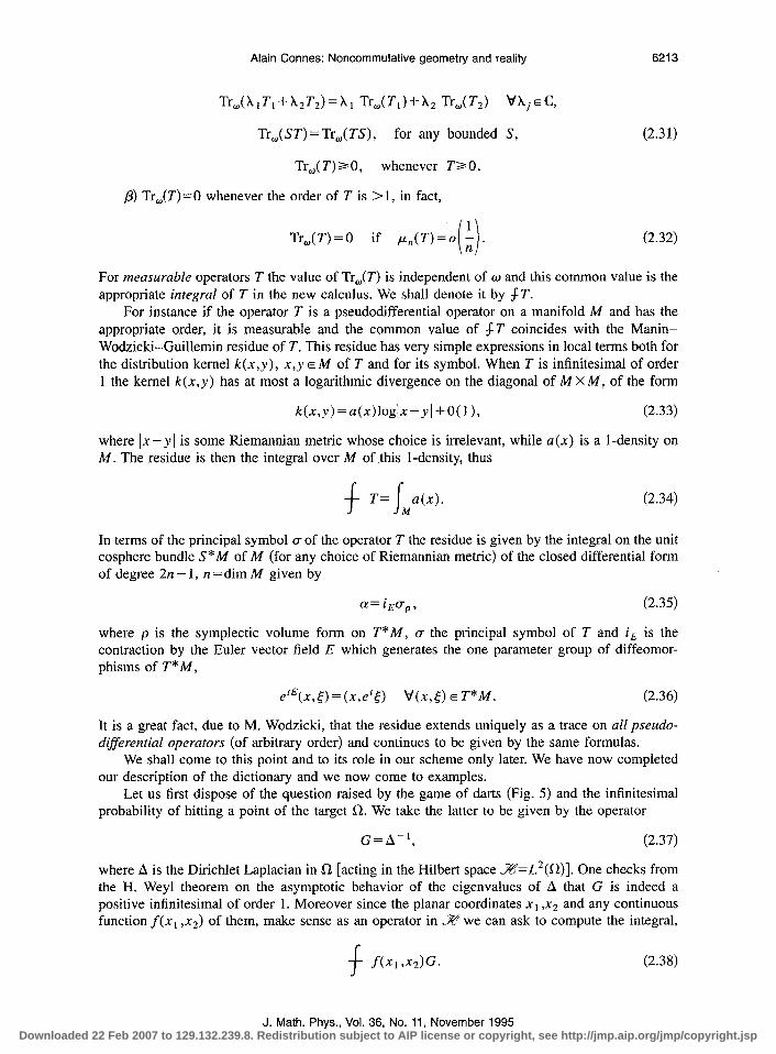
For measurable operators T the value of Tr,(T) is independent of w and this common value is the appropriate integral of T in the new calculus. We shall denote it by ST.
For instance if the operator T is a pseudodifferential operator on a manifold M and has the appropriate order, it is measurable and the common value of $‘T coincides with the Manin- Wodzicki-Guillemin residue of T. This residue has very simple expressions in local terms both for the distribution kernel k(x,y), x,y E M of T and for its symbol. When T is infinitesimal of order 1 the kernel k(x,y) has at most a logarithmic divergence on the diagonal of MXM, of the form
~tx,p)=a(x)loglx-yI+0(1), (2.33)
where Ix-y] is some Riemannian metric whose choice is irrelevant, while a(x) is a l-density on M. The residue is then the integral over M of this l-density, thus
4x1. (2.34)
In terms of the principal symbol u of the operator T the residue is given by the integral on the unit cosphere bundle S*M of M (for any choice of Riemannian metric) of the closed differential form of degree 2n - 1, n =dim M given by
cu=ipp, (2.35)
where p is the symplectic volume form on T*M, CT the principal symbol of T and i, is the contraction by the Euler vector field E which generates the one parameter group of diffeomor- phisms of T*M,
ef”tx,5) = (x2.9 ‘#(x,5) E T”M. (2.36)
It is a great fact, due to M. Wodzicki, that the residue extends uniquely as a trace on all pseudo- differential operators (of arbitrary order) and continues to be given by the same formulas.
We shall come to this point and to its role in our scheme only later. We have now completed our description of the dictionary and we now come to examples.
Let us first dispose of the question raised by the game of darts (Fig. 5) and the infinitesimal probability of hitting a point of the target Sz. We take the latter to be given by the operator
G=A-,, (2.37)
where A is the Dirichlet Laplacian in R [acting in the Hilbert space %=~~(n)]. One checks from the H. Weyl theorem on the asymptotic behavior of the eigenvalues of A that G is indeed a positive infinitesimal of order 1. Moreover since the planar coordinates x, ,x2 and any continuous function f(x, ,x2) of them, make sense as an operator in % we can ask to compute the integral,
f ftx, ,x2&. (2.38)
J. Math. Phys., Vol. 36, No. 11, November 1995 Downloaded 22 Feb 2007 to 129.132.239.8. Redistribution subject to AIP license or copyright, see http://jmp.aip.org/jmp/copyright.jsp

6214 Alain Connes: Noncommutative geometry and reality
One can show that fG is indeed measurable and compute the value of (38), it gives Snf(x, ,-Qdx,~dx2, i.e., the ordinary Lebesque integral off with respect to the area measure on i-l.
In this answer to our original question on the game of darts we did not use the 5th entry of the dictionary, i.e., differentiation. To see how this works and allows operations not doable in distri- bution theory we shall discuss our calculus in the case of functions of a single real variable, i.e., the space we are discussing is X= W.
There is (up to unitary equivalence and multiplicity) a unique way to quantize the calculus on R in a translation and scale invariant manner. It is given by the representation of functions f on W as multiplication operators in L2(W), while the operator F in %=L*(R) is the Hilbert transform,
t..fS)ts)=fts)5ts) QEL2(W, SER, (Ft)(t)=$j- sds.
One can give an equivalent description for S’=P,(R), with %‘=L2(S’) while F is again the Hilbert transform,
Fe,=sign(n)e,, e,(@=exp in0 VBES’ (sign O=l). (2.40)
Using (39) one readily computes the kernel k(s,t) given by the differential [F,f], it is given, up to the constant l/m’, by
k(s t) = f(s) -f(t) 7
s-t (2.41)
The first virtue of the new calculus is that df continues to make sense, as an operator in L2(S’) for an arbitrary measurable f E L”(S’). This of course would also hold if we define df using distribution theory but the essential difference is the following. A distribution is defined as an element of the topological dual of the locally convex vector space of smooth functions, here C”(S’). Thus only the latter linear structure on C”(S’) is used, not the algebra structure of C”(S’). It is consequently not surprising that distributions are incompatible with pointwise prod- uct or absolute value. Thus more precisely while, with f nondifferentiable, df makes sense as a distribution, we cannot make any sense of ldfl or powers ldflp as distributions on S’. Let us give a concrete example where one would like to use such an expression for nondifferentiable f. Let c be a complex number and let J be the Julia set given by the complex dynamical system z-+z’+c= q(z). More specifically J is here the boundary of the set B={z EC; supntN I@(z)l cm}. For small values of c as the one chosen in Fig. 8, the Julia set J is a Jordan curve and B is the bounded component of its complement. Now the Riemann mapping theorem provides us with a conformal equivalence 2 of the unit disk, D = {z E C;lzl< 1) with the inside of B, and by a result of Caratheodory, the conformal mapping Z extends continuously on the boundary S’ of D to a homeomorphism, which we still denote by Z, from S’ to J. By a known result of D. Sullivan, the Hausdorff dimension p of the Julia set is strictly bigger than 1, 1 <p<2 and is close to 2 for instance, in the example of Fig. 8. This shows that the function Z is nowhere of bounded variation on S’ and forbids a distribution interpretation of the naive expression:
I ftz>ldZl” vf~ C(J), (2.42)
that would be the natural candidate for the Hausdorff measure on J. It turns out that the above expression, i.e., $f(Z) I &ZIP makes sense in the quantized calculus
and that it does give the Hausdorff measure on the Julia set J
J. Math. Phys., Vol. 36, No. 11, November 1995
Downloaded 22 Feb 2007 to 129.132.239.8. Redistribution subject to AIP license or copyright, see http://jmp.aip.org/jmp/copyright.jsp

Alain Connes: Noncommutative geometry and reality 6215
FIG. 8.
f ftZ)l~Zi’=~~Jfd~p. The first essential fact is that as BZ = [F,Z] is now an operator in Hilbert space one can, irre- spective of the regularity of Z, talk about I BZI, it is the absolute value IT[=(T*T)~‘~ of the operator T= [ F,Z]. This gives meaning to any function ~(Ic#z~) where h is a bounded measurable function on the spectrum of ldzl and in particular to [aZIP. The next essential step is to give meaning to the integral of f(Z) I &ZIP. The latter expression is an operator in L2(S’) and we use a result of hard analysis due to V. V. Peller, together with the homogeneity properties of the Julia set to show that the operator f( Z) I BzlP belongs to the domain of definition of the Dixmier trace Tr, , i.e., is an infinitesimal of order 1. Moreover, if one works modulo infinitesimals of order >l the rules of the usual differential calculus such as
turn out to be valid and show that the measure
f-‘Jk,,(ftZ) 1 dZIp) vf E (3.0 (2.45)
has the right conformal weight and is a nonzero multiple of the Hausdorff measure. The corre- sponding constant X governs the asymptotic expansion in n EN for the distance, in the sup norm on S’, between the function Z and restrictions to S’ of rational functions with at most n poles outside the unit disk.
For smooth functions on S’ there is a feature which is specific to dimension one and will not occur for higher dimensional manifolds, that df = [F,f] for f smooth is not only of order 1 =(dim S’)-’ but is in fact a trace class operator. Moreover,
Trace(PBf’)= fS,p df’ Vp,f' E C”(S’). (2.46)
J. Math. Phys., Vol. 36, No. 11, November 1995 Downloaded 22 Feb 2007 to 129.132.239.8. Redistribution subject to AIP license or copyright, see http://jmp.aip.org/jmp/copyright.jsp

6216 Alain Connes: Noncommutative geometry and reality
In fact the size of df = [ F,fl for f smooth can be as small as to belong to the smallest ideal A of finite rank operators and a classical result of Kronecker reads as follows,‘5
P(s) dffEj;R*f(s)=Q0 is a rational fraction. (2.47)
On the other extreme side of regularity, classical results of analysis due to Douglas, Fefferman, and Sarason” give
dfE.SY@f is VMO, (2.48)
i.e., f has vanishing mean oscillation. The quantized calculus applies in a similar manner to the projective space P,(K) over any
local field K (i.e., any nondiscrete locally compact field, commutative or not). The obtained calculus is invariant under the group SL(2,K) of projective transformations. The special cases of K=C and K=H (the field of quatemions) will be covered and generalized by our next example of oriented even dimensional conformal compact manifolds.
Thus let M2n be such a manifold, of dimension 2n. The * operation on differential forms of degree n = $ dim M only depends upon the oriented
conformal structure of M. We let .?Z be the Hilbert space of these square integrable forms,
L~+~=L~(M,A~T*) (2.49)
with the canonical inner product,
(WI@2>' I
qA*cd2. M
The algebra of functions on M acts by multiplication operators in x,
(fE)(x)=f(x)Mx), ~~EL~(M,A"T*), XEM (2.5 1)
and it just remains to describe the operator F, F= F*, F2 = 1, in % We just let
F=2P- 1, P= orthogonal projection on exact forms. (2.52)
A form is exact iff it belongs to the image of the exterior differentiation d. We shall now describe two applications of this quantized calculus for conformal manifolds.
The simplest instance of the above construction is when n = 1, i.e., when M is a Riemann surface: a compact complex curve. The complex structure on M is equivalent to its oriented conformal structure. For any smooth function f on M the commutator df = [ F,f] is an infinitesimal of order i=(dim M)-’ and one obtains
f (2.53)
Let then X be a smooth map from M to the target space RN endowed with a Riemannian metric gpvdxp dx”. The components XP of the map X are functions on M and it immediately follows from (53) that
f g,,(x)dX’L dX’=; Mgpv dXp//*dX’. I
(2.54)
J. Math. Phys., Vol. 36, No. 11, November 1995
Downloaded 22 Feb 2007 to 129.132.239.8. Redistribution subject to AIP license or copyright, see http://jmp.aip.org/jmp/copyright.jsp

Alain Connes: Noncommutative geometry and reality 6217
Now the right hand side is Polyakov’s form of the Nambu action which is the starting point of string theory.
Let us now consider the case of 4-manifolds M4. Then the right hand side written as J,+,g,,,(dX’*,dX”) is not conformally invariant. We shall see that the left hand side continues to make sense thanks to the quantized calculus and gives a much more subtle, and conformally invariant analog of the Polyakov action in the 4-dimensional case. Indeed the quantized calculus on M4 only depends upon its conformal structure so the value of $g,,(X)BXp BX” is necessarily conformal. It does make good sense thanks to the result of M. Wodzicki, mentioned above, which extends the domain of f to all pseudodifferential operators.
After a lengthy calculation one obtains
f g,,(X)dX’* dX’=( 167r2)-’ g,,(X){fr(dX~,dX”)-A(dXp,dXV)+(VdX’L,VdXV)
- $(AXF)(AXY)}du, (2.55)
where to write down the right hand side one has used a Riemannian structure on M compatible with the given conformal structure. In the right hand side the scalar curvature r, the Laplacian A and the Levi-Civita connection V all refer to this additional Riemannian metric, but the result is independent of its choice.
We shall come back to (55) later in our discussion of metrics and of the Einstein-Hilbert action. When the g,, are constant independent of X the above quadratic action is given by the Paneitz operator on M. This operator has order 4 and plays the role of the Laplacian in 4-dimensional conformal geometry (cf. Ref. 16). The conformal anomaly for its determinant has been computed by T. Branson.”
We also note that a similar discussion relates the p-adic string action’* with the quantized calculus over Pi (K) with K the field Qp of p-adic numbers. This situation being O-dimensional the $ integral is replaced by the trace.
Let us now describe a second application of our construction, it provides local formulae for Pontrjagin classes of topological manifolds.” By the deep results of S. Novikov and D. Sullivan20*21 any compact topological manifold M”, n #4 admits a quasiconforma/ structure, i.e., a collection of local charts whose overlap homeomorphisms cp are quasiconfotmal, i.e., satisfy, for some KC?
H,(x)=liy+v minlqo(x)-cp(y)l;lX-yl=r SK, ~.XE Domain cp. (2.56)
It turns out that this quality of a manifold M, being quasiconformal, is exactly what is needed to quantize the calculus on M. [It is of course much less than smoothness since many topological manifolds cannot be smoothed (cf. Ref. 11) for instance).] To see this we shall explain how the above quantized calculus on a conformal manifold M is modified by a change of the conformal structure within the same quasiconformal class. For simplicity we begin by the 2-dimensional case. Let us note that since we are in the even case there is a natural Z/2 grading y of the Hilbert space (49) of middle dimensional forms, given by
yo= i*w. (2.57)
Now, in the a-dimensional case, a change of the conformal (or complex) structure of M is provided exactly by a Beltrami differential ,u, i.e., with a local complex coordinate Z,
,u(z,f)dildz, j,u(z,Z)I<1. (2.58)
J. Math. Phys., Vol. 36, No. 11, November 1995 Downloaded 22 Feb 2007 to 129.132.239.8. Redistribution subject to AIP license or copyright, see http://jmp.aip.org/jmp/copyright.jsp

6218 Alain Connes: Noncommutative geometry and reality
To obtain the new conformal structure at z EM one uses, in order to define angles at z, the map
XE T,(M)-(X,dz+p(z,Z)dZ) EC
instead of the map X+(X,dz). The new conformal structure is in the same quasiconformal class as the old one iff ,U is
measurable and satisfies
IMlm< 19 (2.59)
where 11 Ilm is the L” norm of p(z,Z), a meaningful notion independently of local coordinates. Next recall that our Hilbert space 3 is in this case the space of square integrable l-forms,
%‘=L2(M,A1T*). The Z/2 grading y gives the decomposition of 2 in forms of type (1,0) on which y= 1 and of type (0,l) on which y= - 1.
To a Beltrami differential p corresponds an operator in $Y, namely, the endomorphism 6 of the bundle A’T* given by the matrix,
0 jqz,Z) =
,G(z,i!)dzldZ
&z,i)dZldz I 0 . (2.60)
Moreover one obtains in this manner exactly all operators in Z which satisfy
#LIE.&‘, F=b”, by= - YL Ilbll< 13 (2.61)
where -4” is the commutant of the algebra ,g of functions on M,
,/A’={TEZ(.%); Ta=aT VUE&}. (2.62)
The quantized calculus on M obtained from the new conformal structure is obtained from the old one by a beautiful general formula. One leaves the Hilbert space .% and the representation of ~8 in X untouched. One only modifies F by a Moebius transformation, the new F is given by
F’=(crF+p)(PF+a)-‘, (2.63)
where the operators a,/3 are CX=(~-~~)-“*, p = i;( 1 - /I*)-l’*. The key point then is the fol- lowing formula which relates the differentials in the old and new conformal structures,
[F’,f]=Y[F,f]Y*, Y*=(/?F+a)-‘, (2.64)
which shows that the order of the infinitesimal [F,f] is independent of the change of conformal structure (cf. Ref. 8).
All these facts extend to higher dimension and using them for the sphere S2” one shows” that the construction (49)-(52) of the quantized calculus on a conformal manifold applies to any bounded measurable conformal structure on a quasiconformal manifold. Using cyclic cohomology and Alexander Spanier cohomology instead of the Chem-Weil curvature calculations one obtains the desired formula for the topological Pontrjagin classes.”
III. GAUGE THEORY AND THE STANDARD MODEL
Let us now return to our spectrally defined spaces of Sec. I and explain how to use the above calculus of infinitesimals. Given a spectral triple (JA,.%‘,D) we let F be the sign of D,
F=Sign D=DIDl-I, (3.1)
J. Math. Phys., Vol. 36, No. 11, November 1995
Downloaded 22 Feb 2007 to 129.132.239.8. Redistribution subject to AIP license or copyright, see http://jmp.aip.org/jmp/copyright.jsp

Alain Connes: Noncommutative geometry and reality 6219
where by convention sign(O) = 1. Since D is self-adjoint this makes good sense and moreover one has
F=F”, F*= 1. (3.2)
Thus a spectral triple gives in particular an involutive algebra represented in the Hilbert space X and an operator F in .X satisfying (2) which is the stage of the quantized calculus. Moreover the basic conditions a) fl) of Definition 1 show that,
[F,U]E.% V’aEd& (3.3)
Let us now explain the meaning of the remaining data, namely,
IDI=(D2)“2 (3.4)
which appears in the spectral triple. In order to do geometry we not only need our algebra of coordinates ~6 acting in the stage
(X,F) of the quantized calculus. We also need an infinitesimal unit of length 6= “ds” to which the differentials da = [F,a] of elements of ~6 can be compared. Since infinitesimals are compact operators in Z’ we need a positive compact operator in 2. Its relation with IDI is the following:
tf=IDI-‘. (3.5)
(The value of / on the finite dimensional kernel of IDI is irrelevant.) Giving the operator D is the same thing as giving the pair of operators F and 6, and note that
since F and IDI commute one has
d/=[F,/]=O. (3.6)
For elements of . -A which are in the domain of the derivation S (formula 27 of Sec. I) the two operators [F,u]JDJ and [IDI, ] a are bounded which means that the size of da is controlled by that of / and that the size of [/,a] is of the order of L*.
Due to noncommutativity the relevant choice for the ratio of Ba with / is the combination [D,u] which we already used in Sec. I to measure distances in the spectrum of .A by
d(cp,~)=Sup{lcp(a)-~ta)l; a~,&:, il[D~alll~l) (3.7)
for any pair cp, (c, of states on . ;Z (commutative or not). The quantized calculus now gives us the general analog of integration with respect to the
Riemannian volume element. In a spectral triple (,A,X,D) of dimension p>O the unit of length /=IDl-’ is an infinitesimal of order l/p and the analog of the volume integral is
f f/P VfE"4. (3.8)
In the usual Riemannian case (1.31) this gives indeed the right answer (with a numerical coeffi- cient in front). In general it gives a positive truce on -4, i.e., a functional r such that
T(f *f)ao Vf E .A, T(ab)= T(ba) Va,b E./S. (3.9)
We shall now proceed in two steps to develop geometric concepts for spectral triples. The first step will develop the analog of the matter Lagrangian of Q.E.D. The second step will go towards the gravitational Lagrangian by giving a general local formula for the global index information con- tained in the operator D.
J. Math. Phys., Vol. 36, No. 11, November 1995 Downloaded 22 Feb 2007 to 129.132.239.8. Redistribution subject to AIP license or copyright, see http://jmp.aip.org/jmp/copyright.jsp

6220 Alain Connes: Noncommutative geometry and reality
Let us thus begin by gauge theory. Since J& is an involutive algebra it has a well defined unitary group,
%={u EJ& uzl*=u*u= l}. (3. IO)
For instance when ,& is the algebra of (complex valued) functions on a manifold M one has
%=Map(M,U( l)), (3.11)
while when .& is the algebra of N X N matrix valued function on M one has
%=Map(M,U(N)), (3.12)
the group of all maps (with a given degree of smoothness) from the manifold M to the Lie group u(N).
Since the algebra J$? acts in X, this provides a natural representation of ,?z% in 2 given by
(u,.g-tu~ VUE’& gTE.sY. (3.13)
The action functional given by
5-(5B5) (3.14)
is not invariant under the gauge transformation (13) since the operator D does not commute with the algebra -I&, thus
uDu”#D in general, for u E “Z. (3.15)
To restore the gauge invariance one introduces vector potentials and an affine action of the group ?d on the space of vector potentials as follows. A vector potential A is simply an arbitrary self-adjoint (bounded) operator in .% of the form,
A=ZUi[D,bi], ai,biE~. (3.16)
Thus A =A * and the space of vector potentials is by construction a linear space of self-adjoint operators in X. It is the self-adjoint part of the linear space of all operators of the form (16). One checks that the latter space s2 is a bimodule over .A;, i.e., that
YECl, a;bE&*aYbeR (3.17)
as follows from the equality [D,bJb= [D,bib] - bi[D,b]. The gauge transformations on vector potentials are given by
y,(A)=u[D,u*]+uAu* VA=A*, Aef2, u E ,+?A (3.18)
and it follows from (17) that y,(A) is a vector potential, i.e., a self-adjoint element of a. Moreover the following action functional is now gauge invariant,
&A-+(&(D+A)5), (3.19)
since one has D+ y,(A)=u(D+A)u* Vu E ‘%. We now need to write down the self-interaction of the vector potential A and the first question
is to find the field strength or curvature 0. Given A=Ea,[D,b,] we postulate
O=C[D,ai][D,bi]+A*. (3.20)
J. Math. Phys., Vol. 36, No. 11, November 1995
Downloaded 22 Feb 2007 to 129.132.239.8. Redistribution subject to AIP license or copyright, see http://jmp.aip.org/jmp/copyright.jsp

Alain Connes: Noncommutative geometry and reality 6221
We shall first ignore the problem that A can have several inequivalent representations as A =Cai[D,bi] creating an ambiguity in the formula (20). Thus we shall compute what is the curvature 19 for the gauge transformed vector potential y,(A),
yu(A)=u[D,u*]+CuUi([D,biu*]-bi[o,u*]), (3.21)
where we wrote [D,bj]u*=[D,biu*]-bi[D,u*]. Thus the new curvature 8’ is given, using (20), by
8’=[D,u][D,u*]+C[D,uUi][D,biu*]-Z[D,uaibi][D,u*]+(y,(A))‘. (3.22)
Now y,(A)2=(u[D,u*]+uAu*)2=(u[D,u*])2+u[D,u*]uAu*+uA[D,u*]+~A2~*. A straightforward computation shows that
e’=ueu*. (3.23)
Thus curvature transforms in a covariant way and we define the self-interaction of the vector potential A by
i.e., by the integration [formula (S)] of the square of the curvature. It is gauge invariant by construction. Let us now take care of the ambiguity in the definition of 8. First we only deal with self-adjoint elements A of R and in writing A = Ca,[D,b,] we can always assume the following:
Caib;=O, Cai~bi=~b”~a” (in .&@%A). (3.25)
[ReplaceCa,@bi byCai@bi-(EUibi)@ 1 forthefirstconditionandby ~C(ai @ bi + b* @ at? for the second.]
Under these conditions (25) the curvature B satisfies 8= 8”” which shows that (24) is positive. The curvature 8 belongs to the self-adjoint part of the ,,B-bimodule,
~*={ZAiBi; Ai,BiEn}. (3.26)
Note that,
!Fl*={Cai[D,bi][D,ci]; ai ,bi ,CiE ~~}. (3.27)
The ambiguity in 0 is given exactly by the self-adjoint part of the following subspace of Cl*,
.T={C[D,Ui][D,bi]; ai,bi~h3, ZUi[D,bi]=O}. (3.28)
The simplest way to remove this ambiguity is to replace t9 in (24) by its orthogonal projection P( 0) on the orthogonal .p of .7in Cl*, where we endow a2 with the positive inner product,
(X,Y)= f XY”P. (3.29)
As .7is a subbimodule of a*, i.e., satisfies
ajbE,F VjEY, a,bE& (3.30)
one gets that P(aXb)=aP(X)b Va,b E,/%, XE a*, which ensures the gauge invariance of the unambiguous functional
f P( ej2t’p. (3.3 1)
J. Math. Phys., Vol. 36, No. 11, November 1995 Downloaded 22 Feb 2007 to 129.132.239.8. Redistribution subject to AIP license or copyright, see http://jmp.aip.org/jmp/copyright.jsp

6222 Alain Connes: Noncommutative geometry and reality
One obtains an equivalent theory if one keeps the ambiguity and introduces the auxiliary field given by the orthogonal decomposition
a=e-P(e). (3.32)
Clearly a can be any self-adjoint element of 3, and the full action (24) now reads,
(As)+ f p( e)*tip+ f a2Lp= f 8*/p. (3.33)
The equations of motion for this action sets the a to the value a = 0, and thus it is a matter of taste whether
The full
we keep the a’s or not. The action of the gauge group % on these auxiliary fields is
yu(a)=uau* Vu Ez a=a*, u E 2!4. (3.34)
Q.E.D. action can now be written,
f 82/p+(&(D+A)t). (3.35)
In the simplest example, of the Dirac spectral triple on a spin Riemannian manifold M the action (35) is the (Euclidean version of the) action of massless quantum electrodynamics. In the next simplest example of the algebra of N X N matrices of functions on M acting in the Hilbert space L2(M,S@CN) while D =BEA@ 1, the action (35) is the Yang-Mills action for a massless fermion in the fundamental representation of the gauge group U(N).
The first remarkable fact about the action (35) is that if we compute it for the product of a Riemannian space M by the finite geometry Y of example of Sec. I (with p a nontrivial matrix) we obtain a Lagrangian with 5 terms which reproduce the Glashow-Weinberg-Salam model for leptons, with its Higgs sector with quartic symmetry breaking self-interaction and the parity violating Yukawa coupling with fermions (cf. Ref. 8 for more detail). The computation is com- plicated but the underlying idea is simple.
The Higgs fields appear as the finite difference part of the vector potential. Indeed differen- tiation in the M X Y involves differentiation on each copy of M as well as the finite difference in the Y direction, so that a vector potential A decomposes as a sum of a component of differential type A”*‘) and a component of finite difference type A’07” which gives the Higgs fields.
Similarly the field strength or curvature 0 has 3 components of respective type (2,0), (1, l), and (0,2). They yield, respectively, the three terms JZo, ZoH, ZH of the GWS Lagrangian, where Zo is the Yang-Mills self-interaction, KoH the minimal coupling with the Higgs and ZH the quartic Higgs self-interaction.
The geometric picture that emerges is that of a space with two sides, with opposite orienta- tions, each point pL of one side having a corresponding point pR on the other, with distance of the order of the inverse of the mass scale of the theory, d(pL,pR)-l/p, where p is the largest eigenvalue of the matrix.
But the true standard model also involves quarks, with a nonzero mass for the up quarks, as well as the strong forces.
We described in Ref. 22 and Ref. 8 how to modify the above simple picture in order to obtain the Lagrangian of the standard model, but there was still some artificial part in our construction, namely, the use of “bivector potentials” (cf. Ref. 8, p. 594) and of the “unimodularity condition” (cf. Ref. 8, p. 609). We shall explain here how these two problems are solved and how the symmetry is restored in the Poincare duality of Ref. 8.
At first sight the action functional (35) is similar to the supersymmetric pure Yang-Mills functional, but looking more closely there is a basic and crucial difference:
In (35) the fermions are in the fundamental representation (of the gauge group). As is well known this is not what happens in pure Yang-Mills supersymmetry where the fermions are Majorana spinors in the adjoint representation.
J. Math. Phys., Vol. 36, No. 11, November 199.5
Downloaded 22 Feb 2007 to 129.132.239.8. Redistribution subject to AIP license or copyright, see http://jmp.aip.org/jmp/copyright.jsp

Alain Connes: Noncommutative geometry and reality 6223
As we shall see now a real structure J on a spectral triple (.&.K,D) provides u,s with an analog of the adjoint representation for the unitary group 2 of J. Let us first recall the Definition 3 of Sec. I.
Definition 3: Let (. &X,0) be an even spectral triple. A real structure of mod 8 dimension 2k is an antilinear isometrq J in X such that:
CY) JD=DJ, J2=e, Jy=e’yJ. p) For any a E .,& the operators a and [D,a] commute with J,AJ”, where the table of signs for
e,d is gilten in Sec. I.
As in the theory of operator algebras, where J is Tomita’s involution, (cf. Ref. 8, V, Appendix B) it is convenient to use the following notation for the J-bimodule structure of .Z coming from J,
aeb=aJb*J*t Va,bE,& V.$E,%.
The commutation of a with Jb*J* for any a,b E J$ is then encoded in the equality
(3.36)
a(@) = (aE)b, (3.37)
which is a familiar rule for the standard representation of a von Neumann algebra (cf. Ref. 8). The natural adjoint action of the unitary group % of I 4 on the Hilbert space 2% is thus given
by the unitary operator
associated to any u E r’d.
~-)u~u*=uJuJ*~ V(EX (3.38)
If for instance the mod 8 dimension is such that J2= 1 then these unitaries preserve the real subspace {&Jt=t}. Now if we conjugate the operator D by this adjoint section of ?A on 2 we obtain, using cr) /I) of Definition 3,
(uJuJ*)D(uJuJ*)*=D+u[D,u*]+J(u[D,u*])J*. (3.39)
More generally we see that the gauge transformation (8) of vector potentials, y,(A) = u [D,u *] + uAu*, has the following compatibility with the adjoint action (38),
(uJuJ*)(D+A+JAJ*)(uJuJ*)*=D+ y,(A)+Jy,(A)J*
for any vector potential A and u E &.
(3.40)
Thus, we obtain an analog in our context of pure Yang-Mills action with Fermions in the adjoint representation as follows
@,5)-t f 02/p+(&(D+A+JAJ*)~). (3.41)
The action (41) is gauge invariant for the adjoint action (38) on fermions. As an example one can compute what it gives for the spectral triple where . & is the algebra of n X n matrices of functions on a Riemannian spin manifold M, acting on the left in the Hilbert space 5?=L*(M,S@M,(C)). One uses the left action of matrices on themselves. The operator D is B,+, @ 1. The real structure J comes from the adjoint operation T--+T” on matrices and the charge conjugation C on spinors. One obtains, using J to impose a Majorana condition on spinors, the pure Yang-Mills supersym- metric action with gauge group SU(n).
We shall now show that the standard model action is obtained by the action (41) on the product of the usual continuum of dimension 4 by a finite spectral triple.
We shall first describe in detail the finite real spectral triple which is needed to obtain the standard model action.
J. Math. Phys., Vol. 36, No. 11, November 1995 Downloaded 22 Feb 2007 to 129.132.239.8. Redistribution subject to AIP license or copyright, see http://jmp.aip.org/jmp/copyright.jsp

6224 Alain Connes: Noncommutative geometry and reality
SU(3) color
FIG. 9.
The algebra .& is .4=C@II@M,(C), i.e., it is the direct sum of complex numbers, quater- nions and 3X3 complex matrices. The involution on .R is given by (A,s,m)-&~,m*) where S is the usual conjugate of the quaternion 4.
Let ..Z=%@%, where i5 is the finite dimensional Hilbert space whose basis is labeled by all elementary fermions (Fig. 9). Here g denotes the complex conjugate Hilbert space (i.e., elements of E are of the form <, 5 E 8, with
x.$=(X()- VAEC. (3.44)
We now describe the action of & on Z, it is dictated by the natural apparent symmetries of Fig. 9 whose disposition is due to J. Ellis.* Both Z and % are globally invariant under this action, which is thus specified by its restrictions to 65 and to c!? which we now describe.
For % the action of (X,q,m) does not use m ems. For weak isospin singlets such as (ii) or eR it uses Only A which aCtS by
A( ;:j=(; ;;j, A(Q)=(&). (3.45)
For weak isospin doublets such as (1:) or (1:) one simply acts by the quatemion 4 = CT+ flj viewed as a 2X2 matrix, ck! P 4= 1 1 -p G acting on each doublet. (3.46)
For z the action of (A,q,m) does not use q and the action is by A on leptons and by m acting on the color indices for the quarks. It is clear that we thus have an action on .4 on 58.
Next the antilinear involution J is given by
J(&ij)=( q.g) V(E LF, +jE A?.
Finally the operator D in 5T? is given by
(3.47)
J. Math. Phys., Vol. 36, No. 11, November 1995
Downloaded 22 Feb 2007 to 129.132.239.8. Redistribution subject to AIP license or copyright, see http://jmp.aip.org/jmp/copyright.jsp
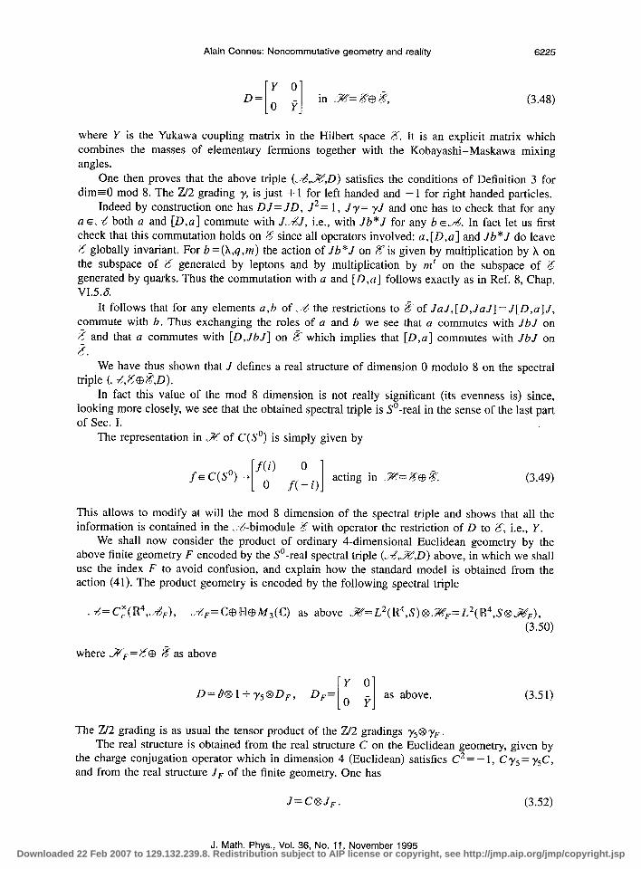
Alain Connes: Noncommutative geometry and reality 6225
Y 0 D=o r [ 1 in %= Z@@, (3.48)
where Y is the Yukawa coupling matrix in the Hilbert space 8. It is an explicit matrix which combines the masses of elementary fermions together with the Kobayashi-Maskawa mixing angles.
One then proves that the above triple (A’,X,D) satisfies the conditions of Definition 3 for dim=0 mod 8. The Z/2 grading y, is just + 1 for left handed and - 1 for right handed particles.
Indeed by construction one has DJ= JD, J2= 1, J y= yJ and one has to check that for any ~1 E, -?! both a and [D,a] commute with J&J, i.e., with Jb*J for any b E&L In fact let us first check that this commutation holds on % since all operators involved: a,[D,a] and Jb*J do leave % globally invariant. For b =(A,q,m) the action of Jb*J on Z is given by multiplication by A on the subspace of % generated by leptons and by multiplication by m’ on the subspace of % generated by quarks. Thus the commutation with a and [D,a ] follows exactly as in Ref. 8, Chap. VI.5.s.
It follows that for any elements a,b of ,& the restrictions to 8 of JaJ, [D,JuJ] = J[D,u] J, commute with b. Thus exchanging the roles of a and b we see that a commutes with JbJ on i? and that u commutes with [D,JbJ] on g which implies that [D,u] commutes with JbJ on 2.
We have thus shown that J defines a real structure of dimension 0 modulo 8 on the spectral triple (< -L,CCB%‘,D).
In fact this value of the mod 8 dimension is not really significant (its evenness is) since, looking more closely, we see that the obtained spectral triple is SO-real in the sense of the last part of Sec. I.
The representation in ..P of C(S’) is simply given by
f E C(SO)+ [‘Y’ f(“i)]
acting in B= Z% %+. (3.49)
This allows to modify at will the mod 8 dimension of the spectral triple and shows that all the information is contained in the .r%-bimodule Z with operator the restriction of D to 5, i.e., Y.
We shall now consider the product of ordinary 4-dimensional Euclidean geometry by the above finite geometry F encoded by the SO-real spectral triple (.A,B’,D) above, in which we shall use the index F to avoid confusion, and explain how the standard model is obtained from the action (41). The product geometry is encoded by the following spectral triple
. -A= C,“( R4,.&), A?,=CCBW@M~(C) as above S?=L2(R4,S)@~~=L2(R4,S@B~), (3.50)
where .XF= E@ g as above
Y 0 D=B@l+ y5@DF, D,= [ 1 0 Y
as above. (3.51)
The Z/2 grading is as usual the tensor product of the Z/2 gradings K@I yF. The real structure is obtained from the real structure C on the Euclidean geometry, given by
the charge conjugation operator which in dimension 4 (Euclidean) satisfies C2 = - 1, C y5 = XC, and from the real structure JF of the finite geometry. One has
J=C@JF. (3.52)
J. Math. Phys., Vol. 36, No. 11, November 1995 Downloaded 22 Feb 2007 to 129.132.239.8. Redistribution subject to AIP license or copyright, see http://jmp.aip.org/jmp/copyright.jsp

6226 Alain Connes: Noncommutative geometry and reality
In particular the dimension is still 4 (mod 8) and the conditions a) /3) of Definition I.3 follow from general facts about tensor products of real spectral triples. The obtained triple is SO-real and the action of C(S”) is given by
f E C(SO)+ [a) f(:i)j
(3.53)
in the decomposition .~=~i~~-i, where .Zj=L2(R4,S@ 8, and %-i=L2(R4,S@ @. We shall now explain why the action (41) gives automatically the bivector potentials of Ref.
8 and the unsymmetric half of the unimodularity condition of Ref. 8, Section VI.5.e. To obtain exactly the standard model Lagrangian we still need the other half of the unimo-
dularity condition and its meaning remains to be fully clarified. The unitary group % of the algebra ,/;% is given by smooth maps from R4 to U( l)XSU(2)
XU(3) and the unimodularity condition will reduce it to maps from W4 to U(l)XSU(2)XSU(3) while giving the exact hypercharge assignment to all particles. Let us explain how the computation of the vector potentials A and of their self-interaction (41) can be easily reduced to the computa- tions already done in Ref. 8. First, given a vector potential
its restriction to the invariant subspace ~i=L2(R4,S~p will only use the subalgebra 6=@II of ~3, and its computation will be identical with that of Ref. 8, Section VI.5.6, p. 606. Thus its restriction there is given by
a) an ordinary U(1) vector potential B, p) an SU(2) vector potential W, y) a pair q = cy + /?j of complex scalar fields.
The term B corresponds to the ordinary l-form
B = ZAidAj for aj=(Aj ,qj ,mj), bj=(AI ,qj ,mJ)
and thus it uses the first C in JG~=C@H@M,(~=). The term W uses similarly II, while the Higgs fields come from the finite difference component as in Ref. 8.
Let us now look at the restriction of A to the complementary invariant subspace, namely, Bmi=L2(R4,S@ a’,. As we have seen above, the action of Ja, on ecommutes with D, and thus there is no component of A of finite difference type coming from its restriction to this comple- mentary subspace. The computation of the restriction of A just gives two terms
(a) the vector potential B above (B= zAjdAI) acting on the subspace L2(R4,S@ gt+J, (b) an U(3) gauge potential V, given by V=Zmjdmj acting on the subspace L2(R4,S
@ &rk) * It is important to note that the U(1) gauge potential B which appears in (a) is the same as in
cz) since both come from the same subalgebra C@O@O of J&~. In Ref. 8 there were two algebras, one acting on the left the other on the right and each of them had a C. The equality of the associated U(1) gauge fields was then imposed by the unimodularity condition, more precisely at the level of the gauge group, by the equality A=u of p. 610 (VI.5.e). It is now automatic.
Let us now compute the curvature O=dA +A’. Again both of the above subspaces, Zi and x-i are globally invariant. The computation of 0 and f e’t”’ on the first one is identical to that of Ref. 8, Section VI.9.6. The computation of 0 and f e2e4 on the second one corresponds exactly to what is called 0, in Ref. 8, Section V1.5.~. Thus the curvature B is the direct sum 8i@8-i of its restrictions to Zi and Bei, respectively, and the C(S’)-module structure makes it natural to introduce independent coupling constants Xi, Awj for the action (41):
J. Math. Phys., Vol. 36, No. 11, November 1995
Downloaded 22 Feb 2007 to 129.132.239.8. Redistribution subject to AIP license or copyright, see http://jmp.aip.org/jmp/copyright.jsp

Alain Connes: Noncommutative geometry and reality 6227
f (Ai#+A.-it?!,)t”4+(~,(D+A-tJAJ*)Q. (3.54)
Instead of imposing a Majorana condition on 5 we equivalently restrict it to 5~s~. To obtain exactly the standard model action functional we still need to eliminate the U(1) gauge field on W4 given by the trace of the gauge field A + JA J* (in S@ 8). This trace is given by the orthogonal projection in pi of A + JAJ* on the central l-forms Z={OE@ Jw= oJ}.
To eliminate it we thus need to restrict to vector potentials A which are orthogonal to Z on ,Wzi (equivalently such that A + JAJ* is orthogonal to Z on 2VJ. With the above notations (B, W, V) for our gauge fields, the trace of A + JA J” on Xi is indeed given (up to multiplicity) by the U(1) gauge field
- B + trace V. (3.55)
Thus the orthogonality to Z means that trace V= B and V’ = V- $B is now an SU(3) gauge field. We thus obtain exactly the standard model Lagrangian with the correct hypercharges for all particles.
9 Bpk"hV~b fR -c CH~~!?L. cpfk+ff$fkt~*.fL)l 1 1 f.f’ 2
- +k2q+p-; A(cp+~p)~.
YL -1 -1 l/3 l/3 YR -2 413 -213
IV. FINAL REMARKS
We have eliminated in this paper two of the unpleasant features of the C - L presentation of the standard model. The only unpleasant feature that remains now is that we have to remove the trace of the gauge potential by a unimodularity condition.
We no longer have two algebras as in C-L but a single one and the finite geometry F is described by an SO-real spectral triple whose symmetries should be explored. Since the geometry F is noncommutative (the algebra -4 is C@W@M,(C)) it is natural to look for a finite quantum group G of symmetries.
We shall now formulate a number of properties of the finite geometry F which ought to be relevant in the search for a possible G.
A. Poincari duality
Let (, &.X,0) be a real spectral triple. Then .A’ is an .A@.&-module and the Fredholm index of D determines an additive map
J. Math. Phys., Vol. 36, No. 11, November 1995 Downloaded 22 Feb 2007 to 129.132.239.8. Redistribution subject to AIP license or copyright, see http://jmp.aip.org/jmp/copyright.jsp

6228 Alain Connes: Noncommutative geometry and reality
ind
K,(A@A)+Z. (4.1)
Using the natural map e,f E Proj(&) +e@fOEProj(J?@A) of &(.&XK,(&) to K,(,R@,&) one thus obtains a Z-bilinear map of K,(J@XK,(J@ to Z. The involution 7 of J&&J@, 7(u @ b”)=6* @ (a*)’ is implemented in % by J-J* which preserves D and commutes (resp. anticommutes) with the Z/2 grading y if the mod 8 dimension is divisible by 4 (resp. ~2 mod 4). Thus the above bilinear form q is symmetric (resp. antisymmetric) if the mod 8 dimension is divisible by 4 (resp. ~2 mod 4). If the triple is of dimension =0(4) and is SO-real then the symmetric bilinear form q is even. Let us check that the form q is nondegenerate in the case of the finite geometry F. It is enough to do the computation for one generation. The K-group K,(,&),.R=M,(C)@H@C, is a free Abelian group on 3 generators a, p, y which correspond, respectively, to a minimal projection in M3(C), the unit lH of H and the unit 1, of C. To compute the quadratic form q one just has to symmetrize the bilinear form given by e,f+Super trace (e@p) in the -6bimodule E. This is easy to compute and for one generation, in the above basis a, p, y we obtain
(4.2)
where the discriminant of Q is equal to - 1. In the integral basis (Y- y, p+ ‘y, y the matrix of Q is diagonal with diagonal entries (l,l, - 1).
B. The . . +bimodule K
Let (J&%‘,D) be a real spectral triple. Then 55 is an &-bimodule and the theory of compo- sition of correspondences (Ref. 8, Chap. V, Appendix B) gives meaning to the tensor powers 2523. +&V@,,*~~@.&?fT of 3 over -4.
When the spectral triple is SO-real the bimodule % is a direct sum
%=~~@A??...~ (4.3)
of the J-bimodule si and its complex conjugate ..Z-i=.%i where (cf. Ref. 8, Chap. V, Appendix B, Definition 19) the complex conjugate (or contragradient) bimodule is defined by
X5y=(y*~X*)- VX,yE~, Semi. (4.4)
Then the .A-bimodules .Zi and pi generate, using composition of correspondences, direct sum, and stable isomorphism a (not necessarily commutative) ring canonically associated to the SO-real spectral triple. Elements of this ring are formal differences of stable isomorphism classes of ,&bimodules (correspondences). This ring has a natural involution given by (4). Moreover, in the even case the bimodule xi is Z/5/2 graded, which gives rise to two bimodules x such that:
L%Ti=2@@~. (4.5)
In this case it is thus natural to investigate the ring of correspondences over ..A generated by x and their contragradient. For the finite geometry F we use the notation ?? for the stable isomor- phism class of the +&bimodule &? and we let * be the involution given by (4).
One can show that the ring generated by @ and (@)* is the involutive ring of 4X4 matrices with integral entries, while @ are given by the following nilpotent triangular matrices:
J. Math. Phys., Vol. 36, No. 11, November 1995
Downloaded 22 Feb 2007 to 129.132.239.8. Redistribution subject to AIP license or copyright, see http://jmp.aip.org/jmp/copyright.jsp
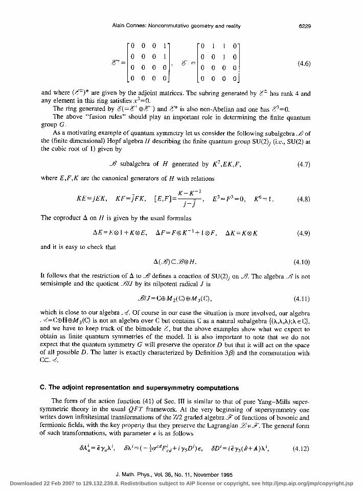
Alain Connes: Noncommutative geometry and reality 6229
(4.6)
and where (%+)* are given by the adjoint matrices. The subring generated by 5’ has rank 4 and any element in this ring satisfies x3=0.
The ring generated by Z( = g CBF) and P is also non-Abelian and one has Ks =O. The above “fusion rules” should play an important role in determining the finite quantum
group G. As a motivating example of quantum symmetry let us consider the following subalgebra J’ of
the (finite dimensional) Hopf algebra H describing the finite quantum group SU(2)j (i.e., SU(2) at the cubic root of 1) given by
& subalgebra of H generated by K2,EK,F,
where E, F, K are the canonical generators of H with relations
(4.7)
KE=jEK, KF=JFK, [E,F]=E, j-j
E3,F3,0, K6= 1. (4.8)
The coproduct A on H is given by the usual formulas
AE=E@l+K@E, AF=F@K-‘+1@F, AK=K@K (4.9)
and it is easy to check that
A(~cX?@H. (4.10)
It follows that the restriction of A to .W defines a coaction of SU(2)j on -6’. The algebra ./7/ is not semisimple and the quotient 3/J by its nilpotent radical J is
~/J=CCBM,(C)CBM,(C), (4.11)
which is close to our algebra &. Of course in our case the situation is more involved, our algebra . -&=C@N@M,(C) is not an algebra over C but contains C as a natural subalgebra {(A,X,X);XEC}, and we have to keep track of the bimodule E, but the above examples show what we expect to obtain as finite quantum symmetries of the model. It is also important to note that we do not expect that the quantum symmetry G will preserve the operator D but that it will act on the space of all possible D. The latter is exactly characterized by Definition 3fl) and the commutation with cc, T4.
C. The adjoint representation and supersymmetry computations
The form of the action function (41) of Sec. III is similar to that of pure Yang-Mills super- symmetric theory in the usual QFT framework. At the very beginning of supersymmetry one writes down infinitesimal transformations of the Z/2 graded algebra .F of functions of bosonic and fermionic fields, with the key property that they preserve the Lagrangian ZE.F. The general form of such transformations, with parameter E is as follows
SAL= &yak’, 6Xi=(-~c+CdFtd+i~sDi)~, SDi=Gy,(8+A)Xi, (4.12)
J. Math. Phys., Vol. 36, No. 11, November 1995 Downloaded 22 Feb 2007 to 129.132.239.8. Redistribution subject to AIP license or copyright, see http://jmp.aip.org/jmp/copyright.jsp

6230 Alain Connes: Noncommutative geometry and reality
where A is the vector potential, the X is a Fermion in the adjoint representation, and D is the auxiliary field.
We just want to point out that analogous formulas can be written in our general framework. Our auxiliary fields a of Eq (111.32) play the same role as the D of (12), the formula for 6A’ reads, up to normalization,
ax = BE, (4.13)
where we think of both X and E as vectors in the Hilbert space .%, 19 is the curvature (111.20) while E should satisfy extra conditions characterizing Killing spinors. The term which is more delicate to interpret is the variation SA since in (12) it invokes a bilinear expression EYJ’ in E and A. It is at this point that the real structure J on .A? plays a role. Indeed .% is now an .&bimodule (cf. Definition 3) and we can form the composition of correspondences (Ref. 8, Chap. V B),
3?@.&&.
Let T be the positive trace on ..d determined by Eq. (8) of Sec. III,
(4.14)
7(f)= f fk4, VfEA (4.15)
We assume that T is the restriction to . /% of a normal trace (still noted T) on the double commutant L 4” of. *Z. This is true in all relevant examples. Then by Ref. 8, Chap. V B.6 we have a natural bilinear map,
&E,H&3’-‘%, EE38, c$E33 (4.16)
of ZXZ to A%, &.%K Finally when .X (or rather .r=n, DomlDI”) is a finite projective module over &‘, we can identify (14) with the commutant c 4’ in .K of the right action of. 4, i.e., with endomorphisms of the right module .X over .A, with the inner product,
(T,,z-,)= f T,zy? (4.17)
By condition p) of Definition 3 all relevant operators, such as the vector potential A or the curvature 8 belong to the commutant . A’ of .T?? in .T so that an analog of the formula for & can now be written. We hope that these remarks will be useful in extending ideas of supersymmetry to our context, giving up of course the Z/2 graded commutativity underlying usual supersymmetry.
D. Towards curvature and Pontrjagin classes, the Levi-Civita spin connection We refer the reader to Refs. 10 and 24 for the development in our general framework of the
analog of the pseudodifferential calculus (based on the one parameter group ID 1 if. 1 D 1 i’ and ideas from the modular theory of operator algebras), of the Wodzicki residue (based on the notion of dimension spectrum) and of the local index formula. In the general framework of spectral triples the index formula, though local, is not yet in the explicit form given by polynomials in the analog of the Pontrjagin classes. It turns out however, that the Levi-Civita spin connection makes sense and is canonical in the general case of simple dimension spectrum. In the case of real spectral triples one should combine the ideas of Refs. 10 and 24 with those of Ref. 25 and also Ref. 7 in order to get curvature expressions for the local formula of Ref. 10 for the local cyclic cocycle index. Such computations ought to be a prerequisite for the understanding of the relation between the local and the global in noncommutative geometry as well as for the analog of the Einstein Hilbert gravity action.
We shall end these remarks by giving the general formula for the analog of the Levi-Civita spin connection in our framework. We let (h,.X,D) be a spectral triple of dimension p, with
J. Math. Phys., Vol. 36, No. 11, November 1995
Downloaded 22 Feb 2007 to 129.132.239.8. Redistribution subject to AIP license or copyright, see http://jmp.aip.org/jmp/copyright.jsp

Alain Connes: Noncommutative geometry and reality 6231
simple dimension spectrum, and denote by f the extension of the Dixmier trace to pseudodiffer- ential operators (cf. Ref. 10). Recall that given an element A =Cai[D,bi] of 0 the operator “dA”=~[D,ai][D,bi] is ambiguous, the ambiguity being an arbitrary auxiliary field PET The covariant differentiation VA is defined as the unique operator of the form
V,=+(DA+AD-“dA”)
such that the following orthogonality to 7 holds
(4.18)
f aV*P=O VffE9-I (4.19)
Condition (19) removes the ambiguity in (18). In the case of the Dirac spectral triple on a manifold one has
where Ox is the Levi-Civita spin connection evaluated on the vector field X dual to A, i.e., Xp=gp”Av.
We shall explore the general properties of V in a forthcoming paper.
’ D. Hilbert, Grundlagen der Geometrie (Teubner, Leipzig, 1899). Seventh edition, 1930. ‘H. Weyl, Philosophy of Mathematics and Natural Science (Princeton University, Princeton, NJ, 1949). ‘Weinberg, Gravitation and Cosmology (Wiley, New York, 1972). ‘T. Damour and J. H. Taylor, “Strong field tests of relativistic gravity and binary pulsars,” Phys. Rev. D 45, 1840-1868
(1992). s J. Frohlich, “The noncommutative geometry of two dimensional supersymmetric conformal field theory,” Preprint ETH
(1994). “S. Doplicher. K. Fredenhagen, and J. E. Roberts, “Quantum structure of space time at the Planck scale and Quantum
fields,” to appear in CMP. ‘K. Gawedzki and J. Frohlich, “Conformal Field theory and Geometry of Strings,” CRM proceedings and Lecture Notes,
7. 57-97 (1994). ‘A. Connes. Noncommutative geometry (Academic, New York, 1994). “J. Dixmier, Les C*-alghbres et leurs repr&entations (Gauthier Villars, Paris, 1964).
‘“A. Connes and H. Moscovici, “The local index formula in noncommutative geometry,” to appear in GAFA. “J. Milnor and D. Stasheff, Characteristic Classes. Ann. Math. Stud. 76 (Princeton University, Princeton, NJ, 1974). “M. E Atiyah. “K-theory and reality,” Quart. J. Math. Oxford 17, 367-386 (1966). ‘“G. Kasparov, “The operator K-functor and extensions of C*-algebras,” Izv. Akad. Nauk. SSSR Ser. Mat. 44, 571-636
(1980). lJA. R. Bernstein and F. Wattenberg, “Non-standard measure theory,” in Applications of model theory to algebra analysis
and probability, edited by W. A. J. Luxenburg (Holt, Rinehart, and Winston, New York, 1969). ‘“S. Power, “Hankel operators on Hilbert space,” Res. Notes in Math., 64 (Pitman, Boston, 1982). lbT P Branson and B. (brsted, “Explicit functional determinants in four dimensions,
(I.990 ” Proc. Am. Math. Sot. 113, 669-682
‘?T. P. Branson. “An anomaly associated with 4-dimensional quantum gravity,” to appear. ‘*V S . Vladimirov I V. Volovich, and E. I. Zelenov, p-adic analysis and mathemafical physics (World Scientific, Sin- , .
gapore, 1994). I9 A. Connes, D. Sullivan and N. Teleman, “Quasiconformal mappings, operators on Hilbert space, and local formulae for
characteristic classes,” ‘Topology 33, 663-681 (1994). ‘OS. P Novikov, “Topological invariance of rational Pontrjagin classes,” Doklady A.N. SSSR 163, 921-923 (1965). ” D. Sullivan, “Hyperbolic geometry and homeomorphisms, ” in Geometric Topology, Proceed. Georgia Topology Conf.,
Athens, Georgia (1977). pp. 543-555. “A. Connes and J. Lott, “Particle models and noncommutative geometry,” Nucl. Phys. B 18, Suppl. 29-47 (1990), (1991). ‘3M. F. Atiyah, K-Theory (Benjamin, New York, 1967). “A. Connes, “Geometry from the spectral point of view,” to appear in LMP. “A. H. Chamseddine, J. Frohlich, and 0. Grandjean, “The gravitational sector in the Connes-Lott formulation of the
standard model,” J. Math. Phys. 36, 6255-6275 (1995). “M. Wodzicki, Noncommutative residue, Part I. Fundamentals K-theory arithmetic and geometry, Lecture Notes in Math.
I289 (Springer, Berlin, 1987).
J. Math. Phys., Vol. 36, No. 11, November 1995 Downloaded 22 Feb 2007 to 129.132.239.8. Redistribution subject to AIP license or copyright, see http://jmp.aip.org/jmp/copyright.jsp