NONCONVEX MATRIX AND TENSOR RECOVERY WITH …

NONCONVEX MATRIX AND TENSOR RECOVERYWITH APPLICATIONS IN MACHINE LEARNING

BY MOHSEN GHASSEMI

A dissertation submitted to the

School of Graduate Studies

Rutgers, The State University of New Jersey

in partial fulfillment of the requirements

for the degree of

Doctor of Philosophy

Graduate Program in Electrical and Computer Engineering

Written under the direction of

Anand D. Sarwate

and approved by

New Brunswick, New Jersey

January, 2021

ABSTRACT OF THE DISSERTATION

Nonconvex Matrix and Tensor Recovery with

Applications in Machine Learning

by Mohsen Ghassemi

Dissertation Director: Anand D. Sarwate

This thesis focuses on some fundamental problems in machine learning that are posed

as nonconvex matrix factorizations. More specifically we investigate theoretical and

algorithmic aspects of the following problems: i) inductive matrix completion (IMC),

ii) structured dictionary learning (DL) from tensor data, iii) tensor linear regression

and iv) principal component analysis (PCA). The theoretical contributions of this thesis

include providing recovery guarantees for IMC and structured DL by characterizing the

local minima and other geometric properties of these problems. The recovery results

are stated in terms of upper bounds on the number of observations required to recover

the true matrix (dictionary in the case of DL) underlying the data. Another major

theoretical contribution of this work is providing fundamental limits on the performance

of tensor linear regression solvers by deriving a lower bound on the worst case mean

squared error of any estimator. On the algorithmic side, this thesis proposes novel

online and batch algorithms for solving structured dictionary learning problem as well

as a novel multi-stage accelerated stochastic PCA algorithm that achieves near optimal

results.

ii

Acknowledgements

I would like to express my deepest appreciation to my advisor, Prof. Anand Sarwate,

for his support, patience, encouragement, and invaluable guidance. It has been a true

pleasure working on many exciting and intellectually challenging problems under his

guidance. He has taught me everything I know about how to approach and solve

research problems, the value of mathematical rigor, and the art of presenting research

results in an accessible way.

I would also like to extend my sincere thanks to my thesis committee members Prof.

Waheed Bajwa, Prof. Mert Gurbuzbalaban, and Prof. Cunhui Zhang for reviewing my

work and their invaluable insights and suggestions. I must especially thank Waheed

who has been a mentor figure throughout my time at Rutgers and I have enjoyed

collaborating with him on many research projects. I am also grateful to Mert for his

guidance and collaboration on the work in Chapter 5 of this dissertation.

I was lucky to be surrounded with amazing friends and colleagues in Rutgers ECE

departments who were always there for me and with whom I enjoyed many interesting

discussion. I would specifically like to thank Zahra Shakeri, Haroon Raja, Talal Ahmed,

Mohammad Hajimirsadeghi, and Saeed Soori; spending the past 7 years in Rutgers

could not have been as much fun without them. Special thanks goes to my great friend

and colleague Zahra with whom I enjoyed collaborating on the work in Chapter 3. I am

also grateful to Baoul Taki who contributed to the work in Chapter 4. My thanks also

goes out to my lab members Hafiz Imtiaz, Sijie Xiong, and Konstantinos Nikolakakis

for their support and making my studies more enjoyable at Rutgers.

I have to thank my amazing parents and my brother Mohammad, without whom I

would never be where I am today. I cannot thank them enough for their immense love

and support. There is no way I can repay my parents for the countless sacrifices they

iii

have made for me. Finally, my very special thanks go out to my soulmate and best

friend Carolina. I am appreciative for her endless love and support. I would not have

survived graduate school without the joy she, and our dog Lucy, have brought to my

life.

iv

Dedication

For my parents and my grandma.

v

Table of Contents

Abstract . . . . . . . . . . . . . . . . . . . . . . . . . . . . . . . . . . . . . . . . ii

Acknowledgements . . . . . . . . . . . . . . . . . . . . . . . . . . . . . . . . . iii

Dedication . . . . . . . . . . . . . . . . . . . . . . . . . . . . . . . . . . . . . . . v

List of Tables . . . . . . . . . . . . . . . . . . . . . . . . . . . . . . . . . . . . . ix

List of Figures . . . . . . . . . . . . . . . . . . . . . . . . . . . . . . . . . . . . x

1. Introduction . . . . . . . . . . . . . . . . . . . . . . . . . . . . . . . . . . . 1

1.1. Motivation . . . . . . . . . . . . . . . . . . . . . . . . . . . . . . . . . . 1

1.2. Major Contributions . . . . . . . . . . . . . . . . . . . . . . . . . . . . . 2

2. Global Optimality in Inductive Matrix Completion . . . . . . . . . . . 5

2.1. Introduction . . . . . . . . . . . . . . . . . . . . . . . . . . . . . . . . . . 5

2.2. Problem Model . . . . . . . . . . . . . . . . . . . . . . . . . . . . . . . . 7

2.3. Geometric Analysis . . . . . . . . . . . . . . . . . . . . . . . . . . . . . . 10

2.4. Conclusion and Future Work . . . . . . . . . . . . . . . . . . . . . . . . 16

3. Learning Mixtures of Separable Dictionaries for Tensor Data . . . . 18

3.1. Introduction . . . . . . . . . . . . . . . . . . . . . . . . . . . . . . . . . . 18

3.1.1. Main Contributions . . . . . . . . . . . . . . . . . . . . . . . . . 20

3.1.2. Relation to Prior Work . . . . . . . . . . . . . . . . . . . . . . . 22

3.2. Preliminaries and Problem Statement . . . . . . . . . . . . . . . . . . . 23

3.3. Identifiability in the Rank-constrained LSR-DL Problem . . . . . . . . . 28

3.3.1. Compactness of the Constraint Sets . . . . . . . . . . . . . . . . 32

Adding the limit points . . . . . . . . . . . . . . . . . . . . . . . 33

vi

Eliminating the problematic sequences . . . . . . . . . . . . . . . 34

3.3.2. Asymptotic Analysis for Dictionary Identifiability . . . . . . . . 34

3.3.3. Sample Complexity for Dictionary Identifiability . . . . . . . . . 35

3.4. Identifiability in the Tractable LSR-DL Problems . . . . . . . . . . . . . 40

3.4.1. Regularization-based LSR Dictionary Learning . . . . . . . . . . 41

3.4.2. Factorization-based LSR Dictionary Learning . . . . . . . . . . . 42

3.4.3. Discussion . . . . . . . . . . . . . . . . . . . . . . . . . . . . . . . 45

3.5. Computational Algorithms . . . . . . . . . . . . . . . . . . . . . . . . . 45

3.5.1. STARK: A Regularization-based LSR-DL Algorithm . . . . . . . 46

3.5.2. TeFDiL: A Factorization-based LSR-DL Algorithm . . . . . . . . 48

3.5.3. OSubDil: An Online LSR-DL Algorithm . . . . . . . . . . . . . . 50

3.5.4. Discussion on Convergence of the Algorithms . . . . . . . . . . . 51

3.6. Numerical Experiments . . . . . . . . . . . . . . . . . . . . . . . . . . . 55


4. Tensor Regression . . . . . . . . . . . . . . . . . . . . . . . . . . . . . . . . 61

4.1. Introduction . . . . . . . . . . . . . . . . . . . . . . . . . . . . . . . . . . 61



4.2.1. Notation and Definitions . . . . . . . . . . . . . . . . . . . . . . . 64

4.2.2. Low-Rank Tensor Linear Regression . . . . . . . . . . . . . . . . 65

4.2.3. Minimax Risk . . . . . . . . . . . . . . . . . . . . . . . . . . . . . 67

4.3. Minimax Risk of Tensor Linear Regression . . . . . . . . . . . . . . . . . 68

4.3.1. Our Approach . . . . . . . . . . . . . . . . . . . . . . . . . . . . 69

4.3.2. Main Result . . . . . . . . . . . . . . . . . . . . . . . . . . . . . . 71

4.3.3. Discussion . . . . . . . . . . . . . . . . . . . . . . . . . . . . . . . 75


4.5. Proofs . . . . . . . . . . . . . . . . . . . . . . . . . . . . . . . . . . . . . 77

vii

5. Momentum-based Accelerated Streaming PCA . . . . . . . . . . . . . 89

5.1. Introduction . . . . . . . . . . . . . . . . . . . . . . . . . . . . . . . . . . 89



5.2.1. Notation and Definitions . . . . . . . . . . . . . . . . . . . . . . . 94

5.2.2. The stochastic PCA problem . . . . . . . . . . . . . . . . . . . . 94

5.2.3. Baseline Stochastic PCA Algorithms . . . . . . . . . . . . . . . . 95

5.2.4. Momentum-based Acceleration of Gradient-based Optimization

Methods . . . . . . . . . . . . . . . . . . . . . . . . . . . . . . . . 95

5.3. Oja’s Rule with Heavy Ball Acceleration with Fixed Step Size . . . . . . 97

5.4. Multistage HB Accelerated PCA . . . . . . . . . . . . . . . . . . . . . . 109


Bibliography . . . . . . . . . . . . . . . . . . . . . . . . . . . . . . . . . . . . . 119

6. Appendix . . . . . . . . . . . . . . . . . . . . . . . . . . . . . . . . . . . . . 137

6.1. The Rearrangement Procedure . . . . . . . . . . . . . . . . . . . . . . . 137

6.1.1. Kronecker Product of 3 Matrices . . . . . . . . . . . . . . . . . . 138

6.1.2. The General Case . . . . . . . . . . . . . . . . . . . . . . . . . . 140

6.2. Properties of the Polynomial Sequence . . . . . . . . . . . . . . . . . . . 142

viii

List of Tables

3.1. Table of commonly used notation in Chapter 3 . . . . . . . . . . . . . . 29

3.2. Performance of DL algorithms for image denoising in terms of PSNR . . 56

3.3. Performance of TeFDiL with various ranks for image denoising in terms

of PSNR . . . . . . . . . . . . . . . . . . . . . . . . . . . . . . . . . . . . 56

ix

List of Figures

3.1. Dictionary atoms for representing RGB image Barbara for separation

rank (left-to-right) 1, 4, and 256. . . . . . . . . . . . . . . . . . . . . . . 19

3.2. Example of rearranging a Kronecker structured matrix (N = 3) into a

third order rank-1 tensor. . . . . . . . . . . . . . . . . . . . . . . . . . . 30

3.3. (a) Normalized representation error of various DL algorithms for 3rd-

order synthetic tensor data. (b) Performance of online DL algorithms

for House. . . . . . . . . . . . . . . . . . . . . . . . . . . . . . . . . . . . 57

5.1. Performance of our proposed method and standard Oja’s method in

terms of error (1 − u>1 wt‖u>1 wt‖2

) versus the number of iterations on a syn-

thetic dataset. We can see improvement in the performance of our pro-

posed heavy-ball momentum accelerated method compared to the stan-

dard non-accelerated method. . . . . . . . . . . . . . . . . . . . . . . . . 92

6.1. Rearranging a Kronecker structured matrix (N = 2) into a rank-1 matrix.138

6.2. Example of rearranging a Kronecker structured matrix (N = 3) into a

third order rank-1 tensor. . . . . . . . . . . . . . . . . . . . . . . . . . . 141

x

1

Chapter 1

Introduction

1.1 Motivation

Many fundamental problems in machine learning, statistics, and signal processing can

be seen as matrix estimation problems. Examples of such problems include matrix

sensing [1, 2], matrix completion [3–5], phase retrieval [6, 7], dictionary learning [8, 9],

principal component analysis (PCA) [10], robust PCA [11], and blind deconvolution

[12]. One common approach to solving these problems is resorting to convex relaxations

and applying well-known convex optimization methods. While convexified formulations

allow for employing well-established analytical tools to provide statistical performance

guarantees for these problems, the computational cost and storage requirement of con-

vex optimization methods makes them unsuitable for large-scale problems. Nonconvex

matrix factorization schemes on the other hand enjoy lower storage requirements and

per-iteration computational cost, and are amenable to parallelization. With prevalence

of big data, these properties have become more important than ever since information

processing and learning applications often involve dealing with high dimensional and/or

high volume data, resulting in large-scale matrix factorization problems. Emergence

of such large-scale problems necessitates development of efficient matrix factorization

methods whose computational and storage costs scale favorably with matrix dimensions.

This thesis focuses on providing theoretical guarantees as well as developing efficient

algorithms for some fundamental matrix factorization problems with applications in

representation learning, recommendation systems, and other areas of machine learning.

2

1.2 Major Contributions

In this body of work we study three problems that can be formulated as nonconvex

matrix decomposition problems. We first provide theoretical recovery guarantees for

inductive matrix completion (IMC) by characterizing its optimization landscape.

Then, we propose a novel structured dictionary learning model for learning sparse

representations of tensor data and develop theory and numerical algorithms to validate

the usefulness of this model. We also study the fundamental limits of estimation in

a tensor linear regression problem and demonstrate the benefits of preserving the

tensor structure of data and exploiting multi-directional interdependence among model

variables in this problem. Finally, we develop a momentum-based accelerated algo-

rithms for the streaming principal component analysis (PCA) problem and study

the impact of introducing a momentum term in to a classic solver of this nonconvex

problem. A more detailed overview is provided in the following.

In Chapter 2, we present our first major contribution. That is, we provide re-

covery guarantees for inductive matrix completion (IMC), a powerful technique with

applications recommendation systems with side information. The aim of IMC is to

reconstruct a low-rank matrix from a small number of given entries by exploiting the

knowledge of the feature spaces of its row and column entities. We study the opti-

mization landscape of this nonconvex problem and show that given sufficient number of

observed entries, all local minima of the problem are globally optimum and all saddle

points are “escapable”. The immediate consequence of this result is that any first order

optimization method such as gradient decent can be used to recover the true matrix.

Moreover, we characterize how the knowledge of feature spaces reduces the number of

required observed entries to recover (identify) the true matrix.

Our second main contribution, presented in Chapter 3, focuses on sparse repre-

sentation learning for tensor (multidimensional) data. To this end, we study dictionary

learning (DL), an effective and popular data-driven technique for obtaining sparse rep-

resentations of data [8, 13], for tensor data. Traditional dictionary learning methods

treat tensor data as vector data by collapsing each tensor to a vector. This disregards

3

the multidimensional structure in tensor data and results in dictionaries with large

number of free parameters. With the increasing availability of large and high dimen-

sional data sets, it is crucial to keep sparsifying models reasonably small to ensure their

scalable learning and efficient storage. Our focus in this work is on learning of compact

DL models that yield sparse representations of tensor data. Recently, some works have

turned to tensor decompositions such as the Tucker decomposition [14] and CANDE-

COMP/PARAFAC decomposition (CPD) [15] for learning of structured dictionaries

that have fewer number of free parameters. In particular, separable DL reduces the

number of free parameters in the dictionary by assuming that the transformation on

the sparse signal can be be implemented by performing a sequence of separate trans-

formations on each signal dimension [16]. While separable DL methods enjoy lower

sample/computational complexity and better storage efficiency over traditional DL [17]

methods, the separability assumption among different modes of tensor data can be

overly restrictive for many classes of data [18], resulting in an unfavorable trade-off

between model compactness and representation power. In this work, we overcome this

limitation by proposing a generalization of separable DL that we interchangeably refer

to as learning a mixture of separable dictionaries or low separation rank DL (LSR-DL).

This model provides better representation power than the separable model while hav-

ing smaller number of parameters than traditional DL by allowing for increasing the

number of parameters in structured DL in a consistent manner. To show the usefulness

of our proposed model, we study the identifiability of the underlying dictionary in this

model and derive the sufficient number of samples for local identification of the true

dictionary under the LSR-DL model. Our results show that while the sample com-

plexity of LSR-DL is slightly higher sample complexity than that of separable DL, it

can still be significantly lower than that of traditional DL. We further develop efficient

batch and online numerical algorithms to solve the LSR-DL problem.

Our third main contribution, which appears in Chapter 4, focuses on using an

information theoretic approach to derive minimax risk (best achievable performance

in the worst case scenario) of estimating the true parameter variables in a linear re-

gression problem with tensor-structured data. Our results show a reduction in sample

4

complexity required for achieving a target worst case risk compared to the case where

the data samples are treated as vectors and thus demonstrate the benefits of preserv-

ing the spatial structure of data and exploiting the multi-directional interdependence

among model variables in the tensor linear regression model.

Finally, in Chapter 5, we present our fourth contribution. In this chapter we

study the principal component analysis (PCA) problem when data arrives in a stream-

ing fashion. We investigate the effect of adding a momentum term to the update rule

of well-known stochastic PCA algorithm called Oja’s method. While the efficacy of

momentum-based acceleration for stochastic algorithms is not well-established in gen-

eral, our proposed multi-stage accelerated variant of Oja’s method achieves near opti-

mal convergence rate in both in both noiseless case (bias term) and noisy case (variance

term).

5

Chapter 2

Global Optimality in Inductive Matrix Completion

2.1 Introduction

Matrix completion [3, 19] is an important technique in machine learning with applica-

tions in areas such as recommendation systems [20] or computer vision [21]. The task

is to reconstruct a low-rank matrix M∗ ∈ Rn1×n2 from a small number of given entries.

Theoretical results in the literature show that the number of required samples for ex-

act recovery is O(rn log2 n) where n = n1 + n2 and r = rank(M∗) [22, 23]. In some

applications, the algorithm may have access to side information that can be exploited

to improve this sample complexity. For example, in many recommendation systems

where the given entries of M∗ represent the ratings given by users (row entities) to

items (column entities), the system has additional information about both user profiles

and items.

Among the many approaches to incorporate side information [24–30], inductive ma-

trix completion (IMC) [24, 25] models side information as knowledge of feature spaces.

This is incorporated in the model by assuming that each entry of the unknown matrix

of interest M∗ ∈ Rn1×n2 is in form of M∗ij = xTi W∗yj , where xi ∈ Rd1 and yj ∈ Rd2

are known feature vectors of i-th row (user) and j-th column (item), respectively. The

low-rank matrix completion problem in this case can be formulated as recovering a

rank-r matrix W∗ ∈ Rd1×d2 such that the observed entries are Mij = xTi W∗yj . In

fact, the IMC problem translates to finding missing entries of M∗ as recovering matrix

W∗ from its measurements in form of xiW∗yj =

⟨xiy

Tj ,W

∗⟩

for (i, j) ∈ Ω.

Using this model, the sample complexity decreases considerably if the size of matrix

M is much larger than W∗. Another advantage of this model is that rows/columns of

the unknown matrix can be predicted without knowing even one of their entries using

6

the corresponding feature vectors once we recover W∗ using the given entries. This is

not possible in standard matrix completion since a necessary condition for completing a

rank-r matrix is that at least r entries of every row and every column are observed [3].

The nonconvex rank-r constraint makes the problem challenging. There are two

main approaches in the matrix recovery literature to impose the low-rank structure in

a tractable way. The first approach is using convex relaxations of the nonconvex rank-

constrained problem [3, 11, 23, 31–33]. In the IMC problem, at least O(rd log d log n)

samples are required for recovery of W∗ using a trace-norm relaxation, where d =

d1 +d2 [24, 25]. The trace-norm approach has also been proposed for the IMC problem

with noisy features where the unknown matrix is modeled as XW∗YT +N where the

residual matrix N models imperfections and noise in the features [27].

Another approach uses matrix factorization, where the d1 × d2 matrix W is ex-

pressed as W = UVT , where U ∈ Rd1×r and V ∈ Rd2×r [20, 34]. Jain et al. show

that alternating minimization (AM) converges to the global solution of matrix sens-

ing and matrix completion problems in linear time under standard conditions [34].

Inspired by this result, Zhong et al. [25] show that for the factorized IMC problem,

O(r3d log dmaxr, log n) samples are sufficient for ε-recovery of W∗ using AM.

On the computational side, the per-iteration cost of the solvers of the convex matrix

estimation problem is high since they require finding the SVD of a matrix in case of

implementing singular value thresholding [35] or proximal gradient methods [36], or

they involve solving a semi-definite program. On the other hand, both empirically

and theoretically, stochastic gradient descent (SGD) and AM have been shown to find

good local optima in many nonconvex matrix estimation problems and that suitable

modifications to the objective function can find global optima [34, 37]. These simple

local search algorithms have low memory requirement and per-iteration computational

cost, due to the fact that in low-rank problems r d1, d2. Although the IMC model

reduces the dimensionality of the matrix estimation problem from n1 × n2 to d1 × d2,

the lower complexity of the solvers of the factorized model is appealing [25].

On the theoretical side, the trace-norm based model is intriguing in that it allows

for employing well-established tools to analyze the statistical performance of the convex

7

program. Although the matrix factorization based models in general are theoretically

less understood, recent works have studied the optimization landscape of some of these

nonconvex problems and show that their objective functions are devoid of “poor” local

minima. Problems such as matrix completion [4, 5], matrix sensing [1, 2], phase re-

trieval [7], deep (linear) neural networks [38, 39] are amenable to this approach. To the

best of our knowledge, this work is the first to study the geometry and the statistical

performance of IMC under the factorized model.

The work in this chapter is motivated by the recovery guarantees of AM for the

(nonconvex) factorized IMC problem. Our key technical contribution is to use con-

centration inequalities to show that given a sufficient number of measurements, the

ensemble of sensing matrices xiyTj almost preserves the energy of all rank-2r matrices,

i.e. it satisfies restricted isometry property of order 2r. This allows us to use the frame-

work of Ge et al. [5] for matrix sensing problems. Our final result is that given at least

O(drmaxr2, log2 n) observations, in the (regularized) factorized IMC problem i) all

local minima are globally optimal, ii) all local minima fulfill UVT = W∗, and iii) the

saddle points are escapable in the sense that the Hessian at those points has at least

one negative eigenvalue.

Our result implies that the success of AM in the nonconvex IMC problem is to some

degree a result of the geometry of the problem and not solely due to the properties of

the algorithm. In fact, any algorithm with guaranteed convergence to a local minimum,

e.g. SGD [37], can be used for solving the factorized IMC problem.1

2.2 Problem Model

Notation and Definitions. Throughout this chapter, vectors and matrices are, re-

spectively, denoted by boldface lower case letters: a and boldface upper case letters: A.

We denote by Aij the j-th element of the i-th row of A. The smallest eigenvalue of A

is denoted by λmin(A). In matrix completion, the set of indices of the observed (given)

entries of an incomplete matrix A ∈ Rn1×n2 is denoted by Ω with size m = |Ω|. Also,

1The results presented in this chapter have been published in Proceedings of 2018 IEEE InternationalConference on Acoustics, Speech and Signal Processing [40]

8

AΩ denotes the linear projection of A onto the space of n1×n2 matrices whose entries

outside Ω are zero. The inner product of two matrices is defined as 〈A,B〉 = Tr(ATB).

In a noncovex optimization problem, a poor local minimum is a local minimum which

is not globally optimum.

We repeatedly use the (matrix) restricted isometry property (RIP) [31] and the strict

saddle property [37, 41] defined below.

Definition 1. A linear operator A(·) : Rd1×d2 → Rm satisfies r-RIP with δr RIP

constant if for every W ∈ Rd1×d2 such that rank(W ) ≤ r it holds that

(1− δr) ‖W‖2F ≤ ‖A(W)‖22 ≤ (1 + δr) ‖W‖2F .

Definition 2. A twice differentiable function f(x) is strict saddle if λmin

(∇2f(x)

)< 0

at its saddle points.

Inductive Matrix Completion. Consider the nonconvex low-rank matrix completion

problem

minM∈Rn1×n2

‖M∗Ω −MΩ‖2F s.t. rank(M) ≤ r. (2.1)

In an inductive matrix completion problem, the underlying matrix has the form M∗ =

XW∗YT where the side information matrices X ∈ Rn1×d1 and Y ∈ Rn2×d2 are known

and W∗ = U∗V∗T with U∗ ∈ Rd1×r, V∗ ∈ Rd2×r is unknown. Therefore, the problem

can be written as

minW∈Rd1×d2

∥∥(M∗ −XWYT)

Ω

∥∥2

F

s.t. rank(W) ≤ r. (2.2)

This problem can be reformulated into an unconstrained nonconvex problem by ex-

pressing W as UVT , where U ∈ Rd1×r, V ∈ Rd2×r:

minU,V

f(U,V) =∥∥(M∗ −XUVTYT

)Ω

∥∥2

F+R (U,V) (2.3)

9

The regularization term R(U,V) is added to account for the invariance of the asymmet-

ric factorized model to scaling of the factor matrices by reciprocal values. A common

choice that suits our model is R(U,V) = 14‖UUT −VVT ‖2F [2, 5].

The objective function f(U,V) in problem (2.3) alternatively can be written as

f(U,V) =∑

(i,j)∈Ω

(M∗

ij −⟨xiy

Tj ,UVT

⟩)2+

1

4

∥∥UUT −VVT∥∥2

F,

where xTi and yTj respectively are the ith and jth rows of X and Y. Observe that⟨xiy

Tj ,UVT

⟩= xTi UVTyj .

This shows that the IMC problem (2.3) can be thought of as a matrix sensing

problem where we are given linear measurements of the d1 × d2 matrix W∗ by sensing

matrices Aij = xiyTj . Define the linear operator A such that A(W) is a vector whose

elements are the measurements 1√m〈Aij ,W〉.

In this chapter, we make the following assumptions regarding the side information

matrices and the sampling model.

Assumption 1 (Side information). The side information matrices satisfy XTX =

n1Id1 and YTY = n2Id2.2 We also make the assumption that for any given matrices

U and V with orthogonal columns, the rows of the side information matrices (feature

vectors) satisfy∥∥Uxi

∥∥2

2≤ µr and

∥∥Vyj∥∥2

2≤ µr, where r = max(r, log n1, log n2) and µ

is a positive constant. This assumption, for example, is satisfied with high probability

when the side information matrices X and Y are instances generated from a random

orthonormal matrix model (the first d1 (respectively d2) columns) and rescaled by√n1

(respectively√n2) [3, 25].

Assumption 2 (Sampling model). Indices i and j are independent and uniformly

distributed on 1, 2, . . . , n.

2This is not a restrictive assumption since we can apply orthonormalization methods such as Gram-Schmidt process [42] and then rescale to ensure this assumption is satisfied.

10

2.3 Geometric Analysis

We are interested in the geometric landscape of the objective function in the IMC prob-

lem (2.3). We will show that simple algorithms like AM can recover the true underlying

matrix with arbitrary accuracy because given enough observations, the objective func-

tion in this problem i) has no poor local minima, ii) has only local minima which satisfy

UVT = W∗, and iii) is strict saddle.

We employ the framework developed by Ge et al. [5] for matrix sensing to show

that the objective function of the IMC problem (2.3) satisfies properties i), ii), and

iii). Theorem 1 states the main result of this chapter.

Theorem 1. Consider the IMC problem (2.3) seen as a matrix recovery problem with

sensing matrices Aij = xiyTj for (i, j) ∈ Ω, such that Assumptions 1 and 2 hold.

Let r = maxr, log n1, log n2. If the number of measurements is m = O(µ2dr2r

), then

there exists a positive constant h such that with probability higher than 1−2 exp (−hm),

the nonconvex objective function f(U,V) has the following properties: i) all its local

minima are globally optimal , ii) all its local minima satisfy UVT = M∗, and iii) it

satisfies the strict saddle property.

The proof strategy here is to show that at any stationary point of f(U,V) (and its

neighborhood), the “difference” ∆ between the point and the true solution (which is

basically the Euclidian distance between the point and its nearest global minimum) is

a descent direction. This means that (U,V) cannot be local minimum unless ∆ = 0

(no poor local minima and exact recovery) and that the Hessian at the saddle points

cannot be positive semidefinite (strict saddle property). To this end, following the

proposed strategy by Ge, Jin, and Zheng [5], we construct B =

U

V

∈ R(d1+d2)×r,

W = UVT , and N = BBT and reformulate problem (2.3) as the positive semidefinite

(PSD) low-rank matrix recovery problem

minB

f(B) = ‖T (N ∗)− T (BBT )‖22. (2.4)

11

where B∗ =

U∗

V∗

, N ∗ = B∗B∗T , and T is a linear operator such that T (N ) is an

ensemble of m measurements 〈Tij ,N〉 such that

〈Tij ,N〉2 =1

m

(4 〈Aij ,W〉2 + ‖UUT −VVT ‖2F

).

The following definition captures the invariance of the solution of symmetric matrix

recovery to rotation, negation, or column permutation.

Definition 3. Given matrices B,B∗ ∈ Rd×r, define the rotation invariant difference

∆(B; B∗) , B−B∗D, where D = argminZ:ZZT=ZTZ=Ir

‖B−B∗Z‖2F .

We use the shorthand ∆ for ∆(B; B∗) in the rest of this chapter. The second

order term in the Taylor expansion of f(B) becomes dominant in the neighborhood of

stationary points. Therefore it suffices to show that δT∇2f(B)δ, where δ = vec(∆),

is strictly negative for points in these regions, except when ∆ = 0, to prove that ∆

is a descent direction. Theorem 2 states that if linear operator B is RIP, then we can

show δT∇2f(B)δ is strictly negative in the neighborhood of stationary points unless

they correspond to N ∗ (and its submatrix W∗) and consequently M∗ = XW∗YT , the

ground truth matrix in problem (2.3).

Theorem 2. Consider the objective function of the PSD matrix recovery problem

(2.4). If the measurement operator T satisfies (2r, δ2r)-RIP, then any point satisfy-

ing ‖∇f(B)‖F ≤ ξ, the quadratic form δT∇2f(B)δ for δ = vec(∆) defined above is

negative unless ‖∆‖F ≤ Kξ/ (1− 5δ2r) for some positive constant K.

Proof sketch. The proof is based on the following equality (Lemma 7 in [5]):

δT∇2f(B)δ =∥∥T (∆∆T

)∥∥2

2− 3 ‖T (N −N ∗)‖22 + 4 〈∇f(B),∆〉 . (2.5)

Using the RIP property of T , which implies that the measuring operator captures

the energy of the observed matrix with small deviation, and applying the bounds

12

∥∥∆∆T∥∥2

F≤ 2 ‖N −N ∗‖2F and k ‖∆‖2F ≤ ‖N −N ∗‖

2F (Lemma 6 in [5]) results in

δT∇2f(B)δ ≤ −k (1− 5δ2r) ‖∆‖2F + 4ξ ‖∆‖F . (2.6)

Therefore the bilinear form on the left cannot be nonnegative unless we have ‖∆‖2F ≤

4ξ/ (k (1− 5δ2r)).

Now, we show that the linear operator A and consequently T are 2r-RIP. Note that

it is important that we show 2r-RIP rather that r-RIP because in Theorem 2, T is

applied to B − B∗ which can be of rank at most 2r. It also guarantees that the null

space of T does not include any matrices of rank 2r or less, which is a necessary and

sufficient condition for unique recovery [43, 44].

Theorem 3. Consider the IMC problem (2.3) seen as a matrix recovery problem with

sensing matrices Aij = xiyTj for (i, j) ∈ Ω, such that Assumptions 1 and 2 hold. If the

number of measurements m = O(µ2dr2r log(36

√2/δ)/δ2

), then there exists a positive

constant h such that with probability higher than 1 − 2 exp (−hm), the linear operator

A(·), seen as an ensemble of m measurements 1√m〈Aij , ·〉, is 2r-RIP with RIP constant

δ2r = 2δ.

Proof. We show that∥∥A(W)

∥∥2

2is close to

∥∥W∥∥2

Ffor all rank-2r matrices W, i.e.,∣∣∥∥A(W)

∥∥2

2−∥∥W∥∥2

F

∣∣ ≤ δ2r

∥∥W∥∥2

F. We use Bernstein’s inequality to find a bound on

the deviation of the sum of m random variables 1√m

⟨xiy

Tj ,W

⟩from their mean

∥∥W∥∥2

F

for a given rank-2r matrix W. This is formally stated in Lemma 1. Then we find a

similar bound for all rank-2r (or less) matrices.

Lemma 1. Consider the same setting as Theorem 3. For a given matrix W of rank

2r, with probability at least 1− C exp (−cm), for some positive constatnts C and c, we

have

(1− δ2r)∥∥W∥∥2

F≤∥∥A(W)∥∥2

2≤ (1 + δ2r)

∥∥W∥∥2

F.

13

Proof of Lemma 1. In order to show that the average random measurement, denoted

by ‖A(W)‖22 = 1

m

∑ij〈Aij ,W〉2, is close to its expectation ‖W‖2F , we use Bernstein’s

inequality [45]:

P(∣∣Z − ηZ∣∣ > ε

)≤ 2 exp

( −mε2/21m

∑ij Var(Zij) +BZε/3

),

where Z = 1m

∑ij Zij and ηZ is the mean of the random variables. To apply Bernstein’s

inequality, we need to find the expectation, the variance (or an upper bound on the

variance), and an upper bound on the absolute value of the random variables in the

summand, denoted by Zij = xTi WyjyTj Wxi. Note that X and Y are known orthogonal

matrices and the only source of randomness is the choice of (i, j). First, we find the

mean of the random variables:

ηZ = E[xTi Wyjy

Tj Wxi

]= E

[eTi XUV

TYT eje

Tj YWTXT ei

]= E

[Tr(VTYT eje

Tj YWTXT eie

Ti XU

)]= Tr

(VTYTE

[eje

Tj

]YWTXTE

[eie

Ti

]XU

)(a)= Tr

(VTYTYWTXTXU

)(b)= Tr

(VTWT U

)= Tr

(UVT · WT

)=∥∥W∥∥2

F, (2.7)

where W = UVT , equality (a) follows from E[eie

Ti

]= 1

n1In1 and (b) follows from

Assumption 1. Next we find an upper bound BZ on |Zij |:

|Zij | = ·xTi UΣVTyj · yTj UΣV

Txi

≤(∥∥∥xTi U

∥∥∥2

∥∥∥Σ∥∥∥2

∥∥∥VTyj

∥∥∥2

)2

= σ21

∥∥∥VTyj

∥∥∥2

2·∥∥∥UTxi

∥∥∥2

2

≤ r2µ2σ21, (2.8)

14

where UΣVT

is the SVD of W, σ1 = ‖W‖2, and the last inequality follows from

Assumption 1. Finally, for the variance of the random variables we have

1

m

∑ij

Var(Zij) ≤1

m

∑ij

E[Z2ij

](a)

≤ 1

mBz∑ij

E [Zij ]

≤ r2µ2σ21‖W‖2F , (2.9)

where inequality (a) is due to the fact that Zij ’s are nonnegative random variables.

Using Bernstein’s inequality we get the following.

P(∣∣‖A(W)‖22 − ‖W‖2F

∣∣∣ > ε)≤ 2 exp

(− mε2/2

1m

∑ij Var(Zij) +BZε/3

)

≤ 2 exp

(− mε2/2

r2µ2σ21‖W‖2F + r2µ2σ2

1ε/3

). (2.10)

Set ε = δ ‖W‖2F . We have

P(∣∣‖A(W)‖22 − ‖W‖2F

∣∣ > δ‖W‖2F)≤ 2 exp

(−

mδ2‖W‖2F /2r2µ2σ2

1(1 + δ/3)

)

≤ 2 exp

(− mδ2/2

µ2r2(1 + δ/3)

). (2.11)

Set δ =

√4µ2r2 log(2/ρ)

m . If m > 4µ2r2 log(2/ρ) we have δ < 1. Therefore,

P(∣∣∣‖A(W)‖22 − ‖W‖2F

∣∣∣ > δ‖W‖2F)≤ 2 exp

(− mδ2

4µ2r2

).

This concludes the proof of Lemma 1.

Now we return to the proof of Theorem 3. The rest of the proof is based on Theorem

2.3 in [46]. We showed in Lemma 1 that for a given matrix of rank at most 2r,

P(∣∣∣‖A(W)‖22 − ‖W‖2F

∣∣∣ > δ‖W‖2F)≤ C exp(cm),

15

for positive constants C and c. In order to extend the result such that a similar

result holds for all rank-2r (or less) matrices, we use the union bound for an ε-net

3 [47] of the space of such matrices with unit Frobenius norm. For the set Sd2r =

W ∈ Rd×d : rank(W) ≤ 2r,∥∥∥W∥∥∥

F= 1, there exists an ε′-net Sd2r ⊂ Sd2r such that

|Sd2r| ≤ (9/ε′)(2d+1)2r [43, 46]. It follows from 2.12 and the union bound that

P(

max¯W∈Sd2r

∣∣∣ ∥∥∥A(W)∥∥∥2

2− 1∣∣∣ > δ

)≤ |Sd2r|C exp(−cm).

Setting ε′ = δ/(4√

2) results in

P(

max¯W∈Sd2r

∣∣∣ ∥∥∥A(W)∥∥∥2

2− 1∣∣∣ > δ

)≤ C exp

((2d+ 1)2r log(36

√2/δ)− cm

)= C exp

(c′dr − cm

)≤ C exp (−hm) , (2.12)

where c′ = 6 log(36√

2/δ) and h = c − c′/(K). We need m > Kdr so that the last

inequality above holds, and we need K > c′/c so that h becomes positive. This means

that m > c′dr/c. Plugging in the values for C, c, and c′, we get that if with probability

at least 1− 2 exp (−hm),

max¯W∈Sd2r

∣∣∣∣∥∥∥A(W)∥∥∥2

2− 1

∣∣∣∣ ≤ δ.It follows from this bound that for all W of rank at most 2r that with probability at

least 1− 2 exp (−hm) [46],

1− 2δ ≤

∥∥∥∥∥A( W

‖W‖2F

)∥∥∥∥∥2

2

≤ 1 + 2δ.

3An ε-net is a set of points such that the union of radius-ε balls centered at these points covers thespace

16

Since A is a linear operator, for all W with rank(W) ≤ 2r,

(1− 2δ) ‖W‖2F ≤ ‖A(W)‖22 ≤ (1 + 2δ) ‖W‖2F .

This means that A is 2r-RIP with δ2r = 2δ when m = O(µ2dr2r log(36

√2/δ)/δ2

).

Finally, we show that the sensing operator T is RIP on (d1 + d2) × (d1 + d2) PSD

matrices of rank at most 2r. Any of these PSD matrices can be written in form of

N =

UUT UVT

VT U VVT

where U ∈ Rd1×2r and V ∈ Rd2×2r. We defined T such that

T (N ) = 4A(UVT ) +∥∥UUT

∥∥2

F+∥∥VVT

∥∥2

F− 2∥∥W∥∥2

Fwhere W = UVT . Since

‖N‖2F =∥∥UUT

∥∥2

F+∥∥VVT

∥∥2

F+ 2∥∥W∥∥2

F,

if we have

(1− δ)∥∥W∥∥2

F≤∥∥A(W)

∥∥2

2−∥∥W∥∥2

F≤ (1 + δ)

∥∥W∥∥2

F,

then it follows that

(1− 2δ)∥∥N∥∥2

F≤∥∥T (N )

∥∥2

2−∥∥N∥∥2

F≤ (1 + 2δ)

∥∥N∥∥2

F.

Note that the deduction of the RIP of T from the RIP of A is thanks to the choice of

the regularizer in (2.3).

2.4 Conclusion and Future Work

In this chapter, we discussed the geometric landscape of the inductive matrix completion

(IMC) problem. The IMC model incorporates the side information in form of features of

the row and column entities (xi’s and yj ’s) and can be formulated as a low-rank matrix

recovery problem where each observed entry of M∗ = XW∗Y is seen as a measurement

of W∗, that is M∗ij = xTi W∗yj . Motivated by the recovery guarantees of local search

algorithms like AM for the factorized IMC problem [25], we study the optimization

landscape of the factorized IMC problem. Using a framework developed by Ge et al. [5]

17

for matrix sensing problems, we show that, given O(maxr2, log2 nrd) observations,

for the (regularized) factorized IMC problem i) there are no poor local minima, ii) the

global minima satisfy UVT = W∗, iii) The Hessian at the saddle point has at least

one negative eigenvalue.

This result shows that the recovery guarantees of AM in the IMC problem is not

merely due to the algorithm and the geometry of the problem plays an important role.

In fact, any algorithm, such as SGD, that can efficiently escape saddle points and find

a local minimum can be used for solving the factorized IMC problem.

The IMC model has been studied extensively in the recent years. It has been

employed in a variety of applications [48–51] and has been extended to more general

settings such as IMC with noisy side information [27], high rank IMC [52], and non-

linear IMC [53]. However, there are still many possible directions that have not yet

been adequately explored. For example, tensor completion with side information is an

area that although has received some attention in the recent years. A natural way to

extend the IMC model to tensors is based on Tucker tensor decomposition. The Tucker

decomposition factorizes an N -way tensor M ∈ Rn1,n2,··· ,dN in the following manner:

M = W ×1 U1 ×2 U2 ×3 · · · ×N UN ,

where W ∈ Rp1×p2×···×pN denotes the core tensor, Un ∈ Rdn×pn denote factor matrices

along the n-th mode of A for n ∈ [N ] and ×n denotes the mode-n product between a

tensor and a matrix. Similar to inductive matrix completion, in many cases we have

side information in form of feature matrices for the n mode entities, i.e. knowledge

of the latent spaces of the underlying tensor. While there are a few recent works

that explore this approach to incorporate side information into tensor completion [54–

56], our understanding of this problem in terms of sample complexity, optimization

landscape, and many other aspects is limited. While we leave extension the study of

tensor completion with side information to future work, in the next chapter we employ

some of the analytical tools that we use in Chapter 2 to provide recovery guarantees

for a tensor problem, namely structured dictionary learning for tensor data.

18

Chapter 3

Learning Mixtures of Separable Dictionaries for Tensor

Data

3.1 Introduction

Many data processing tasks such as feature extraction, data compression, classification,

signal denoising, image inpainting, and audio source separation make use of data-driven

sparse representations of data [8, 9, 13]. In many applications, these tasks are performed

on data samples that are naturally structured as multiway arrays, also known as mul-

tidimensional arrays or tensors. Instances of multidimensional or tensor data include

videos, hyperspectral images, tomographic images, and multiple-antenna wireless chan-

nels. Despite the ubiquity of tensor data in many applications, traditional data-driven

sparse representation approaches disregard their multidimensional structure. This can

result in sparsifying models with a large number of parameters. On the other hand,

with the increasing availability of large data sets, it is crucial to keep sparsifying models

reasonably small to ensure their scalable learning and efficient storage within devices

such as smartphones and drones.

Our focus in this chapter is on learning of “compact” models that yield sparse

representations of tensor data. To this end, we study dictionary learning (DL) for

tensor data. The goal in DL, which is an effective and popular data-driven technique

for obtaining sparse representations of data [8, 9, 13], is to learn a dictionary D such

that every data sample can be approximated by a linear combination of a few atoms

(columns) of D. While DL has been widely studied, traditional DL approaches flatten

tensor data and then employ methods designed for vector data [13, 57]. Such sim-

plistic approaches disregard the multidimensional structure in tensor data and result

in dictionaries with a large number of parameters. One intuitively expects, however,

19

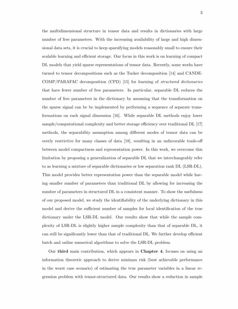
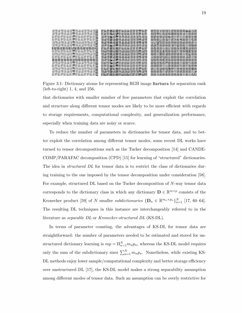
Figure 3.1: Dictionary atoms for representing RGB image Barbara for separation rank(left-to-right) 1, 4, and 256.

that dictionaries with smaller number of free parameters that exploit the correlation

and structure along different tensor modes are likely to be more efficient with regards

to storage requirements, computational complexity, and generalization performance,

especially when training data are noisy or scarce.

To reduce the number of parameters in dictionaries for tensor data, and to bet-

ter exploit the correlation among different tensor modes, some recent DL works have

turned to tensor decompositions such as the Tucker decomposition [14] and CANDE-

COMP/PARAFAC decomposition (CPD) [15] for learning of “structured” dictionaries.

The idea in structured DL for tensor data is to restrict the class of dictionaries dur-

ing training to the one imposed by the tensor decomposition under consideration [58].

For example, structured DL based on the Tucker decomposition of N -way tensor data

corresponds to the dictionary class in which any dictionary D ∈ Rm×p consists of the

Kronecker product [59] of N smaller subdictionaries Dn ∈ Rmn×pnNn=1 [17, 60–64].

The resulting DL techniques in this instance are interchangeably referred to in the

literature as separable DL or Kronecker-structured DL (KS-DL).

In terms of parameter counting, the advantages of KS-DL for tensor data are

straightforward: the number of parameters needed to be estimated and stored for un-

structured dictionary learning is mp = ΠNn=1mnpn, whereas the KS-DL model requires

only the sum of the subdictionary sizes∑N

n=1mnpn. Nonetheless, while existing KS-

DL methods enjoy lower sample/computational complexity and better storage efficiency

over unstructured DL [17], the KS-DL model makes a strong separability assumption

among different modes of tensor data. Such an assumption can be overly restrictive for

20

many classes of data [18], resulting in an unfavorable tradeoff between model compact-

ness and representation power.

Here, we overcome this limitation by proposing and studying a generalization of

KS-DL that we interchangeably refer to as learning a mixture of separable dictionaries

or low separation rank DL (LSR-DL). The separation rank of a matrix A is defined as

the minimum number of KS matrices whose sum equals A [65, 66]. The LSR-DL model

interpolates between the under-parameterized separable model (a special case of LSR-

DL model with separation rank 1) and the over-parameterized unstructured model.1

Figure 3.1 provides an illustrative example of the usefulness of LSR-DL, in which one

learns a dictionary with a small separation rank: while KS-DL learns dictionary atoms

that cannot reconstruct diagonal structures perfectly because of the abundance of hor-

izontal/vertical (DCT-like) structures within them, LSR-DL also returns dictionary

atoms with pronounced diagonal structures as the separation rank increases.2

3.1.1 Main Contributions

We first propose and analyze a generalization of the separable DL model—which we

call a mixture of separable dictionaries model or LSR-DL model—that allows for better

representation power than the separable model while having smaller number of param-

eters than standard DL. Our analysis assumes a generative model involving a true LSR

dictionary for tensor data and investigates conditions under which the true dictionary

is recoverable, up to a prescribed error, from training tensor data. Our first major

set of LSR dictionary identifiability results are for the conventional optimization-based

formulation of the DL problem [9], except that the search space is constrained to the

class of dictionaries with maximum separation rank r (and individual mixture terms

1While KS-DL corresponds to Tucker decompostition, its generalization LSR-DL does not correspondto any of the well-known tensor factorizations.

2The results presented in this chapter have been published in Proceedings of 2017 IEEE Interna-tional Workshop on Computational Advances in Multi-Sensor Adaptive Processing [67], Proceedingsof 2019 IEEE International Symposium on Information Theory [68], and IEEE Transactions on SignalProcessing [69].

21

having bounded norms when N ≥ 3 and r ≥ 2).3 Similar to conventional DL problems,

this LSR-DL problem is nonconvex with multiple global minima. We therefore focus on

local identifiability guarantees, meaning that a search algorithm initialized close enough

to the true dictionary can recover that dictionary.4 To this end, under certain assump-

tions on the generative model, we show that Ω(r(∑N

n=1mnpn)p2ρ−2)

samples ensure

existence of a local minimum of the constrained LSR-DL problem for Nth-order tensor

data within a neighborhood of radius ρ around the true LSR dictionary.

Our initial local identifiability results are based on an analysis of a separation rank-

constrained optimization problem that exploits a connection between LSR (resp., KS)

matrices and low-rank (resp., rank-1) tensors. However, a result in tensor recovery

literature [70] implies that finding the separation rank of a matrix is NP-hard. Our

second main contribution is development and analysis of two different relaxations of

the LSR-DL problem that are computationally tractable in the sense that they do not

require explicit computation of the separation rank. The first formulation once again

exploits the connection between LSR matrices and low-rank tensors and uses a convex

regularizer to implicitly constrain the separation rank of the learned dictionary. The

second formulation enforces the LSR structure on the dictionary by explicitly writing

it as a summation of r KS matrices. Our analyses of the two relaxations once again

involve conditions under which the true LSR dictionary is locally recoverable from

training tensor data. We also provide extensive discussion in the sequel to compare and

contrast the three sets of identifiability results for LSR dictionaries.

Our third main contribution is development of practical computational algorithms,

which are based on the two relaxations of LSR-DL, for learning of an LSR dictionary

in both batch and online settings. We then use these algorithms for learning of LSR

dictionaries for both synthetic and real tensor data, which are afterward used in de-

noising and representation learning tasks. Numerical results obtained as part of these

efforts help validate the usefulness of LSR-DL and highlight the different strengths and

3While we also provide identifiability results for LSR dictionaries without requiring the boundednessassumption, those results are only asymptotic in nature; see Section 3.3 for details.

4This is due to our choice of distance metric, which is the Frobenius norm.

22

weaknesses of the two LSR-DL relaxations and the corresponding algorithms.

3.1.2 Relation to Prior Work

Tensor decompositions [71, 72] have emerged as one of the main sets of tools that help

avoid overparameterization of tensor data models in a variety of areas. These include

deep learning, collaborative filtering, multilinear subspace learning, source separation,

topic modeling, and many other works (see [73, 74] and references therein). But the use

of tensor decompositions for reducing the (model and sample) complexity of dictionaries

for tensor data has been addressed only recently.

There have been many works that provide theoretical analysis for the sample com-

plexity of the conventional DL problem [75–78]. Among these, Gribonval et al. [77]

focus on the local identifiability of the true dictionary underlying vectorized data using

Frobenius norm as the distance metric. Shakeri et al. [17] extended this analysis for

the sample complexity of the KS-DL problem for Nth-order tensor data. This analysis

relies on expanding the objective function in terms of subdictionaries and exploiting the

coordinate-wise Lipschitz continuity property of the objective function with respect to

each subdictionary [17]. While this approach ensures the identifiability of the subdic-

tionaries, it requires the dictionary coefficient vectors to follow the so-called separable

sparsity model [79] and does not extend to the LSR-DL problem. In contrast, we pro-

vide local identifiability sample complexity results for the LSR-DL problem and two

relaxations of it. Further, our identifiability results hold for coefficient vectors following

the random sparsity model and the separable sparsity model.

In terms of computational algorithms, several works have proposed methods for

learning KS dictionaries that rely on alternating minimization techniques to update

the subdictionaries [61, 63, 79]. Among other works, Hawe et al. [60] employ a Rieman-

nian conjugate gradient method combined with a nonmonotone line search for KS-DL.

While they present the algorithm only for matrix data, its extension to higher-order

tensor data is trivial. Schwab et al. [80] have also recently addressed the separable

DL problem for matrix data; their contributions include a computational algorithm

and global recovery guarantees. In terms of algorithms for LSR-DL, Dantas et al. [62]

23

proposed one of the first methods for matrix data that uses a convex regularizer to

impose LSR on the dictionary. One of our batch algorithms, named STARK [81], also

uses a convex regularizer for imposing LSR structure. In contrast to Dantas et al. [62],

however, STARK can be used to learn a dictionary from tensor data of any order.

The other batch algorithm we propose, named TeFDiL, learns subdictionaries of the

LSR dictionary by exploiting the connection to tensor recovery and using tensor CPD.

Recently, Dantas et al. [82] proposed an algorithm for learning an LSR dictionary for

tensor data in which the dictionary update stage is a projected gradient descent algo-

rithm that involves a CPD after every gradient step. In contrast, TeFDiL only requires

a single CPD at the end of each dictionary update stage. Finally, while there exist a

number of online algorithms for DL [57, 83, 84], the online algorithms developed in here

are the first ones that enable learning of structured (either KS or LSR) dictionaries.

3.2 Preliminaries and Problem Statement

Notation and Definitions: We use underlined bold upper-case (A), bold upper-

case (A), bold lower-case (a), and lower-case (a) letters to denote tensors, matrices,

vectors, and scalars, respectively. For any integer p, we define [p] , 1, 2, · · · , p. We

denote the j-th column of a matrix A by aj . For an m × p matrix A and an index

set J ⊆ [p], we denote the matrix constructed from the columns of A indexed by J as

AJ . We denote by (An)Nn=1 an N -tuple (A1, · · · ,AN ), while AnNn=1 represents the

set A1, · · · ,AN. We drop the range indicators if they are clear from the context.

Norms and inner products: We denote by ‖v‖p the `p norm of vector v, while we use

‖A‖2, ‖A‖F , and ‖A‖tr to denote the spectral, Frobenius, and trace (nuclear) norms of

matrix A, respectively. Moreover, ‖A‖2,∞ , maxj ‖aj‖2 is the max column norm and

‖A‖1,1 ,∑

j ‖aj‖1. We define the inner product of two tensors (or matrices) A and B

as 〈A,B〉 , 〈vec(A), vec(B)〉 where vec(·) is the vectorization operator. The Euclidean

distance between two tuples of the same size is defined as∥∥(An)Nn=1 − (Bn)Nn=1

∥∥F

,√∑Nn=1 ||An −Bn||2F .

Kronecker product: We denote by A ⊗ B ∈ Rm1m2×p1p2 the Kronecker product of

24

matrices A ∈ Rm1×p1 and B ∈ Rm2×p2 . We use⊗N

n=1 Ai , A1 ⊗A2 ⊗ · · · ⊗AN for

the Kronecker product of N matrices. We drop the range indicators when there is no

ambiguity. We call a matrix a (N -th order) Kronecker-structured (KS) matrix if it is a

Kronecker product of N ≥ 2 matrices.

Definitions for matrices: For a matrix D with unit `2-norm columns, we define

the cumulative coherence µs as µs , max|J |≤s maxj /∈J ‖DTJDj‖1. We say a matrix D

satisfies the s-restricted isometry property (s-RIP) with constant δs if for any v ∈ Rs

and any J ⊆ [p] with |J | ≤ s, we have (1− δs)‖v‖22 ≤ ‖DJv‖22 ≤ (1 + δs)‖v‖22.

Definitions for tensors: We briefly present required tensor definitions here: see

Kolda and Bader [71] for more details. The mode-n unfolding matrix of A is denoted

by A(n), where each column of A(n) consists of the vector formed by fixing all indices

of A except the one in the nth-order. We denote the outer product (tensor product) of

vectors by , while ×n denotes the mode-n product between a tensor and a matrix. An

N -way tensor is rank-1 if it can be written as outer product of N vectors: v1 · · · vN .

Throughout this chapter, by the rank of a tensor, rank(A), we mean the CP-rank of

A, the minimum number of rank-1 tensors that construct A as their sum. The CP

decomposition (CPD), decomposes a tensor into sum of its rank-1 tensor components.

The Tucker decomposition factorizes an N -way tensor A ∈ Rm1×m2×···×mN as A =

X ×1 D1 ×2 D2 ×3 · · · ×N DN , where X ∈ Rp1×p2×···×pN denotes the core tensor and

Dn ∈ Rmn×pn denote factor matrices along the n-th mode of A for n ∈ [N ].

Notations for functions and spaces: We denote the element-wise sign function by

sgn(·). For any function f(x), we define the difference ∆f(x1; x2) , f(x1) − f(x2).

We denote by Um×p the Euclidean unit sphere: Um×p , D ∈ Rm×p|‖D‖F = 1. We

also denote the Euclidean sphere with radius α by αUm×p. The oblique manifold in

Rm×p is the manifold of matrices with unit-norm columns: Dm×p , D ∈ Rm×p|∀j ∈

[p], dTj dj = 1. We drop the dimension subscripts and use only D when there is no

ambiguity. The covering number of a set A with respect to a norm ‖ · ‖∗, denoted by

N∗(A, ε), is the minimum number of balls of ∗-norm radius ε needed to cover A.

Dictionary Learning Setup: In dictionary learning (DL) for vector data, we

25

assume observations y ∈ Rm are generated according to the following model:

y = D0x0 + ε, (3.1)

where D0 ∈ Dm×p ⊂ Rm×p is the true underlying dictionary, x0 ∈ Rp is a randomly

generated sparse coefficient vector, and ε ∈ Rm is the underlying noise vector. The goal

in DL is to recover the true dictionary given the noisy observations Y , ylLl=1 that

are independent realizations of (3.1). The ideal objective is to solve the statistical risk

minimization problem

minD∈C

fP(D) , Ey∼P fy(D), (3.2)

where P is the underlying distribution of the observations, C ⊆ Dm×p is the dictionary

class, typically selected for vector data to be the same as the oblique manifold, and

fy(D) , infx∈Rp

1

2‖y −Dx‖22 + λ‖x‖1. (3.3)

However, since we have access to the distribution P only through noisy observations

drawn from this distribution, we resort to solving the following empirical risk minimiza-

tion problem as a proxy for Problem (3.2):

minD∈C

FY(D) ,1

L

∑L

l=1fyl(D). (3.4)

Dictionary Learning for Tensor Data: To represent tensor data, conventional

DL approaches vectorize tensor data samples and treat them as one-dimensional arrays.

One way to explicitly account for the tensor structure in data is to use the Kronecker-

structured DL (KS-DL) model, which is based on the Tucker decomposition of tensor

data. In the KS-DL model, we assume that observations Yl ∈ Rm1×···×mN are generated

according to

Yl = X0l ×1 D0

1 ×2 D02 ×3 · · · ×N D0

N + E l, (3.5)

26

where D0n ∈ Rmn×pnNn=1 are generating subdictionaries, and X0

l and E l are the coef-

ficient and noise tensors, respectively. Equivalently, the generating model (3.5) can be

stated for yl , vec(Yl) as:

yl =(D0N ⊗D0

N−1 ⊗ · · · ⊗D01

)x0l + εl, (3.6)

where x0l , vec(X0

l) and εl , vec(E l) [71]. This is the same as the unstructured model

yl = D0x0l + εl with the additional condition that the generating dictionary is a Kro-

necker product of N subdictionaries. As a result, in the KS-DL problem, the constraint

set in (3.4) becomes C = KNm,p, where KNm,p , D ∈ Dm×p|D =⊗N

n=1 Dn, Dn ∈

Rmn×pn is the set of KS matrices with unit-norm columns and m and p are vectors

containing mn’s and pn’s, respectively.5

In summary, the structure in tensor data is exploited in the KS-DL model by as-

suming the dictionary is “separable” into subdictionaries for each mode. However, as

discussed earlier, this separable model is rather restrictive. Instead, we generalize the

KS-DL model using the notion of separation rank.6

Definition 4. The separation rank RNm,p(·) of a matrix A ∈ RΠnmn×Πnpn is the mini-

mum number r of N th-order KS matrices Ak =⊗N

n=1 Akn such that A =

r∑k=1

⊗Nn=1 Ak

n,

where Akn ∈ Rmn×pn.

The KS-DL model corresponds to dictionaries with separation rank 1. We instead

propose the low separation rank (LSR) DL model in which the separation rank of

the underlying dictionary is relatively small so that 1 ≤ Rm,p(D0) minm, p. This

generalizes the KS-DL model to a generating dictionary of the form D0 =∑r

k=1[DkN ]0⊗

[DkN−1]0 ⊗ · · · ⊗ [Dk

1]0, where r is the separation rank of D0. Consequently, defining

KN,rm,p , D ∈ Dm×p|RNm,p(D) ≤ r, the empirical rank-constrained LSR-DL problem is

minD∈KN,rm,p

FY(D). (3.7)

5We have changed the indexing of subdictionaries for ease of notation.

6The term was introduced in [66] for N = 2 (see also [65]).

27

However, the analytical tools at our disposal require the constraint set in (3.7) to be

closed, which we show does not hold for KN,rm,p when N ≥ 3 and r ≥ 2. In that case,

we instead analyze (3.7) with KN,rm,p replaced by (i) closure of KN,rm,p and (ii) a certain

closed subset of KN,rm,p. We refer the reader to Section 3.3 for further discussion.

In our study of the LSR-DL model, which includes the KS-DL model as a spe-

cial case, we use a correspondence between KS matrices and rank-1 tensors, stated in

Lemma 2 below, which allows us to leverage techniques and results in the tensor recov-

ery literature to analyze the LSR-DL problem and develop tractable algorithms. (This

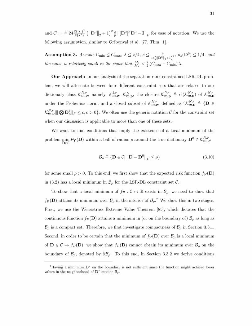
correspondence was first exploited in our earlier work [81].)

Lemma 2. Any N th-order Kronecker-structured matrix A = A1 ⊗A2 ⊗ · · · ⊗AN can

be rearranged as a rank-1, N th-order tensor Aπ = aN · · · a2 a1 with an , vec(An).

The proof of Lemma 2 (details of the rearrangement procedure) is provided in the

Appendix (Section 6.1). It follows immediately from Lemma 2 that if D =∑r

k=1 Dk1 ⊗

Dk2⊗· · ·⊗Dk

N , then we can rearrange matrix D into the tensor Dπ =∑r

k=1 dkN dkN−1

· · · dk1, where dkn = vec(Dkn). Therefore, we have the following equivalence:

RNm,p(D) ≤ r ⇐⇒ rank(Dπ) ≤ r.

This correspondence between separation rank and tensor rank highlights a challenge

with the LSR-DL problem: finding the rank of a tensor is NP-hard [70] and thus so is

finding the separation rank of a matrix. This makes Problem (3.7) in its current form

(and its variants) intractable. To overcome this, we introduce two tractable relaxations

to the rank-constrained Problem (3.7) that do not require explicit computation of the

tensor rank. The first relaxation uses a convex regularization term to implicitly impose

low tensor rank structure on Dπ, which results in a low separation rank D. The resulting

empirical regularization-based LSR-DL problem is

minD∈Dm×p

F regY (D) (3.8)

with F regY (D) , 1

L

∑Ll=1 fyl(D) + λ1g1(Dπ), where fy(D) is described in (3.3) and

28

g1(Dπ) is a convex regularizer to enforce low-rank structure on Dπ. The second re-

laxation is a factorization-based LSR-DL formulation in which the LSR dictionary is

explicitly written in terms of its subdictionaries. The resulting empirical risk minimiza-

tion problem is

minDk

n:∑rk=1

⊗Nn=1 Dk

n∈Dm×pF facY

(Dk

n), (3.9)

where F facY (Dk

n) , 1L

∑Ll=1 f

facyl

(Dkn) with

f facy (Dk

n) , infx∈Rp

∥∥∥y − (∑r

k=1

⊗N

n=1Dkn

)x∥∥∥2

+ λ ‖x‖1 ,

and the terms⊗N

n=1 Dkn are constrained as ‖

⊗Nn=1 Dk

n‖F ≤ c for some positive constant

c when N ≥ 3 and r ≥ 2.

In the rest of this chapter, we study the problem of identifying the true underly-

ing LSR-DL dictionary by analyzing the LSR-DL Problems (3.7)–(3.9) introduced in

this section and developing algorithms to solve Problems (3.8) and (3.9) in both batch

and online settings. Note that while Problem (3.7) (and its variants when N ≥ 3

and r ≥ 2) cannot be explicitly solved because of its NP-hardness, identifiability anal-

ysis of this problem—provided in Section 3.3—provides the basis for the analysis of

tractable Problems (3.8) and (3.9), provided in Section 3.4. To improve the readability

of our notation-heavy discussions and analysis, we have provided a table of notations

(Table 3.1) for easy access to definitions of the most commonly used notation.

3.3 Identifiability in the Rank-constrained LSR-DL Problem

In this section, we derive conditions under which a dictionary D0 ∈ KN,rm,p is identifiable

as a solution to either the separation rank-constrained problem in (3.7) or a slight

variant of (3.7) when N ≥ 3 and r ≥ 2. Specifically, we show that under certain

assumptions on the generative model, there is at least one local minimum D∗ of either

Problem (3.7) or one of its variants that is “close” to the underlying dictionary D0.

Notwithstanding the fact that no efficient algorithm exists to solve the intractable

29

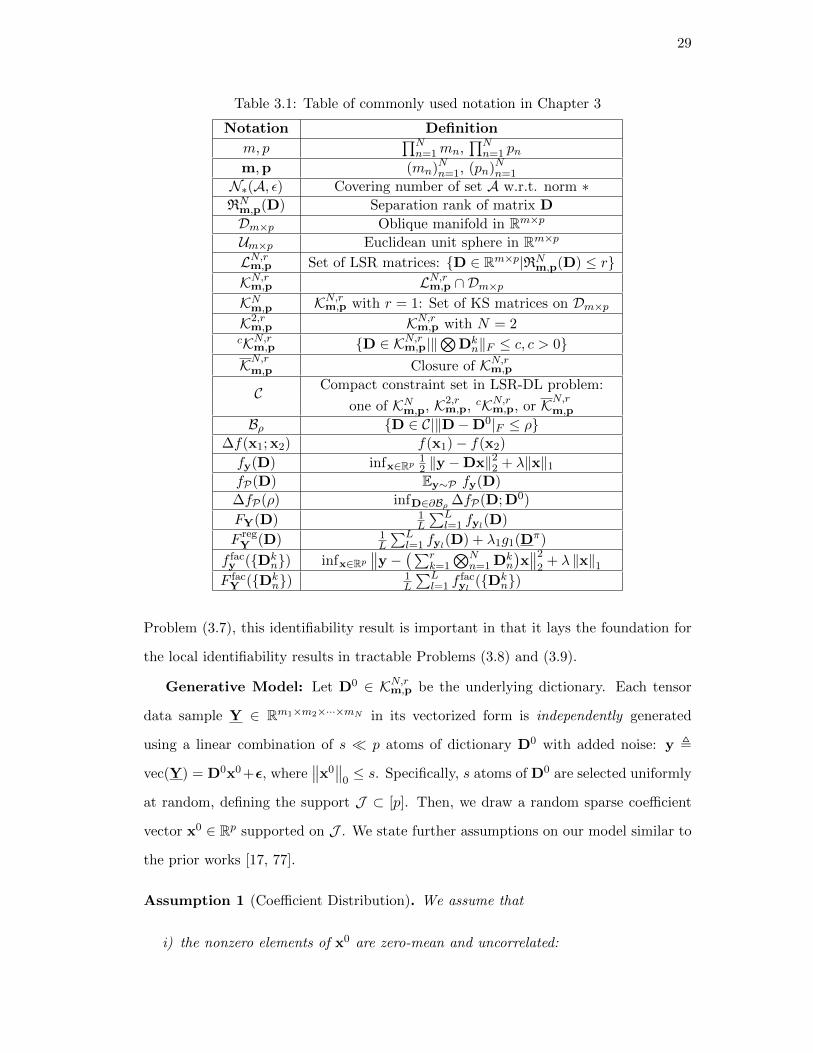
Table 3.1: Table of commonly used notation in Chapter 3

Notation Definition

m, p∏Nn=1mn,

∏Nn=1 pn

m,p (mn)Nn=1, (pn)Nn=1

N∗(A, ε) Covering number of set A w.r.t. norm ∗RN

m,p(D) Separation rank of matrix D

Dm×p Oblique manifold in Rm×pUm×p Euclidean unit sphere in Rm×p

LN,rm,p Set of LSR matrices: D ∈ Rm×p|RNm,p(D) ≤ r

KN,rm,p LN,rm,p ∩ Dm×pKNm,p KN,rm,p with r = 1: Set of KS matrices on Dm×pK2,r

m,p KN,rm,p with N = 2cKN,rm,p D ∈ KN,rm,p|‖

⊗Dkn‖F ≤ c, c > 0

KN,rm,p Closure of KN,rm,p

C Compact constraint set in LSR-DL problem:

one of KNm,p, K2,rm,p, cKN,rm,p, or KN,rm,p

Bρ D ∈ C|‖D−D0|F ≤ ρ∆f(x1; x2) f(x1)− f(x2)

fy(D) infx∈Rp12 ‖y −Dx‖22 + λ‖x‖1

fP(D) Ey∼P fy(D)

∆fP(ρ) infD∈∂Bρ ∆fP(D; D0)

FY(D) 1L

∑Ll=1 fyl(D)

F regY (D) 1

L

∑Ll=1 fyl(D) + λ1g1(Dπ)

f facy (Dk

n) infx∈Rp∥∥y − (∑r

k=1

⊗Nn=1 Dk

n

)x∥∥2

2+ λ ‖x‖1

F facY (Dk

n) 1L

∑Ll=1 f

facyl

(Dkn)

Problem (3.7), this identifiability result is important in that it lays the foundation for

the local identifiability results in tractable Problems (3.8) and (3.9).

Generative Model: Let D0 ∈ KN,rm,p be the underlying dictionary. Each tensor

data sample Y ∈ Rm1×m2×···×mN in its vectorized form is independently generated

using a linear combination of s p atoms of dictionary D0 with added noise: y ,

vec(Y) = D0x0 +ε, where∥∥x0

∥∥0≤ s. Specifically, s atoms of D0 are selected uniformly

at random, defining the support J ⊂ [p]. Then, we draw a random sparse coefficient

vector x0 ∈ Rp supported on J . We state further assumptions on our model similar to

the prior works [17, 77].

Assumption 1 (Coefficient Distribution). We assume that

i) the nonzero elements of x0 are zero-mean and uncorrelated:

30

Ex0J [x0

J ]T |J

= Ex2 · Is,

ii) the nonzero elements of s0 , sgn(x0) are zero-mean and uncorrelated:

Es0J [s0J ]T |J

= Is,

iii) x0 and s0 are uncorrelated: Es0J [x0

J ]T |J

= E|x| · Is,

iv) x0 has bounded norm almost surely:∥∥x0

∥∥2≤Mx with probability 1,

v) nonzero elements of x0 are far from zero almost surely: minj∈J|x0j | ≥ x with proba-

bility 1.

Assumption 2 (Noise Distribution). We make the following assumptions on the dis-

tribution of the noise ε:

i) the elements of ε are zero-mean and uncorrelated: EεεT |J

= Eε2 · I,

ii) ε is uncorrelated with x0 and s0: Ex0εT |J

= E

s0εT |J

= 0,

iii) ε has bounded norm almost surely: ‖ε‖2 ≤Mε with probability 1.

Note that Assumptions 1-iv and 2-iii imply the magnitude of y is bounded: ‖y‖2 ≤

My. Next, we define positive parameters λ , λE|x| , Cmax , 2E|x|

7Mx

(1− 2µs(D

0)),

Figure 3.2: Example of rearranging a Kronecker structured matrix (N = 3) into a thirdorder rank-1 tensor.

31

and Cmin , 24E|x|2Ex2

(∥∥D0∥∥

2+ 1)2 s

p

∥∥[D0]TD0 − I∥∥F

for ease of notation. We use the

following assumption, similar to Gribonval et al. [77, Thm. 1].

Assumption 3. Assume Cmin ≤ Cmax, λ ≤ x/4, s ≤ p

16(‖D0‖2+1)2 , µs(D

0) ≤ 1/4, and

the noise is relatively small in the sense that MεMx

< 72 (Cmax − Cmin) λ.

Our Approach: In our analysis of the separation rank-constrained LSR-DL prob-

lem, we will alternate between four different constraint sets that are related to our

dictionary class KN,rm,p, namely, K2,rm,p, KNm,p, the closure KN,rm,p , cl(KN,rm,p) of KN,rm,p

under the Frobenius norm, and a closed subset of KN,rm,p, defined as cKN,rm,p , D ∈

KN,rm,p|‖⊗

Dkn‖F ≤ c, c > 0. We often use the generic notation C for the constraint set

when our discussion is applicable to more than one of these sets.

We want to find conditions that imply the existence of a local minimum of the

problem minD∈C

FY(D) within a ball of radius ρ around the true dictionary D0 ∈ KN,rm,p:

Bρ , D ∈ C|∥∥D−D0

∥∥F≤ ρ (3.10)

for some small ρ > 0. To this end, we first show that the expected risk function fP(D)

in (3.2) has a local minimum in Bρ for the LSR-DL constraint set C.

To show that a local minimum of fP : C 7→ R exists in Bρ, we need to show that

fP(D) attains its minimum over Bρ in the interior of Bρ.7 We show this in two stages.

First, we use the Weierstrass Extreme Value Theorem [85], which dictates that the

continuous function fP(D) attains a minimum in (or on the boundary of) Bρ as long as

Bρ is a compact set. Therefore, we first investigate compactness of Bρ in Section 3.3.1.

Second, in order to be certain that the minimum of fP(D) over Bρ is a local minimum

of D ∈ C 7→ fP(D), we show that fP(D) cannot obtain its minimum over Bρ on the

boundary of Bρ, denoted by ∂Bρ. To this end, in Section 3.3.2 we derive conditions

7Having a minimum D∗ on the boundary is not sufficient since the function might achieve lowervalues in the neighborhood of D∗ outside Bρ.

32

that if ∂Bρ is nonempty then8

∆fP(ρ) , infD∈∂Bρ

∆fP(D; D0) > 0, (3.11)

which implies fP(D) cannot achieve its minimum on ∂Bρ.

Finally, in Section 3.3.3 we use concentration of measure inequalities to relate FY(D)

in (3.4) to fP(D) and find the number of samples needed to guarantee (with high

probability) that FY(D) also has a local minimum in the interior of Bρ.

3.3.1 Compactness of the Constraint Sets

When the constraint set C is a compact subset of the Euclidean space Rm×p, the subset

Bρ is also compact. Thus, we first investigate the compactness of the constraint set

KN,rm,p. Since KN,rm,p is a bounded set, according to the Heine-Borel Theorem [85], it is

a compact subset of Rm×p if and only if it is closed. Also, KN,rm,p can be written as

the intersection of LN,rm,p , D ∈ Rm×p|RNm,p(D) ≤ r and the oblique manifold D. In

order for KN,rm,p = LN,rm,p∩D to be closed, it suffices to show that LN,rm,p and D are closed.

It is trivial to show D is closed; hence, we focus on whether LN,rm,p is closed.

In the following, we use the facts that the constraint RNm,p(D) ≤ r is equivalent

to rank(Dπ) ≤ r and that the rearrangement mapping that sends D to Dπ preserves

topological properties of sets such as the distances between the set elements under the

Frobenius norm. These facts allow us to translate the topological properties of tensor

sets into properties of the structured matrices that we study here.

Lemma 3. Let N ≥ 3 and r ≥ 2. Then, the set LN,rm,p is not closed. However, the set

of KS matrices LN,1m,p and the set L2,rm,p are closed.

Proof. Proposition 4.1 in De Silva and Lim [86] shows that the space of tensors of order

N ≥ 3 and rank r ≥ 2 is not closed. The fact that the rearrangement process preserves

topological properties of sets means that the same result holds for the set LN,rm,p with

N ≥ 3 and rank r ≥ 2.

8If the boundary is empty, it is trivial that the infimum is attained in the interior of the set.

33

The proof for closedness of LN,1m,p and L2,rm,p follows from Propositions 4.2 and 4.3 in

De Silva and Lim [86], which can be adopted here due to the relation between the sets

of low-rank tensors and LSR matrices.

To illustrate the non-closedness of LN,rm,p for N ≥ 3 and r ≥ 2 and motivate the

use of the sets KN,rm,p and cKN,rm,p in lieu of KN,rm,p, we provide an example. Consider the

sequence Dt := t(A1 + 1

tB1

)⊗(A2 + 1

tB2

)⊗(A3 + 1

tB3

)) − tA1 ⊗ A2 ⊗ A3 where

Ai,Bi ∈ Rmi×pi are linearly independent pairs. It is clear that R3m,p(Dt) ≤ 2 for any

t. The limit point of this sequence, however, is limt→∞Dt = A1 ⊗ A2 ⊗ B3 + A1 ⊗

B2⊗A3 + B1⊗A2⊗B3, which is a separation-rank-3 matrix. Therefore, the set L3,2m,p

is not closed.

The non-closedness of LN,rm,p means there exist sequences in LN,rm,p whose limit points

are not in the set. Two possible solutions to circumvent this issue include: (i) use the

closure of LN,rm,p as the constraint set, and (ii) eliminate such sequences from LN,rm,p. We

discuss each solution in detail below.

Adding the limit points

We denote the closure of LN,rm,p by LN,rm,p , cl(LN,rm,p). By slightly relaxing the constraint

set in (3.7) to LN,rm,p ∩ D, we can instead solve the following:

minD∈KN,rm,p

FY(D), (3.12)

where KN,rm,p = LN,rm,p ∩ D. Note that (i) a solution to (3.7) is a solution to (3.12) and

(ii) a solution to (3.12) is either a solution to (3.7) or is arbitrarily close to a member

of KN,rm,p.9

9The first argument holds since if FY(D∗) ≤ FY(D) for all D ∈ KN,rm,p, by continuity it also holds

for all D ∈ KN,rm,p. The second argument is trivial.

34

Eliminating the problematic sequences

In order to exclude the sequences Dt → D such that Dt ∈ LN,rm,p for all t and D /∈ LN,rm,p,

we first need to characterize them.

Lemma 4. Assume Dt → D where RNm,p(Dt) ≤ r and RN

m,p(D) > r. We can write

Dt =∑r

k=1 λkt

⊗Nn=1[Dk

n]t where∥∥[Dk

n]t∥∥F

= 1. Then, maxk |λkt | → ∞ as t → ∞. In

fact, at least two of the coefficient sequences λkt are unbounded.

Proof. The rearrangement process allows us to borrow the results in Proposition 4.8 in

De Silva and Lim [86] for tensors and apply them to LSR matrices.

The following corollary of Lemma 4 suggests that one can exclude the problematic

sequences from LN,rm,p by bounding the norm of individual KS (separation-rank-1) terms.

Corollary 1. Consider the set LN,rm,p whose members can be written as D =r∑

k=1

N⊗n=1

Dkn

such that Dkn ∈ Rmn×pn. Then, for any c > 0 the set cLN,rm,p =

D ∈ LN,rm,p|

∥∥⊗Dkn

∥∥F≤

c

is closed.

We have now shown that the sets K2,rm,p, KNm,p , KN,1m,p, cKN,rm,p = cLN,rm,p ∩ D, and

KN,rm,p = LN,rm,p ∩ D are compact subsets of Rm×p. Next, we provide asymptotic identifi-

ability results for these compact constraint sets.

3.3.2 Asymptotic Analysis for Dictionary Identifiability

Now that we have discussed the compactness of the relevant constraint sets, we are

ready to show that the minimum of fy(D) over Bρ, defined in (3.10), is not attained on

∂Bρ. This will complete our proof of existence of a local minimum of fP(D) in Bρ. In

our proof, we make use of a result in Gribonval et al. [77], presented here in Lemma 5.

Lemma 5 (Theorem 1 in Gribonval et al. [77]). Consider the statistical DL Problem

(3.2) with constraint set D. Suppose the generating dictionary D0 ∈ D and Assumptions

1–3 hold. Then, for any ρ such that λCmin < ρ ≤ λCmax and MεMx

< 72(λCmax − ρ), we

35

have

∆fP(ρ) ≥ Ex28· sp· ρ(ρ− λCmin

)> 0. (3.13)

for all D ∈ D such that ‖D−D0‖F = ρ.

Interested readers can find the detailed proof of Lemma 5 in Gribonval et al. [77].

The following theorem states our first identifiability result for the LSR-DL model.

Theorem 4. Consider the statistical DL Problem (3.2) with constraint set C being

either K2,rm,p, KNm,p, cKN,rm,p or KN,rm,p. Suppose the generating dictionary D0 ∈ C and

Assumptions 1–3 hold. Then, for any ρ such that λCmin < ρ < λCmax and MεMx

<

72(λCmax − ρ), the function D ∈ C 7→ fP(D) has a local minimum D∗ such that∥∥D∗ −D0

∥∥F< ρ.

Proof. Since fP(D) is a continuous function and the ball Bρ = D ∈ C|∥∥D−D0

∥∥F≤

ρ is compact, by the extreme value theorem, D ∈ Bρ 7→ fP(D) attains its infimum at

a point in the ball. If this minimum is attained in the interior of Bρ then it is a local

minimum of D ∈ C 7→ fP(D). Therefore, a key ingredient of the proof is showing that

fP(D) > fP(D0) for all D ∈ ∂Bρ if ∂Bρ is nonempty. Lemma 5 states the conditions

under which fP(D) > fP(D0) on ∂Sρ, where Sρ ,D ∈ D

∣∣ ∥∥D−D0∥∥F≤ ρ

.

Since ∂Bρ ⊂ ∂Sρ, the result of Lemma 5 can be used for our problem as well, i.e.

for any D ∈ ∂Bρ, we have fP(D) > fP(D0), when Cminλ < ρ < Cmaxλ. It follows from

this result together with the existence of the infimum of fP(D) : Bρ 7→ R in Bρ that

Problem (3.2) has a local minimum within a ball of radius ρ around the true dictionary

D0.

Next, we discuss finite sample identifiability of the true dictionary D0 for three of

the constraint sets.

3.3.3 Sample Complexity for Dictionary Identifiability

We now derive the number of samples required to guarantee, with high probability,

that FY : C 7→ R has a local minimum at a point “close” to D0 when the constraint set

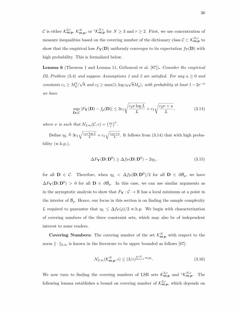
36

C is either K2,rm,p, KNm,p, or cKN,rm,p for N ≥ 3 and r ≥ 2. First, we use concentration of

measure inequalities based on the covering number of the dictionary class C ⊂ KN,rm,p to

show that the empirical loss FY(D) uniformly converges to its expectation fP(D) with

high probability. This is formalized below.

Lemma 6 (Theorem 1 and Lemma 11, Gribonval et al. [87]). Consider the empirical

DL Problem (3.4) and suppose Assumptions 1 and 2 are satisfied. For any u ≥ 0 and

constants c1 ≥M2y /√

8 and c2 ≥ max(1, log c0

√8My), with probability at least 1− 2e−u

we have

supD∈C|FY(D)− fp(D)| ≤ 3c1

√c2ν logL

L+ c1

√c2ν + u

L, (3.14)

where ν is such that N2,∞(C, ε) =(c0ε

)ν.

Define ηL , 3c1

√c2ν logL

L + c1

√c2ν+uL . It follows from (3.14) that with high proba-

bility (w.h.p.),

∆FY(D; D0) ≥ ∆fP(D; D0)− 2ηL, (3.15)

for all D ∈ C. Therefore, when ηL < ∆fP(D; D0)/2 for all D ∈ ∂Bρ, we have

∆FY(D; D0) > 0 for all D ∈ ∂Bρ. In this case, we can use similar arguments as

in the asymptotic analysis to show that FY : C → R has a local minimum at a point in

the interior of Bρ. Hence, our focus in this section is on finding the sample complexity

L required to guarantee that ηL ≤ ∆fP(ρ)/2 w.h.p. We begin with characterization

of covering numbers of the three constraint sets, which may also be of independent

interest to some readers.

Covering Numbers: The covering number of the set KNm,p with respect to the

norm ‖ · ‖2,∞ is known in the literature to be upper bounded as follows [87]:

N2,∞(KNm,p, ε) ≤ (3/ε)∑Ni=1 mipi . (3.16)

We now turn to finding the covering numbers of LSR sets K2,rm,p and cKN,rm,p. The

following lemma establishes a bound on covering number of K2,rm,p, which depends on

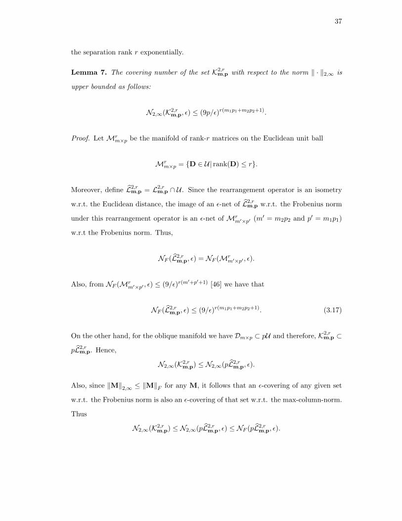
37

the separation rank r exponentially.

Lemma 7. The covering number of the set K2,rm,p with respect to the norm ‖ · ‖2,∞ is

upper bounded as follows:

N2,∞(K2,rm,p, ε) ≤ (9p/ε)r(m1p1+m2p2+1).

Proof. Let Mrm×p be the manifold of rank-r matrices on the Euclidean unit ball

Mrm×p = D ∈ U| rank(D) ≤ r.

Moreover, define L2,rm,p = L2,r

m,p ∩ U . Since the rearrangement operator is an isometry

w.r.t. the Euclidean distance, the image of an ε-net of L2,rm,p w.r.t. the Frobenius norm

under this rearrangement operator is an ε-net of Mrm′×p′ (m′ = m2p2 and p′ = m1p1)

w.r.t the Frobenius norm. Thus,

NF (L2,rm,p, ε) = NF (Mr

m′×p′ , ε).

Also, from NF (Mrm′×p′ , ε) ≤ (9/ε)r(m

′+p′+1) [46] we have that

NF (L2,rm,p, ε) ≤ (9/ε)r(m1p1+m2p2+1). (3.17)

On the other hand, for the oblique manifold we have Dm×p ⊂ pU and therefore, K2,rm,p ⊂

pL2,rm,p. Hence,

N2,∞(K2,rm,p) ≤ N2,∞(pL2,r

m,p, ε).

Also, since ‖M‖2,∞ ≤ ‖M‖F for any M, it follows that an ε-covering of any given set

w.r.t. the Frobenius norm is also an ε-covering of that set w.r.t. the max-column-norm.

Thus

N2,∞(K2,rm,p) ≤ N2,∞(pL2,r

m,p, ε) ≤ NF (pL2,rm,p, ε).

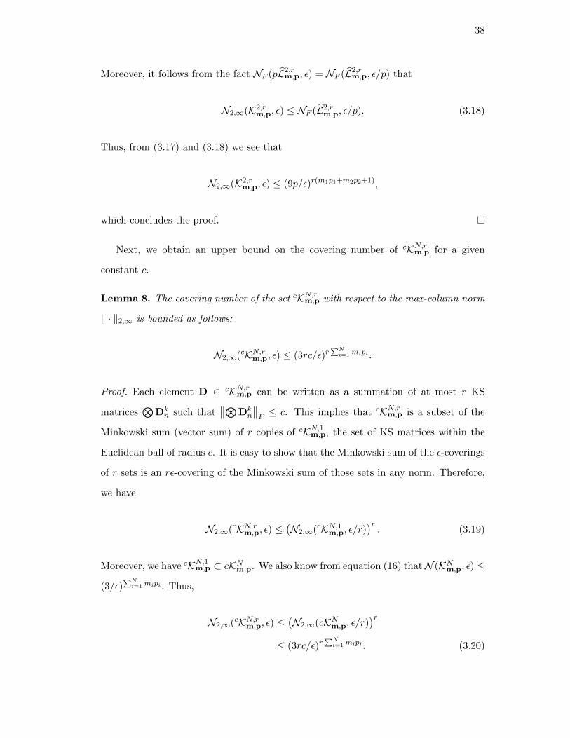
38

Moreover, it follows from the fact NF (pL2,rm,p, ε) = NF (L2,r

m,p, ε/p) that

N2,∞(K2,rm,p, ε) ≤ NF (L2,r

m,p, ε/p). (3.18)

Thus, from (3.17) and (3.18) we see that

N2,∞(K2,rm,p, ε) ≤ (9p/ε)r(m1p1+m2p2+1),

which concludes the proof.

Next, we obtain an upper bound on the covering number of cKN,rm,p for a given

constant c.

Lemma 8. The covering number of the set cKN,rm,p with respect to the max-column norm

‖ · ‖2,∞ is bounded as follows:

N2,∞(cKN,rm,p, ε) ≤ (3rc/ε)r∑Ni=1mipi .

Proof. Each element D ∈ cKN,rm,p can be written as a summation of at most r KS

matrices⊗

Dkn such that

∥∥⊗Dkn

∥∥F≤ c. This implies that cKN,rm,p is a subset of the

Minkowski sum (vector sum) of r copies of cKN,1m,p, the set of KS matrices within the

Euclidean ball of radius c. It is easy to show that the Minkowski sum of the ε-coverings

of r sets is an rε-covering of the Minkowski sum of those sets in any norm. Therefore,

we have

N2,∞(cKN,rm,p, ε) ≤(N2,∞(cKN,1m,p, ε/r)

)r. (3.19)

Moreover, we have cKN,1m,p ⊂ cKNm,p. We also know from equation (16) thatN (KNm,p, ε) ≤

(3/ε)∑Ni=1 mipi . Thus,

N2,∞(cKN,rm,p, ε) ≤(N2,∞(cKNm,p, ε/r)

)r≤ (3rc/ε)r

∑Ni=1 mipi . (3.20)

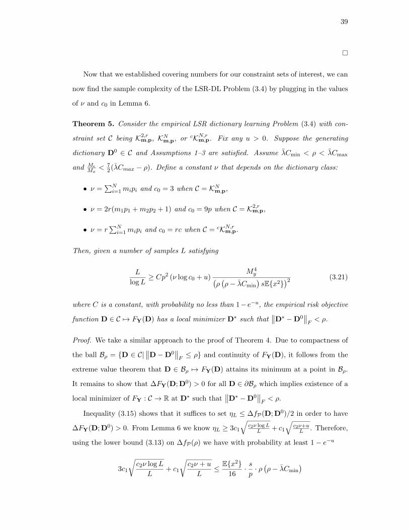
39

Now that we established covering numbers for our constraint sets of interest, we can

now find the sample complexity of the LSR-DL Problem (3.4) by plugging in the values

of ν and c0 in Lemma 6.

Theorem 5. Consider the empirical LSR dictionary learning Problem (3.4) with con-

straint set C being K2,rm,p, KNm,p, or cKN,rm,p. Fix any u > 0. Suppose the generating

dictionary D0 ∈ C and Assumptions 1–3 are satisfied. Assume λCmin < ρ < λCmax

and MεMx

< 72(λCmax − ρ). Define a constant ν that depends on the dictionary class:

• ν =∑N

i=1mipi and c0 = 3 when C = KNm,p,

• ν = 2r(m1p1 +m2p2 + 1) and c0 = 9p when C = K2,rm,p,

• ν = r∑N

i=1mipi and c0 = rc when C = cKN,rm,p.

Then, given a number of samples L satisfying

L

logL≥ Cp2 (ν log c0 + u)

M4y(

ρ(ρ− λCmin

)sEx2

)2 (3.21)

where C is a constant, with probability no less than 1− e−u, the empirical risk objective

function D ∈ C 7→ FY(D) has a local minimizer D∗ such that∥∥D∗ −D0

∥∥F< ρ.

Proof. We take a similar approach to the proof of Theorem 4. Due to compactness of

the ball Bρ = D ∈ C|∥∥D−D0

∥∥F≤ ρ and continuity of FY(D), it follows from the

extreme value theorem that D ∈ Bρ 7→ FY(D) attains its minimum at a point in Bρ.

It remains to show that ∆FY(D; D0) > 0 for all D ∈ ∂Bρ which implies existence of a

local minimizer of FY : C → R at D∗ such that∥∥D∗ −D0

∥∥F< ρ.

Inequality (3.15) shows that it suffices to set ηL ≤ ∆fP(D; D0)/2 in order to have

∆FY(D; D0) > 0. From Lemma 6 we know ηL ≥ 3c1

√c2ν logL

L + c1

√c2ν+uL . Therefore,

using the lower bound (3.13) on ∆fP(ρ) we have with probability at least 1− e−u

3c1

√c2ν logL

L+ c1

√c2ν + u

L≤ Ex2

16· sp· ρ(ρ− λCmin

)

40

with c1 ≥M2y /√

8 and c2 ≥ max(1, log c0

√8My)

10. Rearranging, we get

L

logL≥ c2

1

(3√c2ν +

√c2ν + u

ρ(ρ− λCmin

) )2(16

Ex2· ps

)2

. (3.22)

Setting c1 ≥M2y /√

8 and c2 = c3 log c0 ≥ max(1, log c0

√8My) we get the lower bound

L

logL≥ Cp2 (ν log c0 + u)

(M2y

ρ(ρ− λCmin

)sEx2

)2

with probability at least 1 − e−u. Given that the number of samples satisfies (3.21)

for λCmin < ρ < λCmax, with high probability ∆FY > 0 for any D ∈ ∂Bρ. Therefore,

it follows from the existence of the infimum of D ∈ Bρ 7→ FY(D) in Bρ that D ∈

C 7→ FY(D) has a local minimum at a point within a ball of radius ρ around the true

dictionary D0.

The Ω(r(∑

nmnpn)p2ρ−2)

sample complexity we obtain here for rank-constrained

LSR-DL is a reduction compared to the Ω(mp3ρ−2) sample complexity of standard DL

in [77]. However, a minimax lower bound scaling of Ω(p∑

nmnpnρ−2) in [64] for KS-DL

(r = 1) suggests an O(p) gap with our upper bound.

3.4 Identifiability in the Tractable LSR-DL Problems

In Section 3.2, we introduced two tractable relaxations to the rank-constrained LSR-

DL problem: a regularized problem (3.8) with a convex regularization term and a

factorization-based problem (3.9) in which the dictionary is written in terms of its

subdictionaries. Based on our results in Section 3.3 for the rank-constrained problem,

we now provide results on the local identifiability of the true dictionary D0 in these

problems, i.e., we find conditions under which at least one local minimizer of these

problems is located near the true dictionary D0. Such local identifiability result implies

that any DL algorithm that converges to a local minimum of these problems can recover

10Under the conditions of this theorem, My ≤√

1 + δs(D0)Mx +Mε, where δs(D0) denotes the RIP

constant of D0.

41

D0 up to a small error if it is initialized close enough to D0.

3.4.1 Regularization-based LSR Dictionary Learning

The first tractable LSR-DL problem that we study is the regularized problem (3.8).

Exploiting the relation between RNm,p(D) and rank(Dπ), the LSR structure is enforced

on the dictionary by a convex regularizer that imposes low tensor rank structure on

Dπ. The regularizer that we use here is a commonly used convex proxy for the tensor

rank function, the sum-trace-norm [88], which is defined as the average of the trace

(nuclear) norms of the unfoldings of the tensor: ‖A‖str ,∑N

n=1

∥∥A(n)∥∥

tr.

The first question we address is whether the reference dictionary that generates the

observations YlLl=1 is identifiable via Problem (3.8). Our local identifiability result

here is limited to when D0 ∈ KNm,p, i.e. the true dictionary is KS. For such D0, we

show that there is at least one local minimizer D∗ of F regY (D) under Assumptions 1–3

that is close to D0.

Theorem 6. Consider the regularized LSR-DL problem (3.8). Suppose that the gener-

ating dictionary D0 ∈ KNm,p and Assumptions 1–3 are satisfied. Moreover, let λCmin <

ρ ≤ λCmax and MεMx

< 72(λCmax − ρ). Then, the expected risk function D ∈ D 7→

E[F regY (D)] has a local minimizer D∗ such that

∥∥D∗ −D0∥∥F≤ ρ.

Moreover, given L samples such that

L > C0p2(mp+ u)

(M2x

Ex2·MεMx

+ ρ+ (MεMx

+ ρ)2

ρ− Cminλ

)2

, (3.23)

where u and C are positive constants, then, we have with probability no less than 1−e−u

that the empirical risk function D ∈ D 7→ F regY (D) has a local minimum at D∗ such

that∥∥D∗ −D0

∥∥F< ρ.

Proof. Consider the ball Bρ = D ∈ D|∥∥D−D0

∥∥F≤ ρ. It follows from the extreme

value theorem [85] that D ∈ Bρ 7→ F regY (D) attains its minimum at a point in Bρ. This

is based on compactness of Bρ = D ∈ C|∥∥D−D0

∥∥F≤ ρ and continuity of F reg

Y (D).

Similarly, D ∈ Bρ 7→ f regP (D) , E[F reg

Y ] reaches its minimum at a point in Bρ. We now

42

need to show in either case the minimum is not attained on the boundary of Bρ. To

this end, we show in the following that ∆F regY (D; D0) > 0 and ∆f reg

P (D; D0) > 0 for

any D ∈ ∂Bρ.

Incorporation of the trace-norm regularization term in (3.8) whithin the objective

in (3.4) introduces a factor ‖Dπ‖str −∥∥[D0]π

∥∥str

=∑N

n=1

(∥∥D(n)∥∥

tr−∥∥[D0](n)

∥∥tr

)to

∆fP(D; D0) and ∆FY(D; D0). We know from Lemma 2 that when the true dictionary

is a KS matrix (D0 ∈ KNm,p), its rearrangement tensor [D0]π is a rank-1 tensor and

therefore all unfoldings [D0](n) of [D0]π are rank-1 matrices. This implies ‖D(n)‖tr =

‖D(n)‖F . Likewise, for all D ∈ Dm×p we have∥∥D(n)

∥∥F

=∥∥[D0](n)

∥∥F

=√p. Therefore,

∥∥D(n)∥∥

tr−∥∥[D0](n)

∥∥tr

=∑rn

k=1σk(D

(n))−√p

≥√∑rn

k=1σ2k(D

(n))−√p = 0,

where rn , rank(D(n)) and σk(D(n)) denotes the k-th singular value of D(n). Therefore,

we conclude that ∆F regY (D; D0) ≥ ∆FY(D; D0) and ∆f reg

P (D; D0) ≥ ∆fP(D; D0) for

any D ∈ D. According to Lemma 5, ∆fP(D; D0) > 0 for all D on the boundary of the

ball Bρ. Furthermore, under the assumptions of the current theorem, given a number

of samples satisfying (3.23), Gribonval et al. [77] show that the empirical difference

∆FY(D; D0) > 0 for all D on the boundary of Sρ =D ∈ D

∣∣ ∥∥D−D0∥∥F≤ ρ

, and

therefore on the boundary of Bρ ⊆ Sρ, with probability at least 1− e−u. Therefore, for

both f regP (D) and F reg

Y (D), the minimum is attained in the interior of Bρ and not on

its boundary.

3.4.2 Factorization-based LSR Dictionary Learning

We now shift our focus to Problem (3.9), which expands D as∑r

k=1

⊗Dkn and optimizes

over the individual subdictionaries, and show that there is at least one local minimum

[Dkn]∗ of the factorization-based LSR-DL Problem (3.9) such that

∑⊗[Dk

n]∗ is close

to the underlying dictionary D0. Our strategy here is to establish a connection between

the local minima of (3.9) and those of (3.4). Specifically, we show that when the

dictionary class in (3.7) matches that of (3.9), for every local minimum D of (3.4),

43

there exists a local minimum Dkn of (3.9) such that D =

∑⊗Dkn. Furthermore, we

use the result of Theorems 4 and 5 that there exists a local minimum D∗ of Problem

(3.4) within a small ball around D0. It follows from these facts that under the generating

model considered here, a local minimum [Dkn]∗ of (3.9) is such that

∑⊗[Dk

n]∗ is close

to D0.

We begin with a bound on the distance between LSR matrices when the tuples of

their factor matrices are ε-close.

Lemma 9. For any two tuples (Akn) and (Bk

n) such that Akn,B

kn ∈ αUmn×pn for

all n ∈ [N ] and k ∈ [r], if the distance∥∥(Ak

n) − (Bkn)∥∥F≤ ε then

∥∥∑rk=1

⊗Akn −∑r

k=1

⊗Bkn

∥∥F≤ αN−1

√Nrε.

Proof. According to Lemma 2 in Shakeri et al. [17], for any An and Bn we have

⊗N

n=1An −

⊗N

n=1Bn

=∑N

n=1Γ1 ⊗ · · · ⊗ (An −Bn)⊗ · · · ⊗ ΓN , (3.24)

where Γn = An or Γn = Bn depending on n. Let εkn , ‖Akn − Bk

n‖F . Using equality

(3.24), we have

∥∥∑r

k=1

⊗Akn −

∑r

k=1

⊗Bkn

∥∥F

=∥∥ r∑k=1

N∑n=1

Γk1 ⊗ · · · ⊗ (Akn −Bk

n)⊗ · · · ⊗ ΓkN∥∥F

≤r∑

k=1

N∑n=1

∥∥Γk1 ⊗ · · · ⊗ (Akn −Bk

n)⊗ · · · ⊗ ΓkN∥∥F

= αN−1r∑

k=1

N∑n=1

εkn(a)

≤ αN−1√Nrε, (3.25)

where the inequality (a) follows from ‖(εkn)‖1 ≤√Nr ‖(εkn)‖2 ≤

√Nrε.

Theorem 7. Consider the factorization-based LSR-DL problem (3.9). Suppose that

Assumptions 1–3 are satisfied and MεMx

< 72(λCmax − ρ) with λCmin < ρ ≤ λCmax.

Then, the expected risk function E[F facY

(Dk

n)] has a local minimizer ([Dk

n]∗) such that

44

∥∥∑⊗[Dk

n]∗ −D0∥∥F≤ ρ.

Moreover, when the sample complexity requirements (3.21) are satisfied for some

positive constant u, then with probability no less than 1−e−u the empirical risk function

F facY

(Dk

n)

has a local minimum achieved at ([Dkn]∗) such that

∥∥∑⊗[Dk

n]∗ −D0∥∥F≤

ρ.

Proof. Let us first consider the finite sample case. Theorem 5 shows existence of a local

minimizer D∗ of Problem (3.7) for constraint sets KNm,p, K2,rm,p, and cKN,rm,p, such that

‖D∗−D0‖F ≤ ρ w.h.p. Here, we want to show that for such D∗, there exists a [Dkn]∗

such that D∗ =∑⊗

[Dkn]∗ and [Dk

n]∗ is a local minimizer of Problem (3.9).

First, let us consider Problem (3.7) with cKN,rm,p. It is easy to show that any D ∈cKN,rm,p can be written as

∑rk=1

⊗Dkn for all k ∈ [r] and n ∈ [N ] such that, without loss

of generality, Dkn ∈ αUm×p where α = N−1

√c. Define

Cfac ,

(Dkn)∣∣∑⊗

Dkn ∈ cKN,rm,p : ∀k, n,Dk

n ∈ αUm×p.

Since D∗ ∈ cKN,rm,p, there is a ([Dkn]∗) ∈ Cfac such that D∗ =

∑⊗[Dk

n]∗. According to

Lemma 9, for any Dkn ∈ Cfac it follows from

∥∥(Dkn)−([Dk

n]∗)∥∥F≤ ε′ that

∥∥∑⊗Dkn−∑⊗

[Dkn]∗∥∥F≤ αN−1

√Nrε′ = c

√Nrε′. Since D∗ is a local minimizer of (3.7), there

exists a positive ε such that for all D ∈ cKN,rm,p satisfying ‖D−D∗‖F ≤ ε, we have

FY(D∗) ≤ FY(D). If we choose ε′ small enough such that c√Nrε′ ≤ ε, then for any

(Dkn) ∈ Cfac such that

∥∥(Dkn)− ([Dk

n]∗)∥∥F≤ ε′, we have

∥∥∑⊗Dkn−D∗

∥∥F≤ ε and this

means that F facY

(Dk

n)− F fac

Y

([Dk

n]∗)

= FY(∑⊗

Dkn) − FY(D∗) ≥ 0. Therefore,

([Dkn]∗) is a local minimizer of Problem (3.9). This concludes our proof for the finite

sample case with constraint set cKN,rm,p.

Note that we can write KNm,p = cKN,1m,p and K2,rm,p = cK2,r

m,p with c ≥ p. Therefore,

the above results also hold for KNm,p and K2,rm,p since they are special cases of cKN,rm,p.

It is easy to see similar relation exists between the local minima of fy(D) and

f facy (Dk

n) , E[F facY (Dk

n)], proving the asymptotic result in the statement of this

theorem.

45

3.4.3 Discussion

In this section, we discuss the local identifiability of the true dictionary in the regulariza-

tion based formulation and the factorization-based formulation. For the regularization-

based formulation, our results only hold for the case where the true dictionary is KS,

i.e. D ∈ KNm,p. We obtain sample complexity requirement of Ω(mp3ρ−2) in this case,

which matches the sample complexity requirement of the unstructured formulation [77].

We believe there is room to improve this result as future work.

For the factorization-based formulation, we show that Ω(pρ−2r∑

nmnpn) samples

are required for local identifiability of a dictionary of separation-rank r. This result

matches that of our intractable formulation. Note that when the separation rank is 1,

this result gives a bound on the sample complexity of the KS-DL model as a special

case. Unlike the analysis in [17] (limited to KS-DL model) where they obtain a sample

complexity of L = maxn∈1,...,NΩ(mnp3nρ−2n ), our analysis of the factorized model does

not ensure identifiability of the true subdictionaries in the LSR-DL model. However, the

result in [17] requires the dictionary coefficient vectors to follow the separable sparsity

model. In contrast, our result does not require any constraints on the sparsity pattern

of the coefficient vector.

3.5 Computational Algorithms

In Section 3.4, we showed that the tractable LSR-DL Problems (3.8) and (3.9) each

have at least one local minimum close to the true dictionary. In this section we develop

algorithms to find these local minima. Solving Problems (3.8) and (3.9) require mini-

mization with respect to (w.r.t.) X , [xT1 , · · · ,xTL]. Therefore, similar to conventional

DL algorithms, we introduce alternating minimization-type algorithms that at every

iteration, first perform minimization of the objective function w.r.t. X (sparse coding

stage) and then minimize the objective w.r.t. the dictionary (dictionary update stage).

The sparse coding stage is a simple Lasso problem [89, 90] and remains the same in

our algorithms. However, the algorithms differ in their dictionary update stages, which

we discuss next.

46

Remark. We leave the formal convergence results of our algorithms to future work.

However, we provide a discussion on challenges and possible approaches to establish

convergence of our algorithms in Appendix A, Section 3.5.4.

3.5.1 STARK: A Regularization-based LSR-DL Algorithm

We first discuss an algorithm, which we term STructured dictionAry learning via Regu-

larized low-ranK Tensor Recovery (STARK), that helps solve the regularized LSR-DL

problem given in (3.8) and discussed in Section 3.4 using the Alternating Direction

Method of Multipliers (ADMM) [91].

The main novelty in solving (3.8) using g1(Dπ) = ‖Dπ‖str is the dictionary update

stage. This stage, which involves updating D for a fixed set of sparse codes X, is partic-

ularly challenging for gradient-based methods because the dictionary update involves

interdependent nuclear norms of different unfoldings of the rearranged tensor Dπ. In-

spired by many works in the literature on low-rank tensor estimation [88, 92, 93], we

instead suggest the following reformulation of the dictionary update stage of (3.8):

minD∈D,W1,··· ,WN

1

2‖Y −DX‖2F + λ1

N∑n=1

∥∥∥W(n)n

∥∥∥tr

s.t. ∀n Wn = Dπ. (3.26)

In this formulation, although the nuclear norms depend on one another through the

introduced constraint, we can decouple the minimization problem into separate sub-

problems. To solve this problem, we first find a solution to the problem without the

constraint D ∈ D, then project the solution onto D by normalizing the columns of D.

We can solve the objective function (3.26) (without D ∈ D constraint) using ADMM,

which involves decoupling the problem into independent subproblems by forming the

following augmented Lagrangian:

Lγ =1

2‖Y −DX‖2F +

N∑n=1

(λ1

∥∥∥W(n)n

∥∥∥tr− 〈An, Dπ −Wn〉+

γ

2‖ Dπ −Wn‖

2F

),

(3.27)

47

where Lγ is shorthand for Lγ(Dπ, Wn, An). In order to find the gradient of (3.27)

with respect to Dπ, we rewrite the Lagrangian function in the following form:

Lγ =1

2‖y − T (Dπ)‖22 +

N∑n=1

(λ1

∥∥∥W(n)n

∥∥∥tr

− 〈An, Dπ −Wn〉+γ

2‖ Dπ −Wn‖

2F

).

Here, y , vec(Y) (not to be confused with our earlier use of y for vec(Y)) and the

linear operator T (Dπ) , vec(DX) = XTΠT vec(Dπ), where X = X ⊗ Im and Π is

a permutation matrix such that vec(Dπ) = Π vec(D). The procedure to find Π is

explained in Appendix A, Section 6.1. In the rest of this section, we discuss derivation

of the update steps of ADMM.

ADMM Update Rules: Each iteration τ of ADMM consists of the following steps

[91]:

Dπ(τ) = argminDπ

Lγ(Dπ,Wn(τ − 1),An(τ − 1)), (3.28)

Wn(τ) = argminWn

Lγ(Dπ(τ),Wn,An(τ − 1)), ∀n ∈ [N ], (3.29)

An(τ) = An(τ − 1)− γ (Dπ(τ)−Wn(τ)) , ∀ n ∈ [N ]. (3.30)

The solution to (3.28) can be obtained by taking the gradient of Lγ(·) w.r.t. Dπ and

setting it to zero. Suppressing the iteration index τ for ease of notation, we have

∂Lγ∂Dπ = T ∗(T (Dπ)− y)−

N∑n=1

An +N∑n=1

γ (Dπ −Wn) ,

where T ∗(v) = vec−1(ΠXv

)is the adjoint of the linear operator T [93]. Setting the

gradient to zero results in

T ∗(T (Dπ)) + γN Dπ = T ∗(y) +

N∑n=1

(An + γWn) .

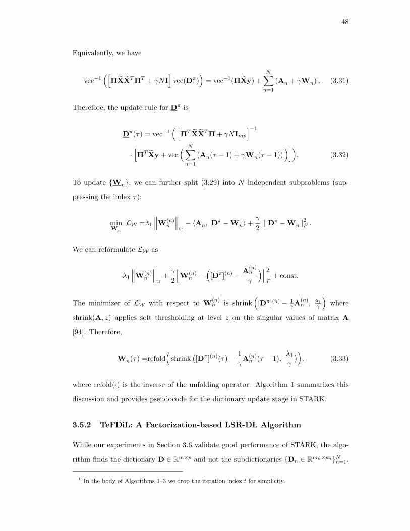
48

Equivalently, we have

vec−1([

ΠXXTΠT + γNI]

vec(Dπ))

= vec−1(ΠXy) +N∑n=1

(An + γWn) . (3.31)

Therefore, the update rule for Dπ is

Dπ(τ) = vec−1( [

ΠT XXTΠ + γNImp

]−1

·[ΠT Xy + vec

( N∑n=1

(An(τ − 1) + γWn(τ − 1)))])

. (3.32)

To update Wn, we can further split (3.29) into N independent subproblems (sup-

pressing the index τ):

minWn

LW =λ1

∥∥∥W(n)n

∥∥∥tr− 〈An, Dπ −Wn〉+

γ

2‖ Dπ −Wn‖

2F .

We can reformulate LW as

λ1

∥∥∥W(n)n

∥∥∥tr

+γ

2

∥∥∥W(n)n −

([Dπ](n) − A

(n)n

γ

)∥∥∥2

F+ const.

The minimizer of LW with respect to W(n)n is shrink

([Dπ](n) − 1

γA(n)n , λ1

γ

)where

shrink(A, z) applies soft thresholding at level z on the singular values of matrix A

[94]. Therefore,

Wn(τ) =refold(

shrink([Dπ](n)(τ)− 1

γA(n)n (τ − 1),

λ1

γ

)), (3.33)

where refold(·) is the inverse of the unfolding operator. Algorithm 1 summarizes this

discussion and provides pseudocode for the dictionary update stage in STARK.

3.5.2 TeFDiL: A Factorization-based LSR-DL Algorithm

While our experiments in Section 3.6 validate good performance of STARK, the algo-

rithm finds the dictionary D ∈ Rm×p and not the subdictionaries Dn ∈ Rmn×pnNn=1.

11In the body of Algorithms 1–3 we drop the iteration index t for simplicity.

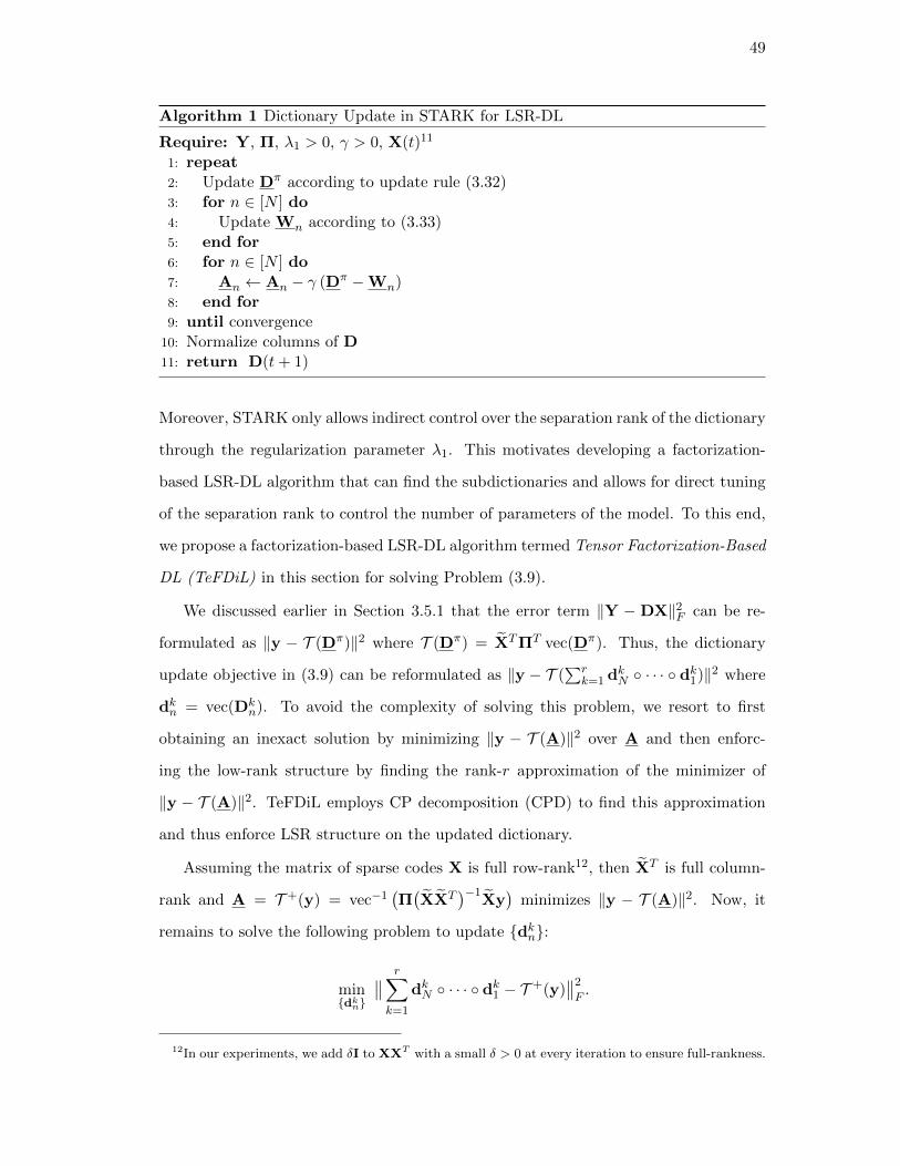
49

Algorithm 1 Dictionary Update in STARK for LSR-DL

Require: Y, Π, λ1 > 0, γ > 0, X(t)11

1: repeat2: Update Dπ according to update rule (3.32)3: for n ∈ [N ] do4: Update Wn according to (3.33)5: end for6: for n ∈ [N ] do7: An ← An − γ (Dπ −Wn)8: end for9: until convergence

10: Normalize columns of D11: return D(t+ 1)

Moreover, STARK only allows indirect control over the separation rank of the dictionary

through the regularization parameter λ1. This motivates developing a factorization-

based LSR-DL algorithm that can find the subdictionaries and allows for direct tuning

of the separation rank to control the number of parameters of the model. To this end,

we propose a factorization-based LSR-DL algorithm termed Tensor Factorization-Based

DL (TeFDiL) in this section for solving Problem (3.9).

We discussed earlier in Section 3.5.1 that the error term ‖Y − DX‖2F can be re-

formulated as ‖y − T (Dπ)‖2 where T (Dπ) = XTΠT vec(Dπ). Thus, the dictionary

update objective in (3.9) can be reformulated as ‖y − T (∑r

k=1 dkN · · · dk1)‖2 where

dkn = vec(Dkn). To avoid the complexity of solving this problem, we resort to first

obtaining an inexact solution by minimizing ‖y − T (A)‖2 over A and then enforc-

ing the low-rank structure by finding the rank-r approximation of the minimizer of

‖y − T (A)‖2. TeFDiL employs CP decomposition (CPD) to find this approximation

and thus enforce LSR structure on the updated dictionary.

Assuming the matrix of sparse codes X is full row-rank12, then XT is full column-

rank and A = T +(y) = vec−1(Π(XXT

)−1Xy)

minimizes ‖y − T (A)‖2. Now, it

remains to solve the following problem to update dkn:

mindkn

∥∥ r∑k=1

dkN · · · dk1 − T +(y)∥∥2

F.

12In our experiments, we add δI to XXT with a small δ > 0 at every iteration to ensure full-rankness.

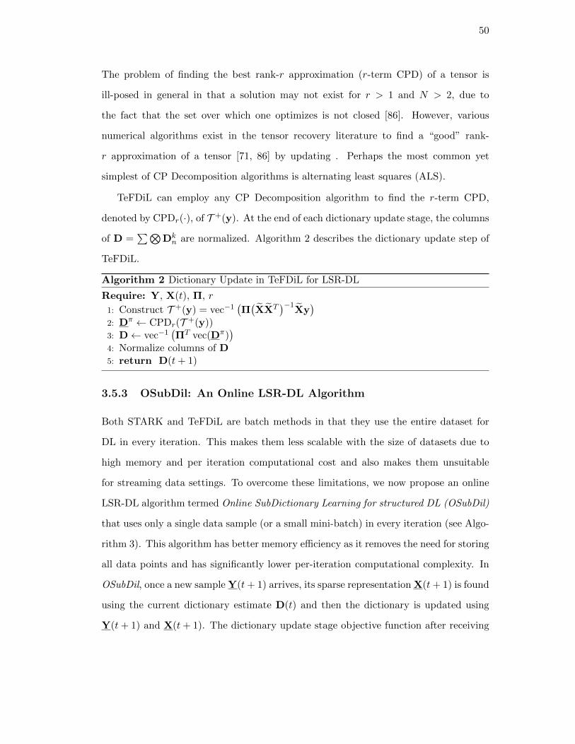
50

The problem of finding the best rank-r approximation (r-term CPD) of a tensor is

ill-posed in general in that a solution may not exist for r > 1 and N > 2, due to

the fact that the set over which one optimizes is not closed [86]. However, various

numerical algorithms exist in the tensor recovery literature to find a “good” rank-

r approximation of a tensor [71, 86] by updating . Perhaps the most common yet

simplest of CP Decomposition algorithms is alternating least squares (ALS).

TeFDiL can employ any CP Decomposition algorithm to find the r-term CPD,

denoted by CPDr(·), of T +(y). At the end of each dictionary update stage, the columns

of D =∑⊗

Dkn are normalized. Algorithm 2 describes the dictionary update step of

TeFDiL.

Algorithm 2 Dictionary Update in TeFDiL for LSR-DL

Require: Y, X(t), Π, r

1: Construct T +(y) = vec−1(Π(XXT

)−1Xy)

2: Dπ ← CPDr(T +(y))3: D← vec−1

(ΠT vec(Dπ)

)4: Normalize columns of D5: return D(t+ 1)

3.5.3 OSubDil: An Online LSR-DL Algorithm

Both STARK and TeFDiL are batch methods in that they use the entire dataset for

DL in every iteration. This makes them less scalable with the size of datasets due to

high memory and per iteration computational cost and also makes them unsuitable

for streaming data settings. To overcome these limitations, we now propose an online

LSR-DL algorithm termed Online SubDictionary Learning for structured DL (OSubDil)

that uses only a single data sample (or a small mini-batch) in every iteration (see Algo-

rithm 3). This algorithm has better memory efficiency as it removes the need for storing

all data points and has significantly lower per-iteration computational complexity. In

OSubDil, once a new sample Y(t+ 1) arrives, its sparse representation X(t+ 1) is found

using the current dictionary estimate D(t) and then the dictionary is updated using

Y(t+ 1) and X(t+ 1). The dictionary update stage objective function after receiving

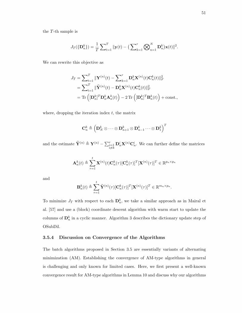
51

the T -th sample is

JT (Dkn) =

1

T

∑T

t=1‖y(t)−

(∑r

k=1

⊗N

n=1Dkn

)x(t)‖2.

We can rewrite this objective as

JT =∑T

t=1‖Y(n)(t)−

∑r

k=1DknX

(n)(t)Ckn(t)‖2F

=∑T

t=1‖Y(n)(t)−Dk

nX(n)(t)Ck

n(t)‖2F

= Tr(

[Dkn]TDk

nAkn(t)

)− 2 Tr

([Dk

n]TBkn(t)

)+ const.,

where, dropping the iteration index t, the matrix

Ckn ,

(DkN ⊗ · · · ⊗Dk

n+1 ⊗Dkn−1 · · · ⊗Dk

1

)Tand the estimate Y(n) , Y(n) −

∑ri=1i 6=k

DinX

(n)Cin. We can further define the matrices

Akn(t) ,

t∑τ=1

X(n)(t)Ckn(τ)[Ck

n(τ)]T [X(n)(τ)]T ∈ Rpn×pn

and

Bkn(t) ,

t∑τ=1

Y(n)(τ)[Ckn(τ)]T [X(n)(τ)]T ∈ Rmn×pn .

To minimize JT with respect to each Dkn, we take a similar approach as in Mairal et

al. [57] and use a (block) coordinate descent algorithm with warm start to update the

columns of Dkn in a cyclic manner. Algorithm 3 describes the dictionary update step of

OSubDil.

3.5.4 Discussion on Convergence of the Algorithms

The batch algorithms proposed in Section 3.5 are essentially variants of alternating

minimization (AM). Establishing the convergence of AM-type algorithms in general

is challenging and only known for limited cases. Here, we first present a well-known

convergence result for AM-type algorithms in Lemma 10 and discuss why our algorithms

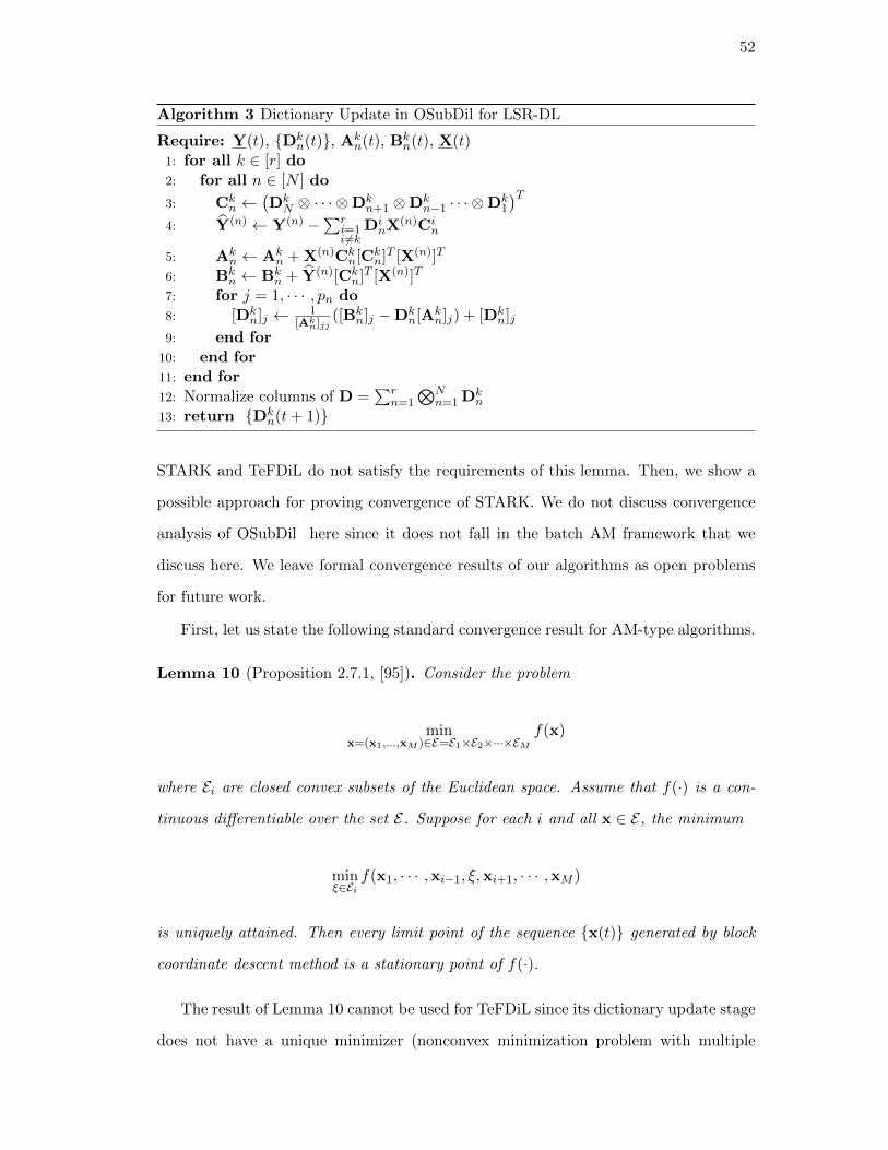
52

Algorithm 3 Dictionary Update in OSubDil for LSR-DL

Require: Y(t), Dkn(t), Ak

n(t), Bkn(t), X(t)

1: for all k ∈ [r] do2: for all n ∈ [N ] do

3: Ckn ←

(DkN ⊗ · · · ⊗Dk

n+1 ⊗Dkn−1 · · · ⊗Dk

1

)T4: Y(n) ← Y(n) −

∑ri=1i 6=k

DinX

(n)Cin

5: Akn ← Ak

n + X(n)Ckn[Ck

n]T [X(n)]T

6: Bkn ← Bk

n + Y(n)[Ckn]T [X(n)]T

7: for j = 1, · · · , pn do8: [Dk

n]j ← 1[Akn]jj

([Bkn]j −Dk

n[Akn]j) + [Dk

n]j

9: end for10: end for11: end for12: Normalize columns of D =

∑rn=1

⊗Nn=1 Dk

n

13: return Dkn(t+ 1)

STARK and TeFDiL do not satisfy the requirements of this lemma. Then, we show a

possible approach for proving convergence of STARK. We do not discuss convergence

analysis of OSubDil here since it does not fall in the batch AM framework that we

discuss here. We leave formal convergence results of our algorithms as open problems

for future work.

First, let us state the following standard convergence result for AM-type algorithms.

Lemma 10 (Proposition 2.7.1, [95]). Consider the problem

minx=(x1,...,xM )∈E=E1×E2×···×EM

f(x)

where Ei are closed convex subsets of the Euclidean space. Assume that f(·) is a con-

tinuous differentiable over the set E. Suppose for each i and all x ∈ E, the minimum

minξ∈Ei

f(x1, · · · ,xi−1, ξ,xi+1, · · · ,xM )

is uniquely attained. Then every limit point of the sequence x(t) generated by block

coordinate descent method is a stationary point of f(·).

The result of Lemma 10 cannot be used for TeFDiL since its dictionary update stage

does not have a unique minimizer (nonconvex minimization problem with multiple

53

global minima)). Moreover, as discussed in Section 3.5.2, TeFDiL only returns an

inexact solution.

Similarly, this result cannot be used to show convergence of STARK to a stationary

point of Problem (3.8) due to the fact that the constraint set Dm×p is not convex.

However, we show next that dropping the unit column-norm constraint allows us to

provide certain convergence guarantees. The unit column-norm constraint is essential in

standard DL algorithms since in its absence, the `1 norm regularization term encourages

undesirable solutions where ‖X‖F is very small while ‖D‖F is very large. However, in

the regularization-based LSR-DL problem, the additional regularization term ‖Dπ‖strensures this does not happen. Therefore, dropping the unit column-norm constraint is

sensible in this problem.

Let us discuss what guarantees we are able to obtain after relaxing the constraint

set Dm×p. Consider the minimization problem

minD∈Rm×p,X∈Rp×L

‖Y −DX‖2F + λ1 ‖Dπ‖str + λ‖X‖1,1. (3.34)

We show that under the following assumptions, STARK converges to a stationary point

of Problem (3.34) (when the normalization step is not enforced). Then we discuss how

this problem is related to Problem (3.8).

Assumption 4. Consider the sequence(D(t),X(t)

)generated by STARK. We assume

that for all t ≥ 0:

I) Classical optimality conditions for the lasso problem (see Tibshirani [96]) are sat-

isfied.

II) X(t) is full row-rank at all t.

Proposition 1 establishes the convergence of STARK (without normalization).

Proposition 1. Under Assumption 4, STARK converges to a stationary point of prob-

lem (3.34).

Proof. We invoke Lemma 10 to show the convergence of STARK. To use this lemma,

54

the minimization problem w.r.t. each block needs to correspond to a closed convex

constraint set and also needs to have a unique minimizer.

In the sparse coding stage, given Assumption 4-I, the minimizer of the lasso problem

is unique. In the dictionary update stage of STARK, the objective of problem (3.34)

is strongly convex w.r.t. D under Assumption 4-II and thus has a unique minimizer.

Moreover, the constraint set Rp×L is closed and convex. To utilize Lemma 10, it remains

to show that this minimum is actually attained by ADMM. To this end, we restate

Problem (3.26) as

minDπ ,W

f1(Dπ) + f2(W)

s.t. W = HDπ, (3.35)

where f1(Dπ) = 12 ‖Y −DX‖2F (note that DX is a linear function of Dπ) and f2(W) =

λ1∑N

n=1

∥∥(Wn)(n)

∥∥∗. It is clear that HH∗ is convertible. Therefore, according to

Lemma 11 stated below, the ADMM algorithm converges to the unique minimizer of

Problem (3.26).

Lemma 11 (Chapter 3, Proposition 4.2, [97]). Consider the problem

minx∈C1,z∈C2

f1(x) + f2(z)

s.t. z = A(x) (3.36)

Then, if AA∗ is invertible or if C1 is bounded, the sequence generated by the ADMM

algorithm applied to the Augmented Lagrangian function converges to an optimum of

(3.36).

This concludes the proof.

So far we discussed convergence of STARK to Problem (3.34) while our identi-

fiability results are for problem (3.8). There is, however, a strong connection be-

tween minimization Problems (3.8) and (3.34): for each local minimum D of prob-

lem (3.8), there exists an X such that (D, X) is a local minimum of (3.34). Define

55

`regY (D,X) = 1

L ‖Y −DX‖2F+λ1 ‖Dπ‖str+λL‖X‖1,1. Consider any D that is a local min-

imum of (3.8) and let X = argminX∈Rp×L `regY (D,X). We have `reg

Y (D, X) = F regY (D).

Since D is a local minimizer of F regY (D), F reg

Y (D) ≤ F regY (D) for any D in the lo-

cal neighborhood of D. Also by definition, F regY (D) ≤ `reg

Y (D,X) for any X. Thus,

`regY (D, X) ≤ `reg

Y (D,X) for any (D,X) in the local neighborhood of (D, X), meaning

that (D, X) is a local minimizer of (3.34). Since we showed in Section 3.4 that a local

minimum D∗ of (3.8) is close to the true dictionary D0, we can say there is a local

minimum (D∗,X∗) of (3.34) such that D∗ is close to D0. So our recovery result for

(3.8) can apply to our proposed algorithm for solving (3.34) as well.

3.6 Numerical Experiments

We evaluate our algorithms on synthetic and real-world datasets to understand the

impact of training set size and noise level on the performance of LSR-DL. In particular,

we want to understand the effect of exploiting additional structure in representation

accuracy and denoising performance. We compare the performance of our proposed

algorithms with existing DL algorithms in each scenario and show that in almost every

case our proposed LSR-DL algorithms outperform K-SVD. Our results also offer in-

sights into how the size and quality of training data can affect the choice of the proper

DL model. Specifically, our experiments on image denoising show that when noise level

in data is high, TeFDiL performs best when the separation rank is 1. On the other

hand, in low noise regimes, the performance of TeFDiL improves as we increase the

separation rank. Furthermore, our synthetic experiments confirm that when the true

underlying dictionary follows the KS (LSR) structure, our structured algorithms clearly

outperform K-SVD, especially when the number of training samples is very small. This

implies the potential of the LSR-DL model and our algorithms in applications where

the true dictionary follows the LSR structure more closely.

Synthetic Experiments: We compare our algorithms to K-SVD[13] (standard

DL) as well as a simple block coordinate descent (BCD) algorithm that alternates

between updating every subdictionary in problem (3.9). This BCD algorithm can be

interpreted as an extension of the KS-DL algorithm [79] for the LSR model. We show

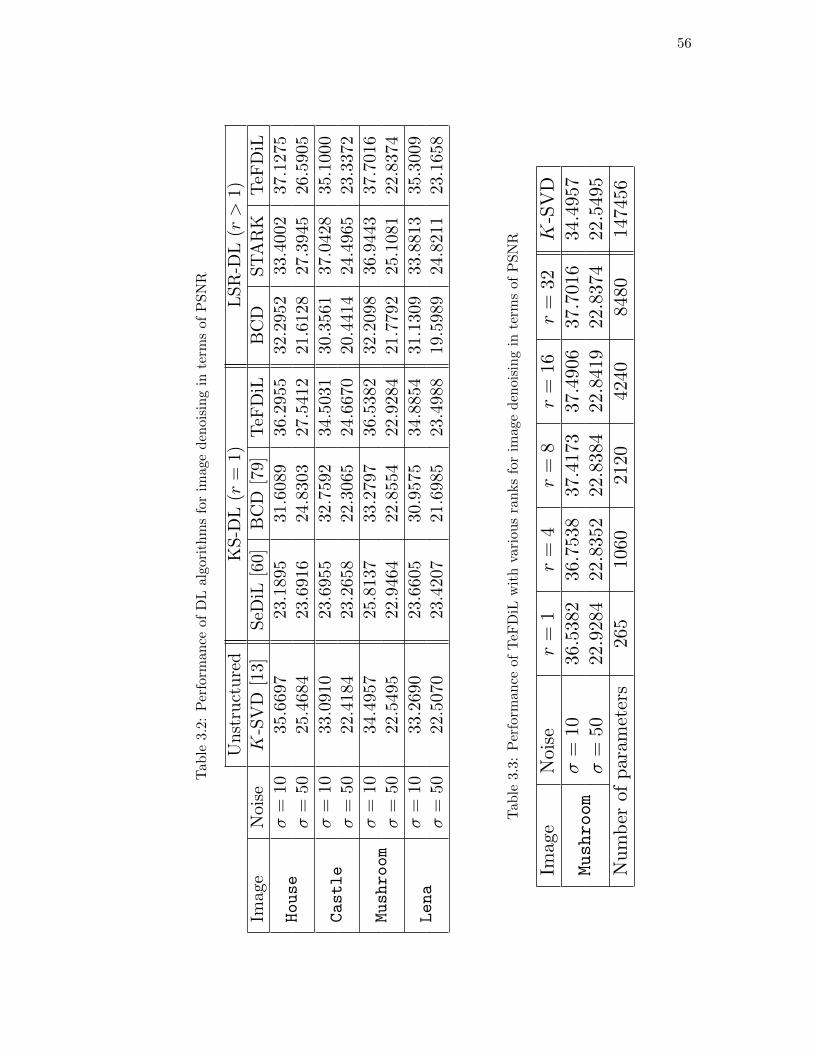
56

Tab

le3.2

:P

erfo

rman

ceof

DL

algo

rith

ms

for

imag

eden

oisi

ng

inte

rms

ofP

SN

R

Unst

ruct

ure

dK

S-D

L(r

=1)

LSR

-DL

(r>

1)

Image

Noi

seK

-SV

D[1

3]

SeD

iL[6

0]B

CD

[79]

TeF

DiL

BC

DST

AR

KT

eFD

iL

House

σ=

10

35.6

697

23.1

895

31.6

089

36.2

955

32.2

952

33.4

002

37.1

275

σ=

50

25.4

684

23.6

916

24.8

303

27.5

412

21.6

128

27.3

945

26.5

905

Castle

σ=

10

33.0

910

23.6

955

32.7

592

34.5

031

30.3

561

37.0

428

35.1

000

σ=

50

22.4

184

23.2

658

22.3

065

24.6

670

20.4

414

24.4

965

23.3

372

Mushroom

σ=

10

34.4

957

25.8

137

33.2

797

36.5

382

32.2

098

36.9

443

37.7

016

σ=

50

22.5

495

22.9

464

22.8

554

22.9

284

21.7

792

25.1

081

22.8

374

Lena

σ=

10

33.2

690

23.6

605

30.9

575

34.8

854

31.1

309

33.8

813

35.3

009

σ=

50

22.5

070

23.4

207

21.6

985

23.4

988

19.5

989

24.8

211

23.1

658

Tab

le3.3

:P

erfo

rman

ceof

TeF

DiL

wit

hva

riou

sra

nks

for

imag

ed

enoi

sin

gin

term

sof

PS

NR

Imag

eN

ois

er

=1

r=

4r

=8

r=

16r

=32

K-S

VD

Mushroom

σ=

10

36.5

382

36.7

538

37.4

173

37.4

906

37.7

016

34.4

957

σ=

50

22.9

284

22.8

352

22.8

384

22.8

419

22.8

374

22.5

495

Nu

mb

erof

par

am

eter

s26

510

6021

2042

4084

80

1474

56

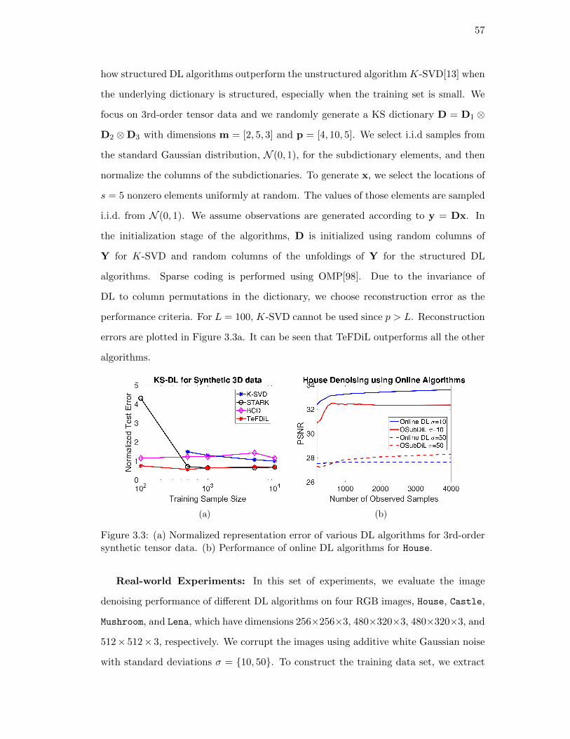
57

how structured DL algorithms outperform the unstructured algorithm K-SVD[13] when

the underlying dictionary is structured, especially when the training set is small. We

focus on 3rd-order tensor data and we randomly generate a KS dictionary D = D1 ⊗

D2 ⊗D3 with dimensions m = [2, 5, 3] and p = [4, 10, 5]. We select i.i.d samples from

the standard Gaussian distribution, N (0, 1), for the subdictionary elements, and then

normalize the columns of the subdictionaries. To generate x, we select the locations of

s = 5 nonzero elements uniformly at random. The values of those elements are sampled

i.i.d. from N (0, 1). We assume observations are generated according to y = Dx. In

the initialization stage of the algorithms, D is initialized using random columns of

Y for K-SVD and random columns of the unfoldings of Y for the structured DL

algorithms. Sparse coding is performed using OMP[98]. Due to the invariance of

DL to column permutations in the dictionary, we choose reconstruction error as the

performance criteria. For L = 100, K-SVD cannot be used since p > L. Reconstruction

errors are plotted in Figure 3.3a. It can be seen that TeFDiL outperforms all the other

algorithms.

(a) (b)

Figure 3.3: (a) Normalized representation error of various DL algorithms for 3rd-ordersynthetic tensor data. (b) Performance of online DL algorithms for House.

Real-world Experiments: In this set of experiments, we evaluate the image

denoising performance of different DL algorithms on four RGB images, House, Castle,

Mushroom, and Lena, which have dimensions 256×256×3, 480×320×3, 480×320×3, and

512× 512× 3, respectively. We corrupt the images using additive white Gaussian noise

with standard deviations σ = 10, 50. To construct the training data set, we extract

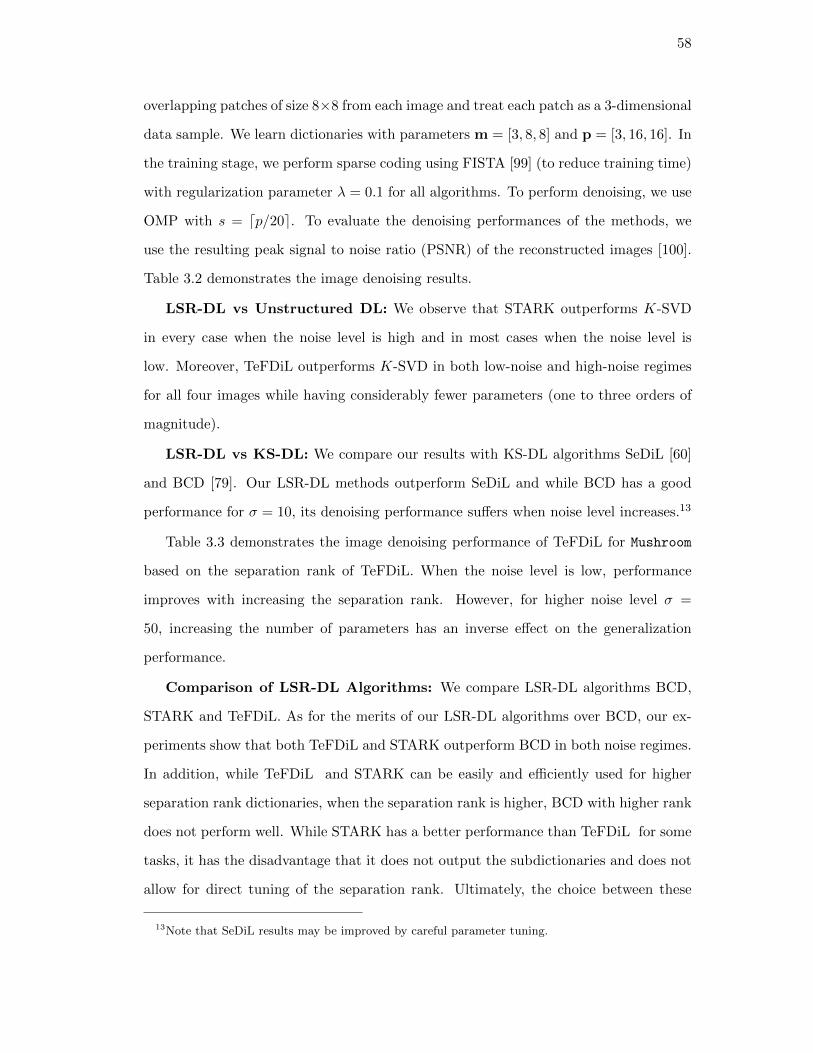
58

overlapping patches of size 8×8 from each image and treat each patch as a 3-dimensional

data sample. We learn dictionaries with parameters m = [3, 8, 8] and p = [3, 16, 16]. In

the training stage, we perform sparse coding using FISTA [99] (to reduce training time)

with regularization parameter λ = 0.1 for all algorithms. To perform denoising, we use

OMP with s = dp/20e. To evaluate the denoising performances of the methods, we

use the resulting peak signal to noise ratio (PSNR) of the reconstructed images [100].

Table 3.2 demonstrates the image denoising results.

LSR-DL vs Unstructured DL: We observe that STARK outperforms K-SVD

in every case when the noise level is high and in most cases when the noise level is

low. Moreover, TeFDiL outperforms K-SVD in both low-noise and high-noise regimes

for all four images while having considerably fewer parameters (one to three orders of

magnitude).

LSR-DL vs KS-DL: We compare our results with KS-DL algorithms SeDiL [60]

and BCD [79]. Our LSR-DL methods outperform SeDiL and while BCD has a good

performance for σ = 10, its denoising performance suffers when noise level increases.13

Table 3.3 demonstrates the image denoising performance of TeFDiL for Mushroom

based on the separation rank of TeFDiL. When the noise level is low, performance

improves with increasing the separation rank. However, for higher noise level σ =

50, increasing the number of parameters has an inverse effect on the generalization

performance.

Comparison of LSR-DL Algorithms: We compare LSR-DL algorithms BCD,

STARK and TeFDiL. As for the merits of our LSR-DL algorithms over BCD, our ex-

periments show that both TeFDiL and STARK outperform BCD in both noise regimes.

In addition, while TeFDiL and STARK can be easily and efficiently used for higher

separation rank dictionaries, when the separation rank is higher, BCD with higher rank

does not perform well. While STARK has a better performance than TeFDiL for some

tasks, it has the disadvantage that it does not output the subdictionaries and does not

allow for direct tuning of the separation rank. Ultimately, the choice between these

13Note that SeDiL results may be improved by careful parameter tuning.

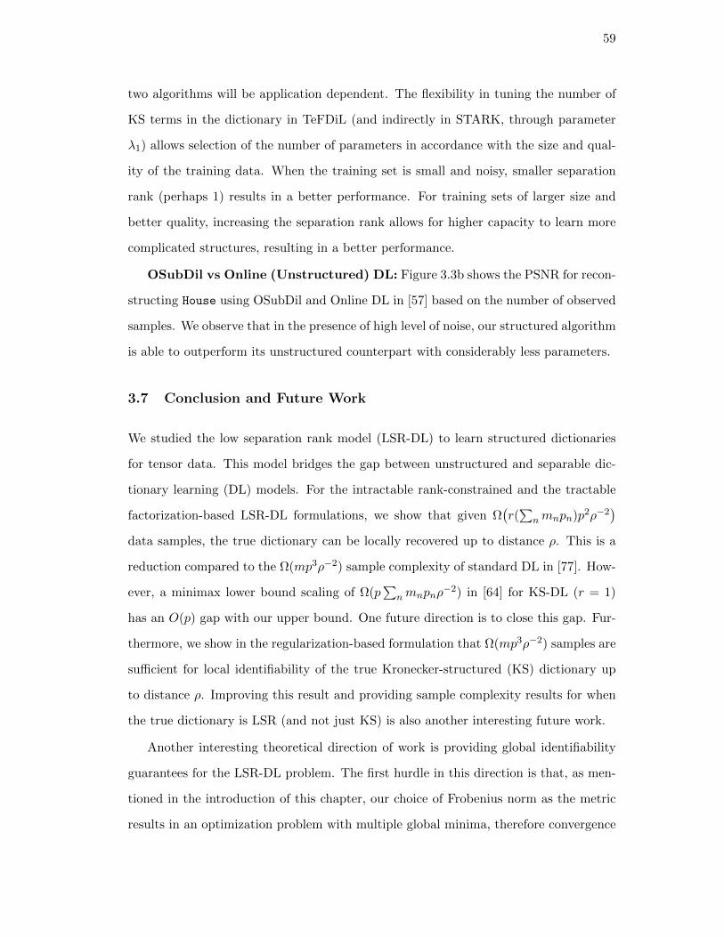
59

two algorithms will be application dependent. The flexibility in tuning the number of

KS terms in the dictionary in TeFDiL (and indirectly in STARK, through parameter

λ1) allows selection of the number of parameters in accordance with the size and qual-

ity of the training data. When the training set is small and noisy, smaller separation

rank (perhaps 1) results in a better performance. For training sets of larger size and

better quality, increasing the separation rank allows for higher capacity to learn more

complicated structures, resulting in a better performance.

OSubDil vs Online (Unstructured) DL: Figure 3.3b shows the PSNR for recon-

structing House using OSubDil and Online DL in [57] based on the number of observed

samples. We observe that in the presence of high level of noise, our structured algorithm

is able to outperform its unstructured counterpart with considerably less parameters.


We studied the low separation rank model (LSR-DL) to learn structured dictionaries

for tensor data. This model bridges the gap between unstructured and separable dic-

tionary learning (DL) models. For the intractable rank-constrained and the tractable

factorization-based LSR-DL formulations, we show that given Ω(r(∑

nmnpn)p2ρ−2)

data samples, the true dictionary can be locally recovered up to distance ρ. This is a

reduction compared to the Ω(mp3ρ−2) sample complexity of standard DL in [77]. How-

ever, a minimax lower bound scaling of Ω(p∑

nmnpnρ−2) in [64] for KS-DL (r = 1)

has an O(p) gap with our upper bound. One future direction is to close this gap. Fur-

thermore, we show in the regularization-based formulation that Ω(mp3ρ−2) samples are

sufficient for local identifiability of the true Kronecker-structured (KS) dictionary up

to distance ρ. Improving this result and providing sample complexity results for when

the true dictionary is LSR (and not just KS) is also another interesting future work.

Another interesting theoretical direction of work is providing global identifiability

guarantees for the LSR-DL problem. The first hurdle in this direction is that, as men-

tioned in the introduction of this chapter, our choice of Frobenius norm as the metric

results in an optimization problem with multiple global minima, therefore convergence

60

to a global minimum does not necessarily mean global identifiability. An interesting fu-

ture direction is to consider alternative (permutation and sign-invariant) distances that

result in a single global minimum. The second obstacle in this direction is the difficulty

in establishing global convergence results for nonconvex optimization problems. In the

recent years, researchers have proposed DL algorithms guaranteed to converge to global

optimizers of the nonconvex DL problem [80, 101, 102]. Moreover, Sun et al. [103] show

that for the special case of complete dictionary learning, the local minima of the prob-

lem are all globally optimum and the saddle points are escapable. While establishing

local identifiability is an important first step, obtaining geometric characterization of

the optimization landscape of the LSR-DL problem and developing algorithms with

global convergence guarantees is an interesting future direction.

Finally, we presented two LSR-DL algorithms and showed that they have better

generalization performance for image denoising in comparison to unstructured DL al-

gorithm K-SVD [13] and existing KS-DL algorithms SeDiL [60] and BCD [79]. We

also present OSubDil that to the best our knowledge is the first online algorithm that

results in LSR or KS dictionaries. We show that OSubDil results in a faster reduction

in the reconstruction error in terms of number of observed samples compared to the

state-of-the-art online DL algorithm [57] when the noise level in data is high.

The experimental and theoretical results in this chapter and in the related literature

showcase the benefits of exploiting tensor structure of data in the dictionary learning

problem. Inspired by these results, in the next chapter we study the benefits of exploit-

ing tensor structure of data in another learning problem, namely the linear regression.

Some of the analytical tools used in this chapter will also prove useful in our analysis

of tensor linear regression in the next chapter.

61

Chapter 4

Tensor Regression

In this chapter, we study a tensor-structured linear regression model with tensor-

structured predictor and regression parameters and scalar response variables. We focus

on the fundamental limits on the accuracy and the sample complexity of estimating

the tensor-valued regression parameters (regression tensors) in this model. Specifically,

we obtain a lower bound on the minimax risk of estimating the underlying N -th order

regression tensor B∗ ∈ Rm1×···×mN from L predictor-response pairs (Xl, yl). By com-

paring this lower bound to the known lower bounds for standard linear regression, we

provide an insight into the benefits of exploiting the tensor structure of B∗ in tensor

linear regression.

4.1 Introduction

Many modern machine learning and data science problems involve high dimensional

multiway (tensor) structures. Examples of problems wherein tensors have found appli-

cations include (but are not limited to) recommendation systems [74, 104–106], mixture

and topic modeling [107, 108], deep learning [73, 109–113], multilinear subspace learn-

ing [114, 115], and speech source separation [116, 117]. As we discussed in Chapter 3,

taking advantage of the structured and the higher order correlations in tensor structures

reduces the dimensionality of the problem and can result in more accurate predictions

or estimations (or equivalently lowering sample complexity required to obtain a target

accuracy). In this chapter, we study low-rank tensor linear regression (TLR), a class

of supervised learning models that aim to exploit the tensor structure in the predictors

and the regression parameters to allow for solving high dimensional linear regression

problems accurately when the number of observations is only a small fraction of the

62

number predictors. Tensor linear regression has application in many areas including

multitask learning [88], complex network analysis [118], and neuroimaging data analysis

[119, 120].

Tensor regression models methods share the assumption that the model parameters

form a high order tensor and there exists a low dimensional factorization for the re-

gression tensor. The model we consider here is based on CANDECOMP/PARAFAC

(CP) decompostion of tensors which allows for explicit accounting of interdependencies

along different modes of tensor arrays.

Here, we focus on providing lower bounds on minimax risk of estimating the regres-

sion tensor using any estimator. By comparing these bounds to those of standard (i.e.

vectorized) linear regression, we show the benefits of exploiting the tensor structure in

the linear regression problem with tensor-structured predictors and parameters. For

standard linear regression, the lower bound on the minimax risk of estimating a pa-

rameter vector in Rm is Ω(

mσ2

L‖Σx‖2

)where Σx is the covariance matrix of the predictor

vector and σ is the noise variance [121]. Therefore, by vectorizing tensor data samples

in Rm1×m2×···×mN , we have a lower bound on the worst case MSE of estimating the

true model parameters in form of

ε∗ ≥ Ω(∏N

n=1mnσ2

L‖Σx‖2

). (4.1)

In contrast, we show that when the spatial structure of data is preserved and a CP-rank-

p structure is imposed on the parameter tensor, the minimax lower bound is reduced

to

ε∗ ≥ Ω(σ2p

∑Nn=1mn

NL‖Σx‖2

). (4.2)


Tensor decompositions have received a lot of attention in the recent years as a tool to

avoid overparameterization in tensor data models [71, 72, 122]. The resulting more com-

pact models tend to be more efficient with regards to storage, computational complexity,

63

and generalization performance. This has motivated the use of tensor decompositions

in a variety of areas, including deep learning [73, 109], collaborative filtering [74, 105],

multilinear subspace learning [114], source separation [116], topic modeling [108], and

many other works [74]. In the recent years, tensor decompositions have also received

attention in regression problems such as neuroimaging data analysis [119, 120] where

data is tensor structured and high dimensional but the sample size is relatively small.

While some works in the literature consider tensor linear regression problems with

tensor responses [123–126], our focus in this work is on the model with scalar response.

A majority of the works on tensor linear regression (TLR) focus on the algorithmic

aspects of TLR and developing efficient solvers for the problem under different settings

[119, 120, 127–134]. In contrast, fewer works study the theoretical aspect of the TLR

problem in terms of the fundamental limits of the TLR models. Wimalawarne et al.

study regularized tensor regression with different choices of the regularization term

and derive excess risk bounds for each regularized model. Zhou et al. [119] study the

conditions for local identifiablity of the true parameter tensor in CP-based TLR model.

The CP-based model assumes that the parameter tensor has a low-CP-rank structure

(i.e. the CP-rank is at most p for some small p). The authors show that the required

number of samples for idetifiability is reduced from Ω(∏N

n=1mn

)to Ω

(p∑N

n=1mn

). In

the same vein, Li et al. [120] investigate the TLR model based on Tucker decomposition,

where the assumption is that the Tucker-rank of the parameter tensor is small. The

authors show that, similar to the CP-based model, the required sample complexity for

local identifiability of the true tensor is a linear function of the number of parameters

(degrees of freedom) in the model. In terms of works on the minimax risk in TLR,

Suzuki [135] obtain results for CP-based tensor completion (which can be though of

as a special case of tensor regression, where the elements of predictor tensors are all

zero except for a single element with value 1). Their result, however, does not trivially

extend to the general TLR problem. To the best of our knowledge, our work is the first

result on minimax risk in the general CP-based TLR model.

Our approach for deriving minimax result is a well-established information theoretic

method that was first proposed by Khas’minskii [136] and was later developed further

64

by other researchers [137, 138]. Specifically, because of our analysis of tensor-structured

parameters, our proofs borrow many analytical tools from the works by Jung et al. [139]

and Shakeri et al. [64, 140].


4.2.1 Notation and Definitions

We use underlined bold upper-case (A), bold upper-case (A), bold lower-case (a),

and lower-case (a) letters to denote tensors, matrices, vectors, and scalars, respec-

tively. For any integer p, we define [p] , 1, 2, · · · , p. We denote by AnNn=1 the set

A1, · · · ,AN. We drop the range indicators if they are clear from the context.

Norms and inner products: We denote by ‖v‖p the `p norm of vector v, while

we use ‖A‖2 and ‖A‖F to denote the spectral and the Frobenius norm of matrix

A, respectively. We define by ‖A‖0 the number of nonzero elements of matrix (or

vector) A. We define the inner product of two tensors (or matrices) A and B as

〈A,B〉 , 〈vec(A), vec(B)〉 where vec(·) is the vectorization operator.

Matrix products: We denote the Hadamard product (element-wise product) of ma-

trices A ∈ Rm×p and B ∈ Rm×p by A •B ∈ Rm×p. We denote by A⊗B ∈ Rm1m2×p1p2

the Kronecker product of matrices A ∈ Rm1×p1 and B ∈ Rm2×p2 . We use⊗N

n=1 Ai ,

A1⊗A2⊗· · ·⊗AN for the Kronecker product of N matrices. The Khatri-Rao product

of two matrices C ∈ Rm1×p and D ∈ Rm2×p is denoted by CD ∈ Rm1m2×p. We use⊙Nn=1 Ci , C1 C2 · · · CN for the Khatri-Rao product of N matrices.

Definitions for tensors: We denote the outer product (tensor product) of vectors

by , while ×n denotes the mode-n product between a tensor and a matrix. An N -

way tensor is rank-1 if it can be written as outer product of N vectors: v1 · · · vN .

A superdiagonal tensor S ∈ Rm1×m2×···×mN is a tensor with all zero elements except

for the superdiagonal elements, i.e., the elements indexed by (i1, i2, · · · , iN ) such that

i1 = i2 = · · · = iN . We denote by SNp the set of all N -way superdiagonal tensors in

Rp×p×···×p.

Throughout this chapter, by the rank of a tensor, rank(A), we mean the CP-rank

65

of A, the minimum number of rank-1 tensors that construct A as their sum. The CP

decomposition (CPD), decomposes a tensor into sum of its rank-1 tensor components.

The Tucker decomposition factorizes an N -way tensor A ∈ Rm1×m2×···×mN as A =

X ×1 D1 ×2 D2 ×3 · · · ×N DN , where X ∈ Rp1×p2×···×pN denotes the core tensor and

Dn ∈ Rmn×pn denote factor matrices along the n-th mode of A for n ∈ [N ].

Notations for functions and spaces: We denote by Dm×p the oblique manifold in

Rm×p; the manifold of matrices with unit-norm columns: Dm×p , D ∈ Rm×p|∀j ∈

[p], dTj dj = 1.

4.2.2 Low-Rank Tensor Linear Regression

In tensor linear regression we assume that each scalar response yl ∈ R is generated

according to

yl = 〈B∗,Xl〉+ εl, (4.3)

where B∗ ∈ Rm1×···×mN is the true underlying regression tensor, Xl ∈ Rm1×···×mN Ll=1

is the corresponding (randomly generated) predictor tensor, and εl ∈ R is the obser-

vation noise. In order to explicitly account for the tensor structure in the coefficient

tensor, we adopt a tensor-factorization based model. While there are many ways to

factorize a tensor, we consider a model based on well-known tensor factorization called

the CANDECOMP/PARAFAC (CP) decomposition (Also known as the tensor rank

decomposition1). The CP decomposition factorizes a tensor into sum of its rank-1

tensor components:

A =

r∑k=1

λkak1 · · · akN , (4.4)

1Sometimes CP decomposition is is considered as the generalization of the tensor rank decompositionwhere the number of the terms can be larger than the rank of the tensor. In this Chapter, however,we use only consider the case with minimal number of terms (minimal CP decomposition) and use thetwo names interchangeably.

66

where akn is a unit-norm vector for k ∈ [r] and n ∈ [N ]. When the number of terms r is

minimal in the above expression, then r is called the CP-rank of the tensor2. Therefore

we can write the underlying low-rank coefficient tensor B∗ as

B∗ =

p∑j=1

g∗j b∗1,j · · · b∗N,j ,

where p is small (p mini

∏n 6=i

mn). We can write the CP decomposition of B∗ in the

following more compressed way

B∗ = G∗ ×1 β∗1 · · · ×N β∗N ∈ B, (4.5)

where the set B is defined as

B = G×1 β1 ×2 · · · ×N βN |G ∈ SNp , βn ∈ Dmn×p, ∀n ∈ [N ], (4.6)

where SNp is the set of N -way superdiagonal tensors in Rp×···×p and Dmn×p is the oblique

manifold3 in Rmn×p. We can then express the tensor regression model in the following

way:

yl = 〈vec(B∗), vec(Xl)〉+ εl

= 〈(βN ⊗ · · · ⊗ β1)vec(G∗), vec(Xl)〉+ εl

=⟨⊗1

n=Nβ∗n vec(G∗), vec(Xl)

⟩+ εl. (4.7)

Therefore, the problem reduces from estimating B∗ to estimating β∗nNn=1 and the

superdiagonal elements of G∗, considerably reducing the number of parameters to be

estimated in the problem.

2Throughout this Chapter, by the rank of a tensor, rank(A), we mean the CP-rank of A.

3The unit-norm condition on columns of βtnn is to simplify the analysis by avoiding the ambiguitystemming from the invariance of CP decomposition to scaling of factor matrices.

67

4.2.3 Minimax Risk

Many learning problems, including linear regression, boil down to estimation problem

where some model parameters need to be estimated. Minimax risk, defined as the low-

est risk achievable by any estimator in the worst possible case allowed in an estimation

problem, is an important theoretical tool in understanding the fundamental limits of

such learning problems. These fundamental limits are in terms of bounds on the per-

formance of estimation (or optimization) algorithms. Such bounds are important in

understanding whether the existing algorithms to solve a problem are optimal (with

respect to a certain metric) or one can still develop more efficient algorithms in that

metric. Moreover, these bounds can be used to compare different approaches in mod-

eling a learning problem and understanding the benefits of exploiting our knowledge of

certain structures in data or the underlying generative model of the data.

Let us now formally define the minimax risk in an estimation problem. let P denote

a family of distributions on a sample space X , and let θ : P → Θ denote a mapping

P → θ(P ). The goal is to estimate the true model parameter θ(P ) based on i.i.d.

observations X1 ∈ X drawn from an unknown distribution P ∈ P. To measure the

error of an estimator of parameter θ, we employ the (semi-)metric ρ : Θ × Θ → R+.

Given a set of observations X1, · · · , XL, the minimax risk achieved by any estimator of

θ is defined as

infθ∈Θ

supP∈P

EP[ρ(θ(X1, · · · , XL), θ(P )

)], (4.8)

where the supremum (representing worst case scenario) is taken over all possible dis-

tributions in P and the infimum is taken over all estimators.

Fano’s inequality: A common technique for finding lower bounds on minimax risk in

estimation problems, which we adopt in this work, involves connecting the estimation

problem to a multiple hypothesis testing problem. Fano’s inequality provides lower

bounds on the error in a multiple hypothesis testing problem, is an essential component

of this technique.

Lemma 12 (Fano’s Inequality). Let V be a random variable taking values in a finite

68

set V with cardinality |V| ≥ 2. Consider any Markov chain V → X → V . Let e denote

the occurrence of V 6= V . Then, we have

H(e) + P(e) log(|V| − 1) ≥ H(V |V ), (4.9)

where H(A) is the entropy of random variable A and H(A|B) is the conditional entropy

of A given B.

4.3 Minimax Risk of Tensor Linear Regression

We wish to put a lower bound on the minimax risk of estimators for estimating the

rank-p coefficients tensor B∗ in the low-rank tenor regression problem, based on obser-

vations (Xl, yl). As mentioned earlier, here we consider the CP-based model where the

observations are generated according to

yl = 〈⊗n∈[N ]

β∗n vec(G∗), vec(Xl)〉+ εl. (4.10)

We further make the following assumptions on the generating model:

Assumption 5 (Model assumptions). We assume that in the generating model (4.10),

we have

1. B∗ ∈ Rm1×···×mN is the true, unknown N -way coefficient tensor.

2. Xl ∈ Rm1×···×mN is the N -way covariate tensor (tensor predictor) with some

known distribution and covariance Σx,

3. εl ∼ N (0, σ2) is zero-mean Gaussian noise, independent and uncorrelated to the

class parameter B∗ and predictor variable Xl.

Under the CP-based model, the tensor linear regression problem reduces to estimating

β∗nNn=1 and the superdiagonal core tensor G∗. For the ease of analysis, we assume

that we have the a priori knowledge of the superdiagonal elements of G∗, and the N

factor matrices remain to be estimated.

69

The analysis that we provide here is local in that we assume that the true coefficients

tensor B∗ lies in a neighborhood of radius r around a fixed reference tensor

B0 = G0 ×1 β01 · · · ×N β0

N ∈ B, (4.11)

denoted by

Br = B ∈ B|ρ(B,B0) < r. (4.12)

where B is defined in (4.6). In this work, we choose the semi-metric ρ(B,B′) is chosen to

be ‖B−B′‖2F . This local analysis avoids ambiguity issues intrinsic to tensor regression

problem due to non-uniqueness of CP decomposition. It is trivial to show, however,

that lower bounds on the minimax risk in the local setting also apply to the global

setting (r →∞).

We define the minimax risk as the worst-case mean squared error (MSE) that can

be obtained by the best rank-p tensor estimator B:

ε∗ , infB

supB∈Br

EB

[‖B−B‖2F

]. (4.13)

Our goal here is to provide a lower bound on ε∗ using an information-theoretic method-

ology that we describe in detail next.

4.3.1 Our Approach

We will follow the information-theoretic approach known as Fano’s method [121, 136–

138]. First, we reduce the problem of estimating B∗ to a multiple hypothesis testing

problem between a finite family of coefficient tensors: BT = B1, ...,BT ∈ Br. In this

approach, we assume that the true dictionary is chosen uniformly at random from the

set BT . If there is an estimator with small enough worst case MSE, then we can use

this estimator to solve the multiple hypothesis testing problem. We then can use Fano’s

inequality that lower bounds the error in multiple hypothesis testing problem which we

will use to provide a lower bound on the worst case MSE of the best estimator, i.e.

70

the minimax error. Now the question becomes how to set up the multiple hypothesis

testing problem such that we can obtain tight lower bounds on the minimax error in

the estimation problem. We discuss this next.

In the hypothesis testing problem, we assume that nature chooses a t∗ uniformly at

random from the index set [T ]. The task is now detecting the true coefficient tensor

Bt∗ ∈ BT using observations (Xl, yl). The following lemma, which is an adaptation of

Proposition 2.3 in Duchi [121], formalizes the relation between this hypothesis testing

problem and the original tensor regression problem.

Lemma 13. Consider the regression model (4.10) with minimax risk ε∗ defined in

(4.13). Let B denote4 an arbitrary estimator for the true coefficient tensor B∗ defined

in model (4.10). Moreover, consider the set BT = B1, · · · ,BT ⊂ Br. consider

the multiple hypothesis testing problem where the the true coefficient tensor is chosen

uniformly at random from BT and is indexed by t∗. Let t(B) denote a minimum distance

detector such that

t(B) = argmint∈[T ]

‖B−Bt‖2F ,

where Bt ∈ Br for all t ∈ [T ]. Then, we have

ε∗ ≥ mint,t′∈[T ]

‖Bt −Bt′‖2F · inf

BP(t(B) 6= t∗). (4.14)

Lemma 13 indicates that in order to obtain tight lower bounds on the minimax

risk, we need to construct BT such that the distance between any two tensors in BT is

large (maximizing the first term in the lower bound (4.14)) while the hypothesis testing

problem is also hard, i.e., two distinct coefficient tensors produce similar observations

(maximizing the second term in the lower bound (4.14)).

More details of the construction will be provided in the proof of Theorem 8, our

main result.

4Throughout this chapter we suppress the dependence B on the random observations (X,y).

71

4.3.2 Main Result

Here, we first state the main result of this chapter on the minimax risk of CP-based

tensor linear regression in Theorem 8 and then discuss the proof of the theorem in both

big picture and detail.

Theorem 8. Consider a tensor linear regression problem with L i.i.d. observations

generated according to model (4.10) where the core tensor G∗ is known. Fix a refer-

ence tensor B0 satisfying (4.11) and a positive constant r and suppose that the true

parameter tensor B∗ in model (4.10) belongs to Br defined in (4.12). Further, assume

that Assumption 5 holds. Then, the minimax lower bound ε∗ defined in (4.13) can be

bounded as follows

ε∗ ≥ t4

min‖G∗‖2F

κ2,‖G∗‖2F r2

2pNκ2,(

c1 p∑N

n=1(mn − 1) +N(1− 1

2 log2N)− 2)σ2

4NL‖Σx‖2p

, (4.15)

where t ≤ minn∈[N ]2

(mn−1)p and 0 < c1 < 1 and κ > 1.

We first provide an outline of the proof, then provide the formal proof.

Outline of the proof of Theorem 8. We set up a multiway hypothesis testing problem by

constructing a set of T distinct tensors in the parameter space BT = B1, · · · ,BT ∈ Br

where

Br , B ∈ B| ‖B−B0‖F < r, (4.16)

such that

mint,t′∈[T ]

‖Bt −Bt′‖2F ≥ 2δ. (4.17)

for some positive value δ. The true coefficient tensor, indexed by t∗, then is chosen

uniformly at random from the set BT . It follows from the generating model (4.7) that

72

the responses y generated using this parameter tensor follow a Gaussian distribution,

conditioned on the predictor tensor X whose distribution is known. This allows us to

provide an upper bound on the mutual information I(t∗; y|X) in terms of mnNn=1, p,

N , σ, Σx, r, and some parameter ε > 0 that we will connect to ε∗. Since we also have

the lower bound

I(t∗; y|X) ≥ (1− P(t 6= t∗)) log2 T − 1 (4.18)

from Fano’s inequality and data processing inequality, we will obtain a relation in the

following form that will allow us to provide lower bound on the minimax error:

(1− P(t 6= t∗)) log2 T − 1 ≤ I(t∗; y|X) ≤ h(ε∗), (4.19)

where h(·) is a linear function. We choose δ to be the smallest value large enough

that Pe is less then an arbitrary constant, making the lower bound on I(t∗; y|X) only

a function of T . By choosing the value of δ not larger than required, we ensure that

the maximum distance between any two points, and therefore maximum KL divergence

between any two distributions is small (i.e. upper bound on I(t∗; y|X) is tight). Finally,

we can compare the lower bound and the upper bound on I(t∗; y|X) to get the desired

result.

Next, we present the formal proof of Theorem 8. In order to prove the minimax

lower bound in Theorem 8, we employ the results of Lemmas 14- 16. Proofs of Lemmas

14 and 15 are provided at the end of this chapter, in Section 4.5. Proof of Lemma 16

is a simple adaptation of that of Lemma IV.4 in Jung et al. [139].

Proof of Theorem 8. The proof of Theorem 8 is based reducing the estimation problem

under consideration to a multiple hypothesis testing problem. The hypothesis test is

performed among the members of BT = B1,B2, · · · ,BT ∈ Br where Br is defined

in (4.12). We assume that the true dictionary, indexed by t∗, is chosen uniformly at

random from the set BT .

It follows from Lemma 13 that in order to obtain a tight lower bound on minimax

73

error ε∗, we need to construct BT such that the minimum pairwise distance of its

elements is large, i.e.,

mint,t′∈[T ]

‖Bt −Bt′‖2F ≥ 2δ, (4.20)

for some large δ > 0, while the KL divergence between pairs of conditional distributions

of the response variables, denoted by DKL

(fBt(y|X)||fBt′ (y|X)

), is small, i.e.

DKL

(fBt(y|X)||fBt′ (y|X)

)< η (4.21)

for some small η > 0. To find sufficient condition on cardinality T such that a con-

struction satisfying conditions (4.20) and (4.21) exists, we rely on the following lemma.

Lemma 14. Consider a constant α ≥ 2, an integer p, and N positive integers mn for

n ∈ [N ]. Consider N positive integers Tn for n ∈ [N ] such that

log2(Tn) <mnp(2− α)2

4α2 log(2)− 1

2log2(N) + 1 (4.22)

for all n ∈ [N ]. Then, there exist N sets in form of An = Ant ∈ Rmn×p : t ∈ [Tn] for

n ∈ [N ] where each set is comprised of binary matrices

Atn ∈

− 1√mn

,1√mn

mn×p(4.23)

satisfying

∥∥∥Atn −At′

n

∥∥∥0≥ mnp

α(4.24)

for all t, t′ ∈ Tn.

Next, we derive sufficient conditions on cardinality T and parameter ε of the con-

struction such that we guarantee existence of the construction satisfying (4.20) and

(4.21). We also specify the values of δ and η in the lower bound (4.20) and the upper

bound (4.21) in terms of the parameters of our construction.

74

Lemma 15. Consider the tensor regression generative model in (4.10). Fix r > 0

and a reference tensor according to (4.11). Then there exists a collection of L tensors

BT = B1,B2, . . . ,BT ⊂ Br of cardinality T = 2

∑n∈[N ]

(mn−1)p(2−α)2

4α2 log(2)−N

2log2(N)+N

, such

that for any 0 < t ≤ minn∈[N ]

2(mn−1)p and ε > 0 satisfying

ε < min1, r2

2pN, (4.25)

we have

∥∥∥Bt −Bt′∥∥∥2

F≥ 2tε

κ2‖G∗‖2F (4.26)

for all pairs of t, t′ ∈ [T ], t 6= t′, and

I(t∗; y|X) ≤2LNp‖G∗‖2F ‖Σx‖2

σ2ε. (4.27)

As we discussed in the outline of the proof of Theorem 8, our approach is based on

connecting the minimax error to model parameters by providing an upper bound and a

lower bound on the conditional Mutual information I(t∗; y|X). While in Lemma 15 we

obtain an upper bound on the I(t∗; y|X), we do not explicitly obtain a lower bound on

this quantity. Instead, Lemma 15 gives a lower bound on the distance between any two

points in our construction. In the following lemma, however, we connect lower bounds

on pairwise distances in the construction to a lower bound on the conditional Mutual

information.

Lemma 16 (Lower bound on MI). Consider the linear regression model in (4.10)

and suppose that the minimax risk ε∗ ≤ δ4 for some δ > 0. Assume that there exists

a finite set of L distinct coefficient tensors BL = β1, . . .βL ⊂ Nr(β0) such that

mint,t′∈[T ] ‖Bt −Bt′‖2F ≥ 2δ. Then, we have

1

2log2 T − 1 ≤ I(t∗; y|X). (4.28)

It follows from Lemma 15 that for any ε > 0 satisfying condition (4.25), there exists

75

an set of BT ⊂ Br with cardinality T = 2c1∑n∈[N ](mn−1)p−N

2log2(N)+N that satisfies

(4.27), where c1 = (2−α)2

4α2 log(2)< 1 for some α > 2. Moreover, Lemma 15 implies that if

there exists an estimator with worst case MSE smaller than

t‖G∗‖2F4κ2

min1, r2

2pN,

then we can set ε such that2t‖G‖2Fκ2 ε = 8ε∗. This means that there exists a δ > 0 such

that δ ≥ 4ε∗ and mint,t′∈[T ] ‖Bt − Bt′‖2F ≥ 2δ, which means that lower bound (4.28)

also holds. Therefore, under these conditions we have

1

2log2 T − 1 ≤ I(t∗; y|X) ≤

8κ2‖G∗‖2FLNp ‖Σx‖2t‖G∗‖2Fσ2

ε∗,

or

c1

∑n∈[N ]

(mn − 1)p− N

2log2(N) +N − 2 ≤ I(t∗; y|X) ≤

16κ2LNp ‖Σx‖2tσ2

ε∗. (4.29)

which gives us

ε∗ ≥tσ2(c1

∑n∈[N ](mn − 1)p− N

2 log2(N) +N − 2)

16κ2LNp ‖Σx‖2, (4.30)

which concludes the proof.

4.3.3 Discussion

First we note that while our analysis is a local one, meaning that we only consider a

neighborhood of radius r around a reference dictionary, our lower bound trivially holds

for the global case where r → ∞. Moreover, when sufficient number of samples are

given, the minimax bound we provide has no dependence on the neighborhood size r,

suggesting that the local nature of our analysis is not limiting.

Let us know investigate the lower bound (4.15) in Theorem 8 on the minimax risk

in the tensor linear regression problem. Our bound, for sufficient large number of

76

samples, depends on the number of tensor order N , the parameters (p∑N

n=1mn), num-

ber of samples L, noise variance σ2, and the covariance matrix of the predictors Σx.

When we compare our minimax lower bound for CP-based TLR to the Ω(σ2

∏Nn=1mn

L‖Σx‖2

)minimax lower bound of the ordinary (vectorized) linear regression, it becomes ob-

vious that the dependence of the minimax error on the dimensions is reduced from

Ω(∏Nn=1mn) to Ω(p

∑Nn=1mn) when the tensor structure is taken into account in the

tensor linear regression model. This confirms our intuition regarding benefits of ex-

ploiting tensor structure in linear regression problems with tensor. Specifically, by

exploiting the tensor structure, it is possible to design estimators with improved worst

case accuracy. Equivalently, we can present the improvement in terms of the sample

complexity required to achieve a target expected worst case error: we show a reduction

from L ≥ Ω(σ2

∏Nn=1 mn

‖Σx‖2ε)

to L ≥ Ω(σ2p

∑Nn=1 mn

N‖Σx‖2ε). This is especially important since in

many applications of linear regression with tensor data, number of sample is quite small

compared to the dimensions of the problem [12, 119]. Moreover, our bound shows in-

verse relation between minimax error and the sample size the SNR5, which is desirable.

We also see an inverse relation between ε∗ and N for a fixed number of parameters.


In this chapter we demonstrated the benefits of exploiting the tensor structure in linear

regression problems with tensor data by quantifying the reduction in the minimax risk

of estimating the true model parameters. We adopted a well-established information-

theoretic approach to provide a lower bound on the minimax risk of estimating the true

parameter tensor which we assumed it has a low CP rank. To this end, we reduced the

estimation problem to a multiple hypothesis testing problem by constructing a finite

set of low CP-rank tensors in a local neighborhood of a fixed reference dictionary and

assuming the true tensor is chosen uniformly at random from this finite set. We then

used Fano’s inequality and properties of Gaussian distributions to provide upper and

lower bounds on the mutual information between the observations and the parameter

5Note that we have SNR = Tr(Σx)

σ2 ≥ ‖Σx‖2σ2

77

tensor in the model, which allowed us to find a lower bound on the minimax risk in the

low-CP-rank tensor regression problem. To the best of our knowledge, this is the first

result on lower bounds on minimax risk of estimating the tensor parameter in tensor

linear regression problem.

In terms of future work, an obvious generalization is obtaining a minimax lower

bound for CP-based model without a priori knowledge of the core tensor. Moreover,

in this work we framed the CP model as a special case of the Tucker-based model. In

the Tucker-based model the core tensor in the Tucker decomposition of the parameter

tensor B is not necessarily diagonal, and the dimensions of the core tensor can be

different from one another. Providing minimax lower bounds for this more general case

is a natural next step.

4.5 Proofs

In this section, we provide the proofs for Lemmas 14 and 15. To improve readability,

the lemma statements are repeated here.

Lemma (Lemma 14). Consider a constant α ≥ 2, an integer p, and N positive integers

mn for n ∈ [N ]. Consider N positive integers Tn for n ∈ [N ] such that

log2(Tn) <mnp(2− α)2

4α2 log(2)− 1

2log2(N) + 1

for all n ∈ [N ]. Then, there exist N sets in form of ϕn = Φtnn ∈ Rmn×p : tn ∈ [Tn]

for n ∈ [N ] where each set is comprised of binary matrices

Φtnn ∈

−1√mn

,1√mn

mn×p

satisfying

∥∥∥Φtnn −Φt′n

n

∥∥∥0≥ mnp

α,

for all tn, t′n ∈ Tn.

78

Proof of Lemma 14. consider N sets in form of ϕn = Φtnn ∈ Rmn×p : tn ∈ [Tn] for n ∈

[N ]. Let each set ϕn be a set of Tn matrices where each contains m×p independent and

identically distributed random variables taking values ± 1√mn

uniformly. We Φtn,t′nn ,

Φtnn •Φ

t′nn be the Hadamard multiplication between Φtn

n and Φt′nn . Moreover, let φ

tn,t′nn,i

be the i-th element of vec(Φtn,t′nn ). We have


n

∥∥∥0

=(mn − 1)

2

[p−

mnp∑i=1

φtn,t′nn,i

]. (4.31)

Therefore,

P(∥∥∥Φtn

n −Φt′nn

∥∥∥0≤ (mn − 1)p

α

)= P

p− (mn−1)p∑i=1

φtn,t′nn,i ≤ 2p

α

= P

(mn−1)p∑i=1

φtn,t′nn,i ≥ −p(2− α)

α

(a)

≤ exp

−2(p(2−α)α

)2

∑(mn−1)pi=1 ( 2√

(mn−1))2

= exp

[−(mn − 1)p(2− α)2

2α2

], (4.32)

where (a) follows from Hoeffding’s inequality [45, 141] which we are allowed to use due

to assumption α ≥ 2. Taking a union bound over all pairs tn, t′n ∈ [Tn] for all n ∈ N :

P(∃n, tn, t′n :


n

∥∥∥0≤ (mn − 1)p

α

)≤

N∑n=1

(Tn2

)exp

[−(mn − 1)p(2− α)2

2α2

]≤ N max

n∈N

(T 2n

2exp

[−(mn − 1)p(2− α)2

2α2

])= max

n∈N

(exp

[−(mn − 1)p(2− α)2

2α2+ 2 log(Tn/2) + log(N)

]). (4.33)

In order for the statement of the lemma to hold, we need the probability in (4.33) (the

probability that the distance condition is violated for at least one pair of factor matrices

79

Φtnn and Φ

t′nn ) to be less than 1. That is,

−(mn − 1)p(2− α)2

2α2+ 2 log(Tn/2) + log(N) < 0, ∀n ∈ N. (4.34)

Therefore, we have

log(Tn) <(mn − 1)p(2− α)2

4α2− log(N)

2+ log(2), ∀n ∈ N,

or

log2(Tn) <(mn − 1)p(2− α)2

4α2 log(2)− 1

2log2(N) + 1 ∀n ∈ N. (4.35)

We can further write this condition as

0 < Tn < 2(mn−1)p(2−α)2

4α2 log(2)− 1

2log2(N)+1

, ∀n ∈ N. (4.36)

This concludes the proof.

Lemma (Lemma15). Consider the tensor regression generative model in (4.10). Fix

r > 0 and a reference tensor according to (4.11). Then there exists a collection of L

tensors BT = B1,B2, . . . ,BT ⊂ Br of cardinality T = 2

∑n∈[N ]

(mn−1)p(2−α)2

4α2 log(2)−N

2log2(N)+N

,

such that for any 0 < t ≤ minn∈[N ]

2(mn−1)p and ε > 0 satisfying

ε < min1, r2

2pN,

we have

∥∥∥Bt −Bt′∥∥∥2

F≥ 2tε

κ2‖G∗‖2F ,

for all pairs of t, t′ ∈ [T ], t 6= t′, and

I(t∗; y|X) ≤2LNp‖G∗‖2F ‖Σx‖2

σ2ε.

80

Proof of Lemma 15. Let B0 = G∗ ×1 β01 · · · ×N β0

N be a rank-p reference tensor6 such

that the columns of β0n have unit norm for all n ∈ [N ]. Let Un,j ∈ Rmn×mnpj=1 for

n ∈ [N ] be arbitrary real unitary matrices such that

b0n,j = Un,je1, ∀n ∈ [N ], (4.37)

is the j-th column of β0n. It follows from Lemma 14 that there exist N sets Bn ⊂

R(mn−1)×p for n ∈ [N ] with elements

βtnn ∈

− 1√

(mn − 1),

1√(mn − 1)

(mn−1)×p

, tn ∈ [Tn],

such that minβtnn ,β

t′nn ∈Bn

∥∥∥βtnn − βt′nn ∥∥∥0≥ (mn−1)p

α for some α > 2, if

log2(Tn) <(mn − 1)p(2− α)2

4α2 log(2)− 1

2log2(N) + 1,

for all n ∈ N . Now, we construct N sets Bn ⊂ Rmn×p based on (and with the same

cardinality as) the sets Bn ⊂ R(mn−1)×p in the following manner.

We construct each matrix βtnn ∈ Bn based on the matrix βtnn ∈ Bn and unitary

matrices Un,jpj=1 such that the j-th column of βtnn is given by

btnn,j = Un,j

0

btnn,j

, ∀n ∈ [N ]. (4.38)

Due to the constructions (4.38) and (4.37) and the fact that∥∥∥btnn,j∥∥∥2

2= 1, we have

btnn,j ⊥ b0n,j , and

∥∥∥b0n,j

∥∥∥2

2= 1 and

∥∥∥btnn,j∥∥∥2

2= 1.

Now, we are ready to construct BT with cardinality T where each Bt ∈ BT is in

form of

Bt = G∗ ×1 βt11 · · · ×N β

tNN , (4.39)

6remember that we assume knowledge of core tensor G∗

81

for t ∈ T and tn ∈ Tn, n ∈ [N ]. We construct BT such that

βtnn =√

1− εβ0n +√εβtnn , (4.40)

for some 0 < ε < 1. We will next derive conditions on ε and T . Throughout our

analysis we utilize the fact that ‖btnn,j‖2 = 1 and ‖βtnn ‖F =√p.

Condition on T : We also derive the following condition on T = |BT | based on

condition (4.22) in the statement of Lemma 14 that

T =∏n∈[N ]

Ln <∏n∈[N ]

2(mn−1)p(2−α)2

4α2 log(2)− 1

2log2(N)+1

= 2

∑n∈[N ]

(mn−1)p(2−α)2

4α2 log(2)−n

2log2(N)+N

, (4.41)

for some α > 2.

Condition on ε: Next, in order to ensure that BT ⊆ Br, we show that ‖Bt−B0‖2Ffor all Bt ∈ BT . We consider the following expansion of Bt to aid in our future analysis:

Bt =

∑i∈0,1N

aN−‖i‖1b‖i‖1

⊗n∈[N ]

F inn

vec(G∗), (4.42)

where i , (i1, . . . , iN ), a ,=√

1− ε, b =√ε, F0

n = β0n, and F1

n = βtnn . We can proceed

82

with the following analysis:

∥∥Bt −B0∥∥2

F

=

∥∥∥∥∥∥⊗n∈[N ]

β0n

vec(G∗)−

∑i∈0,1N


⊗n∈[N ]

F inn

vec(G∗)

∥∥∥∥∥∥2

F

(a)=

∥∥∥∥∥∥⊙n∈[N ]

β0n

vec(G∗)−

∑i∈0,1N


⊙n∈[N ]

F inn

vec(G∗)

∥∥∥∥∥∥2

F

=

∥∥∥∥∥∥(1− aN )

⊙n∈[N ]

β0n

−⊙n∈[N ]

β0n

vec(G∗)

∥∥∥∥∥∥2

F

≤

∥∥∥∥∥∥∥∥∥(1− aN )

⊙n∈[N ]

β0n

− ∑i∈0,1N‖i‖1 6=0


⊙n∈[N ]

F inn

∥∥∥∥∥∥∥∥∥

2

F

‖vec(G∗)‖22

=

(1− aN )2

∥∥∥∥∥∥⊙n∈[N ]

β0n

∥∥∥∥∥∥2

F

+∑

i∈0,1N‖i‖1 6=0

a2(N−‖i‖1)b2‖i‖1

∥∥∥∥∥∥⊙n∈[N ]

F inn

∥∥∥∥∥∥2

F

‖G∗‖2F ,

where (a) follows from the fact that G∗ is superdiagonal. For the first term in the

bracket, i.e. (1− aN )2∥∥∥(⊙n∈[N ] β

0n

)∥∥∥2

Fwe have

(1− aN )2

∥∥∥∥∥∥⊙n∈[N ]

β0n

∥∥∥∥∥∥2

F

= (1− aN )2p

≤ (1− a2N )p

≤ (1− a2)(1 + a2 + · · ·+ a2(N−1))p

≤ εNp. (4.43)

Moreover, for the second term in the bracket,∑

i∈0,1N‖i‖1 6=0

a2(N−‖i‖1)b2‖i‖1∥∥∥⊙n∈[N ] F

inn

∥∥∥2

F,

83

we have

∑i∈0,1N‖i‖1 6=0

a2(N−‖i‖1)b2‖i‖1

∥∥∥∥∥∥⊙n∈[N ]

F inn

∥∥∥∥∥∥2

F

=∑

i∈0,1N‖i‖1 6=0

a2(N−‖i‖1)b2‖i‖1p

= p∑

i∈0,1N‖i‖1 6=0

(1− ε)N−‖i‖1ε‖i‖1

= pn−1∑N=0

(n

n

)(1− ε)nεN−n

(a)= p(1− (1− ε)N )

(b)

≤ εNp.

Thus, we have

∥∥Bt −B0∥∥2

F≤ [2εNp] ‖G∗‖2F .

Therefore, by setting ε ≤ r2

2pN , we ensure that∥∥Bt −B0

∥∥2

F, i.e., Bt ∈ Br. Remember

that we also have 0 < ε < 1 from (4.40). Therefore,

0 < ε < min1, r2

2pN. (4.44)

Lower bound on distance∥∥Bt −B0

∥∥F

: We now find a lower bound on the distance

between any two elements in the set BL:

∥∥∥Bt −Bt′∥∥∥2

F=

∥∥∥∥∥∥⊗n∈[N ]

βtnn −⊗n∈[N ]

βt′nn

vec(G∗)

∥∥∥∥∥∥2

F

= vec(G∗)T

⊗n∈[N ]


βt′nn

T ⊗n∈[N ]


βt′nn

vec(G∗)

= vec(G∗)TM vec(G∗)

≥ σ2min(M) ‖vec(G∗)‖22 , (4.45)

84

where

Mtn,t′n ,

⊗n∈[N ]


βt′nn

T ⊗n∈[N ]


βt′nn

∈ RpN×pN ,

and σmin(Mtn,t′n) is the minimum singular value of Mtn,t′n . Assuming that σmin > 0,

we have

σ2min(Mtn,t′n) ≥

∥∥Mtn,t′n

∥∥2

F

pN κ2tn,t′n

≥∥∥Mtn,t′n

∥∥2

F

pN κ2, (4.46)

where κtn,t′n ,σ2

max(Mtn,t′n

)

σ2min(Mtn,t

′n

)and κ , max

tn,t′nκtn,t′n . In order to evaluate (4.46), we must

find a lower bound on∥∥∥⊗n∈[N ] β

tnn −

⊗n∈[N ] β

t′nn

∥∥∥2

F. We begin by stating that for

any two distinct⊗

n∈[N ] βtnn and

⊗N∈[N ] β

t′nn , it is sufficient that tn 6= t′n for only one

n ∈ [N ] (only one factor matrix is different) [64]. Assume that Nd out of N factor

matrices are distinct, and without loss of generality we assume that factor matrices

labeled 1, · · · , Nd are distinct, and factor matrices labeled Nd + 1, · · · , N are identical.

85

Thus we have:

∥∥∥ ⊗n∈[N ]


βt′nn

∥∥∥2

F=∥∥∥βt11 ⊗ · · · ⊗ βtNdNd

⊗ βtNd+1

Nd+1⊗ · · · ⊗ βtNN

− βt′1

1 ⊗ · · · ⊗ βt′NdNd⊗ β

t′Nd+1

Nd+1 ⊗ · · · ⊗ βt′NN

∥∥∥2

F

=

∥∥∥∥∥(

Nd⊗n=1

βtnn −Nd⊗n=1

βt′nn

)⊗ βtNd+1

Nd+1 ⊗ · · · ⊗ βtNN

∥∥∥∥∥2

F

=

N∏n=Nd+1

∥∥βtnn ∥∥2

F·

∥∥∥∥∥(

Nd⊗n=1

βtnn −Nd⊗n=1

βt′nn

)∥∥∥∥∥2

F

(a)= pN−Nd

∥∥∥∥∥∥∑

i∈0,1Nd

aNd−‖i‖1b‖i‖1

(Nd⊗n=1

F inn −

Nd⊗n=1

F ′nin

)∥∥∥∥∥∥2

F

(b)= pN−Nd ·

∑i∈0,1Nd , ‖i‖1 6=0

a2(Nd−‖i‖1)b2‖i‖1

·∏

n∈[Nd]

in=0

∥∥β0n

∥∥2

F·

∥∥∥∥∥∥⊗

n∈[Nd]: in=1

βtnn −⊗

n∈[Nd]: in=1

βt′nn

∥∥∥∥∥∥2

F

(4.47)

where F 0n = F

′0n = β0

n, F 1n = βtnn and F ′n

1 = βt′nn . Also, (a) follows from expansion

(4.42), and (b) follows from orthogonality of the terms in the summation. For the term

86

∥∥∥∥∥⊗n∈[N ]in=1

βtnn −⊗

k∈[Kd]in=1

βt′nn

∥∥∥∥∥2

F

above, we have

∥∥∥∥∥∥∥∥∥⊗n∈[N ]

in=1


in=1

βt′nn

∥∥∥∥∥∥∥∥∥2

F

=

∥∥∥∥∥∥∥∥∥⊗n∈[N ]

in=1

βtnn

∥∥∥∥∥∥∥∥∥2

F

+

∥∥∥∥∥∥∥∥∥⊗n∈[N ]

in=1

βt′nn

∥∥∥∥∥∥∥∥∥2

F

− 2∏n∈[N ]

in=1

〈βtnn , βt′nn 〉

(a)

≥ 2∏

n∈[Nd]

in=1

p− 2∏

n∈[Nd]

in=1

(1

mn − 1((mn − 1)p)− 1)− 1

mn − 1

)

= 2∏

n∈[Nd]

in=1

p− 2∏

n∈[Nd]

in=1

(p− 2

mn − 1

)

= 2∏

n∈[Nd]

in=1

p− 2∏

n∈[Nd]

in=1

p

(1− 2

(mn − 1)p

)

≥ 2∏

n∈[Nd]

in=1

p− 2∏

n∈[Nd]

in=1

p(1− t)

= 2

∏n∈[Nd]

in=1

p−∏

n∈[Nd]

in=1

p(1− t)

= 2

1−∏

n∈[Nd]

in=1

(1− t)

∏n∈[Nd]

in=1

p

≥ 2t∏

n∈[Nd]

in=1

p, (4.48)

where t ∈ (0, 1) is such that t ≤ minn∈[N ]

2(mn−1)p . and (a) follows from the fact that

when βtnn and βt′nn differ in only one element, their inner product is greatest. Now, by

87

plugging (4.48) in (4.47), we get

∥∥∥ ⊗n∈[N ]


βt′nn

∥∥∥2

F≥ 2tpN

∑

i∈0,1Nd‖i‖1 6=0

a2(Nd−‖i‖1)b2‖i‖1

= 2tpN

Nd−1∑n=0

(Nd

n

)(1− ε)nεNd−n

= 2tpN[1− (1− ε)Nd

]≥ 2tpN [1− (1− ε)]

= 2tpNε. (4.49)

By replacing (4.49) in (4.45) and (4.46), we get

∥∥∥Bt −Bt′∥∥∥2

F≥ 2tpNε

pN κ2‖G‖2F

=2tε

κ2‖G‖2F . (4.50)

This means that the packing distance in this construction is 2δ = 2tεκ2tn,t′n

‖G‖2F .

Upper bounding mutual information: As stated in the problem formulation,

the observations y follow a Normal distribution when conditioned on X. Based on

convexity of KL-divergence [142], we have that [139, 143]

I(t∗; y|X) =1

T

∑t∈T

Ex

[DKL

(fBt(y|X)|| 1

T

∑t′∈T

fBt′ (y|X)

)]

≤ 1

T 2

∑t,t′∈T

Ex[DKL

(fBt(y|X)||f

Bt′ (y|X)

)], (4.51)

where DKL(P1||P2) is the KL-divergence between two distributions P1 and P2, and

fB(y|X) is the probability distribution of responses y given coefficients tensor B and

88

predictor tensors X. For the KL-divergence. Since the conditional probability is Gaus-

sian, from Durrieu et al. [144], we have

ExDKL(fl(y|X)||fl′(y|X))

= Ex

[L∑l=1

1

2σ2

⟨Bt −Bt′ ,Xl

⟩2]

= LEx[

1

2σ2vec(Bt −Bt′

)>vec(Xl) vec(Xl)

> vec(Bt −Bt′

)]= L

[1

2σ2vec(Bt −Bt′

)>Σx vec

(Bt −Bt′

)]≤ L

2σ2‖Σx‖2

∥∥∥Bt −Bt′∥∥∥2

2. (4.52)

It follows immediately from (4.52) that we must derive an upper bound on the distance

between any two elements in the set BT :

∥∥∥Bt −Bt′∥∥∥2

F=∥∥∥Bt −B0 + B0 −Bt′

∥∥∥2

F

≤∥∥Bt −B0

∥∥2

F+∥∥B0 −Bt′

∥∥2

F

(a)

≤ 4εNp‖G∗‖2F , (4.53)

where (a) follows from (4.44). Plugging in this upper bound for∥∥Bt−Bt′‖2F , we achieve

the following upper bound for the mutual information in (4.51):

I(t∗; y|X) ≤ 1

T 2

∑t,t′∈T

Ex[DKL

(fBt(y|X)||f

Bt′ (y|X)

)]≤

2LNp‖G∗‖2F ‖Σx‖2σ2

ε, (4.54)

which concludes the proof of Lemma 15.

89

Chapter 5

Momentum-based Accelerated Streaming PCA

5.1 Introduction

Principal component analysis (PCA) is a powerful tool with applications in machine

learning, signal processing, and statistics. The aim in PCA is to learn directions of high

variance (principal components) for a given dataset. This allows for representing the

data using only the components (features) with highest variance and therefore reduc-

ing dimensionality of data while explaining as much variance in the data as possible.

Reducing the dimensionality of data allows for more efficiently perform information

processing and learning tasks especially when dealing with high dimensional data.

To find the principal components of a data matrix, one needs to find the top eigen-

vectors of the covariance matrix of data. Let the data samples be realizations of a

random vector x generated from an unknown distribution Px with zero mean and co-

variance matrix Σ. The PCA problem can be posed as the statistical optimization

problem

minW∈Rd×k:WTW=I

−Tr(WTΣW). (5.1)

Since we often do not have access to Px and therefore the true covariance matrix Σ, we

resort to solving the empirical PCA problem. That is, given N data samples xn ∈ Rd,

n = 1, · · · , N drawn from Px, we solve

minW∈Rd×k:WTW=I

− 1

NTr(WTAW), (5.2)

90

where A = 1N

∑Nn=1 xnx

Tn is the sample covariance matrix.

To solve this problem, iterative methods such as power method and Lanczos [10] are

among the most popular methods. However, these methods need access to the sample

covariance matrix A at every iteration. This is not possible in streaming settings

where the algorithm observes data samples only one (or a few) at a time. Moreover,

even in non-streaming settings, this requirement incurs an O(d2N) to compute the

sample covariance matrix and an additional O(d2) memory for its storage, which can

be prohibitive for machine learning applications where we typically work with large and

high dimensional datasets.

To address these issues, streaming (stochastic) PCA algorithms such as Oja’s rule

[145, 146] and Krasulina’s algorithm [147] have been proposed. These algorithms work

with cheap-to-compute estimates of the covariance matrix in each iteration. That is,

in the t-th iteration of these algorithms, an estimate At of the empirical covariance

matrix is computed such that the algorithm does not need to access the entire data set

in each iteration. This estimate is often chosen to be At = xtxTt where xt is the t-th

observed data sample. In addition to being suitable for streaming settings and lower

memory and computational cost compared to batch methods, these stochastic methods

allow taking advantage of sparsity in data samples to reduce computational cost even

further. In some applications such as natural language processing, computer vision,

and recommendation systems we sometimes deal with data samples xt and therefore

estimates At that are sparse. However, this sparsity usually is not preserved in the

sample covariance matrix A = 1N

∑Nt=1 At.

Our focus in this work is on Oja’s algorithm. Oja’s simple update rule

w′t = wt−1 + ηtAtwt−1 wt = w′t/‖w′t‖, (5.3)

where At = xtxTt , is perhaps the most popular streaming PCA algorithm. Oja’s method

can be seen as projected stochastic gradient descent (SGD) applied to the PCA problem

(5.2). However, due to the nonconvexity of problem (5.2), the convergence guarantees

for SGD do not directly apply here. Nonetheless, the convergence of Oja’s method

91

to a global minimum of problem 5.2 is established in the literature. More precisely,

the suboptimality error of Oja’s and many other streaming PCA methods can be de-

composed to a variance term (function of noise variance σ2) and a bias term (function

of initial error e0). The bias component of suboptimality error is lower bounded as

Ω(e0e−√λ1−λ2t) where λ1 and λ2 are respectively the largest and second largest eigen-

value of the sample covariance matrix [148]. On the other hand, the noise component of

the error has a minimax lower bound Ω( σ2

(λ1−λ2)2t) [149]. To the best of our knowledge,

the best convergence rate guarantees for streaming PCA are given by Jain et al. [150]

where the authors show that with probability greater than 3/4, the iterates in Oja’s

method reach O( σ2

(λ1−λ2)2t+ 1

t2) error after t iterations.

Achieving such strong convergence results for the nonconvex PCA problem 5.2 is

made possible perhaps due to the fact that this problem has a “nice” optimization

landscape with escapable saddle points and no nonoptimal local minima [151–153]. This

intuition encourages us to employ acceleration techniques that have been successfully

implemented in many classes of convex optimization problems. In this chapter, inspired

by recent works on accelerating stochastic gradient descent for certain classes of convex

problems [154–157], we investigate whether a momentum-based acceleration method

called the Polyak’s heavy ball momentum method [14, 158] can help Oja’s method

achieve the lower bounds in both noiseless case (bias term) and noisy case (variance

term).

We investigate different step size choices in the heavy ball accelerated Oja’s method

and propose a multi-stage scheme for choosing the step size. We prove the conver-

gence of this multi-stage algorithm and show that, with high probability, it approx-

imately (up to a log factor) achieves the O(

σ2

(λ1−λ2)2t

)upper bound in the bias term

and O(e0e−√λ1−λ2t) upper bound in the noise term. While the dependence of our

convergence result on dimensions d is not optimal and there is an extra log factor in

dependence on t, our results show that there could be benefit in applying momentum

acceleration to stochastic solvers in this structured nonconvex problem. This result is

also backed by our preliminary experimental results (see Figure 5.1).

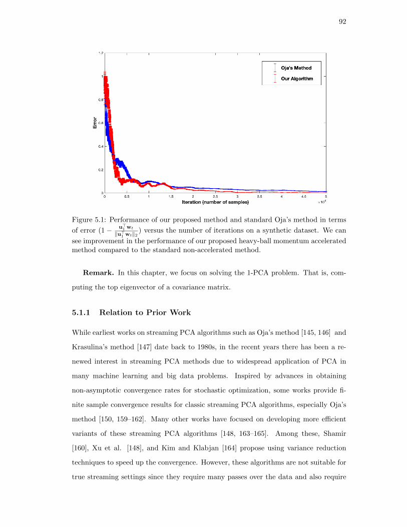
92

Figure 5.1: Performance of our proposed method and standard Oja’s method in terms

of error (1 − u>1 wt‖u>1 wt‖2

) versus the number of iterations on a synthetic dataset. We can

see improvement in the performance of our proposed heavy-ball momentum acceleratedmethod compared to the standard non-accelerated method.

Remark. In this chapter, we focus on solving the 1-PCA problem. That is, com-

puting the top eigenvector of a covariance matrix.


While earliest works on streaming PCA algorithms such as Oja’s method [145, 146] and

Krasulina’s method [147] date back to 1980s, in the recent years there has been a re-

newed interest in streaming PCA methods due to widespread application of PCA in

many machine learning and big data problems. Inspired by advances in obtaining

non-asymptotic convergence rates for stochastic optimization, some works provide fi-

nite sample convergence results for classic streaming PCA algorithms, especially Oja’s

method [150, 159–162]. Many other works have focused on developing more efficient

variants of these streaming PCA algorithms [148, 163–165]. Among these, Shamir

[160], Xu et al. [148], and Kim and Klabjan [164] propose using variance reduction

techniques to speed up the convergence. However, these algorithms are not suitable for

true streaming settings since they require many passes over the data and also require

93

O(d2) memory compared to O(d) memory cost of stochastic PCA methods without

variance reduction. Moreover, Xu et al. [148], and Kim and Klabjan [164] , similar to

our work, propose employing momentum-based acceleration to design stochastic PCA

algorithms.

While the efficacy of acceleration methods such as Polyak’s heavy ball method

[158, 166] and Nesterov’s accelerated gradient method [167] is well understood for de-

terministic (strongly) convex optimization problems, recently there has been a surge

in interest in analyzing accelerated stochastic algorithms due to their scalability and

their good performance in practice both in convex and nonconvex settings, especially

in deep learning [155, 168–170]. Notably, Aybat et al. [155], Can et al. [170], and

Jain et al. [154] study accelerated methods for strongly convex and certain classes of

convex problems, while some other works [171–173] focus their attention to analyzing

accelerated stochastic methods for nonconvex problems under mild conditions . While

PCA is a nonconvex problem, the aforementioned results on nonconvex optimization

only provide rates for first order convergence (convergence to a stationary point of the

objective function) and not necessarily global convergence rates. In the 1-PCA problem

which is the focus of this chapter, we are interested in finding the top eigenvector of

the matrix which corresponds to global optima of Problem 5.2.

The idea of employing acceleration methods to speed up PCA algorithms has been

proposed by Xu et al. [148], and Kim and Klabjan [164]. The proposed algorithms in

these works however require working with large mini-batches or multiple passes over

the data, making them undesirable for streaming settings. In contrast, we propose a

heavy ball accelerated variant of Oja’s method with multistage scheme for choosing the

step size that is suitable for streaming settings since only requires access to a single

data point per iteration. The multistage scheme for step size is adopted from Aybat et

al. [155], where they show that heavy ball accelerated SGD with a similar multistage

stepsize scheme achieves optimal convergence rate when applied to strongly convex,

smooth functions.

94


5.2.1 Notation and Definitions

Throughout this write-up, scalars are represented by lower case letters: a, and vec-

tors are denoted by boldface lower case letters: a. Boldface upper case letters denote

matrices: A and tensors are represented by boldface underlined upper case letters A.

We denote by ‖v‖p the `p norm of vector v (we abuse the terminology in case of

p = 0), while we use ‖A‖2, ‖A‖F , and ‖A‖tr to denote the spectral, Frobenius, and

trace (nuclear) norms of matrix A, respectively.

We denote by A⊗B ∈ Rm1m2×p1p2 the Kronecker product of matrices A ∈ Rm1×p1

and B ∈ Rm2×p2 . We use⊗N

n=1 An , A1 ⊗A2 ⊗ · · · ⊗AN for the Kronecker product

of N matrices. We drop the range indicators when there is no ambiguity.

5.2.2 The stochastic PCA problem

In streaming PCA, we want to find the top eigenvalue of a matrix Σ, given a sequence

of random samples At of Σ which are given to us in an online fashion. Here, we assume

that the streaming algorithms have access to a stochastic oracle that provides (noisy

unbiased) i.i.d. estimates At of a matrix Σ such that

E [At] = Σ, ‖At‖F ≤ r, E[‖At −Σ‖2F

]= σ2. (5.4)

A special (and common) case of this setting is estimating the covariance matrix Σ by

estimates At = xtxTt where xt is the random data sample presented to the algorithm

at time t.

Further, we assume that the largest eigenvalue of Σ is strictly greater than the

second largest eigenvalue, i.e., λ1 > λ2 ≥ λ3 ≥ · · ·λd.

95

5.2.3 Baseline Stochastic PCA Algorithms

The oldest and most well-known stochastic PCA algorithms are Oja’s method [145,

146] and Krasulina’s method [147]. In Oja’s method, the update rule is

w′t = (I + ηAt)wt−1, wt = w′t/‖w′t‖, (5.5)

which is sometimes written as

w′t =wt−1 + ηtAtwt−1

‖wt−1 + ηtAtwt−1‖, wt = w′t/‖w′t‖, (5.6)

On the other hand, the update rule in Krasulina’s algorithm is

wt = wt−1 + ηt

(At −

w>t−1Atwt−1

‖wt−1‖2I)wt−1. (5.7)

In this work, we focus on Oja’s rule and its variants.

5.2.4 Momentum-based Acceleration of Gradient-based Optimization

Methods

The baseline algorithm for solving a minimization problem with continuously differen-

tiable objective function f is the gradient descent (GD) method with update rule

wt = wt−1 − ηt∇f(wt−1), (5.8)

where ηt is the stepsize (also known as learning rate in the machine learning community).

The convergence rate of GD for convex functions with L-Lipschitz gradient is O(L/ε)

and when the function is also µ-strongly convex, it is O(L/µ log(1/ε)

)[157].

To improve the convergence of GD, accelerated first-order methods combine gradient

information at the current and the past iterate, as well as the iterates themselves. Most

common acceleration methods are Polyak’s heavy ball momentum method [158, 166]

and Nesterov’s accelerated gradient method [167].

Polyak’s method involves adding a “heavy-ball momentum” term β(wt−1 −wt−2).

96

The update rule in the heavy ball accelerated GD is

wt = wt−1 + β(wt−1 −wt−2)− ηt∇f(wt−1), (5.9)

which sometimes is written in form of

vt = β′vt−1 −∇f(wt−1)

wt = wt−1 + ηvt, (5.10)

where β′ = β′

ηt. On the other hand, Nesterov [167] proposed a slightly different momen-

tum method:

vt = β′vt−1 −∇wf(wt−1 + ηβ′vt−1)

wt = wt−1 + ηvt, (5.11)

which can also be written as

wt = wt−1 + β(wt−1 −wt−2)− η∇wf(wt−1 + β(wt−1 −wt−2)). (5.12)

The heavy ball method has been shown to have O(√

L/µ log(1/ε))

convergence rate

when the objective function f is twice continuously differentiable, strongly convex and

has Lipschitz continuous gradients, which is faster than both GD and Nesterov’s ac-

celerated gradient [157, 174]. However, the convergence of the heavy balling method

is not as well-established when f is not necessarily twice differentiable [174, 175]. On

the other hand, Nesterov’s method has improved convergence rate for both classes of

convex and strongly convex objective functions with Lipschitz continuous gradients.

Especially, in the case of convex optimization problems with Lipschitz continuous gra-

dients, Nesterov’s method acheives the optimal rate of O(√L/ε) [167, 174].

97

5.3 Oja’s Rule with Heavy Ball Acceleration with Fixed Step Size

In this section we study the convergence of Oja’s update rule with fixed step size and

Polyak’s heavy ball (HB) acceleration in the stochastic (streaming) setting. Consider

the following variant of the Oja’s rule:

w′t = (I + ηAt)wt−1 − βwt−2, wt = w′t/‖w′t‖, (5.13)

where At is the stochastic update at time t. We call this update rule the heavy ball

accelerated Oja’s Rule (HBOR), since the term −βwt−2 in the update works in similar

way to the heavy ball momentum term.

Define random matrices Ft such that w′t = Ftw0. Then (5.13) can be rewritten as

a matrix recursion for t ≥ 1:

Ft = (I + ηAt)Ft−1 − βFt−2, F0 = I, F−1 = 0. (5.14)

We can write update rule (5.13) in the compact form ξ′t = Mtξt−1 where

Mt ,

I + ηAt −βI

I 0

, (5.15)

and ξt =

wt

wt−1

and ξ′t =

w′t

w′t−1

. Since w′t = Ftw0, one can write Ft =

ZTMt · · ·M1Z, where Z ,

Id0d

.

Using the definition of Ft we have an expression for the residual error from projecting

98

the iterate on the top eigenvector:

1− 〈u1,w′t〉

2

‖w′t‖2= 1− (uT1 Ftw0)2

‖Ftw0‖2

=

∑di=2(uTi Ftw0)2∑di=1(uTi Ftw0)2

≤∑d

i=2(uTi Ftw0)2

(uT1 Ftw0)2. (5.16)

Thus, in order to find the convergence rate of the sequence generated by HBOR in

(5.13), we first bound E[∑d

i=2(uTi Ftw0)2]

and use Markov’s inequality to obtain a

high-probability upper bound on the numerator. For the denominator, we bound

Var(uT1 Ftw0) which yields a lower bound on |uT1 Ftw0| (and consequently (uT1 Ftw0)2)

using Chebyshev’s inequality.

To establish an error bound of HB-Oja’s rule with constant step size, we will first

introduce a series of lemmata that are essential in obtaining our results.

Lemma 17. Consider the update rule (5.13) and Ft defined in (5.14). Assume that

‖w0‖ = 1. Then,

‖E [Ft ⊗ Ft]− E [Ft]⊗ E [Ft] ‖ ≤ p2t (λ1)

(exp

[ σ2η2t

(1 + ηλ1)2 − 4β

]− 1), (5.17)

where σ2 = E[‖A−At‖2

], λ1 is the largest eigenvalue of matrix A, and the polynomial

sequence pt(x) is defined as

pt(x) = (1 + ηx)pt−1(x)− βpt−2(x), p1(x) = 1 + ηx, p0(x) = 1. (5.18)

Proof. We have Ft = ZTMt · · ·M1Z. Therefore,

E [Ft ⊗ Ft] = (Z⊗ Z)TE [Mt ⊗Mt] · · ·E [M1 ⊗M1] (Z⊗ Z)

= (Z⊗ Z)TE [Mt ⊗Mt]t (Z⊗ Z). (5.19)

We have Mt = M +

η(At −A) 0

0 0

. Define Mt , M −Mt. Since E[Mt

]= 0, we

99

have

E [Mt ⊗Mt]t = E

[(M− Mt)⊗ (M− Mt)

]t= (M⊗M + Σ)t, (5.20)

where Σ , E[Mt ⊗ Mt

]. It is clear that

Σ = E[(Zη(At −A)ZT )⊗ (Zη(At −A)ZT )

]= η2(Z⊗ Z)ΣA(Z⊗ Z)T ,

where ΣA , E [(At −A)⊗ (At −A)]. Now, we know from the binomial expansion of

matrices [148] that

(A + B)t =t∑

n=0

∑k∈Sn+1

t−n

Ak1

n+1∏i=2

BAki ,

where Sji , (k1, · · · , kj) ∈ Nj | k1 + · · ·+kj = i. Applying this expansion to the right

hand side of (5.20) results in

(M⊗M + Σ)t =

t∑n=0

∑k∈Sn+1

t−n

(M⊗M)k1

n+1∏i=2

Σ(M⊗M)ki

= (M⊗M)t +

t∑n=1

∑k∈Sn+1

t−n

(M⊗M)k1

n+1∏i=2

Σ(M⊗M)ki .

Since E [Ft] = E[ZTMt · · ·M1Z

]= ZTMtZ and consequently E [Ft] ⊗ E [Ft] = (Z ⊗

100

Z)T (M⊗M)t(Z⊗ Z), it follows that

‖E [Ft ⊗ Ft]− E [Ft]⊗ E [Ft] ‖

= ‖(Z⊗ Z)Tt∑

n=1

∑k

[(M⊗M)k1

n+1∏i=2

Σ(M⊗M)ki

](Z⊗ Z)‖

= ‖t∑

n=1

∑k

(Z⊗ Z)T

[(M⊗M)k1

n+1∏i=2

η2(Z⊗ Z) ·ΣA · (Z⊗ Z)T (M⊗M)ki

](Z⊗ Z)‖

= ‖t∑

n=1

∑k

(Z⊗ Z)T (M⊗M)k1(Z⊗ Z)

n+1∏i=2

[η2ΣA(Z⊗ Z)T (M⊗M)ki(Z⊗ Z)

]‖

= ‖t∑

n=1

∑k

(E [Fk1 ]⊗ E [Fk1 ])n+1∏i=2

[η2ΣA(E [Fki ]⊗ E [Fki ])

]‖

≤t∑

n=1

∑k

‖(E [Fk1 ]⊗ E [Fk1 ])n+1∏i=2

[η2ΣA(E [Fki ]⊗ E [Fki ])

]‖

≤t∑

n=1

∑k∈Sn+1

t−n

‖E [Fk1 ]⊗ E [Fk1 ] ‖2 · ‖n+1∏i=2

η2‖ΣA‖2 · ‖E [Fki ]⊗ E [Fki ] ‖2

≤t∑

n=1

‖η2ΣA‖n∑

k∈Sn+1t−n

‖E [Fk1 ]⊗ E [Fk1 ] ‖2n+1∏i=2

‖E [Fki ]⊗ E [Fki ] ‖2

=

t∑n=1

‖η2ΣA‖n∑

k∈Sn+1t−n

n+1∏i=1

‖E [Fki ]⊗ E [Fki ] ‖2. (5.21)

Now, using the properties of the polynomial sequence pt(x) described by (5.18) and the

101

fact that ‖E [Fki ] ‖2 = ‖pki(A)‖2 = pki(λ1), we get

‖E [Ft ⊗ Ft]− E [Ft]⊗ E [Ft] ‖

≤t∑

n=1

‖η2ΣA‖n∑

k∈Sn+1t−n

n+1∏i=1

‖E [Fki ] ‖22

=t∑

n=1

η2n‖ΣA‖n∑

k∈Sn+1t−n

n+1∏i=1

p2ki

(λ1)

(a)

≤t∑

n=1

η2n‖ΣA‖n∑

k∈Sn+1t−n

1

((1 + ηλ1)2 − 4β)np2n+

∑n+1i=1 ki

(λ1)

(b)= p2

t (λ1)

t∑n=1

η2n‖ΣA‖n t

t− n

1

((1 + ηλ1)2 − 4β)n

= p2t (λ1)

t∑n=1

t

t− n

( η2‖ΣA‖(1 + ηλ1)2 − 4β

)n(c)= p2

t (λ1)([ η2‖ΣA‖

(1 + ηλ1)2 − 4β+ 1]t− 1)

(d)

≤ p2t (λ1)

(exp

[ η2‖ΣA‖t(1 + ηλ1)2 − 4β

]− 1), (5.22)

where (a) follows from Corollary 4 in the Appendix (Section 6.2), (b) follows from

|Sn+1t−n | =

t

t− n

, (c) follows from the binomial theorem [148], and (d) follows from

1 + x ≤ exp(x). Finally, since ||ΣA|| = E[‖A−At‖2

]= σ2, we have

‖E [Ft ⊗ Ft]− E [Ft]⊗ E [Ft] ‖ ≤ p2t (λ1)

(exp

[ σ2η2t

(1 + ηλ1)2 − 4β

]− 1). (5.23)

The following lemma provides a high probability upper bound on the numerator of

the right hand side of inequality (5.16), i.e.,∑d

i=2(uTi Ftw0)2.


102

‖w0‖ = 1. Then, with probability at least 1− δ,

d∑i=2

(uTi Ftw0)2 ≤ 1

δ

[√d p2

t (λ1)(

exp[ σ2η2t

(1 + ηλ1)2 − 4β

]− 1)

+ p2t (λ2)(1− |uT1 w0|2)

].

(5.24)

Proof of Lemma 18. To find an upper bound on the numerator∑d

i=2(uTi Ftw0)2, we

use Markov’s inequality [45, 141]. To avoid complications of finding the exact value of

E[∑d

i=2(uTi Ftw0)2], we resort to finding an upper bound on it. We have

E

[d∑i=2

(uTi Ftw0)2

]

=d∑i=2

(E[(uTi Ftw0)2

]− E

[uTi Ftw0

]2) +

d∑i=2

E[uTi Ftw0

]2≤

d∑i=1

(E[(uTi Ftw0)2

]− E

[uTi Ftw0

]2) +

d∑i=2

E[uTi Ftw0

]2=

d∑i=1

(E[(uTi Ftw0)⊗ (uTi Ftw0)

]− E

[uTi Ftw0

]⊗ E

[uTi Ftw0

]) +

d∑i=2

E[uTi Ftw0

]2=

d∑i=1

(ui ⊗ ui)T (E [Ft ⊗ Ft]− E [Ft]⊗ E [Ft])(w0 ⊗w0) +

d∑i=2

E[uTi Ftw0

]2(a)

≤

∥∥∥∥∥d∑i=1

(ui ⊗ ui)

∥∥∥∥∥ · ‖E [Ft ⊗ Ft]− E [Ft]⊗ E [Ft]‖ · ‖w0 ⊗w0‖+d∑i=2

(pt(λi)uTi w0)2

≤√d p2

t (λ1)(

exp[ σ2η2t

(1 + ηλ1)2 − 4β

]− 1)

+ p2t (λ2)

d∑i=2

(uTi w0)2

(b)=√d p2

t (λ1)(

exp[ σ2η2t

(1 + ηλ1)2 − 4β

]− 1)

+ p2t (λ2)(1− |uT1 w0|2) (5.25)

where (a) follows from Cauchy–Schwarz inequality, (b) follows from orthonormality of

ui’s as basis vector. Using Markov’s inequality, we have that with probability at least

1− δ,

d∑i=2

(uTi Ftw0)2 ≤ 1

δ

[√d p2

t (λ1)(

exp[ σ2η2t

(1 + ηλ1)2 − 4β

]− 1)

+ p2t (λ2)(1− |uT1 w0|2)

]

for any fixed 0 < δ < 1.

103

Next, the following lemma provides a high probability lower bound on the denomi-

nator of the right hand side of inequality (5.16), i.e., (uT1 Ftw0)2.


‖w0‖ = 1. Then, with probability at least 1− δ we have

(uT1 Ftw0)2 ≥ p2t (λ1)

|uT1 w0| −

√exp

[ σ2η2t(1+ηλ1)2−4β

]− 1

δ

2

. (5.26)

Proof of Lemma 19. We use Chebyshev’s inequality [45, 141, 176] to find a lower bound

on the value of (uT1 Ftw0)2. The variance of the denominator Var(uT1 Ftw0) thus is

bounded as follows.

Var(uT1 Ftw0) = E[(uT1 Ftw0)2

]− (E

[(uT1 Ftw0)

])2

= E[(uT1 Ftw0)⊗ (uT1 Ftw0)

]− E

[(uT1 Ftw0)

]⊗ E

[(uT1 Ftw0)

]= (u1 ⊗ u1)T (E [Ft ⊗ Ft]− E [Ft]⊗ E [Ft])(w0 ⊗w0)

≤ ‖u1 ⊗ u1‖ · ‖E [Ft ⊗ Ft]− E [Ft]⊗ E [Ft] ‖ · ‖w0 ⊗w0‖

≤ p2t (λ1)

(exp

[ σ2η2t

(1 + ηλ1)2 − 4β

]− 1). (5.27)

Using Chebyshev’s inequality we get

P

|uT1 Ftw0 − uT1 pt(A)w0| ≥ pt(λ1)

√exp

[ σ2η2t(1+ηλ1)2−4β

]− 1

√δ

≤ δ.Note that

uTi pt(A) = uTi pt(λi)uiuTi = pt(λi)u

Ti . (5.28)

Therefore, we have

P

|uT1 Ftw0 − pt(λ1)uT1 w0| ≥ pt(λ1)

√exp

[ σ2η2t(1+ηλ1)2−4β

]− 1

√δ

≤ δ. (5.29)

104

Thus,

P

|uT1 Ftw0| ≤ pt(λ1)|uT1 w0| − pt(λ1)

√exp

[ σ2η2t(1+ηλ1)2−4β

]− 1

√δ

≤ δ (5.30)

and consequently

P

(uT1 Ftw0)2 ≤ p2t (λ1)

|uT1 w0| −

√exp

[ σ2η2t(1+ηλ1)2−4β

]− 1

δ

2 ≤ δ. (5.31)

Next, we investigate the termp2t (λ2)

p2t (λ1)

that will appear in the upper bound on the

error. The following lemma states the result.

Lemma 20. Given the polynomial sequence pt(x) defined as

pt(x) = (1 + ηx)pt−1(x)− βpt−2(x), p1(x) = 1 + ηx, p0(x) = 1,

and β = (1 + ηλ2)2/4, we have

p2t (λ2)

p2t (λ1)

≤( t+ 1∑t

n=0 a−2n

)2exp

(− 2t

√η∆√

1 + ηλ2

), (5.32)

where a ,µ1+

µ2=

(1+ηλ1)+√

(1+ηλ1)2−(1+ηλ2)2

1+ηλ2and ∆ = λ1 − λ2.

Proof of Lemma 20. It follows from Lemma 22 that when y , 1 + ηx is such that

y2 6= 4β, we have

pt(x) =1√

y2 − 4β

(y +√y2 − 4β

2

)t+1

−

(y −

√y2 − 4β

2

)t+1 ,

and when y2 = 4β, we have

pt(x) = (t+ 1)(√β)t. (5.33)

105

Plugging in our choice of β = (1 + ηλ2)2/4 results in

pt(λ1) =

((1+ηλ1)+

√(1+ηλ1)2−(1+ηλ2)2

2

)t+1−(

(1+ηλ1)−√

(1+ηλ1)2−(1+ηλ2)2

2

)t+1

√(1 + ηλ1)2 − (1 + ηλ2)2

=µt+1

1+− µt+1

1−

µ1+ − µ1−(5.34)

and

pt(λ2) = (t+ 1)((1 + ηλ2)/2)t = (t+ 1)(µ2

2

)t. (5.35)

pt(λ2)

pt(λ1)=

(µ1+ − µ1−)(t+ 1)µt2µt+1

1+− µt+1

1−

=(µ1+ − µ1−)(t+ 1)µt2

(µ1+ − µ1−)∑t

n=0 µt−n1+

µn1−. (5.36)

Since µ1+µ1− = (1 + ηλ2)2/4 = µ22, we have

µ1+

µ2= µ2

µ1−. Define a ,

µ1+

µ2. We have

pt(λ2)

pt(λ1)= (t+ 1)

µt2∑tn=0 µ

t−n1+

µn1−

= (t+ 1)µt2∑t

n=0 at−nµt−n2 a−nµn2

= (t+ 1)1∑t

n=0 at−n( 1

a)n

= (t+ 1)1

at∑t

n=0 a−2n

. (5.37)

Now, by showing that∑t

n=0 at−2n attains its minimum over a ≥ 1 at a = 1, we show

that pt(λ2)pt(λ1) < 1 for all t. We have

∂

∂a

t∑n=0

at−2n =t∑

n=0

(t− 2n)at−2n−1

=

bt/2c∑n=0

(t− 2n)at−2n−1 +t∑

n=bt/2c+1

(t− 2n)at−2n−1. (5.38)

106

It is clear that the first term has non-negative multiplier and exponent while the second

term has non-positive multiplier and exponent which make both terms increasing in a

for a ≥ 1. Since ∂∂a

∑tn=0 a

t−2n = 0 for a = 1, we have ∂∂a

∑tn=0 a

t−2n ≥ 1 for a > 1

which means∑t

n=0 at−2n > t+ 1 for all t and a > 1. Therefore,

pt(λ2)

pt(λ1)= (t+ 1)

1

at∑t

n=0 a−2n

=t+ 1∑tn=0 a

−2n(µ2

µ1+

)t < 1. (5.39)

We further have

( µ2

µ1+

)2t= exp

(2t log(|

µ2+

µ1+

|))

= exp

(2t log(

√4β

(1 + ηλ1) +√

(1 + ηλ1)2 − 4β)

)(1)= exp

(2t log(

1 + ηλ2

(1 + ηλ2) + η(λ1 − λ2) +√

(1 + ηλ1)2 − (1 + ηλ2)2)

)

≤ exp

(−2t log(1 +

η(λ1 − λ2) +√

(1 + ηλ1)2 − (1 + ηλ2)2

1 + ηλ2)

)(2)

≤ exp

(−2t

η(λ1 − λ2) +√

(1 + ηλ1)2 − (1 + ηλ2)2

1 + ηλ2

)

= exp

(−2t

η(λ1 − λ2) +√

(1 + ηλ1) + (1 + ηλ2)√

(1 + ηλ1)− (1 + ηλ2)

1 + ηλ2

)

= exp

(−2t

η(λ1 − λ2) +√

(1 + ηλ1) + (1 + ηλ2)√η(λ1 − λ2)

1 + ηλ2

)

= exp

(−2t

√1 + ηλ2

√η(λ1 − λ2)

1 + ηλ2

)exp

(−2t

η(λ1 − λ2)

1 + ηλ2

)≤ exp

(−2t

√η∆√

1 + ηλ2

), (5.40)

where ∆ = λ1 − λ is the eigengap of matrix A. Hence, we have

p2t (λ2)

p2t (λ1)

≤( t+ 1∑t

n=0 a−2n

)2exp

(− 2t

√η∆√

1 + ηλ2

). (5.41)

Now we are ready to provide an error bound on HBOR with constant step size.

107

Theorem 9 states this result.

Theorem 9. Consider a PSD matrix A ∈ Rd×d with eigenvalues 1 ≥ λ1 ≥ · · · ≥ λd

and eigengap ∆ := λ1 − λ2. Assume that estimates At of matrix A satisfy the set

of assumptions in (5.4). Consider the estimates wt generated by the accelerated Oja’s

method with heavy-balling

w′t = (I + ηAt)wt−1 − βwt−2, wt = w′t/‖w′t‖,

with β = (1 + ηλ2)2/4 and constant stepsize η. Suppose that for some ι > 0 we have

ησ2 <(2+η(λ1+λ2))·∆·(|uT1 w0|−

√ι)2

T . Then, with probability at least 1− 2δ, we have

eT , 1−〈u1,w

′T 〉

2

‖w′T ‖2≤ K1ηT +K2e0

( T + 1∑Tt=0 a

−2t

)2e−γ√ηT , (5.42)

where K1 =√d2σ2

δ(2+η(λ1+λ2))∆ι , K2 = 1δι , a =

(1+ηλ1)+√

(1+ηλ1)2−(1+ηλ2)2

1+ηλ2, and γ =

2√

∆√1+ηλ2

.

Proof of Theorem 9. We want a high probability upper bound on (5.16) to get an upper

bound on 1 − 〈u1,w′t〉2

‖w′t‖2. We saw in inequality (5.16) that 1 − 〈u1,w′t〉

2

‖w′t‖2≤

∑di=2(uTi Ftw0)2

(uT1 Ftw0)2 .

Now, we find a high probability upper bound on the numerator of the right hand side,∑di=2(uTi Ftw0)2, and a high probability lower bound on the denominator, (uT1 Ftw0)2.

We showed in Lemma 18 that with probability at least 1− δ,

d∑i=2

(uTi Ftw0)2 ≤ 1

δ

[√d p2

t (λ1)(

exp[ σ2η2t

(1 + ηλ1)2 − 4β

]− 1)

+ p2t (λ2)(1− |uT1 w0|2)

].

Furthermore, we showed in Lemma 19 that with probability not less than 1− δ,

(uT1 Ftw0)2 ≥ p2t (λ1)

|uT1 w0| −

√exp

[ σ2η2t(1+ηλ1)2−4β

]− 1

δ

2

.

108

It follows from these results, using a union bound, that with probability at least 1−2δ,

∑di=2(uTi Ftw0)2

(uT1 Ftw0)2≥

√d p2

t (λ1)(

exp[

σ2η2t(1+ηλ1)2−4β

]− 1)

+ p2t (λ2)(1− |uT1 w0|2)

δp2t (λ1)

[|uT1 w0| −

√(exp

[ σ2η2t(1+ηλ1)2−4β

]− 1)/δ

]2 . (5.43)

Plugging in β = (1 + ηλ2)2/4, we get with probability at least 1− 2δ,

∑di=2(uTi Ftw0)2

(uT1 Ftw0)2≥

√d(

exp[ σ2ηt

(2+η(λ1+λ2))∆

]− 1)

δ[|uT1 w0| −

√exp[

σ2ηt(2+η(λ1+λ2))∆

]−1

δ

]2

+p2t (λ2)(1− |uT1 w0|2)

δp2t (λ1)

[|uT1 w0| −

√exp[

σ2ηt(2+η(λ1+λ2))∆

]−1

δ

]2 .(5.44)

If we have ησ2 < (2+η(λ1+λ2))∆t , then we have exp

(σ2ηt

(2+η(λ1+λ2))∆

)− 1 ≤ 2σ2ηt

(2+η(λ1+λ2))∆

and also exp(

σ2ηt(2+η(λ1+λ2))∆

)− 1 ≥ σ2ηt

(2+η(λ1+λ2))∆ . Therefore, with probability at least

1− 2δ,

1− 〈u1,w′t〉

2

‖w′t‖2≤

√d2σ2ηt

δ(2 + η(λ1 + λ2))∆[|uT1 w0| −

√σ2ηt

δ(2+η(λ1+λ2))∆

]2 +

(1− |uT1 w0|2)

δ[|uT1 w0| −

√σ2ηt

δ(2+η(λ1+λ2))∆

]2

p2t (λ2)

p2t (λ1)

. (5.45)

Furthermore, if we have ησ2 <(2+η(λ1+λ2))·∆·(|uT1 w0|−

√ι)2

t for some ι > 0, then we have

[|uT1 w0| −

√σ2ηt

δ(2 + η(λ1 + λ2))∆

]2

> ι. (5.46)

Therefore, we have

1− 〈u1,w′t〉

2

‖w′t‖2≤

√d2σ2ηt

δ(2 + η(λ1 + λ2))∆ι+

(1− |uT1 w0|2)

δι

p2t (λ2)

p2t (λ1)

. (5.47)

plugging the bound onp2t (λ2)

p2t (λ1)

in Lemma 20 into (5.47) results in the bound in the

statement of Theorem 9.

109

Next, we show that if we know the iteration budget ahead of time, we can choose a

fixed stepsize such that the HBOR algorithm obtains near optimal (up to polylog term)

decay in variance term (but non-optimal decay in bias term).

Corollary 2. Consider the setting of Theorem 9. Given a budget of T iterations, with

the choice of stepsize η = ( p log T√2∆T

)2 1λ1

, we have the following error after T > 2p√2∆

log p√2∆

iterations:

eT ≤9√dσ2

2∆2δι

log2 T

T+

e0

διT p′−2, (5.48)

where p′ = p√√λ1

.

Proof. It follows from Theorem 9 that

et ≤ K1ηT +K2e0T2e−γ

√ηT . (5.49)

It follows from T > 2p√2∆

log p√2∆

that p log T√2∆T

≤ 1. Furthermore, we have γ ≤√

2∆.

Then, we have

et ≤ K1ηT +K2e0T2e− p√

λ1log T

≤ K1p2 log2 T

2∆ · T1

λ1+K2e0T

2− p√λ1 .

By setting p = p′√λ1, we have

eT ≤9√dσ2

2∆2δι

log2 T

T+

e0

διT p′−2. (5.50)

5.4 Multistage HB Accelerated PCA

We showed in the last section that accelerated PCA with O( log2 TT 2 ) step-size results in

an extra ( log2 TT 2 ) rate for the bias term and ( log2 T

T 2 ). In this section, we follow the method

proposed in Aybat et al. [155] to break the optimization process into multiple stages

110

in hope of improving the convergence rate of accelerated PCA. This method, which we

call Multistage heavy ball-accelerated Oja’s rule (MHBOR), consists of successive runs

of HBOR with (different) fixed stepsizes. Specifically, the estimates are generated by

the following rule.

w′tk = (I + ηkAtk)wtk−1 − βkwtk−2, wtk = w′tk/‖w′tk‖.

where 1 ≤ tk ≤ Tk with

k = 1 : η1 = η ≤ 1

λ1, T1 ≥ 1,

k > 1 : ηk = η/22k, Tk = (1 + c)2kT , (1 + c)2kd 1

γk√η

log(K22p)e. (5.51)

and βk = (1 + ηkλ2)2/4 and c > 0.

Remark. The learning rate and the number of iterations are inspired by Aybat

et al. [155]. The (1 + c)2 term is intended to overcome the difficulty caused by the

(T + 1)2/∑T

t=0 a−2t term on the RHS of (5.42).

Before stating the convergence result of MHBOR, we present Lemma 21 that will

prove useful in establishing the convergence result. We know from Theorem 9 that in

the k-th stage of MHBOR, we have

ekT ≤ K1ηT +K2ek0

( T + 1∑Tt=0 a

−2t

)2e−γ√ηt, (5.52)

where ek0 is the error in the beginning of the the k-th stage and ekt is the the error after

t iterations in the k-th stage. In Lemma 21, we study how the term (T+1)2∑Tt=0 a

−2tlooks in

this scheme.

Lemma 21. Consider a PSD matrix A ∈ Rd×d with eigenvalues 1 ≥ λ1 ≥ · · · ≥ λd

and eigengap ∆ , λ1 − λ2. Assume that estimates At of matrix A satisfy the set

of assumptions in (5.4). Consider the estimates stepsize ηk and epoch length Tk as

described in (5.51). Suppose that we have ησ2 <(2+η(λ1+λ2))·∆·(|uT1 w0|−

√ι)2

T1for some

111

ι > 0. Define ak ,(1+ηkλ1)+

√(1+ηkλ1)2−(1+ηkλ2)2

1+ηkλ2. Then, we have

Tk∑Tk−1t=0 a−2t

k

≤ 16T . (5.53)

Proof of Lemma 21. In the multistage method, the values of η, and consequently the

values of µ2, µ1+ and a, change at every stage. At stage k, the value we have

ak =µ1+,k

µ2,k=

(1 + ηkλ1) +√

(1 + ηkλ1)2 − (1 + ηkλ2)2

1 + ηkλ2

=1 + ηλ1/2

2k +√η∆√

2 + η22k

(λ1 + λ2)/2k

1 + ηλ2/22k. (5.54)

Let us find a lower bound on

t∑n=0

a−2nk =

1− a−2(t+1)k

1− a−2k

.

Define τ , 22k for k > 1. We have

a−2k =

1 + ηλ1/τ2 +√η∆√

2 + ητ2 (λ1 + λ2)/τ

1 + ηλ2/τ2

−2

=

1 +η∆/τ2 +

√η∆√

2 + ητ2 (λ1 + λ2)/τ

1 + ηλ2/τ2

−2

≥(

1 +η∆/τ2 + 2

√η∆/τ

1 + ηλ2/τ2

)−2

≥(

1 +3√η∆/τ

1 + ηλ2/τ2

)−2

≥(

1 +3√η∆

τ

)−2

. (5.55)

112

Note that for K > 1, the final bound can be improved to(

1 + 2√η∆τ

)−2. Moreover,

a−2Tkk =

1 + ηλ1/τ2 +√η∆√

2 + ητ2 (λ1 + λ2)/τ

1 + ηλ2/τ2

−2Tk

=

1 +η∆/τ2 +

√η∆√

2 + ητ2 (λ1 + λ2)/τ

1 + ηλ2/τ2

−2Tk

≤(

1 +η∆/τ2 +

√2η∆/τ

2

)−2Tk

=1(

1 + η∆/τ2+√

2η∆/τ2

)2Tk

(a)

≤ 1

1 + η∆Tk/τ2 +√

2η∆Tk/τ, (5.56)

where (a) is due to Bernoulli’s inequality. Define u ,√η∆. For K = 1 we have

T1∑n=0

a−2n1 =

1− a−2(T1+1)1

1− a−21

≥1− 1

1+η∆T1+√

2η∆T1

1−(1 + 3

√η∆)−2

=

u2T1+√

2uT1

1+u2T1+√

2uT1

1− 1(1+3u)2

=

(u2 +

√2u)T1(1 + 3u)2(

1 + u2T1 +√

2uT1

)(6u+ 9u2)

≥ T1(1 + 3u)2

9(1 + u2T1 +

√2uT1

)≥ (1 + 3u)2

9(1 + u2 +

√2u)

≥ (1 + 3u)2

4 (1 + u)2

≥ 1

4, (5.57)

which is trivial since we know∑T1

n=0 a−2n1 > 1. However, for K > 1 the bound is

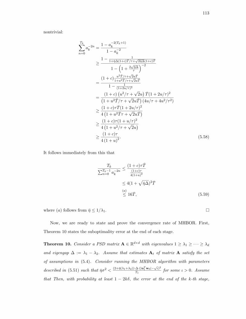
113

nontrivial:

Tk∑n=0

a−2nk =

1− a−2(Tk+1)k

1− a−2k

≥1− 1

1+η∆(1+c)T /τ+√

2η∆(1+c)T

1−(

1 + 2√η∆τ

)−2

=(1 + c) u2T /τ+

√2uT

1+u2T /τ+√

2uT

1− 1(1+2u/τ)2

=(1 + c)

(u2/τ +

√2u)T (1 + 2u/τ)2(

1 + u2T /τ +√

2uT)

(4u/τ + 4u2/τ2)

≥ (1 + c)τ T (1 + 2u/τ)2

4(1 + u2T τ +

√2uT

)≥ (1 + c)τ(1 + u/τ)2

4(1 + u2/τ +

√2u)

≥ (1 + c)τ

4 (1 + u)2 . (5.58)

It follows immediately from this that

Tk∑Tk−1n=0 a−2n

k

≤ (1 + c)τ T(1+c)τ

4(1+u)2

≤ 4(1 +√η∆)2T

(a)

≤ 16T , (5.59)

where (a) follows from η ≤ 1/λ1.

Now, we are ready to state and prove the convergence rate of MHBOR. First,

Theorem 10 states the suboptimality error at the end of each stage.


and eigengap ∆ := λ1 − λ2. Assume that estimates At of matrix A satisfy the set

of assumptions in (5.4). Consider running the MHBOR algorithm with parameters

described in (5.51) such that ησ2 <(2+η(λ1+λ2))·∆·(|uT1 w0|−

√ι)2

T1for some ι > 0. Assume

that Then, with probability at least 1 − 2kδ, the error at the end of the k-th stage,

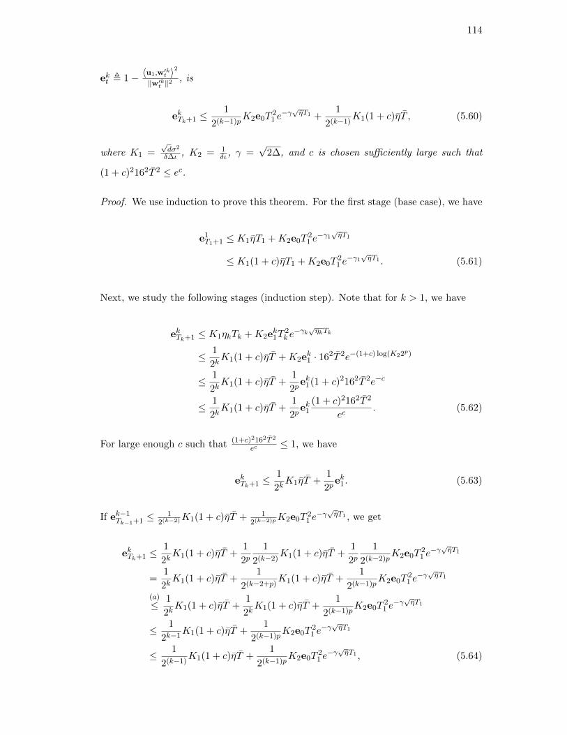
114

ekt , 1− 〈u1,w′kt 〉2‖w′kt ‖2

, is

ekTk+1 ≤1

2(k−1)pK2e0T

21 e−γ√ηT1 +

1

2(k−1)K1(1 + c)ηT , (5.60)

where K1 =√dσ2

δ∆ι , K2 = 1δι , γ =

√2∆, and c is chosen sufficiently large such that

(1 + c)2162T 2 ≤ ec.

Proof. We use induction to prove this theorem. For the first stage (base case), we have

e1T1+1 ≤ K1ηT1 +K2e0T

21 e−γ1√ηT1

≤ K1(1 + c)ηT1 +K2e0T21 e−γ1√ηT1 . (5.61)

Next, we study the following stages (induction step). Note that for k > 1, we have

ekTk+1 ≤ K1ηkTk +K2ek1T

2k e−γk√ηkTk

≤ 1

2kK1(1 + c)ηT +K2e

k1 · 162T 2e−(1+c) log(K22p)

≤ 1

2kK1(1 + c)ηT +

1

2pek1(1 + c)2162T 2e−c

≤ 1

2kK1(1 + c)ηT +

1

2pek1

(1 + c)2162T 2

ec. (5.62)

For large enough c such that (1+c)2162T 2

ec ≤ 1, we have

ekTk+1 ≤1

2kK1ηT +

1

2pek1. (5.63)

If ek−1Tk−1+1 ≤

12(k−2)K1(1 + c)ηT + 1

2(k−2)pK2e0T21 e−γ√ηT1 , we get

ekTk+1 ≤1

2kK1(1 + c)ηT +

1

2p1

2(k−2)K1(1 + c)ηT +

1

2p1

2(k−2)pK2e0T

21 e−γ√ηT1

=1

2kK1(1 + c)ηT +

1

2(k−2+p)K1(1 + c)ηT +

1

2(k−1)pK2e0T

21 e−γ√ηT1

(a)

≤ 1

2kK1(1 + c)ηT +

1

2kK1(1 + c)ηT +

1

2(k−1)pK2e0T

21 e−γ√ηT1

≤ 1

2k−1K1(1 + c)ηT +

1

2(k−1)pK2e0T

21 e−γ√ηT1

≤ 1

2(k−1)K1(1 + c)ηT +

1

2(k−1)pK2e0T

21 e−γ√ηT1 , (5.64)

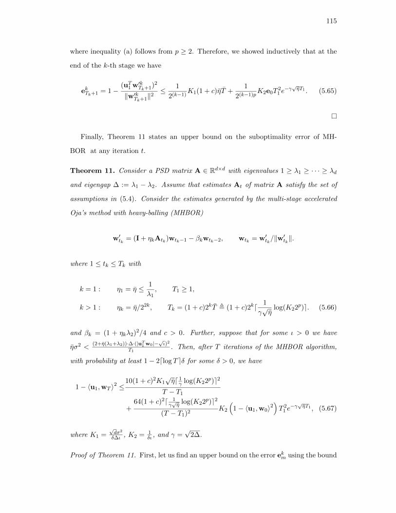
115

where inequality (a) follows from p ≥ 2. Therefore, we showed inductively that at the

end of the k-th stage we have

ekTk+1 = 1−(uT1 w′kTk+1)2

‖w′kTk+1‖2≤ 1

2(k−1)K1(1 + c)ηT +

1

2(k−1)pK2e0T

21 e−γ√ηT1 . (5.65)

Finally, Theorem 11 states an upper bound on the suboptimality error of MH-

BOR at any iteration t.


and eigengap ∆ := λ1 − λ2. Assume that estimates At of matrix A satisfy the set of

assumptions in (5.4). Consider the estimates generated by the multi-stage accelerated

Oja’s method with heavy-balling (MHBOR)

w′tk = (I + ηkAtk)wtk−1 − βkwtk−2, wtk = w′tk/‖w′tk‖.

where 1 ≤ tk ≤ Tk with

k = 1 : η1 = η ≤ 1

λ1, T1 ≥ 1,

k > 1 : ηk = η/22k, Tk = (1 + c)2kT , (1 + c)2kd 1

γ√η

log(K22p)e. (5.66)

and βk = (1 + ηkλ2)2/4 and c > 0. Further, suppose that for some ι > 0 we have

ησ2 <(2+η(λ1+λ2))·∆·(|uT1 w0|−

√ι)2

T1. Then, after T iterations of the MHBOR algorithm,

with probability at least 1− 2dlog T eδ for some δ > 0, we have

1− 〈u1,wT 〉2 ≤10(1 + c)2K1

√ηd 1

γ log(K22p)e2

T − T1

+64(1 + c)2d 1

γ√η

log(K22p)e2

(T − T1)2K2

(1− 〈u1,w0〉2

)T 2

1 e−γ√ηT1 , (5.67)

where K1 =√dσ2

δ∆ι , K2 = 1δι , and γ =

√2∆.

Proof of Theorem 11. First, let us find an upper bound on the error ekm using the bound

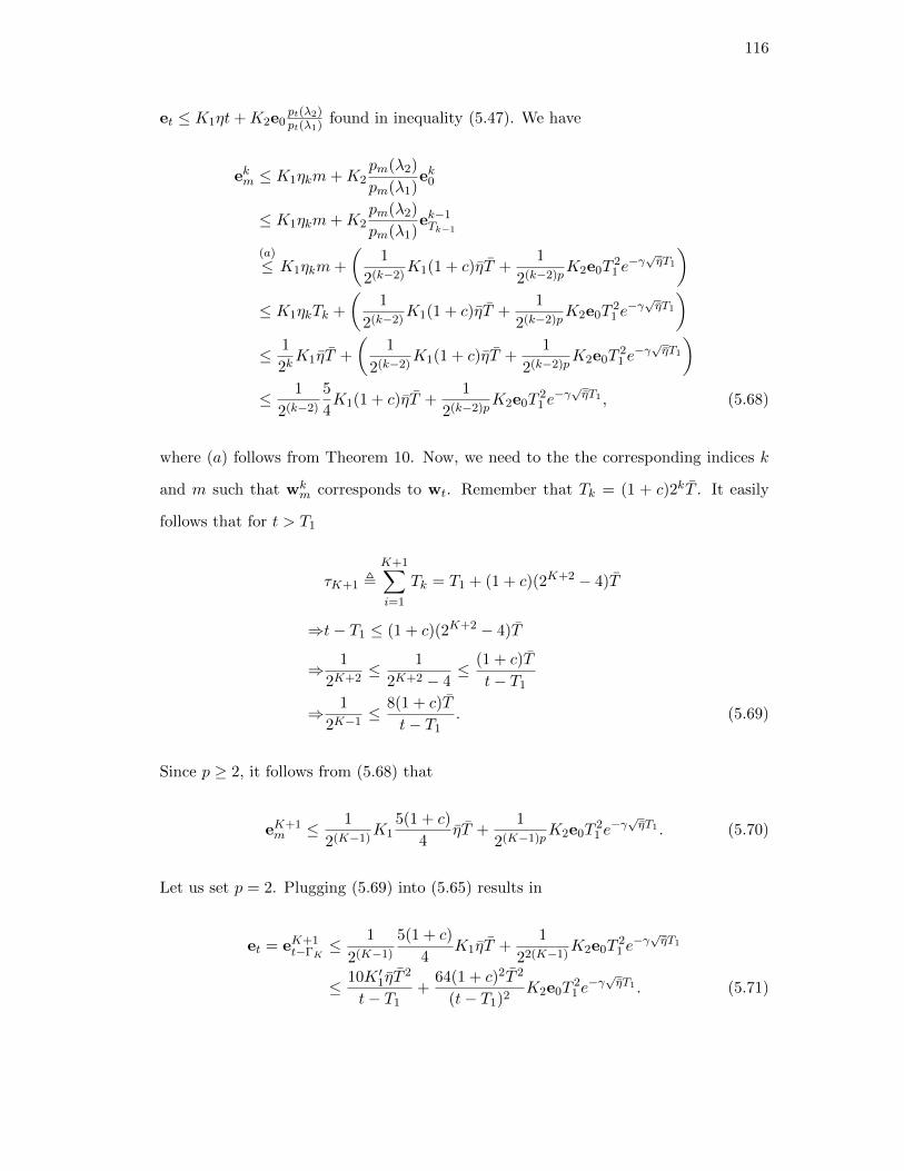
116

et ≤ K1ηt+K2e0pt(λ2)pt(λ1) found in inequality (5.47). We have

ekm ≤ K1ηkm+K2pm(λ2)

pm(λ1)ek0

≤ K1ηkm+K2pm(λ2)

pm(λ1)ek−1Tk−1

(a)

≤ K1ηkm+

(1

2(k−2)K1(1 + c)ηT +

1

2(k−2)pK2e0T

21 e−γ√ηT1

)≤ K1ηkTk +

(1

2(k−2)K1(1 + c)ηT +

1

2(k−2)pK2e0T

21 e−γ√ηT1

)≤ 1

2kK1ηT +

(1

2(k−2)K1(1 + c)ηT +

1

2(k−2)pK2e0T

21 e−γ√ηT1

)≤ 1

2(k−2)

5

4K1(1 + c)ηT +

1

2(k−2)pK2e0T

21 e−γ√ηT1 , (5.68)

where (a) follows from Theorem 10. Now, we need to the the corresponding indices k

and m such that wkm corresponds to wt. Remember that Tk = (1 + c)2kT . It easily

follows that for t > T1

τK+1 ,K+1∑i=1

Tk = T1 + (1 + c)(2K+2 − 4)T

⇒t− T1 ≤ (1 + c)(2K+2 − 4)T

⇒ 1

2K+2≤ 1

2K+2 − 4≤ (1 + c)T

t− T1

⇒ 1

2K−1≤ 8(1 + c)T

t− T1. (5.69)

Since p ≥ 2, it follows from (5.68) that

eK+1m ≤ 1

2(K−1)K1

5(1 + c)

4ηT +

1

2(K−1)pK2e0T

21 e−γ√ηT1 . (5.70)

Let us set p = 2. Plugging (5.69) into (5.65) results in

et = eK+1t−ΓK

≤ 1

2(K−1)

5(1 + c)

4K1ηT +

1

22(K−1)K2e0T

21 e−γ√ηT1

≤ 10K ′1ηT2

t− T1+

64(1 + c)2T 2

(t− T1)2K2e0T

21 e−γ√ηT1 . (5.71)

117

where K ′1 = (1 + c)2K1 and ΓK =∑K

k=1 Tk. Therefore, for t > T1 we have

1− 〈u1,wt〉2 ≤10K ′1

√ηd 1

γ log(K22p)e2

t− T1

+64(1 + c)2d 1

γ√η

log(K22p)e2

(t− T1)2K2

(1− 〈u1,w0〉2

)T 2

1 e−γ√ηT1 . (5.72)

In the following corollary of Theorem 11 we show that our algorithm, up to a

logarithmic factor, achieves the error upper bounds Ω( σ2

(λ1−λ2)2t) and Ω(e0e

−√λ1−λ2t)

for the noise term and the bias term, respectively.

Corollary 3. Consider the setting of Theorem 11. Suppose the computational budget

of T = αT1 for some α ≥ 2. Then with probability at least 1 − 2dlog T eδ, for eT ,

1− 〈u1,wT 〉2 we have

eT ≤ C1

√√dσ2ηdlog(K22p)e2

∆2T+ C2d

1√η∆

log(K22p)e2K2e0e−c√η∆T , (5.73)

where K2 = 1δι .

Remark. Note that the probability of the result in Theorem 11 holds with proba-

bility at least 1−2dlog T eδ. In order to boost the probability to 1−δ, is to run O(logT )

copies of the algorithm, each with 1 − 2dlog T eδ success probability and then output

the geometric median of the solutions, which can be done in nearly linear time [177].


In this chapter, we studied the problem of estimating the top eigenvector of the covari-

ance matrix of a multivariate random variable from i.i.d samples in a streaming setting.

A well-known and commonly used algorithm for solving this problem is called Oja’s

method which can be thought of as projected stochastic gradient descent (SGD). In-

spired by recent works on accelerating SGD for certain classes of convex problems [154–

157], we investigated the effect of applying a momentum-based acceleration method

118

called the heavy ball method (Polyak momentum) [158, 166] to Oja’s method.We pro-

posed a novel accelerated variant of Oja’s rule, called MHBOR, that employs a multi-

stage scheme for choosing the step size. We showed near-optimal convergence of this

multi-stage accelerated algorithm in the true streaming scheme without the need for

large mini-batches or variance reduction schemes, a property that distinguishes our

algorithm and our analysis from the existing works on accelerating Oja’s method.

We prove the convergence of this multi-stage algorithm and show that it approxi-

mately (up to a log factor) achieves the O( √

dσ2

(λ1−λ2)2t

)upper bound in the bias term and

O(e0e−√λ1−λ2t) upper bound in the noise term. When compared to the minimax lower

bounds Ω( σ2

(λ1−λ2)2t) and Ω(e0e

−√λ1−λ2t) for the noise term and the bias term respec-

tively, it becomes clear that our bounds for MHBOR are optimal up to a logarithmic

factor (as well as a√d factor in the noise term.)

While the dependence of our convergence result on dimensions d is not optimal

and there is an extra log factor in dependence on t, our results show that there could

be benefit in applying momentum acceleration to stochastic solvers in this structured

nonconvex problem.

In terms of future work, improving the analysis of the algorithm to potentially obtain

tighter convergence results is a possible direction. Moreover, Aybat et al. [155] show

that acceleration can improve robustness to gradient noise power of gradient methods

in stochastic settings (quantified in terms of asymptotic expected suboptimality of

the iterates), at least for certain classes of strongly convex function. Inspired by this

result, studying the robustness of the the accelerated and non-accelerated stochastic

PCA algorithms is another interesting future direction. For stochastic algorithms, in

addition to convergence rate, the robustness is an important criteria when comparing

performances of different algorithms.

119

Bibliography

[1] S. Bhojanapalli, B. Neyshabur, and N. Srebro, “Global optimality of local search

for low rank matrix recovery,” in Proc. Int. Conf. Advances Neural inf. Process.

Syst., 2016, pp. 3873–3881.

[2] D. Park, A. Kyrillidis, C. Carmanis, and S. Sanghavi, “Non-square matrix

sensing without spurious local minima via the Burer-Monteiro approach,” in

Proc. Int. Conf. Advances Neural Inf. Process. Syst., Apr. 2017, pp. 65–74.

[3] E. J. Candes and B. Recht, “Exact matrix completion via convex optimization,”

Found. Comput. Math., vol. 9, no. 6, p. 717, Apr. 2009.

[4] R. Sun and Z. Q. Luo, “Guaranteed matrix completion via non-convex factoriza-

tion,” IEEE Trans. Inf. Theory, vol. 62, no. 11, pp. 6535–6579, Nov. 2016.

[5] R. Ge, C. Jin, and Y. Zheng, “No spurious local minima in nonconvex low rank

problems: A unified geometric analysis,” in Proc. Int. Conf. Advances Neural inf.

Process. Syst., 2017, p. 1233–1242.

[6] E. J. Candes, X. Li, and M. Soltanolkotabi, “Phase retrieval via wirtinger flow:

Theory and algorithms,” IEEE Trans. Inf. Theory, vol. 61, no. 4, pp. 1985–2007,

Apr. 2015.

[7] P. Netrapalli, P. Jain, and S. Sanghavi, “Phase retrieval using alternating

minimization,” in Proc. Int. Conf. Advances Neural inf. Process. Syst., 2013, pp.

2796–2804.

[8] K. Kreutz-Delgado, J. F. Murray, B. D. Rao, K. Engan, T.-W. Lee, and T. J. Se-

jnowski, “Dictionary learning algorithms for sparse representation,” Neural Com-

put., vol. 15, no. 2, pp. 349–396, 2003.

120

[9] I. Tosic and P. Frossard, “Dictionary learning,” IEEE Signal Process. Mag.,

vol. 28, no. 2, pp. 27–38, Mar. 2011.

[10] G. H. Golub and C. F. Van Loan, “An analysis of the total least squares problem,”

SIAM J. Numer. Anal., vol. 17, no. 6, pp. 883–893, 1980.

[11] E. J. Candes, X. Li, Y. Ma, and J. Wright, “Robust principal component

analysis?” J. ACM, vol. 58, no. 3, pp. 11:1–11:37, May 2011.

[12] A. Ahmed, B. Recht, and J. Romberg, “Blind deconvolution using convex pro-

gramming,” IEEE Trans. Inf. Theory, vol. 60, no. 3, pp. 1711–1732, 2013.

[13] M. Aharon, M. Elad, and A. Bruckstein, “K-SVD: An algorithm for designing

overcomplete dictionaries for sparse representation,” IEEE Trans. Signal Process.,

vol. 54, no. 11, pp. 4311–4322, Nov. 2006.

[14] L. R. Tucker, “Implications of factor analysis of three-way matrices for measure-

ment of change,” Problems in Measuring Change, pp. 122–137, 1963.

[15] R. A. Harshman, “Foundations of the PARAFAC procedure: Models and con-

ditions for an explanatory multi-modal factor analysis,” UCLA Work. Papers

Phonetics, vol. 16, pp. 1–84, Dec. 1970.

[16] M. F. Duarte and R. G. Baraniuk, “Kronecker compressive sensing,” IEEE Trans.

Image Process., vol. 21, no. 2, pp. 494–504, 2011.

[17] Z. Shakeri, A. D. Sarwate, and W. U. Bajwa, “Identifiability of Kronecker-

structured dictionaries for tensor data,” IEEE J. Sel. Topics Signal Process.,

vol. 12, no. 5, pp. 1047 – 1062, 2018.

[18] N. Cressie and H.-C. Huang, “Classes of nonseparable, spatio-temporal stationary

covariance functions,” J. Amer. Statist. Assoc., vol. 94, no. 448, pp. 1330–1339,

1999.

[19] R. H. Keshavan, A. Montanari, and S. Oh, “Matrix completion from noisy

entries,” J. Mach. Learn. Res., vol. 11, pp. 2057–2078, 2010.

121

[20] Y. Koren, R. Bell, and C. Volinsky, “Matrix factorization techniques for recom-

mender systems,” Computer, vol. 42, no. 8, pp. 30–37, Aug. 2009.

[21] M. Signoretto, R. Van de Plas, B. De Moor, and J. A. K. Suykens, “Tensor versus

matrix completion: A comparison with application to spectral data,” IEEE Signal

Process. Lett., vol. 18, no. 7, pp. 403–406, 2011.

[22] B. Recht, “A simpler approach to matrix completion,” J. Mach. Learn. Res.,

vol. 12, no. Dec, pp. 3413–3430, 2011.

[23] E. J. Candes and T. Tao, “The power of convex relaxation: Near-optimal matrix

completion,” IEEE Trans. Inf. Theory, vol. 56, no. 5, pp. 2053–2080, May 2010.

[24] M. Xu, R. Jin, and Z.-H. Zhou, “Speedup matrix completion with side

information: Application to multi-label learning,” in Proc. Int. Conf. Advances

Neural inf. Process. Syst., 2013, pp. 2301–2309.

[25] K. Zhong, P. Jain, and I. S. Dhillon, “Efficient matrix sensing using rank-1

gaussian measurements,” in Proc. Int. Conf. Algorithmic Learn. Theory, 2015,

pp. 3–18.

[26] J. Lu, G. Liang, J. Sun, and J. Bi, “A sparse interactive model for matrix

completion with side information,” in Proc. Int. Conf. Advances Neural inf.

Process. Syst., 2016, pp. 4071–4079.

[27] K.-Y. Chiang, C.-J. Hsieh, and I. S. Dhillon, “Matrix completion with noisy side

information,” in Proc. Int. Conf. Advances Neural inf. Process. Syst., 2015, pp.

3447–3455.

[28] A. Soni, T. Chevalier, and S. Jain, “Noisy inductive matrix completion under

sparse factor models,” in IEEE Int. Symp. Inf. Theory, June 2017, pp. 2990–

2994.

[29] A. Eftekhari, D. Yang, and M. B. Wakin, “Weighted matrix completion and

recovery with prior subspace information,” IEEE Trans. Inf. Theory, vol. 64,

no. 6, pp. 4044–4071, 2018.

122

[30] N. Rao, H. Yu, P. Ravikumar, and I. S. Dhillon, “Collaborative filtering with

graph information: Consistency and scalable methods,” in Proc. Int. Conf.

Advances Neural inf. Process. Syst., 2015, pp. 2107–2115.

[31] B. Recht, M. Fazel, and P. A. Parrilo, “Guaranteed minimum-rank solutions of

linear matrix equations via nuclear norm minimization,” SIAM Rev., vol. 52,

no. 3, pp. 471–501, 2010.

[32] D. Gross, “Recovering low-rank matrices from few coefficients in any basis,” IEEE

Trans. Inf. Theory, vol. 57, no. 3, pp. 1548–1566, Mar. 2011.

[33] R. H. Keshavan, A. Montanari, and S. Oh, “Matrix completion from a few en-

tries,” IEEE Trans. Inf. Theory, vol. 56, no. 6, pp. 2980–2998, June 2010.

[34] P. Jain, P. Netrapalli, and S. Sanghavi, “Low-rank matrix completion using

alternating minimization,” in Proc. Annu. ACM Symp. Theory Comput., 2013,

pp. 665–674.

[35] J. Cai, E. J. Candes, and Z. Shen, “A singular value thresholding algorithm for

matrix completion,” SIAM J. Optimization, vol. 20, no. 4, pp. 1956–1982, 2010.

[36] K. Toh and S. Yun, “An accelerated proximal gradient algorithm for nuclear

norm regularized linear least squares problems,” Pacific J. Optimization, vol. 6,

pp. 615–640, 2010.

[37] R. Ge, F. Huang, C. Jin, and Y. Yuan, “Escaping from saddle points — online

stochastic gradient for tensor decomposition,” in Proc. Conf. Learn. Theory, 2015,

pp. 797–842.

[38] K. Kawaguchi, “Deep learning without poor local minima,” in Proc. Int. Conf.

Advances Neural inf. Process. Syst., 2016, pp. 586–594.

[39] C. Yun, S. Sra, and A. Jadbabaie, “Global optimality conditions for deep neural

networks,” in Proc. Int. Conf. Learn. Representations, 2018.

123

[40] M. Ghassemi, A. Sarwate, and N. Goela, “Global optimality in inductive matrix

completion,” in 2018 IEEE Int. Conf. Acoust., Speech, Signal Process., 2018, pp.

2226–2230.

[41] C. Jin, R. Ge, P. Netrapalli, S. M. Kakade, and M. I. Jordan, “How to escape

saddle points efficiently,” in Proc. Int. Conf. Mach. Learn., vol. 70, 2017, pp.

1724–1732.

[42] W. Cheney and D. R. Kincaid, Linear Algebra: Theory and Applications. Jones

and Bartlett Publishers, Inc., 2008.

[43] Y. C. Eldar, D. Needell, and Y. Plan, “Unicity conditions for low-rank matrix

recovery. arxiv preprint,” arXiv preprint arXiv:1103.5479, 2011.

[44] Y. Dai and H. Li, “Rank minimization or nuclear-norm minimization: Are we

solving the right problem?” in Proc. Int. Conf. Digit. Image Comput.: Techn.

Appl., Nov. 2014, pp. 1–8.

[45] S. Boucheron, G. Lugosi, and P. Massart, Concentration inequalities: A

nonasymptotic theory of independence. Oxford university press, 2013.

[46] E. J. Candes and Y. Plan, “Tight oracle inequalities for low-rank matrix

recovery from a minimal number of noisy random measurements,” IEEE Trans.

Inf. Theory, vol. 57, no. 4, pp. 2342–2359, Apr. 2011.

[47] W. A. Sutherland, Introduction to metric and topological spaces. Oxford Uni-

versity Press, 2009.

[48] D. Shin, S. Cetintas, K.-C. Lee, and I. S. Dhillon, “Tumblr blog recommendation

with boosted inductive matrix completion,” in Proc. ACM Int. Conf. Inf. Knowl.

Manage., 2015, p. 203–212.

[49] P. Rai, “Non-negative inductive matrix completion for discrete dyadic data,” in

Proc. AAAI Conf. Artif. Intell., 2017, pp. 2499–2505.

124

[50] A. Biswas, M. Kang, D. Kim, and J. Gao, “Robust inductive matrix completion

strategy to explore associations between lincrnas and human disease phenotypes,”

IEEE/ACM Trans. Comput. Biol. Bioinf., vol. 16, no. 6, pp. 2066–2077, 2019.

[51] N. Natarajan and I. S. Dhillon, “Inductive matrix completion for predicting gene–

disease associations,” Bioinformatics, vol. 30, no. 12, pp. i60–i68, 2014.

[52] Y. Wang and E. Elhamifar, “High rank matrix completion with side information,”

in Proc. AAAI Conf. Artif. Intell., 2018.

[53] K. Zhong, Z. Song, P. Jain, and I. S. Dhillon, “Nonlinear inductive matrix com-

pletion based on one-layer neural networks,” arXiv preprint arXiv:1805.10477,

2018.

[54] T. Zhou, H. Qian, Z. Shen, C. Zhang, and C. Xu, “Tensor completion with side

information: a riemannian manifold approach,” in Proc. Int. Joint Conf. Artif.

Intell., 2017, pp. 3539–3545.

[55] A. Narita, K. Hayashi, R. Tomioka, and H. Kashima, “Tensor factorization using

auxiliary information,” Data Mining Knowl. Discovery, vol. 25, no. 2, pp. 298–

324, 2012.

[56] M. Nimishakavi, B. Mishra, M. Gupta, and P. Talukdar, “Inductive framework for

multi-aspect streaming tensor completion with side information,” in Proc. ACM

Int. Conf. Inf. Knowl. Manage., 2018, pp. 307–316.

[57] J. Mairal, F. Bach, J. Ponce, and G. Sapiro, “Online learning for matrix factor-

ization and sparse coding,” J. Mach. Learn. Res., vol. 11, pp. 19–60, 2010.

[58] Z. Shakeri, A. D. Sarwate, and W. U. Bajwa, “Sample complexity bounds for dic-

tionary learning from vector- and tensor-valued data,” in Information Theoretic

Methods in Data Science. Cambridge, UK: Cambridge University Press, 2019,

ch. 5.

[59] C. F. Van Loan, “The ubiquitous Kronecker product,” J. Comput. Appl. Math.,

vol. 123, no. 1, pp. 85–100, Nov. 2000.

125

[60] S. Hawe, M. Seibert, and M. Kleinsteuber, “Separable dictionary learning,” in

Proc. IEEE Conf. Comput. Vision Pattern Recognit., 2013, pp. 438–445.

[61] F. Roemer, G. Del Galdo, and M. Haardt, “Tensor-based algorithms for learn-

ing multidimensional separable dictionaries,” in Proc. IEEE Int. Conf. Acoust.,

Speech, Signal Process., 2014, pp. 3963–3967.

[62] C. F. Dantas, M. N. da Costa, and R. da Rocha Lopes, “Learning dictionaries

as a sum of Kronecker products,” IEEE Signal Process. Lett., vol. 24, no. 5, pp.

559–563, Mar. 2017.

[63] S. Zubair and W. Wang, “Tensor dictionary learning with sparse Tucker decom-

position,” in Proc. IEEE 18th Int. Conf. Digit. Signal Process., 2013, pp. 1–6.

[64] Z. Shakeri, W. U. Bajwa, and A. D. Sarwate, “Minimax lower bounds on dic-

tionary learning for tensor data,” IEEE Trans. Inf. Theory, vol. 64, no. 4, pp.

2706–2726, Apr. 2018.

[65] G. Beylkin and M. J. Mohlenkamp, “Numerical operator calculus in higher

dimensions,” Proc. Nat. Acad. Sci., vol. 99, no. 16, pp. 10 246–10 251, 2002.

[66] T. Tsiligkaridis and A. O. Hero, “Covariance estimation in high dimensions via

Kronecker product expansions,” IEEE Trans. Signal Process., vol. 61, no. 21, pp.

5347–5360, Nov. 2013.

[67] M. Ghassemi, Z. Shakeri, A. D. Sarwate, and W. U. Bajwa, “Stark: Structured

dictionary learning through rank-one tensor recovery,” in Proc. IEEE Int. Work-

shop Comput. Advances Multi-Sensor Adaptive Process., 2017, pp. 1–5.

[68] M. Ghassemi, Z. Shakeri, W. U. Bajwa, and A. D. Sarwate, “Sample complexity

bounds for low-separation-rank dictionary learning,” in Proc. IEEE Int. Symp.

Inf. Theory, 2019, pp. 2294–2298.

[69] M. Ghassemi, Z. Shakeri, A. D. Sarwate, and W. U. Bajwa, “Learning mixtures

of separable dictionaries for tensor data: Analysis and algorithms,” IEEE Trans.

Signal Process., vol. 68, pp. 33–48, 2020.

126

[70] J. Hastad, “Tensor rank is NP-complete,” J. Algorithms, vol. 11, no. 4, pp. 644–

654, 1990.

[71] T. G. Kolda and B. W. Bader, “Tensor decompositions and applications,” SIAM

Review, vol. 51, no. 3, pp. 455–500, Aug. 2009.

[72] I. V. Oseledets, “Tensor-train decomposition,” SIAM J. Scientific Computing,

vol. 33, no. 5, pp. 2295–2317, 2011.

[73] A. Novikov, D. Podoprikhin, A. Osokin, and D. P. Vetrov, “Tensorizing neural

networks,” in Proc. Advances Neural Inf. Process. Syst. , 2015, pp. 442–450.

[74] N. D. Sidiropoulos, L. De Lathauwer, X. Fu, K. Huang, E. E. Papalexakis, and

C. Faloutsos, “Tensor decomposition for signal processing and machine learning,”

IEEE Trans. Signal Process., vol. 65, no. 13, pp. 3551–3582, 2017.

[75] S. Arora, R. Ge, and A. Moitra, “New algorithms for learning incoherent and over-

complete dictionaries,” in Proc. Annu. Conf. Learn. Theory, ser. JMLR: Work-

shop and Conf. Proc., vol. 35, 2014, pp. 1–28.

[76] A. Agarwal, A. Anandkumar, P. Jain, P. Netrapalli, and R. Tandon, “Learning

sparsely used overcomplete dictionaries,” in Proc. Annu. Conf. Learn. Theory,

vol. 35, no. 1, 2014, pp. 1–15.

[77] R. Gribonval, R. Jenatton, and F. Bach, “Sparse and spurious: Dictionary

learning with noise and outliers,” IEEE Trans. Inf. Theory, vol. 61, no. 11, pp.

6298–6319, Nov. 2015.

[78] K. Schnass, “On the identifiability of overcomplete dictionaries via the

minimisation principle underlying K-SVD,” Appl. Comput. Harmon. Anal.,

vol. 37, no. 3, pp. 464–491, Nov. 2014.

[79] C. F. Caiafa and A. Cichocki, “Multidimensional compressed sensing and their

applications,” Data Mining Knowl. Discovery, vol. 3, no. 6, pp. 355–380, 2013.

127

[80] E. Schwab, B. D. Haeffele, R. Vidal, and N. Charon, “Global optimality in

separable dictionary learning with applications to the analysis of diffusion MRI,”

SIAM J. Imag. Sci., vol. 12, no. 4, pp. 1967–2008, 2019.

[81] M. Ghassemi, Z. Shakeri, A. D. Sarwate, and W. U. Bajwa, “STARK: Struc-

tured dictionary learning through rank-one tensor recovery,” in Proc. IEEE Int.

Workshop Comput. Advances Multi-Sensor Adaptive Process., 2017, pp. 1–5.

[82] C. F. Dantas, J. E. Cohen, and R. Gribonval, “Learning fast dictionaries for

sparse representations using low-rank tensor decompositions,” in Proc. Int. Conf.

Latent Variable Anal. Signal Separation, 2018, pp. 456–466.

[83] K. Skretting and K. Engan, “Recursive least squares dictionary learning algo-

rithm,” IEEE Trans. Signal Process., vol. 58, no. 4, pp. 2121–2130, 2010.

[84] E. Dohmatob, A. Mensch, G. Varoquaux, and B. Thirion, “Learning brain regions

via large-scale online structured sparse dictionary learning,” in Proc. Advances

Neural Inf. Process. Syst., 2016, pp. 4610–4618.

[85] W. Rudin, Principles of mathematical analysis. McGraw-hill New York, 1964,

vol. 3.

[86] V. de Silva and L. Lim, “Tensor rank and the ill-posedness of the best low-rank

approximation problem,” SIAM J. Matrix Anal. Appl., vol. 30, no. 3, pp. 1084–

1127, 2008.

[87] R. Gribonval, R. Jenatton, F. Bach, M. Kleinsteuber, and M. Seibert, “Sample

complexity of dictionary learning and other matrix factorizations,” IEEE Trans.

Inf. Theory, vol. 61, no. 6, pp. 3469–3486, 2015.

[88] K. Wimalawarne, M. Sugiyama, and R. Tomioka, “Multitask learning meets

tensor factorization: Task imputation via convex optimization,” in Proc. Int.

Conf. Advances Neural Inf. Process. Syst., 2014, pp. 2825–2833.

[89] S. S. Chen, D. L. Donoho, and M. A. Saunders, “Atomic decomposition by basis

pursuit,” SIAM Rev., vol. 43, no. 1, pp. 129–159, 2001.

128

[90] R. Tibshirani, “Regression shrinkage and selection via the lasso,” J. Roy. Statist.

Soc.: Ser. B (Methodological), vol. 58, no. 1, pp. 267–288, 1996.

[91] S. Boyd, N. Parikh, E. Chu, B. Peleato, and J. Eckstein, “Distributed

optimization and statistical learning via the alternating direction method of

multipliers,” Found. Trends Mach. Learn., vol. 3, no. 1, pp. 1–122, Jan. 2011.

[92] B. Romera-Paredes, H. Aung, N. Bianchi-Berthouze, and M. Pontil, “Multilinear

multitask learning,” in Proc. Int. Conf. Mach. Learn., vol. 28, no. 3, 2013, pp.

1444–1452.

[93] S. Gandy, B. Recht, and I. Yamada, “Tensor completion and low-n-rank tensor

recovery via convex optimization,” Inverse Problems, vol. 27, no. 2, p. 025010,

Jan. 2011.

[94] J.-F. Cai, E. J. Candes, and Z. Shen, “A singular value thresholding algorithm

for matrix completion,” SIAM J. Optim., vol. 20, no. 4, pp. 1956–1982, 2010.

[95] D. P. Bertsekas, Nonlinear programming. Athena Scientific Belmont, 1999.

[96] R. J. Tibshirani, “The lasso problem and uniqueness,” Electron. J. Statist., vol. 7,

pp. 1456–1490, 2013.

[97] D. P. Bertsekas and J. N. Tsitsiklis, Parallel and distributed computation: nu-

merical methods. Prentice Hall Englewood Cliffs, NJ, 1989, vol. 23.

[98] Y. C. Pati, R. Rezaiifar, and P. S. Krishnaprasad, “Orthogonal matching pursuit:

Recursive function approximation with applications to wavelet decomposition,”

in Proc. Asilomar Conf. Signals, Syst., Comput., vol. 1, Nov. 1993, pp. 40–44.

[99] A. Beck and M. Teboulle, “A fast iterative shrinkage-thresholding algorithm for

linear inverse problems,” SIAM J. Imag. Sci., vol. 2, no. 1, pp. 183–202, 2009.

[100] A. Hore and D. Ziou, “Image quality metrics: PSNR vs. SSIM,” in Proc. IEEE

Int. Conf. Pattern recognit., 2010, pp. 2366–2369.

129

[101] N. Chatterji and P. L. Bartlett, “Alternating minimization for dictionary learning

with random initialization,” in Proc. Int. Conf. Advances Neural Inf. Process.

Syst., 2017, pp. 1997–2006.

[102] K. Schnass, “Dictionary learning-from local towards global and adaptive,” arXiv

preprint arXiv:1804.07101, 2018.

[103] J. Sun, Q. Qu, and J. Wright, “Complete dictionary recovery over the sphere,”

in Proc. IEEE Int. Conf. Sampling Theory Appl., 2015, pp. 407–410.

[104] E. Frolov and I. Oseledets, “Tensor methods and recommender systems,” Data

Mining Knowl. Discovery, vol. 7, no. 3, p. e1201, 2017.

[105] A. Karatzoglou, X. Amatriain, L. Baltrunas, and N. Oliver, “Multiverse recom-

mendation: N-dimensional tensor factorization for context-aware collaborative

filtering,” in Proc. ACM Conf. Recommender Syst., 2010, pp. 79–86.

[106] L. Xiong, X. Chen, T.-K. Huang, J. Schneider, and J. G. Carbonell, “Temporal

collaborative filtering with bayesian probabilistic tensor factorization,” in Proc.

SIAM Int. Conf. Data Mining, 2010, pp. 211–222.

[107] A. Anandkumar, R. Ge, D. Hsu, S. M. Kakade, and M. Telgarsky, “Tensor de-

compositions for learning latent variable models,” J. Mach. Learn. Res., vol. 15,

no. 1, pp. 2773–2832, 2014.

[108] A. Anandkumar, D. J. Hsu, M. Janzamin, and S. M. Kakade, “When are over-

complete topic models identifiable? Uniqueness of tensor Tucker decompositions

with structured sparsity,” in Proc. Int. Conf. Advances Neural Inf. Process. Syst.,

2013, pp. 1986–1994.

[109] N. Cohen, O. Sharir, and A. Shashua, “On the expressive power of deep learning:

A tensor analysis,” in Proc. Conf. Learn. Theory, 2016, pp. 698–728.

[110] M. Janzamin, H. Sedghi, and A. Anandkumar, “Beating the perils of non-

convexity: Guaranteed training of neural networks using tensor methods,” arXiv

preprint arXiv:1506.08473, 2015.

130

[111] V. Tresp, C. Esteban, Y. Yang, S. Baier, and D. Krompaß, “Learning with mem-

ory embeddings,” arXiv preprint arXiv:1511.07972, 2015.

[112] B. Hutchinson, L. Deng, and D. Yu, “Tensor deep stacking networks,” IEEE

Trans. Pattern Anal. Mach. Intell., vol. 35, no. 8, pp. 1944–1957, 2013.

[113] R. Socher, A. Perelygin, J. Wu, J. Chuang, C. D. Manning, A. Ng, and C. Potts,

“Recursive deep models for semantic compositionality over a sentiment treebank,”

in Proc. Conf. Empirical Methods Natural Lang. Process., 2013, pp. 1631–1642.

[114] H. Lu, K. N. Plataniotis, and A. N. Venetsanopoulos, “A survey of multilinear

subspace learning for tensor data,” Pattern Recognit., vol. 44, no. 7, pp. 1540–

1551, 2011.

[115] S. Yan, D. Xu, Q. Yang, L. Zhang, X. Tang, and H. Zhang, “Multilinear discrim-

inant analysis for face recognition,” IEEE Trans. Image Process., vol. 16, no. 1,

pp. 212–220, 2007.

[116] D. Nion, K. N. Mokios, N. D. Sidiropoulos, and A. Potamianos, “Batch and

adaptive PARAFAC-based blind separation of convolutive speech mixtures,”

IEEE/ACM Trans. Audio, Speech, Language Process., vol. 18, no. 6, pp. 1193–

1207, 2010.

[117] T. Barker, T. Virtanen, T. Barker, and T. Virtanen, “Blind separation of audio

mixtures through nonnegative tensor factorization of modulation spectrograms,”

IEEE/ACM Trans. Audio, Speech, Language Process., vol. 24, no. 12, pp.

2377–2389, Dec. 2016.

[118] M. Imaizumi and K. Hayashi, “Doubly decomposing nonparametric tensor

regression,” in Proc. Int. Conf. Mach. Learn., vol. 48, June 2016, pp. 727–736.

[119] H. Zhou, L. Li, and H. Zhu, “Tensor regression with applications in neuroimaging

data analysis,” J. Amer. Statist. Assoc., vol. 108, no. 502, pp. 540–552, 2013.

[120] X. Li, D. Xu, H. Zhou, and L. Li, “Tucker tensor regression and neuroimaging

analysis,” Statist.Biosci., vol. 10, no. 3, pp. 520–545, 2018.

131

[121] J. Duchi, “Lecture notes for statistics 311/electrical engineering 377,” vol. 2,

p. 23, 2016.

[122] Q. Zhao, G. Zhou, S. Xie, L. Zhang, and A. Cichocki, “Tensor ring decomposi-

tion,” arXiv preprint arXiv:1606.05535, 2016.

[123] G. Rabusseau and H. Kadri, “Low-rank regression with tensor responses,” in

Proc. Int. Conf. Advances Neural Inf. Process. Syst., 2016, pp. 1867–1875.

[124] E. F. Lock, “Tensor-on-tensor regression,” J. Comput. Graphical Statist., vol. 27,

no. 3, pp. 638–647, 2018.

[125] W. W. Sun and L. Li, “Store: Sparse tensor response regression and neuroimaging

analysis,” J. Mach. Learn. Res., vol. 18, no. 1, p. 4908–4944, Jan. 2017.

[126] T. Ahmed, H. Raja, and W. U. Bajwa, “Tensor regression using low-rank and

sparse tucker decompositions,” SIAM J. Math. Data Sci., vol. 2, no. 4, pp.

944–966, 2020.

[127] L. He, K. Chen, W. Xu, J. Zhou, and F. Wang, “Boosted sparse and low-rank

tensor regression,” in Proc. Int. Conf. Advances Neural Inf. Process. Syst., 2018,

pp. 1009–1018.

[128] R. Yu and Y. Liu, “Learning from multiway data: Simple and efficient tensor

regression,” in Proc. Int. Conf. Mach. Learn., vol. 48, June 2016, pp. 373–381.

[129] G. Raskutti and M. Yuan, “Convex regularization for high-dimensional tensor

regression,” arXiv preprint arXiv:1512.01215, vol. 639, 2015.

[130] H. Chen, G. Raskutti, and M. Yuan, “Non-convex projected gradient descent for

generalized low-rank tensor regression,” J. Mach. Learn. Res., vol. 20, no. 1, p.

172–208, Jan. 2019.

[131] R. Guhaniyogi, S. Qamar, and D. B. Dunson, “Bayesian tensor regression,” J.

Mach. Learn. Res., vol. 18, no. 1, p. 2733–2763, Jan. 2017.

132

[132] I. Perros, R. Chen, R. Vuduc, and J. Sun, “Sparse hierarchical tucker factorization

and its application to healthcare,” in IEEE Int. Conf. Data Mining, 2015, pp.

943–948.

[133] B. Hao, B. Wang, P. Wang, J. Zhang, J. Yang, and W. W. Sun, “Sparse tensor

additive regression,” arXiv preprint arXiv:1904.00479, 2019.

[134] K. Wimalawarne, R. Tomioka, and M. Sugiyama, “Theoretical and experimental

analyses of tensor-based regression and classification,” Neural Comput., vol. 28,

no. 4, pp. 686–715, 2016.

[135] T. Suzuki, “Convergence rate of bayesian tensor estimator and its minimax opti-

mality,” in Proc. Int. Conf. Mach. Learn., vol. 37, July 2015, p. 1273–1282.

[136] R. Z. Khas’minskii, “A lower bound on the risks of non-parametric estimates of

densities in the uniform metric,” Theory Probability Appl., vol. 23, no. 4, pp.

794–798, 1979.

[137] B. Yu, “Assouad, fano, and le cam,” in Festschrift for Lucien Le Cam. Springer,

1997, pp. 423–435.

[138] Y. Yang and A. Barron, “Information-theoretic determination of minimax rates

of convergence,” Ann. Statist., vol. 27, no. 5, pp. 1564–1599, 1999.

[139] A. Jung, Y. C. Eldar, and N. Gortz, “On the minimax risk of dictionary learning,”

IEEE Trans. Inf. Theory, vol. 62, no. 3, pp. 1501–1515, 2016.

[140] Z. Shakeri, W. U. Bajwa, and A. D. Sarwate, “Minimax lower bounds for

Kronecker-structured dictionary learning,” in Proc. IEEE Int. Symp. Inf. Theory,

July 2016, pp. 1148–1152.

[141] G. Lugosi, “Concentration-of-measure inequalities,” Lecture Notes [Online],

2004.

[142] T. M. Cover, Elements of information theory. John Wiley & Sons, 1999.

133

[143] M. J. Wainwright, “Information-theoretic limits on sparsity recovery in the high-

dimensional and noisy setting,” IEEE Trans. Inf. Theory, vol. 55, no. 12, pp.

5728–5741, 2009.

[144] J.-L. Durrieu, J.-P. Thiran, and F. Kelly, “Lower and upper bounds for approx-

imation of the kullback-leibler divergence between gaussian mixture models,” in

Proc. Int. Conf. Acoust., Speech, Signal Process., Mar. 2012, pp. 4833–4836.

[145] E. Oja, “Simplified neuron model as a principal component analyzer,” J. math.

biol., vol. 15, no. 3, pp. 267–273, 1982.

[146] E. Oja and J. Karhunen, “On stochastic approximation of the eigenvectors and

eigenvalues of the expectation of a random matrix,” J. math. anal. appl., vol. 106,

no. 1, pp. 69–84, 1985.

[147] T. Krasulina, “The method of stochastic approximation for the determination of

the least eigenvalue of a symmetrical matrix,” USSR Comput. Math. Math. Phys.,

vol. 9, no. 6, pp. 189–195, 1969.

[148] P. Xu, B. He, C. De Sa, I. Mitliagkas, and C. Re, “Accelerated stochastic power

iteration,” in Proc. Int. Conf. Artif. Intellig. Statist., vol. 84, Apr. 2018, pp.

58–67.

[149] V. Q. Vu, J. Lei et al., “Minimax sparse principal subspace estimation in high

dimensions,” Ann. Statist., vol. 41, no. 6, pp. 2905–2947, 2013.

[150] P. Jain, C. Jin, S. M. Kakade, P. Netrapalli, and A. Sidford, “Streaming

PCA: Matching matrix bernstein and near-optimal finite sample guarantees for

Oja’s algorithm,” in Annu. Conf. Learn. Theory, vol. 49, 23–26 Jun 2016, pp.

1147–1164.

[151] P. Baldi and K. Hornik, “Neural networks and principal component analysis:

Learning from examples without local minima,” Neural Netw., vol. 2, no. 1, pp.

53 – 58, 1989.

134

[152] A. Eftekhari and R. A. Hauser, “Principal component analysis by optimization

of symmetric functions has no spurious local optima,” SIAM J. Optim., vol. 30,

no. 1, pp. 439–463, 2020.

[153] A. Gonen and S. Shalev-Shwartz, “Fast rates for empirical risk minimization of

strict saddle problems,” in Proc. Conf. Learn. Theory, vol. 65, July 2017, pp.

1043–1063.

[154] P. Jain, S. M. Kakade, R. Kidambi, P. Netrapalli, and A. Sidford, “Accelerating

stochastic gradient descent for least squares regression,” in Proc. Conf. Learn.

Theory, vol. 75, July 2018, pp. 545–604.

[155] N. S. Aybat, A. Fallah, M. Gurbuzbalaban, and A. Ozdaglar, “A universally

optimal multistage accelerated stochastic gradient method,” Proc. Int. Conf. Ad-

vances Neural Inf. Process. Syst., vol. 32, pp. 8525–8536, 2019.

[156] Z. Allen-Zhu, “Katyusha: The first direct acceleration of stochastic gradient

methods,” J. Mach. Learn. Res., vol. 18, no. 1, pp. 8194–8244, 2017.

[157] N. Loizou and P. Richtarik, “Momentum and stochastic momentum for stochastic

gradient, newton, proximal point and subspace descent methods,” Computational

Optimization and Applications, vol. 77, no. 3, pp. 653–710, 2020.

[158] B. Polyak, “Some methods of speeding up the convergence of iteration methods,”

USSR Comput. Math. Math. Phys., vol. 4, no. 5, pp. 1 – 17, 1964.

[159] C. J. Li, M. Wang, H. Liu, and T. Zhang, “Near-optimal stochastic approximation

for online principal component estimation,” Math. Program., vol. 167, no. 1, pp.

75–97, 2018.

[160] O. Shamir, “Convergence of stochastic gradient descent for PCA,” in Proc. Int.

Conf. Mach. Learn., vol. 48, June 2016, pp. 257–265.

[161] A. Balsubramani, S. Dasgupta, and Y. Freund, “The fast convergence of

incremental PCA,” in Proc. Int. Conf. Advances Neural Inf. Process. Syst., 2013,

pp. 3174–3182.

135

[162] Z. Allen-Zhu and Y. Li, “First efficient convergence for streaming k-PCA: A

global, gap-free, and near-optimal rate,” in Proc. IEEE Annu. Symp. Found.

Comput. Sci., 2017, pp. 487–492.

[163] O. Shamir, “A stochastic PCA and SVD algorithm with an exponential conver-

gence rate,” in Proc. Int. Conf. Int. Conf. Mach. Learn., ser. ICML’15, vol. 37,

2015, p. 144–152.

[164] C. Kim and D. Klabjan, “Stochastic variance-reduced heavy ball power iteration,”

arXiv preprint arXiv:1901.08179, 2019.

[165] D. Garber, E. Hazan, C. Jin, Sham, C. Musco, P. Netrapalli, and A. Sidford,

“Faster eigenvector computation via shift-and-invert preconditioning,” in Proc.

Int. Conf. Mach. Learn., vol. 48, June 2016, pp. 2626–2634.

[166] B. T. Polyak, Introduction to optimization (Translations series in mathematics

and engineering). Springer, 1987, vol. 1.

[167] Y. Nesterov, Introductory Lectures on Convex Optimization: A Basic Course,

1st ed. Springer, 2014.

[168] I. Sutskever, J. Martens, G. Dahl, and G. Hinton, “On the importance of ini-

tialization and momentum in deep learning,” in Proc. Int. Conf. Mach. Learn.,

vol. 28, no. 3, 2013, p. 1139–1147.

[169] C. Hu, W. Pan, and J. T. Kwok, “Accelerated gradient methods for stochastic

optimization and online learning,” in Proc. Int. Conf. Advances Neural Inf.

Process. Syst., 2009, pp. 781–789.

[170] B. Can, M. Gurbuzbalaban, and L. Zhu, “Accelerated linear convergence of

stochastic momentum methods in Wasserstein distances,” in Proc. Int. Conf.

Mach. Learn., vol. 97, June 2019, pp. 891–901.

[171] S. Ghadimi and G. Lan, “Accelerated gradient methods for nonconvex nonlinear

and stochastic programming,” Math. Program., vol. 156, no. 1–2, p. 59–99, Mar.

2016.

136

[172] G. Lan and Y. Yang, “Accelerated stochastic algorithms for nonconvex finite-sum

and multiblock optimization,” SIAM J. Optim., vol. 29, no. 4, pp. 2753–2784,

2019.

[173] Z. Allen-Zhu, “Katyusha X: Simple momentum method for stochastic sum-of-

nonconvex optimization,” in Proc. Int. Conf. Mach. Learn., vol. 80, July 2018,

pp. 179–185.

[174] E. Ghadimi, H. R. Feyzmahdavian, and M. Johansson, “Global convergence of

the heavy-ball method for convex optimization,” in Proc. Eur. Control Conf.,

2015, pp. 310–315.

[175] L. Lessard, B. Recht, and A. Packard, “Analysis and design of optimization

algorithms via integral quadratic constraints,” SIAM J. Optim., vol. 26, no. 1,

pp. 57–95, 2016.

[176] R. Bardenet and O.-A. Maillard, “Concentration inequalities for sampling without

replacement,” Bernoulli, vol. 21, no. 3, pp. 1361–1385, 2015.

[177] M. B. Cohen, Y. T. Lee, G. Miller, J. Pachocki, and A. Sidford, “Geometric

median in nearly linear time,” in Proc. ACM symp. Theory Comput., 2016, p.

9–21.

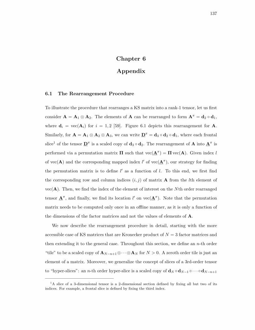
137

Chapter 6

Appendix

6.1 The Rearrangement Procedure

To illustrate the procedure that rearranges a KS matrix into a rank-1 tensor, let us first

consider A = A1 ⊗A2. The elements of A can be rearranged to form Aπ = d2 d1,

where di = vec(Ai) for i = 1, 2 [59]. Figure 6.1 depicts this rearrangement for A.

Similarly, for A = A1 ⊗A2 ⊗A3, we can write Dπ = d3 d2 d1, where each frontal

slice1 of the tensor Dπ is a scaled copy of d3 d2. The rearrangement of A into Aπ is

performed via a permutation matrix Π such that vec(Aπ) = Π vec(A). Given index l

of vec(A) and the corresponding mapped index l′ of vec(Aπ), our strategy for finding

the permutation matrix is to define l′ as a function of l. To this end, we first find

the corresponding row and column indices (i, j) of matrix A from the lth element of

vec(A). Then, we find the index of the element of interest on the Nth order rearranged

tensor Aπ, and finally, we find its location l′ on vec(Aπ). Note that the permutation

matrix needs to be computed only once in an offline manner, as it is only a function of

the dimensions of the factor matrices and not the values of elements of A.

We now describe the rearrangement procedure in detail, starting with the more

accessible case of KS matrices that are Kronecker product of N = 3 factor matrices and

then extending it to the general case. Throughout this section, we define an n-th order

“tile” to be a scaled copy of AN−n+1⊗· · ·⊗AN for N > 0. A zeroth order tile is just an

element of a matrix. Moreover, we generalize the concept of slices of a 3rd-order tensor

to “hyper-slices”: an n-th order hyper-slice is a scaled copy of dN dN−1 · · · dN−n+1

1A slice of a 3-dimensional tensor is a 2-dimensional section defined by fixing all but two of itsindices. For example, a frontal slice is defined by fixing the third index.

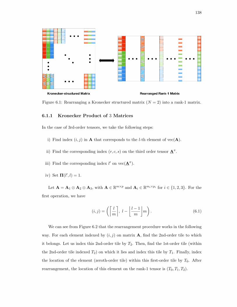
138

Figure 6.1: Rearranging a Kronecker structured matrix (N = 2) into a rank-1 matrix.

6.1.1 Kronecker Product of 3 Matrices

In the case of 3rd-order tensors, we take the following steps:

i) Find index (i, j) in A that corresponds to the l-th element of vec(A).

ii) Find the corresponding index (r, c, s) on the third order tensor Aπ.

iii) Find the corresponding index l′ on vec(Aπ).

iv) Set Π(l′, l) = 1.

Let A = A1 ⊗A2 ⊗A3, with A ∈ Rm×p and Ai ∈ Rmi×pi for i ∈ 1, 2, 3. For the

first operation, we have

(i, j) =

(⌈l

m

⌉, l −

⌊l − 1

m

⌋m

). (6.1)

We can see from Figure 6.2 that the rearrangement procedure works in the following

way. For each element indexed by (i, j) on matrix A, find the 2nd-order tile to which

it belongs. Let us index this 2nd-order tile by T2. Then, find the 1st-order tile (within

the 2nd-order tile indexed T2) on which it lies and index this tile by T1. Finally, index

the location of the element (zeroth-order tile) within this first-order tile by T0. After

rearrangement, the location of this element on the rank-1 tensor is (T0, T1, T2).

139

In order to find (T0, T1, T2) that corresponds to (i, j), we first find T2, then T1, and

then T0. To find T2, we need to find the index of the 2nd-order tile on which the element

indexed by (i, j) lies:

T2 =

⌊j − 1

p2p3

⌋︸︷︷︸

S2j

m1 +

⌊i− 1

m2m3

⌋︸︷︷︸

S2i

+1, (6.2)

where S2j and S2

i are the number of the 2nd-order tiles on the left and above the tile

to which the element belongs, respectively. Now, we find the position of the element in

this 2nd-order tile:

i2 = i− S2im2m3 = i−

⌊i− 1

m2m3

⌋m2m3,

j2 = j − S2j p2p3 = j −

⌊j − 1

p2p3

⌋p2p3. (6.3)

For the column index, T1, we have

T1 =

⌊j2 − 1

p3

⌋︸︷︷︸

S1j

m2 +

⌊i2 − 1

m3

⌋︸︷︷︸

S1i

+1. (6.4)

The location of the element on the 1st-order tile is

i1 = i2 − S1im3 = i2 −

⌊i2 − 1

m3

⌋m3,

j1 = j2 − S1j p3 = j2 −

⌊j2 − 1

p3

⌋p3. (6.5)

Therefore, T0 can be expressed as

T0 = (j1 − 1)m3 + i1. (6.6)

Finally, in the last step we find the corresponding index on vec(Aπ) using the

140

following rule.

l′ =(T2 − 1)m2m3p2p3 + (T1 − 1)m3p3 + T0. (6.7)

6.1.2 The General Case

We now extend our results to N -th order tensors. Vectorization and its adjoint opera-

tion are easy to compute for tensors of any order. We focus on rearranging elements of

A = A1 ⊗A2 ⊗ · · · ⊗AN to form the N -way rank-1 tensor Aπ, where An ∈ Rmn×pn

for n ∈ [N ], A ∈ Rm×p, and Aπ ∈ RmNpN×mN−1pN−1×···×m1p1 .

We first formally state the rearrangement and then we explain it. Similar to the

case of N = 3 explained earlier, for each element of the KS matrix A indexed by (i, j),

we first find the (N − 1)th-order tile to which it belongs, then the (N − 2)th-order tile,

and so on. Let TN−1, TN−2, · · · , T0 denote the indices of these tiles, respectively. Then,

after rearrangement, the element indexed (i, j) on KS matrix A becomes the element

indexed T0, · · · , TN−1 on the rearrangement tensor Aπ.

Now, let us find the indices of the tiles of KS matrix A to which the element (i, j)

belongs. In the following, we denote by (in, jn) the index of this element within its

nth-order tile. Note that since A is an Nth-order tile itself, we can use (iN , jN ) instead

of (i, j) to refer to the index of the element on A for consistency of notation. For the

(iN , jN )-th element of A we have

TN−1 =

⌊jN − 1

ΠNt=2 pt

⌋︸︷︷︸

SNj

m1 +

⌊iN − 1

ΠNt=2 mt

⌋︸︷︷︸

SNi

+1,

iN−1 = iN − SNi ΠNt=2 mt.

jN−1 = jN − SNj ΠNt=2 pt,

where TN−1 is the index of the (N − 1)-th order tile and (iN−1, jN−1) is the location of

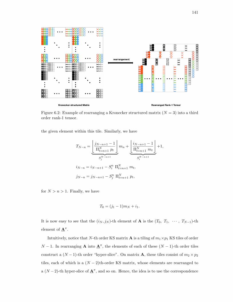
141

Figure 6.2: Example of rearranging a Kronecker structured matrix (N = 3) into a thirdorder rank-1 tensor.

the given element within this tile. Similarly, we have

TN−n =

⌊jN−n+1 − 1

ΠNt=n+1 pt

⌋︸︷︷︸

SN−n+1j

mn +

⌊iN−n+1 − 1

ΠNt=n+1 mt

⌋︸︷︷︸

SN−n+1i

+1,

iN−n = iN−n+1 − Sni ΠNt=n+1 mt,

jN−n = jN−n+1 − Snj ΠNt=n+1 pt,

for N > n > 1. Finally, we have

T0 = (j1 − 1)mN + i1.

It is now easy to see that the (iN , jN )-th element of A is the (T0, T1, · · · , TN−1)-th

element of Aπ.

Intuitively, notice that N -th order KS matrix A is a tiling of m1×p1 KS tiles of order

N − 1. In rearranging A into Aπ, the elements of each of these (N − 1)-th order tiles

construct a (N − 1)-th order “hyper-slice”. On matrix A, these tiles consist of m2× p2

tiles, each of which is a (N − 2)th-order KS matrix, whose elements are rearranged to

a (N − 2)-th hyper-slice of Aπ, and so on. Hence, the idea is to use the correspondence

142

between the nth-order tiles and nth-order hyper-slices: finding the index of the n-th

order tile of A on which (i, j) lies is equivalent to finding the index of the nth-order

hyper-slice of Aπ to which it is translated. Note that each entry of a tensor in indexed

by an N -tuple and the index of an entry of a tensor on its nth hyper-slice is in fact its

nth element in the index tuple of this entry. Therefore, we first find the (N−1)-th order

KS tile of A on which the (i, j) element lies (equivalent to finding the (N − 1)th-order

hyper-slice to which (i, j) is translated), and then find the location (iN−1, jN−1) of this

element on this tile. Next, the (N − 2)-th order KS tile in which (iN−1, jN−1) lies is

found as well as the location (iN−2, jN−2) of the element within this tile, and so on.

6.2 Properties of the Polynomial Sequence

Here, we analyze the polynomial sequence (5.18) in the following lemma (Lemma 22)

and its corollary (corollary 4).

Lemma 22. Given the polynomial sequence pt(x) defined as

pt(x) = (1 + ηx)pt−1(x)− βpt−2(x), p1(x) = 1 + ηx, p0(x) = 1, (6.8)

if y 6= 4β, we have

pt(x) =1√

y2 − 4β

(y +√y2 − 4β

2

)t+1

−

(y −

√y2 − 4β

2

)t+1 (6.9)

and if y = 4β,

pt(x) = (t+ 1)(√β)t (6.10)

where y = 1 + ηx.

Proof of Lemma 22. Consider the generation function of the sequence pt(x), i.e.,

143

G(x, z) =∑∞

t=0 pt(x)zt, z ∈ C. It follows from update rule (6.8) that

∞∑t=1

pt+1(x)zt+1 =∞∑t=1

(1 + ηx)pt(x)zt+1 − β∞∑t=1

pt−1(x)zt+1

G(x, z)− p0 − p1z = (1 + ηx)z(G(x, z)− p0)− βz2G(x, z)

G(x, z)(1− (1 + ηx)z + βz2) = p0 + (p1 − (1 + ηx)p0)z (6.11)

Therefore, plugging in the values of p0 and p1 results in

G(x, z) =p0 + (p1 − (1 + ηx)p0)z

1− (1 + ηx)z + βz2=

1

1− (1 + ηx)z + βz2(6.12)

Let y , 1 + ηx. Then,

G(y, z) =1

1− yz + βz2=

1

β(z − r1)(z − r2)(6.13)

where r1 and r2 are the roots of βz2 − yz + 1, i.e. we have r1,2 =y±√y2−4β

2β . When

144

r1 6= r2 we have

G(y, z) =1

β(z − r1)(z − r2)

=1

β(r1 − r2)

(1

r2 − z− 1

r1 − z

)=

1

β(r1 − r2)

(1

r2(1− z/r2)− 1

r1(1− z/r1)

)Taylor Expansion

=1

β(r1 − r2)

∞∑t=0

(zt

rt+12

− zt

rt+11

)

=1

βy(r1 − r2)

∞∑t=0

(zt

rt+12

− zt

rt+11

)

=1

β(r1 − r2)

∞∑t=0

(zt

rt+12

− zt

rt+11

)

=1

β(r1 − r2)

∞∑t=0

(zt

rt+12

− zt

rt+11

)

=∞∑t=0

[1/r2

β(r1 − r2)

(1

r2

)t− 1/r1

β(r1 − r2)

(1

r1

)t]zt

=∞∑t=0

[r1

r1 − r2

(1

r2

)t− r2

r1 − r2

(1

r1

)t]zt (6.14)

Since r1,2 =y±√y2−4β

2β , we have r1 − r2 =

√y2−4ββ and r1r2 = 4β

4β2 = 1β . Therefore,

when |z| < |r2|, G(x, z) is well defined, we have

pt(x) =r1

r1 − r2

(1

r2

)t− r2

r1 − r2

(1

r1

)t=

r1

r1 − r2(r1β)t − r2

r1 − r2(r2β)t

=r1

r1 − r2

(y +

√y2 − 4β

2

)t− r2

r1 − r2

(y −

√y2 − 4β

2

)t

=y +

√y2 − 4β

2√y2 − 4β

(y +

√y2 − 4β

2

)t− y −

√y2 − 4β

2√y2 − 4β

(y −

√y2 − 4β

2

)t

=1√

y2 − 4β

(y +√y2 − 4β

2

)t+1

−

(y −

√y2 − 4β

2

)t+1

On the other hand, when x =, we have y = 2√β and r1 = r2 = 1√

β. Thus,

G(y, z) =1

β(z − r1)(z − r2)

=1

(√βz − 1)2

Taylor expansion=

∞∑t=0

(t+ 1)(√βz)t (6.15)

When z < 1/√β, G(x, z) is well-defined. Therefore, pt(

2√β−1η ) = (t+ 1)(

√β)t.

Corollary 4. Consider polynomial sequence pt(x) defined as in (6.8). Then we have

K∏k=1

ptk(x) ≤ 1

(√y2 − 4β)K−1

pK−1+∑Kk=1 tk

(x) (6.16)

Proof of Corrolary 4. We know from (6.9) that

pt(x) =1

β(r1 − r2)(rt+1

1 − rt+12 )

=1√

y2 − 4β

(y +√y2 − 4β

2

)t+1

−

(y −

√y2 − 4β

2

)t+1

It follows that

pi(x)pj(x) =1

β2(r1 − r2)2(ri+1

1 − ri+12 )(rj+1

1 − rj+12 )

=1

β2(r1 − r2)2(ri+1

1 rj+11 + ri+1

2 rj+12 − ri+1

2 rj+11 − ri+1

1 rj+12 )

(a)

≤ 1

β2(r1 − r2)2(ri+1

1 rj+11 + ri+1

2 rj+12 − ri+1

2 rj+12 − ri+1

2 rj+12 )

=1

β2(r1 − r2)2(ri+j+2

1 − ri+j22 )

=1

β(r1 − r2)pi+j+1(x)

=1√

y2 − 4βpi+j+1(x) (6.17)

Therefore, we can easily use induction to prove the corollary.

Documents

NONCONVEX MATRIX AND TENSOR RECOVERY WITH …