Soil & Tillage Research 191 (2019) 306-316

ELSEVIER

Contents lists available at ScienceDirect

Soil & Tillage Research

journal homepage: www.elsevier.com/locate/still

Photogrammetric analysis tools for channel widening quantification under laboratory conditionsChao Qina,b,c, Robert R. Wellsc, Henrique G. Mommd, Ximeng Xua,c, Glenn V. Wilsonc,Fenli Zhenga,e’*a State Key Laboratory of Soil Erosion and Dryland Farming on the Loess Plateau, Northwest A&F University, Yangling 712100, Shaanxi, Chinab State Key Laboratory of Hydroscience and Engineering, Tsinghua University, Beijing 100084, Chinac USDA-ARS National Sedimentation Laboratory, Oxford 38655, MS, USAd Department of Geosciences, Middle Tennessee State University, Murfreesboro, TN 37130, USAe Institute of Soil and Water Conservation, CAS & MWR, Yangling 712100, Shaanxi, China

Check for updates

ABSTRACTARTICLE INFO

Keywords:Soil erosionGully Photogrammetry Concentrated flowSediment discharge

Accurate soil erosion monitoring provides a basis for soil erosion prediction and prevention. Channel bank erosion quantification is prerequisite to couple effectively the bank sediment supply system with fluvial sediment transport fluxes. The objectives of this study were to describe and evaluate methods for monitoring and data post-analysis of channel widening in the presence of a non-erodible layer. Technology was developed to capture 5-cm spaced cross-sections along a soil flume at 3-s time intervals. Two off-the-shelf digital cameras were po­sitioned 3-m above the soil bed and controlled by a program to trigger simultaneously and download images to the computer. Methods utilizing color differences in images and elevation differences in DEMs were applied to detect discontinuities between channel walls and the soil bed. Channel widths were calculated by differentiating the coordinates of these surface discontinuities. A volumetric method was used to calculate flow velocity with measurements of flow depths obtained from ultrasonic depth sensors. Sediment concentration was determined by manual sampling. The results showed that different channel width calculation methods exhibited comparable outcomes and achieved satisfactory accuracy. Sediment discharge showed a significant positive linear correla­tion with channel widening rate, while exhibiting a 5 to 25-s time lag compared to the peak of channel widening rate. Total sediment discharge calculated by photogrammetry was 3.1% lower than that calculated by manual sampling. Flow velocity decreased with time and showed a significant negative power correlation with channel width. Advantages of the described methodology include automated high spatial and temporal monitoring re­solution, semi-automated data post-processing, and the potential to be generalized to large scale river/reservoir bank failure monitoring.

1. Introduction

Soil erosion is a serious problem in agricultural regions that threa­tens food security in many countries. The impact of soil erosion on modem society demands accurate descriptions on when, where and how soil erosion occurs and on process descriptions which can provide fundamental knowledge for prediction (Guo et al., 2016; Prosdocimi et al., 2017). However, data collection efforts are often inadequate to quantify various soil erosion processes and their inherent interactions, though many technologies have been developed by soil and geomor­phology scientists to acquire detailed information on the variation in the soil surface caused by erosion (Lawler et al., 1997; Nouwakpo and

Huang, 2012; Gomez-Gutierrez et al., 2014; Wells et al., 2016; Prosdocimi et al., 2017).

Soil erosion by water is widely accepted to be classified into sheet, rill, and gully (classical and ephemeral) or channel erosion (Foster and Meyer, 1972). However, many of the widely-used soil erosion predic­tion models such as USLE and WEPP have not addressed the mechan­isms of gully erosion, which might lead to an underestimation of soil loss in agricultural fields (Bennett et al., 2000b; Thomas et al., 1986). Gully erosion, which has been recognized in recent years, is a major contributor to sediment yield in watersheds (Poesen et al., 2003; Castillo and G6mez, 2016). Once formed, gully channels develop quickly with three main physical processes: headcut migration, bed

• Corresponding author at: No. 26, Xi’nong Road, Institute of Soil and Water Conservation, Yangling 712100, Shaanxi, China.E-mail addresses: glqinchao@nwsuaf.edu.cn (C. Qin), Robert.Wells@ars.usda.gov (R.R. Wells), Henrique.Momm@mtsu.edu (H.G. Momm),

xuxm@igsnrr.ac.cn (X. Xu), Wilson@ars.usda.gov (G.V. Wilson), flzh@ms.iswc.ac.cn (F. Zheng).

https://doi.org/10.1016/j-still.2019.04.002Received 30 June 2018; Received in revised form 8 March 2019; Accepted 4 April 20190167-1987/ © 2019 Elsevier B.V. All rights reserved.

C. Qin, etaL Soil & Tillage Research 191 (2019) 306-316

incision and bank expansion (widening) (Bennett et al., 2000a; Alonso et al., 2002; Wells et al., 2013; Bingner et al., 2016). Chaplot et al. (2011) reported that bank failure was confirmed to be a main process after headcut migration in overall gully evolution and overall erosion in landscapes.

Concentrated flow erosion generally occurs in two phases: down­ward incision and subsequent channel widening (Bennett et al., 2000b; Casalf et al., 2003; Wells et al., 2013; Qin et al., 2018a, b). Much re­search has been conducted on widening of large channel systems such as rivers and streams but considerably less on gullies. The basic pro­cesses are the same which include fluvial erosion of the bank toe, see­page erosion, and mass failure, generally in response to undercutting by fluvial and/or seepage erosion (Lawler et al., 1997; Rinaldi and Darby, 2007; Fox and Wilson, 2010; Masoodi et al., 2018). Due to a continuum representation and replacement to all the rapidly fluctuating spatial heterogeneity from small rills to large river channels, fluvial erosion, i.e. erosion of the sidewall toe (undercutting) by surface flow, could be used to describe channel sidewall expansion processes (Govindaraju and Kawas, 1992). Lawler et al. (1997) reviewed methods of mon­itoring riverbank erosion and discussed the importance of having a monitoring system that captures the timing and magnitude of erosion events with the driving forces or mechanisms. They noted that without such monitoring capabilities, it is “difficult to couple effectively the bank sediment supply system with fluvial sediment transport fluxes ... hinders the identification of the processes and mechanisms of river bank erosion.”

Gully erosion is strongly influenced by anthropogenic factors such as tillage operations (Foster, 1986). Non/less-erodible layers, which have a resistance to erosion greater than that of the overlying soil, often develop due to conventional tillage operations and heterogeneities between bed rock/plow pan and tilled layers (Piest et al., 1975; Foster, 2005; Gordon et al., 2007; Wells et al., 2013). This more erosion-re­sistant layer limits channel incision forcing the channel to expand lat­erally through basal scour of the bank toe and gravitational mass movement of the channel sidewalls (Bingner et al., 2016). Gully widening accelerates at the interface between the plow layer and the less-erodible layer, as the energy of the flowing water shifts from a vertical force to a horizontal force. Research on channel width variation alone or in combination with other processes and applicable meth­odologies have been developed in both field and laboratory settings (Chaplot et al., 2011; Chen et al., 2013; Wells et al., 2013; Momm et al., 2015; Wells et al., 2016; Masoodi et al., 2018; Yang et al., 2017). The edge detection methods to depict channel width changes developed by Momm et al. (2015) provided a foundation for the current research. Based on measuring the electromagnetic energy, an indirect measure­ment of topographic discontinuities has been introduced to monitor temporal and spatial variations of channel width. These authors used one single camera to capture images under a strictly controlled lighting condition, then they developed computer programs, integrated with open source computer libraries, to automatically measure and calculate channel width with satisfactory results.

Concentrated flow erosion, in most cases, is responsible for gully formation and evolution on cropland (Foster, 1986; Thomas et al., 1986; Romkens et al., 2001). Overland concentrated flow character­istics, including flow depth, width and velocity are hard to be accu­rately monitored due to their shallow flow depth, high flow velocity, sediment concentration and rapidly changing channel morphology (Lei et al., 2005; Dong et al., 2014). Traditional measuring methods such as the water level gauge pins and the dye tracing method are strongly influenced by subjective readings of both the gauge pin, stop watch and initial and final lines of dye material estimation. The velocities mea­sured by the dye tracing method need to be re-calibrated or corrected with different correction factors to get the average velocity, with no universally acceptable and applicable correction coefficients (Dong et al., 2014). The volumetric method, based on the calculation of the product of flow depth, width and velocity, has been used in recent

studies (Gimenez et al., 2004; Dong et al., 2014). However, under a certain inflow rate, flow depth is hard to detect while flow width is easier to define through measurement on a photo or video. As a result, ultrasonic water depth sensors were introduced into this research as they have been widely used in river water depth observation.

Rill/gully erosion, relatively easier to be detected compared to sheet erosion, has been widely monitored by total station and high precision GPS (RTK) survey, laser scanning (LiDAR), and photogrammetry (Casalf et al., 2006; Eitel et al., 2011; Castillo et al., 2012; Frankl et al., 2015; Vinci et al., 2015; Guo et al., 2016; Wells et al., 2016; Qin et al., 2018c). Researches based on the above methodologies has greatly deepened the understanding of the magnitude of rill/gully erosion. Photogrammetry is a simple, robust means to track landscape evolution and morpho- dynamic changes in rills and gullies. Cameras are easier to operate compared with the 3D laser scanner, and a digital photogrammetric system allows operators to scale according to their own requirements (Castillo et al., 2012; Frankl et al., 2015; Guo et al., 2016; Wells et al., 2016). Photogrammetry has advantages of being cost-effective, labor saving, reliable, and the analysis and presentation can be automated (Wells et al., 2016). However, current photogrammetry methodology still needs to be improved, e.g. automated system for detecting channel erosion and image post-processing based on GIS platform. Moreover, it is necessary to compare different methods regarding image post-pro- cessing in order to select optimal and simple methods for photo­grammetry popularization.

Since concentrated flow experiments are suitable for simulating channel evolution processes (Zhu et al., 1995; Wells et al., 2013; Qin et al., 2018b), in this study, a concentrated flow experiment, combined with photogrammetry, was employed to investigate channel widening when the channel was constrained vertically by the presence of a non- erodible layer. The objectives of this study were to: 1) quantify channel widening by fluvial and mass failure processes using photogrammetry; 2) compare three methodologies regarding image post-processing; 3) quantify the response of sediment discharge and flow velocity to channel widening.

2. Materials and methods

2.1. Data collection systems

2.1.1. Photogrammetry systemThe photogrammetry system consists of a laptop, two cameras,

connecting wires and a matched coded computer program (Figs. 1 and 2). Linux operating system was used to write the specific program to control and simultaneously shoot photos with the two cameras. Two Nikon D7000 cameras (Nikon Inc., Melville, NY, USA) were used to capture paired images. Two USB wires connected the cameras with the laptop so that the paired images could be transferred and stored in the laptop. The intervals between two shootings could be set as fast as two seconds.

2.1.2. Channel widening simulation systemA soil box measuring 3.89 m-long, 0.61 m-wide and 0.30 m-deep,

containing a drainage pipe system at the soil box bottom, was used in this study. The soil box may be inclined in 0.1% adjustment steps to achieve slope gradients between 0 and 12% (Fig. 2). A runoff outlet at the downstream end of the soil box was used to collect runoff samples throughout the experiment.

The soil used in this study was Atwood sandy clay loam (fine-silty and mixed), which can be classified as a Typic Paleudalfs (NRCS USDA, 1999). The soil was collected at a well-drained site in Pontotoc, Mis­sissippi, USA. Impurities, such as large organic matter and gravel, were removed from the soil. Then, soil was dried, crushed and passed through a 4-mm sieve prior to packing. The average mass soil water content before packing was 2.5 ± 0.5% for all treatments.

307

C. Qin, etaL Soil & Tillage Research 191 (2019) 306-316

Rainfall/ Inflow rate

Initial outputHardwarei

parameters

ii

ii i

i i i

Rainfall simulator, water tank-pump

system, laptop

Ultrasonic wave generators, laptop,

connections

! Systemiiii

i J Software

Variation of channel width & sediment concentration

i i

1 1

Logger Net

)H Nozzle pressure, flow rate.

60 s interval

• i* 11 1

[ 1

Labview Voltage.0.1 s interval

Data interpretation

Average nozzle pressure H Rainfall intensity'

Flow rate per min

Channel width—► Flow width

Flow depth Flow rate

------------\ Flow

velocity

------------------------ 1 11 1

Channel \ ;width / i i

i i

Cameras, laptop, connections

■0

J 1

Linux '& VBA J

Paired photos.3 s interval

■ i 1 11 1 •!• i

1 1Sediment '

concentration J\ i1 1

Pre-made channel, bottles, scales,

oven

ii: i

Manually ' measuring J

RunoffZsediment weight.

20 s interval

Edse detection from left/right sides| Single photo |hl Spatial adjustment +R.G.B 1

light channel wave length ||->|

| Paired photos |hl 3D point clouds, raw/ 1georeferenced orthophotos | ►1

| Paired photos |H 3D point clouds (txt 1format). Tin +fishnet. DEM |hL

Wave discontinuity' and edge detection

Elevation discontinuity and edge detection

Channel width in3 ways

■xRelationship between channel width and sediment

concentration/concentrated flow velocity'

Channel widening simulation and data interpretation

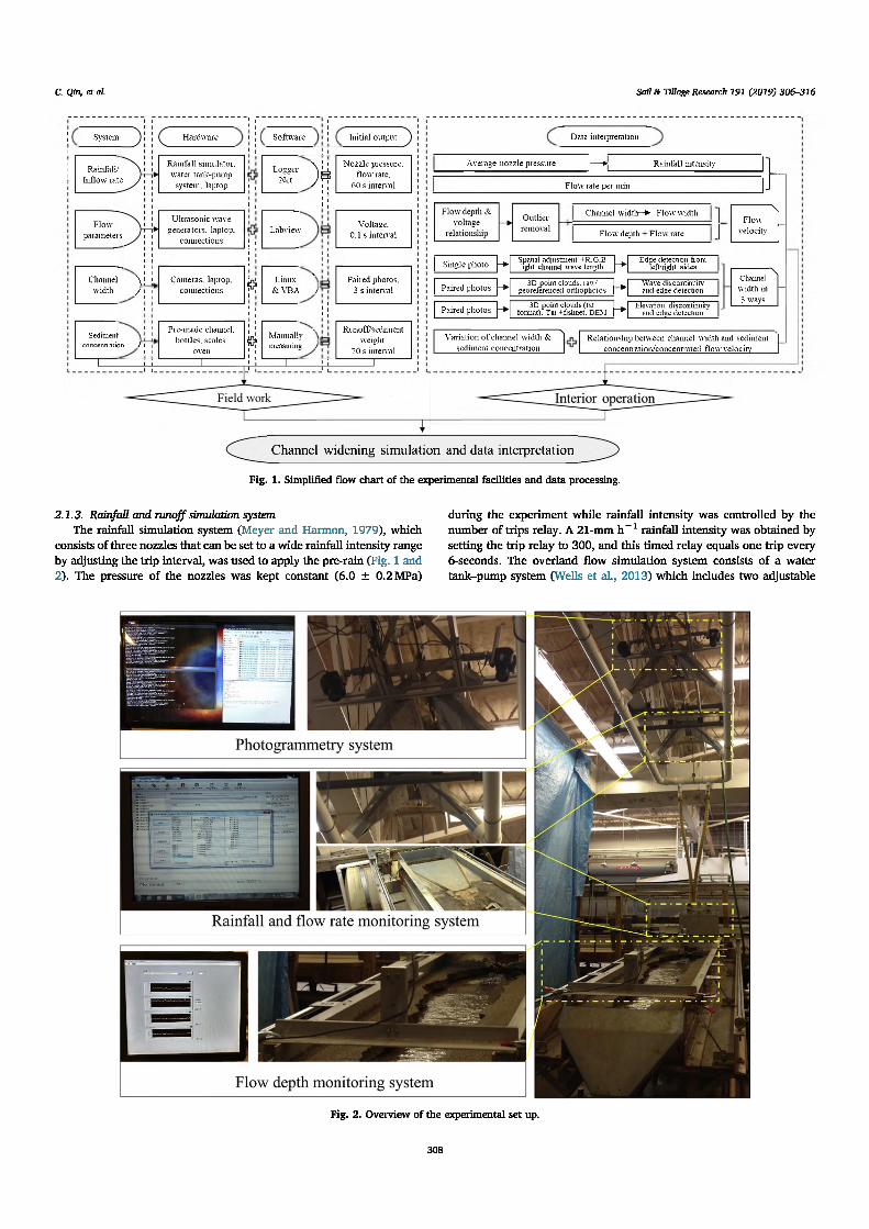
Fig. 1. Simplified flow chart of the experimental facilities and data processing.

2.1.3. Rainfall and runoff simulation systemThe rainfall simulation system (Meyer and Harmon, 1979), which

consists of three nozzles that can be set to a wide rainfall intensity range by adjusting the trip interval, was used to apply the pre-rain (Fig. 1 and 2). The pressure of the nozzles was kept constant (6.0 ± 0.2 MPa)

during the experiment while rainfall intensity was controlled by the number of trips relay. A 21-mm h_1 rainfall intensity was obtained by setting the trip relay to 300, and this timed relay equals one trip every 6-seconds. The overland flow simulation system consists of a water tank-pump system (Wells et al., 2013) which includes two adjustable

Fig. 2. Overview of the experimental set up.

308

C. Qin, etaL Soil & Tillage Research 191 (2019) 306-316

intake valves.The rainfall/overland flow monitoring system includes a paddle

wheel flow meter, a laptop and matched software (LoggerNet 4.2.1, Campbell Scientific Incorporation). The real-time pressure of the noz­zles and inflow rate can be read from the screen and recorded in one- minute intervals. After setting the time, the above data can be exported in tabular format for further analysis (Figs. 1 and 2).

2.1.4. Concentrated flow depth measuring systemThe ultrasonic depth measurement system consists of a desktop

computer, two ultrasonic depth sensors and matched software (Figs. 1 and 2). The ultrasonic depth sensors (TS-30S1-IV, Senix Co., TV, USA) were connected with the desktop computer through a junction box and controlled by Labview 7.1 (National Instruments Corp., Austin, TX, USA). The stored information was text format and included the fol­lowing: time, flow voltage, upstream voltage, and downstream voltage. The ultrasonic sensor frequency can be set to as fast as one millisecond.

2.2. Datn collection processes

2.2.1. Channel model establishmentThe procedure to establish the channel model was similar to Wells

et al. (2013). Detailed steps are described as follows:

1) Filling soil box: soil was packed above a 0.03-m subsurface drainage system (tile line) that was covered by fine sand, and a highly permeable cloth was used to separate the drainage layer and soil layers. Soil was then packed above the drainage system to a total depth of 0.16-m in 0.03-m increments (75-kg) by vibration trans­mitted through a plywood plate.

2) Establishment of non-erodible layer: a 0.01-m non-erodible layer, whose strength was large enough to resist the concentrated flow, was placed at the center of the soil box (5 to 1 mixture of soil and thin-set mortar). This layer was established to simulate the plow pan developed due to conventional tillage operations, which may have significant impacts on channel bed incision and sidewall expansion (Wells et al., 2013; Bingner et al., 2016; Qin et al., 2018a,b). The non-erodible layer was subjected to a 21-mm h_ 1 pre-rain lasting 1- h and then packed for 0.2-h by vibration (Gordon et al., 2007). To cure the non-erodible layer, a fan forced air over the surface for 24- h.

3) Establishment of channel model: once the non-erodible bed was dried out and hardened, an orthogonal aluminum channel (2.5-m long, 0.04-m wide, 0.04-m deep) was placed in the center of the soil bed and soil was packed around the channel in 75-kg increments by vibration. The channel was leveled with the downstream outlet of the low-drop structure and a small curvature (2-m radius; 0.02-m elevation increase from channel top bank to soil flume edge) was cut into the soil bed at the upper entrance into the channel (Fig. 1). After overnight self-settling (12-h), a second pre-rain of 21-mm h_1 was applied for 3-h to the soil bed with a 5% slope gradient. This ensured that no water ponded on the soil surface. The purpose of the second pre-rain was to develop consistent soil moisture, consolidate loose soil particles by raindrop impact, and reduce the spatial variability of underlying soil conditions. After the second pre-rain, the orthogonal aluminum channel was slowly pulled out of the soil bed starting at the downstream end of the soil box. The transition section connecting the inflow baffle and soil material at the upper curvature entrance into the channel was protected with rubberized paint (Rust-Oleum truck bed coating1). A summary of experimental parameters is given in Table 1.

’Manufactured by Rust-Oleum Corporation, 11 Hawthorn Pkwy., Vernon Hills, IL, USA, 60061

Table 1Summary of experimental parameters.

Factors Value

Upslope inflow rate/L s-1 1.08Slope gradient/% 5Initial channel width/cm 10Initial channel depth/cm 4Soil bulk density/kg m-3 1390Infiltration rate/L s-1 0.00417Experimental duration/s 420

2.2.2. Layout of control pointsSimilar to Wells et al. (2013), 10 permanent photogrammetry tar­

gets with unique ID (RAD coded), parallel to the soil surface, were setup at the boundary of the soil box (Figs. 3 and 4a). To obtain the exact x, y, z coordinates of each target, the relative position (the distance) of each target was measured manually with a 1-mm precision steel ruler. The coordinates were set for the left bottom most target as 100, 100, 100, the relative coordinates of the other targets were calculated by their distances (Fig. 3). The difference between measured distance and checked distance ranged between -0.16 to 0.06-mm and relative errors were -0.10%-0.11%, which showed satisfactory accuracy (Table 2). Compared to the measuring method by total station, the manual mea­surements have the advantages of easily operating, low cost and time/ workforce effective.

2.2.3. Paired images obtainingPhotogrammetiy was used to capture the characteristics of channel

widening and micro-distortion of the soil surface. At slope length of 150-cm, two cameras (Nikon D7000) were mounted 3-m above the soil bed (Figs. 1 and 2) and were calibrated according to the standard camera calibration procedure using PhotoModeler Scanner 2017.0.1 version (Eos Systems Inc., Vancouver, Canada) to ensure that the cameras were tuned to the specific experimental environment (light and reflection). Light was controlled and kept constant during the experi­ment. Cameras were set to an appropriate position to ensure that the photos were parallel to the soil surface and had an overlap of 95%. Then, adjustments were made to both cameras: 1) Set shooting type to RAW with the highest camera resolution (4928 x 3264 pixel, 300 x 300 dpi); 2) Selected auto scene mode (AF) and focused auto­matically until clear photos were obtained, then set focus mode to manual focus (MF). The detailed final parameters were as follows: f/2.8 aperture, 800 ISO, 1/60 s exposure time, 20 mm focal length; 3) Image storage path was determined by USB port detection; 4) Image collection frequency was set to three seconds; 5) Chose a specified store path and sent shell commands to trigger the cameras simultaneously; 6) Paired images were then imported into PhotoModeler Scanner after the phy­sical experiment for processing (Fig. 4 a, b).

2.2.4. Runoff, sediment dam and final channel width measurementExperiments were conducted by applying inflow to the channel at a

rate of 1.08-L s_1. Runoff and sediment samples were captured in 0.5-L glass bottles at 20-s intervals. The infiltrated water was collected by a separate bucket at the outlet of the underlined drainage pipe during 420-s experimental time. Sediment samples were weighed, settled (24-h storage), and dried in an oven at 105 °C for 24-h after decanting, then reweighed (Fig. 1). Water surface (WS) elevations of concentrated flow were measured on 10-milisecond intervals by ultrasonic distance sen­sors mounted above the flume at upstream and downstream positions (Wells et al., 2013) (Figs. 1 and 2). The distance between the two sensors was 150.5-cm. Soil bulk density was determined by extracting undisturbed cores using aluminum rings with a 61.8-mm diameter and a 20.0-mm height at middle slope position on both left and right channel banks after the experiment.

A re-defined coordinate system was established for manual

309

C. Qin, etaL Soil & Tillage Research 191 (2019) 306-316

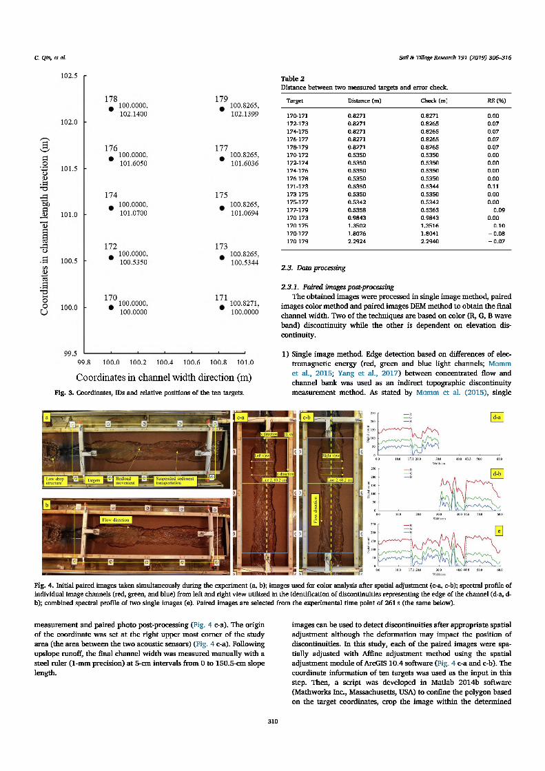
Coordinates in channel width direction (m)Fig. 3. Coordinates, IDs and relative positions of the ten targets.

Table 2Distance between two measured targets and error check.

Target Distance (m) Check (m) RE (%)

170-171 0.8271 0.8271 0.00172-173 0.8271 0.8265 0.07174-175 0.8271 0.8265 0.07176-177 0.8271 0.8265 0.07178-179 0.8271 0.8265 0.07170-172 0.5350 0.5350 0.00172-174 0.5350 0.5350 0.00174-176 0.5350 0.5350 0.00176-178 0.5350 0.5350 0.00171-173 0.5350 0.5344 0.11173-175 0.5350 0.5350 0.00175-177 0.5342 0.5342 0.00177-179 0.5358 0.5363 -0.09170-173 0.9843 0.9843 0.00170-175 1.3502 1.3516 -0.10170-177 1.8026 1.8041 -0.08170-179 2.2924 2.2940 -0.07

2.3. Data processing

2.3.1. Paired images postprocessingThe obtained images were processed in single image method, paired

images color method and paired images DEM method to obtain the final channel width. Two of the techniques are based on color (R, G, B wave band) discontinuity while the other is dependent on elevation dis­continuity.

1) Single image method. Edge detection based on differences of elec­tromagnetic energy (red, green and blue light channels; Momm et al., 2015; Yang et al., 2017) between concentrated flow and channel bank was used as an indirect topographic discontinuity measurement method. As stated by Momm et al. (2015), single

Fig. 4. Initial paired images taken simultaneously during the experiment (a, b); images used for color analysis after spatial adjustment (c-a, c-b); spectral profile of individual image channels (red, green, and blue) from left and right view utilized in the identification of discontinuities representing the edge of the channel (d-a, d- b); combined spectral profile of two single images (e). Paired images are selected from the experimental time point of 261 s (the same below).

measurement and paired photo post-processing (Fig. 4 c-a). The origin of the coordinate was set at the right upper most comer of the study area (the area between the two acoustic sensors) (Fig. 4 c-a). Following upslope runoff, the final channel width was measured manually with a steel ruler (1-mm precision) at 5-cm intervals from 0 to 150.5-cm slope length.

images can be used to detect discontinuities after appropriate spatial adjustment although the deformation may impact the position of discontinuities. In this study, each of the paired images were spa­tially adjusted with Affine adjustment method using the spatial adjustment module of ArcGIS 10.4 software (Fig. 4 c-a and c-b). The coordinate information of ten targets was used as the input in this step. Then, a script was developed in Matlab 2014b software (Mathworks Inc., Massachusetts, USA) to confine the polygon based on the target coordinates, crop the image within the determined

310

C. Qin, etaL Soil & Tillage Research 191 (2019) 306-316

analysis scope, read the R, G, B values of every single pixel and process edge detection at 5-cm intervals from upslope to downslope. The edge detection processing began at the origin point and moved in both X and Y direction (Fig. 4 c-a). Due to the difference between the two cameras’ positions, edge detection begins from the left boundary to the middle of the soil box when the image was taken from the right view and vice versa (Fig. 4 c-a, c-b, d-a and d-b) (Momm et al., 2015). Then, the integrated electromagnetic energy line was determined by the combination of the two images (Fig.4 e). A formula was developed to detect the discontinuities using single image method and paired images color method. Discontinuities were manually pinpointed based on the following formula and their coordinates were recorded (Fig.4 e). The channel width was calcu­lated by the difference between two coordinates. The indicator /J is defined as the change rate of the count of the electromagnetic en­ergy:

= IBWH4--EW.I x 100%(1)

where w, is the channel width (mm), i = 0, 4, 8,...,596 mm, EWj is the count of the electromagnetic energy at the ith channel width (mm). If the Pi > 20%, then the point at the ith channel width was defined as a discontinuity. If the Pi < 20%, then the first point from the left boundary (or the first point from the right boundary) at the ith channel width was recognized as an integral part of the channel wall or channel bed.

1) Paired images color method. An orthophoto is another measurable image obtained from paired images. Processing of paired images was conducted with PhotoModeler Scanner, which included the following steps: point cloud generation, raw orthophoto generation, target recognition, coordinate import and georeferenced orthophoto generation (Fig. 5). The georeferenced orthophotos were then pro­cessed in Matlab2014b (using the same procedure as the single image method above) and final channel widths at each 5-cm interval of slope length were exported.

2) Paired images DEM method. DEMs have been widely used in ana­lyzing topographic changes (Nouwakpo and Huang, 2012; Frank! et al., 2015; Bingner et al., 2016; Guo et al., 2016; Masoodi et al., 2018). DEMs were generated from 3D point clouds in ArcGIS 10.4 (Fig. 6). Following are the procedures of detecting channel widths from initial paired images: 1) georeferenced 3D point cloud gen­eration in PhotoModeler Scanner (target detection, photo

alignment, coordinate transformation and matching); 2) point cloud export from PhotoModeler in. txt format; 3) point cloud import into ArcGIS 10.4 (ESRI Inc., Redlands, CA, USA); 4) DEM construction (making an x, y event layer; creating a triangulated irregular net­work (Tin) and a fishnet of rectangular cells; recreating Tin; and Tin to raster); 5) edge detection based on elevation difference; 6) channel width measurements and export. Refer to the NorToM ap­proach proposed by Castillo et al. (2014), a formula was developed to detect the discontinuities between channel wall and channel bed. The indicator a is defined as the elevation change rate:

Hwi (2)

where w, is the channel width (mm), i = 0, 4, 8,...,596 mm, HWi is the elevation at the ith channel width (cm). If the a, > 20%, then the first point from the left boundary (or the first point from the right boundary) at the ith channel width was defined as a discontinuity. If the at < 20%, then the point at the ith channel width was recognized as an integral part of the channel wall or channel bed.

After applying the procedure above, channel widths at each time step along the slope length were obtained. Based on the 20 channel widths from 0 to 150.5 cm slope length, average channel widths at each time step were calculated.

2.3.2. Concentrated flow width, depth and velocity calculationBefore measuring the flow depth, the ultrasonic distance sensors in

both upstream and downstream direction were calibrated with metal plates of known thickness. The relationship between voltage and flow depth represented by metal plates thickness, and the corresponding fitted regression formulas were depicted in Fig. 7. Channel flow velocity is influenced by flow discharge, bed slope, channel roughness and shapes of channel cross sections. Moore and Burch (1986) derived an equation to calculate the rill channel flow velocity which can be used in this study:

J re0-75 (3)

where V is the flow velocity (cm s_1), Q is the inflow rate (L s_1), I is the infiltration rate (L s_1), J is the number of channels crossing the contour element b, s is bed slope (m m_1), W is a channel shape factor which equals to C0'5, C is a constant that is dependent on the shape of the channel which equals to R/A05, R is the hydraulic radius (cm), A is the cross-sectional area of flow in the channel (cm2). The n is Manning’s

H

Fig. 5. Initial paired images taken simultaneously during the experiment (a, b); point clouds used to generate orthophotos (c); cropped georeferenced orthophotos (d); spectral profile of image channels (red, green, and blue) under different situations (e). Line 1 represents the situation of enough point clouds with failure block, Line 2 represents the situation of enough point clouds without failure block, Line 3 represents the situation of sparse point clouds (The same below).

0 10 11.1 20 30 40 46.4 $0 60

311

C. Qin, etaL Soil & Tillage Research 191 (2019) 306-316

Fig. 6. Initial paired images taken simultaneously during the experiment (a, b); point clouds (c) and TINs (d) used to generate DEMs; generated DEM (e); cross­sections of elevation difference in upstream, middle stream and downstream position (f).

Fig. 7. Calibration of ultrasonic distance sensors (show the relationship be­tween voltages and flow depths represented by metal plates thickness).

roughness coefficient, whose dimension is T/L*(l/3). In this study, I, J, s and n equal to 4.17 x 10'3 L s_1, 1, 0.05 and 0.05, respectively.

3. Results and discussion

3.1. Comparisons of three methodologies in calculating channel width

Fig. 8a shows that the channel widths calculated using the above three methods at different time periods are similar and only exhibit relative errors between 0.3% and 7.0%. Using manual measurement as

Time/min

a Single imagex Paired images color o Paired images DEM

300 360 420

a baseline, the single image method, paired images color method and paired images DEM method showed relative errors of -1.5%-1.8%, -2.7%-2.3% and -1.5%-2.7%, respectively (Fig. 8b).

The paired images DEM method is applicable for edge detection in a variety of circumstances as long as an elevation difference exists. The point clouds generated from a water surface exhibits low precision and may not reflect the actual elevation (Gomez-Gutierrez et al., 2014; Wells et al., 2017). However, in the current study, the elevation dif­ference was enough to accurately detect the channel wall edge point (Fig. 6 e and f). Three representative profiles were selected to study the applicability of the DEM method of edge detection. Lines 1 and 2 re­present the situation with adequate point coverage to generate a DEM while Line 3 represents the situation with limited points of bed detec­tion (Fig. 6 e). All three profile graphs show turning points between the channel wall and channel bed (Fig. 6 f). Channel width was calculated based on the coordinates of turning points. In certain field situations, such as gullies without perennial drainage or deep gullies affected by shadowing, the color methods may not be applicable, and the DEM method would be the best choice.

Methods based on electromagnetic energy (red, green and blue light channels) discontinuities are applicable under the condition that color differences between the channel wall and bed are significant (Figs. 4 c- a, c-b and 5 d; Momm et al., 2015; Yang et al., 2017). This method is useful in distinguishing the boundary between the water body and soil, e.g. water surface area of the reservoir. For a soil surface with different soil water contents, this method is also applicable by distinguishing color differences of different regions of the soil surface.

25

45

g 40

| 35Q

CS

U 30a Single image x Paired images coloro Paired images DEM o Manual

-------------------- 1-------------------------- 1-------------------------- 1--------------------------1—

0 30 60 90 120 150

Slope lengtli/cm

Fig. 8. Channel widths calculated from a) three measurement methods (single image method, paired images color method and paired images DEM method) throughout the whole experimental process, b) four measurement methods (single image method, paired images color method, paired images DEM method and manual measuring) along slope length at 417 s experimental time.

312

C. Qin, etaL Soil & Tillage Research 191 (2019) 306-316

The single image method required less technical operation and had the advantages of time and labor saving (Fig. 4 c-a and c-b). However, shifts in individual pixels and the deformation of pixel size when ap­plying spatial adjustments were the main error sources of this method. Little pixel distortion was exhibited in our study due to the approximate perpendicularly mounted cameras, but the distortion would increase with the increase of camera shooting angle. The paired images color method reduced the pixel distortion in the study area and was less af­fected by the illumination intensity as long as the camera was calibrated correctly, and the light condition was controlled. However, during the generation of orthophotos, the regenerated pixels contained informa­tion from both images. The equalization process may lead to the loss of some important information of each pixel (Eltner et al., 2016).

3.2. Response of sediment discharge to channel widening

Based on the analysis above, results of channel width calculations achieved satisfactory accuracy and showed comparable outcomes among the three methods. Therefore, average channel widths calcu­lated by three methods were used for the following analysis.

Sediment discharge and channel width overall increased with time with several surge-ups and plateaus (Fig. 9 a). Generally speaking, channel toe scour resulted in the basal scour height and the mass of hanging soil increased which corresponded to plateaus of sediment discharge and channel width. Tension cracks formed when gravity began to exceed the cohesive binding of the sidewalls, and then, re­sulted in a soil mass toppling toward the channel bed. The block failure mode observed in this study was similar to the results of a former flume study conducted by Stefanovic and Bryan (2007). These authors used sandy loam to study rill bank collapse and found that cracks first pro­pagated steeply downwards, and then blocks toppled forward exposing the failure plane over the complete bank height. Failure block erosion and transport corresponded to surge-ups of sediment discharge and channel width. With a O-kg initial sediment discharge and a 10-cm initial channel width, sediment discharge showed an increasing trend

Table 3Channel width increment (AW). sediment discharge increment obtained by photogrammetry (ASBp), sediment discharge increment obtained by manual measuring (ASDM) and their relative errors (RE) at different time series.

Time AW (cm) ASDp (kg) ASDm (kg) RE (%)

0 0 0 020 0 0 1.47 -40 0.98 1.07 3.43 -68.760 3.49 3.86 2.80 37.680 0.75 0.84 1.48 -42.8100 0.32 0.36 1.75 -79.6120 2.75 3.14 2.04 54.2140 2.48 2.87 1.52 88.4160 0.82 0.96 1.30 -26.2180 0.57 0.67 1.56 -56.7200 0.55 0.66 1.55 -57.4220 1.03 1.25 1.17 7.3240 1.51 1.85 1.05 76.1260 2.25 2.78 1.21 130.5280 1.03 1.29 1.45 -11.0320 0.43 0.55 1.83 -70.0340 2.33 2.98 1.14 161.5360 2.60 3.36 1.72 94.7380 0.42 0.55 1.13 -51.2400 0.61 0.80 1.13 -29.2420 0.55 0.73 0.82 -10.7Total 25.49 30.58 31.55 -3.1

similar to channel width time series. However, there is an evident se­paration point (240-s), after which the channel width showed a higher rate of increase than the sediment discharge. This might be attributed to a change in sediment source as will be discussed later. The regression analysis showed that accumulated sediment discharge exhibited a sig­nificant positive linear relationship with average channel width (Table 3 and Fig. 9 a). Under the condition that soil bulk density was 1.345-kg m-3, study slope length was 1.50-m, and soil depth increased from 0.04-m at the channel center to 0.05-m at the boundary of the soil box, the total sediment discharge was 30.58-kg calculated by

Time/s

Fig. 9. Time series for a) accumulated sediment discharge and channel width, b) sediment discharge rate and channel widening rate and c) flow velocity and channel width.

313

C. Qin, etaL Soil & Tillage Research 191 (2019) 306-316

photogrammetry which was only 3.1% lower than that calculated by manual sediment discharge sampling (31.55-kg) (Table 3). Assuming sediment discharge obtained by manual measurement as the standard, the sediment discharges obtained by photogrammetry showed a -79.6% to 161.5% difference (Table 3). This might be attributed to the time lag between mass failure of channel sidewalls and sediment transport, which has some potential to explain the inconsistency between changes of channel morphology and sediment surge-ups under field conditions (Piest et al., 1975). These authors found that the collapse of gully head and sidewalls caused by freeze-thawing in winter or other external agents in spring may cause significant deposition in the gully bed. The deposited mass could greatly facilitate the sediment increase at the watershed outlet during the first erosive rainstorm in summer through the erosion and transport of the failure blocks.

The high correlation coefficient between sediment discharge and channel width, as well as the low relative error of total sediment dis­charge between photogrammetry and manual measurement indicated that the automated channel widening monitoring and semi-automated data processing system was suitable for channel widening studies. The above results verified the applicability of estimating soil loss by pho­togrammetry conducted by Wells et al. (2016). Soil loss estimated by photogrammetry was comparable to total sediment capture and sus­pended sediment sampling programs (timed manual sampling). Channel widening rate kept unchanged (0 cm s_ 2) during the first 30-s and then surged up to 0.50-cm s_1 for 9-s (Fig. 9 b) followed by a low change period (0.01 to 0.12-cm s_1). The channel widening rate ex­hibited another 2 evident peaks after 110-s experimental time (120 and 220 s), which was originated from 2 jumps of channel widths (Figs. 8a and 9a). Correspondingly, sediment discharge rate surged up and then fluctuated between the ranges of 40.8 to 101.9-g s_1. Sediment dis­charge peaked 5 to 25-s later than the channel widening peak and the time lag decreased as time progressed.

Sediment from the outlet originated from two sources: concentrated flow-fluvial erosion and mass failure of sidewalls with the subsequent breakdown and transport of the block material, which are in ac­cordance with the results of field investigations conducted by Piest et al. (1975). These authors indicated that loose soil debris and soil scoured from the gully boundary by runoff forces constitute the gully erosion sediment in western Iowa. At the very beginning of the experiment (0 to 30-s), fluvial erosion was the only sediment source. Without mass failure of sidewall blocks, the sediment discharge rate increased quickly. Fluvial erosion, mainly affected by flow shear stress, decreased with increased channel width. The first series of mass failure occurred between 33 and 42-s, which led to the highest sediment discharge rate during the entire experiment. Even though the highest channel widening rates occurred between 114 and 237-s, it did not lead in­stantaneously to a higher sediment discharge rate. The reason might be attributed to the decrease of fluvial erosion as well as the time delay in breakdown of the sediment blocks, i.e. sediment is temporarily stored as blocks in the channel. Failure blocks could be transported down­stream in two ways: suspended sediment following breakdown and bed load movement of aggregates (Fig. 4 a). Failure blocks were dispersed by concentrated flow which led to the decrease in their volume. Once the flow tractive force exceeds the resistance force of a failure block, the block is transported as bed load, which could cause surges in sediment discharge. Concerning the block size and the distance to the flume outlet, the moving failure blocks had the potential to not fully disperse before they reached the outlet.

3.3. Response of flow velocity to channel widening

Flow velocity and channel width were averaged based on the runoff and sediment sampling interval (Fig. 9 c). Flow velocity showed steady decrease during the experiment with sharp decreases during the 0-60 and 100 to 140-s time intervals. In general, each sharp decrease in flow velocity corresponded to a channel width surge up. However, two

exceptions occurred at the initial and final experimental periods. The former was at 20-s of the experiment, when flow velocity decreased by 7.4% while channel width was unchanged which could be attributed to the basal undercutting of the bank toe by fluvial erosion significantly increasing flow width and decreasing flow depth. The basal under­cutting height decreased with the eroding of bank toe and was recorded by flow depth change (Qin et al., 2018a). The later exception occurred when channel width increased by 17.0% between 320 and 360-s ex­perimental time while flow velocity only decreased by 4.4%. The reason for this phenomenon is that the basal undercutting caused by fluvial erosion kept a relatively unchanged rate but widening was in­fluenced by block failures. The regression analysis showed that flow velocity exhibited a significant negative power relationship with average channel width.

3.4. Potential improvement

Compared to previous research, the current study improved target layout and detection automation under the frame of PhotoModeler when the images were clear/sharp and without reflection. Based on the 100% automated fashion in capturing images, monitoring rainfall in­tensity, inflow rate and flow depth, the subjective effects of manual measurement were eliminated. Only one technician was needed to conduct the experiment. The semi-automated method of channel width measurement produced in this study was time and labor effective. A comparison of three analytical techniques in defining channel widths was made and guidance on the level of sophistication needed to obtain satisfactory channel width results was provided. However, some im­provements might be made in future research:

1) Mass failure block formation and transport processes and the re­sponse of sediment discharge on channel widening are difficult to accurately depict. However, these processes are key to quantify bank erosion magnitude and the relationship between flow energy and retreat rate (Lawler et al., 1997). Sediment discharge caused by fluvial erosion before block failure was hard to detect by photo­grammetry, due to the camera angle. Shifting the focus from the soil surface to the bottom of channels is a challenge for future research when using the digital photogrammetry technique (Guo et al., 2016). Combining the failure block calculation method developed by Momm et al. (2015), increasing sediment sampling frequency synchronized with camera trigger frequency might help to better depict the processes of fluvial and block failure erosion.

2) The photogrammetric technology has the potential to be employed for long-term monitoring of bank failures of large-scale systems such as rivers (Masoodi et al., 2018). With the quick development of imaginary sensor technology such as UAV (un-manned aerial ve­hicles), capturing images in large scale becomes easier and more time effective. The spectral discontinuity between water surface and river/reservoir bank might have some potential in delineating the boundary between land and water body, and further in bank erosion rates calculation.

3) Channel surface area is an important indicator of channel erosion magnitude and degree of watershed dissection. The surface polygons reveal the sequence and timing of channel surface area/morphology changes with time, which can facilitate the improvement of soil erosion prediction models. Further studies could be focused on the generation of DEMs from paired images for movable beds from which, channel length, width and depth might be automatically calculated.

4. Conclusions

Automated monitoring system and semi-automated data analysis methodologies for assessing channel widening processes in the labora­tory were described. Based on automatic acquisition of overlapped

314

C. Qin, etaL Soil & Tillage Research 191 (2019) 306-316

images at user-defined intervals by using normal digital cameras, three methods (single image method, paired images color method and paired images DEM method) were applied for channel width calculation. Compared with each other, they showed relative errors between 0.3% and 7.0% from 0 to 420-s experimental time. Compared with the results manually obtained by ruler, the channel widths calculated by the three methods exhibited relative errors between -2.7% and 2.7% from 0 to 150.5-cm slope length. Accumulated sediment discharge showed a significant positive linear relationship with channel width. Soil loss estimated with the paired images color method resulted in a -3.1% difference compared to manual sampling method. Flow velocity was calculated with a volumetric method based on flow depth measure­ments using ultrasonic distance sensors and exhibited a significant ne­gative power relationship with channel width.

The methodology developed in this study has several merits. The fully automatic process of the physical experiment and target detection eliminated the subjective effects of human activity and was time and labor effective. The system has the potential to be extended to mon­itoring river/reservoir bank erosion and calculating other channel morphological characters (length, depth and network evolution) in both laboratory and field settings. Improvements could be made on decreasing intervals of manual sampling and images capturing to ac­curately study the fluvial and gravity erosion process.

The novel aspects of this work were: 1) elimination of subjective effects of manual measurement by the establishment of an automated channel widening simulation system; 2) methods of detecting color discontinuity and elevation discontinuity based on Matlab and ArcGIS were proved to be applicable to channel widening research; and 3) sediment discharge and flow velocity were highly correlated to channel widening.

Acknowledgements

This study was supported by the National Natural Science Foundation of China (Grant No. 41761144060, 51639005; 41571263), National Key R&D Program of China (Grand NO. 2016YFE0202900) and the Postdoctoral Innovation Talents Support Program of China (Grand NO. BX20190177) fund. The authors would also like to thank Antonia Smith for providing technical support, Mr. Zeng Chuangshuo and Mr. Fang Jiayu for Matlab scripting and the editor’s valuable comments and grammar editing to further improve our manuscript.

References

Alonso, C.V., Bennett, S.J., Stein, O.R., 2002. Predicting head cut erosion and migration in concentrated flows typical of upland areas. Water Resour. Res. 38, 31-39.

Bennett, S.J., Alonso, C.V., Prasad, S.N., Romkens, M.J.M., 2000a. Experiments on headcut growth and migration in concentrated flows typical of upland areas. Water Resour. Res. 36, 1911-1922.

Bennett, S.J., Casali, J., Robinson, K.M., Kadavy, K.C., 2000b. Characteristics of actively eroding ephemeral gullies in an experimental channel. Trans. Asae 43, 641-649,

Bingner, R.L., Wells, R.R., Momm, H.G., Rigby, J.R., Theurer, F.D., 2016. Ephemeral gully channel width and erosion simulation technology. Nat. Hazards 80, 1949-1966.

Casali, J., Lopez, J.J., Giraldez, J.V., 2003. A process-based model for channel degrada­tion: application to ephemeral gully erosion. Catena 50, 435-447.

Casali, J., Loizu, J., Campo, M.A., De Santisteban, L.M., Alarez-Mozos, J., 2006. Accuracy of methods for field assessment of rill and ephemeral gully erosion. Catena 67, 128-138.

Castillo, C., Gomez, J.A., 2016. A century of gully erosion research: urgency, complexity and study approaches. Earth. Rev. 160, 300-319.

Castillo, C., P6rez, R., James, M.R., Quinton, J.N., Taguas, E.V., Gdmez, J.A., 2012. Comparing accuracy of several field methods for measuring gully erosion. Soil Sci. Soc. Am. J. 76, 1319-1332.

Castillo, C., Taguas, E.V., Zarco-Tejada, P., James, M.R., Gomez, J.A., 2014. The nor­malized topographic method: an automated procedure for gully mapping using GIS. Earth Surf. Process. Landf. 39 (15), 2002-2015.

Chaplot, V., Brown, J., Dlamini, P., Eustice, T., Janeau, J., Jewitt, G., Lorentz, S., Martin, L., Nontokozo-Mchunu, C., Oakes, E., Podwojewski, P., Revil, S., Rumpel, C., Zondi, N., 2011. Rainfall simulation to identify the storm-scale mechanisms of gully bank retreat. Agric. Water Manag. 98, 1704—1710.

Chen, A., Zhang, D., Peng, H., Fan, J., Xiong, D., Liu, G., 2013. Experimental study on the development of collapse of overhanging layers of gully in Yuanmou Valley. China.

Catena 109, 177-185.Dong, Y., Zhuang, X., Lei, T., Yin, Z., Ma, Y., 2014. A method for measuring erosive flow

velocity with simulated rill. Geoderma 232-234, 556-562.Eitel, J.U.H., Williams, C.J., Vierling, L.A., Al-Hamdan, O.Z., Pierson, F.B., 2011.

Suitability of terrestrial laser scanning for studying roughness effects of concentrated flow erosion processes in rangelands. Catena 87, 398-407.

Eltner, A., Kaiser, A., Castillo, C., Rock, G., Neurig, F., Abelian, A., 2016. Image-based surface reconstruction in geomorphometry - merits, limits and developments. Earth Surf. Dyn. 4, 359-389.

Foster, G.R., 1986. Understanding ephemeral gully erosion. Soil Conservation: Assessing the National Resources Inventory Volume 2. National Academy Press, Washington, D.C, pp. 90-118.

Foster, G.R., 2005. Modeling ephemeral gully erosion for conservation planning. Int J. Sediment Res. 20, 157-175.

Foster, G.R., Meyer, L.D., 1972. Transport of soil particles by shallow flow. Transactions of the American Society of Agricultural Engineers 15, 99-102.

Fox, G.A., Wilson, G.V., 2010. The role of subsurface flow in hillslope and streambank erosion: a review of status and research needs. Soil Sci. Soc. Am. J. 74 (3), 717-733.

Frankl, A., Stal, C., Abraha, A., Nyssen, J., Rieke-Zapp, D., De Wulf, A., Poesen, J., 2015. Detailed recording of gully morphology in 3D through image-based modelling. Catena 127, 92-101.

Gimdnez, R., Planchon, O., Silvera, N., Govers, G., 2004. Longitudinal velocity patterns and bed morphology interaction in a rill. Earth Surf. Process. Landf. 29, 105-114.

Gomez-Gutierrez, A., Schnabel, S., Berenguer-Sempere, F., Lavado-Contador, F., Rubio- Delgado, J., 2014. Using 3D photo-reconstruction methods to estimate gully headcut erosion. Catena 120, 91-101.

Gordon, L.M., Bennett, S.J., Wells, R.R., Alonso, C.V., 2007. Effect of soil stratification on the development and migration of headcuts in upland concentrated flows. Water Resour. Res. 43, W7412.

Govindaraju, R.S., Kawas, M.L., 1992. Characterization of the rill geometry over straight hillslopes through spatial scales. J. Hydrol. (Amst) 130, 339-365.

Guo, M., Shi, H., Zhao, J., Liu, P., Welboume, D., Lin, Q., 2016. Digital close-range photogrammetry for the study of rill development at flume scale. Catena 143, 265-274.

Lawler, D.M., Couperthwaite, J., Bull, L.J., Harris, N.M., 1997. Bank erosion events and processes in the Upper Severn basin. Hydrol. Earth Syst. Sci. 1 (3), 523-534.

Lei, T., Xia, W., Zhao, J., Liu, Z., Zhang, Q., 2005. Method for measuring velocity of shallow water flow for soil erosion with an electrolyte tracer. J. Hydrol. (Amst) 301, 139-145.

Masoodi, A., Noorzad, A., Majdzadeh Tabatabai, M.R., Samadi, A., 2018. Application of short-range photogrammetry for monitoring seepage erosion of riverbank by la­boratory experiments. J. Hydrol. 558, 380-391.

Meyer, L.D., Harmon, W.C., 1979. Multiple-intensity rainfall simulator for erosion re­search on row sideslopes. Trans. Asae 22, 100-103.

Momm, H.G., Wells, R.R., Bingner, R.L., 2015. GIS technology for spatiotemporal mea­surements of gully channel width evolution. Nat. Hazards 79, 97-112.

Moore, I.D., Burch, G.J., 1986. Sediment transport capacity of sheet and rill flow: ap­plication of unit stream power theory. Water Resour. Res. 22, 1350-1360.

Nouwakpo, S.K., Huang, C., 2012. A simplified close-range photogrammetric technique for soil Erosion assessment. Soil Sci. Soc. Am. J. 76, 70.

Piest, R.F., Bradford, J.M., Wyatt, G.M., 1975. Soil erosion and sediment transport from gullies. J. Hydraulics Div. 101 (HY1), 65-80.

Poesen, J., Nachtergaele, J., Verstraeten, G., Valentin, C., 2003. Gully erosion and en­vironmental change: importance and research needs. Catena 50, 91-133.

Prosdocimi, M., Burguet, M., Di Prima, S., Sofia, G., Terol, E., Rodrigo Comino, J., Cerda, A., Tarolli, P., 2017. Rainfall simulation and Structure-from-Motion photogrammetry for the analysis of soil water erosion in Mediterranean vineyards. Sci. Total Environ. 574, 204—215.

Qin, C., Zheng, F., Wells, R.R., Xu, X., Wang, B., Zhong, K., 2018a. A laboratory study of channel sidewall expansion in upland concentrated flows. Soil Tillage Res. 178, 22-31.

Qin, C., Zheng, F., Zhang, J.X., Xu, X., Liu, G., 2018b. A simulation of rill bed incision processes in upland concentrated flows. Catena 165, 310-319.

Qin, C., Zheng, F., Xu, X., Wu, H., Shen, H., 2018c. A laboratory study on rill network development and morphological characteristics on loessial hillslope. J. Soils Sediments 18, 1679-1690.

Rinaldi, M., Darby, S.E., 2007. Modelling river-bank-erosion processes and mass failure mechanisms: progress towards fully coupled simulations. In: Helmut Habersack, H.P., Massimo, R. (Eds.), DevelopmEnts in Earth Surface Processes. Elsevier, pp. 213-239. https://d0i.0rg/l 0.1016/50928-2025(07)11126-3.

Romkens, M.J.M., Helming, EC, Prasad, S.N., 2001. Soil erosion under different rainfall intensities, surface roughness, and soil water regimes. Catena 46, 103-123.

Stefanovic, J.R., Bryan, R.B., 2007. Experimental study of rill bank collapse. Earth Surf. Process. Landf. 32 (2), 180-196.

Thomas, A.W., Welch, R., Jordan, T.R., 1986. Quantifying concentrated flow erosion on cropland with aerial photogrammetry. J. Soil Water Conserv. 41, 249-252.

USDA, N.R.C.S., 1999. Soil taxonomy: a basic system of soil classification for making and interpreting soil surveys, 2nd edition ed. Agric. Handbook 436 U.S. Government Printing Office, Washington DC.

Vinci, A., Brigante, R., Todisco, F., Mannocchi, F., Radicioni, F., 2015. Measuring rill erosion by laser scanning. Catena 124, 97-108.

Wells, R.R., Momm, H.G., Rigby, J.R., Bennett, S.J., Bingner, R.L., Dabney, S.M., 2013. An empirical investigation of gully widening rates in upland concentrated flows. Catena 101, 114-121.

Wells, R.R., Momm, H.G., Bennett, S.J., Gesch, K.R., Dabney, S.M., Cruse, R., Wilson, G.V., 2016. A measurement method for rill and ephemeral gully erosion assessments.

315

C. Qin, etaL Soil & Tillage Research 191 (2019) 306-316

Soil Sci. Soc. Am. J. 80, 203-214.Wells, R.R., Momm, H.G., Castillo, C., 2017. Quantifying uncertainty in high-resolution

remotely sensed topographic surveys for ephemeral gully channel monitoring. Earth Surf. Dyn. 5, 347-367.

Yang, X., Dai, W., Tang, G., Li, M,, 2017. Deriving ephemeral gullies from VHR image in

loess hilly areas through directional edge detection. ISPRS Int. J. Geoinf. 6 (11), 371. https://doi.org/10.3390/ijgi6110371.

Zhu, J.C., Gantzer, C.J., Peyton, R.L., Alberts, E.E., Anderson, S.H., 1995. Simulated small-channel bed scour and head cut erosion rates compared. Soil Sci. Soc. Am. J. 59, 211-218.

316