Embed Size (px)
Citation preview

7/21/2019 Nonlinear Analysis Using MSC.nastran
http://slidepdf.com/reader/full/nonlinear-analysis-using-mscnastran 1/783
MSC.Software Corporation2 MacArthur Place
Santa Ana, CA 92707, USATel: (714) 540-8900Fax: (714) 784-4056
Web: http://www.mscsoftware.com
United States
MSC.Patran Support
Tel: 1-800-732-7284
Fax: (714) 979-2990
Tokyo, Japan
Tel: 81-3-3505-0266
Fax: 81-3-3505-0914
Munich, Germany
Tel: (+49)-89-43 19 87 0
Fax: (+49)-89-43 61 716
Nonlinear Analysis Using MSC.Nastran
January 2004
NAS103 Course Notes
Part Number: NA*V2004*Z*Z*Z*SM-NAS103-NT1

7/21/2019 Nonlinear Analysis Using MSC.nastran
http://slidepdf.com/reader/full/nonlinear-analysis-using-mscnastran 2/783
DISCLAIMER
MSC.Software Corporation reserves the right to make changes in specifications and other information contained in thisdocument without prior notice.
The concepts, methods, and examples presented in this text are for illustrative and educational purposes only, and are notintended to be exhaustive or to apply to any particular engineering problem or design. MSC.Software Corporation assumesno liability or responsibility to any person or company for direct or indirect damages resulting from the use of anyinformation contained herein.
User Documentation: Copyright 2003 MSC.Software Corporation. Printed in U.S.A. All Rights Reserved.
This notice shall be marked on any reproduction of this documentation, in whole or in part. Any reproduction or distributionof this document, in whole or in part, without the prior written consent of MSC.Software Corporation is prohibited.
MSC and MSC. are registered trademarks and service marks of MSC.Software Corporation. NASTRAN is a registered
trademark of the National Aeronautics and Space Administration. MSC.Nastran is an enhanced proprietary versiondeveloped and maintained by MSC.Software Corporation. MSC.Marc, MSC.Marc Mentat, MSC.Dytran, MSC.Patran,MSC.Fatigue, MSC.Laminate Modeler, and MSC.Mvision are all trademarks of MSC.Software Corporation.
All other trademarks are the property of their respective owners.
NAS103 Course Director:

7/21/2019 Nonlinear Analysis Using MSC.nastran
http://slidepdf.com/reader/full/nonlinear-analysis-using-mscnastran 3/783
DAY 1INTRODUCTION
NONLINEAR ANALYSIS STRATEGY
GEOMETRIC NONLINEAR ANALYSIS
WORKSHOPS
DAY 2BUCKLING ANALYSISMATERIAL NONLINEAR ANALYSIS
WORKSHOPS
COURSE OUTLINE
DAY 3NONLINEAR ELEMENTSNONLINEAR TRANSIENT ANALYSISWORKSHOPS
DAY 4NONLINEAR ANALYSIS WITH SUPERELEMENTS
SPECIAL TOPICSNONLINEAR ANALYSIS WITH SOL 600WORKSHOPS

7/21/2019 Nonlinear Analysis Using MSC.nastran
http://slidepdf.com/reader/full/nonlinear-analysis-using-mscnastran 4/783

7/21/2019 Nonlinear Analysis Using MSC.nastran
http://slidepdf.com/reader/full/nonlinear-analysis-using-mscnastran 5/783
S1-1NAS 103, Section 1, December 2003
SECTION 1
INTRODUCTION

7/21/2019 Nonlinear Analysis Using MSC.nastran
http://slidepdf.com/reader/full/nonlinear-analysis-using-mscnastran 6/783
S1-2NAS 103, Section 1, December 2003

7/21/2019 Nonlinear Analysis Using MSC.nastran
http://slidepdf.com/reader/full/nonlinear-analysis-using-mscnastran 7/783
S1-3NAS 103, Section 1, December 2003
TABLE OF CONTENTSPage
Purpose 1-4
Review Of Finite Element Analysis 1-5Linear Versus Nonlinear Structural Analysis 1-8
Nonlinear Analysis Capabilities 1-11
Basic Of A Nonlinear Solution Strategy 1-15
User Inter Face For Nonlinear Analysis 1-18Summary 1-20

7/21/2019 Nonlinear Analysis Using MSC.nastran
http://slidepdf.com/reader/full/nonlinear-analysis-using-mscnastran 8/783
S1-4NAS 103, Section 1, December 2003
PURPOSE To understand the following:
Differences between linear and nonlinear analysis.
Different types of nonlinearity. Nonlinear analysis capabilities available in MSC.NASTRAN.
Basics of a nonlinear solution strategy.
Basic user interface for nonlinear analysis.

7/21/2019 Nonlinear Analysis Using MSC.nastran
http://slidepdf.com/reader/full/nonlinear-analysis-using-mscnastran 9/783
S1-5NAS 103, Section 1, December 2003
REVIEW OF FINITE ELEMENT ANALYSIS A solution must satisfy:
1. Kinematics
eU =bg
T
beT T g U
g U = eg T eU Element
DeformationDisplacement
TransformationMatrix
GlobalDegrees of
Freedom

7/21/2019 Nonlinear Analysis Using MSC.nastran
http://slidepdf.com/reader/full/nonlinear-analysis-using-mscnastran 10/783
S1-6NAS 103, Section 1, December 2003
REVIEW OF FINITE ELEMENT ANALYSIS2. Element Compatibility and Constitute Relationships
a)
b)
ε = B eU
ElementStrains
Strain DeformationMatrix
ElementDeformations
σ = D ε Element
Stresses
Stress-Strain
Relationship
Element
Strains
V ∫ T B D B dV ee K =
Element
Stiffness
e F = ee K ∫=V
T
e dV BU σ
ElementForces
ElementStiffness
ElementDeformations

7/21/2019 Nonlinear Analysis Using MSC.nastran
http://slidepdf.com/reader/full/nonlinear-analysis-using-mscnastran 11/783
S1-7NAS 103, Section 1, December 2003
REVIEW OF FINITE ELEMENT ANALYSIS3. Equilibrium
4. Boundary Conditions
P = T
eg T Σ e F
External LoadVector
Force TransformationMatrix
ElementForces
α = g U Single and multipoint constraints

7/21/2019 Nonlinear Analysis Using MSC.nastran
http://slidepdf.com/reader/full/nonlinear-analysis-using-mscnastran 12/783
S1-8NAS 103, Section 1, December 2003
LINEAR VERSUS NONLINEAR STRUCTURAL
ANALYSIS Linear Analysis
Kinematic relationship is linear, and displacements are small.
Element compatibility and constitutive relationships are linear, and thestiffness matrix does not change. There is no yielding, and the strainsare small.
The equilibrium is satisfied in undeformed configuration.
Boundary conditions do not change.
The force transformation matrix is the transpose of the displacementtransformation matrix.
It follows that: Loads are independent of deformation.
Displacements are directly proportional to the loads. Results for different loads can be superimposed.

7/21/2019 Nonlinear Analysis Using MSC.nastran
http://slidepdf.com/reader/full/nonlinear-analysis-using-mscnastran 13/783
S1-9NAS 103, Section 1, December 2003
LINEAR VERSUS NONLINEAR STRUCTURAL
ANALYSIS Nonlinear Analysis
Geometric nonlinear analysis:
The kinematic relationship is nonlinear. The displacements and rotations arelarge. Equilibrium is satisfied in deformed configuration.
Follower forces: Loads are a function of displacements.
Large strain analysis: The element strains are nonlinear function of element deformations.
Material nonlinear analysis: Element constitutive relationship is nonlinear. Element may yield.
Element forces are no longer equal to stiffness times displacements (Kee •
Ue). Buckling analysis:
Force transformation matrix is not the transpose of displacementtransformation matrix. The equilibrium is satisfied in the perturbedconfiguration.

7/21/2019 Nonlinear Analysis Using MSC.nastran
http://slidepdf.com/reader/full/nonlinear-analysis-using-mscnastran 14/783
S1-10NAS 103, Section 1, December 2003
LINEAR VERSUS NONLINEAR STRUCTURAL
ANALYSIS Contact (interface) analysis:
Gap closure and opening, and relative sliding of different components.
Boundary conditions may change.
It follows that: Displacements are not directly proportional to the loads.
Results for different loads cannot be superimposed.

7/21/2019 Nonlinear Analysis Using MSC.nastran
http://slidepdf.com/reader/full/nonlinear-analysis-using-mscnastran 15/783
S1-11NAS 103, Section 1, December 2003
NONLINEAR ANALYSIS CAPABILITIES Geometric Nonlinearity
Large displacements and rotations, i.e., the displacement transformation
matrix is no longer constant. Both compatibility and equilibrium are satisfied in a deformed
configuration.
Effects of initial stress (geometric or differential stiffness) are included.
The follower force effect can be included
Examples: cable net, thin shells, tires, water hose, etc.
User interface: PARAM,LGDISPFollower Forces: FORCE1, FORCE2, MOMENT1,
MOMENT2, PLOAD, PLOAD2,
PLOAD4, PLOADX1, andRFORCE

7/21/2019 Nonlinear Analysis Using MSC.nastran
http://slidepdf.com/reader/full/nonlinear-analysis-using-mscnastran 16/783
S1-12NAS 103, Section 1, December 2003
NONLINEAR ANALYSIS CAPABILITIES Material Nonlinearity
Element stiffness matrix is not constant.
Two reasons for variable stiffness matrix:1. Stress-strain relationship is nonlinear (i.e., matrix D changes), but strains are
small (i.e., matrix B is linear). Example: Yielding structure (nonlinear elastic or plastic), creep
User Interface: MATS1 and CREEP Bulk Data entries
2. Strains are large (i.e., strain deformation matrix B is nonlinear). In general,stress-strain relationships and displacement transformation relationships arealso nonlinear.
Example: Rubber materialsUser Interface: MATHP, PLPLANE, and PLSOLID Bulk Data entries
Temperature-Dependent Material Properties Linear elastic materials (MATT1, MATT2, and MATT9).
Nonlinear elastic materials (MATS1, TABELS1, and TABLEST). Note: Nonlinear elastic composite materials cannot be temperature
dependent.

7/21/2019 Nonlinear Analysis Using MSC.nastran
http://slidepdf.com/reader/full/nonlinear-analysis-using-mscnastran 17/783
S1-13NAS 103, Section 1, December 2003
NONLINEAR ANALYSIS CAPABILITIES
Buckling Analysis Force transformation matrix is no longer a transpose of the
displacement transformation matrix. Equilibrium is satisfied in theperturbed configuration.
Example: Linear or nonlinear buckling User Interface: EIGB Bulk Data entry.
METHOD Case Control command.SOL 105 (linear buckling).PARAM, BUCKLE in SOL 106 (nonlinear buckling).
Contact (Interface) Analysis Treated by gap and 3-D slideline contact. Example: O-rings, rubber springs in the auto and aerospace
industry, auto or bicycle brakes, and rubber seals indisc brakes, etc.
User Interface: CGAP, PGAP, BCONP, BLSEG, BFRIC, BWIDTH,BOUTPUT Bulk Data entries.

7/21/2019 Nonlinear Analysis Using MSC.nastran
http://slidepdf.com/reader/full/nonlinear-analysis-using-mscnastran 18/783
S1-14NAS 103, Section 1, December 2003
NONLINEAR ANALYSIS CAPABILITIES
Boundary Changes User Interface: SPC, SPCD, and MPC Bulk Data entries and Case
Control commands.
Note: All different types of nonlinearities can be
combined together.
7/21/2019 Nonlinear Analysis Using MSC.nastran
http://slidepdf.com/reader/full/nonlinear-analysis-using-mscnastran 19/783
S1-15NAS 103, Section 1, December 2003
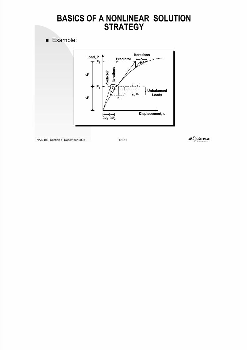
BASICS OF A NONLINEAR SOLUTION
STRATEGY A strategy is required to solve nonlinear problems.
A nonlinear strategy: Advances in increments (example: two load increments). Requires iterations for each increment (example: 5 iterations for the first
increment).
A solution is obtained when the convergence criteria is satisfied
(example: negligibly small unbalanced load).

7/21/2019 Nonlinear Analysis Using MSC.nastran
http://slidepdf.com/reader/full/nonlinear-analysis-using-mscnastran 20/783
S1-16NAS 103, Section 1, December 2003
BASICS OF A NONLINEAR SOLUTION
STRATEGY Example:
Displacement, u
Unbalanced
Loads
P r e
d i c t o r
I t
e r a t i o n s
P2
P1
∆P
∆P
∆u1 ∆u2
R1
R2R3
R4
Load, PPredictor
Iterations

7/21/2019 Nonlinear Analysis Using MSC.nastran
http://slidepdf.com/reader/full/nonlinear-analysis-using-mscnastran 21/783
S1-17NAS 103, Section 1, December 2003
BASICS OF A NONLINEAR SOLUTION
STRATEGY In MSC.NASTRAN
A number of different advancing schemes are available.
A number of different iteration schemes are available. A number of different convergence criteria are available.
User interface: NLPARM Solution strategy for nonlinear static analysis.
SPCD, SPC Displacement increments for nonlinear staticanalysis.
NLPCI Arc length increments for nonlinear static analysis.
TSTEPNL Solution strategy for nonlinear transient analysis.
7/21/2019 Nonlinear Analysis Using MSC.nastran
http://slidepdf.com/reader/full/nonlinear-analysis-using-mscnastran 22/783
S1-18NAS 103, Section 1, December 2003
USER INTERFACE FOR NONLINEAR
ANALYSIS Compatible with linear analysis
Analysis types Nonlinear static analysis: SOL 106 Quasi-static (creep) analysis: SOL 106
Linear buckling analysis: SOL 105
Nonlinear buckling analysis: SOL 106 (PARAM,BUCKLE)
Nonlinear transient response analysis: SOL 129
Subcase structure Allows changes in loads, boundary conditions, and methods.
Allows changes in output requests.
7/21/2019 Nonlinear Analysis Using MSC.nastran
http://slidepdf.com/reader/full/nonlinear-analysis-using-mscnastran 23/783
S1-19NAS 103, Section 1, December 2003
USER INTERFACE FOR NONLINEAR
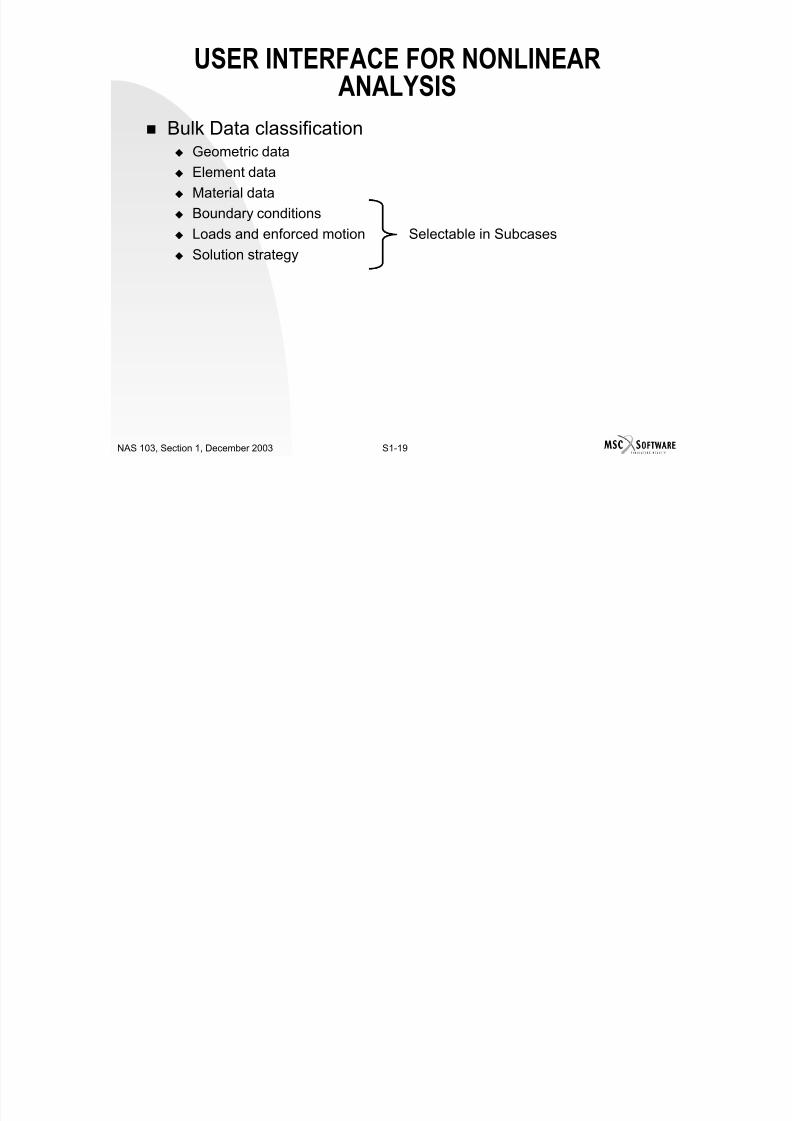
ANALYSIS Bulk Data classification
Geometric data
Element data Material data
Boundary conditions
Loads and enforced motion Selectable in Subcases
Solution strategy

7/21/2019 Nonlinear Analysis Using MSC.nastran
http://slidepdf.com/reader/full/nonlinear-analysis-using-mscnastran 24/783
S1-20NAS 103, Section 1, December 2003
SUMMARY
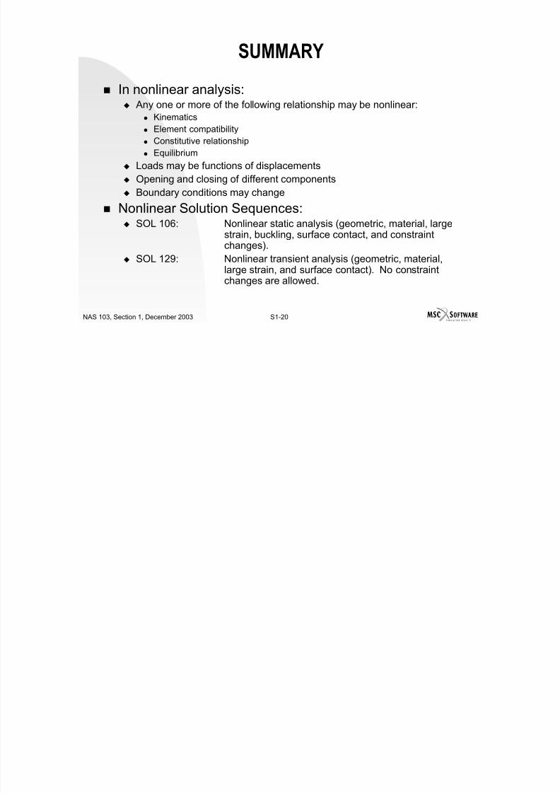
In nonlinear analysis: Any one or more of the following relationship may be nonlinear:
Kinematics Element compatibility Constitutive relationship Equilibrium
Loads may be functions of displacements
Opening and closing of different components Boundary conditions may change
Nonlinear Solution Sequences: SOL 106: Nonlinear static analysis (geometric, material, large
strain, buckling, surface contact, and constraint
changes). SOL 129: Nonlinear transient analysis (geometric, material,
large strain, and surface contact). No constraintchanges are allowed.

7/21/2019 Nonlinear Analysis Using MSC.nastran
http://slidepdf.com/reader/full/nonlinear-analysis-using-mscnastran 25/783
S1-21NAS 103, Section 1, December 2003
SUMMARY
Basic User Interface: Solution strategy:
Solution strategy nonlinear static analysis. NLPARM Arc length increments for nonlinear static analysis. NLPCI
Solution strategy nonlinear transient analysis. TSTEPNL
Displacement-increment analysis. SPCD, SPC
Nonlinear materials: Nonlinear elastic and plastic. MATS1
Creep materials. CREEP
Hyper elastic (rubber-like) materials. MATHP
Temperature-dependent elastic materials. MATT1, MATT2, MATT9 Temperature-dependent
nonlinear elastic materials. TABLEST, TABLES1

7/21/2019 Nonlinear Analysis Using MSC.nastran
http://slidepdf.com/reader/full/nonlinear-analysis-using-mscnastran 26/783
S1-22NAS 103, Section 1, December 2003
SUMMARY
Geometric nonlinear: PARAM, LGDISP.
Follower forces: FORCE1, FORCE2, MOMENT1,MOMENT2, PLOAD, PLOAD2,
PLOADX1, and RFORCE. Nonlinear buckling analysis: PARAM, BUCKLE, in SOL 106.
Contact (interface): gap and 3-D slideline contact.
Boundary changes: SPC, SPCD, and MPC.

7/21/2019 Nonlinear Analysis Using MSC.nastran
http://slidepdf.com/reader/full/nonlinear-analysis-using-mscnastran 27/783
S2-1NAS 103, Section 2, December 2003
SECTION 2
NONLINEAR STATIC ANALYSISSTRATEGIES
7/21/2019 Nonlinear Analysis Using MSC.nastran
http://slidepdf.com/reader/full/nonlinear-analysis-using-mscnastran 28/783
S2-2NAS 103, Section 2, December 2003

7/21/2019 Nonlinear Analysis Using MSC.nastran
http://slidepdf.com/reader/full/nonlinear-analysis-using-mscnastran 29/783
S2-3NAS 103, Section 2, December 2003
TABLE OF CONTENTS
Page
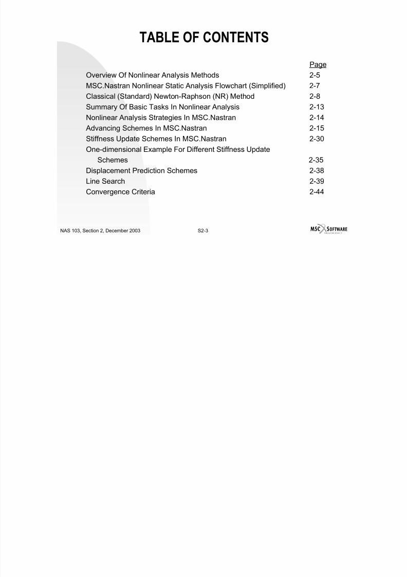
Overview Of Nonlinear Analysis Methods 2-5
MSC.Nastran Nonlinear Static Analysis Flowchart (Simplified) 2-7
Classical (Standard) Newton-Raphson (NR) Method 2-8
Summary Of Basic Tasks In Nonlinear Analysis 2-13
Nonlinear Analysis Strategies In MSC.Nastran 2-14
Advancing Schemes In MSC.Nastran 2-15
Stiffness Update Schemes In MSC.Nastran 2-30
One-dimensional Example For Different Stiffness Update
Schemes 2-35
Displacement Prediction Schemes 2-38
Line Search 2-39Convergence Criteria 2-44
7/21/2019 Nonlinear Analysis Using MSC.nastran
http://slidepdf.com/reader/full/nonlinear-analysis-using-mscnastran 30/783
S2-4NAS 103, Section 2, December 2003
TABLE OF CONTENTS
Page
Special Logics 2-50
Restarts 2-53
Output For Solution Strategies 2-61
Result Output 2-66
Some Heuristic Observations 2-67
Hints And Recommendations 2-68
NLPARM Bulk Data Entry 2-69
Summary 2-70
Workshop Problems 2-73
Solution For Workshop Problem One 2-76
Solution For Workshop Problem Two 2-77

7/21/2019 Nonlinear Analysis Using MSC.nastran
http://slidepdf.com/reader/full/nonlinear-analysis-using-mscnastran 31/783
S2-5NAS 103, Section 2, December 2003
OVERVIEW OF NONLINEAR ANALYSIS
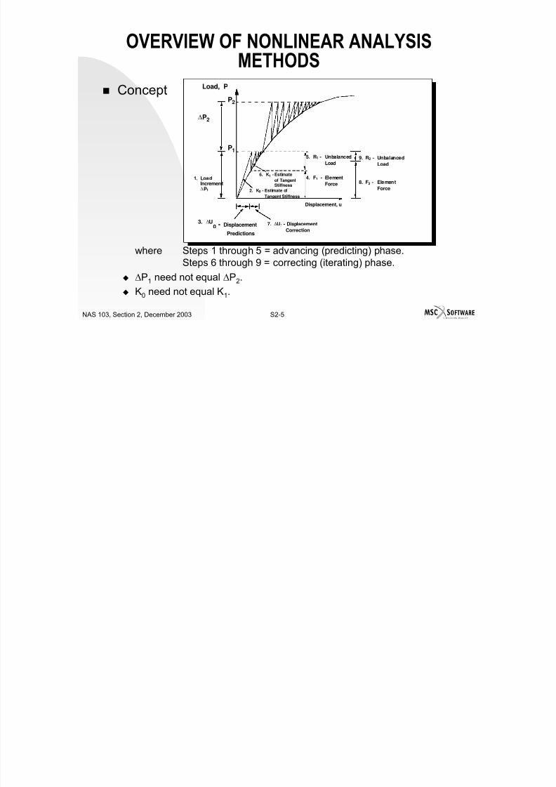
METHODS Concept
where Steps 1 through 5 = advancing (predicting) phase.Steps 6 through 9 = correcting (iterating) phase.
∆P1 need not equal ∆P2.
K0 need not equal K1.
2. K0 - Estimate of
Tangent Stiffness
6. K1 - Estimate
of TangentStiffness
5. R1 - Unbalanced
Load
4. F1 - Element
Force 8. F2 - ElementForce
9. R2 - Unbalanced
Load
Displacement, u
7. ∆U1 - Displacement
Correction
1. Load
Increment∆P1
∆P2
P2
P1
Load, P
3. ∆U0 - Displacement
Predictions
7/21/2019 Nonlinear Analysis Using MSC.nastran
http://slidepdf.com/reader/full/nonlinear-analysis-using-mscnastran 32/783
S2-6NAS 103, Section 2, December 2003
OVERVIEW OF NONLINEAR ANALYSIS
METHODS Algorithm
1. Determine an increment (e.g., load, displacement, or arc length) to move forwardon the equilibrium path.
2. Determine an estimate of a tangent stiffness matrix.3. Determine the displacement increment to move forward, generally by solving
equilibrium equations.4. Calculate the element resisting forces.5. Calculate the unbalanced load and check for convergence. If converged, go to
Step 1.
If not converged, continue as follows:6. Determine an estimate of tangent stiffness matrix.7. Determine the displacement increment due to the unbalanced load.8. Calculate the element resisting forces.9.
Calculate the unbalanced load and check for convergence. If converged, go toStep 1. If not converged, go to Step 6.
Steps 1 through 5 are called the advancing phase or predictingphase.
Steps 6 through 9 are called the correcting phase or iterating phase.

7/21/2019 Nonlinear Analysis Using MSC.nastran
http://slidepdf.com/reader/full/nonlinear-analysis-using-mscnastran 33/783
S2-7NAS 103, Section 2, December 2003
MSC.NASTRAN NONLINEAR STATIC
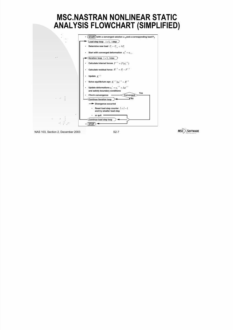
ANALYSIS FLOWCHART (SIMPLIFIED)• START with a converged solution u 0 and a corresponding load P0
Load step loop l = 1, l step
• Determine new load
• Start with converged deformation
Iteration loop i = 1, i max
• Calculate internal forces
• Calculate residual force:
• Update
• Solve equilibrium eqn:
• Update deformations
and satisfy boundary conditions
• Check convergence Converged
Continue iteration loop
Divergence occurred
• Reset load step counter
and try smaller load step
• or quit
Continue load step loop
• STOP
Yes
No
l l l P P P ∆+= −1
10 −= l l uu
)( 11 −− = i
l
i u F F
11 −− −= i
l
i F P R
1−i
K 111 −−− =∆ iii
Ru K
11 −− ∆+= ii
l
i
l uuu
1−= l l
7/21/2019 Nonlinear Analysis Using MSC.nastran
http://slidepdf.com/reader/full/nonlinear-analysis-using-mscnastran 34/783
S2-8NAS 103, Section 2, December 2003
CLASSICAL (STANDARD) NEWTON-RAPHSON
(NR) METHOD Advance forward by constant and positive load increments.
Tangent stiffness is formed at every iteration.
Displacement is predicted and corrected by solving equilibriumequations.

7/21/2019 Nonlinear Analysis Using MSC.nastran
http://slidepdf.com/reader/full/nonlinear-analysis-using-mscnastran 35/783
S2-9NAS 103, Section 2, December 2003
CLASSICAL (STANDARD) NEWTON-RAPHSON
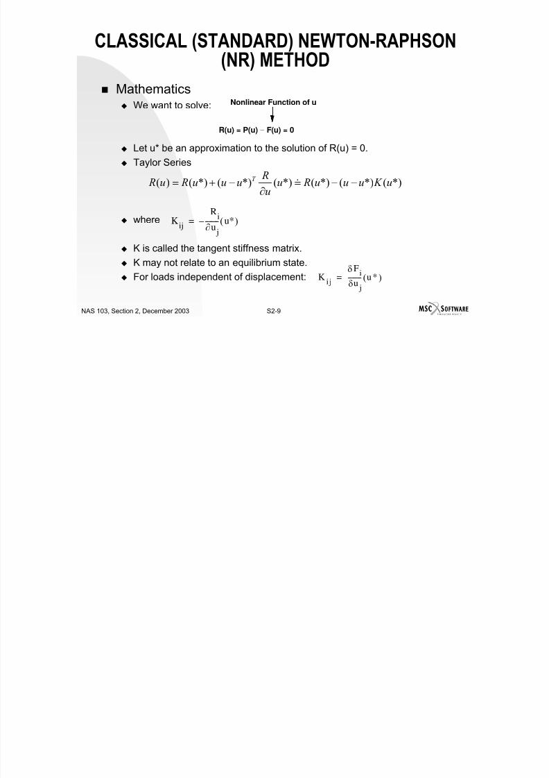
(NR) METHOD Mathematics
We want to solve:
Let u* be an approximation to the solution of R(u) = 0.
Taylor Series
where
K is called the tangent stiffness matrix.
K may not relate to an equilibrium state.
For loads independent of displacement:
R(u) = P(u) − F(u) = 0
Nonlinear Function of u
Kij
Ri
∂u j
-------- u*( )–=
Ki j
δ Fi
δu j
-------- u *( )=
*)(*)(*)(*)(*)(*)()( u K uuu Ruu
Ruuu Ru R T −−=∂−+= &
7/21/2019 Nonlinear Analysis Using MSC.nastran
http://slidepdf.com/reader/full/nonlinear-analysis-using-mscnastran 36/783
S2-10NAS 103, Section 2, December 2003
CLASSICAL (STANDARD) NEWTON-RAPHSON
(NR) METHOD Algorithm
Solve:
Solve:
Solve:
until reaching convergence
Note: At each iteration, tangent K is computed from the currentelement state.
K u0
( )∆u0
P F0
∆R u0
( )==
u1 u0 ∆u0+=
K u1
( ) ∆ u1
R u1
( )=
u2
u1
∆u1
+=
K u 2( ) ∆ u 2 R u 2( )=
u3
u2
∆u2
+=
.
.
.

7/21/2019 Nonlinear Analysis Using MSC.nastran
http://slidepdf.com/reader/full/nonlinear-analysis-using-mscnastran 37/783
S2-11NAS 103, Section 2, December 2003
CLASSICAL (STANDARD) NEWTON-RAPHSON
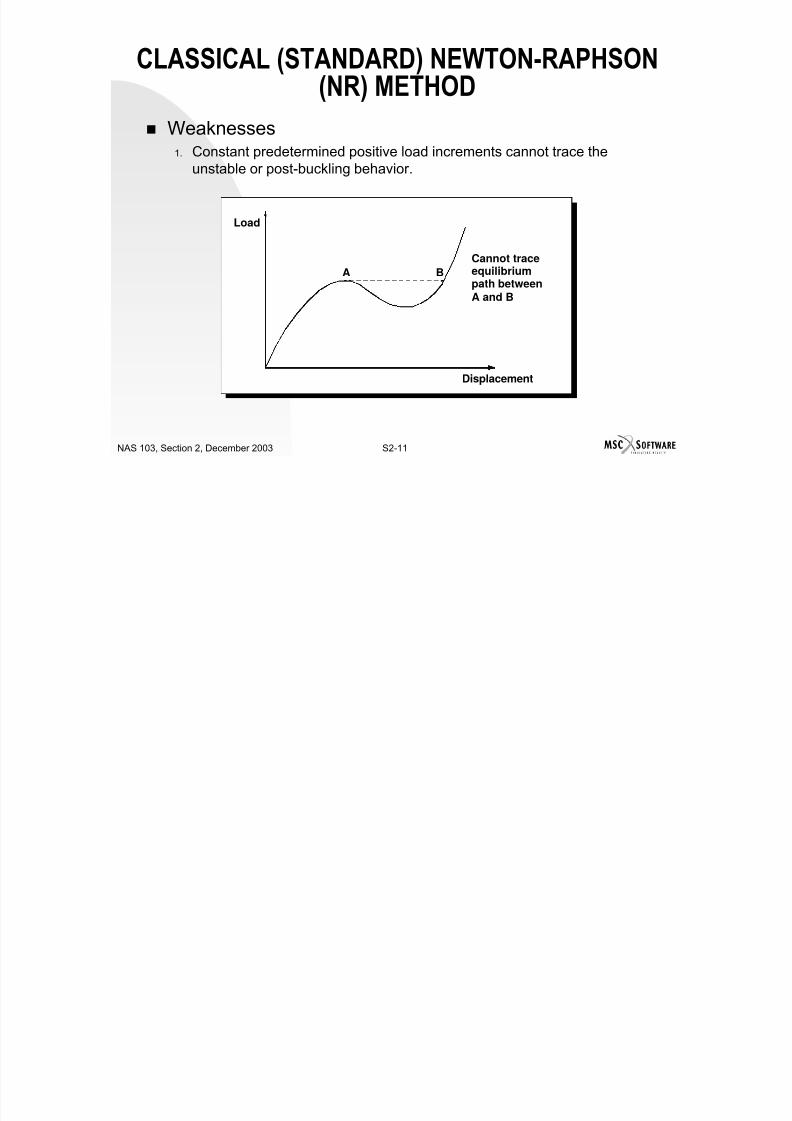
(NR) METHOD Weaknesses
1. Constant predetermined positive load increments cannot trace theunstable or post-buckling behavior.
Displacement
Load
Cannot traceequilibriumpath betweenA and B
A B

7/21/2019 Nonlinear Analysis Using MSC.nastran
http://slidepdf.com/reader/full/nonlinear-analysis-using-mscnastran 38/783
S2-12NAS 103, Section 2, December 2003
CLASSICAL (STANDARD) NEWTON-RAPHSON
(NR) METHOD2. No convergence if total applied load is greater than the structure
strength.
3. Computation of tangent stiffness at each iteration is expensive and
unnecessary when the solution is close to convergence.4. Path-dependent state determination. Use of nonconverged reference
state may cause the inelastic material response to differ from the trueresponse.
5. Special logic is necessary if solution does not converge.
No Solution
Displacement
P
∆P4
∆P3
∆P2
∆P1

7/21/2019 Nonlinear Analysis Using MSC.nastran
http://slidepdf.com/reader/full/nonlinear-analysis-using-mscnastran 39/783
S2-13NAS 103, Section 2, December 2003
SUMMARY OF BASIC TASKS IN NONLINEAR
ANALYSIS1. Determination of an increment to advance forward on
the equilibrium path.
2. Determination of an estimate of tangent stiffness matrix.3. Prediction of the displacement for the increment.
4. Determination of the element state: deformation,
resisting forces, etc.5. Convergence check. Calculation of unbalanced forces
and satisfaction of convergence criteria.

7/21/2019 Nonlinear Analysis Using MSC.nastran
http://slidepdf.com/reader/full/nonlinear-analysis-using-mscnastran 40/783
S2-14NAS 103, Section 2, December 2003
NONLINEAR ANALYSIS STRATEGIES IN
MSC.NASTRAN Different schemes are available for advancing forward on
the equilibrium path.
Different schemes are available for estimating thetangent stiffness.
Different schemes are available for predicting thedisplacement increment.
Different convergence criteria are available. Note: Users can select different solution strategies based on
different combination of schemes selected for different tasks

7/21/2019 Nonlinear Analysis Using MSC.nastran
http://slidepdf.com/reader/full/nonlinear-analysis-using-mscnastran 41/783
S2-15NAS 103, Section 2, December 2003
ADVANCING SCHEMES IN MSC.NASTRAN
Constant load increments
Constant displacement increments
Arc-length increments
7/21/2019 Nonlinear Analysis Using MSC.nastran
http://slidepdf.com/reader/full/nonlinear-analysis-using-mscnastran 42/783
S2-16NAS 103, Section 2, December 2003
ADVANCING SCHEMES IN MSC.NASTRAN
Constant Load Increment
Field ContentsID Identification number. (Integer > 0).NINC Number of increments. (0 < Integer < 1000).
Example:
SUBCASE = 10NLPARM = 10LOAD = 10BEGIN BULK
NLPARM,10,5FORCE,10,1,,100.,1.,0.,0.FORCE,10,3,,300.,0.,1.,0.MOMENT,10,6,,100.,0.,0.,1.
..
NINCIDNLPARM
10987654321
.
.

7/21/2019 Nonlinear Analysis Using MSC.nastran
http://slidepdf.com/reader/full/nonlinear-analysis-using-mscnastran 43/783
S2-17NAS 103, Section 2, December 2003
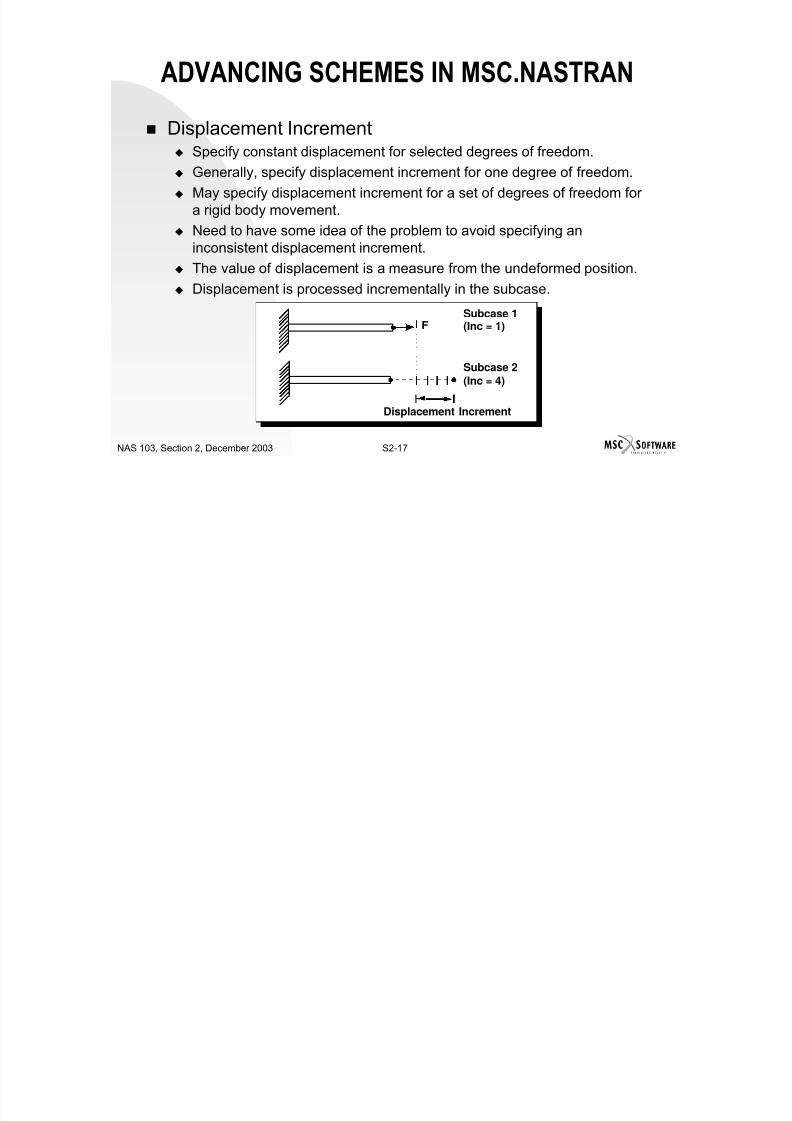
ADVANCING SCHEMES IN MSC.NASTRAN
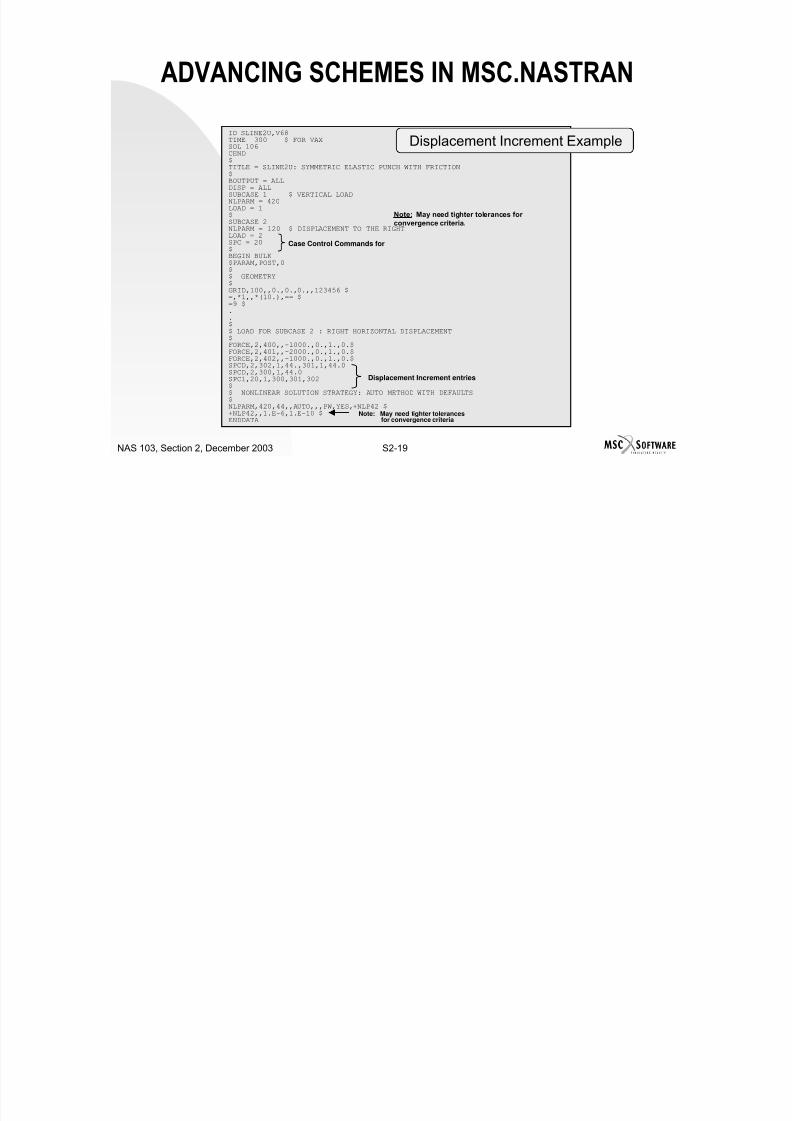
Displacement Increment Specify constant displacement for selected degrees of freedom.
Generally, specify displacement increment for one degree of freedom. May specify displacement increment for a set of degrees of freedom for
a rigid body movement.
Need to have some idea of the problem to avoid specifying aninconsistent displacement increment.
The value of displacement is a measure from the undeformed position. Displacement is processed incrementally in the subcase.
F
Displacement Increment
Subcase 1(Inc = 1)
Subcase 2
(Inc = 4)
7/21/2019 Nonlinear Analysis Using MSC.nastran
http://slidepdf.com/reader/full/nonlinear-analysis-using-mscnastran 44/783
S2-18NAS 103, Section 2, December 2003
ADVANCING SCHEMES IN MSC.NASTRAN
May need tighter tolerances than the default for convergence criteria.
May be used in combination with load increment.
Cannot be used in combination with arc-length increments.
Specified in the Bulk Data entry SPCD or SPC.
If specified in Bulk Data entry SPCD: Selected by LOAD in Case Control.
SPCD cannot be combined in the Bulk Data LOAD.
The degree of freedom with the SPCD should be defined in theS-set (SPC).
Appropriate S-set should be selected in the subcase.
7/21/2019 Nonlinear Analysis Using MSC.nastran
http://slidepdf.com/reader/full/nonlinear-analysis-using-mscnastran 45/783
S2-19NAS 103, Section 2, December 2003
ADVANCING SCHEMES IN MSC.NASTRAN
ID SLINE2U,V68TIME 300 $ FOR VAXSOL 106CEND$TITLE = SLINE2U: SYMMETRIC ELASTIC PUNCH WITH FRICTION$BOUTPUT = ALLDISP = ALLSUBCASE 1 $ VERTICAL LOADNLPARM = 420LOAD = 1$SUBCASE 2NLPARM = 120 $ DISPLACEMENT TO THE RIGHTLOAD = 2SPC = 20$BEGIN BULK
$PARAM,POST,0$$ GEOMETRY$GRID,100,,0.,0.,0.,,123456 $=,*1,,*(10.),== $=9 $..$$ LOAD FOR SUBCASE 2 : RIGHT HORIZONTAL DISPLACEMENT$FORCE,2,400,,-1000.,0.,1.,0.$FORCE,2,401,,-2000.,0.,1.,0.$FORCE,2,402,,-1000.,0.,1.,0.$SPCD,2,302,1,44.,301,1,44.0SPCD,2,300,1,44.0SPC1,20,1,300,301,302$$ NONLINEAR SOLUTION STRATEGY: AUTO METHOD WITH DEFAULTS$NLPARM,420,44,,AUTO,,,PW,YES,+NLP42 $+NLP42,,1.E-6,1.E-10 $ENDDATA
Displacement Increment Example
Note: May need tighter tolerances forconvergence criteria.
Displacement Increment entries
Note: May need tighter tolerancesfor convergence criteria
Case Control Commands for
7/21/2019 Nonlinear Analysis Using MSC.nastran
http://slidepdf.com/reader/full/nonlinear-analysis-using-mscnastran 46/783
7/21/2019 Nonlinear Analysis Using MSC.nastran
http://slidepdf.com/reader/full/nonlinear-analysis-using-mscnastran 47/783
S2-21NAS 103, Section 2, December 2003
ADVANCING SCHEMES IN MSC.NASTRAN
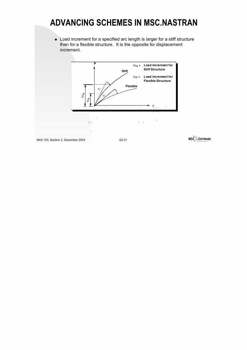
Load increment for a specified arc length is larger for a stiff structurethan for a flexible structure. It is the opposite for displacementincrement.
P
Stiff
Flexible
∆µs = Load Increment for
Stiff Structure
∆µf = Load Increment for
Flexible Structure
∆l
∆l
∆ µ f ∆
µ s
µ
7/21/2019 Nonlinear Analysis Using MSC.nastran
http://slidepdf.com/reader/full/nonlinear-analysis-using-mscnastran 48/783
7/21/2019 Nonlinear Analysis Using MSC.nastran
http://slidepdf.com/reader/full/nonlinear-analysis-using-mscnastran 49/783
S2-23NAS 103, Section 2, December 2003
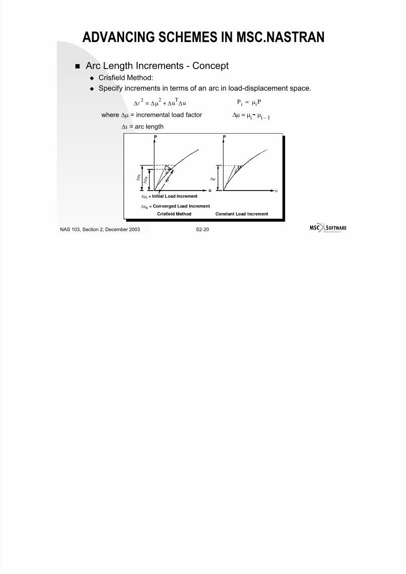
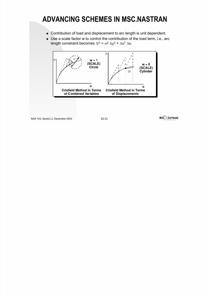
ADVANCING SCHEMES IN MSC.NASTRAN
Contribution of load and displacement to arc length is unit dependent.
Use a scale factor w to control the contribution of the load term, i.e., arclength constraint becomes ∆l2 = ω2 ∆µ2 + ∆uT ∆u.
µ
u u
µ
Crisfield Method in Terms
of Combined Variables
Crisfield Method in Terms
of Displacements
w = 1(SCALE)
Circle
∆l
w = 0(SCALE)Cylinder
∆l
7/21/2019 Nonlinear Analysis Using MSC.nastran
http://slidepdf.com/reader/full/nonlinear-analysis-using-mscnastran 50/783
S2-24NAS 103, Section 2, December 2003
ADVANCING SCHEMES IN MSC.NASTRAN
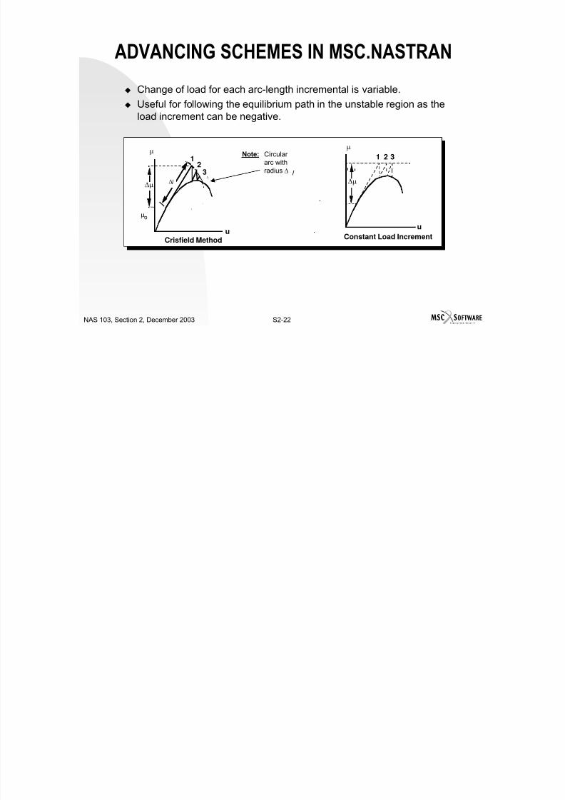
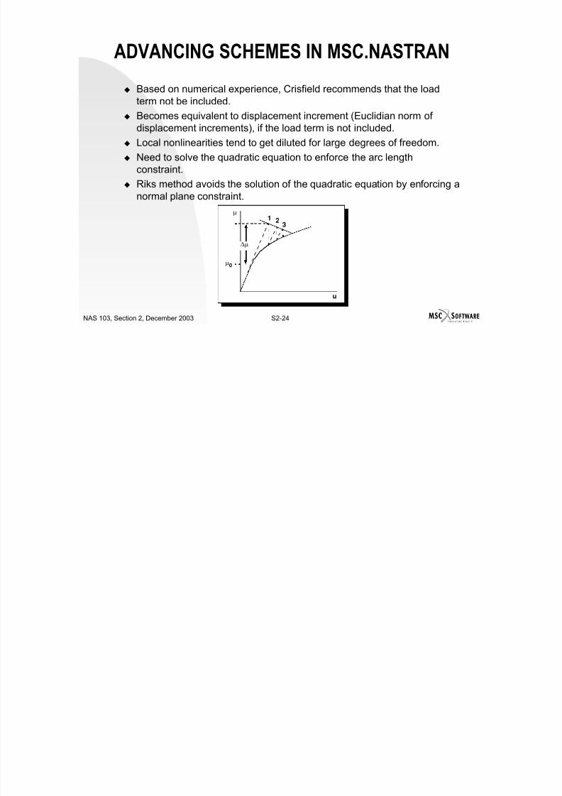
Based on numerical experience, Crisfield recommends that the loadterm not be included.
Becomes equivalent to displacement increment (Euclidian norm of
displacement increments), if the load term is not included. Local nonlinearities tend to get diluted for large degrees of freedom.
Need to solve the quadratic equation to enforce the arc lengthconstraint.
Riks method avoids the solution of the quadratic equation by enforcing anormal plane constraint.
µ1 2
3
∆µ
µ0
u
7/21/2019 Nonlinear Analysis Using MSC.nastran
http://slidepdf.com/reader/full/nonlinear-analysis-using-mscnastran 51/783
S2-25NAS 103, Section 2, December 2003
ADVANCING SCHEMES IN MSC.NASTRAN
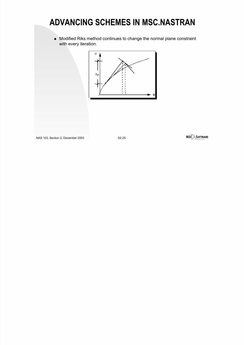
Modified Riks method continues to change the normal plane constraintwith every iteration.
∆µ
µ
u

7/21/2019 Nonlinear Analysis Using MSC.nastran
http://slidepdf.com/reader/full/nonlinear-analysis-using-mscnastran 52/783
S2-26NAS 103, Section 2, December 2003
ADVANCING SCHEMES IN MSC.NASTRAN
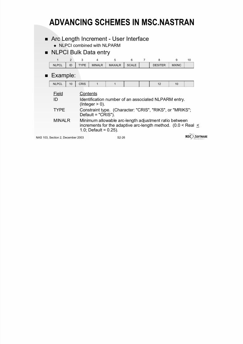
Arc Length Increment - User Interface NLPCI combined with NLPARM
NLPCI Bulk Data entry
Example:
Field ContentsID Identification number of an associated NLPARM entry.
(Integer > 0).
TYPE Constraint type. (Character: "CRIS", "RIKS", or "MRIKS";Default = "CRIS").
MINALR Minimum allowable arc-length adjustment ratio betweenincrements for the adaptive arc-length method. (0.0 < Real <1.0; Default = 0.25).
MXINCDESITERSCALEMAXALRMINALRTYPEIDNLPCL
10987654321
101211CRIS10NLPCL
ADVANCING SCHEMES IN MSC NASTRAN

7/21/2019 Nonlinear Analysis Using MSC.nastran
http://slidepdf.com/reader/full/nonlinear-analysis-using-mscnastran 53/783
S2-27NAS 103, Section 2, December 2003
ADVANCING SCHEMES IN MSC.NASTRAN
Field Contents
MAXALR Maximum allowable arc-length adjustment ratio betweenincrements for the adaptive arc-length method. (Real > 1.0;
Default = 4.0).SCALE Scale factor (w) for controlling the loading contribution in the
arc-length constraint. (Real > 0.0; Default = 0.0)
DESITER Desired number of iterations for convergence to be used forthe adaptive arc-length adjustment. (Integer > 0; Default =12).
MXINC Maximum number of controlled increment steps allowedwithin a subcase. (Integer > 0; Default = 20).
ADVANCING SCHEMES IN MSC NASTRAN

7/21/2019 Nonlinear Analysis Using MSC.nastran
http://slidepdf.com/reader/full/nonlinear-analysis-using-mscnastran 54/783
S2-28NAS 103, Section 2, December 2003
ADVANCING SCHEMES IN MSC.NASTRAN
NLPARM Bulk Data Entry
Field Contents
MAXR Maximum ratio for the adjusted arc-length increment relativeto the initial value. (1.0 ≤ MAXR ≤ 40.0; Default = 20.0).
Example: NLPARM = 20
BEGIN BULKNLPARM,20,10NLPCI,20,CRIS,1.,1.,,,12,40ENDDATA
MAXR
IDNLPARM
10987654321
ADVANCING SCHEMES IN MSC NASTRAN

7/21/2019 Nonlinear Analysis Using MSC.nastran
http://slidepdf.com/reader/full/nonlinear-analysis-using-mscnastran 55/783
S2-29NAS 103, Section 2, December 2003
ADVANCING SCHEMES IN MSC.NASTRAN
Option to specify either Crisfield, Riks, or modified Riksmethods.
Must be used in combination with a load increment, Initial arc length is based on the load increment specified
in NLPARM Bulk Data entry.
Can vary arc length based on the number of iterations.
Recommendation: Use constant arc length increments.
Disallowed with displacement increments (SPCD).
Line search* is not operational with arc lengthincrements.
Not allowed for creep analysis**Note: Will be discussed later on.
STIFFNESS UPDATE SCHEMES IN

7/21/2019 Nonlinear Analysis Using MSC.nastran
http://slidepdf.com/reader/full/nonlinear-analysis-using-mscnastran 56/783
S2-30NAS 103, Section 2, December 2003
STIFFNESS UPDATE SCHEMES IN
MSC.NASTRAN At every iteration (NR method)
At every k-th iteration (modified NR method)
Based on the rate of convergence. Logic is hardwaredependent. For the same problem, the solution pathmay be different depending on the hardware.
On non-convergence or divergence
Quasi-Newton stiffness updates
MAXQN
MAXITERKSTEPKMETHODIDNLPARM
10987654321
STIFFNESS UPDATE SCHEMES IN

7/21/2019 Nonlinear Analysis Using MSC.nastran
http://slidepdf.com/reader/full/nonlinear-analysis-using-mscnastran 57/783
S2-31NAS 103, Section 2, December 2003
STIFFNESS UPDATE SCHEMES IN
MSC.NASTRANField Contents
KMETHOD Method for controlling stiffness updates. (Character ="AUTO", "ITER", or "SEMI"; Default = "AUTO").
KSTEP Number of iterations before the stiffness update for ITERmethod. (Integer > 1; Default = 5).
MAXITER Limit on number of iterations for each load increment.(Integer > 0; Default = 25).
MAXQN Maximum number of quasi-Newton correction vectors to besaved on the database. (Integer > 0; Default = MAXITER).
STIFFNESS UPDATE SCHEMES IN
7/21/2019 Nonlinear Analysis Using MSC.nastran
http://slidepdf.com/reader/full/nonlinear-analysis-using-mscnastran 58/783
S2-32NAS 103, Section 2, December 2003
S SS U SC S
MSC.NASTRAN Quasi-Newton (QN) Stiffness Updates – Concept
Full Newton-Raphson is very expensive.
Modified Newton-Raphson converges slowly, if at all.
Hence we seek a simple but efficient way to update (rather than recompute) thestiffness, after each iteration.
Modified stiffness matrix should be a secant stiffness matrix for thedisplacements calculated in the previous iterations.
Modified stiffness should preserve symmetry and be positive definite.
Displacement increment using modified stiffness should be inexpensive tocalculate.
STIFFNESS UPDATE SCHEMES IN
7/21/2019 Nonlinear Analysis Using MSC.nastran
http://slidepdf.com/reader/full/nonlinear-analysis-using-mscnastran 59/783
S2-33NAS 103, Section 2, December 2003
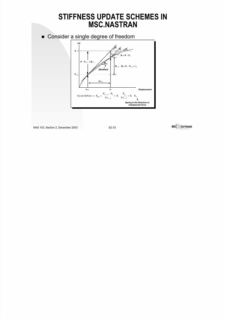
MSC.NASTRAN Consider a single degree of freedom
Km
(Modified)
F,P
K
Spring in the Direction ofUnbalanced Force
u i-1 ui
P
Displacement
K Kt
Ri = P – Fi
Ri–1 – Ri = Fi – Fi–1 = γi
P – Fi–1 = Ri–1
∆ui–1
Secant Stiffness Km
Ri 1– Ri–
∆ui 1–
------------------------- KRi
∆ui 1–
---------------- K Ks–=–= = =
Fi–1
STIFFNESS UPDATE SCHEMES IN
7/21/2019 Nonlinear Analysis Using MSC.nastran
http://slidepdf.com/reader/full/nonlinear-analysis-using-mscnastran 60/783
S2-34NAS 103, Section 2, December 2003
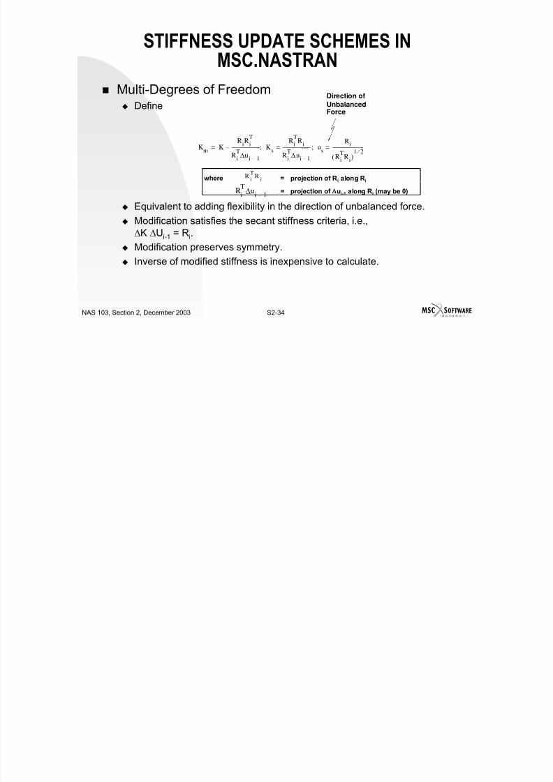
MSC.NASTRAN Multi-Degrees of Freedom
Define
Equivalent to adding flexibility in the direction of unbalanced force.
Modification satisfies the secant stiffness criteria, i.e.,∆K ∆Ui-1 = Ri.
Modification preserves symmetry. Inverse of modified stiffness is inexpensive to calculate.
Km
KR
iR
i
T
Ri
T∆u
i 1–
------------------------; Ks
Ri
TR
i
Ri
T∆u
i 1–
------------------------ ; us
Ri
Ri
TR
i( )
1 2 ⁄ ---------------------------==–=
Direction of
UnbalancedForce
where = projection of Ri along Ri
= projection of ∆ui-1 along Ri (may be 0)
Ri
TR
i
RiT∆u
i 1–
ONE-DIMENSIONAL EXAMPLE FOR

7/21/2019 Nonlinear Analysis Using MSC.nastran
http://slidepdf.com/reader/full/nonlinear-analysis-using-mscnastran 61/783
S2-35NAS 103, Section 2, December 2003
DIFFERENT STIFFNESS UPDATE SCHEMES
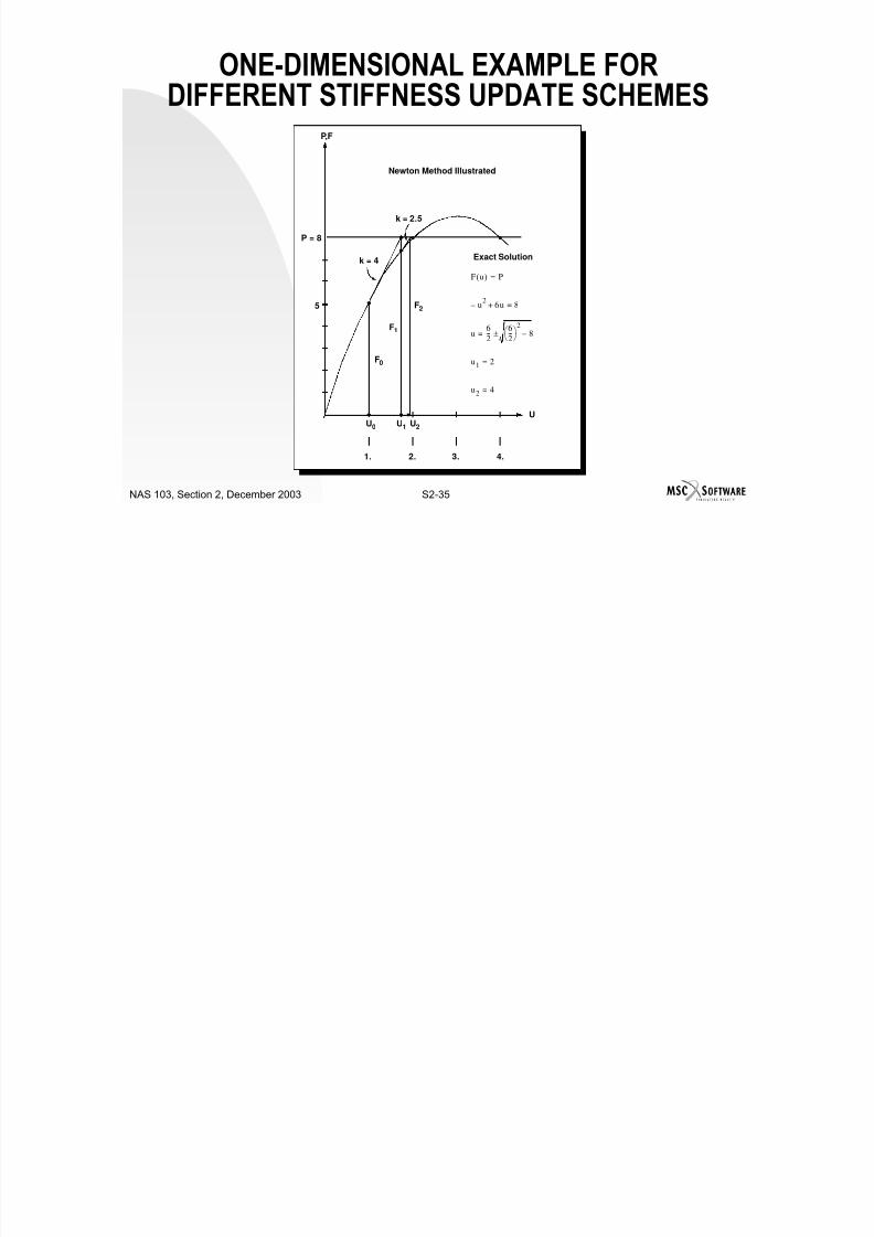
F u( ) P=
u2
– 6u 8=+
u6
2---
6
2---
2
8–±=
u1 2=
u2 4=
1. 2. 3. 4.
U
Newton Method Illustrated
k = 2.5
P,F
P = 8
5
U0 U1 U2
k = 4
F1
F0
F2
Exact Solution
ONE-DIMENSIONAL EXAMPLE FOR

7/21/2019 Nonlinear Analysis Using MSC.nastran
http://slidepdf.com/reader/full/nonlinear-analysis-using-mscnastran 62/783
S2-36NAS 103, Section 2, December 2003
DIFFERENT STIFFNESS UPDATE SCHEMES Convergence Criteria: R < 0.01
Newton Method
Note: Quadratic rate of convergence
Modified Newton Method
Note: Linear rate of convergence.
Iteration Initial U Initial R K U Final U F Final R
1 1.0000 3.0000 4.0000 0.7500 1.7500 7.4375 0.5625
2 1.7500 0.5625 2.5000 0.2250 1.9750 7.9494 0.0506
3 1.9750 0.0506 2.0500 0.0247 1.9997 7.9994 0.0006
Iteration Initial U Initial R K U Final U F Final R
1 1.0000 3.0000 4.0000 0.7500 1.7500 7.4375 0.5625
2 1.7500 0.5625 4.0000 0.1406 1.8906 7.7692 0.2308
3 1.8906 0.2308 4.0000 0.0577 1.9483 7.8939 0.1061
4 1.9483 0.1061 4.0000 0.0265 1.9748 7.9490 0.0510
5 1.9748 0.0510 4.0000 0.0128 1.9876 7.9750 0.02506 1.9876 0.0250 4.0000 0.0063 1.9939 7.9878 0.0122
7 1.9939 0.0122 4.0000 0.0031 1.9970 7.9940 0.0060
ONE-DIMENSIONAL EXAMPLE FOR

7/21/2019 Nonlinear Analysis Using MSC.nastran
http://slidepdf.com/reader/full/nonlinear-analysis-using-mscnastran 63/783
S2-37NAS 103, Section 2, December 2003
DIFFERENT STIFFNESS UPDATE SCHEMES Modified Newton Method with QN Update
Ki = Ki-1 - Ri-1 /∆Ui-1
Iteration Initial U Initial R K U Final U F Final R
1 1.0000 3.0000 4.0000 0.75 1.75 7.4375 0.5625
2 1.7500 0.5625 3.2500 0.1731 1.9231 7.8403 0.1597
3 1.9231 0.1597 2.3274 0.0686 1.9917 7.9833 0.01674 1.9917 0.0167 2.0840 0.008 1.9997 7.9994 0.0006
DISPLACEMENT PREDICTION SCHEMES

7/21/2019 Nonlinear Analysis Using MSC.nastran
http://slidepdf.com/reader/full/nonlinear-analysis-using-mscnastran 64/783
S2-38NAS 103, Section 2, December 2003
DISPLACEMENT PREDICTION SCHEMES
Solution of equilibrium equation
Line search method
LINE SEARCH

7/21/2019 Nonlinear Analysis Using MSC.nastran
http://slidepdf.com/reader/full/nonlinear-analysis-using-mscnastran 65/783
S2-39NAS 103, Section 2, December 2003
LINE SEARCH
Concept Improves displacement increment calculated from the equilibrium
equation.
Displacement increment calculated from the equilibrium equation is notnecessarily the best estimate of the equilibrium state. Seek a multiple of displacement increment (a) that minimizes a measure
of work done by unbalanced forces. Applicable for each iteration.
Effective when the modified Newton method is used. Effective for contact problems. Phase 1: Seek upper and lower values of a that bound zero unbalance.
Calculate a measure of external work done by unbalanced loads for thebeginning of iteration (α0 = 0) and for the calculated displacement increment
(α1 = 1). If the unbalances at α0 and α1 are of opposite signs, the zero is bounded and
then go to phase 2. If the zero is not bounded, keep doubling ∆U until the zero is bounded or the
number of line searches allowed is performed.
LINE SEARCH

7/21/2019 Nonlinear Analysis Using MSC.nastran
http://slidepdf.com/reader/full/nonlinear-analysis-using-mscnastran 66/783
S2-40NAS 103, Section 2, December 2003
LINE SEARCH
Phase 2: Find a to minimize the unbalance. Let αk and αk – 1 be the scalar multiplies that bound the zero unbalance.
Based on the values of αk and αk – 1 , linearly interpolate to get a new value
of α. Evaluate the new unbalance at new a and keep interpolating between the
two a with opposite signs until the unbalance is less than the specifiedproportion of
or
the number of line searches allowed is performed.
αn( ) α0( )<
LINE SEARCH
7/21/2019 Nonlinear Analysis Using MSC.nastran
http://slidepdf.com/reader/full/nonlinear-analysis-using-mscnastran 67/783
S2-41NAS 103, Section 2, December 2003
LINE SEARCH
User Interface
Field Contents
MAXLS Maximum number of line searches allowed for each iteration.(Integer > 0; Default = 4)
LSTOL Line search tolerance. (0.01 ≤ Real ≤ 0.9; Default = 0.5)
LSTOLMAXLS
IDNLPARM
10987654321
LINE SEARCH
7/21/2019 Nonlinear Analysis Using MSC.nastran
http://slidepdf.com/reader/full/nonlinear-analysis-using-mscnastran 68/783
S2-42NAS 103, Section 2, December 2003
LINE SEARCH
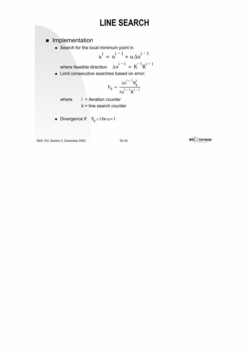
Implementation Search for the local minimum point in
where feasible direction
Limit consecutive searches based on error:
where i = iteration counter
k = line search counter
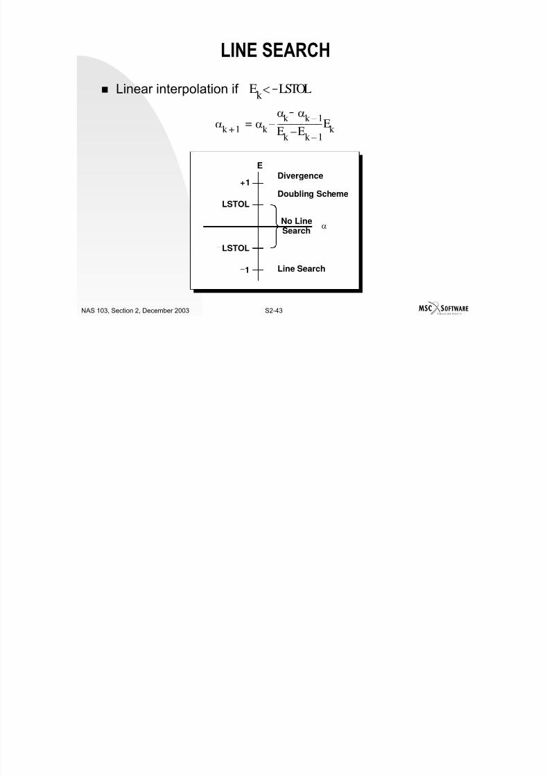
Divergence if Ek
1 for α 1=>
Ek ∆u
i 1
Rk
i
∆ui 1–
Ri 1–
------------------------------=
u
i
u
i 1
α∆u
i 1
+=
∆ui 1
K1R
i 1=
LINE SEARCH

7/21/2019 Nonlinear Analysis Using MSC.nastran
http://slidepdf.com/reader/full/nonlinear-analysis-using-mscnastran 69/783
S2-43NAS 103, Section 2, December 2003
S C
Linear interpolation if
−LSTOL
LSTOL
+1
−1
E
No LineSearch
Divergence
Doubling Scheme
Line Search
α
Ek
LSTOL<
αk 1+ αk
αk
αk 1–
Ek Ek 1––--------------------------Ek –=
CONVERGENCE CRITERIA
7/21/2019 Nonlinear Analysis Using MSC.nastran
http://slidepdf.com/reader/full/nonlinear-analysis-using-mscnastran 70/783
S2-44NAS 103, Section 2, December 2003
Criteria should: Be satisfied for the linear case at all times.
Be independent of structural units.
Be reliable and consistent; no cancellation errors.
Be independent of structural characteristics.
Be applicable to all loading cases
Have smooth transition after K updates and loading changes.
Be dimensionless.
Three criteria: Load (Ep) Work (Ew)
Displacement (Eu)
P = 0; ∆P = 0 (creep)
CONVERGENCE CRITERIA

7/21/2019 Nonlinear Analysis Using MSC.nastran
http://slidepdf.com/reader/full/nonlinear-analysis-using-mscnastran 71/783
S2-45NAS 103, Section 2, December 2003
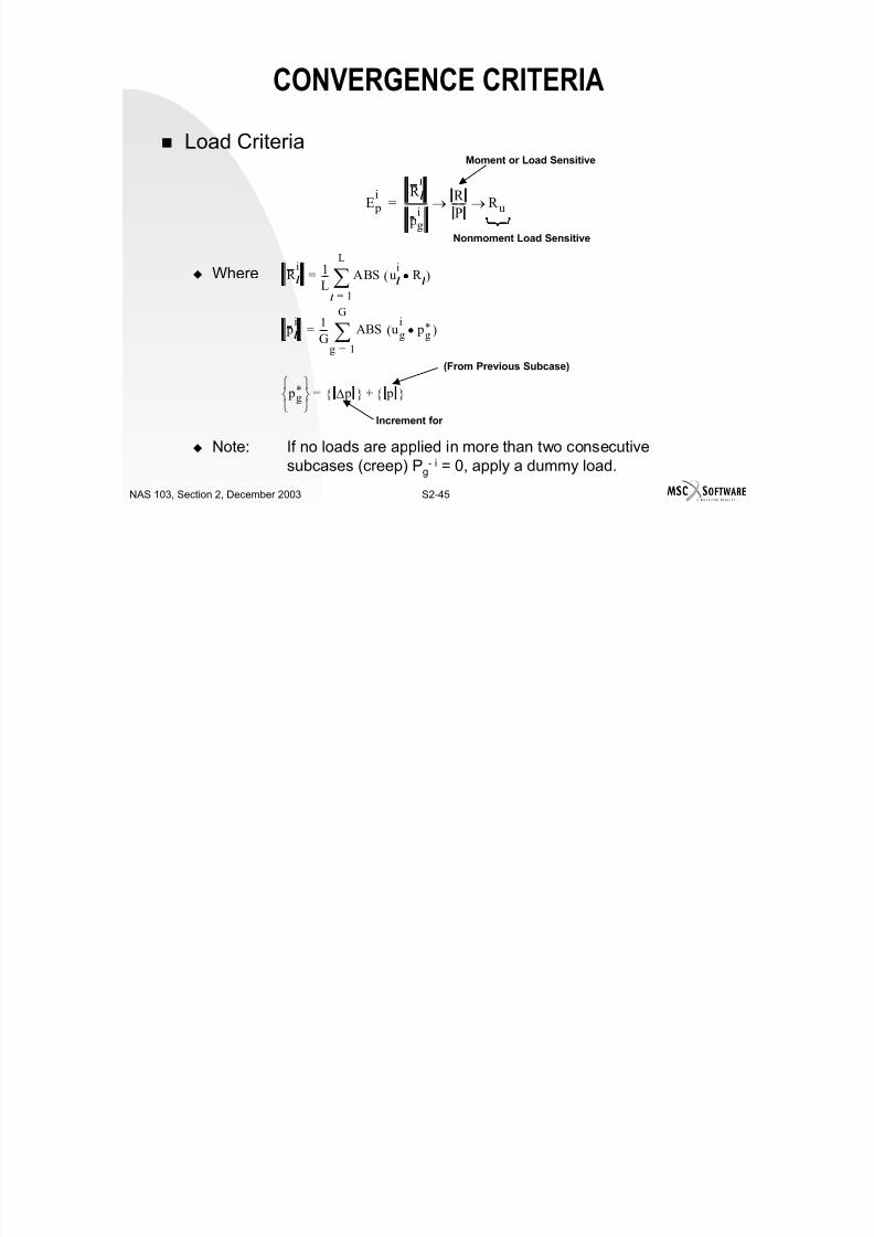
Load Criteria
Where
Note: If no loads are applied in more than two consecutivesubcases (creep) Pg
- i = 0, apply a dummy load.
R l
i 1
L--- ABS
l 1=
L
∑ ul
iR l
•( )=
pl
i 1
G---- ABS
g 1=
G
∑ ug
i pg
*•( )=
pg*
∆ p p +=
Increment for
(From Previous Subcase)
Moment or Load Sensitive
Nonmoment Load Sensitive
E p
i R l
pgi----------
R
P------ R u→ →=
CONVERGENCE CRITERIA
7/21/2019 Nonlinear Analysis Using MSC.nastran
http://slidepdf.com/reader/full/nonlinear-analysis-using-mscnastran 72/783
S2-46NAS 103, Section 2, December 2003
Work Criteria
Where
Note: If no loads are applied in more than two consecutivesubcases (creep) Pg
- i = 0, apply a dummy load.
LineSearch
Ew
i
α Rl
i
∆ul
i 1–
•
pg
i-------------------------------------------------=
R l
i
∆Ul
i 1 –
• 1
L--- ABS
l 1=
L
∑ R l
i∆U
l
i 1 – •( )=
CONVERGENCE CRITERIA

7/21/2019 Nonlinear Analysis Using MSC.nastran
http://slidepdf.com/reader/full/nonlinear-analysis-using-mscnastran 73/783
S2-47NAS 103, Section 2, December 2003
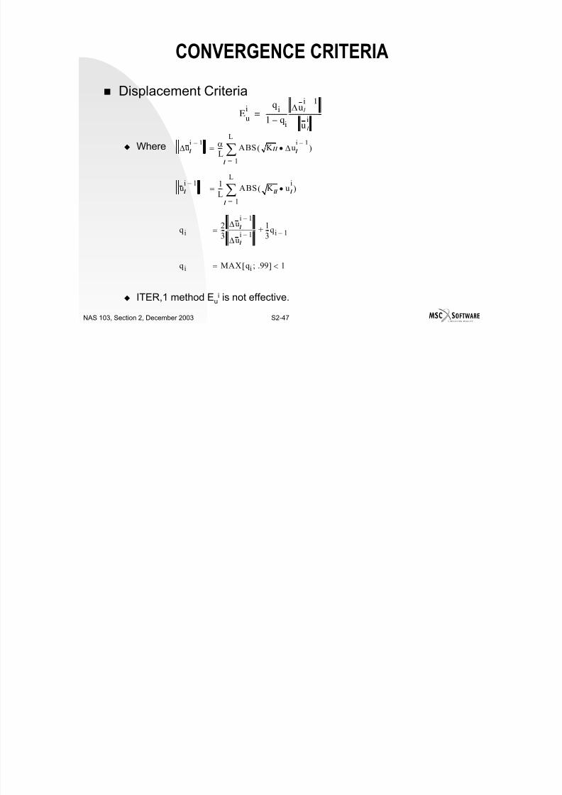
Displacement Criteria
Where
ITER,1 method Eui is not effective.
Eu
i qi
1 qi
–-------------
∆ul
i 1
ul
i---------------------=
ul
i 1 –
=
1
L--- ABS K ll u l
i
•( )l 1=
L
∑
qi = 2
3---
∆ul
i 1 –
∆ul
i 1 – ---------------------
1
3---qi 1 – +
qi = MAX qi .99;[ ] 1<
∆ul
i 1 – = α
L--- ABS K l l ∆u
l
i 1 – •( )
l 1=
L
∑
CONVERGENCE CRITERIA

7/21/2019 Nonlinear Analysis Using MSC.nastran
http://slidepdf.com/reader/full/nonlinear-analysis-using-mscnastran 74/783
S2-48NAS 103, Section 2, December 2003
Convergence tolerances:
Loose tolerances cause inaccuracy and difficulties in subsequent steps. Tight tolerances cause a waste of computing resources.
Realistic Eu < 10 –3, Ep < 10 –3 and Ew < 10-7
CONVERGENCE CRITERIA

7/21/2019 Nonlinear Analysis Using MSC.nastran
http://slidepdf.com/reader/full/nonlinear-analysis-using-mscnastran 75/783
S2-49NAS 103, Section 2, December 2003
User Interface Tested at every iteration after the line search
Field ContentsCONV Flags to select convergence criteria. (Character: “U”, “P”,
“W”, or any combination; Default = “PW”).EPSU Error tolerance for displacement (U) criterion. (Real > 0.0;
Default = 1.0 E-3).
EPSP Error tolerance for load (P) criterion. (Real > 0.0; Default =1.0E-3).EPSW Error tolerance for work (W) criterion. (Real > 0.0; Default =
1.0E-7).
EPSWEPSPEPSU
CONVIDNLPARM
10987654321
SPECIAL LOGICS

7/21/2019 Nonlinear Analysis Using MSC.nastran
http://slidepdf.com/reader/full/nonlinear-analysis-using-mscnastran 76/783
S2-50NAS 103, Section 2, December 2003
Bisection Algorithm Overcomes divergent problems due to nonlinearity.
Activated when divergence occurs.
Activated when MAXITER is reached. Activated when excessive ∆σ is detected.
Activated when an excessive rotation increment is detected.
Bisection continues until solution converges or MAXBIS is reached.
Activated with line search condition (see page 2-48).
SPECIAL LOGICS

7/21/2019 Nonlinear Analysis Using MSC.nastran
http://slidepdf.com/reader/full/nonlinear-analysis-using-mscnastran 77/783
S2-51NAS 103, Section 2, December 2003
If MAXBIS is reached, reiteration procedure is activatedto select the best attainable solution.
User Interface
Field ContentsFSTRESS Fraction of effective stress (σ) used to limit the sub-increment
size in the material routines. (0.0 < Real < 1.0; Default = 0.2).MAXBIS Maximum number of bisections allowed for each load
increment. (-10 ≤ MAXBIS ≤ 10; Default = 5).RTOLB Maximum value of incremental rotation (in degrees) allowed
per iteration to activate bisection. (Real > 2.0; Default = 20.0).
RTOLBMAXBIS
FSTRESS
IDNLPARM
10987654321
SPECIAL LOGICS

7/21/2019 Nonlinear Analysis Using MSC.nastran
http://slidepdf.com/reader/full/nonlinear-analysis-using-mscnastran 78/783
S2-52NAS 103, Section 2, December 2003
Time Expiration Criteria 5% of time reserved for data recovery.
Analysis is stopped to allow for data recovery.
Can restart.
RESTARTS

7/21/2019 Nonlinear Analysis Using MSC.nastran
http://slidepdf.com/reader/full/nonlinear-analysis-using-mscnastran 79/783
S2-53NAS 103, Section 2, December 2003
Need to save database.
Cold-starts are from a stress-free state with no
displacements or rotations. Must define database that stores all pertinent
information.
Changes in grid points, elements, or material properties
define a new problem. Can restart from any converged solution.
Can restart into: (a) nonlinear static, (b) nonlinear
transient, and (c) normal mode solution sequence.
RESTARTS

7/21/2019 Nonlinear Analysis Using MSC.nastran
http://slidepdf.com/reader/full/nonlinear-analysis-using-mscnastran 80/783
S2-54NAS 103, Section 2, December 2003
Restarting Into Nonlinear Static Analysis Requires two parameters:
PARAM,LOOPID,ι Converged solution to start from.
PARAM,SUBID,m Subcase to start into. Note: SUBID is not the same as SUBCASE ID. SUBID is the subcase
sequence number.
RESTARTS
7/21/2019 Nonlinear Analysis Using MSC.nastran
http://slidepdf.com/reader/full/nonlinear-analysis-using-mscnastran 81/783
S2-55NAS 103, Section 2, December 2003
Can restart into the same subcase or a new subcase. Must restart into a new subcase for follower forces and
temperature loads.
Follower loads are interpolated between A and B. Make a new subcasebetween A' and B.
Restart cases Next load step. (If follower forces are present, problems may result.) Next or new subcase (skip load steps). Data recovery (skip iteration).
A
BSC3
SC2
SC1
A'
RESTARTS

7/21/2019 Nonlinear Analysis Using MSC.nastran
http://slidepdf.com/reader/full/nonlinear-analysis-using-mscnastran 82/783
S2-56NAS 103, Section 2, December 2003
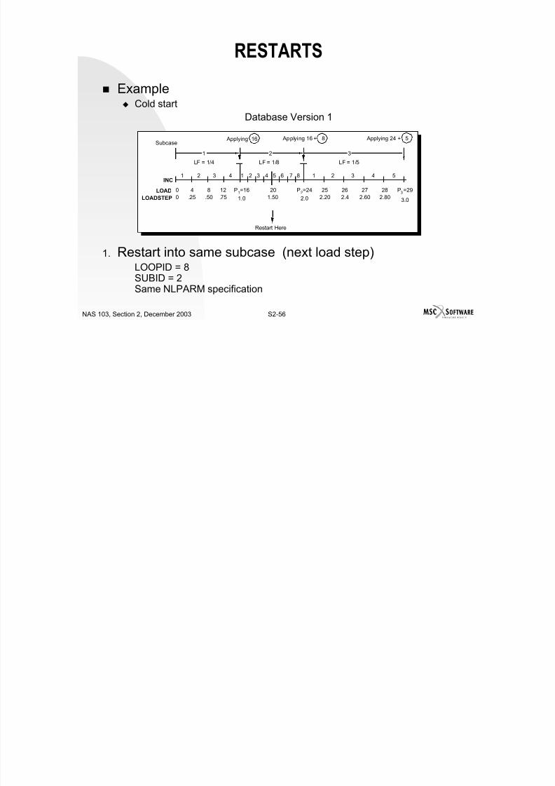
Example Cold start
Database Version 1
1. Restart into same subcase (next load step)LOOPID = 8SUBID = 2Same NLPARM specification
1 2 3 4 5 6 7 81 2 3 4 1 2 3 4 5
00 4.25 8.50 12.75 P1=161.0
201.50 P2=242.0
252.20 262.4 272.60 282.80 P3=293.0
Applying 16
1 2 3
LF = 1/4 LF = 1/8 LF = 1/5
INC
LOADLOADSTEP
Applying 16 + 8 Applying 24 + 5Subcase
Restart Here
RESTARTS

7/21/2019 Nonlinear Analysis Using MSC.nastran
http://slidepdf.com/reader/full/nonlinear-analysis-using-mscnastran 83/783
S2-57NAS 103, Section 2, December 2003
Database Version 2
2. Restart into new subcase before SUBID 3LOOPID = 8SUBID = 3NLPARM specification with 4 increments
INC
LOAD 0 16 20 22 24 29LOADSTEP 0.25 0.50 0.75 1.0 1.5 1.25 1.5 2.0 3.0
LOOPID 4 8 16 21
Restart
RESTARTS

7/21/2019 Nonlinear Analysis Using MSC.nastran
http://slidepdf.com/reader/full/nonlinear-analysis-using-mscnastran 84/783
S2-58NAS 103, Section 2, December 2003
Database Version 3
3. Restart into new subcase after SUBID 3
LOOPID = 8SUBID = 4NLPARM specification with 4 increments
INC
LOAD 0 16 20 22 24 29LOADSTEP 1.0 1.5 2.5 3.0 4.0
LOOPID 4 8 12 17
Restart
RESTARTS

7/21/2019 Nonlinear Analysis Using MSC.nastran
http://slidepdf.com/reader/full/nonlinear-analysis-using-mscnastran 85/783
S2-59NAS 103, Section 2, December 2003
Database Version 4
4. Restart for data recovery
PARAM,LOOPID,n (data recovery for LOOPID 1 through n)
PARAM,SUBID,m (m is the next subcase sequence number)
INC
LOAD 0 16 20 24LOADSTEP 1.0 1.5 3.5 4.0
LOOPID 4 8 12
Restart
RESTARTS

7/21/2019 Nonlinear Analysis Using MSC.nastran
http://slidepdf.com/reader/full/nonlinear-analysis-using-mscnastran 86/783
S2-60NAS 103, Section 2, December 2003
Restarting Into Nonlinear Transient Analysis Requires one parameter
PARAM,SLOOPID,LOOPID
See page 7-67 for more details
Restarting into Normal Mode Solution Sequences Requires one parameter
PARAM,NMLOOP,LOOPID
See page 9-2 for more details
Note: Results may not be accurate if the follower force effects wereincluded in the nonlinear static analysis.
OUTPUT FOR SOLUTION STRATEGIES

7/21/2019 Nonlinear Analysis Using MSC.nastran
http://slidepdf.com/reader/full/nonlinear-analysis-using-mscnastran 87/783
S2-61NAS 103, Section 2, December 2003
Standard Output EUI Normalized error in the displacement.
EPI Normalized error in the load vector.
EWI Normalized error in the energy. LAMBDA Rate of convergence is λi. Solution is diverging if
λi ≥ 1.0., λ1 = 0.1
DLMAG Absolute norm of the load error vector.
FACTOR Scale factor a for line search method.
E-First Initial error E1 before line search begins.
λi
1
2---
E p
i
E pi 1 – ------------- λi 1 –
*
+
= λi
*
min λi .7
λi
10------+ .99,,=
DLMAG R i=
OUTPUT FOR SOLUTION STRATEGIES

7/21/2019 Nonlinear Analysis Using MSC.nastran
http://slidepdf.com/reader/full/nonlinear-analysis-using-mscnastran 88/783
S2-62NAS 103, Section 2, December 2003
E-FINAL Final error Ei after line search terminates.
N-QNV Number of quasi-Newton correction vectors to be used in thecurrent iteration.
N-LS Number of line searches performed. ENIC Expected number of iterations for convergence.
NDV Number of occurrences of probable divergence during theiteration.
MDV Number of occurrences of bisection conditions due to
excessive increments in stress and rotations.
Ni
EPSP E pi
⁄
λi
*
log
-------------------------log=
OUTPUT FOR SOLUTION STRATEGIES
7/21/2019 Nonlinear Analysis Using MSC.nastran
http://slidepdf.com/reader/full/nonlinear-analysis-using-mscnastran 89/783
S2-63NAS 103, Section 2, December 2003
1 SLINE1U: UNSYMMETRIC RIGID PUNCH WITH FRICTION NOVEMBER 30, 1993 MSC/NASTRAN 11/29/93 PAGE 9
00 N O N - L I N E A R I T E R A T I O N M O D U L E O U T P U T STIFFNESS UPDATE TIME .89 SECONDS SUBCASE 1
ITERATION TIME .00 SECONDS LOAD FACTOR .250 - - - CONVERGENCE FACTORS - - - - - - LINE SEARCH DATA - - -0ITERATION EUI EPI EWI LAMBDA DLMAG FACTOR E-FIRST E-FINAL NQNV NLS ENIC NDV MDV 1 9.9000E+01 1.7374E-05 1.7374E-05 1.0000E-01 1.2127E-04 1.0000E+00 3.5268E-07 3.5268E-07 0 0 0 1
2 1.8484E-07 9.0935E-11 7.1947E-17 5.0003E-02 2.6099E-09 1.0000E+00 2.9490E-06 2.9490E-06 0 0 0 0 10*** USER INFORMATION MESSAGE 6186,
*** SOLUTION HAS CONVERGED *** SUBID 1 LOOPID 1 LOAD STEP .250 LOAD FACTOR .25000 ^^^ DMAP INFORMATION MESSAGE 9005 (NLSTATIC) - THE SOLUTION FOR LOOPID= 1 IS SAVED FOR RESTART
SubcaseSequence
Number
For RestartPurpose
OUTPUT FOR SOLUTION STRATEGIES

7/21/2019 Nonlinear Analysis Using MSC.nastran
http://slidepdf.com/reader/full/nonlinear-analysis-using-mscnastran 90/783
S2-64NAS 103, Section 2, December 2003
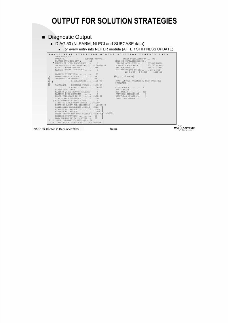
Diagnostic Output DIAG 50 (NLPARM, NLPCI and SUBCASE data)
For every entry into NLITER module (AFTER STIFFNESS UPDATE)
N O N - L I N E A R I T E R A T I O N M O D U L E S O L U T I O N C O N T R O L D A T A LOOP CONTROLS :SUBCASE... 1 SUBCASE RECORD... 1 LARGE DISPLACEMENTS... NONLPARM DATA FOR SET : 110 MACHINE CHARACTERISTICS :NUMBER OF LOAD INCREMENTS ... 1 PRESENT OPEN CORE .... 1607856 WORDSINCREMENTAL TIME INTERVAL ... 0.0000E+00 MODULE’S WORK AREA ... 1601703 WORDSMATRIX UPDATE OPTION ........ ITER MAXIMUM G-SET SIZE ... 160170 TERMSMATRIX UPDATE INCREMENT ..... 1 ESTIMATION FOR NO SPILL ... 22 G-SET +
22 G-SET + 8 A-SET = 1601668MAXIMUM ITERATIONS .......... 25CONVERGENCE OPTIONS ......... PW
INTERMEDIATE OUTPUT ......... YES- DISPLACEMENT ... 1.0E-03 DMAP CONTROL PARAMETERS FROM PREVIOUSITERATION:
TOLERANCE - RESIDUAL FORCE . 1.0E-03- PLASTIC WORK ... 1.0E-07 CONVERGENCE ........ NO
DIVERGENCE LIMIT ............ 3 NEW SUBCASE ........ NOMAXIMUM QUASI-NEWTON VECTORS 0 NEW MATRIX ......... YESMAXIMUM LINE SEARCHES ....... 0 PREVIOUS ITERATIONS 1ERROR TOLERANCE IN YF ....... 2.0E-01 STIFFNESS UPDATES .. 1LINE SEARCH TOLERANCE ....... .500 DMAP LOOP NUMBER ... 1MAX. NUMBER OF BISECTIONS ... 5
LIMIT TO ADJUSTMENT FACTOR .. 20.000ROTATION LIMIT FOR BISECTION .200E+02CONTROLLED INCREMENTS OPTION CRISMINIMUM ARC FACTOR .......... 1.000MAXIMUM ARC FACTOR .......... 1.000SCALE FACTOR FOR LOAD FACTOR 0.000E+00DESIRED ITERATIONS .......... 12MAX. NUMBER OF C. I. STEPS .. 20
0*** USER INFORMATION MESSAGE 6188*** INITIAL ARC LENGTH IS 4.510799D-02
(Approximate)
NLPCI
N L P A R
M
OUTPUT FOR SOLUTION STRATEGIES

7/21/2019 Nonlinear Analysis Using MSC.nastran
http://slidepdf.com/reader/full/nonlinear-analysis-using-mscnastran 91/783
S2-65NAS 103, Section 2, December 2003
DIAG 51 All the data needed to follow the solution process in detail
(displacement, nonlinear force, unbalanced load vector, etc.).
See Section 7.2.5 of the MSC.NASTRAN Handbook for Nonlinear Analysis for details.
Should not be used. It produces enormous output.
Used by developers when debugging.
DIAG 35 Penalty values (gap and friction) for each slave node.
Updated coordinates for slide line nodes.
Detail status for each slide line element (forces, gaps, connectivity, etc.).
RESULT OUTPUT

7/21/2019 Nonlinear Analysis Using MSC.nastran
http://slidepdf.com/reader/full/nonlinear-analysis-using-mscnastran 92/783
S2-66NAS 103, Section 2, December 2003
Results selected for output in the subcase. For example:DISP, FORCE, STRESS, etc. are printed at everyINTOUT load step.
Format:
Example:
Field ContentsINTOUT Intermediate output flag. (Character = “YES”, “NO”, or
“ALL”; Default = NO).
INTOUTNLPARM
10987654321
INTOUT515NLPARM
SOME HEURISTIC OBSERVATIONS

7/21/2019 Nonlinear Analysis Using MSC.nastran
http://slidepdf.com/reader/full/nonlinear-analysis-using-mscnastran 93/783
S2-67NAS 103, Section 2, December 2003
Loose tolerances for convergence test cause difficultiesin later stages.
Sometimes quasi-Newton updates seem to haveadverse effects in creep analysis.
SEMI is a good conservative method if AUTO does notwork. If desperate, use ITER with KSTEP=1 to get
started. A line search is comparable to an iteration in terms of
CPU. However, line searches may be required to getaround some difficulties in convergence.
HINTS AND RECOMMENDATIONS

7/21/2019 Nonlinear Analysis Using MSC.nastran
http://slidepdf.com/reader/full/nonlinear-analysis-using-mscnastran 94/783
S2-68NAS 103, Section 2, December 2003
Identify the type of nonlinearity; if unsure, perform linearanalysis.
Localize nonlinear region; use super-elements and linearelements for the linear region.
Nonlinear region usually needs a finer mesh.
Divide load history by subcases for convenience.
Loads should be subdivided, not to exceed 20 steps ineach subcase.
Select default values to start - NLPARM.
Choose GAP stiffness appropriately. Need to understand the basic theory to use the nonlinear
material.
NLPARM BULK DATA ENTRY

7/21/2019 Nonlinear Analysis Using MSC.nastran
http://slidepdf.com/reader/full/nonlinear-analysis-using-mscnastran 95/783
S2-69NAS 103, Section 2, December 2003
NLPARM with all its field is shown below
Parameters for Nonlinear Static Analysis Control
Defines a set of parameters for nonlinear static analysisiteration strategy.
Format:
Example:
RTOLBMAXRMAXBIS
LSTOLFSTRESSMAXLSMAXQNMAXDIVEPSWEPSPEPSU
INTOUTCONVMAXITERKSTEPKMETHODDTNINCIDNLPARM
10987654321
515NLPARM
SUMMARY
7/21/2019 Nonlinear Analysis Using MSC.nastran
http://slidepdf.com/reader/full/nonlinear-analysis-using-mscnastran 96/783
S2-70NAS 103, Section 2, December 2003
Five tasks in a nonlinear solution strategy Determine an increment to advance forward
Stiffness update
Displacement prediction Element state update
Unbalance force and convergence check
Advancing schemes Constant load increment
Displacement increment
Arc-length increment (Crisfield, Riks, and modified Riks)
SUMMARY

7/21/2019 Nonlinear Analysis Using MSC.nastran
http://slidepdf.com/reader/full/nonlinear-analysis-using-mscnastran 97/783
S2-71NAS 103, Section 2, December 2003
Stiffness update Every iteration (NR method)
Every k-th iteration
Based on the rate of convergence On nonconvergence or divergence
QN updates - Modify the stiffness matrix by two rank one additions
Displacement prediction Solution of equilibrium equations Line Search - Scale the calculated displacements to reduce unbalance
loads
State determination Update element state to calculate element forces
SUMMARY
7/21/2019 Nonlinear Analysis Using MSC.nastran
http://slidepdf.com/reader/full/nonlinear-analysis-using-mscnastran 98/783
S2-72NAS 103, Section 2, December 2003
Convergence criteria Displacement
Load
Energy
Special logics Divergence
Bisection
Time expiration criteria
User interface NLPARM (solution strategy)
SPCD and SPC (displacement increment)
NLPCI (arc-length increment)
WORKSHOP PROBLEMS

7/21/2019 Nonlinear Analysis Using MSC.nastran
http://slidepdf.com/reader/full/nonlinear-analysis-using-mscnastran 99/783
S2-73NAS 103, Section 2, December 2003
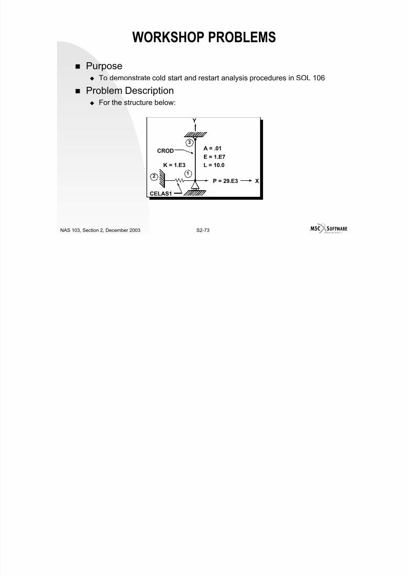
Purpose To demonstrate cold start and restart analysis procedures in SOL 106
Problem Description For the structure below:
Y
P = 29.E3
CROD
CELAS1
K = 1.E3
A = .01
E = 1.E7
L = 10.0
X
3
12
WORKSHOP PROBLEMS
7/21/2019 Nonlinear Analysis Using MSC.nastran
http://slidepdf.com/reader/full/nonlinear-analysis-using-mscnastran 100/783
S2-74NAS 103, Section 2, December 2003
1. Add Case Control commands and Bulk Data entries to:a) Perform geometric nonlinear analysis.
b) Apply a load of 16 × 103 lbs in the first subcase in four increments.
c) Apply a load of 24 × 103 lbs in the second subcase in eight increments.d) Apply a load of 29 × 103 lbs in the third subcase in five increments.
e) For the first subcase, print output at every load step.
f) For the second subcase, use only the work criteria for convergence,
and print output at every load step.g) For the third subcase, request output at the end of the subcase only.
2. Restart the analysis from a load of 20 × 103 lbs. Add anew subcase after the third subcase, and apply in it, a
load of 24 × 103 lbs, using 8 load steps. Also, printoutput at all load steps in this new subcase, and thenext (original subcase 3).
WORKSHOP PROBLEMS 1-2
I t Fil f M difi ti

7/21/2019 Nonlinear Analysis Using MSC.nastran
http://slidepdf.com/reader/full/nonlinear-analysis-using-mscnastran 101/783
S2-75NAS 103, Section 2, December 2003
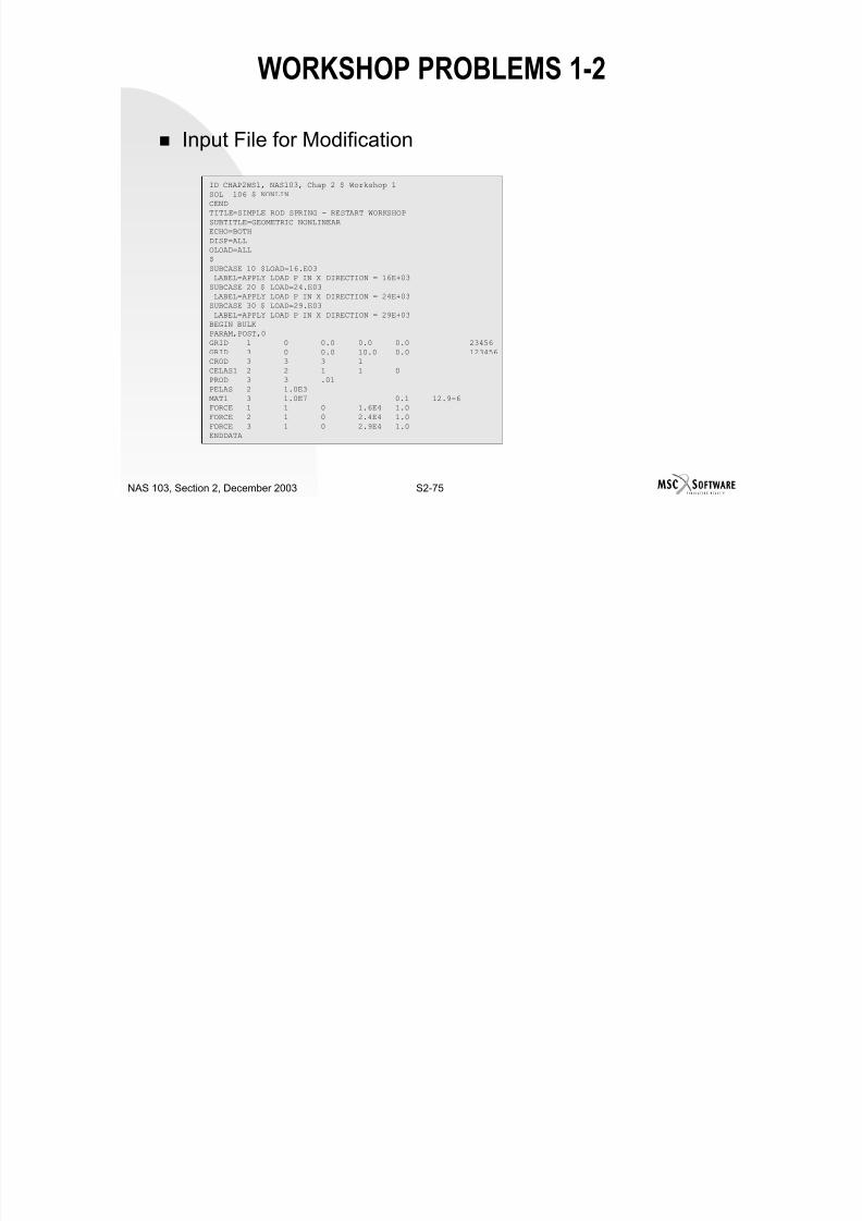
Input File for Modification
ID CHAP2WS1, NAS103, Chap 2 $ Workshop 1
SOL 106 $ NONLINCENDTITLE=SIMPLE ROD SPRING - RESTART WORKSHOP
SUBTITLE=GEOMETRIC NONLINEARECHO=BOTH
DISP=ALLOLOAD=ALL$
SUBCASE 10 $LOAD=16.E03LABEL=APPLY LOAD P IN X DIRECTION = 16E+03
SUBCASE 20 $ LOAD=24.E03LABEL=APPLY LOAD P IN X DIRECTION = 24E+03SUBCASE 30 $ LOAD=29.E03
LABEL=APPLY LOAD P IN X DIRECTION = 29E+03BEGIN BULKPARAM,POST,0GRID 1 0 0.0 0.0 0.0 23456
GRID 3 0 0.0 10.0 0.0 123456CROD 3 3 3 1
CELAS1 2 2 1 1 0PROD 3 3 .01PELAS 2 1.0E3
MAT1 3 1.0E7 0.1 12.9-6FORCE 1 1 0 1.6E4 1.0
FORCE 2 1 0 2.4E4 1.0
FORCE 3 1 0 2.9E4 1.0ENDDATA
SOLUTION FOR WORKSHOP PROBLEM ONE
ID CHAP2WS1s NAS103 Chap 2 $ Workshop 1
7/21/2019 Nonlinear Analysis Using MSC.nastran
http://slidepdf.com/reader/full/nonlinear-analysis-using-mscnastran 102/783
S2-76NAS 103, Section 2, December 2003
BEGIN BULKPARAM,POST,0GRID 1 0 0.0 0.0 0.0 23456GRID 3 0 0.0 10.0 0.0 123456CROD 3 3 3 1CELAS1 2 2 1 1 0PROD 3 3 .01PELAS 2 1.0E3MAT1 3 1.0E7 0.1 12.9-6
FORCE 1 1 0 1.6E4 1.0FORCE 2 1 0 2.4E4 1.0FORCE 3 1 0 2.9E4 1.0PARAM, LGDISP, 1NLPARM, 10, 4, , SEMI, , , , YESNLPARM, 20, 8, , AUTO, , ,W, YESNLPARM, 30, 5, , AUTO, , ,W, NOENDDATA
ID CHAP2WS1s, NAS103, Chap 2 $ Workshop 1SOL 106 $ NONLINCENDTITLE=SIMPLE ROD SPRING - RESTART WORKSHOPSUBTITLE=GEOMETRIC NONLINEARECHO=BOTHDISP=ALLOLOAD=ALL$SUBCASE 10 $LOAD=16.E03
LABEL=APPLY LOAD P IN X DIRECTION = 16E+03LOAD=1NLPARM=10
SUBCASE 20 $ LOAD=24.E03LABEL=APPLY LOAD P IN X DIRECTION = 24E+03LOAD=2NLPARM=20
SUBCASE 30 $ LOAD=29.E03LABEL=APPLY LOAD P IN X DIRECTION = 29E+03LOAD=3NLPARM=30
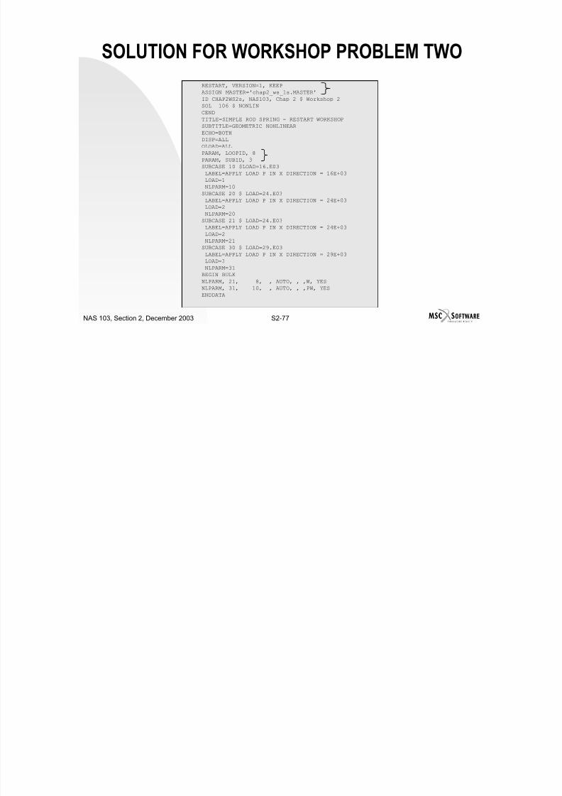
SOLUTION FOR WORKSHOP PROBLEM TWO
RESTART, VERSION=1, KEEP

7/21/2019 Nonlinear Analysis Using MSC.nastran
http://slidepdf.com/reader/full/nonlinear-analysis-using-mscnastran 103/783
S2-77NAS 103, Section 2, December 2003
, ,
ASSIGN MASTER='chap2_ws_1s.MASTER'
ID CHAP2WS2s, NAS103, Chap 2 $ Workshop 2
SOL 106 $ NONLIN
CEND
TITLE=SIMPLE ROD SPRING - RESTART WORKSHOP
SUBTITLE=GEOMETRIC NONLINEAR
ECHO=BOTH
DISP=ALL
OLOAD=ALL
PARAM, LOOPID, 8
PARAM, SUBID, 3
SUBCASE 10 $LOAD=16.E03
LABEL=APPLY LOAD P IN X DIRECTION = 16E+03
LOAD=1
NLPARM=10
SUBCASE 20 $ LOAD=24.E03 LABEL=APPLY LOAD P IN X DIRECTION = 24E+03
LOAD=2
NLPARM=20
SUBCASE 21 $ LOAD=24.E03
LABEL=APPLY LOAD P IN X DIRECTION = 24E+03
LOAD=2
NLPARM=21
SUBCASE 30 $ LOAD=29.E03
LABEL=APPLY LOAD P IN X DIRECTION = 29E+03 LOAD=3
NLPARM=31
BEGIN BULK
NLPARM, 21, 8, , AUTO, , ,W, YES
NLPARM, 31, 10, , AUTO, , ,PW, YES
ENDDATA

7/21/2019 Nonlinear Analysis Using MSC.nastran
http://slidepdf.com/reader/full/nonlinear-analysis-using-mscnastran 104/783
S2-78NAS 103, Section 2, December 2003

7/21/2019 Nonlinear Analysis Using MSC.nastran
http://slidepdf.com/reader/full/nonlinear-analysis-using-mscnastran 105/783
S3-1NAS 103, Section 3, December 2003
SECTION 3
GEOMETRIC NONLINEAR ANALYSIS
7/21/2019 Nonlinear Analysis Using MSC.nastran
http://slidepdf.com/reader/full/nonlinear-analysis-using-mscnastran 106/783
S3-2NAS 103, Section 3, December 2003
TABLE OF CONTENTS
Page

7/21/2019 Nonlinear Analysis Using MSC.nastran
http://slidepdf.com/reader/full/nonlinear-analysis-using-mscnastran 107/783
S3-3NAS 103, Section 3, December 2003
Page
Geometric Nonlinear Analysis 3-4
Simple Geometric Nonlinear Example 3-10
Treatment Of Large Rotations 3-14Follower Forces 3-20
Force1 Bulk Data Entry 3-21
Force2 Bulk Data Entry 3-22
Parameter K6ROT For QUAD4 And TRIA3 3-23
Example Problem One 3-25
Example Problem Two 3-29
Workshop Problem One 3-32
Workshop Problem Two 3-35
Solution For Workshop Problem One 3-37
Solution For Workshop Problem Two 3-40
GEOMETRIC NONLINEAR ANALYSIS
Large displacements and large rotations

7/21/2019 Nonlinear Analysis Using MSC.nastran
http://slidepdf.com/reader/full/nonlinear-analysis-using-mscnastran 108/783
S3-4NAS 103, Section 3, December 2003
Large displacements and large rotations Element deformations are a nonlinear function of the grid point
displacements (nonlinear displacement transformation matrix).
Large displacements Deflection of highly-loaded thin flat plates (geometric stiffening).
where u >> t
t
P
u
GEOMETRIC NONLINEAR ANALYSIS
Large displacements and large rotations (Cont )

7/21/2019 Nonlinear Analysis Using MSC.nastran
http://slidepdf.com/reader/full/nonlinear-analysis-using-mscnastran 109/783
S3-5NAS 103, Section 3, December 2003
Large displacements and large rotations (Cont.) Large rotation.
P
Elastic
GEOMETRIC NONLINEAR ANALYSIS
Follower forces

7/21/2019 Nonlinear Analysis Using MSC.nastran
http://slidepdf.com/reader/full/nonlinear-analysis-using-mscnastran 110/783
S3-6NAS 103, Section 3, December 2003
Follower forces Applied loads are functions of displacements.
Fluid pressure (changes in magnitude and direction).
Tire
GEOMETRIC NONLINEAR ANALYSIS
Follower forces

7/21/2019 Nonlinear Analysis Using MSC.nastran
http://slidepdf.com/reader/full/nonlinear-analysis-using-mscnastran 111/783
S3-7NAS 103, Section 3, December 2003
Follower forces Centrifugal force (proportional to distance from spin axis).
Temperature loads (change in direction).
RFORCE
mr ω2
mr ω2
GEOMETRIC NONLINEAR ANALYSIS
Large strains

7/21/2019 Nonlinear Analysis Using MSC.nastran
http://slidepdf.com/reader/full/nonlinear-analysis-using-mscnastran 112/783
S3-8NAS 103, Section 3, December 2003
g Element strains are nonlinear functions of element deformations.
Rubber Bearing (Hyper elastic Material)
GEOMETRIC NONLINEAR ANALYSIS
User Interface
7/21/2019 Nonlinear Analysis Using MSC.nastran
http://slidepdf.com/reader/full/nonlinear-analysis-using-mscnastran 113/783
S3-9NAS 103, Section 3, December 2003
PARAM LGDISP 0 for no geometric nonlinearity (default).
1 for both nonlinear displacement transformation plus follower forces. 2 for nonlinear displacement transformation only.
Small or large strain depends on the element types.
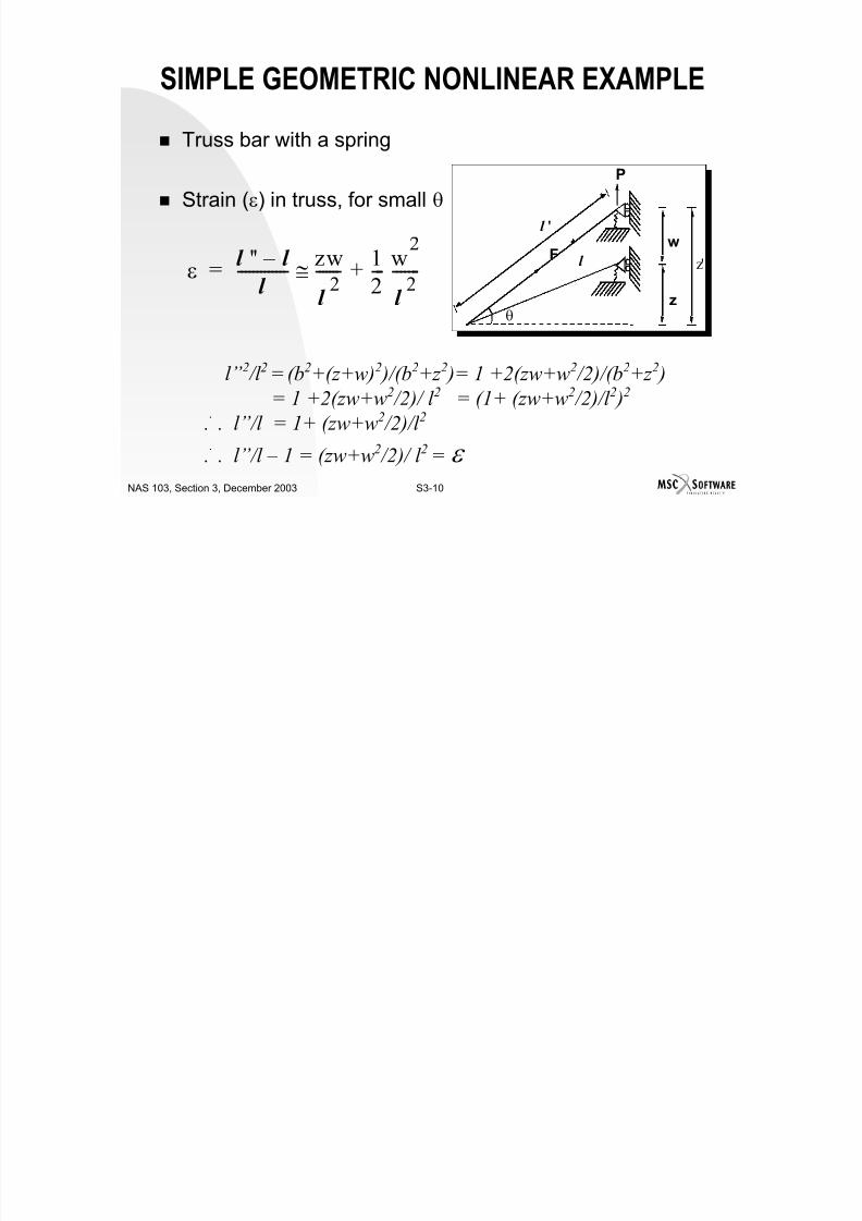
SIMPLE GEOMETRIC NONLINEAR EXAMPLE
Truss bar with a spring
7/21/2019 Nonlinear Analysis Using MSC.nastran
http://slidepdf.com/reader/full/nonlinear-analysis-using-mscnastran 114/783
S3-10NAS 103, Section 3, December 2003
p g
Strain (ε) in truss, for small θ
z
wF
P
l ''
θ
l z'
l”2 /l 2 = (b2+(z+w)2 )/(b2+z 2 )= 1 +2(zw+w2 /2)/(b2+z 2 )
= 1 +2(zw+w2 /2)/ l 2 = (1+ (zw+w2 /2)/l 2 )2
... l”/l = 1+ (zw+w2 /2)/l 2
... l”/l – 1 = (zw+w2 /2)/ l 2 = ε
ε l '' l –
l -------------
zw
l
2-------
1
2---
w
l
2-------+≅=
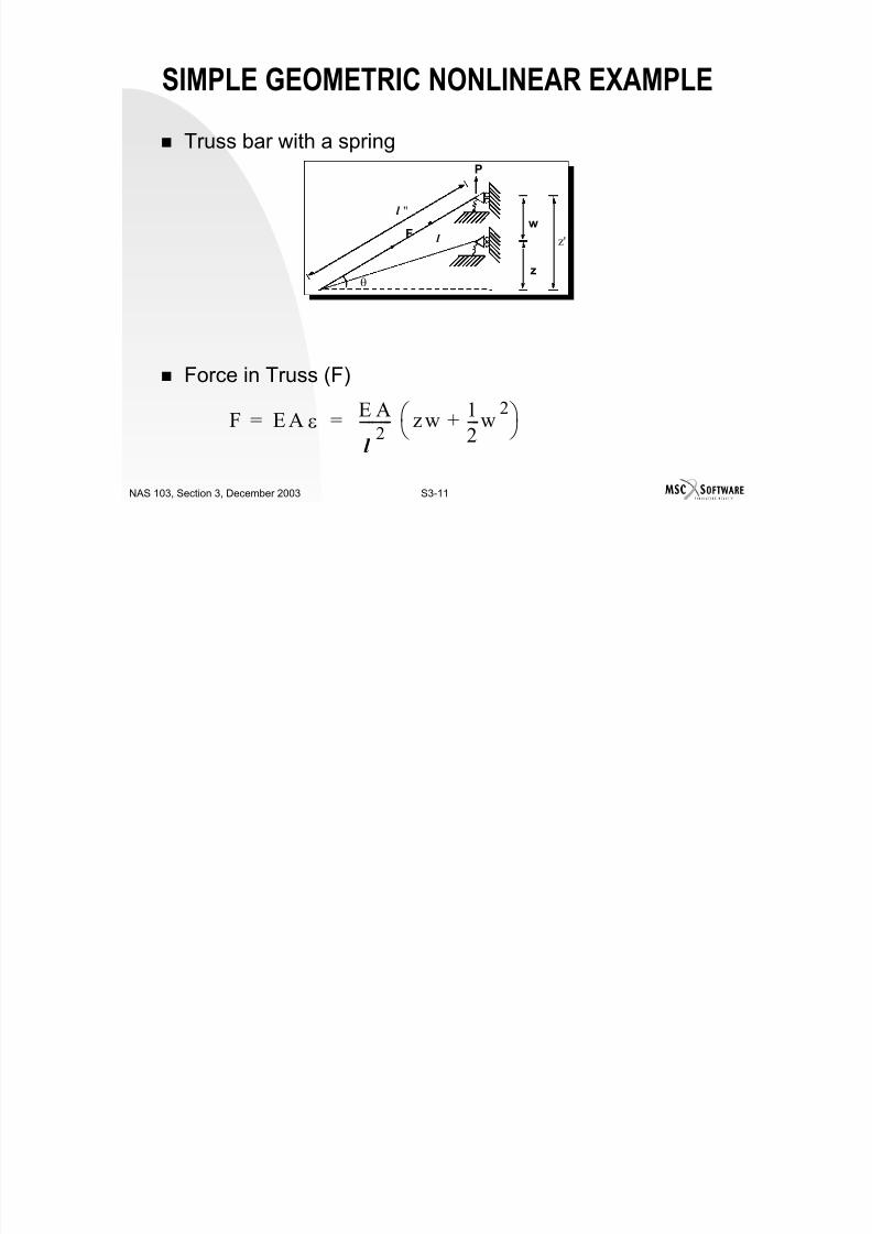
SIMPLE GEOMETRIC NONLINEAR EXAMPLE
Truss bar with a spring
7/21/2019 Nonlinear Analysis Using MSC.nastran
http://slidepdf.com/reader/full/nonlinear-analysis-using-mscnastran 115/783
S3-11NAS 103, Section 3, December 2003
g
Force in Truss (F)
z
wF
P
l ''
θ
l z'
F E A ε=E A
l 2
-------- z w1
2---w
2+
=
SIMPLE GEOMETRIC NONLINEAR EXAMPLE
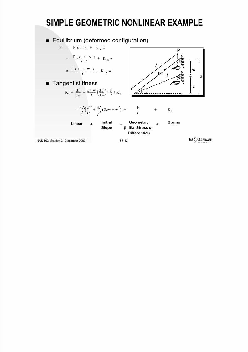
Equilibrium (deformed configuration)
7/21/2019 Nonlinear Analysis Using MSC.nastran
http://slidepdf.com/reader/full/nonlinear-analysis-using-mscnastran 116/783
S3-12NAS 103, Section 3, December 2003
Tangent stiffness
P F θs n K s w+=
F z w+( )
l ' '---------------------= K
s
w+
F z w+( )
l --------------------- K s w+≅
Linear Initial
Slope
Geometric
(Initial Stress or
Differential)
Spring+ + +
K tdP
dw-------
z w+
l -------------
d
d---
F
w----
F
l --- K s+ += =
EA
l --------=
z
l --
2
EA
l
3-------- 2zw w
2+( )
F
l --- K s+ ++
z
wF
P
l ''
θ
l z'
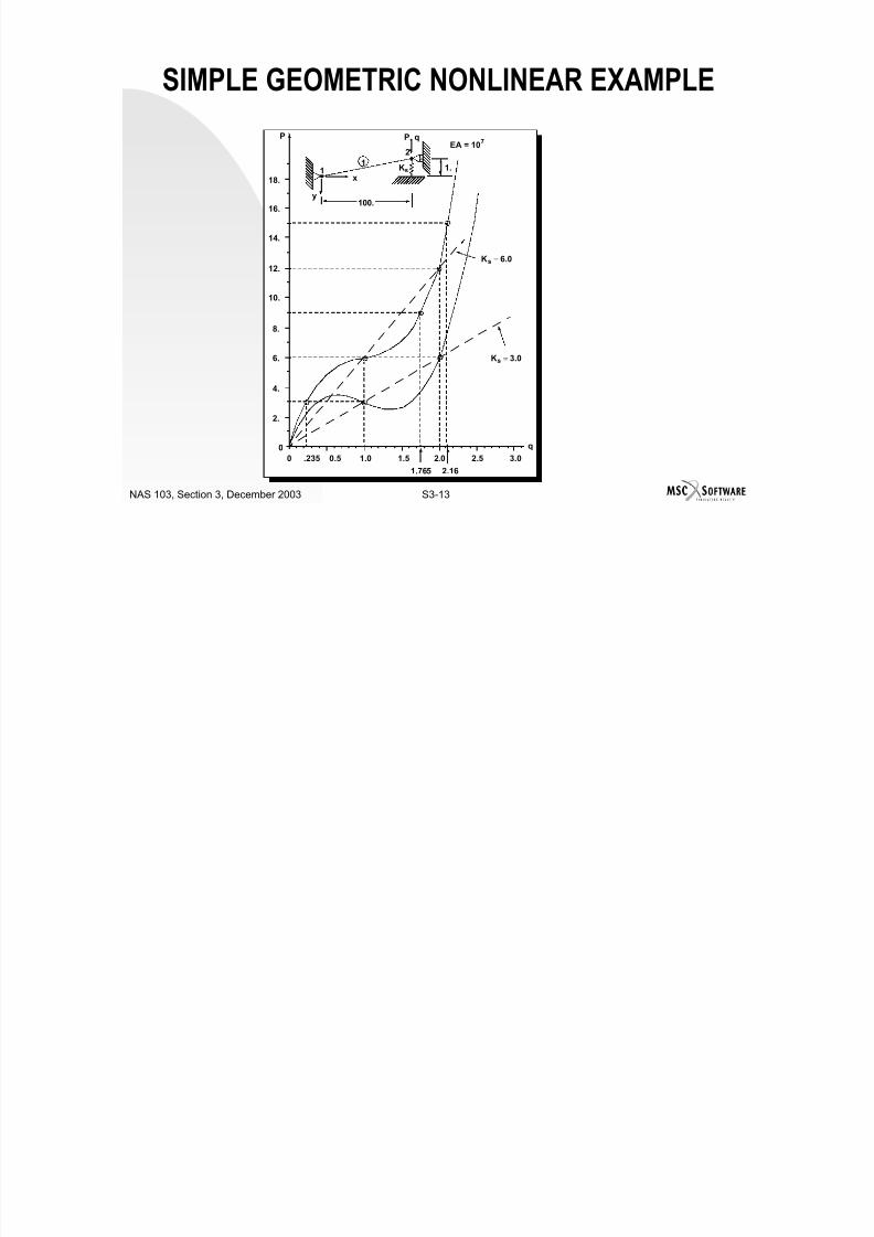
SIMPLE GEOMETRIC NONLINEAR EXAMPLE
P, q
2
PEA = 10
7
7/21/2019 Nonlinear Analysis Using MSC.nastran
http://slidepdf.com/reader/full/nonlinear-analysis-using-mscnastran 117/783
S3-13NAS 103, Section 3, December 2003
11
x
y100.
14.
12.
10.
8.
6.
4.
2.
0
0
0.5 1.0 1.5 2.0 2.5 3.0
q
.235
1.765 2.16
18.
16.
1.Ks
Ks = 6.0
Ks = 3.0
TREATMENT OF LARGE ROTATIONS
Applicable to QUAD4, TRIA3, and BEAM.

7/21/2019 Nonlinear Analysis Using MSC.nastran
http://slidepdf.com/reader/full/nonlinear-analysis-using-mscnastran 118/783
S3-14NAS 103, Section 3, December 2003
Large rotations cannot be added vectorially.
Two approaches: Gimbal angle approach.
Default or selected by PARAM,LANGLE,1.
Rotation vector approach (recommended). Selected by PARAM,LANGLE,2.
User interface PARAM LANGLE.
Specified in Bulk Data Section (cannot specify in the Case ControlSection).
Cannot be changed between subcases or restart.
TREATMENT OF LARGE ROTATIONS
Gimbal Angle Approach - Concept
7/21/2019 Nonlinear Analysis Using MSC.nastran
http://slidepdf.com/reader/full/nonlinear-analysis-using-mscnastran 119/783
S3-15NAS 103, Section 3, December 2003
Rotation matrix is unique.
Several ways to go from one configuration to the other.
Orientation of a rigid body attached to the grid point is obtained by threesuccessive rotations. First, rotation of magnitude θz about the global z-axis.
Second, rotation of magnitude θY about the rotated y-axis.
Third, rotation of magnitude θX about the doubly rotated x-axis.
Note: Above definition produces elegant mathematics, but is difficult tovisualize.
Above definition is equivalent to saying: First, rotation of magnitude θX about the global x-axis.
Second, rotation of magnitude θY about the global y-axis. Third, rotation of magnitude θz about the global z-axis.
Note: With this definition, the mathematics is not elegant.
TREATMENT OF LARGE ROTATIONS
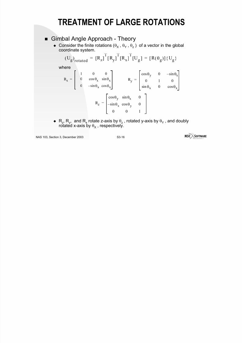
Gimbal Angle Approach - TheoryC id th fi it t ti (θ θ θ ) f t i th l b l

7/21/2019 Nonlinear Analysis Using MSC.nastran
http://slidepdf.com/reader/full/nonlinear-analysis-using-mscnastran 120/783
S3-16NAS 103, Section 3, December 2003
Consider the finite rotations (θX , θY , θz ) of a vector in the globalcoordinate system.
where
Rz, Ry, and Rx rotate z-axis by θz , rotated y-axis by θY , and doublyrotated x-axis by θX , respectively.
Ug( )rotated R z[ ] R y[ ] R x[ ] Ug[ ] R θg( )[ ] Ug = =
R x
1 0 0
0 θxcos θxsin
0 θxsin – θxcos
= R y
θycos 0 θxsin –
0 1 0
θxsin 0 θxcos
=
R z
θycos θxsin 0
θxsin – θycos 0
0 0 1
=
TREATMENT OF LARGE ROTATIONS
For small rotation (δθ)

7/21/2019 Nonlinear Analysis Using MSC.nastran
http://slidepdf.com/reader/full/nonlinear-analysis-using-mscnastran 121/783
S3-17NAS 103, Section 3, December 2003
Addition of gimbal angles
Where (δθ) = incremental rotations in the global system
∆θ = incremental gimbal angle
R δθ( )[ ] R z[ ]T
R y[ ]T
R x[ ]T
1 δθz – δθy
δθz 1 δθx –
δθy – δθx 1
≅=
R θ ∆θ+( )[ ] R δθg
( )[ ] R θg
( )[ ]=
TREATMENT OF LARGE ROTATIONS
Gimbal Angle Incrementsi
7/21/2019 Nonlinear Analysis Using MSC.nastran
http://slidepdf.com/reader/full/nonlinear-analysis-using-mscnastran 122/783
S3-18NAS 103, Section 3, December 2003
Mathematical singularity at θy = 90°.
This condition is usually caused by numerical ill-conditioning.
Use auxiliary angles to avoid singularity. Usual remedy is to use a smaller load increment.
∆θx δθy θz δθx θzcos+sin( ) θycos( )=
∆θy δθy θz δθx – cos θzs n=
∆θz δθz δθz θz δθx θzcos+s n( ) θycos( )[ ] θys n+=
TREATMENT OF LARGE ROTATIONS
Rotation Vector Approach (Version 67 plus)S l t d b PARAM LANGLE 2 i th B lk D t S ti

7/21/2019 Nonlinear Analysis Using MSC.nastran
http://slidepdf.com/reader/full/nonlinear-analysis-using-mscnastran 123/783
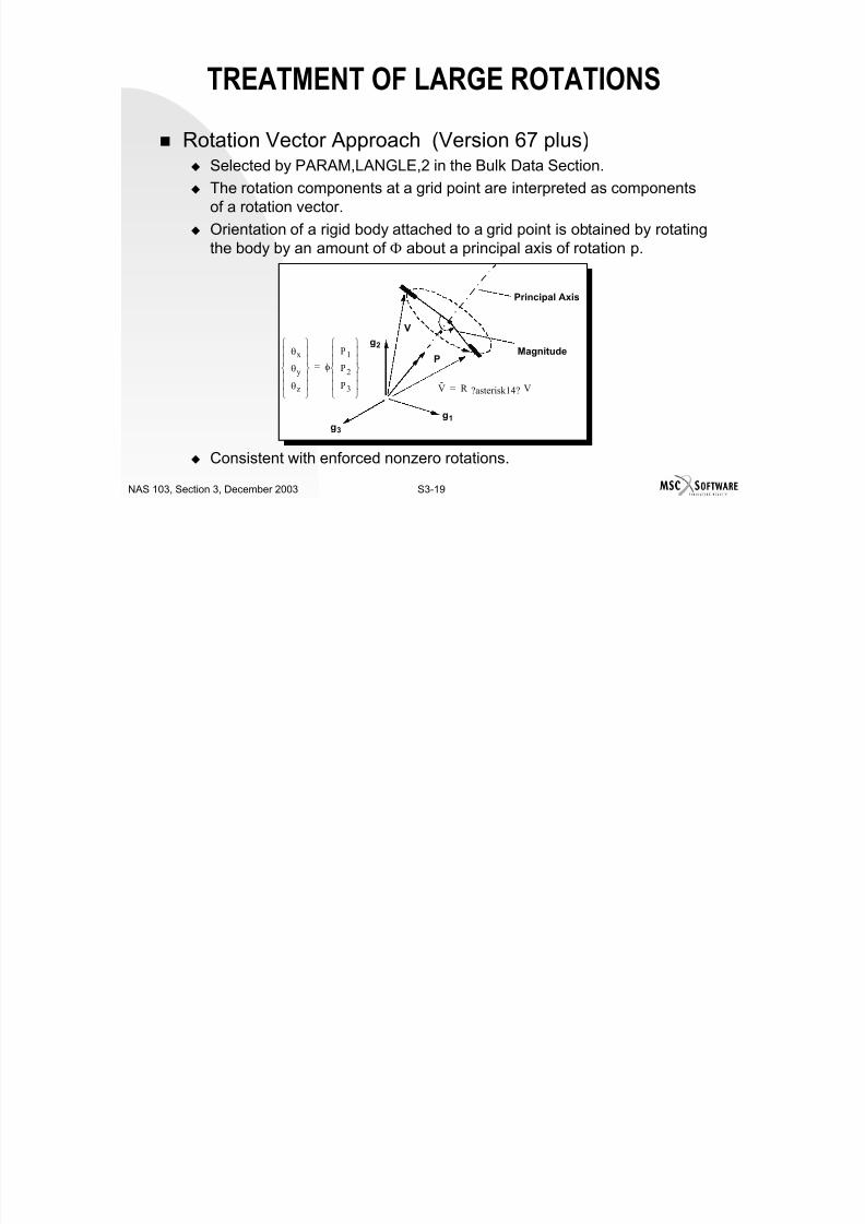
S3-19NAS 103, Section 3, December 2003
Selected by PARAM,LANGLE,2 in the Bulk Data Section.
The rotation components at a grid point are interpreted as components
of a rotation vector. Orientation of a rigid body attached to a grid point is obtained by rotating
the body by an amount of Φ about a principal axis of rotation p.
Consistent with enforced nonzero rotations.
Principal Axis
Magnitude
V
P
g3
g1
g2
V R ?asterisk14? V=
θx
θy
θz
φ
P1
P2
P3
=
FOLLOWER FORCES
Nodal forces change directions with displacements. Load vector(Pa) is a function of the displacement (Ua).

7/21/2019 Nonlinear Analysis Using MSC.nastran
http://slidepdf.com/reader/full/nonlinear-analysis-using-mscnastran 124/783
S3-20NAS 103, Section 3, December 2003
(Pa) is a function of the displacement (Ua).
Must specify PARAM,LGDISP,1.
Applicable to: PLOAD, PLOAD2, and PLOAD4 on QUAD4, TRIA3, HEXA, and PENTA.
PLOADX1 on QUADX and TRIAX hyper elastic elements.
FORCE1, FORCE2, MOMENT1, MOMENT2 (directions dependent upon GRIDlocations).
Temperature load. Centrifugal force.
Corrective loads are computed based on the updated geometry.
Total loads are computed based on the updated geometry.
Note: Tangential stiffness does not include the follower force effect.
FORCE1 BULK DATA ENTRY
FORCE1 Static Force, Alternate Form 1
Defines a static concentrated force by specification of a magnitude

7/21/2019 Nonlinear Analysis Using MSC.nastran
http://slidepdf.com/reader/full/nonlinear-analysis-using-mscnastran 125/783
S3-21NAS 103, Section 3, December 2003
Defines a static concentrated force by specification of a magnitudeand two grid points that determine the direction.
Format:
Example:
Field Contents
SID Load set identification number. (Integer > 0).
G Grid point identification number. (Integer > 0).
F Magnitude of the force. (Real).G1, G2 Grid point identification numbers. (Integer > 0; G1 and G2 may not
be coincident).
G2G1FGSIDFORCE1
10987654321
1316-2.93136FORCE1
FORCE2 BULK DATA ENTRY
FORCE2 Static Force, Alternate Form 2
Defines a static concentrated force by specification of a magnitude
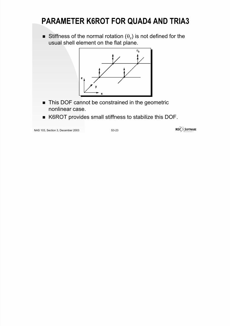
7/21/2019 Nonlinear Analysis Using MSC.nastran
http://slidepdf.com/reader/full/nonlinear-analysis-using-mscnastran 126/783
S3-22NAS 103, Section 3, December 2003
Defines a static concentrated force by specification of a magnitudeand four grid points that determine the direction.
Format:
Example:
Field Contents
SID Load set identification number. (Integer > 0).
G Grid point identification number. (Integer > 0).
F Magnitude of the force. (Real).Gi Grid point identification numbers. (Integer > 0; G1 and G2 may not
be coincident; G3 and G4 cannot be coincident).
G4G3G2G1FGSIDFORCE2
10987654321
13171316-2.93136FORCE2
PARAMETER K6ROT FOR QUAD4 AND TRIA3
Stiffness of the normal rotation (θz) is not defined for theusual shell element on the flat plane.

7/21/2019 Nonlinear Analysis Using MSC.nastran
http://slidepdf.com/reader/full/nonlinear-analysis-using-mscnastran 127/783
S3-23NAS 103, Section 3, December 2003
usua s e e e e o e a p a e
This DOF cannot be constrained in the geometricnonlinear case.
K6ROT provides small stiffness to stabilize this DOF.
y
x
z
θz
PARAMETER K6ROT FOR QUAD4 AND TRIA3
Pseudo stiffness added to the relative rotation in theelement:

7/21/2019 Nonlinear Analysis Using MSC.nastran
http://slidepdf.com/reader/full/nonlinear-analysis-using-mscnastran 128/783
S3-24NAS 103, Section 3, December 2003
element:θz = rotation of a GRID from global displacement
; Rotation Measured in the Element
where G = Shear ModulusS = weighting factor
Pass the constant strain patch test.
No effect on the rigid-body rotation.
Insensitive to the mesh size. Default is K6ROT = 100. which is highly recommended.
Too large a value of K6ROT locks the varying strain by enforcingΩz ≅ θz
−=Ω
y
u
x
v z
δ
δ
δ
δ
2
1
ROT K S t G K z z 6****10)(for 6−=−Ω θ θ
EXAMPLE PROBLEM ONE
Purpose To illustrate geometric nonlinear analysis.
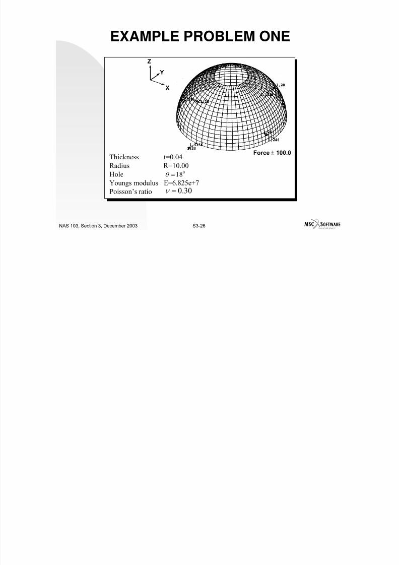
7/21/2019 Nonlinear Analysis Using MSC.nastran
http://slidepdf.com/reader/full/nonlinear-analysis-using-mscnastran 129/783
S3-25NAS 103, Section 3, December 2003
To illustrate geometric nonlinear analysis.
Problem Description Perform large deformation analysis of a hemisphere with a hole at the
top and loaded with four concentrated forces acting on the equator at90° intervals. The perimeter of the hole is constrained in z direction andthe equator is a free edge.
EXAMPLE PROBLEM ONE
Z
Y
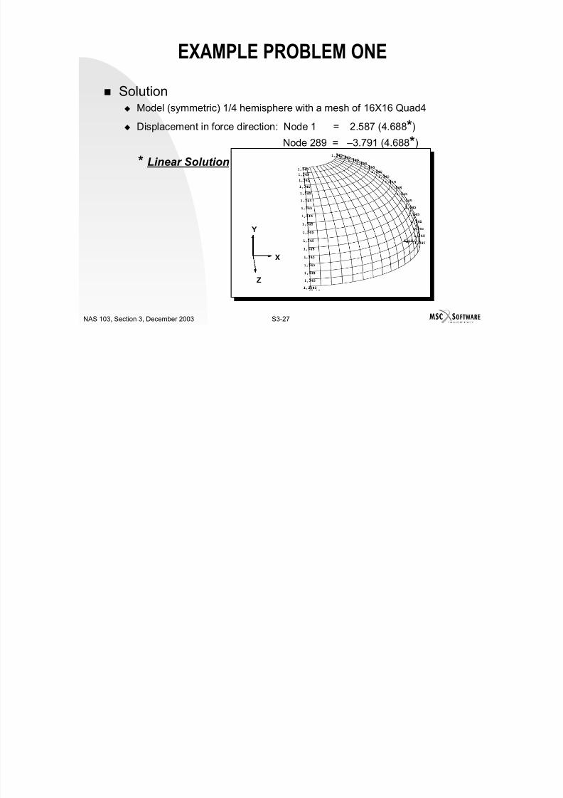
7/21/2019 Nonlinear Analysis Using MSC.nastran
http://slidepdf.com/reader/full/nonlinear-analysis-using-mscnastran 130/783
S3-26NAS 103, Section 3, December 2003
X
Force ± 100.0Thickness t=0.04
Radius R=10.00
Hole
Youngs modulus E=6.825e+7Poisson’s ratio
018=θ
30.0=ν
EXAMPLE PROBLEM ONE
Solution Model (symmetric) 1/4 hemisphere with a mesh of 16X16 Quad4
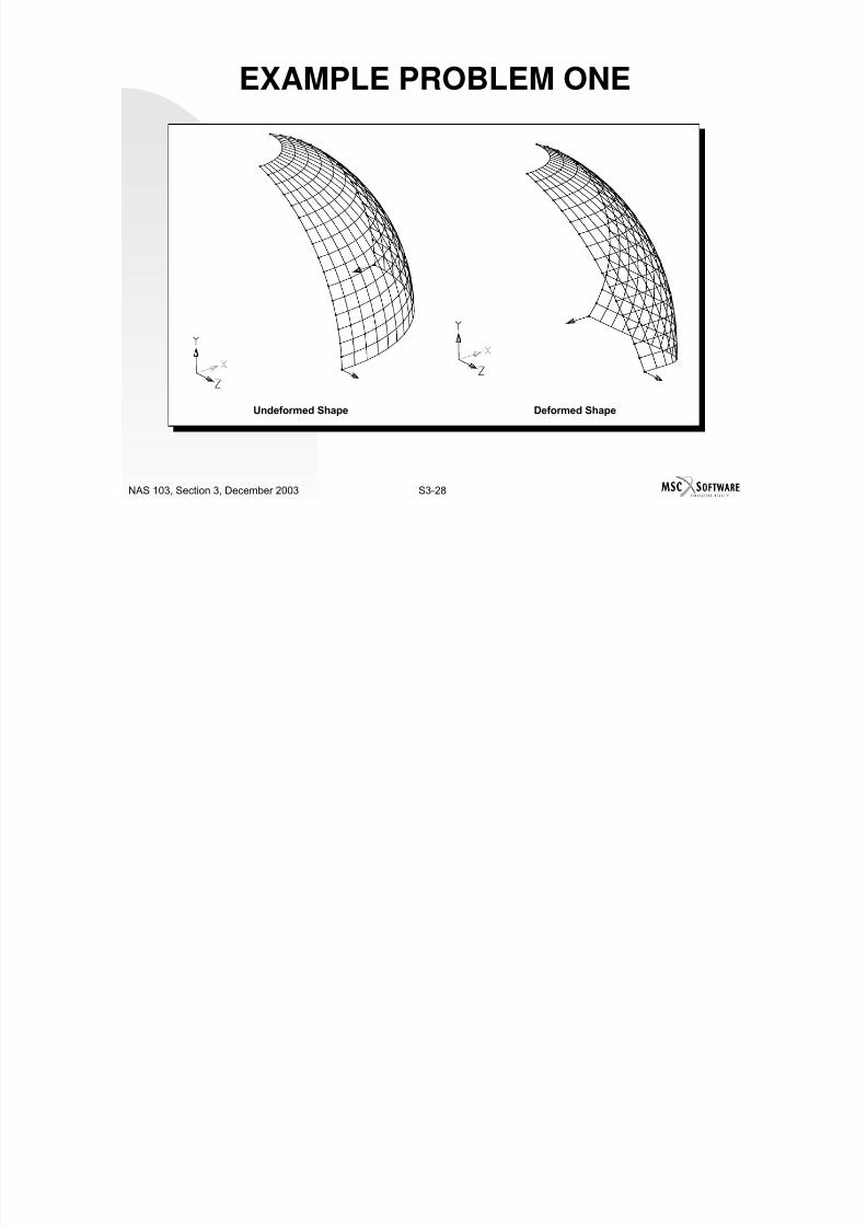
7/21/2019 Nonlinear Analysis Using MSC.nastran
http://slidepdf.com/reader/full/nonlinear-analysis-using-mscnastran 131/783
S3-27NAS 103, Section 3, December 2003
( y ) p
Displacement in force direction: Node 1 = 2.587 (4.688*)
Node 289 = –3.791 (4.688*)
* Linear Solution
Y
X
Z
EXAMPLE PROBLEM ONE

7/21/2019 Nonlinear Analysis Using MSC.nastran
http://slidepdf.com/reader/full/nonlinear-analysis-using-mscnastran 132/783
S3-28NAS 103, Section 3, December 2003
Undeformed Shape Deformed Shape
EXAMPLE PROBLEM TWO
Purpose To illustrate geometric nonlinear analysis.
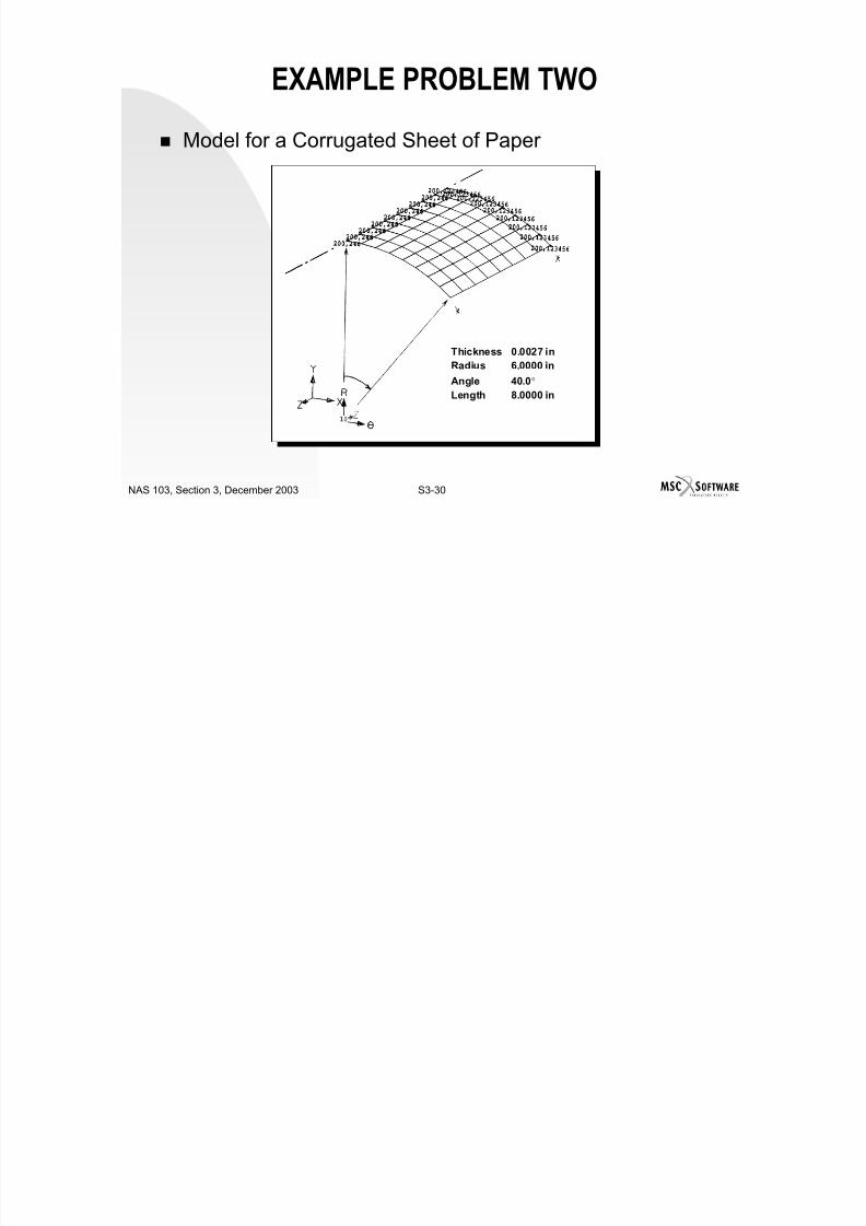
7/21/2019 Nonlinear Analysis Using MSC.nastran
http://slidepdf.com/reader/full/nonlinear-analysis-using-mscnastran 133/783
S3-29NAS 103, Section 3, December 2003
Problem Description Calculate the deformation of a corrugated sheet of paper coming out of
a copy machine. The paper deforms under its own weight.
Solution Perform a quasi-static analysis with a load of 2g to account for dynamic
effects. Model half of the paper taking advantage of symmetry.
EXAMPLE PROBLEM TWO
Model for a Corrugated Sheet of Paper

7/21/2019 Nonlinear Analysis Using MSC.nastran
http://slidepdf.com/reader/full/nonlinear-analysis-using-mscnastran 134/783
S3-30NAS 103, Section 3, December 2003
Thickness 0.0027 in
Radius 6.0000 in
Angle 40.0°Length 8.0000 in
EXAMPLE PROBLEM TWO
Undeformed and Deformed Sheet of Paper for a 2GGravity Load

7/21/2019 Nonlinear Analysis Using MSC.nastran
http://slidepdf.com/reader/full/nonlinear-analysis-using-mscnastran 135/783
S3-31NAS 103, Section 3, December 2003
WORKSHOP PROBLEM ONE
Purpose To demonstrate the use of geometric nonlinear analysis.

7/21/2019 Nonlinear Analysis Using MSC.nastran
http://slidepdf.com/reader/full/nonlinear-analysis-using-mscnastran 136/783
S3-32NAS 103, Section 3, December 2003
Problem Description Calculate the large deflection behavior of the cantilever beam for the
following four load cases:
1. P = 2000.
2. P = 4000.
3. P = 6000.4. P = 8000.
Compare the results with the linear analysis.
WORKSHOP PROBLEM ONE
Properties
y P

7/21/2019 Nonlinear Analysis Using MSC.nastran
http://slidepdf.com/reader/full/nonlinear-analysis-using-mscnastran 137/783
S3-33NAS 103, Section 3, December 2003
L = 10A = 1.
I = 1.e –2
E = 10.e6
y P
x
WORKSHOP PROBLEM ONE
Input File for ModificationBEGIN BULK
$ GEOMETRY
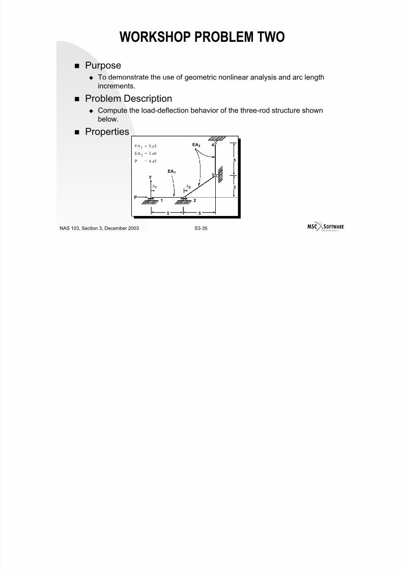
7/21/2019 Nonlinear Analysis Using MSC.nastran
http://slidepdf.com/reader/full/nonlinear-analysis-using-mscnastran 138/783
S3-34NAS 103, Section 3, December 2003
$ GEOMETRY
GRID,1,,0.,0.,0.,,345
=,*(1),=,*(1.),==$
=(9)
GRID,100,,0.,0.,1.,,123456
$ CONNECTIVITY
CBEAM,101,1,1,2,100
=,*(1),=,*(1),*(1),==$
=(8)
$ PROPERTIES
PBEAM,1,1,1.,1.-2,1.-2
MAT1,1,10.E6,,.0
$ CONSTRAINTS
SPC,1,1,123456
$ LOADING
FORCE,11,11,,1.E4,0.,1.,0.
LOAD,200,.2,1.,11
LOAD,400,.4,1.,11
LOAD,600,.6,1.,11
LOAD,800,.8,1.,11
$ PARAMETERS
PARAM,POST,0
$ SOLUTION STRATEGY
ENDDATA
ID CHAP3W1, NAS103W $ AR (12/03)
SOL 106
TIME 10
CEND
TITLE=TRACE LARGE DEFLECTION OF A CANTILEVERED BEAM
SUBTITLE=Ref: BISSHOPP & DRUCKER; QAM 3(1):272-275; 1945SPC=1
DISP=ALL
SPCF=ALL
$
SUBCASE 10
LOAD=200
$
SUBCASE 20
LOAD=400
$
SUBCASE 30
LOAD=600
$
SUBCASE 40
LOAD=800
WORKSHOP PROBLEM TWO
Purpose To demonstrate the use of geometric nonlinear analysis and arc length
increments

7/21/2019 Nonlinear Analysis Using MSC.nastran
http://slidepdf.com/reader/full/nonlinear-analysis-using-mscnastran 139/783
S3-35NAS 103, Section 3, December 2003
increments.
Problem Description Compute the load-deflection behavior of the three-rod structure shown
below.
Properties
3
21P
5 5
5
3
4
y
EA1 5.e5=
EA2 3.e6=
P 4.e5=
EA2
EA1
∆2
∆1
WORKSHOP PROBLEM TWO
Input File for ModificationID CHAP32W2, NAS103 Workshop 2 $ AR (12/03)SOL 106CEND

7/21/2019 Nonlinear Analysis Using MSC.nastran
http://slidepdf.com/reader/full/nonlinear-analysis-using-mscnastran 140/783
S3-36NAS 103, Section 3, December 2003
TITLE=GEOMETRIC NONLINEAR PROBLEMSUBTITLE=Ref: POWELL & SIMONS, IJNME, 17:1455-1467, 1981SPCF=ALL
SPC=12LOAD=10SUBCASE 10BEGIN BULK$ GEMOETRYGRID,1,,0.0,0.GRID,2,,5.,0.GRID,3,,10.,3.GRID,4,,10.,8.GRDSET,,,,,,,3456$ CONNECTIVITYCONROD,1,1,2,10,.5CONROD,2,2,3,11,1.CONROD,3,3,4,11,1.$ PROPERTIESMAT1,10,1.E6MAT1,11,3.E6$ CONSTRAINTSSPC1,12,1,3SPC1,12,2,1,2SPC1,12,12,4
$ LOADINGFORCE,10,1,,4.E5,1.,0.,0.$ PARAMETERSPARAM,POST,0$ SOLUTION STRATEGYENDDATA
SOLUTION FOR WORKSHOP PROBLEM ONE
ID CHAP3W1S, NAS103W $ AR (12/03)
SOL 106
TIME 10
CEND
TITLE=TRACE LARGE DEFLECTION OF A CANTILEVERED BEAM
SUBTITLE=Ref: BISSHOPP & DRUCKER; QAM 3(1):272-275; 1945
BEGIN BULK
$ GEOMETRY
GRID,1,,0.,0.,0.,,345
=,*(1),=,*(1.),==$
=(9)
GRID 100 0 0 1 123456
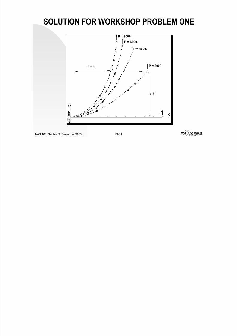
7/21/2019 Nonlinear Analysis Using MSC.nastran
http://slidepdf.com/reader/full/nonlinear-analysis-using-mscnastran 141/783
S3-37NAS 103, Section 3, December 2003
SUBTITLE Ref: BISSHOPP & DRUCKER; QAM 3(1):272 275; 1945
SPC=1
DISP=ALL
SPCF=ALLNLPARM=10
$
SUBCASE 10
LOAD=200
$
SUBCASE 20
LOAD=400
$
SUBCASE 30LOAD=600
$
SUBCASE 40
LOAD=800
GRID,100,,0.,0.,1.,,123456
$ CONNECTIVITY
CBEAM,101,1,1,2,100
=,*(1),=,*(1),*(1),==$=(8)
$ PROPERTIES
PBEAM,1,1,1.,1.-2,1.-2
MAT1,1,10.E6,,.0
$ CONSTRAINTS
SPC,1,1,123456
$ LOADING
FORCE,11,11,,1.E4,0.,1.,0.
LOAD,200,.2,1.,11LOAD,400,.4,1.,11
LOAD,600,.6,1.,11
LOAD,800,.8,1.,11
$ PARAMETERS
PARAM,POST,0
$ SOLUTION STRATEGY
NLPARM,10,10
PARAM,LGDISP,1
ENDDATA
SOLUTION FOR WORKSHOP PROBLEM ONE
P = 8000.
P = 6000.
P = 4000.
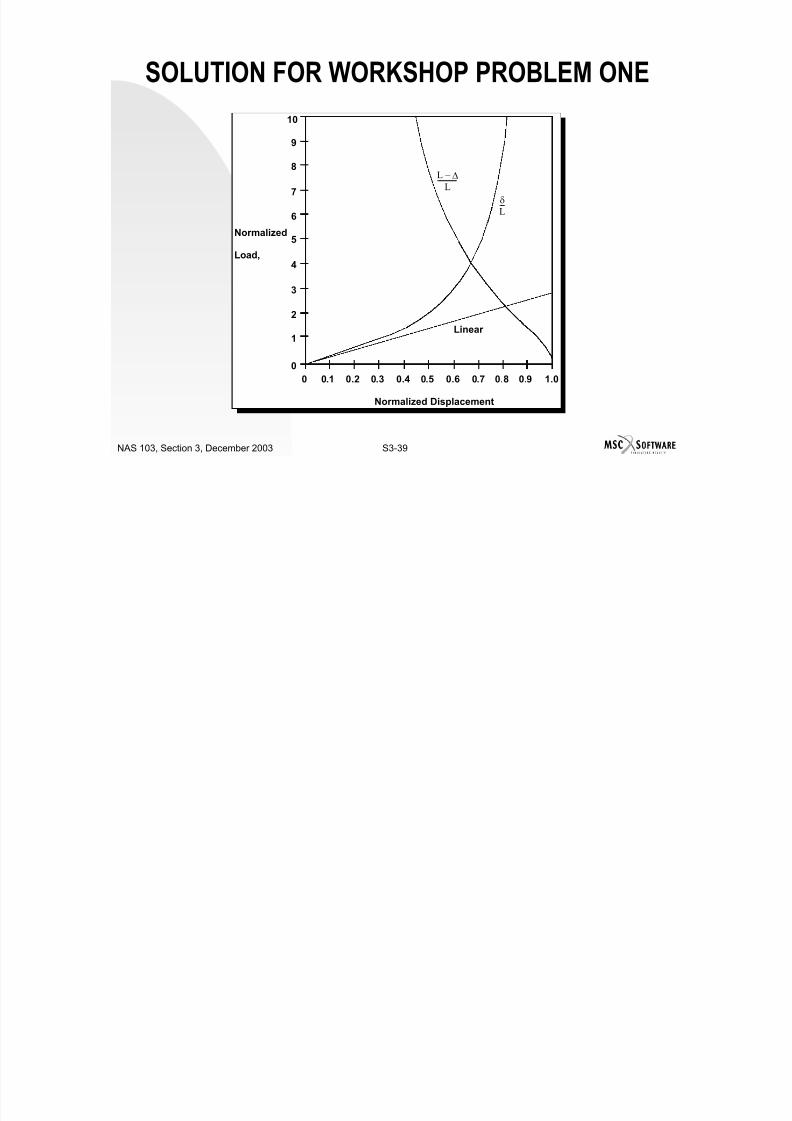
7/21/2019 Nonlinear Analysis Using MSC.nastran
http://slidepdf.com/reader/full/nonlinear-analysis-using-mscnastran 142/783
S3-38NAS 103, Section 3, December 2003
P = 2000.
PX
Y
L – ∆
δ
8
9
10
L ∆
SOLUTION FOR WORKSHOP PROBLEM ONE

7/21/2019 Nonlinear Analysis Using MSC.nastran
http://slidepdf.com/reader/full/nonlinear-analysis-using-mscnastran 143/783
S3-39NAS 103, Section 3, December 2003
00 0.1 0.2 0.3 0.4 0.5 0.6 0.7 0.8 0.9 1.0
1
2
3
4
5
6
7
Linear
Normalized Displacement
Normalized
Load,
L ∆ –
L-------------
δL---
$ CONNECTIVITY
CONROD,1,1,2,10,.5
CONROD,2,2,3,11,1.
CONROD,3,3,4,11,1.
$ PROPERTIES
MAT1 10 1 E6
ID CHAP32W2S, NAS103 Workshop 2 $ AR (12/03)
SOL 106
CEND
TITLE=GEOMETRIC NONLINEAR PROBLEM
SUBTITLE=Ref: POWELL & SIMONS, IJNME, 17:1455-1467, 1981
SPCF=ALL
SOLUTION FOR WORKSHOP PROBLEM TWO
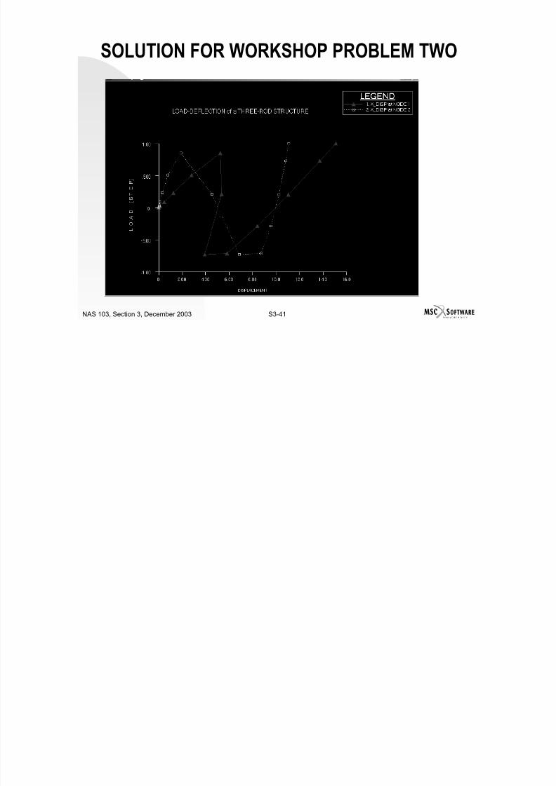
7/21/2019 Nonlinear Analysis Using MSC.nastran
http://slidepdf.com/reader/full/nonlinear-analysis-using-mscnastran 144/783
S3-40NAS 103, Section 3, December 2003
MAT1,10,1.E6
MAT1,11,3.E6
$ CONSTRAINTS
SPC1,12,1,3SPC1,12,2,1,2
SPC1,12,12,4
$ LOADING
FORCE,10,1,,4.E5,1.,0.,0.
$ PARAMETERS
PARAM,POST,0
$ SOLUTION STRATEGY
NLPARM,10,40,,,,,,YES
NLPCI,10PARAM,LGDISP,1
ENDDATA
SPC=12
LOAD=10
SUBCASE 10NLPARM=10
BEGIN BULK
$ GEMOETRY
GRID,1,,0.0,0.
GRID,2,,5.,0.
GRID,3,,10.,3.
GRID,4,,10.,8.
GRDSET,,,,,,,3456
SOLUTION FOR WORKSHOP PROBLEM TWO

7/21/2019 Nonlinear Analysis Using MSC.nastran
http://slidepdf.com/reader/full/nonlinear-analysis-using-mscnastran 145/783
S3-41NAS 103, Section 3, December 2003

7/21/2019 Nonlinear Analysis Using MSC.nastran
http://slidepdf.com/reader/full/nonlinear-analysis-using-mscnastran 146/783
S3-42NAS 103, Section 3, December 2003

7/21/2019 Nonlinear Analysis Using MSC.nastran
http://slidepdf.com/reader/full/nonlinear-analysis-using-mscnastran 147/783
S4-1NAS 103, Section 4, December 2003
SECTION 4
NONLINEAR BUCKLING ANALYSIS

7/21/2019 Nonlinear Analysis Using MSC.nastran
http://slidepdf.com/reader/full/nonlinear-analysis-using-mscnastran 148/783
S4-2NAS 103, Section 4, December 2003
TABLE OF CONTENTS
Page
Instability Phenomena 4-4
Linear Versus Nonlinear Buckling 4-7
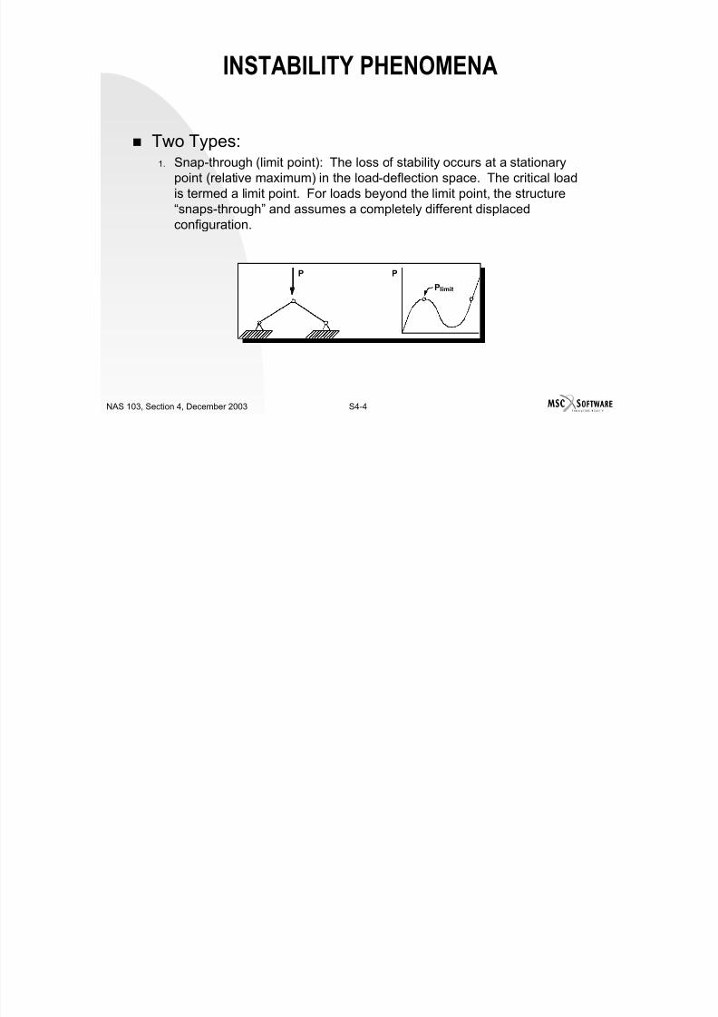
7/21/2019 Nonlinear Analysis Using MSC.nastran
http://slidepdf.com/reader/full/nonlinear-analysis-using-mscnastran 149/783
S4-3NAS 103, Section 4, December 2003
Nonlinear Buckling Analysis 4-9
Example Problem One 4-15Example Problem Two 4-20
Workshop Problems 4-29
Solution For Workshop Problem One 4-32
Solution For Workshop Problem Two 4-34Solution For Workshop Problem Three 4-35
Solution For Workshop Problem Four 4-37
INSTABILITY PHENOMENA
Two Types:1 Snap-through (limit point): The loss of stability occurs at a stationary

7/21/2019 Nonlinear Analysis Using MSC.nastran
http://slidepdf.com/reader/full/nonlinear-analysis-using-mscnastran 150/783
S4-4NAS 103, Section 4, December 2003
1. Snap through (limit point): The loss of stability occurs at a stationary
point (relative maximum) in the load-deflection space. The critical loadis termed a limit point. For loads beyond the limit point, the structure“snaps-through” and assumes a completely different displacedconfiguration.
P P
Plimit
INSTABILITY PHENOMENA
Snap-Through of Shallow Shells
P

7/21/2019 Nonlinear Analysis Using MSC.nastran
http://slidepdf.com/reader/full/nonlinear-analysis-using-mscnastran 151/783
S4-5NAS 103, Section 4, December 2003
Shallow arch is symmetric; Deep arch is anti-symmetric.
Question of stable and unstable path.
Arc-length increments are good for snap-through problems.
INSTABILITY PHENOMENA
2. Bifurcation buckling: The loss of stability occurs when two or moreequilibrium paths intersect in the load-deflection space. The point ofintersection is termed a bifurcation point. For loads beyond thebifurcation point, the structure buckles.
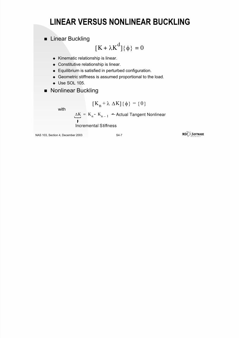
7/21/2019 Nonlinear Analysis Using MSC.nastran
http://slidepdf.com/reader/full/nonlinear-analysis-using-mscnastran 152/783
S4-6NAS 103, Section 4, December 2003
p
Arc length increments may not pick a bifurcation buckling point.
P
Pcrit
P
∆
LINEAR VERSUS NONLINEAR BUCKLING
Linear Buckling
K λKd
+[ ] φ 0=

7/21/2019 Nonlinear Analysis Using MSC.nastran
http://slidepdf.com/reader/full/nonlinear-analysis-using-mscnastran 153/783
S4-7NAS 103, Section 4, December 2003
Kinematic relationship is linear.
Constitutive relationship is linear.
Equilibrium is satisfied in perturbed configuration.
Geometric stiffness is assumed proportional to the load.
Use SOL 105.
Nonlinear Buckling
withK n λ ∆K +[ ] φ 0 =
Incremental Stiffness
Actual Tangent Nonlinear∆K Kn
Kn 1–
= -
LINEAR VERSUS NONLINEAR BUCKLING
Kinematic relationship is nonlinear.
Constitutive relationship may be nonlinear.

7/21/2019 Nonlinear Analysis Using MSC.nastran
http://slidepdf.com/reader/full/nonlinear-analysis-using-mscnastran 154/783
S4-8NAS 103, Section 4, December 2003
Geometric stiffness is assumed proportional to displacement increment.
Equilibrium is satisfied in perturbed configuration.
Use SOL 106.
NONLINEAR BUCKLING ANALYSIS
Two ways to predict the limit load: Arc length increments to trace the equilibrium path.
(may be expensive, and requires some idea of the limit load.)
PARAM BUCKLE th d

7/21/2019 Nonlinear Analysis Using MSC.nastran
http://slidepdf.com/reader/full/nonlinear-analysis-using-mscnastran 155/783
S4-9NAS 103, Section 4, December 2003
PARAM,BUCKLE method.
One way to predict bifurcation buckling: PARAM,BUCKLE method.
NONLINEAR BUCKLING ANALYSIS
PARAM,BUCKLE Concept
Limit Point or
Bifurcation ∆ K
P
K
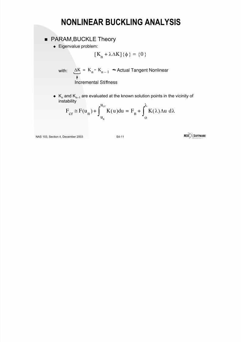
7/21/2019 Nonlinear Analysis Using MSC.nastran
http://slidepdf.com/reader/full/nonlinear-analysis-using-mscnastran 156/783
S4-10NAS 103, Section 4, December 2003
Note:The error in Ucr
may be large, but the corresponding error in Pcr
issmall.
Bifurcation
∆U
λ∆U
Un – 1 Un UUcr
Pcr
Pn
Pn – 1
α∆P∆P
Predicted by Analysis
UUn – 1 Un Ucr U'cr
NONLINEAR BUCKLING ANALYSIS
PARAM,BUCKLE Theory Eigenvalue problem:
Kn
λ∆K+[ ] φ 0 =
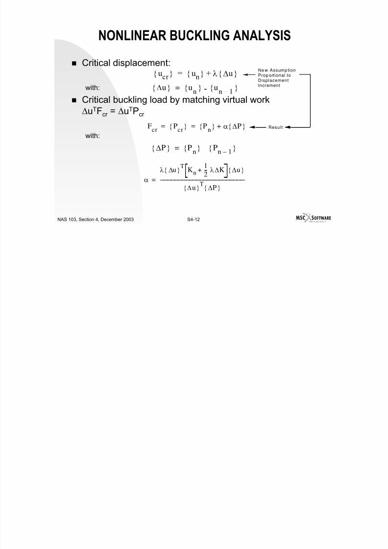
7/21/2019 Nonlinear Analysis Using MSC.nastran
http://slidepdf.com/reader/full/nonlinear-analysis-using-mscnastran 157/783
S4-11NAS 103, Section 4, December 2003
with:
Kn and Kn–1 are evaluated at the known solution points in the vicinity ofinstability
n
Fcr
F un
( ) K u( ) udun
ucr
∫F
nK
o
λ
∫ λ( )∆u dλ+=+≅
Incremental Stiffness
Actual Tangent Nonlinear∆K Kn
Kn 1–
= -
NONLINEAR BUCKLING ANALYSIS
Critical displacement:
with:
Ne w Assump tionProp ortional toDisplacementIncrement
ucr un λ ∆u +=
∆u un
un 1–
= -
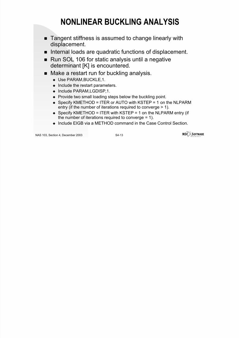
7/21/2019 Nonlinear Analysis Using MSC.nastran
http://slidepdf.com/reader/full/nonlinear-analysis-using-mscnastran 158/783
S4-12NAS 103, Section 4, December 2003
Critical buckling load by matching virtual work∆uTFcr = ∆uTPcr
with:ResultF
crP
cr P
n α ∆P += =
∆P Pn
Pn 1–
=
α
λ ∆u T
Kn1
2--- λ∆K+ ∆u
∆u T ∆P ----------------------------------------------------------------------=
n n 1
NONLINEAR BUCKLING ANALYSIS
Tangent stiffness is assumed to change linearly withdisplacement.
Internal loads are quadratic functions of displacement.

7/21/2019 Nonlinear Analysis Using MSC.nastran
http://slidepdf.com/reader/full/nonlinear-analysis-using-mscnastran 159/783
S4-13NAS 103, Section 4, December 2003
Run SOL 106 for static analysis until a negativedeterminant [K] is encountered. Make a restart run for buckling analysis.
Use PARAM,BUCKLE,1.
Include the restart parameters. Include PARAM,LGDISP,1. Provide two small loading steps below the buckling point. Specify KMETHOD = ITER or AUTO with KSTEP = 1 on the NLPARM
entry (if the number of iterations required to converge > 1).
Specify KMETHOD = ITER with KSTEP = 1 on the NLPARM entry (ifthe number of iterations required to converge = 1). Include EIGB via a METHOD command in the Case Control Section.
NONLINEAR BUCKLING ANALYSIS
Make a restart run for buckling analysis. (Cont.) Provide mode shape PLOT commands if desired.
Sometimes, a negative determinant of [K] may be encountered due tonumerical reasons.
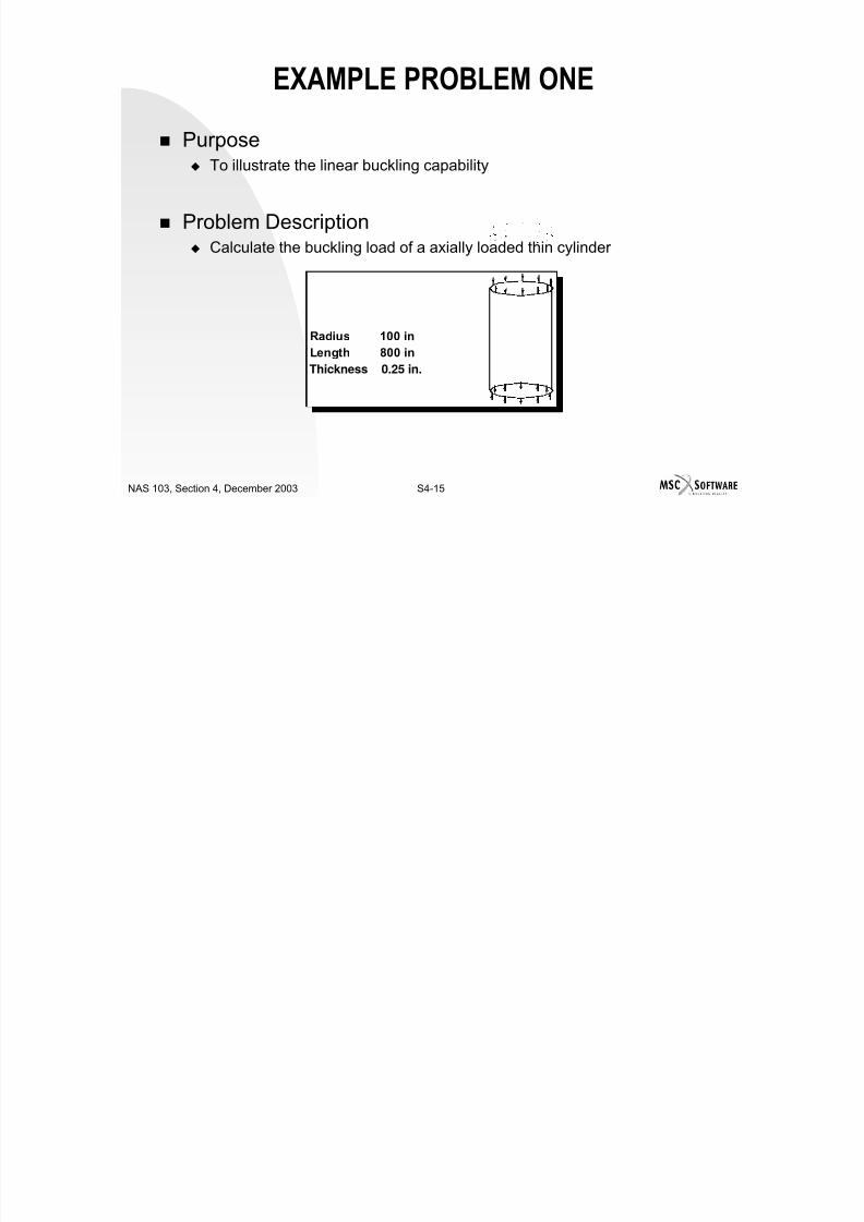
7/21/2019 Nonlinear Analysis Using MSC.nastran
http://slidepdf.com/reader/full/nonlinear-analysis-using-mscnastran 160/783
S4-14NAS 103, Section 4, December 2003
numerical reasons.
A good idea may be to perform at least two buckling analyses withdifferent restarting points and compare the calculated buckling (limit)load.
Look for sudden increase in displacement values to make sure that the
load is in the vicinity of a limit point.
EXAMPLE PROBLEM ONE
Purpose To illustrate the linear buckling capability

7/21/2019 Nonlinear Analysis Using MSC.nastran
http://slidepdf.com/reader/full/nonlinear-analysis-using-mscnastran 161/783
S4-15NAS 103, Section 4, December 2003
Problem Description Calculate the buckling load of a axially loaded thin cylinder
Radius 100 in
Length 800 in
Thickness 0.25 in.
EXAMPLE PROBLEM ONE
Solution Use SOL 105.
Only one half of the cylinder is modeled due to symmetry.
64 QUAD4 elements in the circumferential direction and 40 QUAD4

7/21/2019 Nonlinear Analysis Using MSC.nastran
http://slidepdf.com/reader/full/nonlinear-analysis-using-mscnastran 162/783
S4-16NAS 103, Section 4, December 2003
64 QUAD4 elements in the circumferential direction and 40 QUAD4
elements in the longitudinal direction.
Note:1. Could use cyclic symmetry to get buckling load.
2. Cannot plot buckling shape using cyclic symmetry for the full model.
EXAMPLE PROBLEM ONE
Model
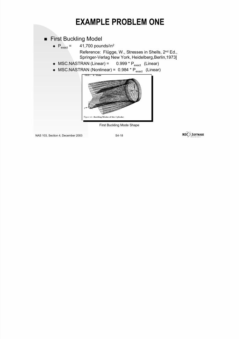
7/21/2019 Nonlinear Analysis Using MSC.nastran
http://slidepdf.com/reader/full/nonlinear-analysis-using-mscnastran 163/783
S4-17NAS 103, Section 4, December 2003
EXAMPLE PROBLEM ONE
First Buckling Model Pexact = 41,700 pounds/in2
Reference: Flügge, W., Stresses in Shells, 2nd Ed.,Springer-Verlag New York, Heidelberg,Berlin,1973]
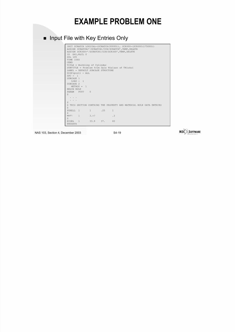
7/21/2019 Nonlinear Analysis Using MSC.nastran
http://slidepdf.com/reader/full/nonlinear-analysis-using-mscnastran 164/783
S4-18NAS 103, Section 4, December 2003
MSC.NASTRAN (Linear) = 0.999 * Pexact (Linear) MSC.NASTRAN (Nonlinear) = 0.984 * Pexact (Linear)
First Buckling Mode Shape
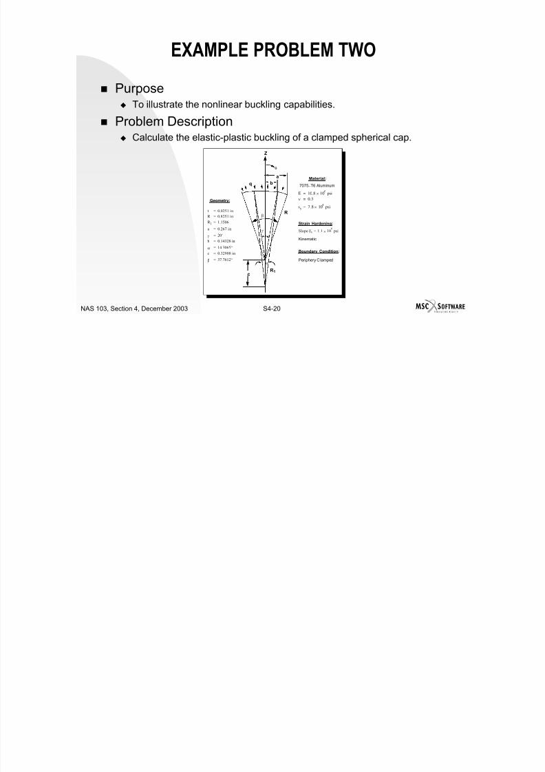
7/21/2019 Nonlinear Analysis Using MSC.nastran
http://slidepdf.com/reader/full/nonlinear-analysis-using-mscnastran 165/783
EXAMPLE PROBLEM TWO
Purpose To illustrate the nonlinear buckling capabilities.
Problem Description

7/21/2019 Nonlinear Analysis Using MSC.nastran
http://slidepdf.com/reader/full/nonlinear-analysis-using-mscnastran 166/783
S4-20NAS 103, Section 4, December 2003
Calculate the elastic-plastic buckling of a clamped spherical cap.
q
cR1
b
a
R
Geometry:
t 0.0251 in=
R 0.8251 in=
R 1 1.1506=
a 0.267 in=
γ 20o=
b 0.14328 in=
α 14.3065 o=
c 0.32908 in=
β 37.7612 o=
Z
Slope Et 1.1 106 psi×=
Kinematic
Strain Hardening:
Boundary Condition:
Periphery Clamped
Material:
7075 – T6 Aluminum
γ
α
β
θ
E 10.8 106 psi×=
ν 0.3=
sy 7.8 104 psi×=
EXAMPLE PROBLEM TWO
PLOAD2
Q
Grid 100
θ
φ
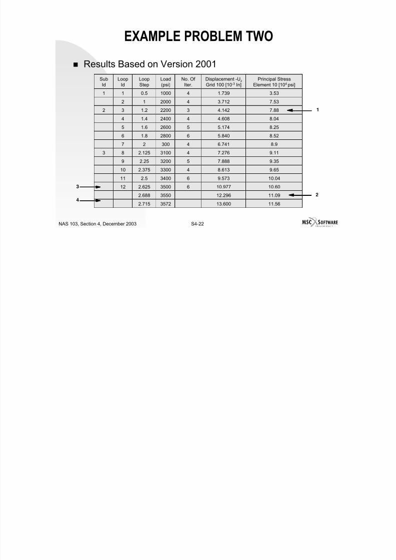
7/21/2019 Nonlinear Analysis Using MSC.nastran
http://slidepdf.com/reader/full/nonlinear-analysis-using-mscnastran 167/783
S4-21NAS 103, Section 4, December 2003
Grid 1000
z
y
x
Elastoplastic buckling of imperfect spherical shell, hydrostatic pressure applied,periphery clamped, undeformed shape.
R
Shell Model (QUAD4, TRIA)
3500 < scr < 3600
EXAMPLE PROBLEM TWO
Results Based on Version 2001
3.531.739410000.511
Principal StressElement 10 [104 psi]
Displacement -Uz
Grid 100 [10-3 In]No. Of
Iter.Load(psi)
LoopStep
LoopId
SubId

7/21/2019 Nonlinear Analysis Using MSC.nastran
http://slidepdf.com/reader/full/nonlinear-analysis-using-mscnastran 168/783
S4-22NAS 103, Section 4, December 2003
11.5613.60035722.715
11.0912.29635502.68810.6010.977635002.62512
10.049.573634002.511
9.658.613433002.37510
9.357.888532002.259
9.117.276431002.125838.96.741430027
8.525.840628001.86
8.255.174526001.65
8.044.608424001.44
7.884.142322001.2327.533.7124200012
1
23
4
EXAMPLE PROBLEM TWO
1. Upper fiber starts yielding2. Upper and lower fibers yield
3. After LOOPID 12, the negative factor diagonal occurs the
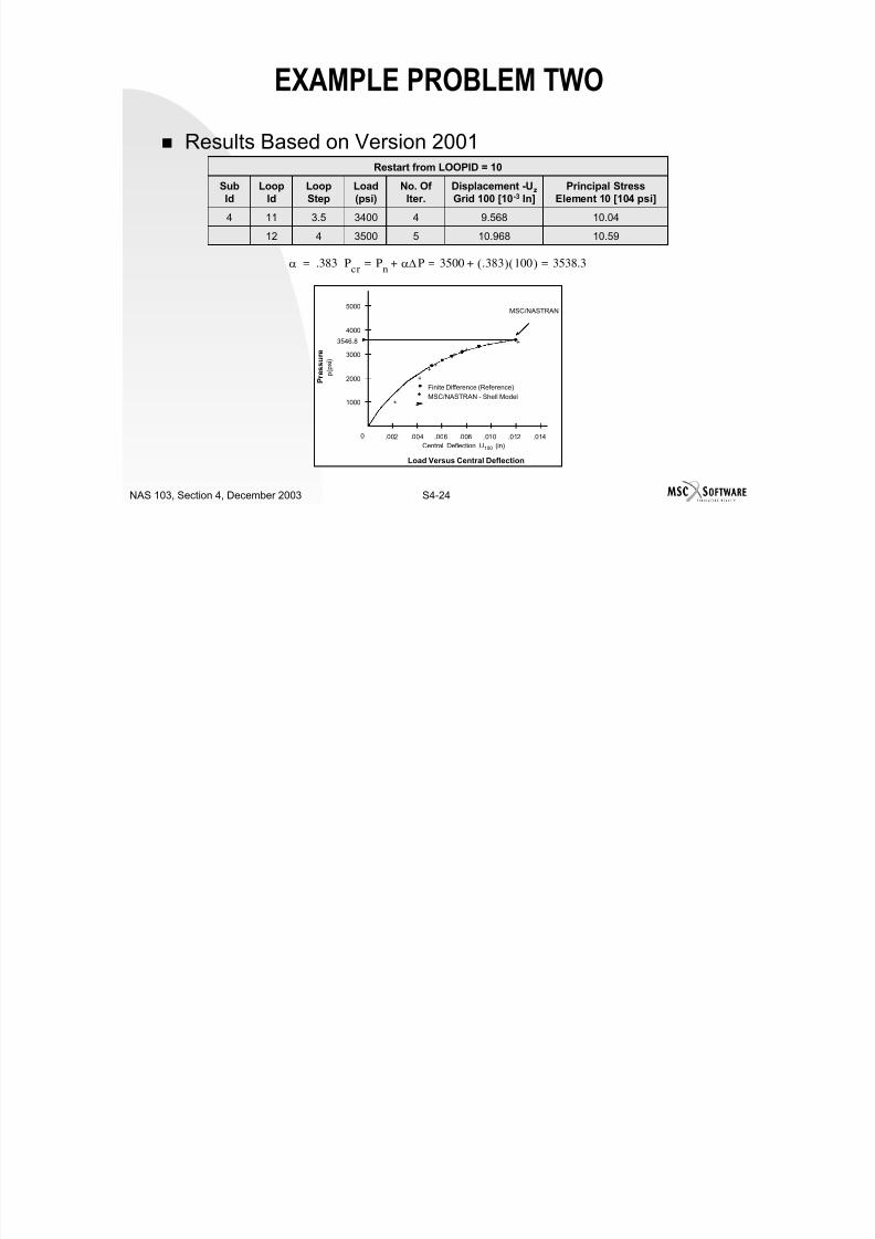
7/21/2019 Nonlinear Analysis Using MSC.nastran
http://slidepdf.com/reader/full/nonlinear-analysis-using-mscnastran 169/783
S4-23NAS 103, Section 4, December 2003
first time4. Last converged solution after several bisections
EXAMPLE PROBLEM TWO
Results Based on Version 2001
10.049.568434003.5114
Principal StressElement 10 [104 psi]
Displacement -Uz
Grid 100 [10-3 In]No. Of
Iter.Load(psi)
LoopStep
LoopId
SubId
Restart from LOOPID = 10

7/21/2019 Nonlinear Analysis Using MSC.nastran
http://slidepdf.com/reader/full/nonlinear-analysis-using-mscnastran 170/783
S4-24NAS 103, Section 4, December 2003
α .383 Pcr
Pn
= α∆P 3500 .383( ) 100( ) 3538.3=+=+=
10.5910.96853500412
Finite Difference (Reference)
MSC/NASTRAN - Shell Model
3546.8
5000
4000
3000
2000
1000
0 .002 .004 .006 .008 .010 .012 .014Central Deflection U100 (in)
p ( p s i )
Load Versus Central Deflection
P r e s s u r e
MSC/NASTRAN
+
++
++
+ + +
+
EXAMPLE PROBLEM TWO
Input File for Cold StartID SSBUK, NAS103 Example $ AR 12/03
SOL 106TIME 30
CENDTITLE=ELASTIC-PLASTIC BUCKLING OF IMPERFECT SPHERICAL SHELLSUBTITLE=HYDROSTATIC PRESSURE APPLIED, PERIPHERY CLAMPED
O 17 427 444 (1981)
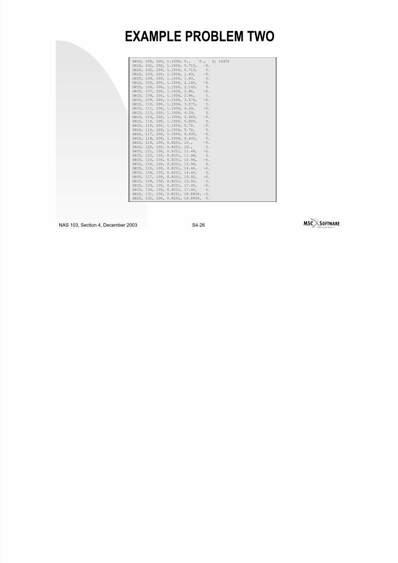
7/21/2019 Nonlinear Analysis Using MSC.nastran
http://slidepdf.com/reader/full/nonlinear-analysis-using-mscnastran 171/783
S4-25NAS 103, Section 4, December 2003
LABEL=REF.: KAO; IJNME; 17:427-444 (1981)ECHO=UNSORT
DISP(SORT2)=ALLOLOAD=ALLSPCF=ALL
STRESS(SORT2)=ALLSPC=10
SUBCASE 1LOAD=10NLPARM=10
SUBCASE 2LOAD=20NLPARM=20
SUBCASE 3
LOAD=30NLPARM=30
BEGIN BULK
$ DEFINE SPHERICAL COORDINATE SYSTEMSCORD2S, 100, , 0., 0., 0., 0., 0., 1., +C2S1
+C2S1, 1., 0., 1.
CORD2S, 200, , 0., 0., -.32908,0., 0., 1., +C2S2+C2S2, 1., 0, 1.
$ GEOMETRYGRDSET, , , , , , 100, 345
EXAMPLE PROBLEM TWO
GRID, 100, 200, 1.1506, 0., 0., 0, 12456GRID, 101, 200, 1.1506, 0.715, -5.GRID, 102, 200, 1.1506, 0.715, 5.GRID, 103, 200, 1.1506, 1.43, -5.
GRID, 104, 200, 1.1506, 1.43, 5.GRID, 105, 200, 1.1506, 2.145, -5.
GRID, 106, 200, 1.1506, 2.145, 5.GRID, 107, 200, 1.1506, 2.86, -5.GRID, 108, 200, 1.1506, 2.86, 5.
GRID, 109, 200, 1.1506, 3.575, -5.
GRID 110 200 1 1506 3 575 5
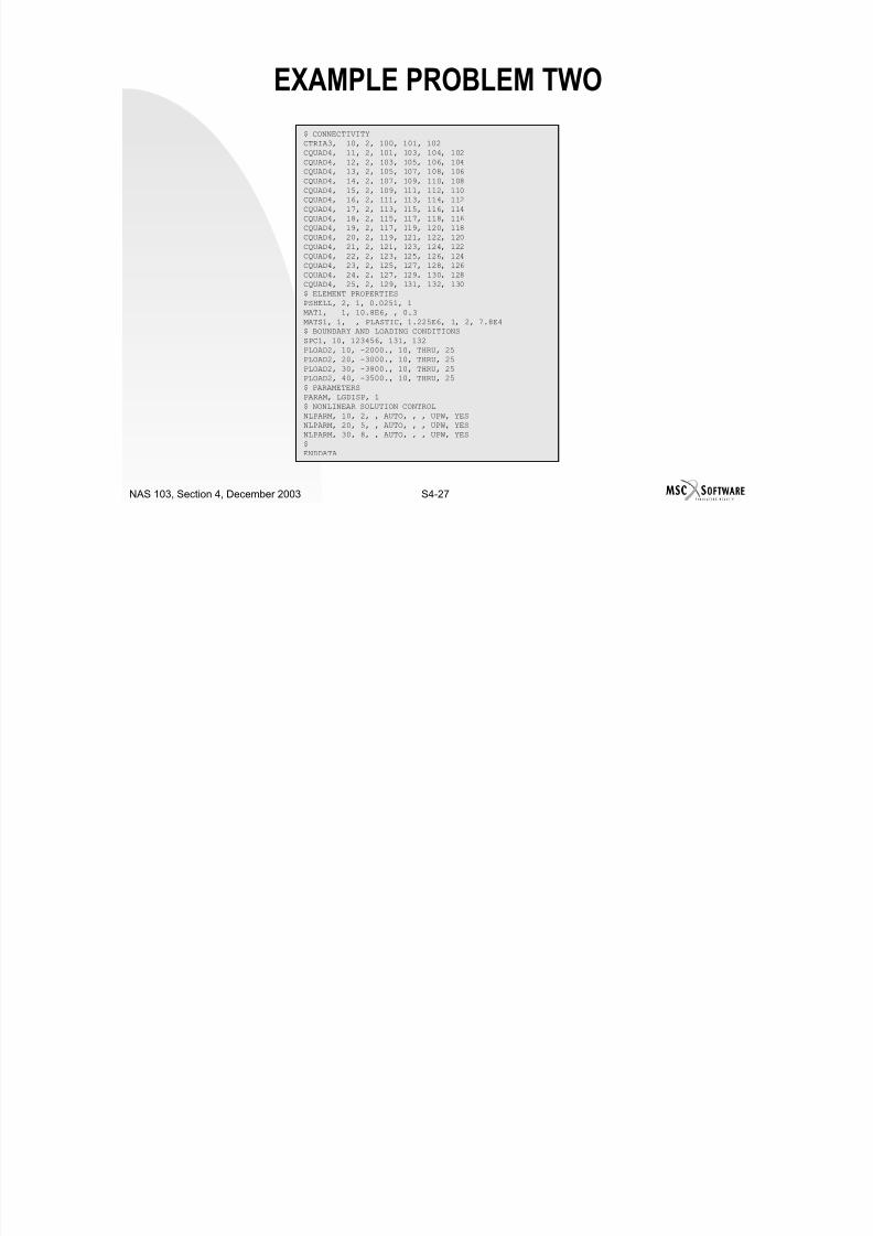
7/21/2019 Nonlinear Analysis Using MSC.nastran
http://slidepdf.com/reader/full/nonlinear-analysis-using-mscnastran 172/783
S4-26NAS 103, Section 4, December 2003
GRID, 110, 200, 1.1506, 3.575, 5.GRID, 111, 200, 1.1506, 4.29, -5.GRID, 112, 200, 1.1506, 4.29, 5.
GRID, 113, 200, 1.1506, 5.005, -5.GRID, 114, 200, 1.1506, 5.005, 5.
GRID, 115, 200, 1.1506, 5.72, -5.GRID, 116, 200, 1.1506, 5.72, 5.GRID, 117, 200, 1.1506, 6.435, -5.
GRID, 118, 200, 1.1506, 6.435, 5.GRID, 119, 100, 0.8251, 10., -5.
GRID, 120, 100, 0.8251, 10., 5.GRID, 121, 100, 0.8251, 11.48, -5.GRID, 122, 100, 0.8251, 11.48, 5.
GRID, 123, 100, 0.8251, 12.96, -5.GRID, 124, 100, 0.8251, 12.96, 5.GRID, 125, 100, 0.8251, 14.44, -5.GRID, 126, 100, 0.8251, 14.44, 5.GRID, 127, 100, 0.8251, 15.92, -5.
GRID, 128, 100, 0.8251, 15.92, 5.GRID, 129, 100, 0.8251, 17.40, -5.
GRID, 130, 100, 0.8251, 17.40, 5.GRID, 131, 100, 0.8251, 18.8806, -5.
GRID, 132, 100, 0.8251, 18.8806, 5.
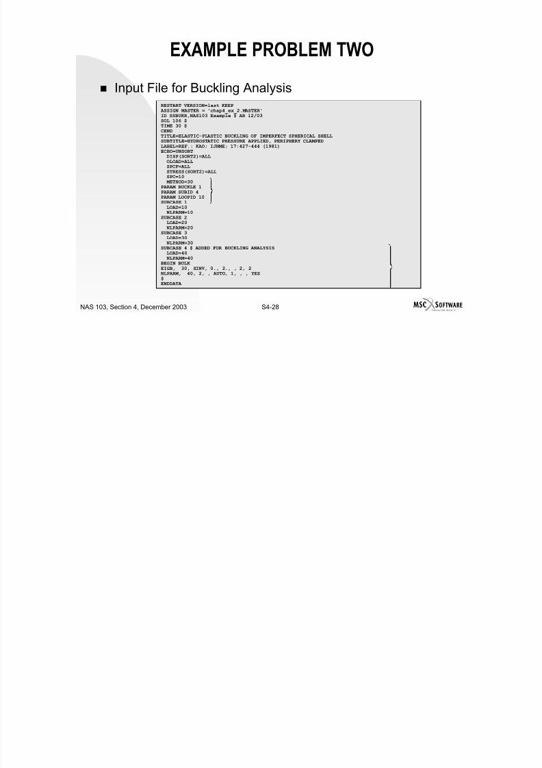
7/21/2019 Nonlinear Analysis Using MSC.nastran
http://slidepdf.com/reader/full/nonlinear-analysis-using-mscnastran 173/783
EXAMPLE PROBLEM TWO
Input File for Buckling AnalysisRESTART VERSION=last KEEP
ASSIGN MASTER = 'chap4_ex_2.MASTER'ID SSBUKR,NAS103 Example $ AR 12/03SOL 106 $TIME 30 $CENDTITLE=ELASTIC-PLASTIC BUCKLING OF IMPERFECT SPHERICAL SHELL
SUBTITLE=HYDROSTATIC PRESSURE APPLIED PERIPHERY CLAMPED1 2 (1981)

7/21/2019 Nonlinear Analysis Using MSC.nastran
http://slidepdf.com/reader/full/nonlinear-analysis-using-mscnastran 174/783
S4-28NAS 103, Section 4, December 2003
SUBTITLE=HYDROSTATIC PRESSURE APPLIED, PERIPHERY CLAMPEDLABEL=REF.: KAO; IJNME; 17:427-444 (1981)ECHO=UNSORTDISP(SORT2)=ALLOLOAD=ALLSPCF=ALLSTRESS(SORT2)=ALLSPC=10
METHOD=30PARAM BUCKLE 1PARAM SUBID 4PARAM LOOPID 10SUBCASE 1LOAD=10
NLPARM=10SUBCASE 2LOAD=20
NLPARM=20SUBCASE 3LOAD=30
NLPARM=30SUBCASE 4 $ ADDED FOR BUCKLING ANALYSISLOAD=40
NLPARM=40BEGIN BULKEIGB, 30, SINV, 0., 2., , 2, 2
NLPARM, 40, 2, , AUTO, 1, , , YES$ENDDATA
WORKSHOP PROBLEMS
Purpose To demonstrate use of (a) geometric nonlinear analysis, (b) linear and
nonlinear buckling analysis, and (c) arc length increments.
Problem DescriptionF th t t b l l l t

7/21/2019 Nonlinear Analysis Using MSC.nastran
http://slidepdf.com/reader/full/nonlinear-analysis-using-mscnastran 175/783
S4-29NAS 103, Section 4, December 2003
For the structure below, calculate:
100 = b
1 = zF
l
P, w EA = 107
Ks
WORKSHOP PROBLEMS
1. Linear Buckling load without spring.
2. Nonlinear Static with Large Deflection
3 N li B kli (PARAM BUCKLE 1)
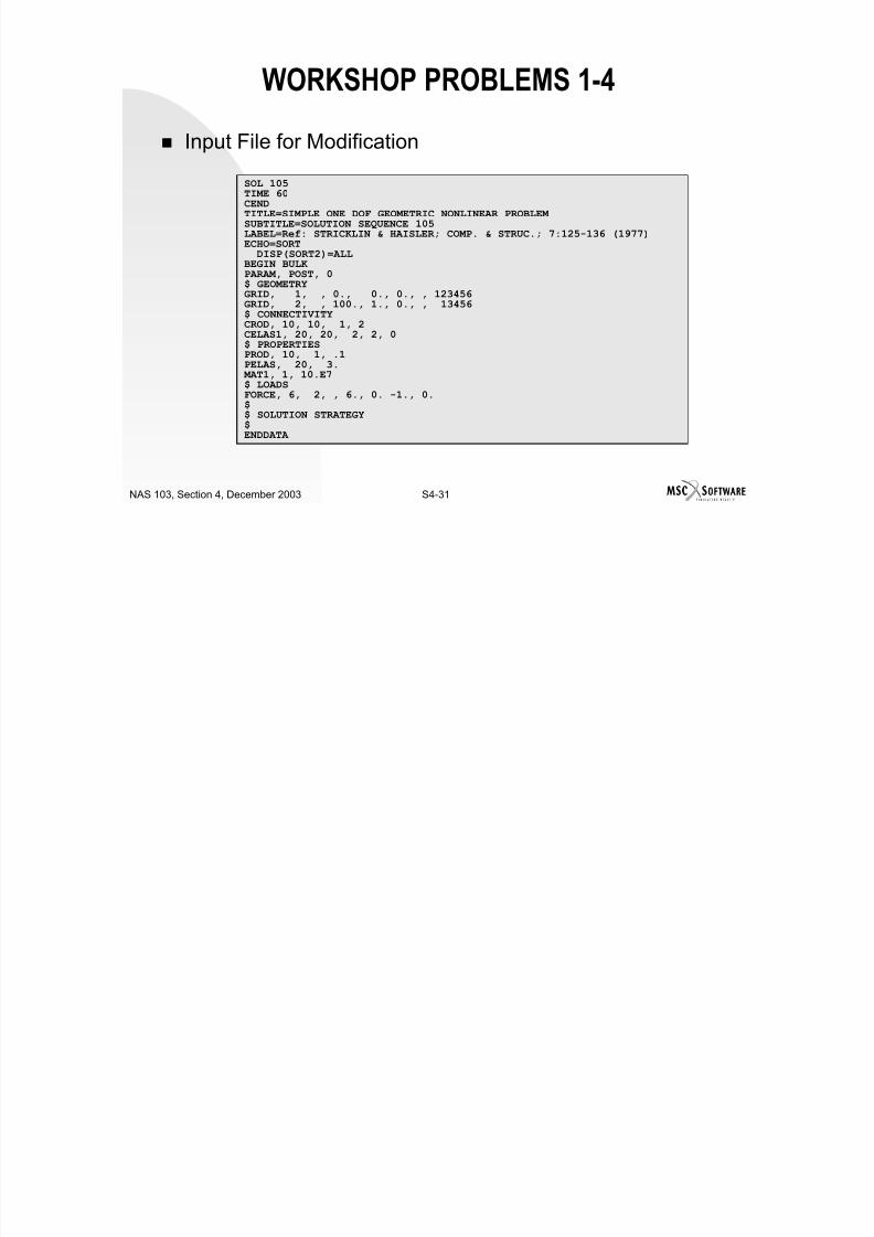
7/21/2019 Nonlinear Analysis Using MSC.nastran
http://slidepdf.com/reader/full/nonlinear-analysis-using-mscnastran 176/783
S4-30NAS 103, Section 4, December 2003
3. Nonlinear Buckling (PARAM, BUCKLE, 1)4. Nonlinear Static with Arc Length Method
5. Repeat above with spring (for Ks = 3, and 6)
WORKSHOP PROBLEMS 1-4
Input File for Modification
SOL 105TIME 60CENDTITLE=SIMPLE ONE DOF GEOMETRIC NONLINEAR PROBLEM
SUBTITLE=SOLUTION SEQUENCE 105LABEL=Ref: STRICKLIN & HAISLER; COMP. & STRUC.; 7:125-136 (1977)

7/21/2019 Nonlinear Analysis Using MSC.nastran
http://slidepdf.com/reader/full/nonlinear-analysis-using-mscnastran 177/783
S4-31NAS 103, Section 4, December 2003
Qe : S C & S ; CO . & S UC.; : 5 36 ( 9 )ECHO=SORTDISP(SORT2)=ALL
BEGIN BULKPARAM, POST, 0$ GEOMETRYGRID, 1, , 0., 0., 0., , 123456GRID, 2, , 100., 1., 0., , 13456$ CONNECTIVITY
CROD, 10, 10, 1, 2CELAS1, 20, 20, 2, 2, 0$ PROPERTIESPROD, 10, 1, .1PELAS, 20, 3. MAT1, 1, 10.E7$ LOADSFORCE, 6, 2, , 6., 0. -1., 0.$
$ SOLUTION STRATEGY$ENDDATA
SOLUTION FOR WORKSHOP PROBLEM ONE
1.
PblbPzFK
l
z
l
EA K
z Pl F
elastic
222
2
θsinP
∗=
≅≅
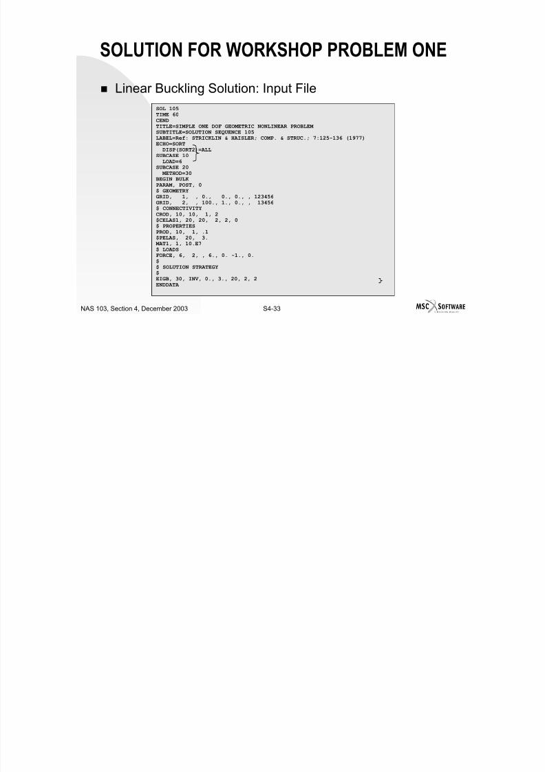
7/21/2019 Nonlinear Analysis Using MSC.nastran
http://slidepdf.com/reader/full/nonlinear-analysis-using-mscnastran 178/783
S4-32NAS 103, Section 4, December 2003
For
z l
Pb
z
l
l
b
l
P
l
z
l
F K geometric 2=∗
∗=
∗=
9995.9)100)(005.100(
1102
7
2
2
2
2
2
2
=∗
=
=
=
lb
EAz
z l
b
l
z
l
EA
P cr
SOLUTION FOR WORKSHOP PROBLEM ONE
Linear Buckling Solution: Input FileSOL 105TIME 60CENDTITLE=SIMPLE ONE DOF GEOMETRIC NONLINEAR PROBLEM SUBTITLE=SOLUTION SEQUENCE 105LABEL=Ref: STRICKLIN & HAISLER; COMP. & STRUC.; 7:125-136 (1977)
ECHO=SORTDISP(SORT2)=ALL
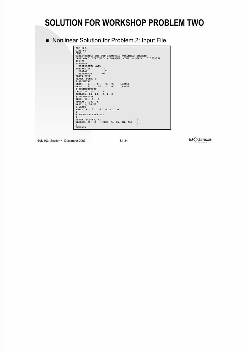
7/21/2019 Nonlinear Analysis Using MSC.nastran
http://slidepdf.com/reader/full/nonlinear-analysis-using-mscnastran 179/783
S4-33NAS 103, Section 4, December 2003
DISP(SORT2)=ALLSUBCASE 10LOAD=6
SUBCASE 20 METHOD=30BEGIN BULKPARAM, POST, 0$ GEOMETRYGRID, 1, , 0., 0., 0., , 123456
GRID, 2, , 100., 1., 0., , 13456$ CONNECTIVITYCROD, 10, 10, 1, 2$CELAS1, 20, 20, 2, 2, 0$ PROPERTIESPROD, 10, 1, .1$PELAS, 20, 3. MAT1, 1, 10.E7$ LOADSFORCE, 6, 2, , 6., 0. -1., 0.
$$ SOLUTION STRATEGY$EIGB, 30, INV, 0., 3., 20, 2, 2ENDDATA
SOLUTION FOR WORKSHOP PROBLEM TWO
Nonlinear Solution for Problem 2: Input FileSOL 106TIME 60CENDTITLE=SIMPLE ONE DOF GEOMETRIC NONLINEAR PROBLEM LABEL=Ref: STRICKLIN & HAISLER; COMP. & STRUC.; 7:125-136(1977)ECHO=SORTDISP(SORT2)=ALL
SUBCASE 10

7/21/2019 Nonlinear Analysis Using MSC.nastran
http://slidepdf.com/reader/full/nonlinear-analysis-using-mscnastran 180/783
S4-34NAS 103, Section 4, December 2003
SUBCASE 10LOAD=6 NLPARM=20BEGIN BULKPARAM, POST, 0$ GEOMETRYGRID, 1, , 0., 0., 0., , 123456GRID, 2, , 100., 1., 0., , 13456$ CONNECTIVITY
CROD, 10, 10, 1, 2$CELAS1, 20, 20, 2, 2, 0$ PROPERTIESPROD, 10, 1, .1$PELAS, 20, 3. MAT1, 1, 10.E7$ LOADSFORCE, 6, 2, , 6., 0. -1., 0.$$ SOLUTION STRATEGY$PARAM, LGDISP, +1 NLPARM, 20, 10, , ITER, 5, 25, PW, ALL$ENDDATA
SOLUTION FOR WORKSHOP PROBLEM THREE
RESTART,VERSION=1,KEEP ASSIGN MASTER='chap4_ws_2s.MASTER'TIME 60 $SOL 106$CENDTITLE=SIMPLE ONE DOF GEOMETRIC NONLINEAR PROBLEM LABEL=Ref: STRICKLIN & HAISLER; COMP. & STRUC.; 7:125-136 (1977)ECHO=SORTDISP(SORT2)=ALL
PARAM,LOOPID,3PARAM,SUBID,2

7/21/2019 Nonlinear Analysis Using MSC.nastran
http://slidepdf.com/reader/full/nonlinear-analysis-using-mscnastran 181/783
S4-35NAS 103, Section 4, December 2003
, , METHOD,30SUBCASE 10LOAD=6 NLPARM=20SUBCASE 20LOAD=6 NLPARM=30
BEGIN BULKPARAM, BUCKLE, 1EIGB, 30, INV, 0., 3., 20, 2, 2 NLPARM, 30, 70, , ITER, 1, 25, PW, ALLENDDATA
RESULTS FOR WORKSHOP PROBLEMS 1 - 3
Linear Buckling Vs. Nonlinear Buckling Solution:
Pcr (Nonlinear)
PARAM, BUCKLE, 1
Pcr (Linear)
SOL 105
Ks
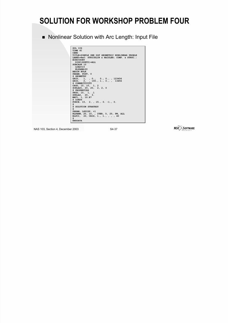
7/21/2019 Nonlinear Analysis Using MSC.nastran
http://slidepdf.com/reader/full/nonlinear-analysis-using-mscnastran 182/783
S4-36NAS 103, Section 4, December 2003
3.43616.9003
1.9249.9990
N/A25.6016
SOLUTION FOR WORKSHOP PROBLEM FOUR
Nonlinear Solution with Arc Length: Input File
SOL 106TIME 60CENDTITLE=SIMPLE ONE DOF GEOMETRIC NONLINEAR PROBLELABEL=Ref: STRICKLIN & HAISLER; COMP. & STRUC.;
ECHO=SORTDISP(SORT2)=ALLSUBCASE 10
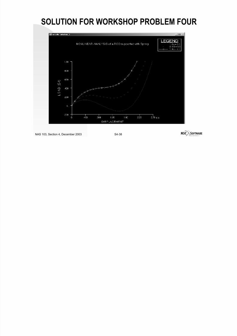
7/21/2019 Nonlinear Analysis Using MSC.nastran
http://slidepdf.com/reader/full/nonlinear-analysis-using-mscnastran 183/783
S4-37NAS 103, Section 4, December 2003
SUBCASE 10LOAD=15 NLPARM=20BEGIN BULKPARAM, POST, 0$ GEOMETRYGRID, 1, , 0., 0., 0., , 123456GRID, 2, , 100., 1., 0., , 13456$ CONNECTIVITYCROD, 10, 10, 1, 2$CELAS1, 20, 20, 2, 2, 0$ PROPERTIESPROD, 10, 1, .1$PELAS, 20, 3. MAT1, 1, 10.E7$ LOADSFORCE, 15, 2, , 15., 0. -1., 0.$$ SOLUTION STRATEGY
$PARAM, LGDISP, +1 NLPARM, 20, 10, , ITER, 5, 25, PW, ALL NLPCI, 20, CRIS, 1., 1., , , , 40$ENDDATA
SOLUTION FOR WORKSHOP PROBLEM FOUR

7/21/2019 Nonlinear Analysis Using MSC.nastran
http://slidepdf.com/reader/full/nonlinear-analysis-using-mscnastran 184/783
S4-38NAS 103, Section 4, December 2003
SECTION 5
MATERIAL NONLINEAR ANALYSIS

7/21/2019 Nonlinear Analysis Using MSC.nastran
http://slidepdf.com/reader/full/nonlinear-analysis-using-mscnastran 185/783
S5-1NAS103, Section 5, February 2004

7/21/2019 Nonlinear Analysis Using MSC.nastran
http://slidepdf.com/reader/full/nonlinear-analysis-using-mscnastran 186/783
S5-2NAS103, Section 5, February 2004
TABLE OF CONTENTSPage
Material Types in MSC.Nastran 5-5Nonlinear Elasticity 5-11
Workshop Problem 1: Nonlinear Elastic Material 5-27
Hyperelasticity 5-33
Workshop Problem 2: Hyperelastic Material 5-45

7/21/2019 Nonlinear Analysis Using MSC.nastran
http://slidepdf.com/reader/full/nonlinear-analysis-using-mscnastran 187/783
S5-3NAS103, Section 5, February 2004
p ypElastic-Plastic Material 5-53
Workshop Problem 3: Elastic-Plastic Material 5-73
Creep (Viscoelastic) Material 5-81
Workshop Problem 4: Creep Material 5-96
Workshop Problem 5: Temperature Dependent Mat. 5-105
Workshop Problem 6: Elastic-Pefectly Plastic Mat. 5-111
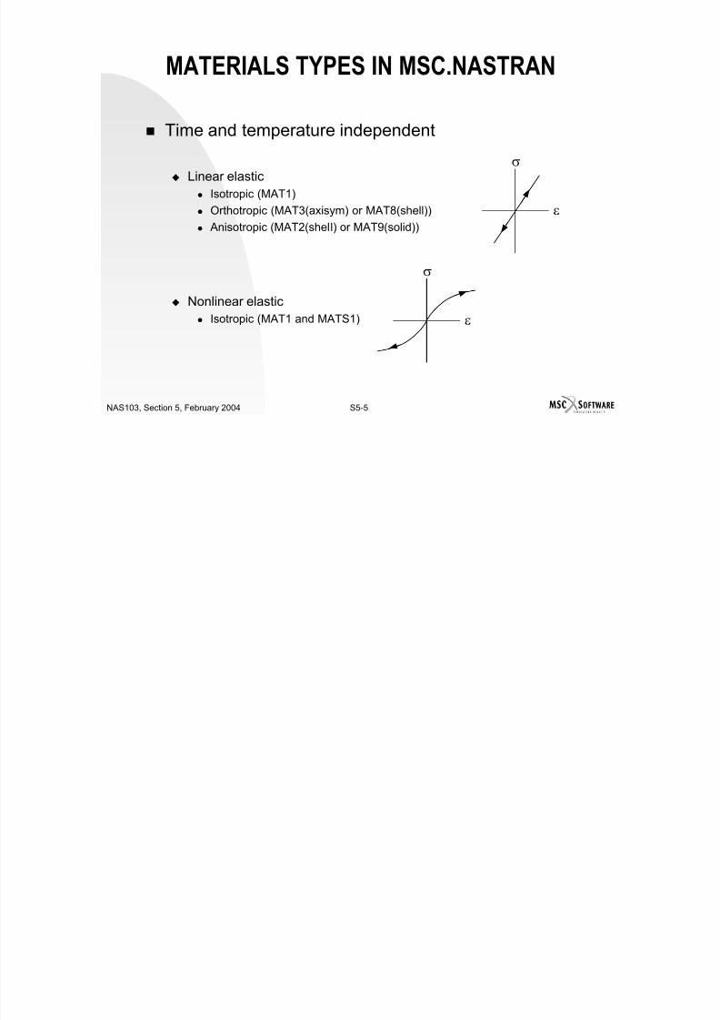
7/21/2019 Nonlinear Analysis Using MSC.nastran
http://slidepdf.com/reader/full/nonlinear-analysis-using-mscnastran 188/783
S5-4NAS103, Section 5, February 2004
MATERIALS TYPES IN MSC.NASTRAN
Time and temperature independent
Linear elastic Isotropic (MAT1)
Orthotropic (MAT3(axisym) or MAT8(shell)) ε
σ
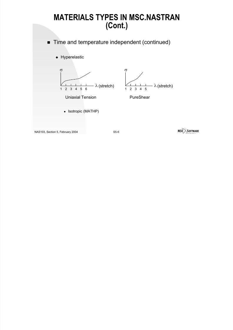
7/21/2019 Nonlinear Analysis Using MSC.nastran
http://slidepdf.com/reader/full/nonlinear-analysis-using-mscnastran 189/783
S5-5NAS103, Section 5, February 2004
Orthotropic (MAT3(axisym) or MAT8(shell))
Anisotropic (MAT2(shell) or MAT9(solid))
Nonlinear elastic Isotropic (MAT1 and MATS1)
ε
σ
ε
MATERIALS TYPES IN MSC.NASTRAN(Cont.)
Time and temperature independent (continued)
Hyperelastic

7/21/2019 Nonlinear Analysis Using MSC.nastran
http://slidepdf.com/reader/full/nonlinear-analysis-using-mscnastran 190/783
S5-6NAS103, Section 5, February 2004
Isotropic (MATHP)
σ
λ1 2 3 4 5 6 (stretch)
Uniaxial Tension
σ
λ1 2 3 4 5 (stretch)
PureShear
MATERIALS TYPES IN MSC.NASTRAN(Cont.)
Time and temperature independent (continued)
Elastic-plastic
σ σ
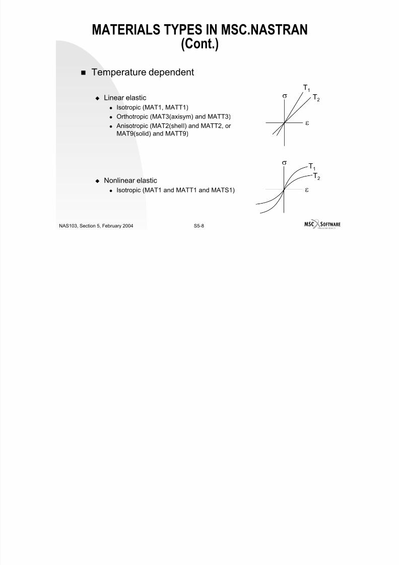
7/21/2019 Nonlinear Analysis Using MSC.nastran
http://slidepdf.com/reader/full/nonlinear-analysis-using-mscnastran 191/783
S5-7NAS103, Section 5, February 2004
Isotropic (MAT1, MATS1) Anisotropic (MAT2(shell) or MAT9(solid), and MATS1)
ε
σ
Perfectly Plastic Linear Strain Hardening
ε
σ
MATERIALS TYPES IN MSC.NASTRAN(Cont.)
Temperature dependent
Linear elastic Isotropic (MAT1, MATT1) Orthotropic (MAT3(axisym) and MATT3)
σ T2
T1
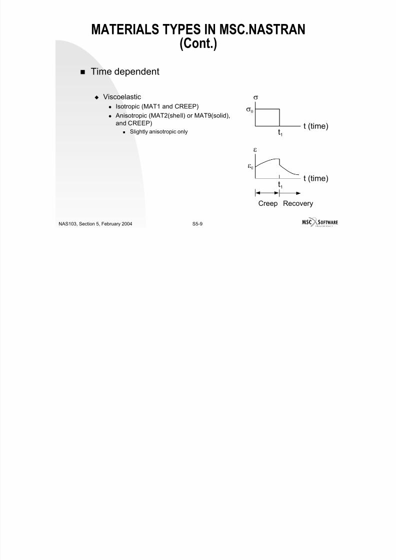
7/21/2019 Nonlinear Analysis Using MSC.nastran
http://slidepdf.com/reader/full/nonlinear-analysis-using-mscnastran 192/783
S5-8NAS103, Section 5, February 2004
Orthotropic (MAT3(axisym) and MATT3)
Anisotropic (MAT2(shell) and MATT2, orMAT9(solid) and MATT9)
Nonlinear elastic
Isotropic (MAT1 and MATT1 and MATS1)
ε
σ
ε
T2
T1
MATERIALS TYPES IN MSC.NASTRAN(Cont.)
Time dependent
Viscoelastic Isotropic (MAT1 and CREEP) Anisotropic (MAT2(shell) or MAT9(solid),
σ
σ0

7/21/2019 Nonlinear Analysis Using MSC.nastran
http://slidepdf.com/reader/full/nonlinear-analysis-using-mscnastran 193/783
S5-9NAS103, Section 5, February 2004
Anisotropic (MAT2(shell) or MAT9(solid),and CREEP)
Slightly anisotropic onlyt (time)
t1
ε
t (time)
ε0
t1
Creep Recovery
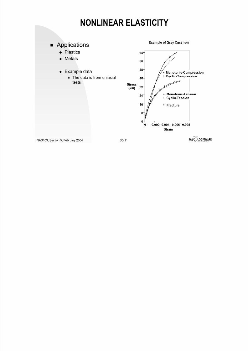
7/21/2019 Nonlinear Analysis Using MSC.nastran
http://slidepdf.com/reader/full/nonlinear-analysis-using-mscnastran 194/783
NONLINEAR ELASTICITY
Applications Plastics
Metals
Example data
7/21/2019 Nonlinear Analysis Using MSC.nastran
http://slidepdf.com/reader/full/nonlinear-analysis-using-mscnastran 195/783
S5-11NAS103, Section 5, February 2004
The data is from uniaxialtests
NONLINEAR ELASTICITY (Cont.)
Limitations in MSC.Nastran Small strain
Isotropic materials only
No time dependence – no creep Can use beam element, but not recommended to use offset
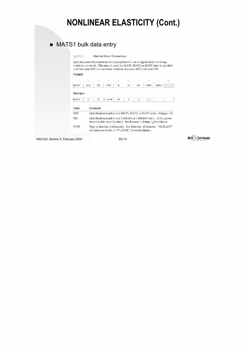
7/21/2019 Nonlinear Analysis Using MSC.nastran
http://slidepdf.com/reader/full/nonlinear-analysis-using-mscnastran 196/783
S5-12NAS103, Section 5, February 2004
vectors, in solution sequences that use differential stiffness,because the vectors do not change angle(orientation)
User interface MAT1 used to specify E, G, ν, ρ
ΜΑΤΤ1 used to specify temperature dependence of E, G, ν, ρ
ΜΑΤS1 used, along with table TABLES1 or TABLEST(temperature dependence), to specify stress versus strain (fromuniaxial test)
NONLINEAR ELASTICITY (Cont.)
MATS1 bulk data entry
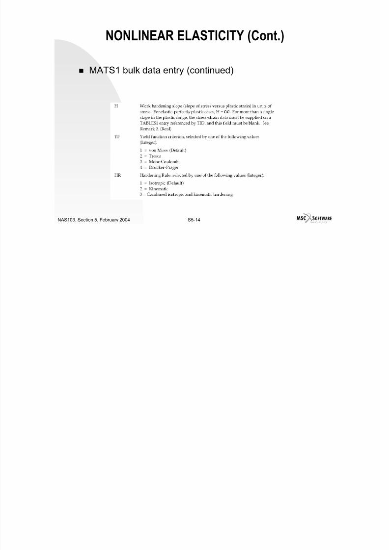
7/21/2019 Nonlinear Analysis Using MSC.nastran
http://slidepdf.com/reader/full/nonlinear-analysis-using-mscnastran 197/783
S5-13NAS103, Section 5, February 2004
NONLINEAR ELASTICITY (Cont.)
MATS1 bulk data entry (continued)
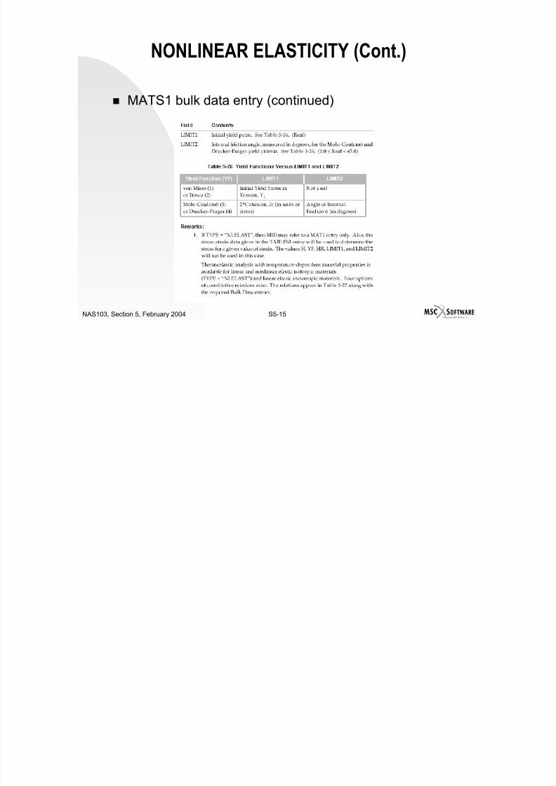
7/21/2019 Nonlinear Analysis Using MSC.nastran
http://slidepdf.com/reader/full/nonlinear-analysis-using-mscnastran 198/783
S5-14NAS103, Section 5, February 2004
NONLINEAR ELASTICITY (Cont.)
MATS1 bulk data entry (continued)
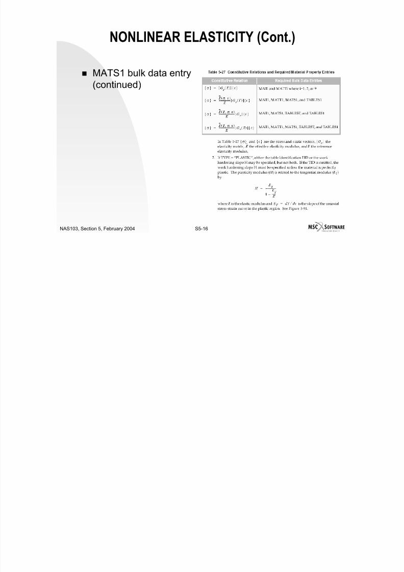
7/21/2019 Nonlinear Analysis Using MSC.nastran
http://slidepdf.com/reader/full/nonlinear-analysis-using-mscnastran 199/783
S5-15NAS103, Section 5, February 2004
NONLINEAR ELASTICITY (Cont.)
MATS1 bulk data entry(continued)
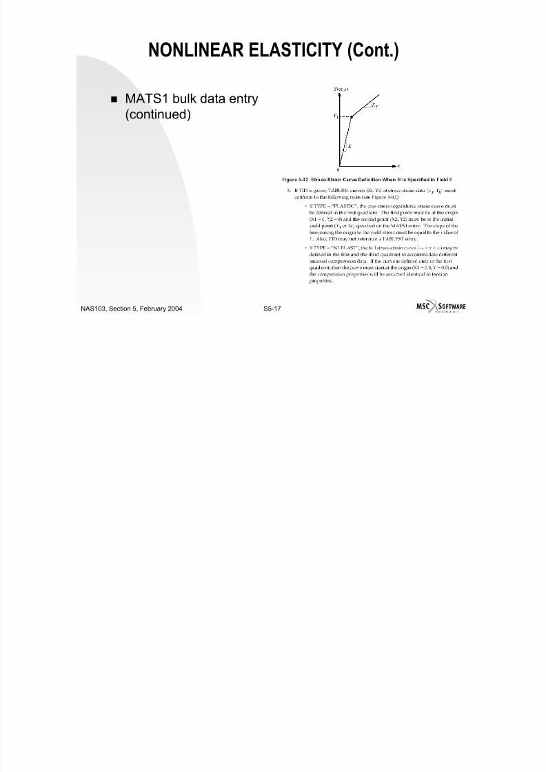
7/21/2019 Nonlinear Analysis Using MSC.nastran
http://slidepdf.com/reader/full/nonlinear-analysis-using-mscnastran 200/783
S5-16NAS103, Section 5, February 2004
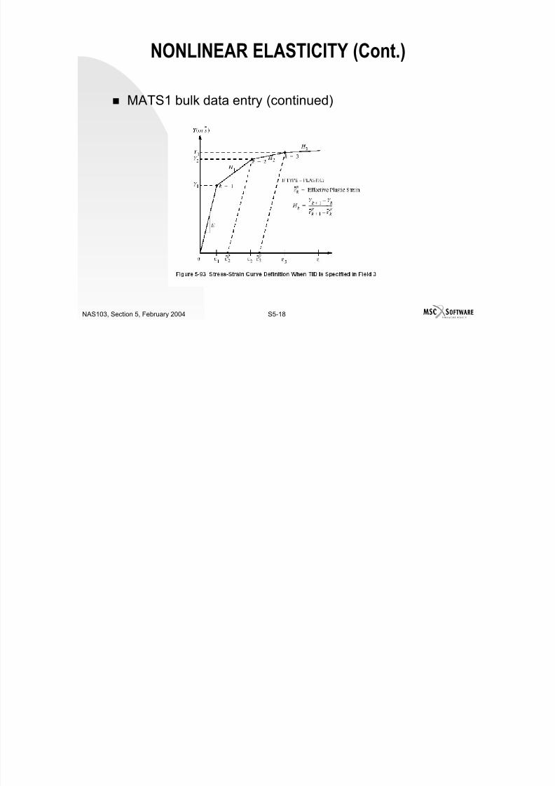
7/21/2019 Nonlinear Analysis Using MSC.nastran
http://slidepdf.com/reader/full/nonlinear-analysis-using-mscnastran 201/783
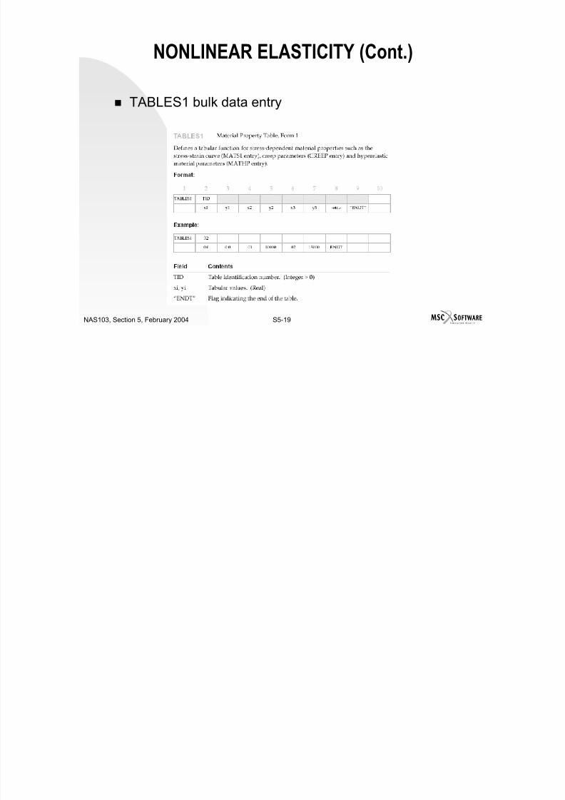
7/21/2019 Nonlinear Analysis Using MSC.nastran
http://slidepdf.com/reader/full/nonlinear-analysis-using-mscnastran 202/783
NONLINEAR ELASTICITY (Cont.)
TABLES1 bulk data entry

7/21/2019 Nonlinear Analysis Using MSC.nastran
http://slidepdf.com/reader/full/nonlinear-analysis-using-mscnastran 203/783
S5-19NAS103, Section 5, February 2004
NONLINEAR ELASTICITY (Cont.)
TABLES1 bulk data entry (continued)
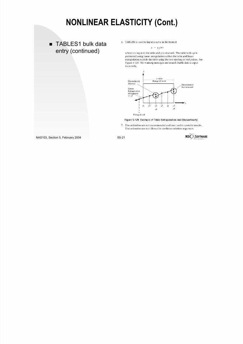
7/21/2019 Nonlinear Analysis Using MSC.nastran
http://slidepdf.com/reader/full/nonlinear-analysis-using-mscnastran 204/783
S5-20NAS103, Section 5, February 2004
NONLINEAR ELASTICITY (Cont.)
TABLES1 bulk dataentry (continued)
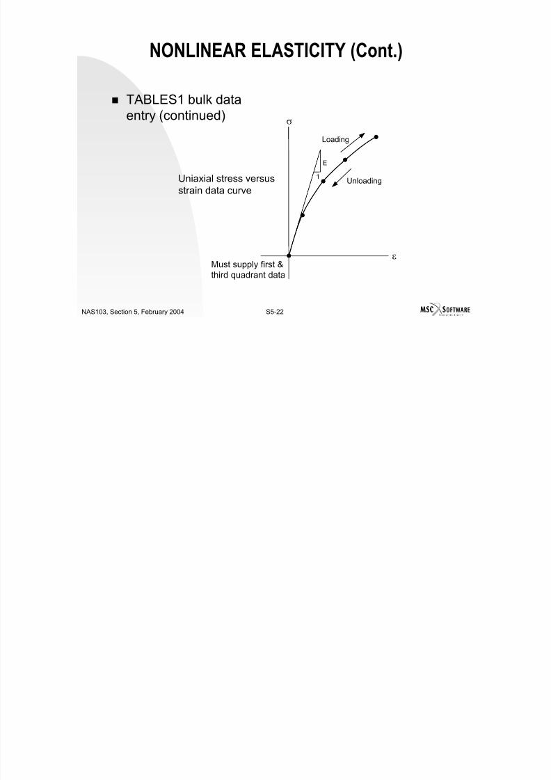
7/21/2019 Nonlinear Analysis Using MSC.nastran
http://slidepdf.com/reader/full/nonlinear-analysis-using-mscnastran 205/783
S5-21NAS103, Section 5, February 2004
NONLINEAR ELASTICITY (Cont.)
TABLES1 bulk dataentry (continued)
1
E
σ
Loading

7/21/2019 Nonlinear Analysis Using MSC.nastran
http://slidepdf.com/reader/full/nonlinear-analysis-using-mscnastran 206/783
S5-22NAS103, Section 5, February 2004
1
ε
Unloading
Must supply first &third quadrant data
Uniaxial stress versusstrain data curve
NONLINEAR ELASTICITY, RELATIONBETWEEN UNIAXIAL AND MULTIAXIAL
Following are remarks on stress and strain data from auniaxial test, and how it relates to the multiaxial stressand strain state as simulated by MSC.Nastran
As previously mentioned, the stress and strain dataused for the TABLES1 entry is from a uniaxial test(s)
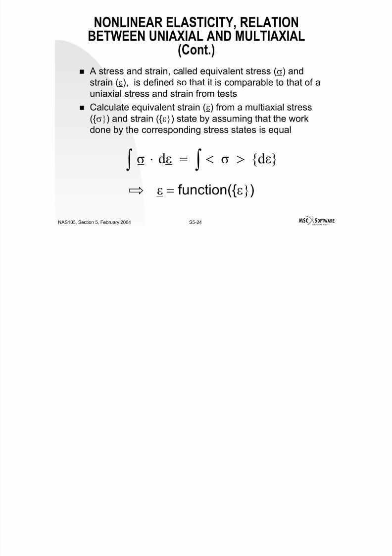
7/21/2019 Nonlinear Analysis Using MSC.nastran
http://slidepdf.com/reader/full/nonlinear-analysis-using-mscnastran 207/783
S5-23NAS103, Section 5, February 2004
The simulation by MSC.Nastran is not uniaxial, butmultiaxial
How does MSC.Nastran use the uniaxial data ?
A stress and strain, called equivalent stress (σ) andstrain (ε), is defined so that it is comparable to that of auniaxial stress and strain from tests
Calculate equivalent strain (ε) from a multiaxial stress(σ) and strain (ε) state by assuming that the work
NONLINEAR ELASTICITY, RELATIONBETWEEN UNIAXIAL AND MULTIAXIAL
(Cont.)
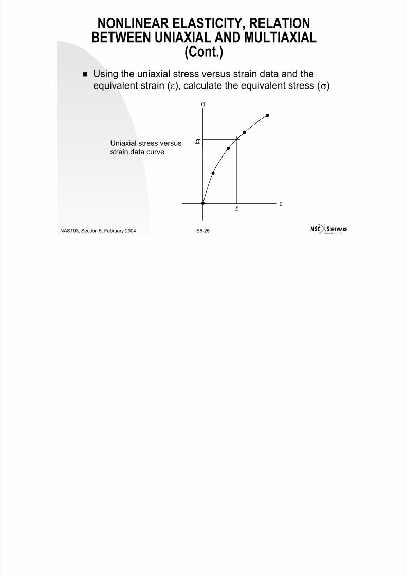
7/21/2019 Nonlinear Analysis Using MSC.nastran
http://slidepdf.com/reader/full/nonlinear-analysis-using-mscnastran 208/783
S5-24NAS103, Section 5, February 2004
done by the corresponding stress states is equal
dεσdεσ ∫∫ ><=⋅
ε = function(ε)
Using the uniaxial stress versus strain data and theequivalent strain (ε), calculate the equivalent stress (σ)
NONLINEAR ELASTICITY, RELATIONBETWEEN UNIAXIAL AND MULTIAXIAL
(Cont.)
σ
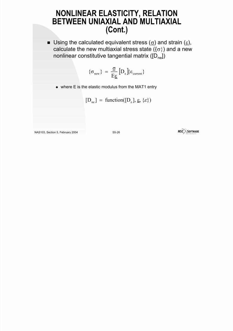
7/21/2019 Nonlinear Analysis Using MSC.nastran
http://slidepdf.com/reader/full/nonlinear-analysis-using-mscnastran 209/783
S5-25NAS103, Section 5, February 2004
Uniaxial stress versus
strain data curve
ε
σ
ε
Using the calculated equivalent stress (σ) and strain (ε),calculate the new multiaxial stress state (σ) and a newnonlinear constitutive tangential matrix ([Dne])
NONLINEAR ELASTICITY, RELATIONBETWEEN UNIAXIAL AND MULTIAXIAL
(Cont.)
[ ] εDEε
σσ currentenew =

7/21/2019 Nonlinear Analysis Using MSC.nastran
http://slidepdf.com/reader/full/nonlinear-analysis-using-mscnastran 210/783
S5-26NAS103, Section 5, February 2004
where E is the elastic modulus from the MAT1 entry
Eε
)ε,],Dfunction([][D ene ε =
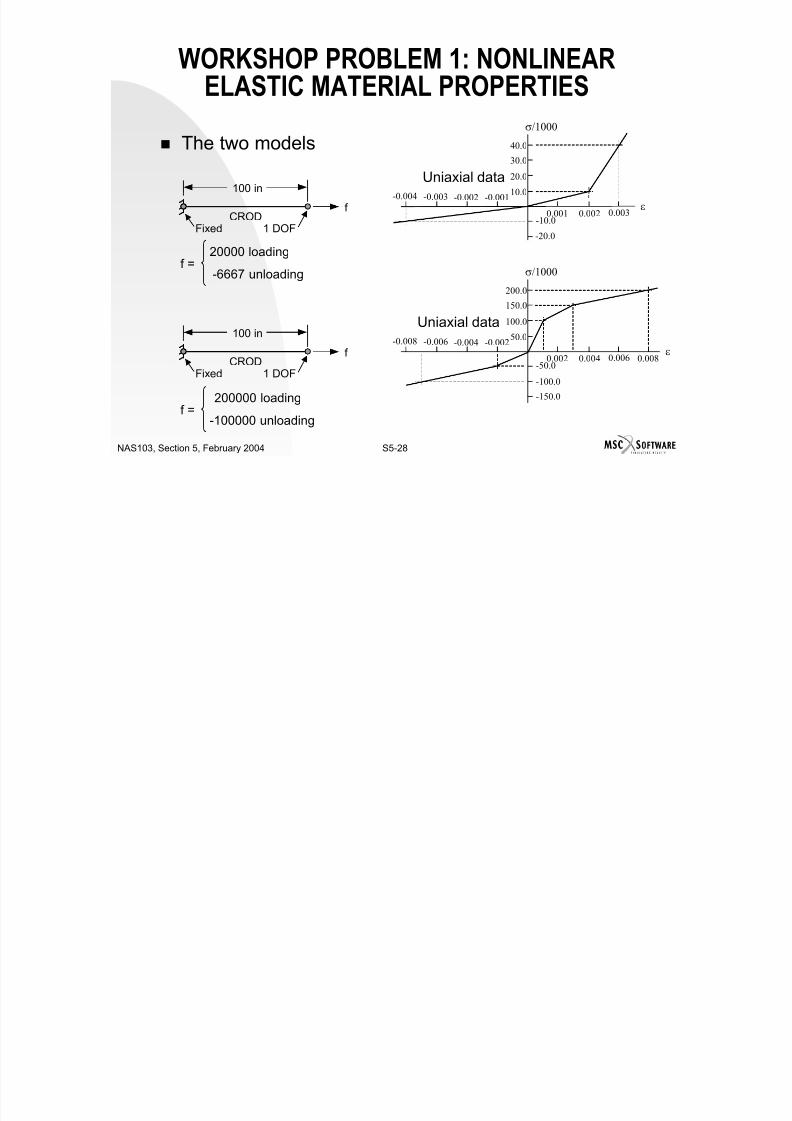
7/21/2019 Nonlinear Analysis Using MSC.nastran
http://slidepdf.com/reader/full/nonlinear-analysis-using-mscnastran 211/783

7/21/2019 Nonlinear Analysis Using MSC.nastran
http://slidepdf.com/reader/full/nonlinear-analysis-using-mscnastran 212/783
Include in model SOL 106
A subcase for loading, and a subcase for unloading
The bulk data entry NLPARM, and corresponding case control entry
Material entries for linear and nonlinear elastic properties
WORKSHOP PROBLEM 1: NONLINEARELASTIC MATERIAL PROPERTIES

7/21/2019 Nonlinear Analysis Using MSC.nastran
http://slidepdf.com/reader/full/nonlinear-analysis-using-mscnastran 213/783
S5-29NAS103, Section 5, February 2004
WORKSHOP PROBLEM 1: NONLINEARELASTIC MATERIAL PROPERTIES
Input File for Modification
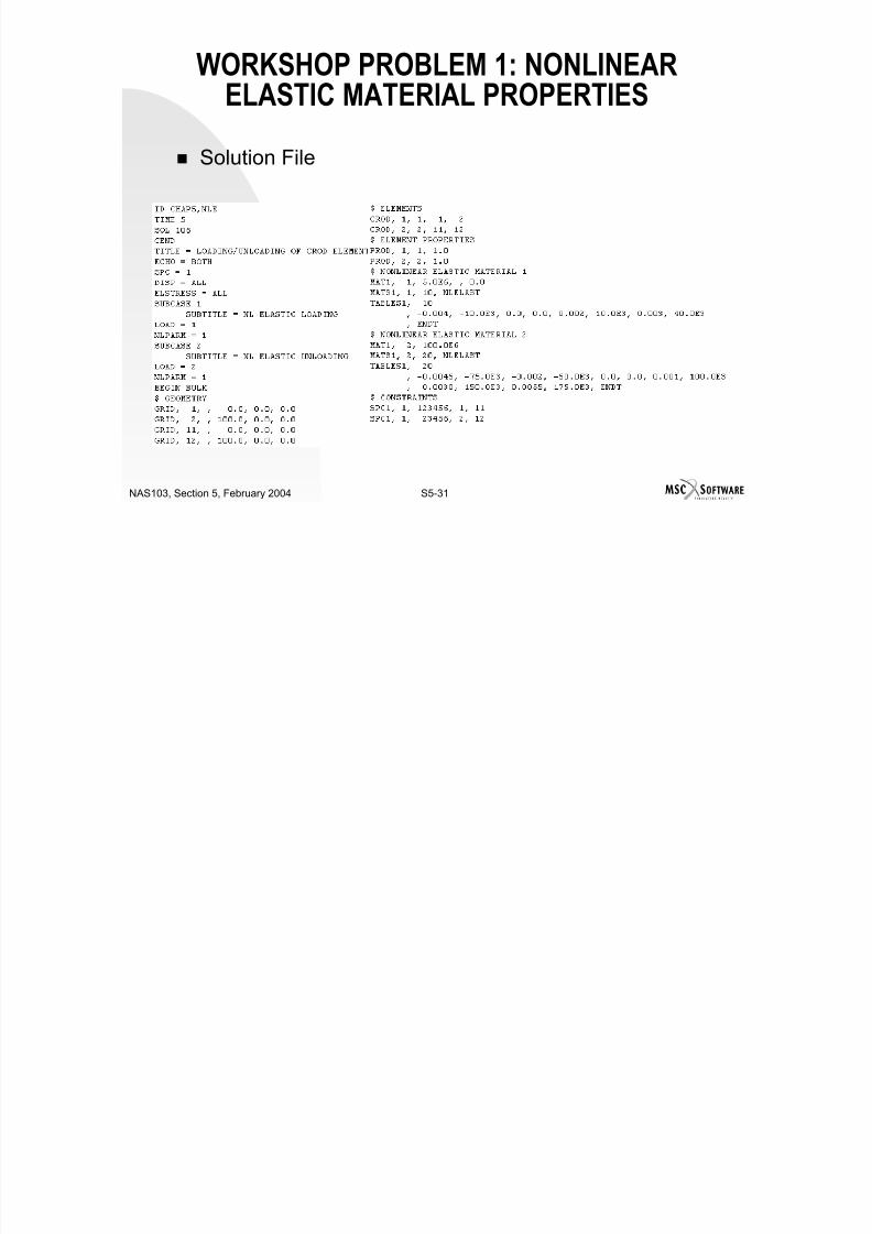
7/21/2019 Nonlinear Analysis Using MSC.nastran
http://slidepdf.com/reader/full/nonlinear-analysis-using-mscnastran 214/783
S5-30NAS103, Section 5, February 2004

7/21/2019 Nonlinear Analysis Using MSC.nastran
http://slidepdf.com/reader/full/nonlinear-analysis-using-mscnastran 215/783
WORKSHOP PROBLEM 1: NONLINEARELASTIC MATERIAL PROPERTIES
Solution File (continued)

7/21/2019 Nonlinear Analysis Using MSC.nastran
http://slidepdf.com/reader/full/nonlinear-analysis-using-mscnastran 216/783
S5-32NAS103, Section 5, February 2004
HYPERELASTICITY
Definition Materials that exhibit elastic behavior through large strains
Described using a scalar strain energy function
Derivative of strain energy function with respect to a strain componentdetermines the corresponding stress component
A li ti f d l t t l t i l
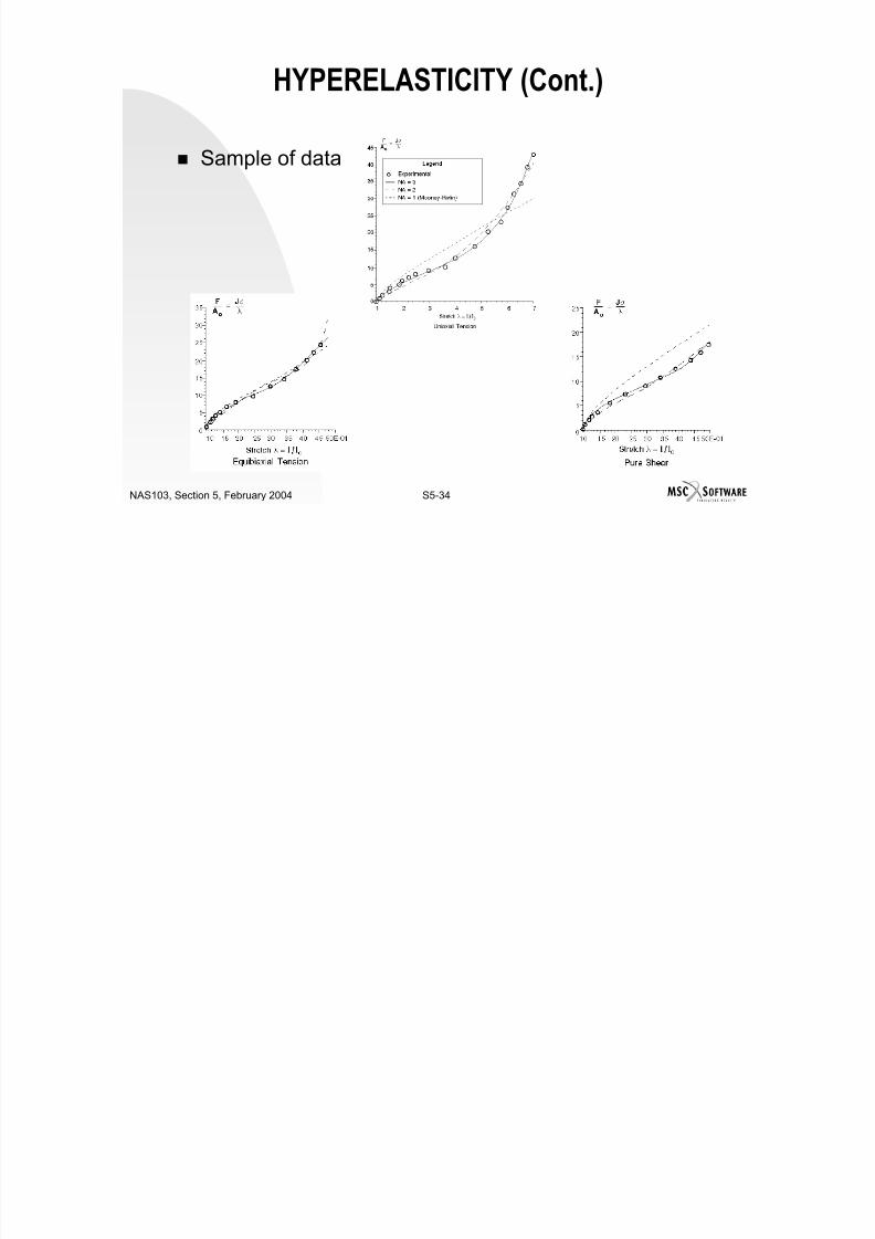
7/21/2019 Nonlinear Analysis Using MSC.nastran
http://slidepdf.com/reader/full/nonlinear-analysis-using-mscnastran 217/783
S5-33NAS103, Section 5, February 2004
Application of model to actual materials Rubber material: O-rings, bushings, gaskets, seals, boots, tires
Plastic
Glass
Solid propellant
Other elastomers
HYPERELASTICITY (Cont.)
Sample of data

7/21/2019 Nonlinear Analysis Using MSC.nastran
http://slidepdf.com/reader/full/nonlinear-analysis-using-mscnastran 218/783
S5-34NAS103, Section 5, February 2004
HYPERELASTICITY (Cont.)
Limitations of MSC.Nastran Fully incompressible material (ν = 0.5) not currently implemented
Acceptable for nearly incompressible materials, e.g. ν = 0.4995

7/21/2019 Nonlinear Analysis Using MSC.nastran
http://slidepdf.com/reader/full/nonlinear-analysis-using-mscnastran 219/783
S5-35NAS103, Section 5, February 2004
HYPERELASTICITY (Cont.)
Comments on formulation of constitutive materialproperties
whereS d Pi l Ki hh ff t t t i t ith t
C
W2S
∂
∂=

7/21/2019 Nonlinear Analysis Using MSC.nastran
http://slidepdf.com/reader/full/nonlinear-analysis-using-mscnastran 220/783
S5-36NAS103, Section 5, February 2004
S = second Piola-Kirchhoff stress tensor; symmetric stress with respectto undeformed state
C = right Cauchy-Green strain tensor W = elastic strain energy function; generalized Mooney-Rivlin model
∑∑ −−−+−−=
ND
i
2i
0vi
j
2
i
1
NA
ji, ij
))T(T1(JD3)(I3)(IAW α
HYPERELASTICITY (Cont.)
The coefficients Aij and Di are determined usingexperimental data Aij = coefficients accounting for distortion
Di = coefficients accounting for volumetric change Tests performed are
Distortional deformation
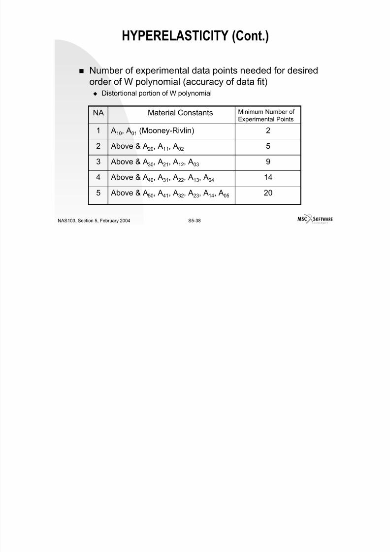
7/21/2019 Nonlinear Analysis Using MSC.nastran
http://slidepdf.com/reader/full/nonlinear-analysis-using-mscnastran 221/783
S5-37NAS103, Section 5, February 2004
Uniaxial tension/compression
Equibiaxial tension
Simple shear
Pure shear
Volumetric deformation Pure volumetric compaction
HYPERELASTICITY (Cont.)
Number of experimental data points needed for desiredorder of W polynomial (accuracy of data fit) Distortional portion of W polynomial
2A10, A01 (Mooney-Rivlin)1
Minimum Number ofExperimental Points
Material ConstantsNA
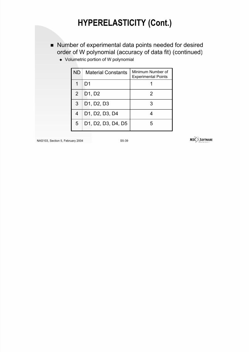
7/21/2019 Nonlinear Analysis Using MSC.nastran
http://slidepdf.com/reader/full/nonlinear-analysis-using-mscnastran 222/783
S5-38NAS103, Section 5, February 2004
20 Above & A50, A41, A32, A23, A14, A055
14 Above & A40, A31, A22, A13, A044
9 Above & A30, A21, A12, A0335 Above & A20, A11, A022
2 A10, A01 (Mooney Rivlin)1
HYPERELASTICITY (Cont.)
Number of experimental data points needed for desiredorder of W polynomial (accuracy of data fit) (continued) Volumetric portion of W polynomial
1D11
Minimum Number ofExperimental Points
Material ConstantsND

7/21/2019 Nonlinear Analysis Using MSC.nastran
http://slidepdf.com/reader/full/nonlinear-analysis-using-mscnastran 223/783
S5-39NAS103, Section 5, February 2004
5D1, D2, D3, D4, D55
4D1, D2, D3, D44
3D1, D2, D332D1, D22
1D11

7/21/2019 Nonlinear Analysis Using MSC.nastran
http://slidepdf.com/reader/full/nonlinear-analysis-using-mscnastran 224/783
User interface MATHP is used to supply or reference the material related data
Either the coefficients Aij and Di are to be specified, or data such asstress versus stretch is to be referenced
If experimental data is supplied, the value of the coefficients areestimated using least squares fitting of the data with polynomials
The coefficients are what is used by MSC.Nastran for the simulationof the constitutive properties
HYPERELASTICITY (Cont.)
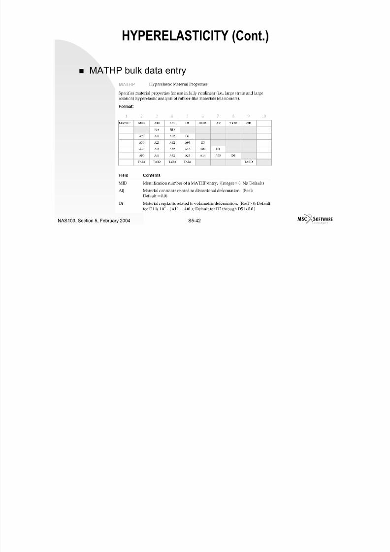
7/21/2019 Nonlinear Analysis Using MSC.nastran
http://slidepdf.com/reader/full/nonlinear-analysis-using-mscnastran 225/783
S5-41NAS103, Section 5, February 2004
p p
Τhe experimental stress versus stretch, etc. data is supplied using
TABLES1 entries
MATHP bulk data entry
HYPERELASTICITY (Cont.)

7/21/2019 Nonlinear Analysis Using MSC.nastran
http://slidepdf.com/reader/full/nonlinear-analysis-using-mscnastran 226/783
S5-42NAS103, Section 5, February 2004
MATHP bulk data entry (continued)
HYPERELASTICITY (Cont.)
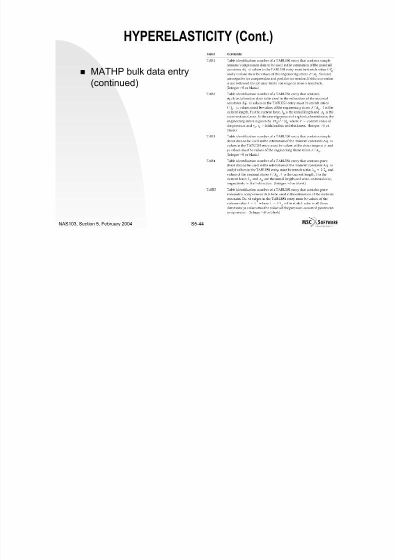
7/21/2019 Nonlinear Analysis Using MSC.nastran
http://slidepdf.com/reader/full/nonlinear-analysis-using-mscnastran 227/783
S5-43NAS103, Section 5, February 2004
MATHP bulk data entry(continued)
HYPERELASTICITY (Cont.)
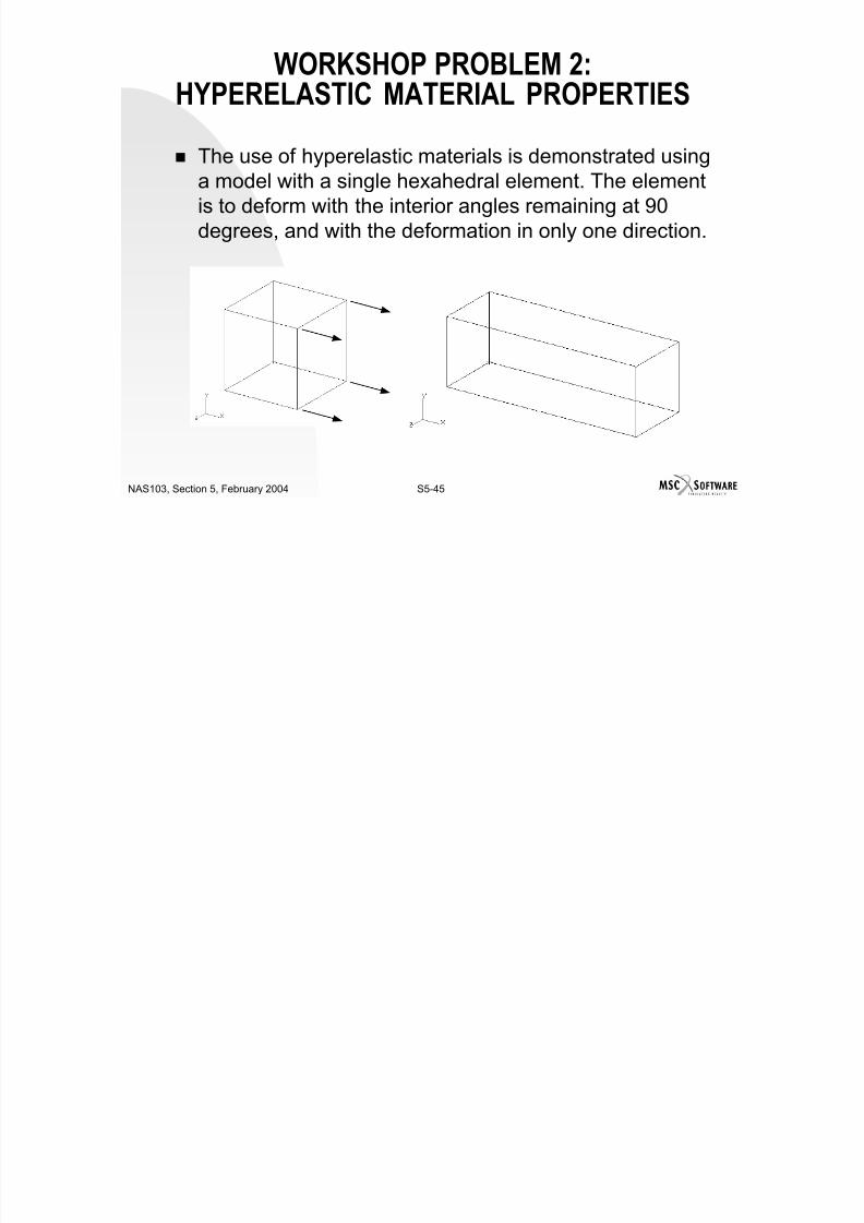
7/21/2019 Nonlinear Analysis Using MSC.nastran
http://slidepdf.com/reader/full/nonlinear-analysis-using-mscnastran 228/783
S5-44NAS103, Section 5, February 2004
WORKSHOP PROBLEM 2:HYPERELASTIC MATERIAL PROPERTIES
The use of hyperelastic materials is demonstrated usinga model with a single hexahedral element. The elementis to deform with the interior angles remaining at 90
degrees, and with the deformation in only one direction.

7/21/2019 Nonlinear Analysis Using MSC.nastran
http://slidepdf.com/reader/full/nonlinear-analysis-using-mscnastran 229/783
S5-45NAS103, Section 5, February 2004
WORKSHOP PROBLEM 2:HYPERELASTIC MATERIAL PROPERTIES
The needed information for the creation of the model is 1x1x1 single hexahedral element
Constrain the eight GRIDs to allow enforced motion in only the X-direction as follows Constrain one GRID’s all six D-of-Fs, e.g. GRID, 1, … ,123456 Constrain the other three GRID’s, of the element face containing the GRID
just constrained and normal to the X-direction, from motion in the X-direction, but allowing motion due to the Poisson effect

7/21/2019 Nonlinear Analysis Using MSC.nastran
http://slidepdf.com/reader/full/nonlinear-analysis-using-mscnastran 230/783
S5-46NAS103, Section 5, February 2004
Constrain the remaining four GRIDs like the first four GRIDs, but allowing
motion in the X-direction Using nine(9) MPCs constrain the hexahedral element to keep a
rectangular-box shape (all interior angles are 90 degrees), e.g.
-1.0171.016100MPC
-1.0171.013100MPC-1.0171.012100MPC
A2C2G2 A1C1G1SIDMPC
2
37
6
X1
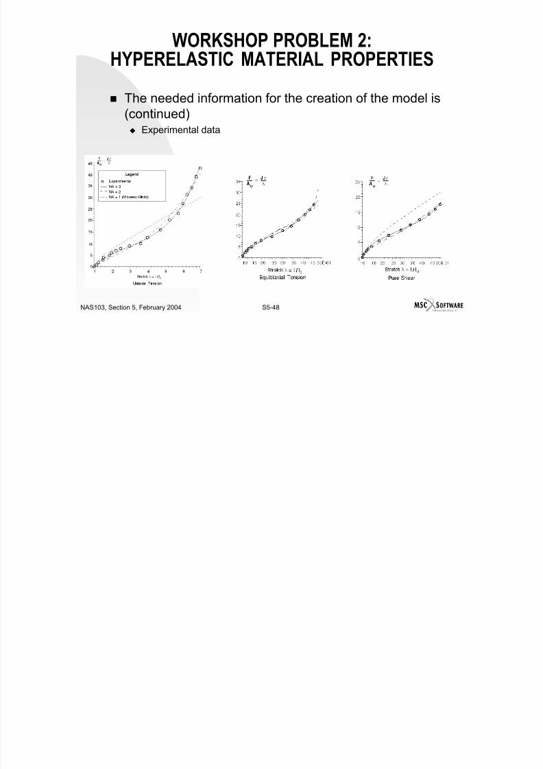
7/21/2019 Nonlinear Analysis Using MSC.nastran
http://slidepdf.com/reader/full/nonlinear-analysis-using-mscnastran 231/783
The needed information for the creation of the model is(continued) Experimental data
WORKSHOP PROBLEM 2:HYPERELASTIC MATERIAL PROPERTIES

7/21/2019 Nonlinear Analysis Using MSC.nastran
http://slidepdf.com/reader/full/nonlinear-analysis-using-mscnastran 232/783
S5-48NAS103, Section 5, February 2004
The needed information for the creation of the model is(continued) SOL 106
PARAM, LGDISP, 1
The bulk data entry NLPARM, and corresponding case control entry
WORKSHOP PROBLEM 2:HYPERELASTIC MATERIAL PROPERTIES
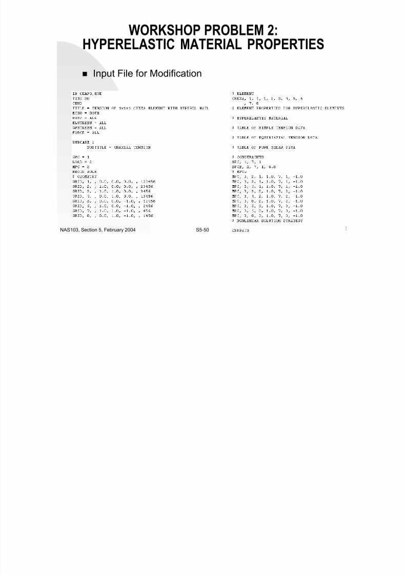
7/21/2019 Nonlinear Analysis Using MSC.nastran
http://slidepdf.com/reader/full/nonlinear-analysis-using-mscnastran 233/783
S5-49NAS103, Section 5, February 2004
WORKSHOP PROBLEM 2:HYPERELASTIC MATERIAL PROPERTIES
Input File for Modification
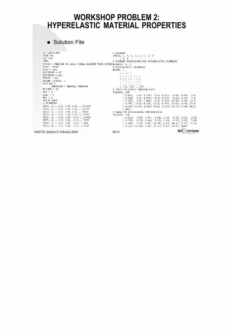
7/21/2019 Nonlinear Analysis Using MSC.nastran
http://slidepdf.com/reader/full/nonlinear-analysis-using-mscnastran 234/783
S5-50NAS103, Section 5, February 2004
WORKSHOP PROBLEM 2:HYPERELASTIC MATERIAL PROPERTIES
Solution File
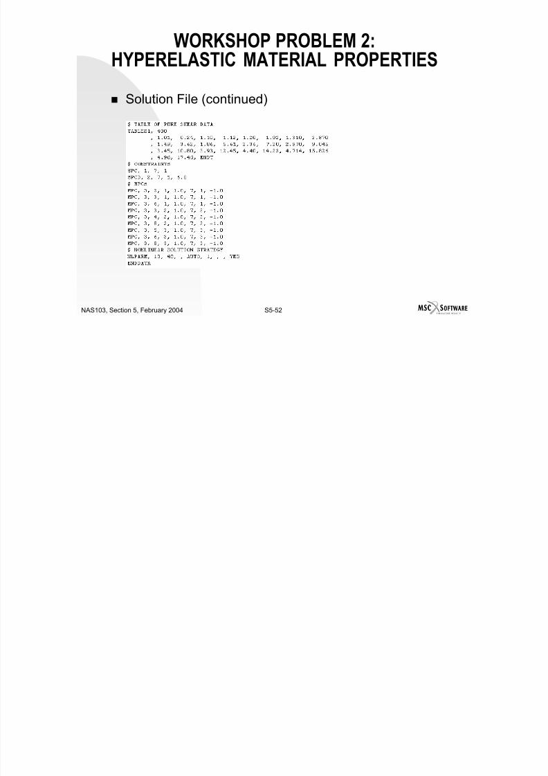
7/21/2019 Nonlinear Analysis Using MSC.nastran
http://slidepdf.com/reader/full/nonlinear-analysis-using-mscnastran 235/783
S5-51NAS103, Section 5, February 2004
WORKSHOP PROBLEM 2:HYPERELASTIC MATERIAL PROPERTIES
Solution File (continued)
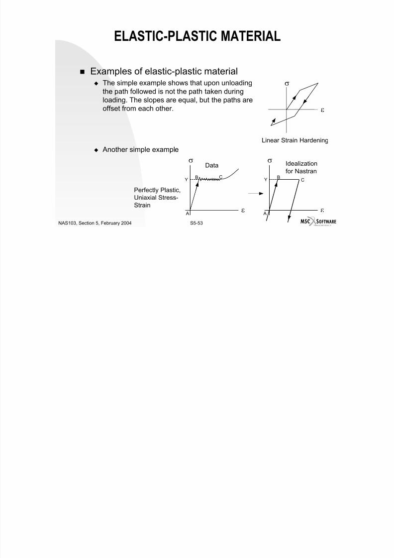
7/21/2019 Nonlinear Analysis Using MSC.nastran
http://slidepdf.com/reader/full/nonlinear-analysis-using-mscnastran 236/783
S5-52NAS103, Section 5, February 2004
ELASTIC-PLASTIC MATERIAL
Examples of elastic-plastic material The simple example shows that upon unloading
the path followed is not the path taken duringloading. The slopes are equal, but the paths are
offset from each other. ε
σ
Linear Strain Hardening

7/21/2019 Nonlinear Analysis Using MSC.nastran
http://slidepdf.com/reader/full/nonlinear-analysis-using-mscnastran 237/783
S5-53NAS103, Section 5, February 2004
Another simple example
g
ε
σ Idealizationfor Nastran
Y
A
BC
ε
σData
Y
A
B C
Perfectly Plastic,Uniaxial Stress-Strain
ELASTIC-PLASTIC MATERIAL (Cont.)
Modeling of material yielding Yield criterion
Defines the initiation of inelastic response of the material
A descriptive statement that defines conditions under which yielding will
begin yield function f(σij,Y)
σij is multi-axial stress state
Y is yield strength in uniaxial tension/compression
Yield criterion satisfied when f(σij,Y) = 0

7/21/2019 Nonlinear Analysis Using MSC.nastran
http://slidepdf.com/reader/full/nonlinear-analysis-using-mscnastran 238/783
S5-54NAS103, Section 5, February 2004
( ij )
If f(σij
,Y) < 0 the response is elastic
If f(σij,Y) > 0 the response is plastic
Example σe = function(σij) (effective stress, scalar)
f(σij,Y) = σe – Y
Note: there is a strain, εe, that corresponds to σe
ELASTIC-PLASTIC MATERIAL (Cont.)
Modeling of material yielding (continued) Hardening
The way the yield surface changes due to inelastic response Isotropic – yield surface expands uniformly
Kinematic – yield surface translates w/o distortion Combined – combination of isotropic and kinematic
Plastic flow direction Governs the plastic flow after yielding
Incremental stress versus incremental strain

7/21/2019 Nonlinear Analysis Using MSC.nastran
http://slidepdf.com/reader/full/nonlinear-analysis-using-mscnastran 239/783
S5-55NAS103, Section 5, February 2004
Incremental stress versus incremental strain Plasticity is path dependent There is not a unique relationship between stress and strain
There is a unique relationship between infinitesimal increments of stressand strain
ELASTIC-PLASTIC MATERIAL (Cont.)
Yield criterion Tresca (maximun shear stress)
Used to model metals with crystals having slip planes (resistance toshear force is relatively small), such as brittle and some ductile metals
Yielding begins when the maximum shear stress at a point equals themaximum shear stress at yield in uniaxial tension/compression
Yσσ 32 ±=−
Yσσ 13 ±=−

7/21/2019 Nonlinear Analysis Using MSC.nastran
http://slidepdf.com/reader/full/nonlinear-analysis-using-mscnastran 240/783
S5-56NAS103, Section 5, February 2004
where σi are the principal stresses
Yσσ 13 ±
Yσσ 21 ±=−
ELASTIC-PLASTIC MATERIAL (Cont.)
Yield criterion (continued) von Mises (distortional strain energy density)
Used to model metals with crystals having slip planes, such as ductilemetals
Yielding begins when the distortional strain energy density at a pointequals the distortional strain energy density at yield in uniaxialtension/compression
2222 Y1
])σ(σ)σ(σ)σ[(σ1
Y)f(σ ++

7/21/2019 Nonlinear Analysis Using MSC.nastran
http://slidepdf.com/reader/full/nonlinear-analysis-using-mscnastran 241/783
S5-57NAS103, Section 5, February 2004
133221ij Y
3
])σ(σ)σ(σ)σ[(σ
6
Y),f(σ −−+−+−=
ELASTIC-PLASTIC MATERIAL (Cont.)
Yield criterion (continued) Mohr-Coulomb
Used to model cohesive materials such as rock or concrete
Generalization of the Tresca criterion that includes the influence of
hydrostatic stress
where c and φ are coefficients for the cohesion and angle of internalfriction, respectively
2ccosφ)sinφσ(σσσY),f(σ 3131ij −++−=

7/21/2019 Nonlinear Analysis Using MSC.nastran
http://slidepdf.com/reader/full/nonlinear-analysis-using-mscnastran 242/783
S5-58NAS103, Section 5, February 2004
, p y
ELASTIC-PLASTIC MATERIAL (Cont.)
Yield criterion (continued) Drucker-Prager
Used to model cohesive materials such as sand or concrete
Generalization of von Mises criterion that includes the influence of
hydrostatic stress
where α and K are coefficients that are dependent on the cohesion andthe angle of internal friction
K JαIY),f(σ 21ij −+=

7/21/2019 Nonlinear Analysis Using MSC.nastran
http://slidepdf.com/reader/full/nonlinear-analysis-using-mscnastran 243/783
S5-59NAS103, Section 5, February 2004
g
ELASTIC-PLASTIC MATERIAL (Cont.)
Hardening, work Isotropic hardening
Yield surface becomes larger by expanding uniformly about the origin instress space; it retains its shape.
Effective plastic strain is used as the measure of hardening The effective strain, εe, is used as a measure of the size of the yield
surface
The Bauschinger effect is not taken into account

7/21/2019 Nonlinear Analysis Using MSC.nastran
http://slidepdf.com/reader/full/nonlinear-analysis-using-mscnastran 244/783
S5-60NAS103, Section 5, February 2004
ε2
ε3
Initial yield surface
Yield surface afterplastic deformation
O
Incremental loadingincreases size of surface
ε1
ELASTIC-PLASTIC MATERIAL (Cont.)
Hardening, work (continued) Kinematic hardening
Yield surface translates keeping its shape and size
Translate the yield surface in a direction normal to the yield surface
The location of the current center of the yield surface (o’) relative to theorigin of the principal strain coordinate system (o) is used as themeasure of hardening
The Bauschinger effect is accounted for
Physically reasonable results only for bilinear stress/strain relationship

7/21/2019 Nonlinear Analysis Using MSC.nastran
http://slidepdf.com/reader/full/nonlinear-analysis-using-mscnastran 245/783
S5-61NAS103, Section 5, February 2004
ε2
ε3
Initial yield surface
Yield surface afterplastic deformation
O
ε1
O’
ELASTIC-PLASTIC MATERIAL (Cont.)
Hardening, work (continued) Combined hardening
Combination of isotropic and kinematic hardening
The Bauschinger effect is accounted for
σa
σ

7/21/2019 Nonlinear Analysis Using MSC.nastran
http://slidepdf.com/reader/full/nonlinear-analysis-using-mscnastran 246/783
S5-62NAS103, Section 5, February 2004
σa
2σY
σa
σY
ε
Kinematic
Combined
Isotropic
ELASTIC-PLASTIC MATERIAL (Cont.)
Plastic flow direction MSC.Nastran uses associated flow rule to determine the plastic
flow direction
Uses plastic potential function equals the yield function
ε1 and σ1 axes coincide Plastic strain increment is calculated as follows
ij
P
ijσ
f λ dε
∂∂
=

7/21/2019 Nonlinear Analysis Using MSC.nastran
http://slidepdf.com/reader/full/nonlinear-analysis-using-mscnastran 247/783
S5-63NAS103, Section 5, February 2004
Where
Plastic strain increment is in direction normal to yield surface
ij
P
ijε is plastic strain
λ is a scalar factor used to relate incremental strains to finite stress
f is the yield function; f(σij,Y) = 0 is the yield surface.
ELASTIC-PLASTIC MATERIAL (Cont.)
Incremental stress versus incremental strain Plasticity is path dependent
There is not a unique relationship between stress and strain
There is a unique relationship between infinitesimal increments of
stress and strain For incremental stress/strain relationship the strain increment is
divided into an elastic and plastic increment
σ

7/21/2019 Nonlinear Analysis Using MSC.nastran
http://slidepdf.com/reader/full/nonlinear-analysis-using-mscnastran 248/783
S5-64NAS103, Section 5, February 2004
εP
ε
εEεP is the plastic strainεE is the elastic strain
ELASTIC-PLASTIC MATERIAL (Cont.)
Incremental stress versus incremental strain(continued) Relationship between differential increments of stress and plastic
strain
0dεε
f dσ
σ
f P
ijP
ij
ij
ij
=∂∂
+∂∂

7/21/2019 Nonlinear Analysis Using MSC.nastran
http://slidepdf.com/reader/full/nonlinear-analysis-using-mscnastran 249/783
S5-65NAS103, Section 5, February 2004

7/21/2019 Nonlinear Analysis Using MSC.nastran
http://slidepdf.com/reader/full/nonlinear-analysis-using-mscnastran 250/783
MATS1 bulk data entry
ELASTIC-PLASTIC MATERIAL (Cont.)

7/21/2019 Nonlinear Analysis Using MSC.nastran
http://slidepdf.com/reader/full/nonlinear-analysis-using-mscnastran 251/783
S5-67NAS103, Section 5, February 2004
MATS1 bulk data entry (continued)
ELASTIC-PLASTIC MATERIAL (Cont.)

7/21/2019 Nonlinear Analysis Using MSC.nastran
http://slidepdf.com/reader/full/nonlinear-analysis-using-mscnastran 252/783
S5-68NAS103, Section 5, February 2004
MATS1 bulk data entry (continued)
ELASTIC-PLASTIC MATERIAL (Cont.)

7/21/2019 Nonlinear Analysis Using MSC.nastran
http://slidepdf.com/reader/full/nonlinear-analysis-using-mscnastran 253/783
S5-69NAS103, Section 5, February 2004
MATS1 bulk data entry (continued)
ELASTIC-PLASTIC MATERIAL (Cont.)

7/21/2019 Nonlinear Analysis Using MSC.nastran
http://slidepdf.com/reader/full/nonlinear-analysis-using-mscnastran 254/783
S5-70NAS103, Section 5, February 2004
MATS1 bulk data entry(continued)
ELASTIC-PLASTIC MATERIAL (Cont.)
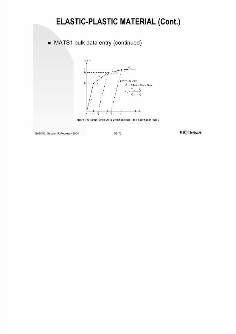
7/21/2019 Nonlinear Analysis Using MSC.nastran
http://slidepdf.com/reader/full/nonlinear-analysis-using-mscnastran 255/783
S5-71NAS103, Section 5, February 2004
MATS1 bulk data entry (continued)
ELASTIC-PLASTIC MATERIAL (Cont.)

7/21/2019 Nonlinear Analysis Using MSC.nastran
http://slidepdf.com/reader/full/nonlinear-analysis-using-mscnastran 256/783
S5-72NAS103, Section 5, February 2004
WORKSHOP PROBLEM 3: ELASTIC-PLASTIC MATERIAL PROPERTIES
The use of elastic-plastic material is demonstrated usinga model of a rectangular plate loaded in tension in onedirection.
X
Y
WP

7/21/2019 Nonlinear Analysis Using MSC.nastran
http://slidepdf.com/reader/full/nonlinear-analysis-using-mscnastran 257/783
S5-73NAS103, Section 5, February 2004
L
T = plate thickness
WORKSHOP PROBLEM 3: ELASTIC-PLASTIC MATERIAL PROPERTIES
3 0 6E ( i)
0.1T (in.)
10.0W (in.)
50.0L (in.)
ValuePara-meter
Elastic-plastic model von Mises yield criterion
Isotropic hardening
950 0
1000.0
800.0
AppliedLoad, P
(lbf)

7/21/2019 Nonlinear Analysis Using MSC.nastran
http://slidepdf.com/reader/full/nonlinear-analysis-using-mscnastran 258/783
S5-74NAS103, Section 5, February 2004
850.0σY (psi)
3.0e+4ET (psi)
0.25ν3.0e+6E (psi)
0.0
950.0
WORKSHOP PROBLEM 3: ELASTIC-PLASTIC MATERIAL PROPERTIES
Include in model SOL 106
Two subcases for loading, and two subcases for unloading, e.g. SUBCASE 2
SUBTITLE = PLASTIC LOAD TO 1000 lbf LOAD = 2
NLPARM = 2
Use 1, 8, 5, and 2 increments for the NLPARM bulk data entries, for thefour subcases, e.g.
Case control
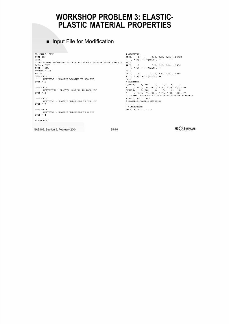
7/21/2019 Nonlinear Analysis Using MSC.nastran
http://slidepdf.com/reader/full/nonlinear-analysis-using-mscnastran 259/783
S5-75NAS103, Section 5, February 2004
Case control SUBCASE 2
NLPARM = 2
Bulk data NLPARM, 2, 8,, AUTO,,,P

7/21/2019 Nonlinear Analysis Using MSC.nastran
http://slidepdf.com/reader/full/nonlinear-analysis-using-mscnastran 260/783
WORKSHOP PROBLEM 3: ELASTIC-PLASTIC MATERIAL PROPERTIES
Input File for Modification (continued)
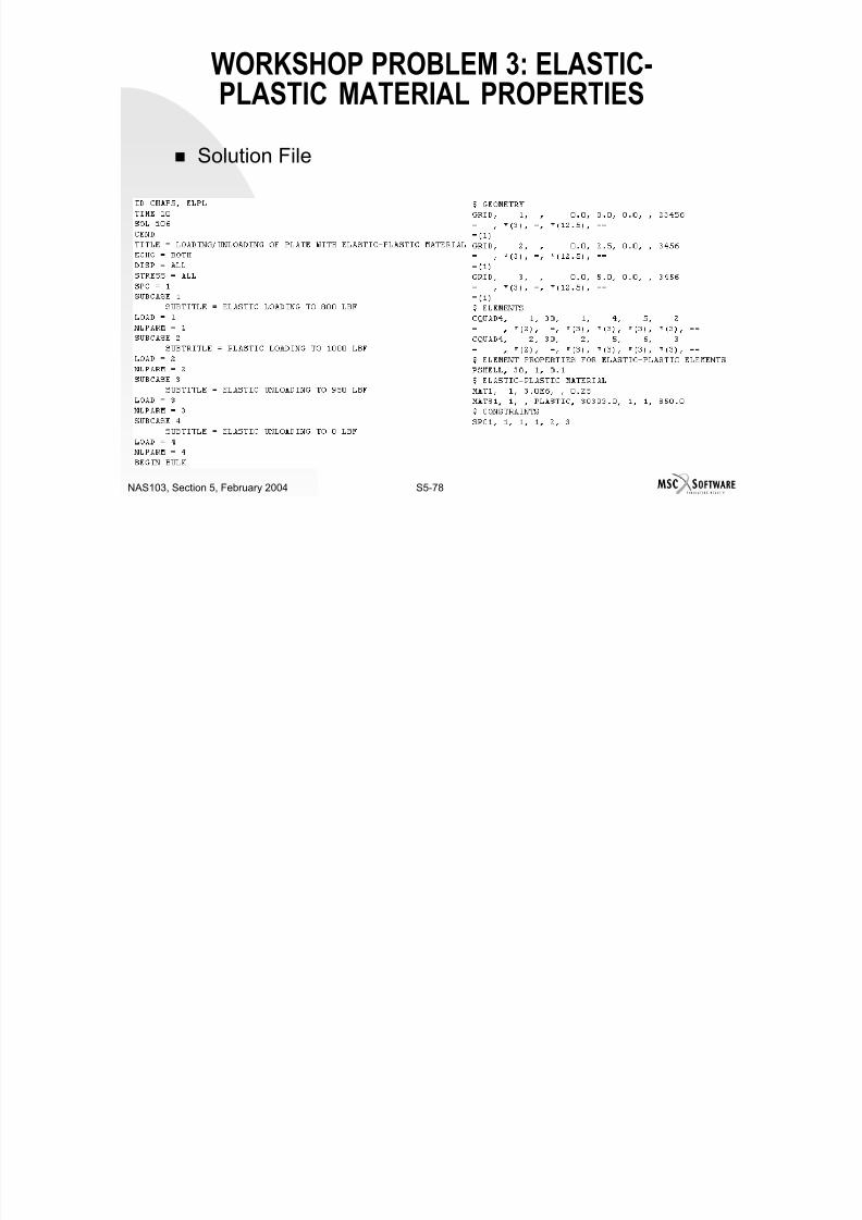
7/21/2019 Nonlinear Analysis Using MSC.nastran
http://slidepdf.com/reader/full/nonlinear-analysis-using-mscnastran 261/783
S5-77NAS103, Section 5, February 2004
WORKSHOP PROBLEM 3: ELASTIC-PLASTIC MATERIAL PROPERTIES
Solution File

7/21/2019 Nonlinear Analysis Using MSC.nastran
http://slidepdf.com/reader/full/nonlinear-analysis-using-mscnastran 262/783
S5-78NAS103, Section 5, February 2004
WORKSHOP PROBLEM 3: ELASTIC-PLASTIC MATERIAL PROPERTIES
Solution File (continued)

7/21/2019 Nonlinear Analysis Using MSC.nastran
http://slidepdf.com/reader/full/nonlinear-analysis-using-mscnastran 263/783
S5-79NAS103, Section 5, February 2004
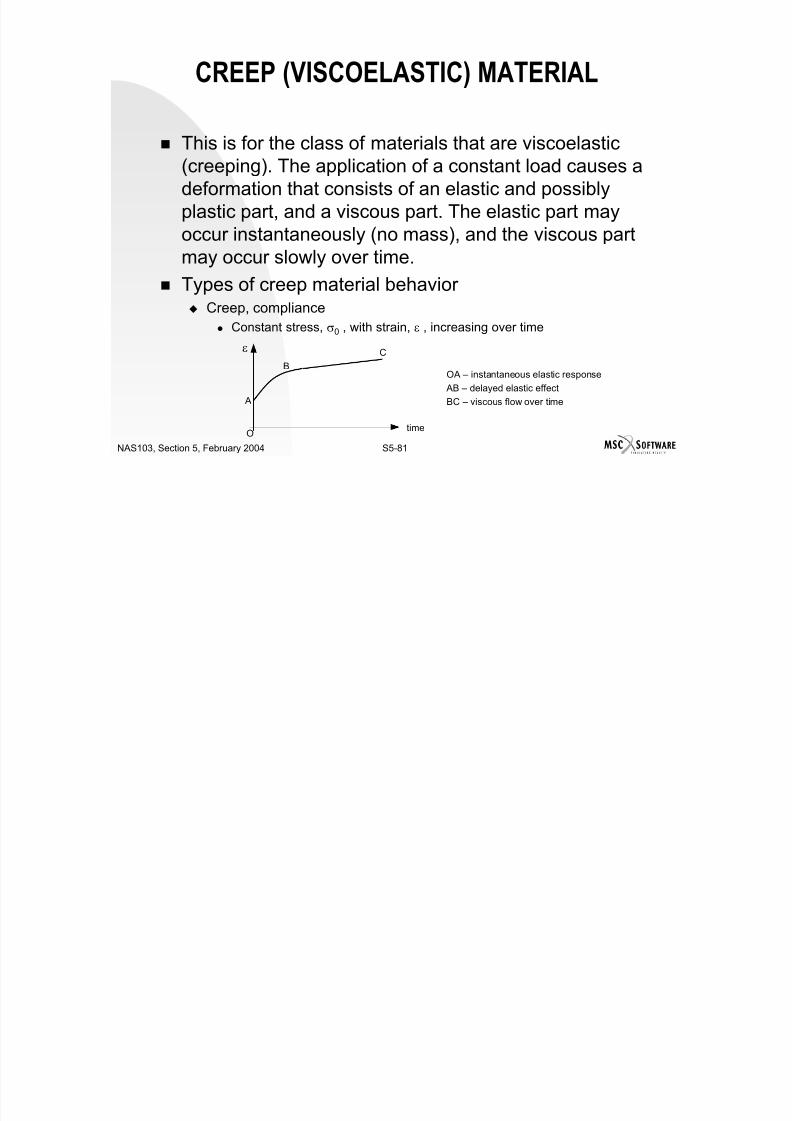
7/21/2019 Nonlinear Analysis Using MSC.nastran
http://slidepdf.com/reader/full/nonlinear-analysis-using-mscnastran 264/783
S5-80NAS103, Section 5, February 2004
CREEP (VISCOELASTIC) MATERIAL
This is for the class of materials that are viscoelastic(creeping). The application of a constant load causes adeformation that consists of an elastic and possiblyplastic part, and a viscous part. The elastic part mayoccur instantaneously (no mass), and the viscous partmay occur slowly over time.
Types of creep material behavior
Creep complianceC t t t ith t i i i ti

7/21/2019 Nonlinear Analysis Using MSC.nastran
http://slidepdf.com/reader/full/nonlinear-analysis-using-mscnastran 265/783
S5-81NAS103, Section 5, February 2004
Creep, compliance Constant stress, σ0 , with strain, ε , increasing over time
O
A
B
C
time
ε
OA – instantaneous elastic response
AB – delayed elastic effect
BC – viscous flow over time
CREEP (VISCOELASTIC) MATERIAL(Cont.)
Types of creep material behavior (continued) Creep, compliance (continued)
Creep, three stage, with constant stress, σ0
Otime
ε
e
p
P i S d T ti
lr
r
er
sc
p
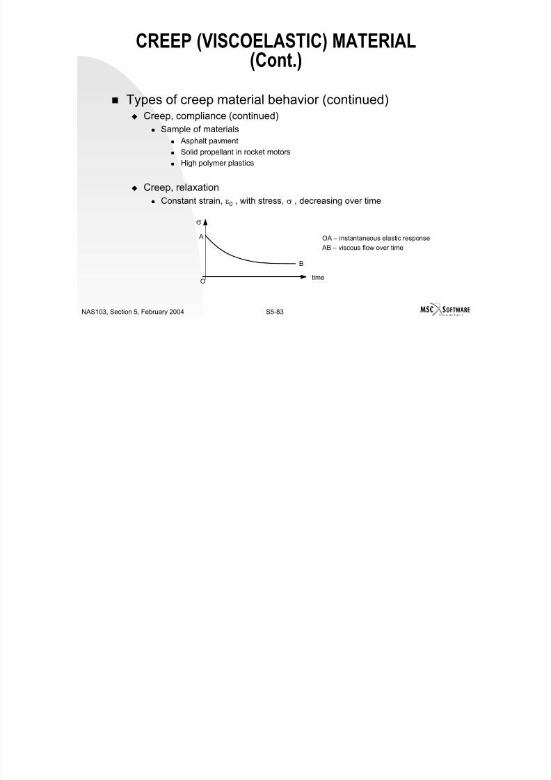
7/21/2019 Nonlinear Analysis Using MSC.nastran
http://slidepdf.com/reader/full/nonlinear-analysis-using-mscnastran 266/783
S5-82NAS103, Section 5, February 2004
e – elastic deformation lr – load removed, then
p – plastic deformation different path
Primary – deformation rate decreases with time er – elastic recovery
Secondary – constant minimum creep rate r – ruptureTertiary – rapid increase of creep rate sc – secondary creep
Primary Secondary Tertiary
CREEP (VISCOELASTIC) MATERIAL(Cont.)
Types of creep material behavior (continued) Creep, compliance (continued)
Sample of materials Asphalt pavment
Solid propellant in rocket motors
High polymer plastics
Creep, relaxation Constant strain, ε0 , with stress, σ , decreasing over time
σ

7/21/2019 Nonlinear Analysis Using MSC.nastran
http://slidepdf.com/reader/full/nonlinear-analysis-using-mscnastran 267/783
S5-83NAS103, Section 5, February 2004
O time
A
B
OA – instantaneous elastic response
AB – viscous flow over time
CREEP (VISCOELASTIC) MATERIAL(Cont.)
Types of creep material behavior (continued) Creep, relaxation (continued)
Sample of materials Prestress tendons in prestressed concrete
Prestress bolts at high temperatures that clamp rigid flanges of a machine
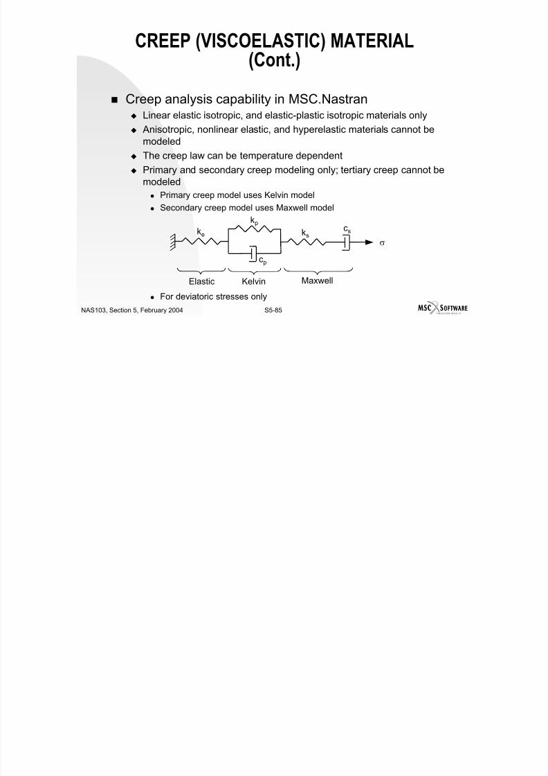
7/21/2019 Nonlinear Analysis Using MSC.nastran
http://slidepdf.com/reader/full/nonlinear-analysis-using-mscnastran 268/783
S5-84NAS103, Section 5, February 2004
CREEP (VISCOELASTIC) MATERIAL(Cont.)
Creep analysis capability in MSC.Nastran Linear elastic isotropic, and elastic-plastic isotropic materials only
Anisotropic, nonlinear elastic, and hyperelastic materials cannot bemodeled
The creep law can be temperature dependent Primary and secondary creep modeling only; tertiary creep cannot be
modeled Primary creep model uses Kelvin model
Secondary creep model uses Maxwell model
kpc

7/21/2019 Nonlinear Analysis Using MSC.nastran
http://slidepdf.com/reader/full/nonlinear-analysis-using-mscnastran 269/783
S5-85NAS103, Section 5, February 2004
For deviatoric stresses only
ke kscs
cp
σ
Kelvin MaxwellElastic
User interface MAT1 used to specify E, G, ν, ρ
CREEP is used to specify T0, Kp, Cp, Cs, TABLES1, etc.
TABLES1 is used to specify the creep
ΜΑΤS1 is used if there is plastic deformation
CREEP (VISCOELASTIC) MATERIAL(Cont.)

7/21/2019 Nonlinear Analysis Using MSC.nastran
http://slidepdf.com/reader/full/nonlinear-analysis-using-mscnastran 270/783
S5-86NAS103, Section 5, February 2004
CREEP bulk data entry
CREEP (VISCOELASTIC) MATERIAL(Cont.)

7/21/2019 Nonlinear Analysis Using MSC.nastran
http://slidepdf.com/reader/full/nonlinear-analysis-using-mscnastran 271/783
S5-87NAS103, Section 5, February 2004

7/21/2019 Nonlinear Analysis Using MSC.nastran
http://slidepdf.com/reader/full/nonlinear-analysis-using-mscnastran 272/783
CREEP bulk data entry (continued)
CREEP (VISCOELASTIC) MATERIAL(Cont.)

7/21/2019 Nonlinear Analysis Using MSC.nastran
http://slidepdf.com/reader/full/nonlinear-analysis-using-mscnastran 273/783
S5-89NAS103, Section 5, February 2004

7/21/2019 Nonlinear Analysis Using MSC.nastran
http://slidepdf.com/reader/full/nonlinear-analysis-using-mscnastran 274/783
CREEP bulk data entry (continued)
CREEP (VISCOELASTIC) MATERIAL(Cont.)

7/21/2019 Nonlinear Analysis Using MSC.nastran
http://slidepdf.com/reader/full/nonlinear-analysis-using-mscnastran 275/783
S5-91NAS103, Section 5, February 2004
CREEP bulk data entry (continued)
CREEP (VISCOELASTIC) MATERIAL(Cont.)

7/21/2019 Nonlinear Analysis Using MSC.nastran
http://slidepdf.com/reader/full/nonlinear-analysis-using-mscnastran 276/783
S5-92NAS103, Section 5, February 2004
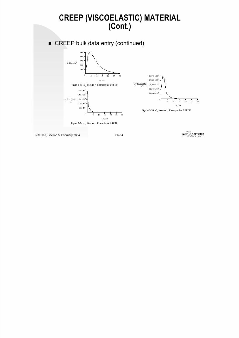
7/21/2019 Nonlinear Analysis Using MSC.nastran
http://slidepdf.com/reader/full/nonlinear-analysis-using-mscnastran 277/783
CREEP bulk data entry (continued)
CREEP (VISCOELASTIC) MATERIAL(Cont.)

7/21/2019 Nonlinear Analysis Using MSC.nastran
http://slidepdf.com/reader/full/nonlinear-analysis-using-mscnastran 278/783
S5-94NAS103, Section 5, February 2004
CREEP bulk data entry (continued)
CREEP (VISCOELASTIC) MATERIAL(Cont.)

7/21/2019 Nonlinear Analysis Using MSC.nastran
http://slidepdf.com/reader/full/nonlinear-analysis-using-mscnastran 279/783
S5-95NAS103, Section 5, February 2004
WORKSHOP PROBLEM 4: CREEPMATERIAL PROPERTIES
Calculate the creep strain in a cylindrical bar that issubjected to axial step loads/stresses.
Cross-sectionalarea = 1.0
E = 21.8e+6
ν = 0.32
CROD
All DOFfixed
Only DOF indirection of
force is free
Force
10.0 in
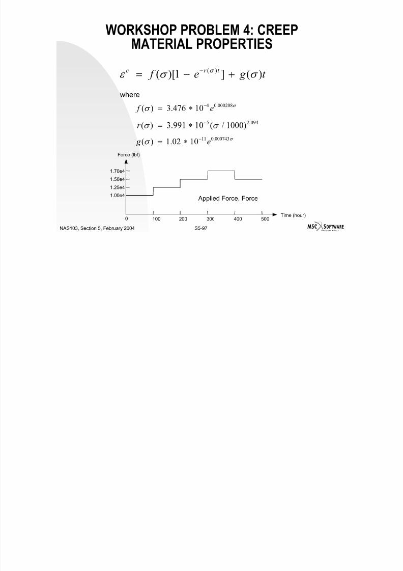
7/21/2019 Nonlinear Analysis Using MSC.nastran
http://slidepdf.com/reader/full/nonlinear-analysis-using-mscnastran 280/783
S5-96NAS103, Section 5, February 2004
WORKSHOP PROBLEM 4: CREEPMATERIAL PROPERTIES
t g e f t r c )(]1)[( )( σ σ ε σ +−= −
σ σ 000208.0410476.3)( e f −∗=
094.25 )1000/(10991.3)( σ σ −∗=r
σ σ 000743.0111002.1)( e g −∗=
where
1.70e4
Force (lbf)

7/21/2019 Nonlinear Analysis Using MSC.nastran
http://slidepdf.com/reader/full/nonlinear-analysis-using-mscnastran 281/783
S5-97NAS103, Section 5, February 2004
0 100 200 300 400 500
1.00e4
1.25e4
1.50e4
Time (hour)
Applied Force, Force
WORKSHOP PROBLEM 4: CREEPMATERIAL PROPERTIES
Include in model SOL 106
Five subcase pairs (total of 10 subcases), with the first subcase in apair for elastic loading and the second subcase in the pair for creeploading, e.g. SUBCASE 2O
SUBTITLE = ELASTIC
LOAD = 2 $ load = 1.25e4
NLPARM = 10 $ control of elastic solution
SUBCASE 21 SUBTITLE = CREEP

7/21/2019 Nonlinear Analysis Using MSC.nastran
http://slidepdf.com/reader/full/nonlinear-analysis-using-mscnastran 282/783
S5-98NAS103, Section 5, February 2004
LOAD = 2 $ load = 1.25e4
NLPARM = 20 $ control of creep solution
WORKSHOP PROBLEM 4: CREEPMATERIAL PROPERTIES
Include in model (continued) For the bulk data it is necessary to specify the loading over time,
definition of the creep model, control of the elastic solution, and controlof the creep solution, e.g. FORCE, 2, 2, , 1.25E4, 1.0, 0.0, 0.0
CREEP, 1, … FORM = CRLAW
TYPE = 222
NLPARM, 10, 1
NLPARM, 20, 5, 20, , , , , YES Note: total creep time = NINC * DT

7/21/2019 Nonlinear Analysis Using MSC.nastran
http://slidepdf.com/reader/full/nonlinear-analysis-using-mscnastran 283/783
S5-99NAS103, Section 5, February 2004
WORKSHOP PROBLEM 4: CREEPMATERIAL PROPERTIES
Input File for Modification

7/21/2019 Nonlinear Analysis Using MSC.nastran
http://slidepdf.com/reader/full/nonlinear-analysis-using-mscnastran 284/783
S5-100NAS103, Section 5, February 2004
WORKSHOP PROBLEM 4: CREEPMATERIAL PROPERTIES
Input File for Modification (continued)

7/21/2019 Nonlinear Analysis Using MSC.nastran
http://slidepdf.com/reader/full/nonlinear-analysis-using-mscnastran 285/783
S5-101NAS103, Section 5, February 2004
WORKSHOP PROBLEM 4: CREEPMATERIAL PROPERTIES
Solution File

7/21/2019 Nonlinear Analysis Using MSC.nastran
http://slidepdf.com/reader/full/nonlinear-analysis-using-mscnastran 286/783
S5-102NAS103, Section 5, February 2004
WORKSHOP PROBLEM 4: CREEPMATERIAL PROPERTIES
Solution File (continued)

7/21/2019 Nonlinear Analysis Using MSC.nastran
http://slidepdf.com/reader/full/nonlinear-analysis-using-mscnastran 287/783
S5-103NAS103, Section 5, February 2004
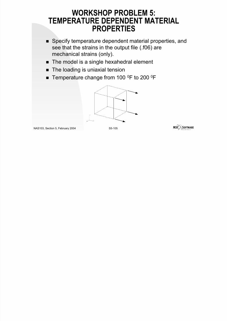
7/21/2019 Nonlinear Analysis Using MSC.nastran
http://slidepdf.com/reader/full/nonlinear-analysis-using-mscnastran 288/783
S5-104NAS103, Section 5, February 2004
WORKSHOP PROBLEM 5:TEMPERATURE DEPENDENT MATERIAL
PROPERTIES
Specify temperature dependent material properties, andsee that the strains in the output file (.f06) aremechanical strains (only).
The model is a single hexahedral element
The loading is uniaxial tension
Temperature change from 100 0F to 200 0F

7/21/2019 Nonlinear Analysis Using MSC.nastran
http://slidepdf.com/reader/full/nonlinear-analysis-using-mscnastran 289/783
S5-105NAS103, Section 5, February 2004
The needed information for the creation of the model is 1x1x1 single hexahedral element; units are inch.
Constrain the eight GRIDs to allow enforced motion in only the X-direction as follows Constrain the four GRID’s, in the plane X=0 (Y-Z plane), all six D-of-Fs, e.g.
GRID, 1, … ,123456
Constrain the other four GRID’s, in the plane X=1, D-of-Fs 3456, e.g.GRID, 2, …, 3456
Elastic modulus, E, is 8.0e6, 100 0F ; and 4.0e6, 200 0F.
Poisson’s ratio, ν, is 0.3 at all temperatures Thermal expansion coefficient is 1.0e-5 at all temperatures
Applied load is 10 000 lbf
WORKSHOP PROBLEM 5:TEMPERATURE DEPENDENT MATERIAL
PROPERTIES

7/21/2019 Nonlinear Analysis Using MSC.nastran
http://slidepdf.com/reader/full/nonlinear-analysis-using-mscnastran 290/783
S5-106NAS103, Section 5, February 2004
Applied load is 10,000 lbf
Initial and final temperature is 100 0F and 200 0F, respectively
The model has zero stress at the initial temperature
WORKSHOP PROBLEM 5:TEMPERATURE DEPENDENT MATERIAL
PROPERTIES
The needed information for the creation of the model is(continued) SOL 106
The case control section is used to select the initial temperature,
followed by two subcases, the latter of which is used to select the finaltemperature Case control
TEMP (INIT) = 10
SUBCASE 1
LOAD = 1 NLPARM = 1
SUBCASE 2

7/21/2019 Nonlinear Analysis Using MSC.nastran
http://slidepdf.com/reader/full/nonlinear-analysis-using-mscnastran 291/783
S5-107NAS103, Section 5, February 2004
LOAD = 1
NLPARM = 2
TEMP (LOAD) = 20
The needed information for the creation of the model is(continued) The bulk data section is used to specify the initial and final temperature,
and the control of the nonlinear process Bulk data
$ INITIAL TEMPERATURE DISTRIBUTION
TEMPD, 10, 100.0
$ FINAL TEMPERATURE DISTRIBUTION
TEMPD, 20, 200.0
NLPARM, 1, 1
NLPARM, 2, 5
WORKSHOP PROBLEM 5:TEMPERATURE DEPENDENT MATERIAL
PROPERTIES

7/21/2019 Nonlinear Analysis Using MSC.nastran
http://slidepdf.com/reader/full/nonlinear-analysis-using-mscnastran 292/783
S5-108NAS103, Section 5, February 2004
WORKSHOP PROBLEM 5:TEMPERATURE DEPENDENT MATERIAL
PROPERTIES
Nastran input file, with entries to be included
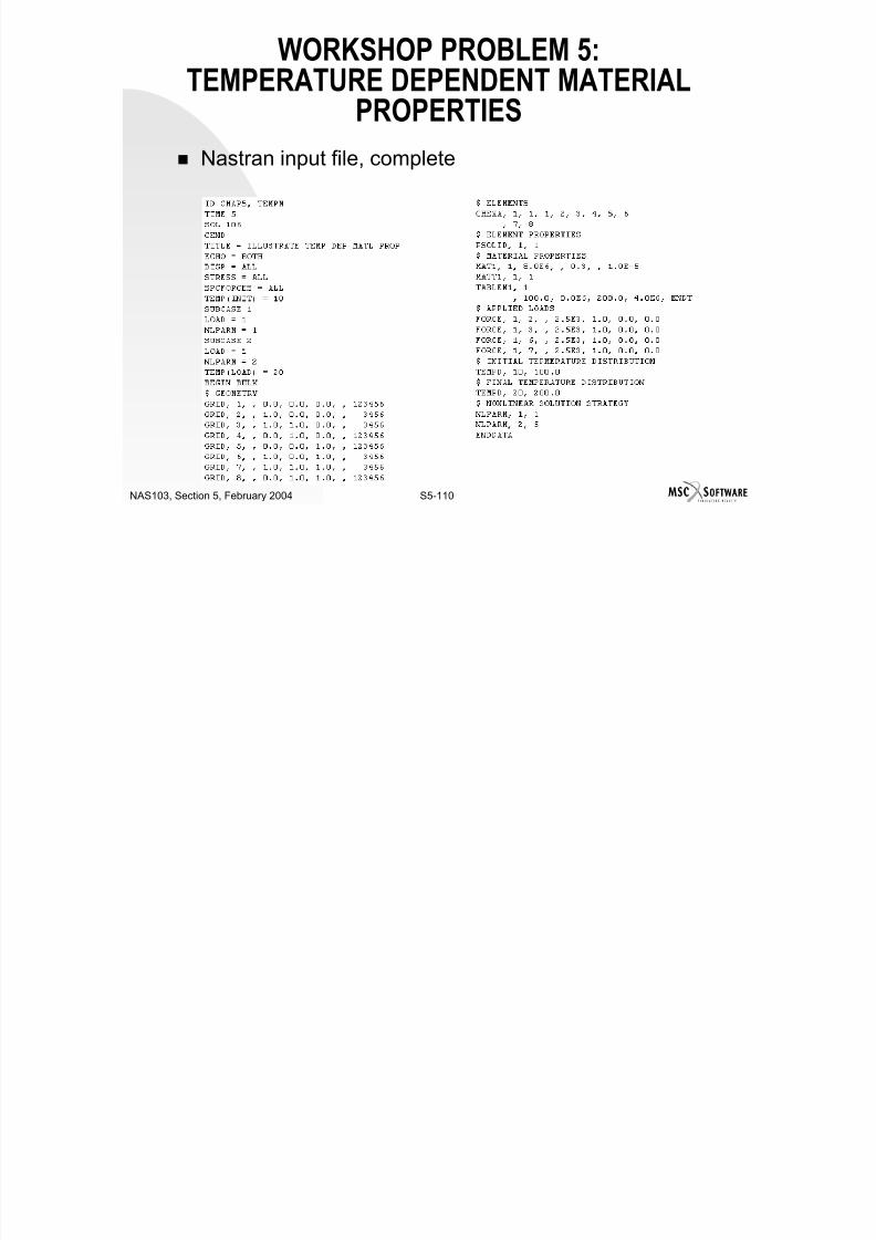
7/21/2019 Nonlinear Analysis Using MSC.nastran
http://slidepdf.com/reader/full/nonlinear-analysis-using-mscnastran 293/783
S5-109NAS103, Section 5, February 2004
WORKSHOP PROBLEM 5:TEMPERATURE DEPENDENT MATERIAL
PROPERTIES
Nastran input file, complete

7/21/2019 Nonlinear Analysis Using MSC.nastran
http://slidepdf.com/reader/full/nonlinear-analysis-using-mscnastran 294/783
S5-110NAS103, Section 5, February 2004
WORKSHOP PROBLEM 6: ELASTIC-PERFECTLY PLASTIC MATERIAL
PROPERTIES
Model is seven member truss, constrained from out ofplane motion
Use CROD elements
Material is elastic-perfectly plastic
Apply (enforced) displacements
Compute limit load for structure
2h
δ δ
σy1 σy1
σy2
σy2
σy22h = 10.0
A = 1.0
F = all 6 DOF fixed
ET
= 0.0
σy1 = 100.0
σy2 = 300.0

7/21/2019 Nonlinear Analysis Using MSC.nastran
http://slidepdf.com/reader/full/nonlinear-analysis-using-mscnastran 295/783
S5-111NAS103, Section 5, February 2004
2h
σy2σy2
F F
E = 2.0e5y2
δ = 0.05
WORKSHOP PROBLEM 6: ELASTIC-PERFECTLY PLASTIC MATERIAL
PROPERTIES
Include in model SOL 106
Case control NLPARM = 1
Bulk data Two entries for elastic-perfectly plastic properties
NLPARM, 1, 20, , , , , ,YES

7/21/2019 Nonlinear Analysis Using MSC.nastran
http://slidepdf.com/reader/full/nonlinear-analysis-using-mscnastran 296/783
S5-112NAS103, Section 5, February 2004
WORKSHOP PROBLEM 6: ELASTIC-PERFECTLY PLASTIC MATERIAL
PROPERTIES
Input File for Modification

7/21/2019 Nonlinear Analysis Using MSC.nastran
http://slidepdf.com/reader/full/nonlinear-analysis-using-mscnastran 297/783
S5-113NAS103, Section 5, February 2004
WORKSHOP PROBLEM 6: ELASTIC-PERFECTLY PLASTIC MATERIAL
PROPERTIES
Solution File

7/21/2019 Nonlinear Analysis Using MSC.nastran
http://slidepdf.com/reader/full/nonlinear-analysis-using-mscnastran 298/783
S5-114NAS103, Section 5, February 2004
SECTION 6
NONLINEAR ELEMENTS

7/21/2019 Nonlinear Analysis Using MSC.nastran
http://slidepdf.com/reader/full/nonlinear-analysis-using-mscnastran 299/783
S6-1NAS 103, Section 6, December 2003
7/21/2019 Nonlinear Analysis Using MSC.nastran
http://slidepdf.com/reader/full/nonlinear-analysis-using-mscnastran 300/783
S6-2NAS 103, Section 6, December 2003
TABLE OF CONTENTS
Page
Types Of Nonlinear Elements 6-6Small Versus Large Strain 6-7
Small Strain Elements 6-10
Corotational Formulation 6-14
One-dimensional Small Strain Element Library 6-16Rod, Conrod, Tube (Small Strain) 6-17
Beam (Small Strain) 6-20
Two-dimensional Small Strain Element Library 6-30
Nonlinear Shell And Plate Elements 6-31
Output For Shell And Plate Elements 6-36
Three-dimensional Small Strain Element Library 6-38
7/21/2019 Nonlinear Analysis Using MSC.nastran
http://slidepdf.com/reader/full/nonlinear-analysis-using-mscnastran 301/783
S6-3NAS 103, Section 6, December 2003
Solid Elements 6-39
Large Strain Elements 6-43
Hyperelastic Elements 6-44
TABLE OF CONTENTS
Page
Total Lagrangian Formulation 6-47Volumetric Locking 6-49
Output For Hyperelastic Elements 6-51
Hyperelastic Element Limitations 6-54
Planar Hyperelastic Elements 6-55Solid Hyperelastic Elements 6-60
Contact (Interface) Elements 6-64
Gap Element 6-65
3-D Slideline Contact 6-80
BCONP Bulk Data Entry 6-89
BLSEG Bulk Data Entry 6-92
BFRIC B lk D t E t 6 95

7/21/2019 Nonlinear Analysis Using MSC.nastran
http://slidepdf.com/reader/full/nonlinear-analysis-using-mscnastran 302/783
S6-4NAS 103, Section 6, December 2003
BFRIC Bulk Data Entry 6-95
BWIDTH Bulk Data Entry 6-96
BOUTPUT Bulk Data Entry 6-99
TABLE OF CONTENTS
Page
BOUTPUT Case Control Command 6-100PARAM ADPCON 6-102
Summary 6-103
Large Strain (Hyperelastic) Physical Elements 6-109
Example Problem One 6-117Example Problem Two 6-122
Example Problem Three 6-124
Workshop Problem One 6-127
Solution To Workshop Problem One 6-130

7/21/2019 Nonlinear Analysis Using MSC.nastran
http://slidepdf.com/reader/full/nonlinear-analysis-using-mscnastran 303/783
S6-5NAS 103, Section 6, December 2003
TYPES OF NONLINEAR ELEMENTS
Physical elements Small strain (ROD, BEAM, QUAD4, TRIA3, HEXA, PENTA, TETRA). Large strain (QUAD4, QUAD8, QUAD, QUADX, TRIA3, TRIA6, TRIAX,
HEXA, PENTA, TETRA).
Contact (interface) elements GAP 3-D slideline.

7/21/2019 Nonlinear Analysis Using MSC.nastran
http://slidepdf.com/reader/full/nonlinear-analysis-using-mscnastran 304/783
S6-6NAS 103, Section 6, December 2003
SMALL VERSUS LARGE STRAIN
Longitudinal strain:
Shear strain:
Small strain does not include the quadratic terms in thesquare brackets
εx δuδx------ 1
2--- δu
δx------ 2 δv
δx------ 2 δw
δx------- 2+ ++=
εyδv
δy------
1
2---
δu
δy------
2 δv
δy------
2 δw
δy-------
2
+ ++=
+ [y
w
x
w
y
v
x
v
y
u
x
u
x
v
y
u xy
]

7/21/2019 Nonlinear Analysis Using MSC.nastran
http://slidepdf.com/reader/full/nonlinear-analysis-using-mscnastran 305/783
S6-7NAS 103, Section 6, December 2003
square brackets.
SMALL VERSUS LARGE STRAIN
Large strain-displacement matrix (B) is nonlinear.
For large strains, different definitions of stress and strainare available.
Must use conjugate stress-strain definition.
All strain definitions give the same result for small strains(<10%).
Small (infinitesimal) strain:
Large (logarithmic) strain:
ε ∆ l
l 0
-----=
ε l d
l ---- ln
l
l 0
----=∫=

7/21/2019 Nonlinear Analysis Using MSC.nastran
http://slidepdf.com/reader/full/nonlinear-analysis-using-mscnastran 306/783
S6-8NAS 103, Section 6, December 2003
ε n 1 ε+( ) ε or ε 1≅= <<
SMALL VERSUS LARGE STRAIN
At 10% stretch
Acceptable for engineering accuracy with a discrepancyof 0.47%.
At 100% stretchNot acceptable for engineering accuracy.
In metal forming problems, stretch could be more than100%, and large strain capability is required.
In most structural problems, small strain is adequate.
Large strain (> 10%) may be acceptable if it is highlylocalized, i.e., small compared to the total strain energy.
ε 0.1=( ) : ε ln 1.1 0.0953==
ε 1.0=( ) : ε ln 2 0.693==

7/21/2019 Nonlinear Analysis Using MSC.nastran
http://slidepdf.com/reader/full/nonlinear-analysis-using-mscnastran 307/783
S6-9NAS 103, Section 6, December 2003
SMALL STRAIN ELEMENTS
General May have large displacements and rotations (geometric nonlinear). May have nonlinear material constitutive relationship.
Elastic (isotropic, orthotropic, anisotropic)
Nonlinear elastic (isotropic, anisotropic)
Elastic-plastic (isotropic, anisotropic)
Temperature-dependent (Elastic: isotropic, orthotropic, anisotropic;Nonlinear elastic: isotropic)
Creep
Equilibrium is satisfied in deformed configuration.
Based on corotational formulation - A set of corotational axes thatcontinuously rotates with the element.
Use engineering strain, which is the strain in the element once theelement is rigidly rotated back to its original position
7/21/2019 Nonlinear Analysis Using MSC.nastran
http://slidepdf.com/reader/full/nonlinear-analysis-using-mscnastran 308/783
S6-10NAS 103, Section 6, December 2003
element is rigidly rotated back to its original position.
SMALL STRAIN ELEMENTS
Displacement of an element is split into: Rigid body motion Element net deformation
Good for large global displacements and large globalrotations with small element strains.
Converges faster with fine meshes than in coarsemeshes.
Stiffness matrix is divided into material and geometric
parts. Geometric part is included by PARAM,LGDISP.
Nonlinear material is included by MATS1 MATTi (1 2

7/21/2019 Nonlinear Analysis Using MSC.nastran
http://slidepdf.com/reader/full/nonlinear-analysis-using-mscnastran 309/783
S6-11NAS 103, Section 6, December 2003
Nonlinear material is included by MATS1, MATTi (1, 2,
9), or CREEP.
SMALL STRAIN ELEMENTS
Two types of OUTPUT FORMAT: NONLINEAR - STRESS in subcase LINEAR - FORCE in subcase
Strains in linear solution sequences are total strainsincluding thermal strains.
Strains in nonlinear solution sequences are themechanical strains, i.e., do not include thermal strains.
Output may be requested in SORT1 or SORT2.
SORT2 is applicable to linear format only.
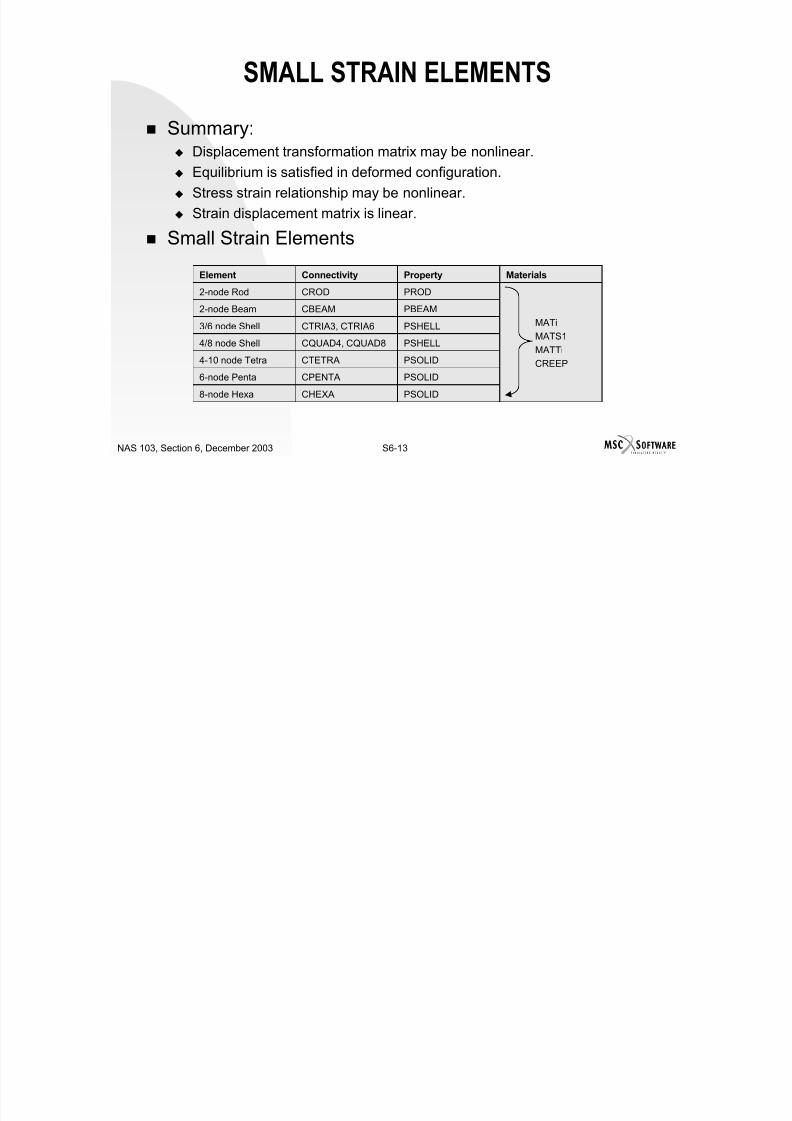
7/21/2019 Nonlinear Analysis Using MSC.nastran
http://slidepdf.com/reader/full/nonlinear-analysis-using-mscnastran 310/783
S6-12NAS 103, Section 6, December 2003
SMALL STRAIN ELEMENTS
Summary: Displacement transformation matrix may be nonlinear. Equilibrium is satisfied in deformed configuration.
Stress strain relationship may be nonlinear.
Strain displacement matrix is linear.
Small Strain Elements
PSOLIDCPENTA6-node Penta
PSOLIDCTETRA4-10 node Tetra
PSHELLCQUAD4, CQUAD84/8 node Shell
MATiMATS1
MATTi
CREEP
PSHELLCTRIA3, CTRIA63/6 node Shell
PBEAMCBEAM2-node Beam
PRODCROD2-node Rod
MaterialsPropertyConnectivityElement
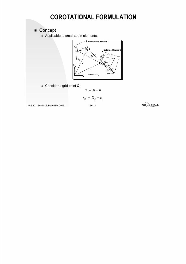
7/21/2019 Nonlinear Analysis Using MSC.nastran
http://slidepdf.com/reader/full/nonlinear-analysis-using-mscnastran 311/783
S6-13NAS 103, Section 6, December 2003
PSOLIDCHEXA8-node Hexa
PSOLIDCPENTA6 node Penta
COROTATIONAL FORMULATION
Concept Applicable to small strain elements.
Consider a grid point Q.x X u+
Undeformed Element
Deformed Elemente1 Xe
e2
X0
b2
b1
Q'
O' d1
xe
u
x
x0
X
d2
wd
u
QO
u0
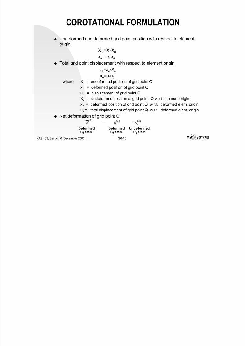
7/21/2019 Nonlinear Analysis Using MSC.nastran
http://slidepdf.com/reader/full/nonlinear-analysis-using-mscnastran 312/783
S6-14NAS 103, Section 6, December 2003
x X u+=
x0
X0
u0
+=
COROTATIONAL FORMULATION
Undeformed and deformed grid point position with respect to elementorigin.
Xe =X-X0
xe = x-x0
Total grid point displacement with respect to element origin
ue=xe-Xe
ue=u-u0
where X = undeformed position of grid point Q
x = deformed position of grid point Q
u = displacement of grid point Q
Xe = undeformed position of grid point Q w.r.t. element originxe = deformed position of grid point Q w.r.t. deformed elem. origin
ue = total displacement of grid point Q w.r.t. deformed elem. origin
Net deformation of grid point Q

7/21/2019 Nonlinear Analysis Using MSC.nastran
http://slidepdf.com/reader/full/nonlinear-analysis-using-mscnastran 313/783
S6-15NAS 103, Section 6, December 2003
g p
Ud( )
xe
d( ) Xe
e( )–=
DeformedSystem
DeformedSystem
UndeformedSystem
ONE-DIMENSIONAL SMALL STRAIN ELEMENTLIBRARY
ROD, CONROD, TUBE
BEAM
GA
GB
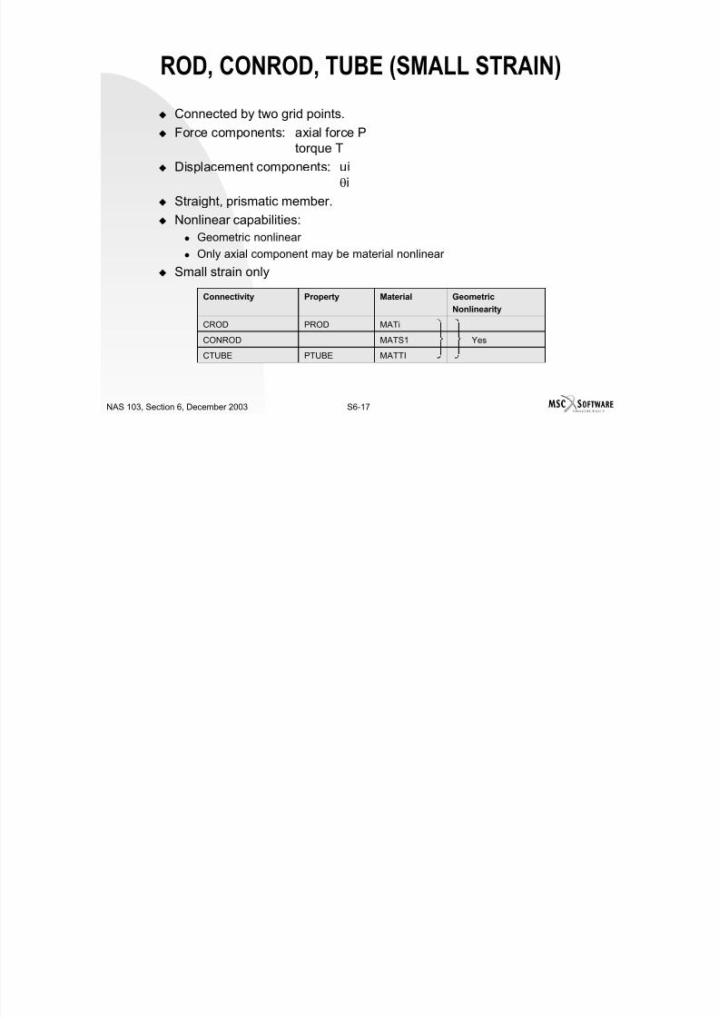
7/21/2019 Nonlinear Analysis Using MSC.nastran
http://slidepdf.com/reader/full/nonlinear-analysis-using-mscnastran 314/783
S6-16NAS 103, Section 6, December 2003
ROD, CONROD, TUBE (SMALL STRAIN)
Connected by two grid points.
Force components: axial force Ptorque T
Displacement components: uiθi
Straight, prismatic member.
Nonlinear capabilities: Geometric nonlinear
Only axial component may be material nonlinear
Small strain only
YesMATS1CONROD
MATiPRODCROD
Geometric
Nonlinearity
MaterialPropertyConnectivity

7/21/2019 Nonlinear Analysis Using MSC.nastran
http://slidepdf.com/reader/full/nonlinear-analysis-using-mscnastran 315/783
S6-17NAS 103, Section 6, December 2003
MATTIPTUBECTUBE
ROD, CONROD, TUBE (SMALL STRAIN)
Nonlinear Output Format
NONLINEAR ELEMENT PROBLEM: NLELI65 FEBRUARY 20, 1986 MSC/NASTRAN 11/27/85 PAGE 33
INELASTIC LOADING
CHECK OUTPUT FORMATS FOR NONLINEAR ELEMENTS SUBCASE 2
LOAD STEP = 2.00000E+00
N O N L I N E A R S T R E S S E S I N R O D E L E M E N T S ( C R O D )
ELEMENT AXIAL STRESS EQUIVALENT TOTAL STRAIN EFF. STRAIN EFF. CREEP LIN.TORSIONAL
ID STRESS PLASTIC/NLELAST STRAIN STRESS
8900 4.500000E+04 4.500000E+04 3.000000E-03 1.500000E-03 0.0 0.0

7/21/2019 Nonlinear Analysis Using MSC.nastran
http://slidepdf.com/reader/full/nonlinear-analysis-using-mscnastran 316/783
S6-18NAS 103, Section 6, December 2003
ROD, CONROD, TUBE (SMALL STRAIN)
Linear Output FormatNONLINEAR ELEMENT PROBLEM : NLELI65 FEBRUARY 20, 1986 MSC/NASTRAN 11/27/85 PAGE 52INELASTIC LOADING
CHECK OUTPUT FORMATS FOR NONLINEAR ELEMENTS NONLINEARSUBCASE 2
LOAD STEP = 2.00000E+00
S T R E S S E S I N R O D E L E M E N T S ( C R O D )
ELEMENT AXIAL SAFETY TORSIONAL SAFETY ELEMENT AXIAL SAFETY TORSIONAL
SAFETYID. STRESS MARGIN STRESS MARGIN ID. STRESS MARGIN STRESS
MARGIN
8900 4.500000E+04 0.0

7/21/2019 Nonlinear Analysis Using MSC.nastran
http://slidepdf.com/reader/full/nonlinear-analysis-using-mscnastran 317/783
S6-19NAS 103, Section 6, December 2003
BEAM (SMALL STRAIN)
Connected by two grid points
Element Coordinate System Orientation of cross-sectional bending properties are defined by the third
grid point or orientation vector v. Additional degrees of freedom must be defined for the warping variables
( ti l)
(0,0,0)
znb
Plane 2
Shear Center
Nonstructural MassCenter of Gravity
Neutral Axis
Grid PointGA
Plane 1
yelem
zna
yna
ymazelem
xelem
(xb ,0,0)
ynb
zmb
ymb
zma
Grid PointGB
I1 = Izz
I2 = Iyy
x x vwa Offset
wb Offset
v
Myy
z
Iyy
-------------
Mzz
y
Izz
-------------
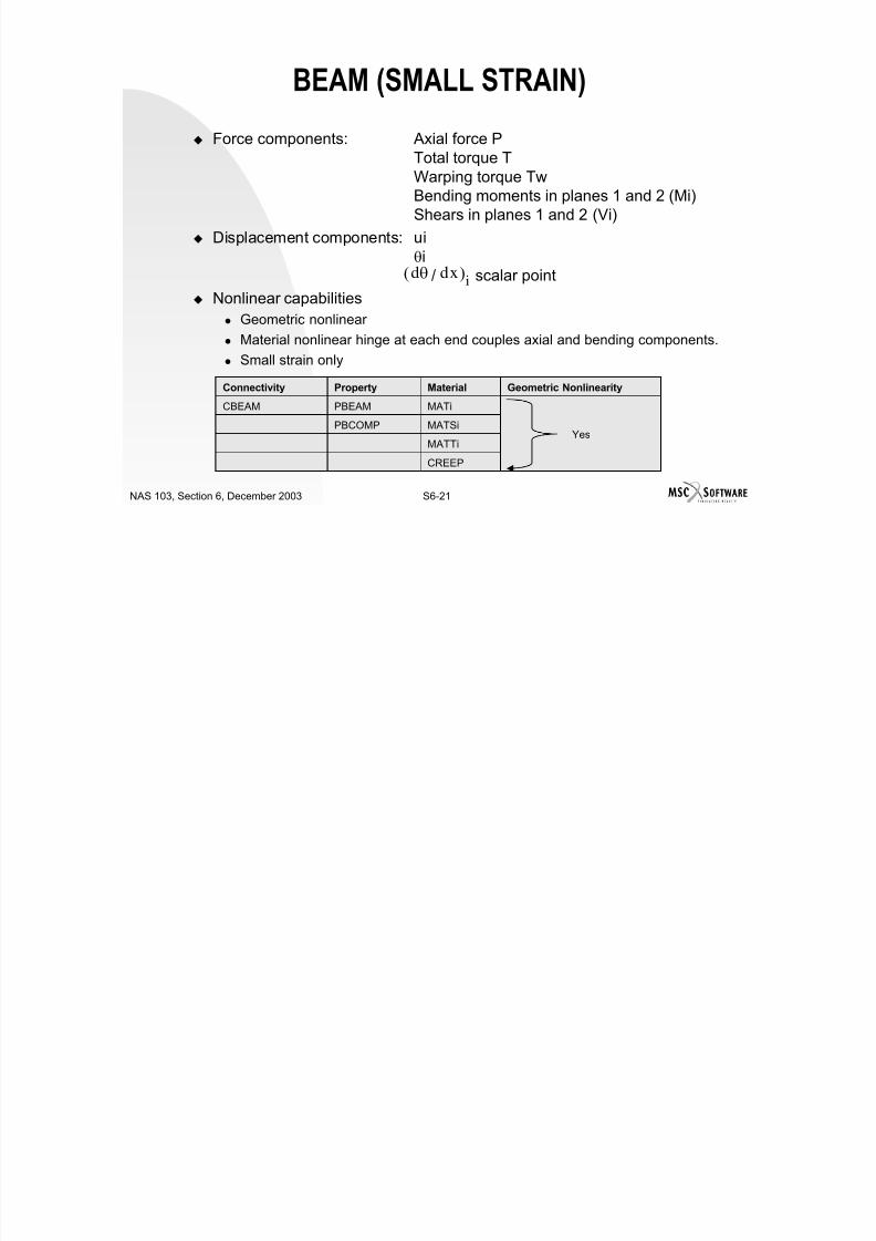
7/21/2019 Nonlinear Analysis Using MSC.nastran
http://slidepdf.com/reader/full/nonlinear-analysis-using-mscnastran 318/783
S6-20NAS 103, Section 6, December 2003
(optional).
BEAM (SMALL STRAIN)
Force components: Axial force PTotal torque TWarping torque TwBending moments in planes 1 and 2 (Mi)Shears in planes 1 and 2 (Vi)
Displacement components: ui
θi / scalar point
Nonlinear capabilities Geometric nonlinear
Material nonlinear hinge at each end couples axial and bending components.
Small strain only
dθ dx( )i
MATSiPBCOMPY
MATiPBEAMCBEAM
Geometric NonlinearityMaterialPropertyConnectivity

7/21/2019 Nonlinear Analysis Using MSC.nastran
http://slidepdf.com/reader/full/nonlinear-analysis-using-mscnastran 319/783
S6-21NAS 103, Section 6, December 2003
CREEP
MATTiYes
BEAM (SMALL STRAIN)
Notes: 1. BAR is not a nonlinear element.2. Any kind of nonlinearity specified for BAR is ignored.
Plastic Hinges for the Beam Element Rationale:
If work-hardening is negligible, a plastic hinge appears in a frame at the pointwhere the bending moment is maximum.
The ratio of the collapse moment to the moment at first yield rangesfrom 1.0 to 2.0 for practical sections.
F i i b l i h d l d l h b di
P
Plastic Zone

7/21/2019 Nonlinear Analysis Using MSC.nastran
http://slidepdf.com/reader/full/nonlinear-analysis-using-mscnastran 320/783
S6-22NAS 103, Section 6, December 2003
For a prismatic beam element with end loads only, the bending moment
is maximum at one end.
BEAM (SMALL STRAIN)
MAT1 ’ MATS1 “Plastic”
Will only yield at grid point.
Plasticity is simulated by eight plastic rods that support extension andbending about two axes (y and z).
Taper is allowed.
l /8
Potential PlasticZones
A B
l
l /8
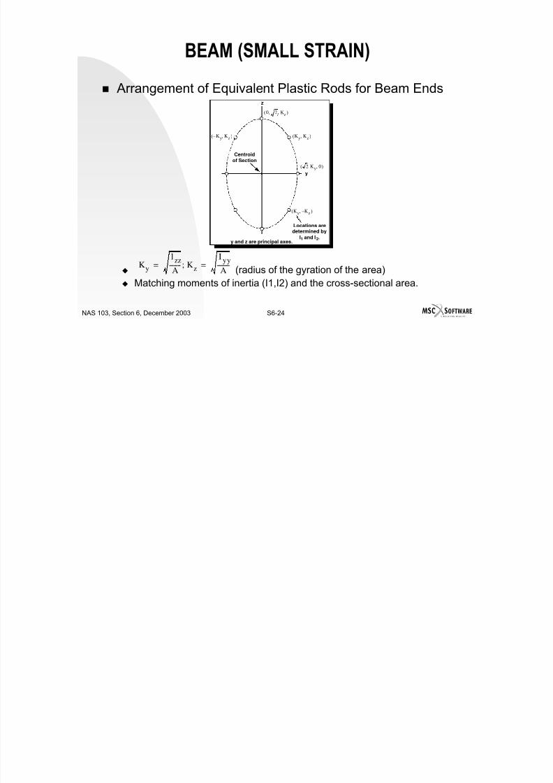
7/21/2019 Nonlinear Analysis Using MSC.nastran
http://slidepdf.com/reader/full/nonlinear-analysis-using-mscnastran 321/783
S6-23NAS 103, Section 6, December 2003
BEAM (SMALL STRAIN)
Arrangement of Equivalent Plastic Rods for Beam Ends
(radius of the gyration of the area)Ky
l zz
A-------- Kz;
I yy
A---------= =
Centroidof Section
y
y and z are principal axes.
Locations aredetermined by
I1 and I2.
z
0 2l Kz,( )
2 Ky 0,( )
Ky Kz–,( )
Ky– Kz,( ) Ky Kz,( )
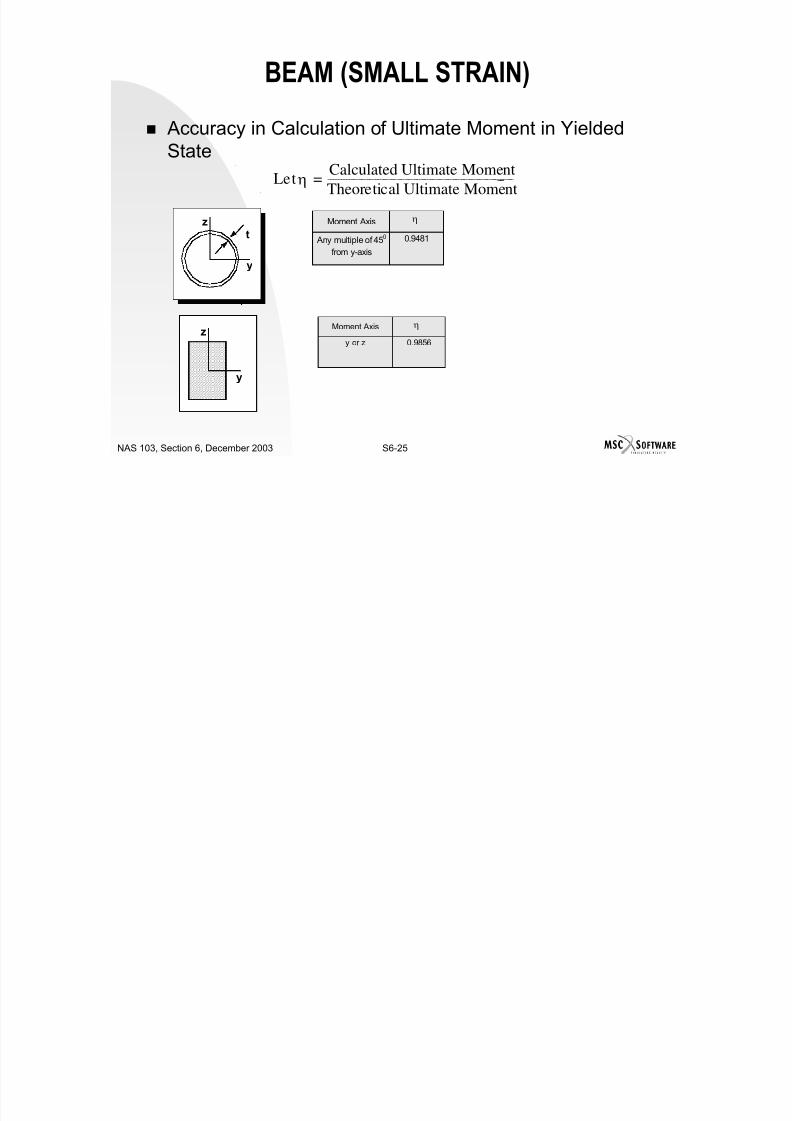
7/21/2019 Nonlinear Analysis Using MSC.nastran
http://slidepdf.com/reader/full/nonlinear-analysis-using-mscnastran 322/783
S6-24NAS 103, Section 6, December 2003
( gy )
Matching moments of inertia (I1,I2) and the cross-sectional area.
BEAM (SMALL STRAIN)
Accuracy in Calculation of Ultimate Moment in Yielded
StateLetη
Calculated Ultimate Moment
Theoretical Ultimate Moment-----------------------------------------------------------------------=
Moment Axis
Any multiple of 450
from y-axis0.9481
η
Moment Axis
y or z 0.9856
η
t
z
y
z
y
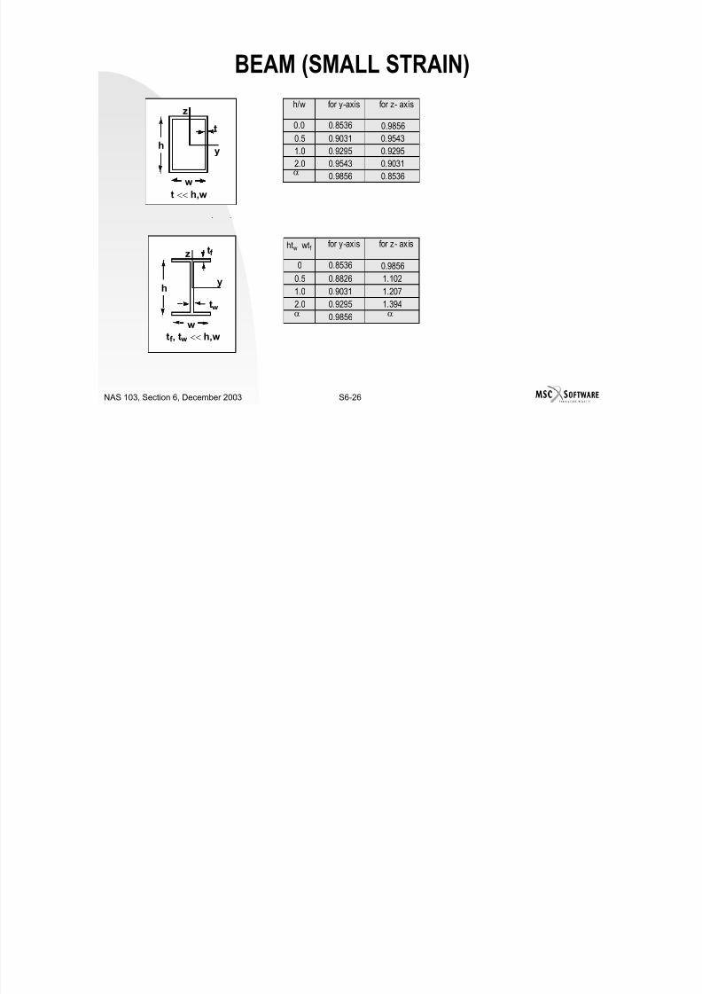
7/21/2019 Nonlinear Analysis Using MSC.nastran
http://slidepdf.com/reader/full/nonlinear-analysis-using-mscnastran 323/783
S6-25NAS 103, Section 6, December 2003
BEAM (SMALL STRAIN)
htw wtf for y-axis for z- axis
0 0.8536 0.9856
0.5 0.8826 1.102
1.0 0.9031 1.207
2.0 0.9295 1.394
0.9856α α
h/w for y-axis for z- axis
0.0 0.8536 0.9856
0.5 0.9031 0.95431.0 0.9295 0.9295
2.0 0.9543 0.9031
0.9856 0.8536α
z
y
t
w
t << h,w
h
tf z
y
w
tw
tf , tw << h,w
h

7/21/2019 Nonlinear Analysis Using MSC.nastran
http://slidepdf.com/reader/full/nonlinear-analysis-using-mscnastran 324/783
S6-26NAS 103, Section 6, December 2003
BEAM (SMALL STRAIN)
Limitations of Nonlinear Beam Elements
The material is assumed to be elastic-perfectly plastic. Work hardeningcan cause errors since results depend on beam length.
Any material nonlinearity other than elastic-perfectly plastic will yieldincorrect answers.
Treatment for torsion, warping, and transverse shear is linear.
Pin-flags are not allowed for material nonlinear analysis, i.e., theycannot be used with MATS1, MATT1, or CREEP Bulk Data entries.However, pin-flags can be used for geometric nonlinear analysis.
Offsets are not allowed for geometric nonlinear analysis.
Linear or nonlinear buckling analysis with offsets may give wrongresults.
No distributed loads (PLOAD1) are allowed.

7/21/2019 Nonlinear Analysis Using MSC.nastran
http://slidepdf.com/reader/full/nonlinear-analysis-using-mscnastran 325/783
S6-27NAS 103, Section 6, December 2003
BEAM (SMALL STRAIN)
Nonlinear Output FormatN O N L I N E A R O U T P U T F O R B E A M
NONLINEAR ELEMENT PROBLEM: NLELI65 FEBRUARY 20, 1986 MSC/NASTRAN 11/27/85PAGE 30
INELASTIC LOADING
CHECK OUTPUT FORMATS FOR NONLINEAR ELEMENTSSUBCASE 2
LOAD STEP = 2.00000E+00
N O N L I N E A R S T R E S S E S I N B E A M E L E M E N T S ( C B E A M )
ELEMENT GRID POINT STRESS EQUIVALENT TOTAL STRAIN EFF. STRAIN EFF.
CREEPID ID STRESS PLASTIC/NLELAST
STRAIN9400 9401 C -4.973799E-14 0.0 -1.657933E-21 0.0 0.0
D 3.000000E+04 3.000000E+04 1.046283E-03 4.628333E-05 0.0E -4.973799E-14 0.0 -1.657933E-21 0.0 0.0F -3.000000E+04 3.000000E+04 -1.046283E-03 4.628333E-05 0.0
9402 C 7.105427E-15 0.0 2.368476E-22 0.0 0.0
D -1.153490E-12 0.0 -3.844965E-20 0.0 0.0E 7.105427E-15 0.0 2.368476E-22 0.0 0.0
F 1.167700E-12 0.0 3.892335E-20 0.0 0.0

7/21/2019 Nonlinear Analysis Using MSC.nastran
http://slidepdf.com/reader/full/nonlinear-analysis-using-mscnastran 326/783
S6-28NAS 103, Section 6, December 2003
BEAM (SMALL STRAIN)
Linear Output Format
NONLINEAR ELEMENT PROBLEM: NLELI65 FEBRUARY 20, 1986 MSC/NASTRAN
11/27/85 PAGE 48INELASTIC LOADING
CHECK OUTPUT FORMATS FOR NONLINEAR ELEMENTS NONLINEARSUBCASE 2
LOAD STEP = 2.00000E+00
S T R E S S E S I N B E A M E L E M E N T S ( C B E A M )
STAT DIST/ELEMENT-ID GRID LENGTH SXC SXD SXE SXF S-MAX S-MINM.S.-T M.S.-C
9400 9401 0.000 -4.973799E-14 3.000000E+04 -4.973799E-14 -3.000000E+04 3.000000E+04 -3.000000E+049402 1.000 7.105427E-15 -1.153490E-12 7.105427E-15 1.167700E-12 1.167700E-12 -1.153490E-12
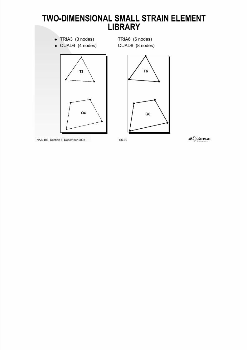
7/21/2019 Nonlinear Analysis Using MSC.nastran
http://slidepdf.com/reader/full/nonlinear-analysis-using-mscnastran 327/783
S6-29NAS 103, Section 6, December 2003
TWO-DIMENSIONAL SMALL STRAIN ELEMENTLIBRARY
TRIA3 (3 nodes) TRIA6 (6 nodes)
QUAD4 (4 nodes) QUAD8 (8 nodes)
T3
Q4
T6
Q8

7/21/2019 Nonlinear Analysis Using MSC.nastran
http://slidepdf.com/reader/full/nonlinear-analysis-using-mscnastran 328/783
S6-30NAS 103, Section 6, December 2003
NONLINEAR SHELL AND PLATE ELEMENTS
QUAD4 and TRIA3
Isoparametric elements: QUAD4 and TRIA3. Membrane and plate bending applicable to nonlinear material.
Transverse shear (Mindlin) remains linear.
Simulate thick or thin curved shell.
QUAD4 is preferred. TRIA3 is too stiff in membrane. Each connecting node has 6 DOFs. Stiffness is not defined for rotation
about the normal to the plane. Therefore, use K6ROT.
Midplane offset may be used for geometric nonlinear only.
Pass constant stress patch test.
No shear locking, no spurious modes.
Poisson’s ratio locking exists, especially in plane strain.
Use of offsets will cause incorrect results in buckling analysis anddifferential stiffness.

7/21/2019 Nonlinear Analysis Using MSC.nastran
http://slidepdf.com/reader/full/nonlinear-analysis-using-mscnastran 329/783
S6-31NAS 103, Section 6, December 2003
NONLINEAR SHELL AND PLATE ELEMENTS
QUAD4: Connected by four grid points. The orientation of the normal to
the surface is defined by the connectivity. TRIA3: Connected by three grid points. The orientation of the normal
to the surface is defined by the connectivity.
Force components: Membrane forces Fx, Fy, Fxy
Bending moments Mx, My, MxyTransverse shear forces Qx, Qy
Stress components: σx, σy, τxy (at center)
Displacement components: ui
θx, θy (no rotation normal to element)

7/21/2019 Nonlinear Analysis Using MSC.nastran
http://slidepdf.com/reader/full/nonlinear-analysis-using-mscnastran 330/783
S6-32NAS 103, Section 6, December 2003
NONLINEAR SHELL AND PLATE ELEMENTS
QUAD8 and TRIA6
Isoparametric elements: QUAD8 and TRIA6. Membrane and plate bending applicable to nonlinear material.
Transverse shear (Mindlin) remains linear.
Simulate thick or thin curved shell.
Each connecting node has 6 DOFs. Stiffness is not defined for rotationabout the normal to the plane. Therefore, use K6ROT.
Midplane offset may be used for geometric nonlinear only.
Pass constant stress patch test.
Use of offsets will cause incorrect results in buckling analysis and
differential stiffness.

7/21/2019 Nonlinear Analysis Using MSC.nastran
http://slidepdf.com/reader/full/nonlinear-analysis-using-mscnastran 331/783
S6-33NAS 103, Section 6, December 2003
NONLINEAR SHELL AND PLATE ELEMENTS
QUAD8: Connected by eight grid points. The orientation of the normal to
the surface is defined by the connectivity. TRIA6: Connected by three grid points. The orientation of the normal
to the surface is defined by the connectivity.
Force components: Membrane forces Fx, Fy, Fxy
Bending moments Mx, My, MxyTransverse shear forces Qx, Qy
Stress components: σx, σy, τxy (at center)
Displacement components: ui
θx, θy (no rotation normal to element)

7/21/2019 Nonlinear Analysis Using MSC.nastran
http://slidepdf.com/reader/full/nonlinear-analysis-using-mscnastran 332/783
S6-34NAS 103, Section 6, December 2003
NONLINEAR SHELL AND PLATE ELEMENTS
Nonlinear capabilities: Geometric nonlinear
Material nonlinear for membrane and bending components
CREEPCTRIA6
MATTiCQUAD8
MATS1CTRIA3
YesMATiPSHELLCQUAD4
Geometric
Nonlinearity
MaterialPropertyConnectivity

7/21/2019 Nonlinear Analysis Using MSC.nastran
http://slidepdf.com/reader/full/nonlinear-analysis-using-mscnastran 333/783
S6-35NAS 103, Section 6, December 2003
OUTPUT FOR SHELL AND PLATE ELEMENTS
Nonlinear Format
NONLINEAR ELEMENT PROBLEM: NLELI65 FEBRUARY 20, 1986 MSC/NASTRAN 11/27/85PAGE 34INELASTIC LOADING
CHECK OUTPUT FORMATS FOR NONLINEAR ELEMENTSSUBCASE 2LOAD STEP = 2.00000E+00
N O N L I N E A R S T R E S S E S I N T R I A N G U L A R E L E M E N T S ( T R I A 3 )
ELEMENT FIBRE STRESSES/ TOTAL STRAINS EQUIVALENT EFF. STRAIN EFF.CREEPID DISTANCE X Y Z XY STRESS PLASTIC/NLELAST
STRAIN
8800 -5.000000E-02 4.504111E+04 1.015688E+02 -6.266323E-14 4.499041E+04 1.499041E-03 0.02.993653E-03 -8.078549E-04 0.0
5.000000E-02 4.504111E+04 1.015688E+02 -6.266323E-14 4.499041E+04 1.499041E-03 0.02.993653E-03 -8.078549E-04 0.0
8801 -5.000000E-02 2.257134E+04 2.257134E+04 -2.246977E+04 4.499041E+04 1.499041E-03 0.01.092899E-03 1.092899E-03 -3.801508E-03
5.000000E-02 2.257134E+04 2.257134E+04 -2.246977E+04 4.499041E+04 1.499041E-03 0.0
1.092899E-03 1.092899E-03 -3.801508E-03

7/21/2019 Nonlinear Analysis Using MSC.nastran
http://slidepdf.com/reader/full/nonlinear-analysis-using-mscnastran 334/783
S6-36NAS 103, Section 6, December 2003
OUTPUT FOR SHELL AND PLATE ELEMENTS
Linear Format
NONLINEAR ELEMENT PROBLEM: NLELI65 FEBRUARY 20, 1986 MSC/NASTRAN11/27/85 PAGE 53
INELASTIC LOADING
CHECK OUTPUT FORMATS FOR NONLINEAR ELEMENTS NONLINEARSUBCASE 2LOAD STEP = 2.00000E+00
S T R E S S E S I N T R I A N G U L A R E L E M E N T S ( T R I A 3 )
ELEMENT FIBRE STRESSES IN ELEMENT COORD SYSTEM PRINCIPAL STRESSES (ZERO SHEAR)
ID. DISTANCE NORMAL-X NORMAL-Y SHEAR-XY ANGLE MAJOR MINORVON MISES8800 -5.000000E-02 4.504111E+04 1.015688E+02 -6.266323E-14 0.0000 4.504111E+04 1.015688E+02
4.499041E+045.000000E-02 4.504111E+04 1.015688E+02 -6.266323E-14 0.0000 4.504111E+04 1.015688E+02
4.499041E+048801 -5.000000E-02 2.257134E+04 2.257134E+04 -2.246977E+04 -45.0000 4.504111E+04 1.015688E+02
4.499041E+045.000000E-02 2.257134E+04 2.257134E+04 -2.246977E+04 -45.0000 4.504111E+04 1.015688E+02
4.499041E+04
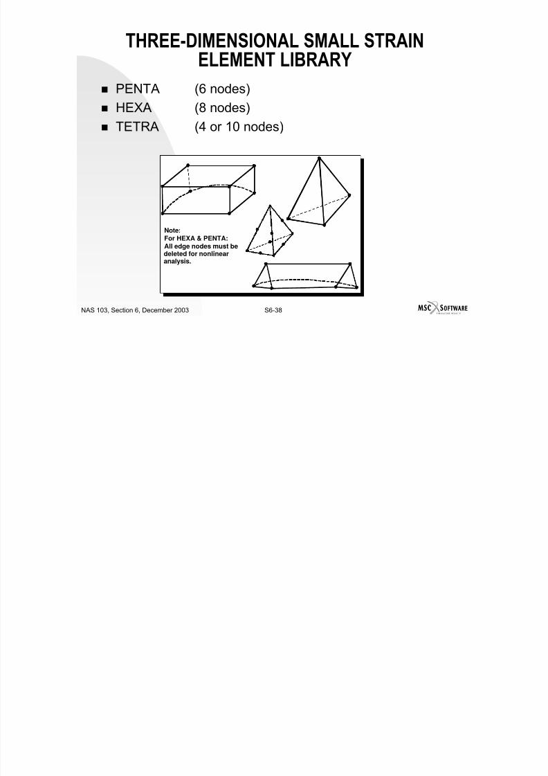
7/21/2019 Nonlinear Analysis Using MSC.nastran
http://slidepdf.com/reader/full/nonlinear-analysis-using-mscnastran 335/783
S6-37NAS 103, Section 6, December 2003
THREE-DIMENSIONAL SMALL STRAINELEMENT LIBRARY
PENTA (6 nodes)
HEXA (8 nodes) TETRA (4 or 10 nodes)
Note:For HEXA & PENTA:All edge nodes must bedeleted for nonlinearanalysis.
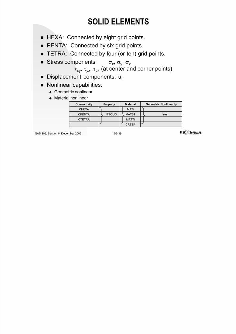
7/21/2019 Nonlinear Analysis Using MSC.nastran
http://slidepdf.com/reader/full/nonlinear-analysis-using-mscnastran 336/783
S6-38NAS 103, Section 6, December 2003
SOLID ELEMENTS
HEXA: Connected by eight grid points.
PENTA: Connected by six grid points. TETRA: Connected by four (or ten) grid points.
Stress components: σx, σy, σz
τxy
, τyz
, τzx
(at center and corner points)
Displacement components: ui
Nonlinear capabilities: Geometric nonlinear
Material nonlinear
MATTiCTETRA
YesMATS1PSOLIDCPENTA
MATiCHEXA
Geometric NonlinearityMaterialPropertyConnectivity

7/21/2019 Nonlinear Analysis Using MSC.nastran
http://slidepdf.com/reader/full/nonlinear-analysis-using-mscnastran 337/783
S6-39NAS 103, Section 6, December 2003
CREEP
SOLID ELEMENTS
Note: 1. HEXA20 and PENTA15 are not nonlinear elements.
2. Any kind of nonlinearity specified for HEXA20 andPENTA15 is ignored.
Uses the strain function formulation that improves accuracy as
Poisson’s ratio approaches one-half. Internal degrees of freedom areintroduced to approximate quadratic shape function (for HEXA andPENTA only).

7/21/2019 Nonlinear Analysis Using MSC.nastran
http://slidepdf.com/reader/full/nonlinear-analysis-using-mscnastran 338/783
S6-40NAS 103, Section 6, December 2003

7/21/2019 Nonlinear Analysis Using MSC.nastran
http://slidepdf.com/reader/full/nonlinear-analysis-using-mscnastran 339/783
SOLID ELEMENTS
Nonlinear Output Format
1 ELASTIC-PLASTIC BUCKLING OF IMPERFECT SPHERICAL SHELL N10657 DECEMBER 2, 1993 MSC/NASTRAN 12/ 1/93 PAGE 177HYDROSTATIC PRESSURE APPLIED,PERIPHERY CLAMPED
0 SUBCASE 3LOAD STEP = 3.00000E+00
N O N L I N E A R S T R E S S E S I N H E X A H E D R O N S O L I D E L E M E N T S ( H E X A )
ELEMENT GRID/ POINT STRESSES/ TOTAL STRAINS EQUIVALENT EFF. STRAIN EFF. CREEPID GAUSS ID X Y Z XY YZ ZX STRESS PLAS/NLELAS STRAIN
0 11 GRID CENTER 5.8398E+04 4.4519E+04 -2.0017E+04 -3.0549E-08 3.1213E-08 3.7113E+02 7.8000E+04 2.3300E-02 .02.6695E-03 5.3108E-04 -1.3093E-04 -6.1377E-15 7.6010E-15 1.4537E-03
101 -1.6090E+05 -4.6212E+04 4.0530E+04 -1.8137E-07 7.5895E-08 -9.9750E+02 6.4259E+04 9.9663E-02 .0-9.1663E-02 -1.6827E-02 1.0228E-01 1.5330E-14 5.2356E-15 1.4537E-03
103 -1.3510E+05 -1.5007E+05 -3.2840E+04 -2.0672E-07 -1.3284E-08 -1.0080E+02 2.4847E+04 7.8079E-02 .0-5.1229E-02 -4.3337E-02 8.2691E-02 1.5330E-14 9.9665E-15 1.4537E-03
104 -1.3510E+05 -1.5007E+05 -3.2840E+04 -2.0672E-07 -1.3284E-08 -1.0080E+02 2.4847E+04 7.8079E-02 .0-5.1229E-02 -4.3337E-02 8.2691E-02 1.5330E-14 9.9665E-15 1.4537E-03
102 -1.6090E+05 -4.6212E+04 4.0530E+04 -1.8137E-07 7.5895E-08 -9.9750E+02 6.4259E+04 9.9663E-02 .0-9.1663E-02 -1.6827E-02 1.0228E-01 1.5330E-14 5.2356E-15 1.4537E-03
201 2.4837E+05 1.5368E+05 1.6060E+04 -2.5726E-08 8.0401E-08 -3.5225E+02 7.8000E+04 1.0156E-01 .01.0069E-01 1.7070E-02 -1.0227E-01 -2.7606E-14 5.2356E-15 1.4537E-03
203 1.9665E+05 1.8168E+05 2.0698E+04 -2.8129E-08 -1.7611E-08 -2.8327E+02 7.8000E+04 7.5058E-02 .05.2881E-02 4.5218E-02 -8.3228E-02 -2.7606E-14 9.9665E-15 1.4537E-03
204 1.9665E+05 1.8168E+05 2.0698E+04 -2.8129E-08 -1.7611E-08 -2.8327E+02 7.8000E+04 7.5058E-02 .05.2881E-02 4.5218E-02 -8.3228E-02 -2.7606E-14 9.9665E-15 1.4537E-03
202 2.4837E+05 1.5368E+05 1.6060E+04 -2.5726E-08 8.0401E-08 -3.5225E+02 7.8000E+04 1.0156E-01 .01.0069E-01 1.7070E-02 -1.0227E-01 -2.7606E-14 5.2356E-15 1.4537E-03

7/21/2019 Nonlinear Analysis Using MSC.nastran
http://slidepdf.com/reader/full/nonlinear-analysis-using-mscnastran 340/783
S6-42NAS 103, Section 6, December 2003
LARGE STRAIN ELEMENTS
General:
Can have large displacements and rotation. Only isotropic hyperelastic material is available (MATHP).
Strain to displacement matrix is nonlinear.
Equilibrium is satisfied in deformed configuration.

7/21/2019 Nonlinear Analysis Using MSC.nastran
http://slidepdf.com/reader/full/nonlinear-analysis-using-mscnastran 341/783
S6-43NAS 103, Section 6, December 2003
HYPERELASTIC ELEMENTS
Hyperelastic element characteristics:
All hyperelastic elements have hyperelastic materials only (MATHP BulkData entry). Hyperelastic material includes linear elastic material.
Total Lagrangian formulation with updated coordinates.
Green strain potential function.
Energy conjugate stress-strain pair: Cauchy stress and symmetric part
of the virtual displacement gradient. Deformation is split into volumetric and distortional components.
Mixed formulation: Separate interpolation for displacements andvolume ratio/pressure.

7/21/2019 Nonlinear Analysis Using MSC.nastran
http://slidepdf.com/reader/full/nonlinear-analysis-using-mscnastran 342/783
S6-44NAS 103, Section 6, December 2003
HYPERELASTIC ELEMENTS
Avoids volumetric locking for nearly incompressible material.
Stiffness matrix is divided into material and geometric parts. Geometric part is included by PARAM,LGDISP,1.
It is strongly recommended that PARAM,LGDISP,1 be used.
Temperature loads can be specified for all elements.
Follower pressure loads are available for all elements.
Missing grids (e.g., 5 node CQUAD) are not recommended.
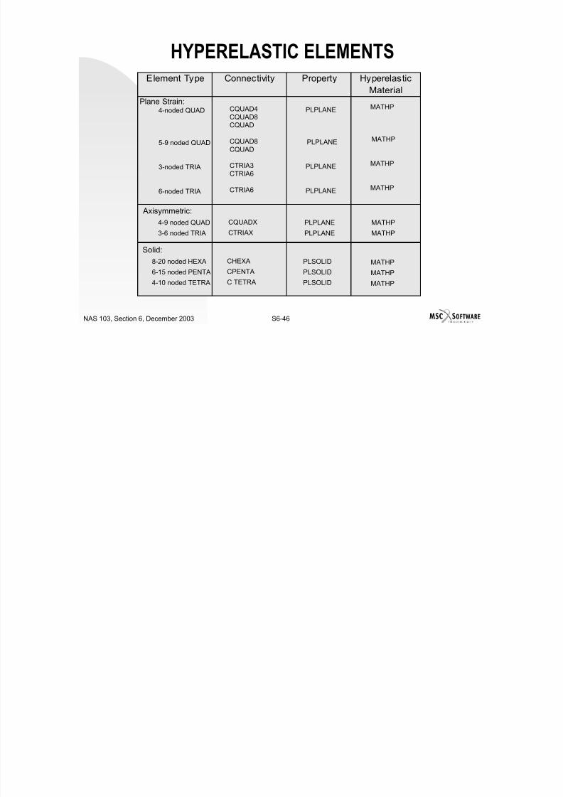
7/21/2019 Nonlinear Analysis Using MSC.nastran
http://slidepdf.com/reader/full/nonlinear-analysis-using-mscnastran 343/783
S6-45NAS 103, Section 6, December 2003
HYPERELASTIC ELEMENTSElement Type Connectivity Property Hyperelastic
MaterialPlane Strain:
4-noded QUAD
5-9 noded QUAD
3-noded TRIA
6-noded TRIA
CQUAD4CQUAD8CQUAD
CQUAD8CQUAD
CTRIA3
CTRIA6
CTRIA6
PLPLANE
PLPLANE
PLPLANE
PLPLANE
MATHP
MATHP
MATHP
MATHP
Axisymmetric:
4-9 noded QUAD
3-6 noded TRIA
CQUADX
CTRIAX
PLPLANE
PLPLANE
MATHP
MATHP
Solid:
8-20 noded HEXA
6-15 noded PENTA
4-10 noded TETRA
CHEXA
CPENTA
C TETRA
PLSOLID
PLSOLID
PLSOLID
MATHP
MATHP
MATHP
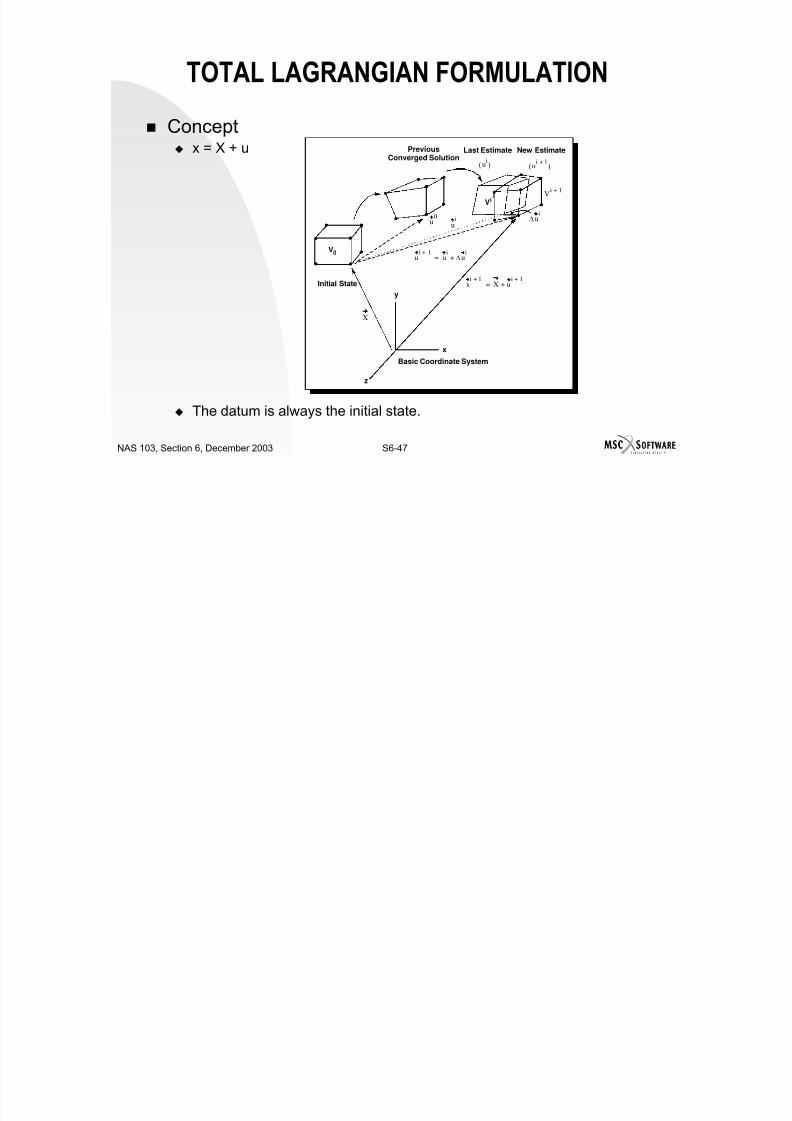
7/21/2019 Nonlinear Analysis Using MSC.nastran
http://slidepdf.com/reader/full/nonlinear-analysis-using-mscnastran 344/783
S6-46NAS 103, Section 6, December 2003
TOTAL LAGRANGIAN FORMULATION
Concept x = X + u
The datum is always the initial state
Previous
Converged Solution
Initial State
Last Estimate
x
z
Basic Coordinate System
New Estimate
Vi
V0
ui( ) u
i 1+( )
Vi 1+
∆ui
uiu
0
X
ui 1+
ui
∆ui
+=
xi 1+
X ui 1+
+=
y

7/21/2019 Nonlinear Analysis Using MSC.nastran
http://slidepdf.com/reader/full/nonlinear-analysis-using-mscnastran 345/783
S6-47NAS 103, Section 6, December 2003
The datum is always the initial state.
TOTAL LAGRANGIAN FORMULATION Hyperelastic elements use the updated coordinates to form the
stiffness matrix.
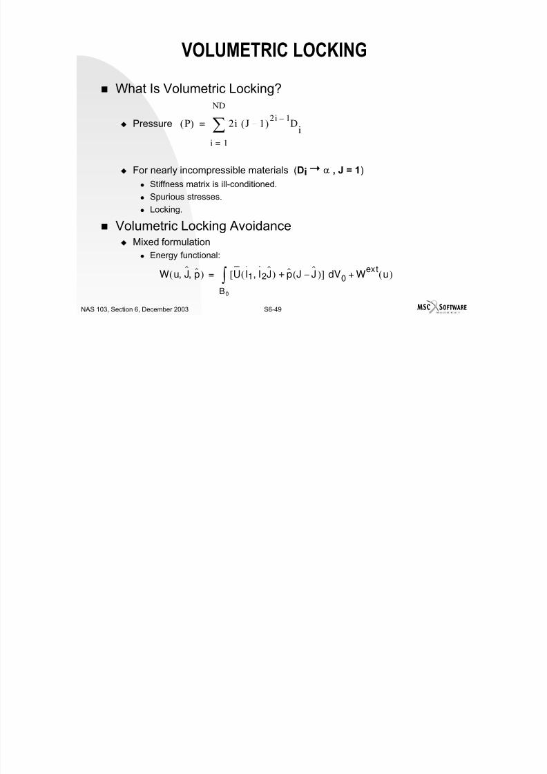
7/21/2019 Nonlinear Analysis Using MSC.nastran
http://slidepdf.com/reader/full/nonlinear-analysis-using-mscnastran 346/783
S6-48NAS 103, Section 6, December 2003
VOLUMETRIC LOCKING
What Is Volumetric Locking?
Pressure
For nearly incompressible materials (Di α , J = 1) Stiffness matrix is ill-conditioned.
Spurious stresses.
Locking.
Volumetric Locking Avoidance Mixed formulation
Energy functional:
P( ) 2i J 1–( )2i 1–
Di
i 1=
ND
∑=
W u J p, ,( ) U I1 I2J,( ) p J J–( )+[ ] V0 Wext
u( )+d
B0
∫=
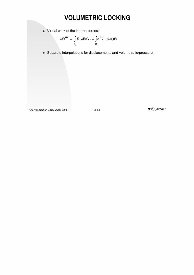
7/21/2019 Nonlinear Analysis Using MSC.nastran
http://slidepdf.com/reader/full/nonlinear-analysis-using-mscnastran 347/783
S6-49NAS 103, Section 6, December 2003
B0
VOLUMETRIC LOCKING
Virtual work of the internal forces:
Separate interpolations for displacements and volume ratio/pressure.
δWint
ST
δE V0 σT
∇S
δu( ) VdB∫
=dB0∫=

7/21/2019 Nonlinear Analysis Using MSC.nastran
http://slidepdf.com/reader/full/nonlinear-analysis-using-mscnastran 348/783
S6-50NAS 103, Section 6, December 2003
OUTPUT FOR HYPERELASTIC ELEMENTS
Cauchy stress σ
Defined from
where df = force in the deformed state
n = unit normal to the deformed areadA = deformed area
df σn dA=
x-y plane of basic Axisymmetricx-y plane of user-specified coordinate system; default=basicPlain Strain
BasicSolids
Output Coordinate SystemElements

7/21/2019 Nonlinear Analysis Using MSC.nastran
http://slidepdf.com/reader/full/nonlinear-analysis-using-mscnastran 349/783
S6-51NAS 103, Section 6, December 2003
OUTPUT FOR HYPERELASTIC ELEMENTS
Logarithmic strain
where λi = principal stretchesNi = unit vectors in the principal directions
ε ln λi N i N iT
i 1=
3
∑=

7/21/2019 Nonlinear Analysis Using MSC.nastran
http://slidepdf.com/reader/full/nonlinear-analysis-using-mscnastran 350/783
S6-52NAS 103, Section 6, December 2003
OUTPUT FOR HYPERELASTIC ELEMENTS
Note that in case of temperature strains, the total strains are output
Pressure (tension is positive)
Volumetric strain (volume increase is positive)
where J = det F Linear and nonlinear output format is available.
Output may be requested in SORT1 or SORT2.
SORT2 is applicable to linear format.
ε σ
E--- α∆T+=
p1
3--- tr σ=
εV
J 1= -

7/21/2019 Nonlinear Analysis Using MSC.nastran
http://slidepdf.com/reader/full/nonlinear-analysis-using-mscnastran 351/783
S6-53NAS 103, Section 6, December 2003
HYPERELASTIC ELEMENT LIMITATIONS
Fully incompressible material is not available yet; nearly
incompressible material is Poisson’s ratiov ≤ 0.4995 or D1 ≤ 1000. (A10 + A01)
Hyperelastic elements are only available in SOLs 106and 129 and are not available in SOL 66 or SOL 99.
SOL 101 does not produce a fatal error; however, itgives the wrong results.
Stress and strain output only in basic with no grid point
stress output, no center stress output and no user-defined coordinate system for output.

7/21/2019 Nonlinear Analysis Using MSC.nastran
http://slidepdf.com/reader/full/nonlinear-analysis-using-mscnastran 352/783
S6-54NAS 103, Section 6, December 2003
PLANAR HYPERELASTIC ELEMENTS
Plane strain: QUAD4, QUAD8, QUAD, TRIA3, TRIA6,
TRIA. Axisymmetric: QUADX, TRIAX.
Properties are specified by PLPLANE.
PLPLANE Bulk Data Entry Defines a finite deformation plane strain element.
Format:
Example:
CIDMIDPIDPLPLANE
10987654321
201204203PLPLANE

7/21/2019 Nonlinear Analysis Using MSC.nastran
http://slidepdf.com/reader/full/nonlinear-analysis-using-mscnastran 353/783
S6-55NAS 103, Section 6, December 2003
PLANAR HYPERELASTIC ELEMENTSField Contents
PID Element property identification number. (Integer > 0).
MID Identification number of MATHP entry. (Integer > 0).Identification number of a coordinate system defining theplane of deformation.
CID See Remarks 2 and 3. (Integer Š 0; Default = 0).
Remarks:1. PLPLANE can be referenced by a CQUAD, CQUAD4, CQUAD8, CQUADX,
CTRIA3, CTRIA6, or CTRIAX entry.
2. Plane strain hyperelastic elements must lie on the x-y plane of the CID coordinate
system. Stresses and strains are output in the CID coordinate system.3. Axisymmetric hyperelastic elements must lie on the x-y plane of the basic
coordinate system. CID may not be specified and stresses and strains are output inthe basic coordinate system.

7/21/2019 Nonlinear Analysis Using MSC.nastran
http://slidepdf.com/reader/full/nonlinear-analysis-using-mscnastran 354/783
S6-56NAS 103, Section 6, December 2003
PLANAR HYPERELASTIC ELEMENTS ID must be unique between PSHELL and PLPLANE; otherwise, User Fatal
Message 5410 is issued.
Fatal Error 6438 is issued if MATHP is not specified.
Output is in terms of Cauchy stress/log strains in the x-y plane of thereferred coordinate system at each Gauss point.
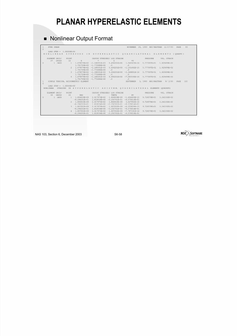
7/21/2019 Nonlinear Analysis Using MSC.nastran
http://slidepdf.com/reader/full/nonlinear-analysis-using-mscnastran 355/783
S6-57NAS 103, Section 6, December 2003
PLANAR HYPERELASTIC ELEMENTS
Nonlinear Output Format1 PURE SHEAR NOVEMBER 18, 1993 MSC/NASTRAN 11/17/93 PAGE 830
LOAD STEP = 1.00000E+00N O N L I N E A R S T R E S S E S I N H Y P E R E L A S T I C Q U A D R I L A T E R A L E L E M E N T S ( QUADFD )
ELEMENT GRID/ POINT CAUCHY STRESSES/ LOG STRAINS PRESSURE VOL. STRAINID GAUSS ID X Y Z XY
0 1 GAUS 1 1.678579E+02 -1.188351E-03 5.456201E+00 1.560323E-16 5.777097E+01 1.925699E-021.791759E+00 -1.772686E+00 .0 .0
2 1.678579E+02 -1.188351E-03 5.456201E+00 -1.191492E-15 5.777097E+01 1.925699E-021.791759E+00 -1.772686E+00 .0 .0
3 1.678579E+02 -1.188351E-03 5.456201E+00 -3.368891E-16 5.777097E+01 1.925699E-02
1.791759E+00 -1.772686E+00 .0 .04 1.678579E+02 -1.188351E-03 5.456201E+00 -7.083336E-16 5.777097E+01 1.925699E-02
1.791759E+00 -1.772686E+00 .0 .01 SIMPLE TENSION, AXISYMMETRIC ELEMENT SEPTEMBER 3, 1993 MSC/NASTRAN 9/ 2/93 PAGE 1030
LOAD STEP = 1.00000E+00NONLINEAR STRESSES IN H Y P E R E L A S T I C A X I S Y M M. Q U A D R I L A T E R A L ELEMENTS (QUADXFD)
ELEMENT GRID/ POINT CAUCHY STRESSES/ LOG STRAINS PRESSURE VOL. STRAINID GAUSS ID RAD YY THETA RY
0 1 GAUS 1 1.806839E-09 2.917973E+02 1.806839E-09 -1.456493E-15 9.726578E+01 3.242192E-02
-8.296252E-01 1.818534E+00 -3.250761E-01 -9.570014E-012 1.806910E-09 2.917973E+02 1.806910E-09 3.027552E-16 9.726578E+01 3.242192E-02
-8.296252E-01 1.818534E+00 -3.250761E-01 -9.570014E-013 1.807052E-09 2.917973E+02 1.807052E-09 -6.255834E-15 9.726578E+01 3.242192E-02
-8.296252E-01 1.818534E+00 -3.250761E-01 -9.570014E-01
4 1.807052E-09 2.917973E+02 1.807052E-09 -7.787191E-16 9.726578E+01 3.242192E-02-8.296252E-01 1.818534E+00 -3.250761E-01 -9.570014E-01
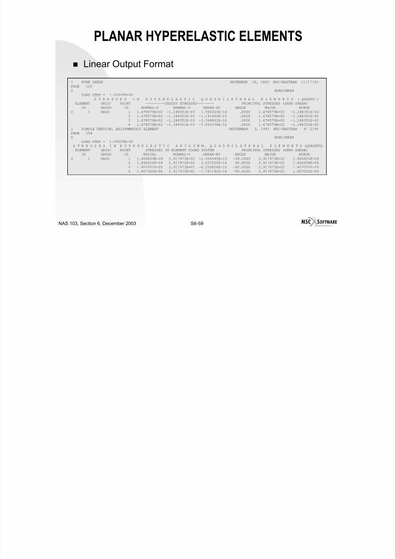
7/21/2019 Nonlinear Analysis Using MSC.nastran
http://slidepdf.com/reader/full/nonlinear-analysis-using-mscnastran 356/783
S6-58NAS 103, Section 6, December 2003
PLANAR HYPERELASTIC ELEMENTS
Linear Output Format
1 PURE SHEAR NOVEMBER 18, 1993 MSC/NASTRAN 11/17/93
PAGE 1250 NONLINEAR
LOAD STEP = 1.00000E+00
S T R E S S E S I N H Y P E R E L A S T I C Q U A D R I L A T E R A L E L E M E N T S ( QUADFD )ELEMENT GRID/ POINT ---------CAUCHY STRESSES-------- PRINCIPAL STRESSES (ZERO SHEAR)
ID GAUSS ID NORMAL-X NORMAL-Y SHEAR-XY ANGLE MAJOR MINOR0 1 GAUS 1 1.678579E+02 -1.188351E-03 1.560323E-16 .0000 1.678579E+02 -1.188351E-03
2 1.678579E+02 -1.188351E-03 -1.191492E-15 .0000 1.678579E+02 -1.188351E-033 1.678579E+02 -1.188351E-03 -3.368891E-16 .0000 1.678579E+02 -1.188351E-03
4 1.678579E+02 -1.188351E-03 -7.083336E-16 .0000 1.678579E+02 -1.188351E-031 SIMPLE TENSION, AXISYMMETRIC ELEMENT SEPTEMBER 3, 1993 MSC/NASTRAN 9/ 2/93PAGE 154
0 NONLINEARLOAD STEP = 1.00000E+00
S T R E S S E S I N H Y P E R E L A S T I C A X I S Y M M. Q U A D R I L A T E R A L E L E M E N T S (QUADXFD)ELEMENT GRID/ POINT STRESSES IN ELEMENT COORD SYSTEM PRINCIPAL STRESSES (ZERO SHEAR)
ID GAUSS ID RADIAL NORMAL-Y SHEAR-RY ANGLE MAJOR MINOR
0 1 GAUS 1 1.806839E-09 2.917973E+02 -1.456493E-15 -90.0000 2.917973E+02 1.806825E-092 1.806910E-09 2.917973E+02 3.027552E-16 90.0000 2.917973E+02 1.806939E-09
3 1.807052E-09 2.917973E+02 -6.255834E-15 -90.0000 2.917973E+02 1.807052E-094 1.807052E-09 2.917973E+02 -7.787191E-16 -90.0000 2.917973E+02 1.807052E-09

7/21/2019 Nonlinear Analysis Using MSC.nastran
http://slidepdf.com/reader/full/nonlinear-analysis-using-mscnastran 357/783
S6-59NAS 103, Section 6, December 2003
SOLID HYPERELASTIC ELEMENTS
HEXA, PENTA, and TETRA.
Properties are specified by PLSOLID. PLSOLID Bulk Data Entry
Defines a finite deformation solid element.
Format:
Example:
MIDPIDPLSOLID
10987654321
2120PLSOLID
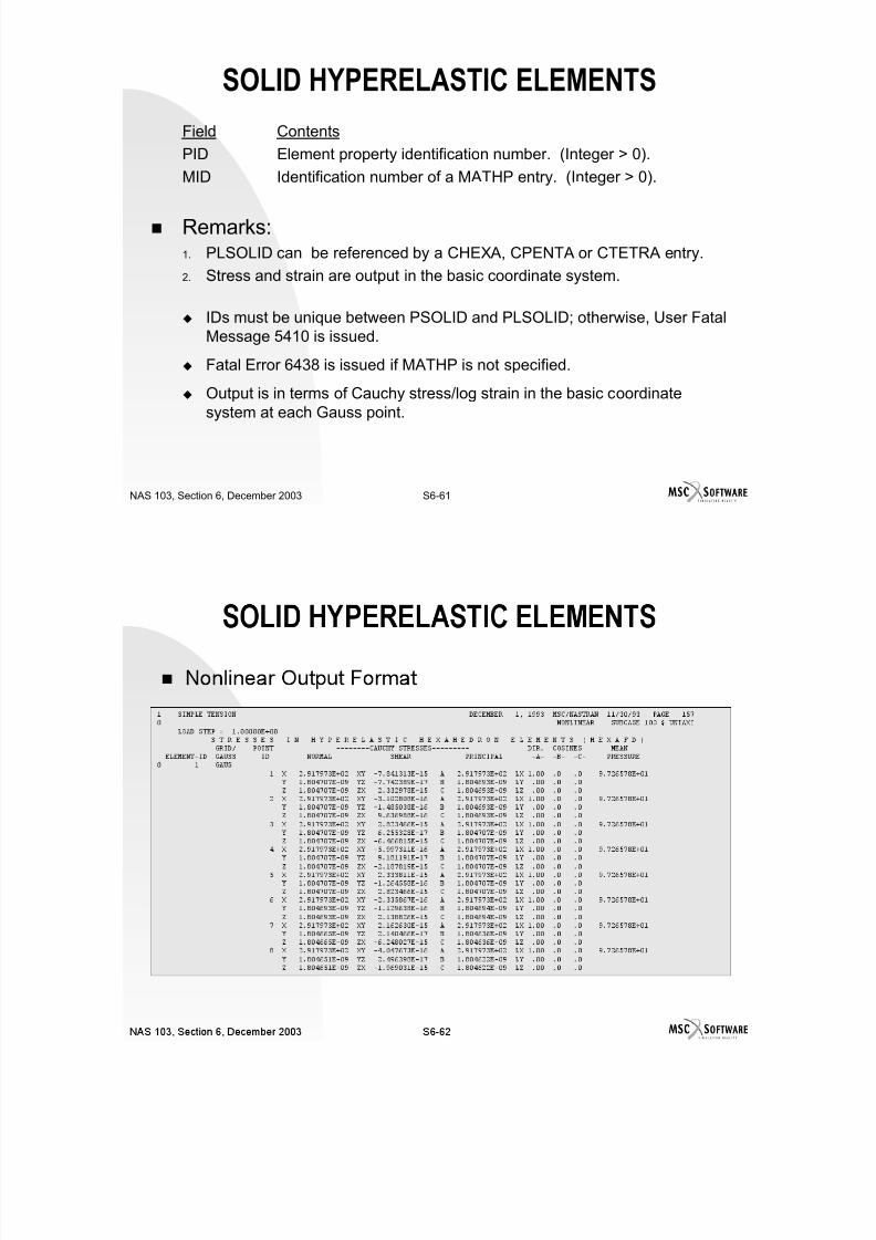
7/21/2019 Nonlinear Analysis Using MSC.nastran
http://slidepdf.com/reader/full/nonlinear-analysis-using-mscnastran 358/783
S6-60NAS 103, Section 6, December 2003
SOLID HYPERELASTIC ELEMENTSField Contents
PID Element property identification number. (Integer > 0).
MID Identification number of a MATHP entry. (Integer > 0).
Remarks:1. PLSOLID can be referenced by a CHEXA, CPENTA or CTETRA entry.
2. Stress and strain are output in the basic coordinate system.
IDs must be unique between PSOLID and PLSOLID; otherwise, User FatalMessage 5410 is issued.
Fatal Error 6438 is issued if MATHP is not specified. Output is in terms of Cauchy stress/log strain in the basic coordinate
system at each Gauss point.
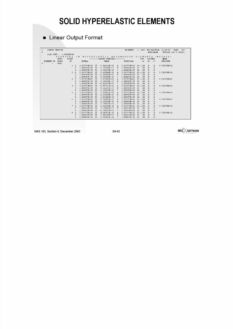
7/21/2019 Nonlinear Analysis Using MSC.nastran
http://slidepdf.com/reader/full/nonlinear-analysis-using-mscnastran 359/783
S6-61NAS 103, Section 6, December 2003

7/21/2019 Nonlinear Analysis Using MSC.nastran
http://slidepdf.com/reader/full/nonlinear-analysis-using-mscnastran 360/783

7/21/2019 Nonlinear Analysis Using MSC.nastran
http://slidepdf.com/reader/full/nonlinear-analysis-using-mscnastran 361/783
CONTACT (INTERFACE) ELEMENTS GAP
3-D slideline

7/21/2019 Nonlinear Analysis Using MSC.nastran
http://slidepdf.com/reader/full/nonlinear-analysis-using-mscnastran 362/783
S6-64NAS 103, Section 6, December 2003
GAP ELEMENT
Connects two grid points with the orientation (gapdirection).
Opening or closing (contact) is determined in the gapdirection.
Uses hard surface contact, i.e., no penetration of grid
points is allowed in the gap direction. Can specify friction between the two points.
Uses the penalty method for both contact and friction.
Can have a large opening between the two points. No large relative slipping between the two points is
permitted.
No large rotation for the two points (relative or rigid).

7/21/2019 Nonlinear Analysis Using MSC.nastran
http://slidepdf.com/reader/full/nonlinear-analysis-using-mscnastran 363/783
S6-65NAS 103, Section 6, December 2003
GAP ELEMENT
CGAP Bulk Data Entry Defines a gap or frictional element for nonlinear analysis.
Format:
Example:
Alternate Format and Example:
NoPGAPCGAP
Geometric
Nonlinearity
MaterialPropertyConnectivity
CIDX3X2X1GBGAPIDEIDCGAP
10987654321
-6.10.35.2112110217CGAP
CIDGOGAGAPIDEIDCGAP
13112110217CGAP
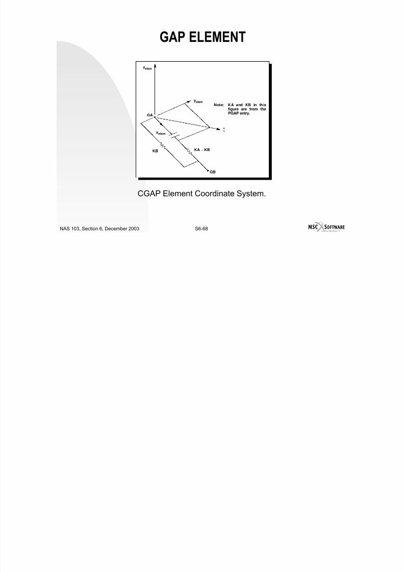
7/21/2019 Nonlinear Analysis Using MSC.nastran
http://slidepdf.com/reader/full/nonlinear-analysis-using-mscnastran 364/783
S6-66NAS 103, Section 6, December 2003
S6 67NAS 103 S ti 6 D b 2003
GAP ELEMENT CID identifies the element coordinate system.
T1, T2, and T3 of CID are the element x-, y-, and z-axis, respectively.
For noncoincident grid points GA and GB if CID is not defined GA - GB defines the x-axis.
Orientation vector is given by x1, x2, and x3, (like beam element) or GA -GO defines the x-y plane.
For coincident grid points GA and GB, If CID is blank, the job is terminated with a fatal message.

7/21/2019 Nonlinear Analysis Using MSC.nastran
http://slidepdf.com/reader/full/nonlinear-analysis-using-mscnastran 365/783
S6-67NAS 103, Section 6, December 2003
S6 68NAS 103 Section 6 December 2003
GAP ELEMENT
CGAP Element Coordinate System.
GA
GB
KA − KBKB
Note: KA and KB in thisfigure are from thePGAP entry.
v
zelem
yelem
xelem
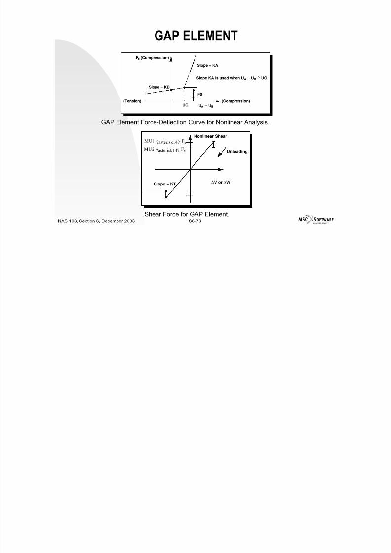
7/21/2019 Nonlinear Analysis Using MSC.nastran
http://slidepdf.com/reader/full/nonlinear-analysis-using-mscnastran 366/783
S6-68NAS 103, Section 6, December 2003
S6 69NAS 103 Section 6 December 2003
GAP ELEMENT
PGAP Bulk Data Entry Defines the properties of the gap element (CGAP entry).
Format:
Example:
0.250.251.0E+61.0E+62.50.0252PGAP
TRMINMARTMAX
MU2MU1KTKBKAF0U0PIDPGAP
10987654321
7/21/2019 Nonlinear Analysis Using MSC.nastran
http://slidepdf.com/reader/full/nonlinear-analysis-using-mscnastran 367/783
S6-69NAS 103, Section 6, December 2003
S6-70NAS 103 Section 6 December 2003
GAP ELEMENT
Shear Force for GAP Element.
F0
Fx (Compression)
Slope = KB
Slope = KA
(Tension)
Slope KA is used when UA – U
B ≥ UO
(Compression)UA – UBUO
Nonlinear Shear
Unloading
Slope = KT
MU1 ?asterisk14? Fx
MU2 ?asterisk14? Fx
∆V or ∆W
GAP Element Force-Deflection Curve for Nonlinear Analysis.

7/21/2019 Nonlinear Analysis Using MSC.nastran
http://slidepdf.com/reader/full/nonlinear-analysis-using-mscnastran 368/783
S6-70NAS 103, Section 6, December 2003
S6-71NAS 103, Section 6, December 2003
GAP ELEMENT There are two kinds of GAP element:
New and adaptive (TMAX >=0., preferred choice). New GAP can forcebisection and stiffness updates.
Old and non-adaptive (TMAX = –1.0).
New GAP element is recommended.
Old GAP element will not be covered.
Initial GAP opening is defined by U0, not by the distance.
Preload is defined by F0 (not recommended). Closed stiffness Ka is used when U A – UB ≥ U0.
The default for open stiffness Kb = 10 –14 Ka.
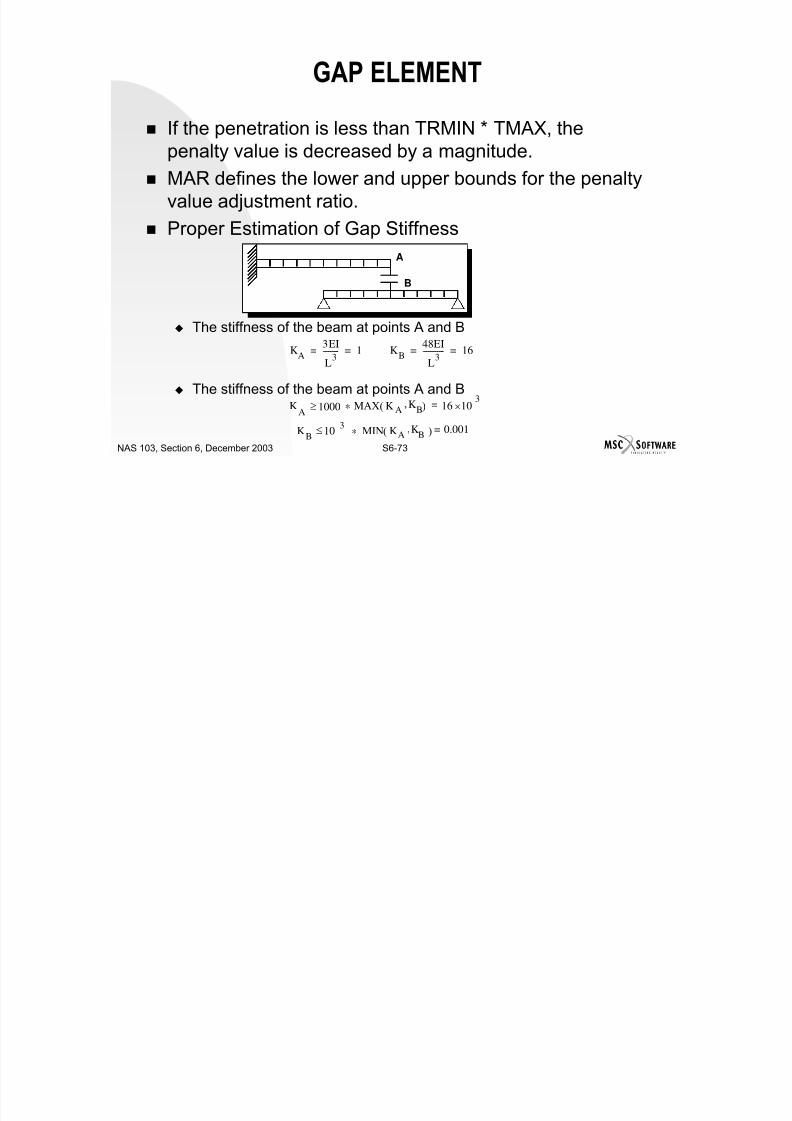
7/21/2019 Nonlinear Analysis Using MSC.nastran
http://slidepdf.com/reader/full/nonlinear-analysis-using-mscnastran 369/783
S6 71NAS 103, Section 6, December 2003
S6-72NAS 103, Section 6, December 2003
GAP ELEMENT
The transverse shear stiffness KT becomes active uponcontact. (The default = µ
1
* Ka
).
The continuation line is applicable for adaptive features
of the new GAP element only. Adaptive features are specified by TMAX > 0.
Penalty values are adjusted based on the penetration.
If the penetration is greater than TMAX, the penaltyvalue is increased by a magnitude.
New Default
1 Static Friction 0.0
2 Kinetic Friction 1

7/21/2019 Nonlinear Analysis Using MSC.nastran
http://slidepdf.com/reader/full/nonlinear-analysis-using-mscnastran 370/783
, ,
S6-73NAS 103, Section 6, December 2003
GAP ELEMENT
If the penetration is less than TRMIN * TMAX, thepenalty value is decreased by a magnitude.
MAR defines the lower and upper bounds for the penaltyvalue adjustment ratio.
Proper Estimation of Gap Stiffness
The stiffness of the beam at points A and B
The stiffness of the beam at points A and B
A
B
KA
3EI
L3
--------- 1= = KB
48EI
L3
------------ 16= =
KA
1000 * MAX K AK
B,( ) 16 10
3×=≥
KB
103–
* MIN KAK
B,( ) 0.001=≤

7/21/2019 Nonlinear Analysis Using MSC.nastran
http://slidepdf.com/reader/full/nonlinear-analysis-using-mscnastran 371/783
S6-74NAS 103, Section 6, December 2003
GAP ELEMENT The recommended stiffness acts rigid when closed and acts free when
open with an error of 0.1%.
Factors (103 or 10 –3) may be reduced to facilitate convergence at theexpense of accuracy.
Recommended stiffnesses are based on the decoupled stiffnesses.
Friction Features Friction effect is turned off with Kt = 0. Static and kinetic frictions are allowed.
Frictional gap problem is path dependent.
Sticking with elastic stiffness Kt before slipping.
Slipping is similar to plasticity. Sub-incremental process similar to plasticity is used for the new gap.
No sub-incremental process for the old gap.
Accuracy deteriorates if the increment produces large changes in thedisplacements with friction.

7/21/2019 Nonlinear Analysis Using MSC.nastran
http://slidepdf.com/reader/full/nonlinear-analysis-using-mscnastran 372/783
S6-75NAS 103, Section 6, December 2003
GAP ELEMENT
The slip locus is generalized by an ellipse:.
Fy2
Fz2
µsFx( )2
≤+ Closed and Sticking
Fy
2F
z
2µ
k F
x( )
2>+ Closed and Slipping

7/21/2019 Nonlinear Analysis Using MSC.nastran
http://slidepdf.com/reader/full/nonlinear-analysis-using-mscnastran 373/783
S6-76NAS 103, Section 6, December 2003
GAP ELEMENT
Caution for Using GAP Element Large rotation capability is not implemented.
When used for linear analysis, GAP stays linear with the initial stiffness.
The penalty values (Ka and Kt) should be as small as possible forsolution efficiency, but large enough for acceptable accuracy.
Penalty values are constants while the structural stiffness in the
adjacent structure changes continuously during loading. Avoid friction unless its effect is significant.
Use smaller increments if friction is involved.
Avoid complications by using isotropic friction (for old gap).
Typical coefficients of friction: Steel on steel (dry) 0.4 to 0.6
Steel on steel (greasy) 0.05 to 0.1
Brake lining on cast iron 0.3 to 0.4
Tire on pavement (dry) 0.8 to 0.9
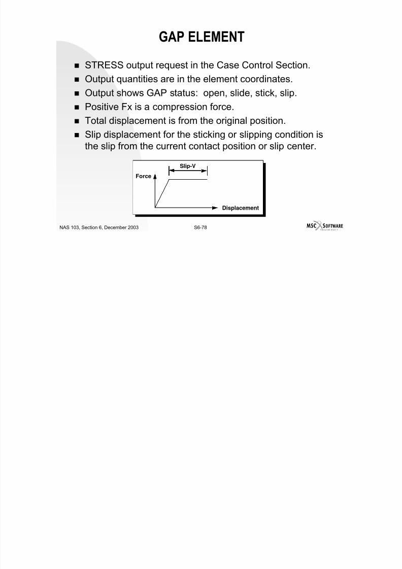
7/21/2019 Nonlinear Analysis Using MSC.nastran
http://slidepdf.com/reader/full/nonlinear-analysis-using-mscnastran 374/783
S6-77NAS 103, Section 6, December 2003
GAP ELEMENT
Output Format
1 NONLINEAR STATIC CONTACT OF A SPHERE ON A RIGID NG6603 JANUARY 26, 1993 MSC/NASTRAN 1/25/93 PAGE 353
FLAT PLANE. LOAD IN THE -Z IS 60. WITH FRICTION0 RESULTS ARE FOR A HEXA MODEL SUBCASE 3
LOAD STEP = 3.00000E+00S T R E S S E S ( F O R C E S ) I N G A P E L E M E N T S ( C G A P )
ELEMENT - F O R C E S I N E L E M S Y S T - - D I S P L A C E M E N T S I N E L E M S Y S T -
ID COMP-X SHEAR-Y SHEAR-Z AXIAL-U TOTAL-V TOTAL-W SLIP-V SLIP-W STATUS2001 5.41107E+00 -3.66852E-01 .0 2.20054E-02 -1.81889E-03 .0 -1.81522E-03 .0 STICK2002 1.03702E+01 -2.07404E+00 -1.66861E-14 1.97010E-01 -1.78610E-02 -6.96423E-19 -1.78403E-02 -5.29562E-19 SLIP2003 -1.21279E-09 .0 .0 4.20721E-01 -1.52148E-02 .0 -1.52148E-02 .0 OPEN
2004 5.23067E+00 .0 .0 2.20193E-02 -1.80472E-02 .0 -1.80472E-02 .0 SLIDE

7/21/2019 Nonlinear Analysis Using MSC.nastran
http://slidepdf.com/reader/full/nonlinear-analysis-using-mscnastran 375/783
S6-78NAS 103, Section 6, December 2003
GAP ELEMENT
STRESS output request in the Case Control Section.
Output quantities are in the element coordinates. Output shows GAP status: open, slide, stick, slip.
Positive Fx is a compression force.
Total displacement is from the original position.
Slip displacement for the sticking or slipping condition isthe slip from the current contact position or slip center.
Slip-V
Force
Displacement
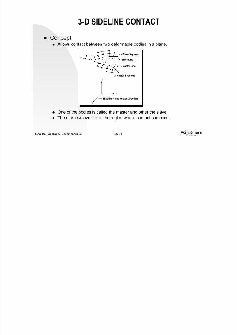
7/21/2019 Nonlinear Analysis Using MSC.nastran
http://slidepdf.com/reader/full/nonlinear-analysis-using-mscnastran 376/783
S6-79NAS 103, Section 6, December 2003
GAP ELEMENT
Slip displacement for the open or sliding condition is thesame as the total displacement.
If open , ( µ = 0 or µ ≠ 0 ), Total-V = Slip-V.
If sliding, Total-V = Slip-V ≠ 0 for new gap.
If sticking, Slip-V ≠ Total-V ≠ 0.
If slipped, Total-V ≠ Slip-V = Vs from slip center.

7/21/2019 Nonlinear Analysis Using MSC.nastran
http://slidepdf.com/reader/full/nonlinear-analysis-using-mscnastran 377/783

7/21/2019 Nonlinear Analysis Using MSC.nastran
http://slidepdf.com/reader/full/nonlinear-analysis-using-mscnastran 378/783
S6-81NAS 103, Section 6, December 2003
3-D SIDELINE CONTACT A master/slave segment is the line joining two consecutive nodes.
Master/slave nodes are the grid points in the contact region.
The slideline plane is the plane in which the master and slave nodesmust lie.
The master and slave nodes can have large relative motion within theslideline plane.
Relative motions outside the slideline plane are ignored. Therefore,they must be small.
Contact is determined between the slave nodes and the master line(very important).

7/21/2019 Nonlinear Analysis Using MSC.nastran
http://slidepdf.com/reader/full/nonlinear-analysis-using-mscnastran 379/783
S6-82NAS 103, Section 6, December 2003
3-D SIDELINE CONTACT 3-D Slideline Element
Consists of three nodes: slave, master node 1, and master node 2.
where S, m1, m2 = slave, master node 1 and master node 2, respectivelya, a0 = current and previous surface coordinate
gn = penetration of slave node into the master segment
gt = sliding of the slave node on the master segment
n = normal direction for the master segment
x2 x 1–6
5
1
4 3
n
St
m1
gn
gt
x2 x 1–
x2 x1–
a
a0
m2
2

7/21/2019 Nonlinear Analysis Using MSC.nastran
http://slidepdf.com/reader/full/nonlinear-analysis-using-mscnastran 380/783

7/21/2019 Nonlinear Analysis Using MSC.nastran
http://slidepdf.com/reader/full/nonlinear-analysis-using-mscnastran 381/783
S6-84NAS 103, Section 6, December 2003
3-D SIDELINE CONTACT Note that the master nodes to which a slave node connects change
continually.
The only way an internal element can be identified is by the external gridnumber of the slave node.

7/21/2019 Nonlinear Analysis Using MSC.nastran
http://slidepdf.com/reader/full/nonlinear-analysis-using-mscnastran 382/783
S6-85NAS 103, Section 6, December 2003
3-D SIDELINE CONTACT Output
1 NONLINEAR STATIC CONTACT OF A SPHERE ON A RIGID PLANE WITHOUT FRIC JANUARY 26, 1993 MSC/NASTRAN 1/25/93 PAGE53
0 SUBCASE 3LOAD STEP = 3.00000E+00
R E S U L T S F O R S L I D E L I N E E L E M E N T S (IN ELEMENT SYSTEM)
SLAVE CONTAC MASTER SURFACE NORMAL SHEAR NORMAL SHEAR NORMAL SLIP SLIP SLIP
GRID ID GRID1 GRID2 CORDINATE FORCE FORCE STRESS STRESS GAP RATIO CODE110 1 315 313 3.5261E-01 1.1142E+01 .0 1.8074E+01 .0 6.6289E-03 -4.7546E-02 .0 SLIDE
108 1 315 313 2.2509E-01 9.9720E+00 .0 1.6162E+01 .0 5.8047E-03 -3.5960E-02 .0 SLIDE105 1 315 313 1.0759E-01 5.3024E+00 .0 1.7893E+01 .0 1.9600E-03 -1.8563E-02 .0 SLIDE208 2 315 314 1.0000E+00 .0 .0 .0 .0 -1.1209E+00 .0 .0 OPEN
176 2 315 314 4.7187E-01 2.7194E+00 .0 4.5926E+00 .0 1.5293E-03 -3.9368E-02 .0 SLIDE170 2 315 314 1.0759E-01 5.2982E+00 .0 1.7879E+01 .0 1.9684E-03 -1.8563E-02 .0 SLIDE

7/21/2019 Nonlinear Analysis Using MSC.nastran
http://slidepdf.com/reader/full/nonlinear-analysis-using-mscnastran 383/783
S6-86NAS 103, Section 6, December 2003
3-D SIDELINE CONTACT General Features
Can have as many slideline contact regions as desired.
Contact is determined only for slave nodes and the master line. May specify symmetric penetration, i.e., contact is determined for both
slave and master nodes into master and slave line, respectively.
Initial penetration of slave nodes into master line is not allowed.
User Warning Message 6315 is issued, if the initial penetration is lessthan 10% of the master segment length.
Coordinates of the slave node are changed internally to precludepenetration.
User Fatal Message 6314 is issued, if initial penetration for any slavenode is greater then 10% of the master segment length.
The master and slave nodes must be in the slideline plane in the initialgeometry; otherwise, Fatal Message 6312 is issued.

7/21/2019 Nonlinear Analysis Using MSC.nastran
http://slidepdf.com/reader/full/nonlinear-analysis-using-mscnastran 384/783
S6-87NAS 103, Section 6, December 2003
3-D SIDELINE CONTACT During the analysis, no check is made to ensure that the master and
slave nodes are in the slideline plane.
The slave or master nodes need not be attached to the physical element(model rigid surface).
Ensure that the contact region is properly defined so that there are noerroneous overhangs.
Forces/stresses are associated with slave nodes.
Output can be requested in SORT1 or SORT2. There is only one output format.

7/21/2019 Nonlinear Analysis Using MSC.nastran
http://slidepdf.com/reader/full/nonlinear-analysis-using-mscnastran 385/783
S6-88NAS 103, Section 6, December 2003
3-D SIDELINE CONTACT User Interface
Bulk Data entries: BCONP Defines the parameters for a contact region and its
properties.
BLSEG Defines the grid points on the master/slave line.
BFRIC Defines the frictional properties.
BWIDTH Defines the width/thickness associated with each slave
node. BOUTPUT Defines the output requests for slave nodes in a slideline
contact region.
Case Control command: BOUTPUT Selects contact region for output
DMAP parameter: ADPCON Adjusts penalty values on restart.

7/21/2019 Nonlinear Analysis Using MSC.nastran
http://slidepdf.com/reader/full/nonlinear-analysis-using-mscnastran 386/783
S6-89NAS 103, Section 6, December 2003
BCONP BULK DATA ENTRY Description:
Defines the parameters for a contact region and its properties
Format:
Example:
Field ContentsID Contact region identification number (Integer > 0)SLAVE Slave region identification number (Integer > 0).
MASTER Master region identification number (Integer > 0)
SFAC Stiffness scaling factor. This factor is used to scale thepenalty values automatically calculated by the program. (Real> 0 or blank)
1331151095BCOMP
CIDPTYPEFRICIDSFACMASTERSLAVEIDBCONP
10987654321

7/21/2019 Nonlinear Analysis Using MSC.nastran
http://slidepdf.com/reader/full/nonlinear-analysis-using-mscnastran 387/783
S6-90NAS 103, Section 6, December 2003
BCONP BULK DATA ENTRYField Contents
FRICID Contact friction identification number (Integer > 0 or blank)
PTYPE Penetration type (Integer = 1 or 2; Default =1).1: unsymmetrical (slave penetration only) (default)
2: symmetrical
CID Coordinate system ID to define the slide line plane vector andthe slide line plane of contact. (Integer > 0 or blank; Default =0 which means the basic coordinate system)

7/21/2019 Nonlinear Analysis Using MSC.nastran
http://slidepdf.com/reader/full/nonlinear-analysis-using-mscnastran 388/783
S6-91NAS 103, Section 6, December 2003
BCONP BULK DATA ENTRY
Can have as many contact regions as desired. Penalty values are automatically selected based on the diagonal terms
of grid points. In symmetrical penetration, both the slave and master nodes are
checked for penetration into the master and slave surface, respectively. The t3 direction of CID is the z-direction of all the 3-D slideline elements
(one corresponding to each slave node and also to each master nodefor symmetric penetration) of the contact region.
kSlave Line
Slideline Plane Vector Direction
Master Line
x
y
z
k-1th Slave Segment
1-th Master Segment
k − 1k + 1
l + 1
l − 1

7/21/2019 Nonlinear Analysis Using MSC.nastran
http://slidepdf.com/reader/full/nonlinear-analysis-using-mscnastran 389/783
S6-92NAS 103, Section 6, December 2003
BLSEG BULK DATA ENTRY Description:
Defines a curve which consists of a number of line segments via grid
numbers that may come in contact with other body. A line segment isdefined between every two consecutive grid points. Thus, number of linesegments defined is equal to the number of grid points specified minus1. A corresponding BWlDTH Bulk data entry may be required to definethe width/thickness of each line segment. If the corresponding BWlDTH
is not present, the width/thickness for each line segment is assumedunity
Format:
G12G11
G10BYG9THRUG8
G7G6G5G4G3G2G1IDBLSEG
10987654321

7/21/2019 Nonlinear Analysis Using MSC.nastran
http://slidepdf.com/reader/full/nonlinear-analysis-using-mscnastran 390/783
S6-93NAS 103, Section 6, December 2003
BLSEG BULK DATA ENTRY Examples:
Field Contents
ID Line segments identification number (Integer > 0)Gi Grid numbers on a curve in a continuous topological order so
that the normal to the segment points towards other curve.
Grid points must be specified in topological order.
Normals (z × t) of the master segments must face toward the slave linefor unsymmetric penetration.
Normals of master and slave segments must face each other forsymmetric penetration
44THRU35
33323027
14BY21THRU515BLSEG

7/21/2019 Nonlinear Analysis Using MSC.nastran
http://slidepdf.com/reader/full/nonlinear-analysis-using-mscnastran 391/783
S6-94NAS 103, Section 6, December 2003
BLSEG BULK DATA ENTRY These conditions are accomplished by traversing counterclockwise or
clockwise from the master line to the slave line depending on whetherthe slideline vector forms the right-hand rule or the left-hand rule.
The master line must have at least two grid points.
The slave line may have only one grid point for unsymmetricalpenetration.
Two grid points in a line cannot be the same or coincident except for the
first point and the last point, which signify a close region.

7/21/2019 Nonlinear Analysis Using MSC.nastran
http://slidepdf.com/reader/full/nonlinear-analysis-using-mscnastran 392/783
S6-95NAS 103, Section 6, December 2003
BFRIC BULK DATA ENTRY Description:
Defines frictional properties between two bodies in contact.
Format:
Example:
Field ContentsFID Friction identification number (Integer > 0)FSTIF Frictional stiffness in stick (Real > 0.0). Default =
automatically selected by the program.MU1 Coefficient of static friction (Real > 0.0).
(Note that no distinction is made between static and kinetic friction.)
MU1FSTIFFIDBFRIC
10987654321
0.333BFRIC

7/21/2019 Nonlinear Analysis Using MSC.nastran
http://slidepdf.com/reader/full/nonlinear-analysis-using-mscnastran 393/783
S6-96NAS 103, Section 6, December 2003
BWIDTH BULK DATA ENTRY Description
Defines width/thickness for line segments in 3-D/2-D slideline contact
defined in the corresponding BLSEG BULK Data entry. This entry maybe omitted if the width/thickness of each segment defined in the BLSEGentry is unity. Number of thicknesses to be specified is equal to thenumber of segments defined in the corresponding BLSEG entry. If there is no corresponding BLSEG entry, the width/thickness specified in
the entry are not used by the program. Format:
W12W11
W10BYW9THRUW8
W7W6W5W4W3W2W1IDBWIDTH
10987654321

7/21/2019 Nonlinear Analysis Using MSC.nastran
http://slidepdf.com/reader/full/nonlinear-analysis-using-mscnastran 394/783
S6-97NAS 103, Section 6, December 2003
BWIDTH BULK DATA ENTRY Examples:
Field Contents
ID Width/thickness set identification number (Real > 0.0).Wi Width/Thickness values for the corresponding line segments
defined in the BLSEG entry. (Real > 0.0).
44THRU35
2222
1BY5THRU215BWIDTH

7/21/2019 Nonlinear Analysis Using MSC.nastran
http://slidepdf.com/reader/full/nonlinear-analysis-using-mscnastran 395/783
S6-98NAS 103, Section 6, December 2003
BWIDTH BULK DATA ENTRY ID is the same as the slave line (BLSEG) ID.
Widths/thicknesses are specified for slave nodes only. Default = unity.
Widths/thicknesses are used for calculating contact stresses. Each slave node is assigned a contributory area.
The number of widths to be specified is equal to the number of slavenodes -1.
For only one slave node, specify the area in W1 field.

7/21/2019 Nonlinear Analysis Using MSC.nastran
http://slidepdf.com/reader/full/nonlinear-analysis-using-mscnastran 396/783
S6-99NAS 103, Section 6, December 2003
BOUTPUT BULK DATA ENTRY Description
Defines the slave nodes at which the output is requested.
Format:
Example:
Field ContentsID Boundary identification number for which output is desired
(Integer > 0.0).Gi Slave node numbers for which output is desired. Note: The ID is the same as the corresponding BCONP ID. This entry
can selectively specify the slave grid points for which OUTPUT isdesired.
B10BYG9THRUG8
G8G7G6G5G4G3G2G1
ALLIDBPOUTPUT
10987654321
ALL15BOUTPUT

7/21/2019 Nonlinear Analysis Using MSC.nastran
http://slidepdf.com/reader/full/nonlinear-analysis-using-mscnastran 397/783
S6-100NAS 103, Section 6, December 2003
BOUTPUT CASE CONTROL COMMAND Description:
Selects slave nodes specified in the Bulk Data entry BOUTPUT for
history output. Format:
Example: BOUTPUT = ALL BOUTPUT = 5
Field ContentsSORT1 Output is presented as a tabular listing of slave nodes for
each load or time depending on the solution sequence.SORT2 Output is presented as a tabular listing of load or time for
each slave node.
BOUTPUT
SORT1, PRINT
SORT2, PUNCH
PLOT ALL
n
None
=

7/21/2019 Nonlinear Analysis Using MSC.nastran
http://slidepdf.com/reader/full/nonlinear-analysis-using-mscnastran 398/783
S6-101NAS 103, Section 6, December 2003
BOUTPUT CASE CONTROL COMMANDField Contents
PRINT The print file (Fortran I/O unit 6) is the output media.
PUNCH The punch file is the output media.PLOT Generate slave node results history but do not print.
ALL Histories of all the slave nodes listed in all the BOUTPUTbulk data entries are output. If no BOUTPUT bulk data entriesare specified, histories of all the lave nodes in all the contact
regions are output.n Set identification of previously appearing set command. Only
contact regions whose identification numbers.
none Result histories for no slave nodes are output.
Note: This command selects the contact region for which output isdesired.

7/21/2019 Nonlinear Analysis Using MSC.nastran
http://slidepdf.com/reader/full/nonlinear-analysis-using-mscnastran 399/783
S6-102NAS 103, Section 6, December 2003
PARAM ADPCON User interface
PARAM,ADPCON,(real value)
On restart, ADPCON can be used to increase ordecrease the penalty values for all the line contactregions.
A negative value of ADPCON implies that penalty values
are calculated at the beginning of a subcase only. Thisis useful for contact between elastic bodies.
Penalty values for a line contact region are given by
where ks = number calculated automatically for a slave node by theprogram
SFAC = scale factor specified in BCONP
| ADPCON |* SFAC * k s
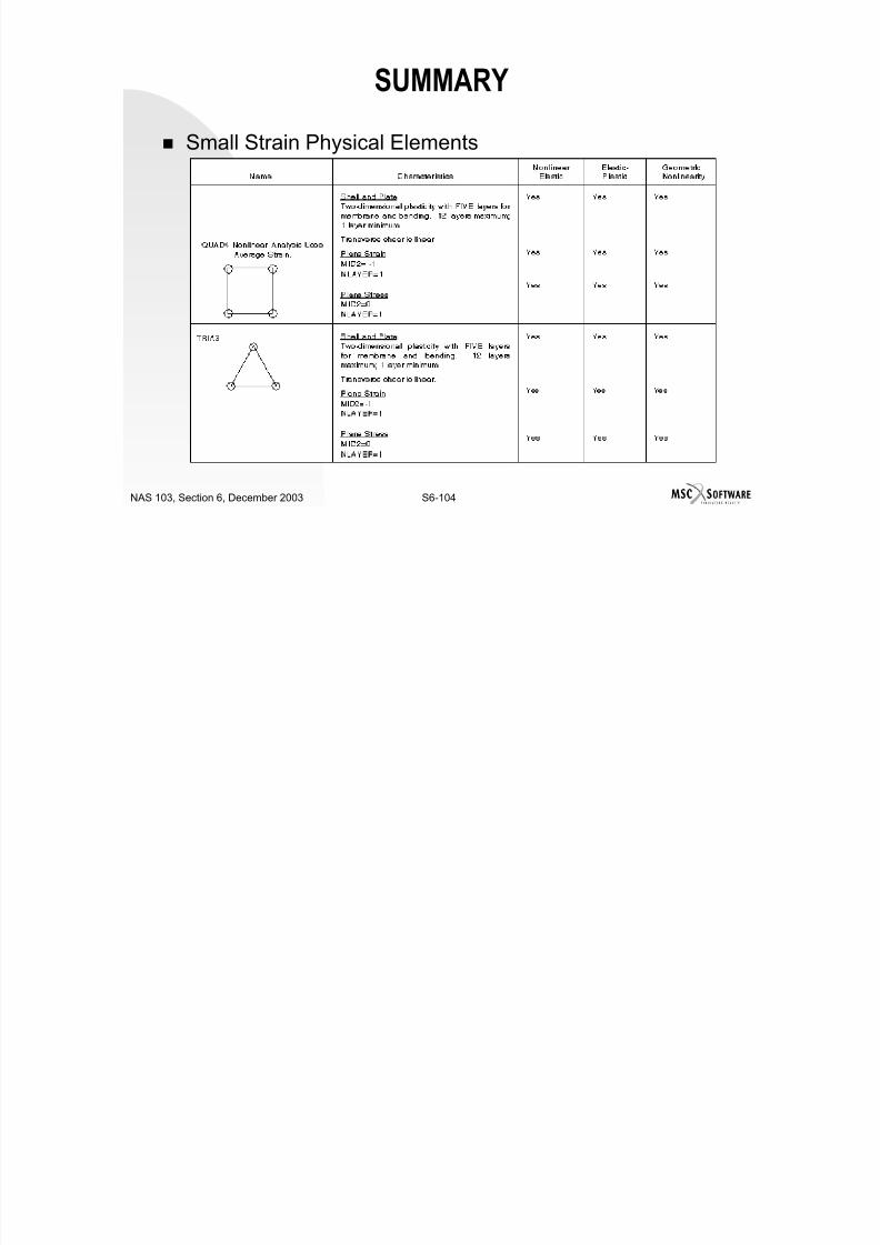
7/21/2019 Nonlinear Analysis Using MSC.nastran
http://slidepdf.com/reader/full/nonlinear-analysis-using-mscnastran 400/783
S6-103NAS 103, Section 6, December 2003
SUMMARY Small Strain Physical Elements
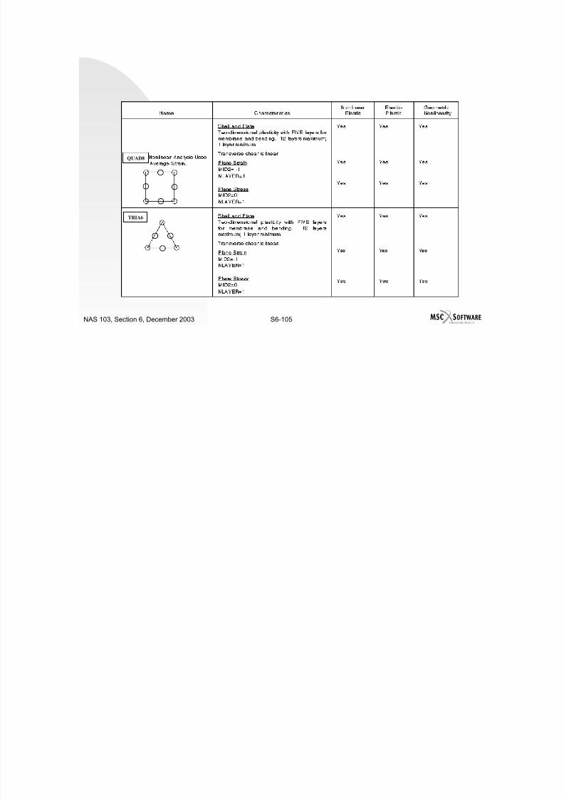
7/21/2019 Nonlinear Analysis Using MSC.nastran
http://slidepdf.com/reader/full/nonlinear-analysis-using-mscnastran 401/783
S6-104NAS 103, Section 6, December 2003
SUMMARY Small Strain Physical Elements

7/21/2019 Nonlinear Analysis Using MSC.nastran
http://slidepdf.com/reader/full/nonlinear-analysis-using-mscnastran 402/783
S6-105NAS 103, Section 6, December 2003
QUAD8
TRIA6

7/21/2019 Nonlinear Analysis Using MSC.nastran
http://slidepdf.com/reader/full/nonlinear-analysis-using-mscnastran 403/783
S6-106NAS 103, Section 6, December 2003
SUMMARY Small Strain Physical Elements

7/21/2019 Nonlinear Analysis Using MSC.nastran
http://slidepdf.com/reader/full/nonlinear-analysis-using-mscnastran 404/783
S6-107NAS 103, Section 6, December 2003
SUMMARY Small Strain Physical Elements (Cont.)
One-dimensional stress-strain curves use MAT1.
All other elements may be used for nonlinear analysis as long as theyremain linear.
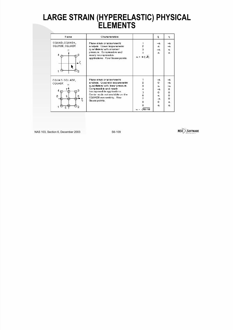
7/21/2019 Nonlinear Analysis Using MSC.nastran
http://slidepdf.com/reader/full/nonlinear-analysis-using-mscnastran 405/783
S6-108NAS 103, Section 6, December 2003
TETRA10
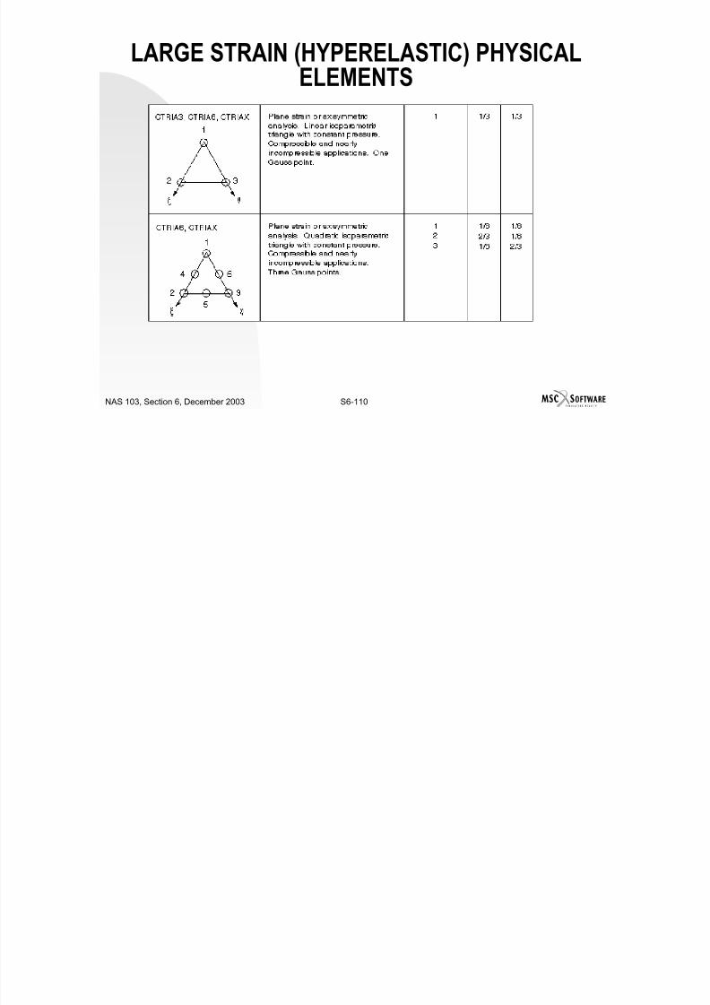
7/21/2019 Nonlinear Analysis Using MSC.nastran
http://slidepdf.com/reader/full/nonlinear-analysis-using-mscnastran 406/783
S6-109NAS 103, Section 6, December 2003
LARGE STRAIN (HYPERELASTIC) PHYSICAL
ELEMENTS

7/21/2019 Nonlinear Analysis Using MSC.nastran
http://slidepdf.com/reader/full/nonlinear-analysis-using-mscnastran 407/783
S6-110NAS 103, Section 6, December 2003
LARGE STRAIN (HYPERELASTIC) PHYSICAL
ELEMENTS
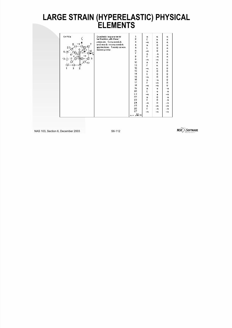
7/21/2019 Nonlinear Analysis Using MSC.nastran
http://slidepdf.com/reader/full/nonlinear-analysis-using-mscnastran 408/783
S6-111NAS 103, Section 6, December 2003
LARGE STRAIN (HYPERELASTIC) PHYSICAL
ELEMENTS

7/21/2019 Nonlinear Analysis Using MSC.nastran
http://slidepdf.com/reader/full/nonlinear-analysis-using-mscnastran 409/783
S6-112NAS 103, Section 6, December 2003
LARGE STRAIN (HYPERELASTIC) PHYSICAL
ELEMENTS
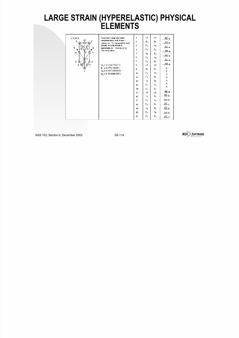
7/21/2019 Nonlinear Analysis Using MSC.nastran
http://slidepdf.com/reader/full/nonlinear-analysis-using-mscnastran 410/783
S6-113NAS 103, Section 6, December 2003
LARGE STRAIN (HYPERELASTIC) PHYSICAL
ELEMENTS
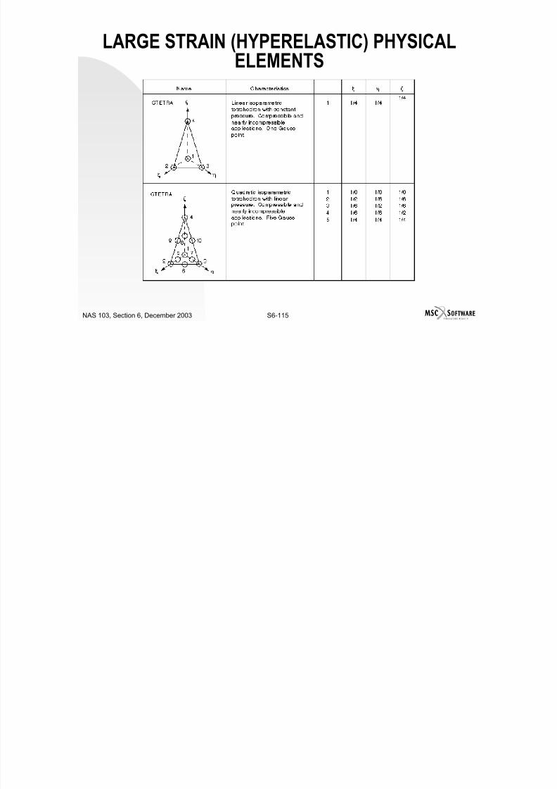
7/21/2019 Nonlinear Analysis Using MSC.nastran
http://slidepdf.com/reader/full/nonlinear-analysis-using-mscnastran 411/783
S6-114NAS 103, Section 6, December 2003
LARGE STRAIN (HYPERELASTIC) PHYSICAL
ELEMENTS
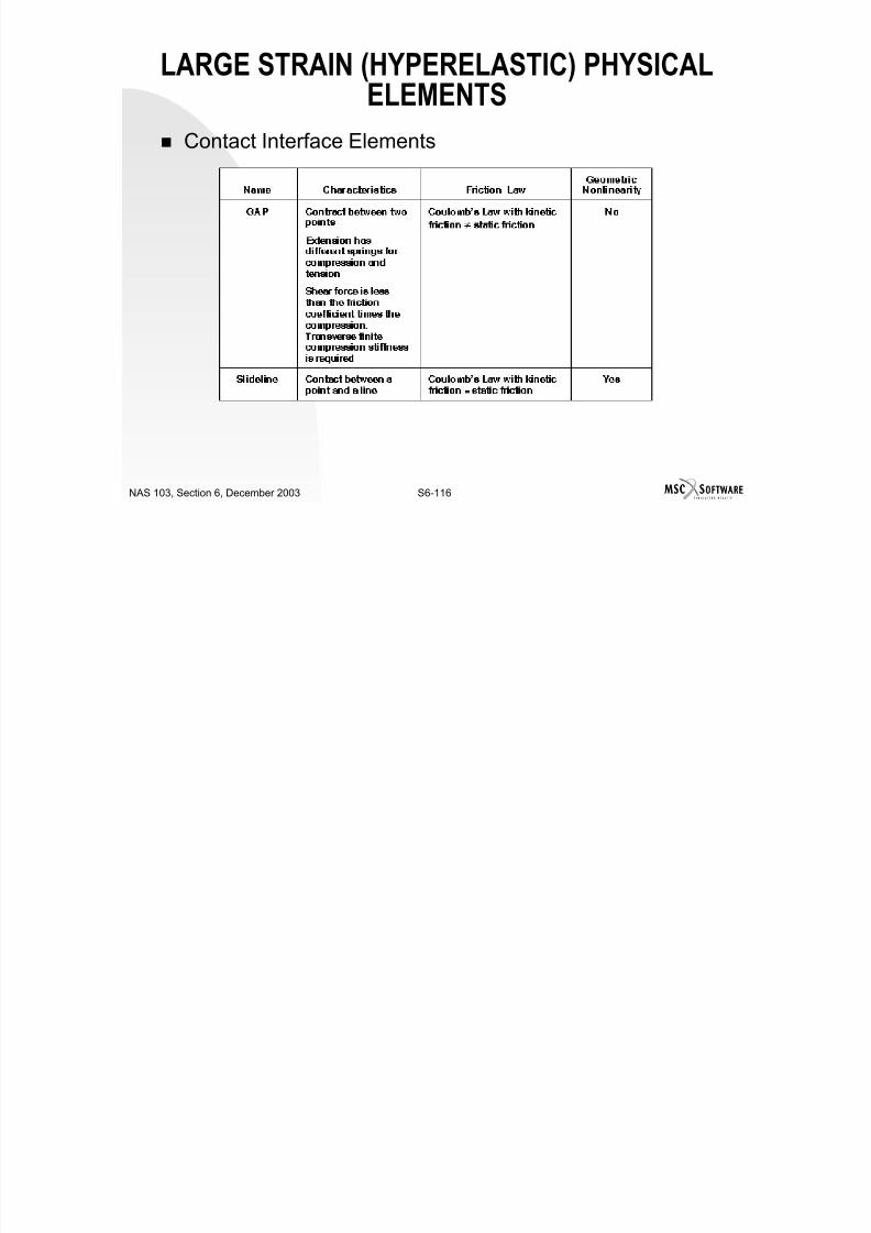
7/21/2019 Nonlinear Analysis Using MSC.nastran
http://slidepdf.com/reader/full/nonlinear-analysis-using-mscnastran 412/783
S6-115NAS 103, Section 6, December 2003
LARGE STRAIN (HYPERELASTIC) PHYSICAL
ELEMENTS
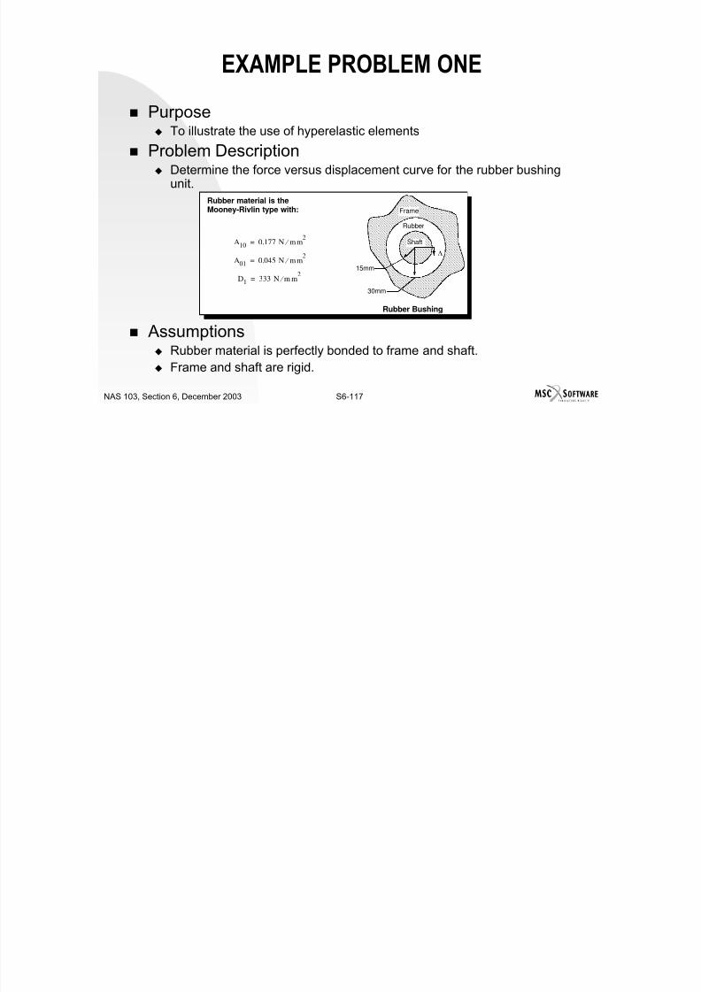
7/21/2019 Nonlinear Analysis Using MSC.nastran
http://slidepdf.com/reader/full/nonlinear-analysis-using-mscnastran 413/783
S6-116NAS 103, Section 6, December 2003
LARGE STRAIN (HYPERELASTIC) PHYSICAL
ELEMENTS Contact Interface Elements
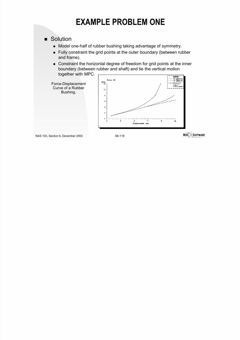
7/21/2019 Nonlinear Analysis Using MSC.nastran
http://slidepdf.com/reader/full/nonlinear-analysis-using-mscnastran 414/783
S6-117NAS 103, Section 6, December 2003
EXAMPLE PROBLEM ONE
Purpose To illustrate the use of hyperelastic elements
Problem Description Determine the force versus displacement curve for the rubber bushing
unit.
Assumptions Rubber material is perfectly bonded to frame and shaft. Frame and shaft are rigid.
Rubber
Frame
Shaft
15mm
30mm
Rubber material is theMooney-Rivlin type with:
Rubber Bushing
A10 0.177 N mm2
⁄ =
A01 0.045 N mm2
⁄ =
D1 333 N m m2
⁄ =
∆
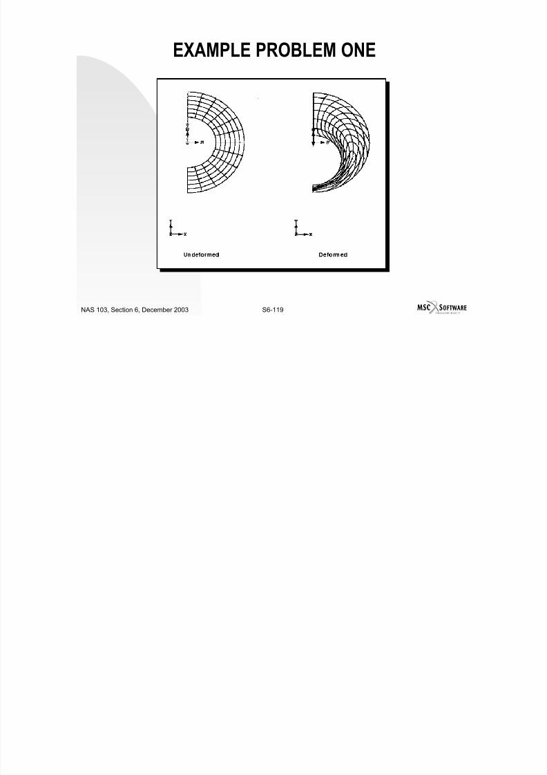
7/21/2019 Nonlinear Analysis Using MSC.nastran
http://slidepdf.com/reader/full/nonlinear-analysis-using-mscnastran 415/783
S6-118NAS 103, Section 6, December 2003
EXAMPLE PROBLEM ONE
Solution Model one-half of rubber bushing taking advantage of symmetry.
Fully constraint the grid points at the outer boundary (between rubberand frame).
Constraint the horizontal degree of freedom for grid points at the innerboundary (between rubber and shaft) and tie the vertical motiontogether with MPC.
Force-DisplacementCurve of a Rubber
Bushing.
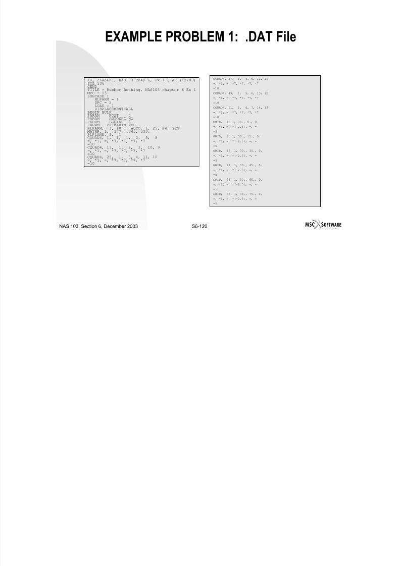
7/21/2019 Nonlinear Analysis Using MSC.nastran
http://slidepdf.com/reader/full/nonlinear-analysis-using-mscnastran 416/783
S6-119NAS 103, Section 6, December 2003
EXAMPLE PROBLEM ONE
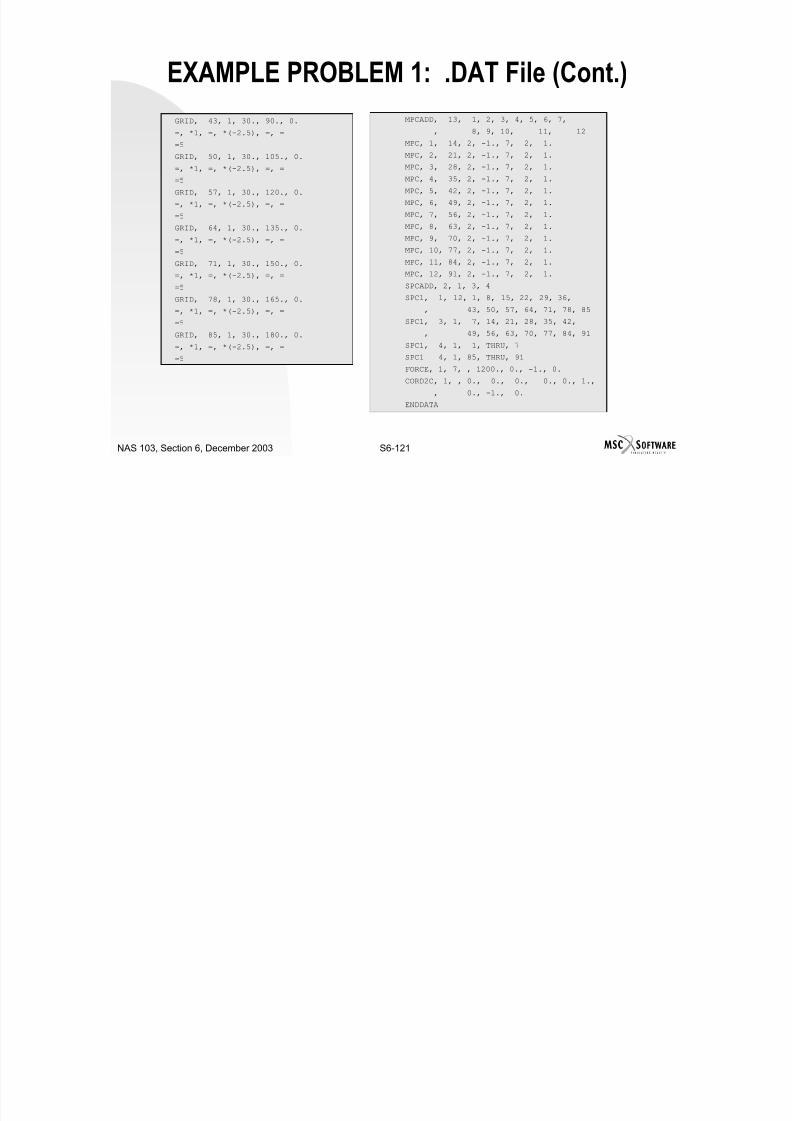
7/21/2019 Nonlinear Analysis Using MSC.nastran
http://slidepdf.com/reader/full/nonlinear-analysis-using-mscnastran 417/783
S6-120NAS 103, Section 6, December 2003
EXAMPLE PROBLEM 1: .DAT File
ID, chap6E1, NAS103 Chap 6, EX 1 $ AR (12/03)SOL 106
CENDTITLE = Rubber Bushing, NAS103 chapter 6 Ex 1MPC = 13SUBCASE 1
NLPARM = 1SPC = 2LOAD = 1DISPLACEMENT=ALL
BEGIN BULKPARAM POST 0PARAM AUTOSPC NOPARAM LGDISP 2PARAM PRTMAXIM YESNLPARM, 1, 10, , AUTO, 1, 25, PW, YES
MATHP, 1, .177, .045, 333.PLPLANE, 1, 1CQUAD4, 1, 1, 1, 2, 9, 8=, *1, =, *7, *7, *7, *7=10CQUAD4, 13, 1, 2, 3, 10, 9=, *1, =, *7, *7, *7, *7=10CQUAD4, 25, 1, 3, 4, 11, 10=, *1, =, *7, *7, *7, *7=10
CQUAD4, 37, 1, 4, 5, 12, 11
=, *1, =, *7, *7, *7, *7
=10
CQUAD4, 49, 1, 5, 6, 13, 12
=, *1, =, *7, *7, *7, *7
=10
CQUAD4, 61, 1, 6, 7, 14, 13
=, *1, =, *7, *7, *7, *7
=10
GRID, 1, 1, 30., 0., 0.
=, *1, =, *(-2.5), =, =
=5
GRID, 8, 1, 30., 15., 0.
=, *1, =, *(-2.5), =, =
=5
GRID, 15, 1, 30., 30., 0.
=, *1, =, *(-2.5), =, =
=5
GRID, 22, 1, 30., 45., 0.
=, *1, =, *(-2.5), =, =
=5
GRID, 29, 1, 30., 60., 0.
=, *1, =, *(-2.5), =, =
=5
GRID, 36, 1, 30., 75., 0.
=, *1, =, *(-2.5), =, =
=5

7/21/2019 Nonlinear Analysis Using MSC.nastran
http://slidepdf.com/reader/full/nonlinear-analysis-using-mscnastran 418/783
S6-121NAS 103, Section 6, December 2003
EXAMPLE PROBLEM 1: .DAT File (Cont.)
GRID, 43, 1, 30., 90., 0.
=, *1, =, *(-2.5), =, =
=5
GRID, 50, 1, 30., 105., 0.
=, *1, =, *(-2.5), =, =
=5
GRID, 57, 1, 30., 120., 0.
=, *1, =, *(-2.5), =, =
=5
GRID, 64, 1, 30., 135., 0.
=, *1, =, *(-2.5), =, =
=5
GRID, 71, 1, 30., 150., 0.
=, *1, =, *(-2.5), =, =
=5
GRID, 78, 1, 30., 165., 0.
=, *1, =, *(-2.5), =, =
=5
GRID, 85, 1, 30., 180., 0.
=, *1, =, *(-2.5), =, =
=5
MPCADD, 13, 1, 2, 3, 4, 5, 6, 7,
, 8, 9, 10, 11, 12
MPC, 1, 14, 2, -1., 7, 2, 1.
MPC, 2, 21, 2, -1., 7, 2, 1.
MPC, 3, 28, 2, -1., 7, 2, 1.
MPC, 4, 35, 2, -1., 7, 2, 1.
MPC, 5, 42, 2, -1., 7, 2, 1.
MPC, 6, 49, 2, -1., 7, 2, 1.
MPC, 7, 56, 2, -1., 7, 2, 1.
MPC, 8, 63, 2, -1., 7, 2, 1.
MPC, 9, 70, 2, -1., 7, 2, 1.
MPC, 10, 77, 2, -1., 7, 2, 1.
MPC, 11, 84, 2, -1., 7, 2, 1.
MPC, 12, 91, 2, -1., 7, 2, 1.
SPCADD, 2, 1, 3, 4
SPC1, 1, 12, 1, 8, 15, 22, 29, 36,
, 43, 50, 57, 64, 71, 78, 85
SPC1, 3, 1, 7, 14, 21, 28, 35, 42,
, 49, 56, 63, 70, 77, 84, 91
SPC1, 4, 1, 1, THRU, 7SPC1 4, 1, 85, THRU, 91
FORCE, 1, 7, , 1200., 0., -1., 0.
CORD2C, 1, , 0., 0., 0., 0., 0., 1.,
, 0., -1., 0.
ENDDATA

7/21/2019 Nonlinear Analysis Using MSC.nastran
http://slidepdf.com/reader/full/nonlinear-analysis-using-mscnastran 419/783
S6-122NAS 103, Section 6, December 2003
EXAMPLE PROBLEM TWO
Purpose To illustrate the use of axisymmetric hyperelastic elements and follower
forces.
Problem Description A circular plate is 15 inches in diameter and 0.5 inches thick. It is simply
supported along the edge and is subjected to a uniform pressure of 45psi. Plot the deformed shape at various pressures.
Rubber material properties:
Solution The problem is solved in two ways:
Model a ten-degree wedge using HEXA8 and PENTA6 elements withaxisymmetric boundary conditions.
Model it using axisymmetric QUAD4 elements.
A10
80 psi, A01
20 psi==
D1
5 104
psi×=
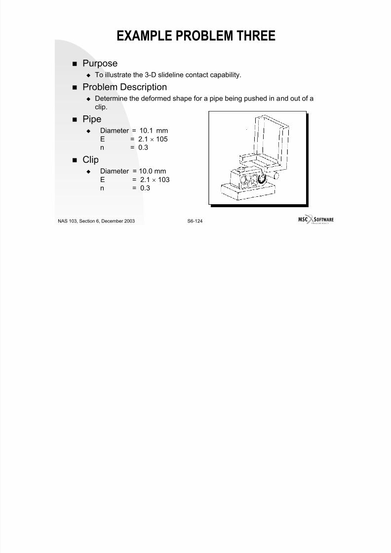
7/21/2019 Nonlinear Analysis Using MSC.nastran
http://slidepdf.com/reader/full/nonlinear-analysis-using-mscnastran 420/783
S6-123NAS 103, Section 6, December 2003
EXAMPLE PROBLEM TWO
Deformed Shapes for the Wedge Model.Deformed Shapes for the AxisymmetricModel.
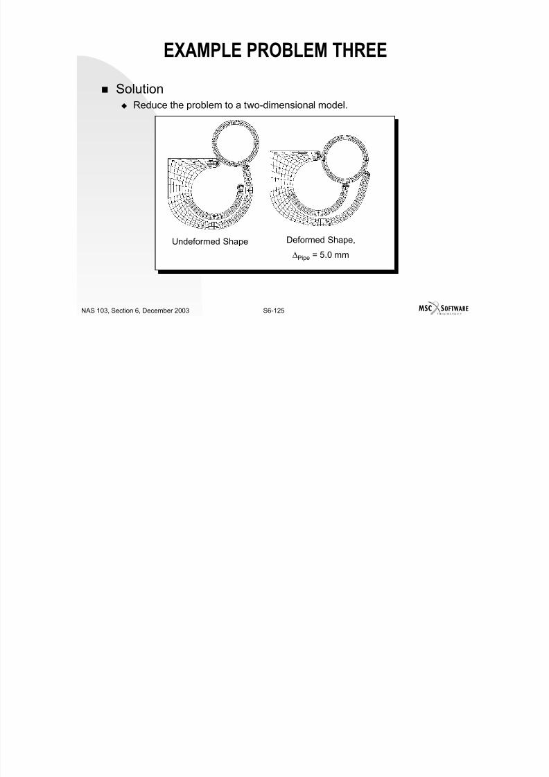
7/21/2019 Nonlinear Analysis Using MSC.nastran
http://slidepdf.com/reader/full/nonlinear-analysis-using-mscnastran 421/783
S6-124NAS 103, Section 6, December 2003
EXAMPLE PROBLEM THREE
Purpose To illustrate the 3-D slideline contact capability.
Problem Description Determine the deformed shape for a pipe being pushed in and out of a
clip.
Pipe Diameter = 10.1 mm
E = 2.1 × 10⁵n = 0.3
Clip Diameter = 10.0 mm
E = 2.1 × 10³n = 0.3

7/21/2019 Nonlinear Analysis Using MSC.nastran
http://slidepdf.com/reader/full/nonlinear-analysis-using-mscnastran 422/783
S6-125NAS 103, Section 6, December 2003
EXAMPLE PROBLEM THREE
Solution Reduce the problem to a two-dimensional model.
Undeformed Shape Deformed Shape,∆Pipe = 5.0 mm

7/21/2019 Nonlinear Analysis Using MSC.nastran
http://slidepdf.com/reader/full/nonlinear-analysis-using-mscnastran 423/783
S6-126NAS 103, Section 6, December 2003
EXAMPLE PROBLEM THREE
Deformed Shape, Deformed Shape
∆Pipe = 10.30 mm ∆Pipe = 7.5 mm
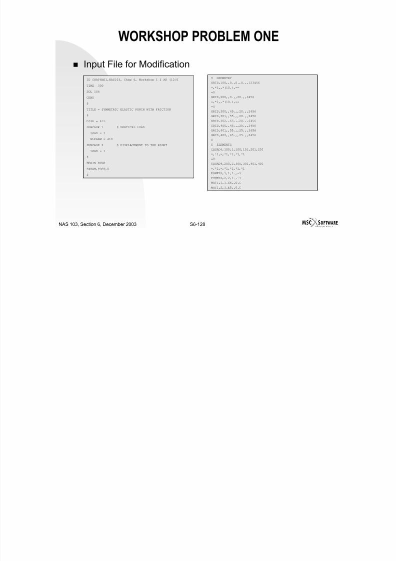
7/21/2019 Nonlinear Analysis Using MSC.nastran
http://slidepdf.com/reader/full/nonlinear-analysis-using-mscnastran 424/783
S6-127NAS 103, Section 6, December 2003
WORKSHOP PROBLEM ONE
Purpose To demonstrate the use of 3-D slideline contact.
Problem Description An elastic punch is punched into an elastic foundation and then movedhorizontally to the right by 30 inches. The details of the model are asshown below.
Modify the input file to define a symmetric contact region. Use the displacement increment to push the punch horizontally to the
right by a total of 10 inches. Use increment of one inch per load step. Plot the deformed shapes at the end of subcases one and two.

7/21/2019 Nonlinear Analysis Using MSC.nastran
http://slidepdf.com/reader/full/nonlinear-analysis-using-mscnastran 425/783
S6-128NAS 103, Section 6, December 2003
WORKSHOP PROBLEM ONE
Input File for Modification
ID CHAP6WS1,NAS103, Chap 6, Workshop 1 $ AR (12/0
TIME 300
SOL 106
CEND
$
TITLE = SYMMETRIC ELASTIC PUNCH WITH FRICTION
$
DISP = ALL
SUBCASE 1 $ VERTICAL LOAD
LOAD = 1
NLPARM = 410
SUBCASE 2 $ DISPLACEMENT TO THE RIGHT
LOAD = 1
$
BEGIN BULK
PARAM,POST,0
$
$ GEOMETRY
GRID,100,,0.,0.,0.,,123456
=,*1,,*(10.),===9
GRID,200,,0.,,20.,,2456
=,*1,,*(10.),==
=9
GRID,300,,45.,,20.,,2456
GRID,301,,55.,,20.,,2456
GRID,302,,65.,,20.,,2456
GRID,400,,45.,,25.,,2456
GRID,401,,55.,,25.,,2456GRID,402,,65.,,25.,,2456
$
$ ELEMENTS
CQUAD4,100,1,100,101,201,200
=,*1,=,*1,*1,*1,*1
=8
CQUAD4,200,2,300,301,401,400
=,*1,=,*1,*1,*1,*1
PSHELL,1,1,1.,-1PSHELL,2,2,1.,-1
MAT1,1,1.E5,,0.0
MAT1,2,1.E5,,0.0
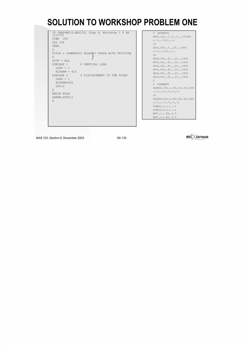
7/21/2019 Nonlinear Analysis Using MSC.nastran
http://slidepdf.com/reader/full/nonlinear-analysis-using-mscnastran 426/783
S6-129NAS 103, Section 6, December 2003
WORKSHOP PROBLEM ONE
$
$ PUNCH LOAD: VERTICAL LOAD
FORCE,1,400,,-1000.,0.,0.,1.
FORCE,1,401,,-2000.,0.,0.,1.
FORCE,1,402,,-1000.,0.,0.,1.
$
$ LOAD FOR SUBCASE 2 : RIGHT HORIZONTAL DISPLACEMENT
$$ SLIDELINE CONTACT
$
$ NONLINEAR SOLUTION STRATEGY: AUTO METHOD WITH DEFAULTS
NLPARM, 410, 1 , ,AUTO, , ,PW, YES, +NLP41
+NLP41, ,1.E-6, 1.E-10
$
ENDDATA
Input File for Modification (Cont’d)
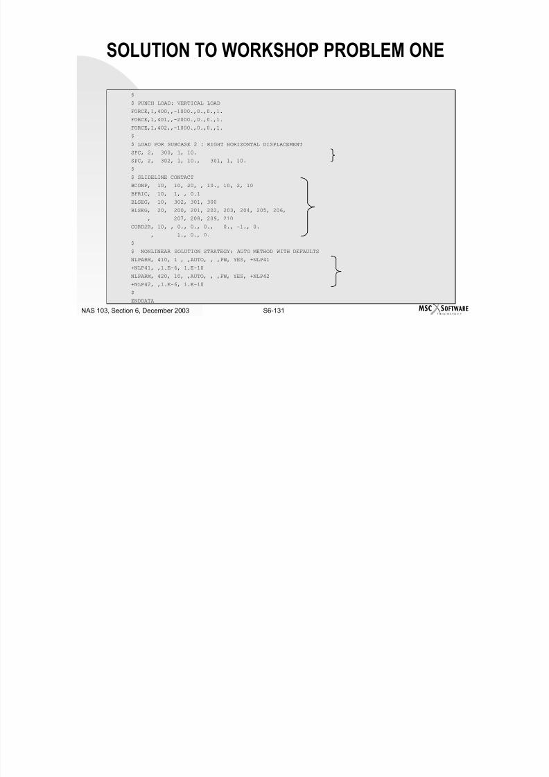
7/21/2019 Nonlinear Analysis Using MSC.nastran
http://slidepdf.com/reader/full/nonlinear-analysis-using-mscnastran 427/783
S6-130NAS 103, Section 6, December 2003
SOLUTION TO WORKSHOP PROBLEM ONEID CHAP6WS1S,NAS103, Chap 6, Workshop 1 $ AR(12/03)
TIME 300
SOL 106
CEND
$
TITLE = SYMMETRIC ELASTIC PUNCH WITH FRICTION$
DISP = ALL
SUBCASE 1 $ VERTICAL LOAD
LOAD = 1
NLPARM = 410
SUBCASE 2 $ DISPLACEMENT TO THE RIGHT
LOAD = 1
NLPARM=420
SPC=2
$
BEGIN BULK
PARAM,POST,0
$
$ GEOMETRY
GRID,100,,0.,0.,0.,,123456
=,*1,,*(10.),==
=9
GRID,200,,0.,,20.,,2456
=,*1,,*(10.),==
=9
GRID,300,,45.,,20.,,2456
GRID,301,,55.,,20.,,2456
GRID,302,,65.,,20.,,2456
GRID,400,,45.,,25.,,2456
GRID,401,,55.,,25.,,2456
GRID,402,,65.,,25.,,2456
$$ ELEMENTS
CQUAD4,100,1,100,101,201,200
=,*1,=,*1,*1,*1,*1
=8
CQUAD4,200,2,300,301,401,400
=,*1,=,*1,*1,*1,*1
PSHELL,1,1,1.,-1PSHELL,2,2,1.,-1
MAT1,1,1.E5,,0.0
MAT1,2,1.E5,,0.0
7/21/2019 Nonlinear Analysis Using MSC.nastran
http://slidepdf.com/reader/full/nonlinear-analysis-using-mscnastran 428/783
S6-131NAS 103, Section 6, December 2003
SOLUTION TO WORKSHOP PROBLEM ONE
$
$ PUNCH LOAD: VERTICAL LOAD
FORCE,1,400,,-1000.,0.,0.,1.
FORCE,1,401,,-2000.,0.,0.,1.FORCE,1,402,,-1000.,0.,0.,1.
$
$ LOAD FOR SUBCASE 2 : RIGHT HORIZONTAL DISPLACEMENT
SPC, 2, 300, 1, 10.
SPC, 2, 302, 1, 10., 301, 1, 10.
$
$ SLIDELINE CONTACT
BCONP, 10, 10, 20, , 10., 10, 2, 10
BFRIC, 10, 1, , 0.1
BLSEG, 10, 302, 301, 300
BLSEG, 20, 200, 201, 202, 203, 204, 205, 206,
, 207, 208, 209, 210
CORD2R, 10, , 0., 0., 0., 0., -1., 0.
, 1., 0., 0.
$
$ NONLINEAR SOLUTION STRATEGY: AUTO METHOD WITH DEFAULTS
NLPARM, 410, 1 , ,AUTO, , ,PW, YES, +NLP41
+NLP41, ,1.E-6, 1.E-10
NLPARM, 420, 10, ,AUTO, , ,PW, YES, +NLP42
+NLP42, ,1.E-6, 1.E-10
$
ENDDATA

7/21/2019 Nonlinear Analysis Using MSC.nastran
http://slidepdf.com/reader/full/nonlinear-analysis-using-mscnastran 429/783
S6-132NAS 103, Section 6, December 2003
SOLUTION TO WORKSHOP PROBLEM ONE

7/21/2019 Nonlinear Analysis Using MSC.nastran
http://slidepdf.com/reader/full/nonlinear-analysis-using-mscnastran 430/783
S7-1NAS 103, Section 7, December, 2003
SECTION 7
NONLINEAR TRANSIENT ANALYSIS
7/21/2019 Nonlinear Analysis Using MSC.nastran
http://slidepdf.com/reader/full/nonlinear-analysis-using-mscnastran 431/783
S7-2NAS 103, Section 7, December, 2003
7/21/2019 Nonlinear Analysis Using MSC.nastran
http://slidepdf.com/reader/full/nonlinear-analysis-using-mscnastran 432/783
S7-3NAS 103, Section 7, December, 2003
TABLE OF CONTENTS
Page
Review Of Transient Analysis 7-5
User Interface 7-11
Example Input For Sol 129 7-15
General Features 7-16
General Limitations 7-17
Integration Schemes 7-18
Nonlinear Transient Solution Strategy 7-21
Mass Specification 7-30
Damping 7-31
Damping Specification 7-34
Load Specification 7-37Dynamic Loads 7-38
Dynamic Loads Example 7-47
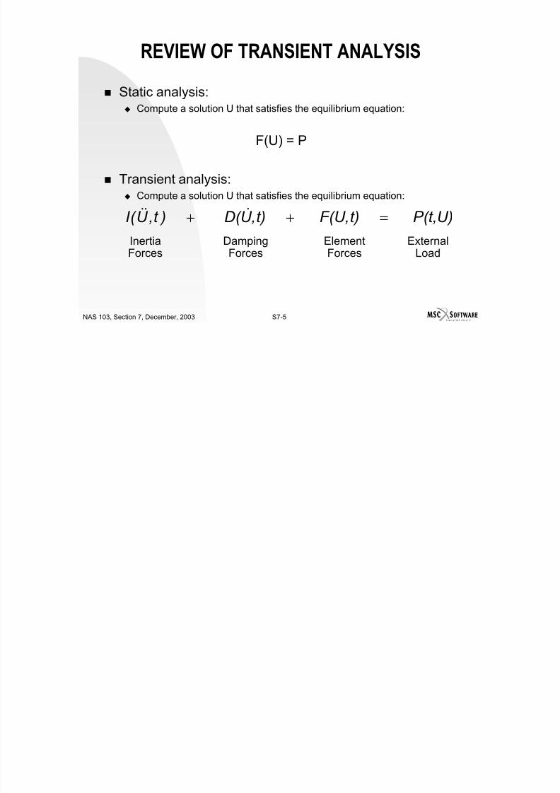
7/21/2019 Nonlinear Analysis Using MSC.nastran
http://slidepdf.com/reader/full/nonlinear-analysis-using-mscnastran 433/783
S7-4NAS 103, Section 7, December, 2003
TABLE OF CONTENTS
PageStatic Loads In Transient Analysis 7-49LSEQ Entry 7-50
Example: Static Loads In Transient Analysis 7-53Nonlinear Loads 7-55Example: Nonlinear Loads 7-63Initial Conditions 7-66
Restarts For Nonlinear Transient Analysis 7-67Hints And Recommendations For Sol 129 7-68Example Problem One 7-69Example Problem Two 7-74Workshop Problems One Through Three 7-76
Workshop Problem Four 7-80Solution For Workshop Problem One 7-84Solution For Workshop Problem Two 7-89Solution For Workshop Problem Three 7-90
Solution To Workshop Problem Four 7-91

7/21/2019 Nonlinear Analysis Using MSC.nastran
http://slidepdf.com/reader/full/nonlinear-analysis-using-mscnastran 434/783
S7-5NAS 103, Section 7, December, 2003
REVIEW OF TRANSIENT ANALYSIS
Static analysis: Compute a solution U that satisfies the equilibrium equation:
F(U) = P
Transient analysis: Compute a solution U that satisfies the equilibrium equation:
U)P(t, t)F(U, t),U D( )t ,U ( I =++ &&&
InertiaForces DampingForces ElementForces ExternalLoad
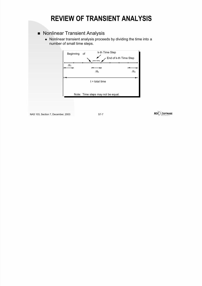
7/21/2019 Nonlinear Analysis Using MSC.nastran
http://slidepdf.com/reader/full/nonlinear-analysis-using-mscnastran 435/783
S7-6NAS 103, Section 7, December, 2003
REVIEW OF TRANSIENT ANALYSIS
For a linear system
For a general nonlinear system Mass of the system may change
Damping may change
Stiffness may change
Load may be function of system response In MSC.NASTRAN mass and damping cannot change. Therefore, the
equilibrium equation is
P(t)KU U BU M =++ &&&
U)P(t,F(U(t))t U B )t ( U M =++ &&&
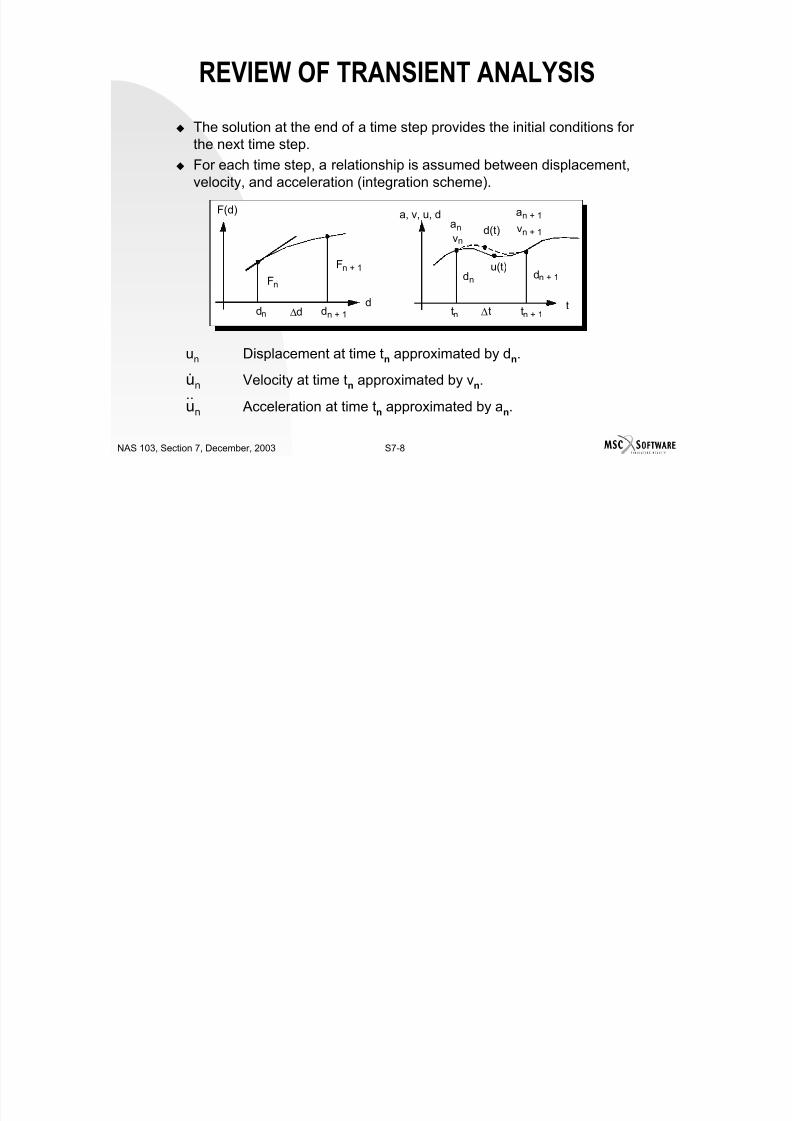
7/21/2019 Nonlinear Analysis Using MSC.nastran
http://slidepdf.com/reader/full/nonlinear-analysis-using-mscnastran 436/783
S7-7NAS 103, Section 7, December, 2003
REVIEW OF TRANSIENT ANALYSIS
Nonlinear Transient Analysis Nonlinear transient analysis proceeds by dividing the time into a
number of small time steps.
Beginning of k-th Time Step
t = total time
End of k-th Time Step
Note: Time steps may not be equal.
∆t1
∆tk ∆tn
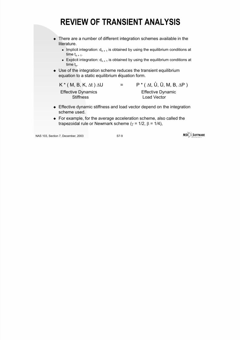
7/21/2019 Nonlinear Analysis Using MSC.nastran
http://slidepdf.com/reader/full/nonlinear-analysis-using-mscnastran 437/783
S7-8NAS 103, Section 7, December, 2003
REVIEW OF TRANSIENT ANALYSIS
The solution at the end of a time step provides the initial conditions forthe next time step.
For each time step, a relationship is assumed between displacement,
velocity, and acceleration (integration scheme).
un Displacement at time tn approximated by dn.
un Velocity at time tn approximated by vn.
un Acceleration at time tn approximated by an.
.
..
t
F(d)
Fn
dn
Fn + 1
dn + 1d
a, v, u, danvn
dn
d(t)
u(t)
∆ttn tn + 1
dn + 1
an + 1
vn + 1
∆d

7/21/2019 Nonlinear Analysis Using MSC.nastran
http://slidepdf.com/reader/full/nonlinear-analysis-using-mscnastran 438/783
S7-9NAS 103, Section 7, December, 2003
REVIEW OF TRANSIENT ANALYSIS
There are a number of different integration schemes available in theliterature. Implicit integration: dn + 1 is obtained by using the equilibrium conditions at
time tn + 1. Explicit integration: dn + 1 is obtained by using the equilibrium conditions at
time tn.
Use of the integration scheme reduces the transient equilibriumequation to a static equilibrium equation form.
Effective dynamic stiffness and load vector depend on the integrationscheme used.
For example, for the average acceleration scheme, also called thetrapezoidal rule or Newmark scheme (γ = 1/2, β = 1/4),
K * ( M, B, K, ∆t ) ∆U = P * ( ∆t, Ů, Ü, M, B, ∆P )
Effective Dynamics Effective DynamicStiffness Load Vector
.
U
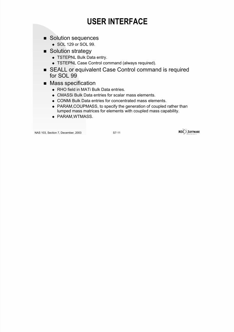
7/21/2019 Nonlinear Analysis Using MSC.nastran
http://slidepdf.com/reader/full/nonlinear-analysis-using-mscnastran 439/783
S7-10NAS 103, Section 7, December, 2003
REVIEW OF TRANSIENT ANALYSIS
The equilibrium is satisfied at the beginning and at the end of a time step. The equilibrium is not satisfied within the time step. Therefore, the selection of ∆t
is important. A large value of ∆t reduces accuracy. A small value of ∆t increases computing cost. A strategy is needed that automatically adjusts the time step value to achieve an
optimum value in terms of accuracy and computing cost. Adjustment of time step value requires the reformation and decomposition of the
dynamic stiffness.
K Bt
M t
K +∆
+∆
=24
2
*
)(2)](4
)(2[)(* t U Bt U t
t U M t P P &&&& +∆
++∆=

7/21/2019 Nonlinear Analysis Using MSC.nastran
http://slidepdf.com/reader/full/nonlinear-analysis-using-mscnastran 440/783
S7-11NAS 103, Section 7, December, 2003
USER INTERFACE
Solution sequences SOL 129 or SOL 99.
Solution strategy TSTEPNL Bulk Data entry. TSTEPNL Case Control command (always required).
SEALL or equivalent Case Control command is required
for SOL 99 Mass specification RHO field in MATi Bulk Data entries. CMASSi Bulk Data entries for scalar mass elements. CONMi Bulk Data entries for concentrated mass elements. PARAM,COUPMASS, to specify the generation of coupled rather than
lumped mass matrices for elements with coupled mass capability. PARAM,WTMASS.

7/21/2019 Nonlinear Analysis Using MSC.nastran
http://slidepdf.com/reader/full/nonlinear-analysis-using-mscnastran 441/783
S7-12NAS 103, Section 7, December, 2003
USER INTERFACE
Damping specification CVISC Bulk Data entry for the viscous damper element.
Field GE in MATi Bulk Data entries for nonlinear element damping PARAM, G for overall structural damping.
PARAM, W3 to convert structural damping to equivalent viscousdamping.
PARAM, W4 to convert element damping to equivalent viscous
damping. PARAM, NDAMP to specify numerical damping.
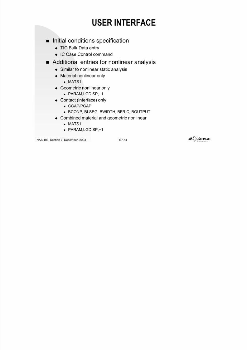
7/21/2019 Nonlinear Analysis Using MSC.nastran
http://slidepdf.com/reader/full/nonlinear-analysis-using-mscnastran 442/783
S7-13NAS 103, Section 7, December, 2003
USER INTERFACE
Load Specification
Selected by DLOAD, LOADSET, and NONLINEAR Case Controlcommands.
Nonlinear transient load as a negative variable raised to a power.NOLIN4Nonlinear transient load as a positive variable raised to a power.NOLIN3
Nonlinear transient load as the product of two variables.NOLIN2
Nonlinear transient load as a tabular function.NOLIN1
Generate transient load history for static loads.LSEQ
Transient load scale factors.DAREATransient load as defined by analytical functions.TLOAD2
Transient load as ordered time, force pairs.TLOAD1
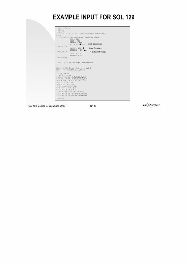
7/21/2019 Nonlinear Analysis Using MSC.nastran
http://slidepdf.com/reader/full/nonlinear-analysis-using-mscnastran 443/783
S7-14NAS 103, Section 7, December, 2003
USER INTERFACE
Initial conditions specification TIC Bulk Data entry
IC Case Control command Additional entries for nonlinear analysis
Similar to nonlinear static analysis
Material nonlinear only
MATS1 Geometric nonlinear only
PARAM,LGDISP,+1
Contact (interface) only CGAP/PGAP
BCONP, BLSEG, BWIDTH, BFRIC, BOUTPUT
Combined material and geometric nonlinear MATS1
PARAM,LGDISP,+1
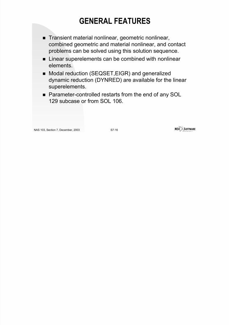
7/21/2019 Nonlinear Analysis Using MSC.nastran
http://slidepdf.com/reader/full/nonlinear-analysis-using-mscnastran 444/783
S7-15NAS 103, Section 7, December, 2003
EXAMPLE INPUT FOR SOL 129
ID MSC, NL129TIME 30SOL 129DIAG 50 $ Print nonlinear iteration informationCENDTITLE = MATERIAL NONLINEAR TRANSIENT ANALYSIS
SPC = 123DISP = ALL
STRESS = ALLIC = 50
SUBCASE 10DLOAD = 100TSTEPNL = 10
SUBCASE 20DLOAD = 200TSTEPNL = 20
BEGIN BULK..
(Usual entries for model definition)..MAT1,10,30.+6,,.3, 0.1, , , 1.E-4MATS1,10,,PLASTIC,0.,,,30.+3$PARAM,LGDISP,1$ LOAD ENTRIESTLOAD2,100,10,,0,0.0,10.0,1.0TLOAD2,110,20,,0,10.0,20.0,1.0DLOAD,200,1.0,1.0,100,1.0,110
DAREA,10,15,1,10.0DAREA,20,18,1,5.0$ INITIAL CONDITIONSTIC,50,5,1,1.0,-2.0TIC,50,6,2,-2.0,4.0$ SOLUTION STRATEGY ENTRIESTSTEPNL,10,10,.01,1,AUTO,,10,PTSTEPNL,20,20,.01,1,AUTO,,10,P$ENDDATA
Initial Conditions
Load Selection
Solution Strategy

7/21/2019 Nonlinear Analysis Using MSC.nastran
http://slidepdf.com/reader/full/nonlinear-analysis-using-mscnastran 445/783
S7-16NAS 103, Section 7, December, 2003
GENERAL FEATURES
Transient material nonlinear, geometric nonlinear,combined geometric and material nonlinear, and contact
problems can be solved using this solution sequence. Linear superelements can be combined with nonlinear
elements.
Modal reduction (SEQSET,EIGR) and generalizeddynamic reduction (DYNRED) are available for the linearsuperelements.
Parameter-controlled restarts from the end of any SOL
129 subcase or from SOL 106.

7/21/2019 Nonlinear Analysis Using MSC.nastran
http://slidepdf.com/reader/full/nonlinear-analysis-using-mscnastran 446/783
S7-17NAS 103, Section 7, December, 2003
GENERAL LIMITATIONS
No constraint changes after first subcase - including restart.
No thermal loads or enforced displacements.
Reduction (GDR, Guyan reduction) only for superelements. PARAM “G” damping only applies to linear elements.
Nonlinear element damping provided by GE on MAT Bulk Dataentries (PARAM “W4” must also be used) only for initial K.
Damping remains constant. No element force output for nonlinear elements.
Upstream loads are ignored in the superelement data recovery.
No grid point stresses for nonlinear elements.
Mass cannot change.

7/21/2019 Nonlinear Analysis Using MSC.nastran
http://slidepdf.com/reader/full/nonlinear-analysis-using-mscnastran 447/783
S7-18NAS 103, Section 7, December, 2003
INTEGRATION SCHEMES
Two-Point Integration Scheme Use the following equilibrium equation:
Assume that the acceleration for a time step is equal to the average ofthe beginning and end of the step.
Velocity and displacement are obtained by integration.
111n1n UU ++++ =++ nn P F B M &&&
2(t)U 1++= nn U U
&&&&
&&
211
11
4
2
t U U
t U U U
t U U
U U
nnnnn
nnnn
∆
++∆+=
∆
++=
++
++
&&&&&
&&&&
&&
INTEGRATION SCHEMES

7/21/2019 Nonlinear Analysis Using MSC.nastran
http://slidepdf.com/reader/full/nonlinear-analysis-using-mscnastran 448/783
S7-19NAS 103, Section 7, December, 2003
INTEGRATION SCHEMES
Rearrange the equilibrium equation in terms of incremental values.
Calculate velocity as follows:
Note that the acceleration need not be calculated since it does notappear in the incremental equilibrium equation.
For postprocessing purposes, acceleration is calculated as:
][24
424
1212 nnnnnnT U U C t
M t
U M t
F P P U K Bt
M t
−
∆
+∆
−∆
+−+=∆
+∆
+∆ ++
&
Dynamic Stiffness Dynamic Load Factor
nnnn U t U U U &&
−∆−= ++
2
)( 11
∆∆
−
∆∆
−∆
∆+
∆∆
∆+∆= −
+
+
+−
++
1
11
1
11
11
n
n
nn
n
n
n
nn
n
n
nn
n U t
t U
t
t
t
t U
t
t
T t U &&&&&&&
INTEGRATION SCHEMES
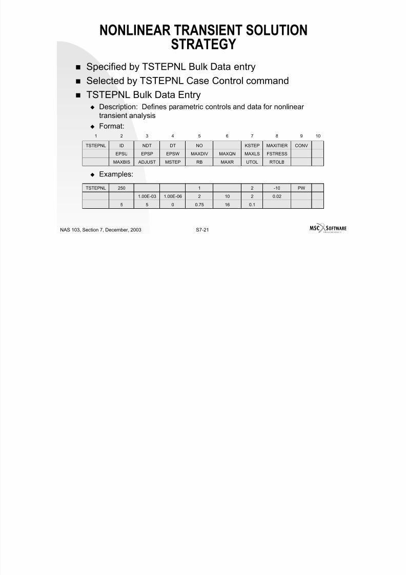
7/21/2019 Nonlinear Analysis Using MSC.nastran
http://slidepdf.com/reader/full/nonlinear-analysis-using-mscnastran 449/783
S7-20NAS 103, Section 7, December, 2003
INTEGRATION SCHEMES
Two-point integration scheme is the same as thetrapezoidal rule or average acceleration method except
for the calculation of acceleration in postprocessing. For linear problems, this scheme is second-order
accurate, is unconditionally stable, and has no numericaldamping.
Easy starting, restarting, ending. Residual error carried over effectively.
Equilibrium is satisfied without the need of calculating 0 U &&
NONLINEAR TRANSIENT SOLUTION

7/21/2019 Nonlinear Analysis Using MSC.nastran
http://slidepdf.com/reader/full/nonlinear-analysis-using-mscnastran 450/783
S7-21NAS 103, Section 7, December, 2003
NONLINEAR TRANSIENT SOLUTION
STRATEGY Specified by TSTEPNL Bulk Data entry
Selected by TSTEPNL Case Control command
TSTEPNL Bulk Data Entry Description: Defines parametric controls and data for nonlinear
transient analysis
Format:
Examples:
RTOLBUTOLMAXRRBMSTEP ADJUSTMAXBIS
FSTRESSMAXLSMAXQNMAXDIVEPSWEPSPEPSU
CONVMAXITIERKSTEPNODTNDTIDTSTEPNL
10987654321
0.1160.75055
0.0221021.00E-061.00E-03
PW-1021250TSTEPNL
NONLINEAR TRANSIENT SOLUTION

7/21/2019 Nonlinear Analysis Using MSC.nastran
http://slidepdf.com/reader/full/nonlinear-analysis-using-mscnastran 451/783
S7-22NAS 103, Section 7, December, 2003
NONLINEAR TRANSIENT SOLUTION
STRATEGYField Contents
ID Identification number. (Integer > 0).
NDT Number of time steps of value DT. (Integer > 4).
DT Time increment. (Real > 0.0).
NO Time step interval for output. Every NO-th step will be savedfor output. (Integer > 0; Default = 1).
KSTEP If METHOD = “TSTEP”, then KSTEP is the time step interval
for stiffness Updates. If METHOD = “ADAPT”, then KSTEPis the number of converged bisection solutions betweenstiffness updates. (Integer > 0; Default = 2)
MAXITER Limit on number of iterations for each time step. (Integer ≠ 0;Default = 10)
NONLINEAR TRANSIENT SOLUTION

7/21/2019 Nonlinear Analysis Using MSC.nastran
http://slidepdf.com/reader/full/nonlinear-analysis-using-mscnastran 452/783
S7-23NAS 103, Section 7, December, 2003
NONLINEAR TRANSIENT SOLUTION
STRATEGYField Contents (Cont.)
CONV Flags to select convergence criteria. (Character: “U”, “P”,“W”, or any combination; Default = “PW”)
EPSU Error tolerance for displacement (U) criterion. (Real > 0.0;Default = 1 .0E-2)
EPSP Error tolerance for load (P) criterion. (Real > 0.0; Default =1.0E-3)
EPSW Error tolerance for work (W) criterion. (Real > 0.0;Default = 1 .0E-6)
MAXDIV Limit on the number of diverging conditions for a time stepbefore the solution is assumed to diverge. (Integer > 0;Default = 2)
MAXQN Maximum number of quasi-Newton correction vectors to besaved on the database. (Integer ≥ 0; Default = 10)
MAXLS Maximum number of line searches allowed per iteration.(Integer ≥ 0; Default = 2)
NONLINEAR TRANSIENT SOLUTION

7/21/2019 Nonlinear Analysis Using MSC.nastran
http://slidepdf.com/reader/full/nonlinear-analysis-using-mscnastran 453/783
S7-24NAS 103, Section 7, December, 2003
O S SO U O
STRATEGYField Contents (Cont.)
FSTRESS Fraction of effective stress (s) used to limit the subincrementsize in the material routines. (0.0 < Real < 1.0;
Default = 0.2)MAXBIS Maximum number of bisections allowed for each time step.
(- 9 ≤ Integer ≤ 9; Default = 5)
ADJUST Time step skip factor for automatic time step adjustment.(Integer ≥ 0; Default = 5)
MSTEP Number of steps to obtain the dominant period response.(10 ≤ Integer ≤ 200; Default = variable between 20 and 40)
RB Define bounds for maintaining the same time step for thestepping function if METHOD = “ADAPT”. (0.1 ≤ Real ≤ 1.0;
Default = 0.75)MAXR Maximum ratio for the adjusted incremental time relative to
DT allowed for time step adjustment. (1.0 ≤ Real ≤ 32.0;Default = 16.0)
NONLINEAR TRANSIENT SOLUTION

7/21/2019 Nonlinear Analysis Using MSC.nastran
http://slidepdf.com/reader/full/nonlinear-analysis-using-mscnastran 454/783
S7-25NAS 103, Section 7, December, 2003
STRATEGYField Contents (Cont.)
UTOL Tolerance on displacement increment beneath which there isno time step adjustment. (0.001 > Real ≤ 1.0; Default = 0.1)
RTOLB Maximum value of incremental rotation (in degrees) allowedper iteration to activate bisection. (Real > 2.0;Default = 20.0)
NONLINEAR TRANSIENT SOLUTION

7/21/2019 Nonlinear Analysis Using MSC.nastran
http://slidepdf.com/reader/full/nonlinear-analysis-using-mscnastran 455/783
S7-26NAS 103, Section 7, December, 2003
STRATEGY Automatic Time Step Adjustment (Adaptive Method)
Two-Point Integration Scheme
Time step is automatically adjusted (Use ADJUST = 0, to deactivate)
Stiffness is automatically updated to improve convergence
(KSTEP = # of converged bisection solutions between stiffness updates)
Accurate, efficient, and user-friendly
Based on the dominant frequency in the incremental deformationpattern:
Number of steps (MSTEP) for a period is adaptive, based on thestiffness ratio:
n
T
n
nn
T
n
n
T
n
n
T
nn
U M U
F F U
U M U
U K U
∆∆−∆
=∆∆∆∆
= − )( 12ω
nnn
n
t MSTEP t
t r
∆=
∆∆
= + 1211
ω
π
NONLINEAR TRANSIENT SOLUTION
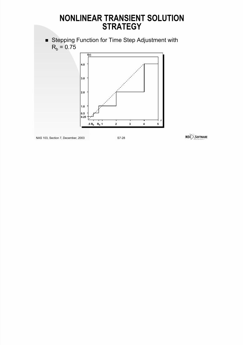
7/21/2019 Nonlinear Analysis Using MSC.nastran
http://slidepdf.com/reader/full/nonlinear-analysis-using-mscnastran 456/783
S7-27NAS 103, Section 7, December, 2003
STRATEGY Thrashing is prevented by the stepping function:
With f = 0.25for r < 0.5 * RBf = 0.5 for 0.5 < RB ≤ r < RBf = 1.0 for RB ≤ r < 2.0
f = 2.0 for 2.0 ≤ r < 3.0/RBf = 4.0 for r ≥ 3.0/RB
Bounds for ∆t adjustment:
Undesirable effects due to GAP, plasticity, large mass, massless points,etc., are filtered out.
nn t r f t ∆=∆ + )(1
MAXR DT t AXR DT n *<∆<
NONLINEAR TRANSIENT SOLUTION

7/21/2019 Nonlinear Analysis Using MSC.nastran
http://slidepdf.com/reader/full/nonlinear-analysis-using-mscnastran 457/783
S7-28NAS 103, Section 7, December, 2003
STRATEGY Stepping Function for Time Step Adjustment with
Rb = 0.75f(r)
4.0
3.0
2.0
1.0
.5 Rb 1 2 3 4 5Rb
0.5
0.25r
NONLINEAR TRANSIENT SOLUTION

7/21/2019 Nonlinear Analysis Using MSC.nastran
http://slidepdf.com/reader/full/nonlinear-analysis-using-mscnastran 458/783
S7-29NAS 103, Section 7, December, 2003
STRATEGY Bisection Algorithm
To overcome divergent problems due to nonlinearity.
Activated when divergence occurs.
Activated when MAXITER is reached.
Activated when excessive ∆σ is detected.
Decomposition at every bisection.
Update [K] at every KSTEP-th converged bisection.
Bisection continues until solution converges or MAXBIS is reached.
If MAXBIS is reached, the reiteration procedure is activated to select thebest attainable solution.
MASS SPECIFICATION
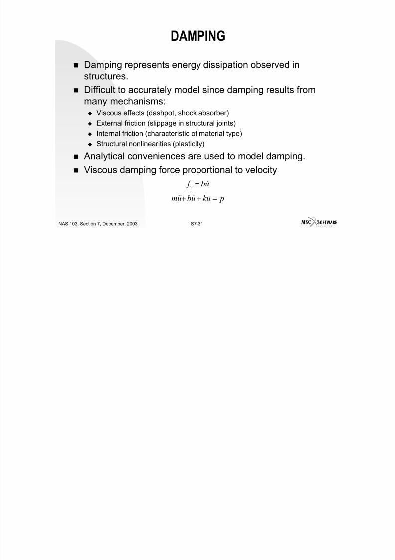
7/21/2019 Nonlinear Analysis Using MSC.nastran
http://slidepdf.com/reader/full/nonlinear-analysis-using-mscnastran 459/783
S7-30NAS 103, Section 7, December, 2003
MASS SPECIFICATION
Similar to linear transient analysis.
CMASS1 and CMASS2 define scalar mass elements.
CMASS3 and CMASS4 define scalar mass elements connectedonly to scalar points.
CONM1 defines a 6 x 6 mass matrix for a grid point.
CONM2 defines a diagonal mass matrix for translational degrees offreedom and a 3 x 3 full matrix for rotational degrees of freedom at agrid point.
Element mass density is defined on the RHO field of the MATi BulkData entry.
PARAM,COUPMASS,1 specifies the coupled mass matrix forelements with coupled mass capability (BAR, BEAM, ROD, HEXA,PENTA, TRIA, and TUBE elements).
DAMPING
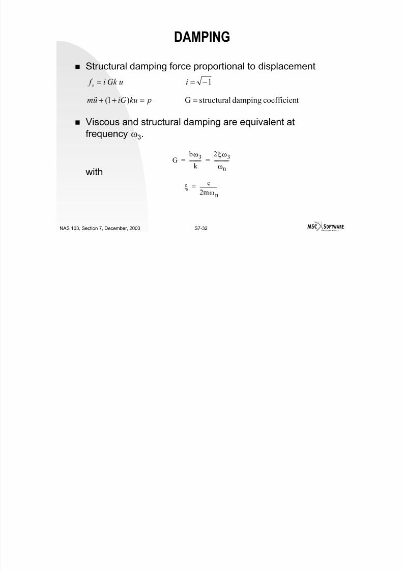
7/21/2019 Nonlinear Analysis Using MSC.nastran
http://slidepdf.com/reader/full/nonlinear-analysis-using-mscnastran 460/783
S7-31NAS 103, Section 7, December, 2003
DAMPING
Damping represents energy dissipation observed instructures.
Difficult to accurately model since damping results frommany mechanisms: Viscous effects (dashpot, shock absorber)
External friction (slippage in structural joints)
Internal friction (characteristic of material type) Structural nonlinearities (plasticity)
Analytical conveniences are used to model damping.
Viscous damping force proportional to velocity
ub f v &=
pkuubum =++ &&&
DAMPING

7/21/2019 Nonlinear Analysis Using MSC.nastran
http://slidepdf.com/reader/full/nonlinear-analysis-using-mscnastran 461/783
S7-32NAS 103, Section 7, December, 2003
DAMPING
Structural damping force proportional to displacement
Viscous and structural damping are equivalent at
frequency ω3.
with
1 −== iuGk i f s
tcoefficiendampingstructuralG )1( ==++ pkuiGum &&
G bω3
k ----------
2ξω3
ωn
-------------= =
ξ c
2mωn
---------------=
DAMPING

7/21/2019 Nonlinear Analysis Using MSC.nastran
http://slidepdf.com/reader/full/nonlinear-analysis-using-mscnastran 462/783
S7-33NAS 103, Section 7, December, 2003
DAMPING
Damping Structural Damping, f s = iGKu
Equivalent
Viscous b = Gk/ω3
ω3 ω
f v b u·=
DAMPING SPECIFICATION

7/21/2019 Nonlinear Analysis Using MSC.nastran
http://slidepdf.com/reader/full/nonlinear-analysis-using-mscnastran 463/783
S7-34NAS 103, Section 7, December, 2003
DAMPING SPECIFICATION
Similar to linear transient analysis.
Damping matrix B comprised of several matrices:
Where B1 = damping elements (VISC,DAMP)
G = overall structural damping coefficient (PARAM,G)
W3 = frequency of interest - rad/sec (PARAM,W3)K1 = global stiffness matrix
Ge = element structural damping coefficient (GE on the MATientry)
W4 = frequency of interest - rad/sec (PARAM,W4
Ke = element stiffness matrix
∑++=e
ee K GW
K W G B B
4
1
3
1 1
DAMPING SPECIFICATION

7/21/2019 Nonlinear Analysis Using MSC.nastran
http://slidepdf.com/reader/full/nonlinear-analysis-using-mscnastran 464/783
S7-35NAS 103, Section 7, December, 2003
G S C C O
Default values for W3 and W4 are 0.0. In this case, the associated dampingterms are ignored.
Nonlinear element damping provided with PARAM,W4 and field GE in the
MATi entry using initial K. Damping matrix is not rotated.
Caution for large rotation.
DAMPING SPECIFICATION

7/21/2019 Nonlinear Analysis Using MSC.nastran
http://slidepdf.com/reader/full/nonlinear-analysis-using-mscnastran 465/783
S7-36NAS 103, Section 7, December, 2003
DAMPING PARAMETERS PARAM,G, factor (default = 0.0)
Overall structural damping coefficient to multiply stiffness matrix for linear
elements. PARAM,W3, factor (default = 0.0)
Converts overall structural damping to equivalent viscous damping.
PARAM,W4 factor (default = 0.0)
Converts element structural damping to equivalent viscous damping. Units for W3,W4 are radians/unit time.
If PARAM,G is used; PARAM,W3 must be set to greater than zero or PARAM,G will be ignored.
LOAD SPECIFICATION

7/21/2019 Nonlinear Analysis Using MSC.nastran
http://slidepdf.com/reader/full/nonlinear-analysis-using-mscnastran 466/783
S7-37NAS 103, Section 7, December, 2003
Three ways: Dynamic loads
Static loads
Nonlinear loads
DYNAMIC LOADS

7/21/2019 Nonlinear Analysis Using MSC.nastran
http://slidepdf.com/reader/full/nonlinear-analysis-using-mscnastran 467/783
S7-38NAS 103, Section 7, December, 2003
Dynamic loads require both temporal and spatialdistribution.
A user needs to follow four steps to specify dynamicloads.
The four steps are:1. Define the load as a function of time (TLOADi).
2. Define the spatial distribution of the load (DAREA).3. Combine the TLOADi entries via DLOAD entry.
4. Select the loads via the DLOAD Case Control command.
DYNAMIC LOADS
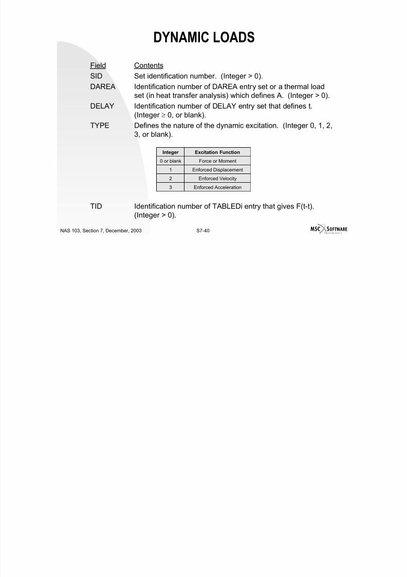
7/21/2019 Nonlinear Analysis Using MSC.nastran
http://slidepdf.com/reader/full/nonlinear-analysis-using-mscnastran 468/783
S7-39NAS 103, Section 7, December, 2003
TLOAD1 Bulk Data Entry Description: Defines a time-dependent dynamic load or enforced
motion of the form
for use in transient response analysis.
Format:
Example:
)t ( F * A )t ( P τ −=
TIDTYPEDELAYDAREASIDTLOAD1
10987654321
1375TLOAD1
DYNAMIC LOADS

7/21/2019 Nonlinear Analysis Using MSC.nastran
http://slidepdf.com/reader/full/nonlinear-analysis-using-mscnastran 469/783
S7-40NAS 103, Section 7, December, 2003
Field Contents
SID Set identification number. (Integer > 0).
DAREA Identification number of DAREA entry set or a thermal load
set (in heat transfer analysis) which defines A. (Integer > 0).DELAY Identification number of DELAY entry set that defines t.
(Integer ≥ 0, or blank).
TYPE Defines the nature of the dynamic excitation. (Integer 0, 1, 2,3, or blank).
TID Identification number of TABLEDi entry that gives F(t-t).(Integer > 0).
Enforced Acceleration3
Enforced Velocity2
Enforced Displacement1
Force or Moment0 or blank
Excitation FunctionInteger
DYNAMIC LOADS

7/21/2019 Nonlinear Analysis Using MSC.nastran
http://slidepdf.com/reader/full/nonlinear-analysis-using-mscnastran 470/783
S7-41NAS 103, Section 7, December, 2003
DAREA Bulk Data Entry Description: Defines scale (area) factors for dynamic loads. DAREA is
used in conjunction with RLOADi and TLOADi entries.
Format:
Example:
Field ContentsSID Identification number. (Integer > 0).Pi Grid, extra, or scalar point identification number.(Integer > 0).Ci Component number. (Integer 1 through 6 for grid point;
blank or 0 for extra or scalar point). Ai Scale (area) factor. (Real).
A2C2P2 A1C1P1SIDDARIA
10987654321
10.11158.2263DARIA
DYNAMIC LOADS

7/21/2019 Nonlinear Analysis Using MSC.nastran
http://slidepdf.com/reader/full/nonlinear-analysis-using-mscnastran 471/783
S7-42NAS 103, Section 7, December, 2003
TLOAD2 Bulk Data Entry Description: Defines a time-dependent dynamic load or enforced
motion of the form
for use in a transient response problem where = t - T1 - t.
Format:
Example:
+≤≤++
+>+<=
)(T2t)(T1, )~
2cos(~
)(T2or t)(T1t, 0)( ~
τ τ π
τ τ
P t F et At P
t C
t ~
BC
PFT2T1TYPEDELAYDAREASIDTLOAD2
10987654321
2
124.72.1104TLOAD2
DYNAMIC LOADS

7/21/2019 Nonlinear Analysis Using MSC.nastran
http://slidepdf.com/reader/full/nonlinear-analysis-using-mscnastran 472/783
S7-43NAS 103, Section 7, December, 2003
Field Contents
SID Set identification number. (Integer > 0).
DAREA Identification number of DAREA entry set or a thermal load
set (in heat transfer analysis) that defines A. (Integer > 0).DELAY Identification number of DELAY entry set that defines t.
(Integer ≥ 0, or blank).
TYPE Defines the nature of the dynamic excitation. (Integer 0, 1, 2,3 or blank).
T1 Time constant. (Real ≥ 0.0).
T2 Time constant. (Real; T2 > T1).
F Frequency in cycles per unit time. (Real ≥ 0.0; Default =0.0).
P Phase angle in degrees. (Real; Default = 0.0).C Exponential coefficient. (Real; Default = 0.0).
B Growth coefficient. (Real; Default = 0.0).
DYNAMIC LOADS

7/21/2019 Nonlinear Analysis Using MSC.nastran
http://slidepdf.com/reader/full/nonlinear-analysis-using-mscnastran 473/783
S7-44NAS 103, Section 7, December, 2003
For a constant load, leave fields F, P, C, and B blank.
For a cosine wave, specify F = 1.0, and leave fields P, C,
and B blank. For a sine wave, specify F = 1.0, P = - 90° and leave
fields C and B blank.
DYNAMIC LOADS

7/21/2019 Nonlinear Analysis Using MSC.nastran
http://slidepdf.com/reader/full/nonlinear-analysis-using-mscnastran 474/783
S7-45NAS 103, Section 7, December, 2003
DLOAD Bulk Data Entry Description: Defines a dynamic loading condition for frequency
response or transient response problems as a linear combination of
load sets defined via RLOAD1 or RLOAD2 entries for frequencyresponse or TLOAD1 or TLOAD2 entries for transient response.
Format:
Example:
L4S4
L3S3L2S2L1S1SSIDDLOAD
10987654321
9-2
827-262117DLOAD
DYNAMIC LOADS
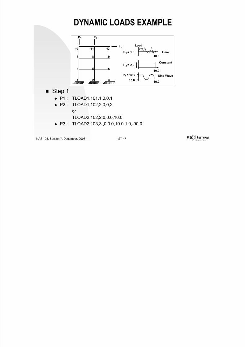
7/21/2019 Nonlinear Analysis Using MSC.nastran
http://slidepdf.com/reader/full/nonlinear-analysis-using-mscnastran 475/783
S7-46NAS 103, Section 7, December, 2003
Field Contents
Sid Load set identification number. (Integer > 0).
S Scale factor. (Real).
Si Scale Factors. (Real).Li Load set identification numbers of RLOAD1, RLOAD2,
TLOAD1, and TLOAD2 entries. (Integer > 0).
DYNAMIC LOADS EXAMPLE

7/21/2019 Nonlinear Analysis Using MSC.nastran
http://slidepdf.com/reader/full/nonlinear-analysis-using-mscnastran 476/783
S7-47NAS 103, Section 7, December, 2003
Step 1 P1 : TLOAD1,101,1,0,0,1
P2 : TLOAD1,102,2,0,0,2
or TLOAD2,102,2,0,0.0,10.0
P3 : TLOAD2,103,3,,0,0.0,10.0,1.0,-90.0
Constant
P1 P3
P210 11 12
7 8 9
4 5 6
1 2 3
10.0
TimeP1 = 1.0
Load
Sine Wave
10.0
10.010.0
P2 = 2.0
P3 = 10.0
DYNAMIC LOADS EXAMPLE

7/21/2019 Nonlinear Analysis Using MSC.nastran
http://slidepdf.com/reader/full/nonlinear-analysis-using-mscnastran 477/783
S7-48NAS 103, Section 7, December, 2003
Step 2 DAREA,1,10,2,-1.0
DAREA,2,12,1,-2.0
DAREA,3,11,2,-10.0
Step 3 DLOAD,10,1.0,1.0,101,1.0,102,1.0,103
Step 4 DLOAD=10 in Case Control
STATIC LOADS IN TRANSIENT ANALYSIS
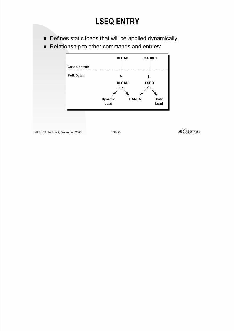
7/21/2019 Nonlinear Analysis Using MSC.nastran
http://slidepdf.com/reader/full/nonlinear-analysis-using-mscnastran 478/783
S7-49NAS 103, Section 7, December, 2003
A user needs to follow five steps to specify static loads intransient analysis.
The five steps are:1. Define the static loads using FORCEi, GRAV, MOMENTi, etc., that arereferenced by the LOAD Case Control command.
2. Define a LSEQ Bulk Data entry to point to a TLOADi entry and to a loadset that is referenced by a LOAD Case Control command.
3. Define a TLOAD1 or TLOAD2 entry to define a constant function withtime.
4. Combine all the TLOADi entries through the DLOAD Bulk Data entry.
5. Select the DLOAD entry through the DLOAD Case Control command
and the LSEQ entry through the LOADSET Case Control command.
LSEQ ENTRY

7/21/2019 Nonlinear Analysis Using MSC.nastran
http://slidepdf.com/reader/full/nonlinear-analysis-using-mscnastran 479/783
S7-50NAS 103, Section 7, December, 2003
Defines static loads that will be applied dynamically.
Relationship to other commands and entries:
DLOAD LOADSET
DLOAD LSEQ
Case Control:
Bulk Data:
Dynamic
Load
DAREA Static
Load
LSEQ ENTRY

7/21/2019 Nonlinear Analysis Using MSC.nastran
http://slidepdf.com/reader/full/nonlinear-analysis-using-mscnastran 480/783
S7-51NAS 103, Section 7, December, 2003
LSEQ Bulk Data Entry Description: Defines a sequence of static load sets.
Format:
Example:
Field Contents
SID Set identification of the set of LSEQ entries. (Integer > 0).
DAREA The DAREA set identification assigned to this static loadvector. (Integer > 0).
TIDLIDDAREASIDLSEQ
10987654321
10011000200100LSEQ
LSEQ ENTRY
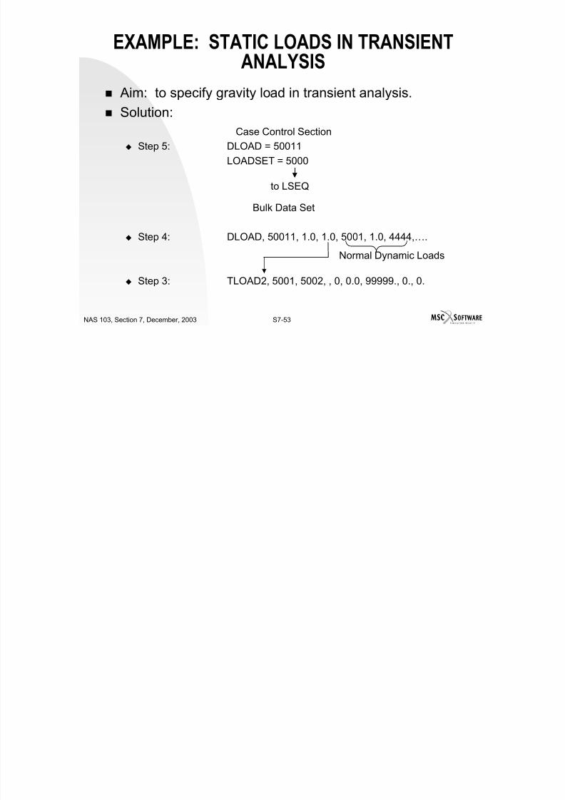
7/21/2019 Nonlinear Analysis Using MSC.nastran
http://slidepdf.com/reader/full/nonlinear-analysis-using-mscnastran 481/783
S7-52NAS 103, Section 7, December, 2003
Field Contents
LID Load set identification number of a set of static load entriessuch as those Referenced by the LOAD Case Control
command. (Integer > 0 or blank).TID Temperature set identification of a set of thermal load entriessuch as those referenced by the TEMP(LOAD) Case Controlcommand. (Integer > 0 or blank).
EXAMPLE: STATIC LOADS IN TRANSIENTANALYSIS

7/21/2019 Nonlinear Analysis Using MSC.nastran
http://slidepdf.com/reader/full/nonlinear-analysis-using-mscnastran 482/783
S7-53NAS 103, Section 7, December, 2003
Aim: to specify gravity load in transient analysis.
Solution:
Case Control Section Step 5: DLOAD = 50011
LOADSET = 5000
Bulk Data Set
Step 4: DLOAD, 50011, 1.0, 1.0, 5001, 1.0, 4444,….
Step 3: TLOAD2, 5001, 5002, , 0, 0.0, 99999., 0., 0.
to LSEQ
Normal Dynamic Loads
EXAMPLE: STATIC LOADS IN TRANSIENTANALYSIS

7/21/2019 Nonlinear Analysis Using MSC.nastran
http://slidepdf.com/reader/full/nonlinear-analysis-using-mscnastran 483/783
S7-54NAS 103, Section 7, December, 2003
Step 3: TLOAD2, 5001, 5002, , 0, 0.0, 99999., 0., 0.
Step 2: LSEQ, 5000, 5002, 5555
Step 1: GRAV, 5555, , 380., 0., 0., 1.0
Defines a function = cos (0) = 1.0
LOADSET DAREA
NONLINEAR LOADS

7/21/2019 Nonlinear Analysis Using MSC.nastran
http://slidepdf.com/reader/full/nonlinear-analysis-using-mscnastran 484/783
S7-55NAS 103, Section 7, December, 2003
Allows for the specification of load at a particular degreeof freedom to be the function of displacement andvelocity at another degree of freedom.
Example:
Load at grid point 1, displacement component 2 as afunction of the displacement component 1 at grid point 3.
P(t)
65 4 3 2 1
P(t) = f (u3)
NONLINEAR LOADS

7/21/2019 Nonlinear Analysis Using MSC.nastran
http://slidepdf.com/reader/full/nonlinear-analysis-using-mscnastran 485/783
S7-56NAS 103, Section 7, December, 2003
Useful for specifying nonlinear springs and nonlineardamping.
Nonlinear loads are specified using NOLINi entries. Four NOLINi entries (NOLIN1, NOLIN2, NOLIN3, and
NOLIN4) to specify mechanical loads.
Nonlinear loads are selected via the NONLINEAR Case
Control command. Nonlinear loads cannot be selected via the DLOAD Case
Control command.
All degrees of freedom referenced on NOLINi entry mustbe members of the solution set.
NONLINEAR LOADS

7/21/2019 Nonlinear Analysis Using MSC.nastran
http://slidepdf.com/reader/full/nonlinear-analysis-using-mscnastran 486/783
S7-57NAS 103, Section 7, December, 2003
Velocity for an independent degree of freedom (for thepurpose of loads) is calculated as
Note: This may be different from that calculated in theintegration scheme. But it is acceptable.
In all NOLINi entries a degree of freedom is specified bythe grid number and its component number.
All loads generated with NOLINi entries lag behind by one
time step ∆t.
t
t t t
t
U U U
∆
∆−−=&
NONLINEAR LOADS
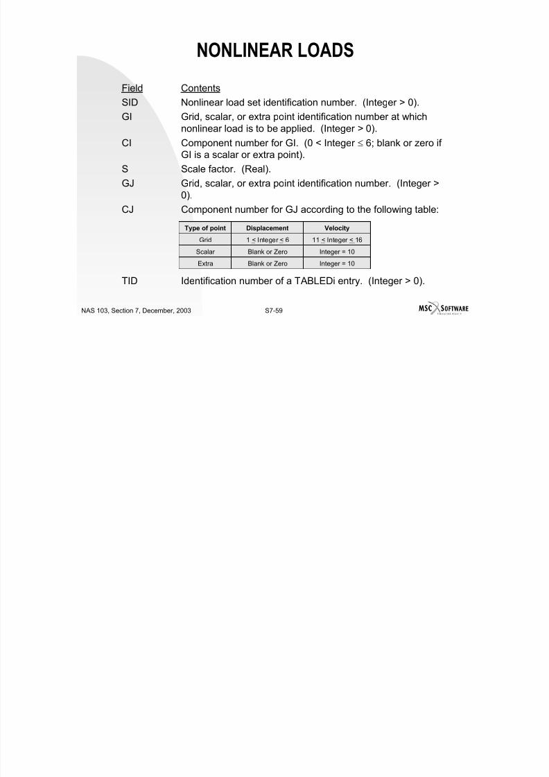
7/21/2019 Nonlinear Analysis Using MSC.nastran
http://slidepdf.com/reader/full/nonlinear-analysis-using-mscnastran 487/783
S7-58NAS 103, Section 7, December, 2003
NOLIN1 Bulk Data Entry Description: Defines nonlinear transient forcing functions of the form.
Function of displacement: Pi(t) = S * T(u j(t)) (1)
Function of velocity: Pi(t) = S * T(u j(t)) (2)where u j(t) and u j(t) are the displacement and velocity at point GJ in thedirection of CJ.
Format:
Example:
.
.
TIDCJGJSC1G1SIDNOLIN1
10987654321
61032.14321NOLIN1
NONLINEAR LOADS

7/21/2019 Nonlinear Analysis Using MSC.nastran
http://slidepdf.com/reader/full/nonlinear-analysis-using-mscnastran 488/783
S7-59NAS 103, Section 7, December, 2003
Field Contents
SID Nonlinear load set identification number. (Integer > 0).
GI Grid, scalar, or extra point identification number at which
nonlinear load is to be applied. (Integer > 0).CI Component number for GI. (0 < Integer ≤ 6; blank or zero if
GI is a scalar or extra point).
S Scale factor. (Real).
GJ Grid, scalar, or extra point identification number. (Integer >0).
CJ Component number for GJ according to the following table:
TID Identification number of a TABLEDi entry. (Integer > 0).
Integer = 10Blank or ZeroExtra
Integer = 10Blank or ZeroScalar
11 < Integer < 161 < Integer < 6Grid
VelocityDisplacementType of point
NONLINEAR LOADS

7/21/2019 Nonlinear Analysis Using MSC.nastran
http://slidepdf.com/reader/full/nonlinear-analysis-using-mscnastran 489/783
S7-60NAS 103, Section 7, December, 2003
NOLIN2 Bulk Data Entry Description: Defines nonlinear transient forcing functions of the form.
where and can be either displacement or velocity at points GJ and GKin the directions of CJ and CK.
Format:
Example:
Pi(t) = S * X j(t) * Xk(t)
CKGKCJGJSC1G1SIDNOLIN2
10987654321
2122.91214NOLIN2
NONLINEAR LOADS

7/21/2019 Nonlinear Analysis Using MSC.nastran
http://slidepdf.com/reader/full/nonlinear-analysis-using-mscnastran 490/783
S7-61NAS 103, Section 7, December, 2003
NOLIN3 Bulk Data Entry Description: Defines nonlinear transient forcing functions of the form.
where may be a displacement or a velocity at point GJ in the directionof CJ.
Format:
Example:
≤
>= 0)(, 0
0)(,)]([*)( t X
t X t X S t P
j
j
A
j
i
ACJGJ5C1G1SIDNOLIN3
10987654321
2152-6.11024NOLIN3
NONLINEAR LOADS
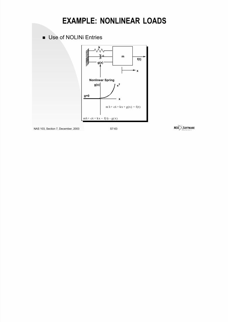
7/21/2019 Nonlinear Analysis Using MSC.nastran
http://slidepdf.com/reader/full/nonlinear-analysis-using-mscnastran 491/783
S7-62NAS 103, Section 7, December, 2003
NOLIN4 Bulk Data Entry Description: Defines nonlinear transient forcing functions of the form.
where may be a displacement or a velocity at point GJ in the directionof CJ.
Format:
Example:
≥<−−= 0)(, 0 0)(,)]([*)(
t X t X t X S t P
j
j
A
ji
ACJGJSC1G1SIDNOLIN4
10987654321
16.31012642NOLIN4
EXAMPLE: NONLINEAR LOADS
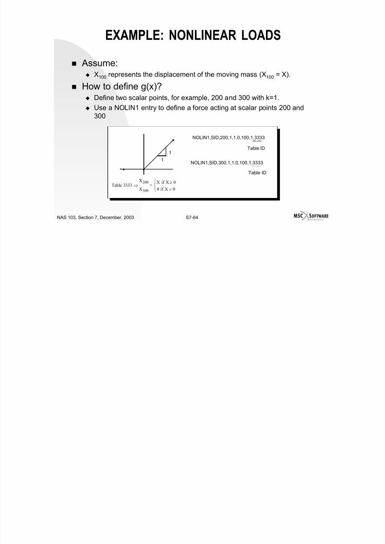
7/21/2019 Nonlinear Analysis Using MSC.nastran
http://slidepdf.com/reader/full/nonlinear-analysis-using-mscnastran 492/783
S7-63NAS 103, Section 7, December, 2003
Use of NOLINi Entries
k
c
g(x)
mf(t)
x
Nonlinear Spring
x
g(x)
g=0
x2
m x·· cx· kx g x( ) f t( )=+ + +
mx·· cx· kx f t( ) g x( ) – =+ +
EXAMPLE: NONLINEAR LOADS

7/21/2019 Nonlinear Analysis Using MSC.nastran
http://slidepdf.com/reader/full/nonlinear-analysis-using-mscnastran 493/783
S7-64NAS 103, Section 7, December, 2003
Assume: X100 represents the displacement of the moving mass (X100 = X).
How to define g(x)? Define two scalar points, for example, 200 and 300 with k=1.
Use a NOLIN1 entry to define a force acting at scalar points 200 and300
1
1
Table 3333X200
X300
X if X 0≥
0 if X 0<
=⇒
NOLIN1,SID,200,1,1.0,100,1,3333
NOLIN1,SID,300,1,1.0,100,1,3333
Table ID
Table ID
EXAMPLE: NONLINEAR LOADS

7/21/2019 Nonlinear Analysis Using MSC.nastran
http://slidepdf.com/reader/full/nonlinear-analysis-using-mscnastran 494/783
S7-65NAS 103, Section 7, December, 2003
Use a NOLIN2 entry to define a force acting at GRID100:
NOLIN2,SID,100,1,-1.000,200,1,300,1
⇒ We define a force acting at the mass (GRID 100) equal
to
Note: This approach is more accurate than using just one NOLIN1 to
define -g(x), where Table 3333 would be a square function rather than alinear function.
≤
>−
0Xif 0
0X2 if X
INITIAL CONDITIONS

7/21/2019 Nonlinear Analysis Using MSC.nastran
http://slidepdf.com/reader/full/nonlinear-analysis-using-mscnastran 495/783
S7-66NAS 103, Section 7, December, 2003
May impose initial displacements and/or velocities with aTIC Bulk Data entry.
IC Case Control command selects TIC entries in theBulk Data Section.
Warning: Initial conditions for unspecified degrees offreedom are set to zero.
Initial conditions may be specified only for A-set degreesof freedom.
RESTARTS FOR NONLINEAR TRANSIENTANALYSIS
St ti f i t i t l i

7/21/2019 Nonlinear Analysis Using MSC.nastran
http://slidepdf.com/reader/full/nonlinear-analysis-using-mscnastran 496/783
S7-67NAS 103, Section 7, December, 2003
Starting from a previous transient analysis Restarts are allowed only from the end of subcases. Set parameters:
PARAM,LOOPID,I I = loop number on printoutPARAM,STIME,To To = starting value of time To should be the last printed value for subcase I. The database will be modified starting from LOOPID+1, T = To.
Starting from a previous nonlinear static analysis Set parameter:PARAM,SLOOPID,I I = loop number on SOL 106 run
Initial transient load should be identical to static loads at restart state.(SPC, etc., may change)
Caution:The database will be completely overwritten.Transient analysis will destroy the static analysisdatabase.
HINTS AND RECOMMENDATIONS FOR SOL129
Id tif th t f li it
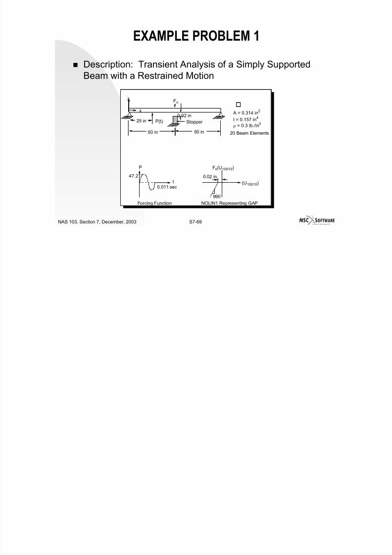
7/21/2019 Nonlinear Analysis Using MSC.nastran
http://slidepdf.com/reader/full/nonlinear-analysis-using-mscnastran 497/783
S7-68NAS 103, Section 7, December, 2003
Identify the type of nonlinearity. Localize nonlinear region. Divide time history by subcases for convenience. Each subcase should not have more than 200 time
steps. Select default values to start - TSTEPNL.
Pick time step size for highest frequency of interest.Twelve or more steps per cycle and frequent content ofinput.
Some damping is desirable for numerical stability.
Avoid massless degrees of freedom. Choose GAP stiffness carefully. Increase MAXITER if convergency is poor.
EXAMPLE PROBLEM 1
D i ti T i t A l i f Si l S t d

7/21/2019 Nonlinear Analysis Using MSC.nastran
http://slidepdf.com/reader/full/nonlinear-analysis-using-mscnastran 498/783
S7-69NAS 103, Section 7, December, 2003
Description: Transient Analysis of a Simply SupportedBeam with a Restrained Motion
0.02 in
990
25 in
50 in
0.02 in
Fnz
x
Stopper P(t)
Fn(U10010)
(U10010)0.011 sec
t
P
47.2
Forcing Function NOLIN1 Representing GAP
20 Beam Elements50 in
A = 0.314 in2
I = 0.157 in4
ρ = 0.3 lb./in3
EXAMPLE PROBLEM 1 (Contd.)
Di l t t th L di P i t (DT 0 0002)
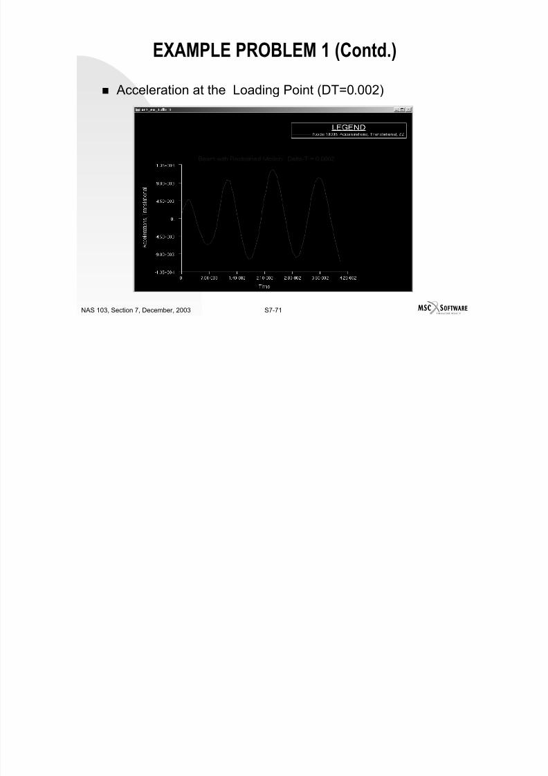
7/21/2019 Nonlinear Analysis Using MSC.nastran
http://slidepdf.com/reader/full/nonlinear-analysis-using-mscnastran 499/783
S7-70NAS 103, Section 7, December, 2003
Displacement at the Loading Point (DT=0.0002)
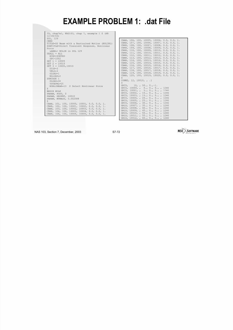
7/21/2019 Nonlinear Analysis Using MSC.nastran
http://slidepdf.com/reader/full/nonlinear-analysis-using-mscnastran 500/783
EXAMPLE PROBLEM 1: .dat File
ID, chap7e1, NAS103, chap 7, example 1 $ (AR12/28/03)
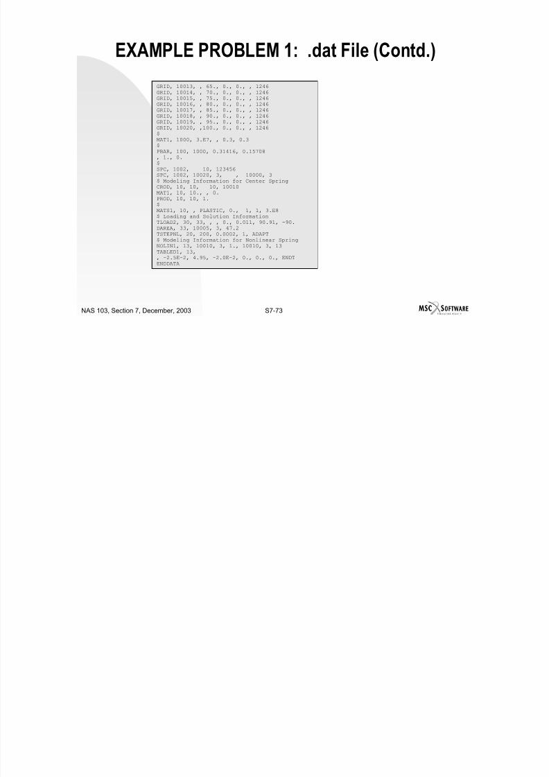
7/21/2019 Nonlinear Analysis Using MSC.nastran
http://slidepdf.com/reader/full/nonlinear-analysis-using-mscnastran 501/783
S7-72NAS 103, Section 7, December, 2003
SOL, 129CENDTITLE=SS Beam with a Restrained Motion (NOLIN1)SUBTITLE=Direct Transient Response, NonlinearForceLABEL= NOLIN in SOL 129
SEALL = ALL
ECHO=SORTEDSPC=1002SET 1 = 10005SET 2 = 10010SET 3 = 10005,10010DISP=3VELO=3OLOAD=1NLLOAD=2
SUBCASE 1
DLOAD=30TSTEPNL=20NONLINEAR=13 $ Select Nonlinear Force
$BEGIN BULKPARAM, POST, 0PARAM, GRDPNT, 10010PARAM, WTMASS, 0.002588$CBAR, 101, 100, 10000, 10001, 0.0, 0.0, 1.
CBAR, 102, 100, 10001, 10002, 0.0, 0.0, 1.CBAR, 103, 100, 10002, 10003, 0.0, 0.0, 1.CBAR, 104, 100, 10003, 10004, 0.0, 0.0, 1.CBAR, 105, 100, 10004, 10005, 0.0, 0.0, 1.
CBAR, 106, 100, 10005, 10006, 0.0, 0.0, 1.CBAR, 107, 100, 10006, 10007, 0.0, 0.0, 1.CBAR, 108, 100, 10007, 10008, 0.0, 0.0, 1.CBAR, 109, 100, 10008, 10009, 0.0, 0.0, 1.CBAR, 110, 100, 10009, 10010, 0.0, 0.0, 1.CBAR, 111, 100, 10010, 10011, 0.0, 0.0, 1.CBAR, 112, 100, 10011, 10012, 0.0, 0.0, 1.CBAR, 113, 100, 10012, 10013, 0.0, 0.0, 1.CBAR, 114, 100, 10013, 10014, 0.0, 0.0, 1.CBAR, 115, 100, 10014, 10015, 0.0, 0.0, 1.CBAR, 116, 100, 10015, 10016, 0.0, 0.0, 1.CBAR, 117, 100, 10016, 10017, 0.0, 0.0, 1.CBAR, 118, 100, 10017, 10018, 0.0, 0.0, 1.CBAR, 119, 100, 10018, 10019, 0.0, 0.0, 1.CBAR, 120, 100, 10019, 10020, 0.0, 0.0, 1.$CONM2, 12, 10010, , .1$GRID, 10, , 50., 0.,-1.GRID, 10000, , 0., 0., 0., , 1246GRID, 10001, , 5., 0., 0., , 1246GRID, 10002, , 10., 0., 0., , 1246GRID, 10003, , 15., 0., 0., , 1246GRID, 10004, , 20., 0., 0., , 1246GRID, 10005, , 25., 0., 0., , 1246GRID, 10006, , 30., 0., 0., , 1246GRID, 10007, , 35., 0., 0., , 1246GRID, 10008, , 40., 0., 0., , 1246GRID, 10009, , 45., 0., 0., , 1246GRID, 10010, , 50., 0., 0., , 1246GRID, 10011, , 55., 0., 0., , 1246GRID, 10012, , 60., 0., 0., , 1246
EXAMPLE PROBLEM 1: .dat File (Contd.)
GRID, 10013, , 65., 0., 0., , 1246
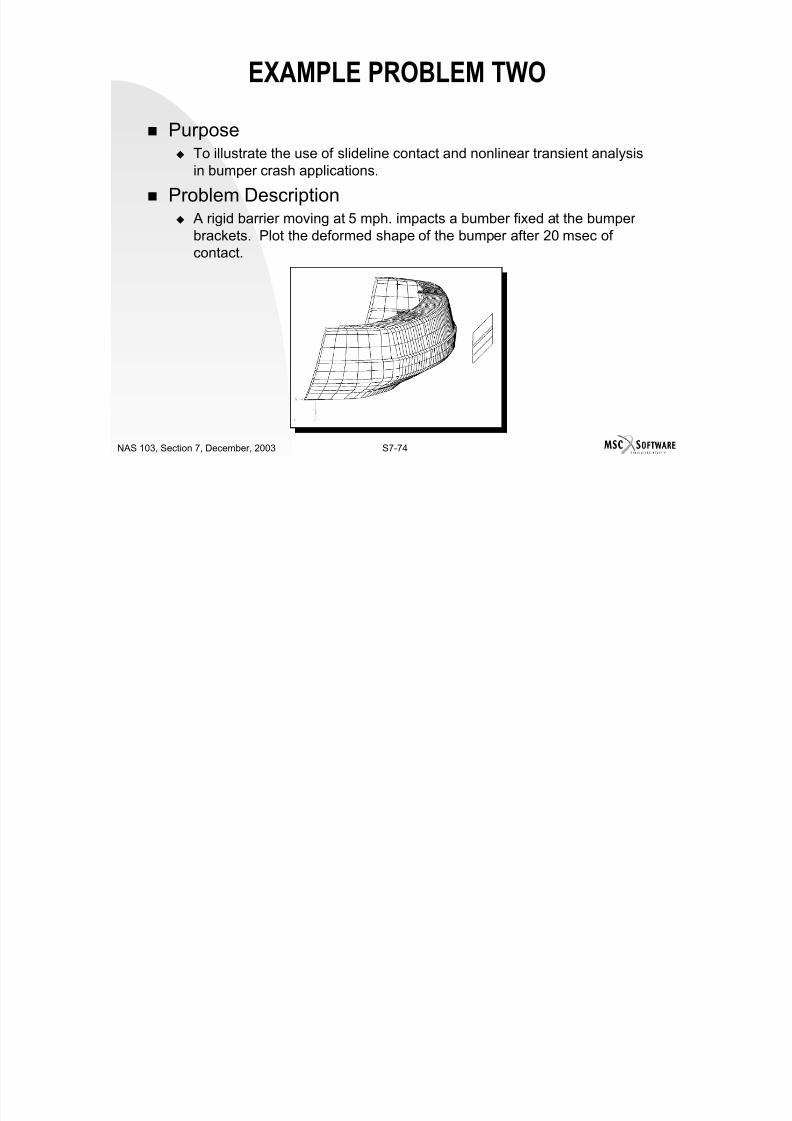
7/21/2019 Nonlinear Analysis Using MSC.nastran
http://slidepdf.com/reader/full/nonlinear-analysis-using-mscnastran 502/783
S7-73NAS 103, Section 7, December, 2003
GRID, 10014, , 70., 0., 0., , 1246GRID, 10015, , 75., 0., 0., , 1246GRID, 10016, , 80., 0., 0., , 1246GRID, 10017, , 85., 0., 0., , 1246GRID, 10018, , 90., 0., 0., , 1246GRID, 10019, , 95., 0., 0., , 1246GRID, 10020, ,100., 0., 0., , 1246
$MAT1, 1000, 3.E7, , 0.3, 0.3$PBAR, 100, 1000, 0.31416, 0.15708, 1., 0.$SPC, 1002, 10, 123456SPC, 1002, 10020, 3, , 10000, 3$ Modeling Information for Center SpringCROD, 10, 10, 10, 10010
MAT1, 10, 10., , 0.PROD, 10, 10, 1.$MATS1, 10, , PLASTIC, 0., 1, 1, 3.E8$ Loading and Solution InformationTLOAD2, 30, 33, , , 0., 0.011, 90.91, -90.DAREA, 33, 10005, 3, 47.2TSTEPNL, 20, 200, 0.0002, 1, ADAPT$ Modeling Information for Nonlinear SpringNOLIN1, 13, 10010, 3, 1., 10010, 3, 13
TABLED1, 13,, -2.5E-2, 4.95, -2.0E-2, 0., 0., 0., ENDTENDDATA
EXAMPLE PROBLEM TWO
Purpose
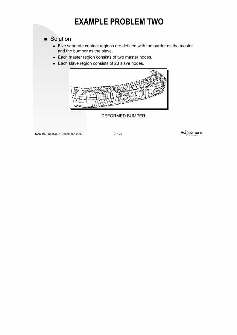
7/21/2019 Nonlinear Analysis Using MSC.nastran
http://slidepdf.com/reader/full/nonlinear-analysis-using-mscnastran 503/783
S7-74NAS 103, Section 7, December, 2003
Purpose To illustrate the use of slideline contact and nonlinear transient analysis
in bumper crash applications.
Problem Description A rigid barrier moving at 5 mph. impacts a bumber fixed at the bumper
brackets. Plot the deformed shape of the bumper after 20 msec ofcontact.
EXAMPLE PROBLEM TWO
Solution

7/21/2019 Nonlinear Analysis Using MSC.nastran
http://slidepdf.com/reader/full/nonlinear-analysis-using-mscnastran 504/783
S7-75NAS 103, Section 7, December, 2003
Solution Five separate contact regions are defined with the barrier as the master
and the bumper as the slave.
Each master region consists of two master nodes. Each slave region consists of 23 slave nodes.
DEFORMED BUMPER
WORKSHOP PROBLEMS ONE THROUGHTHREE
Purpose
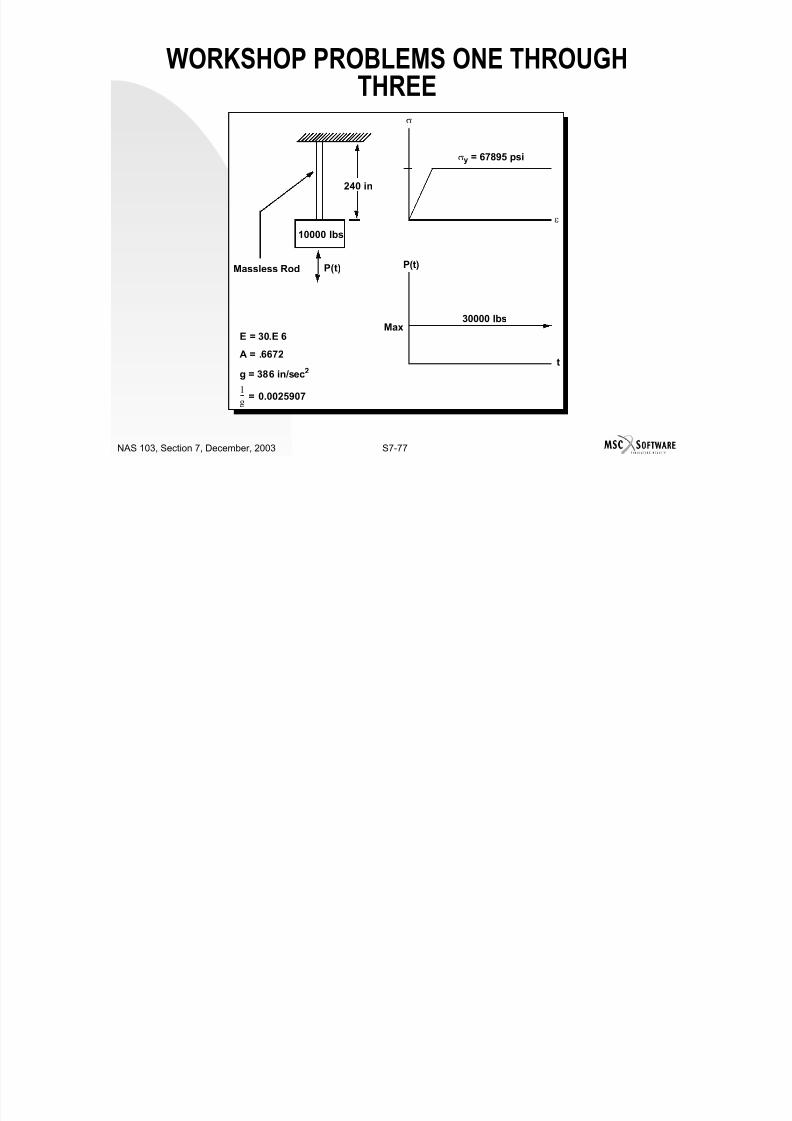
7/21/2019 Nonlinear Analysis Using MSC.nastran
http://slidepdf.com/reader/full/nonlinear-analysis-using-mscnastran 505/783
S7-76NAS 103, Section 7, December, 2003
Purpose To demonstrate the use of cold start and restart procedures for
nonlinear transient analysis (SOL 129).
Problem Description For the massless rod given below, calculate and plot (a) the rod stress
time history and (b) displacement, velocity, and acceleration time historyfor the mass. Request the output every tenth time step.
WORKSHOP PROBLEMS ONE THROUGHTHREE
σ

7/21/2019 Nonlinear Analysis Using MSC.nastran
http://slidepdf.com/reader/full/nonlinear-analysis-using-mscnastran 506/783
S7-77NAS 103, Section 7, December, 2003
P(t)
Max30000 lbs
t
10000 lbs
240 in
P(t)Massless Rod
σy = 67895 psi
ε
E = 30.E 6
A = .6672
g = 386 in/sec2
= 0.00259071
g---
WORKSHOP PROBLEMS ONE THROUGHTHREE
1 Modify the input file to perform the analysis in one
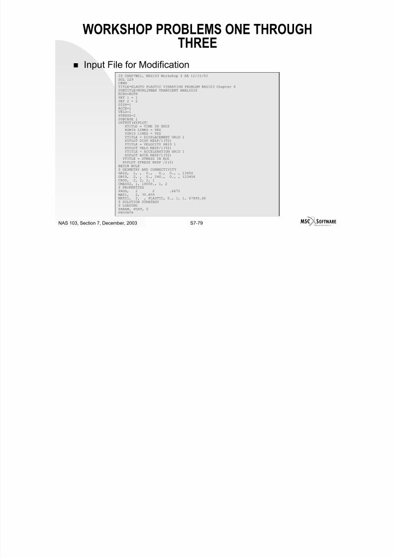
7/21/2019 Nonlinear Analysis Using MSC.nastran
http://slidepdf.com/reader/full/nonlinear-analysis-using-mscnastran 507/783
S7-78NAS 103, Section 7, December, 2003
1. Modify the input file to perform the analysis in onesubcase for a total duration of 0.3 seconds with an initialtime increment of 0.0025 seconds.
2. Modify the input file to perform the analysis in threesubcases. The duration for the first, second, and thirdsubcase is 0.125, 0.100, and 0.075 seconds,
respectively.3. Restart the analysis from the end of subcase two.
WORKSHOP PROBLEMS ONE THROUGHTHREE
Input File for Modification
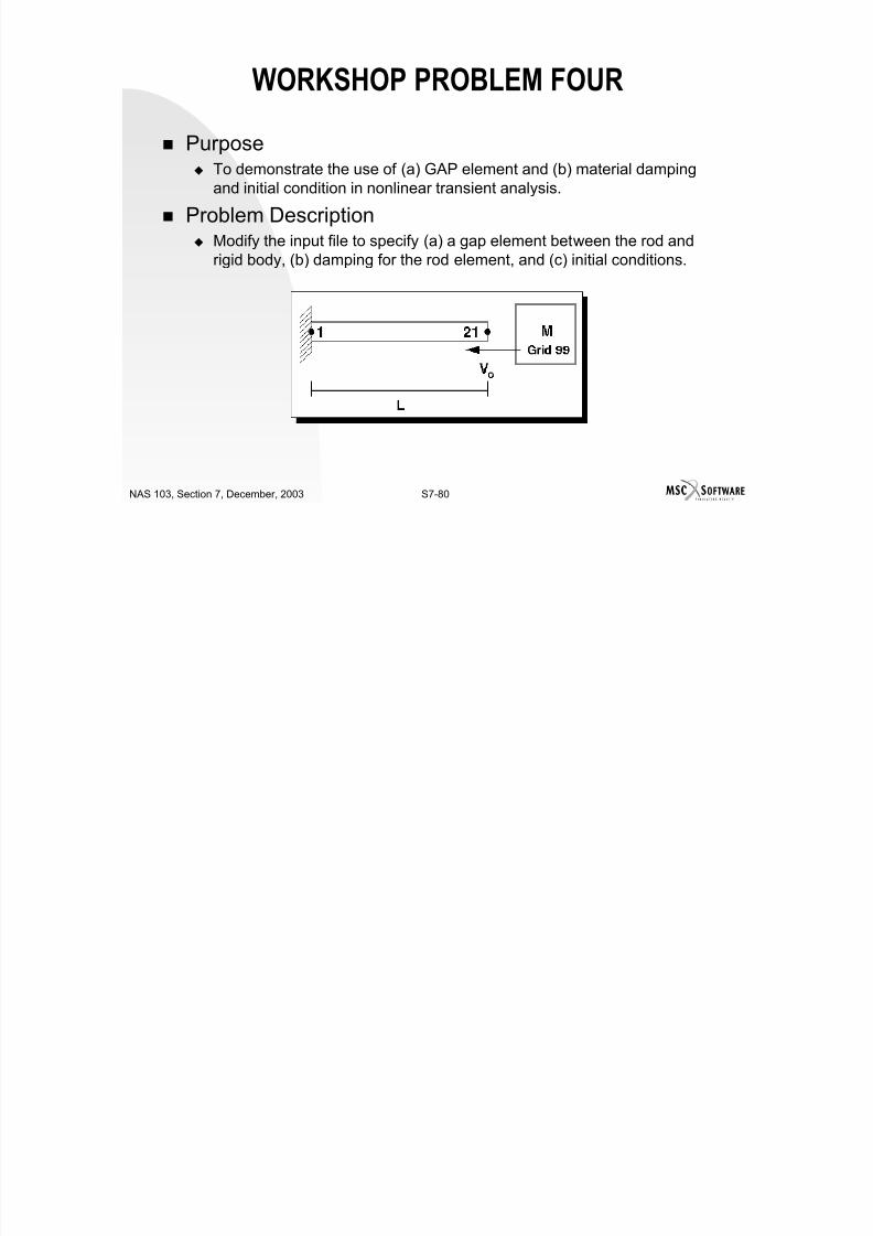
7/21/2019 Nonlinear Analysis Using MSC.nastran
http://slidepdf.com/reader/full/nonlinear-analysis-using-mscnastran 508/783
S7-79NAS 103, Section 7, December, 2003
Input File for ModificationID CHAP7WS1, NAS103 Workshop $ AR 12/15/03SOL 129CENDTITLE=ELASTO PLASTIC VIBRATION PROBLEM NAS103 Chapter 6SUBTITLE=NONLINEAR TRANSIENT ANALYSISECHO=BOTHSET 1 = 1SET 2 = 2DISP=1ACCE=1VELO=1STRESS=2SUBCASE 1OUTPUT(XYPLOT)
XTITLE = TIME IN SECSXGRID LINES = YESYGRID LINES = YES
YTITLE = DISPLACEMENT GRID 1XYPLOT DISP RESP/1(T2)YTITLE = VELOCITY GRID 1XYPLOT VELO RESP/1(T2)YTITLE = ACCELERATION GRID 1XYPLOT ACCE RESP/1(T2)YTITLE = STRESS IN RODXYPLOT STRESS RESP /2(2)
BEGIN BULK$ GEOMETRY AND CONNECTIVITYGRID, 1, , 0., 0., 0., , 13456GRID, 2, , 0., 240., 0., , 123456
CROD, 2, 2, 2, 1CMASS2, 1, 10000., 1, 2$ PROPERTIESPROD, 2 2 .6672MAT1, 2, 30.E06MATS1, 2, , PLASTIC, 0., 1, 1, 67895.68$ SOLUTION STRATEGY$ LOADINGPARAM, POST, 0ENDDATA
WORKSHOP PROBLEM FOUR
Purpose

7/21/2019 Nonlinear Analysis Using MSC.nastran
http://slidepdf.com/reader/full/nonlinear-analysis-using-mscnastran 509/783
S7-80NAS 103, Section 7, December, 2003
p To demonstrate the use of (a) GAP element and (b) material damping
and initial condition in nonlinear transient analysis.
Problem Description Modify the input file to specify (a) a gap element between the rod and
rigid body, (b) damping for the rod element, and (c) initial conditions.
WORKSHOP PROBLEM FOUR
Rod length, L = 100.m
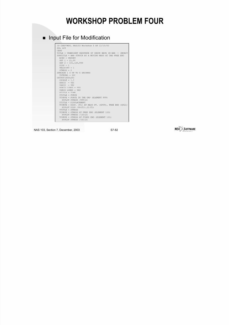
7/21/2019 Nonlinear Analysis Using MSC.nastran
http://slidepdf.com/reader/full/nonlinear-analysis-using-mscnastran 510/783
S7-81NAS 103, Section 7, December, 2003
Area of rod, A = 1.m2
Young’s modulus, E = 103 N/m2
Poisson’s ration, ν = 0.3 Mass density, ρ = 1.0 kg/m3
Mass of rod, m = ρ = AL = 10. kg
Mass of rigid body, M = 20.kg
Velocity of impact for Vo = 0.1 m/sec
Damping = 0.1% at first mode
570796 .1El L2
TT )1n2 ( =
−= ρ ω
WORKSHOP PROBLEM FOUR
Input File for Modification

7/21/2019 Nonlinear Analysis Using MSC.nastran
http://slidepdf.com/reader/full/nonlinear-analysis-using-mscnastran 511/783
S7-82NAS 103, Section 7, December, 2003
pID CHAP7WS4, NAS103 Workshop $ AR 12/15/03
SOL 129CENDTITLE = TRANSIENT RESPONSE OF SHOCK WAVE IN BAR -- IMPACT
SUBTITLE = BAR STRUCK BY A MOVING MASS AT THE FREE ENDECHO = UNSORTSET 1 = 21,99SET 2 = 101,120,899DISP = 1VELOCITY = 1
STRESS = 2SUBCASE 1 $ UP TO 6 SECONDSTSTEPNL = 200
OUTPUT(XYPLOT)
CSCALE = 1.5XAXIS = YESYAXIS = YESXGRID LINES = YES
YGRID LINES = YESXTITLE = TIMEYTITLE = FORCETCURVE = FORCE IN THE GAP (ELEMENT 899)XYPLOT STRESS /899(2)
YTITLE = DISPLACEMENT
TCURVE = DISP. (T1) AT MASS PT. (GP99), FREE END (GP21)XYPLOT DISP /99(T1),21(T1)YTITLE = STRESS
TCURVE = STRESS AT FREE END (ELEMENT 120)XYPLOT STRESS /120(2)
TCURVE = STRESS AT FIXED END (ELEMENT 101)XYPLOT STRESS /101(2)
WORKSHOP PROBLEM FOUR
Input File for Modification (cont.)
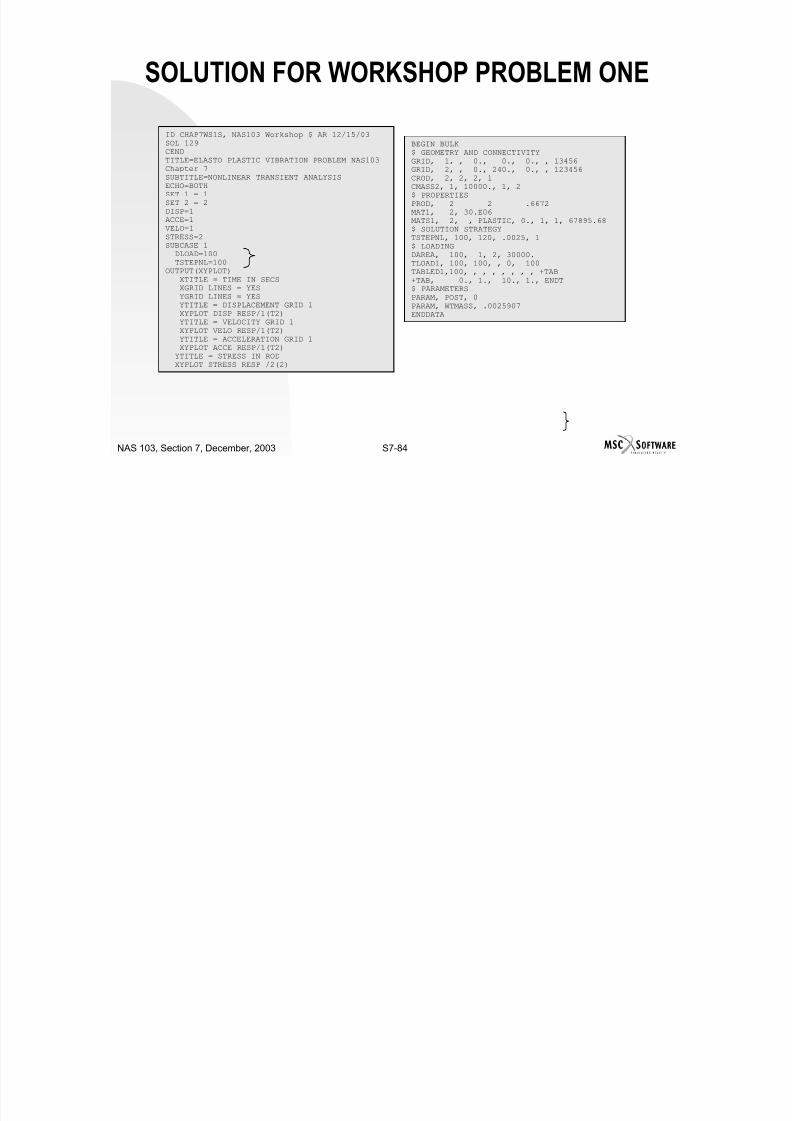
7/21/2019 Nonlinear Analysis Using MSC.nastran
http://slidepdf.com/reader/full/nonlinear-analysis-using-mscnastran 512/783
S7-83NAS 103, Section 7, December, 2003
BEGIN BULK
$ GEOMETRY
GRDSET, , , , , , , 23456
GRID, 1, ,0., 0., 0., , 123456
GRID, 2, ,5., 0., 0.
=,*1,=,*5.,== $
=18
GRID, 99, , 100., 0., 0.
$ ELEMENT CONNECTIVITY
CONROD, 101, 1, 2, 100, 1.
=,*1,*1,*1,== $
=18
$ MATERIAL PROPERTIES
CONM2, 999, 99, , 20.
$ GAP ELEMENT CONNEVTIVITY
$ GAP ELEMENT PROPERTIES
$ INITIAL CONDITIONS
$ PARAMETERS
param, post, 0
PARAM, COUPMASS, 1
$ SOLUTION STRATEGY
TSTEPNL 200 600 .01 1
$
ENDDATA
SOLUTION FOR WORKSHOP PROBLEM ONE
ID CHAP7WS1S, NAS103 Workshop $ AR 12/15/03SOL 129 BEGIN BULK

7/21/2019 Nonlinear Analysis Using MSC.nastran
http://slidepdf.com/reader/full/nonlinear-analysis-using-mscnastran 513/783
S7-84NAS 103, Section 7, December, 2003
SOL 129CENDTITLE=ELASTO PLASTIC VIBRATION PROBLEM NAS103Chapter 7SUBTITLE=NONLINEAR TRANSIENT ANALYSISECHO=BOTH
SET 1 = 1SET 2 = 2DISP=1ACCE=1VELO=1STRESS=2SUBCASE 1
DLOAD=100TSTEPNL=100
OUTPUT(XYPLOT)
XTITLE = TIME IN SECSXGRID LINES = YESYGRID LINES = YESYTITLE = DISPLACEMENT GRID 1XYPLOT DISP RESP/1(T2)YTITLE = VELOCITY GRID 1XYPLOT VELO RESP/1(T2)YTITLE = ACCELERATION GRID 1XYPLOT ACCE RESP/1(T2)YTITLE = STRESS IN ROD
XYPLOT STRESS RESP /2(2)
BEGIN BULK$ GEOMETRY AND CONNECTIVITYGRID, 1, , 0., 0., 0., , 13456GRID, 2, , 0., 240., 0., , 123456CROD, 2, 2, 2, 1CMASS2, 1, 10000., 1, 2
$ PROPERTIESPROD, 2 2 .6672MAT1, 2, 30.E06MATS1, 2, , PLASTIC, 0., 1, 1, 67895.68$ SOLUTION STRATEGYTSTEPNL, 100, 120, .0025, 1$ LOADINGDAREA, 100, 1, 2, 30000.TLOAD1, 100, 100, , 0, 100TABLED1,100, , , , , , , , +TAB
+TAB, 0., 1., 10., 1., ENDT$ PARAMETERSPARAM, POST, 0PARAM, WTMASS, .0025907ENDDATA
SOLUTION FOR WORKSHOP PROBLEM ONE
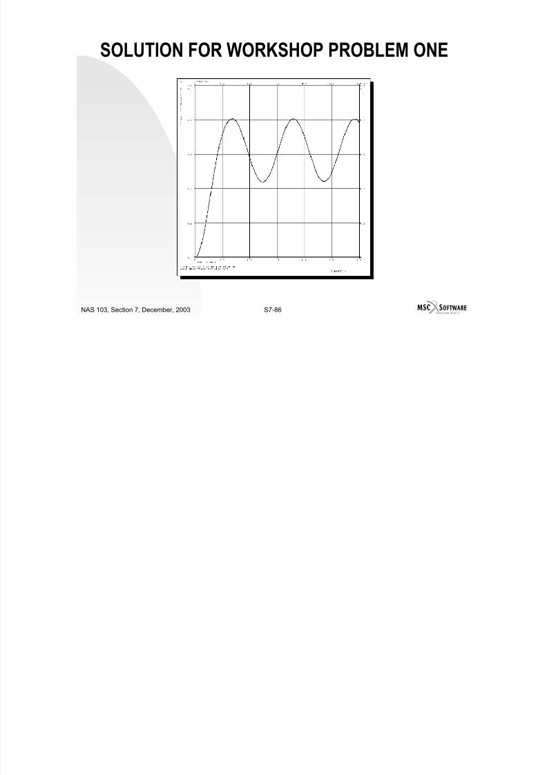
7/21/2019 Nonlinear Analysis Using MSC.nastran
http://slidepdf.com/reader/full/nonlinear-analysis-using-mscnastran 514/783
S7-85NAS 103, Section 7, December, 2003
SOLUTION FOR WORKSHOP PROBLEM ONE
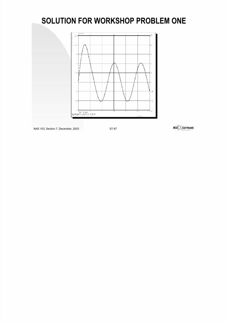
7/21/2019 Nonlinear Analysis Using MSC.nastran
http://slidepdf.com/reader/full/nonlinear-analysis-using-mscnastran 515/783
S7-86NAS 103, Section 7, December, 2003
SOLUTION FOR WORKSHOP PROBLEM ONE
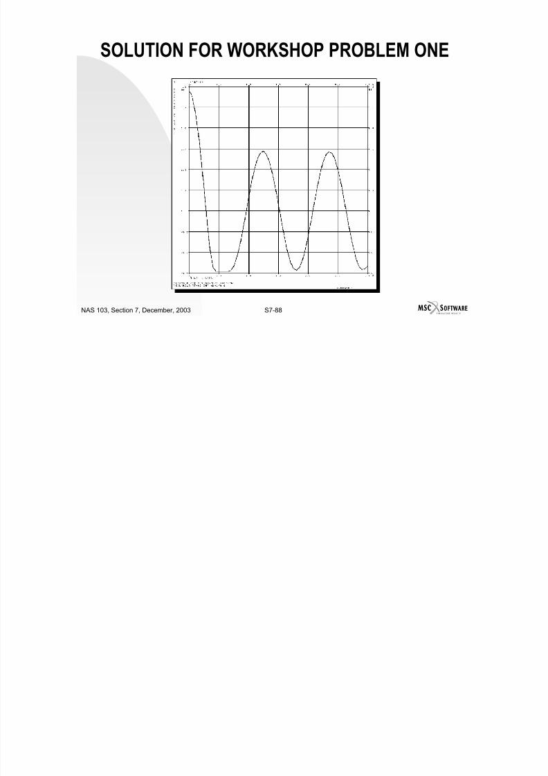
7/21/2019 Nonlinear Analysis Using MSC.nastran
http://slidepdf.com/reader/full/nonlinear-analysis-using-mscnastran 516/783
S7-87NAS 103, Section 7, December, 2003
SOLUTION FOR WORKSHOP PROBLEM ONE

7/21/2019 Nonlinear Analysis Using MSC.nastran
http://slidepdf.com/reader/full/nonlinear-analysis-using-mscnastran 517/783
S7-88NAS 103, Section 7, December, 2003
SOLUTION FOR WORKSHOP PROBLEM TWO
ID CHAP7WS2S, NAS103 Workshop $ AR 12/15/03SOL 129CENDTITLE=ELASTO PLASTIC VIBRATION PROBLEM NAS103Chapter 7
BEGIN BULK$ GEOMETRY AND CONNECTIVITY

7/21/2019 Nonlinear Analysis Using MSC.nastran
http://slidepdf.com/reader/full/nonlinear-analysis-using-mscnastran 518/783
S7-89NAS 103, Section 7, December, 2003
Chapter 7SUBTITLE=NONLINEAR TRANSIENT ANALYSISECHO=BOTHSET 1 = 1SET 2 = 2DISP=1ACCE=1VELO=1STRESS=2SUBCASE 1DLOAD=100TSTEPNL=100
SUBCASE 2DLOAD=100TSTEPNL=200
SUBCASE 3DLOAD=100TSTEPNL=300
OUTPUT(XYPLOT)XTITLE = TIME IN SECSXGRID LINES = YESYGRID LINES = YESYTITLE = DISPLACEMENT GRID 1XYPLOT DISP RESP/1(T2)YTITLE = VELOCITY GRID 1XYPLOT VELO RESP/1(T2)YTITLE = ACCELERATION GRID 1XYPLOT ACCE RESP/1(T2)YTITLE = STRESS IN RODXYPLOT STRESS RESP /2(2)
GRID, 1, , 0., 0., 0., , 13456GRID, 2, , 0., 240., 0., , 123456CROD, 2, 2, 2, 1CMASS2, 1, 10000., 1, 2$ PROPERTIES
PROD, 2 2 .6672MAT1, 2, 30.E06MATS1, 2, , PLASTIC, 0., 1, 1, 67895.68$ SOLUTION STRATEGYTSTEPNL, 100, 50, .0025, 1TSTEPNL, 200, 40, .0025, 1TSTEPNL, 300, 30, .0025, 1$ LOADINGDAREA, 100, 1, 2, 30000.TLOAD1, 100, 100, , 0, 100
TABLED1,100, , , , , , , , +TAB+TAB, 0., 1., 10., 1., ENDT$ PARAMETERSPARAM, POST, 0PARAM, WTMASS, .0025907ENDDATA
SOLUTION FOR WORKSHOP PROBLEMTHREE
RESTART,VERSION=1,KEEPASSIGN MASTER='chap7_ws_2s.MASTER'ID CHAP7_WS_3S, NAS103 Workshop $ AR 12/15/03SOL 129CEND

7/21/2019 Nonlinear Analysis Using MSC.nastran
http://slidepdf.com/reader/full/nonlinear-analysis-using-mscnastran 519/783
S7-90NAS 103, Section 7, December, 2003
CENDTITLE=ELASTO PLASTIC VIBRATION PROBLEM NAS103 Chapter7SUBTITLE=NONLINEAR TRANSIENT ANALYSISECHO=BOTH$ INITIAL STATE FOR RESTART
PARAM,LOOPID,2PARAM,STIME,0.225$SET 1 = 1SET 2 = 2DISP=1ACCE=1VELO=1STRESS=2SUBCASE 1DLOAD=100TSTEPNL=100
SUBCASE 2DLOAD=100TSTEPNL=200
SUBCASE 3DLOAD=100TSTEPNL=300
OUTPUT(XYPLOT)XTITLE = TIME IN SECSXGRID LINES = YESYGRID LINES = YESYTITLE = DISPLACEMENT GRID 1XYPLOT DISP RESP/1(T2)
YTITLE = VELOCITY GRID 1XYPLOT VELO RESP/1(T2)YTITLE = ACCELERATION GRID 1XYPLOT ACCE RESP/1(T2)YTITLE = STRESS IN RODXYPLOT STRESS RESP /2(2)
BEGIN BULKENDDATA
SOLUTION FOR WORKSHOP PROBLEM FOUR
ID CHAP7WS4S, NAS103 Workshop $ AR 12/15/03SOL 129
CEND
TITLE = TRANSIENT RESPONSE OF SHOCK WAVE IN BAR -- IMPACT
SUBTITLE = BAR STRUCK BY A MOVING MASS AT THE FREE END

7/21/2019 Nonlinear Analysis Using MSC.nastran
http://slidepdf.com/reader/full/nonlinear-analysis-using-mscnastran 520/783
S7-91NAS 103, Section 7, December, 2003
ECHO = UNSORT
SET 1 = 21,99
SET 2 = 101,120,899
DISP = 1
VELOCITY = 1
STRESS = 2SUBCASE 1 $ UP TO 6 SECONDS
IC = 1
TSTEPNL = 200
OUTPUT(XYPLOT)
CSCALE = 1.5
XAXIS = YES
YAXIS = YES
XGRID LINES = YES
YGRID LINES = YES
XTITLE = TIMEYTITLE = FORCE
TCURVE = FORCE IN THE GAP (ELEMENT 899)
XYPLOT STRESS /899(2)
YTITLE = DISPLACEMENT
TCURVE = DISP. (T1) AT MASS PT. (GP99), FREE END (GP21)
XYPLOT DISP /99(T1),21(T1)
YTITLE = STRESS
TCURVE = STRESS AT FREE END (ELEMENT 120)
XYPLOT STRESS /120(2)
TCURVE = STRESS AT FIXED END (ELEMENT 101)
XYPLOT STRESS /101(2)
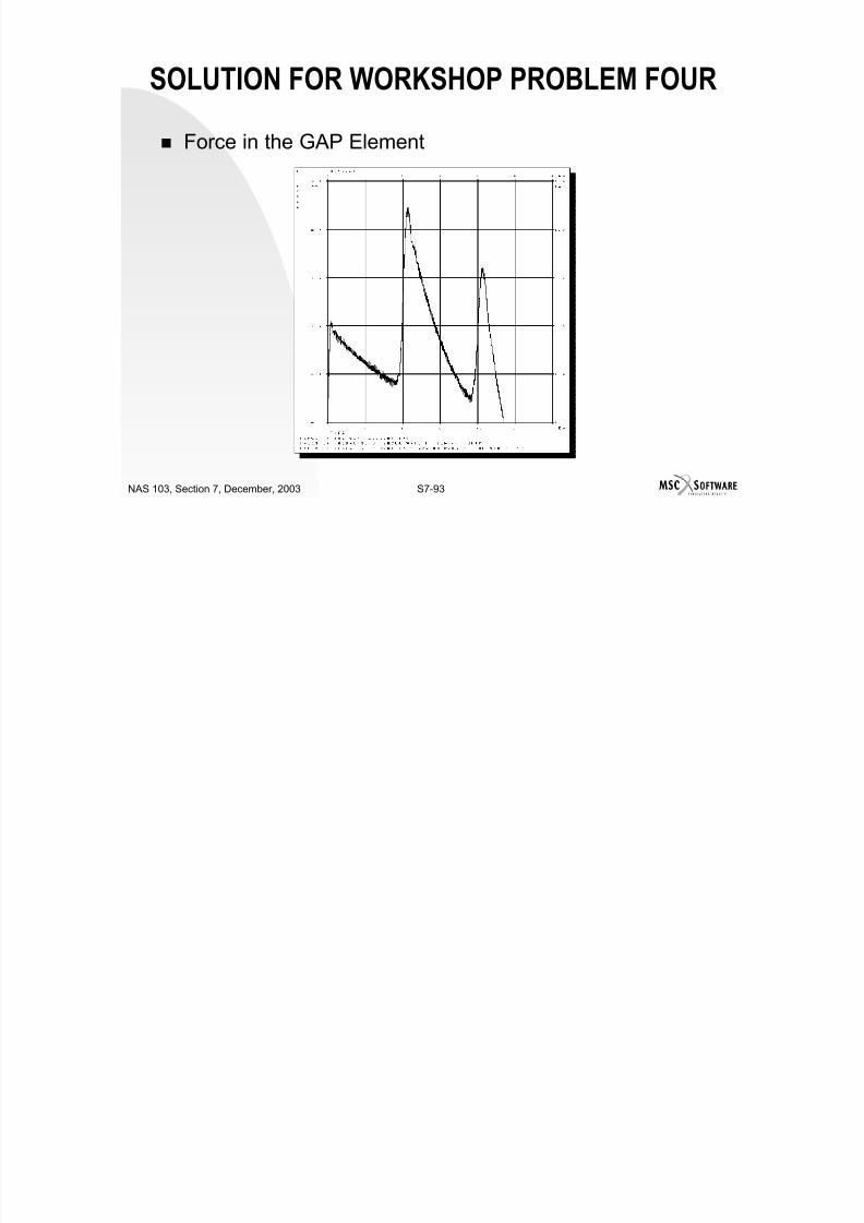
7/21/2019 Nonlinear Analysis Using MSC.nastran
http://slidepdf.com/reader/full/nonlinear-analysis-using-mscnastran 521/783
SOLUTION FOR WORKSHOP PROBLEM FOUR
Force in the GAP Element
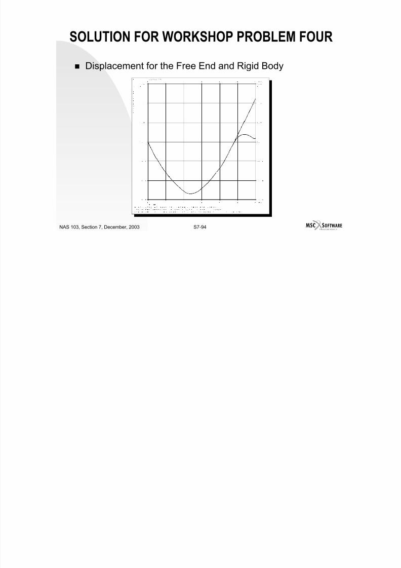
7/21/2019 Nonlinear Analysis Using MSC.nastran
http://slidepdf.com/reader/full/nonlinear-analysis-using-mscnastran 522/783
S7-93NAS 103, Section 7, December, 2003
SOLUTION FOR WORKSHOP PROBLEM FOUR
Displacement for the Free End and Rigid Body
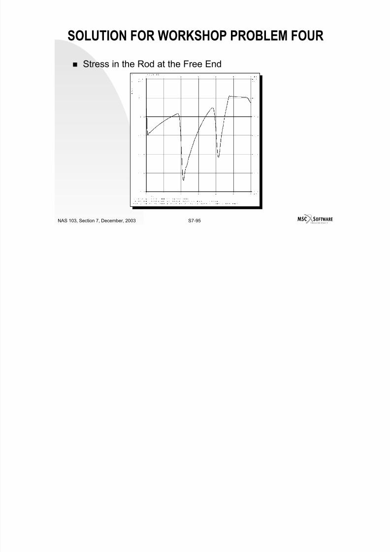
7/21/2019 Nonlinear Analysis Using MSC.nastran
http://slidepdf.com/reader/full/nonlinear-analysis-using-mscnastran 523/783
S7-94NAS 103, Section 7, December, 2003
SOLUTION FOR WORKSHOP PROBLEM FOUR
Stress in the Rod at the Free End
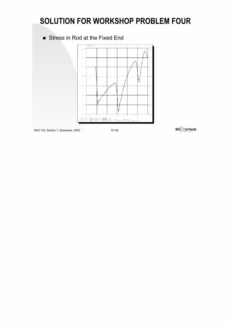
7/21/2019 Nonlinear Analysis Using MSC.nastran
http://slidepdf.com/reader/full/nonlinear-analysis-using-mscnastran 524/783
S7-95NAS 103, Section 7, December, 2003
SOLUTION FOR WORKSHOP PROBLEM FOUR
Stress in Rod at the Fixed End

7/21/2019 Nonlinear Analysis Using MSC.nastran
http://slidepdf.com/reader/full/nonlinear-analysis-using-mscnastran 525/783
S7-96NAS 103, Section 7, December, 2003

7/21/2019 Nonlinear Analysis Using MSC.nastran
http://slidepdf.com/reader/full/nonlinear-analysis-using-mscnastran 526/783
S8-1NAS 103, Section 8, December 2003
SECTION 8
NONLINEAR ANALYSIS WITHSUPERELEMENTS
7/21/2019 Nonlinear Analysis Using MSC.nastran
http://slidepdf.com/reader/full/nonlinear-analysis-using-mscnastran 527/783
S8-2NAS 103, Section 8, December 2003
TABLE OF CONTENTS
Page Advantage Of Superelement Analysis 8-4Typical Aircraft Superelement Arrangement 8-6
7/21/2019 Nonlinear Analysis Using MSC.nastran
http://slidepdf.com/reader/full/nonlinear-analysis-using-mscnastran 528/783
S8-3NAS 103, Section 8, December 2003
Typical Aircraft Superelement Arrangement 8-6How Are Superelements Defined In MSC.Nastran? 8-7
Grid Point Partitioning 8-8Interior Versus Exterior 8-10Element Partitioning 8-11Solution Terminology 8-12Super Command 8-14Superelement Example Input 8-16Nonlinear Analysis Features 8-17Hierarchy Of Load Data 8-20Example Of Case Control With Upstream Loads 8-21
Example Of Bulk Data To Specify Upstream Loads 8-22Workshop Problem 1 8-23Solution For Workshop Problem 1 8-28
ADVANTAGE OF SUPERELEMENT ANALYSIS
Large problems (i.e., allows solving problems thatexceed your hardware capabilities).

7/21/2019 Nonlinear Analysis Using MSC.nastran
http://slidepdf.com/reader/full/nonlinear-analysis-using-mscnastran 529/783
S8-4NAS 103, Section 8, December 2003
Less CPU or wall clock time per run (reduced risk since
each superelement may be processed individually). Partial redesign requires only partial solution (cost). Allows more control of resource usage. Partitioned input desirable.
Organization Repeated components
Partitioned output desirable. Organization
Comprehension Components may be modeled by subcontractors.
ADVANTAGE OF SUPERELEMENT ANALYSIS
Multi-step reduction for dynamic analysis.
Zooming (or global-local analysis).
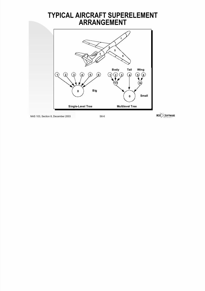
7/21/2019 Nonlinear Analysis Using MSC.nastran
http://slidepdf.com/reader/full/nonlinear-analysis-using-mscnastran 530/783
S8-5NAS 103, Section 8, December 2003
g ( g y )
Allows for efficient configuration studies (“What if...”).
TYPICAL AIRCRAFT SUPERELEMENTARRANGEMENT
1
7/21/2019 Nonlinear Analysis Using MSC.nastran
http://slidepdf.com/reader/full/nonlinear-analysis-using-mscnastran 531/783
S8-6NAS 103, Section 8, December 2003
2
5
63
4
1 2 3 4 5 6
0
1 2 3 4 5 6
0
56
Single-Level Tree Multilevel Tree
Small
Big
Body Tail Wing
123
HOW ARE SUPERELEMENTS DEFINED INMSC.NASTRAN?
Superelements are identified using numbers (SEID). Each superelement (SEID > 0) is defined with its own set
f id l t t i t l d t

7/21/2019 Nonlinear Analysis Using MSC.nastran
http://slidepdf.com/reader/full/nonlinear-analysis-using-mscnastran 532/783
S8-7NAS 103, Section 8, December 2003
of grids, elements, constraints, loads, etc. Interior grid points are assigned (partitioned) to a superelement by the
user. Exterior grid points, elements, loads, and constraints are automatically
partitioned by the program based on interior grid point assignments.
The residual structure is a superelement that contains
grid points, elements, etc., which are not assigned to anyother superelement. Last superelement (SEID = 0) to be processed. Superelement on which the assembly analysis (nonlinear, transient
response, frequency response, buckling, system modes, etc.) isperformed.
A superelement may also be defined as an image of asuperelement or obtained from outside MSC.NASTRAN.
GRID POINT PARTITIONING
Bulk Data Entries
SEIDETC.GIDGRID
10987654321

7/21/2019 Nonlinear Analysis Using MSC.nastran
http://slidepdf.com/reader/full/nonlinear-analysis-using-mscnastran 533/783
S8-8NAS 103, Section 8, December 2003
Only interior points need to be defined.
247GRID
57THRU470SESET
G2“THRU”G1SEIDSESET
10987654321
Superelements are identifiedby an integer
GRID POINT PARTITIONING
SESET takes precedence over GRID. For the example shown above, Grid Point 47 will belong to the residual
structure (SEID=0)

7/21/2019 Nonlinear Analysis Using MSC.nastran
http://slidepdf.com/reader/full/nonlinear-analysis-using-mscnastran 534/783
S8-9NAS 103, Section 8, December 2003
structure (SEID=0).
Elements, constraints, loads, etc., are automaticallypartitioned.
Points not assigned belong to the residual structure bydefault. A model with no grid point assignments is
defined as a residual structure-only model.
INTERIOR VERSUS EXTERIOR
A grid point assigned to a superelement by the user isinterior to that superelement.
Th i d d fi t i t f id i t
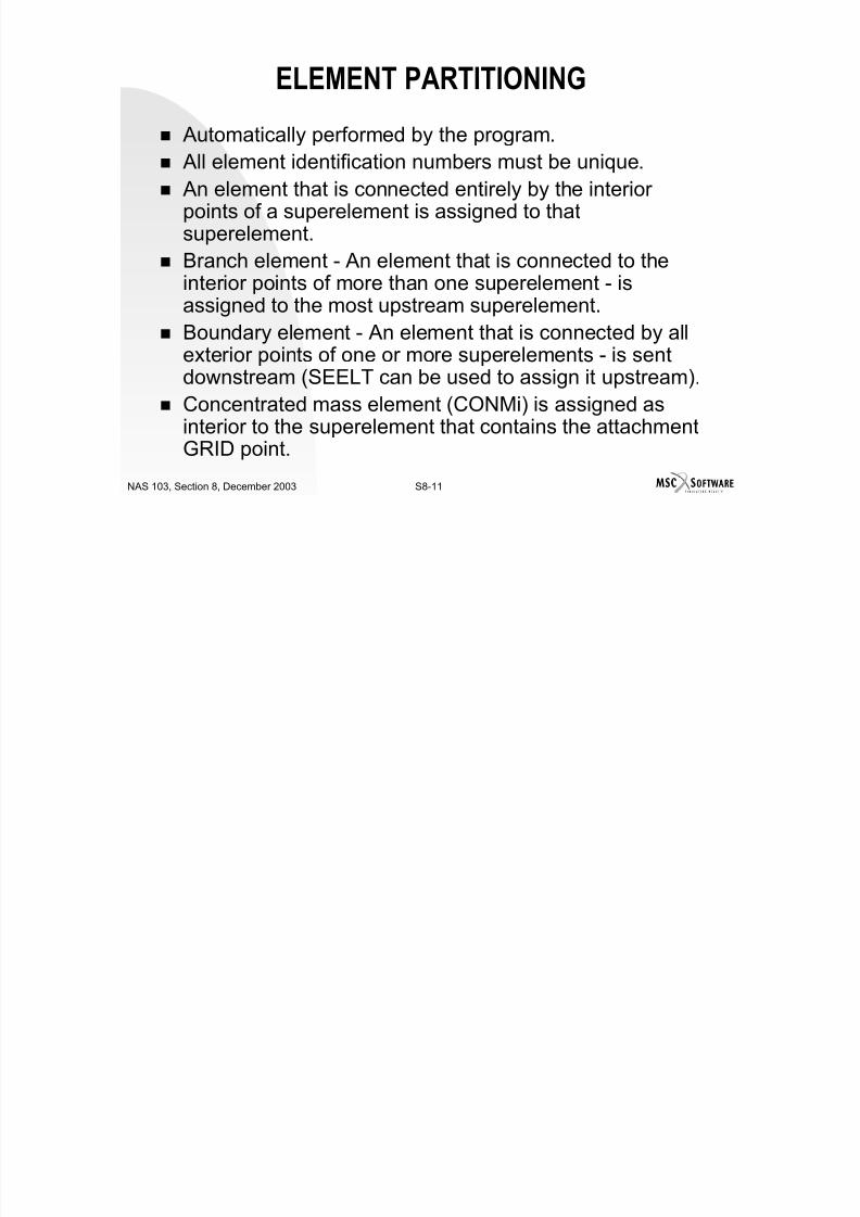
7/21/2019 Nonlinear Analysis Using MSC.nastran
http://slidepdf.com/reader/full/nonlinear-analysis-using-mscnastran 535/783
S8-10NAS 103, Section 8, December 2003
The processing order defines exterior sets of grid points
for each superelement. A grid point that is connected to a superelement and is
interior to a downstream superelement is exterior to theupstream superelement.
Scalar points are interior only to the residual structurebut may be exterior to any number of superelements.
ELEMENT PARTITIONING
Automatically performed by the program. All element identification numbers must be unique.
An element that is connected entirel b the interior

7/21/2019 Nonlinear Analysis Using MSC.nastran
http://slidepdf.com/reader/full/nonlinear-analysis-using-mscnastran 536/783
S8-11NAS 103, Section 8, December 2003
An element that is connected entirely by the interior
points of a superelement is assigned to thatsuperelement. Branch element - An element that is connected to the
interior points of more than one superelement - is
assigned to the most upstream superelement. Boundary element - An element that is connected by all
exterior points of one or more superelements - is sentdownstream (SEELT can be used to assign it upstream).
Concentrated mass element (CONMi) is assigned asinterior to the superelement that contains the attachmentGRID point.
SOLUTION TERMINOLOGY
Superelement matrix generation “SEMG” Generate structural matrices (KGG, KJJ), MJJ, BJJ.
Enforced displacements rigid elements MPCs check singularities

7/21/2019 Nonlinear Analysis Using MSC.nastran
http://slidepdf.com/reader/full/nonlinear-analysis-using-mscnastran 537/783
S8-12NAS 103, Section 8, December 2003
Enforced displacements, rigid elements, MPCs, check singularities.
Superelement load generation “SELG” (statics only) Generate load matrices (PG, PJ).
Superelement stiffness (K) reduction “SEKR” (stiffnessonly)
Superelement mass (and damping) reduction “SEMR” Assemble upstreams.
Reduce to (boundary exterior) points.
Superelement load reduction “SELR” Loads, mass or damping.
Float downstream to assemble, reduce.
SOLUTION TERMINOLOGY
Superelement data recovery “SEDR” Expand boundary displacements.
Compute internal loads stresses element strain energy etc

7/21/2019 Nonlinear Analysis Using MSC.nastran
http://slidepdf.com/reader/full/nonlinear-analysis-using-mscnastran 538/783
S8-13NAS 103, Section 8, December 2003
Compute internal loads, stresses, element strain energy, etc.
SUPER COMMAND
Partitions (assigns) a subcase to a superelement(s).
Associates a superelement(s) with requests forparameters loads constraints and output

7/21/2019 Nonlinear Analysis Using MSC.nastran
http://slidepdf.com/reader/full/nonlinear-analysis-using-mscnastran 539/783
S8-14NAS 103, Section 8, December 2003
parameters, loads, constraints, and output.
Subcase is required for each superelement and for eachload condition.
If the Case Control Section does not contain a SUPER
command, then loads, constraints, and output requestsare applied to the residual structure only.
The SUPER command may reference a superelement ora SET of superelements. Note: The SET ID must be unique with respect to any superelement
IDs.
SUPER COMMAND
Examples:SUPER = ALL
or but
SET 1 = 10, 20, 0 SET 10 = 10, 20, 0

7/21/2019 Nonlinear Analysis Using MSC.nastran
http://slidepdf.com/reader/full/nonlinear-analysis-using-mscnastran 540/783
S8-15NAS 103, Section 8, December 2003
Form of SUPER command
SUPER = i,jwhere i = superelement ID or set of superelements j= load sequence number (a counter on loading conditions)
The load sequence number for a superelement cannot be greaterthan the number of loading conditions for the residual structure (seethe MSC.NASTRAN Quick Reference Guide).
The appropriate SE_ _ = n commands must also appear above thesubcase level.
SUPER = 1 (SET) SUPER = 10 (SEID)
or
Defaults differently than other entries.
SUPER = 10
SUPERELEMENT EXAMPLE INPUT
P
10 302515 2016 19 21 24 26 29
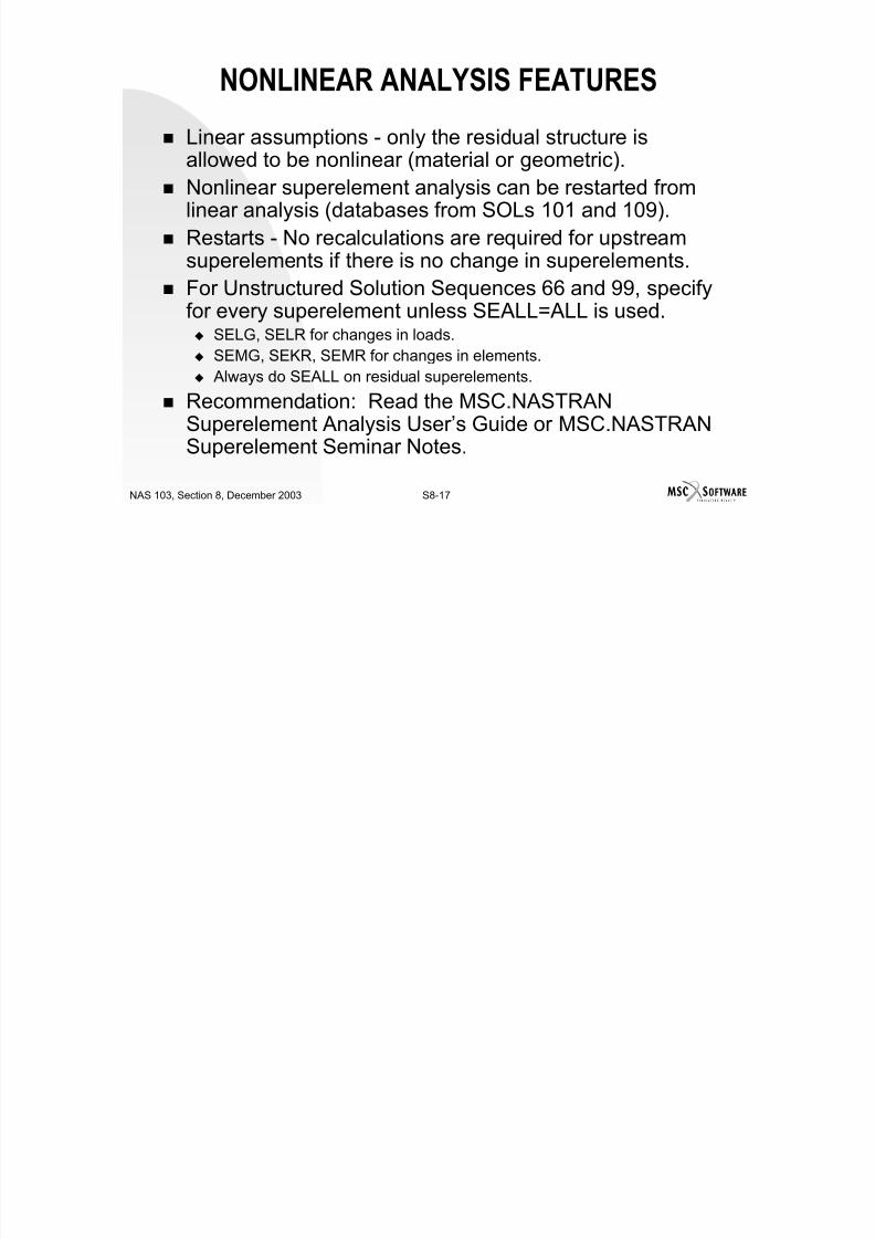
7/21/2019 Nonlinear Analysis Using MSC.nastran
http://slidepdf.com/reader/full/nonlinear-analysis-using-mscnastran 541/783
S8-16NAS 103, Section 8, December 2003
Case Control:SEALL = ALL
SUPER = ALL Bulk Data:
SESET, 1, 16, THRU, 19
SESET, 2, 21, THRU, 24
SESET, 3, 26, THRU, 29
SEID = 1 SEID = 2 SEID = 3
NONLINEAR ANALYSIS FEATURES
Linear assumptions - only the residual structure isallowed to be nonlinear (material or geometric).
Nonlinear superelement analysis can be restarted from

7/21/2019 Nonlinear Analysis Using MSC.nastran
http://slidepdf.com/reader/full/nonlinear-analysis-using-mscnastran 542/783
S8-17NAS 103, Section 8, December 2003
p ylinear analysis (databases from SOLs 101 and 109).
Restarts - No recalculations are required for upstreamsuperelements if there is no change in superelements.
For Unstructured Solution Sequences 66 and 99, specify
for every superelement unless SEALL=ALL is used. SELG, SELR for changes in loads. SEMG, SEKR, SEMR for changes in elements. Always do SEALL on residual superelements.
Recommendation: Read the MSC.NASTRANSuperelement Analysis User’s Guide or MSC.NASTRANSuperelement Seminar Notes.
NONLINEAR ANALYSIS FEATURES
Load vectors for the upstream elements must begenerated before the nonlinear solutions.
Case Control command SUPER is used to partition the

7/21/2019 Nonlinear Analysis Using MSC.nastran
http://slidepdf.com/reader/full/nonlinear-analysis-using-mscnastran 543/783
S8-18NAS 103, Section 8, December 2003
pproper subcase to a superelement.
All the subcases should include the SUPER command(default, SUPER=0) except when SUPER=ALL isspecified above the subcases.
Case Control command LOADSET selects LSEQ loads. Only one LOADSET may appear in Case Control and
must be above all the subcases. Bulk Data CLOAD entry is designed to apply static loads
to upstream superelements by combining loads definedin LSEQ.
NONLINEAR ANALYSIS FEATURES
Case Control command CLOAD must be specified in theresidual solution subcases to have loads on thesuperelements.
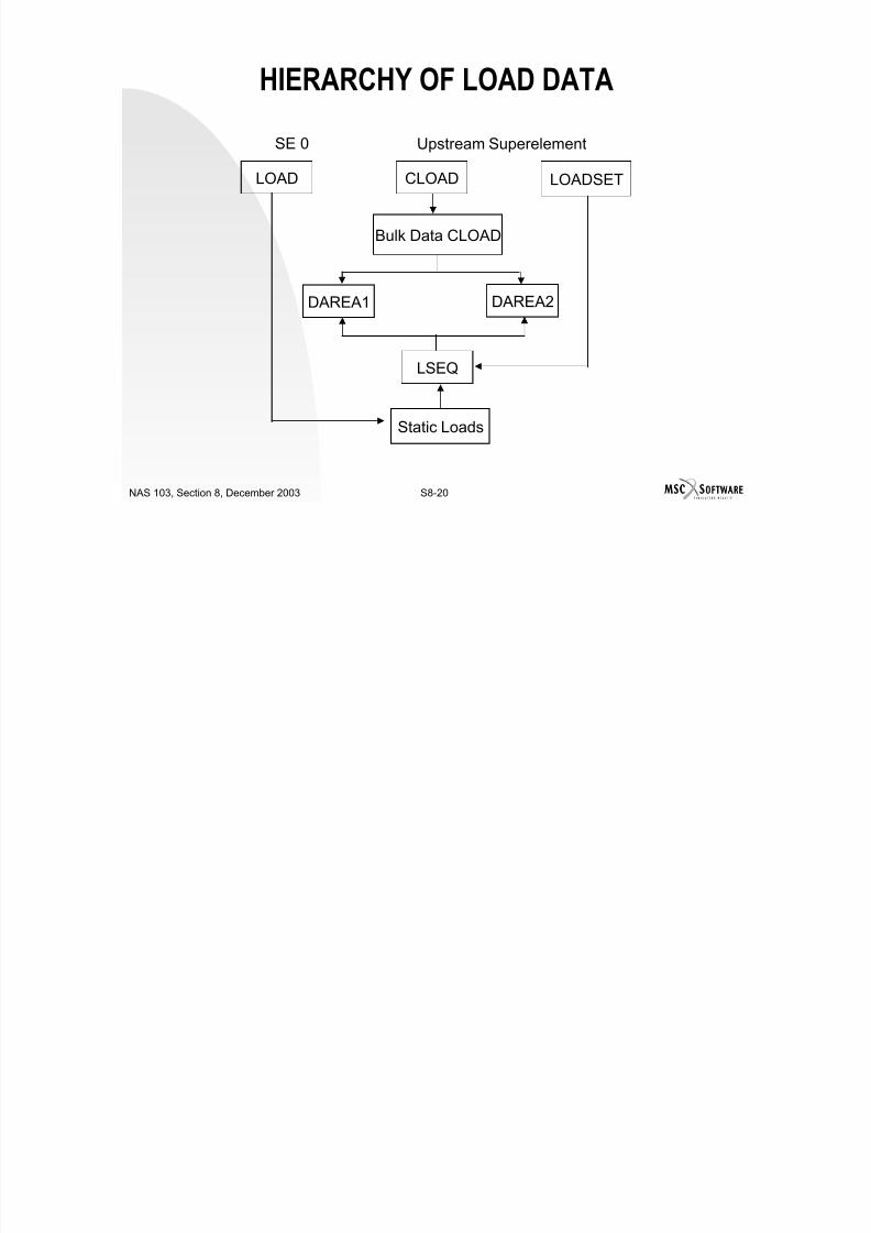
7/21/2019 Nonlinear Analysis Using MSC.nastran
http://slidepdf.com/reader/full/nonlinear-analysis-using-mscnastran 544/783
S8-19NAS 103, Section 8, December 2003
p
The Case Control command CLOAD must be specifiedin all the subcases to have data recovery forsuperelements.
Usual static load entries (LOAD, FORCE, etc.) applied tothe upstream superelements cannot be directlyreferenced by a Case Control command LOAD.
Any loads which are referenced by a CLOAD entry
should not be again referenced by a LOAD entry,otherwise, the load will be doubled, e.g., GRAV, TEMP.
HIERARCHY OF LOAD DATA
LOAD CLOAD LOADSET
SE 0 Upstream Superelement
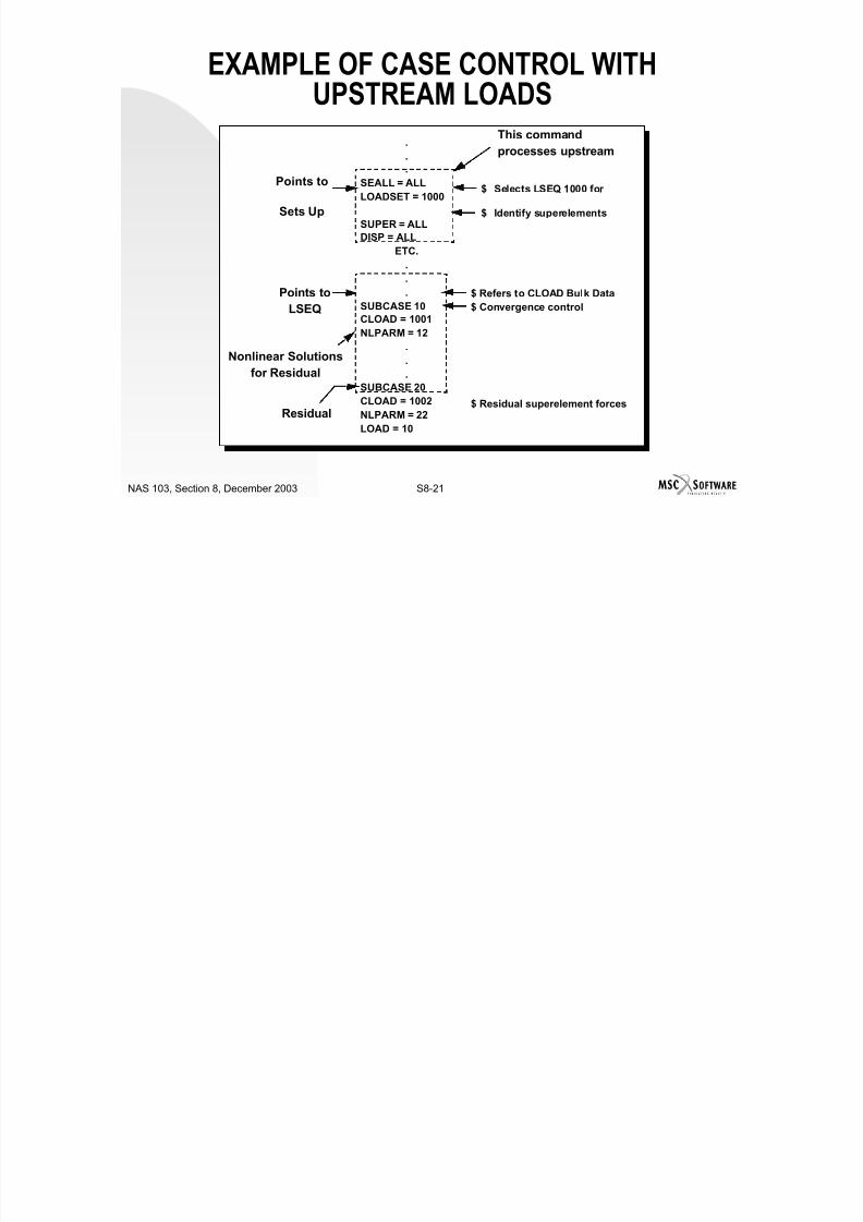
7/21/2019 Nonlinear Analysis Using MSC.nastran
http://slidepdf.com/reader/full/nonlinear-analysis-using-mscnastran 545/783
S8-20NAS 103, Section 8, December 2003
Bulk Data CLOAD
DAREA2DAREA1
LSEQ
Static Loads
EXAMPLE OF CASE CONTROL WITHUPSTREAM LOADS
.
.
.
SEALL = ALL
LOADSET = 1000$ Selects LSEQ 1000 for
This command
processes upstream
Points to
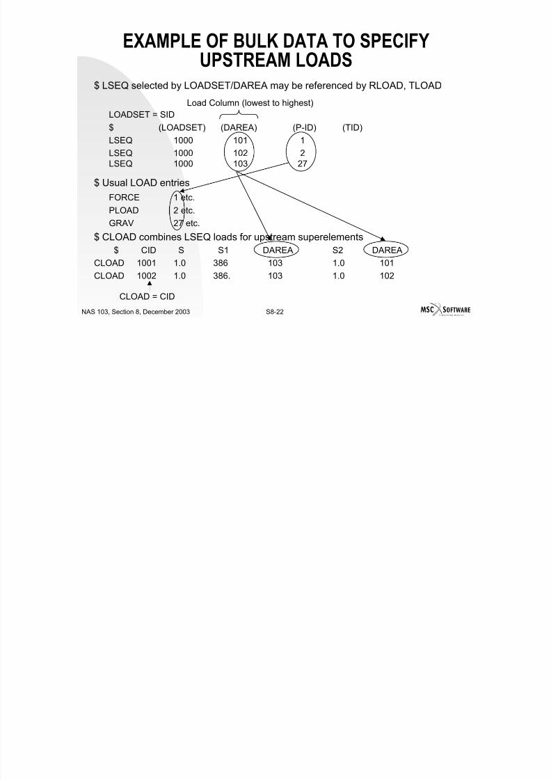
7/21/2019 Nonlinear Analysis Using MSC.nastran
http://slidepdf.com/reader/full/nonlinear-analysis-using-mscnastran 546/783
S8-21NAS 103, Section 8, December 2003
LOADSET 1000
SUPER = ALLDISP = ALL
ETC.
.
.
.
SUBCASE 10
CLOAD = 1001
NLPARM = 12
.
.
.
SUBCASE 20
CLOAD = 1002NLPARM = 22
LOAD = 10
$ Identify superelementsSets Up
$ Refers to CLOAD Bulk Data
$ Convergence control
Nonlinear Solutions
for Residual
Points to
LSEQ
Residual $ Residual superelement forces
EXAMPLE OF BULK DATA TO SPECIFYUPSTREAM LOADS
$ LSEQ selected by LOADSET/DAREA may be referenced by RLOAD, TLOAD
LOADSET = SID
$ (LOADSET) (DAREA) (P-ID) (TID)
Load Column (lowest to highest)
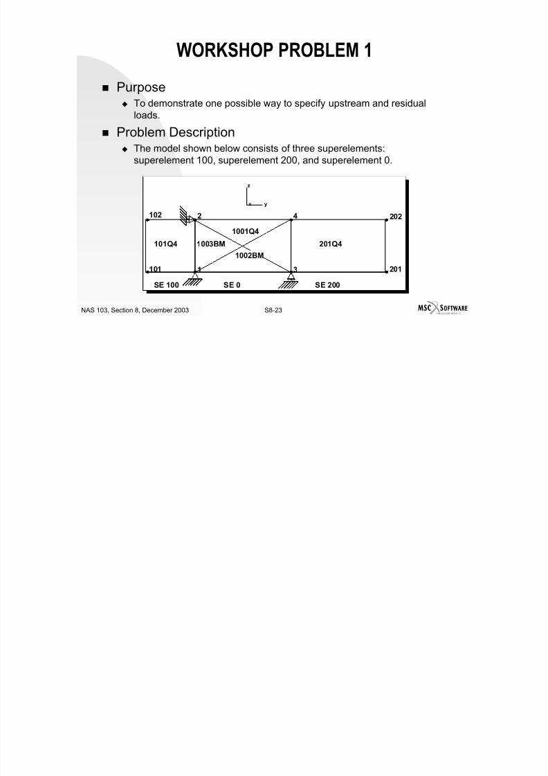
7/21/2019 Nonlinear Analysis Using MSC.nastran
http://slidepdf.com/reader/full/nonlinear-analysis-using-mscnastran 547/783
S8-22NAS 103, Section 8, December 2003
$ (LOADSET) (DAREA) (P-ID) (TID)
LSEQ 1000 101 1LSEQ 1000 102 2LSEQ 1000 103 27
$ Usual LOAD entries
FORCE 1 etc.PLOAD 2 etc.
GRAV 27 etc.
$ CLOAD combines LSEQ loads for upstream superelements$ CID S S1 DAREA S2 DAREA
CLOAD 1001 1.0 386 103 1.0 101CLOAD 1002 1.0 386. 103 1.0 102
CLOAD = CID
WORKSHOP PROBLEM 1
Purpose To demonstrate one possible way to specify upstream and residual
loads.
P bl D i ti
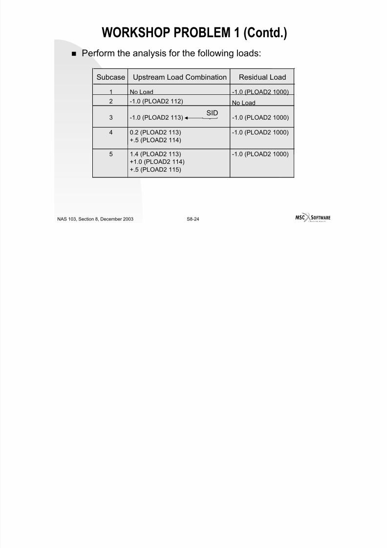
7/21/2019 Nonlinear Analysis Using MSC.nastran
http://slidepdf.com/reader/full/nonlinear-analysis-using-mscnastran 548/783
S8-23NAS 103, Section 8, December 2003
Problem Description The model shown below consists of three superelements:
superelement 100, superelement 200, and superelement 0.
SE 100 SE 0 SE 200
101Q4 1003BM 201Q4
1002BM
102 202
101 201
2 4
31
1001Q4
z
yx
WORKSHOP PROBLEM 1 (Contd.)
Perform the analysis for the following loads:
Subcase Upstream Load Combination Residual Load
1 No Load 1 0 (PLOAD2 1000)
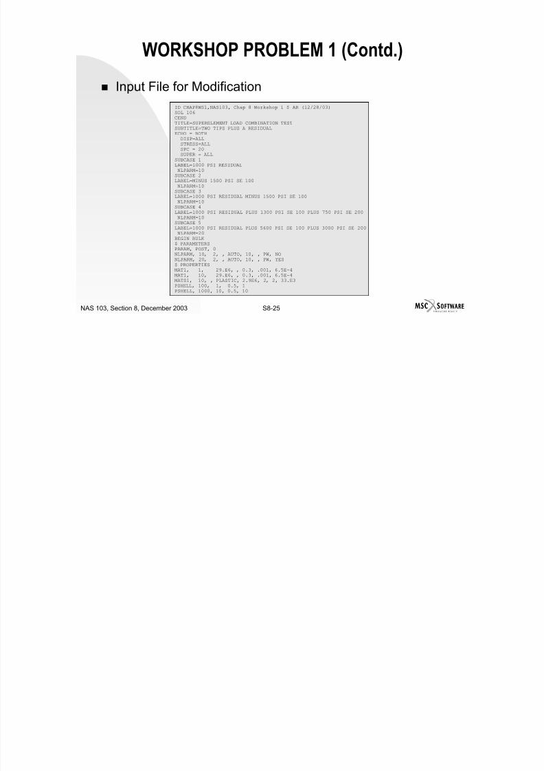
7/21/2019 Nonlinear Analysis Using MSC.nastran
http://slidepdf.com/reader/full/nonlinear-analysis-using-mscnastran 549/783
S8-24NAS 103, Section 8, December 2003
1 No Load -1.0 (PLOAD2 1000)
2 -1.0 (PLOAD2 112) No Load
3 -1.0 (PLOAD2 113) -1.0 (PLOAD2 1000)
4 0.2 (PLOAD2 113)
+.5 (PLOAD2 114)
-1.0 (PLOAD2 1000)
5 1.4 (PLOAD2 113)+1.0 (PLOAD2 114)+.5 (PLOAD2 115)
-1.0 (PLOAD2 1000)
SID
WORKSHOP PROBLEM 1 (Contd.)
Input File for ModificationID CHAP8WS1,NAS103, Chap 8 Workshop 1 $ AR (12/28/03)SOL 106CENDTITLE=SUPERELEMENT LOAD COMBINATION TESTSUBTITLE=TWO TIPS PLUS A RESIDUAL
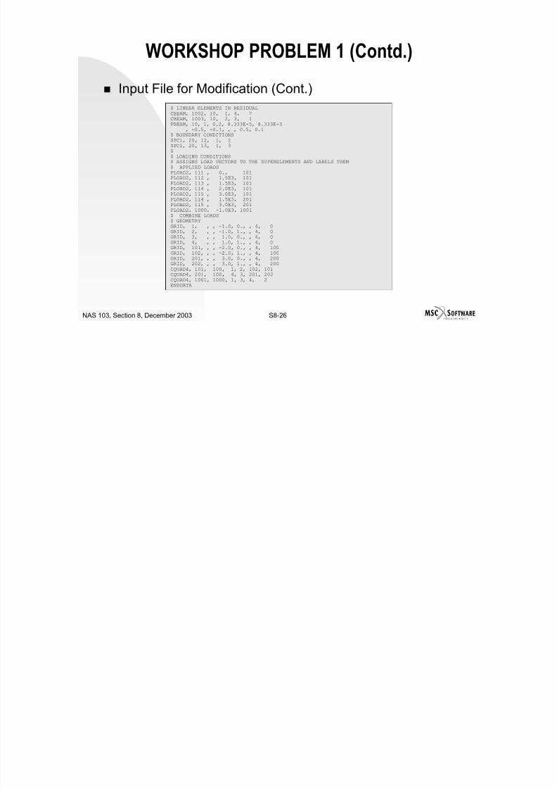
7/21/2019 Nonlinear Analysis Using MSC.nastran
http://slidepdf.com/reader/full/nonlinear-analysis-using-mscnastran 550/783
S8-25NAS 103, Section 8, December 2003
SUBTITLE TWO TIPS PLUS A RESIDUALECHO = BOTH
DISP=ALLSTRESS=ALLSPC = 20SUPER = ALL
SUBCASE 1LABEL=1000 PSI RESIDUALNLPARM=10SUBCASE 2LABEL=MINUS 1500 PSI SE 100NLPARM=10SUBCASE 3
LABEL=1000 PSI RESIDUAL MINUS 1500 PSI SE 100NLPARM=10SUBCASE 4LABEL=1000 PSI RESIDUAL PLUS 1300 PSI SE 100 PLUS 750 PSI SE 200NLPARM=10SUBCASE 5LABEL=1000 PSI RESIDUAL PLUS 5600 PSI SE 100 PLUS 3000 PSI SE 200NLPARM=20BEGIN BULK$ PARAMETERSPARAM, POST, 0
NLPARM, 10, 2, , AUTO, 10, , PW, NONLPARM, 20, 2, , AUTO, 10, , PW, YES$ PROPERTIESMAT1, 1, 29.E6, , 0.3, .001, 6.5E-4MAT1, 10, 29.E6, , 0.3, .001, 6.5E-4MATS1, 10, , PLASTIC, 2.9E6, 2, 2, 33.E3PSHELL, 100, 1, 0.5, 1PSHELL, 1000, 10, 0.5, 10
WORKSHOP PROBLEM 1 (Contd.)
Input File for Modification (Cont.)$ LINEAR ELEMENTS IN RESIDUALCBEAM, 1002, 10, 1, 4, 2CBEAM, 1003, 10, 2, 3, 1PBEAM, 10, 1, 0.2, 8.333E-5, 8.333E-3
, -0.5, -0.1, , , 0.5, 0.1

7/21/2019 Nonlinear Analysis Using MSC.nastran
http://slidepdf.com/reader/full/nonlinear-analysis-using-mscnastran 551/783
S8-26NAS 103, Section 8, December 2003
$ BOUNDARY CONDITIONS
SPC1, 20, 12, 1, 2SPC1, 20, 13, 1, 3$$ LOADING CONDITIONS$ ASSIGNS LOAD VECTORS TO THE SUPERELEMENTS AND LABELS THEM$ APPLIED LOADSPLOAD2, 111 , 0., 101PLOAD2, 112 , 1.5E3, 101PLOAD2, 113 , 1.5E3, 101PLOAD2, 114 , 2.0E3, 101PLOAD2, 115 , 3.0E3, 101PLOAD2, 114 , 1.5E3, 201PLOAD2, 115 , 3.0E3, 201PLOAD2, 1000, -1.0E3, 1001$ COMBINE LOADS$ GEOMETRYGRID, 1, , , -1.0, 0., , 4, 0GRID, 2, , , -1.0, 1., , 4, 0GRID, 3, , , 1.0, 0., , 4, 0GRID, 4, , , 1.0, 1., , 4, 0GRID, 101, , , -2.0, 0., , 4, 100GRID, 102, , , -2.0, 1., , 4, 100GRID, 201, , , 3.0, 0., , 4, 200
GRID, 202, , , 3.0, 1., , 4, 200CQUAD4, 101, 100, 1, 2, 102, 101CQUAD4, 201, 100, 4, 3, 201, 202CQUAD4, 1001, 1000, 1, 3, 4, 2ENDDATA
WORKSHOP PROBLEM 1 (Contd.)
Hints Bulk Data changes:
Define a dummy load PLOAD2, 111 for superelement 100.
Define CLOADs 1010, 1020, 1030, 1040, and 1050 to apply upstream loads

7/21/2019 Nonlinear Analysis Using MSC.nastran
http://slidepdf.com/reader/full/nonlinear-analysis-using-mscnastran 552/783
S8-27NAS 103, Section 8, December 2003
Define CLOADs 1010, 1020, 1030, 1040, and 1050 to apply upstream loads
in subcases 1, 2, 3, 4, and 5, respectively. Define LOAD 10 to apply residual load.
Define LSEQ,100 entries to select PLOAD2 entries with ID = 111 through115.
Case Control changes: Define SUPER = ALL above subcase level. Define LOADSET = 100 above subcase level.
Select LOAD and CLOAD entries for each subcase.
SOLUTION FOR WORKSHOP PROBLEM 1
ID CHAP8WS1s,NAS103, Chap 8 Workshop 1 $ AR (12/28/03)SOL 106CENDTITLE=SUPERELEMENT LOAD COMBINATION TESTSUBTITLE=TWO TIPS PLUS A RESIDUALECHO = BOTHDISP=ALLSTRESS=ALLSPC = 20LOADSET = 100 $ REFERING TO LSEQ FOR UPSTREAM LOADSSUPER = ALL
SUBCASE 1

7/21/2019 Nonlinear Analysis Using MSC.nastran
http://slidepdf.com/reader/full/nonlinear-analysis-using-mscnastran 553/783
S8-28NAS 103, Section 8, December 2003
SUBCASE 1LABEL=1000 PSI RESIDUAL
NLPARM=10LOAD = 10CLOAD = 1010SUBCASE 2LABEL=MINUS 1500 PSI SE 100NLPARM=10CLOAD = 1020SUBCASE 3LABEL=1000 PSI RESIDUAL MINUS 1500 PSI SE 100NLPARM=10LOAD = 10CLOAD = 1030SUBCASE 4
LABEL=1000 PSI RESIDUAL PLUS 1300 PSI SE 100 PLUS 750 PSI SE 200NLPARM=10LOAD = 10CLOAD = 1040SUBCASE 5LABEL=1000 PSI RESIDUAL PLUS 5600 PSI SE 100 PLUS 3000 PSI SE 200NLPARM=20LOAD = 10CLOAD = 1050BEGIN BULK$ PARAMETERSPARAM, POST, 0NLPARM, 10, 2, , AUTO, 10, , PW, NO
NLPARM, 20, 2, , AUTO, 10, , PW, YES$ PROPERTIESMAT1, 1, 29.E6, , 0.3, .001, 6.5E-4MAT1, 10, 29.E6, , 0.3, .001, 6.5E-4MATS1, 10, , PLASTIC, 2.9E6, 2, 2, 33.E3PSHELL, 100, 1, 0.5, 1PSHELL, 1000, 10, 0.5, 10
SOLUTION FOR WORKSHOP PROBLEM 1(Contd.)
$ LINEAR ELEMENTS IN RESIDUALCBEAM, 1002, 10, 1, 4, 2CBEAM, 1003, 10, 2, 3, 1PBEAM, 10, 1, 0.2, 8.333E-5, 8.333E-3
, -0.5, -0.1, , , 0.5, 0.1$ BOUNDARY CONDITIONSSPC1, 20, 12, 1, 2SPC1, 20, 13, 1, 3$ LOADING CONDITIONSLSEQ, 100, 11, 111LSEQ, 100, 12, 112LSEQ 100 13 113

7/21/2019 Nonlinear Analysis Using MSC.nastran
http://slidepdf.com/reader/full/nonlinear-analysis-using-mscnastran 554/783
S8-29NAS 103, Section 8, December 2003
LSEQ, 100, 13, 113
LSEQ, 100, 14, 114LSEQ, 100, 15, 115$ ASSIGNS LOAD VECTORS TO THE SUPERELEMENTS AND LABELS THEM$ APPLIED LOADSPLOAD2, 111 , 0., 101PLOAD2, 112 , 1.5E3, 101PLOAD2, 113 , 1.5E3, 101PLOAD2, 114 , 2.0E3, 101PLOAD2, 115 , 3.0E3, 101PLOAD2, 114 , 1.5E3, 201PLOAD2, 115 , 3.0E3, 201PLOAD2, 1000, -1.0E3, 1001$ COMBINE LOADSLOAD, 10, 1.0, -1.0, 1000CLOAD, 1010, 1.0, -1.0, 11CLOAD, 1020, 1.0, -1.0, 12CLOAD, 1030, 1.0, -1.0, 13CLOAD, 1040, 1.0, 0.2, 13, 0.5, 14CLOAD, 1050, 1.0, 1.4, 13, 1.0, 14, 0.5, 15$ GEOMETRYGRID, 1, , , -1.0, 0., , 4, 0GRID, 2, , , -1.0, 1., , 4, 0GRID, 3, , , 1.0, 0., , 4, 0GRID, 4, , , 1.0, 1., , 4, 0GRID, 101, , , -2.0, 0., , 4, 100GRID, 102, , , -2.0, 1., , 4, 100GRID, 201, , , 3.0, 0., , 4, 200
GRID, 202, , , 3.0, 1., , 4, 200CQUAD4, 101, 100, 1, 2, 102, 101CQUAD4, 201, 100, 4, 3, 201, 202CQUAD4, 1001, 1000, 1, 3, 4, 2ENDDATA

7/21/2019 Nonlinear Analysis Using MSC.nastran
http://slidepdf.com/reader/full/nonlinear-analysis-using-mscnastran 555/783
S8-30NAS 103, Section 8, December 2003

7/21/2019 Nonlinear Analysis Using MSC.nastran
http://slidepdf.com/reader/full/nonlinear-analysis-using-mscnastran 556/783
S9-1NAS 103, Section 9, December 2003
SECTION 9
SPECIAL TOPICS
7/21/2019 Nonlinear Analysis Using MSC.nastran
http://slidepdf.com/reader/full/nonlinear-analysis-using-mscnastran 557/783
S9-2NAS 103, Section 9, December 2003
TABLE OF CONTENTS
PageSpecial Topics 9-5Normal Modes of Deformed Structure 9-6Normal Modes of Prestressed Structure 9-7Normal Modes With Differential Stiffness 9-8
7/21/2019 Nonlinear Analysis Using MSC.nastran
http://slidepdf.com/reader/full/nonlinear-analysis-using-mscnastran 558/783
S9-3NAS 103, Section 9, December 2003
Example Problem 1 –Modes of Preloaded Structure 9-9Input File For Problem 1A – Modes Without Preload 9-11Partial Output File For Problem #1A Modes Without Preload 9-12Input File: Problem #1B – Modes With Preload Using SOL 106 9-13Partial Output File For Problem #1B – Modes With Preload Using
SOL 106 9-14Input File: Problem #1C – Modes With Preload Using SOL 103 9-15Partial Output File For Problem #1C – Modes With Preload Using
SOL 103 9-16
Composite Elements 9-17Features Of Nonlinear Composite Beam 9-18Input Data Entry PBCOMP Beam Property Alternate From For
PBEAM 9-19
TABLE OF CONTENTSPage
Beam Cross-Sectional Area Lumping Scheme For VariousSections 9-21
Smeared Cross-Sectional Properties (I1,I2,I12 Ignored on ParentEntry) 9-23
Features Of Composite Plates 9-25

7/21/2019 Nonlinear Analysis Using MSC.nastran
http://slidepdf.com/reader/full/nonlinear-analysis-using-mscnastran 559/783
S9-4NAS 103, Section 9, December 2003
Laminate And Ply Orientation (PCOMP) 9-262-D Orthotropic Material 9-27Composite Material Specification 9-28Composite Element Specification 9-30
PCOMP – Mat Relationship 9-33 Anisotropic Material In Mat2 9-34Example Problem 2: Composite Cantilever Beam 9-36Failure Theory For Composites 9-40Output For Composite Element 9-42
Smeared Material Properties In PSHELL And MAT2 9-43Layer Stresses In Composite Elements 9-44Failure Index Table 9-45
SPECIAL TOPICS
Nonlinear modal analysis Composite analysis
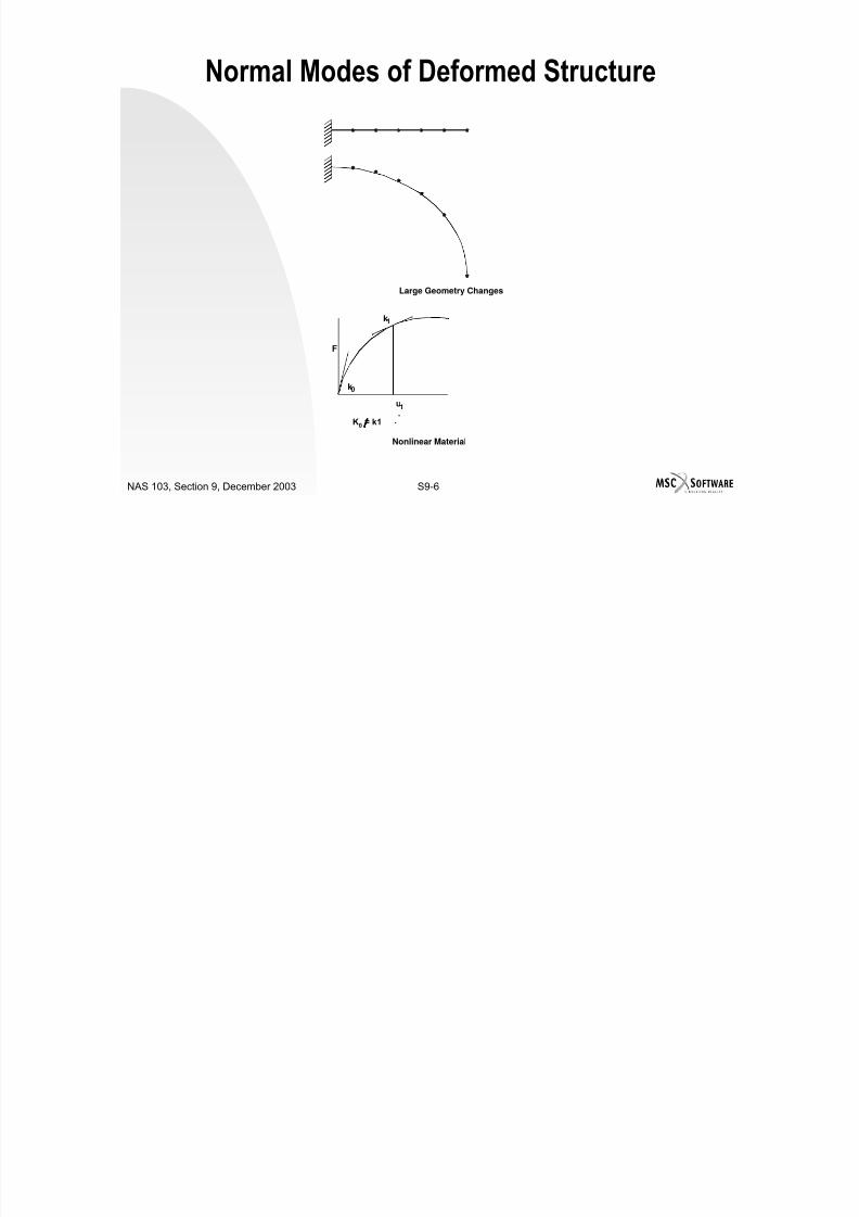
7/21/2019 Nonlinear Analysis Using MSC.nastran
http://slidepdf.com/reader/full/nonlinear-analysis-using-mscnastran 560/783
S9-5NAS 103, Section 9, December 2003
Normal Modes of Deformed Structure

7/21/2019 Nonlinear Analysis Using MSC.nastran
http://slidepdf.com/reader/full/nonlinear-analysis-using-mscnastran 561/783
S9-6NAS 103, Section 9, December 2003
Large Geometry Changes
u1
Nonlinear Material
k1
F
k0
K0 = k1
Normal Modes of Prestressed Structure
Procedures for obtaining frequencies of a preloadedstructure.
Method 1 (Nonlinear Solution for Preload)

7/21/2019 Nonlinear Analysis Using MSC.nastran
http://slidepdf.com/reader/full/nonlinear-analysis-using-mscnastran 562/783
S9-7NAS 103, Section 9, December 2003
Use SOL 106. Include linear or nonlinear material properties as required by modeling.
If material is linear, then only linear material properties are referenced.
Include PARAM,LGDISP,1 in the Bulk Data Section.
Only the residual structure (SEID=0) may contain nonlinear elements. All upstream superelements must be linear.
A METHOD = X Case Control Command in subcase calls out theappropriate EIGRL entry.
Include PARAM,NMLOOP,Y where Y is the loopid that you want to
calculate the normal modes at.
Normal Modes WithDifferential Stiffness (Cont.)
Procedures for obtaining frequencies of a preloadedstructure.
Method 2 (Linear Solution for Preload)

7/21/2019 Nonlinear Analysis Using MSC.nastran
http://slidepdf.com/reader/full/nonlinear-analysis-using-mscnastran 563/783
S9-8NAS 103, Section 9, December 2003
Use SOL 103. Material must be linear.
Two subcases are required.
The first subcase is a static subcase calling out the preload. The second subcase calculates the modes with a METHOD = X
case control command, where X is the appropriate EIGRL ID.
The second subcase must also contain a STATSUB = Y command,where Y is subcase ID of the first subcase.
EXAMPLE PROBLEM 1 -Modes of PreloadedStructure
Consider the simply supported beam as shown below.Calculate the first bending frequency: Case A: Without preload
Case B: With preload using SOL106
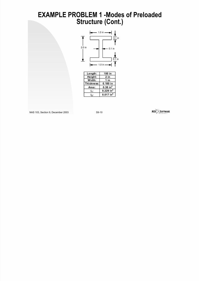
7/21/2019 Nonlinear Analysis Using MSC.nastran
http://slidepdf.com/reader/full/nonlinear-analysis-using-mscnastran 564/783
S9-9NAS 103, Section 9, December 2003
Case C: With preload using SOL 103
P
EXAMPLE PROBLEM 1 -Modes of PreloadedStructure (Cont.)
0.1 in
0.1 in
1.0 in
2.0 in
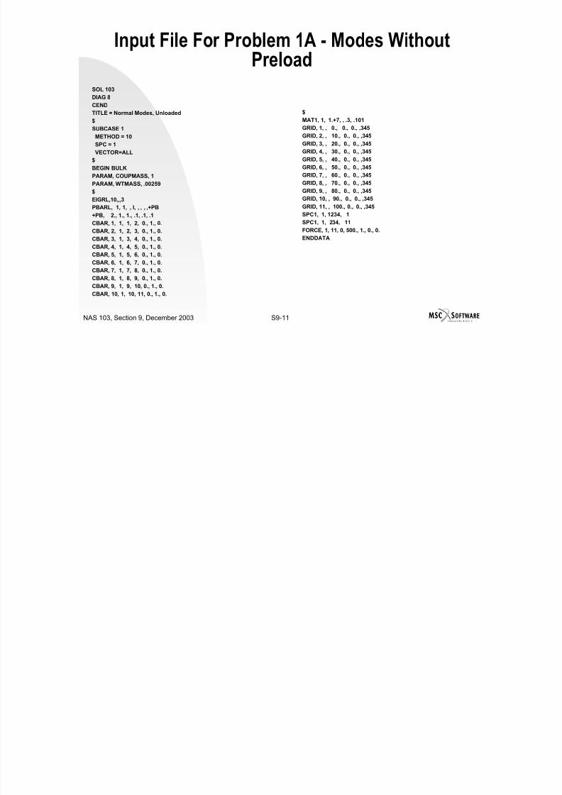
7/21/2019 Nonlinear Analysis Using MSC.nastran
http://slidepdf.com/reader/full/nonlinear-analysis-using-mscnastran 565/783
S9-10NAS 103, Section 9, December 2003
0.1 in
1.0 in
Length: 100 inHeight: 2 in
Width: 1 in
Thickness: 0.100 in
Area: 0.38 in2
I1: 0.229 in4
I2: 0.017 in4
Input File For Problem 1A - Modes WithoutPreload
SOL 103
DIAG 8
CEND
TITLE = Normal Modes, Unloaded
$
SUBCASE 1
METHOD = 10
SPC 1
$
MAT1, 1, 1.+7, , .3, .101
GRID, 1, , 0., 0., 0., ,345
GRID, 2, , 10., 0., 0., ,345
GRID 3 20 0 0 345

7/21/2019 Nonlinear Analysis Using MSC.nastran
http://slidepdf.com/reader/full/nonlinear-analysis-using-mscnastran 566/783
S9-11NAS 103, Section 9, December 2003
SPC = 1VECTOR=ALL
$
BEGIN BULK
PARAM, COUPMASS, 1
PARAM, WTMASS, .00259
$
EIGRL,10,,,3
PBARL, 1, 1, , I, , , , ,+PB+PB, 2., 1., 1., .1, .1, .1
CBAR, 1, 1, 1, 2, 0., 1., 0.
CBAR, 2, 1, 2, 3, 0., 1., 0.
CBAR, 3, 1, 3, 4, 0., 1., 0.
CBAR, 4, 1, 4, 5, 0., 1., 0.
CBAR, 5, 1, 5, 6, 0., 1., 0.
CBAR, 6, 1, 6, 7, 0., 1., 0.
CBAR, 7, 1, 7, 8, 0., 1., 0.
CBAR, 8, 1, 8, 9, 0., 1., 0.
CBAR, 9, 1, 9, 10, 0., 1., 0.
CBAR, 10, 1, 10, 11, 0., 1., 0.
GRID, 3, , 20., 0., 0., ,345GRID, 4, , 30., 0., 0., ,345
GRID, 5, , 40., 0., 0., ,345
GRID, 6, , 50., 0., 0., ,345
GRID, 7, , 60., 0., 0., ,345
GRID, 8, , 70., 0., 0., ,345
GRID, 9, , 80., 0., 0., ,345
GRID, 10, , 90., 0., 0., ,345
GRID, 11, , 100., 0., 0., ,345SPC1, 1, 1234, 1
SPC1, 1, 234, 11
FORCE, 1, 11, 0, 500., 1., 0., 0.
ENDDATA
Partial Output File For Problem #1A ModesWithout Preload
0
E I G E N V A L U E A N A L Y S I S S U M M A R Y (READ MODULE)
BLOCK SIZE USED ...................... 7
NUMBER OF DECOMPOSITIONS ............. 2
NUMBER OF ROOTS FOUND ................ 3

7/21/2019 Nonlinear Analysis Using MSC.nastran
http://slidepdf.com/reader/full/nonlinear-analysis-using-mscnastran 567/783
S9-12NAS 103, Section 9, December 2003
NUMBER OF SOLVES REQUIRED ............ 4
1 NORMAL MODES EXAMPLE APRIL 8, 1998 MSC.Nastran 4/ 6/98 PAGE 5
0 SUBCASE 1
R E A L E I G E N V A L U E S
MODE EXTRACTION EIGENVALUE RADIANS CYCLES GENERALIZED GENERALIZED
NO. ORDER MASS STIFFNESS
1 1 2.239398E+04 1.496462E+02 2.381693E+01 1.000000E+00 2.239398E+04
2 2 3.549898E+05 5.958102E+02 9.482614E+01 1.000000E+00 3.549898E+053 3 1.771818E+06 1.331096E+03 2.118506E+02 1.000000E+00 1.771818E+06
Input File: Problem #1B - Modes With Preload Using SOL 106
SOL 106
TIME 600CEND
TITLE = Normal Modes, Prestressed (nonlinear)
METHOD = 10
SUBCASE 1
NLPARM = 1
SPC = 1
LOAD = 1
DISPLACEMENT=ALL
CBAR, 6, 1, 6, 7, 0., 1., 0.
CBAR, 7, 1, 7, 8, 0., 1., 0.
CBAR, 8, 1, 8, 9, 0., 1., 0.
CBAR, 9, 1, 9, 10, 0., 1., 0.
CBAR, 10, 1, 10, 11, 0., 1., 0.
$
MAT1 1 1 +7 3 101
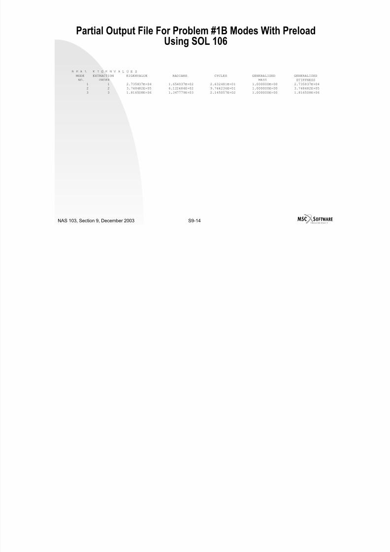
7/21/2019 Nonlinear Analysis Using MSC.nastran
http://slidepdf.com/reader/full/nonlinear-analysis-using-mscnastran 568/783
S9-13NAS 103, Section 9, December 2003
DISPLACEMENT=ALL$
BEGIN BULK
PARAM, COUPMASS, 1
PARAM, WTMASS, .00259
$
PARAM, LGDISP, 1
NLPARM, 1, 5, , AUTO, 5, 25, PW, NO
+NLP, .001, 1.-7
PARAM,NMLOOP,5
$
EIGRL,10,,,3
PBARL, 1, 1, , I, , , , ,+PB
+PB, 2., 1., 1., .1, .1, .1
CBAR, 1, 1, 1, 2, 0., 1., 0.
CBAR, 2, 1, 2, 3, 0., 1., 0.CBAR, 3, 1, 3, 4, 0., 1., 0.
CBAR, 4, 1, 4, 5, 0., 1., 0.
CBAR, 5, 1, 5, 6, 0., 1., 0.
MAT1, 1, 1.+7, , .3, .101
GRID, 1, , 0., 0., 0., ,345
GRID, 2, , 10., 0., 0., ,345
GRID, 3, , 20., 0., 0., ,345
GRID, 4, , 30., 0., 0., ,345
GRID, 5, , 40., 0., 0., ,345
GRID, 6, , 50., 0., 0., ,345
GRID, 7, , 60., 0., 0., ,345GRID, 8, , 70., 0., 0., ,345
GRID, 9, , 80., 0., 0., ,345
GRID, 10, , 90., 0., 0., ,345
GRID, 11, , 100., 0., 0., ,345
SPC1, 1, 1234, 1
SPC1, 1, 234, 11
FORCE, 1, 11, 0, 500., 1., 0., 0.
ENDDATA
Partial Output File For Problem #1B Modes With PreloadUsing SOL 106
R E A L E I G E N V A L U E S
MODE EXTRACTION EIGENVALUE RADIANS CYCLES GENERALIZED GENERALIZED
NO. ORDER MASS STIFFNESS
1 1 2.735837E+04 1.654037E+02 2.632481E+01 1.000000E+00 2.735837E+04
2 2 3.748482E+05 6.122484E+02 9.744236E+01 1.000000E+00 3.748482E+05
3 3 1.816508E+06 1.347779E+03 2.145057E+02 1.000000E+00 1.816508E+06
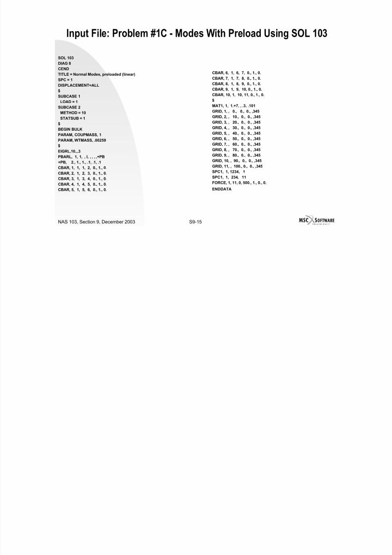
7/21/2019 Nonlinear Analysis Using MSC.nastran
http://slidepdf.com/reader/full/nonlinear-analysis-using-mscnastran 569/783
S9-14NAS 103, Section 9, December 2003
Input File: Problem #1C - Modes With Preload Using SOL 103
SOL 103
DIAG 8
CEND
TITLE = Normal Modes, preloaded (linear)
SPC = 1
DISPLACEMENT=ALL
$
SUBCASE 1
LOAD = 1
CBAR, 6, 1, 6, 7, 0., 1., 0.
CBAR, 7, 1, 7, 8, 0., 1., 0.
CBAR, 8, 1, 8, 9, 0., 1., 0.
CBAR, 9, 1, 9, 10, 0., 1., 0.
CBAR, 10, 1, 10, 11, 0., 1., 0.
$
MAT1 1 1 +7 3 101

7/21/2019 Nonlinear Analysis Using MSC.nastran
http://slidepdf.com/reader/full/nonlinear-analysis-using-mscnastran 570/783
S9-15NAS 103, Section 9, December 2003
LOAD 1SUBCASE 2
METHOD = 10
STATSUB = 1
$
BEGIN BULK
PARAM, COUPMASS, 1
PARAM, WTMASS, .00259
$EIGRL,10,,,3
PBARL, 1, 1, , I, , , , ,+PB
+PB, 2., 1., 1., .1, .1, .1
CBAR, 1, 1, 1, 2, 0., 1., 0.
CBAR, 2, 1, 2, 3, 0., 1., 0.
CBAR, 3, 1, 3, 4, 0., 1., 0.
CBAR, 4, 1, 4, 5, 0., 1., 0.
CBAR, 5, 1, 5, 6, 0., 1., 0.
MAT1, 1, 1.+7, , .3, .101
GRID, 1, , 0., 0., 0., ,345
GRID, 2, , 10., 0., 0., ,345
GRID, 3, , 20., 0., 0., ,345
GRID, 4, , 30., 0., 0., ,345
GRID, 5, , 40., 0., 0., ,345
GRID, 6, , 50., 0., 0., ,345
GRID, 7, , 60., 0., 0., ,345GRID, 8, , 70., 0., 0., ,345
GRID, 9, , 80., 0., 0., ,345
GRID, 10, , 90., 0., 0., ,345
GRID, 11, , 100., 0., 0., ,345
SPC1, 1, 1234, 1
SPC1, 1, 234, 11
FORCE, 1, 11, 0, 500., 1., 0., 0.
ENDDATA
Partial Output File For Problem #1C Modes With PreloadUsing SOL 103
1 NORMAL MODES WITH DIFFERENTIAL STIFFNESS APRIL 9, 1998 MSC.Nastran 4/ 6/98
PAGE 9
0 SUBCASE 2
R E A L E I G E N V A L U E S
MODE EXTRACTION EIGENVALUE RADIANS CYCLES GENERALIZED GENERALIZED
NO. ORDER MASS STIFFNESS1 1 2 735837E+04 1 654037E+02 2 632481E+01 1 000000E+00 2 735837E+04

7/21/2019 Nonlinear Analysis Using MSC.nastran
http://slidepdf.com/reader/full/nonlinear-analysis-using-mscnastran 571/783
S9-16NAS 103, Section 9, December 2003
1 1 2.735837E+04 1.654037E+02 2.632481E+01 1.000000E+00 2.735837E+04
2 2 3.748482E+05 6.122484E+02 9.744236E+01 1.000000E+00 3.748482E+05
3 3 1.816508E+06 1.347779E+03 2.145057E+02 1.000000E+00 1.816508E+06
COMPOSITE ELEMENTS
Beam with PBCOMP QUAD4 and TRIA3 with PCOMP and MAT8

7/21/2019 Nonlinear Analysis Using MSC.nastran
http://slidepdf.com/reader/full/nonlinear-analysis-using-mscnastran 572/783
S9-17NAS 103, Section 9, December 2003
FEATURES OF NONLINEAR COMPOSITEBEAM
BEAM properties in PBCOMP. May be used for geometric and material nonlinear
problems.
Distribution of lumped areas of the BEAM cross section
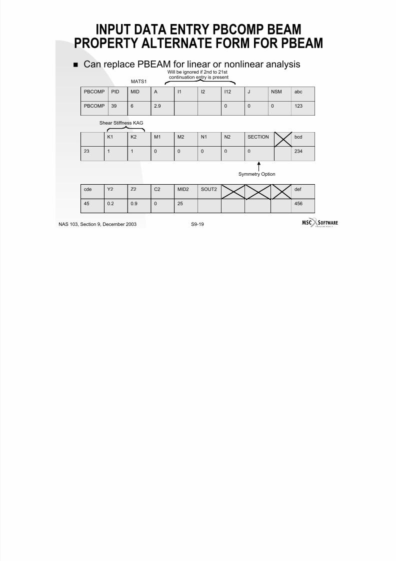
7/21/2019 Nonlinear Analysis Using MSC.nastran
http://slidepdf.com/reader/full/nonlinear-analysis-using-mscnastran 573/783
S9-18NAS 103, Section 9, December 2003
Distribution of lumped areas of the BEAM cross sectionin arbitrary configuration.
Different material for each of the lumped areas allowed.
Maximum of 20 lumped areas may be input. The BEAM is assumed to be uniform (non-tapered).
Warping effects are ignored.
INPUT DATA ENTRY PBCOMP BEAMPROPERTY ALTERNATE FORM FOR PBEAM
Can replace PBEAM for linear or nonlinear analysisWill be ignored if 2nd to 21stcontinuation entry is present
MATS1
1230002.9639PBCOMP
abcNSMJI12I2I1 AMIDPIDPBCOMP

7/21/2019 Nonlinear Analysis Using MSC.nastran
http://slidepdf.com/reader/full/nonlinear-analysis-using-mscnastran 574/783
S9-19NAS 103, Section 9, December 2003
234000001123
bcdSECTIONN2N1M2M1K2K1
Shear Stiffness KAG
Symmetry Option
4562500.90.245
def SOUT2MID2C2Z2Y2cde
INPUT DATA ENTRY PBCOMP BEAMPROPERTY ALTERNATE FORM FOR PBEAM
345NO1801.2-0.534
cdeSOUT1MID1C1Z1Y1bcd
If blank, use parent entry.
For heat transfer, use only MAT4 and/or MAT 5.
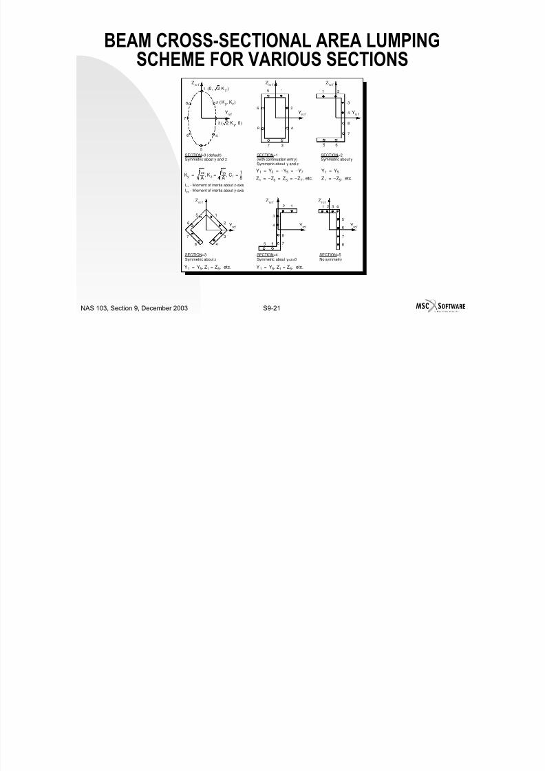
7/21/2019 Nonlinear Analysis Using MSC.nastran
http://slidepdf.com/reader/full/nonlinear-analysis-using-mscnastran 575/783
S9-20NAS 103, Section 9, December 2003
Continue 18 more times for a total of 21 continuationentries.
Need E, ν or E, G on MAT1 entry for parent entry.
p y
BEAM CROSS-SECTIONAL AREA LUMPINGSCHEME FOR VARIOUS SECTIONS
Zre f 1
2
3
4
5
6
7
8
Yref
0 2 K z,( )
Ky Kz,( )
2 K y 0,( )
Zre f Zre f
Yre f Yre f
1
2
3
4
5
6
8
7
1 2
3
4
5 6
8
7

7/21/2019 Nonlinear Analysis Using MSC.nastran
http://slidepdf.com/reader/full/nonlinear-analysis-using-mscnastran 576/783
S9-21NAS 103, Section 9, December 2003
SECTION=0 ( default)Symmetric about y and z
SECTION=1(with continuation entry)Symmetric about y and z
SECTION=2Symmetric about y
SECTION=3
Symmetric about z
SECTION=4
Symmetric about y=z=0
SECTION=5
No symmetry
Izz - Moment of inertia about z-axis
Iyy - Moment of inertia about y-axis
Ky
Izz
A------ Kz
Iyy
A------ C1
1
8---=,=,=
Y1 Y3 Y5– Y– 7= = =
Z1 Z3– Z5 Z7 etc.,–= = =
Y1 Y5=
Z1 Z– 5 etc.,=
Zre f Zre f Zr ef
Yref Yref Yre f
1
2
3
4
5
6
7
8
12
3
4
8
75 6
1 2 3 4
5
6
7
8
Y1 Y5 Z1 Z5 etc.,=,= Y1 Y5 Z1 Z5 etc.,=,=
BEAM CROSS-SECTIONAL AREA LUMPINGSCHEME FOR VARIOUS SECTIONS
Notes: 1. Integration points (lumped areas) are numbered 1-8, to be referenced
by stress output request (SO field).
2. User-specified points are denoted by •, and the program default
points are denoted by ¤.

7/21/2019 Nonlinear Analysis Using MSC.nastran
http://slidepdf.com/reader/full/nonlinear-analysis-using-mscnastran 577/783
S9-22NAS 103, Section 9, December 2003
points are denoted by . 3. Underlined words refer to fields on the PBCOMP entry (Section 5 of
the MSC/NASTRAN Quick Reference Guide).
4. Use 1/2 areas on the symmetric boundary.
SMEARED CROSS-SECTIONAL PROPERTIES(I1,I2,I12 Ignored on Parent Entry)
Offset of neutral axis
yNA
yi C
i E
i
i 1=
n
∑
Ci E i
n
∑
-------------------------------=
PBCOMP Field 4 of each continuation
SEAL2 Field 1
MAT1
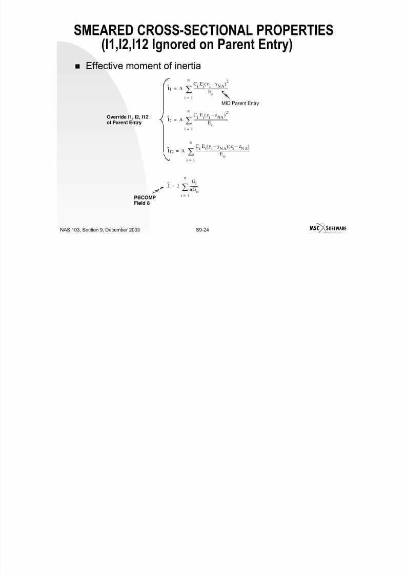
7/21/2019 Nonlinear Analysis Using MSC.nastran
http://slidepdf.com/reader/full/nonlinear-analysis-using-mscnastran 578/783
S9-23NAS 103, Section 9, December 2003
Effective cross-sectional area
i 1=∑ PBCOMP Field 4 of each continuation
line greater than 1.
zNA
zi C
i E
i
i 1=
n
∑
Ci E
i
i 1=
n
∑
------------------------------=
A A= zi
Ci E
iEo
---------------
i 1=
n
∑
PBCOMP Field 4
SMEARED CROSS-SECTIONAL PROPERTIES(I1,I2,I12 Ignored on Parent Entry)
Effective moment of inertia
I1 AC
i E
iy
iy
NA–( )
2
Eo
------------------------------------------
i 1=
n
∑=
MID Parent Entry
C E z z( )2n
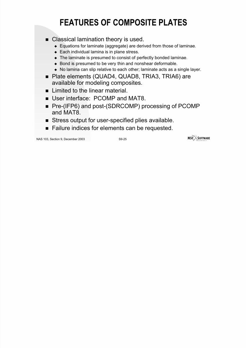
7/21/2019 Nonlinear Analysis Using MSC.nastran
http://slidepdf.com/reader/full/nonlinear-analysis-using-mscnastran 579/783
S9-24NAS 103, Section 9, December 2003
PBCOMPField 8
Override I1, I2, I12of Parent Entry
I2 AC
i E
iz
iz
NA–( )
Eo
------------------------------------------
i 1=
∑=
I12 A
Ci E
iy
iy
NA–( ) z
izNA
–( )
Eo
------------------------------------------------------------------
i 1=
n
∑=
J JG
i
nGo
----------
i 1=
n
∑=
FEATURES OF COMPOSITE PLATES
Classical lamination theory is used. Equations for laminate (aggregate) are derived from those of laminae. Each individual lamina is in plane stress. The laminate is presumed to consist of perfectly bonded laminae.
Bond is presumed to be very thin and nonshear deformable. No lamina can slip relative to each other; laminate acts as a single layer

7/21/2019 Nonlinear Analysis Using MSC.nastran
http://slidepdf.com/reader/full/nonlinear-analysis-using-mscnastran 580/783
S9-25NAS 103, Section 9, December 2003
p y No lamina can slip relative to each other; laminate acts as a single layer.
Plate elements (QUAD4, QUAD8, TRIA3, TRIA6) areavailable for modeling composites.
Limited to the linear material. User interface: PCOMP and MAT8. Pre-(IFP6) and post-(SDRCOMP) processing of PCOMP
and MAT8. Stress output for user-specified plies available. Failure indices for elements can be requested.
LAMINATE AND PLY ORIENTATION (PCOMP)
Z
Y
n

7/21/2019 Nonlinear Analysis Using MSC.nastran
http://slidepdf.com/reader/full/nonlinear-analysis-using-mscnastran 581/783
S9-26NAS 103, Section 9, December 2003
T
θ
X
Y
X
21
12
Z0
Y
2-D ORTHOTROPIC MATERIAL
Orthotropic material in plane stress requires:
Material constants in terms of E1, E2, ν12, AND G12
σ3
0 τ13
0 and τ23
0=,=,=
E1 E1ν21
0

7/21/2019 Nonlinear Analysis Using MSC.nastran
http://slidepdf.com/reader/full/nonlinear-analysis-using-mscnastran 582/783
S9-27NAS 103, Section 9, December 2003
where E2 ν12 = E1 ν21
Transverse shear effects included (G1z, G2z) (Mindlin orReisner plate).
σ1
σ2
τ
12
1
1 ν12ν21–--------------------------
1 21
1 ν12ν21–-------------------------- 0
E2ν
12
1 ν12
ν21
–--------------------------
E2
1 ν12
ν21
–-------------------------- 0
0 0 G12
ε1
ε2
γ
12
=
COMPOSITE MATERIAL SPECIFICATION
SYcYtXcXtTREF A2 A1
00.0561.5+63.+62.+60.31.+630.+6100MAT8
RHOG2zG1zG12n12E2E1MIDMAT8
10987654321

7/21/2019 Nonlinear Analysis Using MSC.nastran
http://slidepdf.com/reader/full/nonlinear-analysis-using-mscnastran 583/783
S9-28NAS 103, Section 9, December 2003
Field Contents
MAT8 Input data for each ply. May be replaced by MAT2
E1, E2 Moduli in principal directions
n12 e2/e1 uniaxial loading in 1-direction
01.+38.+22.+21.5+41.+41551.5-628.-60
1.-30
F12GE
COMPOSITE MATERIAL SPECIFICATION
Field ContentsG12 In-plane shear modulus
G1z, G2z Transverse shear moduli in 1-z and 2-z planes
RHO Mass density
TREF Reference temperature for calculation of thermalloads or a temperature dependent thermal

7/21/2019 Nonlinear Analysis Using MSC.nastran
http://slidepdf.com/reader/full/nonlinear-analysis-using-mscnastran 584/783
S9-29NAS 103, Section 9, December 2003
p pexpansion coefficient
A1, A2 Thermal expansion coefficients in the 1- and 2-directions
Xt, Xc, Yt Tension and compression allowable stresses in 1-and 2- directions
S Allowable stress in plane shear for failure index
GE Structural damping
F12 Interaction term in Tsai-Wu failure theory
Example:
COMPOSITE ELEMENT SPECIFICATION
Etc.SOUT3THETA3T3MID3
SOUT2THETA2T2MID2SOUT1THETA1T1MID1
LAMGETREFFTSBNSMZ0PIDPCOMP10987654321

7/21/2019 Nonlinear Analysis Using MSC.nastran
http://slidepdf.com/reader/full/nonlinear-analysis-using-mscnastran 585/783
S9-30NAS 103, Section 9, December 2003
Example:
Field Contents
PID Property identification number. (0 < Integer < 106)
Z0 Distance from the reference plane to the bottomsurface. See Remark 10. (Real; Default = -1/2 thethickness of the element)
90-45
45YES00.056171
HOFF1000.07.45-0.224181PCOMP
COMPOSITE ELEMENT SPECIFICATION
Field ContentsNSM Nonstructural mass per unit area. (Real)SB Allowable shear stress of the bonding material (allowable
interlaminar shear stress). Required if failure index is desired.(Real > 0.0)
FT Failure theory. The following theories are allowed (Characteror blank. If blank, then no failure calculation will be

7/21/2019 Nonlinear Analysis Using MSC.nastran
http://slidepdf.com/reader/full/nonlinear-analysis-using-mscnastran 586/783
S9-31NAS 103, Section 9, December 2003
o b a b a , t e o a u e ca cu at o beperformed):
“HILL” for the Hill theory“HOFF” for the Hoffman theory
“TSAI” for the Tsai-Wu theory“STRN” for the maximum strain theory
TREF Reference temperature. See Remark 3. (Real).GE Damping coefficient. See Remark 4g. (Real; Default =0.0).
LAM Symmetric lamination option. If LAM = “SYM”, only
COMPOSITE ELEMENT SPECIFICATION
Field ContentsMIDi Material ID of the various plies. The plies are identified by
serially numbering them from 1 at the bottom layer. The MIDsmust refer to MAT1, MAT2, or MAT8 Bulk Data entries. SeeRemark 1. (Integer > 0 or blank except MID1 must be
specified).Ti Thickness of the various plies. See Remark 1. (Real or blank

7/21/2019 Nonlinear Analysis Using MSC.nastran
http://slidepdf.com/reader/full/nonlinear-analysis-using-mscnastran 587/783
S9-32NAS 103, Section 9, December 2003
except T1 must be specified).THETAi Orientation angle of the longitudinal direction of each ply with
the material axis of the element. (If the material angle on the
element connection entry is 0.0, the material axis and side102 of the element coincide). The plies are to be numberedserially starting with 1 at the bottom layer. The bottom layer isdefined as the surface with the largest –Z value in theelement coordinate system. (Real; Default = 0.0).
SOUTi Stress or strain output request. See Remarks 5 and 6.
(Character: “YES” or “NO”; Default = “NO”).
PCOMP - MAT RELATIONSHIP
CQUAD4
PBCOMP
MAT1 MAT3MAT2

7/21/2019 Nonlinear Analysis Using MSC.nastran
http://slidepdf.com/reader/full/nonlinear-analysis-using-mscnastran 588/783
S9-33NAS 103, Section 9, December 2003
EQUIV PSHELL*
MID1MAT2
MID4MAT4
MID3MAT3
MID2MAT2
ANISOTROPIC MATERIAL IN MAT2
+M225.1+36.2+36.2+3100MAT2
RHOG33G23G22G13G12G11MIDMAT210987654321
+M2320.+50.0025006.5-66.5-6+M22
SSSCSTGETREF A12 A2 A1

7/21/2019 Nonlinear Analysis Using MSC.nastran
http://slidepdf.com/reader/full/nonlinear-analysis-using-mscnastran 589/783
S9-34NAS 103, Section 9, December 2003
Field Contents
Gii Material constants
RHO Mass density A1, A2, A12 Thermal expansion coefficients
1003+M29
MCSID
ANISOTROPIC MATERIAL IN MAT2
Field ContentsTREF Reference temperature for the calculation of thermal loads
GE Structural damping
ST, SC, SS Stress limit in tension, compression and shear for
computing margin of safetyMCSID Material coordinate system ID
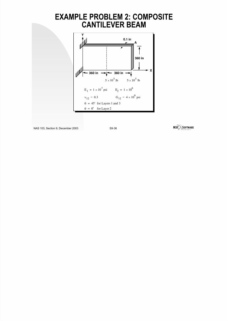
7/21/2019 Nonlinear Analysis Using MSC.nastran
http://slidepdf.com/reader/full/nonlinear-analysis-using-mscnastran 590/783
S9-35NAS 103, Section 9, December 2003
σ1
σ2
τ12
G11 G12 G13
G22 G23
SYM G33
ε1
ε2
γ12
T T0–( )
A1
A2
A12
–=
EXAMPLE PROBLEM 2: COMPOSITECANTILEVER BEAM
Y
A0.1 in
360 in

7/21/2019 Nonlinear Analysis Using MSC.nastran
http://slidepdf.com/reader/full/nonlinear-analysis-using-mscnastran 591/783
S9-36NAS 103, Section 9, December 2003
X360 in360 in
5 105
× lb 5 105 lb×
E1 1 107 psi×= E2 1 10
6×=
ν12 0.3= G12 4 106 psi×=
θ 45o for Layers 1 and 3=
θ 00
for Layer 2=
Input File For Example 2 – CompositeCantilever Beam
ID, chap9ex2b, NAS103, chap 8 Ex 2 (Nonlinear)SOL 106
CEND
TITLE = Cantilever Composite Beam of NAS103 chapter 9
ECHO=SORT
SUBCASE 1
SPC = 1
LOAD = 1
NLPARM = 10
DISPLACEMENT(SORT1,REAL)=ALL
SPCFORCES(SORT1,REAL)=ALL
$ ElementsCQUAD4, 1, 1, 1, 2, 15, 14
CQUAD4, 2, 1, 2, 3, 16, 15
CQUAD4, 3, 1, 3, 4, 17, 16
CQUAD4, 4, 1, 4, 5, 18, 17
CQUAD4, 5, 1, 5, 6, 19, 18
CQUAD4, 6, 1, 6, 7, 20, 19
CQUAD4, 7, 1, 7, 8, 21, 20
CQUAD4, 8, 1, 8, 9, 22, 21
CQUAD4, 9, 1, 9, 10, 23, 22
CQUAD4, 10, 1, 10, 11, 24, 23

7/21/2019 Nonlinear Analysis Using MSC.nastran
http://slidepdf.com/reader/full/nonlinear-analysis-using-mscnastran 592/783
S9-37NAS 103, Section 9, December 2003
SPCFORCES(SORT1,REAL) ALL
STRESS(SORT1,REAL,VONMISES,BILIN)=ALL
BEGIN BULK
PARAM, POST, 0
PARAM, AUTOSPC, YES
PARAM, PRTMAXIM, YES
PARAM, LGDISP, 2
$ NONLINEAR SOLUTION STRATEGY
NLPARM, 10, 1, , AUTO, , , PW, YES, +NLP1
+NLP1, , 1.E-2, 1.E-3
$ Composite Material
PCOMP, 1,
, 1, .02, 45., YES, 1, .06, 0., YES
, 1, .02, 45., YES
CQUAD4, 10, 1, 10, 11, 24, 23
CQUAD4, 11, 1, 11, 12, 25, 24
CQUAD4, 12, 1, 12, 13, 26, 25
….
….
CQUAD4, 61, 1, 66, 67, 80, 79CQUAD4, 62, 1, 67, 68, 81, 80
CQUAD4, 63, 1, 68, 69, 82, 81
CQUAD4, 64, 1, 69, 70, 83, 82
CQUAD4, 65, 1, 70, 71, 84, 83
CQUAD4, 66, 1, 71, 72, 85, 84
CQUAD4, 67, 1, 72, 73, 86, 85
CQUAD4, 68, 1, 73, 74, 87, 86
CQUAD4, 69, 1, 74, 75, 88, 87CQUAD4, 70, 1, 75, 76, 89, 88
CQUAD4, 71, 1, 76, 77, 90, 89
CQUAD4, 72, 1, 77, 78, 91, 90
Input File For Problem 1A - Modes WithoutPreload
$ Material Properties
MAT8, 1, 1.E7, 1.E6, .3, 4.E6
$ Nodes
GRID, 1, , 0., 0., 0.
GRID, 2, , 60., 0., 0.
GRID, 3, , 120., 0., 0.
GRID, 4, , 180., 0., 0.
GRID, 5, , 240., 0., 0.
GRID, 6, , 300., 0., 0.
GRID, 79, , 0., 360., 0.
GRID, 80, , 60., 360., 0.
GRID, 81, , 120., 360., 0.
GRID, 82, , 180., 360., 0.
GRID, 83, , 240., 360., 0.
GRID, 84, , 300., 360., 0.
GRID, 85, , 360., 360., 0.
GRID, 86, , 420., 360., 0.
GRID, 87, , 480., 360., 0.
GRID 88 540 360 0

7/21/2019 Nonlinear Analysis Using MSC.nastran
http://slidepdf.com/reader/full/nonlinear-analysis-using-mscnastran 593/783
S9-38NAS 103, Section 9, December 2003
GRID, 6, , 300., 0., 0.
GRID, 7, , 360., 0., 0.
GRID, 8, , 420., 0., 0.
GRID, 9, , 480., 0., 0.
GRID, 10, , 540., 0., 0.
GRID, 11, , 600., 0., 0.GRID, 12, , 660., 0., 0.
GRID, 13, , 720., 0., 0.
….
….
GRID, 88, , 540., 360., 0.
GRID, 89, , 600., 360., 0.
GRID, 90, , 660., 360., 0.
GRID, 91, , 720., 360., 0.
$
SPC1, 1, 123456, 1, 14, 27, 40, 53, 66, 79
$
FORCE, 1, 7, 0, 5.E5, 0., -1., 0.
FORCE, 1, 13, 0, 5.E5, 0., -1., 0.
$
ENDDATA
EXAMPLE PROBLEM 2: COMPOSITE
CANTILEVER BEAM (Contd.)
Vertical Displacement at Point A
(with a 12X6 Mesh of Quad4)

7/21/2019 Nonlinear Analysis Using MSC.nastran
http://slidepdf.com/reader/full/nonlinear-analysis-using-mscnastran 594/783
S9-39NAS 103, Section 9, December 2003
LAYER THICKNESSES DISPLACEMENT
Linear (SOL 101) Nonlinear (SOL 106)
0.02/0.06/0.02 28.95 28.49
0.03/0.04/0.03 33.48 32.90
0.04/0.02/0.04 41.94 41.08
FAILURE THEORY FOR COMPOSITES
Allowable stresses are direction dependent. Failure envelope is defined in the stress space.
Failure index is a measure whether the stress state in
the worst stressed lamina is within or outside theenvelope.

7/21/2019 Nonlinear Analysis Using MSC.nastran
http://slidepdf.com/reader/full/nonlinear-analysis-using-mscnastran 595/783
S9-40NAS 103, Section 9, December 2003
Inter-laminar shear stress is checked against theallowable bonding stress (Sb).
Failure index for the laminate is the larger of the two.
FAILURE THEORY FOR COMPOSITES
Laminate has failed if the failure index is greater than 1. Failure envelope is defined by:
Hills’s theory (ellipsoidal).
Hoffman’s theory. Accounts for differing tension and compression.
Tensor polynomial theory (Tsai-Wu): closed envelope.
Maximum strain theory.

7/21/2019 Nonlinear Analysis Using MSC.nastran
http://slidepdf.com/reader/full/nonlinear-analysis-using-mscnastran 596/783
S9-41NAS 103, Section 9, December 2003
Maximum strain theory.
OUTPUT FOR COMPOSITE ELEMENT
Smeared material properties for equivalent PSHELL andMAT2 data. Requires ECHO = SORT.
Smeared stresses in linear stress output format. Usualstress output request.
Stresses in individual lamina (including inter-laminarh t ) R i YES SOUT fi ld

7/21/2019 Nonlinear Analysis Using MSC.nastran
http://slidepdf.com/reader/full/nonlinear-analysis-using-mscnastran 597/783
S9-42NAS 103, Section 9, December 2003
shear stresses). Requires YES on SOUT field onPCOMP.
Failure index table Requires ELFORCE and ELSTRESS requests.
Allowable stresses must be provided on MAT8.
SMEARED MATERIAL PROPERTIES INPSHELL AND MAT2
For ECHO = SORTCOMPOSITE ELEMENTS SOL 106 MARCH 15, 1993 MSC/NASTRAN 3/12/93 PAGE 5*** USER INFORMATION MESSAGE 4379, THE USER SUPPLIED PCOMP BULK DATA CARDS ARE REPLACED BY THE FOLLOWING PSHELL AND MAT2CARDS.
PSHELL 100 100000100 2.0000E-01 200000100 1.0000E+00 300000100 1.0000E+00 0.0000E+00-1.0000E-01 1.0000E-01 0
MAT2 100000100 1.4286E+07 4.2857E+06 2.5241E-08 1.4286E+07 1.5806E-09 5.0000E+06 0.0000E+000.0000E+00 0.0000E+00 0.0000E+00 0.0000E+00 0.0000E+00 0.0000E+00 0.0000E+00 0.0000E+00
0MAT2 200000100 1.4286E+07 4.2857E+06 2.0446E-08 1.4286E+07 1.2803E-09 5.0000E+06 0.0000E+00
0.0000E+00 0.0000E+00 0.0000E+00 0.0000E+00 0.0000E+00 0.0000E+00 0.0000E+00 0.0000E+000
MAT2 300000100 4 1667E+06 0 0000E+00 0 0000E+00 4 1667E+06 0 0000E+00 0 0000E+00 0 0000E+00

7/21/2019 Nonlinear Analysis Using MSC.nastran
http://slidepdf.com/reader/full/nonlinear-analysis-using-mscnastran 598/783
S9-43NAS 103, Section 9, December 2003
MAT2 300000100 4.1667E+06 0.0000E+00 0.0000E+00 4.1667E+06 0.0000E+00 0.0000E+00 0.0000E+00
0.0000E+00 0.0000E+00 0.0000E+00 0.0000E+00 0.0000E+00 0.0000E+00 0.0000E+00 0.0000E+000
LAYER STRESSES IN COMPOSITE ELEMENTS
COMPOSITE ELEMENTS SOL 106 MARCH 15, 1993 MSC/NASTRAN 3/12/93 PAGE 103
SUBCASE 1
S T R E S S E S I N L A Y E R E D C O M P O S I T E E L E M E N T S ( Q U A D 4 )ELEMENT PLY STRESSES IN FIBRE AND MATRIX DIRECTIONS INTER-LAMINAR STRESSES PRINCIPAL STRESSES (ZERO SHEAR) MAXID ID NORMAL-1 NORMAL-2 SHEAR-12 SHEAR-1Z SHEAR-2Z ANGLE MAJOR MINOR SHEAR101 1 -4.07141E+05 -1.35714E+06 -1.69456E+02 7.84304E+02 2.02505E-14 -.01 -4.07141E+05 -1.35714E+06 4.75001E+05101 3 4.07141E+05 1.35714E+06 1.69456E+02 5.49630E-12 1.41913E-28 89.99 1.35714E+06 4.07141E+05 4.75001E+05102 1 -4.07139E+05 -1.35714E+06 -8.32131E+02 5.71212E+02 4.69811E-12 -.05 -4.07138E+05 -1.35714E+06 4.75002E+05102 3 4.07139E+05 1.35714E+06 8.32131E+02 4.00298E-12 3.29237E-26 89.95 1.35714E+06 4.07138E+05 4.75002E+05103 1 -4.07137E+05 -1.35714E+06 -1.19496E+03 3.82783E+02 2.43006E-13 -.07 -4.07136E+05 -1.35714E+06 4.75003E+05
103 3 4.07137E+05 1.35714E+06 1.19496E+03 2.68250E-12 1.70295E-27 89.93 1.35714E+06 4.07136E+05 4.75003E+05104 1 -4.07137E+05 -1.35714E+06 -9.55886E+02 2.18618E+02 -8.70770E-13 -.06 -4.07136E+05 -1.35714E+06 4.75003E+05104 3 4.07137E+05 1.35714E+06 9.55886E+02 1.53205E-12 -6.10225E-27 89.94 1.35714E+06 4.07136E+05 4.75003E+05105 1 -4.07136E+05 -1.35714E+06 -4.99785E+02 7.09528E+01 2.78697E-12 -.03 -4.07136E+05 -1.35714E+06 4.75003E+05105 3 4.07136E+05 1.35714E+06 4.99785E+02 4.97228E-13 1.95307E-26 89.97 1.35714E+06 4.07136E+05 4.75003E+05

7/21/2019 Nonlinear Analysis Using MSC.nastran
http://slidepdf.com/reader/full/nonlinear-analysis-using-mscnastran 599/783
S9-44NAS 103, Section 9, December 2003
FAILURE INDEX TABLE
1 COMPOSITE ELEMENTS SOL 106 MARCH 15, 1993 MSC/NASTRAN 3/12/93 PAGE 104
0 SUBCASE 1 $
F A I L U R E I N D I C E S F O R L A Y E R E D C O M P O S I T E E L E M E N T S ( Q U A D 4 )ELEMENT FAILURE PLY FP=FAILURE INDEX FOR PLY FB=FAILURE INDEX FOR BONDING FAILURE INDEX FOR ELEMENT FLAGID THEORY ID (DIRECT STRESSES/STRAINS) (INTER-LAMINAR STRESSES) MAX OF FP,FB FOR ALL PLIES101 HILL 1 582.0204
.78432 .0000
.78433 582.0204
582.0204 ***102 HILL 1 582.0205
.57122 .0000
.57123 582 0206

7/21/2019 Nonlinear Analysis Using MSC.nastran
http://slidepdf.com/reader/full/nonlinear-analysis-using-mscnastran 600/783
S9-45NAS 103, Section 9, December 2003
3 582.0206582.0206 ***
103 HILL 1 582.0208.3828
2 .0000.3828
3 582.0208 582.0208 ***104 HILL 1 582.0205
.21862 .0000
.21863 582.0205
582.0205 ***105 HILL 1 582.0202
.07102 .0000
.07103 582.0203582.0203 ***

7/21/2019 Nonlinear Analysis Using MSC.nastran
http://slidepdf.com/reader/full/nonlinear-analysis-using-mscnastran 601/783
S9-46NAS 103, Section 9, December 2003
SECTION 10

7/21/2019 Nonlinear Analysis Using MSC.nastran
http://slidepdf.com/reader/full/nonlinear-analysis-using-mscnastran 602/783
10-1NAS 103, SOL 600, December 2003
SOL 600

7/21/2019 Nonlinear Analysis Using MSC.nastran
http://slidepdf.com/reader/full/nonlinear-analysis-using-mscnastran 603/783
10-2NAS 103, SOL 600, December 2003
TABLE OF CONTENTS
PageMSC.Nastran Implicit Nonlinear(SOL 600) Analysis 10-7
Overview Of NonLinear Analysis Using MSC.Nastran SOL 600 10-8
MSC.Nastran SOL 600 Overview 10-9
What Is MSC.Nastran SOL 600? 10-10Nonlinear Capabilities In MSC.Nastran 10-11
What Is MSC Marc? 10-12

7/21/2019 Nonlinear Analysis Using MSC.nastran
http://slidepdf.com/reader/full/nonlinear-analysis-using-mscnastran 604/783
10-3NAS 103, SOL 600, December 2003
What Is MSC.Marc? 10 12
What Is MSC.Marc? – Summary 10-15
What Is MSC.Nastran SOL 600 10-16
What Is MSC.Patran? 10-17
MSC.Patran Is A Pre- & Post-Processor 10-19
MSC.Nastran SOL 600 Is Open Architecture 10-20
What Is MSC.Nastran SOL 600? 10-21
Why Should I Use MSC.Nastran SOL 600? 10-22
How Does MSC.Nastran SOL 600 Work? 10-24
TABLE OF CONTENTS
PageFeatures And Capabilities 10-28
Summary of MSC.Nastran SOL 600 Nonlinear Analysis Capabilities 10-29
Non-Linear Capabilities In MSC.Nastrain SOL 600 10-30
Geometric Non-Linearities 10-31Geometric Non-Linearities - Finite Deformation 10-32
Geometric Nonlinearity – Follower Forces 10-33
7/21/2019 Nonlinear Analysis Using MSC.nastran
http://slidepdf.com/reader/full/nonlinear-analysis-using-mscnastran 605/783
10-4NAS 103, SOL 600, December 2003
y
Geometric Nonlinearity – Updated Lagrange 10-34
MSC.Nastran SOL 600 Materials 10-35
MSC.Nastran SOL 600 Plasticity Models 10-36
SOL 600 Hyperelasitic Models 10-37
Nonlinear Material Models 10-38
Boundary Condition Non-Linearity 10-39
Rigid & Deformable Bodies 10-41
MSC.Nastran SOL 600 Contact 10-42
TABLE OF CONTENTS
PageBoundary Condition Non-Linearity 10-44Example –Analysis Of A Rubber Boot 10-46MSC.Nastran SOL 600 Features 10-47Features – Matrix Solver Options 10-48Features – Distributed Memory Parallel 10-49Parallel Processing: Distributed Memory Parallel Method 10-50F t Di t ib t d M P ll l M th d 10 51

7/21/2019 Nonlinear Analysis Using MSC.nastran
http://slidepdf.com/reader/full/nonlinear-analysis-using-mscnastran 606/783
10-5NAS 103, SOL 600, December 2003
Features – Distributed Memory Parallel Method 10-51Features – Advanced Element Technology 10-53
Features – Conclusion 10-54Summary of MSC.Nastran SOL 600 Nonlinear Analysis Capabilities 10-55When To Use SOL 600 VS 106/129 10-56Future Capabilities 10-57Enhancements Planned 10-58Future Capabilities – User- Subroutines 10-59Future Capabilities –Thermal And Coupled Analysis 10-60
TABLE OF CONTENTS
PageFuture Capabilities – Adaptive Global Remeshing 10-61
More Info On MSC.Nastran SOL 600 Features 10-62
To Learn More – MSC.Nastran SOL 600 Documentation 10-63
MSC.Nastran SOL 600 Is Easy To Learn 10-64Learn Through On-Line Example Problems 10-65
Learn Through On-Line Example Problems 10-66
7/21/2019 Nonlinear Analysis Using MSC.nastran
http://slidepdf.com/reader/full/nonlinear-analysis-using-mscnastran 607/783
10-6NAS 103, SOL 600, December 2003
Learn Through On Line Example Problems 10 66
MSC Client Support 10-67
Nonlinear Summary 10-68Conclusion 10-69
MSC.NASTRAN IMPLICIT
NONLINEAR (SOL 600) ANALYSIS
Nonlinear
Analysis CapabilitiesFor 3D Contact and
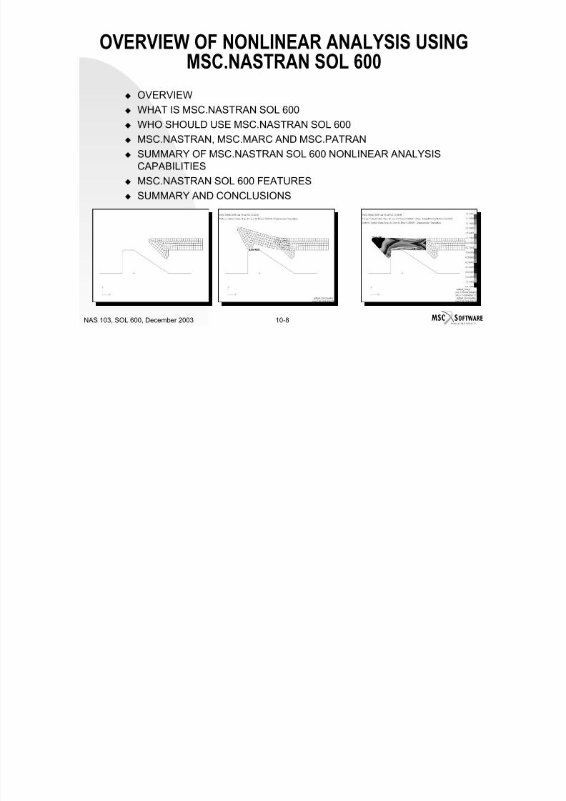
7/21/2019 Nonlinear Analysis Using MSC.nastran
http://slidepdf.com/reader/full/nonlinear-analysis-using-mscnastran 608/783
10-7NAS 103, SOL 600, December 2003
Highly Nonlinear Problems
OVERVIEW OF NONLINEAR ANALYSIS USINGMSC.NASTRAN SOL 600
OVERVIEW WHAT IS MSC.NASTRAN SOL 600
WHO SHOULD USE MSC.NASTRAN SOL 600
MSC.NASTRAN, MSC.MARC AND MSC.PATRAN
SUMMARY OF MSC.NASTRAN SOL 600 NONLINEAR ANALYSISCAPABILITIES
MSC.NASTRAN SOL 600 FEATURES
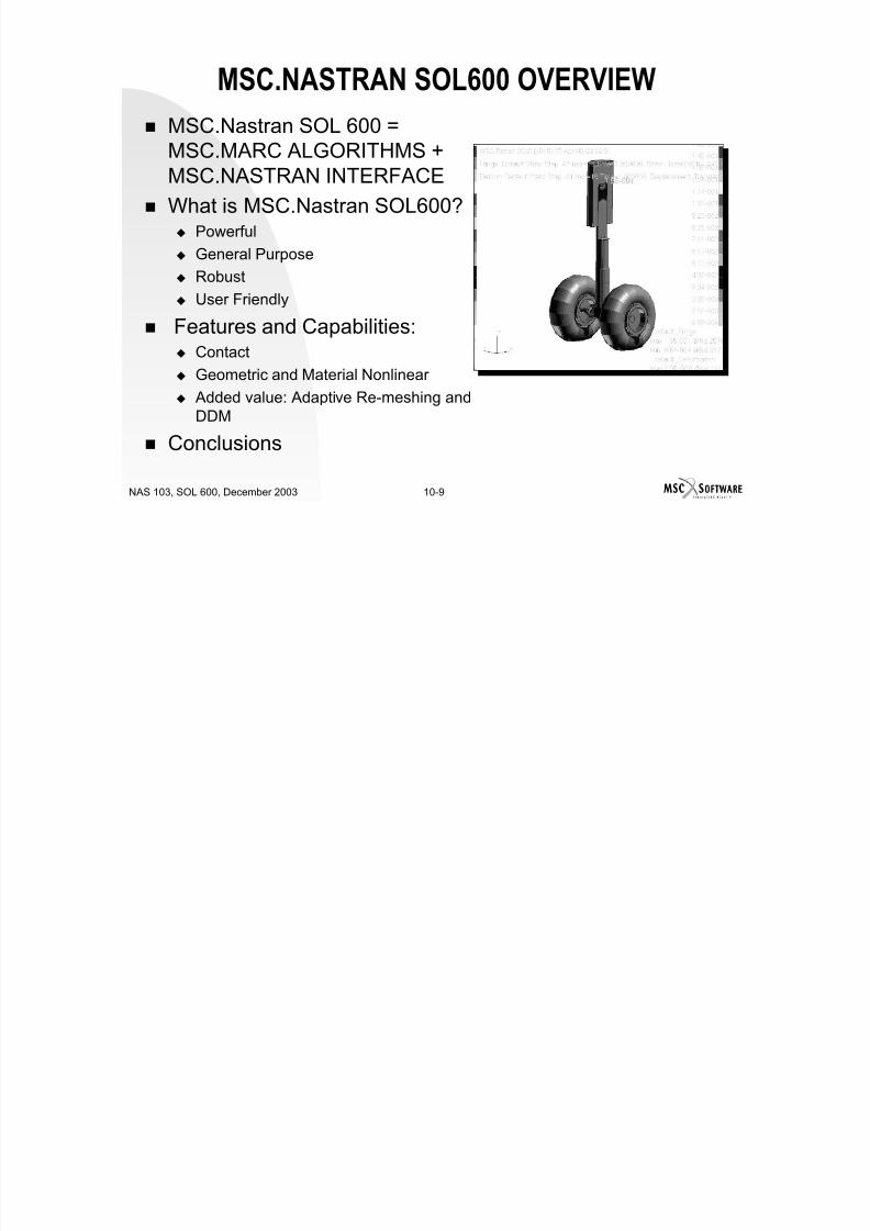
7/21/2019 Nonlinear Analysis Using MSC.nastran
http://slidepdf.com/reader/full/nonlinear-analysis-using-mscnastran 609/783
10-8NAS 103, SOL 600, December 2003
SUMMARY AND CONCLUSIONS
MSC.NASTRAN SOL600 OVERVIEW
MSC.Nastran SOL 600 =
MSC.MARC ALGORITHMS +MSC.NASTRAN INTERFACE
What is MSC.Nastran SOL600?
Powerful General Purpose
Robust
7/21/2019 Nonlinear Analysis Using MSC.nastran
http://slidepdf.com/reader/full/nonlinear-analysis-using-mscnastran 610/783
10-9NAS 103, SOL 600, December 2003
User Friendly
Features and Capabilities: Contact
Geometric and Material Nonlinear
Added value: Adaptive Re-meshing and
DDM Conclusions
WHAT IS MSC.NASTRAN SOL 600?
Integrated Package: MSC.Nastran Interface
MSC.Marc Algorithms
MSC.Patran GUI
Access to most MSC.Marc Capabilities Access to all MSC.Marc Structural / Thermal
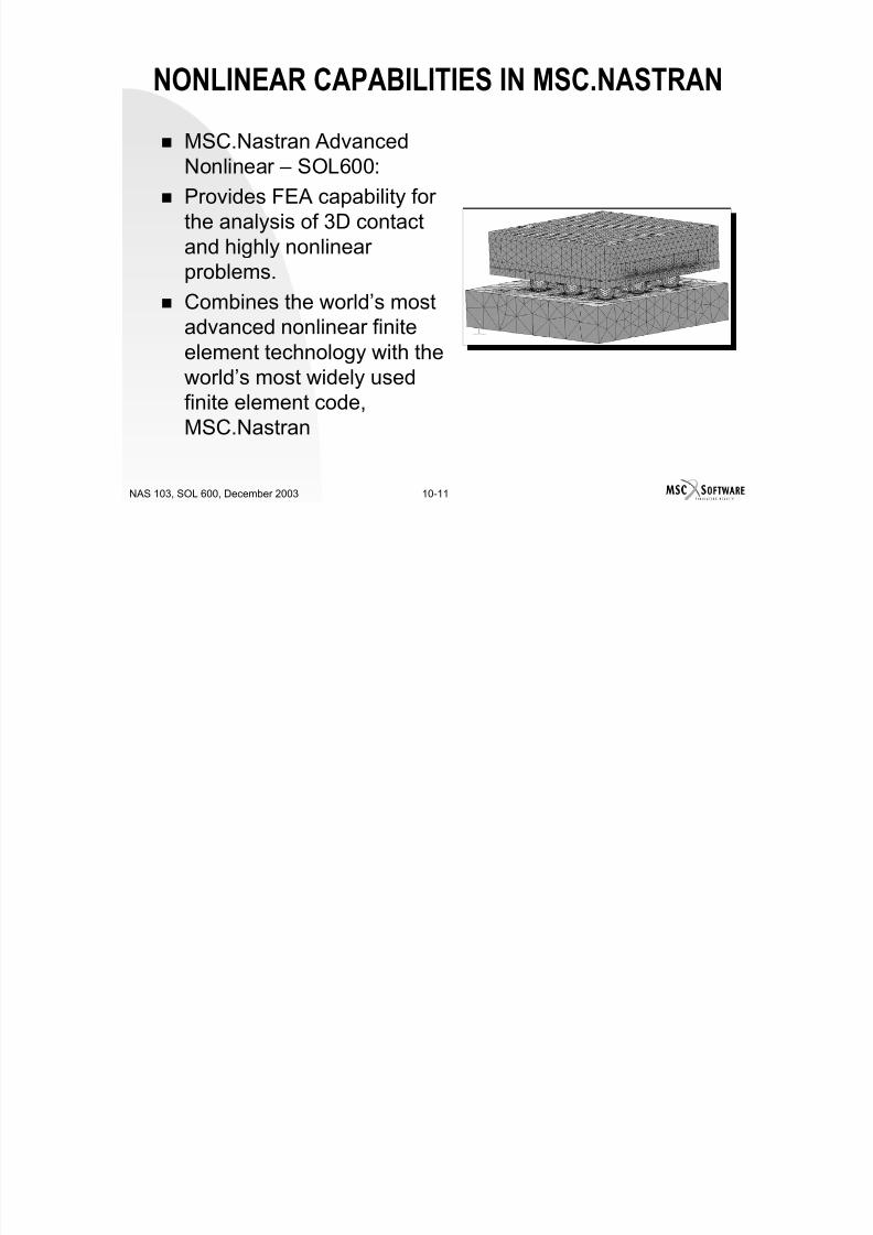
7/21/2019 Nonlinear Analysis Using MSC.nastran
http://slidepdf.com/reader/full/nonlinear-analysis-using-mscnastran 611/783
10-10NAS 103, SOL 600, December 2003
/ Coupled Analysis Capabilities
Easy to Use Intuitive
Powerful
Makes nonlinear finite element analysisEASY!!!
NONLINEAR CAPABILITIES IN MSC.NASTRAN
MSC.Nastran AdvancedNonlinear – SOL600:
Provides FEA capability forthe analysis of 3D contactand highly nonlinearproblems.

7/21/2019 Nonlinear Analysis Using MSC.nastran
http://slidepdf.com/reader/full/nonlinear-analysis-using-mscnastran 612/783
10-11NAS 103, SOL 600, December 2003
Combines the world’s most
advanced nonlinear finiteelement technology with theworld’s most widely usedfinite element code,
MSC.Nastran
WHAT IS MSC.MARC?
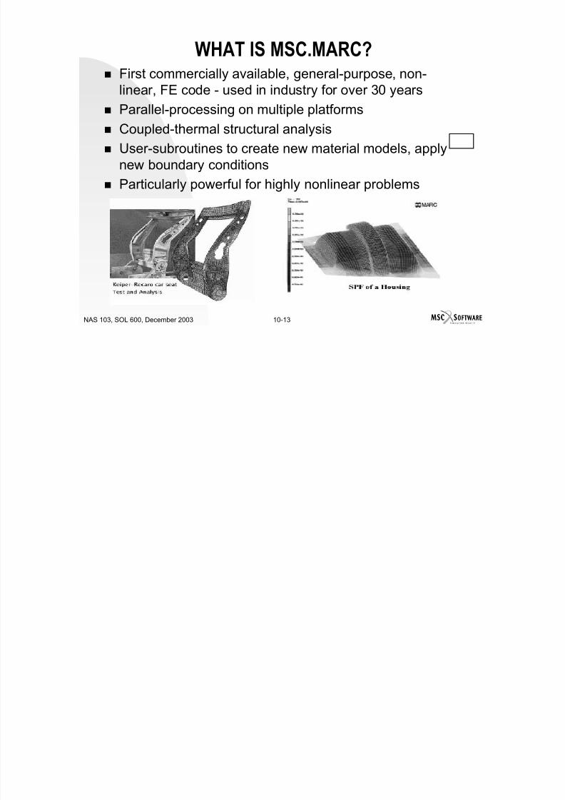
7/21/2019 Nonlinear Analysis Using MSC.nastran
http://slidepdf.com/reader/full/nonlinear-analysis-using-mscnastran 613/783
10-12NAS 103, SOL 600, December 2003
WHAT IS MSC.MARC? First commercially available, general-purpose, non-
linear, FE code - used in industry for over 30 years Parallel-processing on multiple platforms
Coupled-thermal structural analysis
User-subroutines to create new material models, applynew boundary conditions
Particularly powerful for highly nonlinear problems
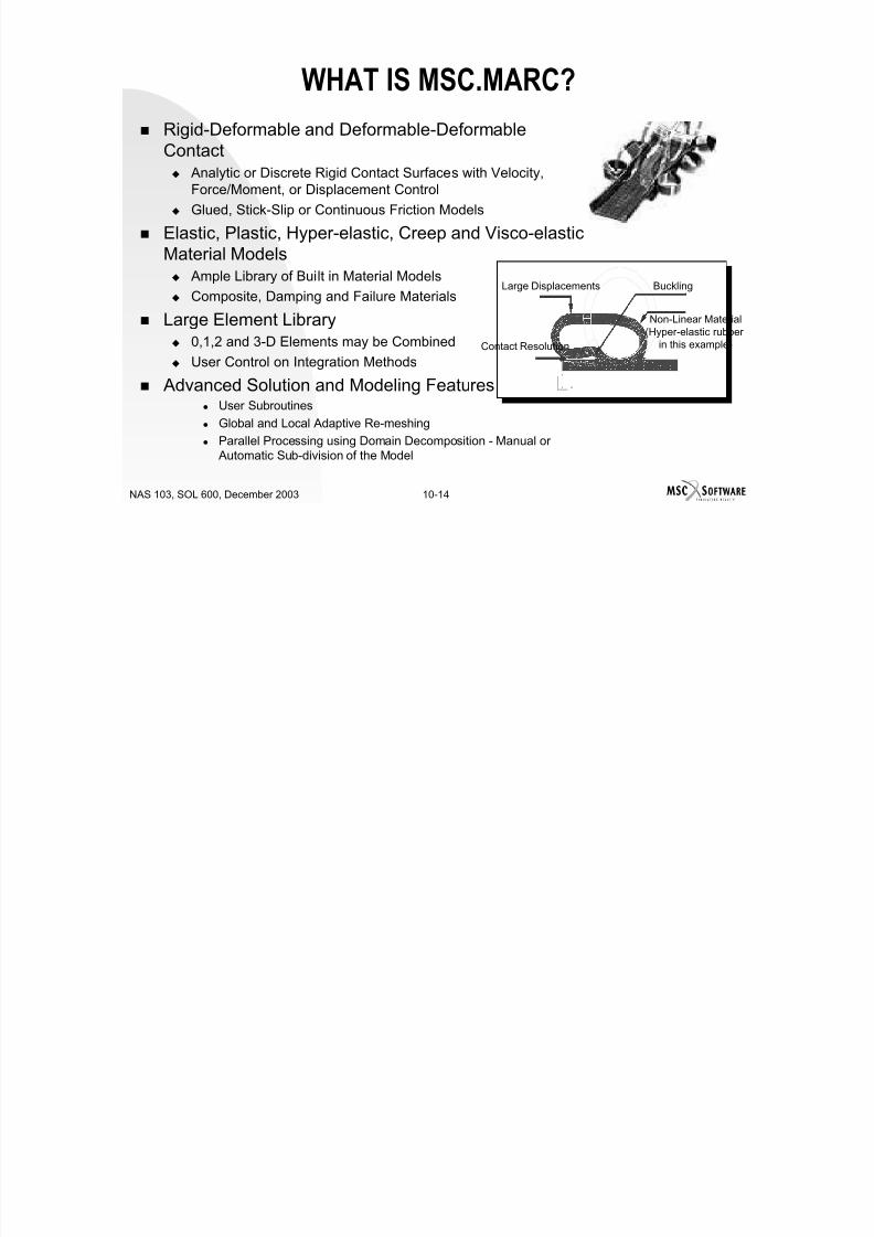
7/21/2019 Nonlinear Analysis Using MSC.nastran
http://slidepdf.com/reader/full/nonlinear-analysis-using-mscnastran 614/783
10-13NAS 103, SOL 600, December 2003
y p g y p
Rigid-Deformable and Deformable-Deformable
Contact Analytic or Discrete Rigid Contact Surfaces with Velocity,
Force/Moment, or Displacement Control
Glued, Stick-Slip or Continuous Friction Models
Elastic, Plastic, Hyper-elastic, Creep and Visco-elasticMaterial Models Ample Library of Built in Material Models
Composite Damping and Failure MaterialsLarge Displacements Buckling
WHAT IS MSC.MARC?
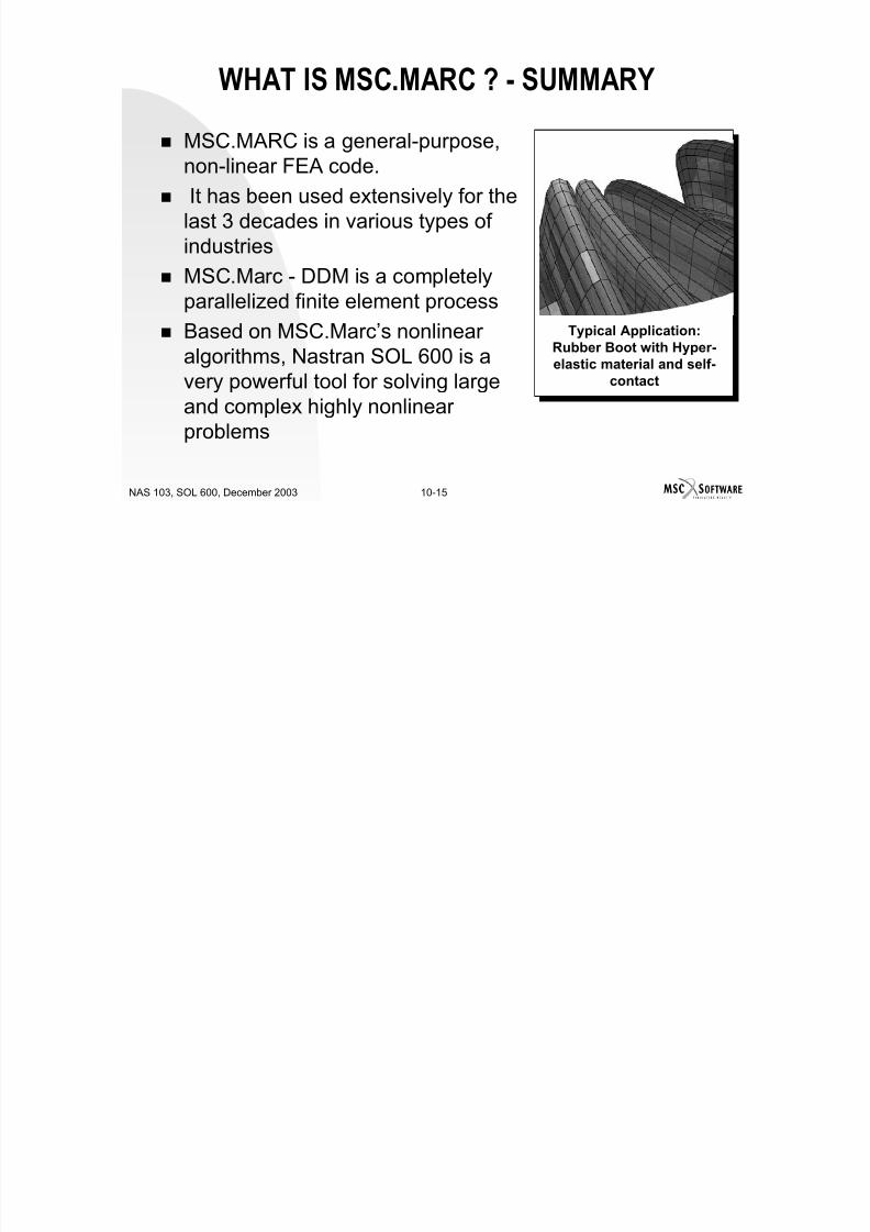
7/21/2019 Nonlinear Analysis Using MSC.nastran
http://slidepdf.com/reader/full/nonlinear-analysis-using-mscnastran 615/783
10-14NAS 103, SOL 600, December 2003
Composite, Damping and Failure Materials
Large Element Library 0,1,2 and 3-D Elements may be Combined
User Control on Integration Methods
Advanced Solution and Modeling Features User Subroutines
Global and Local Adaptive Re-meshing Parallel Processing using Domain Decomposition - Manual or
Automatic Sub-division of the Model
X
Y
Z
Contact Resolution
Non-Linear Material
(Hyper-elastic rubberin this example)
WHAT IS MSC.MARC ? - SUMMARY
MSC.MARC is a general-purpose,non-linear FEA code.
It has been used extensively for thelast 3 decades in various types of
industries MSC.Marc - DDM is a completely
ll li d fi it l t
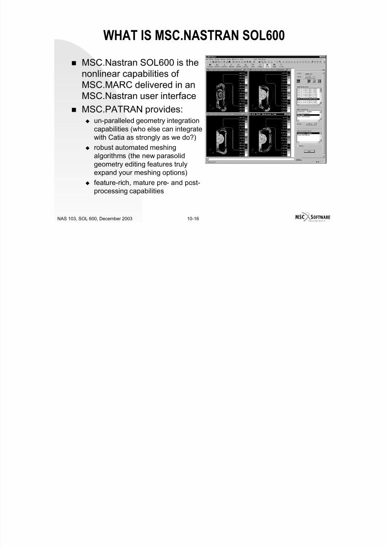
7/21/2019 Nonlinear Analysis Using MSC.nastran
http://slidepdf.com/reader/full/nonlinear-analysis-using-mscnastran 616/783
10-15NAS 103, SOL 600, December 2003
parallelized finite element process
Based on MSC.Marc’s nonlinearalgorithms, Nastran SOL 600 is avery powerful tool for solving largeand complex highly nonlinear
problems
Typical Application:Rubber Boot with Hyper-elastic material and self-
contact
WHAT IS MSC.NASTRAN SOL600
MSC.Nastran SOL600 is thenonlinear capabilities ofMSC.MARC delivered in anMSC.Nastran user interface
MSC.PATRAN provides: un-paralleled geometry integration
capabilities (who else can integrate

7/21/2019 Nonlinear Analysis Using MSC.nastran
http://slidepdf.com/reader/full/nonlinear-analysis-using-mscnastran 617/783
10-16NAS 103, SOL 600, December 2003
p ( gwith Catia as strongly as we do?)
robust automated meshingalgorithms (the new parasolidgeometry editing features trulyexpand your meshing options)
feature-rich, mature pre- and post-
processing capabilities
WHAT IS MSC.PATRAN?
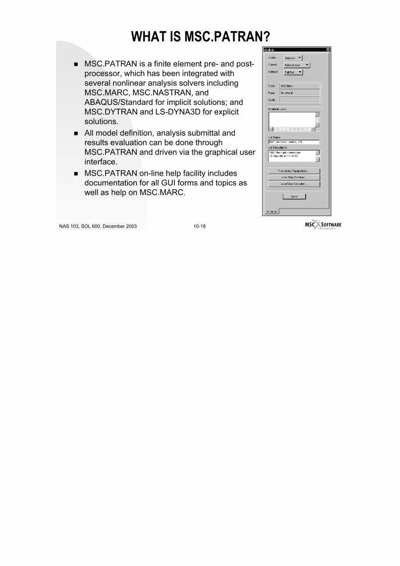
7/21/2019 Nonlinear Analysis Using MSC.nastran
http://slidepdf.com/reader/full/nonlinear-analysis-using-mscnastran 618/783
10-17NAS 103, SOL 600, December 2003
WHAT IS MSC.PATRAN?
MSC.PATRAN is a finite element pre- and post-processor, which has been integrated withseveral nonlinear analysis solvers includingMSC.MARC, MSC.NASTRAN, and ABAQUS/Standard for implicit solutions; and
MSC.DYTRAN and LS-DYNA3D for explicitsolutions.
All model definition, analysis submittal and
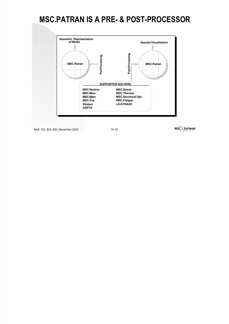
7/21/2019 Nonlinear Analysis Using MSC.nastran
http://slidepdf.com/reader/full/nonlinear-analysis-using-mscnastran 619/783
10-18NAS 103, SOL 600, December 2003
results evaluation can be done through
MSC.PATRAN and driven via the graphical userinterface.
MSC.PATRAN on-line help facility includesdocumentation for all GUI forms and topics as
well as help on MSC.MARC.
MSC.Patran
Geometric Representationof Model
MSC.Patran
P r e - P r o c e
s s i n g
P o s t - P r o c e s s i n g
Results Visualization
MSC.PATRAN IS A PRE- & POST-PROCESSOR
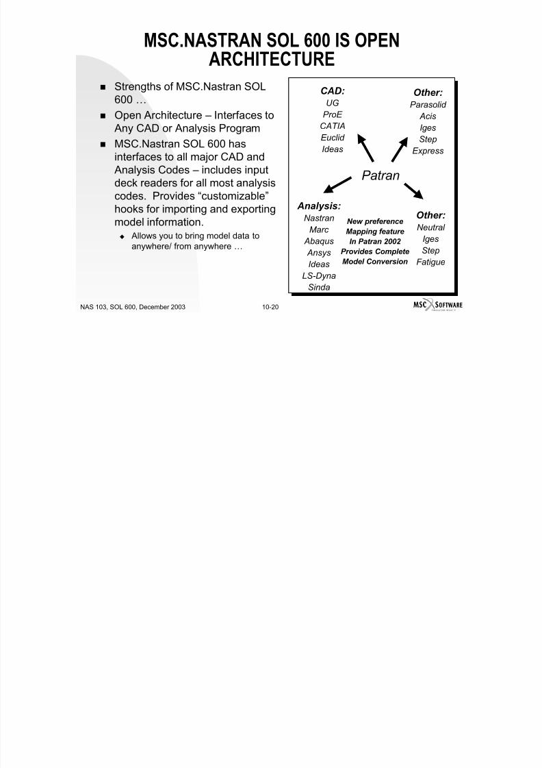
7/21/2019 Nonlinear Analysis Using MSC.nastran
http://slidepdf.com/reader/full/nonlinear-analysis-using-mscnastran 620/783
10-19NAS 103, SOL 600, December 2003
MSC.Nastran
MSC.Marc
MSC.Marc
MSC.Fea
Abaqus
ANSYS
MSC.Dytran
MSC.Thermal
MSC.Structural Opt.
MSC.Fatigue
LS-DYNA3D
SUPPORTED SOLVERS
Patran
CAD:UG
ProE
CATIA
Euclid
Ideas
Other:Parasolid
Acis
Iges
Step
Express
MSC.NASTRAN SOL 600 IS OPENARCHITECTURE
Strengths of MSC.Nastran SOL600 …
Open Architecture – Interfaces to Any CAD or Analysis Program
MSC.Nastran SOL 600 hasinterfaces to all major CAD and Analysis Codes – includes inputdeck readers for all most analysis

7/21/2019 Nonlinear Analysis Using MSC.nastran
http://slidepdf.com/reader/full/nonlinear-analysis-using-mscnastran 621/783
10-20NAS 103, SOL 600, December 2003
Analysis:Nastran
Marc
Abaqus
Ansys
IdeasLS-Dyna
Sinda
Other:
Neutral
Iges
Step
Fatigue
New preference
Mapping feature
In Patran 2002
Provides Complete
Model Conversion
ycodes. Provides “customizable”
hooks for importing and exportingmodel information. Allows you to bring model data to
anywhere/ from anywhere …
WHAT IS MSC.NASTRAN SOL600 ?
Allows Nastran users to perform: nonlinear structural thermal * coupled thermo-structural analysis *
Includes contact, large deflection,
rotation, and strain analysis capabilitiesnever before available in Nastran Can use input decks from the many
thousands of existing MSC.Nastran
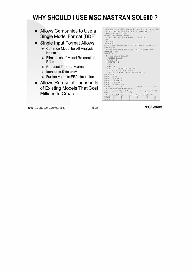
7/21/2019 Nonlinear Analysis Using MSC.nastran
http://slidepdf.com/reader/full/nonlinear-analysis-using-mscnastran 622/783
10-21NAS 103, SOL 600, December 2003
gmodels.
Provides solutions for simple to complexengineering problems including multi-body contact and advanced elastomeric(rubber) material models
* Note: Starred capabilities (on any page) may
not be in first release
WHY SHOULD I USE MSC.NASTRAN SOL600 ?
Allows Companies to Use aSingle Model Format (BDF)
Single Input Format Allows: Common Model for All Analysis
Needs Elimination of Model Re-creation
Effort
Reduced Time to Market
$ NASTRAN input file created by MSC.Nastran input file
$ Direct Text Input for File Management Section$ Nonlinear II Analysis
SOLMARC 600 EXEMARC PATH=3$ Direct Text Input for Executive ControlCENDSEALL = ALL
SUPER = ALLTITLE = MSC.Nastran job created12-Oct-01 at 09:38:33ECHO = NONE$ Direct Text Input for Global Case Control Data
BCONTACT = ALLSUBCASE 1$ Subcase name : Default
SUBTITLE=Default
NLPARM = 1BCONTACT = 1
SPC = 2LOAD = 2
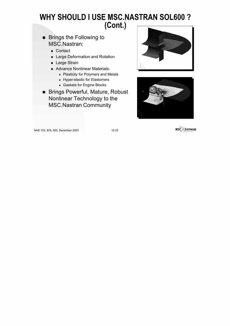
7/21/2019 Nonlinear Analysis Using MSC.nastran
http://slidepdf.com/reader/full/nonlinear-analysis-using-mscnastran 623/783
10-22NAS 103, SOL 600, December 2003
Reduced Time-to-Market
Increased Efficiency Further value to FEA simulation
Allows Re-use of Thousandsof Existing Models That Cost
Millions to Create
DISPLACEMENT(SORT1,REAL)=ALL
SPCFORCES(SORT1,REAL)=ALL
STRESS(SORT1,REAL,VONMISES,BILIN)=ALLBEGIN BULKPARAM POST 0PARAM AUTOSPC NO
PARAM LGDISP 1PARAM,NOCOMPS,-1PARAM PRTMAXIM YESNLPARM 1 10 AUTO 5 25
$ Direct Text Input for Bulk Data$ Elements and Element Properties for region : shell
PSHELL 1 1 .25 1 1$ Pset: "shell" will be imported as: "pshell.1"CQUAD4 1 1 1 2 13 12
CQUAD4 2 1 2 3 14 13
WHY SHOULD I USE MSC.NASTRAN SOL600 ?(Cont.)
Brings the Following toMSC.Nastran: Contact
Large Deformation and Rotation
Large Strain Advance Nonlinear Materials:
Plasticity for Polymers and Metals
Hyper-elastic for Elastomers
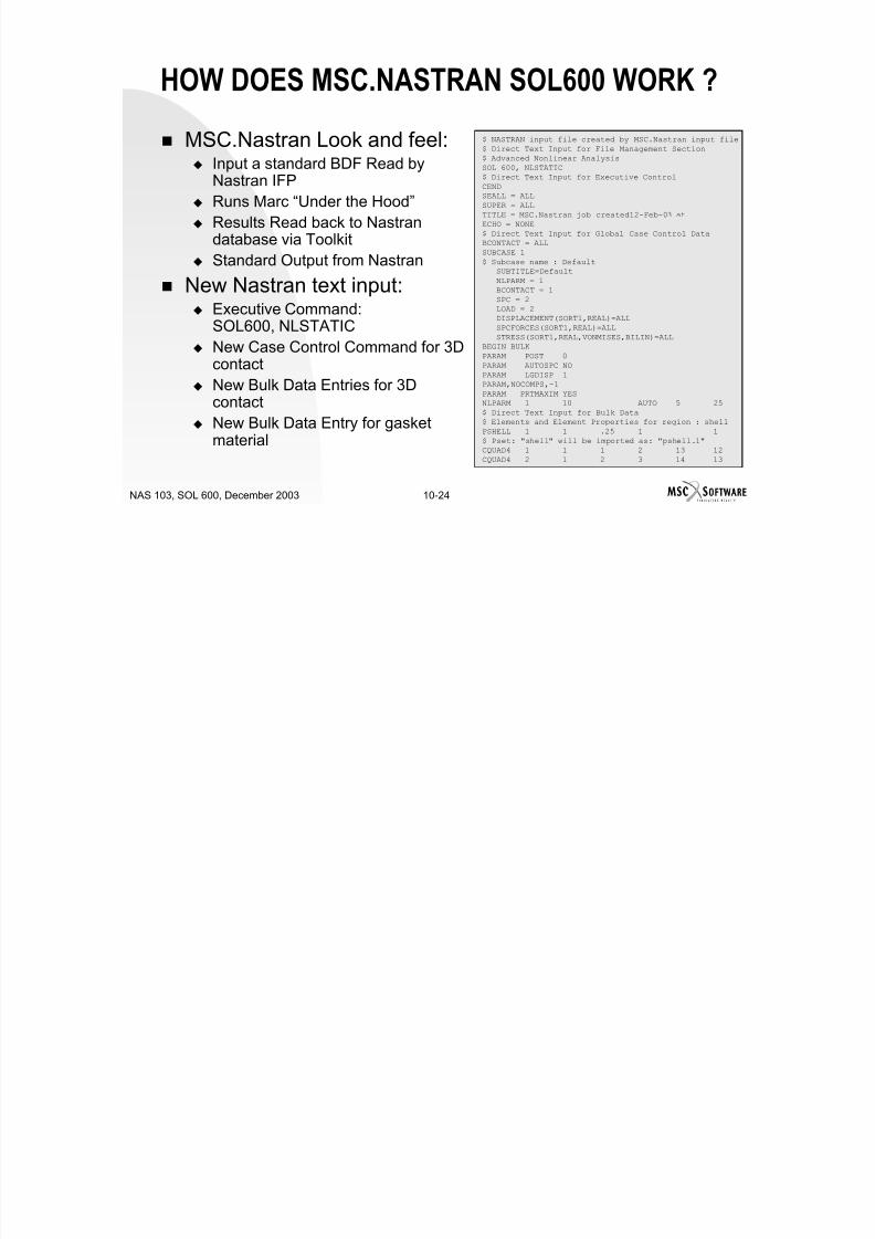
7/21/2019 Nonlinear Analysis Using MSC.nastran
http://slidepdf.com/reader/full/nonlinear-analysis-using-mscnastran 624/783
10-23NAS 103, SOL 600, December 2003
yp
Gaskets for Engine Blocks
Brings Powerful, Mature, RobustNonlinear Technology to theMSC.Nastran Community
HOW DOES MSC.NASTRAN SOL600 WORK ?
MSC.Nastran Look and feel: Input a standard BDF Read byNastran IFP
Runs Marc “Under the Hood” Results Read back to Nastran
database via Toolkit Standard Output from Nastran
New Nastran text input: Executive Command:
$ NASTRAN input file created by MSC.Nastran input file
$ Direct Text Input for File Management Section$ Advanced Nonlinear AnalysisSOL 600, NLSTATIC$ Direct Text Input for Executive Control
CENDSEALL = ALL
SUPER = ALLTITLE = MSC.Nastran job created12-Feb-03 atECHO = NONE
$ Direct Text Input for Global Case Control Data
BCONTACT = ALLSUBCASE 1
$ Subcase name : DefaultSUBTITLE=Default
NLPARM = 1BCONTACT = 1SPC = 2LOAD = 2
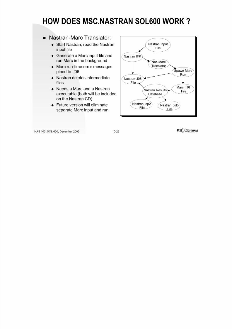
7/21/2019 Nonlinear Analysis Using MSC.nastran
http://slidepdf.com/reader/full/nonlinear-analysis-using-mscnastran 625/783
10-24NAS 103, SOL 600, December 2003
Executive Command:SOL600, NLSTATIC
New Case Control Command for 3Dcontact
New Bulk Data Entries for 3Dcontact
New Bulk Data Entry for gasketmaterial
LOAD = 2DISPLACEMENT(SORT1,REAL)=ALL
SPCFORCES(SORT1,REAL)=ALL
STRESS(SORT1,REAL,VONMISES,BILIN)=ALLBEGIN BULKPARAM POST 0
PARAM AUTOSPC NOPARAM LGDISP 1PARAM,NOCOMPS,-1
PARAM PRTMAXIM YESNLPARM 1 10 AUTO 5 25
$ Direct Text Input for Bulk Data$ Elements and Element Properties for region : shell
PSHELL 1 1 .25 1 1$ Pset: "shell" will be imported as: "pshell.1"CQUAD4 1 1 1 2 13 12
CQUAD4 2 1 2 3 14 13
HOW DOES MSC.NASTRAN SOL600 WORK ?
Nastran-Marc Translator: Start Nastran, read the Nastran
input file
Generate a Marc input file andrun Marc in the background
Marc run-time error messagespiped to .f06
Nastran deletes intermediatefiles
Nastran InputFile
Nastran IFP
Nas-MarcTranslator
Spawn MarcRun
Nastran .f06File
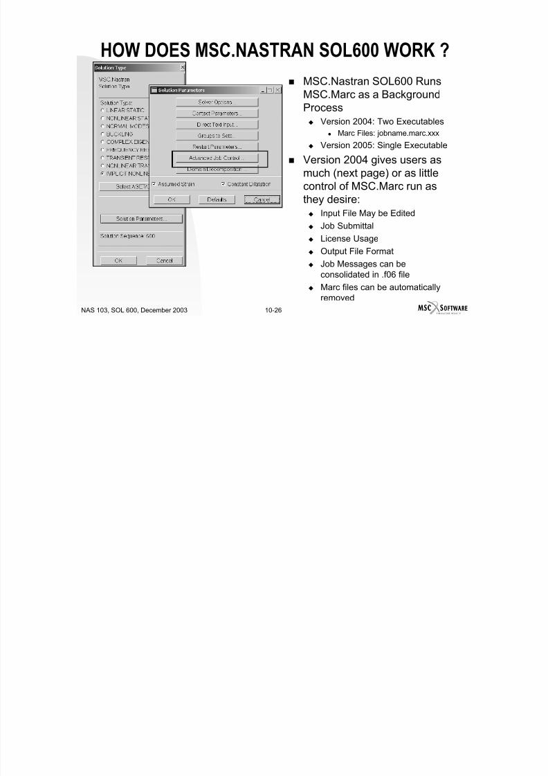
7/21/2019 Nonlinear Analysis Using MSC.nastran
http://slidepdf.com/reader/full/nonlinear-analysis-using-mscnastran 626/783
10-25NAS 103, SOL 600, December 2003
files
Needs a Marc and a Nastranexecutable (both will be includedon the Nastran CD)
Future version will eliminateseparate Marc input and run
Nastran ResultsDatabase
File
Marc .t16File
Nastran .xdbFile
Nastran .op2File
MSC.Nastran SOL600 Runs
MSC.Marc as a BackgroundProcess Version 2004: Two Executables
Marc Files: jobname.marc.xxx
Version 2005: Single Executable
Version 2004 gives users asmuch (next page) or as littlecontrol of MSC.Marc run asth d i
HOW DOES MSC.NASTRAN SOL600 WORK ?
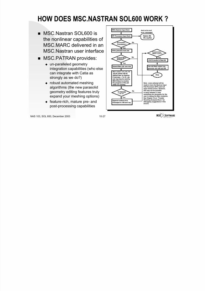
7/21/2019 Nonlinear Analysis Using MSC.nastran
http://slidepdf.com/reader/full/nonlinear-analysis-using-mscnastran 627/783
10-26NAS 103, SOL 600, December 2003
they desire: Input File May be Edited Job Submittal
License Usage
Output File Format
Job Messages can beconsolidated in .f06 file
Marc files can be automaticallyremoved
HOW DOES MSC.NASTRAN SOL600 WORK ?
MSC.Nastran SOL600 isthe nonlinear capabilities ofMSC.MARC delivered in anMSC.Nastran user interface
MSC.PATRAN provides: un-paralleled geometry
integration capabilities (who elsecan integrate with Catia as
MSC.Nastran Input Deck
Use std Nast output req -
deck echo and
Write jobname.marc.dat
IFP Processes Input Deck
SuccessfulTranslation?
Submit MarcAnalysis?
Marc writes .out,.t16,.t19
Post-processingDMAP in place?
Submit Marc job -see note
.t16/19 results to Nast db
Nastran .f06,
.f04, .log files
error messages
Yes
Yes
Yes
generate std xdb,op2,f06
sts etc (these will be
No
No
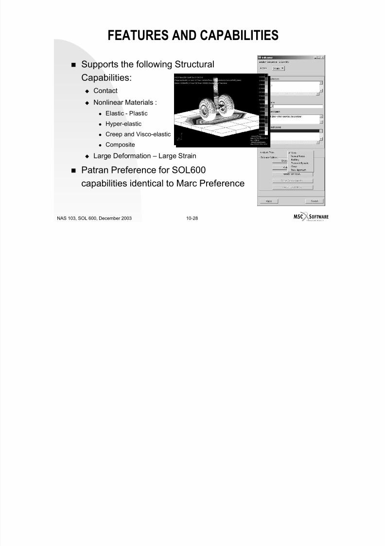
7/21/2019 Nonlinear Analysis Using MSC.nastran
http://slidepdf.com/reader/full/nonlinear-analysis-using-mscnastran 628/783
10-27NAS 103, SOL 600, December 2003
can integrate with Catia as
strongly as we do?) robust automated meshing
algorithms (the new parasolidgeometry editing features trulyexpand your meshing options)
feature-rich, mature pre- andpost-processing capabilities
Stop
Is marccpy= 1or 2?
Append runtime error
Yes
.sts,etc (these will bedeleted later by Nastranif marccpy = 1 or 3) -.sts
messages to .f06 and .log
and .log may be used byMSC.Patran to monitorthe progress of the jobwhile it is running
Note - every attempt will be
made to have the Nastran InputFile Processor (IFP) catch allinput format errors. However,this may not be possible
in early releases. It maysometimes be necessary for theuser to debug the Marc analyisis.
See Chapter 16 on “TroubleShooting Analysis Runs” for
debugging suggestions if thisoccurs.
No
FEATURES AND CAPABILITIES
Supports the following StructuralCapabilities: Contact
Nonlinear Materials :
Elastic - Plastic
Hyper-elastic
Creep and Visco-elastic
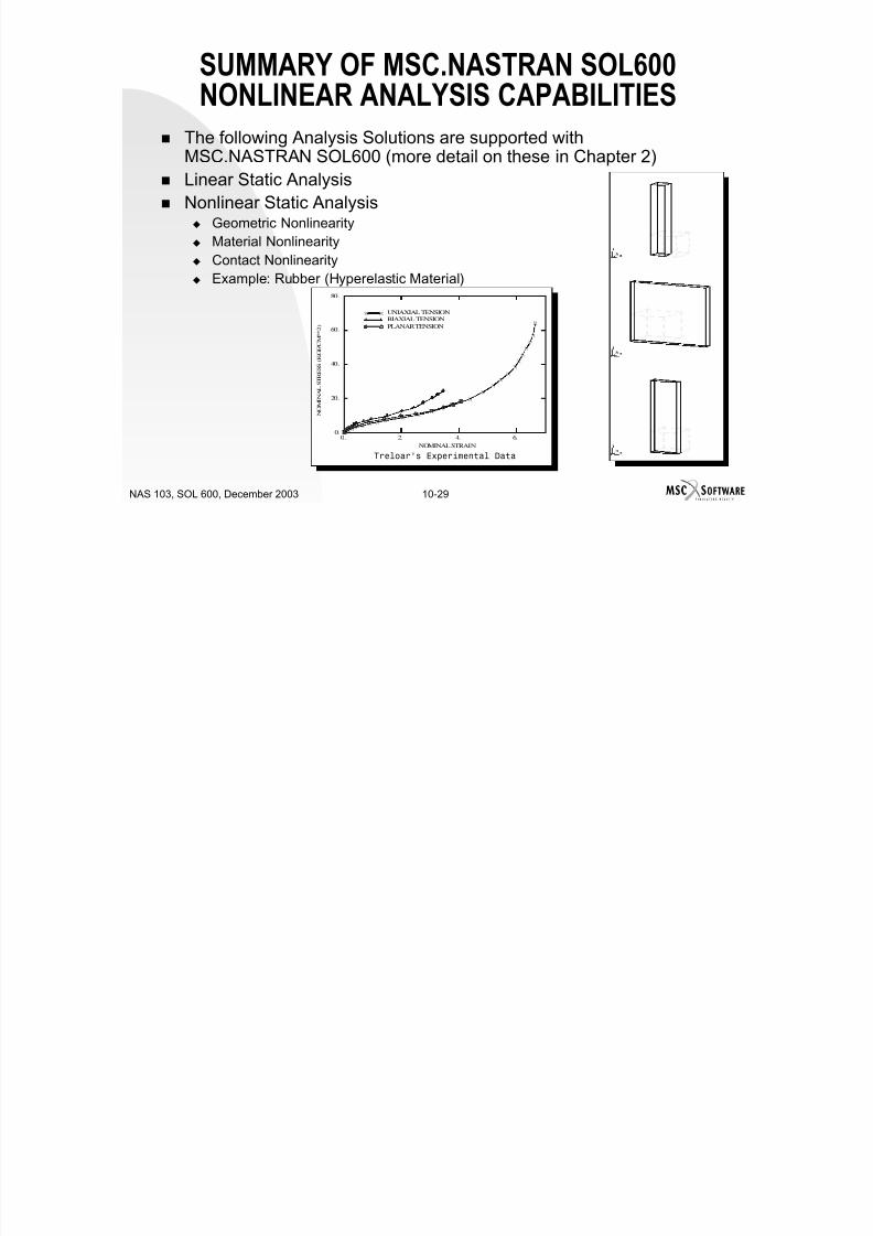
7/21/2019 Nonlinear Analysis Using MSC.nastran
http://slidepdf.com/reader/full/nonlinear-analysis-using-mscnastran 629/783
10-28NAS 103, SOL 600, December 2003
Composite
Large Deformation – Large Strain
Patran Preference for SOL600
capabilities identical to Marc Preference
1
23
1
23
80.
UNIAXIAL TENSION
SUMMARY OF MSC.NASTRAN SOL600NONLINEAR ANALYSIS CAPABILITIES
The following Analysis Solutions are supported withMSC.NASTRAN SOL600 (more detail on these in Chapter 2)
Linear Static Analysis Nonlinear Static Analysis
Geometric Nonlinearity
Material Nonlinearity Contact Nonlinearity Example: Rubber (Hyperelastic Material)

7/21/2019 Nonlinear Analysis Using MSC.nastran
http://slidepdf.com/reader/full/nonlinear-analysis-using-mscnastran 630/783
10-29NAS 103, SOL 600, December 2003
1
23
1
23
1
23
1
23
0. 2. 4. 6.
NOMINAL STRAIN
0.
20.
40.
60.
BIAXIAL TENSION
PLANAR TENSION
Treloar’s Experimental Data
N O M I N A L S T R E S S ( K G F / C M * * 2 )
NON-LINEAR CAPABILITIES IN MSC.NASTRANSOL600
Materially Non-linearModels
Geometric Non-linearity's
Boundary Condition Non-linearity's (Contact)
All Non-linear BehaviorsCan be Combined …
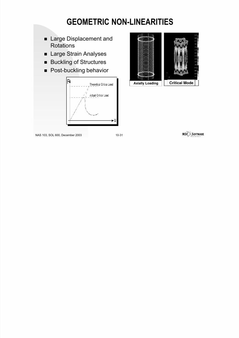
7/21/2019 Nonlinear Analysis Using MSC.nastran
http://slidepdf.com/reader/full/nonlinear-analysis-using-mscnastran 631/783
10-30NAS 103, SOL 600, December 2003
Example Application: BallJoint
Axi-symmetric model
of ball-joint assembly
GEOMETRIC NON-LINEARITIES
Large Displacement andRotations
Large Strain Analyses
Buckling of Structures
Post-buckling behavior
Axially Loading Critical Mode

7/21/2019 Nonlinear Analysis Using MSC.nastran
http://slidepdf.com/reader/full/nonlinear-analysis-using-mscnastran 632/783
10-31NAS 103, SOL 600, December 2003
GEOMETRIC NONLINEARITY - FINITEDEFORMATION
Finite Deformation Large Deflection, Rotation andStrain: Large Deformation and Rotation of RBE’S Large (Finite) Strain With Choice of Strain
Definitions Finite Strain Plasticity
Robust and User-FriendlyAdaptive Load Incrementation
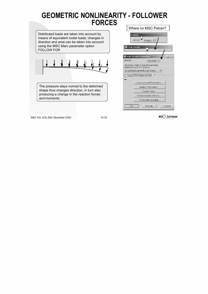
7/21/2019 Nonlinear Analysis Using MSC.nastran
http://slidepdf.com/reader/full/nonlinear-analysis-using-mscnastran 633/783
10-32NAS 103, SOL 600, December 2003
Adaptive Load Incrementation Total and Updated Lagrange
Procedures Choice of Solvers Including
Iterative and MSC.Nastran’s FastSparse
Distributed loads are taken into account bymeans of equivalent nodal loads; changes indirection and area can be taken into accountusing the MSC.Marc parameter optionFOLLOW FOR
Where on MSC.Patran?
GEOMETRIC NONLINEARITY - FOLLOWERFORCES
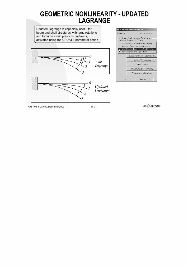
7/21/2019 Nonlinear Analysis Using MSC.nastran
http://slidepdf.com/reader/full/nonlinear-analysis-using-mscnastran 634/783
10-33NAS 103, SOL 600, December 2003
The pressure stays normal to the deformedshape thus changes direction, in turn alsoproducing a change in the reaction forcesand moments.
Updated Lagrange is especially useful for
beam and shell structures with large rotationsand for large strain plasticity problems;activated using the UPDATE parameter option
0
1
2
Total Lagrange
GEOMETRIC NONLINEARITY - UPDATEDLAGRANGE

7/21/2019 Nonlinear Analysis Using MSC.nastran
http://slidepdf.com/reader/full/nonlinear-analysis-using-mscnastran 635/783
10-34NAS 103, SOL 600, December 2003
3
0
1
23
Updated Lagrange
Isotropic 2-D and 3-D Orthotropic 2-D and 3-D Anisotropic Laminated and 3D
Composites, Gaskets forEngine Blocks Material properties can be
temperature dependent e.g.
MSC.NASTRAN SOL600 MATERIALS

7/21/2019 Nonlinear Analysis Using MSC.nastran
http://slidepdf.com/reader/full/nonlinear-analysis-using-mscnastran 636/783
10-35NAS 103, SOL 600, December 2003
Young’s Modulus Poisson Ratio Coefficient of Thermal Expansion Specific Heat Thermal Conductivity And more…
MSC.NASTRAN SOL600 PLASTICITY MODELS
Perfectly Plastic and Rigid Plastic
Elastic Plastic with Hardening orSoftening
Plastic - Hardening Laws: Isotropic
Kinematic
Combined and others
Plastic - Yielding: With a dependence of the yield stress

7/21/2019 Nonlinear Analysis Using MSC.nastran
http://slidepdf.com/reader/full/nonlinear-analysis-using-mscnastran 637/783
10-36NAS 103, SOL 600, December 2003
p y
on strain rate Von Mises and Drucker-Prager
Linear and Parabolic Mohr-Coulomb
Various Oak Ridge National Laboratorymodels and others
Hyper-elastic Including Graphical Feedback on
Experimental Data Fitting
Large strain for elastic materials(rubber) using; Neo-Hookean
Mooney-Rivlin
Ogden
Gent
SOL600 HYPERELASITIC MODELS

7/21/2019 Nonlinear Analysis Using MSC.nastran
http://slidepdf.com/reader/full/nonlinear-analysis-using-mscnastran 638/783
10-37NAS 103, SOL 600, December 2003
Arruda-Boyce Jamus-Green-Simpson models
Large strain, elastic analysis ofcompressible foams
Nonlinear Material Models Creep
Behavior for materials where, for aconstant stress state, strainincreases with time
Relaxation where stress decreases
with time at constant deformation Visco-elastic
Behavior for elastic materials thatrelax and dissipate energy undertransient loadings
NONLINEAR MATERIAL MODELS

7/21/2019 Nonlinear Analysis Using MSC.nastran
http://slidepdf.com/reader/full/nonlinear-analysis-using-mscnastran 639/783
10-38NAS 103, SOL 600, December 2003
Failure Hill, Hoffman, Tsai-Wu, MaximumStress or Strain
Damping Using Mass or Stiffness Matrix, or
Numerical Multipliers - can be used
together
BOUNDARY CONDITION NON-LINEARITY
Contact Developed in Marc in late ’80s
Automatic detection of contact
2D and 3D contact
Finds widespread use in areas likeManufacturing Simulations for sheetmetal forming, deep drawing, mountingseals and other process simulations,bio- medical simulations and more

7/21/2019 Nonlinear Analysis Using MSC.nastran
http://slidepdf.com/reader/full/nonlinear-analysis-using-mscnastran 640/783
10-39NAS 103, SOL 600, December 2003
BOUNDARY CONDITION NON-LINEARITY
Contact Automatic Re-meshing during contact
Friction models Stick-slip model
Coloumb model
Shear Friction for rolling

7/21/2019 Nonlinear Analysis Using MSC.nastran
http://slidepdf.com/reader/full/nonlinear-analysis-using-mscnastran 641/783
10-40NAS 103, SOL 600, December 2003
RIGID & DEFORMABLE BODIES
Analytic or Discrete Rigid Contact Surfaces with Velocity,Force/Moment, or Displacement Control
Glued, Stick-Slip or Continuous Friction Models

7/21/2019 Nonlinear Analysis Using MSC.nastran
http://slidepdf.com/reader/full/nonlinear-analysis-using-mscnastran 642/783
10-41NAS 103, SOL 600, December 2003
MSC.NASTRAN SOL600 CONTACT
Contact Capabilities Brings Advanced Contact
Capabilities to MSC.Nastran: Easy to Use Multi-Body Capability
2-D and Full 3-D Contact Supports Rigid-Deformable Contact
Position, Velocity or Load ControlledRigid Bodies
Rigid Geometry Defined Via NURBS DeformableContact stress
Contact area

7/21/2019 Nonlinear Analysis Using MSC.nastran
http://slidepdf.com/reader/full/nonlinear-analysis-using-mscnastran 643/783
10-42NAS 103, SOL 600, December 2003
g y
Discrete or Analytical DefinitionDeformableStructure (including friction)
Calculated
MSC.NASTRAN SOL600 CONTACT
Contact Capabilities Include Deformable-Deformable Contact With:
Initial Interference Fit
Stress – Free Initial Mesh Adjustment Single or Double – Sided Contact
Detection Force or Stress–Based Separation
Multiple Friction Models

7/21/2019 Nonlinear Analysis Using MSC.nastran
http://slidepdf.com/reader/full/nonlinear-analysis-using-mscnastran 644/783
10-43NAS 103, SOL 600, December 2003
Glued Contact Automatic or User – Defined
Contact Tolerance Distance
(CTD) Bias on CTD
BOUNDARY CONDITION NON-LINEARITY
Multi-Body Contact Very Easy to Set-Up
Automatic detection of contact surfaces
2D and 3D contact
Finds widespread use in areaslike: Manufacturing Simulationsfor sheet metal forming, deepdrawing, mounting seals and

7/21/2019 Nonlinear Analysis Using MSC.nastran
http://slidepdf.com/reader/full/nonlinear-analysis-using-mscnastran 645/783
10-44NAS 103, SOL 600, December 2003
other process simulations, bio-medical simulations and more
Try setting this up with contactpair contact …
BOUNDARY CONDITION NON-LINEARITY
Contact Capabilities: Rigid and Deformable
Automatic Re-meshing duringcontact
Reports Interface Results
Surface Interactions Contact Distance Tol
Bias on Distance Tol
Quadratic Elements

7/21/2019 Nonlinear Analysis Using MSC.nastran
http://slidepdf.com/reader/full/nonlinear-analysis-using-mscnastran 646/783
10-45NAS 103, SOL 600, December 2003
Friction models Glued Contact
Separation Force
EXAMPLE - ANALYSIS OF A RUBBER BOOT
All Non-Linearities Can Appear Together
Constant Velocity Rubber Boot Elastomeric material model (Mooney, non-linear elastic)
Large rotations and strains
Multi-body and Self-contact (default) Local buckling

7/21/2019 Nonlinear Analysis Using MSC.nastran
http://slidepdf.com/reader/full/nonlinear-analysis-using-mscnastran 647/783
10-46NAS 103, SOL 600, December 2003
MSC.NASTRAN SOL 600 FEATURES
MSC.NASTRAN SOL 600 Features: Structural, Thermal and Coupled
Analysis (thermal and coupled in2004)
Material, Geometric and Contact
Non-linearity Parallel Processing (DMP)
available (in 2003)
Experimental Data fitting for elastomers (in 2003)

7/21/2019 Nonlinear Analysis Using MSC.nastran
http://slidepdf.com/reader/full/nonlinear-analysis-using-mscnastran 648/783
10-47NAS 103, SOL 600, December 2003
User Defined Subroutines (2004)
Global Re-meshing (2004)
FEATURES - MATRIX SOLVER OPTIONS
Matrix Solution Methods (more on this later) Direct Solver
Direct Sparse
Iterative Solver (Conjugate Gradient)
Sparse Iterative
New BCS Solver (Multi-frontal solver)

7/21/2019 Nonlinear Analysis Using MSC.nastran
http://slidepdf.com/reader/full/nonlinear-analysis-using-mscnastran 649/783
10-48NAS 103, SOL 600, December 2003
FEATURES – DISTRIBUTED MEMORYPARALLEL
MSC.Nastran DMP Parallel Processing
Automatic Subdivision based on Metis
Manual Decomposition based on MSC.PatranGroups
Nastran SOL 600 allows DMP using a singleinput file

7/21/2019 Nonlinear Analysis Using MSC.nastran
http://slidepdf.com/reader/full/nonlinear-analysis-using-mscnastran 650/783
10-49NAS 103, SOL 600, December 2003
1 CPU 4 CPUs
PARALLEL PROCESSING: DISTRIBUTEDMEMORY PARALLEL METHOD
Mesh is broken up into several domains, each submittedto a different CPU

7/21/2019 Nonlinear Analysis Using MSC.nastran
http://slidepdf.com/reader/full/nonlinear-analysis-using-mscnastran 651/783
10-50NAS 103, SOL 600, December 2003
Linearly-Scalable Distributed
Memory Parrallel MSC.Nastran SOL600 DMP often
gives what is called “Super-Linear”scalability – meaning the you getbetter than 1/# cpu performance
increase. This occurs because the% of in-core solution time goes wayup …
In a recent comparisonMSC.Nastran SOL600’s DMP
bili d l
PARALLEL PROCESSING: DISTRIBUTEDMEMORY PARALLEL METHOD

7/21/2019 Nonlinear Analysis Using MSC.nastran
http://slidepdf.com/reader/full/nonlinear-analysis-using-mscnastran 652/783
10-51NAS 103, SOL 600, December 2003
capability was used to solve anengine block problem in 2.5 hoursthat took our competitor 7 days tosolve using a single cpu solution.
Who wouldn’t want to cut their
solution times down by an order ofmagnitude …
Domain 1 Domain 2
Domain 3
Domain 4
Entire Engine ModelGenerally linear scaling!
FEATURES - DISTRIBUTED MEMORYPARALLEL
Example 448,361 Elements
1.8 Million DOFs
10 Increment -
Transient Thermal
Analysis 78 minute on single
processor
12 minutes on 8 CPUs

7/21/2019 Nonlinear Analysis Using MSC.nastran
http://slidepdf.com/reader/full/nonlinear-analysis-using-mscnastran 653/783
10-52NAS 103, SOL 600, December 2003
Domain 5Domain 6
Domain 7Domain 8
FEATURES - ADVANCED ELEMENTTECHNOLOGY
Advanced ElementTechnology Linear and Quadratic
Herrmann Formulation forIncompressible Materials
Assumed Strain – CapturesStress Distribution in Bending
Global and Local Adaptive Re-meshing
P ll l P i i
Linear
Quadratic
Mid-body (Hermann formulation)

7/21/2019 Nonlinear Analysis Using MSC.nastran
http://slidepdf.com/reader/full/nonlinear-analysis-using-mscnastran 654/783
10-53NAS 103, SOL 600, December 2003
Parallel Processing usingDISTRIBUTED MEMORYPARALLEL - Manual or AutomaticSub-division of the Model
User Subroutines
Mid-body (Hermann formulation)
FEATURES - CONCLUSION
Take advantage of the MSC.Marcfeatures through an MSC.Nastraninterface:
1. Easy to Set-up Multi-body Contact
2. Global adaptive re-meshing
3. Experimental data fitting with graphical userfeedback
4. Linearly scalable DDM 300150 450 600 750 900Strain
S t r e s s
15
30
45
60
75

7/21/2019 Nonlinear Analysis Using MSC.nastran
http://slidepdf.com/reader/full/nonlinear-analysis-using-mscnastran 655/783
10-54NAS 103, SOL 600, December 2003
Domain 1 Domain 2
Domain 3
Domain 4
448,361 Elements1.8 Million DOFs10 Increment -TransientThermal Analysis78 min. on single
processor 12 minutes on 8CPUs
1.0A B
SUMMARY OF MSC.NASTRAN SOL 600NONLINEAR ANALYSIS CAPABILITIES
General Solution Features No fixed problem size limits, DISTRIBUTED MEMORY PARALLEL avail.
for parallel solution
Automated procedures for load step, convergence control, andequilibrium/stability control in nonlinear analysis
Reliable Newton-Raphson algorithm Arc length control for static collapse problems

7/21/2019 Nonlinear Analysis Using MSC.nastran
http://slidepdf.com/reader/full/nonlinear-analysis-using-mscnastran 656/783
10-55NAS 103, SOL 600, December 2003
Load, P
Displacement
Proportional loading with unstable response.
WHEN TO USE SOL600 VS 106/129
Most Common Reasons to Use MSC.Nastran SOL 600:Capability SOL 106/129 SOL 600
2D Def-Def Contact Slidelines Multi-Body
2D Rigid-Def Contact No Multi-Body
3D Def-Def Contact Slidelines Multi-Body
3D Rigid-Def Contact No Multi-Body
Beam Contact No Multi-Body
Elastic-Perfectly Plastic via Bi-Linear Yes
Bi-linear Elastic Plastic Yes via Multi-Linear
Multi-linear Elastic Plastic Yes Yes
Temp-Dependent Elastic-Plastic No Yes
Multi-linear Elastic Yes No
Mooney-Rivlin for 1D (beam) elements No Yes
Mooney-Rivlin for 2D elements Yes YesMooney-Rivlin for 3D elements Yes Yes
Need to Model 3D or Multi-BodyContact
Strain Level > 10-15%
RBE’s/MPC’s need large
rotation capability Elastic-Plastic or Hyper-Elastic
Material Properties areTemperature Dependent
Need to Model 3D SolidComposites

7/21/2019 Nonlinear Analysis Using MSC.nastran
http://slidepdf.com/reader/full/nonlinear-analysis-using-mscnastran 657/783
10-56NAS 103, SOL 600, December 2003
Mooney-Rivlin for 3D elements Yes Yes
Other hyperelastic (Ogden,Gent…) for all
element types No Yes
Temp-Dependent Hyperelastic No Yes
Composite Beams Yes Yes
Composite Shells Yes Yes
Continuum (2D Solid & 3D) Composites No Yes
Composites User Defined Subroutines
Need Global Adaptive Re-meshing
FUTURE CAPABILITIES

7/21/2019 Nonlinear Analysis Using MSC.nastran
http://slidepdf.com/reader/full/nonlinear-analysis-using-mscnastran 658/783
10-57NAS 103, SOL 600, December 2003
ENHANCEMENTS PLANNED
Product enhancements for MSC.Nastran SOL 600 are planned.
Major enhancements for v 2005. Examples of MSC.Nastran Version 2003 enhancements: 3D contact,
increased robustness, new rubber models and element technology,improvements in rigid-plastic flow and structural-acoustic analyses,general contact post-processing including area, force and stresscalculation between deformable bodies (surface-to-surface)
Deformable
Contact area

7/21/2019 Nonlinear Analysis Using MSC.nastran
http://slidepdf.com/reader/full/nonlinear-analysis-using-mscnastran 659/783
10-58NAS 103, SOL 600, December 2003
DeformableStructure
Contact stress(including friction)
Calculated
FUTURE CAPABILITIES - USER-SUBROUTINES
User-subroutines are apowerful way to input newcapabilities by the user forspecific needs
User-subroutines can beused to create: Material Models
Work-hardening varying as afunction of temperature
Damage models etc. Shape memory alloy material

7/21/2019 Nonlinear Analysis Using MSC.nastran
http://slidepdf.com/reader/full/nonlinear-analysis-using-mscnastran 660/783
10-59NAS 103, SOL 600, December 2003
Shape memory alloy materialmodels
Boundary Conditions Heat flux varying spatially or
with other BCs Friction varying as a function of
temperature
FUTURE CAPABILITIES - THERMAL ANDCOUPLED ANALYSIS
Steady state and Transient Analysis
Conductivity and radiation across interfaces can bemodeled
Temperature-dependent material properties can be used
Latent heat exchange during phase changes can bemodeled

7/21/2019 Nonlinear Analysis Using MSC.nastran
http://slidepdf.com/reader/full/nonlinear-analysis-using-mscnastran 661/783
10-60NAS 103, SOL 600, December 2003
FUTURE CAPABILITIES – ADAPTIVE GLOBALREMESHING
Global Adaptive Re-Meshing (2005 ?) MSC.Nastran SOL600 will have
a wide variety of methodsavailable for specifying re-
meshing criteria. Specifying thearea to be re-meshed is as easyas setting up a contact body (infact that is what you do).
Global adaptive re-meshingis the “silver bullet” for

7/21/2019 Nonlinear Analysis Using MSC.nastran
http://slidepdf.com/reader/full/nonlinear-analysis-using-mscnastran 662/783
10-61NAS 103, SOL 600, December 2003
is the silver bullet forsolving mesh distortionproblems …
MORE INFO ON MSC.NASTRAN SOL 600FEATURES
For More Information: See the MSC.Nastran SOL 600
Product Spec Sheet
Get the Power-point presentationon the Nastran SOL 600 Webinar or
the New MSC.Nastran Preference(down-load from:http://www.pm.macsch.com/nastran/presentations/naspref2003.ppt)
On-line documentation for
MSC.Patran, MSC.Nastran SOL600 d th MSC N t P f

7/21/2019 Nonlinear Analysis Using MSC.nastran
http://slidepdf.com/reader/full/nonlinear-analysis-using-mscnastran 663/783
10-62NAS 103, SOL 600, December 2003
,600 , and the MSC.Nastran Pref.Guide
TO LEARN MORE - MSC.NASTRAN SOL 600DOCUMENTATION
MSC.Nastran SOL 600User’s Guide
MSC.Marc OnlineDocumentation
MSC.Nastran PreferenceGuide
MSC.Nastran UserManuals: Quick Reference Guide

7/21/2019 Nonlinear Analysis Using MSC.nastran
http://slidepdf.com/reader/full/nonlinear-analysis-using-mscnastran 664/783
10-63NAS 103, SOL 600, December 2003
Quick Reference Guide
Reference Manual
MSC.Patran User’s Guide
MSC.NASTRAN SOL 600 IS EASY TO LEARN
MSC.Nastran SOL 600 STUDENT
VERSION: There is a node/element/entity
limited version available foreducational use.
Has all capabilities of the fullproduct except fornode/element/entity limits
For More Information or to Order:
Go to the MSC Engineering e-comSoftware Mart

7/21/2019 Nonlinear Analysis Using MSC.nastran
http://slidepdf.com/reader/full/nonlinear-analysis-using-mscnastran 665/783
10-64NAS 103, SOL 600, December 2003
Software Mart
Get the Power-point presentation onthe New MSC.Marc Preference (down-load from: http://www.engineering-e.com/software)
LEARN THROUGH ON-LINE EXAMPLEPROBLEMS
Truly “general purpose” FEA capability. MSC.NastranSOL 600 is fully modular. All capabilities can be mixedand used together.
MSC.PATRAN incorporates the most commonly used
features of the MSC.MARC analysis code to produce anintegrated interface as MSC.Nastran SOL 600: Code specific translator.
Analysis model set-up and submission of MARC jobs supported through
MSC.PATRAN Customer support provided for setting up analyses for all Nastran SOL

7/21/2019 Nonlinear Analysis Using MSC.nastran
http://slidepdf.com/reader/full/nonlinear-analysis-using-mscnastran 666/783
10-65NAS 103, SOL 600, December 2003
Customer support provided for setting up analyses for all Nastran SOL600 procedures.
Nastran SOL 600’S general modeling and PCL customizationcapabilities, along with direct text input, help support advanced
modeling capabilities.
LEARN THROUGH ON-LINE EXAMPLEPROBLEMS
Http://www.mscsoftware.com/support/online_ex/Patran
MSC.Nastran SOL 600 Example Problems

7/21/2019 Nonlinear Analysis Using MSC.nastran
http://slidepdf.com/reader/full/nonlinear-analysis-using-mscnastran 667/783
10-66NAS 103, SOL 600, December 2003
With corporate headquarters in Santa Ana, California, MSC.Software
maintains regional sales and support offices worldwide. MSC Technical Support Hotline 1-800-732-7284 (USA/Canada).
Staffed Monday through Friday 7:00 a.m. to 3:00 p.m. Pacific StandardTime (10:00 a.m. to 6:00 p.m. Eastern Standard Time)
E-mail support (USA/Canada) at
[email protected], MSC.Marc Mentat, MSC.Patran Marc Preferencesupport
[email protected] Patran other than Marc Preference support)
MSC CLIENT SUPPORT

7/21/2019 Nonlinear Analysis Using MSC.nastran
http://slidepdf.com/reader/full/nonlinear-analysis-using-mscnastran 668/783
10-67NAS 103, SOL 600, December 2003
MSC.Patran –other than Marc Preference- support)
Support (USA/Canada) Fax 714-979-2900 Internet support http://www.mscsoftware.com
NONLINEAR SUMMARY
Non-linearity results fromcontact, geometric and/ormaterial response. All non-linearities can appear
together in any analysis
General-purpose, mature,robust FE capability used inindustry for over 30 years
Parallel-processing for large
models using DMP Coupled-thermal structural

7/21/2019 Nonlinear Analysis Using MSC.nastran
http://slidepdf.com/reader/full/nonlinear-analysis-using-mscnastran 669/783
10-68NAS 103, SOL 600, December 2003
panalysis (V 2005?)
User-subroutines to create newmaterial models, apply new
boundary conditions (V 2005?)
CONCLUSION
MSC.Nastran SOL 600 is a powerful, easy to use tool forsimulating manufacturing processes and componentdesigns

7/21/2019 Nonlinear Analysis Using MSC.nastran
http://slidepdf.com/reader/full/nonlinear-analysis-using-mscnastran 670/783
10-69NAS 103, SOL 600, December 2003
CONCLUSION
Combine the World’s Most Advanced
Contact and Nonlinear Finite ElementTechnology With the World’s Leading Analysis Code and You GetMSC.Nastran Implicit Nonlinear –
SOL600 This Powerful Combination Will Lead To:
Common Analysis Model Format
Increased Efficiency
Reductions in: Need for Physical Prototypes Model Re-creation Effort

7/21/2019 Nonlinear Analysis Using MSC.nastran
http://slidepdf.com/reader/full/nonlinear-analysis-using-mscnastran 671/783
10-70NAS 103, SOL 600, December 2003
Model Re creation Effort
Product Development Time
Increased Value of FEA Simulation – an Already Indispensable Tool !!
SECTION 11
APPENDIX A
(NONLINEAR DATA)

7/21/2019 Nonlinear Analysis Using MSC.nastran
http://slidepdf.com/reader/full/nonlinear-analysis-using-mscnastran 672/783
A-1NAS 103, Appendix A, December 2003
( )

7/21/2019 Nonlinear Analysis Using MSC.nastran
http://slidepdf.com/reader/full/nonlinear-analysis-using-mscnastran 673/783
A-2NAS 103, Appendix A, December 2003
TABLE OF CONTENTS
Page
Summary Of Nonlinear Case Control Data A-5Summary Of Nonlinear Bulk Data A-7
Summary Of Parameters In Nonlinear Analysis A-11
Description Of Specific Nonlinear Bulk Data A-13
BCONP A-14BFRIC A-19
BLSEG A-21
BOUTPUT A-24
BWIDTH A-26CGAP A-29

7/21/2019 Nonlinear Analysis Using MSC.nastran
http://slidepdf.com/reader/full/nonlinear-analysis-using-mscnastran 674/783
A-3NAS 103, Appendix A, December 2003
CREEP A-34
MATHP A-44
MATS1 A-49NLPARM A-58
TABLE OF CONTENTS
Page
NLPCI A-70PBCOMP A-76
PGAP A-85
PLPLANE A-92
PLSOLID A-94TABLES1 A-95
TABLEST A-98
TSTEPNL A-100

7/21/2019 Nonlinear Analysis Using MSC.nastran
http://slidepdf.com/reader/full/nonlinear-analysis-using-mscnastran 675/783
A-4NAS 103, Appendix A, December 2003
SUMMARY OF NONLINEAR CASE CONTROLDATA
Requests output for 3-D slideline contactBOUTPUT
Output Request
Selects iteration methods for nonlinear transient analysisTSTEPNL
Selects iteration methods for nonlinear static analysisNLPARM
Selects methods for eigenvalue analysisMETHOD
Solution MethodSelection
Selects initial conditions for transient responseIC
Selects nonlinear loading (NOLINi) for transient responseNONLINEAR
Selects static load sets defined on the Bulk Data entry LSEQLOADSET
Selects dynamic loading conditionsDLOAD
Selects static load combination for superelementsCLOADSelects static loading conditionLOAD
Load Selection

7/21/2019 Nonlinear Analysis Using MSC.nastran
http://slidepdf.com/reader/full/nonlinear-analysis-using-mscnastran 676/783
A-5NAS 103, Appendix A, December 2003
Requests output for acceleration of physical points ACCELERATION
Requests output for velocities of physical pointsVELOCITY
Requests output for displacements of physical pointsDISPLACEMENT
q p
SUMMARY OF NONLINEAR CASE CONTROLDATA
Specifies the superelement identification numbers for which the staticSELR
Specifies the superelement identification numbers for which loadvectors are generated
SELG
Specifies the superelement identification numbers for which stiffnessmatrices are assembled and reduced
SEKR
Combines the functions of SEMG, SELG, SEKR, SEMR, and SELRSEALL
Specifies the superelement identification number and the loadsequence number
SUPER
Superelement Control
Requests the beginning of the plotter outputOUTPUT (Plot)
Requests output for NOLINi in transient responseNNLOAD
Requests output for constraint forces of SPC pointsSPCFORCES
Requests output for element stressesSTRESS
Requests output for element forcesELFORCE
(Cont.)Output Request

7/21/2019 Nonlinear Analysis Using MSC.nastran
http://slidepdf.com/reader/full/nonlinear-analysis-using-mscnastran 677/783
A-6NAS 103, Appendix A, December 2003
Specifies the superelement identification numbers for which the massand damping matrices are assembled and reduced
SEMR
Specifies the superelement identification numbers for which stiffness,mass, and damping matrices are generated
SEMG
Specifies the superelement identification numbers for which the staticload matrices are assembled and reduced
SELR
SUMMARY OF NONLINEAR BULK DATA
Defines properties for CBEAMPBEAM
Defines properties for composite CBEAMPBCOMP
Element Properties
Defines connection for a tubeCTUBE
Defines connection for triangular element with bending and membrane stiffnessCTRIA3
Defines connection for four-sided solid elementCTETRA
Defines connection for rod with axial and torsional stiffnessCROD
Defines connection for quadrilateral element with bending and membranestiffness
CQUAD4
Defines connection for five-sided solid elementCPENTA
Defines connection and properties for rodCONROD
Defines connection for six-sided solid elementCHEXA
Defines connection for beam elementCBEAM
Element Connectivity

7/21/2019 Nonlinear Analysis Using MSC.nastran
http://slidepdf.com/reader/full/nonlinear-analysis-using-mscnastran 678/783
A-7NAS 103, Appendix A, December 2003
Defines properties for CRODPROD
Defines properties for large strain CQUAD4 and CTRIA3PLPLANE
Defines properties for large strain CHEXA, CPENTA, and CTETRAPLSOLID
Defines properties for composite material laminatePCOMP
SUMMARY OF NONLINEAR BULK DATA
Constraints
Combines many TABLES1 entries for temperature- dependent material propertiesTABLEST
Defines a function for stress-dependent material propertiesTABLES1
Defines properties for plastic and nonlinear elastic materialsMATS1
Defines properties for hyperelastic materialMATHP
Defines anisotropic material properties for solid elementsMAT9
Defines orthotropic material properties for shell elementsMAT8
Defines anisotropic material properties for shell elementsMAT2
Defines creep material propertiesCREEP
Material Properties
Defines properties for CTUBEPTUBE
Defines properties for CHEXA, CPENTA, and CTETRAPSOLID
Defines properties for CTRIA3 and CQUAD4PSHELL
(Cont.)Element Properties

7/21/2019 Nonlinear Analysis Using MSC.nastran
http://slidepdf.com/reader/full/nonlinear-analysis-using-mscnastran 679/783
A-8NAS 103, Appendix A, December 2003
Defines a linear relationship for two or more degrees of freedomMPC
Defines single-point constraintsSPC1
Defines single-point constraints and enforced displacementsSPC
Constraints
SUMMARY OF NONLINEAR BULK DATA
Defines temperature field for line elementsTEMPRB
Defines temperature field for surface elementsTEMPPi
Defines temperature at grid pointsTEMP
Defines load due to centrifugal force fieldRFORCE
Defines pressure loads on surfaces of HEXA, PENTA, TETRA, TRIA3, andQUAD4 elements
PLOAD4
Defines pressure loads on shell elements, QUAD4, and TRIA3PLOAD2Defines pressure loads on QUAD4 and TRIA3\PLOAD
Defines nonlinear transient loadNONLINi
Defines moment at a grid pointMOMENTi
Defines static load sets for dynamic analysisLSEQ
Defines concentrated load at grid pointFORCEi
Defines a static load combination for superelement loadsCLOAD
Loads

7/21/2019 Nonlinear Analysis Using MSC.nastran
http://slidepdf.com/reader/full/nonlinear-analysis-using-mscnastran 680/783
A-9NAS 103, Appendix A, December 2003
Defines loads as a function of timeTLOADi
Specifies initial values for displacement and velocityTIC
p
SUMMARY OF NONLINEAR BULK DATA
Defines properties for CGAPPGAP
Defines connection for gap or frictional elementCGAP
Defines the width/thickness for line segments in 3-D/2-D slideline contact defined
in the corresponding BLSEG Bulk Data entry
BWIDTH
Defines slave nodes at which output is requestedBOUTPUT
Defines a curve consisting of a number of line segments via grid numbers thatmay come in contact with other bodies
BLSEG
Defines frictional properties between two bodies in contactBFRIC
Defines the parameters for contact between two bodiesBCONP
Contact
Defines eigenvalue extraction method for buckling analysisEIGB
Specifies integration and iteration methods for nonlinear transient analysisTSTEPNL
Defines arc-length methods for nonlinear static analysisNLPCI
Defines iteration methods for nonlinear static analysisNLPARM
Solution Methods

7/21/2019 Nonlinear Analysis Using MSC.nastran
http://slidepdf.com/reader/full/nonlinear-analysis-using-mscnastran 681/783
A-10NAS 103, Appendix A, December 2003
Defines properties for CGAPPGAP
SUMMARY OF PARAMETERS IN NONLINEARANALYSIS
Specifies number of integration points through thickness forQUAD4 and TRIA3
5BBNLAYERSSpecifies numerical damping in ADAPT method0.025ENDAMP
Maximum number of iterations for internal loop5EMAXLP
Specifies LOOPID in the database for restarts0EELOOPID
Selects large displacement effects-1EELGDISP
Specifies large rotation approach1BBLANGLE Assigns stiffness to normal rotation of QUAD4, TRIA30.0EEK6ROT
Selects nonlinear buckling analysis for restarts-1EBUCKLE
Specifies automatic SPC for residual structureNOBE AUTOPSPCR
Scale factor to adjust automatic calculated penalty valuesfor slideline elements
1.0E ADPCON
DescriptionDefault
129106
Parameter Name SolutionSequence

7/21/2019 Nonlinear Analysis Using MSC.nastran
http://slidepdf.com/reader/full/nonlinear-analysis-using-mscnastran 682/783
A-11NAS 103, Appendix A, December 2003
Specifies LOOPID for nonlinear normal mode analysis0ENMLOOP
Sets Defaults for the CONV, EPSU, EPSP, and EPSWfields of NLPARM Bulk Data Entry
2ENLTOL
SUMMARY OF PARAMETERS IN NONLINEARANALYSIS
Selects frequency for conversion of element damping0.0BW4
Selects the frequency for the conversion of structuraldamping
0.0BW3
Tests for negative terms on factor diagonal-2 (N), 1(A)ETESTNEG
Specifies subcase ID for restarts0ESUBID
Specifies LOOPID from SOL 106 database for restarts0BSLOOPID
DescriptionDefault
129106
Parameter Name Solution
Sequence

7/21/2019 Nonlinear Analysis Using MSC.nastran
http://slidepdf.com/reader/full/nonlinear-analysis-using-mscnastran 683/783
A-12NAS 103, Appendix A, December 2003
Note: B=usable in the Bulk Data Section onlyE=usable in either the Bulk Data or Case Control Section
DESCRIPTION OF SPECIFIC NONLINEAR
BULK DATA

7/21/2019 Nonlinear Analysis Using MSC.nastran
http://slidepdf.com/reader/full/nonlinear-analysis-using-mscnastran 684/783
A-13NAS 103, Appendix A, December 2003
BCONP
Description: Defines the parameters for a contact region and its properties
Format:
Example:
Field Contents
ID Contact region identification number (Integer > 0)SLAVE Slave region identification number (Integer > 0).
MASTER Master region identification number (Integer > 0)
1331151095BCOMP
CIDPTYPEFRICIDSFACMASTERSLAVEIDBCONP
10987654321

7/21/2019 Nonlinear Analysis Using MSC.nastran
http://slidepdf.com/reader/full/nonlinear-analysis-using-mscnastran 685/783
A-14NAS 103, Appendix A, December 2003
MASTER Master region identification number (Integer > 0)
SFAC Stiffness scaling factor. This factor is used to scale thepenalty values automatically calculated by the program. (Real
> 0 or blank)
BCONP
Field Contents
FRICID Contact friction identification number (Integer > 0 or blank)PTYPE Penetration type (Integer = 1 or 2; Default =1).
1: unsymmetrical (slave penetration only) (default)
2: symmetrical
CID Coordinate system ID to define the slide line plane vector andthe slide line plane of contact. (Integer > 0 or blank; Default =0 which means the basic coordinate system)
Remarks1.
ID field must be unique with respect to all other BCONP identificationnumbers.
2. The referenced SLAVE is the identification number in the BLSEG Bulk

7/21/2019 Nonlinear Analysis Using MSC.nastran
http://slidepdf.com/reader/full/nonlinear-analysis-using-mscnastran 686/783
A-15NAS 103, Appendix A, December 2003
Data entry. This is the slave line. The width of each slave segmentmust also be defined to get proper contact stresses. See BWIDTH Bulk
Data entry for the details of specifying widths.
BCONP
Remarks (Cont.)3. The referenced MASTER is the identification number in the BLSEG Bulk
Data entry. This is the master line. For symmetrical penetration, thewidth of each master segment must also be defined. See BWlDTH BulkData entry for the details of specifying widths.
4. SFAC may be used to scale the penalty values automatically calculated
by the program. The program calculates the penalty value as a functionof the diagonal stiffness matrix coefficients that are in the contactregion. In addition to SFAC, penalty values calculated by the programmay be further scaled by the ADPCON parameter (see description of
ADPCON parameter for more details). The penalty value is then equalto k * SFAC * |ADPCON|, where k is a function of the local stiffness. It
should be noted that the value in SFAC applies to only one contactregion, whereas the ADPCON parameter applies to all the contactregions in the model.

7/21/2019 Nonlinear Analysis Using MSC.nastran
http://slidepdf.com/reader/full/nonlinear-analysis-using-mscnastran 687/783
A-16NAS 103, Appendix A, December 2003
regions in the model.5. The referenced FRlClD is the identification number of the BFRlC Bulk
Data entry. The BFRlC defines the frictional properties for the contact
region.
BCONP
Remarks (Cont.)
6. In an unsymmetrical contact algorithm only slave nodes are checked forpenetration into master segments. This may result in master nodes penetratingthe slave line. However, the error involve depends only on the meshdiscretization. In symmetric penetration both slave and master nodes arechecked for penetration. Thus, no distinction is made between slave and master.Symmetric penetration may be up to thirty percent more expensive than the
unsymmetric penetration.7. In Figure 1, the unit vector in the Z-axis of the coordinate system defines theslideline plane vector. Slideline plane vector is normal to the slideline plane.Relative motions outside the slideline plane are ignored, therefore must be smallcompared to a typical master segment. For a master segment the direction frommaster node 1 to master node 2 gives the tangential direction (t). The normal
direction for a master segment is obtained by cross product of the slideline planevector with the unit tangent vector (i.e., n = z x t). The definition of the coordinatesystem should be such that the normal direction must point toward the slaveregion. For symmetric penetration the normals of master segments and slave

7/21/2019 Nonlinear Analysis Using MSC.nastran
http://slidepdf.com/reader/full/nonlinear-analysis-using-mscnastran 688/783
A-17NAS 103, Appendix A, December 2003
region. For symmetric penetration the normals of master segments and slavesegments must face each other. This is generally accomplished by traversingfrom master line to slave line in a counter-clockwise or clockwise fashiondepending on whether the slideline plane vector forms right hand or left handcoordinate system with the slideline plane.
BCONP
• X-Y plane is the slide line plane. Unit normal in the Z-directionis the slide line plane vector.
• Arrows show positive direction for ordering nodes. Counter-
k-th Slave Segment
l -th Master Segment
k k - 1Slave Line
Master Line
k + 1
Slideline Plane Vector Direction
Y
X
Z
l − 1l + 1

7/21/2019 Nonlinear Analysis Using MSC.nastran
http://slidepdf.com/reader/full/nonlinear-analysis-using-mscnastran 689/783
A-18NAS 103, Appendix A, December 2003
p gclockwise from master line to slave line.
• Slave and master segment normals must face each other.
BFRIC
Description: Defines frictional properties between two bodies in contact.
Format:
Example:
Field Contents
FID Friction identification number (Integer > 0)
MU1FSTIFFIDBFRIC
10987654321
0.333BFRIC

7/21/2019 Nonlinear Analysis Using MSC.nastran
http://slidepdf.com/reader/full/nonlinear-analysis-using-mscnastran 690/783
A-19NAS 103, Appendix A, December 2003
FSTIF Frictional stiffness in stick (Real > 0.0). Default =automatically selected by the program.
MU1 Coefficient of static friction (Real > 0.0).
BFRIC
Remarks:1. This identification number must be unique with respect to all otherfriction identification numbers. This is used in the FRlClD field of
BCONP Bulk Data entry.2. The value of frictional stiffness requires care. A method of choosing its
value is to divide the expected frictional strength (MU1 × the expected
normal force) by a reasonable value of the relative displacement whichmay be allowed before slip occurs. The relative value of displacementbefore slip occurs must be small compared to expected relativedisplacements during slip. A large stiffness value may cause poorconvergence, while too small value may cause poor accuracy.Frictional stiffness specified by the user is selected as the initial value.If convergence difficulties are encountered during the analysis, thefrictional stiffness may be reduced automatically to improveconvergence.

7/21/2019 Nonlinear Analysis Using MSC.nastran
http://slidepdf.com/reader/full/nonlinear-analysis-using-mscnastran 691/783
A-20NAS 103, Appendix A, December 2003
g3. The stiffness matrix for frictional slip is unsymmetric. However, the
program does not use the true unsymmetric matrix. Instead the program
uses only the symmetric terms. This is to avoid using the unsymmetricsolver to reduce CPU time.
BLSEG
Description: Defines a curve which consists of a number of line segments via grid
numbers that may come in contact with other body. A line segment isdefined between every two consecutive grid points. Thus, number of linesegments defined is equal to the number of grid points specified minus1. A corresponding BWlDTH Bulk data entry may be required to define
the width/thickness of each line segment. If the corresponding BWlDTHis not present, the width/thickness for each line segment is assumedunity
Format:
G10BYG9THRUG8
G7G6G5G4G3G2G1IDBLSEG
10987654321

7/21/2019 Nonlinear Analysis Using MSC.nastran
http://slidepdf.com/reader/full/nonlinear-analysis-using-mscnastran 692/783
A-21NAS 103, Appendix A, December 2003
G12G11
G10BYG9THRUG8
BLSEG
Examples:
Field ContentsID Line segments identification number (Integer > 0)Gi Grid numbers on a curve in a continuous topological order so
that the normal to the segment points towards other curve.
Remarks1. ID must be unique with respect to all other BLSEG entries. Each line
segment has a width in 3-D sideline and a thickness in a 2-D slidelinecontact to calculate contact stresses. The width/thickness of each line
t i d fi d i BWIDTH B lk D t t Th ID i BLSEG
44THRU35
33323027
14BY21THRU515BLSEG

7/21/2019 Nonlinear Analysis Using MSC.nastran
http://slidepdf.com/reader/full/nonlinear-analysis-using-mscnastran 693/783
A-22NAS 103, Appendix A, December 2003
segment is defined via BWIDTH Bulk Data entry. The ID in BLSEGmust be same as the ID specified in the BWlDTH. That is, there must
be one to one correspondence between BLSEG and BWlDTH.BWlDTH Bulk Data entry may be omitted only if the width/thickness ofeach segment is unity.
BLSEG
Remarks (Cont.)2. Gi may be automatically generated using the THRU and BY keywords.
For first line, THRU and BY can only be specified in the fourth and thesixth fields, respectively. For continuation lines, THRU and BY can onlybe specified in the third and the fifth fields, respectively. For automaticgeneration of grid numbers the default value for increment is 1 if grid
numbers are increasing or -1 if grid numbers are decreasing (i.e., theuser need not specify BY and the increment value).
The normal to the segment is determined by the cross product of theslideline plane vector (i.e., the Z direction of the coordinate systemdefined in the ‘ClD’ field of BCONP Bulk Data entry) and the tangentialdirection of the segment. The tangential direction is the direction fromnode 1 to node 2 of the line segment

7/21/2019 Nonlinear Analysis Using MSC.nastran
http://slidepdf.com/reader/full/nonlinear-analysis-using-mscnastran 694/783
A-23NAS 103, Appendix A, December 2003
node 1 to node 2 of the line segment.
A curve may be closed or open. A closed curve is specified by havingthe last grid number same as the first grid number.
BOUTPUT
Description Defines the slave nodes at which the output is requested.
Format:
Example:
Field Contents
ID B d id ifi i b f hi h i d i d
B10BYG9THRUG8
G8G7G6G5G4G3G2G1
ALLIDBPOUTPUT
10987654321
ALL15BOUTPUT

7/21/2019 Nonlinear Analysis Using MSC.nastran
http://slidepdf.com/reader/full/nonlinear-analysis-using-mscnastran 695/783
A-24NAS 103, Appendix A, December 2003
ID Boundary identification number for which output is desired(Integer > 0.0).
Gi Slave node numbers for which output is desired.
BOUTPUT
Remark:1. The grid numbers may be automatically generated using the THRU and
BY keywords. For first line, THRU and BY can only be specified in thefourth and the sixth fields, respectively. For continuation lines, THRUand BY can only be specified in the third and the fifth fields,respectively. If output is desired for all the slave nodes, specify the
word ALL in the third field of the first line or just include the contactregion ID in the Case Control command BOUTPUT.

7/21/2019 Nonlinear Analysis Using MSC.nastran
http://slidepdf.com/reader/full/nonlinear-analysis-using-mscnastran 696/783
A-25NAS 103, Appendix A, December 2003
BWIDTH
Description Defines width/thickness for line segments in 3-D/2-D slideline contact
defined in the corresponding BLSEG BULK Data entry. This entry maybe omitted if the width/thickness of each segment defined in the BLSEGentry is unity. Number of thicknesses to be specified is equal to thenumber of segments defined in the corresponding BLSEG entry. If
there is no corresponding BLSEG entry, the width/thickness specified inthe entry are not used by the program.
Format:
W12W11
W10BYW9THRUW8
W7W6W5W4W3W2W1IDBWIDTH
10987654321

7/21/2019 Nonlinear Analysis Using MSC.nastran
http://slidepdf.com/reader/full/nonlinear-analysis-using-mscnastran 697/783
A-26NAS 103, Appendix A, December 2003
W12W11
BWIDTH
Examples:
Field ContentsID Width/thickness set identification number (Real > 0.0).
Wi Width/Thickness values for the corresponding line segmentsdefined in the BLSEG entry. (Real > 0.0).
Remarks:1 The ID field must be unique with respect to all other BWlDTH entries It
44THRU35
2222
1BY5THRU215BWIDTH

7/21/2019 Nonlinear Analysis Using MSC.nastran
http://slidepdf.com/reader/full/nonlinear-analysis-using-mscnastran 698/783
A-27NAS 103, Appendix A, December 2003
1. The ID field must be unique with respect to all other BWlDTH entries. Itmust be the same as the ID field in the corresponding BLSEG entry.
BWIDTH
Remarks: (Cont.)2. The widths may be automatically generated using the THRU and BY
keywords. For first line, THRU and BY can only be specified in thefourth and the sixth fields, respectively. For continuation lines, THRUand BY can only be specified in the third and the fifth fields,respectively. For automatic generation of the width values the default
value for increment is 1.0 if the width is increasing or -1.0 if the width isdecreasing. That is the user need not specify BY and the incrementvalue. If the number of width specified are less than the number ofsegments defined in the corresponding BLSEG entry, the width for theremaining segments is assumed to be equal to the last width specified.
3. If there is only one grid point in the corresponding BLSEG entry, there isno contributory area associated with the grid point. To compute correctcontact stresses an area may be associated with the single grid point by

7/21/2019 Nonlinear Analysis Using MSC.nastran
http://slidepdf.com/reader/full/nonlinear-analysis-using-mscnastran 699/783
A-28NAS 103, Appendix A, December 2003
specifying the area in field W1.
CGAP
CGAP Bulk Data Entry Defines a gap or frictional element for nonlinear analysis.
Format:
Example:
Alternate Format and Example:
CIDX3X2X1GBGAPIDEIDCGAP
10987654321
-6.10.35.2112110217CGAP
CIDGOGAGAPIDEIDCGAP
13112110217CGAP

7/21/2019 Nonlinear Analysis Using MSC.nastran
http://slidepdf.com/reader/full/nonlinear-analysis-using-mscnastran 700/783
A-29NAS 103, Appendix A, December 2003
CGAP
Field Contents
EID Element identification number. (Integer > 0).PID Property identification number of a PGAP entry. (Integer > 0;
Default = EID).
GA, GB Connected grid points at ends A and B. (Integers > 0; GA ≠GB).
X1, X2, X3 Components of the orientation vector , from GA, in thedisplacement coordinate system at GA. (Real).
G0 Alternate method to supply the orientation vector using gridpoint G0. Direction of is from GA to G0. (Integer).
CID Element coordinate system identification number. SeeRemark 3. (Integer ≥ 0 or blank).
v
v

7/21/2019 Nonlinear Analysis Using MSC.nastran
http://slidepdf.com/reader/full/nonlinear-analysis-using-mscnastran 701/783
A-30NAS 103, Appendix A, December 2003
CGAP
Remarks:
1. The CGAP element is intended for the nonlinear solution sequences66, 99, 106, 129, 153 and 159. However, it will produce a linearstiffness matrix for the other solutions, but remains linear with the initialstiffness. The stiffness used depends on the value for the initial gapopening (U0 field in the PGAP entry).
2.
If the grid points GA and GB are coincident (distance from A to B < 10-4
)and the CID field is blank, the job will be terminated with a fatal errormessage.
3. The gap element coordinate system is defined by one of two followingmethods:
a) If the coordinate system (CID field) is specified, the element coordinatesystem is established using that coordinate system, in which the element x-axis is in the T1 direction and the y-axis in the T2 direction. The orientationvector will be ignored in this case.
b) If the CID field is blank and the grid points GA and GB are not coincident

7/21/2019 Nonlinear Analysis Using MSC.nastran
http://slidepdf.com/reader/full/nonlinear-analysis-using-mscnastran 702/783
A-31NAS 103, Appendix A, December 2003
) g p(distance from A to B ≥ 10-4), then the line AB is the element x-axis and theorientation vector lies in the x-y plane (like the CBEAM element).
CGAP
Remarks:4. The element coordinate system does not rotate as a result of
deflections.
5. Initial gap openings are defined on the PGAP entry and not by theseparation distance between GA and GB.
6. Forces, which are requested with the STRESS Case Control command,are output in the element coordinate system. Fx is positive for compression.

7/21/2019 Nonlinear Analysis Using MSC.nastran
http://slidepdf.com/reader/full/nonlinear-analysis-using-mscnastran 703/783
A-32NAS 103, Appendix A, December 2003
CGAP
GA
GB
KA − KBKB
Note: KA and KB in thisfigure are from thePGAP entry.
v
zelem
yelem
xelem
Figure 2. CGAP Element Coordinate System.

7/21/2019 Nonlinear Analysis Using MSC.nastran
http://slidepdf.com/reader/full/nonlinear-analysis-using-mscnastran 704/783
A-33NAS 103, Appendix A, December 2003
CREEP
Creep Bulk Data Entry Defines creep characteristics based on experimental data or known
empirical creep law. This entry will be activated if a MAT1, MAT2, orMAT9 entry with the same MID is used and the NLPARM entry isprepared for creep analysis.
Format:
Example:
Gf edcbaTYPE
Gf edcbaTYPE
THRESHTIDCSTIDCPTIDKPFORMEXPTOMIDCREEP
10987654321

7/21/2019 Nonlinear Analysis Using MSC.nastran
http://slidepdf.com/reader/full/nonlinear-analysis-using-mscnastran 705/783
A-34NAS 103, Appendix A, December 2003
+CR1.-5CRLAW10-911008CREEP
CREEP
Field ContentsMID Material identification number of a MAT1, MAT2, or MAT9
entry. (Integer > 0).T0 Reference temperature at which creep characteristics are
defined. See Remark 2. (Real; Default = 0.0).EXP Temperature-dependent term, e(-∆H/R(R*T0)), in the creep rate
expression. See Remark 2. (0.0 < Real ≤ 1.0;Default = 1.0E-9).
FORM Form of the input data defining creep characteristics.(Character: “CRLAW” for empirical creep law, or “TABLE” fortabular input data of creep model parameters).
TIDKP Identification number of a TABLES1 entry which defines theTIDCP creep model parameters Kp(σ), Cp(σ), and Cs(σ),TIDCS respectively. See Remarks 3 through 5. (Integer > 0).THRESH Threshold limit for creep process. Threshold stress under
which creep does not occur is computed as THRESH

7/21/2019 Nonlinear Analysis Using MSC.nastran
http://slidepdf.com/reader/full/nonlinear-analysis-using-mscnastran 706/783
A-35NAS 103, Appendix A, December 2003
which creep does not occur is computed as THRESHmultiplied by Young’s modulus. (0.0 < Real < 1.0E-3;
Default = 1.0E-5).
CREEP
Field Contents (Cont.)
TYPE Identification number of the empirical creep law type. SeeRemark 1. (Integer: 111, 112, 121, 122, 211, 212, 221, 222,or 300).
a through g Coefficients of the empirical creep law specified in TYPE.Continuation should not be specified if FORM = “TABLE”.
See Remark 1. (Real). Remarks:
1. Two classes of empirical creep law are available. Creep Law Class 1
The first creep law class is expressed as
Parameters A(σ) R(σ) and K(σ) are specified in the following form as
εc
σ t,( ) A σ( ) 1 eR σ( )t –
– [ ] K σ( ) t+= (1)

7/21/2019 Nonlinear Analysis Using MSC.nastran
http://slidepdf.com/reader/full/nonlinear-analysis-using-mscnastran 707/783
A-36NAS 103, Appendix A, December 2003
Parameters A(σ), R(σ), and K(σ) are specified in the following form, asrecommended by Oak Ridge National Laboratory
CREEP
Remarks: (Cont.)
TYPE = ijk where i, j, and k are digits equal to 1 or 2 according to the desiredfunction in the table above. For example, TYPE = 122 defines A(σ) = aσb,R(σ) = cσd, and K(σ) = eef σ
Creep Law Class 2
The second creep law class (TYPE = 300) is expressed as:
where the values of b and d must be defined as follows:
k =2eef σk = 1e*[sinh (f σ)]gK(s)
j = 2cσd j = 1cedσR(s)
i = 2aebσi = 1aσb A(s)
DigitFunction 2DigitFunction 1Parameter
εc
σ t,( ) aσ b
td
= (2)

7/21/2019 Nonlinear Analysis Using MSC.nastran
http://slidepdf.com/reader/full/nonlinear-analysis-using-mscnastran 708/783
A-37NAS 103, Appendix A, December 2003
1.0 < b < 8.0
and0.2 < d < 2.0
CREEP
Remarks: (Cont.) The coefficient g should be blank if TYPE = 112, 122, 222, or 212 and c, e, f,and g should be blank if TYPE = 300. The coefficients a through g are
dependent on the structural units; caution must be exercised to make theseunits consistent with the rest of the input data.
2. Creep law coefficients a through g are usually determined by least
squares fit of experimental data, obtained under a constant temperature.This reference temperature at which creep behavior is characterizedmust be specified in the T0 field if the temperature of the structure isdifferent from this reference temperature. The conversion of thetemperature input (°F or °C) to °K (degrees Kelvin) must be specified in
the PARAM,TABS entry as follows:
PARAM,TABS,273.16 (If Celsius is used)

7/21/2019 Nonlinear Analysis Using MSC.nastran
http://slidepdf.com/reader/full/nonlinear-analysis-using-mscnastran 709/783
A-38NAS 103, Appendix A, December 2003
PARAM,TABS,459.69 (If Fahrenheit is used)
CREEP
Remarks: (Cont.)
When the correction for the temperature effect is required, thetemperature distribution must be defined in the Bulk Data entries(TEMP, TEMPP1 and/or TEMPRB), which are selected by the CaseControl command TEMP(LOAD) = SID within the subcase.
From the thermodynamic consideration, the creep rate is expressed as:
where ∆H = energy activation
R = gas constant (= 1.98 cal/mole ° K)T = absolute temperature (°K)
= strain/sec per activation
ε·c
ε·A e ∆H RT –
( )= (3)
aε&

7/21/2019 Nonlinear Analysis Using MSC.nastran
http://slidepdf.com/reader/full/nonlinear-analysis-using-mscnastran 710/783
A-39NAS 103, Appendix A, December 2003
If the creep characteristics are defined at temperature T0, the creep rateat temperature T is corrected by a factor.
CREEP
Remarks: (Cont.)
Where = Corrected creep rate
= creep rate at T0
Exp(T0/T-1)
= correction factor 3. If the creep model parameters Kp, Cp, Cs and are to be specified with
FORM = “TABLE” then TABLES1 entries (whose IDs appear in TIDXXfields) must be provided in the Bulk Data Section. In this case, thecontinuation should not be specified.
4. Creep model parameters Kp, Cp, and Cs represent parameters of theuniaxial rheological model as shown in the following figure.
Tabular values (Xi, Yi) in the TABLES1 entry correspond to (σi, Kpi), (σi,Cpi), and (σi, Csi) for the input of Kp, Cp, and Cs, respectively. For linear
ε·c
ε·o
c----- EXP T 0 T ⁄ 1 – ( )= (4)
c
oε&
cε&

7/21/2019 Nonlinear Analysis Using MSC.nastran
http://slidepdf.com/reader/full/nonlinear-analysis-using-mscnastran 711/783
A-40NAS 103, Appendix A, December 2003
Cpi), and (σi, Csi) for the input of Kp, Cp, and Cs, respectively. For linearviscoelastic materials, parameters K
p, C
p, and C
s, are constant and two
values of si must be specified for the same value of Kpi, Cpi, and Csi
CREEP
Remarks: (Cont.)
Creep model parameters, as shown in the figures below, must havepositive values. If the table look-up results in a negative value, thevalue will be reset to zero and a warning message (TABLE LOOK-UPRESULTS IN NEGATIVE VALUE OF CREEP MODEL PARAMETER IN
SecondaryCreep
PrimaryCreepElastic
Ke Cs(σ)Cp(σ)
Kp(σ)
σ(t)
Figure 1. CREEP Parameter Idealization

7/21/2019 Nonlinear Analysis Using MSC.nastran
http://slidepdf.com/reader/full/nonlinear-analysis-using-mscnastran 712/783
A-41NAS 103, Appendix A, December 2003
ELEMENT ID = ****) will be issued.
CREEP
Remarks: (Cont.)
0 5 10 15 20 25 30
5000
4000
3000
2000
1000
σ(ksi)
Kp(Kips/in2)
Figure 2. Kp Versus σ Example for CREEP
250 x 106
200 x 106
150 x 106
100 x 106
50 x 106
05 10 15 20 25 30
σ(ksi)
C pK ps- oursin
3--------------------------
Figure 3. Kp Versus σ Example for CREEP
40,000 x 106
30,000 x 106
20,000 x 106
10,000 x 106
05 10 15 20 25 30
50,000 x 106
Cs( )Kips-hoursin
3--------------------------

7/21/2019 Nonlinear Analysis Using MSC.nastran
http://slidepdf.com/reader/full/nonlinear-analysis-using-mscnastran 713/783
A-42NAS 103, Appendix A, December 2003
σ(ksi)
Figure 3. Cs Versus σ Example for CREEP
CREEP
Remarks: (Cont.)
5. Creep analysis requires an initial static solution at t = 0, which can beobtained by specifying a subcase which requests an NLPARM entrywith DT = 0.0.

7/21/2019 Nonlinear Analysis Using MSC.nastran
http://slidepdf.com/reader/full/nonlinear-analysis-using-mscnastran 714/783
A-43NAS 103, Appendix A, December 2003
MATHP
Specifies material properties for use in nonlinear analysis
of rubber-like materials (elastomers). Format:
TABDTAB4TAB3TAB2TAB1D5 A05 A14 A23 A32 A41 A50
D4 A04 A13 A22 A31 A40
D3 A03 A12 A21 A30
D2 A02 A11 A20
NDNA
GETREF AVRHOD1 A01 A10MIDMATHP
10987654321

7/21/2019 Nonlinear Analysis Using MSC.nastran
http://slidepdf.com/reader/full/nonlinear-analysis-using-mscnastran 715/783
A-44NAS 103, Appendix A, December 2003
MATHP
Field Contents
MID Identification number of a MATHP entry. (Integer > 0; No default)
Aij Material constants related to distortional deformation. (Real; Default= 0.0)
Di Material constants related to volumetric deformation. (Real ≥;Default for D1 is 103 *(A10 + A01); Default for D2 through D5is 0.0)
RHO Mass density in original configuration. (Real; Default = 0.0) AV Coefficient of volumetric thermal expansion. (Real; Default = 0.0)
TREF Reference temperature. See MAT1 entry. (Real; Default = 0.0)
GE Structural damping element coefficient. (Real; Default = 0.0)
NA Order of the distortional strain energy polynomial function. (0 <Integer < 5; Default = 1)
ND Order of the volumetric strain energy polynomial function. (0 <Integer < 5; Default = 1)
TAB1 Table identification number of a TABLES1 entry that contains simple

7/21/2019 Nonlinear Analysis Using MSC.nastran
http://slidepdf.com/reader/full/nonlinear-analysis-using-mscnastran 716/783
A-45NAS 103, Appendix A, December 2003
tension/compression data to be used in the estimation of the materialconstants Aij. See Section 15.3.3 of the MSC.NASTRAN ReferenceManual. (Integer > 0 or blank)
MATHP
Field Contents (Cont.)
TAB2 Table identification number of a TABLES1 entry that contains
equibiaxial tension data to be used in the estimation of the materialconstants Aij. See Section 15.3.3 of the MSC.NASTRAN ReferenceManual. (Integer > 0 or blank).
TAB3 Table identification number of a TABLES1 entry that contains simpleshear data to be used in the estimation of the material constants Aij.
See Section 15.3.3 of the MSC.NASTRAN Reference Manual.(Integer > 0 or blank)
TAB4 Table identification number of a TABLES1 entry that contains pureshear data to be used in the estimation of the material constants Aij.See Section 15.3.3 of the MSC.NASTRAN Reference Manual.(Integer > 0 or blank)
TABD Table identification number of a TABLES1 entry that contains purevolumetric compression data to be used in the estimation of thematerial constant Di. See Section 15.3.3 of the MSC.NASTRANReference Manual. (Integer > 0 or blank)

7/21/2019 Nonlinear Analysis Using MSC.nastran
http://slidepdf.com/reader/full/nonlinear-analysis-using-mscnastran 717/783
A-46NAS 103, Appendix A, December 2003
MATHP
Remarks:
The generalized Mooney-Rivlin strain energy function may beexpressed as follows:
where I1 and I2 are the first and second distortional strain invariants,
respectively; J = det F is the determinant of the deformation gradient;and 2D1 = k and 2(A10 + A01) = G at small strains, in which K is thebulk modulus and G is the shear modulus. The model reduces to aMooney-Rivlin material if NA = 1 and to a Neo-Hookean material if NA =1 and A01 = 0.0. (See Remark 2). For Neo-Hookean or Mooney-Rivlinmaterials no continuation command is needed. T is the currenttemperature and T0 is the initial temperature.
Conventional Mooney-Rivlin and Neo-Hookean materials are fullyincompressible. Full incompressibility is not presently available but maybe simulated with a large enough value of D1. A value of D1 higherthan 103 * (A10 + A01) is however not recommended
U J I1 I2, ,( ) Ai j I1 3 – ( )i
I2 3 – ( ) j
Di J 1 AV T T0 – ( ) – – ( )2i
A00 0=,
i 1=
D
∑+
i j, 0≥
A
∑=

7/21/2019 Nonlinear Analysis Using MSC.nastran
http://slidepdf.com/reader/full/nonlinear-analysis-using-mscnastran 718/783
A-47NAS 103, Appendix A, December 2003
than 103 (A10 + A01) is, however, not recommended.
MATHP
Remarks: (Cont.)
3. Di are obtained from least squares fitting of experimental data. One ormore of 4 experiments (TAB1 to TAB4) may be used to obtain Aij. Dimay be obtained from pure volumetric compression data (TABD). IfTABD is blank, the program expects Di to be manually input. If all TAB1through TAB4 are blank, the program expects Aij to be manually input.
Parameter estimation, specified through any of the TABLES1 entries,supersedes the manual input of the parameters.
4. IF ND = 1 and a nonzero value of D1 is provided or is obtained fromexperimental data in TABD, then the parameter estimation of thematerial constants Aij takes compressibility into account in the cases of
simple tension/compression, equibiaxial tension, and general biaxialdeformation. Otherwise, full incompressibility is assumed in estimatingthe material constants.

7/21/2019 Nonlinear Analysis Using MSC.nastran
http://slidepdf.com/reader/full/nonlinear-analysis-using-mscnastran 719/783
A-48NAS 103, Appendix A, December 2003
MATS1
Material Stress Dependence
Specifies stress-dependent material properties for use in applicationsinvolving nonlinear materials. This entry is used if a MAT1, MAT2, orMAT9 entry is specified with the same MID in a nonlinear solutionsequence (SOLs 66, 99, 106, and 129).
Format:
Example:
Field Contents
MID Identification number of a MAT1, MAT2, or MAT9 entry.(Integer > 0)
LIMIT2LIMIT1HRYFHTYPETIDMIDMATS1
10987654321
2. +4110.0PLASTIC2817MATS1

7/21/2019 Nonlinear Analysis Using MSC.nastran
http://slidepdf.com/reader/full/nonlinear-analysis-using-mscnastran 720/783
A-49NAS 103, Appendix A, December 2003
(Integer > 0).
MATS1
Field Contents (Cont.)TID Identification number of a TABLES1 or TABLEST entry. If H
is given, then this field must be blank. See Remark 3.(Integer ≥ 0 or blank).
TYPE Type of material nonlinearity. See Remarks. (Character:“NLELAST” for nonlinear elastic or “PLASTIC” forelastoplastic).
H Work hardening slope (slope of stress vs. plastic strain) inunits of stress. For elastic-perfectly plastic cases, H = 0.0.For more than a single slope in the plastic range, the stress-strain data must be supplied on a TABLES1 entry referencedby TID, and this field must be blank. See Remark 2. (Real).
YF Yield function criterion, selected by one of the followingvalues (Integer):1 = von Mises (Default)2 = Tresca3 = Mohr-Coulomb

7/21/2019 Nonlinear Analysis Using MSC.nastran
http://slidepdf.com/reader/full/nonlinear-analysis-using-mscnastran 721/783
A-50NAS 103, Appendix A, December 2003
4 = Drucker-Prager
MATS1
Field Contents (Cont.)
HR Hardening Rule, selected by one of the following values(Integer):
1 = Isotropic (Default)2 = Kinematic3 = Combined isotropic and kinematic hardening
LIMIT1 Initial yield point. See . (Real).LIMIT2 Internal friction angle for the Mohr-Coulomb and Drucker-
Prager yield criteria. See Table 1. (0.0 ≤ Real < 45.0°).
Angle of InternalFriction φ (in Degrees)
2*Cohesion, 2c (in unitsof stress)
Mohr-Coulomb (3) orDrucker-Prager (4)
Not UsedInitial Yield Stress InTension, Y1
Von Mises (1) or Tresca (2)
LIMIT2LIMIT1 Yield Function (YF)
Table 1. Yield Functions Versus LIMIT1 and LIMIT2.

7/21/2019 Nonlinear Analysis Using MSC.nastran
http://slidepdf.com/reader/full/nonlinear-analysis-using-mscnastran 722/783
A-51NAS 103, Appendix A, December 2003
MATS1
Remarks:
1. If TYPE = “NLELAST”, then MID may refer to a MAT1 entry only. Also,the stress-strain data given in the TABLES1 entry will be used todetermine the stress for a given value of strain. The values H, YF, HR,LIMIT1, and LIMIT2 will not be used in this case.
Thermoelastic analysis with temperature-dependent material properties
is available for linear and nonlinear elastic isotropic materials (TYPE =“NLELAST”) and linear elastic anisotropic materials. Four options ofconstitutive relations exist. The relations appear in Table 2 along withthe required Bulk Data entries.

7/21/2019 Nonlinear Analysis Using MSC.nastran
http://slidepdf.com/reader/full/nonlinear-analysis-using-mscnastran 723/783
A-52NAS 103, Appendix A, December 2003
MATS1
Remarks: (Cont.)
In Table 2 σ and ε are the stress and strain vectors, [Ge] the elasticitymatrix, the effective elasticity modulus, and E the reference elasticitymodulus.
MAT1, MATT1, MATS1, TABLEST, and TABLES1
MAT1, MATS1, TABLEST, and TABLES1
MAT1, MATT1, MATS1, and TABLES1
MATi and MATTi where i = 1, 2, or 9
Required Bulk Data EntriesRelation
ε(T)][Gσ e=
ε(T)][G
ε),(
σ e E
E
σ
=
ε][Gε),,(
σ e E
T E
σ =
ε(t)][Gε),,(
σ e
T E
σ =
Table 2. Constituative Relations and Required Material Property Entries

7/21/2019 Nonlinear Analysis Using MSC.nastran
http://slidepdf.com/reader/full/nonlinear-analysis-using-mscnastran 724/783
A-53NAS 103, Appendix A, December 2003
MATS1
Remarks: (Cont.)
2. If TYPE = “PLASTIC”, either the table identification TID or the workhardening slope H may be specified, but not both. If the TID is omitted,the work hardening slope H must be specified unless the material isperfectly plastic. The plasticity modulus (H) is related to the tangentialmodulus (ET) by.
where E is the elastic modulus and ET = dY/dε is the slope of the
uniaxial stress-strain curve in the plastic region. See Figure 1.
Hr ET
1ET
E------- –
----------------=

7/21/2019 Nonlinear Analysis Using MSC.nastran
http://slidepdf.com/reader/full/nonlinear-analysis-using-mscnastran 725/783
A-54NAS 103, Appendix A, December 2003
MATS1
Remarks: (Cont.)
e
E
0
ET
Y1
Y or s( )
Figure 1. Stress-Strain Curve Definition When H is Specified in Field 5.

7/21/2019 Nonlinear Analysis Using MSC.nastran
http://slidepdf.com/reader/full/nonlinear-analysis-using-mscnastran 726/783
A-55NAS 103, Appendix A, December 2003
MATS1
Remarks: (Cont.)
3. If TID is given, TABLES1 entries (Xi, Yi) of stress-strain data (εk, Yk)must conform to the following rules (see Figure 2):a. If TYPE = “PLASTIC”, the curve must be defined in the first quadrant. The
first point must be at the origin (X1 = 0, Y2 = 0) and the second point (X2,Y2) must be at the initial yield point (Y1 or 2c) specified on the MATS1 entry.The slope of the line joining the origin to the yield stress must be equal to thevalue of E. Also, TID may not reference a TABLEST entry.
b. If TYPE = “NLELAST”, the full stress-strain curve (-• < x < •) may be definedin the first and the third quadrant to accommodate different uniaxialcompression data. If the curve is defined only in the first quadrant, then thecurve must start at the origin (X1 = 0.0, Y1 = 0.0) and the compression
properties will be assumed identical to tension properties

7/21/2019 Nonlinear Analysis Using MSC.nastran
http://slidepdf.com/reader/full/nonlinear-analysis-using-mscnastran 727/783
A-56NAS 103, Appendix A, December 2003
MATS1
Remarks: (Cont.)
0
Y or s( )
ε2
p
Y3
Y2
Y1
H2H1
E
k = 1
k = 2
k = 3
εε3ε3
pε2ε1
H3
If TYPE = PLASTIC
εk
pEffective Plastic Strain=
Hk
Yk 1+ Yk –
εk 1+
pεk
p –
----------------------------=
Figure 2 Stress-Strain Curve Definition When TID is Specified in Field 3

7/21/2019 Nonlinear Analysis Using MSC.nastran
http://slidepdf.com/reader/full/nonlinear-analysis-using-mscnastran 728/783
A-57NAS 103, Appendix A, December 2003
Figure 2. Stress Strain Curve Definition When TID is Specified in Field 3

7/21/2019 Nonlinear Analysis Using MSC.nastran
http://slidepdf.com/reader/full/nonlinear-analysis-using-mscnastran 729/783
NLPARM
Field Contents (Cont.)
DT Incremental time interval for creep analysis. See Remark 3.(Real ≥ 0.0; Default = 0.0 for no creep).
KMETHOD Method for controlling stiffness updates. (Character ="AUTO", "ITER", or "SEMI"; Default = "AUTO").
KSTEP Number of iterations before the stiffness update for ITER
method. (Integer > 1; Default = 5).MAXITER Limit on number of iterations for each load increment.
(Integer > 0; Default = 25).
CONV Flags to select convergence criteria. (Character: “U”, “P”,“W”, or any combination; Default = “PW”).
INTOUT Intermediate output flag. See Remark 8. (Character =“YES”, “NO”, or “ALL”; Default = NO).
EPSU Error tolerance for displacement (U) criterion. (Real > 0.0;Default = 1.0 E-2).

7/21/2019 Nonlinear Analysis Using MSC.nastran
http://slidepdf.com/reader/full/nonlinear-analysis-using-mscnastran 730/783
A-59NAS 103, Appendix A, December 2003
NLPARM
Field Contents (Cont.)
EPSP Error tolerance for load (P) criterion. (Real > 0.0; Default =1.0E-2).
EPSW Error tolerance for work (W) criterion. (Real > 0.0; Default =1.0E-2).
MAXDIV Limit on probable divergence conditions per iteration before
the solution is assumed to diverge. See Remark 9.(Integer ≠ 0; Default = 3
MAXQN Maximum number of quasi-Newton correction vectors to besaved on the database. (Integer > 0; Default = MAXITER).
MAXLS Maximum number of line searches allowed for each iteration.
(Integer > 0; Default = 4)FSTRESS Fraction of effective stress (σ) used to limit the sub-increment
size in the material routines. (0.0 < Real < 1.0; Default = 0.2).
LSTOL Line search tolerance. (0.01 ≤ Real ≤ 0.9; Default = 0.5)

7/21/2019 Nonlinear Analysis Using MSC.nastran
http://slidepdf.com/reader/full/nonlinear-analysis-using-mscnastran 731/783
A-60NAS 103, Appendix A, December 2003
NLPARM
Field Contents (Cont.)
MAXBIS Maximum number of bisections allowed for each loadincrement. (-10 ≤ MAXBIS ≤ 10; Default = 5).
MAXR Maximum ratio for the adjusted arc-length increment relativeto the initial value. See Remark 14. (1.0 ≤ MAXR ≤ 40.0;Default = 20.0
RTOLB Maximum value of incremental rotation (in degrees) allowedper iteration to activate bisection. (Real > 2.0; Default = 20.0).
Remarks:1. The NLPARM entry is selected by the Case Control command NLPARM
= ID. Each solution subcase requires an NLPARM command.

7/21/2019 Nonlinear Analysis Using MSC.nastran
http://slidepdf.com/reader/full/nonlinear-analysis-using-mscnastran 732/783
A-61NAS 103, Appendix A, December 2003
NLPARM
Remarks: (Cont.)
2. In cases of static analysis (DT = 0.0) using Newton methods, NINC isthe number of equal subdivisions of the load change defined for thesubcase. Applied loads, gravity loads, temperature sets, enforceddisplacements, etc., define the new loading conditions. The differencesfrom the previous case are divided by NINC to define the incremental
values. In cases of static analysis (DT = 0.0) using arc-length methods,NINC is used to determine the initial arc-length for the subcase, and thenumber of load subdivisions will not be equal to NINC. In cases ofcreep analysis (DT > 0.0), NINC is the number of time step increments.
3. The unit of DT must be consistent with the unit used on the CREEP
entry that defines the creep characteristics. Total creep time for thesubcase is DT multiplied by the value in the field NINC; i.e., DT * NINC.

7/21/2019 Nonlinear Analysis Using MSC.nastran
http://slidepdf.com/reader/full/nonlinear-analysis-using-mscnastran 733/783
A-62NAS 103, Appendix A, December 2003
NLPARM
Remarks: (Cont.)
4. The stiffness update strategy is selected in the KMETHOD field.a. If the AUTO option is selected, the program automatically selects the most
efficient strategy based on convergence rates. At each step the number ofiterations required to converge is estimated. Stiffness is updated, if (i)estimated number of iterations to converge exceeds MAXITER, (ii) estimatedtime required for convergence with current stiffness exceeds the estimated
time required for convergence with updated stiffness, and (iii) solutiondiverges. See Remarks 9 and 13 for diverging solutions.
b. If the SEMI option is selected, the program for each load increment (i)performs a single iteration based upon the new load, (ii) updates thestiffness matrix, and (iii) resumes the normal AUTO option.
c. If the ITER option is selected, the program updates the stiffness matrix atevery KSTEP iterations and on convergence if KSTEP ≤ MAXITER.However, if KSTEP > MAXITER, stiffness matrix is never updated. Note thatthe Newton-Raphson iteration strategy is obtained by selecting the ITERoption and KSTEP = 1, while the Modified Newton-Raphson iterationstrategy is obtained by selecting the ITER option and KSTEP = MAXITER

7/21/2019 Nonlinear Analysis Using MSC.nastran
http://slidepdf.com/reader/full/nonlinear-analysis-using-mscnastran 734/783
A-63NAS 103, Appendix A, December 2003
NLPARM
Remarks: (Cont.)
5. For AUTO and SEMI options, the stiffness matrix is updated onconvergence if KSTEP is less than the number of iterations that wererequired for convergence with the current stiffness.
6. The number of iterations for a load increment is limited to MAXITER. Ifthe solution does not converge in MAXITER iterations, the load
increment is bisected and the analysis is repeated. If the load incrementcannot be bisected (i.e., MAXBIS is attained or MAXBIS = 0) andMAXDIV is positive, the best attainable solution is computed and theanalysis is continued to the next load increment. If MAXDIV is negative,the analysis is terminated.
7. The test flags (U = displacement error, P = load equilibrium error, and W= work error) and the tolerances (EPSU, EPSP and EPSW) define theconvergence criteria. All the requested criteria (combination of U, Pand/or W) are satisfied upon convergence. See the MSC/NASTRAN
Handbook for Nonlinear Analysis for more details on convergence

7/21/2019 Nonlinear Analysis Using MSC.nastran
http://slidepdf.com/reader/full/nonlinear-analysis-using-mscnastran 735/783
A-64NAS 103, Appendix A, December 2003
criteria.
NLPARM
Remarks: (Cont.)
8. INTOUT controls the output requests for displacements, element forcesand stresses, etc. YES or ALL must be specified in order to be able toperform a subsequent restart from the middle of a subcase.
a. For the Newton family of iteration methods (i.e., when no NLPCI command isspecified), the option ALL is equivalent to option YES since the computed
load increment is always equal to the user-specified load increment.b. For arc-length methods (i.e., when the NLPCI command is specified) the
computed load increment in general is not going to be equal to the user-specified load increment, and is not known in advance. The option ALLallows the user to obtain solutions at the desired intermediate loadincrements.
For every computed and user-specified load increment. ALL
For the last load of the subcaseNO
For every computed load incrementYES
Output ProcessedINTOUT

7/21/2019 Nonlinear Analysis Using MSC.nastran
http://slidepdf.com/reader/full/nonlinear-analysis-using-mscnastran 736/783
A-65NAS 103, Appendix A, December 2003
NLPARM
Remarks: (Cont.)
9. The ratio of energy errors before and after the iteration is defined asdivergence rate Ei, i.e.
Depending on the divergence rate, the number of diverging iteration(NDIV) is incremented as follows:
The solution is assumed to diverge when NDIV w |MAXDIV|. If thesolution diverges and the load increment cannot be further bisected (i.e.,MAXBIS is attained or MAXBIS is zero), the stiffness is updated basedon the previous iteration and the analysis is continued
Ei ∆u
i R
i
∆ui
T
R i 1 –
---------------------------------------=
If E 1≥ or E 1012
– < then, NDIV NDIV 2+=
If 1012
E1
1 – < < – then, NDIV NDIV 1+=

7/21/2019 Nonlinear Analysis Using MSC.nastran
http://slidepdf.com/reader/full/nonlinear-analysis-using-mscnastran 737/783
A-66NAS 103, Appendix A, December 2003
NLPARM
Remarks: (Cont.)
If the solution diverges again in the same load increment while MAXDIVis positive, the best solution is computed and the analysis is continuedto the next load increment. If MAXDIV is negative, the analysis isterminated on the second divergence.
10. The BFGS update is performed if MAXQN > 0. As many as MAXQN
quasi-Newton vectors can be accumulated. The BFGS update withthese QN vectors provides a secant modulus in the search direction. IfMAXQN is reached, no additional ON vectors will be accumulated.
Accumulated QN vectors are purged when the stiffness is updated andthe accumulation is resumed.
11. The line search is performed as required, if MAXLS > 0. In the linesearch, the displacement increment is scaled to minimize the energyerror. The line search is not performed if the absolute value of therelative energy error is less than the value specified in LSTOL.

7/21/2019 Nonlinear Analysis Using MSC.nastran
http://slidepdf.com/reader/full/nonlinear-analysis-using-mscnastran 738/783
A-67NAS 103, Appendix A, December 2003
NLPARM
Remarks: (Cont.)12.
The number of subincrements in the material routines (elastoplastic andcreep) is determined so that the subincrement size is approximatelyFSTRESS (equivalent stress). FSTRESS is also used to establish atolerance for error correction in the elastoplastic material; i.e.,
Error in yield function < FSTRESS *σ
If the limit is exceeded at the converging state, the program will exit witha fatal error message. Otherwise, the stress state is adjusted to thecurrent yield surface.
The number of bisections for a load increment/arc-length is limited to|MAXBIS|. Different actions are taken when the solution diverges
depending on the sign of MAXBIS. If MAXBIS is positive, the stiffness isupdated on the first divergence, and the load is bisected on the seconddivergence. If MAXBIS is negative, the load is bisected every time thesolution diverges until the limit on bisection is reached. If the solutiondoes not converge after |MAXBIS| bisections, the analysis is continued
or terminated depending on the sign of MAXDIV See Remark 9

7/21/2019 Nonlinear Analysis Using MSC.nastran
http://slidepdf.com/reader/full/nonlinear-analysis-using-mscnastran 739/783
A-68NAS 103, Appendix A, December 2003
or terminated depending on the sign of MAXDIV. See Remark 9.
NLPARM
Remarks: (Cont.)14.
MAXR is used in the adaptive load increment/arc-length method todefine the overall upper and lower bounds on the load increment/arc-length in the subcase; i.e.,
where ∆ln is the arc-length at step n and ∆l0 is the original arc-length.The arc-length method for load increments is selected by an NLPCIBulk Data entry. This entry must have the same ID as the NLPARMBulk Data entry.
15. The bisection is activated if the incremental rotation for any degree offreedom (∆θx, ∆θy, and ∆θz exceeds the value specified by RTOLB.This bisection strategy is based on the incremental rotation andcontrolled by MAXBIS.
1
AXR ------------------
∆ n
∆lo
-------- MA XR ≤ ≤

7/21/2019 Nonlinear Analysis Using MSC.nastran
http://slidepdf.com/reader/full/nonlinear-analysis-using-mscnastran 740/783
A-69NAS 103, Appendix A, December 2003
NLPCI
Parameters for Arc-Length Methods in Nonlinear Static
Analysis Defines a set of parameters for the arc-length incremental solutionstrategies in nonlinear static analysis (SOLs 66 and 106). This entry willbe used if a subcase contains an NLPARM command (NLPARM = ID).
Format:
Example:
MXINCDESITERSCALEMAXALRMINALRTYPEIDNLPCI
10987654321
101211CRIS10NLPCI

7/21/2019 Nonlinear Analysis Using MSC.nastran
http://slidepdf.com/reader/full/nonlinear-analysis-using-mscnastran 741/783
A-70NAS 103, Appendix A, December 2003
NLPCI
Field ContentsID Identification number of an associated NLPARM entry.
(Integer > 0).TYPE Constraint type. (Character: "CRIS", "RIKS", or "MRIKS";
Default = "CRIS").MINALR Minimum allowable arc-length adjustment ratio between
increments for the adaptive arc-length method. (0.0 < Real <
1.0; Default = 0.25).MAXALR Maximum allowable arc-length adjustment ratio between
increments for the adaptive arc-length method. (Real > 1.0;Default = 4.0).
SCALE Scale factor (w) for controlling the loading contribution in the
arc-length constraint. (Real > 0.0; Default = 0.0)DESITER Desired number of iterations for convergence to be used for
the adaptive arc-length adjustment. (Integer > 0; Default =12).
MXINC Maximum number of controlled increment steps allowed
within a subcase (Integer > 0; Default = 20)

7/21/2019 Nonlinear Analysis Using MSC.nastran
http://slidepdf.com/reader/full/nonlinear-analysis-using-mscnastran 742/783
A-71NAS 103, Appendix A, December 2003
within a subcase. (Integer > 0; Default = 20).
NLPCI
Remarks:1. The NLPCI entry is selected by the Case Control command NLPARM =
ID. There must also be an NLPARM entry with the same ID. However,for creep analysis (DT 0 0.0 in NLPARM entry), the arc-length methodscannot be activated, and the NLPCI entry is ignored if specified. TheNLPCI entry is not recommended for heat transfer analysis in SOL 153.
2. The available constraint types are as follows:TYPE = “CRIS”
TYPE = “RIKS”:
TYPE = “MRIKS”
uni
un0
– uni
un0
– w2
µi
µ0
– ( ) ∆l n2
=+
uni
uni 1 –
– un1
un0
– w2∆µ
i0=+
uni
uni 1 –
– uni 1 –
un0
– w2∆µ
iµ
i 1 – µ
0 – ( ) 0=+

7/21/2019 Nonlinear Analysis Using MSC.nastran
http://slidepdf.com/reader/full/nonlinear-analysis-using-mscnastran 743/783
A-72NAS 103, Appendix A, December 2003
NLPCI
Remarks: (Cont.)Where w = the user specified scaling factor (SCALE)
µ = the load factor
∆l = the arc length
The constraint equation has a disparity in the dimension by mixing thedisplacements with the load factor. The scaling factor (w) is introducedas user input so that the user can make constraint equation unit-dependent by a proper scaling of the load factor m. As the value of w isincreased, the constraint equation is gradually dominated by the loadterm. In the limiting case of infinite w, the arc-length method isdegenerated to the conventional Newton’s method.

7/21/2019 Nonlinear Analysis Using MSC.nastran
http://slidepdf.com/reader/full/nonlinear-analysis-using-mscnastran 744/783
A-73NAS 103, Appendix A, December 2003
NLPCI
Remarks: (Cont.)3. The MINALR and MAXALR fields are used to limit the adjustment of the
arc-length from one load increment to the next by
The arc-length adjustment is based on the convergence rate (i.e.,number of iterations required for convergence) and the change instiffness. For constant arc-length during analysis, use MINALR =MAXALR = 1.
4.
The arc-length ∆l for the variable arc-length strategy is adjusted basedon the number of iterations that were required for convergence in theprevious load increment (Imax) and the number of iterations desired forconvergence in the current load increment (DESITER) as follows:
INALR ∆ new
∆l old
---------------- MAXALR ≤ ≤

7/21/2019 Nonlinear Analysis Using MSC.nastran
http://slidepdf.com/reader/full/nonlinear-analysis-using-mscnastran 745/783
A-74NAS 103, Appendix A, December 2003
NLPCI
Remarks: (Cont.)
5. The MXINC field is used to limit the number of controlled incrementsteps in case the solution never reaches the specified load. This field is
useful in limiting the number of increments computed for a collapseanalysis
max I l DESITERl old
new∆⋅=∆

7/21/2019 Nonlinear Analysis Using MSC.nastran
http://slidepdf.com/reader/full/nonlinear-analysis-using-mscnastran 746/783
A-75NAS 103, Appendix A, December 2003
PBCOMP
Beam Property (Alternate form of PBEAM) Alternate form of the PBEAM entry to define properties of a uniform
cross-sectional beam referenced by a CBEAM entry. This entry is alsoused to specify lumped areas of the beam cross section for nonlinearanalysis and/or composite analysis.
Format:
-etc.-
MID2C2Z2Y2
NID1C1Z1Y1
SECTIONN2N1N1M2M1K2K1
NSMJI12I2I1 AMIDPIDPCOMP
10987654321

7/21/2019 Nonlinear Analysis Using MSC.nastran
http://slidepdf.com/reader/full/nonlinear-analysis-using-mscnastran 747/783
A-76NAS 103, Appendix A, December 2003
PBCOMP
Example:
Field Contents
PID Property identification number. See Remark 1. (Integer > 0)
MID Material identification number. See Remarks 2 and 5.(Integer > 0)
A Area of beam cross section. (Real > 0.0)
I1 Area moment of inertia in plane 1 about the neutral axis. SeeRemark 6. (Real > 0.0)
I2 Area moment of inertia in plane 2 about the neutral axis. See
Remark 6. (Real > 0.0).
0.150.90.2
180.11.2-0.5
1
2.9639PBCOMP

7/21/2019 Nonlinear Analysis Using MSC.nastran
http://slidepdf.com/reader/full/nonlinear-analysis-using-mscnastran 748/783
A-77NAS 103, Appendix A, December 2003
( )
PBCOMP
Field Contents (Cont.)
I12 Area product of inertia. See Remark 6. (Real; Default =
I1 ∗ 12(I12)\J Torsional stiffness parameter. See Remark 6. (Real > 0.0;
Default = 0.0).
NSM Nonstructural mass per unit length. (Real > 0.0;
Default = 0.0)K1, K2 Shear stiffness factor K in K ∗ A ∗ G for plane 1 and plane 2.See Remark 4. (Real > 0.0; Default = 1.0)
M1, M2 (y,z) coordinates of center of gravity of nonstructural mass.See the figure in the CBEAM entry description. (Real;
Default = 0.0)N1, N2 (y,z) coordinates of neutral axis. See the figure in the
CBEAM entry description. (Real; Default = 0.0)
SECTION Symmetry option to input lumped areas for the beam crosssection. See Figure 1 below and Remark 7. (0 ≤ Integer ≤ 5;Default = 0)

7/21/2019 Nonlinear Analysis Using MSC.nastran
http://slidepdf.com/reader/full/nonlinear-analysis-using-mscnastran 749/783
A-78NAS 103, Appendix A, December 2003
PBCOMP
Field Contents (Cont.)
Yi, Zi (y,z) coordinates of the lumped areas in the element
coordinate system. See Remark 1. (Real)Ci Fraction of the total area for the i-th lumped area. (Real >
0.0; Default = 0.0)
MIDi Material identification number for the i-th integration point.
See Remark 5. (Integer > 0) Remarks:
1. The PID number must be unique with respect to other PBCOMP entriesas well as PBEAM entries. The second continuation entry may berepeated 18 more times. A maximum of 21 continuation entries isallowed; i.e., a maximum of 20 lumped areas may be input if SECTION= 5. If SECTION = 1 through 4, the total number of areas input plus thetotal number generated by symmetry must not exceed 20. If these arenot specified, the program defaults, as usual, to the ellipticallydistributed 8 nonlinear rods. See Figure 1

7/21/2019 Nonlinear Analysis Using MSC.nastran
http://slidepdf.com/reader/full/nonlinear-analysis-using-mscnastran 750/783
A-79NAS 103, Appendix A, December 2003
PBCOMP
Remarks:
SECTION=0 ( default)Symmetric about y and z
SECTION=1(with continuation entry)Symmetric about y and z
SECTION=2Symmetric about y
SECTION=3Symmetric about z
SECTION=4Symmetric about y=z=0
SECTION=5No symmetry
Izz - Moment of inertia about z-axis
Iyy - Moment of inertia about y-axis
Zr ef
1
2
3
4
5
6
7
8
Yref
0 2 K z,( )
Ky Kz,( )
2 K y 0,( )
Zre f
Zr ef
Yre f Yref
1
2
3
4
5
6
8
7
Ky
Izz
A------ Kz
Iyy
A------ C1
1
8---=,=,=
1 2
3
4
5 6
8
7
Y1 Y3 Y5– Y– 7= = =
Z1 Z3– Z5 Z7 etc.,–= = =
Y1 Y5=
Z1 Z– 5 etc.,=
Zr ef
Zr ef
Zre f
Yref
Yref
Yre f
1
2
3
4
5
6
7
8
12
3
4
8
75 6
1 2 3 4
5
6
7
8
Y1 Y5 Z1 Z5 etc.,=,= Y1 Y5 Z1 Z5 etc.,=,=
Figure 1. PBCOMP Entry SECTION Types

7/21/2019 Nonlinear Analysis Using MSC.nastran
http://slidepdf.com/reader/full/nonlinear-analysis-using-mscnastran 751/783
A-80NAS 103, Appendix A, December 2003
PBCOMP
Remarks: (Cont.) Figure Notes:
Integration points (lumped area) are numbered 1 through 8. User-specified points are denoted by l and the program default point denoted by
m.
2. For structural problems, MID and MIDi must reference a MAT1 materialentry. For material nonlinear analysis, the material should be perfectlyplastic since the plastic hinge formulation is not valid for strainhardening. For heat transfer problems, MID and MIDi must reference aMAT4 or MAT5 material entry.
3. For the case where the user specifies I1, I2 and I12 on the parent entry,he may specify the stress-output location on continuation entries. The(y,z) coordinates specified on these entries will serve as stress output
locations with the corresponding Ci’s set to 0. Stress output is providedat the first four lumped area locations only. If one of the symmetryoptions is used and fewer than four lumped areas are input explicitly,the sequence of output locations in the imaged quadrants is shown inFigure 1. For one specific example in the model shown in Remark 7
(Figure 2), output can be obtained at points 1 and 2 and in the imagepoints 3 and 4

7/21/2019 Nonlinear Analysis Using MSC.nastran
http://slidepdf.com/reader/full/nonlinear-analysis-using-mscnastran 752/783
A-81NAS 103, Appendix A, December 2003
PBCOMP
Remarks: (Cont.)4. Blank fields for K1 and K2 are defaulted to 1.0. If a value of 0.0 is used
for K1 and K2, the transverse shear stiffness becomes rigid and thetransverse shear flexibilities are set to 0.0.
5. The values E0 and G0 are computed based on the value of MID on theparent entry. MIDi will follow the same symmetry rules as Ci depending
on the value of SECTION. If the MIDi field on a continuation entry isblank, the value will be that of MID on the parent entry. MIDi valuesmay be input on continuations without the corresponding Yi, Zi, and Civalues to allow different stress-strain laws.
6. If the lumped cross-sectional areas are specified, fields I1, I2, and I12
will be ignored. These and other modified values will be calculatedbased on the input data (Yi, Zi, Ci, MIDi) as follows:

7/21/2019 Nonlinear Analysis Using MSC.nastran
http://slidepdf.com/reader/full/nonlinear-analysis-using-mscnastran 753/783
A-82NAS 103, Appendix A, December 2003
PBCOMP
Remarks: (Cont.)
where n is the number of lumped cross-sectional areas specified
y NA
Yi Ci Ei
i 1=
n
∑
Ci Ei
i 1=
n
∑--------------------------------=
z NA
Zi Ci Ei
i 1=
n
∑
Ci Ei
i 1=
n
∑-------------------------------=
A ACi Ei
Eo
-------------
i 1=
n
∑=
I1 ACi E i Yi y NA – ( )2
Eo
-------------------------------------------
i 1=
n
∑=
I2 A Ci E i Zi z NA – ( )
2
Eo--------------------------------------------
i 1=
n
∑=
J JCi G i
Go
-----------------
i 1=
n
∑=
I12 ACi Ei Yi y NA – ( ) Zi z NA – ( )
Eo
---------------------------------------------------------------------
i 1=
n
∑=

7/21/2019 Nonlinear Analysis Using MSC.nastran
http://slidepdf.com/reader/full/nonlinear-analysis-using-mscnastran 754/783
A-83NAS 103, Appendix A, December 2003
PBCOMP
Remarks: (Cont.) As can be seen from Figure 1, if the user chooses to leave the SECTION field
blank, the program defaults to the elliptically distributed 8 nonlinear rods, similarto the PBEAM entry. For this particular case it is illegal to supply Ci and MIDivalues. For a doubly symmetric section (SECTION = 1), if the lumped areas arespecified on either axis, the symmetry option will double the areas. For example,for the section shown in Figure 2, points 2 and 4 are coincident and so are points6 and 8. In such cases, it is recommended that users input the value of area ashalf of the actual value at point 2 to obtain the desired effect.
For SECTION = 5, at least one Yi and one Zi must be nonzero
1
2
4
37
8
6
5
Yre f
Zref
Figure 2. Doubly Symmetric PBCOMP Section

7/21/2019 Nonlinear Analysis Using MSC.nastran
http://slidepdf.com/reader/full/nonlinear-analysis-using-mscnastran 755/783
A-84NAS 103, Appendix A, December 2003
PGAP
Gap Element Property Defines the properties of the gap element (CGAP entry).
Format:
Example
Field Contents
PID Property identification number. (Integer > 0).U0 Initial gap opening. See Figure 2. (Real; Default = 0.0).
F0 Preload. See Figure 2. (Real ≥ 0.0; Default = 0.0)
KA Axial stiffness for the closed gap; i.e., Ua − Ub > U0. See
Figure 2. (Real > 0.0)
0.250.251.0E+61.0E+62.50.0252PGAP
TRMINMARTMAX
MU2MU1KTKBKAF0U0PIDPGAP
10987654321

7/21/2019 Nonlinear Analysis Using MSC.nastran
http://slidepdf.com/reader/full/nonlinear-analysis-using-mscnastran 756/783
A-85NAS 103, Appendix A, December 2003
PGAPField Contents (Cont.)
KB Axial stiffness for the open gap; i.e., Ua − Ub > U0. See
Figure 2. See Remark 2. (Real ≥ 0.0; Default = 10-14 ∗ KA)KT Transverse stiffness when the gap is closed. See Figure 3.
It is recommended that KT ≥ (0.1 ∗ KA) (Real ≥ 0.0; Default =MU1 ∗ KA).
MU1 Coefficient of static friction (µs) for the adaptive gap elementor coefficient of friction in the y transverse direction (µy) forthe nonadaptive gap element. See Figure 3. (Real ≥ 0.0;Default = 0.0)
MU2 Coefficient of kinetic friction (µk) for the adaptive gap element
or coefficient of friction in the z transverse direction (µz) forthe nonadaptive gap element. See Figure 3. (Real ≥ 0.0 forthe adaptive gap element, MU2 ≤ MU1; Default = MU1).
TMAX Maximum allowable penetration used in the adjustment ofpenalty values. The positive value activates the penalty
value adjustment. See Remark 4. (Real; Default = 0.0).

7/21/2019 Nonlinear Analysis Using MSC.nastran
http://slidepdf.com/reader/full/nonlinear-analysis-using-mscnastran 757/783
A-86NAS 103, Appendix A, December 2003
PGAPField Contents (Cont.)
MAR Maximum allowable adjustment ratio for adaptive penalty
values KA and KT. See Remark 5. (1.0 < Real < 106;Default = 100.0).
TRMIN Fraction of TMAX defining the lower bound for the allowablepenetration. See Remark 6. (0.0 ≤ Real ≤ 1.0;Default = 0.001)
Remarks:1. Figures 1 through 3 show the gap element and the force-displacement
curves used in the stiffness and force computations for the element.
2. For most contact problems, KA (penalty value) should be chosen to bethree orders of magnitude higher than the stiffness of the neighboringgrid points. A much larger KA value may slow convergence or causedivergence, while a much smaller KA value may result in inaccurateresults. The value is adjusted as necessary if TMAX > 0.0.

7/21/2019 Nonlinear Analysis Using MSC.nastran
http://slidepdf.com/reader/full/nonlinear-analysis-using-mscnastran 758/783
A-87NAS 103, Appendix A, December 2003
PGAP
Remarks: (Cont.)3. When the gap is open, there is no transverse stiffness. When the gap is
closed and there is friction, the gap has the elastic stiffness (KT) in thetransverse direction until the friction force is exceeded and slippagestarts to occur.
4. There are two kinds of gap elements: adaptive gap and nonadaptive
gap. If TMAX ≥ 0.0, the adaptive gap element is selected by theprogram. When TMAX = 0.0, penalty values will not be adjusted, butother adaptive features will be active (i.e., the gap-induced stiffnessupdate, gap-induced bisection, and subincremental process). The valueof TMAX = -1.0 selects the nonadaptive (old) gap element. The
recommended allowable penetration TMAX is about 10% of the elementthickness for plates or the equivalent thickness for other elements whichare connected to the gap

7/21/2019 Nonlinear Analysis Using MSC.nastran
http://slidepdf.com/reader/full/nonlinear-analysis-using-mscnastran 759/783
A-88NAS 103, Appendix A, December 2003
A 89NAS 103 A di A D b 2003
PGAP
Remarks: (Cont.)5. The maximum adjustment ratio MAR is used only for the adaptive gap
element. Upper and lower bounds of the adjusted penalty are definedby
where Kinit is either KA or KT.
6. TRMIN is used only for the penalty value adjustment in the adaptive
gap element. The lower bound for the allowable penetration iscomputed by TRMIN * TMAX. The penalty values are decreased if thepenetration is below the lower bound
MAR K K AR
K init init
⋅≤≤

7/21/2019 Nonlinear Analysis Using MSC.nastran
http://slidepdf.com/reader/full/nonlinear-analysis-using-mscnastran 760/783
A-89NAS 103, Appendix A, December 2003
A 90NAS 103 Appendix A December 2003
PGAP
Remarks: (Cont.)
y
V A
U A
G AW A
z
VB
UB xGBWB
Slope KA is used when
U A − UB ≥ U0
F0
Slope = KB
Slope = KA
(compression)U A - UBU0(tension)
Fx (compression)
Figure 1. The CGAP ElementCoordinate System
Figure 2. CGAP Element Force-Deflection Curve for Nonlinear Analysis

7/21/2019 Nonlinear Analysis Using MSC.nastran
http://slidepdf.com/reader/full/nonlinear-analysis-using-mscnastran 761/783
A-90NAS 103, Appendix A, December 2003
A 91NAS 103 Appendix A December 2003
PGAP
Remarks: (Cont.)
Nonlinear Shear
Unloading
Slope = KT
∆V or ∆W
MU1 ∗ Fx
MU2 ∗ Fx
Figure 3. Shear Force for CGAP Element

7/21/2019 Nonlinear Analysis Using MSC.nastran
http://slidepdf.com/reader/full/nonlinear-analysis-using-mscnastran 762/783
A-91NAS 103, Appendix A, December 2003
A-92NAS 103 Appendix A December 2003
PLPLANE
Properties of Fully Nonlinear Plane Strain Elements Defines the properties of a finite deformation, hyperelastic plane strain
or axisymmetric element.
Format:
Example:
Field Contents
PID Element property identification number. (Integer > 0).
MID Identification number of MATHP entry. (Integer > 0).
CID Identification number of a coordinate system defining theplane of deformation. See Remarks 1and 2 (Integer ≥ 0;
Default = 0)
CIDMIDPIDPLPLANE
10987654321
201204203PLPLANE

7/21/2019 Nonlinear Analysis Using MSC.nastran
http://slidepdf.com/reader/full/nonlinear-analysis-using-mscnastran 763/783
A-92NAS 103, Appendix A, December 2003
A-93NAS 103, Appendix A, December 2003
PLPLANE
Remarks:1. PLPLANE can be referenced by a CQUAD, CQUAD4, CQUAD8,
CQUADX, CTRIA3, CTRIA6, or CTRIAX entry.2. Plane strain hyperelastic elements must lie on the x-y plane of the CID
coordinate system. Stresses and strains are output in the CIDcoordinate system.
3. Axisymmetric hyperelastic elements must lie on the x-y plane of thebasic coordinate system. CID may not be specified and stresses andstrains are output in the basic coordinate system.

7/21/2019 Nonlinear Analysis Using MSC.nastran
http://slidepdf.com/reader/full/nonlinear-analysis-using-mscnastran 764/783
A 93NAS 103, Appendix A, December 2003
A-94NAS 103, Appendix A, December 2003
PLSOLID
Finite Deformations Solid Element Properties Defines a finite deformation hyperelastic solid element.
Format:
Example:
Field Contents
PID Element property identification number. (Integer > 0).
MID Identification number of a MATHP entry. (Integer > 0)
Remarks:1. PLSOLID can be referenced by a CHEXA, CPENTA or CTETRA entry.
2. Stress and strain are output in the basic coordinate system.
MIDPIDPLSOLID
10987654321
2120PLPLANE

7/21/2019 Nonlinear Analysis Using MSC.nastran
http://slidepdf.com/reader/full/nonlinear-analysis-using-mscnastran 765/783
, pp ,
A-95NAS 103, Appendix A, December 2003
TABLES1
Material Property Table, Form 1 Defines a tabular function for stress-dependent material properties such
as the stress-strain curve and creep parameters
Format:
Example:
Field Contents
TID Table identification number. (Integer > 0)
xi, yi Tabular values. (Real)
-etc.-y3x3y2x2y1x1
TIDTABLES1
10987654321
ENDT15000..0210000..010.00.0
32TABLES1

7/21/2019 Nonlinear Analysis Using MSC.nastran
http://slidepdf.com/reader/full/nonlinear-analysis-using-mscnastran 766/783
pp
A-96NAS 103, Appendix A, December 2003
TABLES1
Remarks:1. xi must be in either ascending or descending order, but not both.
2. Discontinuities may be specified between any two points except the twostarting points or two end points. For example, in Figure 1discontinuities are allowed only between points x2 through x7. Also, if yis evaluated at a discontinuity, then the average value of y is used. InFigure 1 the value of y at x = x3 is y = (y3 + y4)/2.
3. At least one continuation entry must be present.
4. Any xi-yi pair may be ignored by placing “SKIP” in either of the two fieldsused for that entry.
5. The end of the table is indicated by the existence of “ENDT” in either of
the two fields following the last entry. An error is detected if anycontinuations follow the entry containing the end-of table flag ENDT.
6. TABLES1 is used to input a curve in the form of
y = yT(x)

7/21/2019 Nonlinear Analysis Using MSC.nastran
http://slidepdf.com/reader/full/nonlinear-analysis-using-mscnastran 767/783
A-97NAS 103, Appendix A, December 2003
TABLES1
Remarks: (Cont.)where x is input to the table and y is returned. The table look-up is
performed using linear interpolation within the table and linear extrapolation outside the table using the two starting or end points. SeeFigure 1. No warning messages are issued if table data is inputincorrectly.
y
x
DiscontinuityDiscontinuity
Linear
Extrapolationof Segment
x
x1 x2 x3, x5 x6 x7,, x4 x8
x valueRange of

7/21/2019 Nonlinear Analysis Using MSC.nastran
http://slidepdf.com/reader/full/nonlinear-analysis-using-mscnastran 768/783
A-98NAS 103, Appendix A, December 2003
TABLEST Material Property Temperature-Dependence Table
Specifies the material property tables for nonlinear elastic temperature-
dependent materials. Format:
Example:
Field ContentsTID Table identification number. (Integer > 0)Ti Temperature values. (Real)TIDi Table identification numbers of TABLES1 entries.
(Integer > 0)
-etc.-T3Tid2T2Tid1T1
TIDTABLEST
10987654321
ENDT20175.010150.0
101TABLEST

7/21/2019 Nonlinear Analysis Using MSC.nastran
http://slidepdf.com/reader/full/nonlinear-analysis-using-mscnastran 769/783
A-99NAS 103, Appendix A, December 2003
TABLEST
Remarks:1. TIDi must be unique with respect to all TABLES1 and TABLEST table
identification numbers.2. Temperature values must be listed in ascending order.
3. The end of the table is indicated by the existence of ENDT in either ofthe two fields following the last entry. An error is detected if any
continuations follow the entry containing the end-of-table flag ENDT.4. This table is referenced only by MATS1 entries that define nonlinear
elastic (TYPE = “NLELAST”) materials.

7/21/2019 Nonlinear Analysis Using MSC.nastran
http://slidepdf.com/reader/full/nonlinear-analysis-using-mscnastran 770/783
A-100NAS 103, Appendix A, December 2003
TSTEPNL
Parameters for Nonlinear Transient Analysis Defines parametric controls and data for nonlinear transient structural or
heat transfer analysis. TSTEPNL is intended for SOLs 129, 159, and99.
Format:
Example:
RTOLBUTOLMAXRRBMSTEP ADJUSTMAXBIS
FSTRESSMAXLSMAXQNMAXDIVEPSWEPSPEPSUCONVMAXITIERKSTEPNODTNDTIDTSTEPNL
10987654321
200.1160.75055
0.0221021.00E-061.00E-03
PW-1021250TSTEPNL

7/21/2019 Nonlinear Analysis Using MSC.nastran
http://slidepdf.com/reader/full/nonlinear-analysis-using-mscnastran 771/783
A-101NAS 103, Appendix A, December 2003
TSTEPNLField Contents
ID Identification number. (Integer > 0).
NDT Number of time steps of value DT. (Integer > 4).DT Time increment. (Real > 0.0).
NO Time step interval for output. Every NO-th step will be savedfor output. (Integer > 0; Default = 1).
KSTEP Number of converged bisection solutions betweenstiffness updates. (Integer > 0; Default = 2)
MAXITER Limit on number of iterations for each time step. (Integer ≠ 0;Default = 10)
CONV Flags to select convergence criteria. (Character: “U”, “P”,
“W”, or any combination; Default = “PW”)

7/21/2019 Nonlinear Analysis Using MSC.nastran
http://slidepdf.com/reader/full/nonlinear-analysis-using-mscnastran 772/783
A-102NAS 103, Appendix A, December 2003
TSTEPNLField Contents (Cont.)
EPSU Error tolerance for displacement (U) criterion. (Real > 0.0;
Default = 1 .0E-2)EPSP Error tolerance for load (P) criterion. (Real > 0.0; Default =
1.0E-3)
EPSW Error tolerance for work (W) criterion. (Real > 0.0;Default = 1 .0E-6)
MAXDIV Limit on the number of diverging conditions for a time stepbefore the solution is assumed to diverge. (Integer > 0;Default = 2)
MAXQN Maximum number of quasi-Newton correction vectors to be
saved on the database. (Integer ≥ 0; Default = 10)MAXLS Maximum number of line searches allowed per iteration.(Integer ≥ 0; Default = 2)
FSTRESS Fraction of effective stress (s) used to limit the subincrementsize in the material routines. (0.0 < Real < 1.0;
Default = 0.2)

7/21/2019 Nonlinear Analysis Using MSC.nastran
http://slidepdf.com/reader/full/nonlinear-analysis-using-mscnastran 773/783
A-103NAS 103, Appendix A, December 2003
TSTEPNLField Contents (Cont.)
MAXBIS* Maximum number of bisections allowed for each time step.
(- 9 ≤ Integer ≤ 9; Default = 5) ADJUST* Time step skip factor for automatic time step adjustment.
(Integer ≥ 0; Default = 5)
MSTEP* Number of steps to obtain the dominant period response.(10 ≤ Integer ≤ 200; Default = variable between 20 and 40)
RB* Define bounds for maintaining the same time step for thestepping function if METHOD = “ADAPT”. (0.1 ≤ Real ≤ 1.0;Default = 0.75)
MAXR* Maximum ratio for the adjusted incremental time relative to
DT allowed for time step adjustment. (1.0 ≤ Real ≤ 32.0;Default = 16.0)
UTOL* Tolerance on displacement increment beneath which there isno time step adjustment. (0.001 > Real ≤ 1.0; Default = 0.1)

7/21/2019 Nonlinear Analysis Using MSC.nastran
http://slidepdf.com/reader/full/nonlinear-analysis-using-mscnastran 774/783
A-104NAS 103, Appendix A, December 2003
TSTEPNLField Contents (Cont.)
RTOLB Maximum value of incremental rotation (in degrees) allowed
per iteration to activate bisection. (Real > 2.0;Default = 20.0)
*These fields are only valid for METHOD = “ADAPT”
Remarks:1. The TSTEPNL Bulk Data entry is selected by the Case Control
command TSTEPNL = ID. Each subcase (residual superelementsolutions only) requires a TSTEPNL entry and either applied loads via
TLOADi data or initial values from a previous subcase. Multiplesubcases are assumed to occur sequentially in time with the initialvalues of time and displacement conditions of each subcase defined bythe end conditions of the previous subcase.

7/21/2019 Nonlinear Analysis Using MSC.nastran
http://slidepdf.com/reader/full/nonlinear-analysis-using-mscnastran 775/783
A-105NAS 103, Appendix A, December 2003
TSTEPNL Remarks: (Cont.)
2. IF METHOD = “ADAPT”, NDT is used to define the total duration for
analysis, which is NDT * DT. (Since DT is adjusted during the analysisfor METHOD = “ADAPT”, the actual number of time steps, in general,will not be equal to NDT). Also, DT is used only as an initial value forthe time increment.
3. For printing and plotting the solution, data recovery is performed at timesteps 0, NO, 2 * NO, ..., and the last converged step. The Case Controlcommand OTIME may also be used to control the output times.
4. The stiffness update strategy as well as the direct time integrationmethod is selected in the METHOD field.
a. METHOD = “AUTO”: The stiffness matrix is automatically updated toimprove convergence. The KSTEP value is ignored.
b. METHOD = “TSTEP”: The stiffness matrix is updated every KSTEPthincrement of time.

7/21/2019 Nonlinear Analysis Using MSC.nastran
http://slidepdf.com/reader/full/nonlinear-analysis-using-mscnastran 776/783
A-106NAS 103, Appendix A, December 2003
TSTEPNL Remarks: (Cont.)
c. METHOD = “ADAPT”: The program automatically adjusts the incremental
time and uses bisection. During the bisection process, the stiffness matrix isupdated every KSTEPth converged bisection solution in order to reducecomputing cost.
In all methods the stiffness matrix is always updated for a new subcaseor restart. The ADAPT method allows linear transient analysis, but
AUTO or TSTEP will abort the run if the model does not have any datarepresenting nonlinearity.
5. The number of iterations for a time step is limited to MAXITER. IfMAXITER is negative, the analysis is terminated when the divergencecondition is encountered twice during the same time step or the solutiondiverges for five consecutive time steps. If MAXITER is positive, theprogram computes the best solution and continues the analysis untildivergence occurs again. If the solution does not converge in MAXITERiterations, the process is treated as a divergent process. See Remark 7.

7/21/2019 Nonlinear Analysis Using MSC.nastran
http://slidepdf.com/reader/full/nonlinear-analysis-using-mscnastran 777/783
A-107NAS 103, Appendix A, December 2003
TSTEPNL Remarks: (Cont.)
6. The convergence test flags (U = displacement error test, P = load
equilibrium error test, W = work error test) and the error tolerances(EPSU, EPSP, and EPSW) define the convergence criteria. Allrequested criteria (combination of U, P, and/or W) are satisfied uponconvergence. Note that at least two iterations are necessary to checkthe displacement convergence criterion.
7. MAXDIV provides control over diverging solutions. Depending on therate of divergence, the number of diverging solutions (NDIV) isincremented by 1 or 2. The solution is assumed to diverge when NDIVreaches MAXDIV during the iteration. If the bisection option is used(allowed MAXBIS times) with the ADAPT method, the time step isbisected upon divergence. Otherwise, the solution for the time step is
repeated with a new stiffness based on the converged state at thebeginning of the time step. If NDIV reaches MAXDIV again within thesame time step, the analysis is terminated.
8. Nonzero values of MAXQN and MAXLS will activate the quasi-Newtonupdate and the line search process, respectively.

7/21/2019 Nonlinear Analysis Using MSC.nastran
http://slidepdf.com/reader/full/nonlinear-analysis-using-mscnastran 778/783
A-108NAS 103, Appendix A, December 2003
TSTEPNL Remarks: (Cont.)
9. The number of subincrements in the material routines is determined
such that the subincrement size is approximately FSTRESS * .FSTRESS is also used to establish a tolerance for error correction inelastoplastic material, i.e.,
error in yield function < FSTRESS * yield stress
If the limit is exceeded at the converging state, the program will EXITwith a fatal error message. Otherwise, the stress state is adjusted to thecurrent yield surface, resulting in δ = 0.
10. The bisection process is activated when divergence occurs andMAXBIS ≠ 0. The number of bisections for a time increment is limited to
|MAXBIS|. If MAXBIS is positive and the solution does not convergeafter MAXBIS bisections, the best solution is computed and the analysisis continued to the next time step. If MAXBIS is negative and thesolution does not converge in |MAXBIS| bisection, the analysis isterminated.
σ

7/21/2019 Nonlinear Analysis Using MSC.nastran
http://slidepdf.com/reader/full/nonlinear-analysis-using-mscnastran 779/783
A-109NAS 103, Appendix A, December 2003
TSTEPNL Remarks: (Cont.)
11. ADJUST controls the automatic time stepping for METHOD = ADAPT.
Since the automatic time step adjustment is based on the mode of response and not on the loading pattern, it may be necessary to limit theadjustable step size when the period of the forcing function is muchshorter than the period of dominant response frequency of the structure.It is the user’s responsibility to ensure that the loading history is properly
traced with the ADJUST option. The ADJUST option should besuppressed for the duration of short pulse loading. If unsure, start witha value for DT that is much smaller than the pulse duration in order toproperly represent the loading pattern.
a. If ADJUST = 0, then the automatic adjustment is deactivated. This is
recommended when the loading consists of short duration pulses.b. If ADJUST > 0, the time increment is continually adjusted for the first few
steps until a good value of ∆ is obtained. After this initial adjustment, the timeincrement is adjusted every ADJUST-th time step only.
c. If ADJUST is one order greater than NDT, then automatic adjustment is
deactivated after the initial adjustment.

7/21/2019 Nonlinear Analysis Using MSC.nastran
http://slidepdf.com/reader/full/nonlinear-analysis-using-mscnastran 780/783
A-110NAS 103, Appendix A, December 2003
TSTEPNL Remarks: (Cont.)
12. MSTEP and RB are used to adjust the time increment during analysis
for METHOD = ADAPT. The recommended value of MSTEP for nearlylinear problems is 20. A larger value (e.g., 40) is required for highlynonlinear problems. By default, the program automatically computesthe value of MSTEP based on the changes in the stiffness.
The time increment adjustment is based on the number of time steps
desired to capture the dominant frequency response accurately. Thetime increment is adjusted as follows:
Where:
n1n f(r)∆∆t t =+
r 1
MSTEP--------------------
2πωn
-------
1
∆tn
--------
=

7/21/2019 Nonlinear Analysis Using MSC.nastran
http://slidepdf.com/reader/full/nonlinear-analysis-using-mscnastran 781/783
A-111NAS 103, Appendix A, December 2003
TSTEPNL Remarks: (Cont.)
With f = 0.25 for r < 0.5 * RB
f = 0.5 for 0.5 * RB ≤ r < RBf = 1.0 for RB ≤ r < 2.0
f = 2.0 for 2.0 ≤ r < 3.0/RB
f = 4.0 for r > 3.0/RB
13. MAXR is used to define the upper and lower bounds for adjusted timestep size, i.e.,,
DT MAXRt MAXR
DT MAXBIS
DT ⋅≤∆≤ ,min 2

7/21/2019 Nonlinear Analysis Using MSC.nastran
http://slidepdf.com/reader/full/nonlinear-analysis-using-mscnastran 782/783
A-112NAS 103, Appendix A, December 2003
TSTEPNL Remarks: (Cont.)
14. UTOL is a tolerance used to filter undesirable time step adjustments;
i.e.,
Under this condition no time step adjustment is performed in a structuralanalysis (SOLs 99 and 129). In a heat transfer analysis (SOL 159) thetime step is doubled.
15. The bisection is activated if the incremental rotation for any degree offreedom (∆θx, ∆θy, ∆θz) exceeds the value specified by RTOLB. This
bisection strategy is based on the incremental rotation and controlled byMAXBIS
Un
U·
max
-------------------- UTOL<

7/21/2019 Nonlinear Analysis Using MSC.nastran
http://slidepdf.com/reader/full/nonlinear-analysis-using-mscnastran 783/783