Embed Size (px)
Citation preview
1
Nonlinear Control for Magnetic Levitation of
Automotive Engine ValvesKatherine Peterson, Member, IEEE, Jessy Grizzle, Fellow, IEEE,
and Anna Stefanopoulou, Member, IEEE
Abstract— Position regulation of a magnetic levitation
device is achieved through a control Lyapunov function
(CLF) feedback design. It is shown mathematically and
experimentally that by selecting the CLF based on the
solution to an algebraic Riccati equation it is possible to
tune the performance of the controller using intuition from
classical LQR control. The CLF is used with Sontag’s
universal stabilizing feedback to enhance the region of
attraction and improve the performance with respect to
a linear controller. While the controller is designed for and
implemented on an electromagnetic valve actuator for use
in automotive engines, the control methodology presented
here can be applied to generic magnetic levitation.
I. INTRODUCTION
Electromagnetic levitation is a classic control problem
for which numerous solutions have been proposed. Many
of the proposed solutions have focused on the use of
feedback linearization [1], [3], [8]–[10], [15] due to
the nonlinear characteristics of the magnetic and elec-
tric subsystems. Unfortunately, feedback linearization
requires a very accurate model which may be unrealistic
near the electromagnet due to magnetic saturation and
eddy current effects, thereby limiting the range of motion
achievable in the closed-loop system. Sliding mode [1],
[2], [12] and���
[14], [20] control have been used to
Support is provided by NSF and Ford Motor Company.
account for the changing local dynamics and to provide
robustness against unmodeled nonlinearities present in
the system. Linearization and switching can be avoided
through the application of nonlinear control based on
backstepping [5], [6] and passivity [18].
The control design investigated here is based on
control Lyapunov functions (CLF) and Sontag’s uni-
versal stabilizing feedback [16]. The control Lyapunov
function is selected based on a solution to an algebraic
Riccati equation to allow us to “tune” the controller
for performance. Neither current control nor a static
relationship between current, voltage, and the magnetic
force is assumed, as done by Velasco-Villa [18] and
Green [6]. Instead, the dynamics of the current/flux
are compensated for through the use of a full-state
feedback/observer structure. Implementation is achieved
using position and current sensors, a nonlinear observer
to estimate velocity, a novel method to estimate the
magnetic flux, and voltage control. To demonstrate the
effectiveness of the controller, it is experimentally eval-
uated on an electromagnetic valve actuator designed for
use in the actuation of automotive engine valves.
II. ELECTROMAGNETIC VALVE ACTUATOR
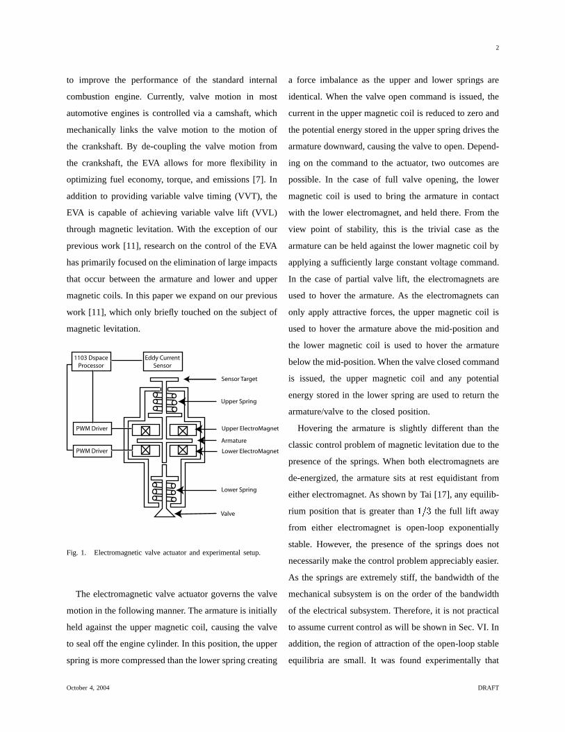
The electromagnetic valve actuator (EVA), shown in
Fig. 1, has recently received attention due to its potential
October 4, 2004 DRAFT
2
to improve the performance of the standard internal
combustion engine. Currently, valve motion in most
automotive engines is controlled via a camshaft, which
mechanically links the valve motion to the motion of
the crankshaft. By de-coupling the valve motion from
the crankshaft, the EVA allows for more flexibility in
optimizing fuel economy, torque, and emissions [7]. In
addition to providing variable valve timing (VVT), the
EVA is capable of achieving variable valve lift (VVL)
through magnetic levitation. With the exception of our
previous work [11], research on the control of the EVA
has primarily focused on the elimination of large impacts
that occur between the armature and lower and upper
magnetic coils. In this paper we expand on our previous
work [11], which only briefly touched on the subject of
magnetic levitation.
PWM Driver
PWM Driver
Eddy Current
Sensor
Sensor Target
1103 Dspace
Processor
Upper Spring
Lower Spring
Armature
Valve
Lower ElectroMagnet
Upper ElectroMagnet
Fig. 1. Electromagnetic valve actuator and experimental setup.
The electromagnetic valve actuator governs the valve
motion in the following manner. The armature is initially
held against the upper magnetic coil, causing the valve
to seal off the engine cylinder. In this position, the upper
spring is more compressed than the lower spring creating
a force imbalance as the upper and lower springs are
identical. When the valve open command is issued, the
current in the upper magnetic coil is reduced to zero and
the potential energy stored in the upper spring drives the
armature downward, causing the valve to open. Depend-
ing on the command to the actuator, two outcomes are
possible. In the case of full valve opening, the lower
magnetic coil is used to bring the armature in contact
with the lower electromagnet, and held there. From the
view point of stability, this is the trivial case as the
armature can be held against the lower magnetic coil by
applying a sufficiently large constant voltage command.
In the case of partial valve lift, the electromagnets are
used to hover the armature. As the electromagnets can
only apply attractive forces, the upper magnetic coil is
used to hover the armature above the mid-position and
the lower magnetic coil is used to hover the armature
below the mid-position. When the valve closed command
is issued, the upper magnetic coil and any potential
energy stored in the lower spring are used to return the
armature/valve to the closed position.
Hovering the armature is slightly different than the
classic control problem of magnetic levitation due to the
presence of the springs. When both electromagnets are
de-energized, the armature sits at rest equidistant from
either electromagnet. As shown by Tai [17], any equilib-
rium position that is greater than ����� the full lift away
from either electromagnet is open-loop exponentially
stable. However, the presence of the springs does not
necessarily make the control problem appreciably easier.
As the springs are extremely stiff, the bandwidth of the
mechanical subsystem is on the order of the bandwidth
of the electrical subsystem. Therefore, it is not practical
to assume current control as will be shown in Sec. VI. In
addition, the region of attraction of the open-loop stable
equilibria are small. It was found experimentally that
October 4, 2004 DRAFT
3
the armature had to start at rest equidistant from both
electromagnets to achieve stable open-loop hovering for
equilibrium positions greater than ����� the full lift away
from either electromagnet. If the armature starts at rest
against the upper magnetic coil, application of the open-
loop equilibrium voltage results in the armature being
brought into contact with the activated electromagnet.
As the latter initial condition is the one experienced
during operation, it is necessary to design a closed-
loop controller to enlarge the region of attraction so
that hovering is achieved for both open-loop stable and
unstable equilibrium positions.
III. MODELING THE ELECTROMAGNETIC VALVE
ACTUATOR
As derived by Wang [19] the dynamics of the EVA
are given by������ � ��� ���� ���� � � ������������ ������������� "!$#%� �'& �)( �'*�'+ ���� � ,.- � �0/ + � !1��2"� �'&� � 3 � � ��4�'+ ���� � ,.- � �5/ + � !$��26��78#.� �'&� � 3 � �9 �84where
�(mm) is the distance from the lower coil, �
(m/s) is the velocity of the armature,+ � (mVs) is the
magnetic flux in the lower coil,+ � (mVs) is the magnetic
flux in the upper coil, (kg) is the combined mass of
the armature and valve,� ������ (N) is the magnetic force
generated by the lower coil,� ����:� (N) is the magnetic
force generated by the upper coil, � (N/mm) is the
spring constant, # (mm) is half the total armature travel,( (kg/s) is the damping coefficient, - � (V) is the voltage
applied to the lower coil, - � (V) is the voltage applied
to the upper coil, and / ( ; ) is the combined resistance
of the wiring and magnetic coil. Numerical values for
all constants are found in Tab. I. Finally, the magnetic
force generated by either coil is given by
� ����� � +=<7�� � 4 (1)
As explained in Sec. II, only one electromagnet is
used to hover the armature. Therefore, without loss of
generality we assume that the lower coil is used and
neglect the dynamics of the upper coil. To simplify
the controller design, new inputs and coordinates are
introduced per
>%? � � � �A@CB> < � � � � @CB> � � + � � +.@CBD � - � � - @CB8Ewhere
� @CB, � @FB , + @CB , and - @CB are the equilibrium position,
velocity, flux, and voltage respectively. The equilibrium
point is now located at the origin, and the system
dynamics are represented in the form� >��� � G ! > & �)HI! > & D (2)
where
G ! > & � JKKKL> < � �9 �?�NM �5OPQ<SR:T �)�� > ? �)( > <9U �VO QXWZY�[R:T �� M O Q:\ R:]_^a` Y$[ ^ OAb_cedR T �fOAb WZY$[ dR T U � �9 �
gihhhjH�! > & � k l �9 �nm8o 4A frequent assumption in the control of electromag-
netic actuators is that the dynamics of the current/flux are
significantly faster than the dynamics of the mechanical
components of the system. This assumption reduces
October 4, 2004 DRAFT
4
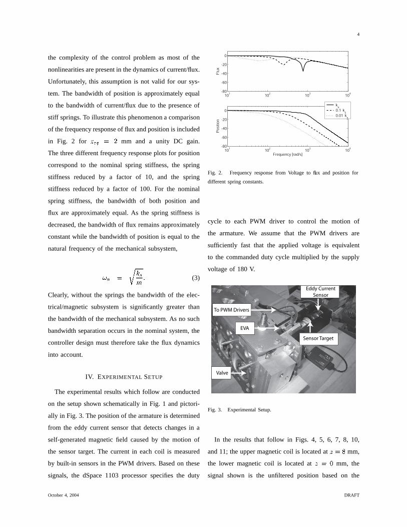
the complexity of the control problem as most of the
nonlinearities are present in the dynamics of current/flux.
Unfortunately, this assumption is not valid for our sys-
tem. The bandwidth of position is approximately equal
to the bandwidth of current/flux due to the presence of
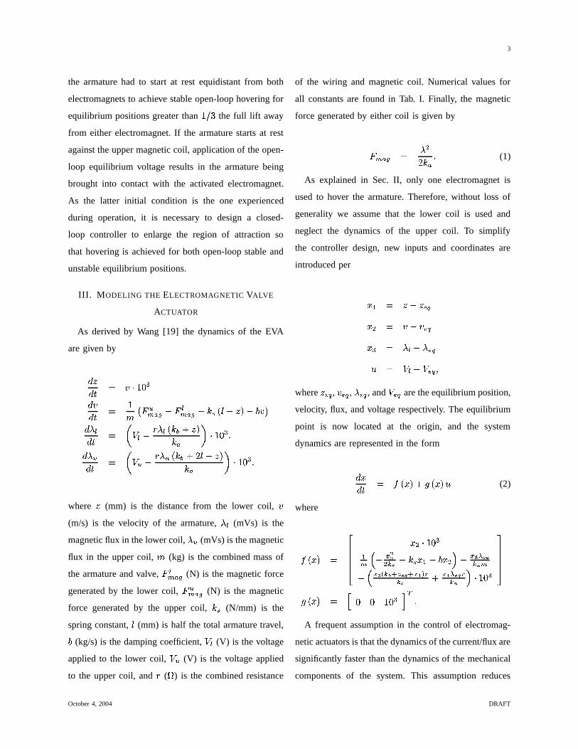
stiff springs. To illustrate this phenomenon a comparison
of the frequency response of flux and position is included
in Fig. 2 for�A@FB � 7 mm and a unity DC gain.
The three different frequency response plots for position
correspond to the nominal spring stiffness, the spring
stiffness reduced by a factor of 10, and the spring
stiffness reduced by a factor of 100. For the nominal
spring stiffness, the bandwidth of both position and
flux are approximately equal. As the spring stiffness is
decreased, the bandwidth of flux remains approximately
constant while the bandwidth of position is equal to the
natural frequency of the mechanical subsystem,
��� � � �� 4 (3)
Clearly, without the springs the bandwidth of the elec-
trical/magnetic subsystem is significantly greater than
the bandwidth of the mechanical subsystem. As no such
bandwidth separation occurs in the nominal system, the
controller design must therefore take the flux dynamics
into account.
IV. EXPERIMENTAL SETUP
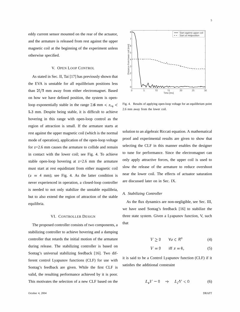
The experimental results which follow are conducted
on the setup shown schematically in Fig. 1 and pictori-
ally in Fig. 3. The position of the armature is determined
from the eddy current sensor that detects changes in a
self-generated magnetic field caused by the motion of
the sensor target. The current in each coil is measured
by built-in sensors in the PWM drivers. Based on these
signals, the dSpace 1103 processor specifies the duty
101
102
103
104
-80
-60
-40
-20
0
Flux
101
102
103
104
-80
-60
-40
-20
0
Frequency [rad/s]
Positio
n
ks
0.1� ks
0.01� ks
Fig. 2. Frequency response from Voltage to flux and position for
different spring constants.
cycle to each PWM driver to control the motion of
the armature. We assume that the PWM drivers are
sufficiently fast that the applied voltage is equivalent
to the commanded duty cycle multiplied by the supply
voltage of 180 V.
Valve
EVA
To PWM Drivers
Eddy Current Sensor
Sensor Target
Fig. 3. Experimental Setup.
In the results that follow in Figs. 4, 5, 6, 7, 8, 10,
and 11; the upper magnetic coil is located at� ��� mm,
the lower magnetic coil is located at� � mm, the
signal shown is the unfiltered position based on the
October 4, 2004 DRAFT
5
eddy current sensor mounted on the rear of the actuator,
and the armature is released from rest against the upper
magnetic coil at the beginning of the experiment unless
otherwise specified.
V. OPEN LOOP CONTROL
As stated in Sec. II, Tai [17] has previously shown that
the EVA is unstable for all equilibrium positions less
than 78# ��� mm away from either electromagnet. Based
on how we have defined position, the system is open-
loop exponentially stable in the range 7 4 � mm � � @CB �� 4 � mm. Despite being stable, it is difficult to achieve
hovering in this range with open-loop control as the
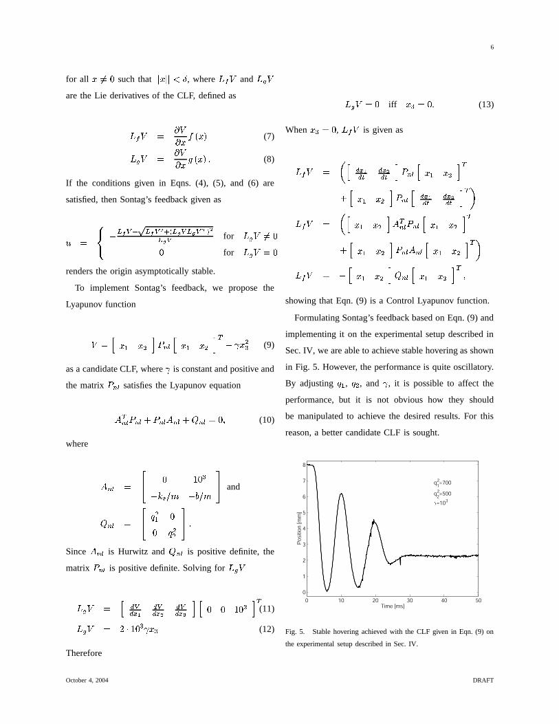
region of attraction is small. If the armature starts at
rest against the upper magnetic coil (which is the normal
mode of operation), application of the open-loop voltage
for z=2.6 mm causes the armature to collide and remain
in contact with the lower coil; see Fig. 4. To achieve
stable open-loop hovering at z=2.6 mm the armature
must start at rest equidistant from either magnetic coil
(� ��� mm); see Fig. 4. As the latter condition is
never experienced in operation, a closed-loop controller
is needed to not only stabilize the unstable equilibria,
but to also extend the region of attraction of the stable
equilibria.
VI. CONTROLLER DESIGN
The proposed controller consists of two components, a
stabilizing controller to achieve hovering and a damping
controller that retards the initial motion of the armature
during release. The stabilizing controller is based on
Sontag’s universal stabilizing feedback [16]. Two dif-
ferent control Lyapunov functions (CLF) for use with
Sontag’s feedback are given. While the first CLF is
valid, the resulting performance achieved by it is poor.
This motivates the selection of a new CLF based on the
0 5 10 15 20 25 30
0
1
2
3
4
5
6
7
8
Dis
tan
ce f
rom
low
er
coil
[mm
]
Time [ms]
Start against upper coilStart at midposition
Fig. 4. Results of applying open-loop voltage for an equilibrium point
2.6 mm away from the lower coil.
solution to an algebraic Riccati equation. A mathematical
proof and experimental results are given to show that
selecting the CLF in this manner enables the designer
to tune for performance. Since the electromagnet can
only apply attractive forces, the upper coil is used to
slow the release of the armature to reduce overshoot
near the lower coil. The effects of actuator saturation
are discussed later on in Sec. IX.
A. Stabilizing Controller
As the flux dynamics are non-negligible, see Sec. III,
we have used Sontag’s feedback [16] to stabilize the
three state system. Given a Lyapunov function, V, such
that
-�� � >�� � (4)-f� iff > � E (5)
it is said to be a Control Lyapunov function (CLF) if it
satisfies the additional constraint
� � -f� ��� - � (6)
October 4, 2004 DRAFT
6
for all >��� such that ��� > ��� ��� , where� � - and
� � -are the Lie derivatives of the CLF, defined as
� � - � � -� > G ! > & (7)
� � - � � -� > HI! > & 4 (8)
If the conditions given in Eqns. (4), (5), and (6) are
satisfied, then Sontag’s feedback given as
D � � ���� �� ^�� �� �� P ^ \ ������������� c P� � � for� � - �� for� � -f�
renders the origin asymptotically stable.
To implement Sontag’s feedback, we propose the
Lyapunov function
-f� k > ? > < m�� � � k > ? > < m8o ��� > <� (9)
as a candidate CLF, where � is constant and positive and
the matrix � � � satisfies the Lyapunov equation
� o� � � � � � � � � � � � �� � � � E (10)
where
� � � � JL � ����� � ��( � gj and
� � � JL"! <? ! <<gj 4
Since� � � is Hurwitz and � � is positive definite, the
matrix � � � is positive definite. Solving for� � -
� � - � k$# �# OAb # �# O P # �# O Q m k l �9 � m o (11)
� � - � 7 � � � � > � (12)
Therefore
� � -f� iff > � � . (13)
When > � � , � � - is given as
� � - � , k # OAb#&% # O P#&% m�� � � k > ? > < m o� k >%? > < m � � � k # O b#&% # O P#&% m o 3� � - � , k > ? > < m � o� � � � � k > ? > < m o� k >%? > < m'� � � � � � k >%? > < m o 3� � - � � k >%? > < m � � k > ? > < m o E
showing that Eqn. (9) is a Control Lyapunov function.
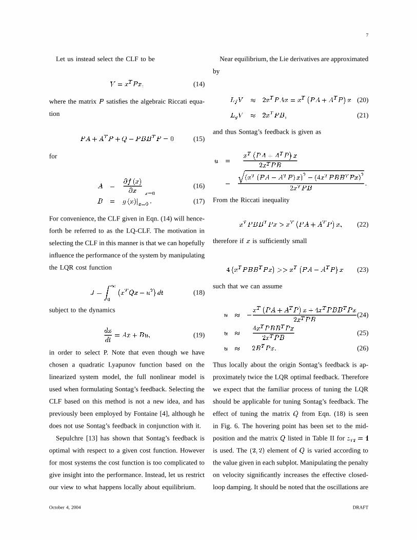
Formulating Sontag’s feedback based on Eqn. (9) and
implementing it on the experimental setup described in
Sec. IV, we are able to achieve stable hovering as shown
in Fig. 5. However, the performance is quite oscillatory.
By adjusting ! ? , ! < , and � , it is possible to affect the
performance, but it is not obvious how they should
be manipulated to achieve the desired results. For this
reason, a better candidate CLF is sought.
0 10 20 30 40 50
0
1
2
3
4
5
6
7
8
Time [ms]
Po
sition
[m
m]
q1=700
2
q2=500
2( =103
Fig. 5. Stable hovering achieved with the CLF given in Eqn. (9) on
the experimental setup described in Sec. IV.
October 4, 2004 DRAFT
7
Let us instead select the CLF to be
-f� > o � > E (14)
where the matrix � satisfies the algebraic Riccati equa-
tion
� � � � o � �� 5� ����� o � � (15)
for
� � � G ! > &� > ���� O�� � (16)
� � H ! > & � O�� � 4 (17)
For convenience, the CLF given in Eqn. (14) will hence-
forth be referred to as the LQ-CLF. The motivation in
selecting the CLF in this manner is that we can hopefully
influence the performance of the system by manipulating
the LQR cost function
� � � �� � > o > � D < * ��� (18)
subject to the dynamics� >��� � � > � � D E (19)
in order to select P. Note that even though we have
chosen a quadratic Lyapunov function based on the
linearized system model, the full nonlinear model is
used when formulating Sontag’s feedback. Selecting the
CLF based on this method is not a new idea, and has
previously been employed by Fontaine [4], although he
does not use Sontag’s feedback in conjunction with it.
Sepulchre [13] has shown that Sontag’s feedback is
optimal with respect to a given cost function. However
for most systems the cost function is too complicated to
give insight into the performance. Instead, let us restrict
our view to what happens locally about equilibrium.
Near equilibrium, the Lie derivatives are approximated
by
��� - 7 > o � � > � > o � � � � � o � * > (20)
� � - 7 > o ��� E (21)
and thus Sontag’s feedback is given as
D � � > o � � � � � o � * >7 > o ���� ! > o ! � � � � o � & > & < � ! � > o ����� o � > & <7 > o ��� 4From the Riccati inequality> o ����� o � > ��> o � � � � � o � * > E (22)
therefore if > is sufficiently small
� � > o ����� o � > * ��� > o � � � � � o � * > (23)
such that we can assume
D � > o � � � � � o � * > � � > o ����� o � >7 > o ��� (24)D � � > o ����� o � >7 > o ��� (25)D ��7 � o � > 4 (26)
Thus locally about the origin Sontag’s feedback is ap-
proximately twice the LQR optimal feedback. Therefore
we expect that the familiar process of tuning the LQR
should be applicable for tuning Sontag’s feedback. The
effect of tuning the matrix from Eqn. (18) is seen
in Fig. 6. The hovering point has been set to the mid-
position and the matrix listed in Table II for��@CB � �
is used. The !$7 E 7 & element of is varied according to
the value given in each subplot. Manipulating the penalty
on velocity significantly increases the effective closed-
loop damping. It should be noted that the oscillations are
October 4, 2004 DRAFT
8
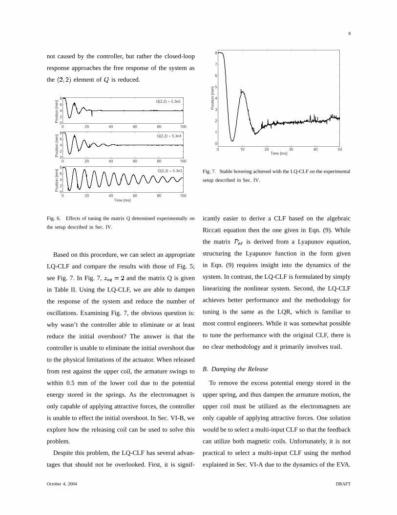
not caused by the controller, but rather the closed-loop
response approaches the free response of the system as
the !�7 E 7 & element of is reduced.
0 20 40 60 80 1000
2
4
6
8
Po
sitio
n [
mm
]
0 20 40 60 80 1000
2
4
6
8
0 20 40 60 80 1000
2
4
6
8
Time [ms]
Q(2,2) = 5.3e5
Q(2,2) = 5.3e4
Q(2,2) = 5.3e3
Po
sitio
n [
mm
]P
ositio
n [
mm
]
Fig. 6. Effects of tuning the matrix Q determined experimentally on
the setup described in Sec. IV.
Based on this procedure, we can select an appropriate
LQ-CLF and compare the results with those of Fig. 5;
see Fig. 7. In Fig. 7,� @CB � 7 and the matrix Q is given
in Table II. Using the LQ-CLF, we are able to dampen
the response of the system and reduce the number of
oscillations. Examining Fig. 7, the obvious question is:
why wasn’t the controller able to eliminate or at least
reduce the initial overshoot? The answer is that the
controller is unable to eliminate the initial overshoot due
to the physical limitations of the actuator. When released
from rest against the upper coil, the armature swings to
within 0.5 mm of the lower coil due to the potential
energy stored in the springs. As the electromagnet is
only capable of applying attractive forces, the controller
is unable to effect the initial overshoot. In Sec. VI-B, we
explore how the releasing coil can be used to solve this
problem.
Despite this problem, the LQ-CLF has several advan-
tages that should not be overlooked. First, it is signif-
0 10 20 30 40 50
0
1
2
3
4
5
6
7
8
Time [ms]
Po
sition
[m
m]
Fig. 7. Stable hovering achieved with the LQ-CLF on the experimental
setup described in Sec. IV.
icantly easier to derive a CLF based on the algebraic
Riccati equation then the one given in Eqn. (9). While
the matrix � � � is derived from a Lyapunov equation,
structuring the Lyapunov function in the form given
in Eqn. (9) requires insight into the dynamics of the
system. In contrast, the LQ-CLF is formulated by simply
linearizing the nonlinear system. Second, the LQ-CLF
achieves better performance and the methodology for
tuning is the same as the LQR, which is familiar to
most control engineers. While it was somewhat possible
to tune the performance with the original CLF, there is
no clear methodology and it primarily involves trail.
B. Damping the Release
To remove the excess potential energy stored in the
upper spring, and thus dampen the armature motion, the
upper coil must be utilized as the electromagnets are
only capable of applying attractive forces. One solution
would be to select a multi-input CLF so that the feedback
can utilize both magnetic coils. Unfortunately, it is not
practical to select a multi-input CLF using the method
explained in Sec. VI-A due to the dynamics of the EVA.
October 4, 2004 DRAFT
9
For equilibria below the mid-position, the effect of the
upper coil on the motion of the armature is lost in the
linearization. This is a result of the fact that the magnetic
force is proportional to the square of the flux and the
equilibrium flux in the upper coil is zero. Therefore the
effect of the upper coil on the motion of the armature
will not be utilized to minimize the penalty on position
and velocity in Eqn. (18).
When hovering, the following methodology is used to
dampen the release of the armature:
1) For both hovering above and below the mid-
position, the voltage across the upper coil is set
to -30 V until the armature has moved 0.1 mm
away from the upper coil.
2) If the equilibrium position is at or above the mid-
position, the closed-loop controller is activated
after the armature has moved 0.1 mm away from
the upper coil.
3) If the equilibrium position is below the mid-
position, the voltage across the upper coil is set to
180 V until the armature is greater than 2 mm away
from the upper coil. After this point, the voltage
across the upper coil is set to zero and the closed-
loop controller is activated. Once the estimated
velocity reaches zero, the flux in the upper coil
is driven to zero with the proportional controller
- � � � � + �since the armature has begun to move away from
the lower coil and thus the upper coil can no longer
effect the overshoot.
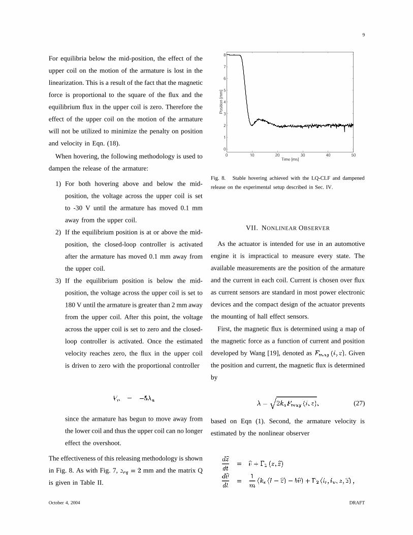
The effectiveness of this releasing methodology is shown
in Fig. 8. As with Fig. 7,� @CB � 7 mm and the matrix Q
is given in Table II.
0 10 20 30 40 50
0
1
2
3
4
5
6
7
8
Time [ms]
Po
sition
[m
m]
Fig. 8. Stable hovering achieved with the LQ-CLF and dampened
release on the experimental setup described in Sec. IV.
VII. NONLINEAR OBSERVER
As the actuator is intended for use in an automotive
engine it is impractical to measure every state. The
available measurements are the position of the armature
and the current in each coil. Current is chosen over flux
as current sensors are standard in most power electronic
devices and the compact design of the actuator prevents
the mounting of hall effect sensors.
First, the magnetic flux is determined using a map of
the magnetic force as a function of current and position
developed by Wang [19], denoted as� ����� !�� E �'& . Given
the position and current, the magnetic flux is determined
by + � 7�� � � ���:� !�� E ��& E (27)
based on Eqn (1). Second, the armature velocity is
estimated by the nonlinear observer������� � � � ��� ? ! � E � ��&��� ���� � � !$� !�#%� ���& �)( � � & ��� < !�� � E � � E � E ���& EOctober 4, 2004 DRAFT
10
where
� ? ! � E � ��& � H ? ! � � ���&� < !�� � E � � E � E � ��& � ���������! � � E �'& � ���������!�� � E �'& � H < ! � � ���& 4Computing the error dynamics, � � JL � � ��� � �� gj , results
in� ���� � JL �9������ � ��( � gj� ��� �
��
� � JL H ?H < gj k � m� �� �
� �
�
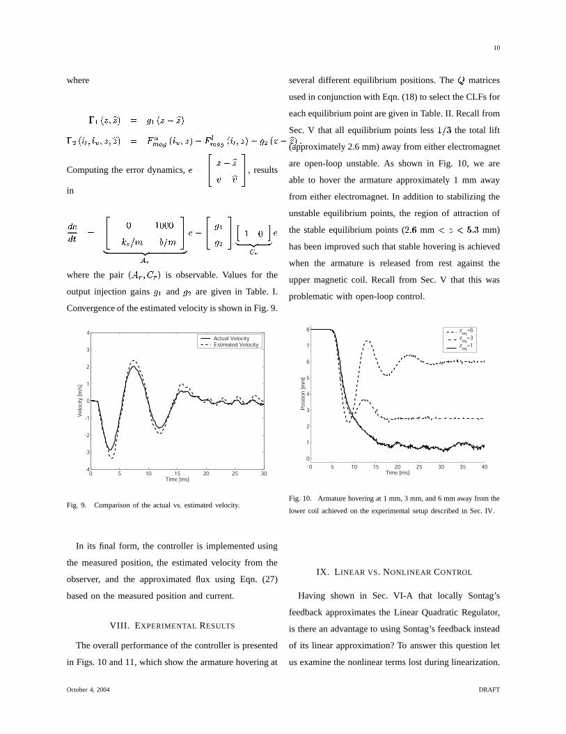
where the pair ! � d E � d & is observable. Values for the
output injection gains H ? and H < are given in Table. I.
Convergence of the estimated velocity is shown in Fig. 9.
0 5 10 15 20 25 30-4
-3
-2
-1
0
1
2
3
4
Velo
city
[m
/s]
Time [ms]
Actual Velocity Estimated Velocity
Fig. 9. Comparison of the actual vs. estimated velocity.
In its final form, the controller is implemented using
the measured position, the estimated velocity from the
observer, and the approximated flux using Eqn. (27)
based on the measured position and current.
VIII. EXPERIMENTAL RESULTS
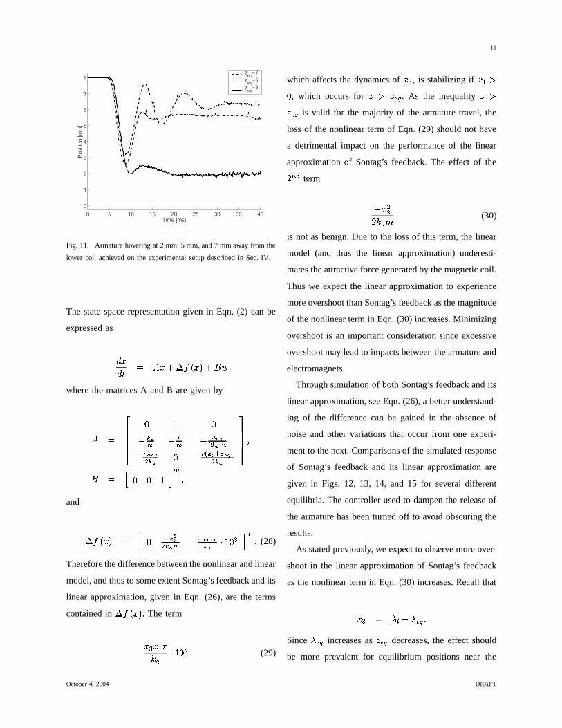
The overall performance of the controller is presented
in Figs. 10 and 11, which show the armature hovering at
several different equilibrium positions. The matrices
used in conjunction with Eqn. (18) to select the CLFs for
each equilibrium point are given in Table. II. Recall from
Sec. V that all equilibrium points less � � � the total lift
(approximately 2.6 mm) away from either electromagnet
are open-loop unstable. As shown in Fig. 10, we are
able to hover the armature approximately 1 mm away
from either electromagnet. In addition to stabilizing the
unstable equilibrium points, the region of attraction of
the stable equilibrium points ( 7 4 � mm � � � � 4 � mm)
has been improved such that stable hovering is achieved
when the armature is released from rest against the
upper magnetic coil. Recall from Sec. V that this was
problematic with open-loop control.
0 5 10 15 20 25 30 35 40
0
1
2
3
4
5
6
7
8
Time [ms]
Po
sition
[m
m]
zeq=6
zeq=3
zeq=1
Fig. 10. Armature hovering at 1 mm, 3 mm, and 6 mm away from the
lower coil achieved on the experimental setup described in Sec. IV.
IX. LINEAR VS. NONLINEAR CONTROL
Having shown in Sec. VI-A that locally Sontag’s
feedback approximates the Linear Quadratic Regulator,
is there an advantage to using Sontag’s feedback instead
of its linear approximation? To answer this question let
us examine the nonlinear terms lost during linearization.
October 4, 2004 DRAFT
11
0 5 10 15 20 25 30 35 40
0
1
2
3
4
5
6
7
8
Time [ms]
Po
sition
[m
m]
zeq=7
zeq=5
zeq=2
Fig. 11. Armature hovering at 2 mm, 5 mm, and 7 mm away from the
lower coil achieved on the experimental setup described in Sec. IV.
The state space representation given in Eqn. (2) can be
expressed as � >��� � � > ��� G ! > & � � Dwhere the matrices A and B are given by
� � JKKKL � � R��� � 2� � WZY�[<SR:T �� d WZY�[<�R:T � d \ R:]_^a` Y$[ c<�R:Tgihhhj E
� � k � m o Eand
� G ! > & � k � OPQ<SR T � � O Q O b dR T � � � m8o 4 (28)
Therefore the difference between the nonlinear and linear
model, and thus to some extent Sontag’s feedback and its
linear approximation, given in Eqn. (26), are the terms
contained in � G ! > & . The term
� > � >%? /� � � �9 � (29)
which affects the dynamics of > � , is stabilizing if > ? � , which occurs for� � � @CB
. As the inequality� �� @CB
is valid for the majority of the armature travel, the
loss of the nonlinear term of Eqn. (29) should not have
a detrimental impact on the performance of the linear
approximation of Sontag’s feedback. The effect of the7 � # term
� > <�7�� � (30)
is not as benign. Due to the loss of this term, the linear
model (and thus the linear approximation) underesti-
mates the attractive force generated by the magnetic coil.
Thus we expect the linear approximation to experience
more overshoot than Sontag’s feedback as the magnitude
of the nonlinear term in Eqn. (30) increases. Minimizing
overshoot is an important consideration since excessive
overshoot may lead to impacts between the armature and
electromagnets.
Through simulation of both Sontag’s feedback and its
linear approximation, see Eqn. (26), a better understand-
ing of the difference can be gained in the absence of
noise and other variations that occur from one experi-
ment to the next. Comparisons of the simulated response
of Sontag’s feedback and its linear approximation are
given in Figs. 12, 13, 14, and 15 for several different
equilibria. The controller used to dampen the release of
the armature has been turned off to avoid obscuring the
results.
As stated previously, we expect to observe more over-
shoot in the linear approximation of Sontag’s feedback
as the nonlinear term in Eqn. (30) increases. Recall that
> � � + � � + @CB 4Since
+ @CBincreases as
� @CBdecreases, the effect should
be more prevalent for equilibrium positions near the
October 4, 2004 DRAFT
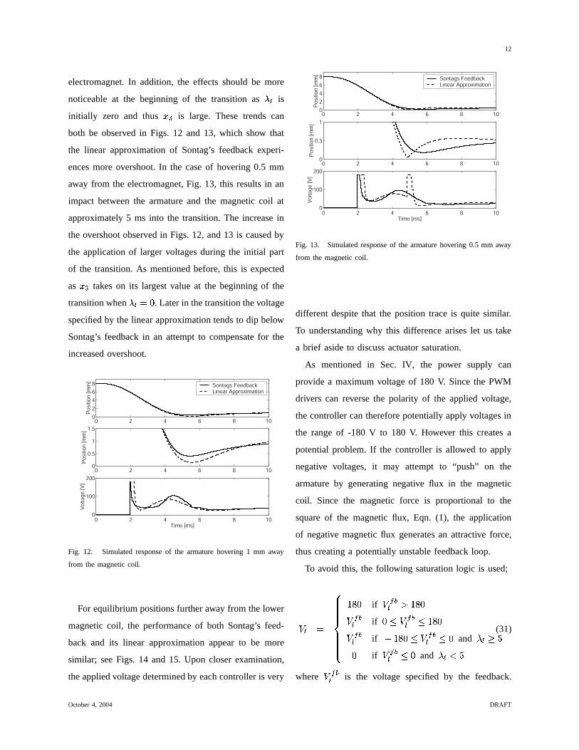
12
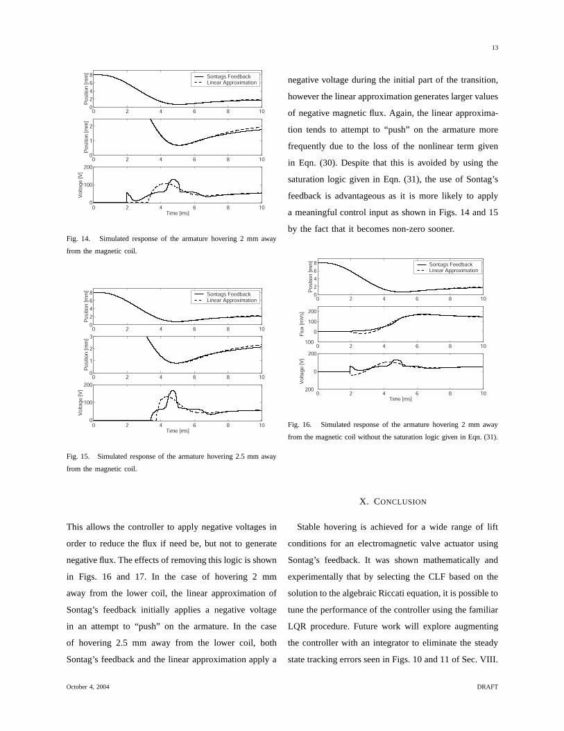
electromagnet. In addition, the effects should be more
noticeable at the beginning of the transition as+ � is
initially zero and thus > � is large. These trends can
both be observed in Figs. 12 and 13, which show that
the linear approximation of Sontag’s feedback experi-
ences more overshoot. In the case of hovering 0.5 mm
away from the electromagnet, Fig. 13, this results in an
impact between the armature and the magnetic coil at
approximately 5 ms into the transition. The increase in
the overshoot observed in Figs. 12, and 13 is caused by
the application of larger voltages during the initial part
of the transition. As mentioned before, this is expected
as > � takes on its largest value at the beginning of the
transition when+ � � . Later in the transition the voltage
specified by the linear approximation tends to dip below
Sontag’s feedback in an attempt to compensate for the
increased overshoot.
0 2 4 6 8 100
2
4
6
8
Po
sitio
n [
mm
]
Sontags Feedback Linear Approximation
0 2 4 6 8 100
0.5
1
1.5
Po
sitio
n [
mm
]
0 2 4 6 8 100
100
200
Volta
ge
[V
]
Time [ms]
Fig. 12. Simulated response of the armature hovering 1 mm away
from the magnetic coil.
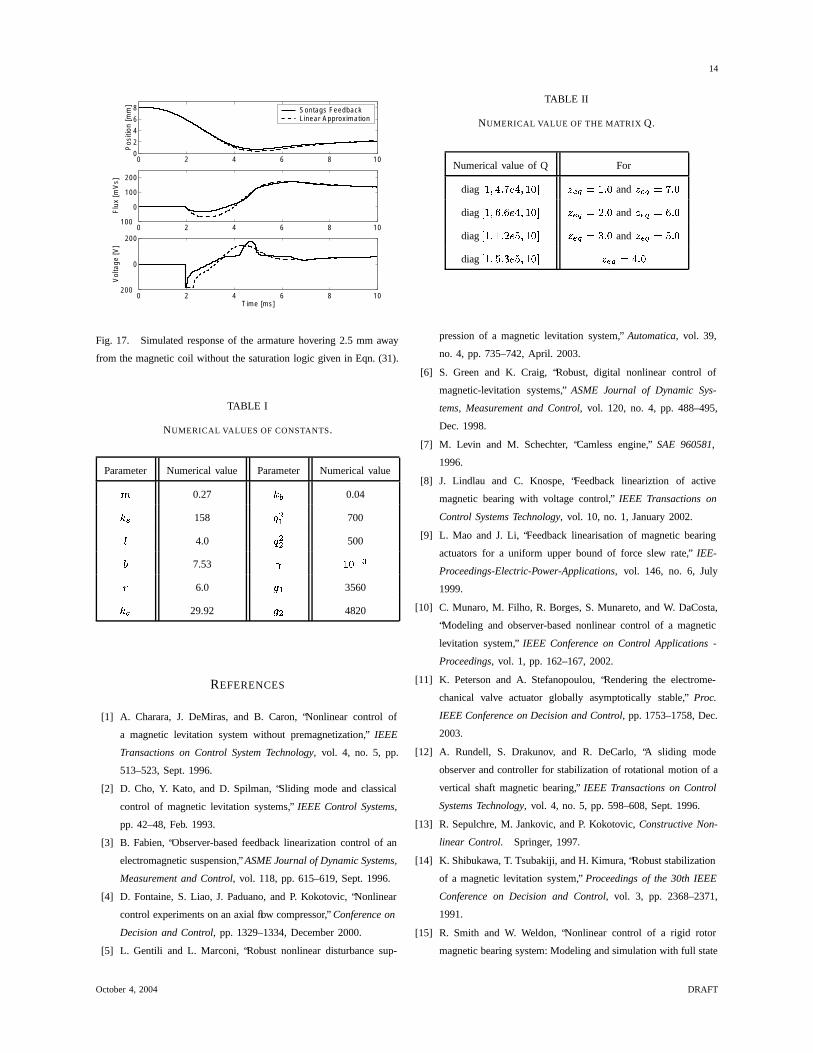
For equilibrium positions further away from the lower
magnetic coil, the performance of both Sontag’s feed-
back and its linear approximation appear to be more
similar; see Figs. 14 and 15. Upon closer examination,
the applied voltage determined by each controller is very
0 2 4 6 8 100
2
4
6
8
Po
sitio
n [
mm
]
Sontags Feedback Linear Approximation
0 2 4 6 8 100
0.5
1
Po
sitio
n [
mm
]
0 2 4 6 8 100
100
200
Volta
ge
[V
]
Time [ms]
Fig. 13. Simulated response of the armature hovering 0.5 mm away
from the magnetic coil.
different despite that the position trace is quite similar.
To understanding why this difference arises let us take
a brief aside to discuss actuator saturation.
As mentioned in Sec. IV, the power supply can
provide a maximum voltage of 180 V. Since the PWM
drivers can reverse the polarity of the applied voltage,
the controller can therefore potentially apply voltages in
the range of -180 V to 180 V. However this creates a
potential problem. If the controller is allowed to apply
negative voltages, it may attempt to “push” on the
armature by generating negative flux in the magnetic
coil. Since the magnetic force is proportional to the
square of the magnetic flux, Eqn. (1), the application
of negative magnetic flux generates an attractive force,
thus creating a potentially unstable feedback loop.
To avoid this, the following saturation logic is used;
- � ��������������
� � if - � 2� � � � - � 2� if � - � 2� � � � - � 2� if � � � � - � 2� � and+ � � � if - � 2� � and
+ � � � (31)
where - � 2� is the voltage specified by the feedback.
October 4, 2004 DRAFT
13
0 2 4 6 8 100
2
4
6
8
Po
sitio
n [
mm
]
Sontags Feedback Linear Approximation
0 2 4 6 8 100
1
2
Po
sitio
n [
mm
]
0 2 4 6 8 100
100
200
Volta
ge
[V
]
Time [ms]
Fig. 14. Simulated response of the armature hovering 2 mm away
from the magnetic coil.
0 2 4 6 8 100
2
4
6
8
Po
sitio
n [
mm
]
Sontags Feedback Linear Approximation
0 2 4 6 8 100
1
2
3
Po
sitio
n [
mm
]
0 2 4 6 8 100
100
200
Volta
ge
[V
]
Time [ms]
Fig. 15. Simulated response of the armature hovering 2.5 mm away
from the magnetic coil.
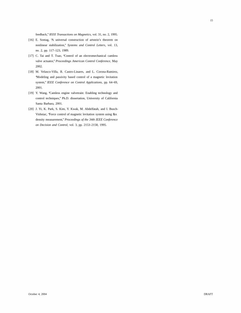
This allows the controller to apply negative voltages in
order to reduce the flux if need be, but not to generate
negative flux. The effects of removing this logic is shown
in Figs. 16 and 17. In the case of hovering 2 mm
away from the lower coil, the linear approximation of
Sontag’s feedback initially applies a negative voltage
in an attempt to “push” on the armature. In the case
of hovering 2.5 mm away from the lower coil, both
Sontag’s feedback and the linear approximation apply a
negative voltage during the initial part of the transition,
however the linear approximation generates larger values
of negative magnetic flux. Again, the linear approxima-
tion tends to attempt to “push” on the armature more
frequently due to the loss of the nonlinear term given
in Eqn. (30). Despite that this is avoided by using the
saturation logic given in Eqn. (31), the use of Sontag’s
feedback is advantageous as it is more likely to apply
a meaningful control input as shown in Figs. 14 and 15
by the fact that it becomes non-zero sooner.
0 2 4 6 8 100
2
4
6
8
Posi
tion [m
m]
Sontags Feedback Linear Approximation
0 2 4 6 8 10100
0
100
200
Flux
[mV
s]
0 2 4 6 8 10200
0
200
Volta
ge [V
]
Time [ms]
Fig. 16. Simulated response of the armature hovering 2 mm away
from the magnetic coil without the saturation logic given in Eqn. (31).
X. CONCLUSION
Stable hovering is achieved for a wide range of lift
conditions for an electromagnetic valve actuator using
Sontag’s feedback. It was shown mathematically and
experimentally that by selecting the CLF based on the
solution to the algebraic Riccati equation, it is possible to
tune the performance of the controller using the familiar
LQR procedure. Future work will explore augmenting
the controller with an integrator to eliminate the steady
state tracking errors seen in Figs. 10 and 11 of Sec. VIII.
October 4, 2004 DRAFT
14
0 2 4 6 8 100
2
4
6
8
Pos
ition
[mm
]
Sontags Feedback Linear Approximation
0 2 4 6 8 10100
0
100
200
Flu
x [m
Vs]
0 2 4 6 8 10200
0
200
Vol
tage
[V]
Time [ms]
Fig. 17. Simulated response of the armature hovering 2.5 mm away
from the magnetic coil without the saturation logic given in Eqn. (31).
TABLE I
NUMERICAL VALUES OF CONSTANTS.
Parameter Numerical value Parameter Numerical value
� 0.27���
0.04
���158 ���� 700
4.0 � �� 500
7.53 � �� ����
� 6.0 � � 3560
���29.92 � � 4820
REFERENCES
[1] A. Charara, J. DeMiras, and B. Caron, “Nonlinear control of
a magnetic levitation system without premagnetization,” IEEE
Transactions on Control System Technology, vol. 4, no. 5, pp.
513–523, Sept. 1996.
[2] D. Cho, Y. Kato, and D. Spilman, “Sliding mode and classical
control of magnetic levitation systems,” IEEE Control Systems,
pp. 42–48, Feb. 1993.
[3] B. Fabien, “Observer-based feedback linearization control of an
electromagnetic suspension,” ASME Journal of Dynamic Systems,
Measurement and Control, vol. 118, pp. 615–619, Sept. 1996.
[4] D. Fontaine, S. Liao, J. Paduano, and P. Kokotovic, “Nonlinear
control experiments on an axial flow compressor,” Conference on
Decision and Control, pp. 1329–1334, December 2000.
[5] L. Gentili and L. Marconi, “Robust nonlinear disturbance sup-
TABLE II
NUMERICAL VALUE OF THE MATRIX Q.
Numerical value of Q For
diag � ������� ��� ���!�� #" $#%'&)(*��� and $#%�&)(+��� diag � ���',�� ,�� ���!�� #" $ %'& (.-�� and $ %�& (.,�� diag � ������� -��#/��!�� #" $ %'& (.0�� and $ %�& (./�� diag � ���'/�� 0��#/��!�� #" $ %'& (1���
pression of a magnetic levitation system,” Automatica, vol. 39,
no. 4, pp. 735–742, April. 2003.
[6] S. Green and K. Craig, “Robust, digital nonlinear control of
magnetic-levitation systems,” ASME Journal of Dynamic Sys-
tems, Measurement and Control, vol. 120, no. 4, pp. 488–495,
Dec. 1998.
[7] M. Levin and M. Schechter, “Camless engine,” SAE 960581,
1996.
[8] J. Lindlau and C. Knospe, “Feedback lineariztion of active
magnetic bearing with voltage control,” IEEE Transactions on
Control Systems Technology, vol. 10, no. 1, January 2002.
[9] L. Mao and J. Li, “Feedback linearisation of magnetic bearing
actuators for a uniform upper bound of force slew rate,” IEE-
Proceedings-Electric-Power-Applications, vol. 146, no. 6, July
1999.
[10] C. Munaro, M. Filho, R. Borges, S. Munareto, and W. DaCosta,
“Modeling and observer-based nonlinear control of a magnetic
levitation system,” IEEE Conference on Control Applications -
Proceedings, vol. 1, pp. 162–167, 2002.
[11] K. Peterson and A. Stefanopoulou, “Rendering the electrome-
chanical valve actuator globally asymptotically stable,” Proc.
IEEE Conference on Decision and Control, pp. 1753–1758, Dec.
2003.
[12] A. Rundell, S. Drakunov, and R. DeCarlo, “A sliding mode
observer and controller for stabilization of rotational motion of a
vertical shaft magnetic bearing,” IEEE Transactions on Control
Systems Technology, vol. 4, no. 5, pp. 598–608, Sept. 1996.
[13] R. Sepulchre, M. Jankovic, and P. Kokotovic, Constructive Non-
linear Control. Springer, 1997.
[14] K. Shibukawa, T. Tsubakiji, and H. Kimura, “Robust stabilization
of a magnetic levitation system,” Proceedings of the 30th IEEE
Conference on Decision and Control, vol. 3, pp. 2368–2371,
1991.
[15] R. Smith and W. Weldon, “Nonlinear control of a rigid rotor
magnetic bearing system: Modeling and simulation with full state
October 4, 2004 DRAFT
15
feedback,” IEEE Transactions on Magnetics, vol. 31, no. 2, 1995.
[16] E. Sontag, “A universal construction of artstein’s theorem on
nonlinear stabilization,” Systems and Control Letters, vol. 13,
no. 2, pp. 117–123, 1989.
[17] C. Tai and T. Tsao, “Control of an electromechanical camless
valve actuator,” Proceedings American Control Conference, May
2002.
[18] M. Velasco-Villa, R. Castro-Linares, and L. Corona-Ramirez,
“Modeling and passivity based control of a magnetic levitation
system,” IEEE Conference on Control Applications, pp. 64–69,
2001.
[19] Y. Wang, “Camless engine valvetrain: Enabling technology and
control techniques,” Ph.D. dissertation, University of California
Santa Barbara, 2001.
[20] J. Yi, K. Park, S. Kim, Y. Kwak, M. Abdelfatah, and I. Busch-
Vishniac, “Force control of magnetic levitation system using flux
density measurement,” Proceedings of the 34th IEEE Conference
on Decision and Control, vol. 3, pp. 2153–2158, 1995.
October 4, 2004 DRAFT