NONLINEAR CONTROLLABILITY OF SINGULARLY PERTURBED

International Journal of Pure and Applied Mathematics————————————————————————–Volume 47 No. 2 2008, 243-266

NONLINEAR CONTROLLABILITY OF SINGULARLY

PERTURBED MODELS OF POWER FLOW NETWORKS

Steven Ball1, Ernest Barany2, Steve Schaffer3, Kevin Wedeward4 §

1Science Applications International CorporationColumbia, MD, USA

email: [email protected] of Mathematical Sciences

New Mexico State UniversityLas Cruces, NM, USA

email: [email protected] of Mathematics

New Mexico Institute of Mining and TechnologySocorro, NM, USA

email: [email protected] of Electrical Engineering

New Mexico Institute of Mining and Technology801 Leroy Place, Socorro, NM 87801, USA

email: [email protected]

Abstract: A method based on differential geometric control theory is pre-sented to provide insight into how nodes (busses) of a power network affect eachother. The network model considered is derived from a singular perturbationof the standard power flow equations. Accessibility properties of the model areinvestigated, and it is shown that a network with chain topology is feedbacklinearizable. This result is illustrated through computer simulation and controlof an example network. The findings are extended to input-output lineariza-tion of large power networks where full feedback linearization is not feasible.Simulation results are shown for control across an IEEE test system with 118busses.

AMS Subject Classification: 93B05, 93B52, 58E25Key Words: power networks, accessibility, feedback linearization, control

Received: June 11, 2008 c© 2008, Academic Publications Ltd.

§Correspondence author

244 S. Ball, E. Barany, S. Schaffer, K. Wedeward

1. Introduction

Dynamic analysis of large electric power networks is increasingly important aspower systems become larger and more interconnected, and are operated closerto stability limits. Power networks are high dimensional dynamic systems com-posed of heterogeneous components governed by nonlinear evolution equationsand subject to disturbances. These facts make them particularly difficult toanalyze and the focus of much attention (see, e.g., [3, 4, 5, 10]). An importantaspect of the dynamic behavior of power systems that is particularly difficultto codify is that directly related to network structure. The connectivity impliesthat any change at one bus necessarily affects all busses, so that fundamentalquestions such as how power from a given bus is distributed in the network arequite subtle.

Power networks can be represented as planar graphs, which are much-studied objects, however being neither regular nor random they fall into acategory that is somewhat resistant to conventional approaches, see [14]. Powergrids are typically modeled mesoscopically, meaning that they generally con-sist of tens to thousands of nodes, and their dynamics take place in a statespace with two to perhaps twenty dimensions per node. In this paper geo-metric control theory is used to analyze the network-dependent structure ofpower systems. This paper begins the investigation by considering perhaps thesimplest dynamics possible based on conventional power flow equations. Mini-mally complicated dynamic models of power networks are constructed as affinenonlinear control systems and used to investigate how inputs of a given nodeinfluence the other nodes. This question is of enormous importance for thestudy of stability, and also has direct economic implications in regard to how agiven generator-load pair interact.

2. Dynamic Models of Power Networks

An electric power network can be usefully modeled in the context of what areknown as “coupled cell” systems in the nonlinear dynamics and control lit-erature. The cells correspond to busses (nodes) of the power networks, anddevices connected to the busses such as generators, loads, voltage control de-vices or other components define internal states and dynamics of the cells. Acharacteristic of power networks that simplifies this analysis is when the cou-pling between nodes occurs solely through the power flow equations. This is

NONLINEAR CONTROLLABILITY OF SINGULARLY... 245

not always strictly true as certain devices such as transformers and static VARcompensators are located between busses, but these devices can often be ab-sorbed into redefinitions of effective busses and lines. In this case the evolutionof the internal states of the devices sees only the voltage phasor of the bus towhich it is connected, and also that the evolution of the voltage phasor dependsonly on the bus’s own internal states and the voltages of the other busses towhich it is connected (but not the internal states of those busses).

The nature of the evolutionary equations depends on the modeling paradigm.The simplest representation of an operating power grid is its power flow (loadflow) solution, see [5, 10]. In this situation real and reactive power generationand consumption are regarded as constant, and the solution is a set of constantvoltage phasors for the nodes. In this context there are no dynamics at all.Adding internal node dynamics to this picture results in a differential-algebraicsystem of equations (DAE) in which case the equations for the j-th node of thenetwork take the form

zj = fj(zj ,Vj) , (1)

0 = Pj + iQj − ΣkVjVkYjk , (2)

where zj is the vector of internal states, Vj is the voltage phasor, Pj and Qj

are the real and reactive power injection at the node which can be positive ornegative and may depend on internal states and the voltage phasor [5, 10]. Yjk

is the admittance of the line connecting node j to node k, which vanishes if thetwo nodes are not directly connected.

The assumption of exact solution of the power flow equations (2) for alltimes is an approximation that amounts to regarding the dynamics at the busas infinitely fast. This can be a convenient assumption, but is not really justifiedfrom first principles. In fact, there will be nontrivial dynamics on fast, but finite,time scales that depend in a complicated way on the specifics of the devicesconnected to the bus. The infinitely fast dynamics of the power flow equationsis often justified by arguing that no realistic modeling of the fast dynamics ispossible in general. While this may be so, there is another solution seen in theliterature [3, 5, 8, 9, 12, 2] that has its own advantages, which is to replaceequation (2) with a singularly perturbed version (SPDE) that reflects that thevoltage phasor will exhibit fast dynamics. This type of approximation cannotbe used thoughtlessly (see, e.g., Chapter 8 of [5]), but sufficiently close to ahyperbolic fixed point there is reason to believe that smooth fast dynamicsexist, and a perturbation of this type can be very useful.

The precise way in which the time evolution of the phasor components is as-sociated with the mismatch of power flow is not uniquely determined. However,


in some common situations (see [3, 5, 8]) the lore of the electrical engineeringliterature attributes evolution of the phasor angle to the real power mismatch,and that of the voltage amplitude to the reactive power mismatch. In this case,the (fully dynamic) equations for the j th node become

zj = fj(zj ,Vj) , (3)

ǫθj = Pj − Re(ΣkVjVkYjk) , (4)

ǫVj = Qj − Im(ΣkVjVkYjk) , (5)

where ǫ ≪ 1 is a representation of the separation of fast and slow time scales.

The equations (3)-(5) have many advantages over equations (1)-(2) fromthe point of view of analysis and simulation. Simulations of DAEs can behampered by the need to find good initial conditions which also affects theability of such simulations to deal with protection events such as load sheddingor line and generator tripping. Also, being a smooth dynamic system the toolsof nonlinear dynamics such as bifurcation theory and Lyapunov stability can beapplied more easily. Finally, as will be seen below, the methods of differentialgeometric control theory can be easily adapted to provide a means of lookingat the node influence problem that is the heart of this paper.

It should be acknowledged that the nonuniqueness of the association ofthe evolution of states to the power mismatch is somewhat problematic froma modeling point of view. Mathematically, however, one can think in termsof “blowups” of singular problems in the sense of Takens [11]. This theoryguarantees that when the techniques are valid (i.e., away from singularities ofthe DAE, see [5]) and properly interpreted any such desingularization can beused to provide information about the associated DAE. Experience with thesemodels seems to support these ideas, and we take the position that any stableblowup of the DAE is an equally good representative of the fast dynamics as faras the large scale, long time structure of the network is concerned. Moreover, inthe differential geometric context to be laid out below, many considerations areinvariant under diffeomorphism, so that a wide class of possible desingulariza-tions are equivalent. In fact, the controllability results presented below are in away independent of this choice, though the details of the dynamic trajectoriescertainly depend on it.

3. Affine Control Model of Power Flow Networks

The coupled cell structure allows the full control problem to be addressed intwo stages. The fundamental quantities at each bus can be taken to be the


real and reactive powers, which are functions of the bus states (i.e., the voltagephasors) and the internal states. The separation of internal bus states fromgrid states suggests the strategy of using the power injections at each bus ascontrols at the network level, and later taking up the problem of tracking thedesired powers by manipulating the inputs of the internal systems. In otherwords, the assumption is that components of the power at the control bus canbe directly manipulated as inputs.

In practice, the reasoning in the preceding paragraph allows us to ignore thepresence of the internal states. We regard the powers either as parameters orcontrols, depending on the role of the bus. The starting point of the simulationis a power flow solution obtained using standard Newton-Raphson techniques.For computational and analytic reasons rectangular coordinates are adoptedfor the complex phasors Vj = xj + iyj . The more familiar polar form will beused in the larger example that concludes the paper. In the rectangular casethe power flow equations depend only on two types of quadratic polynomials.For notational simplicity, we define

Djk = xjxk + yjyk ,

Cjk = xjyk − xkyj ,

and the equations we consider are

xj = Pj + Σk(DjkGjk − CjkBjk) , (6)

yj = Qj − Σk(DjkBjk + CjkGjk) , (7)

where Gjk is the real part of Yjk (the conductance) and Bjk is the imaginarypart (the susceptance). We have absorbed the singular parameter ǫ into thedefinition of the unit of time which is permissible at this stage since we areassuming no internal (slow time) dynamics are present. As mentioned above,the power components Pj and Qj , j = 1, 2, . . . , N are either parameters orcontrols as described below.

To construct the affine control system, we assume that we have control ofthe inputs at some bus, which we label as node 1. That is, we identify P1 and Q1

as control inputs. Denoting by x the state vector constructed by concatenatingall n = 2N phasor components, where N is the number of busses, the resultingcontrol system is

x = f(x) + g1uP + g2uQ , (8)

where g1 = (1, 0, 0, . . . , 0)T and g2 = (0, 1, 0, . . . , 0)T are the control vectorfields associated with the inputs uP and uQ which are the departures of thepower inputs from their equilibrium values. f(x) is the rest of equations (6)and (7) after the control vectors have been isolated and is referred to as the


drift of the affine control system.

Putting the system into this form allows us to address the question of howmanipulating the inputs to node 1 can affect the state of the system. We use theapparatus of differential geometric control [6, 7, 13]. The problem we consideris a type of input-output control. Specifically, we wish to find control laws forthe power inputs at bus 1 that will steer the voltage phasor at another busto prescribed values. We will achieve this by the technique of input-outputlinearization.

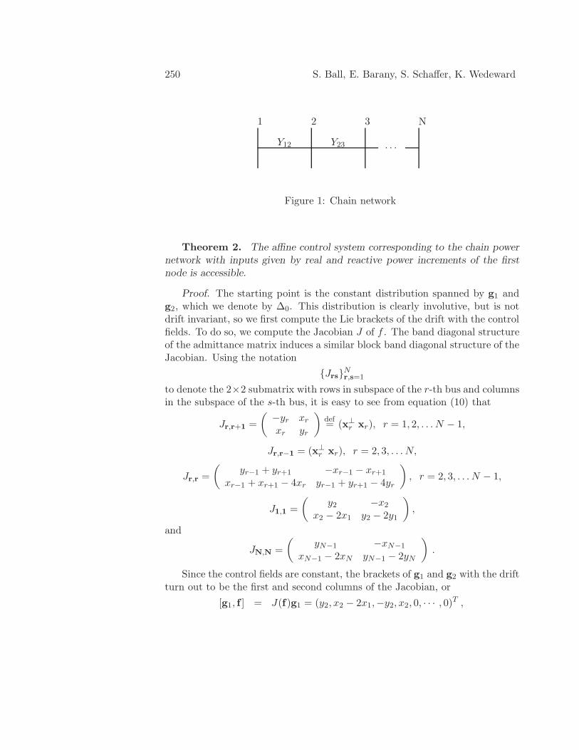
As the starting point of the analysis we consider the simple example of anetwork with chain topology of length N and consider manipulating the inputsat the endpoint (see Figure 1). It will be seen that this network is particularlywell suited to these methods, and that for arbitrary networks, the input-outputgoal is achieved by identifying the chain as the shortest path in a connectednetwork that links the control bus to the output bus. This will be discussedfurther below.

4. Accessibility Properties

To begin, we define the fundamental object of study.

Definition 1. The node accessibility algebra of node 1 is the smallestinvolutive, drift invariant distribution that contains the control vector fields g1

and g2. Note that this distribution comprises a Lie algebra.

A fundamental result from differential geometric control theory is that ifthe dimension of this distribution is d, then the system of equation (8) can bediffeomorphically put into triangular form in a neighborhood of a regular point x

such that an n−d dimensional subspace is uncontrolled, and the reachable set ofthe control system contains an open subset of the complementary d dimensionalsubspace. The corollary is that when the distribution has full rank, the system’sreachable set is an open subset of the state space. This is a necessary conditionfor controllability.

The simplifying feature of the chain topology is that the admittance matrixis band diagonal consisting of the main diagonal and the first super- and sub-diagonals. For simplicity, we assume the conductance Gjk vanishes for all links(which amounts to assuming lossless) and that the susceptance is the same forall links Bjk = − 1

Xwhich implies Bjj = nj

1X

, where nj is the number of nodesconnected to node j, see [10]. It is easy to see that the controllability results


are independent of these assumptions.

The system can be written

x1 = P1 +1

XC12 ,

y1 = Q1 +1

X(D12 − D11) ,

x2 = P2 +1

X(C21 + C23) ,

y2 = Q2 +1

X(D21 + D23 − 2D22) ,

...

xj = Pj +1

X(Cj,j−1 + Cj,j+1) , (9)

yj = Qj +1

X(Dj,j−1 + Dj,j+1 − 2Djj) ,

...

xN = PN +1

XCN,N−1 ,

yN = QN +1

X(DN,N−1 − DNN ) .

By a further rescaling of time, and defining Pj = XPj , we can eliminatethe constant X from the equations and we have a system of the form shown inequation (8) where

f =

P1 + C12

Q1 + D12 − D11

P2 + C21 + C23

Q2 + D21 + D23 − 2D22...

Pj + Cj,j−1 + Cj,j+1

Qj + Dj,j−1 + Dj,j+1 − 2Djj

...

PN + CN,N−1

Qj + DN,N−1 − DNN

(10)

and, where g1 and g2 are defined as above.

We proceed to compute the node accessibility algebra. Specifically, weprove:


· · ·

1 2 3 N

Y12 Y23

Figure 1: Chain network

Theorem 2. The affine control system corresponding to the chain powernetwork with inputs given by real and reactive power increments of the firstnode is accessible.

Proof. The starting point is the constant distribution spanned by g1 andg2, which we denote by ∆0. This distribution is clearly involutive, but is notdrift invariant, so we first compute the Lie brackets of the drift with the controlfields. To do so, we compute the Jacobian J of f . The band diagonal structureof the admittance matrix induces a similar block band diagonal structure of theJacobian. Using the notation

{Jrs}Nr,s=1

to denote the 2×2 submatrix with rows in subspace of the r-th bus and columnsin the subspace of the s-th bus, it is easy to see from equation (10) that

Jr,r+1 =

(

−yr xr

xr yr

)

def= (x⊥

r xr), r = 1, 2, . . . N − 1,

Jr,r−1 = (x⊥r xr), r = 2, 3, . . . N,

Jr,r =

(

yr−1 + yr+1 −xr−1 − xr+1

xr−1 + xr+1 − 4xr yr−1 + yr+1 − 4yr

)

, r = 2, 3, . . . N − 1,

J1,1 =

(

y2 −x2

x2 − 2x1 y2 − 2y1

)

,

and

JN,N =

(

yN−1 −xN−1

xN−1 − 2xN yN−1 − 2yN

)

.

Since the control fields are constant, the brackets of g1 and g2 with the driftturn out to be the first and second columns of the Jacobian, or

[g1, f ] = J(f)g1 = (y2, x2 − 2x1,−y2, x2, 0, · · · , 0)T ,


[g2, f ] = J(f)g2 = (−x2, y2 − 2y1, x2, y2, 0, · · · , 0)T .

To simplify the subsequent analysis, we do not take these fields as generatorsof the accessibility algebra, but instead use g1 and g2 to simplify the fields byeliminating the components in the subspace of bus 1. Therefore, we take as ournew distribution

∆1 = ∆0 ⊕ span{g3,g4} ,

where

g3 = (0, 0,−y2, x2, 0, · · · , 0)T ,

g4 = (0, 0, x2, y2, 0, · · · , 0)T ,

or, using the block index notation

(g3)r = x⊥2 δr2 ,

(g4)r = x2δr2 .

The important observation here is that since detJ21 = |x2|2 these new fields

span the state space for bus 2 as long as the voltage there does not vanish. Soby allowing our direct controls to interact with the drift, we extend our abilityto influence the system by a distance of one connection.

Now, ∆1 is again involutive but is not drift invariant, so we continue theprocedure by computing the brackets of g3 and g4 with the drift. Since thesenew vector fields are state dependent, we must consider both terms in thebracket. For example, for g3, we have

[g3, f ] = J(f)g3 − J(g3)f .

The second term is irrelevant for purposes of accessibility since it always lies inthe subspace corresponding to bus 2, which is already accounted for. The firstterm consists of state dependent linear combinations of the third and fourthcolumns of the Jacobian of the drift. Using the previously obtained vectorfields to eliminate the components in the subspaces of the first two busses asbefore we can take as our new fields

(g5)r = (x2x3 + y2x⊥3 )δr3 ,

(g6)r = (−y2x3 + x2x⊥3 )δr3 .

Since det( (g5)3 (g6)3) = |x2|2|x3|

2, it follows that the two vectors areindependent in the subspace of bus 3 as long as the voltages at bus 3 and bus2 are nonzero.

The pattern should now be clear. Due to the band-diagonal nature of theJacobian of the drift, each additional layer of bracket will extend the span ofthe accessibility distribution into the next bus subspace. Moreover, it is easy


to see that

det( (g2r−1)r(g2r)r) = Πrs=1|xs|

2

so that after N brackets the accessibility distribution will have full rank.

We briefly discuss the situation for more general classes of networks. Wechoose an arbitrary node to be our control node, and call it node 1. The basiccontrol vectors will be g1 and g2 as before. This distribution will be involutiveas before, but will not be drift invariant unless the node is not connected toany others. Assuming it is connected, the new fields obtained by taking brack-ets with the drift will have nonzero components in the subspace of every busconnected to bus 1. It is easy to see that the rank increase of the accessibil-ity algebra due to this procedure is two. One difference at this point is thatthe distribution constructed by adding these new fields to ∆0 is in general notinvolutive. This implies that the tower of distributions that leads to the finalaccessibility algebra is not unique, though the final result must be, see [13].

Continuing by taking brackets of these new fields with the drift, the nextlevel will extend into all subspaces of busses two connections away from bus 1,and so forth. It is clear from this procedure that for a connected network thevector fields generated will eventually extend to have nonzero components inthe subspaces of all busses. This will happen in at most N steps, and strictlyless than N for networks that are not chains, or for chains, where the controlbus is located somewhere other than at one end. After this, additional levelsof brackets will produce new vector fields that will generically be independentof those previously obtained as long as the full tangent space has not yet beenspanned. These arguments lead us to the following conjecture.

Conjecture 3. The accessibility algebra of any node of a connected net-work has full rank.

To prove this result for an abstract network would be problematic since theindependence of multiple vector fields that have components in the same bussubspaces will depend on the specific values of the transmission line parame-ters, which does not happen for the chain topology. However, since additionalvectors can be obtained by taking repeated brackets with the drift, failure toachieve independence would require precise relations to be satisfied by the lineparameters, so the generic truth of the conjecture seems likely.

On the other hand, full feedback linearization of an arbitrary network wouldbe impractical due to computational complexity, so as will be shown below, adifferent goal of input-output linearization is a more useful approach.


5. Controllability by Feedback Linearization

Accessibility is an easily proved property that is the starting point for geometricanalysis, but is of limited utility for control synthesis. In this section we showthat the chain network is in fact controllable via the technique of feedback lin-earization. The meaning of linearization in this context is not an approximationprocedure, but refers to finding a coordinate change and a feedback controllersuch that the transformed system is linear. The main purpose of this section isto prove:

Theorem 4. The affine control system corresponding to the chain powernetwork with inputs given by real and reactive power increments of the firstnode is feedback linearizable, see [6, 7, 13].

Remark 5. Note that for this case we have a much stronger result thaninput-output control. Since the entire system is feedback linearizable, the entirestate can be steered to a desired set of final values.

Proof. The theory of feedback linearizability involves specification of out-puts, though the feedback laws obtained depend on full state feedback, and notjust the outputs. For the chain network with inputs given by the power incre-ments at one end, the appropriate outputs are the states at the other end. Thatis, we supplement the affine control system of equation (8) with the outputs

h1(x) = xN ,

h2(x) = yN .

Then the theory of MIMO feedback linearization (we follow the theory in[6] most closely) states that if the relative degree vector, (d1, d2), of the system(this will be defined below) obeys the condition that d1 + d2 = 2N , then thereexist nonlinear state feedback laws

v1 = qP (x) + SP1(x)uP + SP2(x)uQ ,

v2 = qQ(x) + SQ1(x)uP + SQ2(x)uQ , (11)

and a local diffeomorphism z = T (x) such that the transformed system is ofthe form

z1 = z2 zd1+1 = zd1+2 ,

z2 = z3 zd1+2 = zd1+3 ,

...... ,

zd1−1 = zd1z2N−1 = z2N ,


zd1= v1 z2N = v2 ,

where v1 and v2 are new inputs. This is the Brunovsky form of the linearizedsystem and allows easy control synthesis to meet local controllability targets.

To prove the theorem, we need only show the relative degree result. A twoinput-two output system has a relative degree vector (d1, d2), if

LgjLk

fhi = 0 (12)

for i, j = 1, 2 and for all k < di − 1, and if the 2 × 2 matrix

S(x) =

(

Lg1Ld1−1

f h1(x) Lg2Ld1−1

f h1(x)

Lg1Ld2−1

f h2(x) Lg2Ld2−1

fh2(x)

)

has rank two.

Since g1 and g2 are constant, the Lie derivative of any function with respectto either one amounts to taking the partial derivative with respect to x1 andy1, respectively. Thus, by definition of h1 and h2, equation (12) is satisfied fork = 0 as long as N > 1.

For k ≥ 1, from equation (10), the Lie derivatives of the outputs withrespect to the drift are of the form

Lkf hj = F

(k)j (xN ,xN−1, . . . ,xN−(k−1)) (13)

+ G(k)j (xN ,xN−1, . . . ,xN−(k−2))CN−(k−1),N−k

+ H(k)j (xN ,xN−1, . . . ,xN−(k−2))DN−(k−1),N−k

for some functions F(k)j , G

(k)j and H

(k)j which are functions of the variables

specified.

In particular, Lkf hj depends only on the states of the last k+1 busses, which

means that there will be no dependence on x1 or y1 for k + 1 < N . Thereforeequation (12) will hold for k ≤ N − 2.

To show S(x) has rank two, note that

LN−1f hj = F

(N−1)j (xN ,xN−1, . . . ,x2)

+ G(N−1)j (xN ,xN−1, . . . ,x3)C21

+ H(N−1)j (xN ,xN−1, . . . ,x3)D21

and it follows that

S =

(

−y2G(N−1)1 + x2H

(N−1)1 x2G

(N−1)1 + y2H

(N−1)1

−y2G(N−1)2 + x2H

(N−1)2 x2G

(N−1)2 + y2H

(N−1)2

)


and

det(S) = |x2|2(H

(N−1)1 G

(N−1)2 − G

(N−1)1 H

(N−1)2 ).

Using equation (10) one can find

G(k)j = −yN−(k−2)G

(k−1)j + xN−(k−2)H

(k−1)j , (14)

H(k)j = xN−(k−2)G

(k−1)j + yN−(k−2)H

(k−1)j , (15)

from which it follows that

H(k)1 G

(k)2 − G

(k)1 H

(k)2 = |xN−(k−2)|

2(H(k−1)1 G

(k−1)2 − G

(k−1)1 H

(k−1)2 ).

Then, since G(0)1 = H

(0)2 = 1 and H

(0)1 = G

(0)2 = 0, we have that

H(k)1 G

(k)2 − G

(k)1 H

(k)2 = Πk−1

j=1 |xN−(j−1)|2

from which it follows that

det(S) = ΠN−1j=1 |xN−(j−1)|

2 = ΠNj=2|xj |

2

which establishes the relative degree condition as long as none of the voltagesvanish.

For general networks similar procedures can be applied to achieve input-output control involving any pair of busses, one whose power components arespecified as inputs, the other whose states are controlled as outputs. The twocomponents of the relative degree vector will be equal to the number of connec-tions between the selected busses. A feedback control law will exist such thatthe outputs will be governed by a linear system whose controls will be realizedby the input powers. Since the degree vector will not generally obey the lin-earization condition d1+d2 = 2N , there will be unobservable and uncontrollabledynamics on some of the state space [7, 13]. This is discussed below.

6. Example: N = 3

Next we illustrate these results for a small chain network of three nodes. We willshow local controllability by steering the system from equilibrium to a specifiedstate nearby. The condition of local controllability implies that the systemcan be steered in any direction in state space. Controllability by feedbacklinearization implies more, since a linear system is controllable in any positivetime.

The starting point of this example is a power flow solution; that is, a setof state values and power injections that constitute a zero of the drift. Aconvenient way to obtain the linearizing coordinates so that the system obtained


Bus P Q Voltage Angle

1 165MW 91.1Mvar 1 0

2 75MW 25Mvar 0.9237 -0.1796

3 90MW 20Mvar 0.8959 -0.2885

Table 1:

is in Brunovsky normal form is as follows.

First transform to rectangular coordinates, where the operating point of thegrid is at the origin. That is if x0 are the coordinates of the equilibrium, thendefine x′ = x− x0. Similarly denoting f ′(x′) = f(x′ + x0), then the linearizingcoordinates can be taken to be

z1 = x′N zN+1 = y′N

z2 = Lf ′z1 zN+2 = Lf ′zN+1

......

zN = Lf ′zN−1 z2N = Lf ′z2N−1

The feedback control laws of equation (11) are given by

qP = LNf ′ z1 ,

qQ = LNf ′ zN+1 ,

SPj = LgjLN−1

f z1, j = 1, 2 ,

SQj = LgjLN−1

fzN+1, j = 1, 2 .

For the numerical example we consider a simple system with N = 3. Thecontrol node 1 is connected to a generator, and the other busses are modeled asloads. The values for the powers and equilibrium values of the states are shownin Table 1. Voltages are shown per unit, angles in radians and line reactanceX = 0.1. The numbers in the example are for illustrative purposes only sothat the individual bus variables can be clearly seen and are not intended to betechnologically realistic.

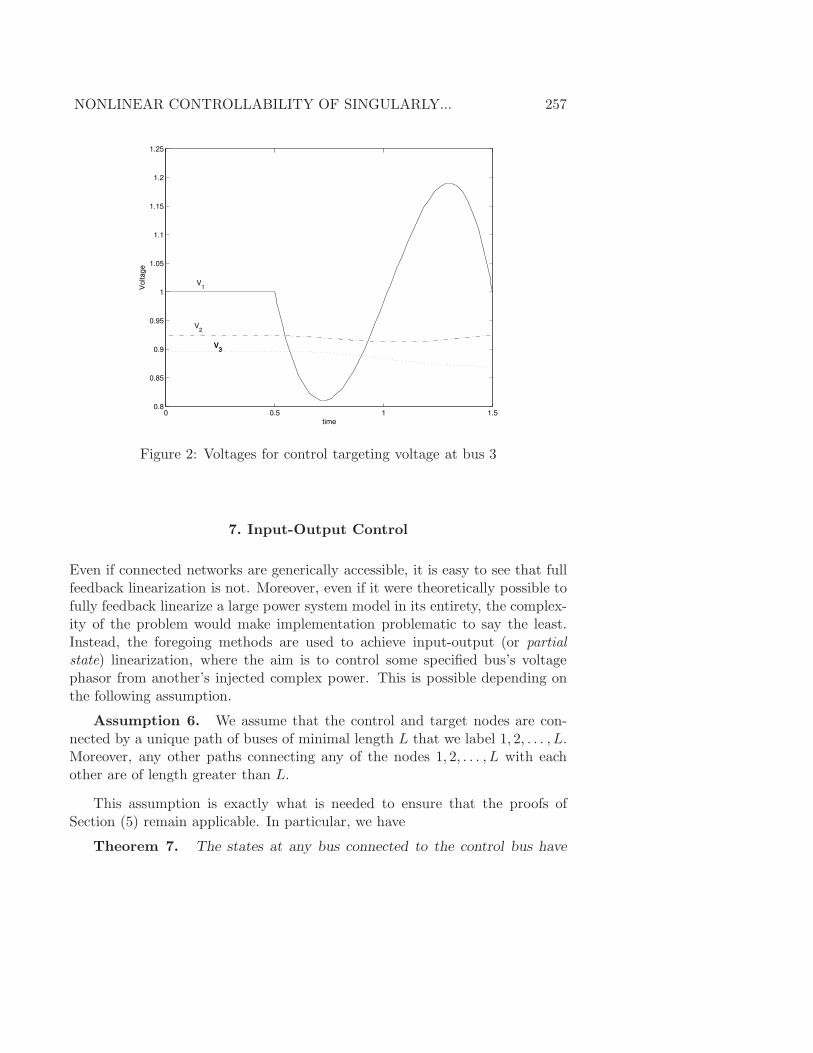
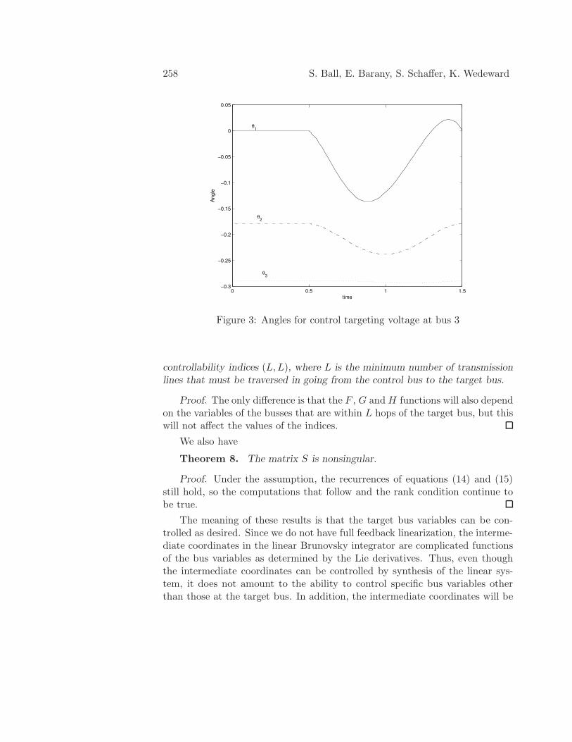
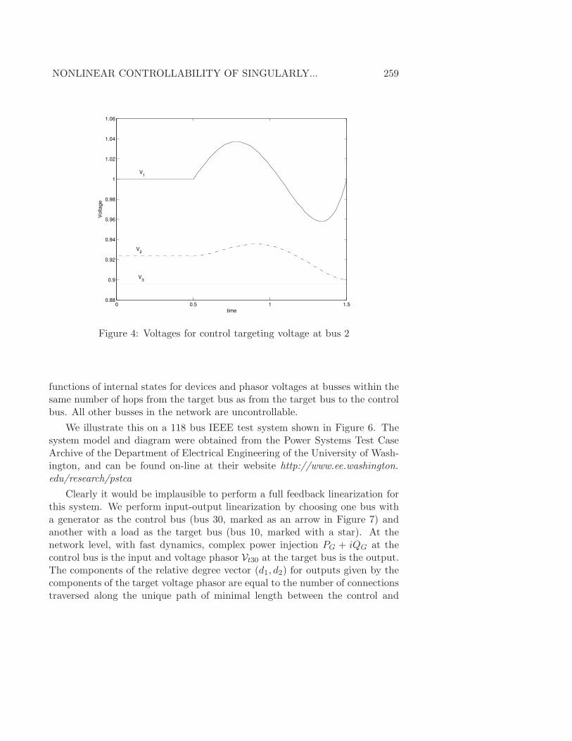
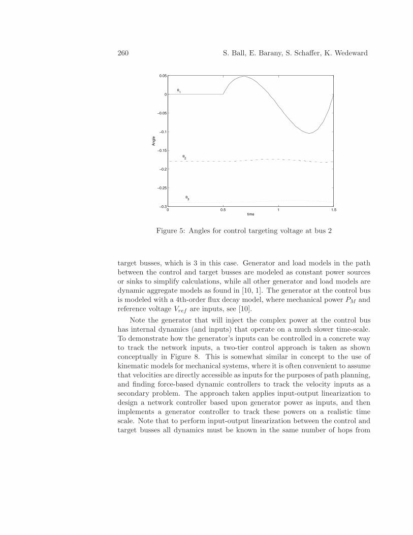
Since the full system is feedback linearizable, the numerical examples aredesigned to show that the system can be moved in any direction in state spacein any specified time. We arbitrarily choose the following two control goals.First we lower the voltage of bus 3 to 0.87 in one second while returning theremaining states to their equilibrium values. This is shown in Figures 2 and3 with the control applied from 0.5 second to 1.5 seconds. Next we lower thevoltage of bus 2 to 0.9, similarly, as shown in Figures 4 and 5.


0 0.5 1 1.50.8

0.85

0.9

0.95

1

1.05

1.1

1.15

1.2

1.25

time

Voltage

V1

V2

0 0.5 1 1.50.8

0.85

0.9

0.95

1

1.05

1.1

1.15

1.2

1.25

time

Voltage

V1

V2

V3

V3

Figure 2: Voltages for control targeting voltage at bus 3

7. Input-Output Control

Even if connected networks are generically accessible, it is easy to see that fullfeedback linearization is not. Moreover, even if it were theoretically possible tofully feedback linearize a large power system model in its entirety, the complex-ity of the problem would make implementation problematic to say the least.Instead, the foregoing methods are used to achieve input-output (or partialstate) linearization, where the aim is to control some specified bus’s voltagephasor from another’s injected complex power. This is possible depending onthe following assumption.

Assumption 6. We assume that the control and target nodes are con-nected by a unique path of buses of minimal length L that we label 1, 2, . . . , L.Moreover, any other paths connecting any of the nodes 1, 2, . . . , L with eachother are of length greater than L.

This assumption is exactly what is needed to ensure that the proofs ofSection (5) remain applicable. In particular, we have

Theorem 7. The states at any bus connected to the control bus have


0 0.5 1 1.5−0.3

−0.25

−0.2

−0.15

−0.1

−0.05

0

0.05

time

Angle

θ1

θ2

θ3

Figure 3: Angles for control targeting voltage at bus 3

controllability indices (L,L), where L is the minimum number of transmissionlines that must be traversed in going from the control bus to the target bus.

Proof. The only difference is that the F , G and H functions will also dependon the variables of the busses that are within L hops of the target bus, but thiswill not affect the values of the indices.

We also have

Theorem 8. The matrix S is nonsingular.

Proof. Under the assumption, the recurrences of equations (14) and (15)still hold, so the computations that follow and the rank condition continue tobe true.

The meaning of these results is that the target bus variables can be con-trolled as desired. Since we do not have full feedback linearization, the interme-diate coordinates in the linear Brunovsky integrator are complicated functionsof the bus variables as determined by the Lie derivatives. Thus, even thoughthe intermediate coordinates can be controlled by synthesis of the linear sys-tem, it does not amount to the ability to control specific bus variables otherthan those at the target bus. In addition, the intermediate coordinates will be


0 0.5 1 1.50.88

0.9

0.92

0.94

0.96

0.98

1

1.02

1.04

1.06

time

Voltage

V1

V2

V3

Figure 4: Voltages for control targeting voltage at bus 2

functions of internal states for devices and phasor voltages at busses within thesame number of hops from the target bus as from the target bus to the controlbus. All other busses in the network are uncontrollable.

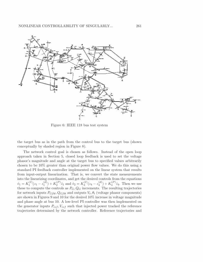
We illustrate this on a 118 bus IEEE test system shown in Figure 6. Thesystem model and diagram were obtained from the Power Systems Test CaseArchive of the Department of Electrical Engineering of the University of Wash-ington, and can be found on-line at their website http://www.ee.washington.edu/research/pstca

Clearly it would be implausible to perform a full feedback linearization forthis system. We perform input-output linearization by choosing one bus witha generator as the control bus (bus 30, marked as an arrow in Figure 7) andanother with a load as the target bus (bus 10, marked with a star). At thenetwork level, with fast dynamics, complex power injection PG + iQG at thecontrol bus is the input and voltage phasor Vt30 at the target bus is the output.The components of the relative degree vector (d1, d2) for outputs given by thecomponents of the target voltage phasor are equal to the number of connectionstraversed along the unique path of minimal length between the control and


0 0.5 1 1.5−0.3

−0.25

−0.2

−0.15

−0.1

−0.05

0

0.05

time

Angle

θ1

θ2

θ3

Figure 5: Angles for control targeting voltage at bus 2

target busses, which is 3 in this case. Generator and load models in the pathbetween the control and target busses are modeled as constant power sourcesor sinks to simplify calculations, while all other generator and load models aredynamic aggregate models as found in [10, 1]. The generator at the control busis modeled with a 4th-order flux decay model, where mechanical power PM andreference voltage Vref are inputs, see [10].

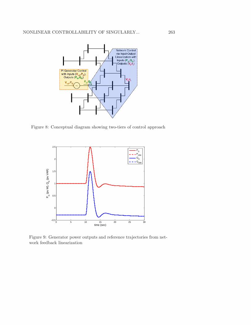
Note the generator that will inject the complex power at the control bushas internal dynamics (and inputs) that operate on a much slower time-scale.To demonstrate how the generator’s inputs can be controlled in a concrete wayto track the network inputs, a two-tier control approach is taken as shownconceptually in Figure 8. This is somewhat similar in concept to the use ofkinematic models for mechanical systems, where it is often convenient to assumethat velocities are directly accessible as inputs for the purposes of path planning,and finding force-based dynamic controllers to track the velocity inputs as asecondary problem. The approach taken applies input-output linearization todesign a network controller based upon generator power as inputs, and thenimplements a generator controller to track these powers on a realistic timescale. Note that to perform input-output linearization between the control andtarget busses all dynamics must be known in the same number of hops from


Figure 6: IEEE 118 bus test system

the target bus as in the path from the control bus to the target bus (shownconceptually by shaded region in Figure 8).

The network control goal is chosen as follows. Instead of the open loopapproach taken in Section 5, closed loop feedback is used to set the voltagephasor’s magnitude and angle at the target bus to specified values arbitrarilychosen to be 10% greater than original power flow values. We do this using astandard PI feedback controller implemented on the linear system that resultsfrom input-output linearization. That is, we convert the state measurementsinto the linearizing coordinates, and get the desired controls from the equations

v1 = K(I)1 (z1 − z

(d)1 ) + K

(P )2 z1 and v2 = K

(I)3 (z4 − z

(d)4 ) + K

(P )4 z4. Then we use

these to compute the controls as PG, QG increments. The resulting trajectoriesfor network inputs PGfbl, QGfbl and outputs Vt, θt (voltage phasor components)are shown in Figures 9 and 10 for the desired 10% increase in voltage magnitudeand phase angle at bus 10. A low-level PI controller was then implemented onthe generator inputs Pref , Vref such that injected power tracked the referencetrajectories determined by the network controller. Reference trajectories and


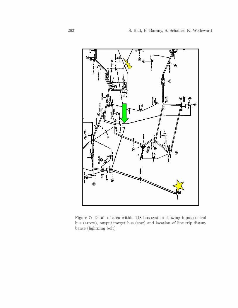
Figure 7: Detail of area within 118 bus system showing input-controlbus (arrow), output/target bus (star) and location of line trip distur-bance (lightning bolt)


Figure 8: Conceptual diagram showing two-tiers of control approach

0 5 10 15 20 25 30−0.5

0

0.5

1

1.5

2

2.5

time (sec)

PG

(pu

W),

QG

(pu

VA

R)

P

G

PGfbl

QG

QGfbl

Figure 9: Generator power outputs and reference trajectories from net-work feedback linearization


0 5 10 15 20 25 30−0.2

0

0.2

0.4

0.6

0.8

1

1.2

time (sec)

Vt1

0 (pu

), θ

t10 (

rad)

V

t10

θt10

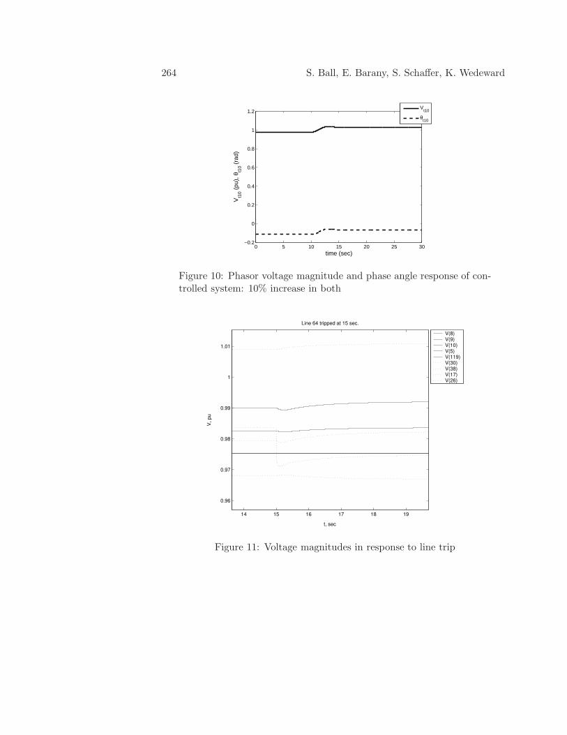
Figure 10: Phasor voltage magnitude and phase angle response of con-trolled system: 10% increase in both

14 15 16 17 18 19

0.96

0.97

0.98

0.99

1

1.01

Line 64 tripped at 15 sec.

t, sec

V, p

u

V(8)V(9)V(10)V(5)V(119)V(30)V(38)V(17)V(26)

Figure 11: Voltage magnitudes in response to line trip


generator outputs are shown in Figure 9 with resulting response at the targetbus shown in Figure 10.

Finally, results indicative of the robustness of the control strategy are pre-sented. A disturbance was introduced in the system by tripping a transmissionline (indicated by a lightning bolt on Figure 7) outside the region, where pre-cise knowledge is needed for the input-output linearization. Figure 11 showsthe system restabilizing after the trip event in such a way that the voltage mag-nitude at the target bus (bus 10) remains exactly at its desired value. Similarbehavior was seen in simulations for which other lines were tripped.

8. Conclusions

In this paper an approach was presented for analyzing the effects that bussesof a power system have on each other due to the network structure. The initialgoal has been to model the system as simply as possible based on the powerflow equations and show that the apparatus of differential geometric controlcan be applied to the problem of controlling the states of one bus by adjustingthe power inputs of another. A simple chain network was considered, wherethese tools worked out particularly well due to the fact that the system is fullyfeedback linearizable. Then from a more general perspective, similar methodswere applied in the context of input-output decoupling for a 118 bus IEEE testsystem.

References

[1] P. Anderson, A. Fouad, Power System Control and Stability, Iowa StateUniversity Press (1977).

[2] R.J. Davy, I.A. Hiskens, Lyapunov functions for multimachine power sys-tems with dynamic loads, IEEE Trans. on Circuits and Systems-I, 44, No.9 (1997), 796-812.

[3] M. Hong, C. Liu, M. Gibescu, Complete controllability of an N-bus dy-namic power system model, IEEE Trans. on Circuits and Systems-I, 46,No. 6 (1999), 700-713.

[4] M.D. Ilic, E.H. Allen, J.W. Chapman, C.A. King, J.H. Lang, E. Litvinov,Preventing future blackouts by means of enhanced electric power systems


control: From complexity to order, Proceedings of the IEEE, 93, No. 11(2005), (1920)-(1940).

[5] M. Ilic, J. Zaborsky, Dynamics and Control of Large Electric Power Sys-tems, Wiley-Interscience, New York (2000).

[6] A. Isidori, Nonlinear Control Systems, Second Edition, Springer-Verlag,New York (1989).

[7] H. Nijmeijer, A. van der Schaft, Nonlinear Dynamical Control Systems,Springer-Verlag, New York (1990).

[8] K.L. Praprost, K.A. Loparo, Energy function method for determining volt-age collapse during a power system transient, IEEE Trans. on Circuits andSystems-I, 41, No. 10 (1994), 635-651.

[9] S.S. Sastry, C.A. Desoer, Jump behavior of circuits and systems, IEEETrans. on Circuits and Systems, CAS-28, No. 12 (1981), 1109-1124.

[10] P. Sauer, M. Pai, Power System Dynamics and Stability, Prentice Hall,Englewood Cliffs, New Jersey (1998).

[11] F. Takens, Singularities of vector fields, Inst. Hautes Etudes Sci. Publ.Math., 43 (1974), 47-100.

[12] V. Venkatasubramanian, H. Schattler, J. Zaborszky, Fast time-varyingphasor analysis in the balanced three-phase large electric power system,IEEE Trans. on Automatic Control, 40, No. 11 (1995), (1975)-(1982).

[13] M. Vidyasagar, Nonlinear Systems Analysis, Second Edition, Prentice Hall,Englewood Cliffs, New Jersey (1993).

[14] D.J. Watts, S.H. Strogatz, Collective dynamics of ‘small-world’ networks,Nature, 393, No. 6684 (1998), 440-442.

Documents

NONLINEAR CONTROLLABILITY OF SINGULARLY PERTURBED