Embed Size (px)
Citation preview
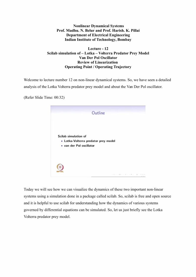
Nonlinear Dynamical SystemsProf. Madhu. N. Belur and Prof. Harish. K. Pillai
Department of Electrical EngineeringIndian Institute of Technology, Bombay
Lecture - 12Scilab simulation of – Lotka – Volterra Predator Prey Model
Van Der Pol Oscillator Review of Linearization
Operating Point / Operating Trajectory
Welcome to lecture number 12 on non-linear dynamical systems. So, we have seen a detailed
analysis of the Lotka Volterra predator prey model and about the Van Der Pol oscillator.
(Refer Slide Time: 00:32)
Today we will see how we can visualize the dynamics of these two important non-linear
systems using a simulation done in a package called scilab. So, scilab is free and open source
and it is helpful to use scilab for understanding how the dynamics of various systems
governed by differential equations can be simulated. So, let us just briefly see the Lotka
Volterra predator prey model.
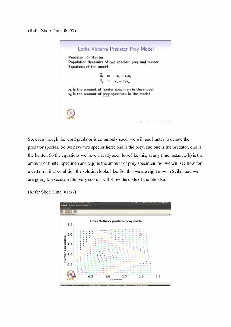
(Refer Slide Time: 00:57)
So, even though the word predator is commonly used, we will use hunter to denote the
predator species. So we have two species here: one is the prey, and one is the predator, one is
the hunter. So the equations we have already seen look like this; at any time instant x(h) is the
amount of hunter specimen and x(p) is the amount of prey specimen. So, we will see how for
a certain initial condition the solution looks like. So, this we are right now in Scilab and we
are going to execute a file; very soon, I will show the code of the file also.
(Refer Slide Time: 01:37)
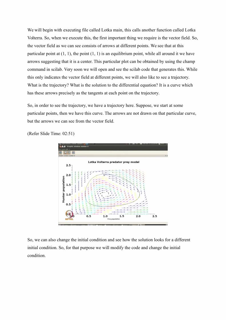
We will begin with executing file called Lotka main, this calls another function called Lotka
Volterra. So, when we execute this, the first important thing we require is the vector field. So,
the vector field as we can see consists of arrows at different points. We see that at this
particular point at (1, 1), the point (1, 1) is an equilibrium point, while all around it we have
arrows suggesting that it is a center. This particular plot can be obtained by using the champ
command in scilab. Very soon we will open and see the scilab code that generates this. While
this only indicates the vector field at different points, we will also like to see a trajectory.
What is the trajectory? What is the solution to the differential equation? It is a curve which
has these arrows precisely as the tangents at each point on the trajectory.
So, in order to see the trajectory, we have a trajectory here. Suppose, we start at some
particular points, then we have this curve. The arrows are not drawn on that particular curve,
but the arrows we can see from the vector field.
(Refer Slide Time: 02:51)
So, we can also change the initial condition and see how the solution looks for a different
initial condition. So, for that purpose we will modify the code and change the initial
condition.
(Refer Slide Time: 03:17)
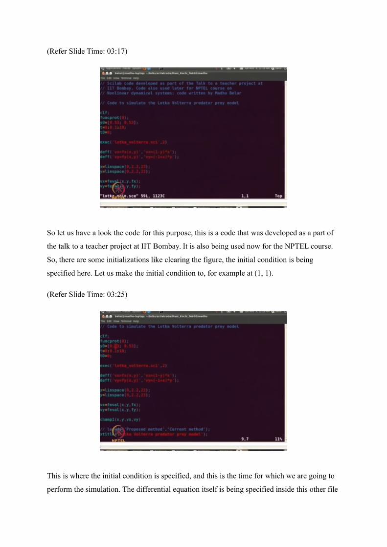
So let us have a look the code for this purpose, this is a code that was developed as a part of
the talk to a teacher project at IIT Bombay. It is also being used now for the NPTEL course.
So, there are some initializations like clearing the figure, the initial condition is being
specified here. Let us make the initial condition to, for example at (1, 1).
(Refer Slide Time: 03:25)
This is where the initial condition is specified, and this is the time for which we are going to
perform the simulation. The differential equation itself is being specified inside this other file
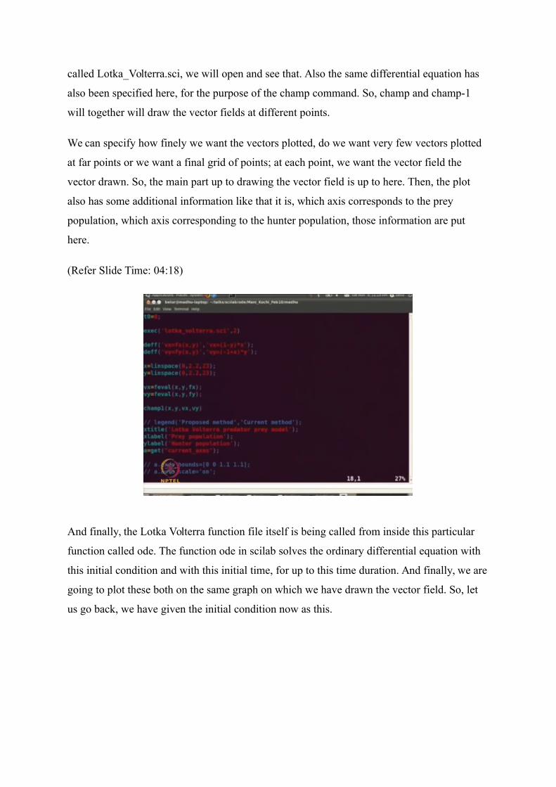
called Lotka_Volterra.sci, we will open and see that. Also the same differential equation has
also been specified here, for the purpose of the champ command. So, champ and champ-1
will together will draw the vector fields at different points.
We can specify how finely we want the vectors plotted, do we want very few vectors plotted
at far points or we want a final grid of points; at each point, we want the vector field the
vector drawn. So, the main part up to drawing the vector field is up to here. Then, the plot
also has some additional information like that it is, which axis corresponds to the prey
population, which axis corresponding to the hunter population, those information are put
here.
(Refer Slide Time: 04:18)
And finally, the Lotka Volterra function file itself is being called from inside this particular
function called ode. The function ode in scilab solves the ordinary differential equation with
this initial condition and with this initial time, for up to this time duration. And finally, we are
going to plot these both on the same graph on which we have drawn the vector field. So, let
us go back, we have given the initial condition now as this.
(Refer Slide Time: 05:23)
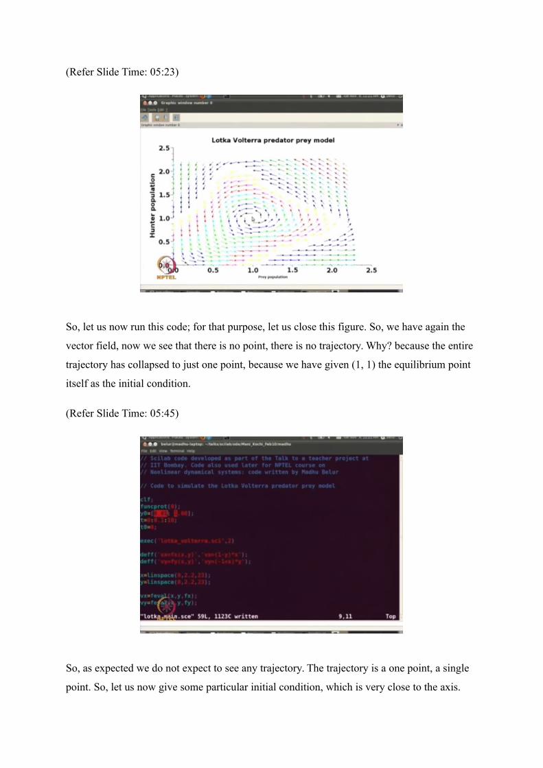
So, let us now run this code; for that purpose, let us close this figure. So, we have again the
vector field, now we see that there is no point, there is no trajectory. Why? because the entire
trajectory has collapsed to just one point, because we have given (1, 1) the equilibrium point
itself as the initial condition.
(Refer Slide Time: 05:45)
So, as expected we do not expect to see any trajectory. The trajectory is a one point, a single
point. So, let us now give some particular initial condition, which is very close to the axis.
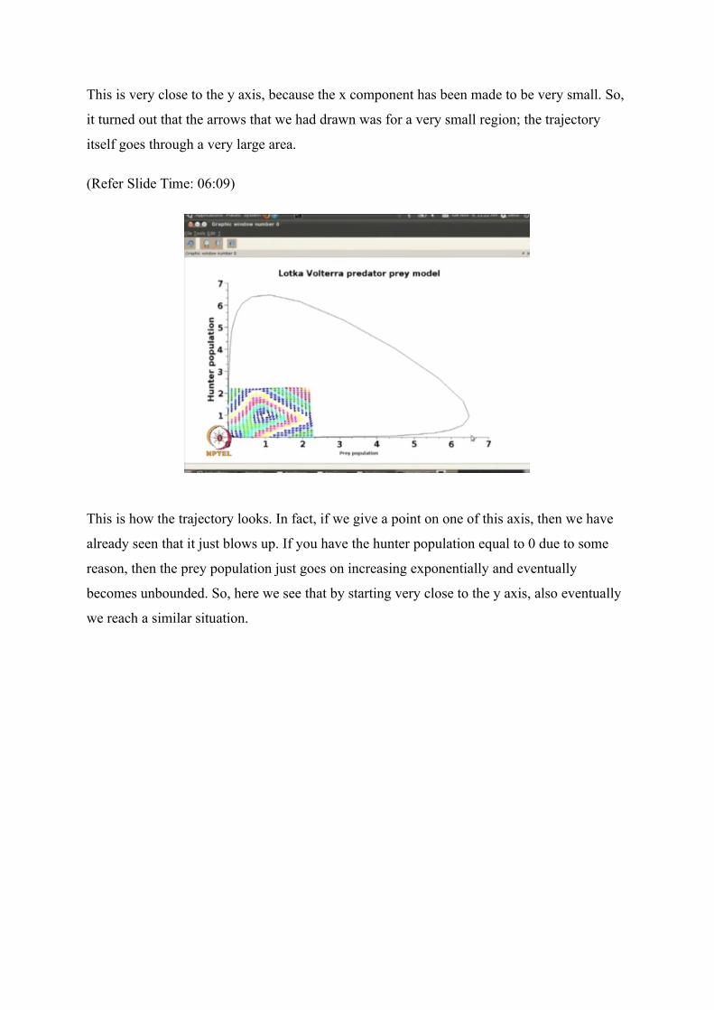
This is very close to the y axis, because the x component has been made to be very small. So,
it turned out that the arrows that we had drawn was for a very small region; the trajectory
itself goes through a very large area.
(Refer Slide Time: 06:09)
This is how the trajectory looks. In fact, if we give a point on one of this axis, then we have
already seen that it just blows up. If you have the hunter population equal to 0 due to some
reason, then the prey population just goes on increasing exponentially and eventually
becomes unbounded. So, here we see that by starting very close to the y axis, also eventually
we reach a similar situation.
(Refer Slide Time: 06:52)
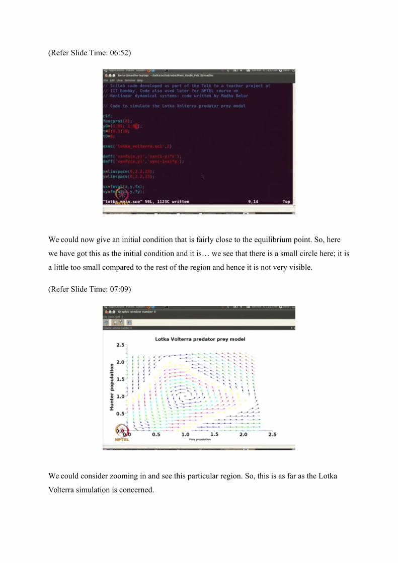
We could now give an initial condition that is fairly close to the equilibrium point. So, here
we have got this as the initial condition and it is… we see that there is a small circle here; it is
a little too small compared to the rest of the region and hence it is not very visible.
(Refer Slide Time: 07:09)
We could consider zooming in and see this particular region. So, this is as far as the Lotka
Volterra simulation is concerned.
(Refer Slide Time: 07:36)
We were to also see this particular, this other file. So, this is just the function; it defines given
x, what is x dot, x dot is nothing but f(x). So, f is getting defined inside this function.
(Refer Slide Time: 07:48)
(Refer Slide Time: 07:51)
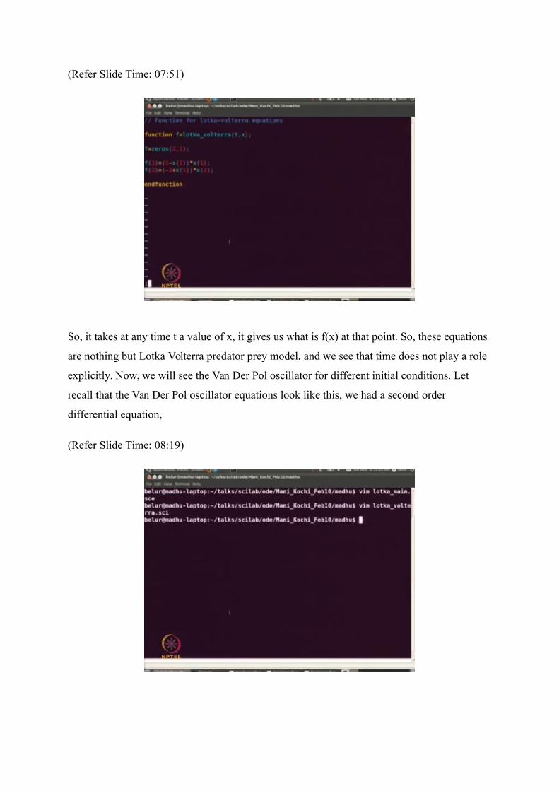
So, it takes at any time t a value of x, it gives us what is f(x) at that point. So, these equations
are nothing but Lotka Volterra predator prey model, and we see that time does not play a role
explicitly. Now, we will see the Van Der Pol oscillator for different initial conditions. Let
recall that the Van Der Pol oscillator equations look like this, we had a second order
differential equation,
(Refer Slide Time: 08:19)
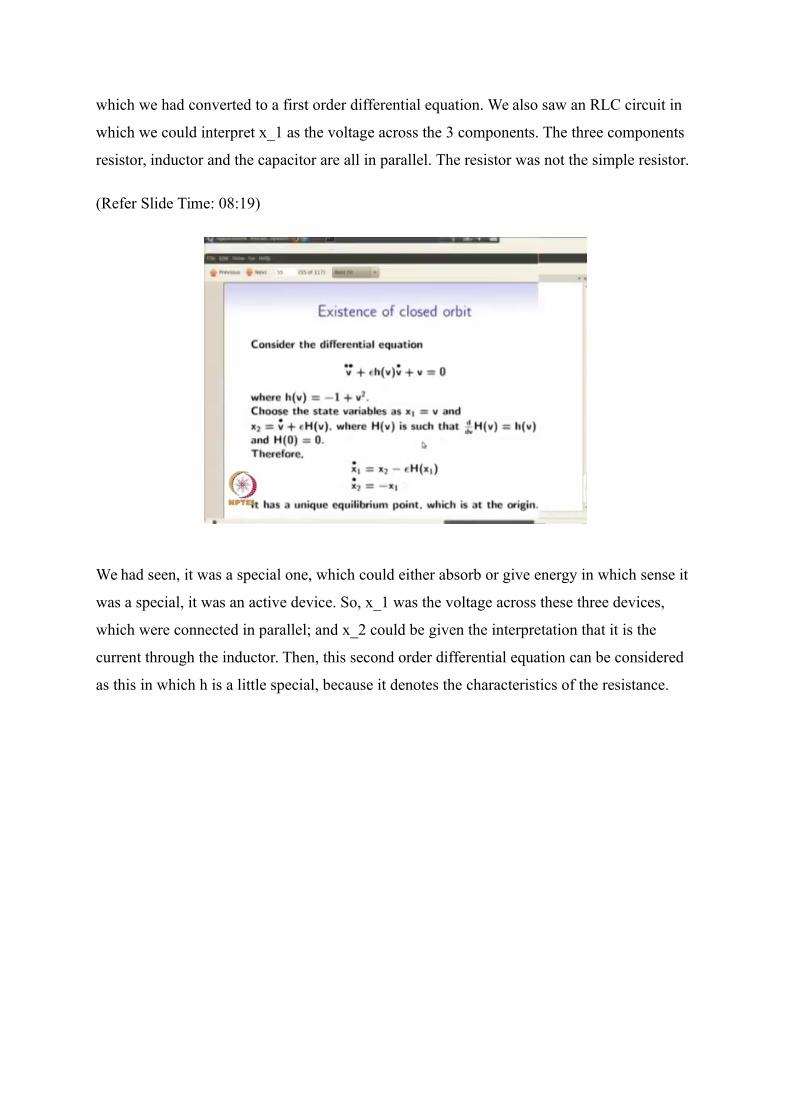
which we had converted to a first order differential equation. We also saw an RLC circuit in
which we could interpret x_1 as the voltage across the 3 components. The three components
resistor, inductor and the capacitor are all in parallel. The resistor was not the simple resistor.
(Refer Slide Time: 08:19)
We had seen, it was a special one, which could either absorb or give energy in which sense it
was a special, it was an active device. So, x_1 was the voltage across these three devices,
which were connected in parallel; and x_2 could be given the interpretation that it is the
current through the inductor. Then, this second order differential equation can be considered
as this in which h is a little special, because it denotes the characteristics of the resistance.
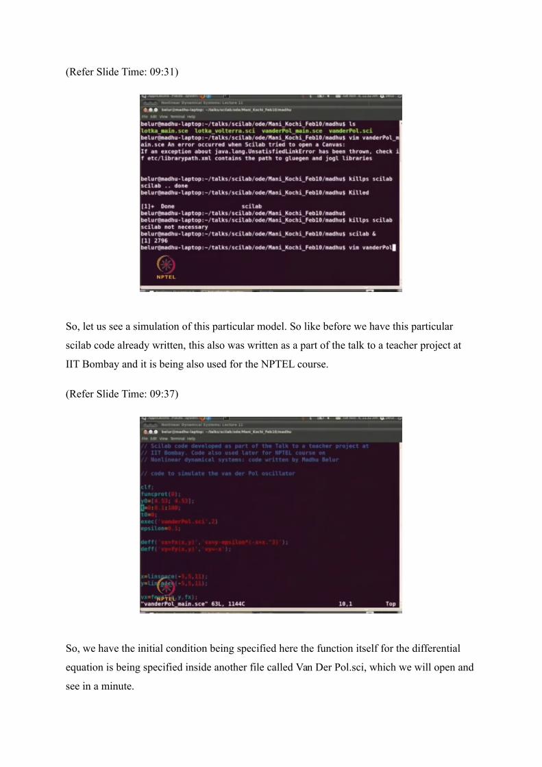
(Refer Slide Time: 09:31)
So, let us see a simulation of this particular model. So like before we have this particular
scilab code already written, this also was written as a part of the talk to a teacher project at
IIT Bombay and it is being also used for the NPTEL course.
(Refer Slide Time: 09:37)
So, we have the initial condition being specified here the function itself for the differential
equation is being specified inside another file called Van Der Pol.sci, which we will open and
see in a minute.
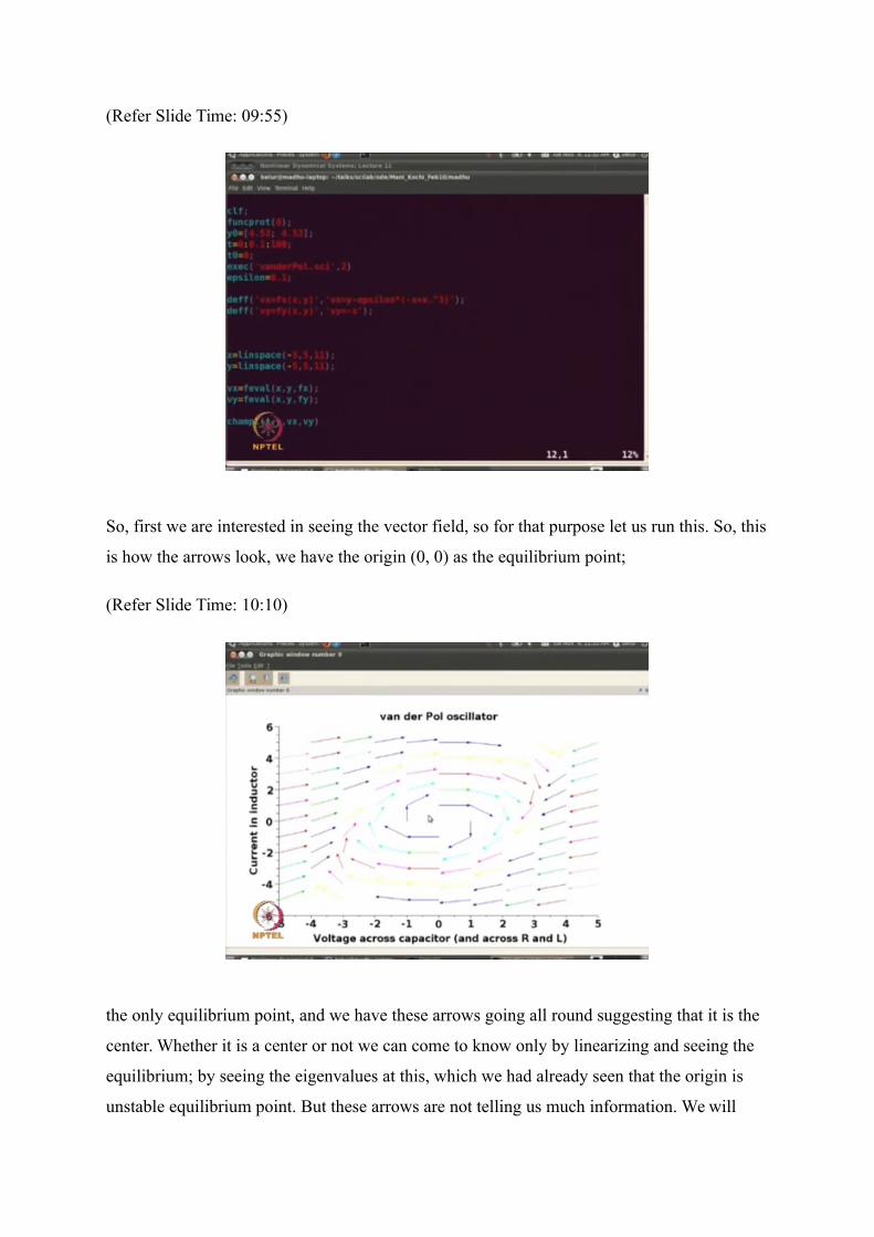
(Refer Slide Time: 09:55)
So, first we are interested in seeing the vector field, so for that purpose let us run this. So, this
is how the arrows look, we have the origin (0, 0) as the equilibrium point;
(Refer Slide Time: 10:10)
the only equilibrium point, and we have these arrows going all round suggesting that it is the
center. Whether it is a center or not we can come to know only by linearizing and seeing the
equilibrium; by seeing the eigenvalues at this, which we had already seen that the origin is
unstable equilibrium point. But these arrows are not telling us much information. We will
also see depending on whether we start from outside or certain limit cycle or inside these
arrows are going to tell whether we will be converging to the limit cycle either from the
inside or the outside.
So, let us… we have already specified an initial condition, first we have seen only the arrows
and it is waiting for our button to be pressed. So, for this particular initial condition the
trajectories are coming closer and closer and encircling round and round, and eventually
converging to this limit cycle. So, that is for the case that we start from this particular point;
we can take another two points also from outside this particular limit cycle.
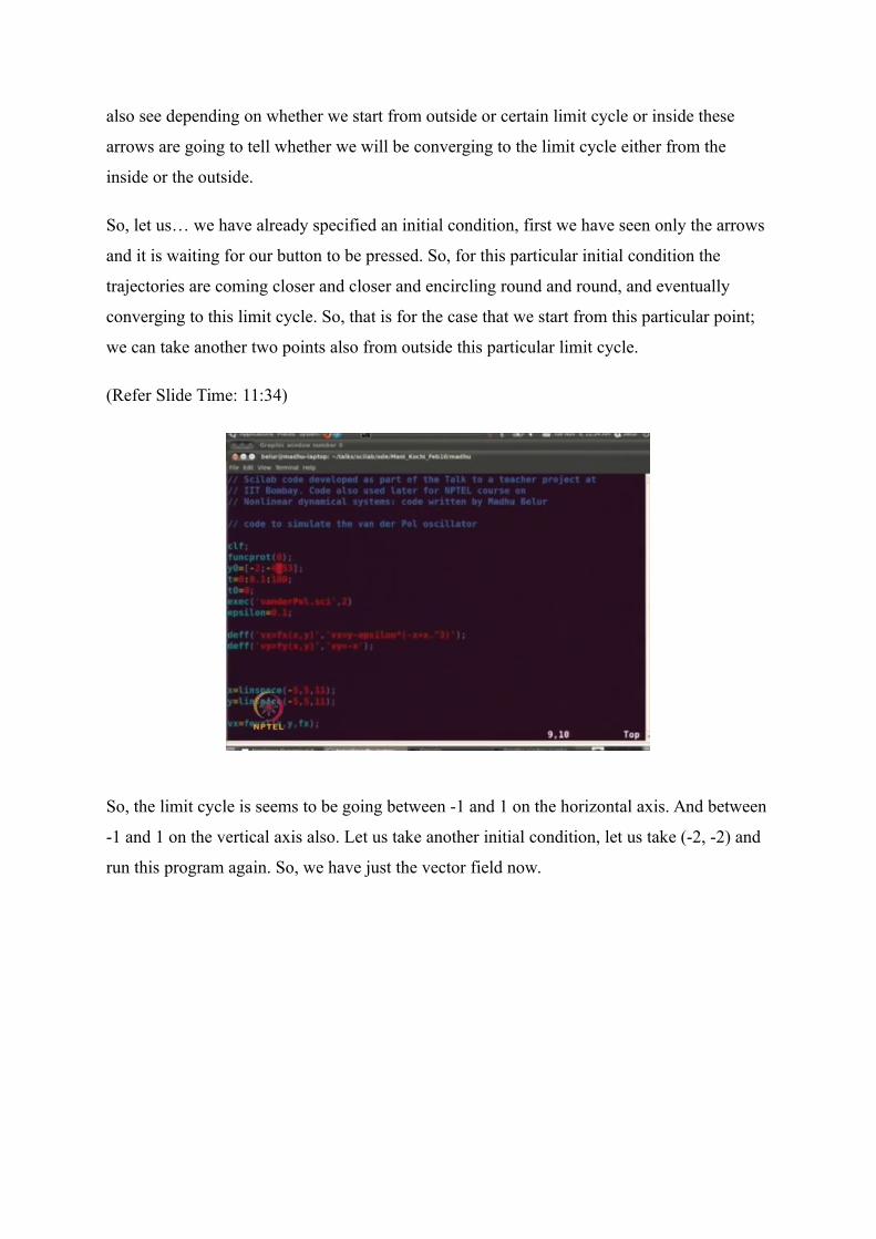
(Refer Slide Time: 11:34)
So, the limit cycle is seems to be going between -1 and 1 on the horizontal axis. And between
-1 and 1 on the vertical axis also. Let us take another initial condition, let us take (-2, -2) and
run this program again. So, we have just the vector field now.
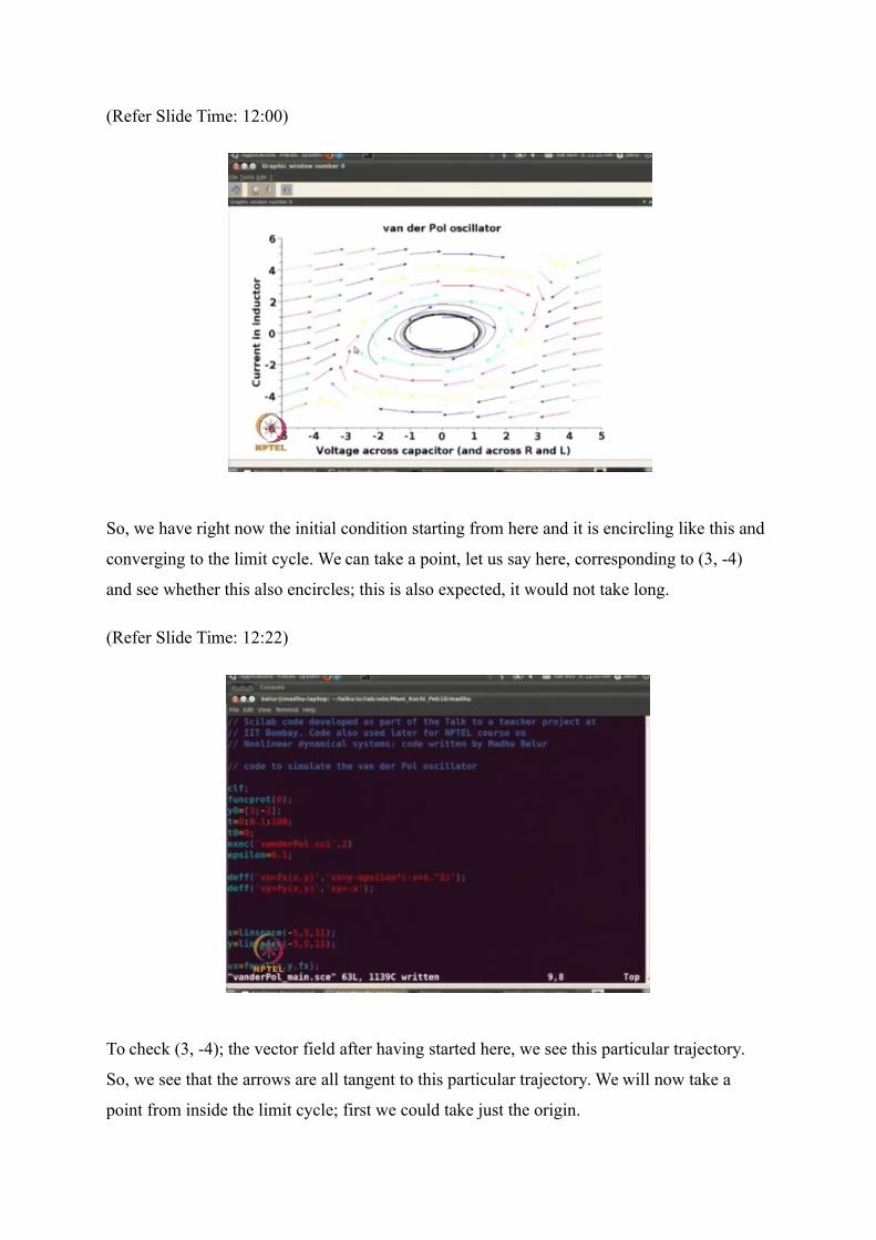
(Refer Slide Time: 12:00)
So, we have right now the initial condition starting from here and it is encircling like this and
converging to the limit cycle. We can take a point, let us say here, corresponding to (3, -4)
and see whether this also encircles; this is also expected, it would not take long.
(Refer Slide Time: 12:22)
To check (3, -4); the vector field after having started here, we see this particular trajectory.
So, we see that the arrows are all tangent to this particular trajectory. We will now take a
point from inside the limit cycle; first we could take just the origin.
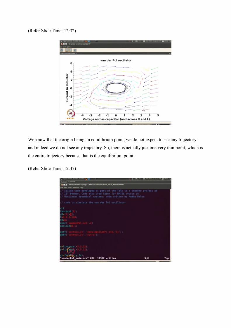
(Refer Slide Time: 12:32)
We know that the origin being an equilibrium point, we do not expect to see any trajectory
and indeed we do not see any trajectory. So, there is actually just one very thin point, which is
the entire trajectory because that is the equilibrium point.
(Refer Slide Time: 12:47)
(Refer Slide Time: 12:55)
(Refer Slide Time: 13:12)
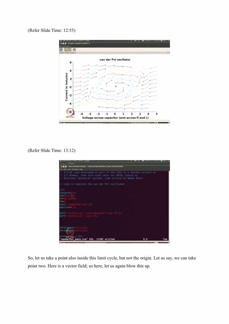
So, let us take a point also inside this limit cycle, but not the origin. Let us say, we can take
point two. Here is a vector field; so here, let us again blow this up.
(Refer Slide Time: 13:20)
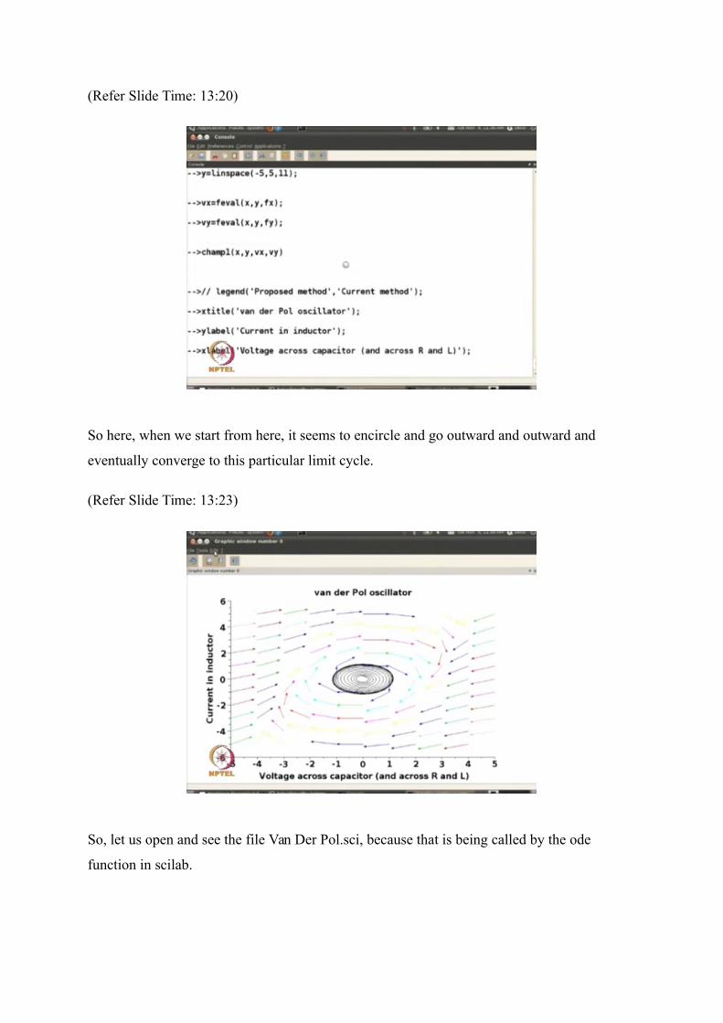
So here, when we start from here, it seems to encircle and go outward and outward and
eventually converge to this particular limit cycle.
(Refer Slide Time: 13:23)
So, let us open and see the file Van Der Pol.sci, because that is being called by the ode
function in scilab.
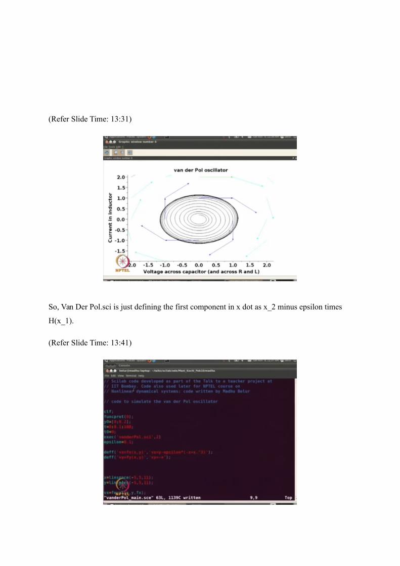
(Refer Slide Time: 13:31)
So, Van Der Pol.sci is just defining the first component in x dot as x_2 minus epsilon times
H(x_1).
(Refer Slide Time: 13:41)
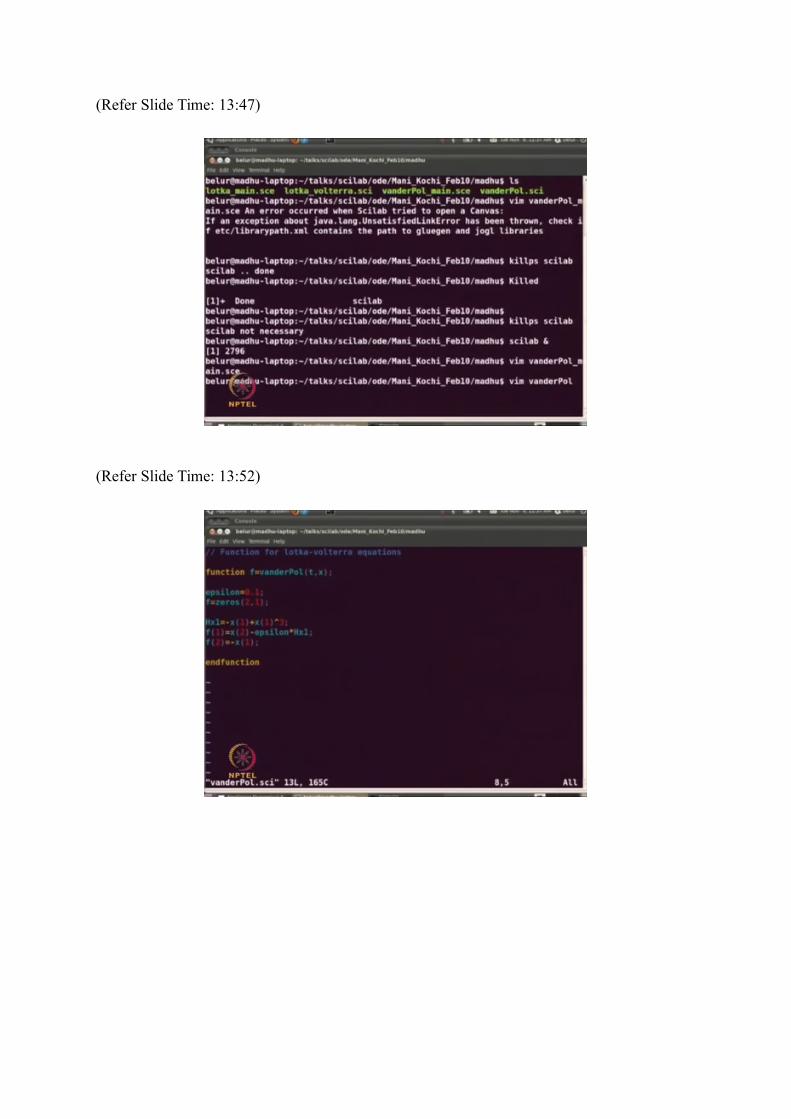
(Refer Slide Time: 13:47)
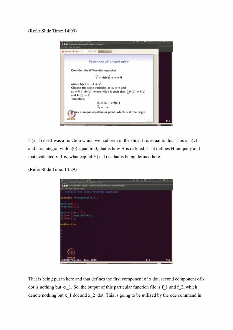
(Refer Slide Time: 13:52)
(Refer Slide Time: 14:09)
H(x_1) itself was a function which we had seen in the slide. It is equal to this. This is h(v)
and it is integral with h(0) equal to 0; that is how H is defined. That defines H uniquely and
that evaluated x_1 is, what capital H(x_1) is that is being defined here.
(Refer Slide Time: 14:29)
That is being put in here and that defines the first component of x dot, second component of x
dot is nothing but -x_1. So, the output of this particular function file is f_1 and f_2, which
denote nothing but x_1 dot and x_2 dot. This is going to be utilized by the ode command in
scilab. So, this explains how we can use scilab to visualize the dynamics of a differential
equation. While a second order differential equation can be visualized using the vector field,
also by using the champ and champ 1 command. More generally, we can use ode command to
see.. to obtain the solution to a differential equation and initial value problem in particular.
(Refer Slide Time: 15:13)
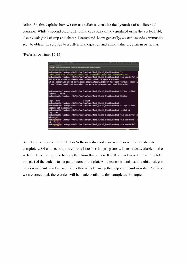
So, let us like we did for the Lotka Volterra scilab code, we will also see the scilab code
completely. Of course, both the codes all the 4 scilab programs will be made available on the
website. It is not required to copy this from this screen. It will be made available completely,
this part of the code is to set parameters of the plot. All these commands can be obtained, can
be seen in detail, can be used more effectively by using the help command in scilab. As far as
we are concerned, these codes will be made available, this completes this topic.
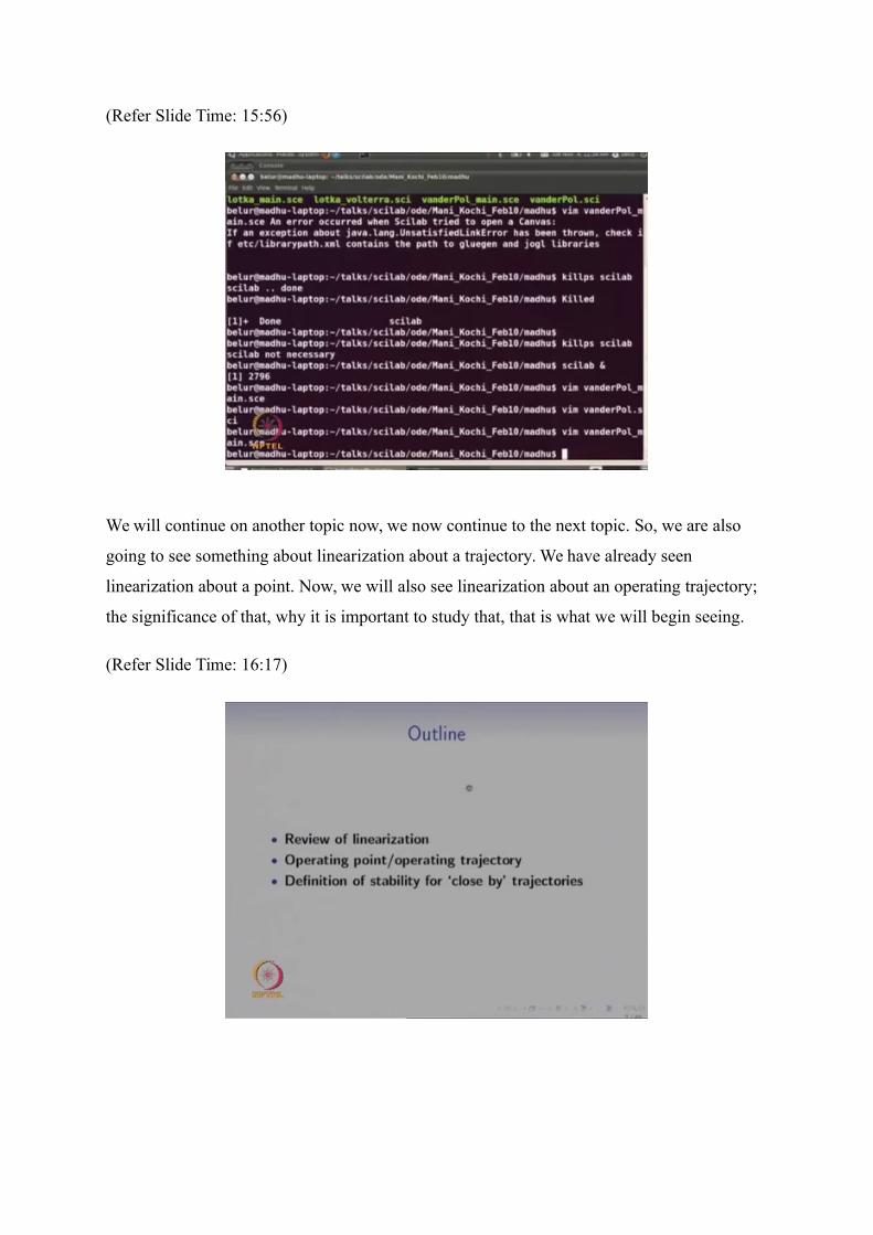
(Refer Slide Time: 15:56)
We will continue on another topic now, we now continue to the next topic. So, we are also
going to see something about linearization about a trajectory. We have already seen
linearization about a point. Now, we will also see linearization about an operating trajectory;
the significance of that, why it is important to study that, that is what we will begin seeing.
(Refer Slide Time: 16:17)
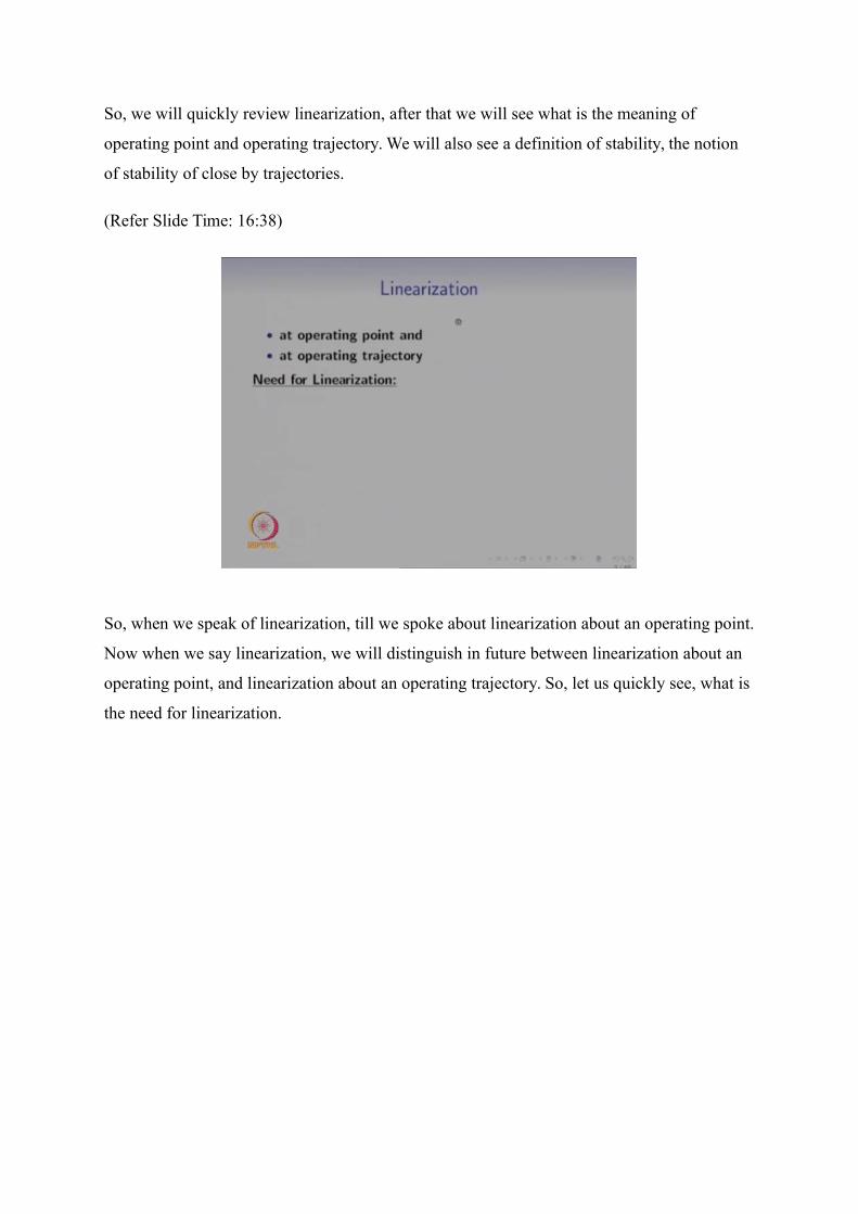
So, we will quickly review linearization, after that we will see what is the meaning of
operating point and operating trajectory. We will also see a definition of stability, the notion
of stability of close by trajectories.
(Refer Slide Time: 16:38)
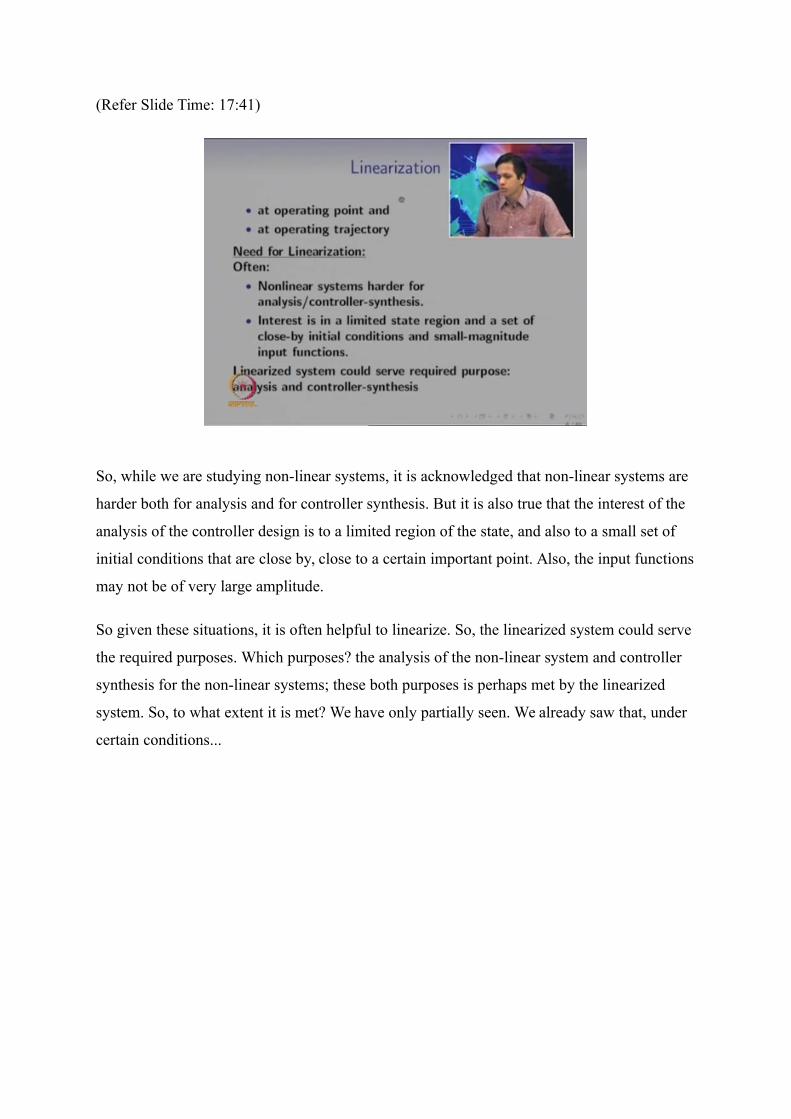
So, when we speak of linearization, till we spoke about linearization about an operating point.
Now when we say linearization, we will distinguish in future between linearization about an
operating point, and linearization about an operating trajectory. So, let us quickly see, what is
the need for linearization.
(Refer Slide Time: 17:41)
So, while we are studying non-linear systems, it is acknowledged that non-linear systems are
harder both for analysis and for controller synthesis. But it is also true that the interest of the
analysis of the controller design is to a limited region of the state, and also to a small set of
initial conditions that are close by, close to a certain important point. Also, the input functions
may not be of very large amplitude.
So given these situations, it is often helpful to linearize. So, the linearized system could serve
the required purposes. Which purposes? the analysis of the non-linear system and controller
synthesis for the non-linear systems; these both purposes is perhaps met by the linearized
system. So, to what extent it is met? We have only partially seen. We already saw that, under
certain conditions...
(Refer Slide Time: 18:03)
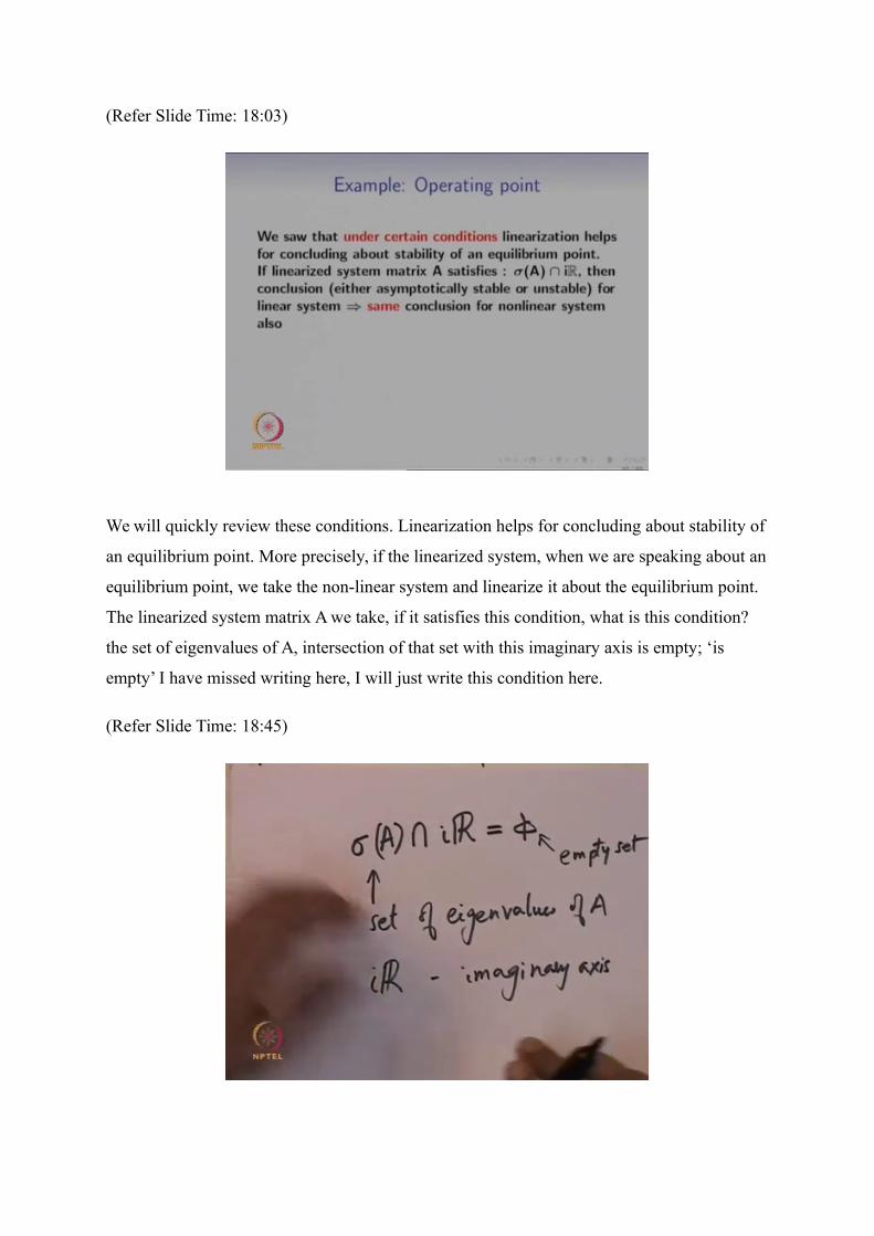
We will quickly review these conditions. Linearization helps for concluding about stability of
an equilibrium point. More precisely, if the linearized system, when we are speaking about an
equilibrium point, we take the non-linear system and linearize it about the equilibrium point.
The linearized system matrix A we take, if it satisfies this condition, what is this condition?
the set of eigenvalues of A, intersection of that set with this imaginary axis is empty; ‘is
empty’ I have missed writing here, I will just write this condition here.
(Refer Slide Time: 18:45)
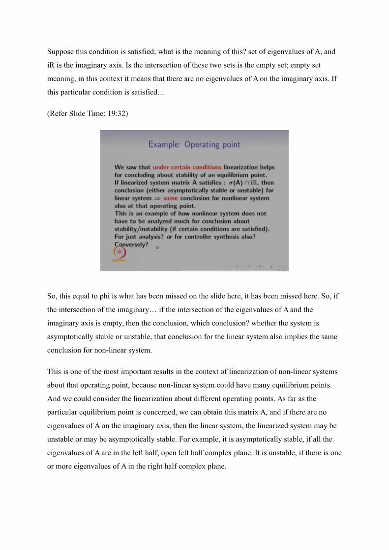
Suppose this condition is satisfied; what is the meaning of this? set of eigenvalues of A, and
iR is the imaginary axis. Is the intersection of these two sets is the empty set; empty set
meaning, in this context it means that there are no eigenvalues of A on the imaginary axis. If
this particular condition is satisfied…
(Refer Slide Time: 19:32)
So, this equal to phi is what has been missed on the slide here, it has been missed here. So, if
the intersection of the imaginary… if the intersection of the eigenvalues of A and the
imaginary axis is empty, then the conclusion, which conclusion? whether the system is
asymptotically stable or unstable, that conclusion for the linear system also implies the same
conclusion for non-linear system.
This is one of the most important results in the context of linearization of non-linear systems
about that operating point, because non-linear system could have many equilibrium points.
And we could consider the linearization about different operating points. As far as the
particular equilibrium point is concerned, we can obtain this matrix A, and if there are no
eigenvalues of A on the imaginary axis, then the linear system, the linearized system may be
unstable or may be asymptotically stable. For example, it is asymptotically stable, if all the
eigenvalues of A are in the left half, open left half complex plane. It is unstable, if there is one
or more eigenvalues of A in the right half complex plane.
So, this particular conclusion on the linearized system, we are able to do using the linearized
system matrix A; that conclusion is the same for the non-linear system also about the
equilibrium point under this condition. Under which condition? under the condition that there
are no eigenvalues of A on the imaginary axis. So, what is the significance of this? This is an
example of how non-linear system does not have to be analyzed much. As far as this
particular conclusion goes, as far as the conclusion whether the non-linear system about an
equilibrium point is unstable or asymptotically stable, as far as that conclusion goes, it is
enough to study the linearized system.
This conclusion is indeed the same only under certain conditions, only when certain
conditions are satisfied. If those conditions are not satisfied, then it is not possible to say that
the same conclusion holds. Now, we can ask, is this something that is just for analysis or is
this going to help for controller synthesis also? Is it that such a result can also be utilized for
controller synthesis? This is something that we will see in the detail in the next few lectures.
Another important thing is, what about converse; if you know that the non-linear system is
unstable, is it true that the linearized system is also unstable; that is the other question when
what we refer to here as conversely. So, these are important questions that we will address in
the next few lectures; we will address the notion of controller synthesis for the linearized
system, and whether that controller will work for the non-linear system also.
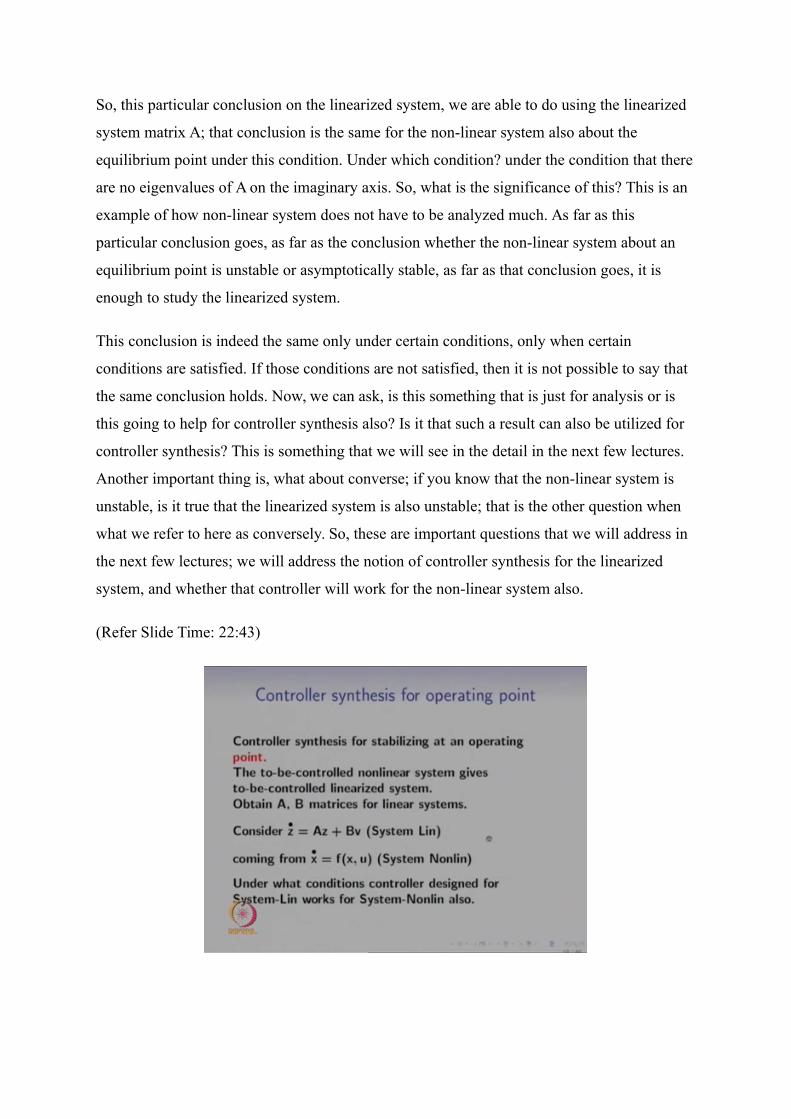
(Refer Slide Time: 22:43)
So, let us come back to this question, controller synthesis for stabilizing a non-linear system
at an operating point. As I said, when we say operating point, we need to know, distinguish
that operating trajectory and operating point in the context of linearization. So, let us first ask
this question, controller synthesis for stabilizing a non-linear system about an operating point.
So, that to be controlled non-linear system gives a to be controlled linearized system. Upon
linearization of the non-linear system which had some inputs will give us a linearized system
also with some inputs.
So, suppose A and B are matrices for the linear system… We will do this in a little more
precise way; in the next few lectures, I am just motivating how a controller for the linearized
system may work for the non-linear system also. Suppose, A and B are matrices for the
linearized system. Let us call system Lin and these matrices A and B are coming from the
non-linear system x dot is equal to f(x, u). Till now we had been studying only autonomous
systems; there was no input u nor v. Now, we are speaking of a system which allows you to
put a control input.
So, the linearized system is this, in which the state has been called z; z dot is equal to z plus
Bv and the original non-linear system was x dot is equal to f(x, u). We will see how A and B
matrices are to be obtained from this particular function f. Under what conditions, so what is
the controller synthesis question, under what conditions controller designed for system Lin
also works for system Non-lin?
The controller we have designed for this system, under what condition it will work for this
system also. Given that A and B where obtained from these, from this non-linear system, may
be it is possible that linear control theory for this system might automatically hold for this
system also.

(Refer Slide Time: 24:49)
In order to answer this question, we have to understand little more detail about linearization
about an operating trajectory. In the context of linearization, we will also speak about stability
of the operating trajectory. So, we have already seen for an autonomous system, what it
means for stability of an equilibrium point. We also saw Lyapunov stability of the equilibrium
point. Now, the next question is, what is the meaning of stability of an operating trajectory, of
a trajectory? So, let us first consider the case when that trajectory is a periodic orbit.
(Refer Slide Time: 25:30)
So, suppose this is a periodic orbit and now we know that if we start on this periodic orbit,
then we will keep going along this orbit. We could ask the question, is this periodic orbit
stable in the sense that trajectories that start close to this periodic orbit do they converge to
this periodic orbit? This is the question we ask in the context of Van Der Pol oscillator, for
example. We ask whether this periodic orbit is a stable limit cycle; what does it mean to be a
limit cycle?
We have these other trajectories that are converging to this and stable limit cycle means that
we take such a cut and we look at all initial conditions close to this periodic orbit. We could
ask are all these trajectories, which trajectories? all the trajectories that are starting close to
this periodic orbit, are all of them going to converge to this periodic orbit? That is ideally the
case, that is how we want for robust sustained oscillations of an oscillator that we build in a
laboratory.
We want that no matter what initial conditions, it should converge to that periodic orbit,
because that periodic orbit perhaps is carefully designed to have the right period and right
amplitude. So, this is what we will say a limit cycle, a stable limit cycle. A stable limit cycle
is one in which we have a periodic orbit, the cycle itself and trajectories that are close by
come closer and closer to this periodic orbit. Of course, we know that it cannot come and
intersect at any particular point. Why is it that the two trajectories cannot intersect? It can
intersect, this is possible only if the function is not Lipschitz at this point.
If the function is Lipschitz, then we know that the two trajectories cannot intersect. So, we
have all trajectories that are coming close and closer to the stable limit cycle; also from the
inside when they start… So, we have already seen results in this context. So, we already
know what it means for a trajectory to be stable. We informally know it for the purpose of
this limit cycle; for the case of periodic orbit, we already speak about stability of periodic
orbits.
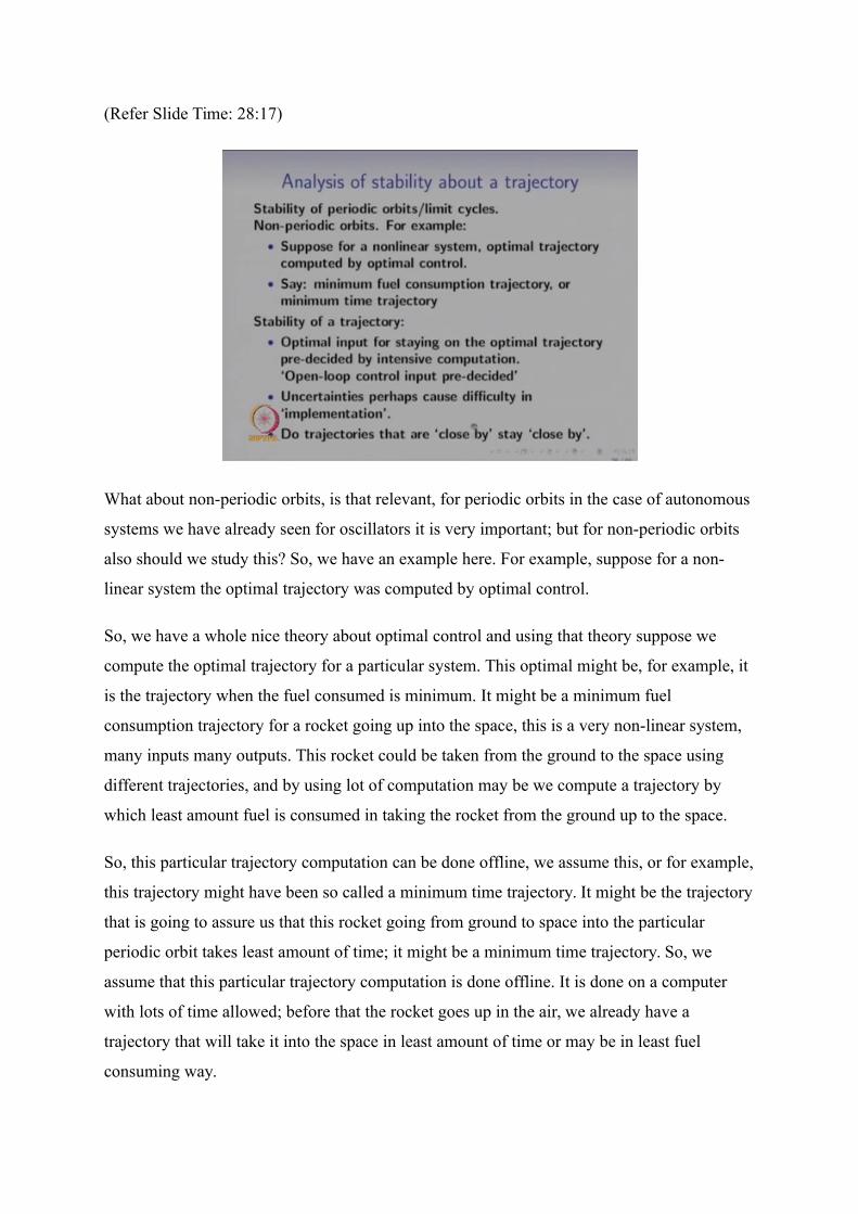
(Refer Slide Time: 28:17)
What about non-periodic orbits, is that relevant, for periodic orbits in the case of autonomous
systems we have already seen for oscillators it is very important; but for non-periodic orbits
also should we study this? So, we have an example here. For example, suppose for a non-
linear system the optimal trajectory was computed by optimal control.
So, we have a whole nice theory about optimal control and using that theory suppose we
compute the optimal trajectory for a particular system. This optimal might be, for example, it
is the trajectory when the fuel consumed is minimum. It might be a minimum fuel
consumption trajectory for a rocket going up into the space, this is a very non-linear system,
many inputs many outputs. This rocket could be taken from the ground to the space using
different trajectories, and by using lot of computation may be we compute a trajectory by
which least amount fuel is consumed in taking the rocket from the ground up to the space.
So, this particular trajectory computation can be done offline, we assume this, or for example,
this trajectory might have been so called a minimum time trajectory. It might be the trajectory
that is going to assure us that this rocket going from ground to space into the particular
periodic orbit takes least amount of time; it might be a minimum time trajectory. So, we
assume that this particular trajectory computation is done offline. It is done on a computer
with lots of time allowed; before that the rocket goes up in the air, we already have a
trajectory that will take it into the space in least amount of time or may be in least fuel
consuming way.
So, this is what is optimal control, and once we have found this optimal trajectory this
optimal input, that is required for staying on the optimal trajectory is pre-decided, for
example, by intensive computation. Now we can ask, given that this particular system is not
going to exactly go along this optimal trajectory… Before we go into that, suppose the open
loop control input is pre-decided, the meaning of that the input that you should give so that
that performance objective is met in optimal way, that input is pre-decided and you just give
this input to the system.
This is same as saying that the control input is open loop. It is open loop control input, and it
is pre-decided, but it is also true that there are various uncertainties in the system. The fuel
may not be of the correct quality that was assumed when you were deciding, when you were
computing the control input. There may be other uncertainties in the space; when the rocket is
going up, it is encountering a situation that is not exactly accounted in the model.
So, because of these uncertainties, it is difficult to implement exactly that particular optimal
trajectory using this pre-decided control input; that time we could ask the question, what if
the trajectories start close by? If the trajectories that are close to this optimal trajectory, do
they stay close by? This is a natural question that arises in this context. If the close by
trajectories do not stay close by, if the optimal trajectory is very good, but the trajectories that
are close to the optimal trajectory perhaps are moving away from the system away from the
optimal trajectory…
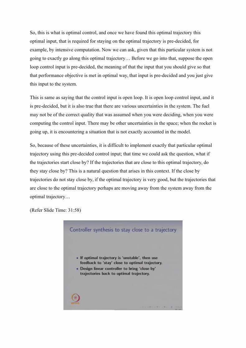
(Refer Slide Time: 31:58)
If that is the case, then we will very soon define that to be unstable optimal trajectory. Then,
perhaps we can use feedback to stay close to this optimal trajectory, what is feedback here?
Our control input was pre-decided, that pre-decided control input is indeed optimal. If all the
modeling has been done to account for all uncertainties, but in the presence of uncertainties
this actual input that we are giving is no longer optimal, because there are some model
uncertainties, which we have not accounted for.
So, perhaps we could use feedback. We could measure the actual sensor values now, and add
the required value to the control input to the pre-decided control input. So, what is this linear
controller supposed to do? It is supposed to…. So, design a linear controller to bring close by
trajectories back to the optimal trajectory. If the trajectories that are close by are not coming
back to the optimal trajectory, then we would like to design a controller that achieves this.
So, as far as this particular problem is concerned, even though the optimal input was pre-
decided, if the trajectory was not the optimal trajectory, then a linear controller suffices for
stabilizing the system back to this optimal trajectory.
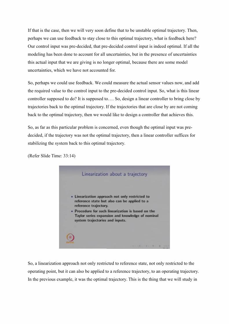
(Refer Slide Time: 33:14)
So, a linearization approach not only restricted to reference state, not only restricted to the
operating point, but it can also be applied to a reference trajectory, to an operating trajectory.
In the previous example, it was the optimal trajectory. This is the thing that we will study in
detail. So, the procedure that we will see very soon is based on a Taylor series expansion and
knowledge of the nominal system trajectories.
So, this reference state, reference trajectory, we will call as nominal state value or nominal
system trajectory. The system trajectory itself has a corresponding nominal input also. What
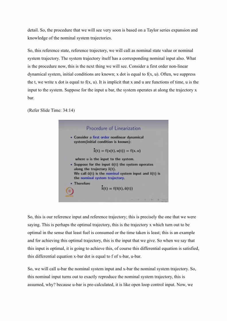
is the procedure now, this is the next thing we will see. Consider a first order non-linear
dynamical system, initial conditions are known; x dot is equal to f(x, u). Often, we suppress
the t, we write x dot is equal to f(x, u). It is implicit that x and u are functions of time, u is the
input to the system. Suppose for the input u bar, the system operates at along the trajectory x
bar.
(Refer Slide Time: 34:14)
So, this is our reference input and reference trajectory; this is precisely the one that we were
saying. This is perhaps the optimal trajectory, this is the trajectory x which turn out to be
optimal in the sense that least fuel is consumed or the time taken is least; this is an example
and for achieving this optimal trajectory, this is the input that we give. So when we say that
this input is optimal, it is going to achieve this, of course this differential equation is satisfied,
this differential equation x-bar dot is equal to f of x-bar, u-bar.
So, we will call u-bar the nominal system input and x-bar the nominal system trajectory. So,
this nominal input turns out to exactly reproduce the nominal system trajectory, this is
assumed, why? because u-bar is pre-calculated, it is like open loop control input. Now, we
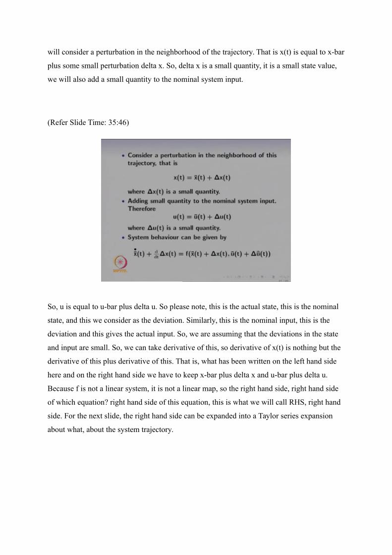
will consider a perturbation in the neighborhood of the trajectory. That is x(t) is equal to x-bar
plus some small perturbation delta x. So, delta x is a small quantity, it is a small state value,
we will also add a small quantity to the nominal system input.
(Refer Slide Time: 35:46)
So, u is equal to u-bar plus delta u. So please note, this is the actual state, this is the nominal
state, and this we consider as the deviation. Similarly, this is the nominal input, this is the
deviation and this gives the actual input. So, we are assuming that the deviations in the state
and input are small. So, we can take derivative of this, so derivative of x(t) is nothing but the
derivative of this plus derivative of this. That is, what has been written on the left hand side
here and on the right hand side we have to keep x-bar plus delta x and u-bar plus delta u.
Because f is not a linear system, it is not a linear map, so the right hand side, right hand side
of which equation? right hand side of this equation, this is what we will call RHS, right hand
side. For the next slide, the right hand side can be expanded into a Taylor series expansion
about what, about the system trajectory.
(Refer Slide Time: 37:05)
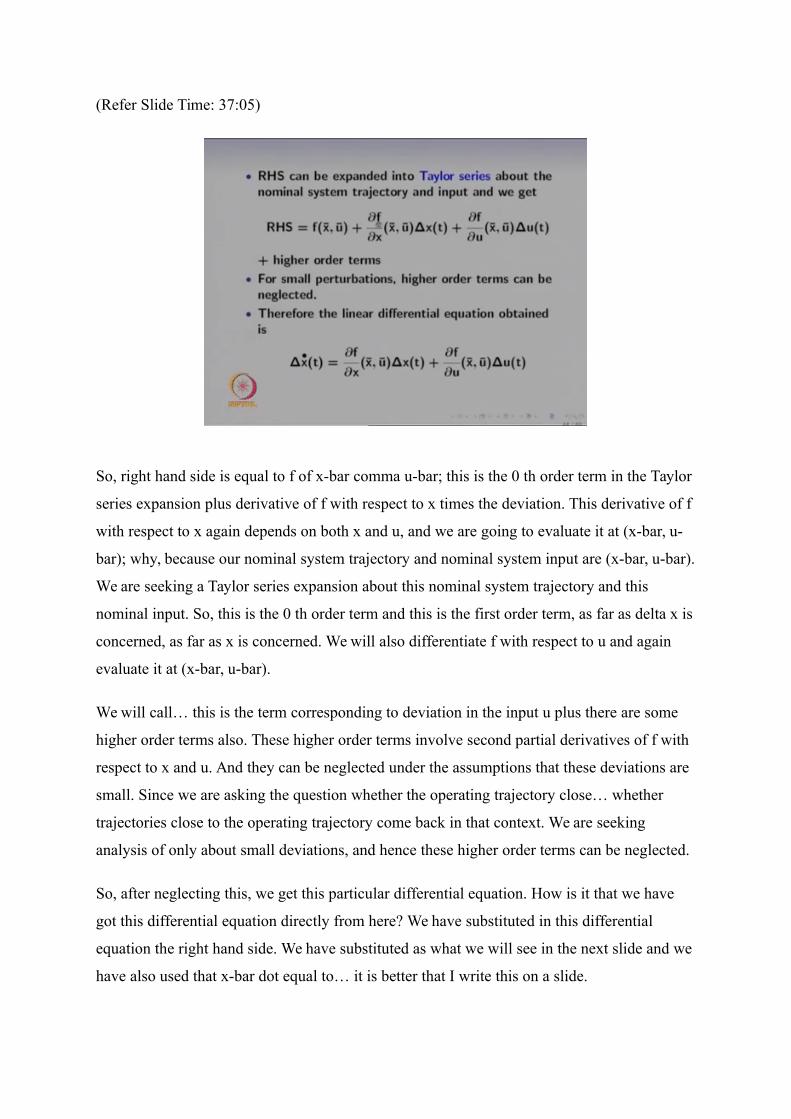
So, right hand side is equal to f of x-bar comma u-bar; this is the 0 th order term in the Taylor
series expansion plus derivative of f with respect to x times the deviation. This derivative of f
with respect to x again depends on both x and u, and we are going to evaluate it at (x-bar, u-
bar); why, because our nominal system trajectory and nominal system input are (x-bar, u-bar).
We are seeking a Taylor series expansion about this nominal system trajectory and this
nominal input. So, this is the 0 th order term and this is the first order term, as far as delta x is
concerned, as far as x is concerned. We will also differentiate f with respect to u and again
evaluate it at (x-bar, u-bar).
We will call… this is the term corresponding to deviation in the input u plus there are some
higher order terms also. These higher order terms involve second partial derivatives of f with
respect to x and u. And they can be neglected under the assumptions that these deviations are
small. Since we are asking the question whether the operating trajectory close… whether
trajectories close to the operating trajectory come back in that context. We are seeking
analysis of only about small deviations, and hence these higher order terms can be neglected.
So, after neglecting this, we get this particular differential equation. How is it that we have
got this differential equation directly from here? We have substituted in this differential
equation the right hand side. We have substituted as what we will see in the next slide and we
have also used that x-bar dot equal to… it is better that I write this on a slide.
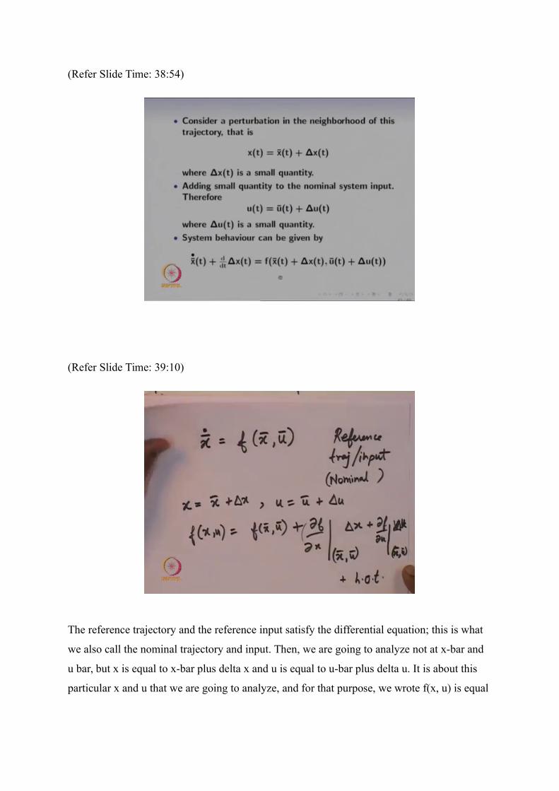
(Refer Slide Time: 38:54)
(Refer Slide Time: 39:10)
The reference trajectory and the reference input satisfy the differential equation; this is what
we also call the nominal trajectory and input. Then, we are going to analyze not at x-bar and
u bar, but x is equal to x-bar plus delta x and u is equal to u-bar plus delta u. It is about this
particular x and u that we are going to analyze, and for that purpose, we wrote f(x, u) is equal
to f(x-bar, u-bar) plus (del f / del x) evaluated at (x-bar, u-bar) times delta x plus (del f / del u)
times delta u. This again evaluated at (x-bar, u-bar).
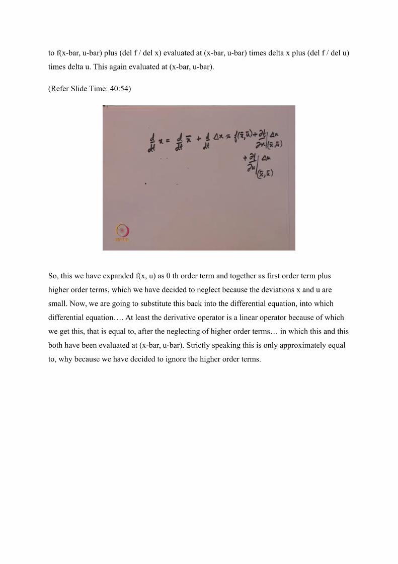
(Refer Slide Time: 40:54)
So, this we have expanded f(x, u) as 0 th order term and together as first order term plus
higher order terms, which we have decided to neglect because the deviations x and u are
small. Now, we are going to substitute this back into the differential equation, into which
differential equation…. At least the derivative operator is a linear operator because of which
we get this, that is equal to, after the neglecting of higher order terms… in which this and this
both have been evaluated at (x-bar, u-bar). Strictly speaking this is only approximately equal
to, why because we have decided to ignore the higher order terms.
(Refer Slide Time: 42:06)
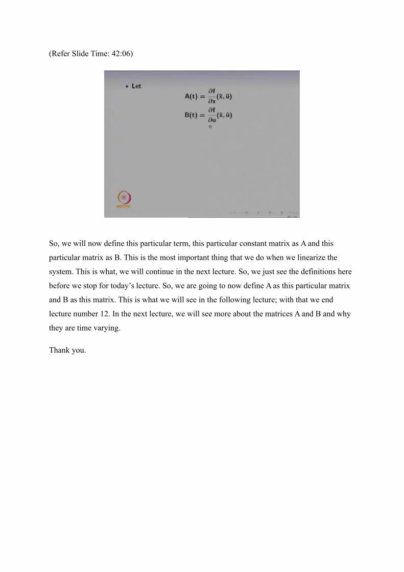
So, we will now define this particular term, this particular constant matrix as A and this
particular matrix as B. This is the most important thing that we do when we linearize the
system. This is what, we will continue in the next lecture. So, we just see the definitions here
before we stop for today’s lecture. So, we are going to now define A as this particular matrix
and B as this matrix. This is what we will see in the following lecture; with that we end
lecture number 12. In the next lecture, we will see more about the matrices A and B and why
they are time varying.
Thank you.
![lec12 [호환 모드] - Sangji Universitycompiler.sangji.ac.kr/lecture/java/2008_1/lec12.pdf · 2019. 2. 14. · Microsoft PowerPoint - lec12 [호환 모드] Author: Main Created](https://img.pdfslide.net/doc/110x75/60bbcfc76d94d3477c546d23/lec12-eeoe-sangji-2019-2-14-microsoft-powerpoint-lec12-.jpg)