Nonlinear Dynamics in Financial Markets: Evidence and ...dah7/faj1995.pdf · Nonlinear Dynamics in Financial Markets: Evidence and Implications by David A. Hsieh Fuqua School of Business

Nonlinear Dynamics in Financial Markets:Evidence and Implications

by

David A. HsiehFuqua School of Business

Duke University

May 1995

This paper was presented at the Institute for Quantitative Research inFinance, October 2-5, 1994.

Abstract

Daily asset returns exhibit two key statistical properties. Returns arenot autocorrelated. But the absolute value of returns are stronglyautocorrelated. Nonlinear processes can generate this type of behavior, whilelinear processes cannot. This paper investigates two types of nonlinearprocesses. Additively nonlinear processes are consistent with the view thatexpected returns are time varying. While much effort has been applied tomodeling expected returns, there has been little evidence to support the viewthat time varying expected returns can account for the strong nonlinearity inthe observed returns data. Multiplicatively nonlinear models are consistentwith the view that expected volatilities are time varying. Evidence fromprice changes as well as options implied volatilities show that volatility istime varying and mean reverting. In fact, multiplicatively nonlinear modelshave been able to explain a great deal of the nonlinearity in asset returns. Thus, it is possible to forecast future volatility, even though it isdifficult to forecast the direction of price changes. This has importantimplications for short term financial risk management.

-1-

Daily price changes for a large number of assets exhibit two key

statistical features. There is very little autocorrelation in price changes,

but there is strong autocorrelation in the absolute value of price changes.

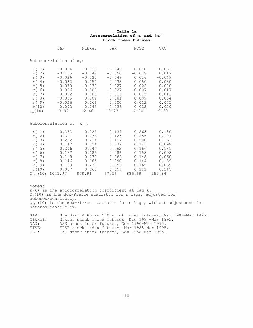
Evidence is provided in Table 1 (1a through 1h). Table 1a uses stock index

futures prices for the S&P, Nikkei, DAX, FTSE, and CAC.

Notationally, let Pt be the price of an asset at date t. Define

xt = ln[Pt/Pt-1]

as the continuous rate of change between the price at dates t-1 and t. The

top panel of Table 1a provides the first ten autocorrelation coefficients of

xt and the Box-Pierce test for all these coefficients to be zero. It is clear

that the autocorrelation coefficients of xt are not different from zero. This

is in agreement with the evidence in the literature. What is striking,

however, is that the autocorrelation coefficients of |xt| are much larger in

the bottom panel of Table 1a. Most of the first order autocorrelation

coefficients are larger than 0.10, and quite a few are larger than 0.20.

These magnitudes are substantial, indicating that the log price differences

are definitely not random. Specifically, a time series is 'random' if each

number is not predictable based on preceding numbers and all numbers have the

same statistical distribution. The precise statistical term for a random

time series is that its numbers are 'independent and identically

distribution.'

The lack of autocorrelation in xt and the large autocorrelation in |xt|

are characteristic of high frequency (e.g. weekly, daily, hourly) data in

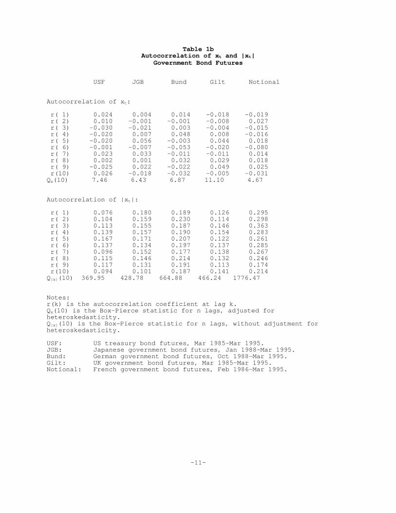
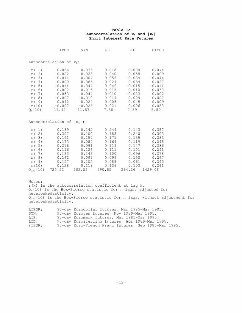
asset markets. They show up strongly in daily price changes of government

bond futures (Table 1b), short interest rate futures (Table 1c), currency

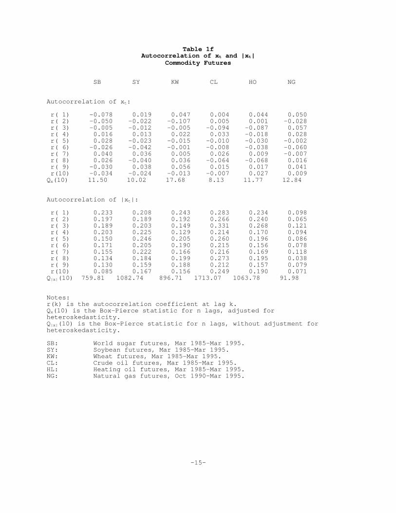
futures (Table 1d), and commodity futures (Table 1e through 1h). This finding

is not sensitive to the sampling period. This paper focuses on the

characterization of these two features, and ignores other well known

characteristics of high frequency data, such as the leptokurtic distribution

of returns.

-2-

Explanations of Non-Random Behavior

There are several competing explanations for the non-random behavior of

asset price changes. In the first place, structural changes or regime changes

in the economy can affect prices behavior in asset markets. A frequently

cited example is the increase in the variance of interest rates between 1979

and 1981, which has been attributed to the change in the Federal Reserve

policy from targeting interest rates to money supplies. This nonstationarity

hypothesis is most persuasive for data spanning long periods of time (e.g.

annual data over many decades), since the underlying structure of the economy

is unlikely to remain constant. But it is not an appealing explanation of the

non-random behavior of asset returns in Table 1. The reason is that non-

random behavior of asset returns is most pronounced in high frequency (i.e.

weekly, daily, or hourly frequencies) data. As the sampling interval is

lengthened to a monthly or quarterly frequency, the autocorrelation of the

absolute value of price changes declines. This is not consistent with

structural change hypothesis. Furthermore, if the structure of the economy

indeed changes at the rate of daily frequencies, it would be impossible to

study the economy statistically, since most economic time series are available

only at monthly or quarterly frequencies.

An alternative to the nonstationarity hypothesis is that the non-random

behavior is an intrinsic part of the dynamics of asset prices. Most of the

past literature on the empirical behavior of price changes have focused on

linear time series models, such as autoregressive-moving average (ARMA)

models. The evidence in Table 1 show that xt is not linear. No linear model

can produce xt which is not autocorrelated but |xt| is autocorrelated. This

leads naturally to nonlinear time series models for xt.

Theoretically, there is good reason for believing that xt is nonlinear.

Modern finance theory suggests that the current price of an asset, Pt, is the

expected discounted value of future payoffs:

Pt = E[ mt,t+1 (Dt+1 + Pt+1) | It].

In this fundamental pricing equation, Dt+1 is the net cash flow generated by

-3-

holding the asset between period t and t+1, and mt,t+1 is a discount factor.

The expectation E[] is taken conditional on the information available at

period t, It. Any asset pricing theory must specify the information set It

and the discount factor mt,t+1. In a typical asset pricing model, such as the

consumption capital asset pricing model, mt,t+1 is the ratio of the marginal

utility of consumption between time t+1 and time t. The asset payoff

(Dt+1+Pt+1) affects the amount of consumption at time t+1, and therefore the

discount factor mt,t+1, so that the pricing equation is a nonlinear stochastic

difference equation, for which there is no general solution available. One

thing, however, is clear. It is very likely that the asset price Pt which

solves the pricing equation will be a nonlinear rather than a linear

stochastic process. Thus the logarithm of price changes (xt=ln[Pt/Pt-1]) is

also likely to be a nonlinear stochastic process.

Empirically, the world of nonlinear processes is vastly richer than the

world of linear processes. Nonlinear processes can generate much more

interesting dynamics than linear processes. Specifically, quite a few

nonlinear processes can generate xt which has no autocorrelation but |xt| has

strong autocorrelation. But a strict discipline must be followed when fitting

nonlinear models to data. There are so many nonlinear processes that it is

very easy to overfit the data. This paper will adhere to the principle of

parsimony --- simple models are preferred to complex models. Two classes of

simple nonlinear stochastic models will be examined: additive and

multiplicative models.

Additively Nonlinear Models

Suppose xt is generated by the following model:

xt = F(It-1) + et,

where et is random, with mean zero and finite variance, and It-1 is the

information available at time t-1. For the purposes of this paper, It-1

consists of the past history of xt-1 and et-1. The function F() is the

conditional mean function, which gives expected return of the asset between

-4-

time t-1 and t using the information in It-1. F() cannot be linear. If it

were, xt would exhibit serial correlation. Such a model is called an

additively nonlinear model, because the error term et is added to the

nonlinear function F(). If price changes are generated by such a model, it

means that most of the nonlinear dynamics are coming from changes in expected

returns.

In the time series literature, there are many examples of additively

nonlinear models: the nonlinear moving average model of Robinson (1977), the

bilinear model of Granger and Anderson (1978), and the threshold

autoregressive model of Tong and Lim (1980). In addition, deterministic chaos

(e.g. the pseudo-random number generators used in most computer simulations)

is a special case in which the noise term et vanishes.

If F() is known, the direction of price change is forecastable. This

has led to much excitement in the finance community. Since F() is unknown,

nonparametric methods (e.g. kernels, neural nets, nearest neighbors, and

series expansions) have been used to estimate F(). The results thus far have

proved disappointing. White (1988), Diebold and Nason (1990), Hsieh (1991,

1993a and 1993b), among others, have used various nonparametric methods to

estimate the conditional mean function for stocks and foreign currencies. The

out-of-sample forecasts perform uniformly worse than the naive model that

prices follow a random walk.

The failure to find a statistically significant conditional mean

function implies that the size and variation of the expected return of holding

assets over one trading day is quite small relative to the magnitude of the

observed price changes. This is not a surprising result. Over long periods

of time, stock returns have averaged on the order of 10% per annum with a

volatility of 20% per annum, which translates to an average return of 0.04%

and a volatility of 1.26% per trading day. The average returns of the bonds,

currencies, and commodities, are typically even small. The strong evidence of

non-random behavior of asset returns is unlikely to be caused by the variation

of expected returns.

-5-

Multiplicatively Nonlinear Models

Suppose xt is obtained by the following model:

xt = G(It-1)� et,

where et is random, with mean zero and finite variance σ2. The function G()

is known as the conditional variance function, and must be positive. The

quantity G(It-1)σ2 can be interpreted as the expected variance of xt based on

information at time t-1. The expected value of xt is zero. Such a model is

called a multiplicatively nonlinear model, because the error term et is

multiplied to the function G(). If price changes are generated by such a

model, it means that most of the nonlinear dynamics are coming from changes in

expected variance.

Examples of multiplicatively nonlinear models are the autoregressive

conditional heteroskedasticity (ARCH) model of Engle (1982) and its

generalized version (GARCH) of Bollerslev (1986). The ARCH-type models have

gained great popularity in the empirical finance literature, as measured by

the number of articles surveyed by Bollerslev, Chow, and Kroner (1992). This

is due to the fact that ARCH-type models have been able to fit the

nonlinearity in asset returns, in the following sense. After an ARCH-type

model is estimated, it provides an estimate of the daily volatility, which can

be used to standardize the return series. The resulting series typical

exhibit little remaining nonlinearity.

In the past, researchers have discovered evidence of volatility changes

at annual and monthly frequencies. See, for example, Officer (1973) and

French, Schwert, and Stambaugh (1987). The evidence now indicate that

volatility changes occur even at daily frequencies. The time-varying nature

of volatility is corroborated by the implied volatilities of options, which

can fluctuate quite a bit from day to day.

The Dynamics of Volatility

-6-

In order to assess the implication of volatility changes on the

application of finance theory, it is important to document the time series

properties of volatility. As early as Mandelbrot (1963), researchers have

known that asset returns exhibit volatility clustering. If the volatility is

high one period, it tends to remain high the next period. If volatility is

low one day, it tends to remain low the next day.

A second key feature of volatility is that it is strongly mean

reverting. This is confirmed in Hsieh (1994), who uses both price based and

option based information to measure volatility, and finds that it is mean

reverting. This observation is further confirmed by the behavior of the term

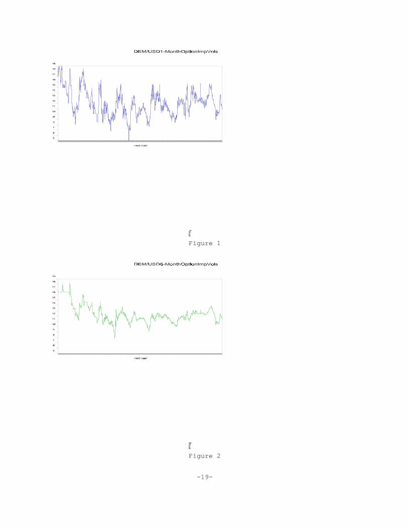
structure of implied volatilities. Figures 1 and 2 are the implied

volatilities of over-the-counter 1- and 6- month options on the US

Dollar/German Mark exchange rate from 1985 to 1992. The 1-month implied

volatility is much more volatile than the 6-month implied volatility, and both

revert to a long run mean around 12%. Moreover, these figures indicate that

volatility tends to revert fairly rapidly back to its long run average.

This last observation directly contradicts the results of most GARCH

models, which have found very high persistence in volatility, to the point

that volatility appears to follow a random walk process. Whether or not

volatility follows a random walk or stationary process is not particularly

relevant for one-day ahead forecasts of volatility, but it is critically

important for multi-day ahead forecasts. This difference is dramatic in the

application to follow.

To capture the mean-reverting behavior of volatility, Hsieh (1993b)

proposed the autoregressive volatility (AV) model:

xt = σt et.

log σt = α + Σ βi log σt-i + νt.

Here, (et, νt) is iid with zero mean (0, 0); et has finite variance σ, νt has

finite variance σ, and et and νt has correlation ρ.

There are two important differences between the AV model and the popular

-7-

GARCH model. In the first place, the AV model has found much less volatility

persistence than the GARCH model. In the second place, the GARCH model have

been estimated using the maximum likelihood method, which requires a specific

distributional assumption on the error terms et. The AV model does not

require any distributional assumptions.

Applications to Financial Risk Management

Once the conditional variance function G() has been estimated, whether

it be the popular GARCH model or the AV model, the conditional distribution of

future values of xt can be obtained using simulation methods. The conditional

distribution can be more informative than the unconditional distribution,

which uses the histogram of xt, thus pretending that returns are random. As

volatility is strongly mean reverting, the conditional distribution should

converge to the unconditional distribution over time. Thus, the conditional

distribution is most useful for assessing the distribution of short term price

changes, probably up to a few weeks.

The conditional distribution of returns can provide useful information

on the market risk of asset and liability positions, as demonstrated in Hsieh

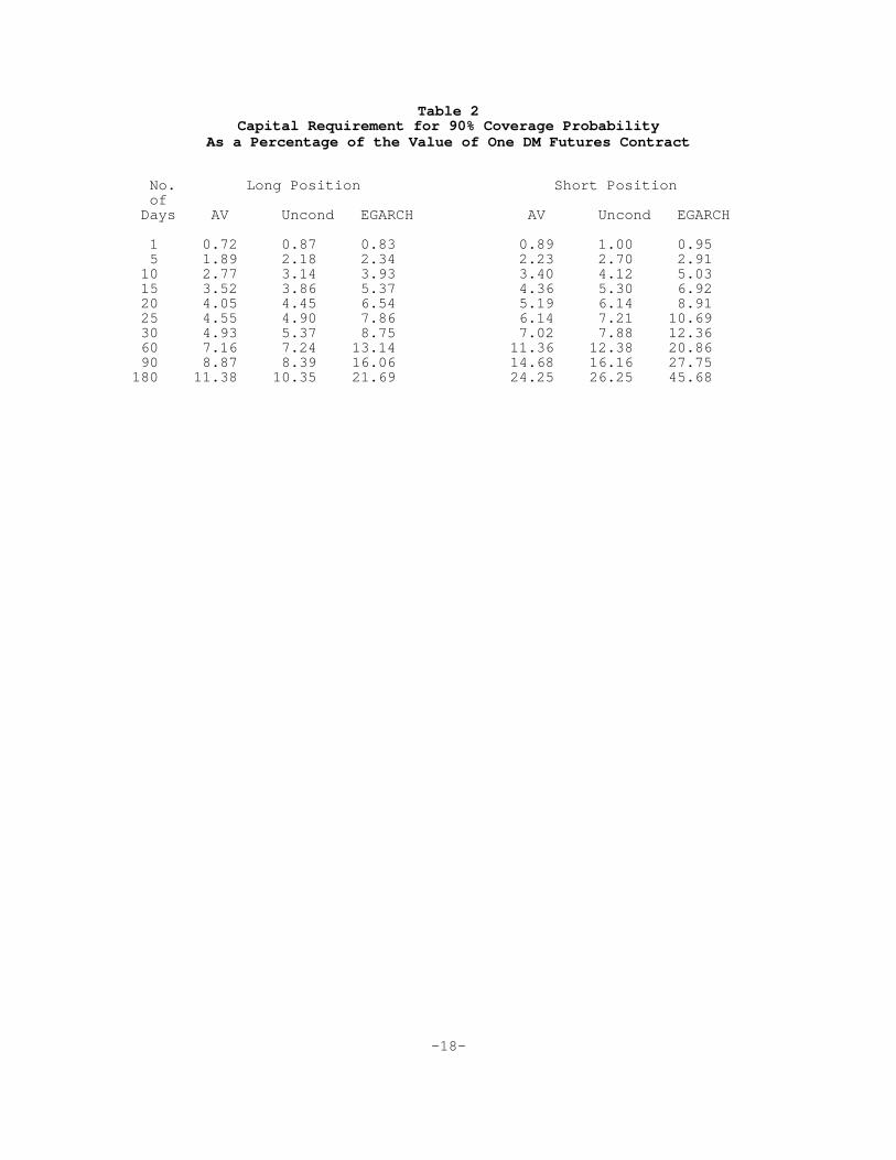
(1993b). Table 2 provides estimates of the capital requirements for 90%

coverage probabilities of one German Mark (DM) futures contract traded on the

Chicago International Money Market over different holding horizons, from 1 to

180 trading days. Suppose the DM futures is trading at $0.40 per DM. One

futures contract is for the delivery of 125,000 DM, or a total value of

$50,000. Based on the AV model, a trader holding a long position for one day

needs 0.72% of the value of the contract, or $360, to cover 90% of all

potential losses the next day. The capital requirement increases to 11.38%,

or $5,690, if the trader wants to cover 90% of all possible losses in the next

180 trading days.

This table compares the difference in capital requirements using the AV

model, the unconditional distribution (which pretends that asset returns are

iid), and a special variant of the GARCH model, called the exponential GARCH

-8-

(EGARCH) model. When the holding period is short, the three models give

reasonably similar results. However, as the holding period increases, the AV

and the unconditional distribution model yield similar results, while the

EGARCH model gives dramatically different results. This is due to the strong

volatility persistence in the EGARCH model.

It is straight forward to extend this risk management analysis from a

single asset to a portfolio of assets, provided that one is willing to make

some assumptions regarding the correlation between asset returns. Such a

portfolio risk management system is discussed in Hsieh (1993c) using the

unconditional distribution for monthly returns. A similar system using the

conditional distribution from the AV model for daily returns can be quite

easily implemented. This portfolio risk assessment system can also serve as

an asset allocation model for short holding periods.

Summary and Conclusion

This paper documents two interesting observations in asset markets, that

daily price changes are not autocorrelated, yet they are non-random. While it

is possible that expected returns are changing over time, they are not able to

explain the strong evidence of non-random behavior. A much more successful

explanation is that volatility is time varying. Volatility tends to cluster,

but it is strongly mean reverting. Conditional variance models, such as ARCH-

type models, can explain a great deal of the non-random behavior in asset

returns. While GARCH and EGARCH models have a tendency to put too much

persistence in volatility, the autoregressive volatility (AV) model is much

better able to capture mean reversion in volatility. These conditional

variance models provide a way to simulate the future distribution of asset

returns, and yield some interesting applications to pricing of options and

financial risk management.

-9-

References:

Bollerslev, T., 1986, Generalized Autoregressive ConditionalHeteroskedasticity, Journal of Econometrics 31, 307-327.

Bollerslev, T., R. Chow, and K. Kroner, 1992, ARCH Modeling in Finance: AReview of the Theory and Empirical Evidence, Journal of Econometrics 52, 5-59.

Diebold, F., and J. Nason, 1990, Nonparametric Exchange Rate Prediction? Journal of International Economics 28, 315-332.

Engle, R., 1982, Autoregressive Conditional Heteroscedasticity With Estimatesof The Variance of U. K. Inflations, Econometrica 50, 987-1007.

French, K., W. Schwert, and R. Stambaugh, 1987, Expected Stock Returns andVolatility, Journal of Financial Economics 19, 3-29.

Granger, C., and A. Andersen, 1978, An Introduction to Bilinear Time SeriesModels (Vanderhoeck & Ruprecht, Göttingen).

Hsieh, D., 1991, Chaos and Nonlinear Dynamics: Application to FinancialMarkets, Journal of Finance 46, 1839-1877.

Hsieh, D., 1993a, Using Non-Linear Models to Search for Risk Premia inCurrency Futures, Journal of International Economics 35, 113-132.

Hsieh, D., 1993b, Implications of Nonlinear Dynamics for Financial RiskManagement, Journal of Financial and Quantitative Analysis 28, 41-64.

Hsieh, D., 1993c, Assessing the Market and Credit Risks of Long-Term InterestRate and Foreign Currency Products, Financial Analysts Journal 49, 75-79.

Hsieh, D., 1994, Estimating the Dynamics of Volatility, unpublishedmanuscript, Duke University.

Mandelbrot, 1963, The Variation of Certain Speculative Prices, Journal ofBusiness 36, 394-419.

Officer, R., 1973, The Variability of the Market Factor of the New York StockExchange, Journal of Business 46, 434-453.

Robinson, P., 1977, The Estimation of a Non-linear Moving Average Model,

Stochastic Processes and Their Applications 5, 81!90.

Tong, H. and K. Lim, 1980, Threshold Autoregression, Limit Cycles, andCyclical Data, Journal of the Royal Statistical Society, series B, 42, 245-292.

White, H., 1988, Economic Prediction Using Neural Networks: the Case of IBMDaily Stock Returns, University of California at San Diego Working Paper.

-10-

Table 1aAutocorrelation of xt and |xt|

Stock Index Futures

S&P Nikkei DAX FTSE CAC

Autocorrelation of xt:

r( 1) -0.014 -0.010 -0.049 0.018 -0.031 r( 2) -0.155 -0.048 -0.050 -0.028 0.017 r( 3) -0.026 -0.020 -0.049 0.026 -0.049 r( 4) -0.032 0.050 0.038 0.050 0.030 r( 5) 0.070 -0.030 0.027 -0.002 -0.020 r( 6) 0.006 -0.009 -0.027 -0.007 -0.017 r( 7) 0.012 0.005 -0.013 0.015 -0.012 r( 8) -0.055 -0.002 -0.081 0.009 -0.034 r( 9) -0.026 0.069 0.020 0.022 0.043 r(10) 0.002 0.043 -0.026 0.023 0.020Qx(10) 3.97 12.46 13.23 4.20 9.30

Autocorrelation of |xt|:

r( 1) 0.272 0.223 0.139 0.268 0.130 r( 2) 0.311 0.234 0.123 0.256 0.107 r( 3) 0.252 0.214 0.117 0.200 0.161 r( 4) 0.147 0.226 0.079 0.143 0.098 r( 5) 0.206 0.244 0.062 0.166 0.181 r( 6) 0.167 0.189 0.086 0.158 0.098 r( 7) 0.119 0.230 0.069 0.148 0.060 r( 8) 0.146 0.165 0.090 0.144 0.139 r( 9) 0.169 0.231 0.053 0.169 0.069 r(10) 0.067 0.165 0.059 0.121 0.145Q|x|(10) 1041.97 878.91 97.29 886.69 259.84

Notes:r(k) is the autocorrelation coefficient at lag k.Qx(10) is the Box-Pierce statistic for n lags, adjusted forheteroskedasticity.Q|x|(10) is the Box-Pierce statistic for n lags, without adjustment forheteroskedasticity.

S&P: Standard & Poors 500 stock index futures, Mar 1985-Mar 1995.Nikkei: Nikkei stock index futures, Dec 1987-Mar 1995.DAX: DAX stock index futures, Nov 1990-Mar 1995.FTSE: FTSE stock index futures, Mar 1985-Mar 1995.CAC: CAC stock index futures, Nov 1988-Mar 1995.

-11-

Table 1bAutocorrelation of xt and |xt|

Government Bond Futures

USF JGB Bund Gilt Notional


r( 1) 0.024 0.004 0.014 -0.018 -0.019 r( 2) 0.010 -0.001 -0.001 -0.008 0.027 r( 3) -0.030 -0.021 0.003 -0.004 -0.015 r( 4) -0.020 0.007 0.048 0.008 -0.016 r( 5) -0.020 0.056 -0.003 0.044 0.018 r( 6) -0.001 -0.007 -0.053 -0.020 -0.080 r( 7) 0.023 0.033 -0.011 -0.011 0.014 r( 8) 0.002 0.001 0.032 0.029 0.018 r( 9) -0.025 0.022 -0.022 0.049 0.025 r(10) 0.026 -0.018 -0.032 -0.005 -0.031Qx(10) 7.46 6.43 6.87 11.10 4.67

Autocorrelation of |xt|: r( 1) 0.076 0.180 0.189 0.126 0.295 r( 2) 0.104 0.159 0.230 0.114 0.298 r( 3) 0.113 0.155 0.187 0.146 0.363 r( 4) 0.139 0.157 0.190 0.154 0.283 r( 5) 0.167 0.171 0.207 0.122 0.261 r( 6) 0.137 0.134 0.197 0.137 0.285 r( 7) 0.096 0.152 0.177 0.138 0.267 r( 8) 0.115 0.146 0.214 0.132 0.246 r( 9) 0.117 0.131 0.191 0.113 0.174 r(10) 0.094 0.101 0.187 0.141 0.214Q|x|(10) 369.95 428.78 664.88 466.24 1776.47


USF: US treasury bond futures, Mar 1985-Mar 1995.JGB: Japanese government bond futures, Jan 1988-Mar 1995.Bund: German government bond futures, Oct 1988-Mar 1995.Gilt: UK government bond futures, Mar 1985-Mar 1995.Notional: French government bond futures, Feb 1986-Mar 1995.

-12-

Table 1cAutocorrelation of xt and |xt|Short Interest Rate Futures

LIBOR SYN LIP LID PIBOR


r( 1) 0.066 0.036 0.018 0.004 0.074 r( 2) 0.022 0.023 -0.040 0.058 0.009 r( 3) -0.011 0.004 0.055 -0.039 -0.044 r( 4) -0.009 0.066 -0.024 0.034 0.027 r( 5) -0.014 0.044 0.046 -0.015 -0.011 r( 6) 0.002 0.013 -0.015 0.010 -0.030 r( 7) 0.053 0.044 0.010 -0.023 0.002 r( 8) -0.007 -0.010 0.014 0.009 0.007 r( 9) -0.042 -0.024 0.005 0.045 -0.009 r(10) -0.007 -0.026 0.021 0.006 0.053Qx(10) 11.42 11.87 7.38 7.59 5.89


r( 1) 0.139 0.142 0.244 0.143 0.357 r( 2) 0.207 0.100 0.183 0.240 0.303 r( 3) 0.191 0.159 0.171 0.135 0.283 r( 4) 0.173 0.084 0.169 0.119 0.298 r( 5) 0.216 0.091 0.119 0.147 0.286 r( 6) 0.116 0.128 0.111 0.101 0.291 r( 7) 0.133 0.143 0.100 0.096 0.278 r( 8) 0.162 0.099 0.099 0.150 0.267 r( 9) 0.157 0.105 0.088 0.061 0.245 r(10) 0.128 0.118 0.136 0.103 0.261Q|x|(10) 723.52 202.52 590.85 294.26 1429.08


LIBOR: 90-day Eurodollar futures, Mar 1985-Mar 1995.SYN: 90-day Euroyen futures, Nov 1989-Mar 1995.LIP: 90-day Euromark futures, Mar 1985-Mar 1995.LID: 90-day Eurosterling futures, Apr 1989-Mar 1995.PIBOR: 90-day Euro-French Franc futures, Sep 1988-Mar 1995.

-13-

Table 1dAutocorrelation of xt and |xt|

Currency Futures

BPF CDF DMF JPF SFF


r( 1) 0.014 0.043 -0.002 -0.013 -0.002 r( 2) 0.012 -0.034 -0.006 -0.008 -0.014 r( 3) -0.011 -0.030 0.005 0.003 0.000 r( 4) 0.006 0.001 0.000 0.004 0.000 r( 5) 0.011 0.013 -0.006 0.011 -0.007 r( 6) -0.003 -0.015 -0.004 -0.020 -0.014 r( 7) -0.031 0.021 -0.020 -0.012 -0.015 r( 8) 0.028 -0.021 0.034 0.028 0.040 r( 9) -0.001 -0.018 0.001 0.014 -0.020 r(10) 0.005 0.000 0.013 0.047 0.030Qx(10) 4.83 10.93 3.91 9.31 7.80

Autocorrelation of |xt|: r( 1) 0.081 0.090 0.052 0.116 0.042 r( 2) 0.094 0.076 0.038 0.058 0.009 r( 3) 0.100 0.091 0.064 0.093 0.060 r( 4) 0.114 0.106 0.060 0.036 0.051 r( 5) 0.084 0.136 0.050 0.080 0.027 r( 6) 0.128 0.086 0.115 0.106 0.104 r( 7) 0.064 0.078 0.064 0.045 0.080 r( 8) 0.058 0.080 0.058 0.052 0.048 r( 9) 0.090 0.103 0.040 0.066 0.007 r(10) 0.111 0.073 0.106 0.025 0.087Q|x|(10) 237.57 231.55 125.94 142.85 94.47


BPF: British Pound futures, Mar 1985-Mar 1995.CDF: Canadian Dollar futures, Mar 1985-Mar 1995.DMF: Deutschemark futures, Mar 1985-Mar 1995.JYF: Japanese Yen futures, Mar 1985-Mar 1995.SFF: Swiss Franc futures, Mar 1985-Mar 1995.

-14-

Table 1eAutocorrelation of xt and |xt|

Commodity Futures

CR CC JO KC PB


r( 1) -0.071 0.000 -0.007 0.012 0.053 r( 2) -0.020 -0.046 -0.027 0.014 0.031 r( 3) -0.048 -0.005 0.036 0.018 0.001 r( 4) 0.043 -0.015 0.051 0.008 0.015 r( 5) 0.002 0.014 0.021 -0.030 -0.005 r( 6) -0.030 -0.009 0.004 -0.037 0.011 r( 7) 0.007 -0.014 0.000 0.000 0.006 r( 8) -0.040 0.005 -0.001 0.040 0.026 r( 9) 0.033 -0.014 0.043 0.010 -0.007 r(10) -0.046 0.017 0.000 0.068 0.031Qx(10) 17.37 7.47 11.26 8.51 12.81


r( 1) 0.164 0.053 0.150 0.191 0.089 r( 2) 0.149 0.030 0.141 0.180 0.050 r( 3) 0.146 0.068 0.139 0.174 0.049 r( 4) 0.172 0.074 0.128 0.150 0.079 r( 5) 0.200 0.074 0.094 0.170 0.067 r( 6) 0.135 0.069 0.089 0.155 0.093 r( 7) 0.129 0.077 0.111 0.173 0.082 r( 8) 0.161 0.072 0.110 0.139 0.063 r( 9) 0.137 0.066 0.128 0.149 0.069 r(10) 0.146 0.109 0.072 0.216 0.043Q|x|(10) 555.80 135.95 373.24 773.86 130.58


CR: CRB index futures, Jun 1986-Mar 1995.CC: Cocoa futures, Mar 1985-Mar 1995.JO: Orange juice futures, Mar 1985-Mar 1995.KC: Coffee futures, Mar 1985-Mar 1995.PB: Pork belly futures, Mar 1985-Mar 1995.

-15-

Table 1fAutocorrelation of xt and |xt|

Commodity Futures

SB SY KW CL HO NG


r( 1) -0.078 0.019 0.047 0.004 0.044 0.050 r( 2) -0.050 -0.022 -0.107 0.005 0.001 -0.028 r( 3) -0.005 -0.012 -0.005 -0.094 -0.087 0.057 r( 4) 0.016 0.013 0.022 0.033 -0.018 0.028 r( 5) 0.028 -0.023 -0.015 -0.010 -0.030 -0.002 r( 6) -0.026 -0.042 -0.001 -0.008 -0.038 -0.060 r( 7) 0.040 0.036 0.005 0.026 0.009 -0.007 r( 8) 0.026 -0.040 0.036 -0.064 -0.068 0.016 r( 9) -0.030 0.038 0.056 0.015 0.017 0.041 r(10) -0.034 -0.024 -0.013 -0.007 0.027 0.009 Qx(10) 11.50 10.02 17.68 8.13 11.77 12.84


r( 1) 0.233 0.208 0.243 0.283 0.234 0.098 r( 2) 0.197 0.189 0.192 0.266 0.240 0.065 r( 3) 0.189 0.203 0.149 0.331 0.268 0.121 r( 4) 0.203 0.225 0.129 0.214 0.170 0.094 r( 5) 0.150 0.246 0.205 0.260 0.196 0.086 r( 6) 0.171 0.205 0.190 0.215 0.156 0.078 r( 7) 0.155 0.222 0.166 0.216 0.169 0.118 r( 8) 0.134 0.184 0.199 0.273 0.195 0.038 r( 9) 0.130 0.159 0.188 0.212 0.157 0.079 r(10) 0.085 0.167 0.156 0.249 0.190 0.071 Q|x|(10) 759.81 1082.74 896.71 1713.07 1063.78 91.98


SB: World sugar futures, Mar 1985-Mar 1995.SY: Soybean futures, Mar 1985-Mar 1995.KW: Wheat futures, Mar 1985-Mar 1995.CL: Crude oil futures, Mar 1985-Mar 1995.HL: Heating oil futures, Mar 1985-Mar 1995.NG: Natural gas futures, Oct 1990-Mar 1995.

-16-

Table 1gAutocorrelation of xt and |xt|

Commodity Futures

HG PL GC SI ALU


r( 1) -0.038 -0.005 -0.065 -0.068 -0.130 r( 2) 0.008 -0.011 -0.022 -0.004 -0.101 r( 3) -0.029 -0.024 -0.021 -0.013 0.021 r( 4) -0.019 -0.007 0.026 0.008 -0.002 r( 5) -0.004 -0.010 0.021 0.003 0.009 r( 6) 0.027 -0.010 -0.044 -0.047 -0.008 r( 7) -0.011 -0.021 0.007 -0.005 0.029 r( 8) -0.030 0.011 0.004 -0.007 -0.003 r( 9) 0.062 -0.015 0.027 0.006 0.010 r(10) 0.034 0.052 0.012 -0.026 -0.031Qx(10) 10.23 7.61 13.73 5.28 21.89


r( 1) 0.123 0.156 0.166 0.197 0.195 r( 2) 0.075 0.123 0.102 0.161 0.196 r( 3) 0.070 0.120 0.123 0.179 0.111 r( 4) 0.077 0.111 0.119 0.137 0.095 r( 5) 0.091 0.144 0.154 0.137 0.069 r( 6) 0.134 0.107 0.117 0.136 0.076 r( 7) 0.088 0.156 0.113 0.108 0.072 r( 8) 0.087 0.153 0.097 0.040 0.084 r( 9) 0.130 0.122 0.099 0.037 0.094 r(10) 0.064 0.146 0.127 0.129 0.141Q|x|(10) 132.03 480.18 404.65 486.40 394.32


HG: Copper futures, Nov 1989-Mar 1995.PL: Platinum futures, Mar 1985-Mar 1995.GC: Gold, London afternoon fixing, Mar 1985-Mar 1995.SI: Silver, Handy Harmon, Mar 1985-Mar 1995.ALU: Aluminum, New York, Mar 1985-Mar 1995.

-17-

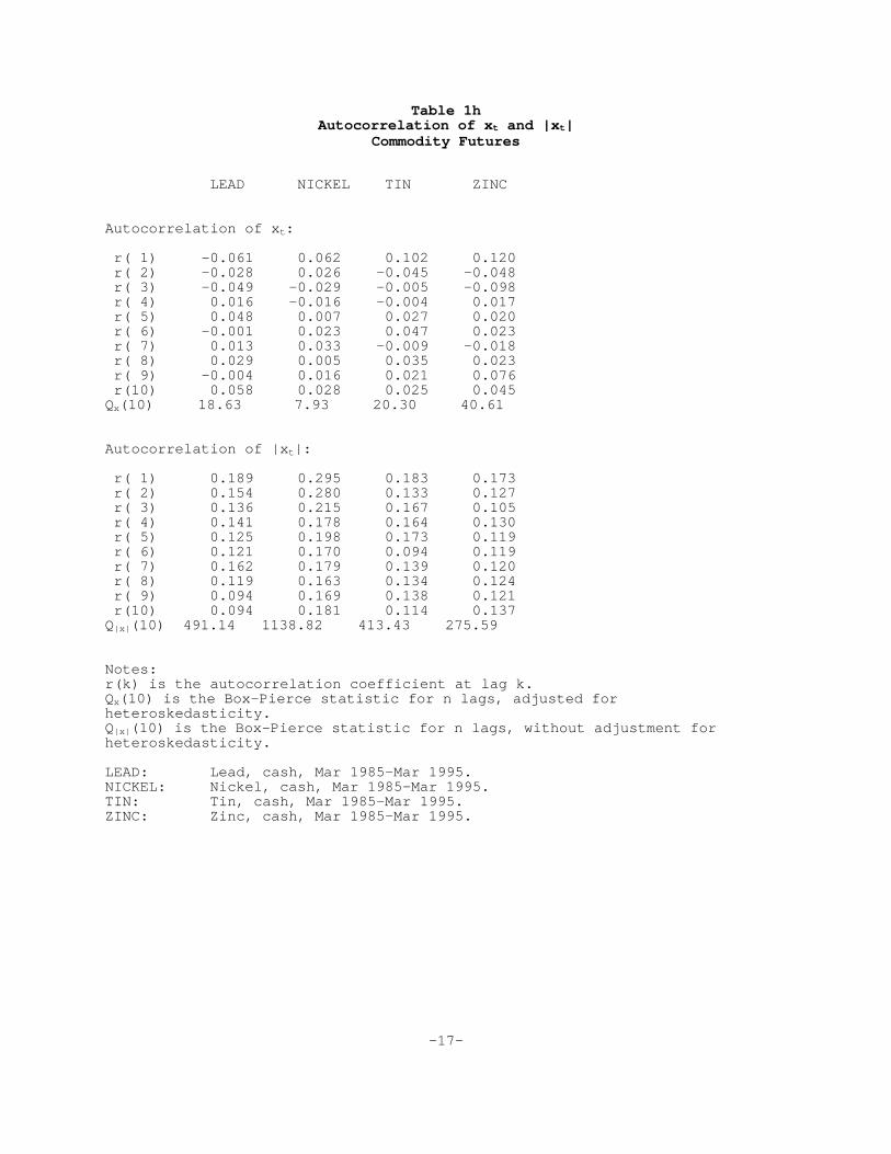
Table 1hAutocorrelation of xt and |xt|

Commodity Futures

LEAD NICKEL TIN ZINC


r( 1) -0.061 0.062 0.102 0.120 r( 2) -0.028 0.026 -0.045 -0.048 r( 3) -0.049 -0.029 -0.005 -0.098 r( 4) 0.016 -0.016 -0.004 0.017 r( 5) 0.048 0.007 0.027 0.020 r( 6) -0.001 0.023 0.047 0.023 r( 7) 0.013 0.033 -0.009 -0.018 r( 8) 0.029 0.005 0.035 0.023 r( 9) -0.004 0.016 0.021 0.076 r(10) 0.058 0.028 0.025 0.045Qx(10) 18.63 7.93 20.30 40.61


r( 1) 0.189 0.295 0.183 0.173 r( 2) 0.154 0.280 0.133 0.127 r( 3) 0.136 0.215 0.167 0.105 r( 4) 0.141 0.178 0.164 0.130 r( 5) 0.125 0.198 0.173 0.119 r( 6) 0.121 0.170 0.094 0.119 r( 7) 0.162 0.179 0.139 0.120 r( 8) 0.119 0.163 0.134 0.124 r( 9) 0.094 0.169 0.138 0.121 r(10) 0.094 0.181 0.114 0.137Q|x|(10) 491.14 1138.82 413.43 275.59


LEAD: Lead, cash, Mar 1985-Mar 1995.NICKEL: Nickel, cash, Mar 1985-Mar 1995.TIN: Tin, cash, Mar 1985-Mar 1995.ZINC: Zinc, cash, Mar 1985-Mar 1995.

-18-

Table 2Capital Requirement for 90% Coverage Probability

As a Percentage of the Value of One DM Futures Contract

No. Long Position Short Position of Days AV Uncond EGARCH AV Uncond EGARCH

1 0.72 0.87 0.83 0.89 1.00 0.95 5 1.89 2.18 2.34 2.23 2.70 2.91 10 2.77 3.14 3.93 3.40 4.12 5.03 15 3.52 3.86 5.37 4.36 5.30 6.92 20 4.05 4.45 6.54 5.19 6.14 8.91 25 4.55 4.90 7.86 6.14 7.21 10.69 30 4.93 5.37 8.75 7.02 7.88 12.36 60 7.16 7.24 13.14 11.36 12.38 20.86 90 8.87 8.39 16.06 14.68 16.16 27.75 180 11.38 10.35 21.69 24.25 26.25 45.68

-19-

Figure 1

Figure 2

Documents

Nonlinear Dynamics in Financial Markets: Evidence and ...dah7/faj1995.pdf · Nonlinear Dynamics in Financial Markets: Evidence and Implications by David A. Hsieh Fuqua School of Business