Embed Size (px)
Citation preview
Nonlinear image processing using artificial neural
networks
Dick de Ridderlowast Robert PW DuinlowastMichael Egmont-Petersendagger
Lucas J van Vlietlowast and Piet W VerbeeklowastlowastPattern Recognition Group Dept of Applied Physics
Delft University of TechnologyLorentzweg 1 2628 CJ Delft The Netherlands
daggerDecision Support Systems GroupInstitute of Information and Computing Sciences Utrecht University
PO box 80089 3508 TB Utrecht The Netherlands
Contents
1 Introduction 211 Image processing 212 Artificial neural networks (ANNs) 313 ANNs for image processing 5
2 Applications of ANNs in image processing 621 Feed-forward ANNs 622 Other ANN types 823 Applications of ANNs 924 Discussion 12
3 Shared weight networks for object recognition 1331 Shared weight networks 1432 Handwritten digit recognition 1833 Discussion 23
4 Feature extraction in shared weight networks 2341 Edge recognition 2442 Two-class handwritten digit classification 3243 Discussion 37
5 Regression networks for image restoration 4451 Kuwahara filtering 4452 Architectures and experiments 4553 Investigating the error 5454 Discussion 55
1
6 Inspection and improvement of regression networks 5561 Edge-favouring sampling 5862 Performance measures for edge-preserving smoothing 5863 Inspection of trained networks 6464 Discussion 67
7 Conclusions 6871 Applicability 7872 Prior knowledge 7973 Interpretability 8074 Conclusions 81
Abstract
Artificial neural networks (ANNs) are very general function approxima-tors which can be trained based on a set of examples Given their generalnature ANNs would seem useful tools for nonlinear image processingThis paper tries to answer the question whether image processing opera-tions can sucessfully be learned by ANNs and if so how prior knowledgecan be used in their design and what can be learned about the problem athand from trained networks After an introduction to ANN types and abrief literature review the paper focuses on two cases supervised classifi-cation ANNs for object recognition and feature extraction and supervisedregression ANNs for image pre-processing A range of experimental re-sults lead to the conclusion that ANNs are mainly applicable to problemsrequiring a nonlinear solution for which there is a clear unequivocal per-formance criterion ie high-level tasks in the image processing chain(such as object recognition) rather than low-level tasks The drawbacksare that prior knowledge cannot easily be used and that interpretation oftrained ANNs is hard
1 Introduction
11 Image processing
Image processing is the field of research concerned with the develop-ment of computer algorithms working on digitised images (eg Pratt 1991Gonzalez and Woods 1992) The range of problems studied in image processingis large encompassing everything from low-level signal enhancement to high-level image understanding In general image processing problems are solved bya chain of tasks This chain shown in figure 1 outlines the possible processingneeded from the initial sensor data to the outcome (eg a classification or ascene description) The pipeline consists of the steps of pre-processing datareduction segmentation object recognition and image understanding In eachstep the input and output data can either be images (pixels) measurementsin images (features) decisions made in previous stages of the chain (labels) oreven object relation information (graphs)
There are many problems in image processing for which good theoreticallyjustifiable solutions exists especially for problems for which linear solutionssuffice For example for pre-processing operations such as image restorationmethods from signal processing such as the Wiener filter can be shown to bethe optimal linear approach However these solutions often only work under
2
Texture segregationColour recognitionClustering
Segmentation
Scene analysisObject arrangement
Objectrecognition
Graph matchingAutomatic thresholding
Optimisation
understandingImage
Template matchingFeatureminusbased recognitionDeblurring
Noise suppressionReconstruction Image enhancement
Edge detectionLandmark extraction
Featureextraction
Preminusprocessing
Figure 1 The image processing chain
ideal circumstances they may be highly computationally intensive (eg whenlarge numbers of linear models have to be applied to approximate a nonlinearmodel) or they may require careful tuning of parameters Where linear modelsare no longer sufficient nonlinear models will have to be used This is still anarea of active research as each problem will require specific nonlinearities to beintroduced That is a designer of an algorithm will have to weigh the differentcriteria and come to a good choice based partly on experience Furthermoremany algorithms quickly become intractable when nonlinearities are introducedProblems further in the image processing chain such object recognition and im-age understanding cannot even (yet) be solved using standard techniques Forexample the task of recognising any of a number of objects against an arbi-trary background calls for human capabilities such as the ability to generaliseassociate etc
All this leads to the idea that nonlinear algorithms that can be trained ratherthan designed might be valuable tools for image processing To explain why abrief introduction into artificial neural networks will be given first
12 Artificial neural networks (ANNs)
In the 1940s psychologists became interested in modelling the human brainThis led to the development of the a model of the neuron as a thresholdedsummation unit (McCulloch and Pitts 1943) They were able to prove that(possibly large) collections of interconnected neuron models neural networkscould in principle perform any computation if the strengths of the interconnec-tions (or weights) were set to proper values In the 1950s neural networks werepicked up by the growing artificial intelligence community
In 1962 a method was proposed to train a subset of a specific class ofnetworks called perceptrons based on examples (Rosenblatt 1962) Percep-trons are networks having neurons grouped in layers with only connectionsbetween neurons in subsequent layers However Rosenblatt could only proveconvergence for single-layer perceptrons Although some training algorithms forlarger neural networks with hard threshold units were proposed (Nilsson 1965)enthusiasm waned after it was shown that many seemingly simple prob-lems were in fact nonlinear and that perceptrons were incapable of solving
3
Classification Regression
UnsupervisedSupervised
Sections III amp IV Sections V amp VI
networksNeural
Figure 2 Adaptive method types discussed in this paper
these (Minsky and Papert 1969)Interest in artificial neural networks (henceforth ldquoANNsrdquo) increased again
in the 1980s after a learning algorithm for multi-layer perceptrons wasproposed the back-propagation rule (Rumelhart et al 1986) This allowednonlinear multi-layer perceptrons to be trained as well However feed-forward networks were not the only type of ANN under research Inthe 1970s and 1980s a number of different biologically inspired learningsystems were proposed Among the most influential were the Hopfieldnetwork (Hopfield 1982 Hopfield and Tank 1985) Kohonenrsquos self-organisingmap (Kohonen 1995) the Boltzmann machine (Hinton et al 1984) and theNeocognitron (Fukushima and Miyake 1982)
The definition of what exactly constitutes an ANN is rather vague In generalit would at least require a system to
bull consist of (a large number of) identical simple processing units
bull have interconnections between these units
bull posess tunable parameters (weights) which define the systemrsquos functionand
bull lack a supervisor which tunes each individual weight
However not all systems that are called neural networks fit this descriptionThere are many possible taxonomies of ANNs Here we concentrate on learn-
ing and functionality rather than on biological plausibility topology etc Fig-ure 2 shows the main subdivision of interest supervised versus unsupervisedlearning Although much interesting work has been done in unsupervised learn-ing for image processing (see eg Egmont-Petersen et al 2002) we will restrictourselves to supervised learning in this paper In supervised learning there is adata set L containing samples in x isin Rd where d is the number of dimensionsof the data set For each x a dependent variable y isin Rm has to be supplied aswell The goal of a regression method is then to predict this dependent variablebased on x Classification can be seen as a special case of regression in whichonly a single variable t isin N is to be predicted the label of the class to whichthe sample x belongs
In section 2 the application of ANNs to these tasks will be discussed in moredetail
4
13 ANNs for image processing
As was discussed above dealing with nonlinearity is still a major problem inimage processing ANNs might be very useful tools for nonlinear image process-ing
bull instead of designing an algorithm one could construct an example dataset and an error criterion and train ANNs to perform the desired input-output mapping
bull the network input can consist of pixels or measurements in images theoutput can contain pixels decisions labels etc as long as these canbe coded numerically ndash no assumptions are made This means adaptivemethods can perform several steps in the image processing chain at once
bull ANNs can be highly nonlinear the amount of nonlinearity can be influ-enced by design but also depends on the training data (Raudys 1998aRaudys 1998b)
bull some types of ANN have been shown to be universal classification or re-gression techniques (Funahashi 1989 Hornik et al 1989)
However it is not to be expected that application of any ANN to any givenproblem will give satisfactory results This paper therefore studies the possi-bilities and limitations of the ANN approach to image processing The mainquestions it tries to answer are
bull Can image processing operations be learned by ANNs To what extent canANNs solve problems that are hard to solve using standard techniquesIs nonlinearity really a bonus
bull How can prior knowledge be used if available Can for example the factthat neighbouring pixels are highly correlated be used in ANN design ortraining
bull What can be learned from ANNs trained to solve image processing prob-lems If one finds an ANN to solve a certain problem can one learn howthe problem should be approached using standard techniques Can oneextract knowledge from the solution
Especially the last question is intriguing One of the main drawbacks of manyANNs is their black-box character which seriously impedes their application insystems in which insight in the solution is an important factor eg medicalsystems If a developer can learn how to solve a problem by analysing thesolution found by an ANN this solution may be made more explicit
It is to be expected that for different ANN types the answers to these ques-tions will be different This paper is therefore laid out as follows
bull first in section 2 a brief literature overview of applications of ANNs toimage processing is given
bull in sections 3 and 4 classification ANNs are applied to object recognitionand feature extraction
5
Bias b2 Bias b3
Class 1
Class 2
Class 3
Input 2
Input 1
Input m
w21 w32
Figure 3 A feed-forward ANN for a three-class classification problem Thecenter layer is called the hidden layer
bull in sections 5 and 6 regression ANNs are investigated as nonlinear imagefilters
These methods are not only applied to real-life problems but also studied toanswer the questions outlined above In none of the applications the goal is toobtain better performance than using traditional methods instead the goal isto find the conditions under which ANNs could be applied
2 Applications of ANNs in image processing
This section will first discuss the most widely used type of ANN the feed-forward ANN and its use as a classifier or regressor Afterwards a brief reviewof applications of ANNs to image processing problems will be given
21 Feed-forward ANNs
This paper will deal mostly with feed-forward ANNs (Hertz et al 1991Haykin 1994) (or multi-layer perceptrons MLPs) They consist of intercon-nected layers of processing units or neurons see figure 3 In this figure thenotation of weights and biases follows (Hertz et al 1991) weights of connec-tions between layer p and layer q are indicated by wqp the bias input andoutput vectors of layer p are indicated by bp Ip and Op respectively Basicallya feed-forward ANN is a (highly) parameterised adaptable vector functionwhich may be trained to perform classification or regression tasks A classifica-tion feed-forward ANN performs the mapping
N Rd rarr 〈rmin rmax〉m (1)
with d the dimension of the input (feature) space m the number of classesto distinguish and 〈rmin rmax〉 the range of each output unit The following
6
feed-forward ANN with one hidden layer can realise such a mapping
N(x WB) = f(w32Tf(w21T
xminus b2)minus b3) (2)
W is the weight set containing the weight matrix connecting the input layerwith the hidden layer (w21) and the vector connecting the hidden layer withthe output layer (w32) B (b2 and b3) contains the bias terms of the hiddenand output nodes respectively The function f(a) is the nonlinear activationfunction with range 〈rmin rmax〉 operating on each element of its input vectorUsually one uses either the sigmoid function f(a) = 1
1+eminusa with the range〈rmin = 0 rmax = 1〉 the double sigmoid function f(a) = 2
1+eminusa minus 1 or the hy-perbolic tangent function f(a) = tanh(a) both with range 〈rmin = minus1 rmax =1〉
211 Classification
To perform classification an ANN should compute the posterior probabilitiesof given vectors x P (ωj |x) where ωj is the label of class j j = 1 m Clas-sification is then performed by assigning an incoming sample x to that classfor which this probability is highest A feed-forward ANN can be trained ina supervised way to perform classification when presented with a number oftraining samples L = (x t) with tl high (eg 09) indicating the correctclass membership and tk low (eg 01) forallk 6= l The training algorithm forexample back-propagation (Rumelhart et al 1986) or conjugate gradient de-scent (Shewchuk 1994) tries to minimise the mean squared error (MSE) func-tion
E(WB) =1
2|L|sum
(xiti)isinL
csumk=1
(N(xi WB)k minus tik)2 (3)
by adjusting the weights and bias terms For more details ontraining feed-forward ANNs see eg (Hertz et al 1991 Haykin 1994)(Richard and Lippmann 1991) showed that feed-forward ANNs when providedwith enough nodes in the hidden layer an infinitely large training set and 0-1training targets approximate the Bayes posterior probabilities
P (ωj |x) =P (ωj)p(x|ωj)
p(x) j = 1 m (4)
with P (ωj) the prior probability of class j p(x|ωj) the class-conditional proba-bility density function of class j and p(x) the probability of observing x
212 Regression
Feed-forward ANNs can also be trained to perform nonlinear multivariate re-gression where a vector of real numbers should be predicted
R Rd rarr Rm (5)
with m the dimensionality of the output vector The following feed-forwardANN with one hidden layer can realise such a mapping
R(x WB) = w32Tf(w21T
xminus b2)minus b3 (6)
7
The only difference between classification and regression ANNs is that in thelatter application of the activation function is omitted in the last layer allowingthe prediction of values in Rm However this last layer activation function canbe applied when the desired output range is limited The desired output of aregression ANN is the conditional mean (assuming continuous input x)
E(y|x) =int
Rm
yp(y|x)dy (7)
A training set L containing known pairs of input and output values (xy) isused to adjust the weights and bias terms such that the mean squared errorbetween the predicted value and the desired value
E(WB) =1
2|L|sum
(xiyi)isinL
msumk=1
(R(xi WB)k minus yik)2 (8)
(or the prediction error) is minimisedSeveral authors showed that under some assumptions regression feed-forward
ANNs are universal approximators If the number of hidden nodes is allowedto increase towards infinity they can approximate any continuous function witharbitrary precision (Funahashi 1989 Hornik et al 1989) When a feed-forwardANN is trained to approximate a discontinuous function two hidden layers aresufficient for obtaining an arbitrary precision (Sontag 1992)
However this does not make feed-forward ANNs perfect classification or re-gression machines There are a number of problems
bull there is no theoretically sound way of choosing the optimal ANN ar-chitecture or number of parameters This is called the bias-variancedilemma (Geman et al 1992) for a given data set size the more pa-rameters an ANN has the better it can approximate the function to belearned at the same time the ANN becomes more and more susceptibleto overtraining ie adapting itself completely to the available data andlosing generalisation
bull for a given architecture learning algorithms often end up in a local mini-mum of the error measure E instead of a global minimum1
bull they are non-parametric ie they do not specify a model and are less opento explanation This is sometimes referred to as the black box problemAlthough some work has been done in trying to extract rules from trainedANNs (Tickle et al 1998) in general it is still impossible to specify ex-actly how an ANN performs its function For a rather polemic discussionon this topic see the excellent paper by Green (Green 1998))
22 Other ANN types
Two other major ANN types are1Although current evidence suggests this is actually one of the features that makes feed-
forward ANNs powerful the limitations the learning algorithm imposes actually manage thebias-variance problem (Raudys 1998a Raudys 1998b)
8
bull the self-organising map (SOM Kohonen 1995 also called topologicalmap) is a kind of vector quantisation method SOMs are trained in an un-supervised manner with the goal of projecting similar d-dimensional inputvectors to neighbouring positions (nodes) on an m-dimensional discretelattice Training is called competitive at each time step one winningnode gets updated along with some nodes in its neighbourhood Aftertraining the input space is subdivided into q regions corresponding tothe q nodes in the map An important application of SOMs in image pro-cessing is therefore unsupervised cluster analysis eg for segmentation
bull the Hopfield ANN (HNN Hopfield 1982) consists of a number of fullyinterconnected binary nodes which at each given time represent a certainstate Connected to a state is an energy level the output of the HNNrsquosenergy function given the state The HNN maps binary input sets onbinary output sets it is initialised with a binary pattern and by iteratingan update equation it changes its state until the energy level is minimisedHNNs are not thus trained in the same way that feed-forward ANNs andSOMs are the weights are usually set manually Instead the power ofthe HNN lies in running it
Given a rule for setting the weights based on a training set of binary pat-terns the HNN can serve as an auto-associative memory (given a partiallycompleted pattern it will find the nearest matching pattern in the train-ing set) Another application of HNNs which is quite interesting in animage processing setting (Poggio and Koch 1985) is finding the solutionto nonlinear optimisation problems This entails mapping a function tobe minimised on the HNNrsquos energy function However the application ofthis approach is limited in the sense that the HNN minimises just one en-ergy function whereas most problems are more complex in the sense thatthe minimisation is subject to a number of constraints Encoding theseconstraints into the energy function takes away much of the power of themethod by calling for a manual setting of various parameters which againinfluence the outcome
23 Applications of ANNs
Image processing literature contains numerous applications of the above types ofANNs and various other more specialised models Below we will give a broadoverview of these applications without going into specific ones Furthermore wewill only discuss application of ANNs directly to pixel data (ie not to derivedfeatures) For a more detailed overview see eg Egmont-Petersen et al 2002
231 Pre-processing
Pre-processing an image can consist of image reconstruction (building up animage from a number of indirect sensor measurements) andor image restoration(removing abberations introduced by the sensor including noise) To performpre-processing ANNs have been applied in the following ways
bull optimisation of an objective function specified by a traditional pre-processing approach
9
bull approximation of a mathematical transformation used in reconstructionby regression
bull general regressionclassification usually directly on pixel data (neighbour-hood input pixel output)
To solve the first type of problem HNNs can be used for the optimisationinvolved in traditional methods However mapping the actual problem to theenergy function of the HNN can be difficult Occasionally the original problemwill have to be modified Having managed to map the problem appropriatelythe HNN can be a useful tool in image pre-processing although convergence toa good result is not guaranteed
For image reconstruction regression (feed-forward) ANNs can be applied Al-though some succesful applications are reported in literature it would seem thatthese applications call for more traditional mathematical techniques because aguaranteed performance of the reconstruction algorithm is essential
Regression or classification ANNs can also be trained to perform imagerestoration directly on pixel data In literature for a large number of appli-cations non-adaptive ANNs were used Where ANNs are adaptive their archi-tectures usually differ much from those of the standard ANNs prior knowledgeabout the problem is used to design them (eg in cellular neural networksCNNs) This indicates that the fast parallel operation of ANNs and the easewith which they can be embedded in hardware can be important factors inchoosing for a neural implementation of a certain pre-processing operationHowever their ability to learn from data is apparently of less importance Wewill return to this in sections 5 and 6
232 Enhancement and feature extraction
After pre-processing the next step in the image processing chain is extractionof information relevant to later stages (eg subsequent segmentation or objectrecognition) In its most generic form this step can extract low-level informa-tion such as edges texture characteristics etc This kind of extraction is alsocalled image enhancement as certain general (perceptual) features are enhancedAs enhancement algorithms operate without a specific application in mind thegoal of using ANNs is to outperform traditional methods either in accuracy orcomputational speed The most well-known enhancement problem is edge de-tection which can be approached using classification feed-forward ANNs Somemodular approaches including estimation of edge strength or denoising havebeen proposed Morphological operations have also been implemented on ANNswhich were equipped with shunting mechanisms (neurons acting as switches)Again as in pre-processing prior knowledge is often used to restrict the ANNs
Feature extraction entails finding more application-specific geometric or per-ceptual features such as corners junctions and object boundaries For partic-ular applications even more high-level features may have to be extracted egeyes and lips for face recognition Feature extraction is usually tightly coupledwith classification or regression what variables are informative depends on theapplication eg object recognition Some ANN approaches therefore consist oftwo stages possibly coupled in which features are extracted by the first ANNand object recognition is performed by the second ANN If the two are com-pletely integrated it can be hard to label a specific part as a feature extractor
10
(see also section 4)Feed-forward ANNs with bottlenecks (auto-associative ANNs) and SOMs
are useful for nonlinear feature extraction They can be used to map high-dimensional image data onto a lower number of dimensions preserving as wellas possible the information contained A disadvantage of using ANNs for fea-ture extraction is that they are not by default invariant to translation rotationor scale so if such invariances are desired they will have to be built in by theANN designer
233 Segmentation
Segmentation is partitioning an image into parts that are coherent according tosome criterion texture colour or shape When considered as a classificationtask the purpose of segmentation is to assign labels to individual pixels orvoxels Classification feed-forward ANNs and variants can perform segmentationdirectly on pixels when pixels are represented by windows extracted aroundtheir position More complicated modular approaches are possible as well withmodules specialising in certain subclasses or invariances Hierarchical modelsare sometimes used even built of different ANN types eg using a SOM to mapthe image data to a smaller number of dimensions and then using a feed-forwardANN to classify the pixel
Again a problem here is that ANNs are not naturally invariant to transfor-mations of the image Either these transformations will have to be removedbeforehand the training set will have to contain all possible transformations orinvariant features will have to be extracted from the image first For a more de-tailed overview of ANNs applied to image segmentation see (Pal and Pal 1993)
234 Object recognition
Object recognition consists of locating the positions and possibly orientationsand scales of instances of classes of objects in an image (object detection) andclassifying them (object classification) Problems that fall into this category areeg optical character recognition automatic target recognition and industrialinspection Object recognition is potentially the most fruitful application areaof pixel-based ANNs as using an ANN approach makes it possible to roll severalof the preceding stages (feature extraction segmentation) into one and train itas a single system
Many feed-forward-like ANNs have been proposed to solve problems Againinvariance is a problem leading to the proposal of several ANN architecturesin which connections were restricted or shared corresponding to desired invari-ances (eg Fukushima and Miyake 1982 Le Cun et al 1989a) More involvedANN approaches include hierarchical ANNs to tackle the problem of rapidlyincreasing ANN complexity with increasing image size and multi-resolutionANNs which include context information
235 Image understanding
Image understanding is the final step in the image processing chain in whichthe goal is to interpret the image content Therefore it couples techniquesfrom segmentation or object recognition with the use of prior knowledge of theexpected image content (such as image semantics) As a consequence there are
11
only few applications of ANNs on pixel data These are usually complicatedmodular approaches
A major problem when applying ANNs for high level image understanding istheir black-box character Although there are proposals for explanation facil-ities (Egmont-Petersen et al 1998a) and rule extraction (Tickle et al 1998)it is usually hard to explain why a particular image interpretation is the mostlikely one Another problem in image understanding relates to the amount ofinput data When eg seldomly occurring images are provided as input to aneural classifier a large number of images are required to establish statisticallyrepresentative training and test sets
236 Optimisation
Some image processing (sub)tasks such as stereo matching can best be formu-lated as optimisation problems which may be solved by HNNs HNNs havebeen applied to optimisation problems in reconstruction and restoration seg-mentation (stereo) matching and recognition Mainly HNNs have been appliedfor tasks that are too difficult to realise with other neural classifiers because thesolutions entail partial graph matching or recognition of 3D objects A dis-advantage of HNNs is that training and use are both of high computationalcomplexity
24 Discussion
One of the major advantages of ANNs is that they are applicable to a widevariety of problems There are however still caveats and fundamental prob-lems that require attention Some problems are caused by using a statisticaldata-oriented technique to solve image processing problems other problems arefundamental to the way ANNs work
Problems with data-oriented approaches A problem in the applica-tion of data-oriented techniques to images is how to incorporate context in-formation and prior knowledge about the expected image content Priorknowledge could be knowledge about the typical shape of objects one wantsto detect knowledge of the spatial arrangement of textures or objects orof a good approximate solution to an optimisation problem Accordingto (Perlovsky 1998) the key to restraining the highly flexible learning algo-rithms ANNs are lies in the very combination with prior knowledge How-ever most ANN approaches do not even use the prior information that neigh-bouring pixel values are highly correlated The latter problem can be cir-cumvented by extracting features from images first by using distance or er-ror measures on pixel data which do take spatial coherency into account(eg Hinton et al 1997 Simard et al 1993) or by designing an ANN withspatial coherency (eg Le Cun et al 1989a Fukushima and Miyake 1982) orcontextual relations beween objects in mind On a higher level some methodssuch as hierarchical object recognition ANNs can provide context information
In image processing classification and regression problems quickly involvea very large number of input dimensions especially when the algorithms areapplied directly on pixel data This is problematic as ANNs to solve theseproblems will also grow which makes them harder to train However the mostinteresting future applications (eg volume imaging) promise to deliver even
12
more input One way to cope with this problem is to develop feature-basedpattern recognition approaches another way would be to design an architecturethat quickly adaptively downsamples the original image
Finally there is a clear need for thorough validation of the developed imageprocessing algorithms (Haralick 1994 De Boer and Smeulders 1996) Unfor-tunately only few of the publications about ANN applications ask the questionwhether an ANN really is the best way of solving the problem Often compar-ison with traditional methods is neglected
Problems with ANNs Several theoretical results regarding the approxi-mation capabilities of ANNs have been proven Although feed-forward ANNswith two hidden layers can approximate any (even discontinuous) function toan arbitrary precision theoretical results on eg convergence are lacking Thecombination of initial parameters topology and learning algorithm determinesthe performance of an ANN after its training has been completed Further-more there is always a danger of overtraining an ANN as minimising the errormeasure occasionally does not correspond to finding a well-generalising ANN
Another problem is how to choose the best ANN architecture Althoughthere is some work on model selection (Fogel 1991 Murata et al 1994) nogeneral guidelines exist which guarantee the best trade-off between model biasand variance (see page 8) for a particular size of the training set Trainingunconstrained ANNs using standard performance measures such as the meansquared error might even give very unsatisfying results This we assume isthe reason why in a number of applications ANNs were not adaptive at all orheavily constrained by their architecture
ANNs suffer from what is known as the black-box problem the ANN oncetrained might perform well but offers no explanation on how it works Thatis given any input a corresponding output is produced but it cannot be easilyexplained why this decision was reached how reliable it is etc In some im-age processing applications eg monitoring of (industrial) processes electronicsurveillance biometrics etc a measure of the reliability is highly necessary toprevent costly false alarms In such areas it might be preferable to use otherless well performing methods that do give a statistically profound measure ofreliability
As was mentioned in section 1 this paper will focus both on actual applica-tions of ANNs to image processing tasks and the problems discussed above
bull the choice of ANN architecture
bull the use of prior knowledge about the problem in constructing both ANNsand training sets
bull the black-box character of ANNs
In the next section an ANN architecture developed specifically to address theseproblems the shared weight ANN will be investigated
3 Shared weight networks for object recognition
In this section some applications of shared weight neural networks will bediscussed These networks are more commonly known in the literature as
13
z
T h i i t h e i np u tss
Output
Hidden units
Figure 4 The operation of the ANN used in Sejnowskirsquos NETtalk experimentThe letters (and three punctuation marks) were coded by 29 input units usingplace coding that is the ANN input vector contained all zeroes with one el-ement set to one giving 7 times 29 = 203 input units in total The hidden layercontained 80 units and the output layer 26 units coding the phoneme
TDNNs Time Delay Neural Networks (Bengio 1996) since the first appli-cations of this type of network were in the field of speech recognition2(Sejnowski and Rosenberg 1987) used a slightly modified feed-forward ANN intheir NETtalk speech synthesis experiment Its input consisted of an alpha nu-merical representation of a text its training target was a representation of thephonetic features necessary to pronounce the text Sejnowski took the inputof the ANN from the ldquostreamrdquo of text with varying time delays each neuroneffectively implementing a convolution function see figure 4 The window was 7frames wide and static The higher layers of the ANN were just of the standardfeed-forward type Two-dimensional TDNNs later developed for image analysisreally are a generalisation of Sejnowskirsquos approach they used the weight-sharingtechnique not only after the input layer but for two or three layers To avoidconfusion the general term ldquoshared weight ANNsrdquo will be used
This section will focus on just one implementation of shared weight ANNsdeveloped by Le Cun et al (Le Cun et al 1989a) This ANN architecture isinteresting in that it incorporates prior knowledge of the problem to be solvedndash object recognition in images ndash into the structure of the ANN itself The firstfew layers act as convolution filters on the image and the entire ANN can beseen as a nonlinear filter This also allows us to try to interpret the weights ofa trained ANN in terms of image processing operations
First the basic shared weight architecture will be introduced as well as somevariations Next an application to handwritten digit recognition will be shownThe section ends with a discussion on shared weight ANNs and the resultsobtained
31 Shared weight networks
The ANN architectures introduced by Le Cun et al (Le Cun et al 1989a) usethe concept of sharing weights that is a set of neurons in one layer using the
2The basic mechanisms employed in TDNNs however were known long before In1962 (Hubel and Wiesel 1962) introduced the notion of receptive fields in mammalian brains(Rumelhart et al 1986) proposed the idea of sharing weights for solving the T-C problem inwhich the goal is to classify a 3 times 3 pixel letter T and a 3 times 2 pixel letter C independent oftranslation and rotation (Minsky and Papert 1969)
14
10 32 4 5 6 7 8 9
Total
L5 Output layer10
10 x (30 + 1)30Hidden layerL4
30 x (12 x (4 x 4) + 1)12 x (4 x 4)Subsampling mapsL3
1256
10
30
192
12 x (4 x 4) x (1) + 12 x (8 x (5 x 5))12 x (4 x 4) x (8 x (5 x 5) + 1)12 x (8 x 8) 768Feature mapsL2
12 x (8 x 8) x (1) + 12 x (5 x 5)
25612 x (8 x 8) x (5 x 5 + 1)
Input layer16 x 16
L1
Neurons
Connections
Weights
106819968
385922592
57905790
310310
976064660
Figure 5 The LeCun shared weight ANN
same incoming weight (see figure 5) The use of shared weights leads to all theseneurons detecting the same feature though at different positions in the inputimage (receptive fields) ie the image is convolved with a kernel defined by theweights The detected features are ndash at a higher level ndash combined to obtain shift-invariant feature detection This is combined with layers implementing a sub-sampling operation to decrease resolution and sensitivity to distortions Le Cunet al actually describe several different architectures (Le Cun et al 1989b)though all of these use the same basic techniques
Shared weight ANNs have been applied to a number of otherrecognition problems such as word recognition (Bengio et al 1994)cursive script recognition (Schenkel et al 1995) face recogni-tion (Lawrence et al 1997 Fogelman Soulie et al 1993 Viennet 1993)automatic target recognition (Gader et al 1995) and hand track-ing (Nowlan and Platt 1995) Other architectures employing the sameideas can be found as well In (Fukushima and Miyake 1982) an ANN archi-tecture specifically suited to object recognition is proposed the NeocognitronIt is based on the workings of the visual nervous system and uses the techniqueof receptive fields and of combining local features at a higher level to more globalfeatures (see also 2234) The ANN can handle positional shifts and geometricdistortion of the input image Others have applied standard feed-forwardANNs in a convolution-like way to large images Spreeuwers (Spreeuwers 1992)and Greenhill and Davies (Greenhil and Davies 1994) trained ANNs to act asfilters using pairs of input-output images
311 Architecture
The LeCun ANN shown in figure 5 comprises at least 5 layers including inputand output layers
15
2
2
Shift
Input image
Weight matrix
13131313
Subsampling map
Feature map8 x 8
Weight matrix5 x 5
4 x 4
16 x 16
5 x 5
Figure 6 A feature map and a subsampling map
bull The input layer consists of a grey-level image of 16times 16 pixels
bull The second layer contains the so-called feature maps see figure 6 Eachneuron in such a feature map has the same 5times 5 set of incoming weightsbut is connected to a square at a unique position in the input image Thisset can be viewed as a convolution filter or template that is if a neuronin a feature map has high output this corresponds to a match with thetemplate The place of the match in the input image corresponds to theplace of the neuron in the feature map The image is under-sampled asthe receptive field for two neighbouring neurons is shifted two pixels in theinput image The rationale behind this is that while high resolution isimportant for detecting a feature it is not necessary to know its positionin the image with the same precision
Note that the number of connections between the input and feature maplayer is far greater than the number of weights due to the weight-sharingHowever neurons do not share their bias Figure 5 shows the number ofneurons connections and weights for each layer
bull The third layer consists of sub-sampling maps (figure 6) This layer isincluded mainly to reduce the number of free parameters The principleis the same as for the feature maps each neuron in a sub-sampling map isconnected to a 5times5 square and all neurons in one sub-sampling map sharethe same set of 25 weights Here too the feature map is under-sampledagain losing some of the information about the place of detected features
The main difference however is that each neuron in a sub-sampling mapis connected to more than one feature map This mapping of featuremaps onto sub-sampling maps is not trivial Le Cun et al use differentapproaches in their articles In (Le Cun et al 1989a) only the numberof feature maps connected to each sub-sampling map 8 is mentioned itis not clear which feature maps are linked to which sub-sampling mapsIn (Le Cun et al 1989b) however table 1 is given Again due to the
16
Subsampling map1 2 3 4 5 6 7 8 9 10 11 12
1 bull bull bull bull bull bull2 bull bull bull bull bull bull3 bull bull bull bull bull bull4 bull bull bull bull bull bull5 bull bull bull bull bull bull6 bull bull bull bull bull bull7 bull bull bull bull bull bull8 bull bull bull bull bull bull9 bull bull bull bull bull bull bull bull bull bull bull bull
10 bull bull bull bull bull bull bull bull bull bull bull bull11 bull bull bull bull bull bull bull bull bull bull bull bull
Fea
ture
map
12 bull bull bull bull bull bull bull bull bull bull bull bull
Table 1 Connections between the feature map layer and subsampling map layerin the LeCun architecture
use of shared weights there are significantly less weights than connections(although biases are not shared) See figure 5 for an overview
bull The output of the sub-sampling map is propagated to a hidden layerThis layer is fully connected to the sub-sampling layer The number ofneurons is 30
bull The output layer is fully connected to the hidden layer It contains 10neurons and uses place coding for classification the neurons are numbered0 9 and the neuron with the highest activation is chosen The digitrecognised is equal to the neuron number
The total number of neurons in the ANN is 1256 Without weight sharing thetotal number of parameters would be 64660 equal to the number of connectionsHowever the total number of unique parameters (weights and biases) is only9760
Shared weight ANNs can be trained by any standard training algorithm forfeed-forward ANNs (Hertz et al 1991 Haykin 1994) provided that the deriva-tive of the cost function with respect to a shared weight is defined as the sumof the derivatives with respect to the non-shared weights (Viennet 1993) Theindividual weight updates are used to update the bias for each neuron sincebiases are not shared
Clearly the architecture presented uses prior knowledge (recognising localfeatures combining them at a higher level) about the task to solve (ieobject recognition) thus addressing the problem discussed in section 224In (Solla and Le Cun 1991) the authors show that this approach indeed givesbetter performance They compare three simple architectures a standard back-propagation ANN an ANN with one feature map and one sub-sampling mapand an ANN with two feature maps each mapped onto one sub-sampling mapIt is shown that the more prior knowledge is put into the ANN the higher its
17
generalisation ability3
312 Other implementations
Although the basics of other ANN architectures proposed by Le Cunet al and others are the same there are some differences to the onediscussed above (Le Cun et al 1989a) In (Le Cun et al 1990) an ex-tension of the architecture is proposed with a larger number of con-nections but a number of unique parameters even lower than that ofthe LeCun ANN The ldquoLeNotrerdquo architecture is a proposal by FogelmanSoulie et al in (Fogelman Soulie et al 1993) and under the name Quickin (Viennet 1993) It was used to show that the ideas that resulted in theconstruction of the ANNs described above can be used to make very smallANNs that still perform reasonably well In this architecture there are onlytwo feature map layers of two maps each the first layer contains two differentlysized feature maps
32 Handwritten digit recognition
This section describes some experiments using the LeCun ANNs in ahandwritten digit recognition problem For a more extensive treatmentsee (de Ridder 2001) The ANNs are compared to various traditional classi-fiers and their effectiveness as feature extraction mechanisms is investigated
321 The data set
The data set used in the experiments was taken from Special Database 3 dis-tributed on CD-ROM by the US National Institute for Standards and Technol-ogy (NIST) (Wilson and Garris 1992) Currently this database is discontinuedit is now distributed together with Database 7 as Database 19 Of each digit2500 samples were used After randomising the order per class the set was splitinto three parts a training set of 1000 images per class a testing set of 1000images per class and a validation set of 500 images per class The latter set wasused in the ANN experiments for early stopping if the error on the validationset increased for more than 50 cycles continuously training was stopped and theANN with minimum error on the validation set was used This early stoppingis known to prevent overtraining
The binary digit images were then pre-processed in the followingsteps (de Ridder 1996)
bull shearing to put the digit upright
bull scaling of line width to normalise the number of pixels present in theimage
bull segmenting the digit by finding the bounding box preserving the aspectratio
3Generalisation ability is defined as the probability that a trained ANN will correctlyclassify an arbitrary sample distinct from the training samples It is therefore identical to thetest error for sufficiently large testing sets drawn from the same distribution as the trainingset
18
(a) (b)
Figure 7 A digit before (a) and after (b) pre-processing
bull converting to floating point and scaling down to 16 times 16 using low-passfiltering and linear interpolation
Figure 7 shows an example
322 Experiments
Instances of the LeCun ANN were trained on subsets of the training setcontaining 10 25 50 100 250 500 and 1000 samples per class Follow-ing (Le Cun et al 1989a) weights and biases were initialised randomly usinga uniform distribution in the range
[minus 24
F 24F
] where F was the total fan-in of
a unit (ie the number of incoming weights) Back-propagation was used fortraining with a learning rate of 05 and no momentum Training targets wereset to 09 for the output neuron coding the right digit class and 01 for theother output neurons After training the testing set was used to find the error
For comparison a number of traditional classifiers were trained as well thenearest mean linear classifier (which is denoted nm in the figures) the linearand quadratic Bayes plug-in classifiers4 (lc and qc) and the 1-nearest neighbourclassifier (1nn) (see eg (Devijver and Kittler 1982 Fukunaga 1990) for a dis-cussion on these statistical pattern classifiers) For the Bayes plug-in classifiersregularisation was used in calculating the 256times 256 element covariance matrixC
Cprime = (1minus r minus s)C + r diag(C) +s
256tr(C)I (9)
where diag(C) is the matrix containing only the diagonal elements of C tr(C) isthe trace of matrix C and using r = s = 01 Furthermore two standard feed-forward ANNs were trained containing one hidden layer of 256 and 512 hiddenunits respectively Finally support vector classifiers (SVMs (Vapnik 1995))were trained with polynomial kernels of various degrees and with radial basiskernels for various values of σ
4The Bayes classifier assumes models for each of the classes are known that is the modelscan be ldquoplugged inrdquo Plugging in normal densities with equal covariance matrices leads to alinear classifier plugging in normal densities with different covariance matrices per class leadsto a quadratic classifier
19
0 200 400 600 800 10000
2
4
6
8
10
12
14
16
18
20
Training set size (samplesclass)
Tes
t se
t er
ror
()
LeCun2562561025651210
(a) ANNs
0 200 400 600 800 10000
2
4
6
8
10
12
14
16
18
20
Training set size (samplesclass)
Tes
t se
t er
ror
()
nmlcregqcreg1nn
(b) Traditional classifiers
0 200 400 600 800 10000
2
4
6
8
10
12
14
16
18
20
Training set size (samplesclass)
Tes
t se
t er
ror
()
d = 1d = 2d = 4d = 6
(c) Polynomial SVMs
0 200 400 600 800 10000
2
4
6
8
10
12
14
16
18
20
Training set size (samplesclass)
Tes
t se
t er
ror
()
σ = 5σ = 10σ = 20
(d) Radial basis SVMs
Figure 8 Classification errors on the testing set for (a) the LeCun and standardANNs (b) the nearest mean classifier (nm) linear and quadratic Bayes plug-in rules (lc qc) and the 1-nearest neighbour classifier (1nn) (c) SVMs with apolynomial kernel function of degrees 1 2 4 and 6 (d) SVMs with a radialbasis kernel function σ = 5 10 20
Results are shown in figures 8 (a)-(d) The LeCun ANN performs well betterthan most traditional classifiers For small sample sizes the LeCun ANN per-forms better than the standard feed-forward ANNs The 1-nearest neighbourclassifier and the standard feed-forward ANNs perform as well as the LeCunANN or slightly better as do the SVMs
In general classifiers performing better also have many more parameters andrequire more calculation in the testing phase For example when trained on1000 samples per class the LeCun ANN (23 error) performs slightly worsethan the 1-nearest neighbour classifier (18 error) and the best performingSVMs (eg radial basis kernels σ = 10 14 error) but slightly better thanthe 256 hidden unit feed-forward ANN (24 error) The LeCun ANN has64660 parameters requiring as many FLOPs (floating point operations) to
20
L1
L3
L4
L5
L2
Figure 9 The LeCun ANN trained on the handwritten digit set 1000 sam-plesclass Note for each map in the third layer only the first set of weights(the first filter) is depicted Bias is not shown in the figure In this representa-tion the bottom layer is the input layer
test one sample In contrast the 1-nearest neighbour rule trained on 1000samples per class requires 10000 distance calculations in 256 dimensions ieroughly 5120000 FLOPs Similarly the SVM uses a total of 8076 supportvectors in its 10 classifiers requiring 4134912 FLOPs However the fullyconnected feed-forward ANN with 256 hidden units requires 256times256+256times10= 68096 FLOPs a number comparable to the LeCun ANN In conclusion theLeCun ANN seems to perform well given its limited number of parameters buta standard feed-forward ANN performs equally well using the same amount ofcomputation This indicates that the restrictions placed on the shared weightANNs are not quite necessary to obtain a good performance It also contradictsthe finding in (Solla and Le Cun 1991) that the use of shared weights leads tobetter performance
323 Feature extraction
In figure 9 an image of the LeCun ANN trained on the entire training setis shown Some feature maps seem to perform operations similar to low-level
21
0 200 400 600 800 10000
2
4
6
8
10
12
14
16
18
20
Training set size (samplesclass)
Tes
t se
t er
ror
()
nmlcqc1nn
Figure 10 Performance of various classifiers trained on data sets extracted fromthe feature extraction parts of the LeCun ANN
image processing operators such as edge detection It is also noteworthy that theextracted features the outputs of the last subsampling layer are nearly binary(either high or low) However visual inspection of the feature and subsamplingmasks in the trained shared weight ANNs in general does not give much insightinto the features extracted Gader et al (Gader et al 1995) in their work onautomatic target recognition inspected trained feature maps and claimed theywere ldquo suggestive of a diagonal edge detector with a somewhat weak responserdquoand ldquo of a strong horizontal edge detector with some ability to detect cornersas wellrdquo however in our opinion these maps can be interpreted to perform anyof a number of image processing primitives In the next section a number ofsimpler problems will be studied in order to learn about the feature extractionprocess in shared weight ANNs
Here another approach is taken to investigate whether the shared weightANNs extract useful features the features were used to train other classifiersFirst the architecture was cut halfway after the last layer of subsampling mapsso that the first part could be viewed to perform feature extraction only Theoriginal training testing and validation sets were then mapped onto the newfeature space by using each sample as input and finding the output of this firstpart of the ANN This reduced the number of features to 192 In experimentsa number of classifiers were trained on this data set the nearest mean linearclassifier (nm) the Bayes plug-in linear and quadratic classifier (lc and qc) andthe 1-nearest neighbour classifier (1nn) For the Bayes plug-in classifiers theestimate of the covariance matrix was regularised in the same way as before (9)using r = s = 01 Figure 10 shows the results
In all cases the 1-nearest neighbour classifier performed better than the clas-sification parts of the ANNs themselves The Bayes plug-in quadratic classifierperformed nearly as well as the ANN (compare figure 8 (a) to figure 10 Interest-ingly the LeCun ANN does not seem to use its 30 unit hidden layer to implementa highly nonlinear classifier as the difference between this ANNrsquos performanceand that of the Bayes plug-in quadratic classifier is very small Clearly for allshared weight ANNs most of the work is performed in the shared weight layersafter the feature extraction stage a quadratic classifier suffices to give goodclassification performance
22
Most traditional classifiers trained on the features extracted by the sharedweight ANNs perform better than those trained on the original feature set (fig-ure 8 (b)) This shows that the feature extraction process has been useful Inall cases the 1-nearest neighbour classifier performs best even better than onthe original data set (17 vs 18 error for 1000 samplesclass)
33 Discussion
A shared weight ANN architecture was implemented and applied to a handwrit-ten digit recognition problem Although some non-neural classifiers (such as the1-nearest neighbour classifier and some support vector classifiers) perform bet-ter they do so at a larger computational cost However standard feed-forwardANNs seem to perform as well as the shared weight ANNs and require the sameamount of computation The LeCun ANN results obtained are comparable tothose found in the literature
Unfortunately it is very hard to judge visually what features the LeCun ANNextracts Therefore it was tested on its feature extraction behaviour by usingthe output of the last subsampling map layer as a new data set in training anumber of traditional classifiers The LeCun ANN indeed acts well as a featureextractor as these classifiers performed well however performance was in atbest only marginally better than that of the original ANN
To gain a better understanding either the problem will have to be simplifiedor the goal of classification will have to be changed The first idea will be workedout in the next section in which simplified shared weight ANNs will be appliedto toy problems The second idea will be discussed in sections 5 and 6 in whichfeed-forward ANNs will be applied to image restoration (regression) instead offeature extraction (classification)
4 Feature extraction in shared weight networks
This section investigates whether ANNs in particular shared weight ANNsare capable of extracting ldquogoodrdquo features from training data In the previ-ous section the criterion for deciding whether features were good was whethertraditional classifiers performed better on features extracted by ANNs Herethe question is whether sense can be made of the extracted features by in-terpretation of the weight sets found There is not much literature on thissubject as authors tend to research the way in which ANNs work from theirown point of view as tools to solve specific problems Gorman and Se-jnowski (Gorman and Sejnowski 1988) inspect what kind of features are ex-tracted in an ANN trained to recognise sonar profiles Various other authorshave inspected the use of ANNs as feature extraction and selection toolseg (Egmont-Petersen et al 1998b Setiono and Liu 1997) compared ANNperformance to known image processing techniques (Ciesielski et al 1992) orexamined decision regions (Melnik and Pollack 1998) Some effort has alsobeen invested in extracting (symbolic) rules from trained ANNs (Setiono 1997Tickle et al 1998) and in investigating the biological plausibility of ANNs(eg Verschure 1996)
An important subject in the experiments presented in this section will be theinfluence of various design and training choices on the performance and feature
23
(a)
minus4
minus2
0
2
4 000
100
000
100
minus400
100
000
100
000
(b)
0
1
2
3
4
5
6
7
8
Frequency (x)
Fre
qu
ency
(y)
π
minusπminusπ π0
0
(c)
Figure 11 (a) The edge samples in the edge data set (b) The Laplacian edgedetector (c) The magnitude of the frequency response of the Laplacian edgedetector
extraction capabilities of shared weight ANNs The handwritten digit exper-iment showed that although the LeCun ANN performed well its complexityand that of the data set made visual inspection of a trained ANN impossibleFor interpretation therefore it is necessary to bring both data set and ANNcomplexity down to a bare minimum Of course many simple problems can becreated (de Ridder 1996) here two classification problems will be discussededge recognition and simple two-class handwritten digit recognition
41 Edge recognition
The problem of edge recognition is treated here as a classification problem thegoal is to train an ANN to give high output for image samples containing edgesand low output for samples containing uniform regions This makes it differentfrom edge detection in which localisation of the edge in the sample is importantas well A data set was constructed by drawing edges at 0 15 345 anglesin a 256times 256 pixel binary image These images were rescaled to 16times 16 pixelsusing bilinear interpolation The pixel values were -1 for background and +1for the foreground pixels near the edges intermediate values occurred due tothe interpolation In total 24 edge images were created An equal number ofimages just containing uniform regions of background (minus1) or foreground (+1)pixels were then added giving a total of 48 samples Figure 11 (a) shows theedge samples in the data set
The goal of this experiment is not to build an edge recogniser performing bet-ter than traditional methods it is to study how an ANN performs edge recog-nition Therefore first a theoretically optimal ANN architecture and weightset will be derived based on a traditional image processing approach Nextstarting from this architecture a series of ANNs with an increasing number ofrestrictions will be trained based on experimental observations In each trainedANN the weights will be inspected and compared to the calculated optimal set
24
Hidden layer (p)14 x 14
Output layer (q)1
Input layer (o)16 x 16
w
w
b
pb
po
qp
q
f LIuniform
edgeΣf() f()
Figure 12 A sufficient ANN architecture for edge recognition Weights andbiases for hidden units are indicated by wpo and bp respectively These are thesame for each unit Each connection between the hidden layer and the outputlayer has the same weight wqp and the output unit has a bias bq Below theANN the image processing operation is shown convolution with the Laplaciantemplate fL pixel-wise application of the sigmoid f() (weighted) summationand another application of the sigmoid
411 A sufficient network architecture
To implement edge recognition in a shared weight ANN it should consist of atleast 3 layers (including the input layer) The input layer contains 16times16 unitsThe 14times14 unit hidden layer will be connected to the input layer through a 3times3weight receptive field which should function as an edge recognition templateThe hidden layer should then using bias shift the high output of a detectededge into the nonlinear part of the transfer function as a means of thresholdingFinally a single output unit is needed to sum all outputs of the hidden layerand rescale to the desired training targets The architecture described here isdepicted in figure 12
This approach consists of two different subtasks First the image is convolvedwith a template (filter) which should give some high output values when anedge is present and low output values overall for uniform regions Second theoutput of this operation is (soft-)thresholded and summed which is a nonlinearneighbourhood operation A simple summation of the convolved image (whichcan easily be implemented in a feed-forward ANN) will not do Since convolutionis a linear operation for any template the sum of a convolved image will be equalto the sum of the input image multiplied by the sum of the template This meansthat classification would be based on just the sum of the inputs which (giventhe presence of both uniform background and uniform foreground samples withsums smaller and larger than the sum of an edge image) is not possible Thedata set was constructed like this on purpose to prevent the ANN from findingtrivial solutions
As the goal is to detect edges irrespective of their orientation a rotation-
25
invariant edge detector template is needed The first order edge detectors knownfrom image processing literature (Pratt 1991 Young et al 1998) cannot becombined into one linear rotation-invariant detector However the second orderLaplacian edge detector can be The continuous Laplacian
fL(I) =part2I
partx2+
part2I
party2(10)
can be approximated by the discrete linear detector shown in figure 11 (b) It isa high-pass filter with a frequency response as shown in figure 11 (c) Note thatin well-sampled images only frequencies between minusπ
2 and π2 can be expected to
occur so the filters behaviour outside this range is not critical The resultingimage processing operation is shown below the ANN in figure 12
Using the Laplacian template it is possible to calculate an optimal set ofweights for this ANN Suppose the architecture just described is used withdouble sigmoid transfer functions Reasonable choices for the training targetsthen are t = 05 for samples containing an edge and t = minus05 for samplescontaining uniform regions Let the 3 times 3 weight matrix (wpo in figure 12)be set to the values specified by the Laplacian filter in figure 11 (b) Eachelement of the bias vector of the units in the hidden layer bp can be set to egbpopt = 10Given these weight settings optimal values for the remaining weights can be
calculated Note that since the DC component5 of the Laplacian filter is zerothe input to the hidden units for samples containing uniform regions will be justthe bias 10 As there are 14 times 14 units in the hidden layer each having anoutput of f(1) asymp 04621 the sum of all outputs Op will be approximately 196 middot04621 = 905750 Here f(middot) is the double sigmoid transfer function introducedearlier
For images that do contain edges the input to the hidden layer will look likethis
-1 -1 -1 -1 -1 -1-1 -1 -1 -1 -1 -1-1 -1 -1 -1 -1 -11 1 1 1 1 11 1 1 1 1 11 1 1 1 1 1
otimes0 1 01 -4 10 1 0
=0 0 0 02 2 2 2
-2 -2 -2 -20 0 0 0
(11)
There are 14 times 14 = 196 units in the hidden layer Therefore the sum of theoutput Op of that layer for a horizontal edge will besum
i
Opi = 14f(2 + bp
opt) + 14f(minus2 + bpopt) + 168f(bp
opt)
= 14f(3) + 14f(minus1) + 168f(1)asymp 14 middot 09051 + 14 middot (minus04621) + 168 middot 04621 = 820278 (12)
These values can be used to find the wqpopt and bq
opt necessary to reach the targetsUsing the inverse of the transfer function
f(x) =2
1 + eminusxminus 1 = a rArr fminus1(a) = ln
(1 + a
1minus a
)= x a isin 〈minus1 1〉 (13)
5The response of the filter at frequency 0 or equivalently the scaling in average pixel valuein the output image introduced by the filter
26
the input to the output unit Iq =sum
i Opi wqp
i + bq =sum
i Opi wqp
opt + bqopt = 0
should be equal to fminus1(t) ie
edge t = 05 rArr Iq = 10986uniform t = minus05 rArr Iq = minus10986 (14)
This gives
edge 820278 wqpopt + bq
opt = 10986uniform 905750 wqp
opt + bqopt = minus10986 (15)
Solving these equations gives wqpopt = minus02571 and bq
opt = 221880Note that the bias needed for the output unit is quite high ie far away from
the usual weight initialisation range However the values calculated here are allinterdependent For example choosing lower values for wpo and bp
opt will leadto lower required values for wqp
opt and bqopt This means there is not one single
optimal weight set for this ANN architecture but a range
412 Training
Starting from the sufficient architecture described above a number of ANNswere trained on the edge data set The weights and biases of each of theseANNs can be compared to the optimal set of parameters calculated above
An important observation in all experiments was that as more restric-tions were placed on the architecture it became harder to train There-fore in all experiments the conjugate gradient descent (CGD Shewchuk 1994Hertz et al 1991 Press et al 1992) training algorithm was used This algo-rithm is less prone to finding local minima or diverging than back-propagationas it uses a line minimisation technique to find the optimal step size in each iter-ation The method has only one parameter the number of iterations for whichthe directions should be kept conjugate to the previous ones In all experimentsthis was set to 10
Note that the property that makes CGD a good algorithm for avoiding localminima also makes it less fit for ANN interpretation Standard gradient descentalgorithms such as back-propagation will take small steps through the errorlandscape updating each weight proportionally to its magnitude CGD dueto the line minimisation involved can take much larger steps In general thedanger is overtraining instead of finding templates or feature detectors that aregenerally applicable the weights are adapted too much to the training set athand In principle overtraining could be prevented by using a validation set aswas done in section 3 However here the interest is in what feature detectorsare derived from the training set rather than obtaining good generalisation Thegoal actually is to adapt to the training data as well as possible Furthermorethe artificial edge data set was constructed specifically to contain all possibleedge orientations so overtraining cannot occur Therefore no validation setwas used
All weights and biases were initialised by setting them to a fixed value of001 except where indicated otherwise6 Although one could argue that random
6Fixed initialisation is possible here because units are not fully connected In fully con-nected ANNs fixed value initialisation would result in all weights staying equal throughouttraining
27
minus2
0
2 186
130
106
130
minus147
minus102
106
minus102
minus307
(a)
1
2
3
4
5
6
7
8
Frequency (x)
Fre
qu
ency
(y)
π
minusπminusπ π0
0
(b)
minus05
0
05
(c)
minus2
minus1
0
1
2
(d)
Figure 13 (a) The template and (b) the magnitude of its frequency response (c)hidden layer bias weights and (c) weights between the hidden layer and outputlayer as found in ANN1
initialisation might lead to better results for interpretation purposes it is bestto initialise the weights with small equal values
ANN1 The sufficient architecture The first ANN used the shared weightmechanism to find wpo The biases of the hidden layer bp and the weightsbetween hidden and output layer wqp were not shared Note that this ANNalready is restricted as receptive fields are used for the hidden layer insteadof full connectivity However interpreting weight sets of unrestricted fullyconnected ANNs is quite hard due to the excessive number of weights ndash therewould be a total of 50569 weights and biases in such an ANN
Training this first ANN did not present any problem the MSE quicklydropped to 1 times 10minus7 after 200 training cycles However the template weightset found ndash shown in figures 13 (a) and (b) ndash does not correspond to a Laplacianfilter but rather to a directed edge detector The detector does have a zeroDC component Noticeable is the information stored in the bias weights of thehidden layer bp (figure 13 (c)) and the weights between the hidden layer andthe output layer wqp (figure 13 (d)) Note that in figure 13 and other figures inthis section individual weight values are plotted as grey values This facilitatesinterpretation of weight sets as feature detectors Presentation using grey valuesis similar to the use of Hinton diagrams (Hinton et al 1984)
Inspection showed how this ANN solved the problem In figure 14 the dif-ferent processing steps in ANN classification are shown in detail for three inputsamples (figure 14 (a)) First the input sample is convolved with the template(figure 14 (b)) This gives pixels on and around edges high values ie highlynegative (-100) or highly positive (+100) After addition of the hidden layerbias (figure 14 (c)) these values dominate the output In contrast for uniformregions the bias itself is the only input of the hidden hidden layer units with val-ues approximately in the range [minus1 1] The result of application of the transferfunction (figure 14 (d)) is that edges are widened ie they become bars of pixelswith values +10 or -10 For uniform regions the output contains just the twopixels diagonally opposite at the centre with significantly smaller values
The most important region in these outputs is the centre Multiplying thisregion by the diagonal +- weights in the centre and summing gives a verysmall input to the output unit (figure 14 (e)) in other words the weights cancelthe input In contrast as the diagonal -+ pair of pixels obtained for uniform
28
minus1
minus05
0
05
1
minus5
0
5
minus10
minus5
0
5
10
minus1
minus05
0
05
1
minus2
minus1
0
1
2
minus1
minus05
0
05
1
minus5
0
5
minus10
minus5
0
5
10
minus1
minus05
0
05
1
minus2
minus1
0
1
2
minus1
minus05
0
05
1
minus5
0
5
minus10
minus5
0
5
10
minus1
minus05
0
05
1
minus2
minus1
0
1
2
minus1
minus05
0
05
1
(a)
minus5
0
5
(b)
minus10
minus5
0
5
10
(c)
minus1
minus05
0
05
1
(d)
minus2
minus1
0
1
2
(e)
Figure 14 Stages in ANN1 processing for three different input samples (a)the input sample (b) the input convolved with the template (c) the total inputto the hidden layer including bias (d) the output of the hidden layer and (e)the output of the hidden layer multiplied by the weights between hidden andoutput layer
samples is multiplied by a diagonal pair of weights of the opposite sign theinput to the output unit will be negative Finally the bias of the output unit(not shown) shifts the input in order to obtain the desired target values t = 05and t = minus05
This analysis shows that the weight set found is quite different from theoptimal one calculated in section 411 As all edges pass through the centreof the image the edge detector need not be translation-invariant informationon where edges occur is coded in both the hidden layer bias and the weightsbetween the hidden layer and the output layer
ANN2 Sharing more weights To prevent the ANN from coding place-specific information in biases and weights the architecture will have to be sim-plified further As a restriction in the next ANN architecture the weightsbetween the hidden layer and output layer were shared That is there was onesingle weight shared among all 196 connections between the hidden units andthe output unit Training took more time but converged to a 1 times 10minus6 MSE
29
minus5
0
5 405
051
minus787
051
592
016
minus787
016
442
(a)
5
10
15
20
25
30
Frequency (x)
Fre
qu
ency
(y)
π
minusπminusπ π0
0
(b)
minus5
0
5
(c)
Figure 15 (a) The template (b) the magnitude of its frequency response and(b) hidden layer bias weights as found in ANN2
after 2400 cycles Still the network does not find a Laplacian however thetemplate found (figure 15 (a) and (b)) has a more clear function than the onefound before It is a strong detector for edges with slope minus45 and a weakdetector for edges with slope 45
In the bias weights of the hidden layer (figure 15 (c)) place-specific informa-tion is now stored for edges which are not amplified well by this detector Biasweight values are also significantly higher than before (an average of -12144)This allows the ANN to use the transfer function as a threshold operation byscaling large positive pixel values differently from large negative pixel valuesIn conclusion responsibility for edge recognition is now shared between thetemplate and the bias weights of the hidden layer
ANN3 Sharing bias As the biases of hidden layer units are still used forstoring place-dependent information in the next architecture these biases wereshared too7 Training became even harder the ANN would not converge usingthe initialisation used before so weights were initialised to a fixed value of 01After 1000 episodes the MSE reached 8 times 10minus4 just slightly higher than theminimal error possible (at 3 times 10minus4 larger than zero due to the interpolationused in scaling the edge samples) The template found is shown in figures 16 (a)and (b)
Note that the template now looks like a Laplacian edge detector its frequencyresponse is similar to that of the Laplacian in the range
[minusπ
2 π2
] However there
are still small differences between various weights which are equal in the trueLaplacian In fact the filter seems to be slightly tilted with the top left cornercontaining weights with higher magnitude Also the frequency response showsthat the filter gives a bandpass response in diagonal directions To obtain amore Laplacian-like template further restrictions will have to be placed on theANN
ANN4 Enforcing symmetry In the last ANN the prior knowledge thatthe goal is to obtain a rotation-invariant filter was used as well by sharing
7Sharing biases would have required a major rewrite of the simulation package usedSPRLIBANNLIB (Hoekstra et al 1996) Therefore biases were shared by replacing allbiases by their average after each training cycle
30
minus4
minus2
0
2
4 233
minus115
228
minus115
minus470
minus106
228
minus106
224
(a)
2
4
6
8
10
12
Frequency (x)
Fre
qu
ency
(y)
π
minusπminusπ π0
0
(b)
minus5
0
5minus606
670
minus606
670
minus256
670
minus606
670
minus606
(c)
10
20
30
40
50
Frequency (x)
Fre
qu
ency
(y)
π
minusπminusπ π0
0
(d)
Figure 16 (a) The template found in ANN3 and (b) the magnitude of itsfrequency response (c) The template found in ANN4 and (d) the magnitude ofits frequency response
weights in the filter itself The mask used for this purpose was
A B A
B C B
A B A
(16)
ie connections with identical mask letters used shared weights Note that inthis ANN there are only 6 free parameters left the three weights in the maska bias weight for both the hidden and output layer and one weight between thehidden and output layer
Training was again more cumbersome but after initialising weights with afixed value of 01 the ANN converged after 1000 episodes to an MSE of 3times10minus4The filter found is shown in figures 16 (c) and (d) Finally a solution similar tothe optimal one was found its frequency response is like that of the Laplacianin the range
[minusπ
2 π2
]and the weights are symmetric
413 Discussion
The experiments described in this section show that ANNs can be used asedge detectors However the presence of receptive fields in the architecture initself does not guarantee that shift-invariant feature detectors will be foundas claimed by some (Le Cun et al 1990 Le Cun et al 1989b Viennet 1993)Also the mere fact that performance is good (ie the MSE is low) does notimply that such a feature extraction process is used An important observationin ANN1 and ANN2 was that the ANN will use weights and biases in laterlayers to store place-dependent information In such a network where edgepositions are stored in principle any template will suffice Obviously this makesinterpretation of these templates dubious different observers may find the ANNhas learned different templates One reason for the ease with which ANNs storeplace-dependent information might be the relative simplicity of the dataset thefact that edges all passed through the centre of the image makes this possibleTherefore in the next section similar ANNs will be trained on a real-worlddataset
When the ANNs were further restricted by sharing biases and other weights(ANN3) convergence became a problem The explanation for this is that the
31
Figure 17 The two-class handwritten digit data set
optimal weight set is rather special in ANN terms as the template has to havea zero DC component (ie its weights have to add up to zero) Althoughthis seems to be a trivial demand it has quite large consequences for ANNtraining Optimal solutions correspond to a range of interdependent weightswhich will result in long narrow valleys in the MSE ldquolandscaperdquo A smallperturbation in one of the template weights will have large consequences for theMSE Simple gradient descent algorithms such as back-propagation will fail tofind these valleys so the line-optimisation step used by CGD becomes crucial
The last ANN ANN4 was able to find an edge detector very similar to theLaplacian However this architecture was restricted to such an extent that itcan hardly be seen as representative for practical application of ANNs Thisindicates there is a trade-off between complexity and the extent to which ex-periments are true-to-life on the one hand and the possibility of interpretationon the other This effect might be referred to as a kind of ANN interpretabilitytrade-off 8 If an unrestricted ANN is trained on a real-world data set the setupmost closely resembles the application of ANNs in everyday practice Howeverthe subtleties of the data set and the many degrees of freedom in the ANNprevent gaining a deeper insight into the operation of the ANN On the otherside once an ANN is restrained eg by sharing or removing weights loweringthe number of degrees of freedom or constructing architectures only specificallyapplicable to the problem at hand the situation is no longer a typical one TheANN may even become too constrained to learn the task at hand The sameholds for editing a data set to influence its statistics or to enhance more prefer-able features with regard to ANN training which will be discussed in section 6
42 Two-class handwritten digit classification
To construct a more real-life dataset while still maintaining the expectationthat weights can be interpreted experiments with a small NIST subset wereperformed This subset consisted of 10 samples each of the classes ldquo1rdquo and ldquo7rdquoshown in figure 17 The 16times 16 pixel values were scaled linearly between minus10(background) and 10 (foreground) Training targets were set to t = 05 forclass ldquo1rdquo and t = minus05 for class ldquo7rdquo
For this problem it is already impossible to find an architecture and weightset by hand which will give minimal error The receptive fields in the ANNs are
8Note that this is not precisely the same issue as addressed by the bias-variance trade-off (see page 8) which is concerned with the relation between model complexity and errorThe concern here is with the specificity of the model with respect to interpretation which inprinciple is unrelated to complexity making a model more specific need not introduce a bias
32
expected to act as feature detectors extracting characteristic shapes from thedata Beforehand it is quite hard to indicate by hand which weight sets willdetect the most salient features However as the width of the strokes in thedigit images lies in the range 3minus 5 pixels feature detectors should have widthsand heights roughly in the range 3minus 7 pixels
The starting point therefore will be the ANN used for edge recognition shownin figure 12 However three different architectures will be used The first hasa 3 times 3 pixel receptive field and 14 times 14 = 196 units in the hidden layer thesecond contains a 5times 5 pixel receptive field and 12times 12 = 144 hidden units andthe last contains a 7 times 7 pixel receptive field and 10 times 10 = 100 hidden unitsAs for this data set it is to be expected that using more than one feature mapwill increase performance architectures using two feature maps were trained aswell In this case the number of hidden units doubles
421 Training
Most ANNs were rather hard to train again due to the restrictions placed onthe architecture CGD was used with 10 steps during which directions werekept conjugate All ANN weights and biases were initialised using a fixed valueof 001 except where indicated otherwise For most restricted architecturesreaching an MSE of exactly 0 proved to be impossible Therefore training wasstopped when the MSE reached a sufficiently low value 10times 10minus6
ANN1 Unrestricted The first ANNs were identical to the one shown infigure 12 except for the fact that three different ANNs were trained with 3times 3(ANN3times3
1 ) 5times 5 (ANN5times51 ) and 7times 7 (ANN7times7
1 ) pixel receptive fields respec-tively These ANNs quickly converged to a nearly zero MSE after 250 trainingcycles the MSE was in the order of 1 times 10minus10 The feature detectors foundshown in figure 18 (a) are not very clear however The frequency responses(figure 18 (b)) give more information The filters most closely resemble horizon-tal edge detectors note the basic shape returning for the three sizes of featuredetector
As was the case in the edge recognition ANNs the weights between the hid-den layer and the output unit have been used to store positions of the digitsFigure 18 (c) illustrates this Positive weights indicate pixel positions wheretypically only class ldquo7rdquo samples have high values negative weights indicate po-sitions where class ldquo1rdquo is present Although noisy these same basic shapes arepresent for each size of the receptive field
In contrast to what was found for the edge recognition ANNs the bias weightsin the second layer were not used heavily Bias values fell roughly in the range[minus2times 10minus2 2times 10minus2
] ie negligible in comparison to feature detector weight
valuesANN2 Fully restricted In the next architecture the number of weights
was restricted by sharing weights between hidden layer and output layer and bysharing the bias weights in the second layer (ie the basic architecture was thesame as ANN3 for edge recognition on page 30) As a consequence there werefar fewer parameters left in the ANNs the number of weights in the featuredetector plus two biases and one weight between hidden and output layer
Training became quite a bit harder It did not converge for the ANN with the3times 3 pixel receptive field the MSE oscillated around 15times 10minus2 For the othertwo ANNs training was stopped when the MSE fell below 1times10minus6 which took
33
2000 cycles for the 5times 5 pixel receptive field ANN and 1450 cycles for the 7times 7pixel receptive field ANN
The feature detectors found are shown in figure 19 Note that since the 3times 3receptive field ANN did not converge the resulting filter cannot be interpretedSince the weights between hidden layer and output layer can no longer be usedthe feature detectors of the other two look rather different The 5 times 5 pixelfeature detector is the most pronounced it is a detector of 3-pixel wide barswith a slope of 45 Evidence for this can also be found by inspecting the outputof the hidden layer for various inputs as shown in figure 20 In the location ofthe stem of the ldquo7rdquos output values are much higher than those in the locationof the stem of the ldquo1rdquos Finally the function of the 7times 7 pixel feature detectoris unclear
From these results it is clear that a feature detector size of 3times 3 pixels is toosmall On the other hand although the 7times 7 pixel feature detector gives goodperformance it cannot be interpreted well The 5 times 5 pixel feature detectorseems to be optimal Therefore from here on only 5times 5 pixel feature detectorswill be considered
ANN3 Two feature maps Although the frequency response of the 5 times 5pixel feature detector is clearer than the others the filter itself is still noisy ieneighbouring weights have quite different values There is no clear global feature(within a 5 times 5 pixel region) that corresponds to this detector The reasonfor this might be that in fact several features are detected (either amplifiedor attenuated) using this one set of weights Therefore ANN3 contained twofeature maps instead of one In all other respects the ANN was the same asANN5times5
2 as shown in figure 21If this ANN is initialised using a fixed value the two feature detectors will
always remain identical as each corresponding weight in the two detectors isequally responsible for the error the ANN makes Therefore random initialisa-tion is necessary This frustrates interpretation as different initialisations willlead to different final weight sets To illustrate this four ANNs were trained inwhich weights were initialised using values drawn from a uniform distributionwith range [minus001 001] Figure 22 shows four resulting template pairs Thefeature detector found before in ANN5times5
2 (figure 19) often returns as one of thetwo feature maps The other feature detector however shows far more variationThe instantiation in the second row of figure 22 (b) looks like the horizontaledge detector found in ANN1 (figures 18 (a) (b)) especially when looking at itsfrequency response (in the fourth column) However in other ANNs this shapedoes not return The first and fourth ANN indicate that actually multiple fea-ture detectors may be distributed over the two feature maps
To allow inspection of weights initialisation with fixed values seems to be aprerequisite To allow this the training algorithm itself should allow initiallyidentical weights to take on different values during training The next sectionwill introduce a training algorithm developed specifically for training ANNs withthe goal of weight interpretation
422 Decorrelating conjugate gradient descent
The last experiment on the NIST subset showed that interpretation of ANNswith multiple feature detectors is difficult The main causes are the randomweight initialisation required and a tendency of the ANNs to distribute features
34
to be detected in a non-obvious way over receptive fields To address the latterproblem hidden units learning identical functions a modular approach has beensuggested (Jacobs et al 1991) However this is not applicable in cases in whichthere is no clear decomposition of a taskrsquos input space into several domains
To allow fixed value weight initialisation and still obtain succinct featuredetectors a new training algorithm will be proposed The algorithm is basedon CGD but has as a soft constraint the minimisation of the squared covariancebetween receptive fields In this way the symmetry between feature detectorsdue to fixed value initialisation can be broken and receptive field weight setsare forced to become orthogonal while still minimising the ANNrsquos MSE
Decorrelation Note that in trained ANNs weight sets belonging to differentreceptive fields need not be exactly the same for the feature maps to perform thesame function This is because weights are interdependent as was already notedin section 411 As an example consider the weight vectors wpoA and wpoB
(from here on wA and wB) in ANN3 (figure 21) As long as wA = c1wB + c2biases in the hidden and output layer and the weights between these layers cancorrect the differences between the two weight sets and their functionality canbe approximately identical9 The conclusion is that to compare weight sets onehas to look at their correlation
Suppose that for a certain layer in an ANN (as in figure 21) there are twoincoming weight vectors wA and wB both with K gt 2 elements and var(wA) gt0 and var(wB) gt 0 The correlation coefficient C between these vectors can becalculated as
C(wAwB) =cov(wAwB)radicvar(wA)var(wB)
(17)
The correlation coefficient C(wAwB) is a number in the range [minus1 1] ForC(wAwB) = plusmn1 there is a strong correlation for C(wAwB) = 0 there is nocorrelation Therefore the squared correlation C(wAwB)2 can be minimisedto minimise the likeness of the two weight sets
Although this seems a natural thing to do a problem is that squared cor-relation can be minimised either by minimising the squared covariance or bymaximising the variance of either weight vector The latter is undesirable asfor interpretation the variance of one of the weight vectors should not be un-necessarily increased just to lower the squared correlation Ideally both weightvectors should have comparable variance Therefore a better measure to min-imise is just the squared covariance To do this the derivative of the covariancewrt a single weight wA
i has to be computed
partcov(wAwB)2
partwAi
=part
partwAi
(1K
sumKk=1(w
Ak minuswA)(wB
k minuswB))2
=2K
cov(wAwB)(wBi minuswB) (18)
This derivative can then be used in combination with the derivative of the MSEwrt the weights to obtain a training algorithm minimising both MSE andsquared covariance (and therefore squared correlation because the variance of
9Up to a point naturally due to the nonlinearity of the transfer functions in the hiddenand output layer For this discussion it is assumed the network operates in that part of thetransfer function which is still reasonably linear
35
the weight vectors will remain bounded since the ANN still has to minimise theMSE)
Correlation has been used before in neural network training In the cascadecorrelation algorithm (Fahlman and Lebiere 1990) it is used as a tool to findan optimal number of hidden units by taking the correlation between a hiddenunitrsquos output and the error criterion into account However it has not yet beenapplied on weights themselves to force hidden units to learn different functionsduring training
A decorrelating training algorithm Squared covariance minimisation wasincorporated into the CGD method used before Basically CGD iterativelyapplies three stages
bull calculation of the derivative of the error wrt the weights dE = partpartwE(w)
bull deriving a direction h from dE which is conjugate to previously takendirections
bull a line minimisation of E from w along h to find a new weight vector wprime
The squared covariance term was integrated into the derivative of the errorfunction as an additive criterion as in weight regularisation (Bishop 1995) Aproblem is how the added term should be weighted (cf choosing the regularisa-tion parameter) The MSE can start very high but usually drops rapidly Thesquared covariance part also falls in the range [0infin〉 but it may well be thecase that it cannot be completely brought down to zero or only at a significantcost to the error The latter effect should be avoided the main training goal isto reach an optimal solution in the MSE sense Therefore the covariance infor-mation is used in the derivative function only not in the line minimisation Thesquared covariance gradient dcov is normalised to the length of the ordinarygradient dE (just its direction is used) and weighed with a factor λ ie d =dE + λ ||dE ||
||dcov||dcov where dcov = 2
K(Kminus1)
sumKminus1k=1
sumKl=k+1
partpartwcov(wk(0)wl(0))2
Note that the derivative of the squared covariance is only calculated once foreach pair of weight sets and attributed to only one of the weight sets This allowsone weight set to learn a globally optimal function while the second set is trainedto both lower the error and avoid covariance with the first set It also allows ini-tialisation with fixed values since the asymmetrical contribution of the squaredcovariance term provides a symmetry breaking mechanism (which can even im-prove performance in some classification problems see de Ridder et al 1999)However the outcome of the DCGD training process is still dependent on thechoice of a number of parameters DCGD even introduces a new one (the weightfactor λ) If the parameters are chosen poorly one will still not obtain under-standable feature detectors This is a problem of ANNs in general which cannotbe solved easily a certain amount of operator skill in training ANNs is a pre-requisite for obtaining good results Furthermore experiments with DCGD arereproducable due to the possibility of weight initialisation with fixed values
The DCGD algorithm is computationally expensive as it takes covariancesbetween all pairs of receptive fields into account Due to this O(n2) complexityin the number of receptive fields application of this technique to large ANNsis not feasible A possible way to solve this problem would be to take only asubset of covariances into account
36
423 Training ANN3 using DCGD
ANN3 was trained using DCGD Weights and biases were initialised to a fixedvalue of 001 (ie micro = 001 σ = 00) and N = 10 directions were kept conjugateat a time The only parameter varied was the weighting factor of the squaredcovariance gradient λ which was set to 05 1 2 and 5 Training convergedbut was slow The MSE eventually reached the values obtained using CGD(10 times 10minus6 cf section 421) however DCGD training was stopped whenthe MSE reached about 10 times 10minus5 after about 500-1000 cycles to preventovertraining In all cases classification was perfect
Figure 23 shows the feature detectors found in ANN3 trained using DCGDSquared correlations C2 between them are very small showing that the min-imisation was succesful (the squared covariance was in all cases nearly 0) Forλ = 1 and λ = 2 the feature detectors are more clear than those found usingstandard CGD in section 442421 Their frequency responses resemble those ofthe feature detectors shown in figure 22 (b) and due to the fixed weight initiali-sation are guaranteed to be found when training is repeated However λ shouldbe chosen with some care if it is too small (λ = 05) the squared covarianceterm will have too little effect if it is too large (λ = 5) minimisation of thesquared covariance term becomes too important and the original functionalityof the network is no longer clearly visible
The features detected seem to be diagonal bars as seen before and horizontaledges This is confirmed by inspecting the output of the two feature maps inANN3 trained with DCGD λ = 1 for a number of input samples (see figure 24)For samples of class ldquo1rdquo these outputs are lower than for class ldquo7rdquo ie featuresspecific for digits of class ldquo7rdquo have been found Furthermore the first featuredetector clearly enhances the stem of ldquo7rdquo digits whereas the second detectoramplifies the top stroke
Finally versions of ANN3 with three and four feature maps were also trainedusing DCGD Besides the two feature detectors found before no clear new featuredetectors were found
43 Discussion
The experiments in this section were performed to find whether training ANNswith receptive field mechanisms leads to the ANN finding useful shift-invariantfeatures and if a human observer could interpret these features In general itwas shown that the mere presence of receptive fields in an ANN and a goodperformance do not mean that shift-invariant features are detected Interpreta-tion was only possible after severely restricting the ANN architecture data setcomplexity and training method
One thing all experiments had in common was the use of ANNs as classifiersClassification is a ldquoderivedrdquo goal ie the task is assigning (in principle arbi-trary) outputs representing class labels to input samples The ANN is free tochoose which features to use (or not) to reach this goal Therefore to study theway in which ANNs solve problems moving to regression problems might yieldresults more fit for interpretation especially when a regression problem can bedecomposed into a number of independent subproblems The next sections willstudy the use of ANNs as nonlinear filters for image enhancement
37
minus02
minus01
0
01
02minus013
013
016
minus006
018
027
minus023
004
019 minus02
minus01
0
01
02
001
minus002
000
012
008
minus008
minus005
003
010
016
minus013
minus003
011
022
026
minus015
minus003
007
017
018
minus028
minus010
002
008
003minus02
minus015
minus01
minus005
0
005
01
015
02minus006
001
001
minus000
007
012
010
minus003
001
minus007
minus014
minus007
003
017
minus011
minus005
minus007
minus005
007
016
023
minus012
minus002
003
011
012
012
013
minus015
minus009
minus005
005
006
008
006
minus020
minus013
minus003
009
007
008
007
minus018
minus012
minus010
minus005
minus005
005
014
(a)
02
04
06
08
1
Frequency (x)
Fre
qu
ency
(y)
π
minusπminusπ π0
0
05
1
15
2
Frequency (x)
Fre
qu
ency
(y)
π
minusπminusπ π0
0
05
1
15
2
25
Frequency (x)
Fre
qu
ency
(y)
π
minusπminusπ π0
0
(b)
minus02
minus01
0
01
02
minus01
0
01
minus01
0
01
(c)
Figure 18 (a) Feature detectors found in the receptive fields of ANN3times31
ANN5times51 and ANN7times7
1 (b) The corresponding frequency response magnitudes(c) Weights between hidden layer and output layer
38
minus04
minus02
0
02
04 023
001
021
minus003
minus002
minus033
minus042
019
020
minus04
minus03
minus02
minus01
0
01
02
03
04minus036
minus028
020
minus009
005
033
002
minus007
001
019
017
minus003
minus020
000
006
minus026
006
027
037
minus002
minus002
031
minus009
minus043
minus023 minus03
minus02
minus01
0
01
02
03
008
000
minus038
007
013
minus001
minus008
minus000
002
minus011
003
010
026
017
minus011
minus003
minus019
minus009
minus028
minus021
minus019
019
017
005
023
017
020
014
003
minus010
minus008
003
minus011
minus009
minus008
003
minus005
013
029
000
minus011
minus009
012
minus013
minus035
002
minus012
minus009
037
(a)
02
04
06
08
1
Frequency (x)
Fre
qu
ency
(y)
π
minusπminusπ π0
0
05
1
15
2
25
Frequency (x)
Fre
qu
ency
(y)
π
minusπminusπ π0
0
05
1
15
2
25
3
35
Frequency (x)
Fre
qu
ency
(y)
π
minusπminusπ π0
0
(b)
Figure 19 (a) The feature detectors found in the receptive fields of ANN3times32
ANN5times52 and ANN7times7
2 (b) The corresponding frequency response magnitudes
minus06
minus04
minus02
0
02
04
06
minus06
minus04
minus02
0
02
04
06
minus06
minus04
minus02
0
02
04
06
minus06
minus04
minus02
0
02
04
06
Figure 20 The output of the hidden layer of ANN5times52 for two samples of class
ldquo1rdquo (left) and two samples of class ldquo7rdquo (right)
39
A
Bpo
po
w
w
Hidden layer (p) Output layer (q)Input layer (o)16 x 16 2 12 x 12 1
Figure 21 ANN3 with two 5 times 5 pixel feature detectors Biases and weightsbetween the hidden layer and output layer have not been indicated
40
minus02
minus015
minus01
minus005
0
005
01
015
02 014
002
minus007
011
011
minus021
minus010
minus010
004
017
minus003
007
011
009
minus002
003
003
minus007
008
minus009
001
001
001
020
012
minus06
minus04
minus02
0
02
04
06 064
014
minus032
minus034
minus018
008
minus003
minus030
minus038
minus025
minus005
025
minus014
minus047
minus051
minus002
018
minus005
minus042
minus065
003
minus002
minus036
minus021
01002
04
06
08
1
Frequency (x)
Fre
qu
ency
(y)
π
minusπminusπ π0
0
05
1
15
2
25
3
35
4
Frequency (x)
Fre
qu
ency
(y)
π
minusπminusπ π0
0
(a)
minus03
minus02
minus01
0
01
02
03 006
031
minus007
006
001
minus026
minus014
minus003
003
minus008
001
013
012
minus004
minus006
012
minus007
minus017
minus018
002
minus004
minus029
008
036
025
minus02
minus015
minus01
minus005
0
005
01
015
02 008
minus000
minus005
minus008
minus020
007
003
003
minus008
minus018
014
015
008
minus009
minus015
016
011
004
minus016
minus020
005
002
minus001
minus011
minus00302
04
06
08
1
12
14
16
18
Frequency (x)
Fre
qu
ency
(y)
π
minusπminusπ π0
0
02
04
06
08
1
12
14
16
18
Frequency (x)
Fre
qu
ency
(y)
π
minusπminusπ π0
0
(b)
minus03
minus02
minus01
0
01
02
03minus022
minus029
008
000
004
030
007
minus002
003
011
005
minus011
minus014
006
005
minus020
014
022
020
minus001
minus002
025
minus009
minus037
minus019
minus008
minus006
minus004
minus002
0
002
004
006
008minus002
002
minus001
minus003
minus006
minus003
002
005
004
003
003
006
007
001
004
001
minus001
minus002
minus003
minus004
minus008
minus009
minus000
minus001
minus004
05
1
15
2
Frequency (x)
Fre
qu
ency
(y)
π
minusπminusπ π0
0
01
02
03
04
05
Frequency (x)
Fre
qu
ency
(y)
π
minusπminusπ π0
0
(c)
minus04
minus03
minus02
minus01
0
01
02
03
04 022
016
001
009
002
minus042
minus020
004
006
006
007
021
021
minus001
000
007
minus007
minus007
minus008
minus016
000
minus014
013
030
020minus02
minus01
0
01
02
028
023
minus023
minus013
minus008
minus022
004
minus006
minus004
minus006
minus012
015
005
minus014
minus024
012
minus008
minus022
minus023
minus002
008
minus022
minus017
021
025
05
1
15
2
Frequency (x)
Fre
qu
ency
(y)
π
minusπminusπ π0
0
05
1
15
2
Frequency (x)
Fre
qu
ency
(y)
π
minusπminusπ π0
0
(d)
Figure 22 Feature detector pairs found in ANN3 for four different randomweight initialisations ((a)-(d))
41
minus02
0
02
minus025
minus023
004
minus009
005
029
013
012
minus003
007
005
minus011
minus005
003
011
minus007
002
018
022
021
minus007
005
minus002
minus019
minus029
minus015
minus01
minus005
0
005
01
015 minus007
minus004
minus004
005
006
minus001
005
minus003
001
minus007
minus006
003
minus006
minus003
minus016
000
010
minus001
000
minus004
002
009
minus003
001
minus00305
1
15
2
Frequency (x)
Fre
qu
ency
(y)
π
minusπminusπ π0
0
01
02
03
04
05
06
07
08
Frequency (x)
Fre
qu
ency
(y)
π
minusπminusπ π0
0
(a) λ = 05 C2 = 11times 10minus4
minus03
minus02
minus01
0
01
02
03 minus031
minus027
003
minus003
008
026
007
010
001
008
009
minus016
minus008
004
010
minus005
minus000
015
024
029
minus014
minus002
minus002
minus015
minus022
minus015
minus01
minus005
0
005
01
015 minus006
minus000
minus004
001
minus001
008
013
minus001
002
minus009
minus010
004
minus006
minus000
minus018
001
017
003
minus001
minus009
006
016
minus005
minus006
minus00705
1
15
2
Frequency (x)
Fre
qu
ency
(y)
π
minusπminusπ π0
0
02
04
06
08
1
Frequency (x)
Fre
qu
ency
(y)
π
minusπminusπ π0
0
(b) λ = 1 C2 = 17times 10minus6
minus02
0
02
minus030
minus026
003
minus004
007
025
008
011
000
008
009
minus015
minus008
003
011
minus005
000
015
024
027
minus013
minus000
minus001
minus016
minus023minus015
minus01
minus005
0
005
01
015
minus007
minus001
minus004
003
minus001
005
013
minus000
002
minus010
minus007
006
minus007
minus002
minus020
002
016
001
minus000
minus008
005
014
minus005
minus004
minus00705
1
15
2
Frequency (x)
Fre
qu
ency
(y)
π
minusπminusπ π0
0
02
04
06
08
1
Frequency (x)
Fre
qu
ency
(y)
π
minusπminusπ π0
0
(c) λ = 2 C2 = 10times 10minus6
minus03
minus02
minus01
0
01
02
03 minus035
minus027
003
002
003
016
001
008
009
011
006
minus025
minus012
012
015
minus008
minus005
006
023
033
minus010
minus005
minus000
minus005
minus011minus02
0
02 minus006
minus002
minus004
minus003
minus002
021
018
006
009
minus007
minus015
minus002
minus006
006
minus018
007
025
008
minus002
minus012
012
015
minus017
minus020
minus017
05
1
15
Frequency (x)
Fre
qu
ency
(y)
π
minusπminusπ π0
0
02
04
06
08
1
12
14
Frequency (x)
Fre
qu
ency
(y)
π
minusπminusπ π0
0
(d) λ = 5 C2 = 40times 10minus8
Figure 23 Feature detector pairs found in ANN3 using DCGD with variousvalues of weight factor λ ((a)-(d)) C2 is the squared correlation between thefeature detectors after training
42
minus1
minus05
0
05
1
15
minus1
minus05
0
05
1
15
minus05
0
05
1
minus1
minus05
0
05
1
15
(a)
minus04
minus02
0
02
04
minus04
minus02
0
02
04
minus05
0
05
minus1
minus05
0
05
(b)
Figure 24 The output of (a) the first and (b) the second feature map of ANN3
trained with DCGD (λ = 1) for two samples of class ldquo1rdquo (left) and two samplesof class ldquo7rdquo (right) The samples used were for both digits the leftmost two infigure 17
43
5 Regression networks for image restoration
This section will study whether standard regression feed-forward ANNs can beapplied successfully to a nonlinear image filtering problem If so what are theprerequisites for obtaining a well-functioning ANN A second question (as in theprevious section) is whether these ANNs correspond to classic image processingapproaches to solve such a task Note that again the goal here is not to simplyapply ANNs to an image processing problem nor to construct an ANN thatwill perform better at it than existing techniques Instead the question is towhat extent ANNs can learn the nonlinearities needed in some image processingapplications
To investigate the possibilities of using feed-forward ANNs and the prob-lems one might encounter the research concentrates on a single exam-ple of a nonlinear filter the Kuwahara filter for edge-preserving smooth-ing (Kuwahara et al 1976) Since this filter is well-understood and the train-ing goal is exactly known it is possible to investigate to what extent ANNsare capable of performing this task The Kuwahara filter also is an excellentobject for this study because of its inherent modular structure which allowssplitting the problem into smaller parts This is known to be an advantage inlearning (Anand et al 1995) and gives the opportunity to study subproblemsin isolation (Pugmire et al 1998) looked at the application of ANNs to edgedetection and found that structuring learning in this way can improve perfor-mance however they did not investigate the precise role this structuring plays
ANNs have previously been used as image filters as discussed in sec-tion 223231 However the conclusion was that in many applications the ANNswere non-adaptive Furthermore where ANNs were adaptive a lot of priorknowledge of the problem to be solved was incorporated in the ANNrsquos architec-tures Therefore in this section a number of modular ANNs will be constructedand trained to emulate the Kuwahara filter incorporating prior knowledge invarious degrees Their performance will be compared to standard feed-forwardANNs Based on results obtained in these experiments in section 6 it is shownthat several key factors influence ANN behaviour in this kind of task
51 Kuwahara filtering
The Kuwahara filter is used to smooth an image while preserving theedges (Kuwahara et al 1976) Figure 25 (a) illustrates its operation The inputof the filter is a (2kminus1)times(2kminus1) pixel neighbourhood around the central pixelThis neighbourhood is divided into 4 overlapping subwindows Wi i = 1 2 3 4each of size k times k pixels For each of these subwindows the average microi andthe variance σ2
i of the k2 grey values is calculated The output of the filter isthen found as the average microm of the subwindow Wm having the smallest greyvalue variance (m = arg mini σ2
i ) This operation can be applied in a scan-wisemanner to filter an entire image For an example of the effect of the filter seefigure 26
The filter is nonlinear As the selection of the subwindow based on the vari-ances is data-driven edges are not blurred as in normal uniform filtering Sincea straight edge will always lie in at most three subwindows there will alwaysbe at least one subwindow that does not contain an edge and therefore has lowvariance For neighbouring pixels in edge regions different subwindows will be
44
W2W1
W3 W4
k
k
(a)
Input
(4x)
(4x)
Selection
Variance
Average
Position ofminimum
Output
(b)
Figure 25 (a) The Kuwahara filter k times k subwindows in a (2k minus 1)times (2k minus 1)window here k = 3 (b) Kuwahara filter operation as a sequence of operations
selected (due to the minimum operation) resulting in sudden large differencesin grey value Typically application of the Kuwahara filter to natural imageswill result in images which have an artificial look but which may be more easilysegmented or interpreted
This filter was selected for this research since
bull It is nonlinear If ANNs can be put to use in image processing the mostrewarding application will be one to nonlinear rather than linear imageprocessing ANNs are most often used for learning (seemingly) highlycomplex nonlinear tasks with many parameters using only a relativelysmall number of samples
bull It is modular (figure 25 (b) illustrates this) This means the operationcan be split into subtasks which can perhaps be learned more easily thanthe whole task at once It will be interesting to see whether an ANN willneed this modularity and complexity in order to approximate the filterrsquosoperation Also it offers the opportunity to study an ANNrsquos operation interms of the individual modules
52 Architectures and experiments
In the previous section it was shown that when studying ANN properties suchas internal operation (which functions are performed by which hidden units) orgeneralisation capabilities one often encounters a phenomenon which could bedescribed as an ANN interpretability trade-off (section 413) This trade-offcontrolled by restricting the architecture of an ANN is between the possibilityof understanding how a trained ANN operates and the degree to which theexperiment is still true-to-life In order to cover the spectrum of possibilities anumber of modular ANNs with varying degrees of freedom was constructed Thelayout of such a modular ANN is shown in figure 27 Of the modular ANNs fourtypes were created ANNM
1 ANNM4 These are discussed below in descending
order of artificiality ie the first is completely hand-designed with every weightset to an optimal value while the last consists of only standard feed-forward
45
(a) Image A (b) Image B (c) Image C
Figure 26 Images used for (a) training and (b)-(c) testing purposes The topimages are the originals the bottom images are the Kuwahara filtered versions(for image A the training target) For presentation purposes the contrast ofthe images has been stretched (Young et al 1998)
modules
521 Modular networks
Each modular ANN consists of four modules In the four types of modularANN different modules are used These types are
bull For ANNM1 the modules were hand-designed for the tasks they are to per-
form In some cases this meant using other than standard (ie sigmoidlinear) transfer functions and very unusual weight settings Figure 29 showsthe four module designs and the weights assigned to their connections
ndash The average module (MODAvg figure 29 (a)) uses only linear transferfunctions in units averaging the inputs Four of these modules can beused to calculate micro1 micro4
ndash The variance module (MODVar figure 29 (b)) uses a submodule (onthe left) to calculate the average of the subwindow it is presented Theother submodule (on the right) just transports the original data to lowerlayers10 The calculated averages are then subtracted from the originalinputs followed by a layer of units using a f(a) = tanh2(a) transferfunction to approximate the square of the input11 (see figure 28 (a))Four of these modules can be used to find σ2
1 σ24
10This part is not strictly necessary but was incorporated since links between non-adjacentlayers are difficult to implement in the software package used (Hoekstra et al 1996)
11This function is chosen since it approximates a2 well on the interval it will be applied to
46
Avg Avg Avg Avg Var Var Var Var
Pos
Sel
MOD MOD MOD MOD MOD MOD
MOD
MOD
MOD MOD
ValueOutput
Input
Figure 27 A modular ANN MODAvg MODVar MODPos and MODSel denotethe ANN modules corresponding to the operations shown in figure 25 (b) Thetop layer is the input layer In this figure shaded boxes correspond to valuestransported between modules not units
ndash The position-of-minimum module for selecting the position of theminimum of four inputs (MODPos figure 29 (c)) is the most complicatedone Using the logarithm of the sigmoid as a transfer function
f(a) = ln1
1 + exp(minusa)(19)
(see figure 28 (b)) units in the first three hidden layers act as switchescomparing their two inputs Alongside these switches linear transferfunction units are used to transport the original values to deeper layersWeights wA and wB are very high to enable the units to act as switchesIf the input connected using weight wA (input IA) is greater than theinput connected using weight wB (input IB) the sum will be large andnegative the output of the sigmoid will approach 00 and the output ofthe unit will be minusinfin If IB gt IA on the other hand the sum will be
but is bounded it asymptotically reaches 1 as the input grows to plusmninfin The latter property isimportant for training the ANN as unbounded transfer functions will hamper convergence
47
minus5 0 5
0
02
04
06
08
1
(a) f(a) = tanh2(a)
minus5 0 5
minus5
minus4
minus3
minus2
minus1
0
(b) f(a) = ln 11+exp(minusa)
Figure 28 The non-standard transfer functions used in (a) MODVar and (b)MODPos
large and positive the output of the sigmoid part will approach 10 andthe final output of the unit will be 00 This output can be used as aninhibiting signal by passing it to units of the same type in lower layersIn this way units in the third hidden layer have as output ndash if inputs aredenoted as σ1 σ2 σ3 and σ4 ndash
si =
00 σi lt minm=14andm6=i σm
05 otherwise(20)
Weights wA and wB are slightly different to handle cases in which twoinputs are exactly the same but one (in this case arbitrary) minimumposition has to be found The fourth and fifth hidden layer ensure thatexactly one output unit will indicate that the corresponding input wasminimal by setting the output of a unit to 00 if another unit to theright has an output 6= 00 The units perform an xor-like function givinghigh output only when exactly one of the inputs is high Finally biases(indicated by bA bB and bC next to the units) are used to let the outputshave the right value (00 or 05)
ndash The selection module (MODSel figure 29 (d)) uses large weights cou-pled to the position-of-minimum module outputs (inputs s1 s2 s3 ands4) to suppress the unwanted average values microi before adding these Thesmall weights with which the average values are multiplied and the largeincoming weight of the output unit are used to avoid the nonlinearity ofthe transfer function
Since all weights were fixed this ANN was not trained
bull ANNM2 modules have the same architectures as those of ANNM
1 Howeverin this case the weights were not fixed hence the modules could be trainedThese modules were expected to perform poorly as some of the optimalweights (as set in ANNM
1 ) were very high and some of the transfer functionsare unbounded (see figure 28 (b))
48
minus91
f(a) = a
microi
Input
Output
(a) MODAvg
Output
Input
+1minus1
f(a) = tanh2(a) σ
i
+1minus
minus91
91
f(a) = a
(b) MODVar
Output
Input
1+exp(minusa)
2
f(a) = a
f(a) = minus1
+002 minus1000
micro micro micro micro1 2 3 4 1s s2 s3 s4
+1+3
+200
(d) MODSel
49
Input
Output
AwB-w B-w B-w
A-w BwAb Ab AbAb
A-w A-w AwBw Bw B-w
Ab Ab Ab Ab Ab Ab AbAwAw Aw
AwB-wAw
B-w
A-w A-w A-wBw
Bw
Bb Bb Bb BbCwCwCwCw
-b B
C-w C-w C-w-b B -b B -b B
Ab Ab Ab Ab
D-w D-w D-w D-w
Cb Cb Cb Cb
Aw Aw
Aw
AbAw
Bw Aw
wD
Aw
Ab
Cb
Cw
Bw
Bb
= 05
= 1000
= 10 + 1012= 10
12
6
= 100
= 500
= 05
11+exp(-a)f(a) = ln
11+exp(-a)f(a) =
σ σ σσ1 2 3 4
+1
1 2 3 4s s s s
+1+1 +1 +1
+1 +1 +1
+1 +1 +1 +1
f(a) = a
(value transport)
(switch)
(xor-like gate)
(c) MODPos
Figure 29 The modules for (a) calculating the average (b) calculating thevariance (c) finding the position of the minimum variance and (d) selecting theright average In all modules the top layer is the input layer Differently shadedboxes correspond to units with different transfer functions
50
bull In ANNM3 modules non-standard transfer functions were no longer used As
a result the modules MODVar and MODPos had to be replaced by standardANNs These ANNs contained 2 layers of 25 hidden units each of whichhad a double sigmoid transfer function This number of hidden units wasthought to give the modules a sufficiently large number of parameters butkeeps training times feasible
bull In the final type ANNM4 all modules consisted of standard ANNs with 2
hidden layers of 25 units each
With these four types a transition is made from a fixed hard-wired type ofANN (ANNM
1 ) which is a hard-wired implementation of the Kuwahara filterto a free type (ANNM
4 ) in which only the prior knowledge that the filter consistsof four subtasks is used The goal of the exercise is to see a gradual change inbehaviour and performance
Note that the ANNM1 architecture is probably not the only error-free im-
plementation possible using ANN units It should be clear from the discussionthough that any architecture should resort to using non-standard transfer func-tions and unconventional weight settings to perform the nonlinear operationserror-free over a large range of input values In this respect the exact choicesmade here are less important
522 Standard networks
As section 3 showed the use of prior knowledge in ANN design will not al-ways guarantee that such ANNs will perform better than standard architec-tures To validate results obtained with the ANNs described in the previ-ous section experiments were also performed with standard fully connectedfeed-forward ANNs Although one hidden layer should theoretically be suffi-cient (Funahashi 1989 Hornik et al 1989) the addition of a layer may easetraining or lower the number of required parameters (although there is somedisagreement on this) Therefore ANNs having one or two hidden layers of 12 3 4 5 10 25 50 100 or 250 units each were used All units used the doublesigmoid transfer function These ANNs will be referred to as ANNS
LtimesU whereL indicates the number of hidden layers (1 or 2) and U the number of unitsper hidden layer ANNS
L will be used to denote the entire set of ANNs with Lhidden layers
523 Data sets and training
To train the ANNs a training set was constructed by drawing samples randomlyusing a uniform distribution from image A (input) and its Kuwahara filteredversion (output) both shown in figure 26 (a) The original 8-bit 256 greyvalue image was converted to a floating point image and rescaled to the range[minus05 05] Three data sets were constructed containing 1000 samples each atraining set a validation set and a testing set The validation set was used toprevent overtraining if the error on the validation set did not drop below theminimum error found so far on that set for 1000 cycles training was stoppedSince in all experiments only k = 3 Kuwahara filters were studied the inputto each ANN was a 5 times 5 region of grey values and the training target was 1value For the modular ANNs additional data sets were constructed from these
51
1 2 3 4 0
1
2
3
4
5
6
7x 10
minus5
ANNM
MS
E
00 00 00
(a) MODAvg
1 2 3 4 0
05
1
15
x 10minus4
ANNMM
SE
50 times 10minus8
(c) MODVar
1 2 3 4 0
001
002
003
004
005
006
ANNM
MS
E
(e) MODPos
1 2 3 4 0
1
2
3
4
x 10minus4
ANNM
MS
E
00 25 times 10minus6
(g) MODSel
Figure 30 Performance of the individual modules on the testing set in each ofthe modular ANNs ANNM
1 ANNM4
original data sets to obtain the mappings required by the individual ANNs(average variance position-of-minimum and selection)
For training the standard stochastic back propagation algo-rithm (Rumelhart et al 1986) was used Weights were initialised to randomvalues drawn from a uniform distribution in the range [minus01 01] The learningrate was set to 01 no momentum was used Training was stopped after 25000cycles or if the validation set indicated overtraining whichever came first Allexperiments were repeated five times with different random initialisations allresults reported are averages over five experiments Where ever appropriateerror bars indicate standard deviations
524 Results
Results are given in figures 30 and 31 These will be discussed here for thedifferent architectures
Modules The different modules show rather different behaviour (figure 30)Note that in these figures the MSE was calculated on a testing set of 1000samples As was to be expected the MSE is lowest for the hand-constructedANNM
1 modules for all ANNs except MODPos it was 0 The error remainingfor the MODPos module may look quite high but is caused mainly by theANN choosing a wrong minimum when two or more input values σi are verysimilar Although the effect on the behaviour of the final module (MODSel) willbe negligible the MSE is quite high since one output which should have been05 is incorrectly set to 00 and vice versa leading to an MSE of 025 for thatinput pattern For the other ANNs it seems that if the manually set weightsare dropped (ANNM
2 ) the modules are not able to learn their function as wellas possible (ie as well as ANNM
1 ) Nonetheless the MSE is quite good andcomparable to ANNM
3 and ANNM4
When the individual tasks are considered the average is obviously the easiestfunction to approximate Only for ANNM
4 in which standard modules with twohidden layers were used is the MSE larger than 00 apparently these modulesgeneralise less well than the hand-constructed linear MODAvgs The variancetoo is not difficult MSEs are O(10minus5) Clearly the position-of-minimum taskis the hardest Here almost all ANNs perform poorly Performances on the
52
Type MSE MSE with MODPos of ANNM1
ANNM2 92times 10minus1 plusmn 52times 10minus1 87times 10minus4 plusmn 17times 10minus4
ANNM3 12times 10minus1 plusmn 12times 10minus1 10times 10minus3 plusmn 20times 10minus4
ANNM4 36times 10minus2 plusmn 17times 10minus2 12times 10minus3 plusmn 24times 10minus4
Table 2 Dependence of performance in MSE on the image A testing set onthe MODPos module Values given are average MSEs and standard deviations
selection problem finally are quite good What is interesting is that the moreconstrained modules (ANNM
2 ANNM3 ) perform less well than the standard ones
Here again the effect that the construction is closely connected to the optimalset of weights plays a role Although there is an optimal weight set the trainingalgorithm did not find it
Modular networks When the modules are concatenated the initial MSEs ofthe resulting ANNs are poor for ANNM
2 ANNM3 and ANNM
4 O(1) O(10minus1) andO(10minus2) respectively The MODPos module is mainly responsible for this it isthe hardest module to learn due to the nonlinearity involved (see the discussionin section 524) If the trained MODPos in ANNM
2 ANNM4 is replaced by the
constructed ANNM1 module the overall MSE always decreases significantly (see
table 2) This is an indication that although its MSE seems low (O(10minus2))this module does not perform well Furthermore it seems that the overall MSEis highly sensitive to the error this module makes
However when the complete ANNs are trained a little further with a lowlearning rate (01) the MSE improves rapidly after only 100-500 learning cyclestraining can be stopped In (Pugmire et al 1998) the same effect occurs TheMSEs of the final ANNs on the entire image are shown in figures 31 (a) (e) and(i) for images A B and C respectively Images B and C were pre-processed inthe same way as image A the original 8-bit (B) and 5-bit (C) 256 grey valueimages were converted to floating point images with grey values in the range[minus05 05]
To get an idea of the significance of these results re-initialised versions of thesame ANNs were also trained That is all weights of the concatenated ANNswere initialised randomly without using the prior knowledge of modularity Theresults of these training runs are shown in figures 31 (b) (f) and (j) Notethat only ANNM
2 cannot be trained well from scratch due to the non-standardtransfer functions used For ANNM
3 and ANNM4 the MSE is comparable to the
other ANNs This would indicate that modular training is not beneficial atleast according to the MSE criterion
The ANNs seem to generalise well in that nearly identical MSEs are reachedfor each network on all three images However the variance in MSE is larger onImage B and Image C than it is for Image A This indicates that the modularnetworks may have become slightly too adapted to the content of Image A
Standard networks Results for the standard ANNs ANNSs are shown infigure 31 (c)-(d) (g)-(h) and (k)-(l) for images A B and C In each case thefirst figure gives the results for ANNs with one hidden layer the second figurefor ANNs with two hidden layers What is most striking is that for almost allsizes of the ANNs the MSEs are more or less the same Furthermore this MSE
53
is nearly identical to the one obtained by the modular ANNs ANNM2 ANNM
4 It also seems that the smaller ANNs which give a slightly larger MSE on ImageA and Image B perform a bit worse on Image C This is due to the largeramount of edge pixels in Image C the next section will discuss this further
53 Investigating the error
The experiments in the previous section indicate that no matter which ANNis trained (except for ANNM
1 ) the MSE it will be able to reach on the imagesis equal However visual inspection shows small differences between imagesfiltered by various ANNs see eg the left and centre columns of figure 32To gain more insight in the actual errors the ANNs make a technique canbe borrowed from the field of Bayesian learning which allows the calculation oferror bars for each output of the ANN (Bishop 1995) The computation is basedon the Hessian of the ANN output wrt its weights w H = nabla2
wR(x w) whichneeds to be found first Using H for each input x a corresponding variance σ2
tot
can be found This makes it possible to create an image in which each pixelcorresponds to 2σtot ie the grey value equals half the width of the error bar onthe ANN output at that location Conversely the inverse of σtot is sometimesused as a measure of confidence in an ANN output for a certain input
For a number of ANNs the Hessian was calculated using a finite differencingapproximation (Bishop 1995) To calculate the error bars this matrix hasto be inverted first Unfortunately for the ANNMs inversion was impossibleas their Hessian matrices were too ill-conditioned because of the complicatedarchitectures containing fixed and shared weights Figures 32 (b) and (c) showthe results for two standard ANNs ANNS
1times25 and ANNS2times25 In the left column
the ANN output for Image A (26 (a)) is shown The centre column showsthe absolute difference between this output and the target image In the thirdcolumn the error bars calculated using the Hessian are shown
The figures show that the error the ANN makes is not spread out evenly overthe image The highest errors occur near the edges in Image A as can be seenby comparing the centre column of figure 32 with the gradient magnitude of|nablaIA| of Image A shown in figure 33 (a) This gradient magnitude is calculatedas (Young et al 1998)
|nablaIA| =
radic(δIA
δx
)2
+(
δIA
δy
)2
(21)
where δIA
δx is approximated by convolving Image A with a [minus1 0 1] mask andδIA
δy by convolving Image A with its transposeThe error bar images in the right column of figure 32 show that the standard
deviation of ANN output is also highest on and around the edges Furthermorealthough the output of the ANNs look identical the error bars show that theANNs actually behave differently
These results lead to the conclusion that the ANNs have learned fairly wellto approximate the Kuwahara filter in flat regions where it operates like a localaverage filter However on and around edges they fail to give the correct outputmost edges are sharpened slightly but not nearly as much as they would be bythe Kuwahara filter In other words the linear operation of the Kuwahara filteris emulated correctly but the nonlinear part is not Furthermore the error bar
54
images suggest there are differences between ANNs which are not expressed intheir MSEs
54 Discussion
The most noticeable result of the experiments above is that whatever ANN istrained be it a simple one hidden unit ANN or a specially constructed modularANN approximately the same performance (measured in MSE) can be reachedModular training does not seem to boost performance at all However inspec-tion of error images and standard deviation of ANN outputs suggests that thereare differences between ANNs Furthermore the errors made by ANNs are con-centrated around edges ie in the part where the Kuwahara filterrsquos nonlinearitycomes into play
There are a number of hypotheses as to what causes all ANNs to seeminglyperform equally well some of which will be investigated in the next section
bull the problem may simply be too hard to be learned by a finite-size ANNThis does not seem plausible since even for a two-hidden layer ANN with250 hidden units per layer resulting in a total of 69000 free parametersthe MSE is no better than for very simple ANNs One would at leastexpect to see some enhancement of results
bull it is possible that the sample size of 1000 is too small as it was ratherarbitrarily chosen An experiment was performed in which ANNS
1times50 wastrained using training sets with 50 100 250 500 1000 and 2000 samplesThe results given in figure 33 (b) show however that the chosen samplesize of 1000 seems sufficient The decrease in MSE when using 2000samples in the training set is rather small
bull the training set may not be representative for the problem ie the natureof the problem may not be well reflected in the way the set is sampledfrom the image
bull the error criterion may not be fit for training the ANNs or assessing theirperformance It is very well possible that the MSE criterion used is oflimited use in this problem since it weighs both the interesting parts ofthe image around the edges and the less interesting parts equally
bull the problem may be of such a nature that local minima are prominentlypresent in the error surface while the global minima are very hard toreach causing suboptimal ANN operation
6 Inspection and improvement of regressionnetworks
This section tries to answer the questions raised by the experiments in the pre-vious section by investigating the influence of the data set the appropriatenessof the MSE as a performance measure and the trained ANNs themselves
55
1 2 3 4 0
1
2
3
4
5
6x 10
minus3
58 times 10minus5
ANNM
MS
E
(a) Im-age A ANNMtr further
1 2 3 4 0
1
2
3
4
5
6x 10
minus3
58 times 10minus5
76 times 10minus2
ANNM
MS
E
(b) Im-age A ANNMtrained over
1 2 3 4 5 10 25 50 100 250 0
1
2
3
4
5
6x 10
minus3
ANNS1
MS
E
(c) Im-age A ANNS
1
1 2 3 4 5 10 25 50 100 250 0
1
2
3
4
5
6x 10
minus3
ANNS2
MS
E
(d) Im-age A ANNS
2
1 2 3 4 0
1
2
3
4
5
6x 10
minus3
18 times 10minus5
ANNM
MS
E
(e) Im-age B ANNMtr further
1 2 3 4 0
1
2
3
4
5
6x 10
minus3
18 times 10minus5
10 times 10minus1
ANNM
MS
E
(f) Im-age B ANNMtrained over
1 2 3 4 5 10 25 50 100 250 0
1
2
3
4
5
6x 10
minus3
ANNS1
MS
E
(g) Im-age B ANNS
1
1 2 3 4 5 10 25 50 100 250 0
1
2
3
4
5
6x 10
minus3
ANNS2
MS
E
(h) Im-age B ANNS
2
1 2 3 4 0
1
2
3
4
5
6x 10
minus3
58 times 10minus5
ANNM
MS
E
(i) Im-age C ANNMtr further
1 2 3 4 0
1
2
3
4
5
6x 10
minus3
58 times 10minus5
13 times 10minus1
ANNM
MS
E
(j) Im-age C ANNMtrained over
1 2 3 4 5 10 25 50 100 250 0
1
2
3
4
5
6x 10
minus3
ANNS1
MS
E
(k) Im-age C ANNS
1
1 2 3 4 5 10 25 50 100 250 0
1
2
3
4
5
6x 10
minus3
ANNS2
MS
E
(l) Im-age C ANNS
2
Figure 31 Performance of all ANNMs and ANNSs on the three images used(a)-(d) on image A (fig 26 (a)) (e)-(h) on image B (fig 26 (b)) and (i)-(l) onimage C (fig 26 (c)) For the ANNSs the x-axis indicates the number of hiddenunits per layer
56
(a)
0
005
01
015
02
025
03
035
0
05
1
15
2
25
3
(b) ANNS1times25
0
005
01
015
02
025
03
035
0
05
1
15
2
25
3
(c) ANNS2times25
Figure 32 (a) The original Image A (b) and (c) from left to right outputs oftwo ANNSs on Image A absolute differences between target image and ANNoutput and ANN output error bar widths plotted as grey values
(a)
50 100 250 500 1000 2000 0
001
002
003
004
005
006
Sample size
MS
E
(b)
Figure 33 (a) The gradient magnitude of Image A |nablaIA| (b) Performance ofANNS
1times50 for various training set sample sizes
57
61 Edge-favouring sampling
Inspection of the ANN outputs and the error bars on those outputs led to theconclusion that the ANNs had learned to emulate the Kuwahara filter well inmost places except in regions near edges (section 553) A problem in samplinga training set from an image12 for this particular application is that such in-teresting regions ie the regions where the filter is nonlinear are very poorlyrepresented Edge pixels constitute only a very small percentage of the totalnumber of pixels in an image (as a rule of thumb O(
radicn) edge pixels on O(n)
image pixels) and will therefore not be represented well in the training set whensampling randomly using a uniform distribution
To learn more about the influence of the training set on performance a secondgroup of data sets was created by sampling from Image A (figure 26 (a)) witha probability density function based on its gradient magnitude image |nablaIA|(eqn 21) If |nablaI| is scaled by a factor c such that
intx
intyc middot |nablaI(x y)|dydx = 1
and used as a probability density function when sampling edge regions havea much higher probability of being included in the data set than pixels fromflat regions This will be called edge-favouring sampling as opposed to normalsampling
611 Experiments
Performances (in MSE) of ANNs trained on this edge-favouring set are given infigures 34 and 35 Note that the results obtained on the normal training set (firstshown in figure 31) are included again to facilitate comparison The sampling ofthe data set clearly has an influence on the results Since the edge-favouring setcontains more samples taken from regions around edges the task of finding themean is harder to learn due to the larger variation At the same time it easestraining the position-of-minimum and selection modules For all tasks exceptthe average the final MSE on the edge-favouring testing set (figures 34 (b) (d)(f) and (h)) is better than that of ANNs trained using a normal training setThe MSE is in some cases even lower on the normal testing set (figures 34 (e)and (g))
Overall results for the modular and standard ANNs (figure 35) suggest thatperformance decreases when ANNs are trained on a specially selected data set(ie the MSE increases) However when the quality of the filtering operationis judged by looking at the filtered images (see eg figure 36) one finds thatthese ANNs give superior results in approximating the Kuwahara filter Clearlythere is a discrepancy between performance as indicated by the MSE and visualperception of filter quality Therefore below we will investigate the possibilityof finding another way of measuring performance
62 Performance measures for edge-preserving smoothing
The results given in section 661611 show that it is very hard to interpretthe MSE as a measure of filter performance Although the MSEs differ onlyslightly visually the differences are quite large If images filtered by various
12From here on the term sampling will be used to denote the process of constructing a dataset by extracting windows from an image with coordinates sampled from a certain distributionon the image grid
58
1 2 3 4 0
1
2
3
4
5
6
7x 10
minus5
ANNM
MS
E
00 00 00
Normal trn set Edgeminusfav trn set
(a) MODAvg
1 2 3 4 0
05
1
15
x 10minus4
ANNMM
SE
50 times 10minus8
Normal trn set Edgeminusfav trn set
(c) MODVar
1 2 3 4 0
001
002
003
004
005
006
ANNM
MS
E
Normal trn set Edgeminusfav trn set
(e) MODPos
1 2 3 4 0
1
2
3
4
x 10minus4
ANNM
MS
E
00 25 times 10minus6
16 times 10minus6
Normal trn set Edgeminusfav trn set
(g) MODSel
1 2 3 4 0
1
2
3
4
5
6
7x 10
minus5
ANNM
MS
E
00 00 00
Normal trn set Edgeminusfav trn set
(b) MODAvg
1 2 3 4 0
05
1
15
x 10minus4
ANNM
MS
E
29 times 10minus9
Normal trn set Edgeminusfav trn set
(d) MODVar
1 2 3 4 0
001
002
003
004
005
006
ANNM
MS
E
Normal trn set Edgeminusfav trn set
(f) MODPos
1 2 3 4 0
1
2
3
4
x 10minus4
ANNM
MS
E
00 48 times 10minus6
22 times 10minus6
Normal trn set Edgeminusfav trn set
(h) MODSel
Figure 34 Performance of the individual modules in each of the modular ANNsANNM
1 ANNM4 on the normal testing set (top row) and edge-favouring testing
set (bottom row)
ANNs trained on the normal and edge-favouring data sets are compared it seemsclear which ANN performs better As an example figure 36 shows two filteredimages The left image was filtered by ANNM
4 trained on an edge-favouringtraining set The image on the right is the output of ANNS
1times100 trained on anormal data set Although the MSEs are nearly equal (148times 10minus3 for the leftimage versus 144 times 10minus3 for the right one) in the left image the edges seemmuch crisper and the regions much smoother than in the image on the rightthat is one would judge the filter used to produce the left image to performbetter
One would like to find a measure for filter performance which bears morerelation to this qualitative judgement than the MSE The reason why the MSEis so uninformative is that by far the largest number of pixels do not lie onedges Figure 37 (a) illustrates this it shows that the histogram of the gradientmagnitude image is concentrated near zero ie most pixels lie in flat regionsSince the MSE averages over all pixels it may be quite low for filters whichpreserve edges poorly Vice versa the visual quality of the images produced bythe ANNs trained using the edge-favouring data set may be better while theirMSE is worse due to a large number of small errors made in flat regions
The finding that the MSE does not correlate well with perceptual qual-ity judgement is not a new one A number of alternatives have been pro-posed among which the mean absolute error (MAE) seems to be the mostprominent one There is also a body of work on performance measures for
59
edge detection eg Prattrsquos Figure of Merit (FOM) (Pratt 1991) or AverageRisk (Spreeuwers 1992) However none of these capture the dual goals of edgesharpening and region smoothing present in this problem
621 Smoothing versus sharpening
In edge-preserving smoothing two goals are pursued on the one hand thealgorithm should preserve edge sharpness on the other hand it should smooththe image in regions that do not contain edges In other words the gradientof an image should remain the same in places where it is high13 and decreasewhere it is low
If the gradient magnitude |nablaI| of an image I is plotted versus |nablaf(I)| of aKuwahara-filtered version f(I) for each pixel I(ij) the result will look like fig-ure 37 (b) In this figure the two separate effects can be seen for a number ofpoints the gradient is increased by filtering while for another set of points thegradient is decreased The steeper the upper cloud the better the sharpeningthe flatter the lower cloud the better the smoothing Note that the figure givesno indication of the density of both clouds in general by far the most points liein the lower cloud since more pixels lie in smooth regions than on edges Thegraph is reminiscent of the scattergram approach discussed (and denounced)in Katsulai and Arimizu 1981 but here the scattergram of the gradient mag-nitude images is shown
To estimate the slope of the trend of both clouds the point data is firstseparated into two sets
A =
(|nablaI|(ij) |nablaf(I)|(ij))∣∣ |nablaI|(ij) ge |nablaf(I)|(ij)
(22)
B =
(|nablaI|(ij) |nablaf(I)|(ij))∣∣ |nablaI|(ij) lt |nablaf(I)|(ij)
(23)
Lines y = ax+ b can be fitted through both sets using a robust estimation tech-nique minimising the absolute deviation (Press et al 1992) to get a density-independent estimate of the factors with which edges are sharpened and flatregions are smoothed
(aA bA) = arg min(ab)
sum(xy)isinA
|y minus (ax + b)| (24)
(aB bB) = arg min(ab)
sum(xy)isinB
|y minus (ax + b)| (25)
The slope of the lower line found aA gives an indication of the smoothinginduced by the filter f Likewise aB gives an indication of the sharpening effectof the filter The offsets bA and bB are discarded although it is necessary toestimate them to avoid a bias in the estimates of aA and aB Note that ademand is that aA le 1 and aB ge 1 so the values are clipped at 1 if necessary ndashnote that due to the fact that the estimated trends are not forced to go throughthe origin this might be the case
13Or even increase If the regions divided by the edge become smoother the gradient ofthe edge itself may increase as long as there was no overshoot in the original image Over-shoot is defined as the effect of artificially sharp edges which may be obtained by addinga small value to the top part of an edge and subtracting a small value from the lowerpart (Young et al 1998)
60
To account for the number of pixels actually used to estimate these values theslopes found are weighed with the relative number of points in the correspondingcloud Therefore the numbers
Smoothing(f I) =|A|
|A|+ |B|(aprimeA minus 1) and (26)
Sharpening(f I) =|B|
|A|+ |B|(aB minus 1) (27)
are used where aprimeA = 1aA
was substituted to obtain numbers in the same range[0infin〉 These two values can be considered to be an amplification factor ofedges and an attenuation factor of flat regions respectively
Note that these measures cannot be used as absolute quantitative indicationsof filter performance since a higher value does not necessarily mean a betterperformance ie there is no absolute optimal value Furthermore the measuresare highly dependent on image content and scaling of f(I) wrt I The scalingproblem can be neglected however since the ANNs were trained to give outputvalues in the correct range Thus for various filters f(I) on a certain imagethese measures can now be compared giving an indication of relative filterperformance on that image To get an idea of the range of possible valuessmoothing and sharpening values for some standard filters can be calculatedlike the Kuwahara filter a Gaussian filter
fG(I σ) = I otimes 12πσ2
exp(minusx2 + y2
2σ2
)(28)
for14 σ = 00 01 20 and an unsharp masking filter
fU (I k) = I minus k times
I otimes
-1 2 -1
2 -4 2
-1 2 -1
(29)
which subtracts k times the Laplacian15 from an image k = 00 01 20
622 Experiments
Smoothing and sharpening performance values were calculated for all ANNsdiscussed in section 661611 The results are shown in figure 38 First linesof performance values for the Gaussian and unsharp masking filters give anindication of the range of possible values As expected the Gaussian filter onImages A and B (figures 26 (a) and (b)) gives high smoothing values and lowsharpening values while the unsharp masking filter gives low smoothing valuesand high sharpening values The Kuwahara filter scores high on smoothing andlow on sharpening This is exactly as it should be the Kuwahara filter shouldsmooth while preserving the edges it should not necessarily sharpen them IfANNs have a higher sharpening value they are usually producing overshootaround the edges in the output images
14For σ le 05 the Gaussian is ill-sampled in this case a discrete approximation is usedwhich is not stricly speaking a Gaussian
15This is an implementation of the continuous Laplacian edge detector mentioned in sec-tion 441411 different from the discrete detector shown in figure 11
61
The measures calculated for Image C (figure 26 (c)) show the limitationsof the method In this image there is a large number of very sharp edges inan otherwise already rather smooth image For this image the Gaussian filtergives only very low smoothing values and the unsharp masking filter gives nosharpening value at all This is due to the fact that for this image subtractingthe Laplacian from an image produces a very small sharpening value togetherwith a negative smoothing value caused by the Laplacian greatly enhancing theamount of noise in the image Since the values were clipped at 0 the results arenot shown in the figure
Regarding the ANNs some things become clear First the hand-constructedANN (ANNM
1 ) almost perfectly mimics the Kuwahara filter according to thenew measures However as soon as the hand-set weights are dropped (ANNM
2 )performance drops drastically Apparently the non-standard transfer functionsand special architecture inhibits the ANN too much ANNM
3 and ANNM4 perform
better and generalise well to other images However besides ANNM1 no other
ANN in this study seems to be able to approximate the Kuwahara filter wellThe best trained ANN still performs much worse
Second edge-favouring sampling has a strong influence Most of the archi-tectures discussed only perform reasonably when trained on a set with a sig-nificantly larger number of edge samples than acquired by random samplingespecially the ANNSs This indicates that although the MSE actually indicatesANNs trained on an edge-favouring set perform worse sampling in critical ar-eas of the image is a prerequisite for obtaining a well-performing nonlinearapproximation to the Kuwahara filter
Most standard ANNs perform poorly Only for ANNS2times10 ANNS
2times25 andANNS
2times50 performance is reasonable In retrospect this concurs with the dropin the MSE that can be seen in figure 35 (d) although the differences there arevery small ANNS
2times50 clearly performs best A hypothesis is that this dependson the training of the ANNs since training parameters were not optimisedfor each ANN To verify this the same set of standard ANNs was trained inexperiments in which the weights were initialised using random values drawnfrom a uniform distribution over the range [minus10 10] using a learning rate of05 Now the optimal standard ANN was found to be ANNS
2times25 with all otherANNs performing very poorly
Generalisation is for all ANNs reasonable Even on Image C (figure 26 (c))which differs substantially from the training image (Image A figure 26 (a)) per-formance is quite good The best standard ANN ANNS
2times50 seems to generalisea little better than the modular ANNs
623 Discussion
In Dijk et al 1999 it is shown that the smoothing and sharpening performancemeasures proposed here correlate well with human perception It should benoted that in this study subjects had less problems in discerning various levelsof smoothing than they had with levels of sharpening This indicates that thetwo measures proposed are not equivalently spaced
The fact that the measures show that edge-favouring sampling in building atraining set increases performance considerably suggests possibilities for exten-sions (Pugmire et al 1998) claim that learning should be structured ie startwith the general problem and then proceed to special cases This can be easily
62
accomplished in training set construction by adding a constant to each pixelin the gradient magnitude image before scaling and using it as a probabilitydensity function from which window coordinates are sampled If this constantis gradually lowered edge-pixels become better represented in the training setAnother more general possibility would be to train ANNs on normally sam-pled data first and calculate an error image (such as those shown in the centrecolumn of figure 32) Next the ANN could be trained further ndash or re-trainedndash on a data set sampled using the distribution of the errors the ANN made anew error image can be calculated and so on This is similar to boosting andarcing approaches in classification (Shapire 1990) An advantage is that thisdoes not use the prior knowledge that edges are important which makes it moregenerally applicable
624 Training using different criteria
Ideally the sharpening and smoothing performance measures discussed in theprevious section should be used to train ANNs However this is infeasible asthey are not differentiable This means they could only be used in learningprocedures which do not need the criterion function to be differentiable suchas reinforcement learning (Gullapalli 1990) This falls outside the scope of theexperiments in this section
However the previous section showed that ANNs did learn to emulate theKuwahara filter better when trained using the edge-favouring data set Notethat constructing a data set in this way is equivalent to using a much largerdata set and weighing the MSE with the gradient magnitude Therefore thisapproach is comparable to using an adapted error criterion in training the ANNHowever this weighting is quite specific to this problem
In the literature several more general alternatives to the MSE (eqn 8) havebeen proposed (Hertz et al 1991 Burrascano 1991) Among these a very flex-ible family of error criteria based on the Lp norm is
Ep(WB) =1
2|L|sum
(xiyi)isinL
msumk=1
|R(xi WB)k minus yik|p (30)
where p isin Zlowast Note that for p = 2 this criterion is equal to the MSE Forp = 0 each error is considered equally bad no matter how small or large itis For p = 1 the resulting error criterion is known as the mean absoluteerror or MAE The MAE is more robust to outliers than the MSE as largererrors are given relatively smaller weights than in the MSE For p gt 2 largererrors are given more weight ie the data is considered not to contain outliersIn fact which p to use should be decided by assuming a noise model for thetarget data (Burrascano 1991) The L1 norm (robust to outliers) correspondsto a noise distribution with large tails a Laplacian distribution under whichoutliers are probable At the other extreme Linfin corresponds to a uniform noisedistribution
As discussed before the Kuwahara filter is most interesting around the edgesin an image were the filter behaves nonlinearly It was also shown that exactlyaround these edges most ANNs make the largest errors (figure 32) Thereforeit makes sense to use an error criterion which puts more emphasis on largererrors ie the Lp norm for p gt 2 To this end a number of experiments were
63
run in which different norms were usedAlthough implementing these criteria in the back-propagation algorithm is
trivial (only the gradient calculation at the output units changes) the modifiedalgorithm does not converge well using standard settings The learning rate andinitialisation have to be adapted for each choice of norm to avoid divergenceTherefore the norms were used in the CGD training algorithm which is lesssensitive to initialisation and choice of criterion due to the line minimisationinvolved
The best performing ANN found in section 662 ANNS2times50 was trained using
CGD with the Lp norm The parameter p was set to 1 2 3 5 and 7 and both thenormal and the edge-favouring training sets were used The ANN was trainedusing the same settings as before in the CGD algorithm directions were keptconjugate for 10 iterations
Figure 39 shows the results Clearly using the Lp norm helps the ANN trainedon the normal set to achieve better performance (figure 39 (a)) For increas-ing p the sharpening performance becomes higher However the smoothingperformance still lags behind that of the ANN trained using the MSE on theedge-favouring training set (fig 38 (d))
When ANNS2times50 is trained using the Lp norm on the edge-favouring data
set smoothing performance actually decreases (figure 39 (b)) This is causedby the fact that the training set and error criterion in concert stress errorsaround edges so much that the smoothing operation in flat regions suffersFigure 40 illustrates this by showing the output of ANNS
2times25 as well as theabsolute difference between this output and the target image for various valuesof p For increasing p the errors become less localised around the edges forp ge 3 the error in flat regions becomes comparable to that around edges
In conclusion using different Lp norms instead of the MSE can help in improv-ing performance However it does not help as much as edge-favouring samplingfrom the training set since only the latter influences the error criterion exactlywhere it matters around edges Furthermore it requires choosing a value forthe parameter p for which an optimal setting is not clear beforehand Finallyvisual inspection still shows p = 2 to be the best choice
63 Inspection of trained networks
631 Standard networks
To gain insight into the relatively poor performance of most of the standardANNs according to the performance measure introduced in section 662 a verysimple architecture was created containing only a small number of weights(see figure 41 (a)) Since the Kuwahara filter should be isotropic a symmetricweight mask was imposed on the weights (cf section 412) Furthermorelinear transfer functions were used to avoid the complications introduced in theanalysis by the use of sigmoids No bias was used This ANN was trained onthe normal data set using a validation set The learned weight set is shownin figure 42 (a) In filtering terms the main component looks like a negativeLaplacian-of-Gaussian (ie the negative values around the centre and the slightlypositive values in the four corners) Further analysis showed that this filterclosely resembles a linear combination of a normal Gaussian and a Laplacian-of-Gaussian
64
To confirm the hypothesis that standard ANNs learned such linear approx-imations to the Kuwahara filter a simple standard ANN was trained in thesame way ANNK was using the DCGD training algorithm (section 4422)This ANN ANNS
1times2 is shown in figure 41 (b) All weights were initialisedto a fixed value of 001 λ was set to 1 and the number of directions to bekept conjugate was set to 10 After training the MSE on the testing set was143 times 10minus3 ie comparable to other standard ANNs (fig 31) and C2 was51times 10minus3 The resulting weight sets show that the filter can indeed be decom-posed into a Gaussian-like and a negative Laplacian-like filter Adding morehidden units and training using DCGD for which results are not shown heredid not cause any new filters to be found
This decomposition can well be explained by looking at the training objectiveThe Kuwahara filter smoothes images while preserving the edges The Gaussianis a smoothing filter while its second derivative the Laplacian emphasises edgeswhen subtracted from the original Therefore the following model for the filterfound by the ANN was set up
f(c1 σ1 c2 σ2) = c1fG(σ1)minus c2fL(σ2) =
c11
2πσ21
exp(minusx2 + y2
2σ21
)minus c2
(x2 + y2)minus σ22
2πσ62
exp(minusx2 + y2
2σ22
)(31)
in which c1 and σ1 are parameters to be estimated for the Gaussian and c2 andσ2 are parameters for the Laplacian Figure 42 (c) shows these two functions
A Gauss-Newton fitting procedure (Mathworks Inc 2000) was used to findthe parameters of f(c1 σ1 c2 σ2) given the weights shown in figure 42 (a) Theresulting model weights are shown in figure 42 (b) and a cross-section is shownin figure 42 (c) Although the fit (c1 = 1021 σ1 = 287 c2 = 341 σ2 = 099)is not perfect with a model fit MSE εf = 25 times 10minus3 the correlation betweenthe model and the actual weights is quite high (C = 096)
The hypothesis was that this solution ie applying a Gaussian and a Lapla-cian was a local minimum to which the ANNSs had converged To test thisthe model fitting procedure was applied to each of the units in the first hiddenlayer of each of the ANNSs This resulted in a model fit error εf and correlationC between the actual weights and the model weights for each unit
The results given in figure 43 show that at least for the smaller ANNs thehypothesis is supported by the data For the ANNs trained on the normal dataset over a large range of sizes (ie 1-5 10 and 25 hidden units) the model closelyfits each hidden unit Only for larger numbers of hidden units the fit becomesworse The reason for this is that in these ANNs many units have an inputweight distribution which is very hard to interpret However these units donot play a large role in the final ANN output since they are weighted by smallweights in the next layer
For the ANNs trained on the edge-favouring set the fit is less good butstill gives a reasonable correlation Note however that ANNs which have highperformance wrt the smoothing and sharpening measures (section 662622)do not necessarily show the lowest correlation ANNSs with more hidden unitsgive even lower correlation An opposite effect is playing a role here as ANNsbecome too large they are harder to train
The conclusion is that many of the standard ANNs have learned a linearapproximation to the Kuwahara filter Although this approximation performs
65
well in uniform regions its output does not correspond to that of the Kuwaharafilter near edges
632 Modular networks
It is interesting to see whether the modular ANNs still use their initialisa-tion Remember that to obtain good performance the ANNMs had to either betrained further after the modules were concatenated or re-initialised and trainedover (section 524) The question is whether the modules are still performingthe functions they were initially trained on or has the ANN ndash after being trainedfurther for a while ndash found a better solution To inspect the ANNs first themodules were evaluated on the sets they were trained with Next the concate-nated ANNMs were taken apart and the modules were evaluated on the samesets Figures 44 and 45 show some examples of such plots
Unfortunately detailed inspection is hard Ideally if each module was per-forming the function it was trained to perform exactly each plot would show astraight line y = x The plots show that this is in most cases not true How-ever it is possible to make some general remarks about the differences betweenthe various ways of training the ANNs These differences are most clear for themean and selection modules
bull for well-performing ANNs the mapping in each module is no longer ev-ident Instead it seems these modules make rather good use of theirnonlinearity (figure 44 (c)) The poorly performing ANNs still show areasonably linear behaviour (figure 45 (a))
bull there is a progressive increase in nonlinearity for ANNM2 ANNM
3 andANNM
4 (figures 44 (a)-(c) 45 (a)-(c) and (d)-(f)) The added complexityallows the modules more flexibility when they are trained further Notehowever that the basic mapping is still preserved ie the trend is stillvisible for all units
bull there is an increase in nonlinearity when ANNs are trained on the edge-favouring set instead of the normal set (figures 45 (a)-(c) v (d)-(f))
bull as was to be expected ANNMs trained from scratch generally do not findthe modular structure (figures 44 (d)-(e))
This leads to the conclusion that although the initialisation by training modelsindividually was useful the modules of the more well-performing ANNs are nolonger performing their original function This is likely to be caused by themodules being trained individually on ideal noiseless data Therefore moduleshave not learned to deal with errors made by other modules This is correctedwhen they are trained further together in the concatenated ANNs The largerthe correction the better the final performance of the concatenated ANN
For the MODVars and MODPoss the differences are less clear Most of thesemodules seem to have no function left in the final ANNs the outputs areclamped at a certain value or vary a little in a small region around a valueFor MODVar only ANNM
4 modules have enough flexibility Here too trainingon the edge-favouring set increases the nonlinearity of the output (figures 46(a)-(c)) MODPos finally is clamped in almost all architectures Only ANNM
4
66
modules give some variation in output (figures 46 (d)-(e)) Networks trainedfrom scratch are always clamped too
In conclusion it seems that in most ANNs the modules on the right handside (MODVar and MODPos see figure 27) are disabled However the ANNsthat do show some activity in these modules are the ANNs that perform bestindicating that the modular initialisation to a certain extent is useful All resultsindicate that although the nature of the algorithm can be used to constructand train individual modules the errors these modules make are such that theconcatenated ANNs perform poorly (see section 524) That is modules trainedseparately on perfect data (eg pre-calculated positions of the minimal input)are ill-equipped to handle errors in their input ie the output of precedingmodules For the concatenated ANNs the training algorithm leaves its modularinitialisation to lower the overall MSE trained as a whole different weightconfigurations are optimal The fact that a trained MODPos has a very specificweight configuration (with large weights) to be able to perform its functionmeans it is more susceptible to weight changes than other modules and willeasily lose its original functionality In other words the final concatenatedANN has ldquoworked aroundrdquo the errors made by MODPos by disabling it
64 Discussion
The previous section discussed a number of experiments in which modular andstandard feed-forward ANNs were trained to mimic the Kuwahara filter Themain result was that all ANNs from very simple to complex reached the sameMSE A number of hypotheses was proposed for this phenomenon that thedata set and error measure may not accurately represent the finer points of thisparticular problem or that all ANNs have reached local minima simply sincethe problem is too hard Testing these hypotheses in this section it was shownthat
bull using a different way of constructing training sets ie by mainly samplingfrom regions around the edges is of great benefit
bull using performance measures which do not average over all pixels buttake the two goals of edge-preserving smoothing into account gives betterinsight into relative filter performance
bull by the proposed smoothing and sharpening performance measures whichcorrespond better to visual perception modular ANNs performed betterthan standard ANNs
bull using the Lp norm to train ANNs with p 2 improves performancealbeit not dramatically
bull the smaller ANNSs have learned a linear approximation of the Kuwaharafilter ie they have reached a local minimum
bull in the poorly performing modular ANNs the modules still perform thefunctions they were trained on The better performing modular ANNsretain some of their initialisation but have adapted further to a pointthat the function of individual modules is no longer clear The better theperformance of the final ANN (according to the new measure) the lessclear the initialisation is retained
67
In the attempts to try to understand the operation of an ANN instead of treatingit like a black box the interpretability trade-off (discussed in section 4) againplayed a role For the modular ANNs as soon as some of the constraintswere dropped ANN performance became much worse there was no gracefuldegradation It was shown too that it is hard to interpret the operation of themodular ANN after training it further the operation of the ANN is distributeddifferently than in the original modular initialisation The one advantage ofusing the prior knowledge of the modular nature of the problem (for exampleas in ANNM
4 ) is that it helps to avoid pain-staking optimisation of the number ofhidden layers and units which was shown to be quite critical in standard ANNsOf course for different problems this prior knowledge may not be available
The main conclusion is that in principle ANNs can be put to use as non-linear image filters However careful use of prior knowledge selection of ANNarchitecture and sampling of the training set are prerequisites for good opera-tion In addition the standard error measure used the MSE will not indicatean ANN performing poorly Unimportant deviations in the output image maylead to the same MSE as significant ones if there is a large number of unim-portant deviations and a smaller number of important ones Consequentlystandard feed-forward ANNs trained by minimising the traditional MSE areunfit for designing adaptive nonlinear image filtering operations other crite-ria should be developed to facilitate easy application of ANNs in this fieldUnfortunately such criteria will have to be specified for each application (seealso Spreeuwers 1992) In this light it is not surprising to find a large numberof non-adaptive application-specific ANNs in the literature
Finally although all performance measures used in this section suggest thatANNs perform poorly in edge-preserving smoothing the perceptual quality ofthe resulting filtered images is quite good Perhaps it is the very fact thatthese ANNs have only partially succeeded in capturing the nonlinearity of theKuwahara filter that causes this In some cases this could be considered anadvantage constrained nonlinear parametric approximations to highly nonlin-ear filtering algorithms may give better perceptual results than the real thingwhich is after all only a means to an end
7 Conclusions
This paper discussed the application of neural networks in image processingThree main questions were formulated in the introduction
bull Applicability can (nonlinear) image processing operations be learned byadaptive methods
bull Prior knowledge how can prior knowledge be used in the constructionand training of adaptive methods
bull Interpretability what can be learned from adaptive methods trained tosolve image processing problems
Below answers will be formulated to each of the questions
68
1 2 3 4 0
1
2
3
4
5
6x 10
minus3
58 times 10minus5
ANNM
MS
E
Normal trn set Edgeminusfav trn set
(a) Im-age A ANNMtr further
1 2 3 4 0
1
2
3
4
5
6x 10
minus3
58 times 10minus5
76 times 10minus2 77 times 10minus2
ANNM
MS
E
Normal trn set Edgeminusfav trn set
(b) Im-age A ANNMtrained over
1 2 3 4 5 10 25 50 100 250 0
1
2
3
4
5
6x 10
minus3
ANNS1
MS
E
Normal trn set Edgeminusfav trn set
(c) Im-age A ANNS
1
1 2 3 4 5 10 25 50 100 250 0
1
2
3
4
5
6x 10
minus3
ANNS2
MS
E
Normal trn set Edgeminusfav trn set
(d) Im-age A ANNS
2
1 2 3 4 0
1
2
3
4
5
6x 10
minus3
18 times 10minus5
ANNM
MS
E
Normal trn set Edgeminusfav trn set
(e) Im-age B ANNMtr further
1 2 3 4 0
1
2
3
4
5
6x 10
minus3
18 times 10minus5
10 times 10minus1 91 times 10minus2
ANNM
MS
E
Normal trn set Edgeminusfav trn set
(f) Im-age B ANNMtrained over
1 2 3 4 5 10 25 50 100 250 0
1
2
3
4
5
6x 10
minus3
ANNS1
MS
E
Normal trn set Edgeminusfav trn set
(g) Im-age B ANNS
1
1 2 3 4 5 10 25 50 100 250 0
1
2
3
4
5
6x 10
minus3
ANNS2
MS
E
Normal trn set Edgeminusfav trn set
(h) Im-age B ANNS
2
1 2 3 4 0
1
2
3
4
5
6x 10
minus3
58 times 10minus5
ANNM
MS
E
Normal trn set Edgeminusfav trn set
(i) Im-age C ANNMtr further
1 2 3 4 0
1
2
3
4
5
6x 10
minus3
58 times 10minus5
13 times 10minus1 12 times 10minus1
ANNM
MS
E
Normal trn set Edgeminusfav trn set
(j) Im-age C ANNMtrained over
1 2 3 4 5 10 25 50 100 250 0
1
2
3
4
5
6x 10
minus3
ANNS1
MS
E
Normal trn set Edgeminusfav trn set
(k) Im-age C ANNS
1
1 2 3 4 5 10 25 50 100 250 0
1
2
3
4
5
6x 10
minus3
ANNS2
MS
E
Normal trn set Edgeminusfav trn set
(l) Im-age C ANNS
2
Figure 35 Performance of all ANNMs and ANNSs on the three images used(a)-(d) on Image A (fig 26 (a)) (e)-(h) on Image B (fig 26 (b)) and (i)-(l) onImage C (fig 26 (c))
69
MSE = 144 x 10minus3MSE = 148 x 10minus3
outputKuwaharaTarget Standard ANN
outputModular ANN
Figure 36 Two ANN output images with details For the left image output ofANNM
4 trained on the edge-favouring set the MSE is 148times 10minus3 for the rightimage output of ANNS
1times100 trained on a normally sampled set it is 144times10minus3The details in the middle show the target output of the Kuwahara filter theentire target image is shown in figure 26 (a)
0 01 02 03 04 05 060
1
2
3
4x 10
4 Histogram of |nabla I|
0 01 02 03 04 05 060
1
2
3
4x 10
4 Histogram of |nabla f(I)| of Kuwahara filter
(a)
0 01 02 03 04 05 060
01
02
03
04
05
06
|nabla I|
|nabla f(
I)|
Gradient magnitude scattergram of Kuwahara filter
AB
y = xy = aBx b+
= aAx bA+y
B
(b)
Figure 37 (a) Histograms of gradient magnitude values |nablaI| of Image A (fig-ure 26 (a)) and a Kuwahara filtered version (k = 3) (b) Scattergram of thegradient magnitude image pixel values with estimated lines
70
0 02 04 06 08 1 120
02
04
06
08
1
12
Sharpening
Sm
oo
thin
g
KuwaharaUnsharp maskingGaussANNM
1
Other ANNs
(a)Image A standardfilters and ANNM
1
0 01 02 03 04 05 060
01
02
03
04
05
06
Sharpening
Sm
oo
thin
g
ANNM2 nrmfurther
ANNM2 ef further
ANNM2 nrmover
ANNM2 ef over
ANNM3 nrmfurther
ANNM3 ef further
ANNM3 nrmover
ANNM3 ef over
ANNM4 nrmfurther
ANNM4 ef further
ANNM4 nrmover
ANNM4 ef over
(b) Image AANNM
2 ANNM4
0 01 02 03 04 05 060
01
02
03
04
05
06
Sharpening
Sm
oo
thin
g
10 nrm 10 ef 25 nrm 25 ef 50 nrm 50 ef 100 nrm100 ef 250 nrm250 ef
(c) Image AANNS
1
0 01 02 03 04 05 060
01
02
03
04
05
06
Sharpening
Sm
oo
thin
g
10 nrm 10 ef 25 nrm 25 ef 50 nrm 50 ef 100 nrm100 ef 250 nrm250 ef
(d) Image AANNS
2
0 02 04 06 08 10
02
04
06
08
1
Sharpening
Sm
oo
thin
g
KuwaharaUnsharp maskingGaussANNM
1
Other ANNs
(e)Image B standardfilters and ANNM
1
0 01 02 03 04 05 060
01
02
03
04
05
06
Sharpening
Sm
oo
thin
g
ANNM2 nrmfurther
ANNM2 ef further
ANNM2 nrmover
ANNM2 ef over
ANNM3 nrmfurther
ANNM3 ef further
ANNM3 nrmover
ANNM3 ef over
ANNM4 nrmfurther
ANNM4 ef further
ANNM4 nrmover
ANNM4 ef over
(f) Image BANNM
2 ANNM4
0 01 02 03 04 05 060
01
02
03
04
05
06
Sharpening
Sm
oo
thin
g
10 nrm 10 ef 25 nrm 25 ef 50 nrm 50 ef 100 nrm100 ef 250 nrm250 ef
(g) Image BANNS
1
0 01 02 03 04 05 060
01
02
03
04
05
06
SharpeningS
mo
oth
ing
10 nrm 10 ef 25 nrm 25 ef 50 nrm 50 ef 100 nrm100 ef 250 nrm250 ef
(h) Image BANNS
2
0 01 02 03 04 05 060
01
02
03
04
05
06
Sharpening
Sm
oo
thin
g
KuwaharaUnsharp maskingGaussANNM
1
Other ANNs
(i)Image C standardfilters and ANNM
1
0 01 02 03 04 05 060
01
02
03
04
05
06
Sharpening
Sm
oo
thin
g
ANNM2 nrmfurther
ANNM2 ef further
ANNM2 nrmover
ANNM2 ef over
ANNM3 nrmfurther
ANNM3 ef further
ANNM3 nrmover
ANNM3 ef over
ANNM4 nrmfurther
ANNM4 ef further
ANNM4 nrmover
ANNM4 ef over
(j) Image CANNM
2 ANNM4
0 01 02 03 04 05 060
01
02
03
04
05
06
Sharpening
Sm
oo
thin
g
10 nrm 10 ef 25 nrm 25 ef 50 nrm 50 ef 100 nrm100 ef 250 nrm250 ef
(k) Image CANNS
1
0 01 02 03 04 05 060
01
02
03
04
05
06
Sharpening
Sm
oo
thin
g
10 nrm 10 ef 25 nrm 25 ef 50 nrm 50 ef 100 nrm100 ef 250 nrm250 ef
(l) Image CANNS
2
Figure 38 Performance of standard filters all ANNMs and ANNSs on the threeimages used (a)-(d) on Image A (fig 26 (a)) (e)-(h) on Image B (fig 26 (b))and (i)-(l) on Image C (fig 26 (c)) In the legends ef stands for ANNs trainedon edge-favouring data sets as opposed to normally sampled data sets (nrm)further indicates ANNs initialised by training the individual modules as opposedto ANNs trained from scratch (over) and 10 25 and so on denote the numberof units per hidden layer
71
0 02 04 060
01
02
03
04
05
06
Sharpening
Sm
oo
thin
g
p = 1p = 2p = 3p = 5p = 7
(a)
0 02 04 060
01
02
03
04
05
06
Sharpening
Sm
oo
thin
g
p = 1p = 2p = 3p = 5p = 7
(b)
Figure 39 Performance of ANNS2times50 on Image A (fig 26 (a)) trained using
different Lp norm error criteria and (a) the normal training set and (b) theedge-favouring training set
minus06
minus04
minus02
0
02
04
(a) p = 1 (b) p = 2 (c) p = 3 (d) p = 5
005
01
015
02
025
03
035
04
045
05
(e) p = 7
Figure 40 Top row output of ANNS2times50 trained using the Lp norm on the
edge-favouring data set for various p Bottom row absolute difference betweenoutput and target image
72
A B C B A
B
C
B
A
D E D B
E F E C
D E D B
B C B A
(a) (b)
Figure 41 (a) ANNK the simplest linear ANN to perform a Kuwahara filteringa 5 times 5 unit input layer and one output unit without bias The ANN contains6 independent weights indicated in the mask by the letters A through F (b)ANNS
1times2 two hidden units no mask (ie no restrictions)
004
minus003
minus003
minus003
004
minus003
minus012
025
minus012
minus003
minus003
025
069
025
minus003
minus003
minus012
025
minus012
minus003
004
minus003
minus003
minus003
004
(a)
005
minus003
minus007
minus003
005
minus003
minus003
018
minus003
minus003
minus007
018
075
018
minus007
minus003
minus003
018
minus003
minus003
005
minus003
minus007
minus003
005
(b)
minus1
minus05
0
05
1
y
f(0
y)
Gaussian (A) Laplacian (B)Model (AminusB)
(c)
minus013
minus020
minus018
minus007
minus023
minus003
007
044
021
minus018
minus003
047
118
063
minus008
minus021
007
055
004
minus020
minus019
minus009
minus017
minus027
003
(d)
020
010
002
009
017
010
minus007
minus002
minus006
003
001
000
020
006
minus000
001
minus007
007
minus009
000
017
010
002
002
028
(e)
Figure 42 (a) Weights found in ANNK (fig 41 (a)) (b) Weights generated bythe fitted model (eqn 31 c1 = 1021 σ1 = 287 c2 = 341 σ2 = 099) (c) Across section of this model at x = 0 (d) (e) Weight matrices found in ANNS
1times2
(fig 41 (b)) trained using DCGD
73
1 2 3 4 5 10 25 50 100 2500
005
01
015
02
Hidden units
ε f
Normal trn set Edgeminusfav trn set
(a)ANNS
1 median εf
1 2 3 4 5 10 25 50 100 2500
005
01
015
02
Hidden units
ε f
Normal trn set Edgeminusfav trn set
(b)ANNS
2 median εf
1 2 3 4 5 10 25 50 100 2500
02
04
06
08
1
12
Hidden units
Cor
rela
tion
Normal trn set Edgeminusfav trn set
(c)ANNS
1 average C
1 2 3 4 5 10 25 50 100 2500
02
04
06
08
1
12
Hidden units
Cor
rela
tion
Normal trn set Edgeminusfav trn set
(d)ANNS
2 average C
Figure 43 A comparison between the actual weights in ANNSs and the fittedmodels for both ANNS
1s and ANNS2s The median εf is shown in (a) and (b) as
the average εf is rather uninformative due to outliers
74
minus05 0 05minus4
minus2
0
2
4
6
8
Original output
Act
ual o
utpu
t
(a)In ANNM
2 trained furtheron normal set
minus05 0 05minus15
minus1
minus05
0
05
1
15
2
Original output
Act
ual o
utpu
t
(b)In ANNM
3 trained furtheron normal set
minus05 0 05minus1
minus05
0
05
1
Original output
Act
ual o
utpu
t
(c)In ANNM
4 trained furtheron normal set
minus05 0 05minus1
minus05
0
05
1
Original output
Act
ual o
utpu
t
(d)In ANNM
4 trained furtheron edge-favouring set
minus05 0 05minus1
minus05
0
05
1
Original output
Act
ual o
utpu
t
(e)In ANNM
4 trained overon edge-favouring set
Figure 44 Plots of outputs of the four MODAvgs before concatenation againstoutputs of the same modules after concatenation and training further or overDifferent markers indicate different output units The plots show progressivelymore freedom as the modules become less restricted ((a)-(c)) and an increase innonlinearity when modules are trained on the edge-favouring data set ((a)-(c)vs (d)-(e))
75
minus4 minus2 0 2 4minus05
0
05
Original output
Act
ual o
utpu
t
(a)In ANNM
2 trained furtheron normal set
minus1 minus05 0 05 1 15minus05
0
05
Original output
Act
ual o
utpu
t
(b)In ANNM
3 trained furtheron normal set
minus1 minus05 0 05 1minus05
0
05
Original output
Act
ual o
utpu
t
(c)In ANNM
4 trained furtheron normal set
minus4 minus2 0 2 4minus05
0
05
Original output
Act
ual o
utpu
t
(d)In ANNM
2 trained furtheron edge-favouring set
minus2 minus1 0 1 2 3minus05
0
05
Original output
Act
ual o
utpu
t
(e)In ANNM
3 trained furtheron edge-favouring set
minus1 minus05 0 05 1minus05
0
05
Original output
Act
ual o
utpu
t
(f)In ANNM
4 trained furtheron edge-favouring set
Figure 45 Plots of MODSel outputs before concatenation against MODSel out-puts after concatenation and training further or over The plots show progres-sively more freedom as the modules become less restricted ((a)-(c) (d)-(f)) andan increase in nonlinearity when modules are trained on the edge-favouring dataset ((a)-(c) v (d)-(f))
76
0 002 004 006 00802
03
04
05
06
07
08
09
Original output
Act
ual
ou
tpu
t
(a)MODVar in ANNM
2 trainedfurther on normal set
0 002 004 006 008minus015
minus01
minus005
0
005
01
015
02
Original output
Act
ual o
utpu
t
(b)MODVar in ANNM
4 trainedfurther on normal set
0 002 004 006 008minus1
minus05
0
05
1
Original output
Act
ual o
utpu
t
(c)MODVar in ANNM
4 trainedfurther on edge-favouring set
minus02 0 02 04 06055
06
065
07
075
08
085
09
Original output
Act
ual o
utpu
t
(d)MODPos in ANNM
4 trainedfurther on normal set
minus02 0 02 04 06minus0045
minus004
minus0035
minus003
minus0025
minus002
minus0015
minus001
Original output
Act
ual o
utpu
t
(e)MODPos in ANNM
4 trainedover on normal set
Figure 46 Plots of MODVar and MODPos outputs before concatenation againstthe same outputs after concatenation and training further or over Differentmarkers indicate different output units The plots show many module outputsin the concatenated ANNs are clamped at certain values Note that in the lattertwo figures the original output is either 00 or 05 a small offset has been addedfor the different units for presentation purposes
77
71 Applicability
The overview in section 2 discussed how many researchers have attempted toapply artificial neural networks (ANNs) to image processing problems To alarge extent it is an overview of what can now perhaps be called the ldquoneuralnetwork hyperdquo in image processing the approximately 15-year period followingthe publications of Kohonen Hopfield and Rumelhart et al Their work inspiredmany researchers to apply ANNs to their own problem in any of the stages ofthe image processing chain In some cases the reason was biological plausi-bility however in most cases the goal was simply to obtain well-performingclassification regression or clustering methods
In some of these applications the most interesting aspect of ANNs the factthat they can be trained was not (or only partly) used This held especially forapplications to the first few tasks in the image processing chain pre-processingand feature extraction Another advantage of ANNs often used to justify theiruse is the ease of hardware implementation however in most publications thisdid not seem to be the reason for application These observations and the factthat often researchers did not compare their results to established techniquescasted some doubt on the actual advantage of using ANNs In the remainderof the paper ANNs were therefore trained on two tasks in the image processingchain object recognition (supervised classification) and pre-processing (super-vised regression) and where possible compared to traditional approaches
The experiment on supervised classification in handwritten digit recognitionshowed that ANNs are quite capable of solving difficult object recognition prob-lems They performed (nearly) as well as some traditional pattern recognitionmethods such as the nearest neighbour rule and support vector classifiers butat a fraction of the computational cost
As supervised regressors a number of ANN architectures was trained to mimicthe Kuwahara filter a nonlinear edge-preserving smoothing filter used in pre-processing The experiments showed that careful construction of the trainingset is very important If filter behaviour is critical only in parts of the imagerepresented by a small subset of the training set this behaviour will not belearned Constructing training sets using the knowledge that the Kuwaharafilter is at its most nonlinear around edges improved performance considerablyThis problem is also due to the use of the mean squared error (MSE) as atraining criterion which will allow poor performance if it only occurs for asmall number of samples Another problem connected with the use of the MSEis that it is insufficiently discriminative for model choice in first attemptsalmost all ANN architectures showed identical MSEs on test images Criteriawhich were proposed to measure smoothing and sharpening performance showedlarger differences Unfortunately these results indicate that the training setand performance measure will have to be tailored for each specific applicationwith which ANNs lose much of their attractiveness as all-round methods Thefindings also explain why in the literature many ANNs applied to pre-processingwere non-adaptive
In conclusion ANNs seem to be most applicable for problems requiring anonlinear solution for which there is a clear unequivocal performance crite-rion This means ANNs are more suitable for high-level tasks in the imageprocessing chain such as object recognition rather than low-level tasks Forboth classification and regression the choice of architecture the performance
78
criterion and data set construction play a large role and will have to be optimisedfor each application
72 Prior knowledge
In many publications on the use of ANNs in image processing prior knowledgewas used to constrain ANNs This is to be expected unconstrained ANNscontain large numbers of parameters and run a high risk of being overtrainedPrior knowledge can be used to lower the number of parameters in a way whichdoes not restrict the ANN to such an extent that it can no longer perform thedesired function One way to do this is to construct modular architectures inwhich use is made of the knowledge that an operation is best performed as anumber of individual sub-operations Another way is to use the knowledge thatneighbouring pixels are related and should be treated in the same way eg byusing receptive fields in shared weights ANN
The latter idea was tested in supervised classification ie object recognitionThe shared weight ANNs used contain several layers of feature maps (detectingfeatures in a shift-invariant way) and subsampling maps (combining informa-tion gathered in previous layers) The question is to what extent this priorknowledge was truly useful Visual inspection of trained ANNs revealed littleStandard feed-forward ANNs comparable in the number of connections (andtherefore the amount of computation involved) but with a much larger numberof weights performed as well as the shared weight ANNs This proves that theprior knowledge was indeed useful in lowering the number of parameters withoutaffecting performance However it also indicates that training a standard ANNwith more weights than required does not necessarily lead to overtraining
For supervised regression a number of modular ANNs was constructed Eachmodule was trained on a specific subtask in the nonlinear filtering problem theANN was applied to Furthermore of each module different versions were cre-ated ranging from architectures specifically designed to solve the problem (us-ing hand-set weights and tailored transfer functions) to standard feed-forwardANNs According to the proposed smoothing and sharpening performance mea-sures the fully hand-constructed ANN performed best However when thehand-constructed ANNs were (gradually) replaced by more standard ANNsperformance quickly decreased and became level with that of some of the stan-dard feed-forward ANNs Furthermore in the modular ANNs that performedwell the modular initialisation was no longer visible (see also the next section)The only remaining advantage of a modular approach is that careful optimisa-tion of the number of hidden layers and units as for the standard ANNs is notnecessary
These observations lead to the conclusion that prior knowledge can be usedto restrict adaptive methods in a useful way However various experimentsshowed that feed-forward ANNs are not natural vehicles for doing so as thisprior knowledge will have to be translated into a choice for ANN size connectiv-ity transfer functions etc parameters which do not have any physical meaningrelated to the problem Therefore such a translation does not necessarily resultin an optimal ANN It is easier to construct a (rough) model of the data andallow model variation by allowing freedom in a number of well-defined param-eters Prior knowledge should be used in constructing models rather than inmolding general approaches
79
73 Interpretability
Throughout this paper strong emphasis was placed on the question whetherANN operation could be inspected after training Rather than just applyingANNs the goal was to learn from the way in which they solved a problem Infew publications this plays a large role although it would seem to be an impor-tant issue when ANNs are applied in mission-critical systems eg in medicineprocess control or defensive systems
Supervised classification ANNs were inspected wrt their feature extractioncapabilities As feature extractors shared weight ANNs were shown to performwell since standard pattern recognition algorithms trained on extracted featuresperformed better than on the original images Unfortunately visual inspectionof trained shared weight ANNs revealed nothing The danger here is of over-interpretation ie reading image processing operations into the ANN which arenot really there To be able to find out what features are extracted two smallerproblems were investigated edge recognition and two-class handwritten digitrecognition A range of ANNs was built which showed that ANNs need notcomply with our ideas of how such applications should be solved The ANNstook many ldquoshort cutsrdquo using biases and hidden layer-output layer weightsOnly after severely restricting the ANN did it make sense in terms of imageprocessing primitives Furthermore in experiments on an ANN with two fea-ture maps the ANN was shown to distribute its functionality over these mapsin an unclear way An interpretation tool the decorrelating conjugate gradientalgorithm (DCGD) can help in distributing functionality more clearly over dif-ferent ANN parts The findings lead to the formulation of the interpretabilitytrade-off between realistic yet hard-to-interpret experiments on the one handand easily interpreted yet non-representative experiments on the other
This interpretability trade-off returned in the supervised regression problemModular ANNs constructed using prior knowledge of the filtering algorithmperformed well but could not be interpreted anymore in terms of the individualsub-operations In fact retention of the modular initialisation was negativelycorrelated to performance ANN error evaluation was shown to be a usefultool in gaining understanding of where the ANN fails it showed that filteroperation was poorest around edges The DCGD algorithm was then used tofind out why most of the standard feed-forward ANNs found a sub-optimallinear approximation to the Kuwahara filter The conclusion of the experimentson supervised classification and regression is that as long as a distributed systemsuch as an ANN is trained on single goal ie minimisation of prediction errorthe operation of sub-systems cannot be expected to make sense in terms oftraditional image processing operations This held for both the receptive fieldsin the shared weight ANNs and the modular setup of the regression ANNsalthough they are there they are not necessarily used as such This also supportsthe conclusion of the previous section that the use of prior knowledge in ANNsis not straightforward
This paper showed that interpretation of supervised ANNs is hazardous Aslarge distributed systems they can solve problems in a number of ways notall of which necessarily correspond to human approaches to these problemsSimply opening the black box at some location one expects the ANN to exhibitcertain behaviour does not give insight into the overall operation Furthermoreknowledge obtained from the ANNs cannot be used in any other systems as it
80
only makes sense in the precise setting of the ANN itself
74 Conclusions
We believe that the last few years have seen an attitude change towards ANNsin which ANNs are not anymore automatically seen as the best solution to anyproblem The field of ANNs has to a large extent been re-incorporated in thevarious disciplines that inspired it machine learning psychology and neuro-physiology In machine learning researchers are now turning towards othernon-neural adaptive methods such as the support vector classifier For themthe ANN has become a tool rather than the tool it was originally thought tobe
So when are ANNs useful in image processing First they are interestingtools when there is a real need for a fast parallel solution Second biologicalplausibility may be a factor for some researchers But most importantly ANNstrained based on examples can be valuable when a problem is too complex toconstruct an overall model based on knowledge only Often real applicationsconsist of several individual modules performing tasks in various steps of theimage processing chain A neural approach can combine these modules controleach of them and provide feedback from the highest level to change operationsat the lowest level The price one pays for this power is the black-box char-acter which makes interpretation difficult and the problematic use of priorknowledge If prior knowledge is available it is better to use this to constructa model-based method and learn its parameters performance can be as goodand interpretation comes natural
References
bull Anand R Mehrotra K Mohan C and Ranka S (1995) Efficient classifi-cation for multiclass problems using modular neural networks IEEE Trans-actions on Neural Networks 6(1) 117ndash124
bull Bengio Y (1996) Neural networks for speech and sequence recognitionInternational Thompson Computer Press Boston MA
bull Bengio Y Le Cun Y and Henderson D (1994) Globally trained handwrit-ten word recognizer using spatial representation space displacement neuralnetworks and hidden Markov models In Cowan J Tesauro G and Al-spector J editors Advances in Neural Information Processing Systems 6Morgan Kaufmann Cambridge MA
bull Bishop C (1995) Neural networks for pattern recognition Oxford UniversityPress Oxford
bull Burrascano P (1991) A norm selection criterion for the generalized deltarule IEEE Transactions on Neural Networks 2(1) 125ndash130
bull Ciesielski V Zhu J Spicer J and Franklin C (1992) A comparisonof image processing techniques and neural networks for an automated visualinspection problem In Adams A and Sterling L editors Proc 5th JointAustralian Conference on Artificial Intelligence pages 147ndash152 SingaporeWorld Scientific
81
bull De Boer C and Smeulders A (1996) Bessi an experimentation system forvision module evaluation In Proc 13th IAPR International Conference onPattern Recognition (ICPRrsquo96) volume C pages 109ndash113 Los Alamitos CAIAPR IEEE Computer Society Press
bull de Ridder D (1996) Shared weights neural networks in image analysisMasterrsquos thesis Pattern Recognition Group Faculty of Applied Physics DelftUniversity of Technology
bull de Ridder D (2001) Adaptive methods of image processing PhD thesisDelft University of Technology Delft
bull de Ridder D Duin R Verbeek P and Vliet L v (1999) A weightset decorrelating training algorithm for neural network interpretation andsymmetry breaking In Ersboslashll B and Johansen P editors Proc 11th
Scandinavian Conference on Image Analysis (SCIArsquo99) Vol 2 pages 739ndash746 Copenhagen Denmark DSAGM (The Pattern Recognition Society ofDenmark) DSAGM
bull Devijver P and Kittler J (1982) Pattern recognition a statistical approachPrentice-Hall London
bull Dijk J de Ridder D Verbeek P Walraven J Young I and van VlietL (1999) A new measure for the effect of sharpening and smoothing filterson images In Ersboslashll B and Johansen P editors Proc 11th ScandinavianConference on Image Analysis (SCIArsquo99) Vol 1 pages 213ndash220 Copen-hagen Denmark DSAGM (The Pattern Recognition Society of Denmark)DSAGM
bull Egmont-Petersen M Dassen W Kirchhof C Heijmeriks J and Am-bergen A (1998a) An explanation facility for a neural network trained topredict arterial fibrillation directly after cardiac surgery In Computers inCardiology 1998 pages 489ndash492 Cleveland IEEE
bull Egmont-Petersen M de Ridder D and Handels H (2002) Image process-ing using neural networks ndash a review Pattern Recognition 35(10) 119ndash141
bull Egmont-Petersen M Talmon J Hasman A and Ambergen A (1998b)Assessing the importance of features for multi-layer perceptrons Neural Net-works 11(4) 623ndash635
bull Fahlman S and Lebiere C (1990) The cascade-correlation learning archi-tecture In Touretzky D editor Advances in Neural Information ProcessingSystems 2 pages 524ndash532 Morgan Kaufmann Los Altos CA
bull Fogel D (1991) An information criterion for optimal neural network selec-tion IEEE Transactions on Neural Networks 2(5) 490ndash497
bull Fogelman Soulie F Viennet E and Lamy B (1993) Multi-modular neu-ral network architectures applications in optical character and human facerecognition International Journal of Pattern Recognition and Artificial In-telligence 7(4) 721ndash755
82
bull Fukunaga K (1990) Introduction to statistical pattern recognition Aca-demic Press New York NY 2nd edition
bull Fukushima K and Miyake S (1982) Neocognitron a new algorithm forpattern recognition tolerant of deformations and shifts in position PatternRecognition 15(6) 455ndash469
bull Funahashi K-I (1989) On the approximate realization of continuous map-pings by neural networks Neural Networks 2(3) 183ndash192
bull Gader P Miramonti J Won Y and Coffield P (1995) Segmentationfree shared weight networks for automatic vehicle detection Neural Networks8(9) 1457ndash1473
bull Geman S Bienenstock E and Doursat R (1992) Neural networks andthe bias-variance dilemma Neural Computation 4(1) 1ndash58
bull Gonzalez R and Woods R (1992) Digital image processing Addison-Wesley Reading MA
bull Gorman R and Sejnowski T (1988) Analysis of the hidden units in alayered network trained to classify sonar targets Neural Networks 1(1)75ndash89
bull Green C (1998) Are connectionist models theories of cognition Psycoloquy9(4)
bull Greenhil D and Davies E (1994) Relative effectiveness of neural networksfor image noise suppression In Gelsema E and Kanal L editors PatternRecognition in Practice IV pages 367ndash378 Vlieland North-Holland
bull Gullapalli V (1990) A stochastic reinforcement learning algorithm for learn-ing real-valued functions Neural Networks 3(6) 671ndash692
bull Haralick R (1994) Performance characterization in computer vision Com-puter Vision Graphics and Image Processing Image understanding 60(2)245ndash249
bull Haykin S (1994) Neural networks a comprehensive foundation MacmillanCollege Publishing Co New York NY
bull Hertz J Krogh A and Palmer R G (1991) Introduction to the theoryof neural computation Addison-Wesley Reading MA
bull Hinton G Dayan P and Revow M (1997) Modelling the manifolds ofimages of handwritten digits IEEE Transactions on Neural Networks 8(1)65ndash74
bull Hinton G Sejnowski T and Ackley D (1984) Boltzmann machines con-straint satisfaction networks that learn Technical Report Report CMU-CS-84-119 Carnegie-Mellon University Pittsburgh PA
bull Hoekstra A Kraaijveld M de Ridder D and Schmidt W (1996) TheComplete SPRLIB amp ANNLIB Pattern Recognition Group Faculty of Ap-plied Physics Delft University of Technology
83
bull Hopfield J (1982) Neural networks and physical systems with emergentcollective computational abilities Proceedings of the National Academy ofSciences of the USA 81 3088ndash3092
bull Hopfield J and Tank D (1985) Neural computation of decisions in opti-mization problems Biological Cybernetics 52(3) 141ndash152
bull Hornik K Stinchcombe M and White H (1989) Multilayer feedforwardnetworks are universal approximators Neural Networks 2(5) 359ndash366
bull Hubel D and Wiesel T (1962) Receptive fields binocular interaction andfunctional architecture in the catrsquos visual cortex Journal of Physiology 160106ndash154
bull Jacobs R Jordan M and Barto A (1991) Task decomposition throughcompetition in a modular connectionist architecture the what and wherevision tasks Cognitive Science 15 219ndash250
bull Katsulai H and Arimizu N (1981) Evaluation of image fidelity by meansof the fidelogram and level mean-square error IEEE Transactions on PatternAnalysis and Machine Intelligence 3(3) 337ndash347
bull Kohonen T (1995) Self-organizing maps Springer Series in InformationSciences Springer-Verlag Berlin
bull Kuwahara M Hachimura K Eiho S and Kinoshita M (1976) Digitalprocessing of biomedical images pages 187ndash203 Plenum Press New YorkNY
bull Lawrence S Giles C Tsoi A and Back A (1997) Face recognition- a convolutional neural-network approach IEEE Transactions on NeuralNetworks 8(1) 98ndash113
bull Le Cun Y Boser B Denker J S Henderson D Howard R E HubbardW and Jackel L D (1989a) Backpropagation applied to handwritten zipcode recognition Neural Computation 1 541 ndash 551
bull Le Cun Y Boser B Denker J S Henderson D Howard R E Hub-bard W and Jackel L D (1990) Handwritten digit recognition with aback-propagation network In Touretzky D editor Advances in Neural In-formation Processing Systems 2 Morgan Kaufmann San Mateo CA
bull Le Cun Y Jackel L J Boser B Denker J S Graf H P Guyon IHenderson D Howard R E and Hubbard W (1989b) Handwritten digitrecognition applications of neural network chips and automatic learningIEEE Communication 27(11) 41ndash46
bull Mathworks Inc (2000) Matlab release 111
bull McCulloch W and Pitts W (1943) A logical calculus of the ideas imminentin nervous activity Bulletin of Mathematical Biophysics 5 115ndash133
bull Melnik O and Pollack J (1998) Exact representations from feed-forwardnetworks Technical Report CS-99-205 Dept of Computer Science VolenNational Center for Complex Systems Brandeis University Waltham MA
84
bull Minsky M L and Papert S (1969) Perceptrons MIT Press CambridgeMA
bull Murata N Yoshizawa S and Amari S (1994) Network information crite-rion - determining the number of hidden units for an artificial neural networkmodel IEEE Transactions on Neural Networks 5(6) 865ndash872
bull Nilsson N (1965) Learning machines McGraw-Hill New York NY
bull Nowlan S and Platt J (1995) A convolutional neural network hand trackerIn Tesauro G Touretzky D and Leen T editors Advances in NeuralInformation Processing Systems 7 pages 901ndash908 MIT Press CambridgeMA
bull Pal N and Pal S (1993) A review on image segmentation techniquesPattern Recognition 26(9) 1277ndash1294
bull Perlovsky L (1998) Conundrum of combinatorial complexity IEEE Trans-actions on Pattern Analysis and Machine Intelligence 20(6) 666ndash670
bull Poggio T and Koch C (1985) Ill-posed problems in early vision fromcomputational theory to analogue networks Proceedings of the Royal SocietyLondon B(226) 303ndash323
bull Pratt W K (1991) Digital image processing John Wiley amp Sons NewYork NY 2nd edition
bull Press W H Flannery B P Teukolsky S A and Vetterling W T (1992)Numerical Recipes in C Cambridge University Press Cambridge MA 2nd
edition
bull Pugmire R Hodgson R and Chaplin R (1998) The properties and train-ing of a neural network based universal window filter developed for imageprocessing tasks In Amari S and Kasabov N editors Brain-like computingand intelligent information systems chapter 3 pages 49ndash77 Springer-VerlagSingapore
bull Raudys S (1998a) Evolution and generalization of a single neurone ISingle-layer perceptron as seven statistical classifiers Neural Networks 11(2)283ndash296
bull Raudys S (1998b) Evolution and generalization of a single neurone IIComplexity of statistical classifiers and sample size considerations NeuralNetworks 11(2) 297ndash313
bull Richard M D and Lippmann R P (1991) Neural network classifiers esti-mate Bayesian posterior probabilities Neural Computation 3(4) 461ndash483
bull Rosenblatt F (1962) Principles of neurodynamics Spartan Books NewYork NY
bull Rumelhart D E Hinton G E and Williams R J (1986) Learning internalrepresentations by error propagation In Rumelhart D and McClelland Jeditors Parallel Distributed Processing Explorations in the Microstructureof Cognition volume I pages 319ndash362 MIT Press Cambridge MA
85
bull Schenkel M Guyon I and Henderson D (1995) On-line cursive scriptrecognition using time delay neural networks and hidden Markov models InProc International Conference on Acoustics Speech and Signal Processing(ICASSPrsquo95) volume 2 page 637
bull Sejnowski T and Rosenberg C (1987) Parallel networks that learn topronounce english text Complex Systems I 145ndash168
bull Setiono R (1997) Extracting rules from neural networks by pruning andhidden-unit splitting Neural Computation 9(1) 205ndash225
bull Setiono R and Liu H (1997) Neural network feature selector IEEE Trans-actions on Neural Networks 8(3) 645ndash662
bull Shapire R (1990) The strength of weak learnability Machine Learning5(2) 197ndash227
bull Shewchuk J R (1994) An introduction to the conjugate gradient methodwithout the agonizing pain Technical Report CMU-CS-94-125 School ofComputer Science Carnegie Mellon University Pittsburgh Philadelphia
bull Simard P LeCun Y and Denker J (1993) Efficient pattern recognitionusing a new transformation distance In Hanson S Cowan J and GilesL editors Advances in Neural Information Processing Systems 5 MorganKaufmann San Mateo CA
bull Solla S A and Le Cun Y (1991) Constrained neural networks for patternrecognition In Antognetti P and Milutinovic V editors Neural networksconcepts applications and implementations Prentice Hall
bull Sontag E D (1992) Feedback stabilization using two-hidden-layer netsIEEE Transactions on Neural Networks 3(6) 981ndash990
bull Spreeuwers L J (1992) Image filtering with neural networks applicationsand performance evaluation PhD thesis Universiteit Twente Enschede
bull Tickle A Andrews R Golea M and Diederich J (1998) The truthwill come to light directions and challenges in extracting the knowledgeembedded within trained artificial neural networks IEEE Transactions onNeural Networks 9(6) 1057ndash1068
bull Vapnik V (1995) The nature of statistical learning theory Springer-VerlagBerlin
bull Verschure P (1996) Neural networks and a new AI chapter Connectionistexplanation taking positions in the mind-brain dilemma pages 133ndash188Thompson London
bull Viennet E (1993) Architectures Connexionistes Multi-Modulaires Appli-cation a lrsquoAnalyse de Scene PhD thesis Universite de Paris-Sud CentredrsquoOrsay
bull Wilson C L and Garris M D (1992) Handprinted character database 3National Institute of Standards and Technology Advanced Systems division
86
bull Young I Gerbrands J and Van Vliet L (1998) The digital signal process-ing handbook chapter Image processing fundamentals pages 511 ndash 5181CRC PressIEEE Press Boca Raton FL
87
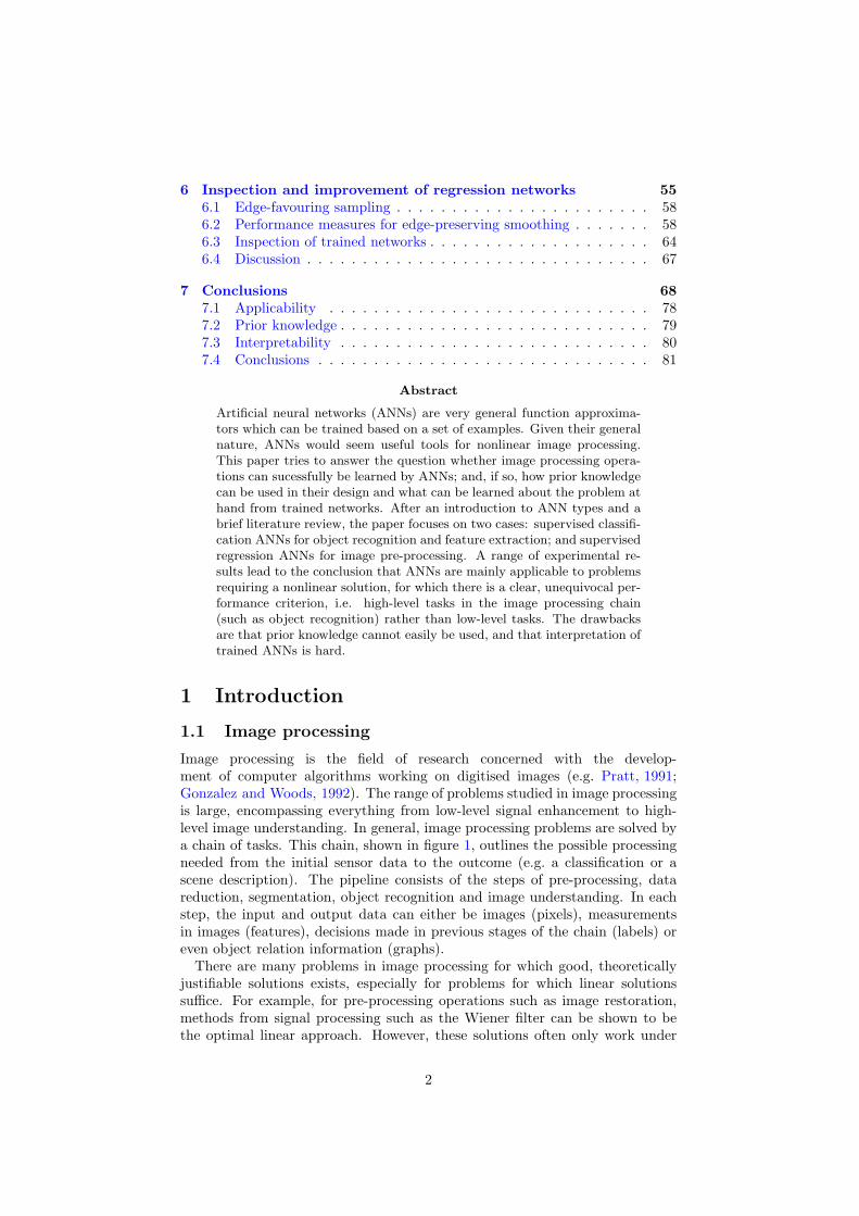
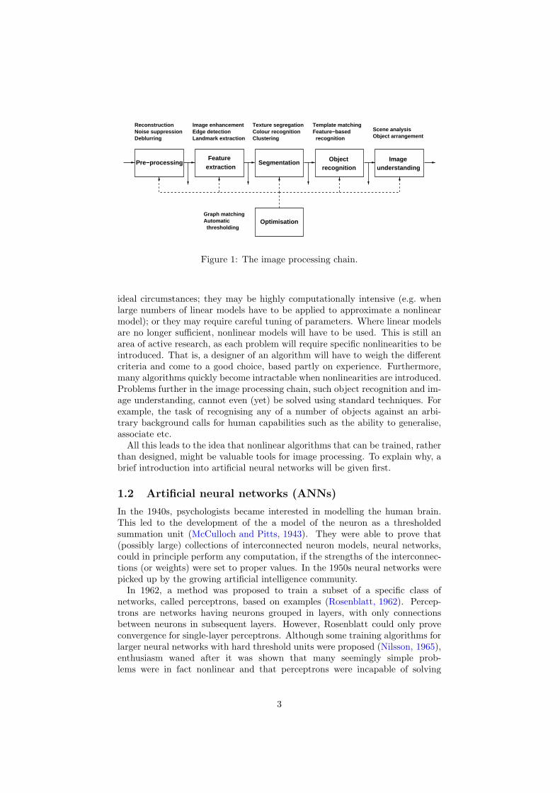
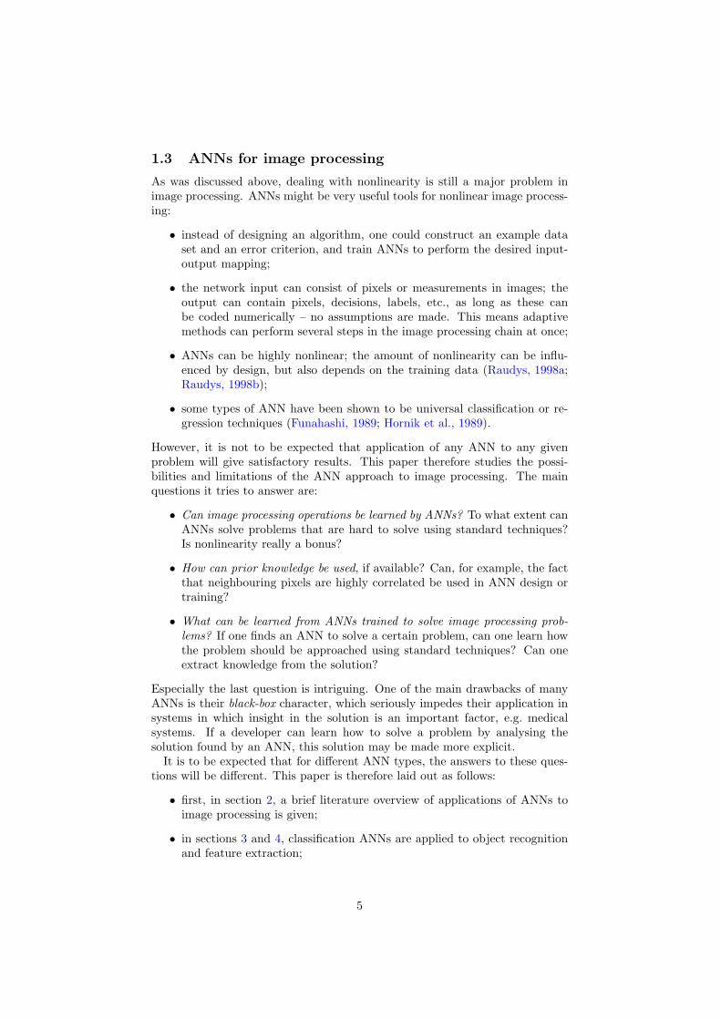
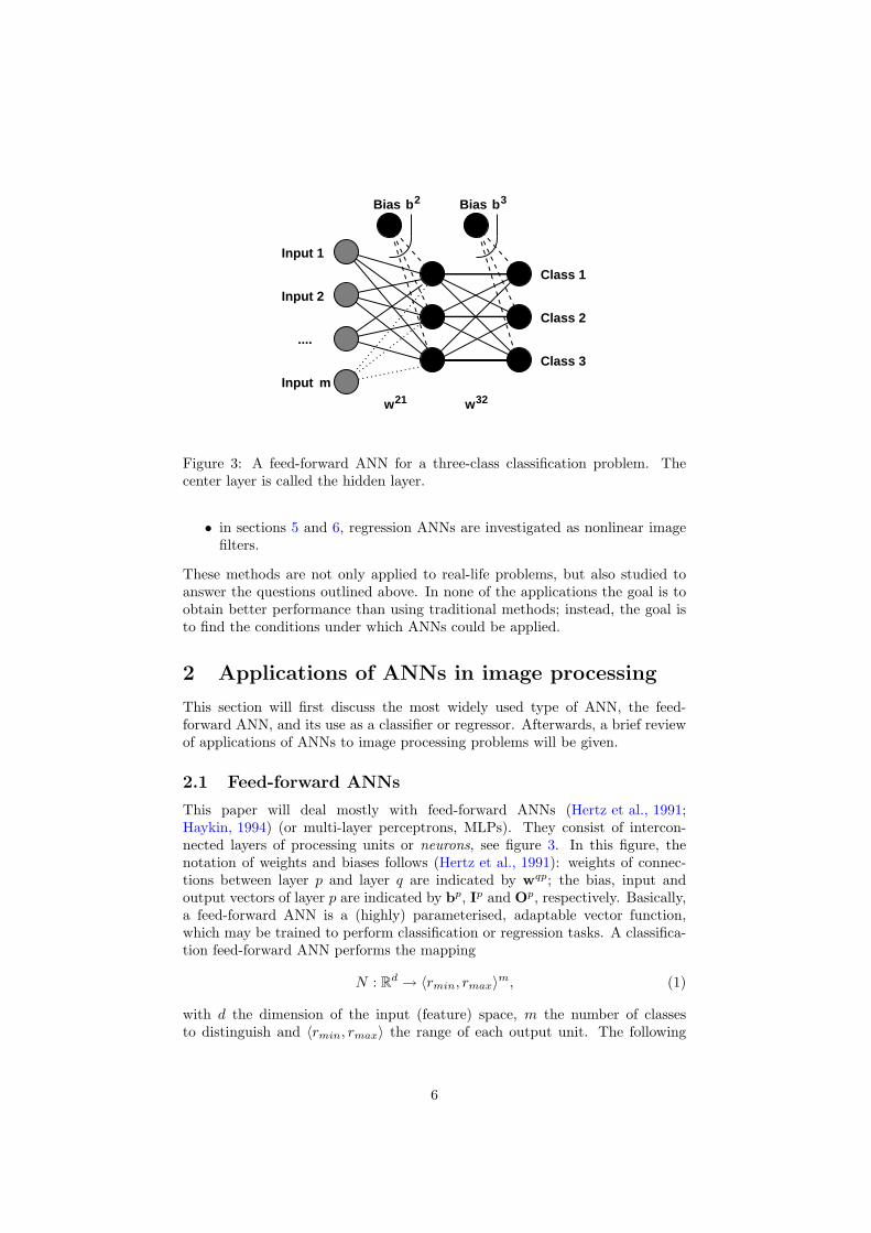
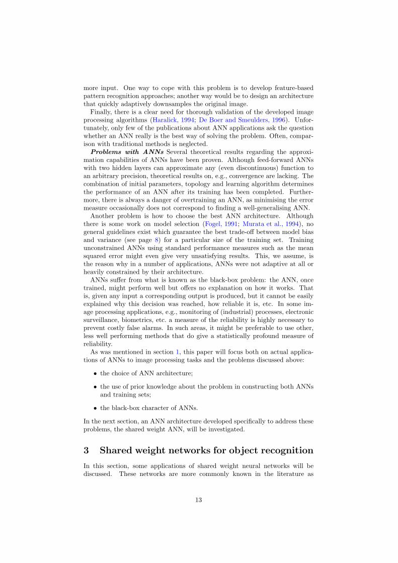
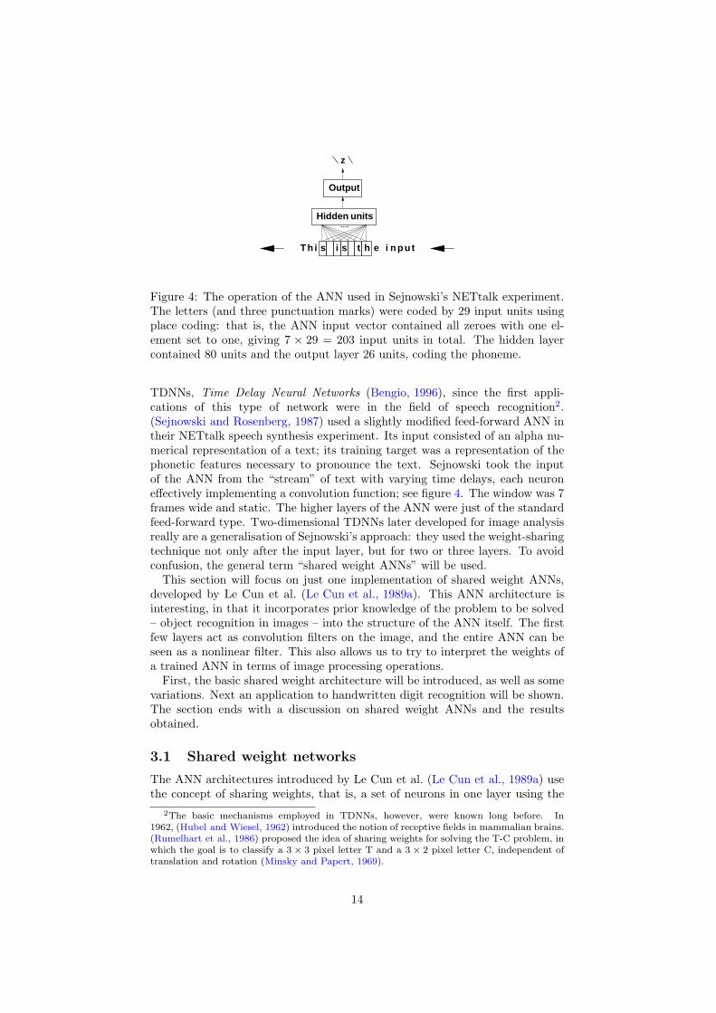
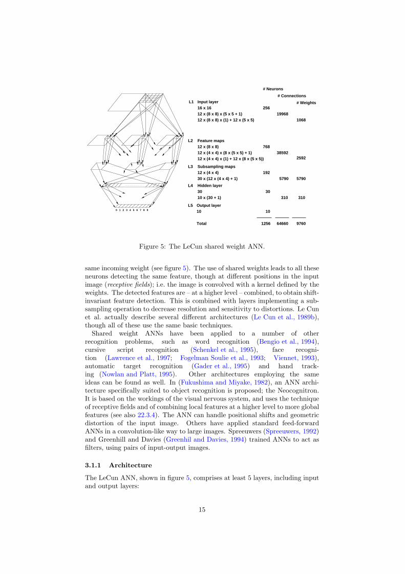
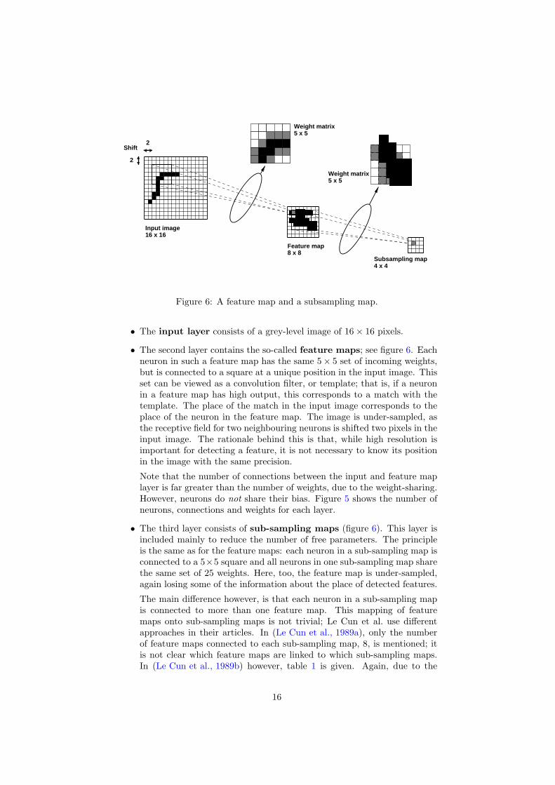
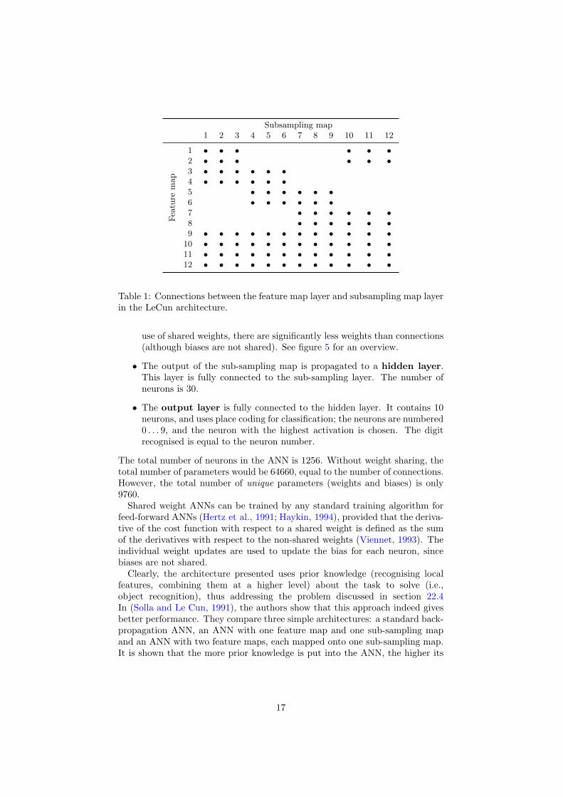
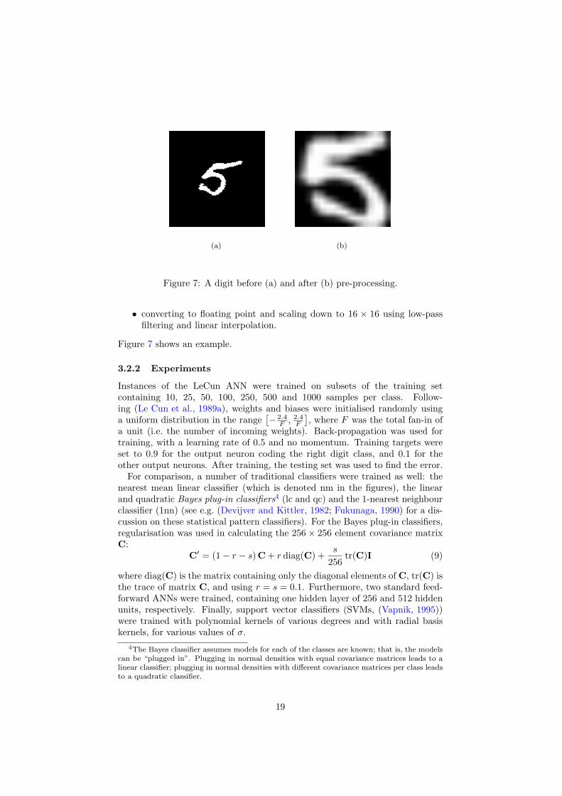
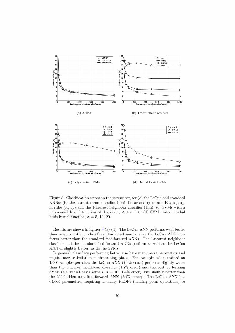
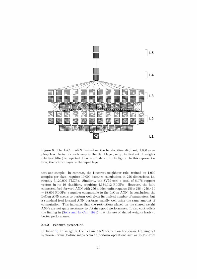
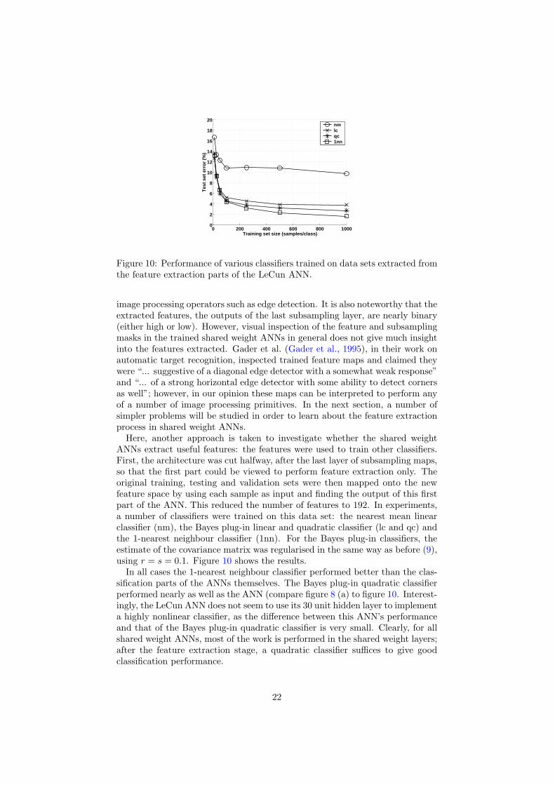
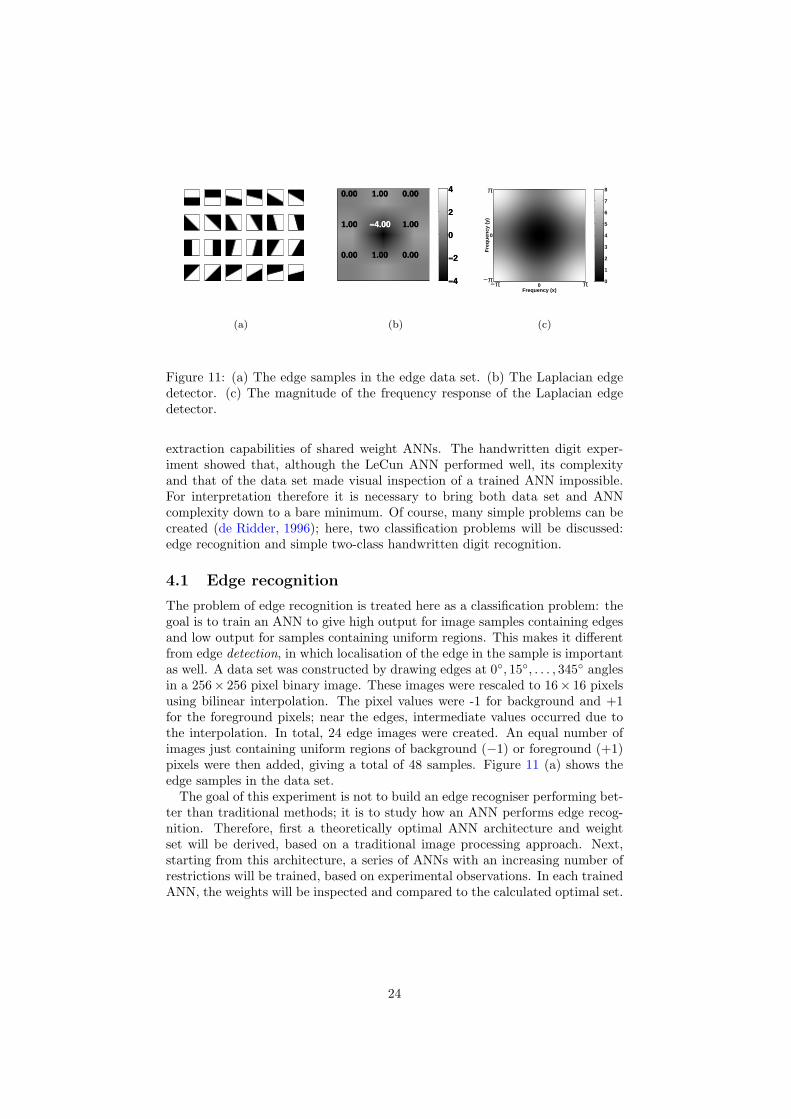
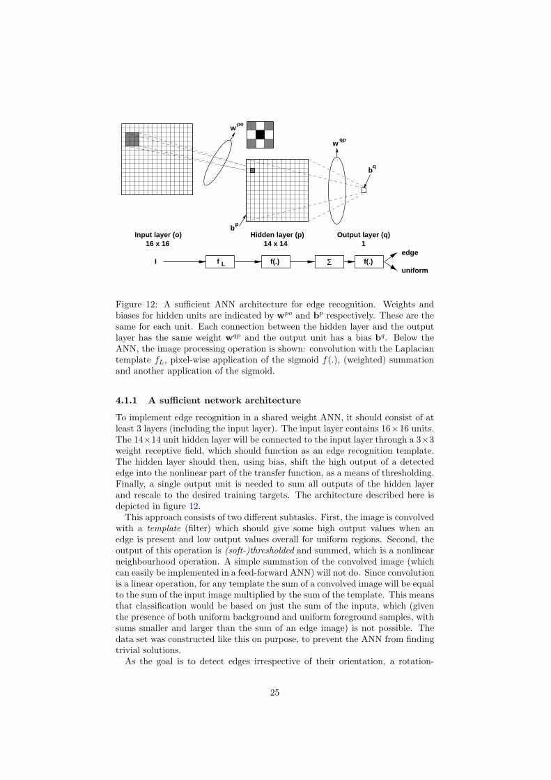
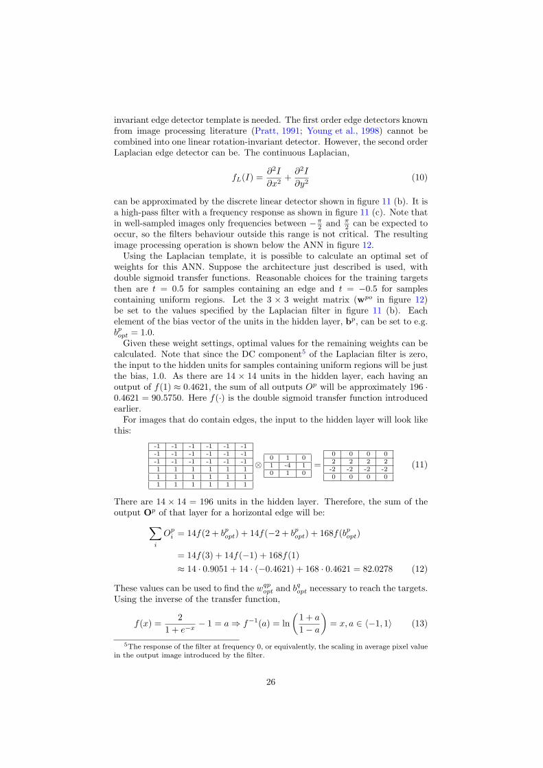
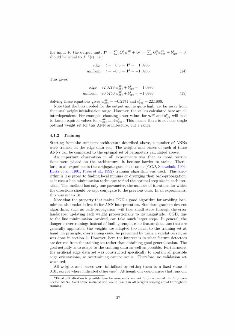
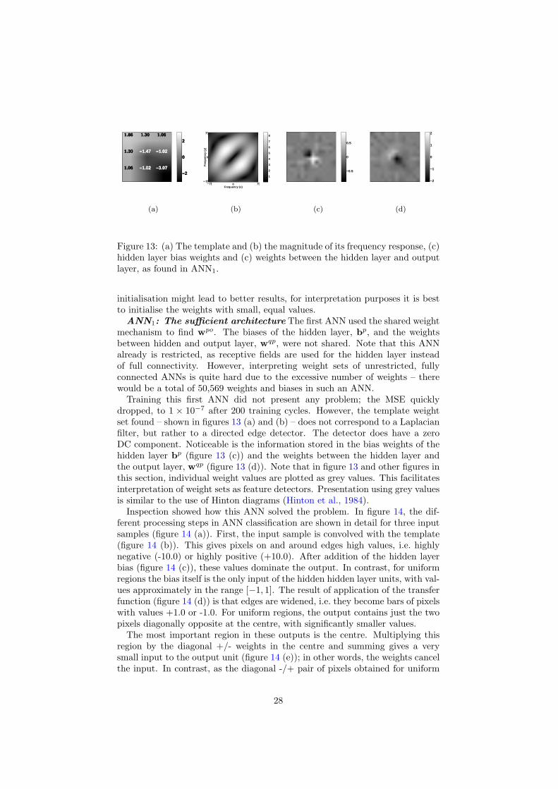
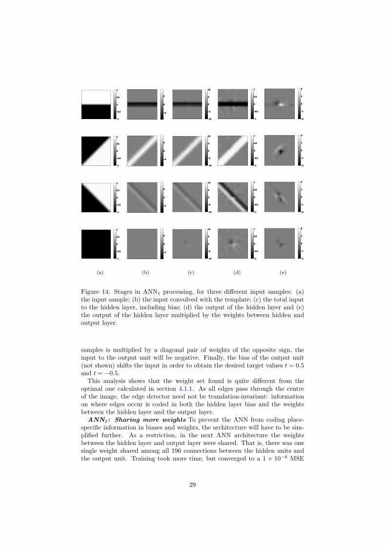
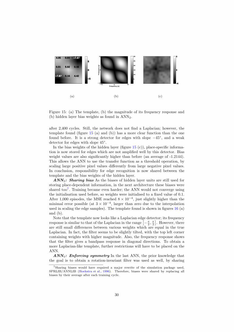
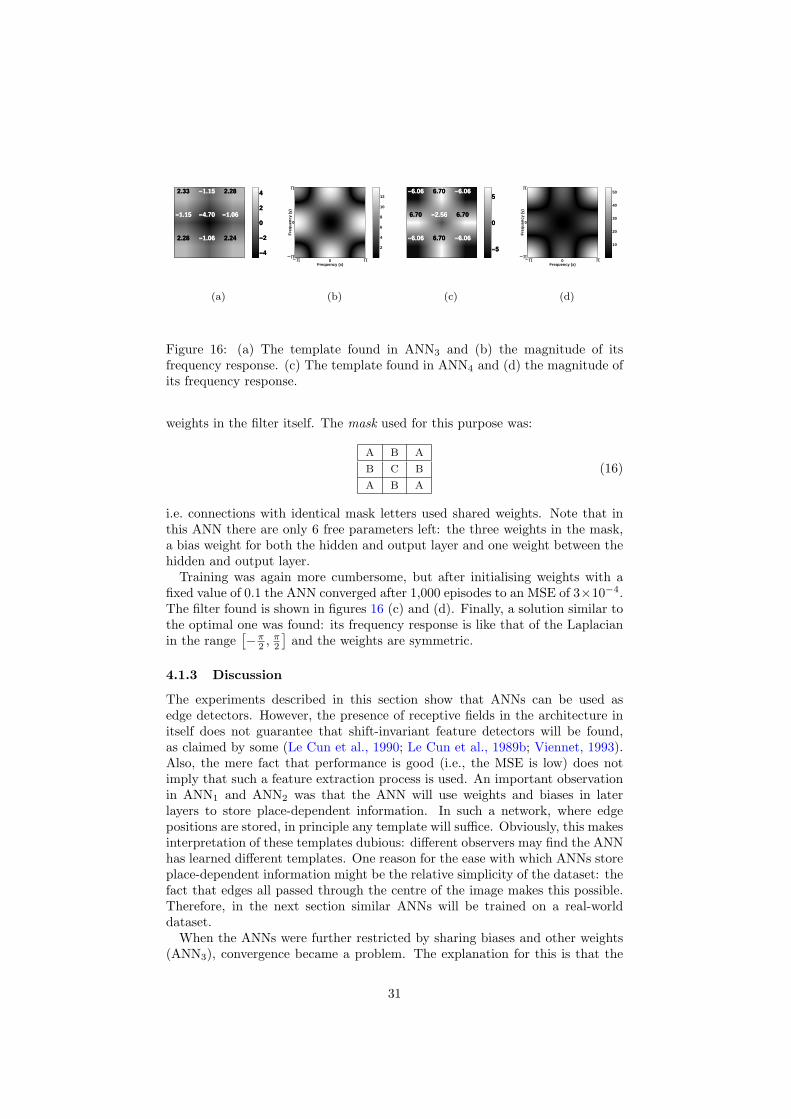
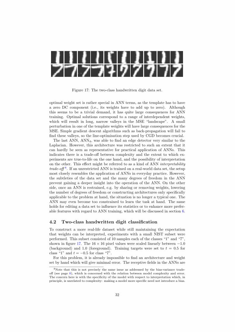
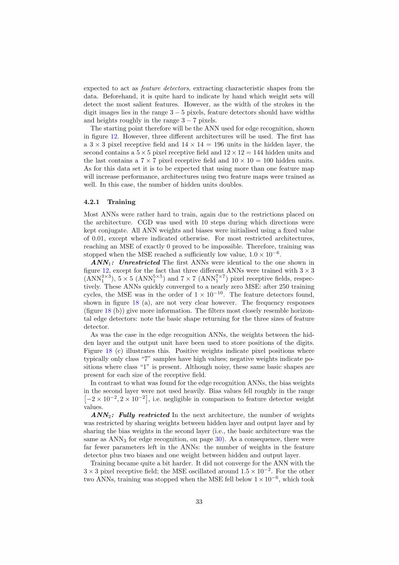
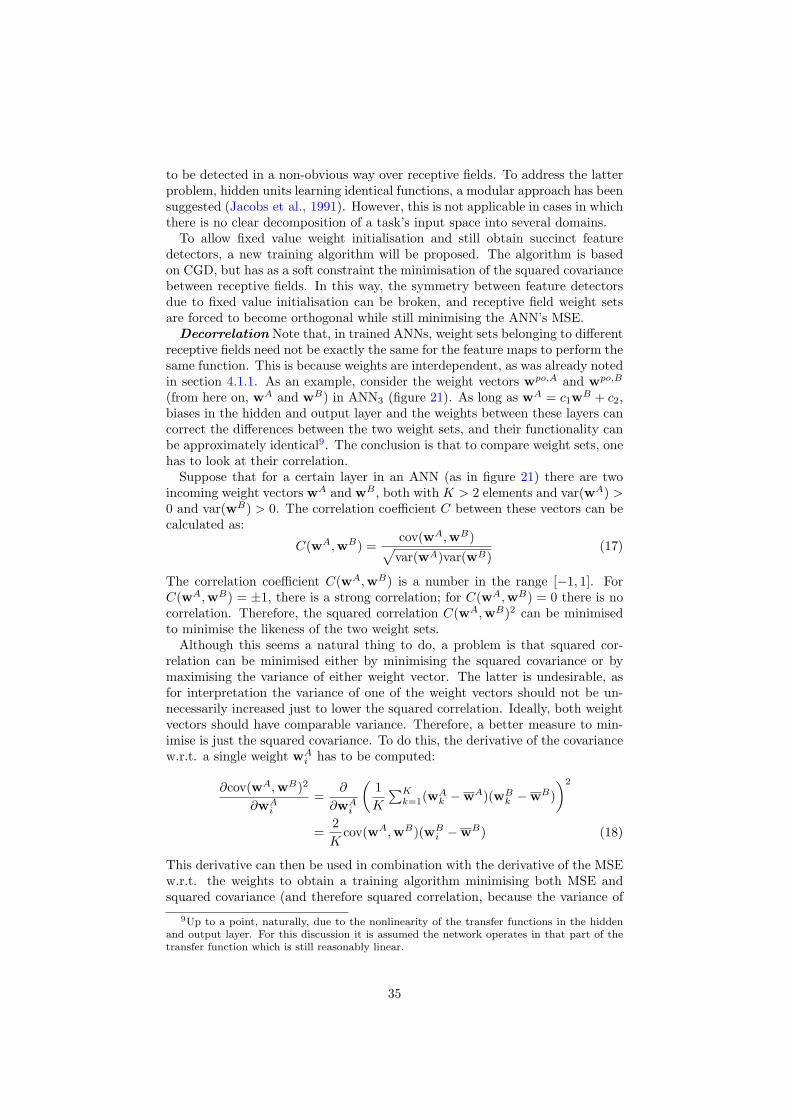
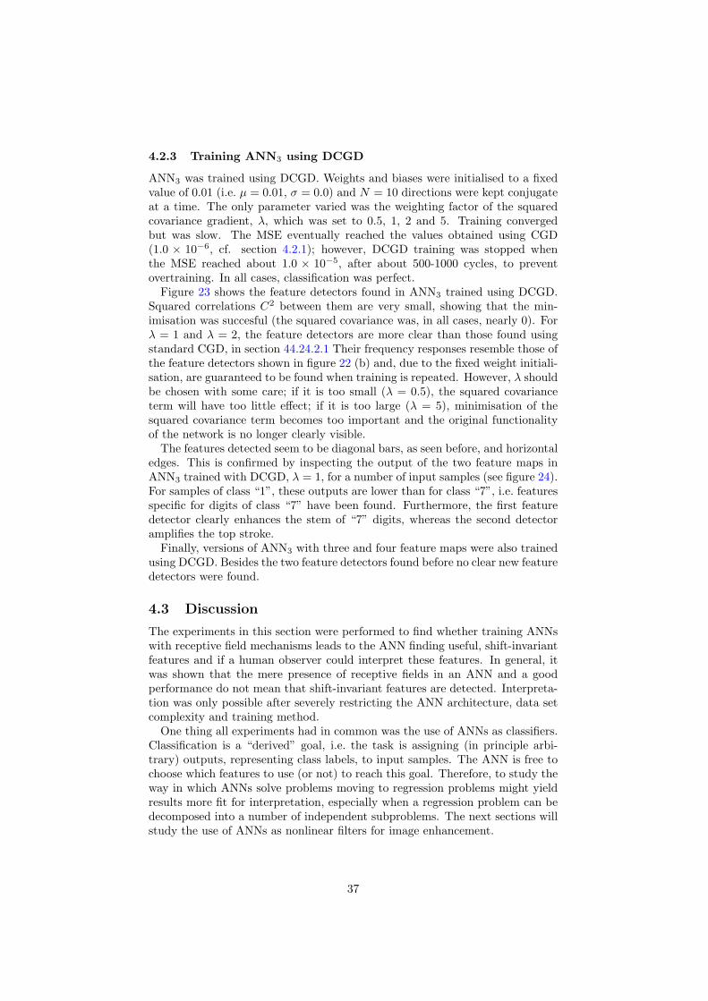
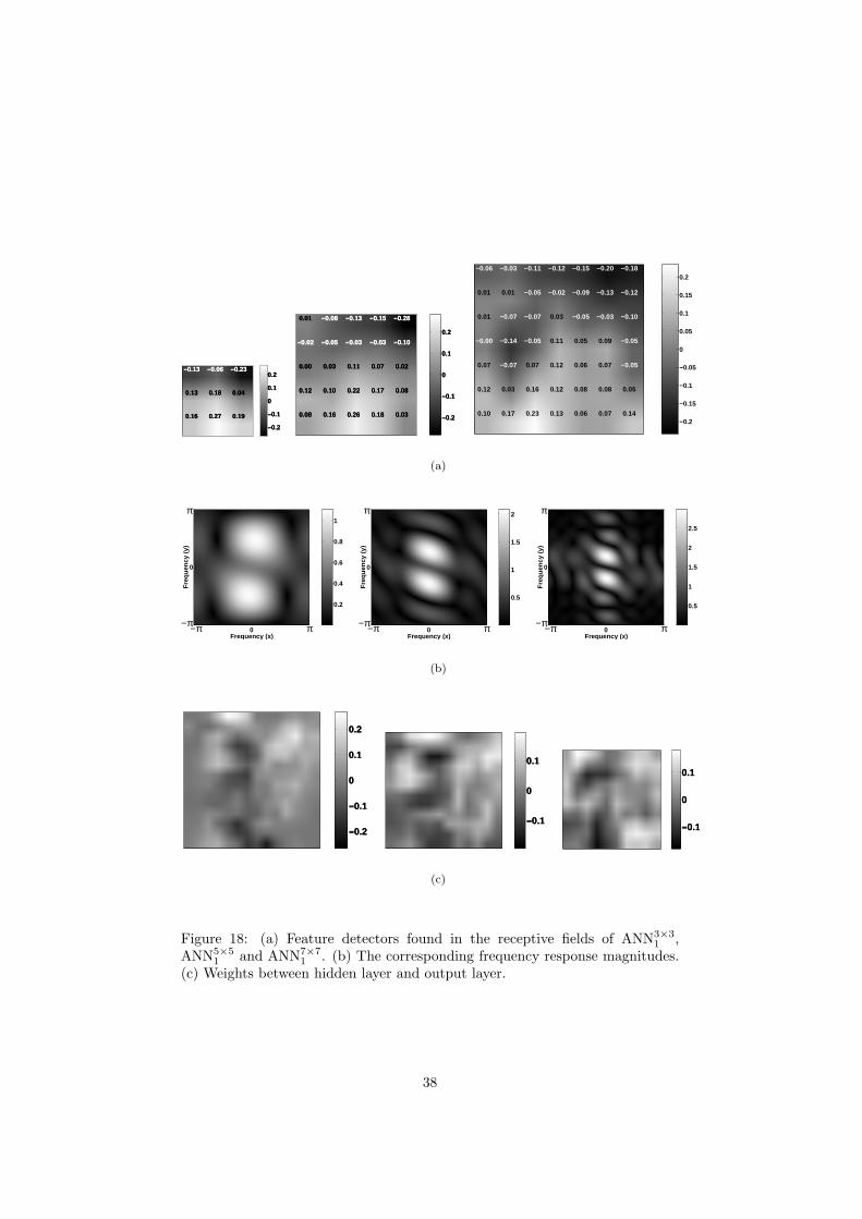
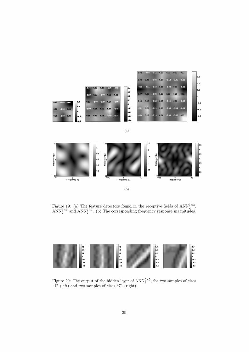
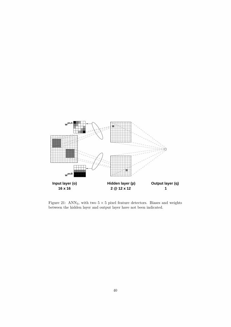
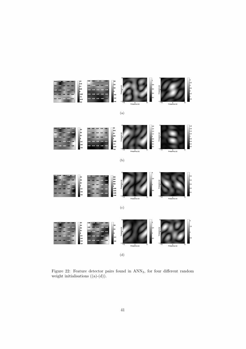
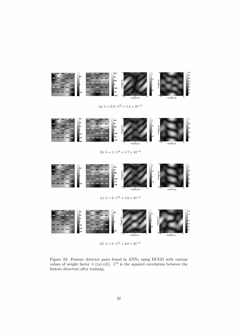
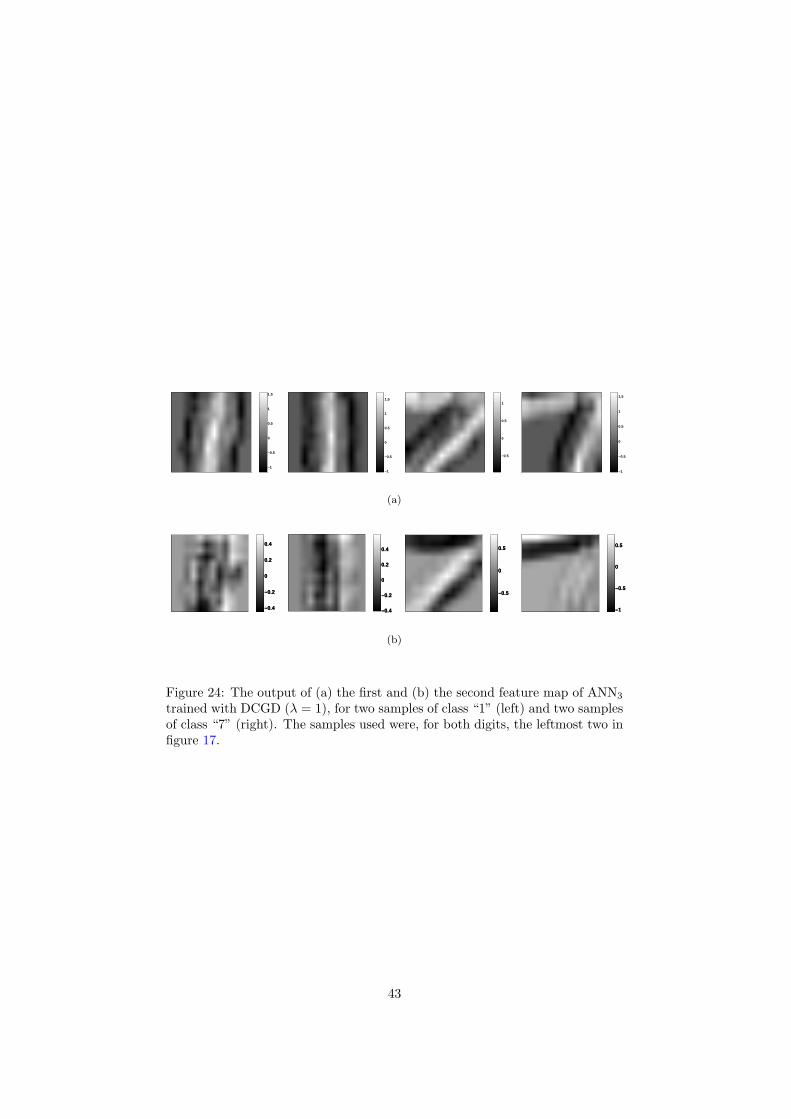
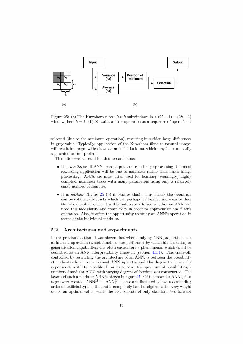
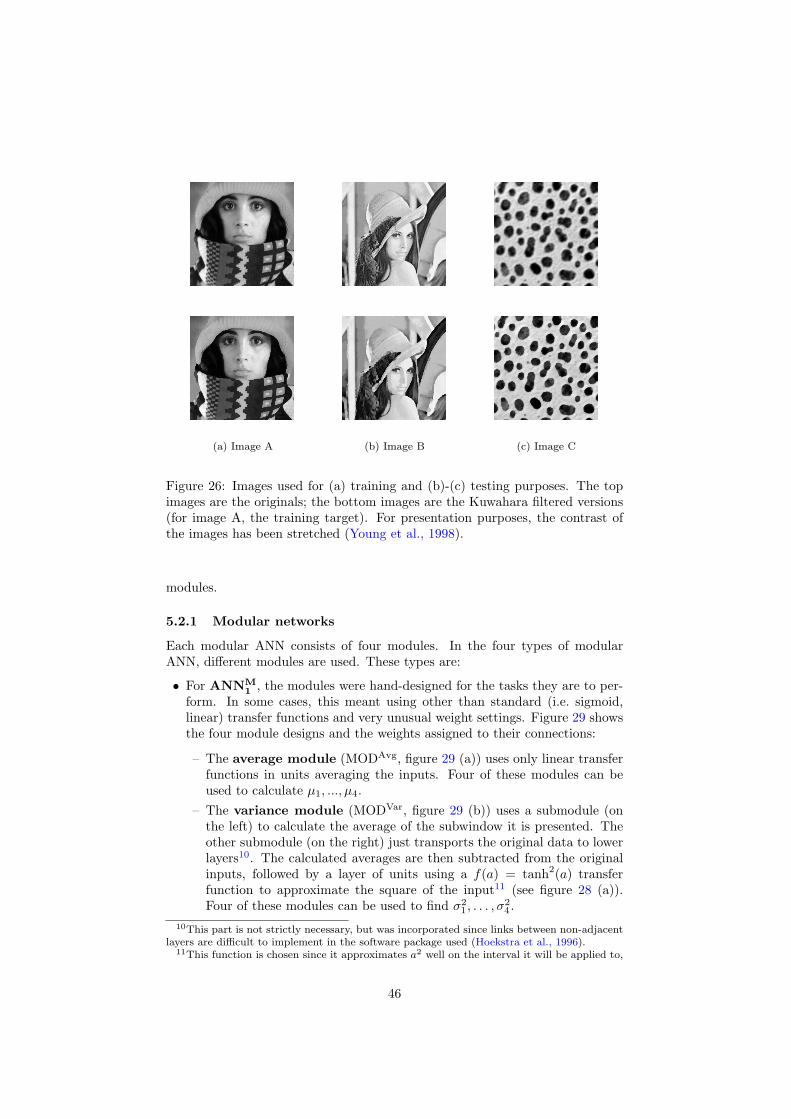
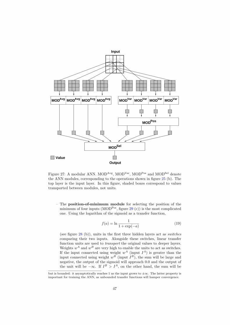
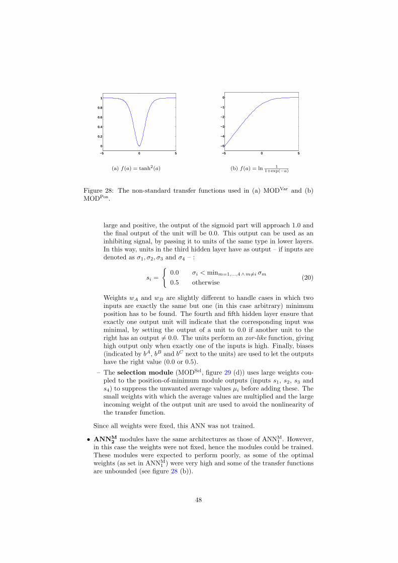
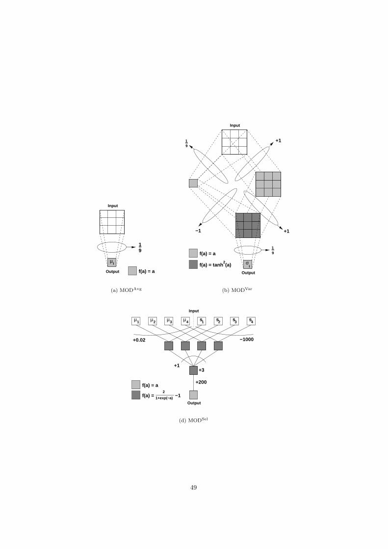
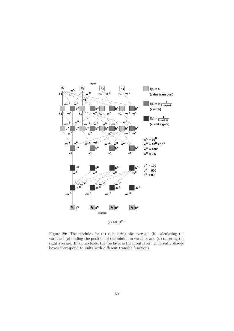
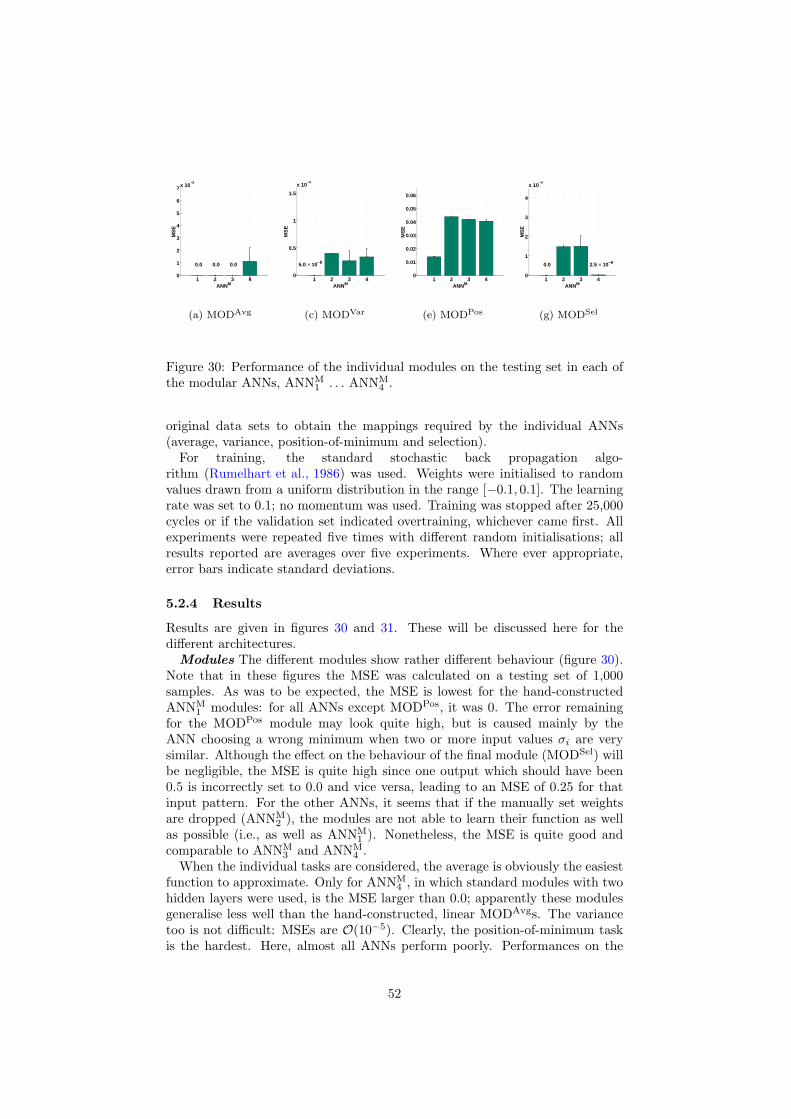
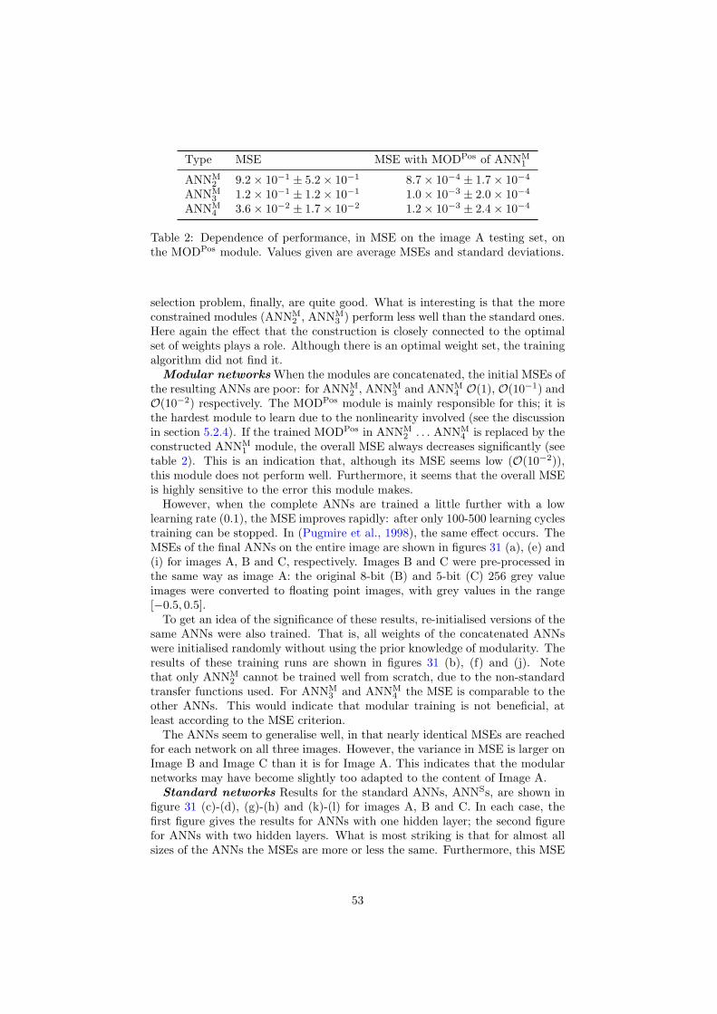
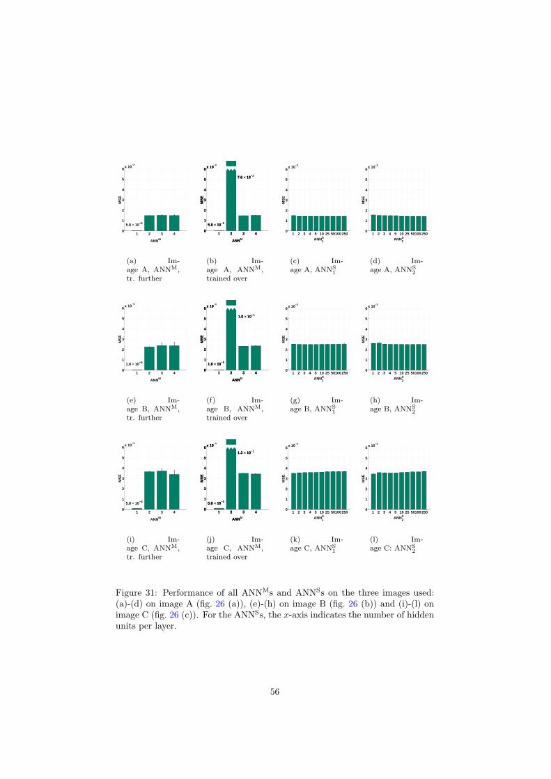
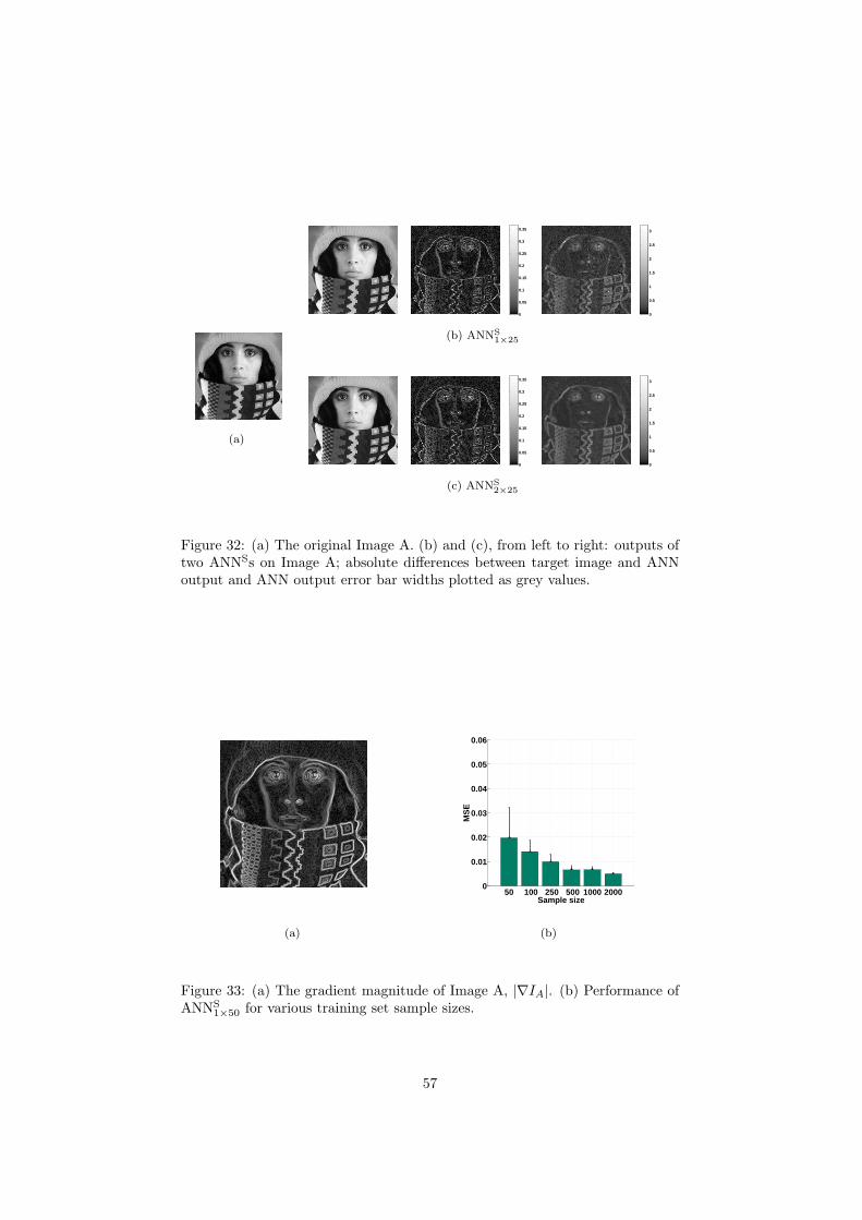
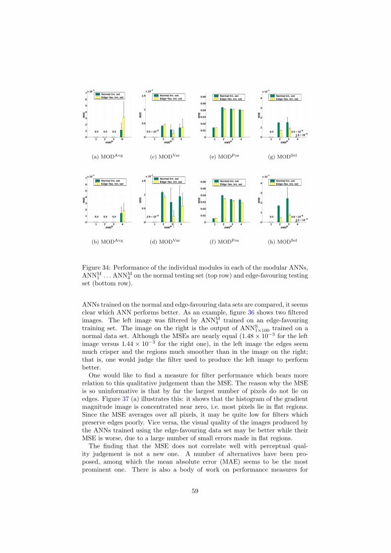
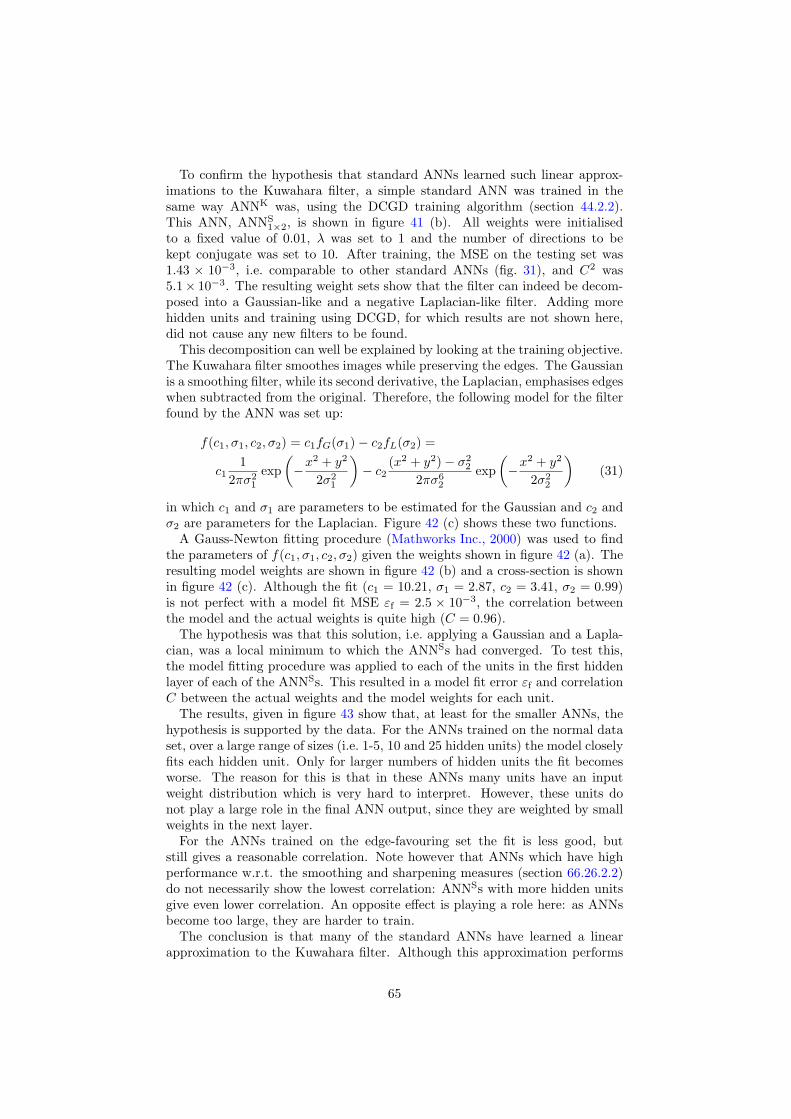
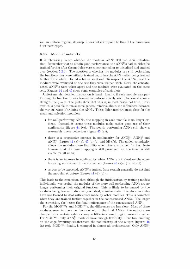
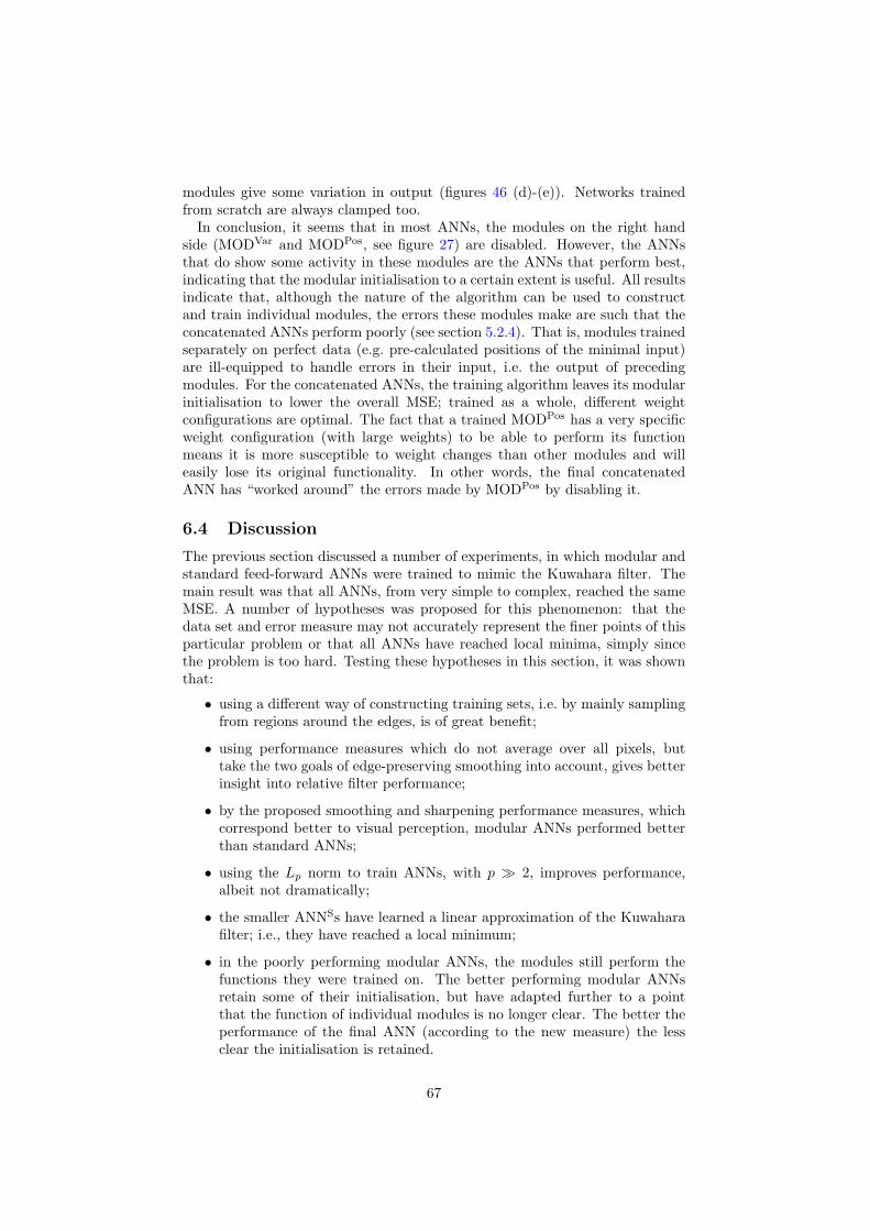
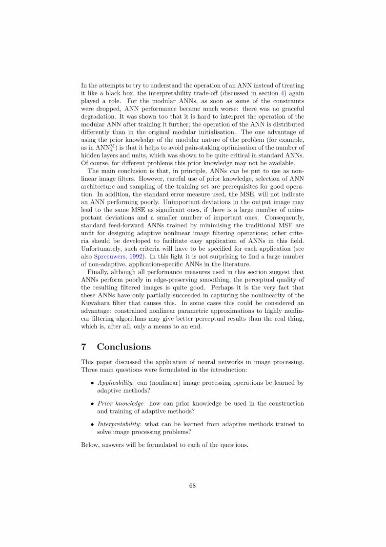
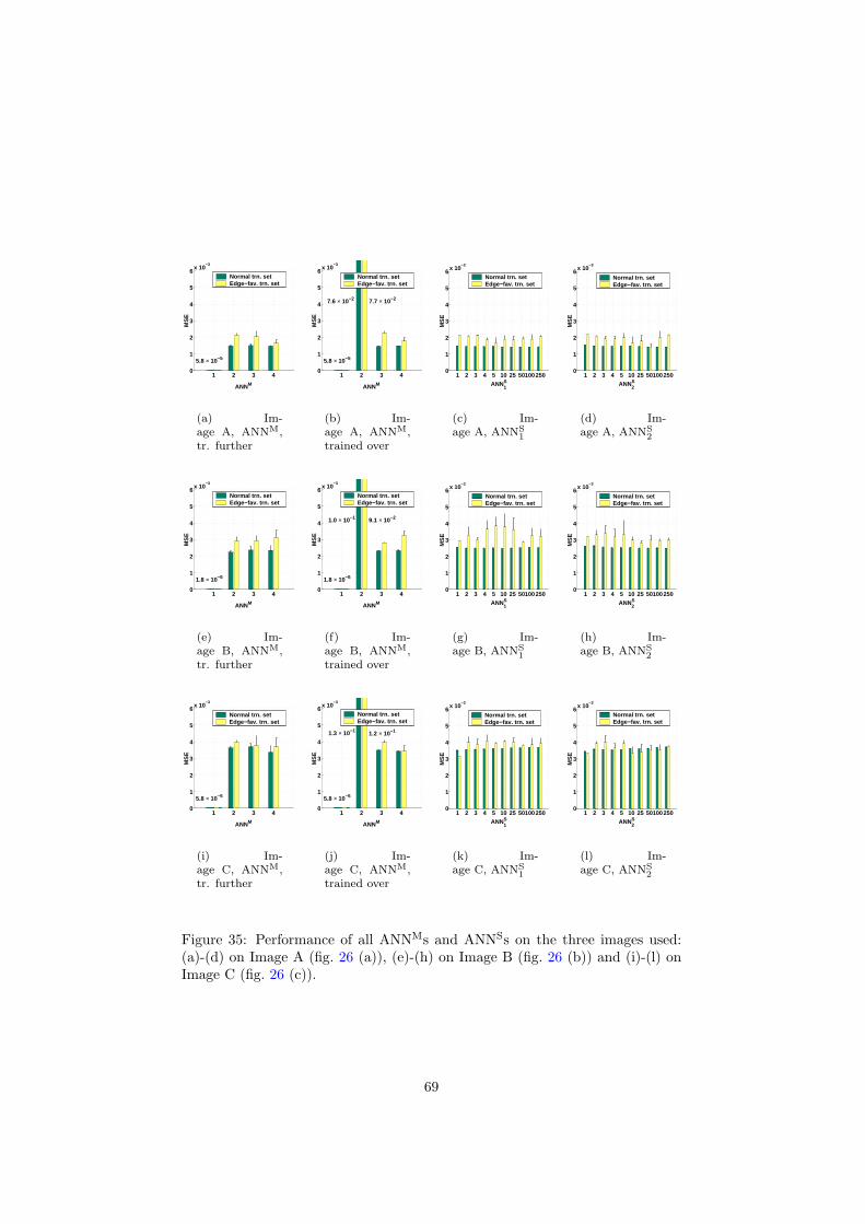
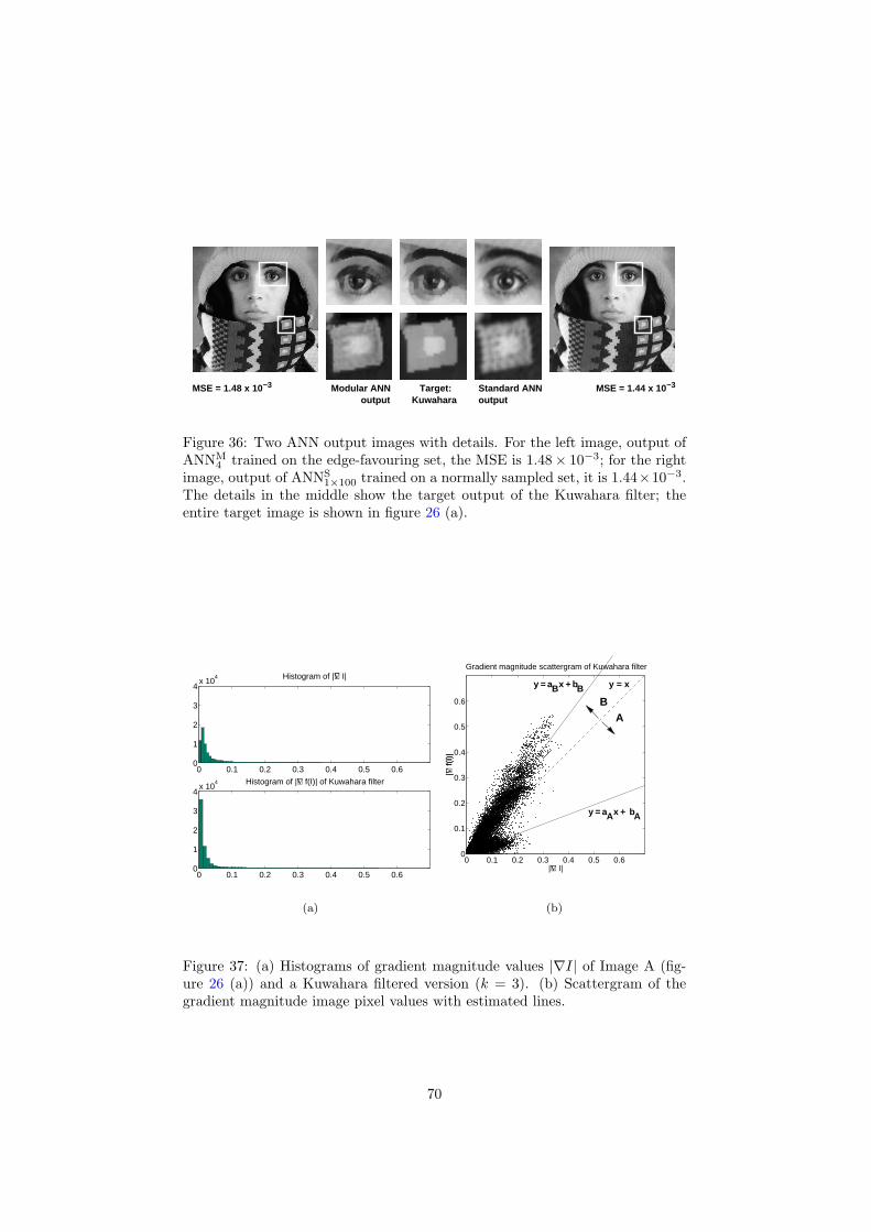
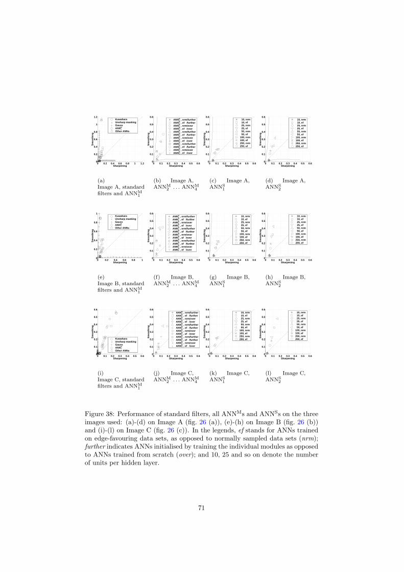
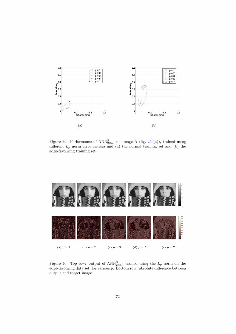
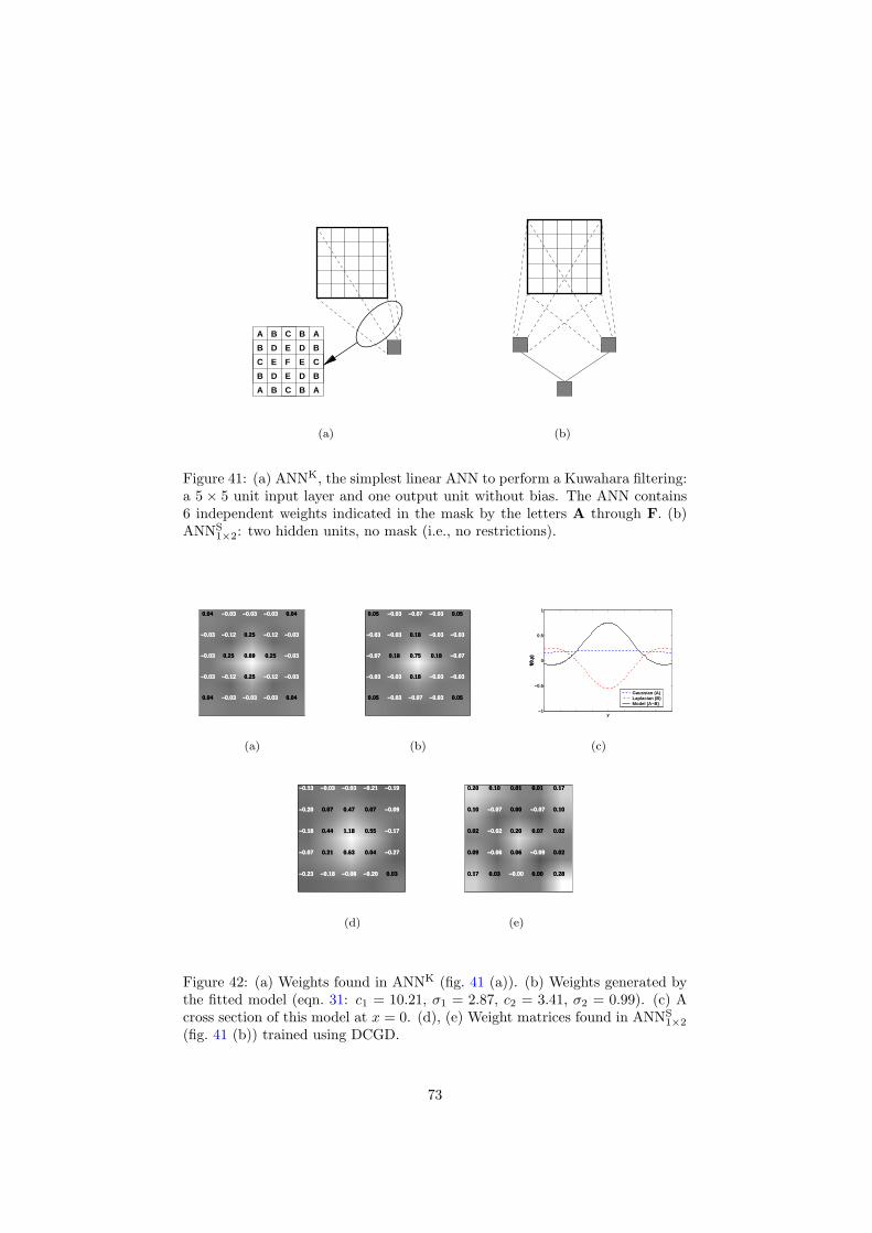
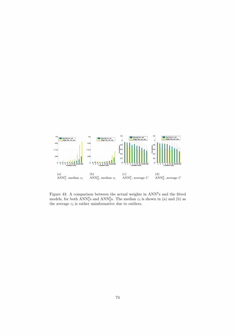
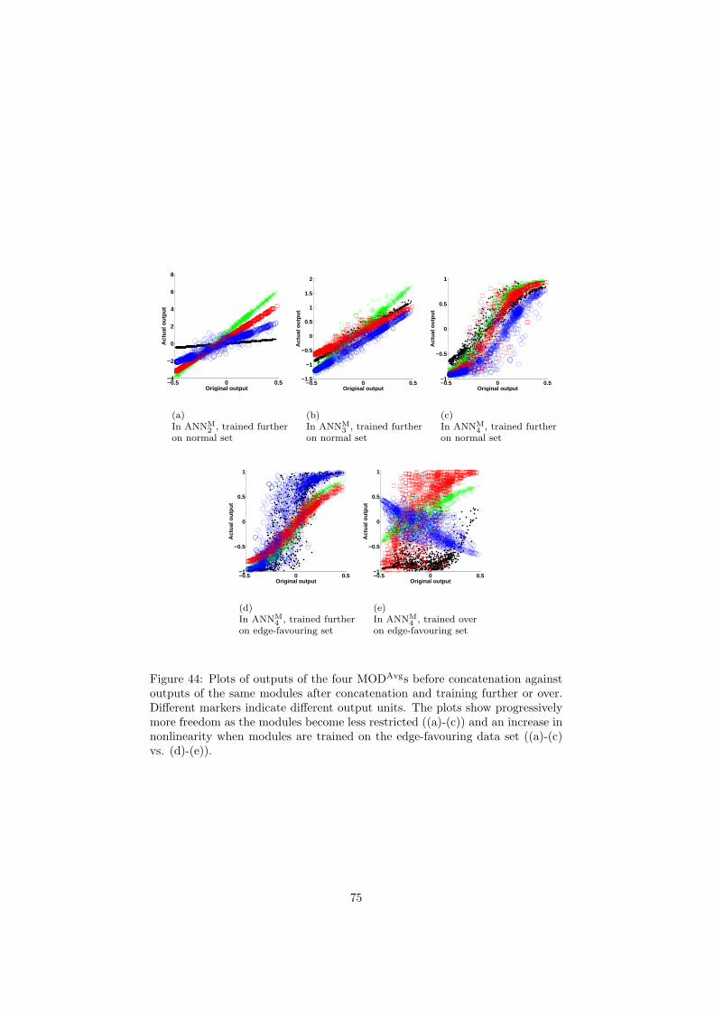
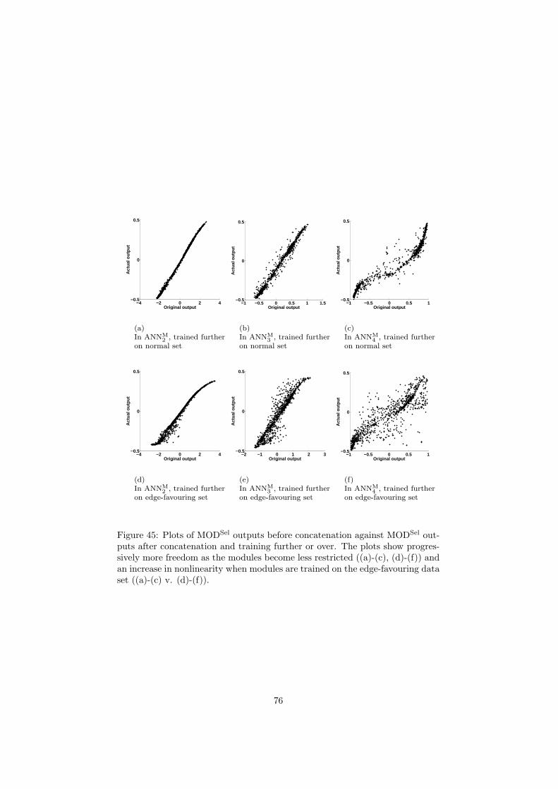
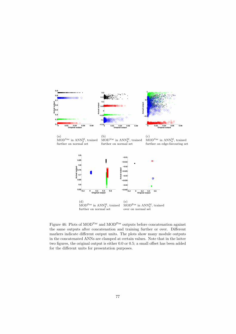


![Comparing nonlinear regression analysis and …Construc &ii Comparing nonlinear regression analysis and artificial neural networks [...]• M. A. Benbouras et al. 277 been mentioned](https://img.pdfslide.net/doc/110x75/5e62d9b36867275f530dc625/comparing-nonlinear-regression-analysis-and-construc-ii-comparing-nonlinear.jpg)