NONLINEAR MODEL PREDICTIVE CONTROL SCHEMES WITH GUARANTEED STABILITY

H. CHEN* Institut fUr Systemdynamik und Regelungstechnik Universitiit Stuttgart, 70550 Stuttgart, Germany email: chen@isr.uni-stuttgart.de

F. ALLGOWER Institut fur Automatik, Eidg. Techn. Hochschule Zurich CH-8092 Zurich, Switzerland email: allgower@aut.ee.ethz.ch

1 An introduction to nonlinear model predictive control

Model predictive control (MPC), also referred to as moving horizon control or reced­ing horizon control, has become an attractive feedback strategy, especially for linear or nonlinear systems subject to input and state constraints. In general, linear and nonlinear MPC are distinguished. Linear MPC refers to a family of MPC schemes in which linear models are used to predict the system dynamics, even though the dynamics of the closed-loop system is nonlinear due to the presence of constraints. Linear MPC approaches have found successful applications, especially in the pro­cess industries (Richalet, 1993). A complete overview on industrial MPC techniques with details and comparisons is given by Qin and Badgwell (1996), where more than 2200 applications in a very wide range from chemicals to aerospace industries are also summarized. By now, linear MPC theory is quite mature. Important issues such as stability are well addressed (see for example (Lee, 1996) for an overview).

Systems in the process industry are, however, in general inherently nonlinear, although linear models are widely used to solve control problems. In addition, higher product quality specifications and increasing productivity demands, tighter environmental regulations and demanding economical· considerations in the process industry require systems to be increasingly complex and to be operated closer to the boundary of the admissible operating region. In these cases, linear models are

·currently with: Department of Electronic Engineering, Jilin University of Technology, 130025 Changchun, PR China. Email: chenh@jut.edu.cn

465

R. Berber and C. Kravaris (eds.), Nonlinear Model Based Process Control, 465-494. © 1998 Kluwer Academic Publishers.

466

obviously not adequate to describe the process dynamics and nonlinear models have to be used.

In this paper, we want to review some of the available nonlinear MPC schemes with an emphasis on stability and robustness issues. We mainly concentrate on the continuous time case, but sometimes state the discrete version if this simplifies the exposition.

1.1 Principle and properties

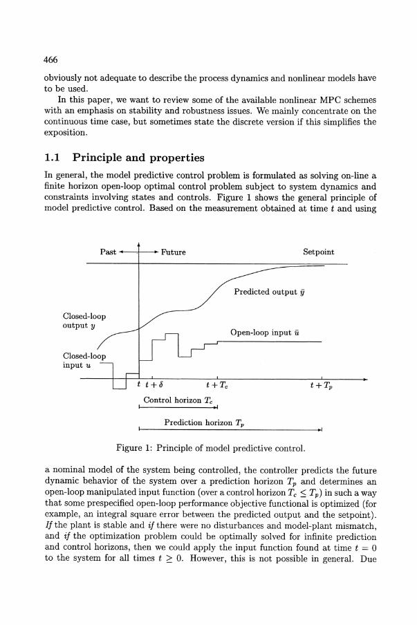
In general, the model predictive control problem is formulated as solving on-line a finite horizon open-loop optimal control problem subject to system dynamics and constraints involving states and controls. Figure 1 shows the general principle of model predictive control. Based on the measurement obtained at time t and using

Past ---,If-- Future Setpoint

Closed-loop output y

t t + 0 t+Tc

Control horizon Tc .1

Predicted output fj

Open-loop input u

Prediction horizon Tp

Figure 1: Principle of model predictive control.

t+Tp

a nominal model of the system being controlled, the controller predicts the future dynamic behavior of the system over a prediction horizon Tp and determines an open-loop manipulated input function (over a control horizon Tc :S Tp) in such a way that some prespecified open-loop performance objective functional is optimized (for example, an integral square error between the predicted output and the setpoint). If the plant is stable and if there were no disturbances and model-plant mismatch, and if the optimization problem could be optimally solved for infinite prediction and control horizons, then we could apply the input function found at time t = 0 to the system for all times t ~ O. However, this is not possible in general. Due

467

to disturbances and/or model-plant mismatch, the true system behavior is different from the predicted behavior. In order to incorperate some feedback mechanism into the scheme, the open-loop manipulated input function found will be implemented only until the next measurement becomes available. We assume that this will be the case every 8 time-units, where 8 denotes the "sampling time". Updated with the new measurement, at time t+ 8, the whole procedure - prediction and optimization - is repeated to find a new input function, with the control and prediction horizons moving forward, (for this reason, MPC is also referred to as moving horizon control or receding horizon control). That results in a discrete feedback control with an implicit control law, because dosed-loop inputs are calculated by solving on-line the optimization problem at each sampling time. Thus, MPC is characterized by the following features:

• Prediction: In contrast to other feedback controllers that calculate the con­trol action based on the present or past state (or output) information, model predictive controllers determine the control action based on the predicted fu­ture dynamics of the syste,m being controlled. The model used to complete the prediction can be linear or nonlinear, time-continuous or discrete, determinis­tic or stochastic, etc. Because the future response of the system is predicted, early control action can be taken so as to track, for example, a given reference trajectory with minimal tracking error.

• Optilllization: An objective functional that mathematically specifies the desired control performance is minimized on-line at each sampling instance. A commonly used objective functional is an integral weighted square error between predicted controlled variables and their desired references.

• Discrete lllanipulated inputs: Manipulated inputs are presented in a finite horizon and discrete manner, because, in general, the involved optimization problem can only be solved with numerical methods, especially when nonlinear systems and/or constraints are considered. A time-continuous input param­eterization and/or infinite prediction and control horizons lead to an infinite dimensional optimization problem that is numerically extremely demanding and often unsolvable. In order to get around that, the optimization problem is formulated with finite horizons and the inputs are discretized according to the sampling time and in the simplest case kept constant during the period between the sampling instances, as depicted in Figure 1.

• Constraints: In practice, most systems have to satisfy constraints on inputs and states. For example, an actuator reaches saturation and some states such as temperature and pressure are not allowed to exceed their limitations for the reason of safe operation, or some variables have to be held under certain threshold values to meet environmental regulations. Constraints automat­ically impose limitations on the achievable control performance, even if the system to be controlled is linear (Mayne, 1995). In extreme cases, the presence of constraints can destroy dosed-loop stability, if they are not considered when

468

a controller is designed (Chen, 1997). Even for cases where the constrained closed-loop systems are stable, the moqel predictive controller delivers bet­ter control performance, since it is able to take the current control action to minimize the errors caused by constraints that are predicted to become active in the future (Eaton and Rawlings, 1992). Thus, the feature of prediction provides in some sense an "active" handling of constraints, compared to other "passive" methods (e.g. (Gilbert and Tan, 1991; Mayne and Schroeder, 1994)) .

• Multivariable systems: Multivariable controllers are often required to im­prove control performance. In the framework of MPC, multiple inputs and multiple outputs can be straightforwardly handled by using multivariable models for the prediction.

1.2 Model predictive control vs. optimal control

Theoretically, an optimal feedback control law can be found as a solution of the corresponding Hamilton-Jacobi-Bellman partial differential equation (Bryson and Ho, 1969). However, in practice, solving the Hamilton-Jacobi-Bellman partial dif­ferential equation is very difficult, if not impossible, unless linear systems, quadratic objective functionals and no constraints are considered. In MPC, instead of solv­ing the Hamilton-Jacobi-Bellman partial differential equation, an open-loop optimal control problem is solved on-line repeatedly, initialized at the actual state. This is a considerably simpler task (Mayne, 1995), despite of the still expensive on-line com­putational demand. Especially for nonlinear systems subject to constraints, finite horizon nonlinear MPC provides a feasible approach to do optimal control in some sense.

1.3 State space models vs. I/O models

The history of MPC began with an attempt to use the powerful computer technol­ogy to improve the control of chemical processes that are constrained, multi variable and uncertain. In the late 70's and early 80's, Richalet and coworkers (Richalet et al., 1976; Richalet et al., 1978) developed Model Predictive Heuristic Control (MPHC) that is also referred to as Model Algorithmic Control (MAC) (Rouhani and Mehra, 1982), and Cutler and Ramaker (1980) developed Dynamic Matrix Con­trol (DMC). Due to their obvious advantages and successful applications, MPC has attracted more and more researchers from both the industrial and academic sides. Many formulations of the MPC problem have been proposed and implemented such as Linear Dynamic Matrix Control (Morshedi et al., 1985) (LDMC), Quadratic Dy­namic Matrix Control (QDMC) (Garda and Morshedi, 1986), Receding Horizon Tracking Control (RHTC) (Kwon and Byun, 1989), Generalized Predictive Con­trol (GPC) (Clarke et al., 1987a; Clarke et al., 1987b), Internal Model Control (IMC) (Garda and Morari, 1982; Garda and Morari, 1985a), Extended Horizon Adaptive Control (EHAC) (Y dstie, 1984), Extended Prediction Self-Adaptive Con­trol (EPSAC) (De Keyser and Van Cauwenberghe, 1985). Some of these methods

469

have different origins and different motivation. For example, GPC was meant as an extension to certain self-tuning control and adaptive control methods. For more complete surveys and comparisons between various MPC approaches we refer for example to (De Keyser et al., 1988; Garcia et al., 1989; Lee, 1996; Qin and Badg­well, 1996).

The main difference between the early versions of MPC lies in the type of models used to predict the future dynamics of the system being controlled. Impulse response models are used in MPHC, DMC is based on step response models, while GPC includes ARIMAX (Auto-Regressive Integrated Moving-Average with eXogenous input) models as are standard in the theory of prediction of stochastic processes.

Convolution models (impulse or step response models), where only input-output behavior is considered, are used in almost all early versions of MPC, for the reason that they can be easily obtained from process tests and signal processing techniques without significant fundamental modeling effort, even for very complex processes. However, convolution models are in general nonminimal representations and merely suitable to describe strictly stable systems. A convolution model with an integrator is able to approximately model an unstable system (Eaton and Rawlings, 1992; Hovd et al., 1993; Lee et al., 1994), however, the structure error in the model imposes a limitation on the achievable control performance. In addition, it is difficult to extend linear MPC approaches with convolution models to nonlinear systems. Using the special case of second-order Volterra models, Genceli and Nikolaou (1995), Doyle III and coworkers (Doyle III et al., 1995; Maner et al., 1994) have extended the DMC scheme in that respect. However, in order to represent nonlinear systems with a certain accuracy, much higher order Volterra models are required, whose coefficients may not be easy to identify any more. Another shortcoming of using convolution models is that a theoretical analysis of the closed-loop properties such as stability is difficult.

The interpretation of MPC in the state space setting, presented for example by Morari and Lee (1991) and Ricker (1991), provides a unified framework to un­derstand and generalize the existing MPC techniques, and more importantly, to systematically investigate the properties of the closed-loop system in the context of optimal control. In addition, state space model based MPC approaches can in principle be straightforwardly extended to nonlinear systems, just using nonlinear state space models.

1.4 Finite horizon predictive control

Consider a class of systems being described by the following general nonlinear set of ordinary differential equations

x(t) = f (x(t), u(t)), x(O) = xo

subject to input and state constraints

u(t) E U, 'Vt ~ 0

x(t) E X, 'Vt ~ 0,

(1)

(2a)

(2b)

470

where x(t) E IRn and u(t) E IRm denote the vectors of states and manipulated inputs, respectively. In the simplest form, U and X are specified as follows:

U := {u E IRmlumin :s U :s u max } X := {x E IRnlxmin :s x :s xmax} ,

where Umin, Umax , Xmin and Xmax are given constant vectors.

(3a)

(3b)

In order to distinguish clearly between the system and the system model used to predict the future "within" the controller, we denote the internal variables in the controller by a bar (for example X, u) to indicate that the predicted values need not and will not be the same as the actual values. This is also true for the undisturbed case with no model-plant mismatch, if only a finite horizon is used. Instead of the continuous time t a discrete time k will be used for discrete systems, i.e., k, x(k), u(k) and so on will be used.

1.4.1 Controller set~p

Usually, the finite horizon open-loop optimal control problem described in Sec­tion 1.1 is mathematically formulated as follows:

Problem 1 Find

with

subject to

min J (x(t), u(·), Te, Tp) u(·)

x = I(x, u), x(t) = x(t)

u(r) E U, r E [t,t+Te]

u(r) = u(t + Te), r E [t + Te , t +Tp]

x(r) EX, r E [t, t + Tp],

where Tp and Te are prediction and control horizons with Te :s Tp.

(4)

(5)

(6a)

(6b)

(6c)

(6d)

The function F specifies the desired control performance that can arise for example from economical and ecological considerations. The standard quadratic form is the simplest and most used one:

(7)

where Xs and Us denote given reference trajectories, that can be constant or time­varying; Q and R denote positive definite, symmetric weighting matrices. More commonly, with output equation y = g(x), function F can be for example chosen as

F(y, u) = (y - Ysf Q(y - yJ + (u - usf R(u - us), (8)

471

where y s are the given output references. In order for (xs, us) to be feasible, the point (xs, us) should be contained in the

interior of X x U. For the stabilization problem, it can be assumed, without loss of generality, that (0,0) is the steady state point of interest of the system. Note the initial condition in (6a): The system model used to predict the future in the controller is initialized by the actual system states, that are in general assumed to be measured or must be estimated. Equation (6c) is not a constraint but implies that beyond the control horizon the predicted control takes a constant value equal to that at the last step of the control horizon. For a numerical implementation, the input function is in general parameterized in a step-shaped manner. As shown in Figure 1, u(·) on [t, t+Tcl satisfies u(r) = canst for r E [t+ j8, t+ (j + 1)8),j = 0,1,'" ,Ne, where Ne = .'If and 8 denotes the sampling period.

An optimal solution to the optimization problem (existence assumed) is denoted by u*(·; x(t), Te, Tp) : [t, t +Te] --+ U. According to the principle of MPC, the open­loop optimal control problem will be solved repeatedly, when new measurements are available at the sampling instances t = j8, j = 0,1,' ". The optimal closed-loop control is defined by

u*(r) := u*(·; x(t), Tel Tp) , r E [t, t + 8]. (9)

Model-plant mismatch and disturbances are generally not represented in the optimization problem. At most, they are indirectly considered in that their effect is assumed to be constant over the prediction horizon. For example, an additional unknown but constant state vector d(t) E IRq that is used to represent disturbances and uncertainties is introduced into the system description:

x = f(x,u,d)

d= O.

1.4.2 Advantages and drawbacks

(1Oa) (1Ob)

Since Problem 1 is formulated in a finite horizon manner and, the input function can be finitely parameterized, a numerical solution is then possible in principle. Moreover, the F function in the cost functional can be chosen arbitrarily to meet any economical and ecological requirements. Trajectory (output) tracking problem can also be taken into account in this framework. However, because a finite horizon criterion is not designed to deliver an asymptotic property such as stability (Bitmead et al., 1990), a general finite horizon MPC scheme cannot guarantee closed-loop stability. Closed-loop stability can only be achieved by a suitable tuning of design parameters such as prediction horizon, control horizon and weighting matrices. This makes an independent specification of the desired control performance difficult. In addition, due to the presence of nonlinearities, a system behaves differently for different operating conditions and tuning for stability often cannot deliver satisfying results for various operating conditions. Thus, guaranteed stability, i.e., stability independent of the choice of performance parameters, is of great interest not only in theory but also for practitioners.

472

In the following, we discuss nonlinear model predictive control schemes that deliver guaranteed stability.

2 Nominal stability of nonlinear MPC schemes

An intuitive way to achieve guaranteed stability is to use an infinite horizon cost functional (Bitmead et al., 1990), that results in general in an infinite dimensional (or, approximated appropriately, a very high dimensional) optimization problem. For nonlinear systems, solving such an optimization problem is very difficult, if not impossible. For linear systems, using an additional terminal term in the cost functional the infinite horizon optimization problem can be transformed into a finite horizon one (Rawlings and Muske, 1993; Scokaert and Rawlings, 1996). In this approach, the prediction is exactly considered over an infinite horizon, but the input function to be determined on-line is only of finite horizon. This way, closed-loop stability can be guaranteed and the optimization problem is numerically solvable. In analogy to the linear case, nonlinear MPC schemes are developed, in which the open-loop optimal control problem is formulated in a finite horizon manner, but the prediction is considered over the infinite horizon in order to achieve closed-loop stability. Besides input and state constraints, so-called stability constraints (Mayne, 1995) have to be included into the finite horizon open-loop optimal control problem.

2.1 Predictive control with terminal equality constraints

The most widely suggested stability constraint is the terminal equality constraint (Keerthi and Gilbert, 1988; Kleinman, 1970; Mayne and Michalska, 1990)

x(t + Tp) = 0, (11)

that forces the state to be zero at the end of the finite horizon. In the context of LQ control, the terminal equality constraint is quite intuitive, since it is equiv­alent to the infinite initial condition of the backwards Riccati equation, whose solution constitutes a stabilizing state feedback controller for linear controllable systems (Kleinman, 1970). In fact, if the terminal equality constraint is feasible, i.e., the system at the end of the finite horizon is at the origin and the input there­after is set to be zero, then the unperturbed nominal system stays at the origin forever. This way, the prediction horizon can be thought of as expanding exactly to infin~ty.

For continuous systems, Mayne and Michalska (1990) show that under some rather strong assumptions, MPC with the terminal equality constraint (11) and a quadratic objective functional is able to stabilize a class of nonlinear constrained sys­tems. The strong assumptions are needed to ensure that the optimal value function is continuously differentiable and can serve as Lyapunov function for the closed-loop system. Those assumptions are relaxed in (Michalska and Mayne, 1991) to ensure merely local Lipschitz continuity of the optimal value function. Analogous results for discrete systems are proposed by Keerthi and Gilbert (1988) and improved by Rawlings et al. (1994), where the optimization problem is formulated as follows:

473

Problem 2 Find (12)

with Np

J(X(k),7fNp):= LF(x(k+j),u(k+j)) (13) j=O

subject to

x(k + j + 1) = f (x(k + j), u(k + j)) , x(k) = x(k) (14a)

u(k + j) E U, j E [0, Np] (14b)

x(k + Np ) = 0, (14c)

where Np = '!f and 7fNp = {u(k), u(k + 1),···, u(k + N p)}.

Under reasonable conditions, asymptotic stability for the discrete closed-loop system can be proven for both finite Np'and Np -+ 00 (Meadows et al., 1995).

Motivated by practical considerations, Genceli and Nikolaou (1995) derive an end condition for nonlinear S1S0 MPC with second-order Volterra models, where the system to be controlled is assumed to be stable. The optimization problem is formulated as follows:

Problem 3 Find

(15)

subject to

N

y(k + j) = d(k + j) + L giu(k + j - i) i=l

M M

+ L L gili2 u(k + j - idu(k + j - i 2 ), j E [1, Np ] (16a)

N

d(k + j) = d(k) = y(k) - L giu(k - i) i=l

M M - L L gili2 u(k - idu(k - i 2 ), j E [1, Np] (16b)

/lumin ::; /luCk + j) ::; /lumax , j E [0, N e] (16c)

/luCk + Ne + j) = 0, j E [Ne + 1, Np ] (16d)

Umin ::; u(k + j) ::; Umax , u(k + j) = u(k + j - 1) + /luCk + j), j E [0, Ne](16e) d(k) + Gu(k + N e ) + GU(k + N e )2 = ys (16f)

474

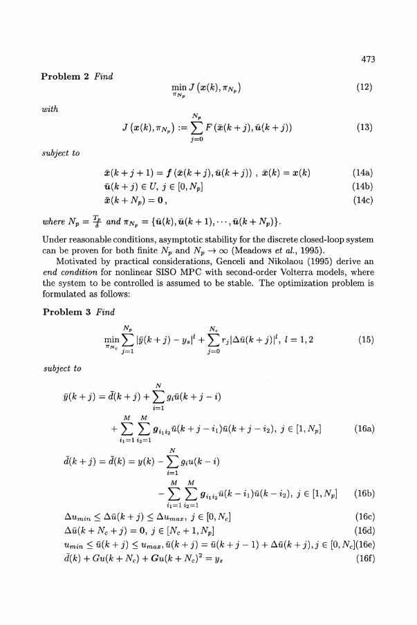
In this formulation, gi and gi1 i2 are the coefficients of the second-oder Volterra model; Nand M represent the memory length of the Volterra series; Au denotes the increment ofthe controlinput U, i.e., Au(k) = u(k)-u(k-1); rj,j = 0,1,"" Nc are control move suppressions. The additional constraint (16f) is referred to as end condition, where

M M

G = L L gi1 i2'

il=l i2=1

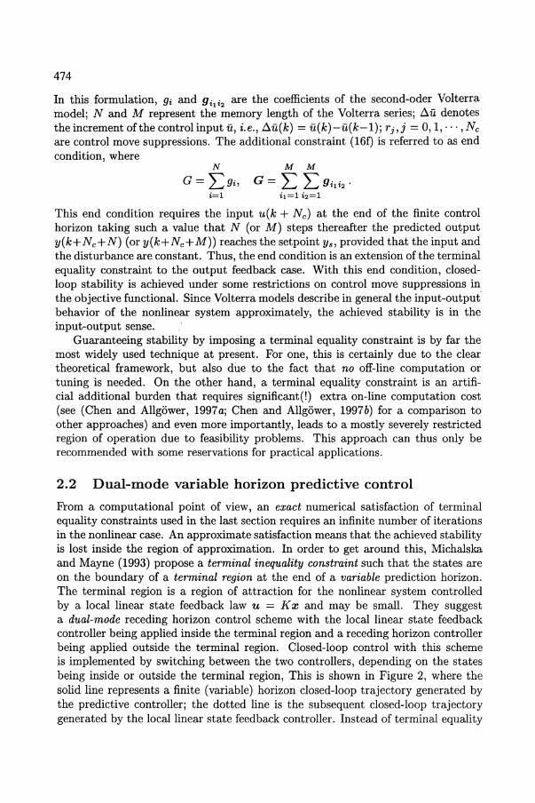
This end condition requires the input u(k + N c ) at the end of the finite control horizon taking such a value that N (or M) steps thereafter the predicted output y(k+Nc+N) (or y(k+Nc+M)) reaches the setpoint Ys, provided that the input and the disturbance are constant. Thus, the end condition is an extension of the terminal equality constraint to the output feedback case. With this end condition, closed­loop stability is achieved under some restrictions on control move suppressions in the objective functional. Since Volterra models describe in general the input-output behavior of the nonlinear system approximately, the achieved stability is in the input-output sense.

Guaranteeing stability by imposing a terminal equality constraint is by far the most widely used technique at present. For one, this is certainly due to the clear theoretical framework, but also due to the fact that no off-line computation or tuning is needed. On the other hand, a terminal equality constraint is an artifi­cial additional burden that requires significant(!) extra on-line computation cost (see (Chen and Allgower, 1997a; Chen and Allgower, 1997b) for a comparison to other approaches) and even more importantly, leads to a mostly severely restricted region of operation due to feasibility problems. This approach can thus only be recommended with some reservations for practical applications.

2.2 Dual-mode variable horizon predictive control

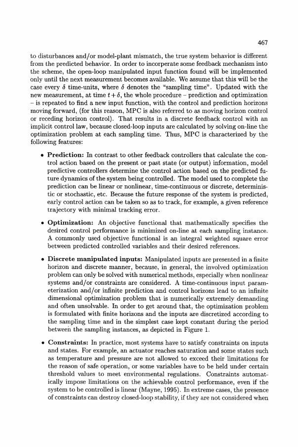
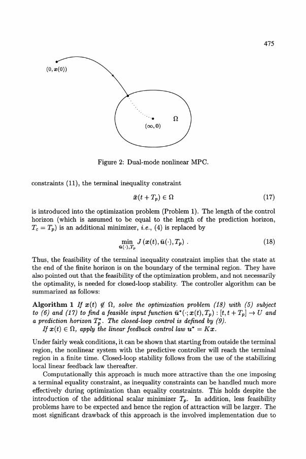
From a computational point of view, an exact numerical satisfaction of terminal equality constraints used in the last section requires an infinite number of iterations in the nonlinear case. An approximate satisfaction mean'S that the achieved stability is lost inside the region of approximation. In order to get around this, Michalska and Mayne (1993) propose a terminal inequality constraint such that the states are on the boundary of a terminal region at the end of a variable prediction horizon. The terminal region is a region of attraction for the nonlinear system controlled by a local linear state feedback law u = K x and may be small. They suggest a dual-mode receding horizon control scheme with the local linear state feedback controller being applied inside the terminal region and a receding horizon controller being applied outside the terminal region. Closed-loop control with this scheme is implemented by switching between the two controllers, depending on the states being inside or outside the terminal region, This is shown in Figure 2, where the solid line represents a finite (variable) horizon closed-loop trajectory generated by the predictive controller; the dotted line is the subsequent closed-loop trajectory generated by the local linear state feedback controller. Instead of terminal equality

475

(0, :1:(0))

. ". (00,0)

Figure 2: Dual-mode nonlinear MPC.

constraints (11), the terminal inequality constraint

(17)

is introduced into the optimization problem (Problem 1). The length of the control horizon (which is assumed to be equal to the length of the prediction horizon, Tc = Tp) is an additional minimizer, i.e., (4) is replaced by

min J (x(t), u(·), Tp) . u(.),Tp

(18)

Thus, the feasibility of the terminal inequality constraint implies that the state at the end of the finite horizon is on the boundary of the terminal region. They have also pointed out that the feasibility of the optimization problem, and not necessarily the optimality, is needed for closed-loop stability. The controller algorithm can be summarized as follows:

Algorithm 1 If x(t) f/. n, solve the optimization problem (18) with (5) subject to (6) and (17) to find a feasible input function u*(·; x(t), Tp) : [t, t + Tp] --+ U and a prediction horizon T;. The closed-loop control is defined by (9).

If x(t) En, apply the linear feedback control law u* = Kx.

Under fairly weak conditions, it can be shown that starting from outside the terminal region, the nonlinear system with the predictive controller will reach the terminal region in a finite time. Closed-loop stability follows from the use of the stabilizing local linear feedback law thereafter.

Computationally this approach is much more attractive than the one imposing a terminal equality constraint, as inequality constraints can be handled much more effectively during optimization than equality constraints. This holds despite the introduction of the additional scalar minimizer Tp. In addition, less feasibility problems have to be expected and hence the region of attraction will be larger. The most significant drawback of this approach is the involved implementation due to

476

the required switching between control strategies and the need to determine a local stabilizing state feedback gain K and the terminal region f2.

2.3 Contractive predictive control

Yang and Polak (1993) propose another way to achieve closed-loop stability of nonlinear MPC. They introduce a stability constraint imposing the state vector to contract by a prespecified factor. This constraint is referred to as contraction constraint. The optimization problem is then formulated as follows:

Problem 4 Find

subject to

min J (x(t), u(·), Te) u(·),Tc

x = f(x, 11.), x(t) = x(t)

11.(7) E U, 7 E [t,t+Tel

Te E [t+T1 ,t+T2l

X(7) EX, 7 E [t, t + Tel

Ilx(t + Te)112 :s a21Ix(t)112 max Ilx(7)112 :s ,821Ix(t)112 ,

TE[t,t+Tcl

(19)

(20a)

(20b)

(20c)

(20d)

(20e)

(20f)

where Tl is the least time needed to solve the optimization problem and T2 is an a priori upper limit on the control horizon.

The constraints (20e) and (20f) with 0: E (0,1) and ,8 E [1,00) are used to ensure closed-loop stability. Different from standard MPC, the entire input function over the interval [t, t + Tel found by solving the optimization problem (Problem 4) will be applied to the nonlinear system. Closed-loop exponential stability is proven by showing that Ilx(t + jTc)112 :s 0:2j llx(t)112 --+ 0 as j --+ 00 holds, when the existence of a solution to the optimization problem at the time ,t + jTc with j = 0,1,2" .. is assumed. However, this is a very strong assumption and cannot be guaranteed in general (Mayne, 1995). A complete algorithm and stability proof can be found in (De Oliveira and Morari, 1997).

The main advantage of this approach is its exponential stability property, be­cause of which asymptotic stability for observer based contractive predictive con­trollers can be established (see Section 4). However, this approach is not very attractive for applications, since the feasibility of the optimization problem at each sampling instance cannot be guaranteed. Choosing large 0: E (0,1) might obtain the required feasibility, but large a implies a slow contraction of the state vector. Moreover, despite the free specification of the desired control performance by the objective functional, the achieved control performance will be influenced directly by the choice of design parameters 0: and ,8.

477

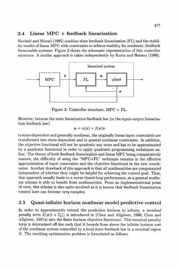
2.4 Linear MPC + feedback linearization Nevistic and Morari (1995) combine state feedback linearization (FL) and the stabil­ity results of linear MPC with constraints to achieve stability for nonlinear, feedback linearizable systems. Figure 3 shows the schematic representation of this controller structure. A similar approach is taken independently by Kurtz and Henson (1996).

r·--····························~~~~~:z·~·~···~;~~~:·· ............................... .

I-v--+--+i8~BI--+--'---.---'

MPC

, 1 L ............................ L .... -.... -.... -.... -.... -.... -.... -.... -..... -.... -.... -.... -.... -i ...... ~ ....................... :

Figure 3: Controller structure: MPC + FL.

However, because the state linearization feedback law (or the input-output lineariza­tion feedback law)

U = o:(x) + f3(x)v

is state-dependent and generally nonlinear, the originally linear input constraints are transformed into state-dependent and in general nonlinear constraints. In addition, the objective functional will not be quadratic any more and has to be approximated by a quadratic functional in order to apply quadratic programming techniques on­line. The theory of both feedback linearization and linear MPC being comparatively mature, the difficulty of using the "MPC+ FL" technique remains in the effective approximation of input constraints and the objective functional in the new coordi­nates. Another drawback of this approach is that all nonlinearities are compensated independent of whether they might be helpful for achieving the control goal. Thus, this approach usually leads to a worse closed-loop performance,.as a general nonlin­ear scheme is able to benefit from nonlinearities. From an implementational point of view, this scheme is also quite involved as it is known that feedback linearization control laws can become very complex.

2.5 Quasi-infinite horizon nonlinear model predictive control

In order to approximately extend the prediction horizon to infinity, a terminal penalty term E(x(t + Tp)) is introduced in (Chen and Allgower, 1996; Chen and Allgower, 1997 a) into the finite horizon objective functional. This terminal penalty term is determined off-line such that it bounds from above the infinite horizon cost of the nonlinear system controlled by a local state feedback law in a terminal region O. The resulting optimization problem is formulated as follows:

478

Problem 5 Find

with

min J (x(t), u(·), Tp) !l(.)

t+Tp J (x(t), u(·), Tp) = it F (x(r), u(r)) dT + E(x(t + Tp))

subject to

x = I(x, u), x(t) = x(t)

u(r) E U, T E [t,t+Tp]

x(r) EX, r E [t, t + Tp]

x(t + Tp) En.

(21)

(22)

(23a)

(23b)

(23c)

(23d)

The basic idea behind this setup is that it approximates an infinite horizon predic­tion for achieving closed-loop stability, while the input function to be determined on-line has to be of finite horizon only. This way, the resulting optimization problem can,be solved numerically. Consider an infinite horizon cost functional defined by

Joo (x(t),U(·»:= 100 F(X(T),u(r)) dT

with u(·) on [t,oo). This cost functional can be split up into two parts

min Joo (x(t), u(·)) = min F (x(r), u(r)) dr {It+Tp

!l(.) !l(.) t

+ 100 F (x(r), u(r)) dr}

t+Tp (24)

The goal is to approximate the second term on the right hand side of (24) by a terminal penalty term. Without further restrictions, this is usually not possible for general nonlinear systems. However, if we can be sure that the trajectories of the closed-loop system remain within some neighborhood of the origin (terminal region) for the time interval [t + Tp , 00), then, an upper bound on this second term can be found. The terminal region n is constructed such that a local state feedback law.u = k(x) asymptotically stabilizes the nonlinear system in n and renders n invariant for the closed loop. Because of the invariance propf'rty of n, it suffices to impose an additional terminal (point) inequality constraint x(t+Tp) En (see (23d)) in order to ensure that the trajectories indeed remain in n beyond time t + Tp. With u = k(x) for the time interval [t + Tp, 00), we now have

min Joo (x(t), u(·)) ~ min {It+Tp F (X(T), u(r)) dT !l(.) !l(-) t

+ roo F(X(T),k(x(r)))dr} (25) it+Tp

479

If the terminal region n and the terminal penalty term are chosen suitably (see below) such that

100 F(x(r),k.(x(r))) dr~E(x(t+Tp)), t+Tp

(26)

then, substituting (26) into (25) leads to

minJOO (x(t),u(·)) ~ minJ(x(t),u(·),Tp). ti(.) ti(·)

(27)

This implies that the optimal value of the finite horizon optimization problem (Prob­lem 5) bounds that of the corresponding infinite horizon optimization problem. In this sense, the prediction horizon in the discussed nonlinear MPC scheme can then be thought of as expanding quasi to infinity. Property (26) can be exploited to prove asymptotic stability for the closed-loop system independent of the specification of the desired control performance. See (Chen and Allgower, 1997 a) for details.

The idea of using a local state feedback law and a terminal inequality constraint is inspired by the dual-mode nonlinear MPC scheme described in Section 2.2. How­ever, in the dual-mode nonlinear MPC scheme, closed-loop control requires switch­ing between the nonlinear predictive controller outside the terminal region and the linear feedback controller inside the terminal region. In the quasi-infinite horizon nonlinear MPC scheme, closed-loop control is determined by solving the optimiza­tion problem (Problem 5) on-line, no matter whether the system is inside or outside the terminal region.

Computation of a terminal region and a terminal penalty term

The local state feedback law can be linear or nonlinear and is only used to com­pute the terminal region and the terminal penalty term off-line. Because of the nonlinearity of the system, finding a terminal region and a terminal penalty term is in general not an easy task, except for some special cases. In the case of us­ing a local linear feedback law u = K x and a quadratic objective functional with weighting matrices Q and R, the terminal penalty term can be also chosen to be quadratic with a terminal penalty matrix P that is the solution of a Lyapunov equation. For this quadratic case, a procedure to systematically compute a termi­nal region and a terminal penalty matrix off-line can be stated as follows: Assume that the Jacobian linearization (A, B) of (1) is stabilizable, where A := ~(O, 0) and B := ~(O, 0).

Step 1 : solve a control problem based on the Jacobian linearization (A, B) of (1) to get a locally stabilizing linear state feedback u = K x,

Step 2 : choose a constant", E [0, 00) satisfying'" < - Amax (AK) and solve the Lyapunov equation

to get a positive definite and symmetric P, where AK := A + BK,

480

Step 3 : find the largest possible a1 defining a region by

n1 := {x E IRn I xTpx :S ad

such that n1 ~ X and Kx E U, for all x E n1 ,

Step 4 : find the largest possible a E (0, ad specifying a terminal region by

(29)

such that the optimal value of the following optimization problem is non­positive:

max{xT Pcf>(x) - 1\,. xT Px I xT Px :S a} , (30) '"

where cf>(x) := I(x, Kx) - AKx.

If the nonlinear system is affine in u and feedback linearizable, then a terminal penalty term can be determined such that (26) is exactly satisfied with equality. A procedure to do that can be found in (Chen, 1997), where some case studies for the application of the discussed quasi-infinite horizon nonlinear MPC scheme can be found.

For discrete systems

Similar versions for discrete nonlinear systems can be found in (De Nicolao et al., 1996b; De Nicolao et al., 1997; Findeisen and Rawlings, 1997). In (De Nicolao et al., 1996b; De Nicolao et al., 1997), the terminal state penalty term is nonquadratic and defined by

00

L F(x(i),Kx(i)). (31)

Clearly, this is in general not implementable. Thus, it" is suggested to approxi­mate (31) by replacing the infinite horizon by a sufficiently long finite horizon, i.e., the terminal penalty term will be evaluated by integrating x = I(x, Kx) on-line for a sufficiently long time horizon. An open question is how long the on-line integrating time horizon has to be in order to guarantee stability?

Like in the dual-mode approach, the use of the terminal inequality constraint gives the quasi-infinite horizon nonlinear MPC scheme computational advantages. The implementation is simpler than the dual-mode approach, because no switching between control strategies is needed. Moreover, the additional terminal penalty term is introduced to approximate an infinite horizon objective functional. Thus, its effect on the achieved control performance is not significant. The difficulty for a general implementation is to determine a local stabilizing feedback law u = k (x), a

481

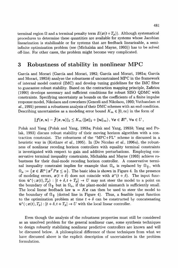
terminal region 0 and a terminal penalty term E(x(t+ Tp)). Although systematical procedures to determine these quantities are available for systems whose Jacobian linearization is stabilizable or for systems that are feedback linearizable, a semi­infinite optimization problem (see .(Michalska and Mayne, 1993)) has to be solved off-line. For other cases, the problem might become very complicated.

3 Robustness of stability in nonlinear MPC

Garda and Morari (Garda and Morari, 1982; Garda and Morari, 1985a; Garda and Morari, 1985b) analyze the robustness of unconstrained MPC in the framework of internal model control (IMC) and develop tuning guidelines for the IMC filter to guarantee robust stability. Based on the contraction mapping principle, Zafiriou (1990) develops necessary and sufficient conditions for robust SISO QDMC with constraints. Specifying uncertainty as bounds on the coefficients of a finite impulse response model, Nikolaou and coworkers (Genceli and Nikolaou, 1993; Vuthandam et al., 1995) present a robustness analysis of their DMC schemes with an end condition. Describing uncertainties as a modeling error bound Km E [0,00) in the form of

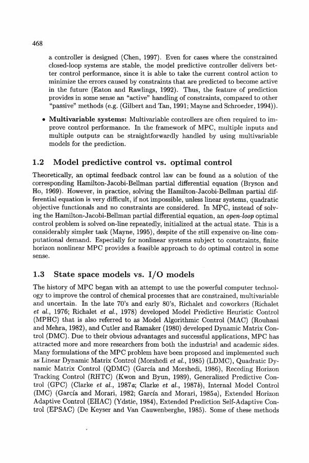
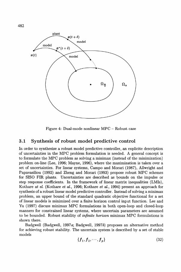
Polak and Yang (Polak and Yang, 1993a; Polak and Yang, 1993b; Yang and Po­lak, 1993) discuss robust stability of their moving horizon algorithm with a con­traction constraint. The robustness of the "MPC+FL" scheme is discussed in a heuristic way in (Kothare et al., 1995). In (De Nicolao et al., 1996a), the robust­ness of nonlinear receding horizon controllers with equality terminal constraints is investigated with respect to gain and additive perturbations. Employing con­servative terminal inequality constraints, Michalska and Mayne (1993) achieve ro­bustness for their dual-mode receding horizon controller. A conservative termi­nal inequality constraint implies for example that 0", is replaced by Oa, with

2

0", := {x E IRn I x T Px ::; Q:}. The basic idea is shown in Figure 4. In the presence of modeling errors, x(t + b) does not coincide with x*(t +.b). The input func­tion u*(·; x(t), Tp) : [t + b, t + Tp] -+ U may not steer the model to a point on the boundary of O~ but in 0"" if the plant-model mismatch is sufficiently small. The local linear feedback law u = K x can then be used to steer the model to the boundary of O~ (dotted line in Figure 4). Thus, a feasible input function to the optimization problem at time t + b can be constructed by concatenating u* (.; x(t), Tp) : [t + b, t + Tp] -+ U with the local linear controller.

Even though the analysis of the robustness properties must still be considered as an unsolved problem for the general nonlinear case, some synthesis techniques to design robustly stabilizing nonlinear predictive controllers are known and will be discussed below. A philosophical difference of those techniques from what we have discussed above is the explicit description of uncertainties in the problem formulation.

482

plant :z:(t + 6)

model

Figure 4: Dual-mode nonlinear MPC - Robust case

3.1 Synthesis of robust model predictive control

In order to synthesize a robust model predictive controller, an explicite description of uncertainties in the MPC problem formulation is needed. A general concept is to formulate the MPC problem as solving a minimax (instead of the minimization) problem on-line (Lee, 1996; Mayne, 1996), where the maximization is taken over a set of uncertainties. For linear systems, Campo and Morari (1987), Allwright and Papavasiliou (1992) and Zheng and Morari (1993) propose robust MPC schemes for SISO FIR plants. Uncertainties are described as bounds on the impulse or step response coefficients. In the framework of linear matrix inequalities (LMIs), Kothare at el. (Kothare et al., 1996; Kothare et al., 1994) present an approach for synthesis of a robust linear model predictive controller. Instead of solving a minimax problem, an upper bound of the standard quadratic objective functional for a set of linear models is minimized over a finite horizon control input function. Lee and Yu (1997) discuss minimax MPC formulations in both open-loop and dosed-loop manners for constrained linear systems, where uncertain parameters are assumed to be bounded. Robust stability of infinite horizon minimax MPC formulations is shown there.

Badgwell (Badgwell, 1997 a; Badgwell, 1997b) proposes an alternative method for achieving robust stability. The uncertain system is described by a set of stable models

(32)

483

which is assumed to contain the real plant and the nominal model used by the predictive controller. An additional robustness constraint

J i (X(t), U(·), Tp) :s; Ji (X(t), 11,(.), Tp) Vi = 1,··· ,p (33)

is introduced into the minimization problem so as to restrict the future behavior of the cost functions for all considered models. In the above, 11,(.) is a shifted version of the previous optimal input function. The feasibility of the robustness constraint leads to the plant cost function being nonincreasing, which in turn is used to show robust stability.

As a common deficiency of the nonlinear MPC schemes discussed in Section 2, disturbances and/or uncertainties either do not enter the problem formulation or they are only indirectly taken into account in that their effects are assumed to be constant over the whole prediction horizon. In the robust (linear) MPC schemes mentioned in this section, uncertainties are described either as a finite number of possible models or bounded uncertain parameters. This deficiency of MPC is exactly the strong point of 1£00 control. 1£00 theory (Ball et at., 1993; Isidori, 1995; van der Schaft, 1992) provides an excellent theoretical framework for dealing with robust stability issues. Disturbance attenuation specifications can also be incorporated very naturally into the design setup. In standard nonlinear 1£00 control, however, it is not straightforward to satisfy constraints neither on control inputs nor on disturbances.

In the purpose of combing advantages of nonlinear MPC and nonlinear 1£00 control (guaranteed robust stability and constraint satisfaction), a robust nonlinear MPC scheme that can be conceptually viewed as a combination of both methods is proposed in (Chen et at., 1997). In this robust MPC scheme, a finite horizon constrained minimax problem has to be solved on-line repeatedly and the uncertain system is described by the M - ~ structure as in 1£00 control. Thus, more general uncertainties can be considered. Moreover, uncertainties are explicitly represented in the objective functional as in 1£00 control again. In the next section, we discuss this robust nonlinear MPC scheme in a more detailed manner.

3.2 A game theoretical nonlinear model predictive control scheme

Assume that the nonlinear system under consideration is in standard affine form (that is standard in nonlinear 1£00 control)

x = a(x) + B(x)u + G(x)w, x(O) = Xo

z = [ h~) ]

(34a)

(34b)

with a(O) = 0, h(O) = 0, where u(t) E IRm is the vector of control inputs, wet) E IRP is the vector of exogenous inputs and z(t) E IRq is the vector of to-be-controlled

484

outputs. Since uncertainties and/or disturbances are represented by the exogenous inputs W, they will not be distinguished in the following. The control inputs are constrained to vary in U c IRm, where U is compact and contains 0 E IRm in its interior.

Description of uncertainties

For many practical systems, disturbances are bounded or uncertain parameters change in some region or only a set of uncertainties need to be considered. In these cases, arbitrarily time-varying uncertain parameters are usually not a good description of model-plant mismatch and may lead to overly conservative controller designs. Thus, we assume that the uncertainty enters in the nonlinear system as

W=~(x)z, (35)

where ~(x) is an arbitrary (nonlinear) smooth matrix valued function satisfying

1I~(x)11 :::; dmax (36)

and dmax < 1 is a fixed bound on the size of the uncertainty.

Example 1 As a simple example for the description of uncertainties, we consider the following nonlinear system

Xl = X2 + u(J-t + (1 - J-t)xd X2 = Xl + u(J-t - 4(1 - J-t)X2) ,

(37a)

(37b)

where the model parameter J-t is uncertain and its nominal value is 0.5. Let J-t = 0.5 + ~J-t, then the system (37) can be rewritten in form of (34a) with

a(x) = [X2] , B(x) = [ 0.5(1 + xd ] Xl 0.5(1 - 4X2)

and () [ a(1 - xd ]

G x = a(1 + 4X2) , w = ~(x)u,

where ~(x) := ~~J-t. Thus, I~J-tl < a implies 1~(x)1 < l.

The description of the uncertainty by (35) imposes constraints on the exogenous inputs that depend on the actual state of the system and on the actual control function. For a given initial condition Xo and a given control input function u(·), an exogenous input function is admissible if, along the trajectory of (34), one has

The corresponding set of exogenous input functions is denoted as W(xo, u(·».

485

Precompensation

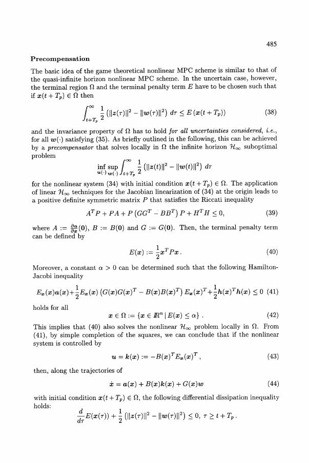
The basic idea of the game theoretical nonlinear MPC scheme is similar to that of the quasi-infinite horizon nonlinear MPC scheme. In the uncertain case, however, the terminal region n and the terminal penalty term E have to be chosen such that if x(t + Tp) E n then

1= 1 - (lIz(T)112 -lIw(T)1I2) dT ~ E (x(t + Tp))

t+Tp 2 (38)

and the invariance property of n has to hold for all uncertainties considered, i. e., for all w(·) satisfying (35). As briefly outlined in the following, this can be achieved by a precompensator that solves locally in n the infinite horizon H= suboptimal problem 1= 1

inf sup - (lIz(t)1I2 - IIw(t)1I2) dT 1.£(.) w(.) t+Tp 2

for the nonlinear system (34) w~th initial condition x(t + Tp) E n. The application of linear H= techniques for the Jacobian linearization of (34) at the origin leads to a positive definite symmetric matrix P that satisfies the Riccati inequality

(39)

where A := ~: (0), B := B(O) and G := G(O). Then, the terminal penalty term can be defined by

(40)

Moreover, a constant a > 0 can be determined such that the following Hamilton­Jacobi inequality

1 1 E",(x)a(x)+ 2E", (x) (G(x)G(xf - B(x)B(x)T) E",(xf +2h(xfh(x) ~ 0 (41)

holds for all x En: = {x E lRn I E (x) ~ a} . (42)

This implies that (40) also solves the nonlinear H= problem locally in n. From (41), by simple completion of the squares, we can conclude that if the nonlinear system is controlled by

( 43)

then, along the trajectories of

x = a(x) + B(x)k(x) + G(x)w ( 44)

with initial condition x(t + Tp) E n, the following differential dissipation inequality holds:

486

Hence, for all w (.) E W(x(t + Tp), k(x)), (44) is locally exponentially stable, n as defined in (42) is invariant and inequality (38) holds. Thus, (43) can serve as a precompensator.

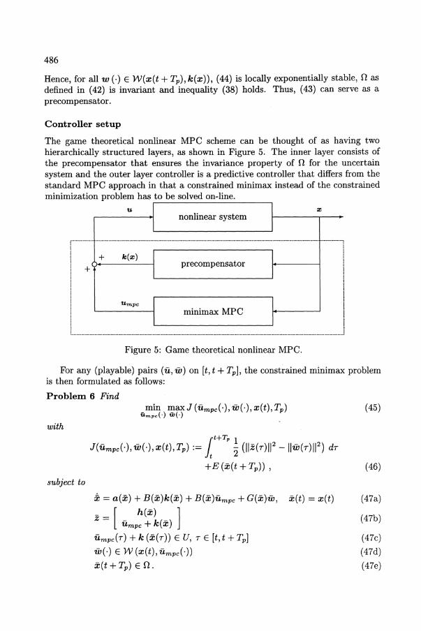
Controller setup

The game theoretical nonlinear MPC scheme can be thought of as having two hierarchically structured layers, as shown in Figure 5. The inner layer consists of the precompensator that ensures the invariance property of n for the uncertain system and the outer layer controller is a predictive controller that differs from the standard MPC approach in that a constrained minimax instead of the constrained minimization problem has to be solved on-line.

nonlinear system

,---------,--------------------------------------------------------- f-------

precompensator + k(:z:)

+

U mpc

minimax MPC

Figure 5: Game theoretical nonlinear MPC.

For any (playable) pairs (u, iiJ) on [t, t + Tp], the constrained minimax problem is then formulated as follows:

Problem 6 Find

with

subject to

x = a(x) + B(x)k(x) + B(x)umpc + G(x)iiJ, x(t) = x(t)

__ [ h(x) ] Z - umpc + k(x)

umpc(r) + k (x(r)) E U, r E [t, t + Tp)

iiJ(·) E W (x(t), u mpc (-))

x(t + Tp) En.

(45)

(47a)

(47b)

(47c)

(47d)

(47e)

487

By the invariance property of 0 and (38), the minimax predictive controller achieves that the closed-loop system satisfies the following integral dissipation inequality

S (x(tt), Tp) ~ lt2 ! (ilz(t)11 2 -llw(t)11 2 ) dt + S (X(t2), Tp) h 2

(48)

for any 0 :::; tl < h < 00 and for any admissible w(·) on [tI, h], where the function Sex, Tp) is defined by

Sex, Tp):= min max J (umpc(')' w(·), x, Tp) . u=pc(') w(.)

(49)

Under some hypotheses, it can be shown that there exists a finite time T such that for the closed-loop system x(T) E O. Then, from the robust exponential stability in 0, the closed-loop system is robustly stable. For more details see (Chen et at., 1997).

Due to the conceptual combination of nonlinear MPC and nonlinear Nco , this approach potentially combines the strong points of both methods and thus enables us to design controllers that have guaranteed robust stability and achieve good disturbance rejection properties in the face of input constraints. This scheme is however still far from a practical approach that can be recommended for and ap­plied to industrial control problems. The major obstacle at present is the high on-line computational demand which results from the solution of the constrained minimax problem. Moreover, since the precompensation is realized by a state feed­back law, originally linear input constraints will become state-dependent constraints (see (47c)), that are computationally very expensive.

4 Observer based nonlinear model predictive con­trol

All the nonlinear MPC schemes discussed previously have in common that the optimization problem will be updated with the actual system state at each sampling instance, (except for the one proposed by Genceli and Nikolaou (1995)). That is, a state feedback strategy is used. However, it is in general impossible to measure the complete system state. Thus, observer based nonlinear MPC schemes are required, where the observer is used to reconstruct the states. The difficulty here lies not only in the design of stable nonlinear observers (see for example (Gauthier and Kupka, 1994; Misawa and Hedrick, 1989)) but also in a lack of a nonlinear separation principle. Stability of the closed-loop system has to be proven in each case even if the observer and the state feedback controller are by themselves stable/stabilizing. Thus, it is not surprising that only the surface of this field has been scratched so far.

For continuous nonlinear systems, Michalska and Mayne (1995) propose a mov­ing horizon observer and discuss the stability property of the dual-mode controller with the moving horizon observer. The optimization problem of the nonlinear mov­ing horizon observer is formulated for a given past input function u(·) : [t - Te, tj -+ U as follows:

488

Problem 7 Find

with

subject to

min J (v(t - Te ), Te , y(.)) vet-Tel

J (v(t - Te ), Te , y(.)):= rt !!Y(T) - Y(T)!!2 dT it-To

:i: = f (x, u), x (t - Te) = v (t - Te) y=g(x),

(50)

(51)

(52a)

(52b)

where Te is referred to as observation horizon and y(.) on [t - Te, tl is the system measurement.

In analogy to MPC, the optimization problem (Problem 7) will be solved on-line repeatedly, updated by the new measurement. An optimal (or approximate) solu­tion (existence assumed) is denoted as v*(t - Te). If v*(t - Te) satisfies !!x(t - Te)­v*(t - Te)!! -+ a as t -+ 00, then the corresponding x*(t) is a useful estimate of x(t). The nominal convergence property of the estimated state to the true state is presented in (Michalska and Mayne, 1995). The stability property of the observer based dual-mode predictive controller is also established, where the basic idea is similar to that for achieving robustness of the dual-mode controller, namely that a conservative terminal inequality constraint is applied.

A nonlinear moving horizon state observer for discrete systems can be found in (Muske and Rawlings, 1995), where additive disturbances are also estimated and state constraints are considered in the formulation of the optimization problem.

In (Yang and Polak, 1993), closed-loop stability of the contractive nonlinear MPC scheme with a least squares estimator is discussed and in (De Oliveira and Morari, 1997), closed-loop stability of the contractive nonlinear MPC scheme with an observer designed by the extended Kalman filter technique is discussed. The advantage of the contractive nonlinear MPC approach is its exponential nominal stability. Thus, the observers reconstruct the states for the closed-loop system and the observer based contractive predictive controller is stabilizing, because of the exponential stability of the contractive controller and the locally asymptotic convergence of the observer. Clearly, initial estimation errors have to be within the convergence region of the observer.

5 Conclusions and Perspectives

In this paper we have reviewed a number of nonlinear MPC schemes, that address is­sues related to nominal or robust closed-loop stability. All of these approaches have in common that so-called stability constraints (terminal equality or inequality con­straints, contraction constraints, etc.) are introduced into the problem formulation in order to guarantee stability. Unfortunately, still neither one of these approaches

489

is completely satisfying from an application point of view. First of all, all of these ar­tificially introduced constraints certainly limit the achievable control performance and also require more or less additional on-line computational effort. Secondly, these constraints impose feasibility problems that together with the fact that all stability results are only sufficient (and not necessary), lead to a very conservative estimate for the region of attraction. Despite significant progress during the last decade there are still many open problems concerning the theoretical properties of nonlinear MPC:

• Region of attraction: As pointed out, the achieved stability is in general only local, i.e., the closed-loop system is asymptotically stable with a region of attraction that is restricted by the feasibility of the optimization problem. The latter is strongly related to the (constrained) stabilizability of nonlinear systems. For practical applications, nonlinear MPC schemes that allow for significantly enlarged operating regions are needed.

• Robustness: Despite a few results on robustness analysis of nonlinear MPC, a general theory is still lacking. With respect to synthesis of robust nonlinear predictive controllers, merely the surface has been scratched. One of the key problems in this area (that also hol.ds for non-predictive control schemes) is the formulation of suitable uncertainty descriptions.

• '!racking: In most existing nonlinear MPC schemes, the tracking problem can only be dealt with, when the required state trajectory can be calculated from the desIred (output) trajectory. Trajectory generation is an old but still challenging problem and the presence of constraints imposes additional difficulties in this respect.

• Output feedback nonlinear MPC: In practice not the whole state vector can be measured on-line. Therefore, the problem of output feedback control is essential from an application point of view. As discussed, only few preliminary stability results are known to date, and all of these results incorporate a nonlinear observer, which is very difficult to design by itself. Future advances must directly aim at deriving robustly stable output feedback schemes.

• Disturbance attenuation: At present, disturbances are only considered in a very rudimentary way in most nonlinear MPC schemes. One main goal of control is however the suppression of the effect of unknown and unmeasured disturbances, and thus nonlinear MPC schemes are needed for which distur­bance attenuation requirements can be included in the performance objective.

There are of course many more open problems related to nonlinear MPC than the ones pointed out above. Among the most important ones are the development of problem specific optimization formulations and solvers, the incorporation of identi­fication and adaptation schemes, problems related to performance monitoring and diagnosis, and the link to higher automation levels.

490

References

Allwright, J.C. and G.C. Papavasiliou (1992). On linear programming and robust model predictive control using impulse responses. Syst. Contr. Lett. 18, 159-164.

Badgwell, T.A. (1997 a). A robust model predictive control algorithm for stable linear plants. In: Proc. Amer. Contr. Conf.. Albuquerque. pp. 1618-1622.

Badgwell, T.A. (1997b). A robust model predictive control algorithm for stable nonlinear plants. In: Proc. IFAC ADCHEM. Banff. pp. 477-48l.

Ball, J.A., J.W. Helton and M.L. Walker (1993). Hoo control for nonlinear systems with output feedback. IEEE Trans. Automat. Contr. AC-38(4), 546-559.

Bitmead, R.R., M. Gevers and V. Wertz (1990). Adaptive Optimal Control - The Thinking'Man's GPC. Prentice Hall. New York.

Bryson, A.E. and Y.-C. Ho (1969). Applied Optimal Control. Ginn and Company. Waltham, Massachllsetts.

Campo, P.J. and M. Morari (1987). Robust model predictive control. In: Proc. Amer. Contr. Conf.. pp. 1021-:1026.

Chen, H. (1997). Stability and Robustness Considerations in Nonlinear Model Pre­dictive Control. Fortschr.-Ber. VDI Reihe 8 Nr. 674, VDI Verlag. Dusseldorf.

Chen, H. and F. Allgower (1996). A quasi-infinite horizon predictive control scheme for constrained nonlinear systems. In: P'roc. 16th Chinese Control Conference. Qindao. pp. 309-316.

Chen, H. and F. Allgower (1997 a). A quasi-infinite horizon nonlinear model predic­tive control scheme with guaranteed stability. Automatica. (in press).

Chen, H. and F. Allgower (1997b). A quasi-infinite horizon nonlinear predictive control scheme for stable systems: Application to a CSTR. In: Proc. IFAC ADCHEM. Banff. pp. 471-476.

Chen, H., C.W. Scherer and F. Allgower (1997). A game theoretic approach to nonlinear robust receding horizon control of constrained systems. In: Proc. Amer. Contr. Conf.. Albuquerque. pp. 3073-3077.

Clarke, D. W., C. Mohtadi and P. S. Tuffs (1987a). Generalized predictive control - Part I. The basic algorithm. Automatica 23(2),137-148.

Clarke, D. W., C. Mohtadi and P. S. Tuffs (1987b). Generalized predictive control - Part II. Extensions and interpretations. Automatica 23(2), 149-160.

Cutler, C.R. and B.L. Ramaker (1980). Dynamic Matrix Control- A computer con­trol algorithm. In: Proc. Joint Automatic Control Conference. San Francisco, CA.

De Keyser, R.M.C. and A.R. Van Cauwenberghe (1985). Extended prediction self­adaptive control. In: Proc. 7th IFAC Symposium on Identification and System

491

Parameter Estimation (H.A. Barker and P.C. Young, Eds.). Pergamon Press. Oxford. pp. 1255-1260.

De Keyser, R.M.C., G.A. Van de Velde and F.A.G. Dumortier (1988). A compara­tive study of self-adaptive long-range predictive control methods. A utomatica 24(2), 149-163.

De Nicolao, G., L. Magni and R. Scattolini (1996a). On the robustness of reced­ing horizon control with terminal constraints. IEEE Trans. Automat. Contr. 41(3),451-453.

De Nicolao, G., L. Magni and R Scattolini (1996b). Stabilizing nonlinear reced­ing horizon control via a nonquadratic terminal state penalty. In: Symposium on Control, Optimization and Supervision, CESA '96 IMACS Multiconference. Lille. pp. 185-187.

De Nicolao, G., L. Magni and R Scattolini (1997). Stabilizing receding-horizon control of nonlinear time-varying systems. In: Proc. 4rd European Control Conference ECC'97. Brussels.

De Oliveira, S.L. and M. Morari (1997). Contractive model predictive control for constrained nonlinear systems. IEEE Trans. Automat. Contr. (in press).

Doyle III, F. J., B. A. Ogunnaike and R K. Pearson (1995). Nonlinear model-based control using second-order Volterra models. Automatica 31(5), 697-714.

Eaton, J. W. and J. B. Rawlings (1992). Model predictive control of chemical pro­cesses. Chem. Eng. Sci. 47(4), 705-720.

Findeisen, RH. and J.B. Rawlings (1997). Suboptimal infinite horizon nonlinear model predictive control for discrete time systems. NATO Advanced Study In­stitute on Nonlinear Model Based Process Control.

Garda, C.E. and A.M. Morshedi (1986). Quadratic programming solution of dy­namic matrix control (QDMC). Chem. Eng. Commun. 46, 73-87.

Garda, C.E. and M. Morari (1982). Internal Model Control. 1. A unifying review and some new results. Ind. Eng. Chem. Process Des. Dei!. 21,308-323.

Garda, C.E. and M. Morari (1985a). Internal Model Control. 2. Design procedure for multivariable systems. Ind. Eng. Chem. Process Des. Dev. 24,472-484.

Garda, C.E. and M. Morari (1985b). Internal Model Control. 3. Multivariable con­trol law computation and tuning guidelines. Ind. Eng. Chem. Process Des. Dev. 24, 484-494.

Garda, C.E., D.M. Prett and M. Morari (1989). Model Predictive Control: Theory and practice - A survey. Automatica 25, 335-347.

Gauthier, J.P. and LA.K. Kupka (1994). Observability and observers for nonlinear systems. SIAM J. Cantr. Optim. 32(4), 975-994.

Genceli, H. and M. Nikolaou (1993). Robust stability analysis of constrained L 1-

norm model predictive control. AIChE J. 39(12), 1954-1965.

492

Genceli, H. and M. Nikolaou (1995). Design of robust constrained model-predictive controllers with Volterra series. AIChE J. 41(9), 2098-2107.

Gilbert, E.C. and K.C. Tan (1991). Linear systems with state and control con­straints: The theory and application of maximal output admissible sets. IEEE Trans. Automat. Contr. AC-36, 1008-1020.

Hovd, M., J.H. Lee and M. Morari (1993). Truncated step response models for model predictive control. J. Proc. Contr. 3(2), 67-73.

Isidori, A. (1995). Hoc control via measurement feedback for general nonlinear sys­tems. IEEE Trans. Automat. Contr.

Keerthi, S.S. and E.G. Gilbert (1988). Optimal infinite-horizon feedback laws for a general class of constrained discrete-time systems: Stability and moving­horizon approximations. J. Opt. Theory and Appl. 57(2), 265-293.

Kleinman, D.L. (1970). An easy way to stabilize a linear constant system. IEEE Trans. Automat. Contr. AC-15, 692.

Kothare, M. V., V. Balakrishnan and M. Morari (1996). Robust constrained model predictive control using linear matrix inequalities. Automatica 32(lO), 1361-1379.

Kothare, M.V., V. Balakrishnan and M. Morari (1994). Robust constrained model predictive control using linear matrix inequalities. In: Proc. Amer. Contr. Conf.. Baltimore, Maryland. pp. 440-444.

Kothare, M.V., V. Nevistic and M. Morari (1995). Robust constrained model pre­dictive control for nonlinear systems: A comparative study. In: Proc. 34th IEEE Conf. Decision Contr .. New Orleans, LO. pp. 2884-2885.

Kurtz, M.J. and A. Henson (1996). Linear model predictive control of input-output linearized processes with constraints. In: 5th International Conference on Chemical Process Control - CPC v.

Kwon, W.H. and D.G. Byun (1989). Receding horizon tracking control as a predic­tive control and its stability properties. Int. J. Contr. 50(5), 1807-1824.

Lee, J. H., M. Morari and C.E. Garcia (1994). State-space interpretation of model predictive control. Automatica 30(4),707-717.

Lee, J.H. (1996). Recent advances in model predictive control and other related areas. In: 5th International Conference on Chemical Process Control - CPC v.

Lee, J.H. and Z.-H. Yu (1997). Worst-case formulations of model predictive control for systems with bounded parameters. Automatica 33(5), 763-78l.

Maner, B. R., F. J. Doyle III, B. A. Ogunnaike and R. K. Pearson (1994). A nonlinear model predictive control scheme using second order Volterra models. In: Proc. Amer. Contr. Conf.. Baltimore, Maryland. pp. 3253-3257.

493

Mayne, D. Q. (1995). Optimization in model based control. In: Proc. IFAC Sympo­sium Dynamics and Control of Chemical Reactors, Distillation Columns and Batch Processes. Helsingor. pp. 229-242.

Mayne, D. Q. (1996). Nonlinear model predictive control: An assessment. In: 5th International Conference on Chemical Process Control - CPC V.

Mayne, D. Q. and H. Michalska (1990). Receding horizon control of nonlinear sys­tems. IEEE Trans. Automat. Contr. AC-35(7), 814-824.

Mayne, D. Q. and W. R. Schroeder (1994). Nonlinear control of constrained linear systems. Int. J. Contr. 60(5), 1035-1043.

Meadows, E.S., M.A. Henson, J.W. Eaton and J.B. Rawlings (1995). Receding horizon control and discontinuous state feedback stabilization. Int. J. Contr. 62(5), 1217-1229.

Michalska, H. and D.Q. Mayne (1991). Receding horizon control of nonlinear sys­tems without differentiability of the optimal value function. Syst. Contr. Lett. 16, 123-130.

Michalska, H. and D.Q. Mayne (1993). Robust receding horizon control of con­strained nonlinear systems. IEEE Trans. Automat. Contr. AC-38(1l), 1623-1633.

Michalska, H. and D.Q. Mayne (1995). Moving horizon observers and observer-based control. IEEE Trans. Automat. Contr. AC-40(6), 995-1006.

Misawa, E.A. and J.K. Hedrick (1989). Nonlinear observers - a state-of-the-art survey. ASME J. Dyn. Syst. Meas. Cntrl. 111,344-352.

Morari, M. and J.H. Lee (1991). Model predictive control: The good, the bad, and the ugly. In: Proc. 4th International Conference on Chemical Process Control - CPC IV (Y. Arkun and W. Ray, Eds.). AIChE, CACHE. TX. pp. 419-444.

Morshedi, A.M., C.R. Cutler and T.A. Skrovanek (1985). Optimal solution of dy­namic matrix control with linear programming techniques (LDMC). In: Proc. Amer. Contr. Conf.. pp. 199-208.

Muske, K.R. and J.B. Rawlings (1995). Nonlinear moving horizon state estimation. In: Methods of Model Based Process Control (R. Berber, Ed.). pp. 349-365. Kluwer Academic Publishers. Netherlands.

Nevistic, V. and M. Morari (1995). Constrained control of feedback-linearizable systems. In: Proc. 3rd European Control Conference ECC'95. Rome. pp. 1726-1731.

Polak, E. and T.H. Yang (1993a). Moving horizon control of linear systems with input saturation and plant uncertainty. Part 1. Robustness. Int. J. Contr. 58(3),613-638.

Polak, E. and T.H. Yang (1993b). Moving horizon control of linear systems with input saturation and plant uncertainty. Part 2. Disturbance rejection and track­ing. Int. J. Contr. 58(3),639-663.

494

Qin, S.J. and T.A. Badgwell (1996). An overview of industrial model predictive con­trol technology. In: 5th International Conference on Chemical Process Control - CPC V.

Rawlings, J.B. and K.R. Muske (1993). The stability of constrained receding horizon control. IEEE Trans. Automat. Contr. AC-38(10), 1512-1516.

Rawlings, J.B., E.S. Meadows and K.R. Muske (1994). Nonlinear model predictive control: A tutorial and survey. In: Proc. ADCHEM'94. Kyoto, Japan.

Richalet, J. (1993). Industrial applications of model based predictive control. Au­tomatica 29(5),1251-1274.

Richalet, J., A. Rault, J.1. Testud and J. Papon (1976). Algorithmic control of in­dustrial processes. In: Proc. 4th IFAC Symposium on Identification and System Parameter Estimation. Tbilisi. pp. 1119-1167.

Richalet, J., A. Rault, J.L. Testud and J. Papon (1978). Model predictive heuristic control: Application t? industrial processes. Automatica 14, 413-428.

Ricker, N.L. (1991). Model predictive control: State of the art. In: Proc. 4th Inter­national Conference on Chemical Process Control - CPC IV (Y. Arkun and W. Ray, Eds.). AIChE, CACHE: TX. pp. 271-296.

Rouhani, R. and R.K Mehra (1982). Model algorithmic control (MAC): Basic the­oretical properties. Automatica 18(4), 401-414.

Scokaert, P.O.M. and J.B. Rawlings (1996). Infinite horizon linear quadratic control with constraints. In: Proc. 13th IFAC World Congress. Vol. M. San Francisco. pp. 109-114.

van der Schaft, A.J. (1992). L2-gain analysis of nonlinear systems and nonlinear state feedback HOC) control. IEEE Trans. Automat. Contr. AC-37(6), 770-784.

Vuthandam, P., H. Genceli and M. Nikolaou (1995). Performance bounds for robust quadratic dynamic matrix control with end condition. AIChE J. 41(9), 2083-2097.

Yang, T.H. and E. Polak (1993). Moving horizon control of nonlinear systems with input saturation, disturbances and plant uncertainty. Int. J. Contr. 58(4),875-903.

Ydstie, B.E. (1984). Extended horizon adaptive control. In: Proc. 9th IFAC World Congress (J. Gertler and 1. Keviczky, Eds.). Pergamon Press. Oxford. pp. 911-915.

Zafiriou, E. (1990). Robust model predictive control of processes with hard con­straints. Compo fj Chem. Eng. 14(4/5), 359-37l.

Zheng, A. and M. Morari (1993). Robust stability of constrained model predictive control. In: Proc. Amer. Contr. Con/.. pp. 379-383.