1

IRES2011-002

IRES Working Paper Series

Nonlinear Modelling of the Highest and Best Use in the Valuation of Mixed-Use

Development Sites

Kwame Addae-Dapaah Kim-Chuan Toh

January, 2011

2

Nonlinear Modelling of the Highest and Best Use in the Valuation of Mixed-Use Development Sites

Kwame Addae-Dapaah*

Kim-Chuan Toh**

* Department of Real Estate, School of Design & Environment, NUS, Singapore.

** Department of Mathematics, Faculty of Science, NUS, Singapore.

Correspondence to:

Kwame Addae-Dapaah

Department of Real Estate

National University of Singapore

4 Architecture Drive

Singapore 117566

Tel: (65) 6516 3417 Fax: (65) 6774 8684

E-mail: rstka@nus.edu.sg

JEL Classification Code: C61, G12

3

Nonlinear Modelling of the Highest and Best Use in the Valuation of Mixed-Use Development Sites Abstract The valuation of any mixed-use development site must perforce grapple with the allocation of

the site to the permitted uses as market valuation is premised upon highest and best (HBU) use.

The optimization problem involved in such cases prejudices the sole use of traditional valuation

methods which cannot deal with the inherent allocation problem. Furthermore the synergism

among the permissible uses introduces more complexities to the problem. Thus, the assumption

of a linear relationship among the permissible uses may not suffice; neither is it intuitively

appealing – A nonlinear model is used to resolve the optimization problem involved in the

exercise before valuing the site via the Residual method. While the nonlinear model allocates the

site to all six permissible uses, the linear model allocates the site to five of the uses. Furthermore,

the nonlinear model results in a gross development value and a site value that are 22.04% and

39.81% respectively higher than the linear model.

Key words: Mixed-use development, synergy, management science, valuation, residual method.

1. Introduction

The quest for sustainable real estate, as a result of the sustainability movement, is providing

more impetus for mixed-use developments. Although there is ample literature on the concept of

highest and best use (e.g. Graaskamp 1970, North 1981, Grissom 1983, Lennhoff 1995, Sarazen

1995, Wilson 1995 & 1996 and Finch 1996) the extant literature mainly focuses on various

aspects of highest and best among competing alternate uses (see Addae-Dapaah). Apart from

Gau and Kohlhepp (1980), Winokur et al. (1981), Peiser and Andrus (1983), Mouchly and Peiser

(1993) and Addae-Dapaah (2005), the extant literature does not deal with the complex issue of

ascertaining the best mix of uses (as may pertain to a mixed-use development site) that

maximizes return, and thus, constitutes the highest and best “use” (HBU).

Gau and Kohlhepp (1980) use linear programming to generate a development/construction

schedule which maximizes the profitability of a real estate project. Winokur et al. (1981) employ

4

linear programming to propose a land development strategic plan that maximizes the expected

present value of the future cash flows of a real estate development project. Furthermore, Peiser

and Andrus (1983) utilize integer programming to schedule office construction while Mouchly

and Peiser (1993) use linear programming to deal with optimal land use plan. However, none of

these studies relates to valuation of the site. Given that some of these mixed-use development

sites are aimed at giving the prospective developer maximum flexibility in choosing the “best”

permissible single, or mix of, use(s), a valuer must ideally ascertain the best mix of uses that

promotes both efficient land utilization and maximization of profits to underpin the valuation of

the site.

Mixed-use development sites are normally offered for sale in areas where there are no market

value/rental data for development land. Therefore valuers appropriately rely on the Residual

method and/or cash flow analysis for valuing such sites. Addae-Dapaah (2005) finds that the

usefulness of the Residual method for valuing a mixed-use development site could be severely

compromised as the method, and even the much trumpeted cash flow method, per se cannot

resolve the inherent optimization problem in the valuation of a mixed-use development site.

Furthermore, Addae-Dapaah (2005) observes that studies that use the real option model to

explain the valuation of land and factors affecting investment decisions, such as Titman (1985),

Capozza and Hesley (1990), Williams (1991), Grenadier (1995) and Paxson (2005) deal with the

option in relation to a single use rather than a mix of uses. Moreover, all the studies that utilize

artificial neural network (ANN) for real estate appraisal (e.g. Tsukuda and Baba, 1990; Do and

Grudnitski, 1992; Tay and Ho, 1992; Allen and Zumult, 1994; Worzala et al., 1995; Bagnoli et

al., 1998; Nguyeh and Cripps, 2001; Peterson and Flanagan, 2009) relate to single use

developments or sites that are already developed rather than sites that can be put to a mix of uses.

Geltner et al. (1996) deal with the choice between two underlying assets rather than a choice

among several independent alternate uses or mix/different mixes of uses, whichever maximizes

return. Similarly, Capozza and Li (1994), inter alia, deal with the conversion of vacant land to

urban use vis-à-vis price of the land as a function of option premium. The extant literature on

fuzzy logic and ANN vis-à-vis property valuation, in addition to providing us with conflicting

views on the relative performance of both soft computing approaches and the hedonic model,

5

deals with the nonlinearity between the value of a home and some of the factors affecting

property value as well as the predictive power of ANN (see for example, Grether and

Mieszkowski, 1974; Do and Grudnitski, 1993; Goodman and Thibodeau, 1995; Liu et al., 2006;

Lam et al., 2008; Peterson and Flanagan, 2009). The extant literature on soft computing does not

deal with valuation of mixed-use properties which involve optimizing the allowable uses.

However, with the development of the multi-layered perception, soft computing is capable of

handling optimization problems (Lee and Paik, 2006) and thus, deal with the problem inherent in

the valuation of a mixed-use development site provided there is sufficient market data for the

training involved in ANN.

Addae-Dapaah (2005) appears to be the only researcher who has used the linear programming

(LP) model to find the mix of uses that maximizes return for a mixed-use development site.

However, Addae-Dapaah (2005) assumes that the values for the permitted land uses encapsulate

the synergy among the related uses to justify the LP model. While this is plausible, it must be

noted that some mixed-use developments occur in areas where it is almost impossible to find

analogs that encapsulate the synergy that a proposed mixed-use development will generate. For

example, the “white site”, a novel form of mixed-use development sites, which Addae-Dapaah

(2005) uses for his study, was reclaimed from the sea. There were no acceptable analogs (when

“white sites” were first offered for sale) to justify the assumption that the values capitalized the

synergism of the related land uses. This implies that Addae-Dapaah’s (2005) study that is

premised on the assumption of linear relationships among the permissible land uses and their

values could be simplistic – A nonlinear model that accounts for the synergy among the alternate

competing uses may be more appropriate.

Thus, a gap exists in the literature on the mix of uses (allocation problem) that maximizes return

(which accounts for the synergy among the various land uses) for a mixed-use development site

to constitute the HBU. This gap may be filled by utilizing soft computing – a collection of

methodologies that work synergistically to provide information processing capabilities for

handling real-life situations (Sethuraman, 2006). According to Jain et al. (1996: ), the Hopfield

network can be used to find the optimal (or suboptimal) solution if a combinatorial optimization

problem, such as the classical travelling salesman problem, can be formulated in terms of

6

minimizing network energy function. However, ANN may be unsuitable for the current task as it

requires market data (which are not available) for training – Mixed-use development sites often

do not have analogs to provide the required data for training ANN. Furthermore, Sethuraman

(2006:203) states: “Currently, fuzzy logic (Wang, 1997), artificial neural networks (Hassoun,

1995; Mehrotra et al., 1997) and genetic algorithms (Everitt and Dunn, 2001) are three main

components of soft computing. ANN is suitable for building architectures for adaptive learning,

and GA can be used for search and optimization. Fuzzy logic provides methods for dealing with

imprecision and uncertainty. The analytical value of each one of these tools depends on the

application”. Given the inability of fuzzy logic and ANN to explain their behaviour (Sethuraman,

2006) and that many design parameters still have to be determined by the trial-and-error method

(Jain et al., 1996), LP and nonlinear programming (NLP), with their shadow pricing, Lagrange

multipliers, active and inactive constraints etc., appear to be more suitable than fuzzy logic and

ANN in the valuation of mixed-use development site. Our bias is tilted towards LP/NLP. Thus,

this study attempts to fill the gap (and therefore contributes to existing literature) by utilizing LP

and NLP to model the HBU for a mixed-use development site to show that the NLP model

provides better results which, combined with Residual or any traditional method of valuation,

will produce a more scientifically based and supportable estimate of value for a mixed-use

development site.

The study is organized as follows. A mixed-use development site and the attendant valuation

problems are briefly discussed. This is followed by a theoretical development of the problem in

the context of management science. The sections that follow cover methodology and data

sourcing and management, empirical modelling of the HBU, presentation and interpretation of

the results, and a valuation of a mixed-use development site in Singapore. It is concluded that the

use of linear programming model to value a mixed-use development site could be problematic as

the nonlinear model (which accounts for synergy among the uses) result in a gross development

value and site value that are 22.04% and 39.81% higher than those of the linear model.

2. Mixed-use Development Site and the HBU Puzzle in Valuation

The HBU puzzle involved in the valuation of a mixed-use development site, and the similarities

and differences between a traditional mixed-use and “white site” have been articulated by

7

Addae-Dapaah (2005). The peculiar feature of a “white site” is the maximum flexibility offered

to the owner to put the site to any single use or mix of the permissible uses, and change the

use/mix of uses whenever he deems fit without recourse to the planning authority.

Therefore the owner of the site has the problem of allocating scarce resources (e.g. land, money,

etc.) among alternate competing uses at different times to maximize his profit subject to

financial, technological and institutional constraints that limit his prerogatives – the owner of the

site has “constrained” options. Thus, option pricing could lend itself to the valuation of such sites

albeit the Residual valuation and discounted cash flow valuation being the norm in Singapore.

Addae-Dapaah (2005) argues that both the Samuelson-McKean (1965) method for valuing

vacant land and the Residual method of valuation are premised on the HBU of the land.

Furthermore, it is argued that the two models presume, rather than resolve, the HBU problem

which the valuation of “white sites” (and any mixed-use development site) poses (Addae-Dapaah

2005). Similarly, cash-flow-based valuation is based on HBU which is presumed. The

computations involved in ascertaining the highest and best use or mix of uses (HBMU) that will

maximize utility (i.e. land value) given the institutional, economic, physical and technological

constraints of a particular “white site” that permits residential, retail, restaurant, office, hotel and

Cineplex developments or any combination thereof could be numerous, while the calculations

involved in a trial-and-error method could be tedious and quite inefficient in terms of time and

cost.

3. Relevance of Management Science

The brief discussion on “white site” and valuation reveals that optimization (i.e. combining the

permissible land uses to produce the highest return) is pivotal to the valuation of a mixed-use

development site. The complexity of the problem is compounded by the fact that the land value

attributable to each use is inextricably intertwined with the other permissible uses because of the

synergy that exists among the uses. Furthermore, the actions of whoever owns the site are

constrained by political, social, economic, planning etc. obligations. Thus, apart from physical

(plot size, and land use capacity and intensity), resources and planning limitations on the site’s

development, a developer has to grapple with the following two challenges if he is to maximize

returns (see Addae-Dapaah, 2005):

8

a) The permissible economic use(s) to be developed given that some, or all, of these

uses could be functionally complementary or incongruous to have synergistic

effect(s); and

b) Marginal revenue and opportunity cost attributable to each permissible economic use.

The marginal revenue for each use could be affected by the marginal revenue(s) of

other use(s) because of the synergism among the permissible uses. This makes the

combination of the uses very challenging as the synergism among the permissible

uses can have either positive or negative impact on the associated marginal revenues

and opportunity costs.

In addition, the prevalence of institutional, financial, physical, etc. constraints calls for complex

trade-offs among the variables associated with a mixed-use development site. As noted by

Winokur et al. (1981:50), “Management Science techniques are particularly well suited to

handling such complex trade-offs systematically, in a manner which presents and evaluates

alternatives for management”. Since the valuation exercise primarily centres on the allocation of

a scarce resource (i.e. land) among alternate competing uses and different mixes thereof,

management science (in particular LP and NLP) would appear to be the best analytical tool

before utilizing the appropriate valuation method(s) to estimate the value of the site.

4.1 Methodology

The LP and NLP models are employed to resolve the allocation problem in the case before

applying the Residual method to value the site. The LP and NLP models can be expressed as the

minimization/maximization of a (non)linear function subject to (non)linear inequality and/or

equality constraints (Rardin 1998; Carter and Price 2001; Avriel, 1976). Both models may

generally have three fundamental variables: a finite number of real variables (land use in our

case), a finite number of constraints (e.g. resource availability and institutional controls) which

the variables must satisfy, and a function of the variables which must be maximized/minimized

(i.e. land value/cost in our case). In mathematical terms, we are finding specific values ( )nxx ,...,1 ,

if they exist, of the variables ( )nxx ,...,1 that will satisfy:

Maximize/minimize

θ ( )nxx ,...,1 (1)

9

subject to:

( ) 0,...,1 ≤ni xxg ; i = 1,…, m (2)

( ) 0,...,1 =nj xxh ; j = 1,…, k (3)

where θ, gi and hj are numerical functions of the variables x1, …, xn, which represent the

permissible economic land uses (e.g. condominium, retail, etc.). θ depicts the marginal revenue

(i.e. value per m2) associated with the corresponding permissible economic land uses.

Alternatively, θ may be construed as the opportunity cost for not putting the site to the relative

uses. If the functions θ, gi and hj are linear in the variables x1,…, xn, then the optimization problem

(1)-(3) is known as a linear program; otherwise, it is classified as a nonlinear program (Avriel,

1976).

4.1.1 Differences between LP and NLP

LP and NLP problems differ in model specification and level of difficulties in solving problems.

Although both models generally have three fundamental variables as explained above, one main

difference between LP and NLP is that a NLP can have a nonlinear objective function and/or one

or more nonlinear constraints (Ragstale, 2001). Secondly, LP problems can be solved with

relative ease compared to NLP problems because:

a. LP problems lend themselves to “corner” or extreme point solutions. Given any

bounded LP problem, it is certain that one “corner” or extreme point of the feasible

solution is optimal. (Thus, in principle, it is only necessary to search over a finite

number of feasible solutions – extreme points – to solve an LP problem, but one

should note that such an exhaustive search is computationally impractical as there is

exponential number of extreme points.) The Simplex method, originally proposed by

G. Dantzig, can efficiently solve LPs with hundreds of variables and constraints. It

takes advantage of the extreme-point property of the optimal solution by traversing

from extreme point to extreme point to improve on the optimality of the solution.

b. An extreme point, which provides an objective function value that cannot be

improved by any movement away from it, must and is the optimal solution to the

problem. In other words, any locally optimal solution (i.e. a solution that is better than

any other feasible solution in its immediate, or local, vicinity) must also be the

optimal over the whole feasible region (i.e. global optimal).

10

In contrast, NLPs do not generally have the above beneficial properties of LPs. NLPs do not

generally have extreme point solutions. This implies that there is no analogue of the Simplex

method for solving a NLP. A variety of sophisticated methods relying on local linear/quadratic

function approximations to iteratively solve a NLP problem are currently available as a result of

the great advances in the optimization community in the past three decades. However, these

methods would usually take more computing time to solve a NLP compared to the Simplex

method on a LP with the same number of variables and constraints. Apart from computational

tractability, the challenge in solving a NLP is compounded by the fact that NLPs could have

local optima that might not be overall optimal. Thus, one should ideally find all the local optima

in NLPs to be able to ascertain the overall optimum. This sharply contrasts with LPs which are

solved once a local optimum is found.

Another problem that can arise in NLP is the possibility for the feasible region to have two or

more entirely disconnected sets of points. Thus, any “generalized reduced gradient” or “path

following algorithm (as pertains in the simplex method for solving LPs) may not enable us to

find the overall optimal solution as the algorithm cannot cross from one segment of a

disconnected feasible region to another. The problem is essentially the same as that which can

emanate from the existence of different local optima in a fully connected feasible region – The

local optimum solution at which a “path-following” algorithm terminates depends almost

entirely on the initial starting point (see Simmons, 1975; Bertsekas, 1995; Ragsdale, 2001).

These difficulties in NLPs are dealt with systematically based on duality theory, and Lagrange

Multipliers and Kuhn-Tucker theory. Lagrange Multipliers deal with unconstrained and equality

constrained problems while Kuhn-Tucker optimality theory (Kuhn and Tucker, 1951) is the

theoretical underpin for virtually all the solution methods of NLP (Simmons, 1975; Bazaraa &

Shetty, 1990).

4.1.2 Kuhn Tucker Conditions

To give the reader an idea of the Kuhn Tucker optimality theory, we consider the following NLP

without equality constraints:

Max f(X) X = (x1…xn)

11

s.t. gi(X) ≤ 0, i = 1, 2, …, m

X ≥ 0,

where the functions f(X), gi(X) are assumed to be continuously differentiable in the feasible

region. The nonlinear HBU model which we shall study in Section 4.2 has exactly the above

form, where f(X) is a nonlinear function but gi(X) are all linear functions. The most general form

of NLP stated in (1)—(3) is beyond the tenet of this paper, and we refer interested readers to see

for example: Bazaraa and Shetty, 1990; Ragsdale, 2001; Kasana and Kumar, 2004 for detailed

explanation.

The necessary conditions for to be a local optimal solution of the problem are:

(4)

(5)

(6)

where is the Lagrange function: .

Equations (4)-(6) are the Kuhn-Tucker (K-T) necessary conditions for optimality. Except for rare

pathological cases, it means that any local optimal solution X* of the NLP can be found among

the solutions satisfying the K-T necessary conditions. There are sufficient conditions (known as

K-T second order sufficient conditions, see Bazaraa and Shetty, 1990; Kasana and Kumar, 2004)

to determine which K-T solutions are local maxima which we shall not present here for brevity.

As the name suggests, a local maximizer X* is a point in the feasible region of the NLP which

gives the largest objective function value among points in a local vicinity of X*. If X* also gives

the largest objective function value among all the feasible points of the NLP, it is also called a

global maximizer. As stated in Simmons (1975:201), if the functions -f(X), gi(X) are all convex

functions in the feasible region, then any local maximizer is also a global maximizer.

4.2 Data Sourcing and Management

Data for modelling the LP/NLP problem were mainly obtained from the tender document for the

white site used as a case study for the paper, Real Estate Information System (REALIS), Rider

12

Hunt and Bailey (RHB – a cost consulting firm in Singapore), and property consulting firms in

Singapore. REALIS is an URA database, which records open market sale prices obtained from

caveats lodged with Singapore Land Authority (i.e. Registrar of Title Deeds). The data are

updated fortnightly on the first and sixteenth of every month. REALIS is the most reliable public

database that is used by property market researchers in Singapore. The relevant inputs for

modelling the allocation problem [equations (1)-(3)] are the cost and expected values per unit of

the permissible land uses (assuming the land is fully developed) as well as the impact of the

synergy among these land uses on the corresponding land values. The fact that the price of land

in Singapore is a function of the plot ratio (i.e. building-to-land ratio) vis-à-vis a plot ratio of 6.0

as implied by the land area of 26,667.9 m and a maximum gross floor area (GFA) of 160,016 m²,

suggests that a high-rise development, as opposed to low-density development of detached

houses, etc. is more suited to the site. Thus, the most suitable residential development (which

conforms to, or balances existing developments in the surrounding areas) that is used for

modelling the problem is condominium. In addition, the planning guidelines for the site permit

commercial, entertainment and hotel uses. Moreover, information from REALIS and the industry

reveals that the mean value (reflecting the long term occupancy and absorption rates, etc.) and

cost per m2 of the permissible land uses are as follows:

Land Use Value per m2 Cost per m2

Condominium (x1) r1 = S$12,2001 c1 = S$4,500

Retail (x2) r2 = S$18,840 c2 = S$4,350

Office (x3) r3 = S$10,760 c3 = S$3,950

Hotel (x4) r4 = S$13,750 c4 = S$5,650

Restaurant (x5) r5 = S$13,078 c5 = S$4,350

Cineplex (x6) r6 = S$ 15,850 c6 = S$3,000

The cost per m2 (obtained from RHB and the industry) includes professional fees and financing

cost but excludes land cost. Similarly, the values per m2 are based on sale prices of comparable

properties extracted from REALIS, and from the industry.

The residential, retail and office developments are each divided into two categories as shown in

the definition of the decision variables (land uses) under the sub-section 4.2.1 “Empirical

13

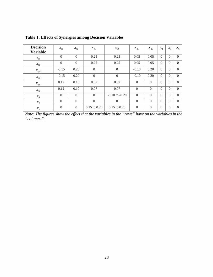
Modelling of the Problem”. The figures in Table 1, which are extracted from a study by Teo

(2006), in which 2000 sale transactions were examined in an attempt to quantify the impact of

mixed-use developments on the value of the various uses, and data from property consultancy

firms in Singapore, depict the impact of the synergism among the decision variables (land uses)

on the values of the respective decision variables. For example, ax1 and bx1 (residential

developments) increase the values of retail and office developments by 25% and 5%

respectively. Similarly ax2 and bx2 reduce the values of ax1 and ax3 by 15% and 10%

respectively and increases the values of both bx1 and bx3 by 20%.

Table 1

In addition to the above, information from the industry indicates that retail development requires

a minimum GFA of 5,000m2 in a mixed-use development to make it viable. Similarly, given the

configuration of comparable Cineplex in Singapore, Cineplex in the proposed development

should occupy at least a floor area of 1,000 m² (Equation (13)), and we assume the maximum

floor area of 3,000 m² (Equation (14)). Other relevant data for modelling the problem are

obtained from a white site in Singapore. The relevant features of the planning guidelines are as

follows:

Land Use: White site – commercial/residential/hotel uses.

Gross Floor Area: The maximum permissible GFA is 160,016 m² of which at least 40% and

15% must be for office and hotel uses respectively. The remainder of the maximum permissible

GFA (45%) may be used for any one or more of the following uses – commercial (e.g. office,

retail and entertainment), hotel, residential.

In LP and NLP language, the minimum and maximum GFA figures are resource constraints.

Furthermore, restaurants in shopping malls in Singapore are classified as retail – A portion of the

retail area is used for restaurants. A shopping complex in Singapore has been allowed to use a

maximum of 24% of the retail area for food and beverages (F&B). To encourage retail mix, we

assume that at least 20% of the retail space must be used for F&B (Equation (15)).

14

In view of all these information, the total cost of a mixed-use development, which takes account

of the mandatory minimum GFA requirements and assuming that the remaining GFA is equally

allocated among the permissible uses is “S$719,259,550”2 (see Addae-Dapaah 2005). This basis

of calculating the total cost of the development is necessary to provide an initial basis for

analysis as the optimal allocation of the GFA to the various uses is not known yet. Furthermore,

total cost based on the mandatory minimum GFA requirements and allocating the remaining

GFA to the most profitable permissible use (retail) assuming the market can absorb it

(S$701,670,160), is lower than the former. Given that the latter figure does not fully account for

all the synergism among the permissible uses while setting a lower bound on funds required for

the project, the former figure which is based on all the permissible uses and thus, facilitates

capitalization of the synergism among the uses appear to be more pragmatic and reasonable in

our case where the optimal solution is yet to be ascertained. Thus, the problem is finding the use

or mix of uses (and in what proportion) that will maximize the return from the development on

the basis of the given information.

4.2.1 Empirical Modelling of the Problem

The data in the preceding subsection are used to model the HBU/HBMU problem as follows.

4.2.1.1 NLP Model

Define the following decision variables:

=ax1 Total floor area of residential development located right next to retail development The retail use is thus a negative externality.

=bx1 Total floor area of residential development located near to retail development – This category is at a “safe” distance from the retail. Proximity to the retail development has favourable effect on the value of this category of residential development.

=ax2 Total floor area for retail use (excluding restaurant) in shopping mall.

=bx2 Total floor area of retail development (excluding restaurant) adjoining hotel development.

=ax3 Total floor area of office development located right next to retail development and/

15

or share the same entrance. Retail development is a negative externality to the office space.

=bx3 Total floor area of office development located near to retail development – Office space is located at a congenial distance. Retail development becomes an amenity and thus favourably impacts the value of the office space.

=4x Total floor area of hotel development.

=5x Total floor area of restaurant development.

=6x Total floor area of Cineplex development. Maximize

( )( )( )( ) ( )( ) ( )( ) 666555444333

333222222111111

111))(1(

))(1(1))(1())(1())(1(

xxdrxxdrxxdrxxdrxxdrxxdrxxdrxxdrxxdr

bb

aabbaabbaa

++++++++

+++++++++ (7)

subject to the following constraints:

0,..., 61 ≥xx

where

850,15,078,13,750,13,760,10,840,18,220,12 654321 ====== rrrrrr000,3,350,4,650,5,950,3,350,4,500,4 654321 ====== cccccc ;

16

where 2.02 =κ , 1.03 =κ ,

where Note: one can also model the effect of oversupply of retail or office space by modifying the d’s in the above model3. The functions d1a(x),…, d6(x) represent the fractional adjustments to the nominal returns

r1,…,r6 of the properties x1a,…,x6 when the synergistic effects of a mixed-use development are

taken into account. We model the return adjustment to a particular land use to be dependent on

the floor areas of the other land uses in a concave manner as specified by the functions in (22)-

(23). The function g3(t) is chosen such that its value is equal to 1 when t = 40,004, i.e., when the

total office area reaches 40,004 m², its contributions to the return adjustments on other properties

reach the values given in Table 1. Similar explanations hold for the functions g1(t), g2(t) and

g4(t). The value of 40,004 was obtained by assuming that the return adjustments given in Table 1

are based on dividing the GFA uniformly among the 4 major types of properties: retail,

residential, office, and hotel. The function g6(t) associated with the Cineplex development is

chosen such that its value is equal to 1 when t reaches the minimum stipulated area of 1000 m².

4.2.1.2 LP Model

Maximize

654333322221111 rrrxrxrxrxrxrxr bababa ++++++++ (24) subject to the constraints in equations (8) – (15).

Both the LP and NLP models have the same constraints (equations 8-15). The main difference

between the two models lies in the objective functions (equations 7 and 24). The objective

17

function for the LP model assumes either linear relationships among the related land uses or that

the effect of any synergy among the land uses is encapsulated in r1,…r6 (i.e. the value per m2 of

the land uses. The probability of r1,…,r6 reflecting the synergism of the land uses of a “white

site” (as suggested by Addae-Dapaah, 2005) is very low as there was no acceptable analog for

“white sites” at the time they appeared on the market. Moreover, notwithstanding the

development of a few “white sites” in Singapore over the past few years, they markedly differ in

location and permitted land uses to permit any meaningful comparison to extract r1,…,r6 that

reflect the synergism of the land uses. Thus, the effects of the interactions among the land uses

d1a(x),…,d6(x) – equations 16-23 – which are a reproduction of Table 1 in NLP format, on the

value of each land use are modelled in the objective function of the NLP model (equation 7). For

example, d1a(x) signifies the impact that the synergy between x1a and x2a, x1a and x2b, x1a and x3a,

and x1a and x3b, etc, has on the value of x1a. The NLP model, being more pragmatic in capturing

the synergy among the permissible uses and thus, market behaviour, is more likely to yield better

and reliable results.

Equation 8 satisfies the mandatory maximum GFA while equations 11 and 12 satisfy the

mandatory minimum GFA requirements imposed by the guidelines for the “white site”.

Equations 10 and 12 state that a minimum amount of 5,000m2 and 24,002.4m2 of GFA must be

allocated to retail and hotel uses respectively. Similarly, equation 9 implies that the total

development cost should not exceed S$719,259,550. The non-negativity of the decision variables

signifies the absurdity of constructing negative amount of residential, etc. space on the site –

Each land use may be only allocated zero or positive number of floor area. It must be noted also

that the modelling of the problem in terms of square metres of space, instead of buildings or

rooms, negates the use of integer programming.

The above LP model has 17 unknown (n) variables (including slacks – artificial variables either

to take up excess resources or make up for a shortfall in resources, i.e. GFA/funds in our case)

and 8 constraints (m) to give

8

17 = ( )!817!8

!17−

= 24,310 basic feasible solutions of which one is

the optimal solution. In appraisal phraseology, there are 24,310 permutations of the land uses

which are legally permissible, physically possible and financially feasible of which only one is

18

maximally profitable and thus, constitutes the highest and best use. It is doubtful whether any

valuer can know the precise number of feasible solutions (24,310) to be investigated without

recourse to LP/NLP modelling. The NLP model is even more complicated than the LP model as

the optimal solution of the former may or may not be an extreme point of the feasible set as

discussed under sections 4.1.1 and 4.1.2.

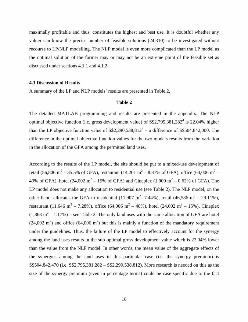
4.3 Discussion of Results

A summary of the LP and NLP models’ results are presented in Table 2.

Table 2

The detailed MATLAB programming and results are presented in the appendix. The NLP

optimal objective function (i.e. gross development value) of S$2,795,381,2824 is 22.04% higher

than the LP objective function value of S$2,290,538,8124 – a difference of S$504,842,000. The

difference in the optimal objective function values for the two models results from the variation

in the allocation of the GFA among the permitted land uses.

According to the results of the LP model, the site should be put to a mixed-use development of

retail (56,806 m2 – 35.5% of GFA), restaurant (14,201 m2 – 8.87% of GFA), office (64,006 m2 –

40% of GFA), hotel (24,002 m2 – 15% of GFA) and Cineplex (1,000 m2 – 0.62% of GFA). The

LP model does not make any allocation to residential use (see Table 2). The NLP model, on the

other hand, allocates the GFA to residential (11,907 m2- 7.44%), retail (46,586 m2 – 29.11%),

restaurant (11,646 m2 – 7.28%), office (64,006 m2 – 40%), hotel (24,002 m2 – 15%), Cineplex

(1,868 m2 – 1.17%) – see Table 2. The only land uses with the same allocation of GFA are hotel

(24,002 m2) and office (64,006 m2) but this is mainly a function of the mandatory requirement

under the guidelines. Thus, the failure of the LP model to effectively account for the synergy

among the land uses results in the sub-optimal gross development value which is 22.04% lower

than the value from the NLP model. In other words, the mean value of the aggregate effects of

the synergies among the land uses in this particular case (i.e. the synergy premium) is

S$504,842,470 (i.e. S$2,795,381,282 – S$2,290,538,812). More research is needed on this as the

size of the synergy premium (even in percentage terms) could be case-specific due to the fact

19

that the possible permutations of permissible land uses and synergies thereof could vary from

case to case.

The optimal solution for each model has 0,0 31 == aa xx (Table 2). This implies that one should

not build residential and office developments right next to retail development(s). This is logical

since residential and office developments located right next to retail development have lower

returns than the same developments located slightly further away. It must be cautioned that this

conclusion is solely based on economic rationality. If it is necessary, for any reason, to build

residential and office units in close proximity to retail units, the requirement can be modelled as

a constraint. All other things being equal, such a constraint will have a negative impact on the

optimal solution. Similarly, the results for the LP and NLP models reveal that it does not make

economic sense to build a retail development adjoining to hotel development given that the latter

would negatively impact such a retail development. Furthermore, the budget constraint

(equation 9) is active in both the NLP and LP model when the unit cost is increased by 3% or

more (column 3-6 of Table 2).

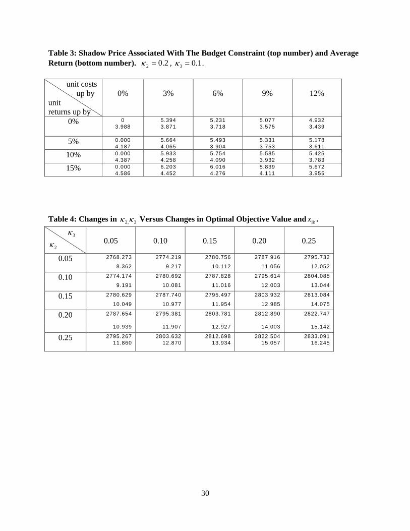
When solving for the optimal solution of a LP/NLP model, one also gets the shadow price

associated with each constraint. The shadow price is zero when the constraint is not active and

positive when the constraint is active. The shadow price iλ associated with the i-th constraint

indicates that if the right-hand side of that constraint is increased by a small amount δ, the

optimal objective function value would increase by the amount δλi . The shadow prices for

various problems associated with the budget constraint (equation 9) are shown in Table 3. Thus

for the problem that corresponds to the second row and third column of Table 3, an increment of

δ units of dollars in the budget would increase the total return by 5.394×δ units of dollars. This is

in contrast to the average return of 3.871 (=2784.238/719.260) units of dollars per unit budget

invested. Thus the analysis suggests that it is desirable to increase the budget where possible.

Table 3

The figures in Table 4 demonstrate the sensitivity of the optimal objective function value to

changes in the positive effects that retail and office developments have on residential property

20

development in the problem. One can see from Table 4 that more residential property will be

built when the positive effects of the retail and office properties on the residential property are

stronger. However, the total net return increases very little (by about 2.3%) from the weakest

effect ( 05.02 =κ , 05.03 =κ ) to the strongest effect ( 25.02 =κ , 25.03 =κ ).

Table 4

It must be noted that the above analysis is based on the assumption that the site is fully

developed to the maximum ratio of building area to lot size as the value of any parcel of land in

Singapore is, among other things, a function of the above ratio. According to Capozza and Li

(1994), a development’s intensity affects construction cost and the optimal decision option.

However, the impact of various design options vis-à-vis the minimum GFA has not been

investigated since the minimum GFA is not a binding constraint at the optimal solution.

5. Valuation of the Site

In consonance with valuation practice in Singapore, the site may be valued via the residual

method by utilizing the figures in the empirical models (equations 7-15) and the summary of the

LP and NLP outputs (Table 2) as presented in Table 5

Table 5

The HBU of the site has been ascertained through the LP model to be retail (56,806 m2), office

(64,006 m2), hotel (24,002 m2), restaurant (14,201 m2), and Cineplex (1,000 m2). Similarly, the

HBU for the site via the NLP model is residential (11,907 m2), retail (46,586 m2), office (64,006

m2), hotel (24,002 m2), restaurant (11,646 m2), and Cineplex (1,868 m2). These optimal

allocations are the bases of the objective function values for both models presented in Table 2.

These objective value figures, together with car parks, form the basis of the total gross

development value from which the site value is derived. Furthermore, the value and construction

costs per m2 of residential, retail and office, restaurant, hotel and Cineplex used for the valuation

(Table 5) are in the empirical model (equations 7-15). All the significant inputs to the residual

valuation model, especially the HBMU, would, at best, be an educated guess without the

LP/NLP modeling of the problem.

21

6. Conclusion

The paper discusses the inability of the Residual method of valuation (and in general all the

traditional methods of valuation including the Cash Flow method) to deal with the optimization

problem involved in the valuation of a mixed-use development site to suggest that a marriage

between management science and the residual methodology provides a more scientifically based,

and therefore, a more supportable estimate of value. It has been argued that the synergism among

the permitted uses on a mixed-use development site makes the assumption of a linear

relationship somewhat simplistic. Thus, the use of the LP model to resolve the optimization

problem involved in the valuation is not intuitively appealing and could lead to inaccurate

valuation. To demonstrate that a NLP modelling is more intuitively appealing, and more

theoretically and empirically sound than the LP model, a real mixed-use development site in

Singapore was modelled via LP and NLP. The results reveal that while the NLP model allocates

the site to all the six permitted uses, the LP model allocates the site to five of the uses excluding

residential use. Furthermore, the NLP model (which accounts for the synergies among the

permitted uses) results in a gross development value that is 22.04% higher than the LP model – a

synergy premium of S$504,842,470. Similarly, the value of the site is 39.81% (S$231,600,000)

higher under the NLP model than the LP model (see Tables 5a&b). This shows that the

assumption of a linear relationship in the valuation of a mixed-use development site could be

problematic.

However, it must be cautioned that the synergy premium, even in percentage terms, could be

peculiar to the case at issue and thus, should not be considered as being of universal application.

It is a function of the permissible land uses and the synergies thereof. Any site with a different

configuration (permissible land uses, synergies, etc.) could result in a different synergy premium.

More research is therefore required on this.

In addition to resolving the optimization problem in an efficient way (in terms of time and cost

savings) to provide a scientifically testable set of significant inputs for the residual valuation

model, the programming results provide sufficient relevant information for objective, elaborate

and persuasive explanation of the optimal solution. Furthermore the models provide relevant

information for monitoring the development of the site as well as for investment counselling.

22

However, the NLP model is both theoretically and intuitively more appealing, more pragmatic

and yields better results than the LP model. Given its ability to resolve the optimization problem

inherent in the HBMU of a mixed-use development site on which valuations are premised vis-à-

vis the availability and advancement in the NLP technology, it is hoped that the valuation

profession and academics, which traditionally gravitate towards finance, will embrace NLP to

improve the quality of the valuation of mixed-use development sites.

23

Endnotes 1 At the time of writing, US$1.00 was equivalent to S$1.365 2 After subtracting the minimum floor areas for retail (5000 m2), office (64,006 m2), hotel (24,002 m2),

if each of the four uses (retail including restaurant, residential, office, hotel) occupies the same amount of

floor space, each use will be allocated 16,752 m2 (i.e. 67,007 m2 ÷ 4). Thus “S$719,259,550” is derived

from 16,752 43

4

12 002,,24006,64000,5 cccc

n

ii +++∑

=

=

3 An oversupply of retail floor area may be modeled by modifying d2a(x) to include a term such as ( )752.16,0max 2 −− axδ to account for the negative effect of oversupplying retail space beyond the

benchmark area of 16.752×1000 m2 under uniform development. Here, δ is a suitable return adjustment to account for the negative impact of oversupply. 4 The magnitude of the gross development value of the newly completed project is very realistic in

Singapore although it may appear preposterous to the western reader.

24

Reference

Addae-Dapaah, K. (2005) Highest and Best use in the Valuation of Mixed-Use Development Sites: A Linear Programming Approach, Journal of Property Research, 22(1), 19-35. Allen, W.C. and Zumwalt, J.K. (1994) Neural Networks: A Word of Caution, Unpublished Working Paper, Colorado State University.

Appraisal Institute (2001) The Appraisal of Real Estate, Appraisal Institute, Chicago.

Avriel, M. (1976) Nonlinear Programming: Analysis and Methods, Prentice Hall, Englewood Cliffs, N.J. Bagnoli, C., Smith, B. and Halbert, C. (1998) The Theory of Fuzzy Logic and its Application to Real Estate Valuation, Journal of Real Estate Research, 16(2), 169-200. Bazaraa, M.S. and Shetty, C.M. (1990) Nonlinear Programming Theory and Algorithms, Wiley & Sons, Singapore. Bertsekas, D.P. (1995) Nonlinear Programming, Athena Scientific, Belmont, Mass. Carter, M.W. and Price, C.C. (2001) Operations Research: A Practical Guide, CRC Press, London.

Capozza, D. and Hesley, R. (1990) The Stochastic City, Journal of Urban Economics, 28, 187-203.

Capozza, D. and Li, Y. (1994) The Intensity & Timing of Investment: The Case of Land, American Economic Review, 84, 889-904.

Dantzig, G.B. and Thapa, M.N. (1997) Linear Programming 1: Introduction, Springer New York.

Do, A.Q. and Grudnitski, G. (1993) A Neural Network Analysis of the Effect of Age on Housing Values, Journal of Real Estate Research, 8(2), 253-64. Everitt, B.S. and Dunn, G. (2001) Applied multivariate data analysis (2nd ed.), Arnold, London. Finch, J.H. (1996) Highest and Best Use and the Special Purpose Property, The Appraisal Journal, 64(2), 195-1999.

25

Gau, G.W., & Kohlhepp, D.B. (1980) The Financial Planning and Management of Real Estate Developments, Financial Management, 9(1), 46-52. Geltner, D., Riddiough, T. and Stojanovic, S. (1996) Insights on the Effect of Land Use Choice: The Perpetual Option on the Best of Two Underlying Assets, Journal of Urban Economics, 39, 20-35.

Goodman, A.C. and Thibodeau, T.G. (1995) Age-Related Heteroskedasticity in Hedonic House Price Equations, Journal of Housing Research, 6, 25-42.

Graaskamp, J.A. (1970) A Guide to Feasibility Analysis, Society of Real Estate Appraisers, Chicago.

Grenadier, S.R. (1995) The Persistence of Real Estate Cycles, Journal of Real Estate Finance and Economic, 10, 95-119.

Grether, D. and Mieszkowski, P. (1974) Determinants of Real Values, Journal of Urban Economics, 1(2), 127-45. Grissom, T.V. (1983) The Semantics Debate: Highest and Best Use Versus Most Probable Use, The Appraisal Journal, 51(1), 45-57.

Hassoun, M.H. (1995) Fundamentals of artificial neural networks, MIT Press, Cambridge, MA. Jain, A.K., Mao, J. and Mohiuddin, K. (1996) Artificial Neural Networks: A Tutorial, Computer, 29(3), 31-44, doi:10.1109/2.485891. Johnson, T., Davies, K, and Shapiro, E. (2000) Modern Methods of Valuation Of Land, Houses and Buildings, Estates Gazette, London.

Kasana, H.S. and Kumar, K.D. (2004) Introductory Operations Research: Theory and Applications, Springer-Verlag, Berlin Heidelberg. Kent, B., Bare, B.B, Field, R.C. and Bradley, G.A. (1991), Natural Resource Land Management Planning Using Large-Scale Linear Programs: The USDA Forest Service Experience with FORPLAN, Operations Research, 39, 13-27. Kuhn, H. and Tucker, A.W. (1951) Nonlinear Programming, in Proceedings of the Second Berkeley Symposium on Mathematical Statistics and Probability (edited by J. Neyman), University of California Press, Berkeley, California, pp. 481-492.

26

Lam, K.C., Yu, C.Y. and Lam, K.Y. (2008) An Artificial Neural Network and Entropy Model for Residential Property Price Forecasting in Hong Kong, Journal of Property Research, 25(4), 321-42. Lennhoff, D.C. and Elhie, W.A. (1995) Highest and Best User, The Appraisal Journal, 63(3), 276-280.

Lee, K.C. and Paik, T.Y. (1996) A Neural Network Approach to Cost Minimization in a Production Scheduling Setting, in Artificial Networks in Real-Life Applications (edited by J.R. Rabunal and J. Dorado), Idea Group Publishing, Hershey PA 17033, pp. 297-313. Liu, J., Zhang, G. X. L., & Wu, W. P. (2006) Application of fuzzy neural network for real estate prediction, LNCS, 3973, 1187–1191. Mehrotra, K., Mohan, C.K., Ranka, S., and Mohan, C.K. (1997) Elements of Artificial Neural Networks, MIT Press, Cambridge, MA. Mehrotra, S. (1992) On the Implementation of a Primal-Dual Interior Point Method, SIAM Journal on Optimization, 2, 575-601.

Mouchly, E., and Peiser, R. (1993) Optimizing Land Use in Multiuse Projects, Real Estate Review, Summer, 23(2), 79-81.

Nguyen, N. and Cripps, A. (2001) Predicting Housing Value: A Comparison of Multiple Regression Analysis and Artificial Neural Networks, Journal of Real Estate Research, 22(3), 313-36. Paxson, D.A. (2005), Multiple State Property Options, Journal of Real Estate Finance and Economics, 30(4), 341-368).

Peiser, R., and Andrus, S.G. (1983), Phasing of Income-Producing Real Estate, Interfaces, 13(5), 1-9.

Peterson, S. and Flanagan, A.B. (2009) Neural Network Hedonic Pricing Models in Mass Real Estate Appraisal, Journal of Real Estate Research, 31(2), 147-64.

Rardin, R.L. (1998) Optimization in Operation Research, Prentice Hall, New Jersey.

Ragsdale, C.T. (2001) Spreadsheet Modeling and Decision Analysis: A Practical Introduction to Management Science, New Jersey:South-Western College Publication, New Jersey.

27

Samuelson, P.A. (1965) Rational Theory of Warrant Pricing, Industrial Management Review, 6, 41-50.

Sarazen, P. (1995) Highest and Best Use of a Vacant Parcel, The Appraisal Journal, 63(3), 281-283.

Sethuraman, J. (2006) Soft Computing Approach for Bond Rating Prediction, in Artificial Networks in Real-Life Applications (edited by J.R. Rabunal and J. Dorado), Idea Group Publishing, Hershey PA 17033, pp. 202-17. Simmons, D.M. (1975) Nonlinear Programming for Operations Research, Prentice Hall, Englewood Cliffs, N.J. Tay, D.P.H. and Ho, D.K.H. (1992) Artificial Intelligence and the Mass Appraisal of Residential Apartments, Journal of Property Valuation and Investment, 10(2), 525-39. Teo Y. (2006) Mixed-Use Developments and Residential Property Values, Department of Real Estate, NUS, Singapore.

Titman, S. (1985) Urban Land Prices Under Uncertainty, American Economic Review, 75, 505-514.

Tsukuda, J. and Baba, S.I. (1994) Predicting Japanese Corporate Bankruptcy in Terms of Financial Data Using Neural Networks, Computers & Industrial engineering, 27(1-4), 445-48.

Wang, L. (1997) A course in fuzzy systems and control, Prentice-Hall, Upper Saddle River, N.J. Williams, T. (1991) Real Estate Development as an Option, Journal of Real Estate Finance and Economics, 4, 209-223.

Wilson, D.C. (1995) Highest and Best Use: Appraisal Heuristics versus Economic Theory, The Appraisal Journal, 63(1), 11-26.

_________ (1996) Highest and Best Use: Preservation Use of Environmentally Significant Real Estate, The Appraisal Journal, 64(1), 76-86. Winokur, H.S., Frick, J.B. and Bean, J.C. (1981) The Affair Between the Land Developer and the Management Scientist, Interfaces, 11(5), 50-56. Worzala, E., Lenk, M. and Silva, A. (1995) An Exploration of Neural Networks and Its Application to Real Estate Valuation, Journal of Real Estate Research, 10(2), 185-201.

28

Table 1: Effects of Synergies among Decision Variables

Decision Variable

ax1 bx1 ax2 bx2 ax3 bx3 4x 5x 6x

ax1 0 0 0.25 0.25 0.05 0.05 0 0 0

bx1 0 0 0.25 0.25 0.05 0.05 0 0 0

ax2 -0.15 0.20 0 0 -0.10 0.20 0 0 0

bx2 -0.15 0.20 0 0 -0.10 0.20 0 0 0

ax3 0.12 0.10 0.07 0.07 0 0 0 0 0

bx3 0.12 0.10 0.07 0.07 0 0 0 0 0

4x 0 0 0 -0.10 to -0.20 0 0 0 0 0

5x 0 0 0 0 0 0 0 0 0

6x 0 0 0.15 to 0.20 0.15 to 0.20 0 0 0 0 0

Note: The figures show the effect that the variables in the “rows” have on the variables in the “columns”.

29

Table 2: Effect of Changes in Unit Costs on Total Optimal Returns. 2.02 =κ , 1.03 =κ . (Objective Function Figures in 1,000,000)

unit costs up by

0%

3%

6%

9%

12%

NLP Optimal Objective Value

2795.381 2784.238 2674.541 2571.085 2473.359

Improvement over LP objective (%)

22.04 21.70 21.06 20.52 19.98

bx1 11.907 10.350 9.335 8.330 7.336

ax2 46.586 46.767 43.973 41.370 38.942

bx3 64.002 64.006 64.006

64.006 64.006

4x 24.002 24.002 24.002

24.002 24.002

5x 11.646 11.692 10.993 10.342 9.735

6x 1.868 3.000 3.000 3.000 3.000

total area 160.016 159.818 155.309 151.051 147.022

budget used 700.934 719.260 719.260 719.260 719.260

LP optimal objective value

2290.539 2287.803 2209.309 2133.372 2061.503

bx1 0 0 0

0 0

ax2 56.806 55.615 51.698 48.263 45.013

bx3 64.006 64.006 64.006

64.006

64.006

4x 24.002 24.002 24.002

24.002 24.002

5x 14.201 13.904 12.925 12.066 11.253

6x 1.000 2.489 3.000 3.000 3.000

total area 160.016 160.016 155.631 151.338 147.275

budget used 700.320 719.260 719.260 719.260 719.260

30

Table 3: Shadow Price Associated With The Budget Constraint (top number) and Average Return (bottom number). 2.02 =κ , 1.03 =κ . unit costs up by unit returns up by

0%

3%

6%

9%

12%

0% 0 3.988

5.394 3.871

5.231 3.718

5.077 3.575

4.932 3.439

5% 0.000 4.187

5.664 4.065

5.493 3.904

5.331 3.753

5.178 3.611

10% 0.000 4.387

5.933 4.258

5.754 4.090

5.585 3.932

5.425 3.783

15% 0.000 4.586

6.203 4.452

6.016 4.276

5.839 4.111

5.672 3.955

Table 4: Changes in 3,2 κκ Versus Changes in Optimal Objective Value and bx1 .

3κ

2κ

0.05

0.10

0.15

0.20

0.25

0.05 2768.273 2774.219 2780.756 2787.916 2795.732

8.362 9.217 10.112 11.056 12.052

0.10 2774.174 2780.692 2787.828 2795.614 2804.085

9.191 10.081 11.016 12.003 13.044

0.15 2780.629 2787.740 2795.497 2803.932 2813.084

10.049 10.977 11.954 12.985 14.075

0.20 2787.654 2795.381

2803.781 2812.890 2822.747

10.939 11.907 12.927 14.003 15.142

0.25

2795.267 11.860

2803.632 12.870

2812.698 13.934

2822.504 15.057

2833.091 16.245

31

Table 5a: Valuation of Site Based on LP Model Value of New Completed Development Objective Function Value S$2,290,538,812 Car parka: 628 lots @ S$800 per lot S$ 502,400 Total - Gross Development Value (GDV) - fval + car park S$2,291,041,212

Deduct Selling expenses (3% of GDV) S$68,731,236 Goods & Services Tax – GST (7% of selling expenses)

S$4,811,187

Goods & Services Tax (7% of GDV) S$160,372,885 Total expenses S$233,915,308 Net Development Value S$2,057,125,904

Deduct: Construction cost including financing cost and professional fees

Retail: 56,806m2 @ S$4,350 per m2 S$247,106,100 Office: 64,006m2 @ S$3,950 per m2 S$252,823,700

Restaurant: 14,201m2 @ S$4,350 per m2 S$61,774,350 Hotel: 24,002m2 @ S$5,650 per m2 S$135,611,300 Cineplex: 1,000m2 @ S$3,000 per m2 S$3,000,000 Car park: 19,500m2 @ S$770 per m2 S$15,015,000 Sub-total S$715,330,450

Add: Developer’s profit (say 20% of GDV) S$458,208,242 Total S$1,173,538,692

Surplus for Land S$883,587,212

Value of Site

Let value of land be x

Add Stamp duty and legal feesb (say 4% of land value) 0.04 x

∴Land value plus stamp duty and legal fees 1.04 x

Add GST (7% of 1.04 x) 0.0728 x

Sub-total 1.1128 x

Add

Cost of finance (say 6% per annum for 5 years) c 0.3763774 x

Property taxd 0.0295195 x

Total Land Cost 1.5186969 x

Thus, 1.5186969 x = S$883,587,212 (i.e. Surplus for land) ∴ x (i.e. value of site) = S$883,587,212/1.5186969 x = S$581,806,165. Thus, the site is valued at say S$581,800,000

a Car parks were not included in the optimization modeling of the problem because they are not included in the

minimum and maximum GFA requirements of the planning guidelines for the “white” site. b Stamp duty and legal expenses related to the purchase of a parcel of land in Singapore account for 2% - 5%

of the value of the land.

32

c Cost of finance is based on the assumption that the development will take 5 years to complete and the cost of

debt is 6% per annum (annual compounding). d Any land under development in Singapore is subject to property tax. The property tax is a function of “annual

value” which, under proviso (f) to s2 of the Property Tax Act (Cap 254, 1985 edition), is 5% of the value of

vacant land. The current property tax rate is 10%. Thus, if the value of the site is X, the “annual value” is

0.05X, and the property tax payable for each year is 0.005X (i.e. 0.05X x 10%). This is payable semi-annually

in advance (i.e. two equal installments of 0.0025X per annum. Therefore, the total amount of property tax

payable over the 5-year holding period and interest accumulation thereof is calculated as:

0.0025 )( ) )( )

+−+×

+×

2/212112 iii n

Although the proceeds of sale are receivable on completion of the

development at a future date, it would be incorrect to discount the proceeds to their present-day value since

“the cost of holding the property is taken as a cost of the development. Therefore to discount the proceeds of

sale would be double counting.” (Johnson et al. 2000:166)

33

Table 5b: Valuation of Site Based on NLP Model Value of New Completed Development Objective Function Value (Exhibit 2) S$2,795,381,282 Car parka: 628 lots @ S$800 per lot S$ 502,400 Total - Gross Development Value (GDV) S$2,795,883,682

Deduct Selling expenses (3% of GDV) S$83,876,510 Goods & Services Tax – GST (7% of selling expenses)

S$5,871,356

Goods & Services Tax (7% of GDV) S$195,711,858 Total expenses S$285,459,724 Net Development Value S$2,510,423,958

Deduct: Construction cost including financing cost and professional fees

Retail: 46,586m2 @ S$4,350 per m2 S$202,649,100 Office: 64,006m2 @ S$3,950 per m2 S$252,823,700

Residential: 11,907m2 @ S$4,500 per m2 S$53,581,500 Restaurant: 11,646m2 @ S$4,350 per m2 S$50,660,100 Hotel: 24,002m2 @ S$5,650 per m2 S$135,611,300 Cineplex: 1,868m2 @ S$3,000 per m2 S$5,604,000 Car park: 19,500m2 @ S$770 per m2 S$15,015,000 Sub-total S$715,944,700

Add: Developer’s profit (say 20% of GDV) S$559,176,736 Total S$1,275,121,436

Surplus for Land S$1,235,302,522

Value of Site

Let value of land be x

Add Stamp duty and legal feesb (say 4% of land value) 0.04 x

∴Land value plus stamp duty and legal fees 1.04 x

Add GST (7% of 1.04 x) 0.0728 x

Sub-total 1.1128 x

Add

Cost of finance (say 6% per annum for 5 years) c 0.3763774 x

Property taxd 0.0295195 x

Total Land Cost 1.5186969 x

Thus, 1.5186969 x = S$1,235,302,522 (i.e. Surplus for land)

∴ x (i.e. value of site) = S$1,235,302,522 /1.5186969

x = S$813,396,355. Thus, the site is valued at say S$813,400,000*

Source: Author • Value of site under NLP model is 39.81% higher than that under LP model

34

Appendix global unit_return D GFA = 160.016; c = [4.500; 4.500; 4.350; 4.350; 3.950; 3.950; 5.650; 4.350; 3.000]; A = [ 1, 1, 1, 1, 1, 1, 1, 1, 1; c(1),c(2),c(3),c(4),c(5),c(6),c(7),c(8),c(9); 0, 0, -1, -1, 0, 0, 0, -1, 0; 0, 0, 0, 0, -1, -1, 0, 0, 0; 0, 0, 0, 0, 0, 0, -1, 0, 0; 0, 0, 0, 0, 0, 0, 0, 0, -1; 0, 0, 0, 0, 0, 0, 0, 0, 1; 0, 0, 0.2, 0.2, 0, 0, 0,-0.8, 0]; b = [GFA; 719.25955; -5.0; -64.0064; -24.0024; -1.000; 3.000; 0.000]; numvar = length(c); LB = 0*ones(numvar,1); UB = inf*ones(numvar,1); unit_return = [12.20; 12.20; 18.840; 18.840; 10.760; 10.760; 13.750; 13.078; 15.850]; kap2 = 0.2; kap3 = 0.1; D = [ 0, 0, -0.15, -0.15, 0.12, 0.12, 0, 0, 0; 0, 0, kap2, kap2, kap3, kap3, 0, 0, 0; 0.25, 0.25, 0, 0, 0.07, 0.07, 0, 0, 0.175; 0.25, 0.25, 0, 0, 0.07, 0.07, -0.15, 0, 0.175; 0.05, 0.05, -0.1, -0.1, 0, 0, 0, 0, 0; 0.05, 0.05, 0.2, 0.2, 0, 0, 0, 0, 0; 0, 0, 0, 0, 0, 0, 0, 0, 0; 0, 0, 0, 0, 0, 0, 0, 0, 0; 0, 0, 0, 0, 0, 0, 0, 0, 0]; %% %% LP model %% options = optimset('Display','off'); [LPsol,LPobj,flag,output,lambda] = linprog(-unit_return,A,b,[],[],LB,UB,[],options); LPsol(3) = LPsol(3)+LPsol(4); LPsol(4)=0;

35

LPsol(6) = LPsol(6)+LPsol(5); LPsol(5)=0; LP.objective = -LPobj; LP.solution = LPsol; LP.dual = lambda.ineqlin; LP.slack = A*LPsol-b; %% %% NLP model %% x0 = LPsol; options = optimset(options,'GradObj','off'); [NLPsol,NLPobj,flag,output,lambda] = fmincon('NLPmodelfun_exp',x0,A,b,[],[],LB,UB,[],options); NLP.objective = -NLPobj; NLP.solution = abs(NLPsol); NLP.dual = lambda.ineqlin; NLP.slack = A*NLPsol-b;