Embed Size (px)
Citation preview

pg 1
Nonlinear, Non-Gaussian Extensions for Ensemble Filter Data Assimilation
Jeff Anderson, AGU, 2019
Jeff Anderson, NCAR Data Assimilation Research Section

pg 2
Bayes’ RuleOutline
Many ensemble assimilation methods are Gaussian & linear.
Tracer applications are neither.
Describe methods to deal with this.

pg 3
−6 −4 −2 0 2 4 60
0.05
0.1
0.15
0.2 Prior PDF
Prob
abilit
y
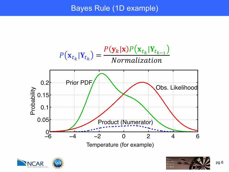
Bayes’ Rule
𝑃 𝐱#$|𝐘#$ =𝑃 𝐲)|𝐱 𝑃 𝐱#$|𝐘#$*+𝑁𝑜𝑟𝑚𝑎𝑙𝑖𝑧𝑎𝑡𝑖𝑜𝑛
Temperature (for example)
Bayes Rule (1D example)
Bayes rule is the key to ensemble data assimilation.

pg 4
−6 −4 −2 0 2 4 60
0.05
0.1
0.15
0.2 Prior PDF
Prob
abilit
y
Bayes’ Rule
𝑃 𝐱#$|𝐘#$ =𝑃 𝐲)|𝐱 𝑃 𝐱#$|𝐘#$*+𝑁𝑜𝑟𝑚𝑎𝑙𝑖𝑧𝑎𝑡𝑖𝑜𝑛
Temperature (for example)
Prior: from model forecast.
Bayes Rule (1D example)

pg 5
−6 −4 −2 0 2 4 60
0.05
0.1
0.15
0.2 Prior PDF
Prob
abilit
y Obs. Likelihood
𝑃 𝐱#$|𝐘#$ =𝑃 𝐲)|𝐱 𝑃 𝐱#$|𝐘#$*+𝑁𝑜𝑟𝑚𝑎𝑙𝑖𝑧𝑎𝑡𝑖𝑜𝑛
Temperature (for example)
Likelihood: from instrument.
Bayes Rule (1D example)
pg 6
−6 −4 −2 0 2 4 60
0.05
0.1
0.15
0.2 Prior PDF
Prob
abilit
y Obs. Likelihood
Product (Numerator)
𝑃 𝐱#$|𝐘#$ =𝑃 𝐲)|𝐱 𝑃 𝐱#$|𝐘#$*+𝑁𝑜𝑟𝑚𝑎𝑙𝑖𝑧𝑎𝑡𝑖𝑜𝑛
Temperature (for example)
Bayes Rule (1D example)

pg 7
−6 −4 −2 0 2 4 60
0.05
0.1
0.15
0.2 Prior PDF
Prob
abilit
y Obs. Likelihood
Normalization (Denom.)
𝑃 𝐱#$|𝐘#$ =𝑃 𝐲)|𝐱 𝑃 𝐱#$|𝐘#$*+𝑁𝑜𝑟𝑚𝑎𝑙𝑖𝑧𝑎𝑡𝑖𝑜𝑛
Temperature (for example)
Bayes Rule (1D example)

pg 8
−6 −4 −2 0 2 4 60
0.05
0.1
0.15
0.2 Prior PDF
Prob
abilit
y Obs. Likelihood
Normalization (Denom.)
Posterior
𝑃 𝐱#$|𝐘#$ =𝑃 𝐲)|𝐱 𝑃 𝐱#$|𝐘#$*+𝑁𝑜𝑟𝑚𝑎𝑙𝑖𝑧𝑎𝑡𝑖𝑜𝑛
Temperature (for example)
Posterior: (analysis).
Bayes Rule (1D example)

pg 9
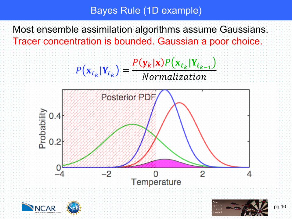
𝑃 𝐱#$|𝐘#$ =𝑃 𝐲)|𝐱 𝑃 𝐱#$|𝐘#$*+𝑁𝑜𝑟𝑚𝑎𝑙𝑖𝑧𝑎𝑡𝑖𝑜𝑛
Bayes Rule (1D example)
Most ensemble assimilation algorithms assume Gaussians.May be okay for quantity like temperature.
pg 10
𝑃 𝐱#$|𝐘#$ =𝑃 𝐲)|𝐱 𝑃 𝐱#$|𝐘#$*+𝑁𝑜𝑟𝑚𝑎𝑙𝑖𝑧𝑎𝑡𝑖𝑜𝑛
Bayes Rule (1D example)
Most ensemble assimilation algorithms assume Gaussians.Tracer concentration is bounded. Gaussian a poor choice.

pg 11
Advection of Tracer -> Nonlinear Prior for Concentration & Wind

pg 12
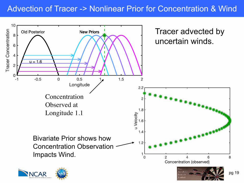
Advection of Tracer -> Nonlinear Prior for Concentration & Wind
Tracer advected by uncertain winds.

pg 13
Advection of Tracer -> Nonlinear Prior for Concentration & Wind
Concentration Observed at Longitude 1.1
Tracer advected by uncertain winds.

pg 14
Advection of Tracer -> Nonlinear Prior for Concentration & Wind
Concentration Observed at Longitude 1.1
Bivariate Prior shows howConcentration ObservationImpacts Wind.
Tracer advected by uncertain winds.

pg 15
Advection of Tracer -> Nonlinear Prior for Concentration & Wind
Concentration Observed at Longitude 1.1
Bivariate Prior shows howConcentration ObservationImpacts Wind.
Tracer advected by uncertain winds.

pg 16
Advection of Tracer -> Nonlinear Prior for Concentration & Wind
Concentration Observed at Longitude 1.1
Bivariate Prior shows howConcentration ObservationImpacts Wind.
Tracer advected by uncertain winds.

pg 17
Advection of Tracer -> Nonlinear Prior for Concentration & Wind
Concentration Observed at Longitude 1.1
Bivariate Prior shows howConcentration ObservationImpacts Wind.
Tracer advected by uncertain winds.

pg 18
Advection of Tracer -> Nonlinear Prior for Concentration & Wind
Concentration Observed at Longitude 1.1
Bivariate Prior shows howConcentration ObservationImpacts Wind.
Tracer advected by uncertain winds.
pg 19
Advection of Tracer -> Nonlinear Prior for Concentration & Wind
Concentration Observed at Longitude 1.1
Bivariate Prior shows howConcentration ObservationImpacts Wind.
Tracer advected by uncertain winds.

pg 20Jeff Anderson, AGU, 2019
Advection of Cosine Tracer: EAKF
Try to exploit nonlinear prior relation between a state variable and an observation.
Example: Observation y~log(x).
Also relevant for variables that are log transformed for boundedness (like concentrations).
MCRHF

pg 21Jeff Anderson, AGU, 2019
Challenges for Tracer Assimilation
Non-Gaussian bounded priors.
Nonlinear bivariate priors.
Solution: More general representation of priors and likelihoods.
Rank Histogram Filters for State Variables.

Marginal Correction Rank Histogram (MCRHF)
−3 −2 −1 0 1 2 3
0
0.2
0.4
0.6
PriorProb
abilit
y D
ensi
ty
Have a prior ensemble for a state variable (like wind).
Marginal Correction Rank Histogram (MCRHF)
−3 −2 −1 0 1 2 3
0
0.2
0.4
0.6
PriorProb
abilit
y D
ensi
ty
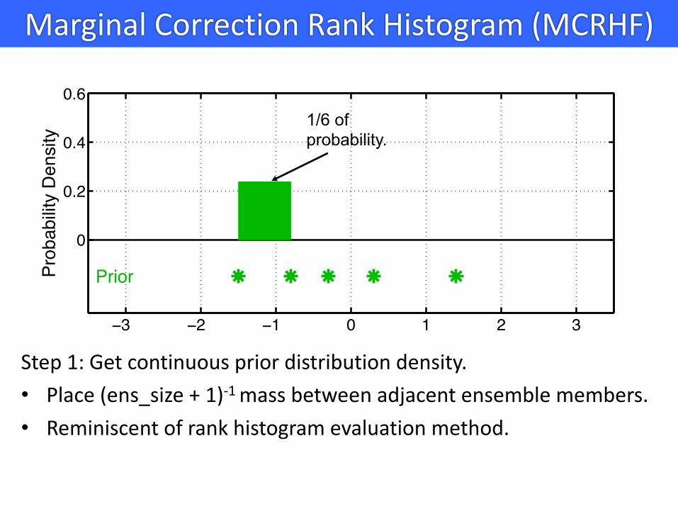
Step 1: Get continuous prior distribution density.• Place (ens_size + 1)-1 mass between adjacent ensemble members.• Reminiscent of rank histogram evaluation method.
1/6 of probability.

Marginal Correction Rank Histogram (MCRHF)
−3 −2 −1 0 1 2 3
0
0.2
0.4
0.6
PriorProb
abilit
y D
ensi
ty
Step 1: Get continuous prior distribution density.• Place (ens_size + 1)-1 mass between adjacent ensemble members.• Reminiscent of rank histogram evaluation method.
1/6 of probability.

Marginal Correction Rank Histogram (MCRHF)
−3 −2 −1 0 1 2 3
0
0.2
0.4
0.6
PriorProb
abilit
y D
ensi
ty
Step 1: Get continuous prior distribution density.• Place (ens_size + 1)-1 mass between adjacent ensemble members.• Reminiscent of rank histogram evaluation method.
1/6 of probability.

Marginal Correction Rank Histogram (MCRHF)
−3 −2 −1 0 1 2 3
0
0.2
0.4
0.6
PriorProb
abilit
y D
ensi
ty
Step 1: Get continuous prior distribution density.• Place (ens_size + 1)-1 mass between adjacent ensemble members.• Reminiscent of rank histogram evaluation method.
1/6 of probability.
Marginal Correction Rank Histogram (MCRHF)
−3 −2 −1 0 1 2 3
0
0.2
0.4
0.6
PriorProb
abilit
y D
ensi
ty
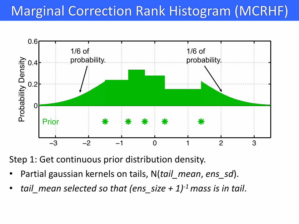
Step 1: Get continuous prior distribution density.• Partial gaussian kernels on tails, N(tail_mean, ens_sd).• tail_mean selected so that (ens_size + 1)-1 mass is in tail.
1/6 of probability.
1/6 of probability.

Marginal Correction Rank Histogram (MCRHF)
Step 2: Get observation likelihood for each ensemble member.

Marginal Correction Rank Histogram (MCRHF)
Step 3: Approximate likelihood with trapezoidal quadrature. • Use long flat tails.

Marginal Correction Rank Histogram (MCRHF)
Step 4: Compute continuous posterior distribution.§ Just Bayes, multiply prior by likelihood and normalize.§ Really simple with uniform likelihood tails.

Marginal Correction Rank Histogram (MCRHF)
Step 5: Compute updated ensemble members:• (ens_size +1)-1 of posterior mass between each ensemble pair.• (ens_size +1)-1 in each tail.

pg 32Jeff Anderson, AGU, 2019
Advection of Cosine Tracer: MCRHF
Try to exploit nonlinear prior relation between a state variable and an observation.
Example: Observation y~log(x).
Also relevant for variables that are log transformed for boundedness (like concentrations).
MCRHF

Details for Marginal Correction RHF method (MCRHF)
Do observation RHF with regression for preliminary posterior.
Get RHF State Marginal.
Rank statistics of posterior same as preliminary posterior.Ensemble member with smallest preliminary posterior value gets smallest posterior value from RHF State Marginal.
Works well for many applications (but more expensive).

pg 34Jeff Anderson, AGU, 2019
MCRHF Capabilities
Ø Enforce additional prior constraints, like boundedness.
Ø Use arbitrary likelihoods.
pg 35Jeff Anderson, AGU, 2019
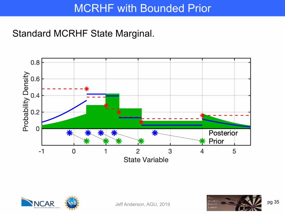
MCRHF with Bounded Prior
Standard MCRHF State Marginal.

pg 36Jeff Anderson, AGU, 2019
MCRHF with Bounded Prior
Bounded State Marginal, same ensemble but positive prior.
1/6 of probability

pg 37Jeff Anderson, AGU, 2019
Bounded State, Non-Gaussian Likelihoods
Bivariate example.
Log of prior is bivariate Gaussian, so prior is non-negative.
One variable observed.
Likelihood is Gamma.Shape parameter is same as first prior ensemble.Scale parameter is 1.
Assimilate single observation for many random priors.

pg 38Jeff Anderson, AGU, 2019
Bounded State, Non-Gaussian Likelihoods
Compare Gamma likelihood to Gaussian approximation.

pg 39Jeff Anderson, AGU, 2019
Bounded State, Non-Gaussian Likelihoods
Compare 3 Methods, 4 Ensemble sizes
Observed Var. Unobserved Var. LikelihoodEAKF Regression GaussianRHF MCRHF GaussianRHF MCRHF Gamma

pg 40Jeff Anderson, AGU, 2019
Percent Negative Posterior Members

pg 41Jeff Anderson, AGU, 2019
Percent Negative Posterior Members
MCRHF both (red and blue) have 0 by design.

pg 42Jeff Anderson, AGU, 2019
RMSE of Posterior Ensemble Mean

pg 43Jeff Anderson, AGU, 2019
RMSE of Posterior Variance

pg 44Jeff Anderson, AGU, 2019
Summary
RHF filters represent non-Gaussian priors, posteriors.
MCRHF allows non-Gaussian, limited non-linearity.
Particularly applicable to bounded quantities like tracers.
MCRHF more expensive, but less than factor of 2.
Ready to test in large applications like tracer transport.Contact me if you’d like to collaborate.

pg 45Jeff Anderson, AGU, 2019
Anderson, J., Hoar, T., Raeder, K., Liu, H., Collins, N., Torn, R., Arellano, A., 2009: The Data Assimilation Research Testbed: A community facility.
BAMS, 90, 1283—1296, doi: 10.1175/2009BAMS2618.1
www.image.ucar.edu/DAReS/DART
All results here with DARTLAB tools freely available in DART.