Nonlinear Optimization: The art of modelingmembers.cbio.mines-paristech.fr/~jvert/teaching/2006insead/slides/... · Nonlinear Optimization: The art of modeling INSEAD, ... Sort out

Nonlinear Optimization:The art of modeling

INSEAD, Spring 2006

Jean-Philippe Vert

Ecole des Mines de Paris

[email protected]

Nonlinear optimization c©2003-2006 Jean-Philippe Vert, ([email protected]) – p.1/34

The art of modeling

Objective: to distill the real-world as accurately andsuccinctly as possible into a quantitative model

Dont want models to be too generalized: might not drawmuch real world value from your results.

Ex: Analyzing traffic flows assuming every person has the

same characteristics.

Dont want models to be too specific: might lose

the ability to solve problems or gain insights.Ex: Trying to analyze traffic flows by modeling every singleindividual using different assumptions.


The four-step rule for modeling

Sort out data and parameters from the verbaldescription

Define the set of decision variables

Formulate the objective function of data and decisionvariables

Set up equality and/or inequality constraints


Problem reformulation

Only few problems can be solved efficiently (LP, QP, ...)

Your problem can often be reformulated in an (almost)equivalent problem that can be solved, up to:

adding/removing variablesadding/removing constraintsmodifying the objective function

Problem reformulation is key for practical optimization!


Model 1: a cheap and healthy diet

A healthy diet contains m different nutrients in quantities atleast equal to b1, . . . , bm. We can compose such a diet withn different food. The j’s food has a cost cj , and contains anamount aij of nutrients i (i = 1, . . . ,m).

How to determine the cheapest healthy diet that satisfies the

nutritional requirements?


A cheap and healthy diet (cont.)

Decision variables: the quantities of the n different food(nonnegative scalars)

Objective function: the cost of the diet, to be minimized.

Constraints: be healthy, i.e., lower bound on thequantities of each food.


A cheap and healthy diet (cont.)

Let x1, . . . , xn the quantities of the n different food. Theproblem can be formulated as the LP:

minimizen

∑

j=1

xjcj

subject ton

∑

j=1

xjaij ≥ bi , i = 1, . . . ,m ,

xj ≥ 0 , j = 1, . . . , n .

This is easily solved (see “Linear Programming” course)


Model 2: Air traffic control

Air plane j, j = 1, . . . , n arrives at the airport within the time

interval [aj , bj ] in the order of 1, 2, . . . , n. The airport wants to

find the arrival time for each air plane such that the narrow-

est metering time (inter-arrival time between two consecu-

tive airplanes) is the greatest.


Air traffic control (cont.)

Decision variables: the arrival times of the planes.

Objective function: the narrowest metering time, to bemaximized.

Constraints: arrive in the good order, and in the goodtime slots.



Let tj be the arrival time of plane j . Then optimizationproblem translates as:

maximize minj=1,...,n−1

(tj+1 − tj)

subject to aj ≤ tj ≤ bj , j = 1, . . . , n ,

tj ≤ tj+1 , j = 1, . . . , n − 1 .

In order to solve it we need to reformulate it in a simpler way.



Reformulation with a slack variable:

maximize ∆


tj ≤ tj+1 , j = 1, . . . , n − 1 ,

∆ ≤ minj=1,...,n−1

(tj+1 − tj) .

Equivalent to the LP (and therefore easily solved):

maximize ∆


tj ≤ tj+1 , j = 1, . . . , n − 1 ,

∆ ≤ tj+1 − tj , j = 1, . . . , n − 1 .


Model 3: Fisher’s exchange market

Buyers have money (wi) to buy goods and maximize their

individual utility functions; Producers sell their goods for

money. The equilibrium price is an assignment of prices to

goods so as when every buyer buys an maximal bundle of

goods then the market clears, meaning that all the money is

spent and all goods are sold.


Fisher’s exchange market


Buyer’s strategies

Let xi,j the amount of good j ∈ G bought by buyer i ∈ B. LetUi(x) = Ui(xi,1, . . . , xi,G) be the utility function of buyer i ∈ B.

Buyer i ∈ B’s optimization problem for given prices pj , j ∈ G

is the following LP :

maximize Ui(x)

subject to∑

j∈G

pjxij ≤ wi ,

xij ≥ 0 , ∀j ∈ G .

Depending on U this is a LP (linear), QP (quadratic), LCCP

(convex)...


Equilibrium price

Without losing generality, assume that the amount of eachgood is 1. The equilibrium price vector p∗ is the one thatensures:

∑

i∈B

x∗(p∗)ij = 1

for all goods j ∈ G, where x∗(p) are the optimal bundle solu-

tions.


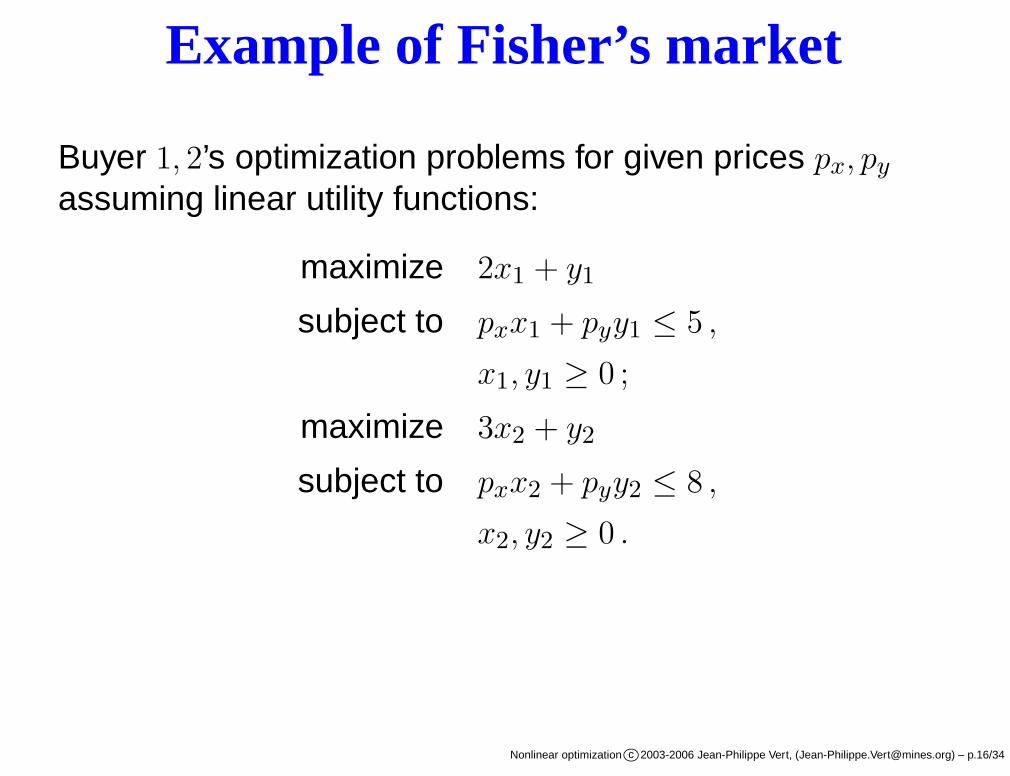
Example of Fisher’s market

Buyer 1, 2’s optimization problems for given prices px, py

assuming linear utility functions:

maximize 2x1 + y1

subject to pxx1 + pyy1 ≤ 5 ,

x1, y1 ≥ 0 ;

maximize 3x2 + y2

subject to pxx2 + pyy2 ≤ 8 ,

x2, y2 ≥ 0 .


Model 4: Chebyshev center

How to find the largest Euclidean ball that lies in apolyhedron described by a set of linear inequalities:

P =(

x ∈ Rn | a>i x ≤ bi, i = 1, . . . ,m

)

.

The center of the optimal ball is called the Chebyshevcenter of the polyhedron; it is the point deepest inside thepolyhedron, i.e., farthest from the boundary.


Chebyshev center (cont.)

The variables are the center xc ∈ Rn and the radius r ≥ 0 of

the ball:B = (xc + u | ‖u ‖2 ≤ r) .

The problem is then

maximize r

subject to B ⊆ P .

We now need to translate the constraint into equations.



For a single half-space defined by the equation a>i x ≤ bi,B

is on the correct halfspace iff it holds that:

‖u ‖2 ≤ r =⇒ a>i (xc + u) ≤ bi .

But the maximum value that a>i u takes when ‖u ‖2 ≤ r isr‖ ai ‖2. Therefore the constraint for a single half-space canbe rewritten as:

a>i xc + r‖ ai ‖2 ≤ bi .



The Chebyshev center is therefore found by solving thefollowing LP:

maximize r

subject to a>i xc + r‖ ai ‖2 ≤ bi , i = 1, . . . ,m .


Model 5: Distance between polyhedra

How to find the distance between two polyhedra P1 and P2

defined by two sets of linear inequalities:

P1 = (x ∈ Rn | A1x ≤ b1) ,

P2 = (x ∈ Rn | A2x ≤ b2) .

x2

x1


Distance between polyhedra (cont.)

The distance between two sets can be written as aminimum:

d(P1,P2) = minx1∈P1,x2∈P2

‖x1 − x2 ‖2 .

The squared distance is therefore the solution of thefollowing QP:

minimize ‖x1 − x2 ‖22

subject to A1x1 ≤ b1 ,

A2x2 ≤ b2 .


Model 6: Portfolio optimization

We consider a classical portfolio problem with n assets orstocks held over a period of time. The vector of relativeprice changes over an investment period p ∈ R

n is assumedto be random variable with known mean p̄ and covarianceΣ. We want to define an investment strategies, whichminimizes the risk (variance) of the return, while ensuringan expected return above a threshold rmin.

This investment strategy has been proposed first by

Markowitz.


Portfolio optimization (cont.)

The decision variable is the portfolio vector x ∈ Rn, i.e., the

amount of each asset xi to buy, in dollars (i = 1 . . . , n). Wecall B the total amount of dollars we can invest.The return in dollars is r = p>x, where p is the vector ofrelative prices changes over the period. The return istherefore a random variable with mean and variance:

E(r) = p̄>x ,

V ar(r) = x>Σx .


Portfolio optimization (cont.)

The Markowitz portfolio optimization problem is thereforethe following QP:

minimize x>Σx

subject to p̄>x ≥ rmin ,

n∑

i=1

xi ≤ B ,

xi ≥ 0 , i = 1, . . . , n .


Model 6: Predicting traffic accidents

We monitor everyday the number of traffic accidents in Paris,

together with several other explanatory variables. The goal

is to make a model to predict the number of accidents from

the explanatory variables, by fitting a Poisson distribution

with mean depending linearly on the explanatory variables

by maximum likelihood on the historical data.


Traffic accidents (cont.)

The Poisson distribution is commonly used to modelnonnegative integer-valued random variables Y (photonarrivals, traffic accidents...). It is defined by:

P (Y = k) =e−µµk

k!,

where µ is the mean.Here we assume that the number of accidents follows aPoisson distribution with a mean µ that depends linearly onthe vector x ∈ R

n of explanatory variables:

µ = a>x + b .

The parameters a ∈ Rn and b ∈ R are called the model

parameters, and must be set according to some principle.Nonlinear optimization c©2003-2006 Jean-Philippe Vert, ([email protected]) – p.27/34


We are given a set of historical data that consists of pairs(xi, yi), i = 1, . . . ,m where yi is the number of trafficaccidents and xi is the vector of explanatory variables atday i. The likelihood of the parameters (a, b) is defined by:

l(a, b) =m∏

i=1

P (yi |xi)

=m∏

i=1

(

a>xi + b)yi

exp(

−(

a>xi + b))

yi!.



Finding the parameter (a, b) by maximum likelihood istherefore obtained by solving the following unconstrainedconvex problem:

maximizem

∑

i=1

{

yi log(

a>xi + b)

−(

a>xi + b)}

.


Model 7: Robust linear discrimination

Given n points in Rp from two classes that can be linearly

separated, find the linear separator that is the furthest awayfrom the closest point.


Robust linear discrimination (cont.)

A linear hyperplane is defined by the equation:

H0 ={

x ∈ Rp : a>x + b = 0

}

,

for some a ∈ Rp and b ∈ R.

Two parallel hyperplanes on ei-ther side are defined by:

H−1 ={

x ∈ Rp : a>x + b = −1

}

,

H1 ={

x ∈ Rp : a>x + b = 1

}

.

w.x+b=0

x2x1

w.x+b > +1

w.x+b < −1w

w.x+b=+1

w.x+b=−1



The distance between H−1 and H1 is equal to 2/‖ a ‖2.Maximizing the distance is equivalent to minimizing‖ a ‖2.

Let yi ∈ {−1,+1} be the label of the point xi. The pointis on the correct region of the space iff:

{

a>xi + b ≥ 1 if yi = 1 ,

a>xi + b ≤ −1 if yi = −1 ,

This is equivalent to:

yi

(

a>xi + b)

≥ 1 .



The optimal separating hyperplane is therefore the solutionof the following QP:

minimize ‖ a ‖2

subject to yi

(

a>xi + b)

≥ 1 , i = 1, . . . , n .

γ

γ


Summary

There are a few general rules to follow to transform areal-world problem into an optimization problem

Most optimization problems are difficult to solve,therefore problem reformulation is often crucial for laterpractical optimization

Problem formulation and reformulation involve a fewclassical tricks (e.g., slack variables) and muchexperience and know-how about which problems canefficiently be solved.


Documents

Nonlinear Optimization: The art of modelingmembers.cbio.mines-paristech.fr/~jvert/teaching/2006insead/slides/... · Nonlinear Optimization: The art of modeling INSEAD, ... Sort out