NONLINEAR PARAMETRIC EXCITATION OF ANEVOLUTIONARY DYNAMICAL SYSTEM

A Dissertation

Presented to the Faculty of the Graduate School

of Cornell University

in Partial Fulfillment of the Requirements for the Degree of

Doctor of Philosophy

by

Rocio Esmeralda Ruelas

January 2015

c© 2015 Rocio Esmeralda Ruelas

ALL RIGHTS RESERVED

NONLINEAR PARAMETRIC EXCITATION OF AN EVOLUTIONARY

DYNAMICAL SYSTEM

Rocio Esmeralda Ruelas, Ph.D.

Cornell University 2015

Evolutionary Dynamics is a field that combines Dynamical Systems with

Game Theory. Game Theory studies the costs and benefits of competing strate-

gies. This competition between strategies is called a “game” and is usually rep-

resented by a payoff matrix. The entries of the payoff matrix represent the loss

or gain received when one type of strategy plays against another. Through the

use of differential equations known as the replicator equations, we can use the

information in the payoff matrix to model the change in relative population (or

frequency) for all of the strategies. Once we have written the evolutionary equa-

tions we can study the dynamics using the methods and theorems developed in

the field of Dynamical Systems.

The Rock-Paper-Scissor model is used to describe systems where there are

three strategies and where each strategy has an advantage over one strategy,

but a disadvantage over the other strategy. The model is named after the classic

game in which Rock beats Scissors, Scissors beats Paper, and Paper beats Rock.

Using the replicator equations, we can model the changes that occur in the rela-

tive populations of the strategies. Strategies whose payoffs are relatively better

will have increasing population frequencies while those with lower payoffs will

have decreasing population frequencies.

In this work, we consider a variation of the standard RPS game where the

payoffs vary periodically in time. In particular, we consider a model with the

following payoff matrix.

R P S

R 0 −1 + A1 cosωt 1 + A2 cosωt

P 1 + A3 cosωt 0 −1 + A4 cosωt

S −1 + A5 cosωt 1 + A6 cosωt 0

(1)

We began our investigation by considering a simple case of our model where

we set A1 = −A2 = A and A3 = A4 = A5 = A6 = 0 thus reducing the number of

parameters down to two. For these parameters we found that, generally, the so-

lutions to the associated replicator equations were quasiperiodic. For some val-

ues of A and ω, solutions that started near the interior equilibrium point would

initially move away from the equilibrium point before eventually returning. Us-

ing a linear perturbation method, we were able to determine the parameter re-

gions for which this behavior occurred. These parameter regions resemble the

tongues of instability characteristic of Mathieu’s equation. We were also able

to determine the effects of nonlinear terms by deriving and analyzing equa-

tions for the slow flow of the replicator equations. We compared those results

to numerically generated Poincare maps and found that they agreed for small

perturbations.

Next we considered a subset of parameters in our proposed payoff matrix

(1) where the interior equilibrium point persists. This results in the following

conditions,

A1 = A6 + A5 − A2 (2)

A3 = A6 + A5 − A4 (3)

We used subharmonic resonance to locate the regions in parameters space

where the interior equilibrium point exhibited linear resonance. We were sur-

prised to discover that for a subset of parameters these regions of linear res-

onance disappeared according to numerical approximations. We then proved

analytically that they did in fact disappear. Finally, we extended our analytical

proof so that it applied to a family of two-dimensional dynamical systems with

time-varying periodic terms.

BIOGRAPHICAL SKETCH

Rocio E. Ruelas was born on September 17, 1986 in Jalisco, Mexico. At the age

of four, she moved with her family to California where she began kindergarten.

Although she did not know any English, Rocio enjoyed school and quickly

caught up to the rest of her classmates. In high school, Rocio excelled in mathe-

matics, but loved learning about the applications in her physics class. Thus, she

decided to pursue a physics major in college.

Rocio attended Harvey Mudd College where she received a B.S. in Physics

in 2008. During her time there, she participated in a number of events concern-

ing diversity in STEM fields and also volunteered as a tour guide. She had the

opportunity to conduct astrophysics research with Professor Ann Esin, but re-

alized through the experience that did not want to become an astrophysicist.

The following summer, she conducted research on network clusters at the Uni-

versity of Michigan - Ann Arbor with Professor Michael Bretz. She very much

enjoyed the mathematical and computational aspects of her research. Hence,

when Rocio applied to graduate schools, she chose programs in Applied Math-

ematics and Mathematical Physics.

After college, Rocio attended the Applied Mathematics program at Cornell

University and received a Cornell Sloan Fellowship for her first three years.

She immediately started working with Professor Richard Rand and managed

to publish five papers during her time there. Rocio continued to participate in

diversity events at Cornell University and volunteered as a Registration Chair

for the Cornell’s Expanding Your Horizons workshop. After her thesis defense,

Rocio plans to teach mathematics courses at Moreno Valley College.

iii

To the Center for Applied Mathematics: Thanks for the memories!

iv

ACKNOWLEDGEMENTS

I have been blessed to be surrounded by a number of people who have sup-

ported me and believed in me throughout my graduate studies. I am forever

grateful to them and hope to one day repay their kindness.

First and foremost, I would like to thank my advisor Richard Rand for his

patience, guidance, and understanding. Aside from teaching me a great deal of

Nonlinear Dynamics, Professor Rand has been an incredible example of what

it means to be a great mentor, researcher, educator, and friend. It is suffice to

say that this thesis would not have been completed without him. I would also

like to thank the members of my committee, Steve Strogatz and Tim Healey, for

their encouragement and direction.

My time in Ithaca might not have been as wonderful without the efforts of

Sara Xayarath Hernandez and the Diversity Programs in Engineering. It was

inspiring as well as incredibly comforting to be surrounded by people passion-

ate about diversity issues. Thank you for all the support, not to mention the free

lunches.

I would like to thank the Alfred P. Sloan foundation and Cornell University

for their financial support in the form of graduate fellowships. I feel very for-

tunate to have had the opportunity to pursue my research without having to

worry about funding.

Finally, I would like to thank my friends and family for keeping me smiling

and grounded. I am especially grateful to my parents for their encouragement

and sacrifice throughout the years.

v

TABLE OF CONTENTS

Biographical Sketch . . . . . . . . . . . . . . . . . . . . . . . . . . . . . . iiiDedication . . . . . . . . . . . . . . . . . . . . . . . . . . . . . . . . . . . ivAcknowledgements . . . . . . . . . . . . . . . . . . . . . . . . . . . . . . vTable of Contents . . . . . . . . . . . . . . . . . . . . . . . . . . . . . . . viList of Figures . . . . . . . . . . . . . . . . . . . . . . . . . . . . . . . . . vii

1 Synopsis 11.1 Motivation . . . . . . . . . . . . . . . . . . . . . . . . . . . . . . . . 11.2 Outline of thesis . . . . . . . . . . . . . . . . . . . . . . . . . . . . . 3

2 Introduction into Evolutionary Games 52.1 Matrix Games and Nash Equilibria . . . . . . . . . . . . . . . . . . 52.2 Evolutionary Stable Strategies . . . . . . . . . . . . . . . . . . . . . 62.3 Replicator Equations . . . . . . . . . . . . . . . . . . . . . . . . . . 8

3 Rock-Paper-Scissor Model 113.1 Dynamics of Standard RPS Model . . . . . . . . . . . . . . . . . . 123.2 Applications of RPS models . . . . . . . . . . . . . . . . . . . . . . 15

4 RPS Model with Periodic Time-Varying Payoffs - A Simple Case 194.1 Model . . . . . . . . . . . . . . . . . . . . . . . . . . . . . . . . . . . 194.2 Simple Case . . . . . . . . . . . . . . . . . . . . . . . . . . . . . . . 204.3 Linear Resonance . . . . . . . . . . . . . . . . . . . . . . . . . . . . 214.4 Multiple Scales Perturbation Method . . . . . . . . . . . . . . . . . 244.5 Poincare map . . . . . . . . . . . . . . . . . . . . . . . . . . . . . . 274.6 Conclusions . . . . . . . . . . . . . . . . . . . . . . . . . . . . . . . 32

5 RPS Model with Periodic Time-Varying Payoffs - The General Case 365.1 Subharmonic Resonance . . . . . . . . . . . . . . . . . . . . . . . . 375.2 Disappearing Tongue . . . . . . . . . . . . . . . . . . . . . . . . . . 425.3 Conclusion . . . . . . . . . . . . . . . . . . . . . . . . . . . . . . . . 46

6 Disapperance of Resonace Tongues 486.1 A Theorem . . . . . . . . . . . . . . . . . . . . . . . . . . . . . . . . 526.2 Application . . . . . . . . . . . . . . . . . . . . . . . . . . . . . . . 556.3 Conclusion . . . . . . . . . . . . . . . . . . . . . . . . . . . . . . . . 56

7 Conclusion 58

Bibliography 60

vi

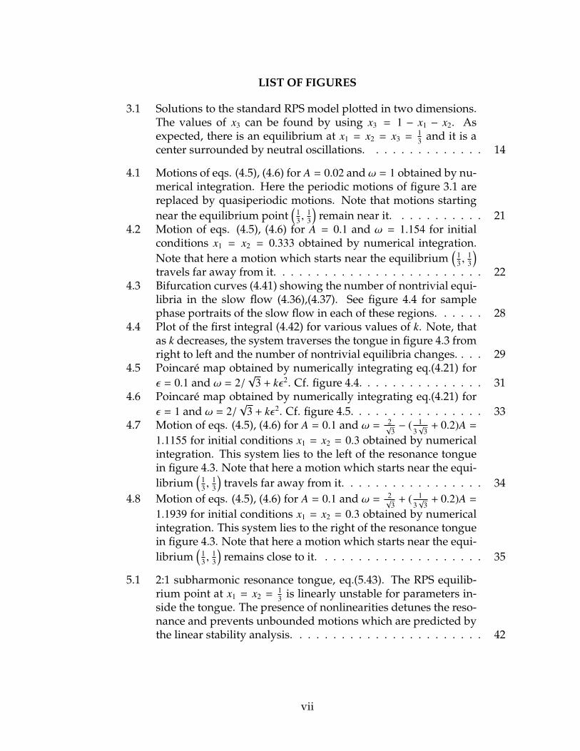
LIST OF FIGURES

3.1 Solutions to the standard RPS model plotted in two dimensions.The values of x3 can be found by using x3 = 1 − x1 − x2. Asexpected, there is an equilibrium at x1 = x2 = x3 =

13 and it is a

center surrounded by neutral oscillations. . . . . . . . . . . . . . 14

4.1 Motions of eqs. (4.5), (4.6) for A = 0.02 and ω = 1 obtained by nu-merical integration. Here the periodic motions of figure 3.1 arereplaced by quasiperiodic motions. Note that motions startingnear the equilibrium point

(13 ,

13

)remain near it. . . . . . . . . . . 21

4.2 Motion of eqs. (4.5), (4.6) for A = 0.1 and ω = 1.154 for initialconditions x1 = x2 = 0.333 obtained by numerical integration.Note that here a motion which starts near the equilibrium

(13 ,

13

)travels far away from it. . . . . . . . . . . . . . . . . . . . . . . . . 22

4.3 Bifurcation curves (4.41) showing the number of nontrivial equi-libria in the slow flow (4.36),(4.37). See figure 4.4 for samplephase portraits of the slow flow in each of these regions. . . . . . 28

4.4 Plot of the first integral (4.42) for various values of k. Note, thatas k decreases, the system traverses the tongue in figure 4.3 fromright to left and the number of nontrivial equilibria changes. . . . 29

4.5 Poincare map obtained by numerically integrating eq.(4.21) forε = 0.1 and ω = 2/

√3 + kε2. Cf. figure 4.4. . . . . . . . . . . . . . . 31

4.6 Poincare map obtained by numerically integrating eq.(4.21) forε = 1 and ω = 2/

√3 + kε2. Cf. figure 4.5. . . . . . . . . . . . . . . . 33

4.7 Motion of eqs. (4.5), (4.6) for A = 0.1 and ω = 2√

3− ( 1

3√

3+ 0.2)A =

1.1155 for initial conditions x1 = x2 = 0.3 obtained by numericalintegration. This system lies to the left of the resonance tonguein figure 4.3. Note that here a motion which starts near the equi-librium

(13 ,

13

)travels far away from it. . . . . . . . . . . . . . . . . 34

4.8 Motion of eqs. (4.5), (4.6) for A = 0.1 and ω = 2√

3+ ( 1

3√

3+ 0.2)A =

1.1939 for initial conditions x1 = x2 = 0.3 obtained by numericalintegration. This system lies to the right of the resonance tonguein figure 4.3. Note that here a motion which starts near the equi-librium

(13 ,

13

)remains close to it. . . . . . . . . . . . . . . . . . . . 35

5.1 2:1 subharmonic resonance tongue, eq.(5.43). The RPS equilib-rium point at x1 = x2 =

13 is linearly unstable for parameters in-

side the tongue. The presence of nonlinearities detunes the reso-nance and prevents unbounded motions which are predicted bythe linear stability analysis. . . . . . . . . . . . . . . . . . . . . . . 42

vii

6.1 The boundaries of the resonance tongue calculated numerically.Red is when µ = 0.5, black is when µ = 0.7, and blue is whenµ = 0.9. The boundaries of the tongue intersect multiple timesand more frequently as µ→ 1. . . . . . . . . . . . . . . . . . . . . 51

viii

CHAPTER 1

SYNOPSIS

The field of Evolutionary Dynamics has grown tremendously since its concep-

tion in the 1940’s and continues to be an exciting area of research. While many

of the principles of evolution have long been accepted as fact in the scientific

community, there still remain a number of unanswered questions regarding the

emergence of certain behaviors or characteristics. The most famous example be-

ing the prominence of cooperation in a variety of species including humans. If

individuals or genes are said to act in their own best interest why then do they

cooperate? Evolutionary Dynamics gives us the tools to address these types of

questions by describing behaviors as strategies and assigning benefits and costs

to each strategy. Furthermore, the population frequency of those strategies can

be described through differential equations where the population frequency of

strategies rise and fall based on their relative fitness. By studying the dynamics

of these differential equations we can determine under what conditions certain

strategies become prevalent in the species. In the case of cooperation, it has been

shown that repeated interactions can lead to the success of a tit-for-tat strategy

which cooperates unless the opposing player has previously defected [2].

1.1 Motivation

In this work, we focus our attention on a specific type of Evolutionary Game

known as Rock-Paper-Scissors (RPS). Like the children’s game with the same

name, the RPS game consists of three strategies where Rock has an advantage

over Scissors which has an advantage over Paper which in turn has an advan-

1

tage over Rock. The version of the RPS game where all strategies have equal

benefits and costs is known as the standard RPS model. The population dy-

namics associated with this model result in cycles where the highest population

frequency alternates between Rock, Paper, and Scissors [6, 7]. In general, all

three strategies will remain in some proportion in the population. This behav-

ior makes the RPS model a useful tool in understanding how biodiversity can

exists in biological or sociological systems.

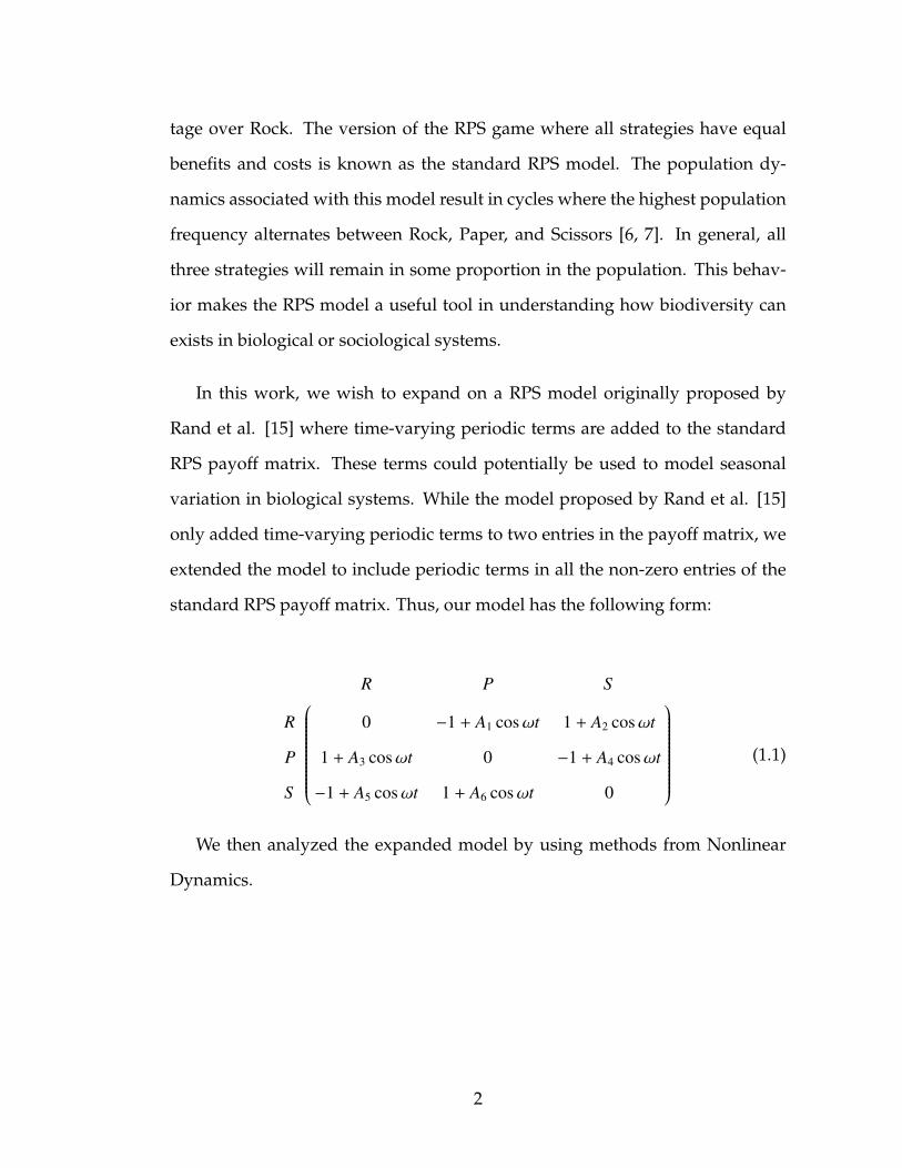
In this work, we wish to expand on a RPS model originally proposed by

Rand et al. [15] where time-varying periodic terms are added to the standard

RPS payoff matrix. These terms could potentially be used to model seasonal

variation in biological systems. While the model proposed by Rand et al. [15]

only added time-varying periodic terms to two entries in the payoff matrix, we

extended the model to include periodic terms in all the non-zero entries of the

standard RPS payoff matrix. Thus, our model has the following form:

R P S

R 0 −1 + A1 cosωt 1 + A2 cosωt

P 1 + A3 cosωt 0 −1 + A4 cosωt

S −1 + A5 cosωt 1 + A6 cosωt 0

(1.1)

We then analyzed the expanded model by using methods from Nonlinear

Dynamics.

2

1.2 Outline of thesis

We begin this work by providing an introduction to evolutionary games in

Chapter 2. A brief history of the field is given and notable terms such as Nash

equilibrium, evolutionary stable strategy, and payoff matrix are defined and ex-

plained. We further describe the use of replicator equations to model population

dynamics of systems with an underlying corresponding payoff matrix.

In Chapter 3 we formally introduce Rock-Paper-Scissor (RPS) models and

discuss the dynamics of the canonical RPS model known as the standard model.

We identify the equilibrium points and general behavior of the standard RPS

model. Applications and prominent papers relating to RPS models are also dis-

cussed.

Chapter 4 introduces the RPS model with time varying coefficients that is

the focus of this work. We consider a simple case with only two parameters

and use perturbation methods to find the regions in parameter space where the

interior equilibrium exhibits linear resonance. Next, we study the system in-

cluding nonlinear terms by using a more powerful perturbation method called

multiple scales. This results in slow flow equations which reveal bifurcation in

the structure of periodic motions in the neighborhood of linear resonance. The

results are then compared with numerically generated Poincare maps for the

full nonlinear system.

Chapter 5 delves further into the time varying RPS model and investigates

the dynamics of the model under the condition that the interior equilibrium

point persists. Using subharmonic resonance, we are able to determine the

boundaries in parameter space that separate the regions of instability of the inte-

3

rior equilibrium from those of stability. These regions are referred to as tongues

of instability. Numerical results suggest that there exists combinations of pa-

rameters for which the tongues of instability disappear. But numerical and per-

turbation results are approximate, whereas the question of whether or not the

tongue disappears is exact. Thus, we proved a theorem to show that the tongues

actually do close up.

In Chapter 6 we generalize the disappearing tongue theorem of Chapter 5 to

apply to a class of linear, periodically forced, dynamical systems.

We conclude our findings in Chapter 7 and discuss the implications of our

results.

4

CHAPTER 2

INTRODUCTION INTO EVOLUTIONARY GAMES

2.1 Matrix Games and Nash Equilibria

In 1944, John von Neumann wrote the groundbreaking text, Theory of Games

and Economic Behavior, in which the field of Game Theory was born [23]. The

book has inspired a mountain of interdisciplinary research, most of which fo-

cuses on two-player matrix games. In two-player matrix games, we imagine

that there is a set of strategies S from which a player may choose. For each

game played we assume that each player chooses a strategy without having

any knowledge of what strategy the opposing player chooses. The choices are

then revealed and the payoffs, i.e. the costs and benefits, are given. All possi-

ble outcomes to the game can be represented in a matrix where the rows of the

matrix correspond to the strategy chosen by the first player and the columns

correspond to the strategy of the second player.

Let us consider a simple example where we only have two strategies (A and B).

The most general form of the payoff matrix would look like,

A B

A a11, b11 a12, b21

B a21, b12 a22, b22

(2.1)

where the values ai j denote the payoff that Player 1 receives when it plays the

strategy in row i and Player 2 plays the strategy in column j. Similarly, bi j is the

payoff that Player 2 receives when it plays the strategy in column i and Player 1

plays the strategy in row j. In this work, we assume that the game is symmetric,

5

meaning that there are no differences between players and ai j = b ji. In this case

the payoff matrix can be simplified to the following,

A B

A a11 a12,

B a21 a22,

(2.2)

One of the major questions that is asked when analyzing games is what strate-

gies will rational players choose. This question lead to the development of one

of the most significant notions in game theory, the Nash equilibrium. Intuitively,

strategies that are Nash equilibria are the best response to themselves. Meaning

that if each player was playing a Nash equilibria, no player can increase their

payoff by switching strategies. More formally, the Nash equilibrium is defined

as,

p · Uq ≤ q · Uq

where U is the payoff matrix, q is the Nash equilibrium, and p is any other

strategy. Thus, p · Uq is the payoff a player receives when playing strategy p

against strategy q. Then q is a Nash equilibrium when no other strategy p does

better against than it does against itself.

2.2 Evolutionary Stable Strategies

While the Nash equilibrium is a very important concept in game theory, it is not

able to explain how certain strategies have become prevalent in a population.

6

This limitation was explored in a paper by Smith and Price titled “The Logic of

Animal Conflict.”[19] Smith and Price sought to understand why animals seem

to end conflicts before either animal is seriously harmed. They devised a two-

player game designed to mimic animal conflict. In a altercation, an animal may

choose to use conventional tactics (C), which are unlikely to to cause serious

injury, or dangerous tactics (D) which are likely to cause serious harm. This

game is now more famously known as the Hawk-Dove game or Cooperation-

Defection game. An example payoff matrix for this type of game would be,

C D

C 2 −2

D 3 −1

(2.3)

From (2.3) we see that if all the animals use conventional tactics they all

benefit, but if just a few use dangerous tactics then those individuals will receive

a higher payoff. Therefore, no matter what the opponent does it is always best

to use dangerous tactics and D is a Nash equilibrium. However, in nature, we

observe that animals tend to use conventional rather than dangerous tactics.

For example, in many snake species the males fight each other by wrestling

without using their fangs [19]. How can the prevalence of conventional tactics

be explained?

Smith and Price were able to explain the rise of conventional tactics by

changing their model to include repeated interactions and mixed strategies. By

including repeated interactions, the animal’s choice can now be informed by the

previous interactions and successful strategies can be adapted by other players.

Also, animals are not limited to only choosing one strategy, but can choose C

7

or D with varying probabilities. Through these changes, Smith and Price were

searching for a strategy that once adopted by a majority of players could not

be be overtaken by variants of that strategy. This is known as an Evolutionary

Stable Strategy or ESS. For understanding how strategies arise and persist in a

population, the ESS is more relevant than a Nash equilibrium.

2.3 Replicator Equations

In order to find and investigate strategies that are evolutionary stable there must

be a dynamical component to the model. The replicator equations are a natural

way to model population dynamics with an underlying payoff matrix.

Replicator dynamics assumes that a population is divided into n groups,

each utilizing different strategies ranging from S i to S n [6].The fraction or fre-

quency that a group appears in the population is denoted by x1, ..., xn. Notice

that since the xi are frequencies then∑

xi = 1. The fitness, fi, of a strategy S i in-

fluences the rate of growth of that population and is determined by the current

state of the population x = {x1, ..., xn} and the payoff matrix. That is, if A is the

associated payoff matrix, and the entry ai j corresponds to the payoff received

by a player playing strategy S i against strategy S j then,

fi(x) =∑

j

ai jx j = (Ax)i (2.4)

We further assume that our population is very large, interactions between

all members of the population happen instantaneously, and the evolution of

the state x(t) is continuous. Based on natural selection, we would expect that

8

strategies who are more fit will have more reproductive success and become a

larger fraction of the population. Therefore, the population dynamics can be

modeled by a system of ordinary differential equations (ODEs), known as the

replicator equations, which have the following form:

xi = xi( fi(x) − f (x)) i = 1, ..., n (2.5)

Here, f (x) is the average fitness of the population frequency.

f (x) =∑

xi fi(x) (2.6)

In eq. (2.5), when a strategy has a fitness above average, the frequency of

that strategy in the population grows. On the other hand, if the fitness is below

average then the frequency of that strategy in the population declines. In this

way, elements of game theory are combined with differential equations to study

the evolution of strategies in a population.

Since we have stipulated that∑

xi = 1, then the dynamics of the replicator

equations lie on the set of non-negative points whose sum is one. This set is

known as the simplex [13]. Essentially, the condition that the population fre-

quencies must sum to one reduces the dimension of the system of replicator

equations by one. For example, if there were two strategies, the simplex would

be a line and if there were three strategies the simplex would be a plane.

The equilibria associated with the replicator equations are connected to the

game theory concepts of Nash equilibriums and evolutionary stable strategies.

Equilibrium points that are asymptotically stable correspond to an evolutionary

stable state, meaning that the population frequencies will not rest at any other

nearby state. Also, equilibrium points in the replicator equations which are

Lyapunov stable correspond to Nash equilibria [6]. Hence, by analyzing the

9

dynamics of the replicator equations for a specific game, we are still able to

draw conclusions of a game theoretic nature.

10

CHAPTER 3

ROCK-PAPER-SCISSOR MODEL

In this work, we wish to consider a game where there are three strategies com-

peting against each other. Each strategy has an advantage over one other strat-

egy, but a disadvantage over the third. This game is most commonly known as

the Rock-Paper-Scissor (RPS) game. There are many games that fall under the

RPS category, but all of them have a payoff matrix that can be reduced to the

following:

R P S

R 0 −a2 b3

P b1 0 −a3

S −a1 b2 0

(3.1)

For now, we assume that ai and bi are positive constants. The replicator equa-

tions for the matrix (3.1) have been well studied [13] and are known to have

three equilibrium points at the vertices of the simplex and one equilibrium in

the interior of the simplex. The stability of the interior equilibrium is depen-

dent on determinant of the payoff matrix. If the determinant of (3.1) is positive,

which corresponds to a1a2a3 < b1b2b3, then the interior equilibrium is globally

stable. If instead the determinant is negative and a1a2a3 > b1b2b3, then the inte-

rior equilibrium is unstable. In the case where a1a2a3 = b1b2b3 the determinant

is zero and the interior equilibrium point is a center surrounded by neutral os-

cillations [13].

We are particularly interested in the dynamics for the case where the deter-

minant of (3.1) is zero. For parameters that satisfy this condition, the replica-

tor equations are structurally unstable, meaning that small perturbations to the

11

equations can lead to qualitatively different dynamics. Therefore, variations of

this RPS model are more interesting to study.

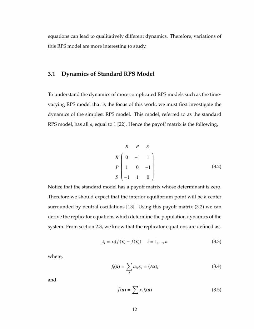
3.1 Dynamics of Standard RPS Model

To understand the dynamics of more complicated RPS models such as the time-

varying RPS model that is the focus of this work, we must first investigate the

dynamics of the simplest RPS model. This model, referred to as the standard

RPS model, has all ai equal to 1 [22]. Hence the payoff matrix is the following,

R P S

R 0 −1 1

P 1 0 −1

S −1 1 0

(3.2)

Notice that the standard model has a payoff matrix whose determinant is zero.

Therefore we should expect that the interior equilibrium point will be a center

surrounded by neutral oscillations [13]. Using this payoff matrix (3.2) we can

derive the replicator equations which determine the population dynamics of the

system. From section 2.3, we know that the replicator equations are defined as,

xi = xi( fi(x) − f (x)) i = 1, ..., n (3.3)

where,

fi(x) =∑

j

ai jx j = (Ax)i (3.4)

and

f (x) =∑

xi fi(x) (3.5)

12

This gives the following fitnesses,

f1 = −x2 + x3 (3.6)

f2 = x1 − x3 (3.7)

f3 = −x1 + x2 (3.8)

which in turn gives an average fitness of zero.

f (x) = x1(−x2 + x3) + x2(x1 − x3) + x3(−x1 + x2) = 0 (3.9)

From eq. 3.3 we see that the replicator equations become

x1 = x1(−x2 + x3) (3.10)

x2 = x2(x1 − x3) (3.11)

x3 = x3(−x1 + x2) (3.12)

and we have a three-dimensional, first-order, nonlinear dynamical system.

Since x1, x2, x3 denote population frequencies, then their sum must equal 1. This

allows us to reduce the dimension of our system down to two by substituting

x3 = 1 − x1 − x2.

x1 = x1(1 − 2x2 − x1) (3.13)

x2 = x2(x2 + 2x1 − 1) (3.14)

Hence the dynamics can be represented on a two dimensional plane. To find

the equilibrium points we set eqs. 3.13-3.14 to zero and solve the system of

equations.

0 = x1(1 − 2x2 − x1) (3.15)

0 = x2(x2 + 2x1 − 1) (3.16)

Doing so gives four equilibrium points. Three points lie at the corners of the

simplex at (0, 0, 1), (0, 1, 0), and (1, 0, 0). The fourth equilibrium is located right

13

at the center of the simplex at(

13 ,

13 ,

13

). A linear stability analysis shows that

the equilibrium points at the corners of the simplex are saddle points, while the

interior equilibrium point is a linear center. Furthermore, eq. 3.13 and eq. 3.14

admit a first integral.

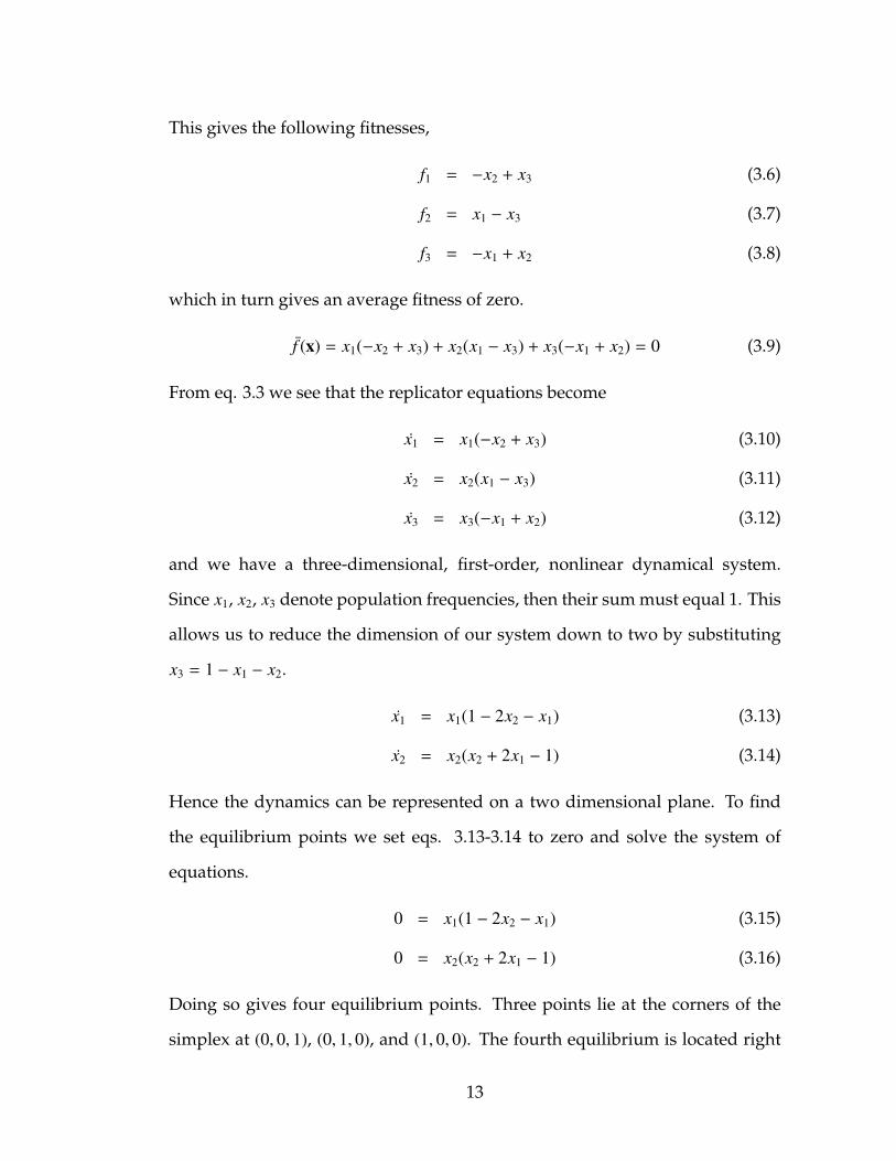
x1x2(1 − x1 − x2) = constant (3.17)

When the integral curves are plotted in figure 3.1, we see that there is indeed

a center at(

13 ,

13 ,

13

)surrounded by neutral cycles. Therefore, in the interior of

simplex and away from the center point, the population frequencies change in

time and no one strategy reaches a stable state.

Figure 3.1: Solutions to the standard RPS model plotted in two dimen-sions. The values of x3 can be found by using x3 = 1 − x1 − x2.As expected, there is an equilibrium at x1 = x2 = x3 =

13 and it is

a center surrounded by neutral oscillations.

14

The standard model is a very special case in the family of RPS models. Any

slight perturbation leads to qualitatively different results. Therefore it is an in-

teresting case to study and a good launching point to investigate more compli-

cated RPS models. The model that is the main focus of this work and introduced

in chapter 4 simplifies to the standard model for certain choices of parameters

and can in fact be considered a perturbation on the standard model for small

values of those parameters.

3.2 Applications of RPS models

RPS models have been used in the biological and social sciences as a means to

understand biodiversity and co-evolution. They apply to systems where there

are three competing strategies or populations and the relationship between the

strategies is similar to the children’s game Rock-Paper-Scissors. Systems that

exhibit this relationship will have population frequencies that periodically os-

cillate.

One example of a biological system that exhibits a rock-paper-scissor dy-

namic is the male population of the side-blotched lizard or Uta stansburiana [18].

Males of the side-blotched lizard have three different colorings on their throats

that correspond to the reproductive strategy they utilize. The males with or-

ange throats have a higher level of testosterone and defend large territories

with a large number of females. Blue-colored males have lower testosterone

and defend smaller territories with less females. The third type is referred to

as a “sneaker” male. It has a yellow-colored throat which resembles the female

side-blotch lizard. Since it appears similar to female side-blotch lizards it is able

15

to sneak into large territories undetected and mate with the females in that terri-

tory. Hence the “sneaker” male had an advantage over the orange-colored male

with the large territory, but not over the blue-colored male with the small terri-

tory since the blue-colored male can more easily defend his territory. However,

the orange-colored male has an advantage over the blue-colored male since he

has access to a larger number of females due to maintaining a larger territory.

Thus, the three reproductive strategies compete in a rock-paper-scissor fashion.

In a paper titled “The rock-paper-scissor game and the evolution of alternative

male strategies,” Sinervo and Lively were able to show that the populations of

the different male types did in fact oscillate with one strategy dominating for a

time before it was overtaken by the strategy that has an advantage over it [18].

Another example of a biological system with a rock-paper-scissor dynamic

is the interaction between three competing strains of Escherichia coli, otherwise

known as E. coli. According to Kirkup and Riley in “Antibiotic-mediated antag-

onism leads to a bacterial game of rock-paper-scissor in vivo,” there exist a strain

of E. coli that produces colicins, which are a type of antibiotic. The antibiotic-

producing strain kills another strain of E. coli that is sensitive to the antibiotic.

However a third strain exists that is resistant to the antibiotic and out competes

the antibiotic strain. When no antibiotic strain is present, the sensitive strain

out competes the resistant strain. Thus these three strains exhibit a rock-paper-

scissor dynamic. In their paper, Kirkup and Riley where able to show that all

three strains of E. coli could coexist as long as their environment were spatially

structured [8].

Rock-paper-scissor dynamics also occur in fields outside of biology. In a

paper by Semmann, Krambeck, and Milinski, the authors give an example

16

of a sociological system with three strategies whose populations oscillate in

a RPS manner [17]. They conducted public goods experiments where people

could anonymously choose from three strategies for an undetermined number

of rounds. Subjects could choose the cooperation strategy which meant that

they joined a group and contributed money to a public pool that is then mul-

tiplied by a factor larger than 1 and distributed evenly amongst members of

the group. Subjects could also choose to join the group and then defect by not

contributing any money. In this way, they receive the benefit of the distributed

money without any of the cost. The third strategy referred to as the “loner”

strategy does not join the group and instead receives a fixed amount money. If

the population is composed of mostly cooperators then the defectors have an

advantage since they receive the group benefit without the cost. However, if the

population consists primarily of defectors then money distributed to the group

will be very low and loners have the advantage. Finally, in a population com-

posed of mostly loners, cooperators can potentially receive more money and

gain an advantage. Similar to the previous papers, the authors found that the

populations of cooperators, defectors, and loners oscillated so that whichever

strategy was most abundant would be overtaken by the strategy which has an

advantage over it.

Due to the number of real-life applications, there are number of papers that

study variations of the RPS model hoping to capture a certain type of behavior

or understand mechanisms for biodiversity. For example, Mauro Mobilia [11]

introduced mutation into the RPS model and found that for low mutation rates

there exists parameters for which the system produces a limit cycle as a result

of a Hopf bifurcation. In this work, we seek to investigate a model that adds

a periodic forcing term to the standard RPS model. One application could be

17

to model the effect of seasonal variation and its impact on the payoffs of the

competing strategies.

18

CHAPTER 4

RPS MODEL WITH PERIODIC TIME-VARYING PAYOFFS - A SIMPLE

CASE

4.1 Model

We are interested in considering a variation of the RPS model that has entries

in the payoff matrix that are time-dependent and periodic. Our motivation is to

create a model that will account for possible seasonal variation in the interac-

tions of the strategies. Previous work done by Rand et al. [15] considers a vari-

ation of the RPS model with two periodic terms added to the standard model.

Our model expands on that work and considers the addition of periodic terms

to all nonzero entries of the payoff matrix. We therefore propose a model of the

following form:

R P S

R 0 −1 + A1 cosωt 1 + A2 cosωt

P 1 + A3 cosωt 0 −1 + A4 cosωt

S −1 + A5 cosωt 1 + A6 cosωt 0

(4.1)

Once we eliminate x3 by applying the constraint x3 = 1 − x1 − x2, the new RSP

model leads to replicator equations of the following type,

x1 = x1(1 − 2x2 − x1) + x1G1(x1, x2; Ai) cosωt (4.2)

x2 = x2(x2 + 2x1 − 1) + x2G2(x1, x2; Ai) cosωt (4.3)

where G1 and G2 are polynomials in x1, x2, and the Ai’s.

The presence of the time-varying periodic terms, Ai cosωt, destroys the first in-

tegral found in the original RPS model. In addition, for general values of Ai, the

equilibrium at(

13 ,

13

)disappears.

19

4.2 Simple Case

We begin our analysis of the proposed model by first studying the model put

forth by Rand et al. [15] If we set A1 = −A2 = −A and A3 = A4 = A5 = A6 = 0 then

our payoff matrix becomes:

R P S

R 0 −1 − A cosωt 1 + A cosωt

P 1 0 −1

S −1 1 0

(4.4)

and the corresponding replicator equations are:

x1 = x1(1 − 2x2 − x1)[1 + (1 − x1)A cosωt] (4.5)

x2 = x2(x2 + 2x1 − 1 + [x1(2x2 + x1 − 1)]A cosωt) (4.6)

This is exactly the model introduced by Rand et al. [15] Numerical integration

shows that for small values of A the periodic motions of the standard RPS sys-

tem are typically replaced by quasiperiodic motions, see figure 4.1. In particular,

motions starting near the equilibrium point(

13 ,

13

)typically remain near it as seen

in figure 4.1. An exception occurs for certain values of the system parameters A

and ω. See figure 4.2 which displays a numerically integrated motion starting

near(

13 ,

13

)for parameters A = 0.1, ω = 1.154. Note that here a motion which

starts near the equilibrium(

13 ,

13

)travels far away from it.

In a previous work done by Rand et al. [15], resonant values of the param-

eters ω and A were identified using Floquet theory and associated instabilities

of the equations linearized about the equilibrium point were studied. Here we

seek to explain the phenomenon in figure 4.1 and figure 4.2 through the use of

perturbation methods. This will allow us to understand non only where such

20

Figure 4.1: Motions of eqs. (4.5), (4.6) for A = 0.02 and ω = 1 obtainedby numerical integration. Here the periodic motions of figure3.1 are replaced by quasiperiodic motions. Note that motionsstarting near the equilibrium point

(13 ,

13

)remain near it.

resonances occur, but also the structure of the phase space in the neighborhood

of parametric resonances.

4.3 Linear Resonance

We begin by translating the origin to the equilibrium at(

13 ,

13

)and scaling the

coordinates by ε << 1. We set

x1 = εx +13, x2 = εy +

13, (4.7)

21

Figure 4.2: Motion of eqs. (4.5), (4.6) for A = 0.1 and ω = 1.154 for initialconditions x1 = x2 = 0.333 obtained by numerical integration.Note that here a motion which starts near the equilibrium

(13 ,

13

)travels far away from it.

and substitute these into eqs.(4.5) and(4.6), giving:

x =(3 εx + 1) ((3 εx − 2 )A cosωt − 3) (2 y + x)

9(4.8)

y =(3 εy + 1)

((6 εx y + 2 y + 3 εx2 + x)A cosωt + 6 x + 3 y

)9

(4.9)

Our first step in the analysis of these ODEs is to determine which values of

ω produce instability via parametric resonance for small values of the forcing

amplitude A. In the work by Rand et al.[15], this was accomplished by using

Floquet theory. Here we obtain this information directly from the perturbation

method as follows. We first linearize (4.8),(4.9) for small values of x and y. This

22

can be done by setting ε = 0, giving:

x = −

(x + 2y

3

)−

29

(2y + x)A cosωt (4.10)

y =(2x + y

3

)+

19

(2y + x)A cosωt (4.11)

Now we look for a solution to these equations via regular perturbations, valid

for small A << 1. The simplest way to do this is to transform this first order

system of ODEs into a single second order ODE by differentiating (4.10) and

substituting expressions for y from (4.11) and for y from (4.10), giving:

f1 x + f2 x + f3x = 0 (4.12)

where

f1 = 3 + 2A cosωt (4.13)

f2 = 2Aω sinωt (4.14)

f3 =

(3 + 2A cosωt

3

)2

(4.15)

We set

x = x0 + A x1 + O(A2) (4.16)

Substituting (4.16) into (4.12) and collecting terms gives:

x0 +x0

3= 0 (4.17)

x1 +x1

3= −

23

x0 cosωt −23ωx0 sinωt −

49

x0 cosωt (4.18)

Eq.(4.17) shows that x0 will have frequency 1/√

3, whereupon the right hand

side of eq.(4.18) will have terms with frequencies:

ω ±1√

3(4.19)

Resonant values of ω will correspond to forcing frequencies (4.19) which are

equal to natural frequencies of the homogeneous x1 equation, i.e. to 1/√

3. This

23

gives that

ω =2√

3(resonance) (4.20)

This value of ω corresponds to the largest resonance tongue. There are an infini-

tude of smaller tongues which would emerge from the perturbation method if

we were to continue it to O(A2) and higher. These have been shown to be of the

form ω = 2/(n√

3) for n = 2, 3, ... [15].

4.4 Multiple Scales Perturbation Method

The resonance (4.20) partially explains the phenomenon displayed in figure 4.2:

when ω lies close to the resonant value of 2√

3, motions which start near the equi-

librium point (x = 0, y = 0) (i.e. (x1 =13 , x2 =

13 )) may move relatively far away

from it. This result is incomplete in that it does not explain how far a motion

will travel from the equilibrium point, how the motion depends on initial con-

ditions, or how close to the resonance value (4.20) the parameter ω must be

chosen for this phenomenon to occur. Here we obtain approximate answers to

these questions by using a more powerful perturbation approach.

We prepare for the perturbation expansion by setting τ = ωt and A = ε2 in

eqs. (4.8), (4.9), and then again transforming the two first order ODEs into a

single second order nonlinear ODE, giving:

18ω2 (3 ε x + 1)(3 ε3 x cos τ − 2 ε2 cos τ − 3

)x′′ =

81 ε ω2(6 ε3 x cos τ − 1

)x′2 − 18 ε2 ω2 sin τ (3 ε x − 2) (3 ε x + 1) x′

− 243 ε9 x6 cos2 τ + 162 ε6 cos τ(2 ε2 cos τ + 3

)x5

24

− 27 ε3(ε4 cos2 τ + 12 ε2 cos τ + 9

)x4 − 18 ε4 cos τ

(5 ε2 cos τ + 9

)x3

+ 3 ε(2 ε2 cos τ + 3

) (2 ε2 cos τ + 9

)x2 + 2

(2 ε2 cos τ + 3

)2x (4.21)

Here primes represent differentiation with respect to τ. Neglecting terms of

O(ε3), we obtain

ω2 x′′ +x3=

ε(3ω2 x′2 − x2

)2

−ε2

(ω2

(81 x x′2 + 12 x′ sin τ

)− 27 x3 + 4 x cos τ

)18

+ O(ε3)(4.22)

Next we define three time scales ξ, η and ζ:

ξ = τ, η = ετ, ζ = ε2τ (4.23)

and we consider x to be a function of ξ, η and ζ, whereupon the chain rule gives:

x′ = xξ + εxη + ε2xζ (4.24)

x′′ = xξξ + 2εxξη + 2ε2xξζ + ε2xηη (4.25)

We detune ω off of the resonance (4.20):

ω =2√

3+ kε2 + · · · (4.26)

and expand x = x0+εx1+ε2x2+· · ·. Substituting (4.24),(4.25) and these expansions

into (4.22) and collecting terms, we obtain:

Lx0 = 0, where L(·) = (·)ξξ +14

(·) (4.27)

Lx1 = −38

x20 − 2x0ξη +

32

x02ξ (4.28)

Lx2 = −34

x0x1 +98

x30 −√

3kx0ξξ −16

x0 cos ξ − 2x1ξη

−2x0ξζ − x0ηη + 3x0ξx1ξ −92

x0x02ξ −

23

x0ξ sin ξ + 3x0ηx0ξ (4.29)

25

We take the solution of (4.27) in the form:

x0 = a0(η, ζ) cosξ

2+ b0(η, ζ) sin

ξ

2(4.30)

Substituting the expression for x0 (4.30) into the x1 equation (4.28), and removing

secular terms gives

∂a0

∂η= 0,

∂b0

∂η= 0 ⇒ a0 = a0(ζ), b0 = b0(ζ) (4.31)

Solving for x1, we obtain

x1 = a1(η, ζ) cosξ

2+ b1(η, ζ) sin

ξ

2+ a0 b0 sin ξ −

12

b02 cos ξ +

12

a02 cos ξ (4.32)

Next we substitute the expression for x1 (4.32) into the x2 equation (4.29), and

remove secular terms, giving

∂a1

∂η= f (a0, b0),

∂b1

∂η= g(a0, b0) (4.33)

where

f (a0, b0) = −da0

dζ+

b0

12−

√3

4kb0 −

34

b30 −

34

a20b0 (4.34)

g(a0, b0) = −db0

dζ+

a0

12+

√3

4ka0 +

34

a30 +

34

b20a0 (4.35)

Now from eq.(4.31) we see that a0 and b0 do not depend on η and thus neither

do f (a0, b0) or g(a0, b0). Eqs.(4.33) show that a1 and b1 will grow linearly in time

η unless f (a0, b0)=0 and g(a0, b0)=0. Thus for a1 and b1 to remain bounded, we

require

da0

dζ=

b0

12−

√3

4kb0 −

34

b30 −

34

a20b0 (4.36)

db0

dζ=

a0

12+

√3

4ka0 +

34

a30 +

34

b20a0 (4.37)

This system of slow-flow equations is easier to study in polar coordinates so we

set a0 = r cos θ and b0 = r sin θ. The slow flow equations become:

∂r∂ζ=

112

r sin 2θ,∂θ

∂ζ=

34

r2 +cos 2θ

12+

√3

4k (4.38)

26

In view of eq.(4.30), equilibrium points in the slow-flow (4.38) correspond to

periodic motions in the standard RPS system (4.5), (4.6). The first of (4.38) gives

θ = 0, π/2, π, 3π/2, whereupon the second of (4.38) gives

34

r2 ±1

12+

√3

4k = 0 ⇒ r2 = ∓

19−

√3

3k (4.39)

Since r2 > 0, we get bifurcations at

k = ±1

3√

3(4.40)

For k > 13√

3there are no nontrivial equilibria, while for k < − 1

3√

3there are four.

In the intermediate case of − 13√

3< k < 1

3√

3there are two nontrivial equilibria.

Since A = ε2 and eq.(4.26), the bifurcation curves have the form:

ω =2√

3±

1

3√

3A + · · · (4.41)

This agrees with the work done by Rand et al. [15] concerning the location of

stability transition curves, see figure 4.3. The slow-flow (4.38) is conservative

and admits the following first integral:

9r4 + 2(3√

3k + cos 2θ)r2 = constant (4.42)

Figure 4.4 displays the first integral (4.42) for k = 13√

3+ 0.2 = 0.3925, k = 0, and

k = − 13√

3− 0.2 = −0.3925, respectively. Here we have identified x with a0, being

approximately x0 at ξ = 0 in eq.(4.30). Similarly, x′ is identified with b0/2.

4.5 Poincare map

The foregoing results of the perturbation method may be compared to numeri-

cal integration of equation (4.21) by use of a Poincare map. Here we imagine a

27

Figure 4.3: Bifurcation curves (4.41) showing the number of nontrivialequilibria in the slow flow (4.36),(4.37). See figure 4.4 for sam-ple phase portraits of the slow flow in each of these regions.

flow on a three-dimensional phase space with axes x,x′,t, and an associated map

produced by sampling the said flow at times τ = 2Nπ, for N = 0, 1, 2, 3, · · ·. The

associated Poincare maps depend upon both ω and ε. Local behavior around

the equilibrium point at the origin x=x′=0 is naturally affected by ω as in figure

4.4. The parameter ε affects both the strength of the forcing (because the forcing

amplitude A = ε2) and the importance of nonlinearities (because the coordinates

have been scaled by ε, cf. eq.(4.7)).

As a check on the perturbation results (which are expected to be valid for

small ε), we first present Poincare maps for ε = 0.1 and for the same values

28

Figure 4.4: Plot of the first integral (4.42) for various values of k. Note,that as k decreases, the system traverses the tongue in figure4.3 from right to left and the number of nontrivial equilibriachanges.

29

of ω as in figure 4.4. See figure 4.5. Note that there is good agreement in the

neighborhood of the origin.

As an example of the kind of behavior which occurs for larger values of ε, we

present Poincare maps for ε = 1 and for the same values of k as in figure 4.5. See

figure 4.6. These figures show the appearance of chaos which is associated with

KAM theory [1]. KAM theory, named for it’s inventors, Kolmogorov, Arnold

and Moser, describes the onset of chaos in a perturbed Hamiltonian system.

Among the various features of KAM theory is the phenomenon that chaos oc-

curs most noticeably in the neighborhood of motions which in the unperturbed

Hamiltonian system are in low order resonance with the periodic driver. This

is relevant to us here because eqs. (4.5), (4.6) may be written in the form of a

perturbed Hamiltonian system:

x1 =∂H∂x2+

A cosωth

∂M∂x2

(4.43)

x2 = −∂H∂x1−

A cosωth

∂M∂x1

(4.44)

where

H = x1x2(1 − x1 − x2) (4.45)

h =−1

x1(1 − x1)2(1 − x1 − 2x2)(4.46)

M =x2

x1 − 1(4.47)

Thus when A=0, the system (4.5), (4.6) is integrable and the Poincare map con-

sists of closed curves as shown in figure 3.1. Then as predicted by KAM theory,

the closed curves in the Poincare map of the unperturbed Hamiltonian system

which are in n : 1 resonance with cosωt are replaced by 2 n−cycles, one stable

and one unstable. The stable n-cycle appears in simulations as n closed curves

30

Figure 4.5: Poincare map obtained by numerically integrating eq.(4.21) forε = 0.1 and ω = 2/

√3 + kε2. Cf. figure 4.4.

31

lying in the neighborhood of the unperturbed resonant curve. The unstable n-

cycle appears as n saddles, each carrying a region of localized chaos with it.

Some of these features may be seen in figure 4.6.

4.6 Conclusions

In this chapter we have investigated a simple case of adding periodic coeffi-

cients to a system which is more commonly treated as having constant coeffi-

cients. The system studied is a replicator equation based on an RPS scenario

characterized by the payoff matrix (4.4) and governed by the differential equa-

tions (4.5), (4.6). In the A=0 constant coefficient case, this system is integrable

with the first integral (3.17) and has the property that the equilibrium at(

13 ,

13

)is

Liapunov stable, figure 3.1. By contrast, in the A>0 system with periodic forcing,

this same equilibrium can be unstable, figure 4.2, due to parametric resonance,

figure 4.3. The analysis presented in this paper, valid for small values of A, has

shown that detuning off of this resonance is, however, asymmetric. That is, sys-

tems which lie outside and just to the left of the resonance tongue of figure 4.3

have very different behavior from those systems which lie just to the right of the

same tongue. See figures 4.7, 4.8. This behavior is predicted by the perturbation

theory, cf. the Poincare maps in figure 4.4. For larger values of A we have seen

that the system studied exhibits KAM type chaos, figure 4.6.

Our results have implications for biological systems with RPS characteristics,

such as the side-blotched lizard Uta stansburiana that displays persistent oscilla-

tions in population frequencies [18]. Previous work has described the dynamics

of this species using an evolutionary model with damping, and has attributed

32

Figure 4.6: Poincare map obtained by numerically integrating eq.(4.21) forε = 1 and ω = 2/

√3 + kε2. Cf. figure 4.5.33

the persistence of the oscillations observed in the data to stochastic perturba-

tions which reset the initial conditions (using a verbal rather than mathematical

argument) [18]. In this work, we have instead approached this issue by consid-

ering an external forcing function that drives the system via periodicity in the

payoff coefficients. We showed how deterministic external forcing can lead to

aperiodic variation in population frequency.

Figure 4.7: Motion of eqs. (4.5), (4.6) for A = 0.1 and ω = 2√

3− ( 1

3√

3+0.2)A =

1.1155 for initial conditions x1 = x2 = 0.3 obtained by numericalintegration. This system lies to the left of the resonance tonguein figure 4.3. Note that here a motion which starts near theequilibrium

(13 ,

13

)travels far away from it.

34

Figure 4.8: Motion of eqs. (4.5), (4.6) for A = 0.1 and ω = 2√

3+ ( 1

3√

3+

0.2)A = 1.1939 for initial conditions x1 = x2 = 0.3 obtainedby numerical integration. This system lies to the right of theresonance tongue in figure 4.3. Note that here a motion whichstarts near the equilibrium

(13 ,

13

)remains close to it.

35

CHAPTER 5

RPS MODEL WITH PERIODIC TIME-VARYING PAYOFFS - THE

GENERAL CASE

We now return to the more general case where our payoff matrix is,

R P S

R 0 −1 + A1 cosωt 1 + A2 cosωt

P 1 + A3 cosωt 0 −1 + A4 cosωt

S −1 + A5 cosωt 1 + A6 cosωt 0

(5.1)

To help with the analysis, we would like to consider values of Ai under which

the equilibrium at(

13 ,

13

)is preserved under periodic forcing. From eqs. (4.2) and

(4.3), this will require that G1 and G2 vanish at x1 = x2 =13 . From that condition,

the following relationship arises between the Ai coefficients:

A1 = A6 + A5 − A2 (5.2)

A3 = A6 + A5 − A4 (5.3)

In the previous chapter we showed that for a specific case where A1 = −A2 = A

and A3 = A4 = A5 = A6 = 0 the interior equilibrium point changed stability for

resonant values of the parameters ω and A. Using perturbation theory, we were

able to detect tongues of instability in the parameter space as well as describe

the nonlinear behavior in the different regions of the tongues. In this chapter,

we seek to investigate the existence of such tongues for the more general case.

36

5.1 Subharmonic Resonance

We begin by investigating the linear stability of the interior equilibrium point.

Recall that the replicator equations for the general model are

x1 = x1(1 − 2x2 − x1) + x1G1 cosωt (5.4)

x2 = x2(x2 + 2x1 − 1) + x2G2 cosωt (5.5)

where

G1 = A2(1 − x1 − x2) + x2[A1 − x1(A1 + A3)] + F (5.6)

G2 = A4(1 − x1 − x2) + x1[A3 − x2(A1 + A3)] + F (5.7)

and

F = (x1 + x2 − 1)[x1(A2 + A5) + x2(A4 + A6)] (5.8)

When we apply the conditions in eqs. (5.2) and (5.3), the governing differential

equations become:

x1 = x1((A6(x22 − x1x2) + A5(x2(1 − x1) + x2

1 − x1) + A4(x22 + x2(2x1 − 1))

+A2(x2(2x1 − 2) + x21 − 2x1 + 1)) cosωt − 2x2 − x1 + 1) (5.9)

x2 = x2((A6(x22 − (x1 + 1)x2 + x1) + A5(x2

1 − x1x2) + A4(x22 + (2x1 − 2)x2 + 1 − 2x1)

+A2(2x1x2 + x21 − x1)) cosωt + x2 + 2x1 − 1) (5.10)

First we move the interior equilibrium point to the origin for convenience.

x1 = x +13, x2 = y +

13

(5.11)

Then substitute eqs. (5.11) into (5.9) and (5.10).

x =19

[cosωt{((9x + 3)y2 + (1 − 9x2)y − 3x2 − x)A6

+((−9x2 + 3x + 2)y + 9x3 − 3x2 − 2x)A5

37

+((9x + 3)y2 + (18x2 + 9x + 1)y + 6x2 + 2x)A4

+((18x2 − 6x − 4)y + 9x3 − 3x2 − 2x)A2}

+y(−18x − 6) − 9x2 − 3x] (5.12)

y =19

[cosωt{(9y3 + (−9x − 3)y2 + (3x − 2y) + 2x)A6

+((−9x − 3)y2 + (9x2−)y + 3x2 + x)A5

+(9y3 + (18x − 3)y2 + (−6x − 2y) − 4x)A4

+((18x + 6)y2 + (9x2 + 9x + 2)y + 3x2 + x)A2}

+9y2 + y(18x + 3) + 6x] (5.13)

For a linear stability analysis, we linearize (5.12) and (5.13).

x =((y − x)A6 + (2y − 2x)A5 + (y + 2x)A4 + (−4y − 2x)A2x) cosωt − 6y − 3x

9(5.14)

y =((2x − 2y)A6 + (x − y)A5 + (−2y − 4x)A4 + (2y + x)A2) cosωt + 3y + 6x

9(5.15)

Now we transform this system of first-order ODEs into a second-order ODE for

convenience in eliminating secular terms in the upcoming perturbation method.

We find

f1 x + f2 x + f3x = 0 (5.16)

where

f1 = −9((A6 + 2A5 + A4 − 4A2) cosωt − 6) (5.17)

f2 = 18(A6 + A5) cosωt − 9ω(A6 + 2A5 + A4 − 4A2) sinωt

−3(A6 + A5)(A6 + 2A5 + A4 − 4A2) cos2 ωt (5.18)

f3 = 18 + 3(A6 − 4A5 − 5A4 + 8A2) cosωt − 9ω(A6 + 2A5 − A4) sinωt

+(−A26 + (−A5 + A4 + 8A2)A6 + 2A2

5 + (11A4 − 8A2)A5 + 2A24 − 16A2A4 + 8A2

2) cos2 ωt

−(A6 + 2A5 + A4 − 4A2)(A2A6 + A4A5 − A2A4) cos3 ωt (5.19)

38

We may now use a perturbation method to determine the stability of the interior

equilibrium, now located at the origin, under the assumption of small forcing

amplitudes. To use the perturbation method we make a change of variables

τ = ωt and denote ′ as a derivative with respect to τ. We also write Ai → εAi. If

we neglect terms of O(ε2), this gives:

g1x′′ + g2x′ + g3x = O(ε2) (5.20)

where

g1 = 54ω2 − 9ω2ε(A6 + 2A5 + A4 − 4A2) cos τ (5.21)

g2 = 18ωε(A6 + A5) cos τ − 9ω2ε(A6 + 2A5 + A4 − 4A2) sin τ (5.22)

g3 = 18 + 3ε(A6 − 4A5 − 5A4 + 8A2) cos τ − 9εω(A6 + 2A5 − A4) sin τ (5.23)

To begin with, we determine the resonant value of ω at O(ε) by setting

x = x0 + εx1 + O(ε2) (5.24)

Substituting (5.24) into (5.20) and collecting terms gives:

x′′0 +x0

3ω2 = 0 (5.25)

x′′1 +x1

3ω2 = H1x′′0 + H2x′0 + H3x0 (5.26)

where

H1 =(A6 + 2 A5 + A4 − 4 A2) cos τ

6(5.27)

H2 =ω(A6 + 2 A5 + A4 − 4 A2) sin τ + (−2 A6 − 2 A5) cos τ

6ω(5.28)

H3 =ω(3 A6 + 6 A5 − 3 A4) sin τ + (−A6 + 4 A5 + 5 A4 − 8 A2) cos τ

18ω2 (5.29)

From (5.25), we see that x0 will have a solution with frequency 1√

3ωwhereupon

the right hand side of eq. (5.26) will have terms with frequencies:

1 ±1√

3ω(5.30)

39

Resonant values of ω will correspond to forcing frequencies (5.30) which are

equal to natural frequencies of the homogeneous x1 equation, i.e. to 1√

3ω. This

gives that

ω =2√

3(resonance) (5.31)

This value of ω corresponds to the largest resonance tongue. There are an infini-

tude of smaller tongues which would emerge from the perturbation method if

we were to continue it to O(ε2) and higher. These have been shown [15] to be of

the form ω0 = 2/(n√

3) for n = 2, 3, ...

In order to investigate the nature of the dynamical behavior in the neighbor-

hood of the resonance (5.31), we define two time scales ξ and η

ξ = τ, η = ετ (5.32)

and we consider x to be a function of ξ and η, whereupon the chain rule gives:

x′ = xξ + εxη (5.33)

x′′ = xξξ + 2εxξη + ε2xηη (5.34)

We detune ω off of the resonance (5.31):

ω =2√

3+ k1ε + · · · (5.35)

and expand x = x0 + εx1 + · · ·. Substituting (5.33), (5.34) and these expansions

into (5.20) and collecting terms, we obtain:

x0ξξ +14

x0 = 0 (5.36)

x1ξξ +14

x1 = −2x0ξη + h1x0ξξ + h2x0ξ + h3x0 +

√3

4k1x0 (5.37)

where the functions hi in eq.(5.37) are the same as the functions Hi in eq.(5.20)

with τ replaced by ξ and ω replaced by 2√

3.

40

We take the solution of (5.36) in the form:

x0 = a(η) cosξ

2+ b(η) sin

ξ

2(5.38)

We substitute the expression for x0 (5.38) into the x1 equation (5.37), and remove

secular terms, giving the slow flow:

∂a∂η= a

(A4 − A5

8√

3

)+ b

− √34

k1 +A2 − A6

12+

A4 − A5

24

(5.39)

∂b∂η= −b

(A4 − A5

8√

3

)+ a

√34

k1 +A2 − A6

12+

A4 − A5

24

(5.40)

Eqs. (5.39), (5.40) are a constant coefficient linear system with the following

eigenvalues:

±1

12

√−27k2

1 + (A2 − A6)2 + (A4 − A5)2 + (A2 − A6)(A4 − A5) (5.41)

For given parameters A2, A4, A5, A6, the equilibrium point a = b = 0 will be ei-

ther unstable (exponential growth) or stable (quasiperiodic motion) depending

respectively on whether the eigenvalues (5.41) are real or imaginary. The transi-

tion between stable and unstable will correspond to zero eigenvalues, given by

the condition:

27k21 = (A2 − A6)2 + (A4 − A5)2 + (A2 − A6)(A4 − A5) (5.42)

Eq. (5.42) will yield two values of k1, let’s call them k1 = ±Q, which from eq.

(5.35) plot as two straight lines in the ω − ε plane, representing the boundaries

of the 2:1 subharmonic resonance tongue, see figure 5.1. Inside this tongue the

equilibrium is unstable due to parametric resonance:

ω =2√

3± Qε, Q =

√(A2 − A6)2 + (A4 − A5)2 + (A2 − A6)(A4 − A5)

√27

(5.43)

41

Figure 5.1: 2:1 subharmonic resonance tongue, eq.(5.43). The RPS equilib-rium point at x1 = x2 =

13 is linearly unstable for parameters in-

side the tongue. The presence of nonlinearities detunes the res-onance and prevents unbounded motions which are predictedby the linear stability analysis.

5.2 Disappearing Tongue

In the special case that A2 = A6 and A4 = A5, we see from eq. (5.43) that Q = 0

and the tongue has closed up, at least to O(ε). For these parameter values we

have from eqs. (5.2), (5.3):

A1 = A4 = A5 ≡ αε, A2 = A3 = A6 ≡ βε (5.44)

42

so that the payoff matrix (4.1) becomes:

R P S

R 0 −1 + αε cosωt 1 + βε cosωt

P 1 + βε cosωt 0 −1 + αε cosωt

S −1 + αε cosωt 1 + βε cosωt 0

(5.45)

where ω = 2/√

3, and the linearized differential eqs. (5.14), (5.15) become:

x =(yαε − (x + y)βε) cosωt − 2y − x

3(5.46)

y =(−(x + y)αε + xβε) cosωt + y + 2x

3(5.47)

From Floquet theory [20],[15] we know that on the transition curves which de-

fine the two sides of the tongue, i.e. which separate regions of stability from

regions of instability, there exists a periodic solution having frequency ω/2 (a

“subharmonic”). To prove that the tongue has truly disappeared (rather than

approximately so as in perturbation theory), we must show that there COEXIST

two linearly independent solutions having frequency ω/2. To make this easier

to consider, define a new subharmonic time scale T = (ω/2)t = t/√

3. Then eqs.

(5.46), (5.47) become:

1√

3

dxdT

=(yαε − (x + y)βε) cos 2T − 2y − x

3(5.48)

1√

3

dydT

=(−(x + y)αε + xβε) cos 2T + y + 2x

3(5.49)

Here we must show that there exists two linearly independent solutions with

frequency 1 in T . For example, when α=β=0, there are two linearly independent

solutions with frequency 1:

x =√

3 cos T − sin T, y = 2 sin T (5.50)

and

43

x = −2 sin T, y =√

3 cos T + sin T (5.51)

That is, we are forcing the system at twice its natural frequency. The idea here is

that there normally exists a solution of frequency 1 on each transition curve. In

order to show that there is no tongue, we have to show that the two transition

curves are coincident. In fact we claim that the two transition curves correspond

to k1 = Q = 0, that is, to a single vertical line in the ω−ε plane, going through the

point ω = 2/√

3, ε = 0. Eqs. (5.48), (5.49) correspond to such a vertical line, and

so we want to show that there are two linearly independent solutions to these

equations.

Numerical simulations of eqs. (5.48), (5.49) have shown that this result is valid

to all orders of ε, i.e., eqs. (5.48), (5.49) exhibit a frequency 1 solution for all

nontrivial initial conditions, regardless of the values of α, β or ε. That is, the

tongue really does close up and the instability disappears. Moreover, numerical

evidence shows that all the other tongues in the ε − ω plane (which emanate

from points on the ω-axis at ω = 2/(n√

3), see [15]) also close up and disappear.

We supplement these numerical results with the following

THEOREM: All nontrivial solutions to eqs. (5.48), (5.49) are periodic with fre-

quency 1.

Proof: We assume a solution to eqs. (5.46), (5.47) in the form (“variation of

parameters”):

x = u(√

3 cos T − sin T ) + v(−2 sin T ) (5.52)

44

y = u(2 sin T ) + v(√

3 cos T + sin T ) (5.53)

where u and v are functions of T to be found. Note that (u = 1, v = 0) gives (5.50),

while (u = 0, v = 1) gives (5.51). Substituting (5.52), (5.53) into (5.48), (5.49) gives

the following eqs. on u and v:

√3

dudT

= ε cos 2T (−βu + (α − β)v) (5.54)√

3dvdT

= ε cos 2T ((β − α)u − αv) (5.55)

Next we define new time variable z:

dz =ε cos 2T√

3dT ⇒ z =

ε sin 2T

2√

3(5.56)

which gives the following constant coefficient linear system on u,v:

ddz

u

v

= −β α − β

β − α −α

u

v

(5.57)

The matrix in (5.57) has eigenvalues:

λ = −(α + β

2

)± i

√3

2(β − α) (5.58)

Thus the general solution to (5.57) involves a linear combination of terms of the

form

exp(α + β

2z) sin

cos

√

32

(β − α)z (5.59)

Therefore since z is a π-periodic function of T , we see that u and v also have pe-

riod π in time T . Then from (5.52), (5.53), it follows that x and y have period 2π

in T , since the product of a π-periodic function and a 2π-periodic function has

period 2π. Q.E.D.

45

5.3 Conclusion

From a dynamical systems point of view, we may summarize our findings as

follows: The original RPS system, with payoff matrix (3.2) and no forcing, ex-

hibits an equilibrium at(

13 ,

13

)which is stable. With the addition of forcing,

there will generally be a 2:1 subharmonic resonance region in parameter space

in which the equilibrium becomes unstable. In this chapter we have shown that

this tongue may be absent or very small if the forcing parameters are chosen

appropriately.

In the case that the equilibrium is linearly unstable, the presence of nonlin-

earities detunes the resonance (because the frequency of the motion changes as

the amplitude increases) and prevents the unbounded motions which are pre-

dicted by the linear stability analysis. The resulting unstable motion is either

quasiperiodic or chaotic as described in Chapter 4.

From a biological and social point of view, the presence of periodic forcing

in RPS can lead to quasiperiodic or chaotic oscillations, such as those observed

in the range of biological and social applications. Seemingly stochastic fluctua-

tions in strategy frequencies need not necessarily arise from a stochastic process,

as we have shown in earlier work in the previous chapter. Now we see that de-

pending on the choice of forcing parameters, it is possible to reduce or even

eliminate quasiperiodic motion. Thus, if one was designing an organization,

community or political system where stability was desired, this effect could be

achieved by properly tuning the degree of periodic forcing. A similar logic ap-

plies to biological systems. If the forcing coefficients were themselves subject

to natural selection, evolution might favor coefficients that eliminate the tongue

46

and result in stable population frequencies.

47

CHAPTER 6

DISAPPERANCE OF RESONACE TONGUES

In the previous chapter, we were able to show that for certain parameters the

largest resonance tongue at ω = 2√

3completely disappears and there coexists

two linearly independent solutions that are both 2π periodic. In this chapter

we consider a more general system of ODEs for which the previous system,eqs.

(5.48), (5.49), is a subset of. Here we aim to prove that the resonance tongues

disappear in the general system given certain parameters and that the system in

the previous chapters meets those conditions. We begin by providing a motivat-

ing example that captures the result we obtained in our previous chapter. Here

we use perturbation methods to find approximate solutions which will sug-

gest that for some special parameters there is no region of instability. However,

since these are only approximate solutions we cannot be certain the tongue has

indeed disappeared. The system with periodic coefficients that we encountered

in eqs. (5.48) and (5.49) can be written in the form:

√3 δ

dxdt= (−1 + 2(µ − 1)ε cos 2t)x + (−2 + (2 + µ)ε cos 2t)y (6.1)

√3 δ

dydt= (2 + (1 − 4µ)ε cos 2t)x + (1 − (1 + 2µ)ε cos 2t)y (6.2)

where δ, µ and ε are parameters. For fixed µ, we picture the δ−ε plane and desire

to know for which regions all solutions to (6.1) and (6.2) are bounded (in which

case these equations are said to be stable, and for which regions unbounded

solutions exist (unstable). We are interested in the limit in which ε → 0 so we

expand δ = 1 + kε + O(ε2). As in the case of Mathieu’s equation [14] [20], there

is, for typical values of µ, a tongue of instability emanating from the point δ = 1,

ε = 0 on the δ-axis. This instability is caused by a 2:1 subharmonic resonance.

48

This can be seen by noting that for ε=0, eqs. (6.1) and (6.2) take the form

√3

ddt

x

y

= −1 −2

2 1

x

y

(6.3)

Eqs. (6.3) have the general solution: x

y

= A

√

3 cos t − sin t

2 sin t

+ B

−2 sin t√

3 cos t + sin t

(6.4)

where A and B are arbitrary constants. Note that the forcing function in eqs.

(6.1) and (6.2), cos 2t, has twice the frequency of the solution (6.4) of the unforced

system (6.3), which is the source of the 2:1 resonance. We seek an approximate

solution to eqs.(6.1) and (6.2) valid for small ε by using the two variable expan-

sion method [14], also known as the method of multiple scales [12]. We replace

the independent variable t by two time variables, ξ = t and η = εt, whereupon

eqs. (6.1) and (6.2) become:

√3 (1 + kε + O(ε2))

(∂x∂ξ+ ε

∂x∂η

)= (−1 + 2(µ − 1)ε cos 2ξ)x + (−2 + (2 + µ)ε cos 2ξ)y(6.5)

√3 (1 + kε + O(ε2))

(∂y∂ξ+ ε

∂y∂η

)= (2 + (1 − 4µ)ε cos 2ξ)x + (1 − (1 + 2µ)ε cos 2ξ)y(6.6)

Next we expand x = x0 + εx1 +O(ε2) and y = y0 + εy1 +O(ε2) and collect terms,

giving:

√3∂x0

∂ξ= −x0 − 2y0 (6.7)

√3∂y0

∂ξ= 2x0 + y0 (6.8)

√3∂x1

∂ξ= −x1 − 2y1 + 2(µ − 1)x0 cos 2ξ + (2 + µ)y0 cos 2ξ −

√3k∂x0

∂ξ−√

3∂x0

∂η(6.9)

√3∂y1

∂ξ= 2x1 + y1 + (1 − 4µ)x0 cos 2ξ − (1 + 2µ)y0 cos 2ξ −

√3k∂y0

∂ξ−√

3∂y0

∂η(6.10)

49

Eqs. (6.7), (6.8) have the solution (cf. eqs. (6.4)): x0

y0

= A(η)

√

3 cos ξ − sin ξ

2 sin ξ

+ B(η)

−2 sin ξ√

3 cos ξ + sin ξ

(6.11)

Next we substitute eqs. (6.11) into eqs. (6.9), (6.10) and trigonometrically reduce

the resulting equations, which are of the form:

√3∂x1

∂ξ= −x1 − 2y1 + M1 cos ξ + M2 sin ξ + N.R.T. (6.12)

√3∂y1

∂ξ= 2x1 + y1 + M3 cos ξ + M4 sin ξ + N.R.T. (6.13)

where N.R.T. stands for Non-Resonant Terms, and where the coefficients Mi are

known functions of A(η) and B(η), omitted here for brevity. For no secular terms

in x1 and y1, the following relationships must hold:

2M1 + M3 +√

3M4 = 0 (6.14)

2M2 −√

3M3 + M4 = 0 (6.15)

Eqs. (6.14), (6.15) give the following slow flow:

2√

3dAdη

= (2k + µ − 1)A + (4k − µ + 1)B (6.16)

2√

3dBdη

= (4k + 2µ − 2)A + (2k + µ − 1)B (6.17)

Eqs. (6.16), (6.17) are a linear constant coefficient system with eigenvalues

λ = ±12

√(µ − 1)2 − 4k2 (6.18)

The transition between stable and unstable corresponds to λ=0:

λ = 0⇒ k = ±12

(µ − 1) (6.19)

Since δ = 1+kε+O(ε2), we see that the tongue of instability has boundaries given

by:

δ = 1 ±12

(µ − 1)ε + O(ε2) (6.20)

50

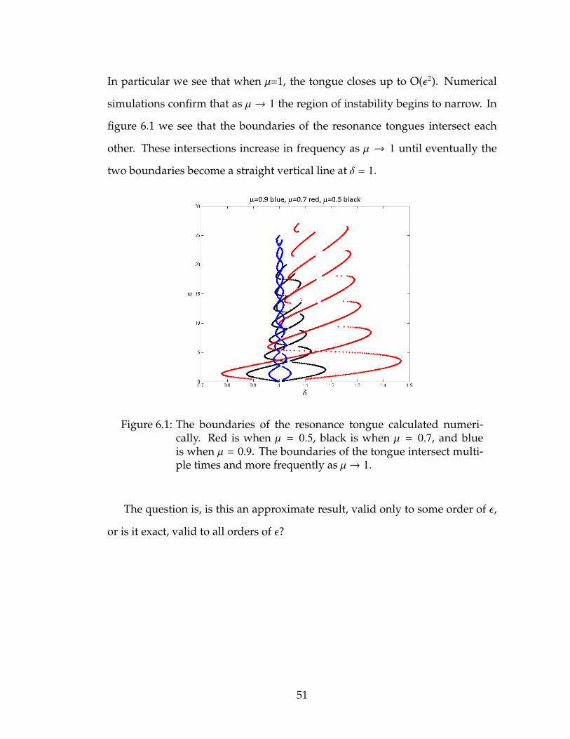
In particular we see that when µ=1, the tongue closes up to O(ε2). Numerical

simulations confirm that as µ → 1 the region of instability begins to narrow. In

figure 6.1 we see that the boundaries of the resonance tongues intersect each

other. These intersections increase in frequency as µ → 1 until eventually the

two boundaries become a straight vertical line at δ = 1.

Figure 6.1: The boundaries of the resonance tongue calculated numeri-cally. Red is when µ = 0.5, black is when µ = 0.7, and blueis when µ = 0.9. The boundaries of the tongue intersect multi-ple times and more frequently as µ→ 1.

The question is, is this an approximate result, valid only to some order of ε,

or is it exact, valid to all orders of ε?

51

6.1 A Theorem

In this section we generalize the preceding example by considering a system in

the following form:

dxdt= a1(t) x + a2(t) y (6.21)

dydt= a3(t) x + a4(t) y (6.22)

where

ai(t) = Pi + ε Qi cos 2t (6.23)

We assume that when ε=0, the system (6.21), (6.22) has a pair of linearly inde-

pendent solutions of period 2π (cf. eqs. (6.4)), which we write in the form:

x = A F1(t) + B F2(t) (6.24)

y = A G1(t) + B G2(t) (6.25)

where A and B are arbitrary constants.

The goal is then to find conditions on the coefficients Pi and Qi such that

eqs. (6.21), (6.22) have two linearly independent solutions of period 2π for all

ε >0.The coexistence of these two solutions for all ε >0 means that the associ-

ated 2:1 resonance tongue has closed up, both boundaries being coincident. (As

we saw in the foregoing example, in general each boundary of the tongue pos-

sesses a period 2π solution. If the system (6.21), (6.22) possesses two linearly

independent period 2π solutions, then both tongue boundaries are coincident,

and the tongue has closed up.)

52

When ε=0, eqs.(6.21),(6.22) become

ddt

x

y

= P1 P2

P3 P4

x

y

(6.26)

For eqs.(6.26) to exhibit two linearly independent solutions of period 2π, its

eigenvalues must be ±i. This requires that the trace of the matrix in (6.26) be

zero, and its determinant be unity, giving:

P4 = −P1 (6.27)

P3 =−1 − P2

1

P2(6.28)

Then without loss of generality we may take the two linearly independent pe-

riod 2π solutions in (6.24), (6.25) to be:

F1(t) = sin t, G1(t) = ν1 sin t + ν2 cos t (6.29)

and

G2(t) = sin t, F2(t) = ν3 sin t + ν4 cos t (6.30)

where the νi coefficients may be found by substituting (6.29), (6.30) into the ε=0

equations (6.26), giving:

ν1 = −P1

P2(6.31)

ν2 =1P2

(6.32)

ν3 = −P1P2

1 + P21

(6.33)

ν4 = −P2

1 + P21

(6.34)

Having characterized the solution of eqs.(6.21), (6.22) for ε=0, we now go after

the solution for ε >0.

53

We posit a solution for ε >0 using variation of parameters (cf.

eqs.(6.24),(6.25)):

x = u(t) F1(t) + v(t) F2(t) (6.35)

y = u(t) G1(t) + v(t) G2(t) (6.36)

where u(t) and v(t) are unknown functions to be found. Substituting (6.35), (6.36)

into (6.21), (6.22), and solving for du/dt and dv/dt, we get

dudt= ε cos 2t

[H1 sin2 t + H2 sin t cos t + H3

](6.37)

dvdt= ε cos 2t

[H4 sin2 t + H5 sin t cos t + H6

](6.38)

where Hi = Hi(P1, P2,Qi, u, v) are known functions, too long to list here.

Motivated by a desire to find conditions which guarantee a pair of linearly

independent solutions to eqs. (6.21), (6.22), we set H1 = H2 = H4 = H5 = 0, which

requires

Q2 = −P2

2P1(Q4 − Q1) (6.39)

Q3 =(1 + P2

1)2P1P2

(Q4 − Q1) (6.40)

Assuming that conditions (6.39), (6.40) are fulfilled, eqs.(6.37),(6.38) become:

dudt= ε cos 2t

[Q4 u −

P2

2P1(Q4 − Q1) v

](6.41)

dvdt= ε cos 2t

[1 + P2

1

2P1P2(Q4 − Q1) u + Q1 v

](6.42)

Next we reparameterize t by using a new time scale τ defined as:

τ =12

sin 2t (6.43)

54

which transforms (6.41), (6.42) into a system with constant coefficients:

dudτ= ε

[Q4 u −

P2

2P1(Q4 − Q1) v

](6.44)

dvdτ= ε

[1 + P2

1

2P1P2(Q4 − Q1) u + Q1 v

](6.45)

Although the solution of eqs. (6.44), (6.45) depends on the numerical values

of the coefficients P1, P2, Q1, Q4, it will in general consist of sinusoidal and or

exponential functions of τ, and since τ is π-periodic in t by eq.(6.43), u(t) and v(t),

the solution functions of (6.44), (6.45), will be π-periodic in t. Furthermore, we

note by eqs. (6.35), (6.36), that x(t) and y(t), the solution functions of eqs. (6.21),

(6.22), are composed of terms which are the product of π-periodic functions (i.e.

u(t) and v(t)) and 2π-periodic functions (i.e. Fi(t) and Gi(t)). Now since the prod-

uct of a π-periodic function and a 2π-periodic function has period 2π, we see

that all solutions of eqs. (6.21), (6.22) are 2π periodic.

We have therefore proved the following

THEOREM: All nontrivial solutions of eqs. (6.21), (6.22) will have period 2π

if eqs. (6.27), (6.28), (6.39), (6.40) are satisfied.

6.2 Application

In this section we apply the theorem of the previous section to the example

presented earlier in this chapter. Eqs. (6.1), (6.2), when expressed in the form of

55

eqs. (6.21), (6.22) yield the following values for the coefficients Pi and Qi:

P1 = −1√

3(6.46)

P2 = −2√

3(6.47)

P3 =2√

3(6.48)

P4 =1√

3(6.49)

Q1 =−2 + 2µ√

3(6.50)

Q2 =2 + µ√

3(6.51)

Q3 =1 − 4µ√

3(6.52)

Q4 = −1 + 2µ√

3(6.53)

Inspection shows that these values for Pi and Qi satisfy eqs .(6.27), (6.28), (6.39),

(6.40) in the case that µ=1. Therefore we may conclude by the foregoing theorem

that the closing of the tongue at µ=1 is an exact result and is valid to all orders

of ε.

6.3 Conclusion

The perturbation methods used to find approximate solutions to eqs. (6.1), (6.2)

suggest that for the special value of µ = 1 there exists no region of instability.

Meaning that the resonance tongue has disappeared. The results, however, are

only approximate and using this method we cannot account for all of the higher

order terms. Therefore we set out to prove the disappearance of the resonance

tongue in a different manner. We consider a more general class of differential

equations, seen in eqs. (6.21)-(6.25), for which our original problem is an exam-

56

ple of. We chose our parameters carefully so that solutions are guaranteed to

be comprised of two bounded and linearly independent functions of period 2π.

This leads to the choice of parameters found in eqs. (6.27), (6.28), (6.39), (6.40).

We then show that our original problem satisfies those conditions and, hence,

does not exhibit a resonance tongue.

57

CHAPTER 7

CONCLUSION

We began our investigation of the RPS model with time-varying coefficients

by considering a simple case where there were only two parameters, A and ω.

While the standard RPS model is characterized by neutral cycles surrounding

the interior equilibrium point, our model showed quasiperiodic behavior and

evidence of a change in stability in the interior equilibrium point. We then

sought to find for which values of A and ω the interior equilibrium point ex-

hibited linear resonance. Through perturbation analysis we found that there

existed tongues of instability in the parameter space and that inside of these

tongues the interior equilibrium point was unstable. Using a multiple-scale

perturbation method we were able to derive equations for the slow flow of the

system and see the difference in behavior of the model both inside and outside

of the resonant tongue. We found the the tongue was not symmetric, meaning

the behavior to the left of the tongue was qualitatively different then the behav-

ior to the right of the tongue. The results from the slow flow are valid for small

values of A and are supported by numerically generated Poincare maps. For

large values of A we see the appearance of chaos which is associated with KAM

theory.

Following the case with only two parameters, we investigated the dynamics

of our time-varying RPS model for all parameter values for which the interior

equilibrium point remained. We found that, in general, our model has a 2:1

subharmonic resonance region in parameter space where the interior equilib-

rium becomes unstable. Using multiple time scales and perturbation methods

we were able to determine to linear order the boundaries in parameter space for

58

the instability region. We were surprised to find that there existed values for Ai

in which our linear approximation of the boundary would disappear. Numeri-

cal integration tests also showed that the instability region had closed. In order

to show that the instability region had indeed disappeared and was not sim-

ply too small to find numerically we sought to prove the result analytically. To

prove that the resonant tongue had disappeared for those parameter values we

needed to show that there coexisted two linearly independent solutions having

frequency ω/2. Using variation of parameters, we were able to postulate a form

of the solution to a scaled version of our dynamical system. We proved that the

solution we postulated did in fact solve our differential equations and that it

was composed of two linearly independent terms having frequency ω/2.

Next we expanded our proof of disappearing tongues of instability to apply

to a broader set of differential equations of which our previous system belonged.

Again, using variation of parameters we were able to find conditions on our

proposed solutions for which there existed two linearly independent solutions

that were 2π periodic.

59

BIBLIOGRAPHY

[1] V.I. Arnold and A. Avez. Ergodic Problems of Classical Mechanics. Benjamin,New York, 1968.

[2] Robert M. Axelrod. The Evolution of Cooperation. Basic books, 2006.

[3] Carl M. Bender and Steven A. Orszag. Advance Mathematical Methods for Sci-entists and Engineers: Asymptotic Methods and Perturbation Theory. Springer,1999.

[4] Ross Cressman. Evolutionary Dynamics and Extensive Form Games. The MITPress, 2003.

[5] John Guckenheimer and Philip Holmes. Nonlinear Oscillations, DynamicalSystems, and Bifurcations of Vector Fields. Springer, New York, 1983.

[6] Josef Hofbauer and Karl Signmund. Evolutionary Games and Population Dy-namics. Cambridge University Press, 1998.

[7] Benjamin Kerr, Margaret A. Riley, Marcus W. Feldman, and Brendan J. M.Bohannan. Local dispersal promotes biodiversity in a real-life game ofrock-paper-scissors. Nature, 2002.

[8] Benjamin C. Kirkup and Margaret A. Riley. Antibiotic-mediated antago-nism leads to a bacterial game of rock-paper-scissors in vivo. Nature, 2004.

[9] Yuri A. Kuznetsov. Elements of Applied Bifurcation Theory. Springer, NewYork, 2004.

[10] W. Magnus and S. Winkler. Hill’s Equation. Interscience Publishers (Wiley),New York, 1966.

[11] Mauro Mobilia. Oscillatory dynamics in rock-paper-scissor games withmutations. Journal of Theoretical Biology, 2010.

[12] A. H Nayfeh and D. T. Mook. Nonlinear Oscillations. Wiley, NY, 1979.

[13] Martin A. Nowak. Evolutionary Dynamics: Exploring the Equations of Life.The Belknap Press of Harvard University Press, 2006.

60

[14] Richard H. Rand. Lecture notes on nonlinear vibrations (version 53), May2012.

[15] Richard H. Rand, Max Yazhbin, and David G. Rand. Evolutionary dy-namics of a system with periodic coefficients. Communications in NonlinearScience and Numerical Simulation, 2011.

[16] Geoff Recktenwald and Richard H. Rand. Coexistence phenomenon inautoparametric excitation of two degree freedom systems. International J.Nonlinear Mechanics, 2005.

[17] Dirk Semmann, Hans-Jurgen Krambeck, and Manfred Milinski. Volunteer-ing leads to rock-paper-scissors dynamics in a public goods game. Nature,2003.

[18] B. Sinervo and C. M. Livelyi. The rock-paper-scissors game and the evolu-tion of alternative male strategies. Nature, 1996.

[19] J. Maynard Smith and G.R. Price. The logic of animal conflict. Nature, 1973.

[20] James J. Stoker. Nonlinear Vibration in Mechanical and Electrical Systems. Wi-ley, NY, 1950.

[21] Steven H. Strogatz. Nonlinear Dynamics and Chaos: With Applications toPhysics, Biology, Chemistry, and Engineering. Westview Press, Cambridge,MA, 1994.

[22] T.L. Vincent and J.S. Brown. Evolutionary Game Theory, Natural Selection, andDarwinian Dynamics. Cambridge University Press, 2005.

[23] John von Neumann and Oskar Morgenstern. Theory of Games and EconomicBehavior. Princeton University Press, 1944.

61