-. .. c . . N 7 1 - 2 7 7 8 5

V A R I A N T S O F T H E S E C A N T M E T H O D F O R S O L V I N G N O N L I N E A R S Y S T E M S OF E Q U A T I O N S

C l a r e n c e C a n t o r

G o d d a r d S p a c e F l i g h t Center G r e e n b e l t , M a r y l a n d

J a n u a r y 1 9 7 1

NATIONAL TECHNICAL INFORMATION SERVICE

* e m - e*-e eee-e e e. em- ee*

- 0 e.. *e e .

e*.

I-::.m e

0. -e

_. -mee.e

L O A N COPY: RETURN TO AFWL (DOGL)

KlRTLAND AFB, N. M.

Dislributed ...' to foster, serve and promote the nation's

economic development and technological

advancement.'

U.S. DEPARTMENT O F COMMERCE

- _ _ This document has been approved for public release and sale.

- I

https://ntrs.nasa.gov/search.jsp?R=19710018309 2018-08-18T19:40:24+00:00Z

-

i VARIANTS OF THE SECANT METHOD FOR SOLVING NONLINEAR

,

SYSTEMS OF E Q U A T I O N S

, ' \

CLARENCE CANTOR

Y

JANUARY 1971

-GODDARD SPACE FLIGHT CEN.TER ' . I

. J

Reproduced by . NATIONAL TECHNICAL

INFORMATION SERVICE Springfield, Va. 22151

I

, ,

.-. .- . . . .. ... . I -

~ . .. ..-

X-733-71-48

VARIANTS OF THE SECANT METHOD FOR SOLVING

NONLINEAR SYSTEMS OF EQUATIONS

Clarence C antor

January 1971

GODDARD SPACE FLIGHT CENTER Greenbelt, Maryland

VARIANTS OF THE SECANT METHOD FOR SOLVING

NONLINEAR SYSTEMS OF EQUATIONS

Clarence Cantor

ABSTRACT

Some variants of the Secant Method a re developed for solving f (x) = 0,

n nonlinear equations in n unknowns. The new methods, consisting of

Algorithms I and 11, depart from existing versions of the Secant Method

whenever certain conditions arise that would tend to cause poor con­

vergence of the latter. These conditions are ascertained via simple

test criteria associated with the new algorithms. When these criteria

a re satisfied initially at each step, the algorithms follow the same steps

as existing versions of the Secant Method and, under certain assump­

tions, a r e shown to possess superlinear convergence. Whenever these

test criteria are not satisfied initially, the algorithms follow logical

alternate procedures that provide a basis for linear convergence. The

results of numerical experiments with a series of randomly generated

problems support the claim of improved convergence for the new

methods. Of the two new algorithms, Algorithm I1 is judged to be the

superior and w a r r a n t s further numerical investigation.

iii

PRECEDING PAGE E m CONTENTS

Section

ACKNOWLEDGEME NTS ...........................................

INTRODUCTION ..................................................

I. BACKGROUND ...............................................

11. ALGORITHMS I AND 11. ...................................... 2.1 Introduction .............................................. 2.2 Algorithm I .............................................. 2.3 Algorithm 11 .............................................

Page-vii

ix

1-1

2-1

2-1

2-2

2-12

111. LOCAL CONVERGENCE OF ALGORITHMS I AND II.. . ......... 3-1

I V . NUMERICAL EXPERIMENTS.. ................................ 4-1

V . CONCLUSIONS ............................................... 5-1

REFERENCES.................................................... R-1

APPENDIX 1. ALTERNATE ORTHOGONAL1ZATION PROCEDURE FOR ALGORITHMS IB AND IIB..................... Al-1

APPENDIX 2. PROGRAMMING ................................... A2-1

V

c

LIST OF TABLES

Table Page

4-1 Convergence of n = 2 Problems............................. 4-9

4-2 Convergence of n = 5 Problems ............................ 4-10

4-3 Convergence of n = 10 Problems ............................ 4-11

4-4 Convergence of n = 15 Problems ........................... 4-12

4-5 Comparative Performance of Group 1 Algorithms ............ 4-16

4-6 Comparative Performance of Group 2 Algorithms ............ 4-17

vi

ACKNOWLEDGEMENTS

The author wishes to thank Dr. F. P. Emad of the University of

Maryland for his guidance during this research. The research

was supported by the Goddard Space Center of the National

Aeronautics and Space Administration.

vii

VARIANTS OF THE SECANT METHOD FOR SOLVING

NONLINEAR SYSTEMS OF EQUATIONS

INTRODUCTION

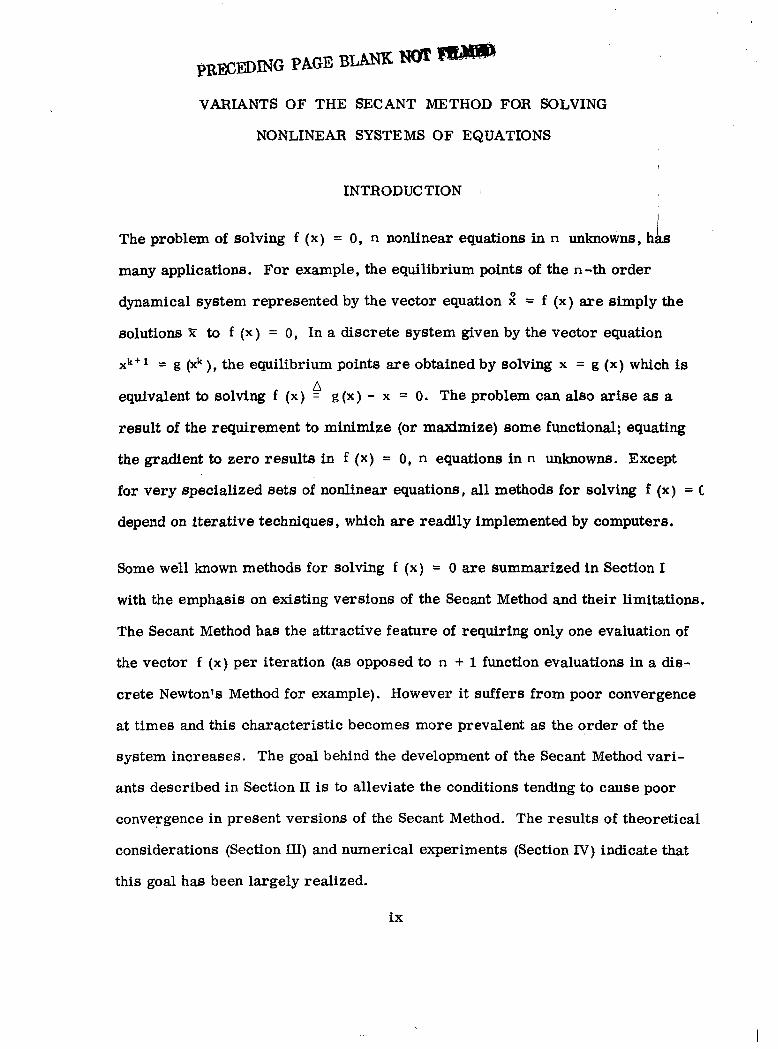
The problem of solving f (x) = 0, n nonlinear equations in n unknowns, hIs many applications. For example, the equilibrium points of the n-th order

dynamical system represented by the vector equation = f (x)are simply the

solutions a to f (x) = 0, In a discrete system given by the vector equation

xkt = g (xk), the equilibrium points are obtained by solving x = g (x) which is n

equivalent to solving f (x) = g ( x ) - x = 0. The problem can also arise as a

result of the requirement to minimize (or maximize) some functional; equating

the gradient to zero results in f (x) = 0, n equations in n unknowns. Except

for very specialized sets of nonlinear equations, all methods for solving f (x) = C

depend on iterative techniques, which a r e readily implemented by computers.

Some well known methods for solving f (x) = 0 are summarized in Section I

with the emphasis on existing versions of the Secant Method and their limitations.

The Secant Method has the attractive feature of requiring only one evaluation of

the vector f (x)per iteration (as opposed to n + 1function evaluations in a dis­

crete Newton's Method for example). However it suffers from poor convergence

at times and this characteristic becomes more prevalent as the order of the

system increases. The goal behind the development of the Secant Method vari­

ants described in Section I1 is to alleviate the conditions tending to cause poor

convergence in present versions of the Secant Method. The results of theoretical

considerations (Section III) and numerical experiments (Section N)indicate that

this goal has been largely realized.

ix

SECTION I

BACKGROUND

nL.+wton's Method in n dimensions (see e.g., [ 111 [16], 171, and [23])is

probably the most widely known method for solving the n-th order vector equa­

tion f (x) = 0. Analogous to the case of one dimension, Newton's Method in n

\. \dimensions is given by $9 U. I -"b,­

1 /* P Xk+l = xk - J'%(xk) f (xk) (1.1)

(assuming J' (xk) exists)

where

f (xk)is the value of f (x) at x = x k

J (xk)is the Jacobian matrix of f (x) evaluated at xk

xk is the present (k -th) estimate of the n -dimensional solution I

and

xk+' is the next estimate of the solution.

Newton's Method is a direct result of linearizing the system f (x) = 0 about the

point x = xk. A Taylor's expansion of f (x) about x = xk , in which all terms

above the first order a r e dropped, yields (1.1).

Assuming f (x ) is continuously differentiable in a neighborhood of a solution X

and that the Jacobian matrix is nonsingular in this neighborhood, Newton's

Method wi l l converge to F if the starting estimate x1 is "sufficiently close" to

R . In practice, Newton's Method suffers from three principal disadvantages:

1. The region of convergence in some problems may be very small. Thus the

method may fail to converge for all but fairly accurate initial estimates x l .

1-1

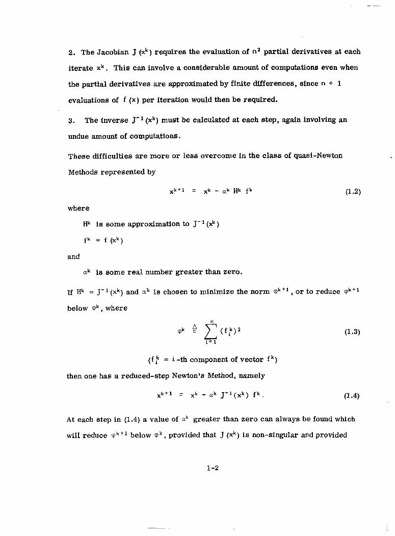
2. The Jacobian J (xk) requires the evaluation of n2 partial derivatives at each

iterate xk . This can involve a considerable amount of computations even when

the partial derivatives are approximated by finite differences, since n + 1

evaluations of f (x) per iteration would then be required.

3. The inverse J-l (xk)must be calculated at each step, again involving an

undue amount of computations.

These difficulties are more or less overcome in the class of quasi-Newton

Methods represented by

x k + l = Xk - uk Hk f k

where

Hk is some approximation to J' (9)

fk = f (Xk)

and

uk is some real number greater than zero.

If Hk = J-' (xk)and ak is chosen to minimize the norm cpk+l,o r to reduce q k + l

below c p k , where

( f = i -th component of vector fk)

then one has a reduced-step Newton's Method, namely

x k + l xk - uk J-l(Xk) f k .

At each step in (1.4)a value of uk greater than zero can always be found which

wi l l reduce q k + lbelow cpk ,provided that J (xk)is non-singular and provided

1-2

that f (xk) # 0. This is easily proved by showing that the direction of Axk given

by (1.4),namely - J' '(xk) f k ,has a component along the negative gradient of rpk ,

i.e., by showing that

(grad'cpk, J''(xk) f k ) > 0 .

One has

or

grad rpk = 2 JT(xk) f k .

Then

This reduced-step Newton's Method, with ak selected to reduce r p k + ' below r p k ,

will converge to a solution of f (x ) = o for any starting value in a region

bounded by the contour rp = constant, i f a solution exists in this region and i f

J-' (x)exists everywhere in this region. This region of convergence is as large

o r larger than that in the standard (full-step) Newton's Method so that the dis­

advantage of a small region of convergence often encountered in the full-step

Newton's Method is somewhat alleviated by the reduced-step variant. However, , the reduced-step version still has the disadvantages 'of requiring the calculation

of J (xk)and its inverse at each step.

1-3

The Method of Steepest Descent, o r Gradient Method (see e.g., [ 111, [ 161, [ 171,

[ 19]), for solving f (x) = 0 can be regarded as a quasi-Newton method by

letting Hk = J T (xk), with uk selected to minimize o r reduce the norm q k t l .

Thus one has

Note that grad cpk = 2 JT(xk)f k so that the direction of A xk given by (1.8) is

along the path of steepest descent. Thus a value of ak > 0 can always be found

to reduce v k t l below vk as long as JT(xk) f k # 0. Assuming J (xk)is non­

singular, f f 0 implies J T (xk) f # 0. In addition, we can sometimes satisfy

JT(xk) f k # 0 even though J (xk) is singular. Thus the region of convergence in

the Gradient Method is as large o r larger than that in the reduced-step or regular

(full-step) Newton's Method. In addition, this method eliminates the need to

calculate the inverse of J (xk). However, the Gradient Method lacks the quadratic

convergence of Newton's Method. Its behavior near a solution of f (x) = 0 i B

rather oscillatory in general.

A method which combines the feature of the larger region of convergence inherent

in the Gradient Method together with the quadratic convergence of Newton's

Method near a solution, is Marquardt's Algorithm [ 141 ,

As hk - 0, (1.9) becomes Newton's Method, while hk - yields the Gradient

Method. In general, a small value of Ak is sought in order for the method to

approach the quadratic convergence of Newton's Method, and Ak is increased

only as necessary to satisfy

.

1-4

q++l < cpk , (1-10)

which is the basic criterion that muet be satisfied at each step. While the con­

vergent properties of Marquardt's algorithm are improvements over those in

Newton's Method alone o r the Gradient Method alone, the algorithm requires

considerably more computations at each step than either of the latter two

methods.

If H k = .J"(x') and ak = 1,one obtains the simplified Newton's Method,

X k + l = Xk - J'l(xl) f k . (1.11)

This simplified Newton's Method eliminates the need for frequent calculation

of J (xk) and its inverse. In general, this method does not converge as rapidly

as Newton's Method. In particular, it lacks the quadratic convergence of Newton's

Method, unless by some odd chance, J (L) = J (x ') where is the solution. In

addition i t suffers, in common with Newton's Method, the fault of a small region

of convergence in many problems. This fault can be alleviated somewhat, as

w a s done for Newton's Method, by a reduced-step version, namely,

(1.12)

where ak is chosen to minimize rpk" or to satisfy the condition

q++l < c p k . (1.13)

< The Secant Method [ 21 , [ 16J can be expressed as a quasi-Newton method in

Awhich ak = 1and Hk = (Jk) - ' is the inverse Jacobian of the equivalent linear

system corresDonding. to the last n + 1 points. It is a Feneralization of the

1-5

Secant Method in one dimension, in which a straight line is passed through the

two points (xk, f k ) and (xk'l, fk - l ) ; the intersection of this line with the x axis

determines xk 'l . Thus in n dimensions, one has

X k + l = xk - ( J k ) - 1 f k . (1.14)

The matrix Jk (or (Jk)- l ) is determined from the requirement that

f i = Jk [xi - x*], i = k, k - 1, . . . , k - n (1.15)

where x* P x k + lis the next estimate of the solution. Letting

n x i 4- x i + l - x i (1.16)

and

& 1 . 4

equation (1.15)yields

A f i = Jk A x i , i = k - 1 , k - 2 , . . . , k - n . (1.17)

JWith the n x n matrices A Xk and nFk defined as

nA x k = [ A X k - n . . . A ~ k - 2A x k - 1 1 (1.18)

and

equation (1.17)yields

(1.19)

or

1-6

L

(assuming (A Xk 1- ' exists)

(1.20)

(assuming (A Fk )- * exists).

Thus, solving equation (1.20)for (Jk)- l and substituting in (1.14)yields x k t l ,

the next estimate of the solution to f (x) = 0, after,which the process is repeated.

The Secant Method is defined even if A X k is singular, since the existence of Hk

requires only that (AFk) - l exists. However, if A X k is singular (implying Hk is

singular), then it can be shown that the iteration cannot converge to a solution

except under specialized conditions. Note that J k in the Secant Method is not

the same as J ( x k ) in Newton's Method. The latter represents the Jacobian at a f ;

the point x k (formed from n partial derivatives a,.evaluated at x = x k ) while J

J k is the Jacobian of the linear system (1.15)that interpolates the n 3- 1points

(Xk , f k ) , ( x k - 1 , f k - I ) , ..., (Xk'", f k - " ) .

An equivalent representation of the Secant Method is obtained by defining

8 xi 4 Xk - x i , 8 f i 4 f k - f i (1.21)

i = k - l , k - 2 , . . . , k - n

and n x n matrices 8 Xk a n d 8Fkas

6 xk P [s x k - " . . . 8 x k - 2 8 Xk- (1.22)

and

1-7

Then equation (1.15) yields

6 f i = Jk Ex i , i = k - 1, . . . , k - n

S F k = J k 6 P

or

J k = 6 Fk (6Xk))'l

(assuming (6 Xk1- ' exists)

and

(1.23)

(1.24)

(1.25)

(assuming (6Fk)-' exists).

The ,matrix J k and its inverse, defined by (1.24)and (1.25),are the same as the

corresponding ones obtained from (1.19)and (1.20),since both representations

a re derived from the same linear system (1.15);assuming the existence of the

required inverses, n + 1 points (xi,f i, uniquely define the parameters of an

n-th order linear system. It is also easy to show that (6Xk) - l exists if and only

if ( A X k ) - ' exists and that (6Fk)-'exists if and only if ( n F k ) - l exists. Thus

equations (1.25) and (1.14) form an equivalent representation of the Secant

Method.

The Secant Method avoids the necessity of calculating J (xk) (and its n 2 partial

derivatives) at each step but still requires (in the quasi-Newton form of the

Secant Method) a matrix inversion and multiplication at each step. The Secant

Method has local superlinear convergence provided the last n vectors Axi

1-8

forming AXk remain sufficiently independent (see Section III). But there is no

way of insuring that this condition is met at every step, so that convergence, let

alone superlinear convergence, is not assured in general. Even when local con­

vergence occurs, the region of convergence may be rather limited in many

problems as is the case for the full-step Newton's Method. Again, this region

can be enlarged in the reduced-step version, namely

X k + l = Xk - a k ( J k ) - l fk (1.26)

with (Jk)-l determined as before from (1.20) or (1.25) and ak selected to satisfy

(1.13).

Probably the greatest drawback of the Secant Method is the numerical instability

and lack of convergence resulting from near singular matrices A X k and AFk.

This occurs when A x k - (A f k' l ) is "nearly" a linear combination of the previous

n - 1vectors. The matrix Jk determined from such near singular matrices

fails to approach J (xk)at the solution, thus ruining the theoretical convergence

of the Secant Method.

It is not necessary to calculate J k or i ts inverse explicitly in the Secant Method

in order to solve for x* = xkt l , the next estimate of the solution. Following

Wolfe's derivation [ 251 ,one can denote the last set of n + 1points by (xl,f l),

(x2, f 2 ) , ..., ( X " t 1 , fnt l), Then equation (1.15)would read

f i = J(x1 - x*), i -- 1, 2 . . . , n + l (1.27)

where J is the matrix of the linear system corresponding to these n + 1points

(xi,f ). Since the n + 1vectors f must be linearly dependent, there exist con­

stants n i not all zero such that

1-9

n + 1 7ri f ' = 0.

One can normalize.the constants r i such that

n + l

ni = 1.

Utilizing equation (1.27) in (1.28), and multiplying by J"

exist, one obtains

n + 1c 7ri (xi - x*) = 0.

Solving for x* (noting that Z *i = 1) yields

n + 1 x* = Ti xi *

i = l

(1.28)

(1.29)

which is assumed to

The n + 1 constants v i can be obtained from equations (1.28) and (1.29).

the (n + 1) x (n+ 1) matrix A defined as

and the (n + 1)-vector 7~ as

equations (1.28) and (1.29) can be written as

A l l = [ o o . . . 0 1 I T

(1.30)

(1.31)

With

(1.32)

(1.33)

(1.34)

1-10

n = A-1 [0 0 . .. 0 1 I T (1.35)

Equations (1.35)and (1.31)yield x*, the next estimate of the solution. Wolfe

suggests using the pair (x*, f (x*)) to replace the pair (x j , f j ) for which the

norm CP' 4 ( f i)T f i is a maximum. Denoting the new matrix of (1.32)as A* (in

, which f (x*) has replaced f j ), he uses the Sherman-Morrison modification

method [ 121 , [ 201 to obtain a simplified formula for calculating (A*)' based on

knowledge of the previous inverse, A' l .

This version of the Secant Method has several drawbacks. For one, the matrix J

is not explicitly calculated, and in some problems it is necessary or desirable

to obtain an approximation to the Jacobian of the system at the solution. Sec­

ondly, it is inherently a full-step Secant Method; it does not lend itself to the

introduction of a constant ak different from unity. Thus the norm reducing

feature of the reduced-step method, which can enlarge the region of convergence,

is not available in this version. Finally, the matrix A often becomes ill-conditioned

as w e approach a solution, resulting in the same degraded convergence or lack of

convergence near the solution that afflicts other versions of the Secant Method.

This problem can be alleviated in the proposed variants of the Secant Method,

where (Jk)-' is available at each step. This wil l be discussed later.

Barnes' version of the Secant Method [ 11 starts with an initial estimate J of

the Jacobian, and develops corrections to the estimated Jacobian J at each step

as

J k + l = J k + Dk (1.36)

1-11

where

D k = f k + l ( z k ) T

( z k ) = A xk

and A xk is obtained in the usual way (e.g., see (1.14)) from

Jk Axk = - f k . (1.37)

If k 5 n , the vector zk at each step is selected to be orthogonal to the previous

(k - 1)vectors Ax , Ax2, ...,Axk''. If k > n, zk is selected to be orthogonal to

the previous n - 1 vectors AX^'^' l , ...,Axk". The result of this choice, using

(1.36),is that

@ A x i = 0, O < k - i < n

and

J k + l A x ' = Jk o x i , 0 < k - i < n .

Since (1.39)is true for any k such that 0 < k - i < n ,this implies that

J k + l n x i = Jk n x i = J k - 1 A x i = . . . = J i + l A x ' .

Utilizing (1.36) once more, yields

J i + l nxi = J i A x i + f i + l

or

J i + l n x i = n f i

using equation (1.37). Hence, from (1.40)and (1.41),

J k n x i = A f ' , 0 k - i (ri.

(1.38)

(1.39)

(1.40)

(1.41)

(1.42)

1-12

If k > n, one has

11I Jk A x i = A f i , i = k - 1 , k - 2 , . . . , k - n (1.43)

This is exactly the same as equation (1.17) which forms the basis for the Secant

Method. Thus, in n iterations, starting from initial estimates J and xl,

Barnes' algorithm generates n + 1points (xl, f I ) , (x2, f2), ..., (xntl, f n t l ) and

a matrix J n + l which is the Jacobian of the linear system interpolating these

n + 1 points. Every subsequent iteration drops the earliest point and adds the

most recent one, modifying the J matrix to correspond to this most recent set

of n + 1 points. In other words, after n iterations Barnes' algorithm is exactly

I the same as the Secant Method as previously derived. 1

Barnes' algorithm has the advantage of not requiring an initial set of n + 1 points

in order to begin the Secant Method. It can begin with only initial estimates J

and x1 and form as a matter of course the n + 1 points leading to the regular

Secant Method. Of course, the better the initial estimate J ' , the faster wi l l be

the convergence in general. For a linear system the algorithm wi l l theoretically

converge to a solution of f (x) = 0 within n + 1 iterations, regardless of the

1 initial estimate J ', since the matrix J"' corresponding to the n + 1 points

11 (xl,f ' ), . . . .. ., (x"", f"'') completely defines the linear system; the next tf (n + 1) application of (1.37) (with k = n + 1)yields the solution of the linear

1 system f (x) = 0. Barnes' algorithm has the disadvantage of requiring the solu­

tion of 11 linear equations at each step (in solving (1.37)for axk), which is almost

equivalent to requiring the inversion of J k at each step. It also, in its original

form, represents a full-step Secant Method (uk = 1) so that its region of con­

vergence is restricted compared to the reduced-step version.

1-13

1 -

-

Rosen's modification [ 181 of Barnes' algorithm eliminates these last two disad­

vantages. In addition to restructuring the algorithm as a reduced-step method,

Rosen formulates the algorithm to update (Jk)-l directly rather than J k . This

is accomplished as follows. Let

Axk - - a k ( J k ) ' l f k (1.44)

corresponding to a reduced-step method, and let the correction to J k be repre­

sented as

where

D k -4 ( A f k - J k A x k ) ( z ~ ) ~ ...~ ..­

( ~ k ) ~A xk

With zk selected as in Barnes' algorithm, this yields the reduced-step Secant

Method after n iterations, in the same way that Barnes' original algorithm

produced the full-step version. However, instead of updating J k as in (1.45),

Rosen uses the Sherman-Morrison modification formula [ 121 , [ 201 to convert A(1.45) into an updating of Hk = (Jk)- l. Thus, one obtains

H k + l = Hk + (xk - Hk f k ) (zk)= Hk - (1.46)

f k ­

where

Thus Hkt can be calculated fairly simply from a knowledge of Hk . Then A xk

can be calculated directly from (1.44)without the need for solving a set of n

linear equations o r of completely recalculating the inverse of J k at each step.

1-14

The Rosen-Barnes algorithms do not solve the problem of numerical instability

inherent in the Secant Method whenever the matrix A x k + l (or AFk+l )becomes

ill-conditioned as a result of A xk (or A f k ) being %earlyt1 a linear combination

of the previous n - 1vectors. In the Barnes algorithm, the first condition m a i ­1d.fi

fests itself whenever

(1.47)

where E is some small positive number. This condition would raise doubts as

to the validity of the results obtained in ca lcu la t iq J k + l from equation (1.47).

In Rosen's modification, the second condition would be evident whenever

(1.48)

where E ' is some small positive number. Again, this condition would detract

from the reliable computation of from (1.46). Barnes considers the problem

i and suggests rejecting the vector Axk whenever the condition of equation (1.47) , , occurs. He claims that a satisfactory alternative is to select a A x k for this step

, so as to result in z being parallel to A xk . Of course this cures the numerical

problem associated with the reliable computation of J k + l . However, it does little

to insure fast convergence to a solution of f (x) = 0 since the direction of the

selected A xk would be quite different from the presumably optimum direction

' suggested by the previous value of Jk . Broyden's algorithms [ 41 form another quasi-Newton method, which can be

related to the Rosen-Barnes version of the Secant Method. Broyden's Method 1

algorithm (which he found to be effective) is

1-15

I

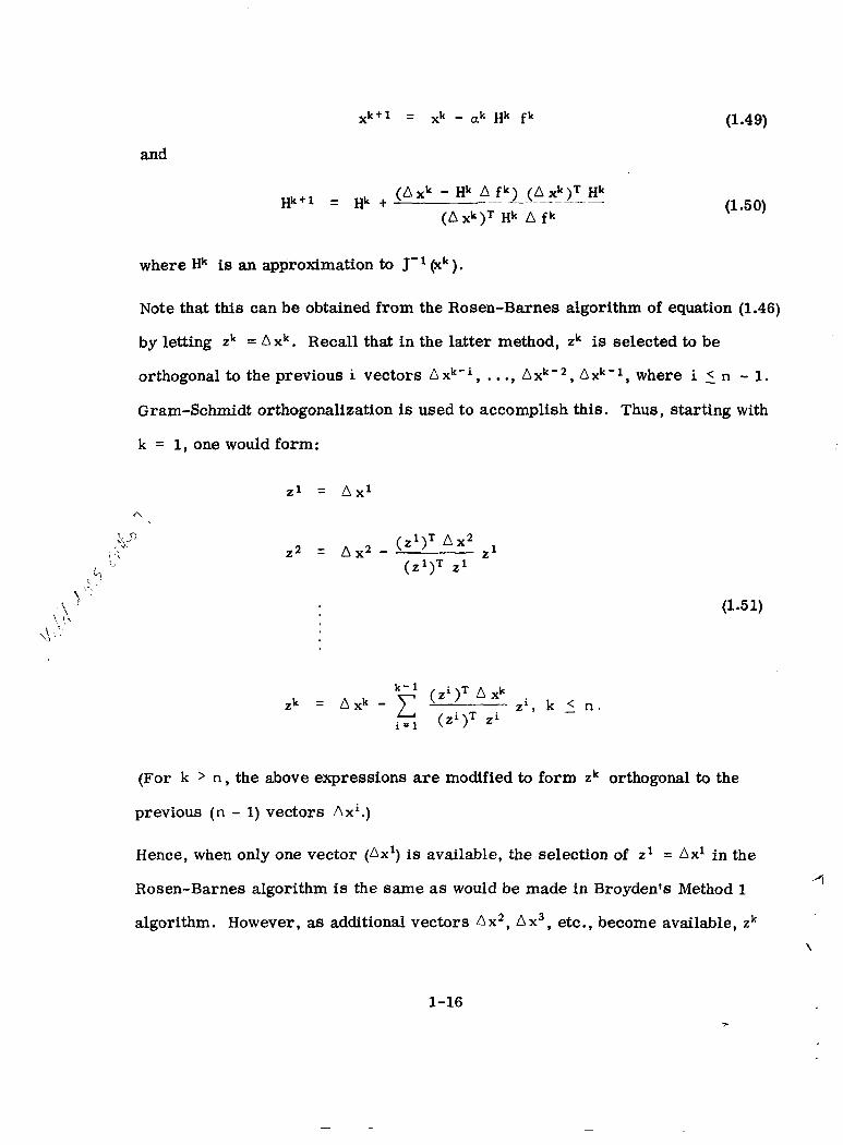
X k + l = Xk - ,k Hk f k (1.49)

and

(1.50)

where Hk is an approximation to J-' (xk).

Note that this can be obtained from the Rosen-Barnes algorithm of equation (1.46)

by letting zk = A xk. Recall that in the latter method, zk is selected to be

orthogonal to the previous i vectors AX^'^, ..., AX^'^, Axk'l, where i 5 n - 1.

Gram-Schmidt orthogonalization is used to accomplish this. Thus, starting with

k = 1,one would form:

(1.51)

zk = A x k -k -C1 ( z ' ) ~Axk

z i , k 1. n . i = l ( Z ' y zi

(For k > n , the above expressions are modified to form zk orthogonal to the

previous (n - 1)vectors Ax'.)

Hence, when only one vector (Ax') is available, the selection of z1 = Ax1 in the

Rosen-Barnes algorithm is the same as would be made in Broyden's Method 1 1

algorithm. However, a8 additional vectors Ax2,Ax3, etc., become available, zk

\

1-16

A the Rosen-Barnes algorithm are formed from (1. l),whereas Broyden's

algorithm continues to use zk = A x k . The choice of zk as per equation (1.51)

results in the Rosen-Barnee algorithm evolving into the Secant Method after n

iterations, so that for a linear system the matrix Hnt equals J' I , the inverse

Jacobian of the system, and the next (n + 1)application of equation (1.44) results

in the solution of the linear system f (x) = 0. There is no such assurance in

Broyden's algorithm that the method will converge in n + 1 iterations for a linear

system, or even converge at all, although subsequent work by Broyden [ 61 estab­

lishes conditions under which his method converges for linear systems. Numeri­

cal experience seems to indicate that Broyden's Method 1algorithm is effective C l

8 in a wide variety of problems, especially if the initial estimate H' of the inversed 4 Jacobian is a good one, and/or the initial estimate x1 is close to the solution.1

If this is not the case, the Rosen-Barnes algorithm is considered to be more

effective.

Rosen indicates that on a particular test problem, better results were obtained

using a zk that was the average of that obtained from his algorithm with the zk

obtained from Broyden's algorithm, than were obtained using either procedure

alone. This author is inclined to think that one of the reasons for this is that

Broyden's algorithm inherently avoids the numerical problems evidenced by the

occurrence of condition (1.47). In fact, for Broyden's algorithm,

(1.52)

since z k = a x k . The average of the zk 1s from the two methods wi l l consistently

avoid the condition of (1.47). At the same time, this average may still produce

1-17

a fair representation of the linear system corresponding to the previous

points.

Broyden's Method 2 cqnsists of equation (1.49) together with

Hk+1 = Hk +. ( A xk - Hk A f k ) (A f k ) T

(A f k ) T A f k (1.53)

where Hk is again an approximation to the inverse Jacobian. Equation (1.53)

can be obtained from (1.46)by letting

( ~ k ) ~ = ( A f k ) T . (1.54)Hk

Equation (1.53) can also be derived from Zeleznik's form of a generalized

quasi-Newton Method 1261, namely equation (1.49) combined with

(1.55)

Letting uk = vk = O f k results in (1.53). Zeleznik shows that for a linear system,

in order for (1.55) to converge to the inverse Jacobian within n iterations, the

following conditions must be satisfied.

But, as Zeleznik points out, the choice of uk = vk = A f k gives no assurance of

meeting (1.56);hence there is no assurance that Broyden's Method 2 will con­

verge even for a linear system. However under certain conditions, namely

when 1) I - AHko ) I 2 < 1 at some instant k, , it is easy to show that for ukE (0;I]

1-18

I

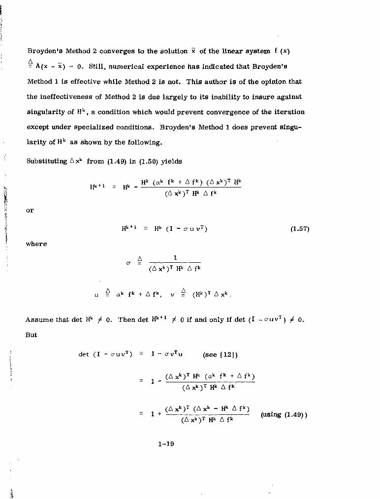
Broyden's Method 2 converges to the solution X of the linear system f (x) -9A(x - x ) = 0. Still, numerical experience has indicated that Broyden's

Method 1is effective while Method 2 is not. This author is of the opinion that

the ineffectiveness of Method 2 is due largely to its inability to insure against

singularity of ti", a condition which would prevent convergence of the iteration

except under specialized conditions. Broyden's Method 1does prevent singu­

larity of Hk as shown by the following.

I Substituting A xk from (1.49) in (1.50) yields

H k + l = Hk - Hk ( a k f k t A f k ) AX^)^ Hk

(A x ~ ) ~Hk A f k

..i Hktl = Hk ( I - a u v T ) (1.57)'i where

c r 4 1 AX^)^ Hk A f k

u =A ,k f k t A f k , v (Hk)T A x k .

Assume that det Hk # 0. Then det Hk+' # 0 if and only if det (I - cruvT) # 0.

But

det (I - auvT) = 1 - u v T u (see I121 ) ! h

1 = 1 - ( A x " ) T Hk (uk f k + A f k )

AX^)^ Hk A fk

AX^)^ ( A X " - Hk A f " ) = I +

(Axk)= Hk A f k (using (1.49))

1-19

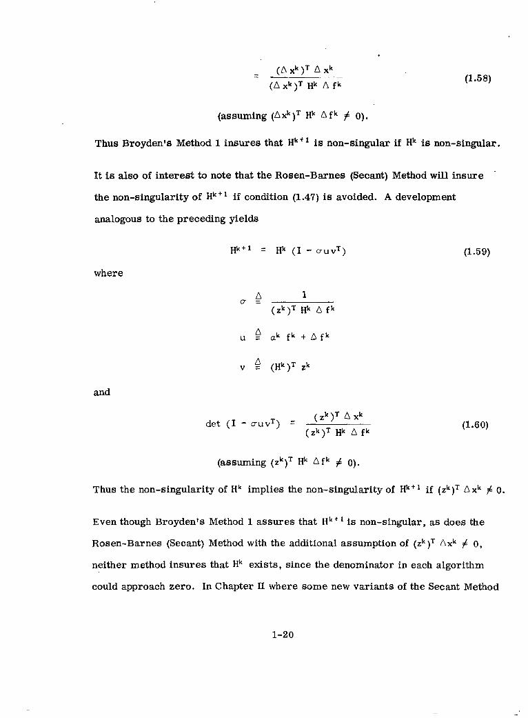
AX^)^ xk-- .= ~ -

AX^)^ Hk A f k (1.58)

(assuming AX^)^ Hk A f k f 0) .

Thus Broyden's Method 1insures that Hk " is non-singular i f Hk is non-singular.

.It is a160 of interest to note that the Rosen-Barnes (Secant) Method wi l l insure

the non-singularity of Hk '' i f condition (1.47) is avoided. A development

analogous to the preceding yields

H k + l = Hk (I - a u v T ) (1.59)

where

and

det ( I - cruvT) = ( z k ) T A x k

Hk( ~ k ) ~ A fk (1.60)

(assuming ( zk)T Hk A f k # 0).

Thus the non-singularity of Hk implies the non-singularity of Hkt if ( z ~ ) ~A x k f 0.

Even though Broyden's Method 1assures that H k + l is non-singular, as does the

Rosen-Barnes (Secant) Method with the additional assumption of ( z ~ ) ~Axk # 0,

neither method insures that Hk exists, since the denominator in each algorithm

could approach zero. In Chapter II where some new variants of the Secant Method

1-20

are presented, it wi l l be shown that the algorithm denoted as Algorithm II

insures that Hk both exists and is non-singular.

There are many other methods for solving f (x) = 0 including two-point secant

methods (as opposed to the (n + 1)-point secant method which is simply called

the Secant Method in this report) and Steffensen's methods [ 161, [241 . Both of

these classes of methods exhibit superlinear convergence (1.61 and 2 respec­

tively). But, like the discrete Newton's Method, they generally require n + 1

function evaluations and a matrix inversion per iteration. The system f (x) = 0

can also be solved by any of a number of minimization techniques [ 161 , since

solution of f (x) = o is equivalent to minimizing cp (x) 2 fT(x) f (x) (to zero).

A relatively simple minimization technique is the Fletcher-Powell-Davidon

Method [ 71. Finally, there a re more complex methods, such as the Freudenstein-

Roth Method [ 81 , for solving f (x) = 0 in the difficult case where the Jacobian is

singular at points in any region connecting the starting estimate with the solution.

The other methods mentioned are ineffective in this case.

The remainder of this report will concern itself with some new variants of the

Secant Method. These variants were developed to overcome the previously dis­

cussed limitations of existing versions of the Secant Method.

1-21

SECTIONS II

ALGORITHMS I AND 11

2.1 INTRODUCTION

Algorithms I and I1 are variants of the Secant Method for solving f (x) = 0, n

nonlinear equations in n unknowns. These algorithms are designed to avoid

some numerical problems that can cause poor convergence in the Secant Method.

The complex ser ies of steps leading to their development wil l be omitted; rather

the final form of the algorithms will be presented and analyzed.

Both algorithms follow the quasi-Newton iteration

X k + l - Xk A X k = - a k Hk f k

where ak is either selected a8 unity (full step version) or else BO as to insure

that

( p k + l < (pk (2 4 where

rpk 4 ( f k ) T f k .

The matrix Hk , representing an estimate of the inverse Jacobian at x k , is formed

to satisfy

AX: = Hk Af:, i = 1, 2, . . . ( mk

mk I n.

The vectors Ax! are certain previous difference vectors A x j , j < k ,formed

2-1

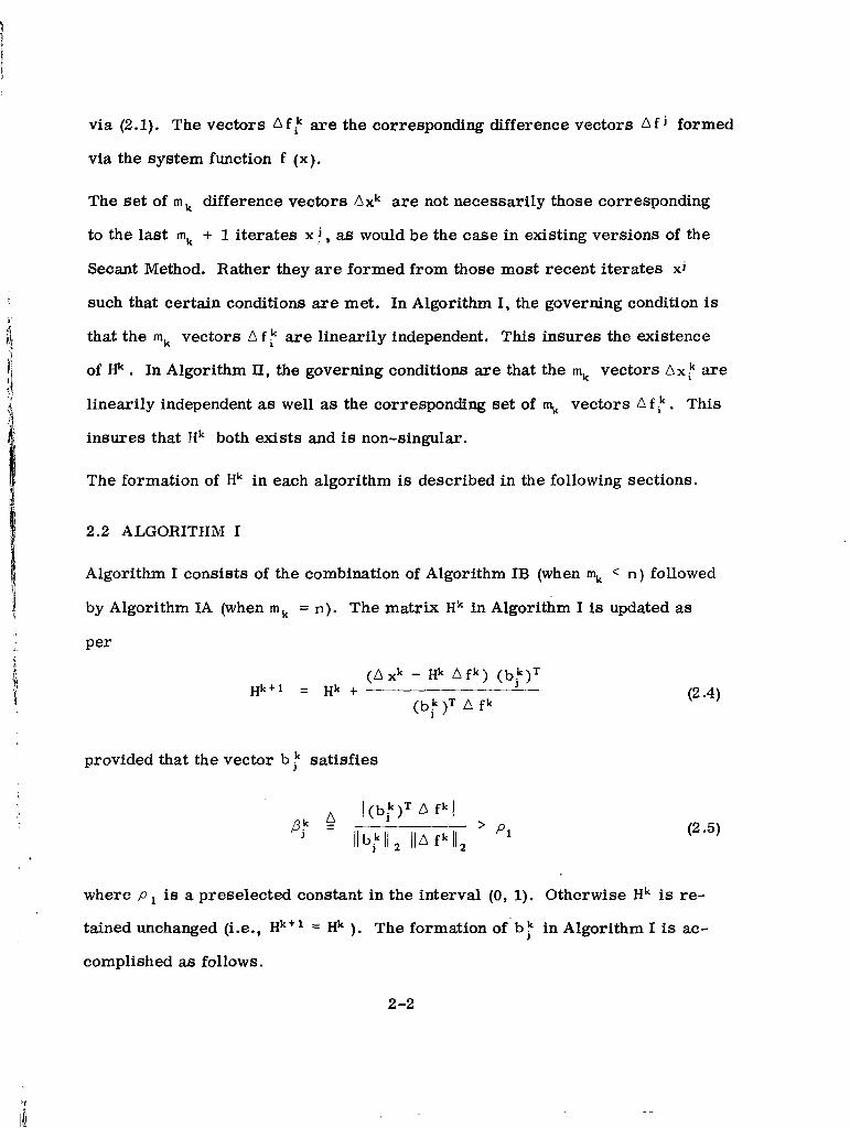
via (2.1). The vectors O f f are the corresponding difference vectors O f 1 formed

via the system function f (x).

The set of m k difference vectors Axk are not necessarily those corresponding

to the last mk + 1iterates x J ,as would be the case in existing versions of the

Secant Method. Rather they are formed from those most recent iterates xJ

such that certain conditions are met. In Algorithm I, the governing condition is

that the mk vectors A f are linearily independent. This insures the existence

of Hk . In Algorithm 11, the governing conditions are that the mk vectors AX! are

linearily independent as wel l as the corresponding set of % vectors A f k . This

insures that !Ik both exists and is non-singular.

The formation of Hk in each algorithm is described in the following sections.

2.2 ALGORITHM I

Algorithm I consists of the combination of Algorithm IB (when % < n ) followed

by Algorithm IA (when mk = n). The matrix Hk in Algorithm I is updated as

Per

(A Xk - Hk A f k ) (br)THkt1 = Hk +

(bF)T 0 f k

provided that the vector b r satisfies

where P is a preselected constant in the interval (0, 1). Otherwise Hk is re­

tained unchanged (i.e., Hk+l= Hk ). The formation of 'b$ in Algorithm I is ac­

complished as follows.

2-2

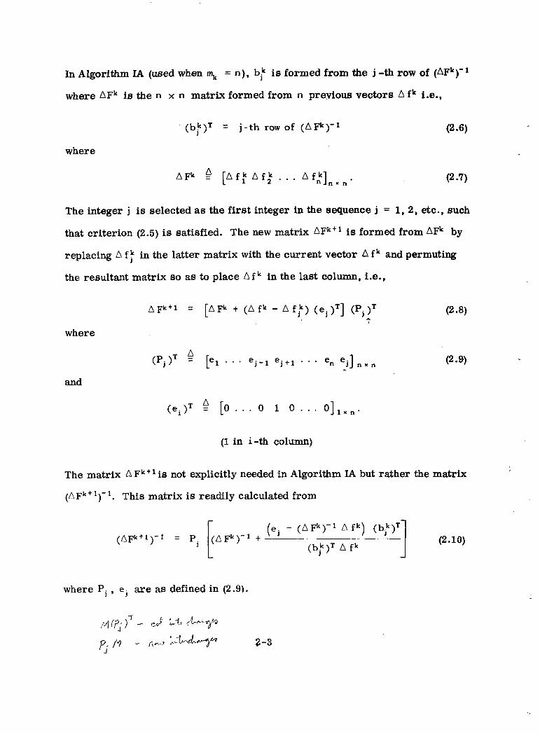
In Algorithm IA (used when mk = n), bf is formed from the j -th row of (AFk)'I

where A F k is the n x n matrix formed from n previous vectors A fk i.e.,

.,(b:)T = j - th row of ( A F k ) - l

where

=A F k A [ A f : A f i . . . A f ; I n x n . (2 -7)

The integer j is selected a s the first integer in the sequence j = 1,2, etc., such

that criterion (2.5)is satisfied. The new matrix AFkt is formed from AFk by

replacing A f in the latter matrix with the current vector A f k and permuting

the resultant matrix so as to place A f in the last column, Le.,

n ~ k + l = [AFk t (A f k - A f f ) (ej)T] (Pj)T (2.8)T

where

( P ~ ) ~ [e, . . . e j - , e j t l . . . e n ej] n x n (2.9)

and

(ei>' P [o.. . o 1 0 . .. 0 1 , ~ ~ . (1 in i-th column)

n =

The matrix A Fk"is not explicitly needed in Algorithm IA but rather the matrix

(A Fkt ,)- '. This matrix is readily calculated from

(ej - ( A F k ) - ' A f k ) (b.:)T ( A F k ) - I +

(b:)T A f k 1 (2.10)

where Pj , e j are a s defined in (2.9).

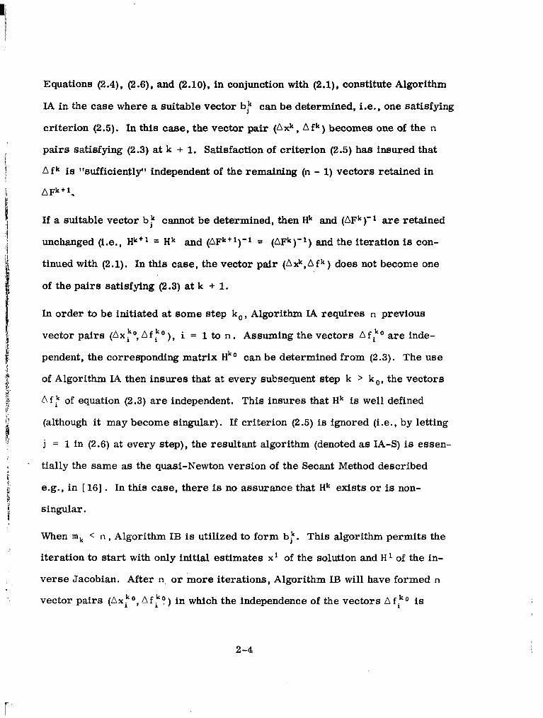
Equations (2.4), (2.6),and (2.10), in conjunction with (2,1),constitute Algorithm

LA in the case where a suitable vector bl can be determined, i.e., one satisfying

criterion (2.5). In this case, the vector pair ( A x k , A f k ) becomes one of the n

pairs satisfying (2.3) at k + 1. Satisfaction of criterion (2.5) has insured that

A f k is "sufficiently" independent of the remaining (n - 1)vectors retained in

AFk+l, .

If a suitable vector bf cannot be determined, then Hk and (AFk) - l are retained

unchanged (i.e., Hktl = Hk and (AFktf)' l = ( A F k ) - l ) and the iteration is con­

tinued with (2.1). In this case, the vector pair ( A x k , A f k ) does not become one

of the pairs satisfying (2.3) at k + 1.

In order to be initiated at some step k,, Algorithm LA requires n previous

vector pairs ( A x F o , A f F o ) , i = 1 to n . Assuming the vectors Af"O a re inde­

pendent, the corresponding matrix Hko can be determined from (2.3). The use

of Algorithm IA then insures that at every subsequent step k > k,, the vectors

A f of equation (2.3)are independent. This insures that Hk is wel l defined

(although it may become singular). If criterion (2.5)is ignored (i.e., by letting

j = 1 in (2.6)at every step), the resultant algorithm (denoted as IA-S) is essen­

tially the same as the quasi-Newton version of the Secant Method described

e.g., in [ 161. In this case, there is no assurance that Hk exists o r is non­

singular.

When m k < n ,Algorithm IB is utilized to form br. This algorithm permits the

iteration to start wi th only initial estimates x of the solution and H of the in­

verse Jacobian. After n. o r more iterations, Algorithm IB wil l have formed n

vector pairs ( A x k O , A f :I)) in which the independence of the vectors A fko is

2-4

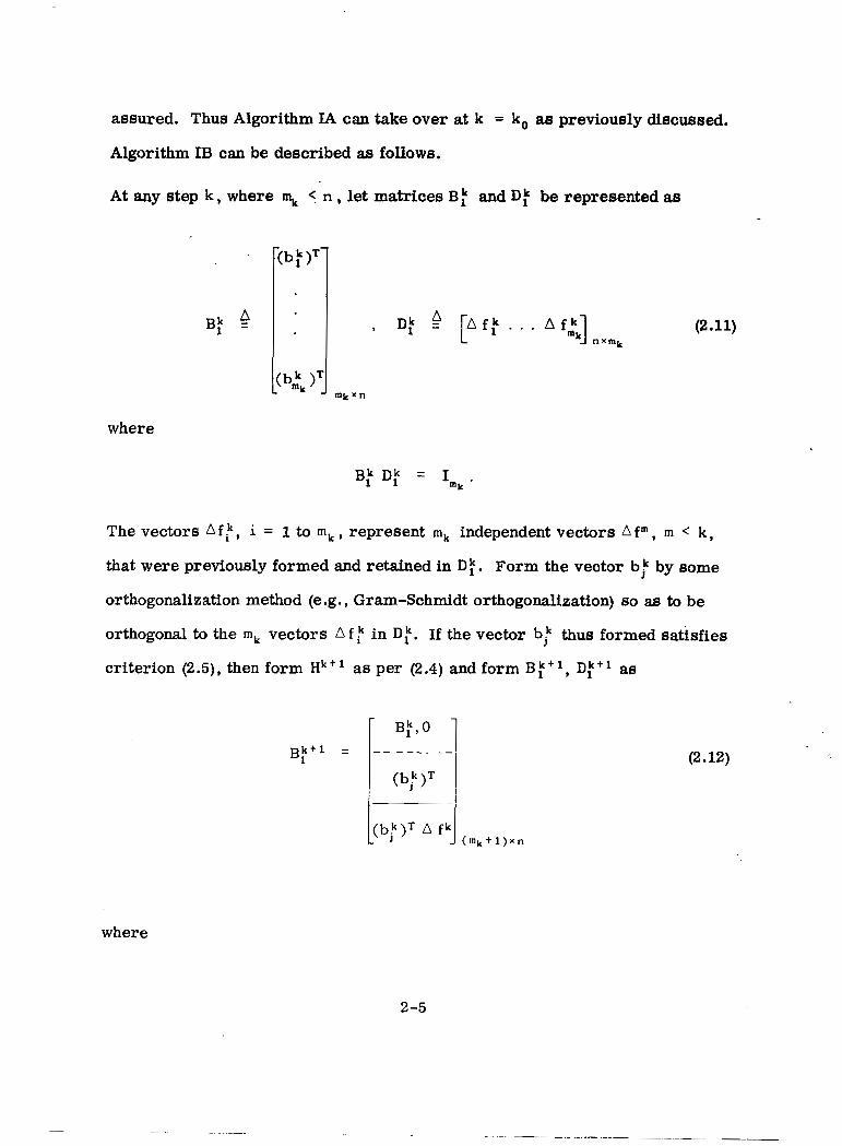
assured. Thus Algorithm IA can take over at k = k, as previously discussed.

Algorithm IB can be described as follows.

At any step k ,where Q < n ,let matrices B f and Dt be represented as

(2.11)

where

The vectors nfk, i = 1 to m k , represent mk independent vectors A f m , m < k ,

that were previously formed and retained in Di. Form the vector b: by some

orthogonalization method (e.g., Gram-Schmidt orthogonalization) so as to be

orthogonal to the mk vectors nfk in D:. If the vector b r thus formed satisfies

criterion (2.5), then form Hk" as per (2.4) and form B:", Df" as

(2.12)

where

2-5

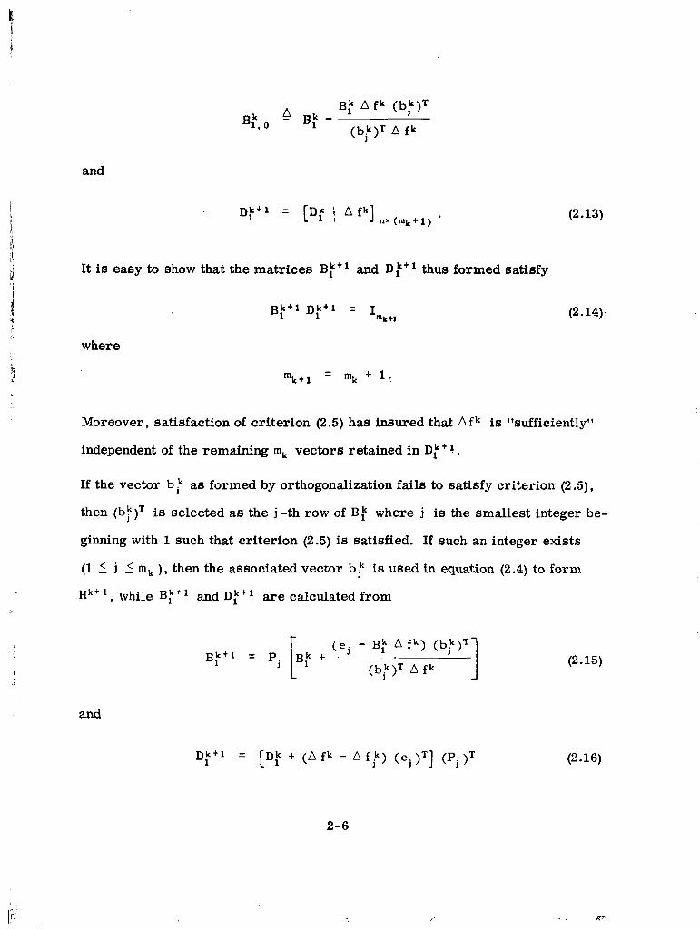
BF,o k Bf -B: A f k (br)T

(br)T A f k

and

(2.13)

It is easy to show that the matrices B:' and D :+thus formed satisfy

B k t l D k t l = I 1 1 mkt1

(2.14).

where

Moreover, satis,dction of criterion (2.5)has insured Lat fk is ffsufficientlyff

independent of the remaining mk vectors retained in D:' 1.

If the vector b l as formed by orthogonalization fails to satisfy criterion (2.5),

then (br)T is selected as the j -th row of BF where j is the smallest integer be­

ginning with l such that criterion (2.5) is satisfied. If such an integer exists

(1I j 5 m k ), then the associated vector bf is used in equation (2.4) to form

H k t ', while B:' and D:' are calculated from

( e j - B: A fk) (br)TBf'l = Pj [B: f

(br)T A f k 1 (2.15)

and

D:+1 = [D: t ( A f k - A f r > (ej)T] (Pj)' (2.16)

2-6

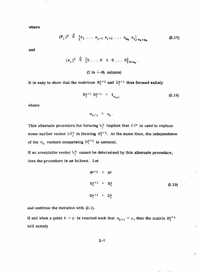
where

A(Pj>? = [e, . . . ej- l e j + l . . .

emk ej ] mkx.mk (2.17)

and

(1in i-th column)

It is easy to show that the matrices B,k+' and D:+' thus formed satisfy

(2.18)

where

-mk+ 1 - mk.

This alternate procedure for forming b: implies that A f k is used to replace

some earlier vector Afjk in forming D,k+l. At the same time, the independence

of the mk vectors comprising Df", is assured.

If an acceptable vector b: cannot be determined by this alternate procedure,

then the procedure is as follows. Let

(2.19)

and continue the iteration with (2.1).

If and when a point k = P is reached such that mk+ = n ,then the matrix B;+l

will satisfy

2-7

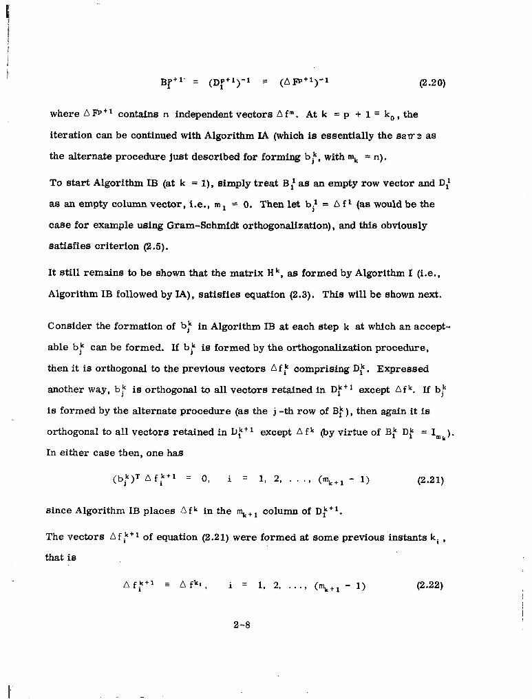
where A l?p+' contains n independent vectors A fm. At k = p + 1 k, ,the

iteration can be continued with Algorithm IA (which is essentially the saw 3 as

the alternate procedure just described for forming br, with mk = n).

To start Algorithm IB (at k = l), simply treat B l as an empty row vector and D:

as an empty column vector, Le., m l = 0. Then let bf = A f l (as would be the

case for example using Gram-Schmidt orthogonalization), and this obviously

satisfies criterion (2.5).

It still remains to be shown that the matrix H k , as formed by Algorithm I (i.e.,

Algorithm IB followed by IA), satisfies equation (2.3). This will be shown next.

Consider the formation of br in Algorithm IB at each step k at which an accept­

able b r can be formed. If br is formed by the orthogonalization procedure,

then it is orthogonal to the previous vectors A f comprising Dt . Expressed

another way, bp is orthogonal to all vectors retained in Df'l except A f k . If b/

is formed by the alternate procedure (as the j -th row of Bt ), then agdn it is

orthogonal to all vectors retained in LJft except A f (by virtue of Bf Df = Imk).

In either case then, one has

i(bf)T A f k t 1 = 0, i = 1, 2, . . . ) - l> (2.2 1)

since Algorithm IB places f in the % column of D f t l .

The vectors A f k t of equation (2.21)were formed at some previous instants ki ,

that is

2-8

... ..

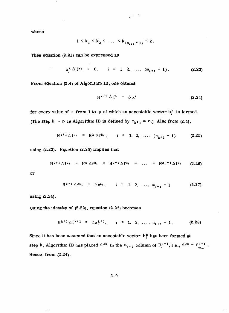
where

l ( k l < k, < . . . < k ( m k t l - 1) < k.

Then equation (2.21) can be expressed as

br A f k i = 0, i = 1, 2, * - - , - 1 ) . (2.23)

From equation (2.4) of Algorithm IB, one obtains

H k + l a fk = A x k (2.2 4)

for every value of k from 1to p at which an acceptable vector br is formed.

(The step k = P in Algorithm IB is defined by mk+ = n.) Also from (2.4),

H k + l A f k i = H k A f k i , 1 = 1, 2, * * . I ( m k + l - 1) (2.25)

using (2.23). Equation (2.25) implies that

H k t l A f k i = H k A f k i ,= H k - 1 A f k i = ... = H k i + l A f k i (2.2 6)

or

H k + l A f k i A x k i , i = 1, 2, . . . , %+I - 1 (2.27)

using (2.24).

Using the identity of (2.22), equation (2.27) becomes

H k + l A f k + l = A x k + l , i = 1, 2I . . . , % + 1 - l . (2.2 8)

Since it has been assumed that an acceptable vector br has been formed at

step k ,Algorithm .IB has placed A f k in the mk column of �3:' ',i.e., A f k = f k + 1 . mk+ 1

Hence', from (2.24),

2-9

, ~ k + l A f k + l -- Askk:: . m k t 1

Combining (2.28)and (2.29)yields

(2.29)

(2.30)

’ for every step k at which an acceptable vector br has been formed.

At any step k at which an acceptable vector br cannot be determined, Algorithm

IB utilizes equation (2.19)which implies that (2.30) is trivially true at this step

as well. Hence, equation (2.30)is true at every step k, which verifies that equa­

tion (2.3)holds for Algorithm IB. The proof for Algorithm IA follows directly,

since Algorithm IA can be derived from the alternate procedure of Algorithm IB

by letting mk = n.

Note that Algorithm IB has the same weakness as IA in that there is no assurance

that the vectors A x i , corresponding to the retained independent vectors A f i , are

themselves independent. Thus even though H k is always defined, it may become

singular. Once this happens, say at k = 4,Algorithm I will not be able to con­

verge to a solution K of f ( x ) = 0 unless the vector xq - X happens to be in the

subspace spanned by the columns of H q . This can be shown by the following,

which is similar to the development in [ 5 ] .

In both Algorithm IA and IB, H k+ can be written as

(Axk - Hk A f k ) (b:)T~ k + l = ~k +

(b:)T A f k

(ak f k + A f k ) (br)T

(br)TA f k I (using (2.l) ) I

2-10

or

where

Lk = 1 -(ak f k + A f k ) (br)TA -_____

(b:)T A f k

Then

(2.32)

where Hq is assumed to be singular. Hence from (2.l),

A x k + 1 = - , k + l H k + l f k + l

or

A ~ k ' l = HSv (2.33)

where

v 4 - , k t 1 L q L q + l . . . Lk f k + 1 .

Thus Axk+', which is some linear combination of the columns of Hq, is confined

to the subspace spanned by these columns, and this is true for every k 2 q. It

is also true obviously for Ax9 so that the iteration cannot possibly converge to

a solution 2 unless (xq - X) happens to lie in this same subspace.

If criterion (2.5) is ignored, the resultant algorithm (denoted a8 IB-S) is similar

to Zeleznik's construction [26]. The independence (or lack of independence) of

the vectors A f is ignored in this construction. Thus H k may not be defined

(in addition to having the risk of becoming singular as in Algorithm IB), causing - 1

obvious numerical problems. The combination of Algorithm IB-S followed by . LA-S forms a logical Secant Method algorithm, denoted a8 I-S, in which the inde­ . .

6

pendence of the vectors A f is consistently ignored.

2-11

I I

u"i ' . - Algorithm 11, to be discussed next, assures that the retained vectors A x i are

independent, as wel l as the corresponding vectors A f i . Thus the matrix Hk

remains well-defined and non-singular .

2.3 ALGORITHM 11

. Algorithm 11 consists of the combination of Algorithm IIB (when % < n) followed

by Algorithm IIA (when mk = n). The matrix Hk in Algorithm I1 is updated as

Per

( A x k - Hk A f k ) (a:)T Hk Hk+l = Hk + - - ~ = ~ (2.34)

(a:)T Hk A fk

'provided that the vector a: satisfies

(2.35)

and 1

(2.36)

\

where P , , p 2 a r e preselected constants in the interval (0, 1). Otherwise Hk is

retained unchanged (i.e., Hkt Hk ). The formation of a; in Algorithm 11is

accomplished as follows.

In Algorithm IIA (used when mk = n ) , a1k is formed from the j -th row of [AXk)-,

where A x k is the n x n matrix formed from the vectors A xf, i.e.,

(a:>' = j - th row of ( A X k ) - l (2.37)

2-12

I . . .

where

AAXk = [AX: A X ; . . . (2.38)

The integer j is selected as the first integer in the sequence j = 1,2, etc.,

such that criteria (2.35) and (2.36)are both satisfied. The new matrix A x k t is

formed from AXk by replacing A x ! in the latter matrix with the current vector

A xk and perm+ing the resultant matrix so as to place Axk in the last column,

i.e.,

A ) ( k t l = [ A S t ( A x k - A x : ) (ej)T] (Pj lT (2.39)

where Pj and e j are as defined in (2.9).

The matrix A x k t is not explicitly%eeded in Algorithm IIA but rather the

matrix (AXkt l)- l . This matrix is readily calculated from

where Pj and e are as defined in (2.9).

Equations (2.34), (2.37),and (2.40), in conjunction with (2.1), constitute Algo­

rithm IIA in the case where a suitable vector a: can be determined, i.e., one

slatisfying criteria (2.35)and (2.36). In this case, the vector pair (Ax: A f k ) be­

comes one of the pairs satisfying (2.3)at k + 1. If a suitable vector a: cannot

be determined, then Hk and (AXk)" are retained unchanged (i.e., H k + l Hk

and (AXkt l)- (AXk)- l ) and the iteration is continued with (2.1). In the latter

case, the vector pair ( A x k , A f k , does not satisfy (2.3)at k + 1.

. .

5

1

t

\

'?

-II

7­

2-13

1I A simpler algorithm naturally results if the criteria for independence, (2.35)

l

and (2.36),are ignored. This algorithm, denoted as IIA-S, is obtained by letting

j = 1in equation (2.37). It is another Secant Method algorithm similar to

Algorithm LA-S. Again, the existence and non-singularity of I l k are not assured

in this algorithm.

AS was the case with Algorithm IA, Algorithm IIA requires a.n initial set of n

vector pairs (Ax: O ,A f :' ), i = 1 to n . Again, the vectors A f ' must be inde­

pendent in order to define H k o from (2.3)J In addition, the vectors A x;O must be

independent in order that ( A X k O ) - l exist. The use of Algorithm IIA then insures

that at every subsequent step k > k, , the vectors A f : are independent as wel l

as the vectors Ax:. This insures that Hk is both defined and non-singular.

When mk < n ,Algorithm IIB is utilized to form a:. This algorithm permits the

iteration to start with only initial estimates x 1 of the solution and H' of the

inverse Jacobian. After n or more iterations, AlgorithdIB will have formed n

vector pairs (Ox:', A f k o ) in which the independence of the vectors A xk0 is

assured as well as that of the vectors A f k o . Thus Algorithm IIA can take over

at k = k,. Algorithm IIB can be described as follows.

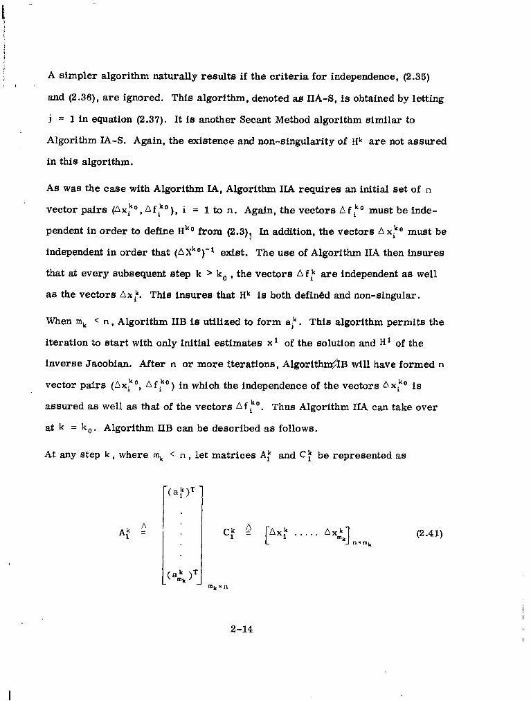
At any step k ,where mk < n , let matrices A: and C: be represented as

2-14 !

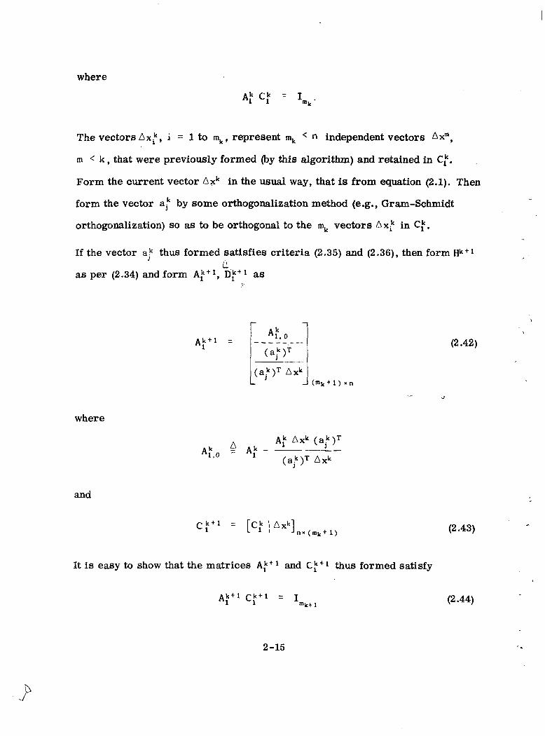
where

The vectors Ax!, i = 1to mk, represent mk < n independent vectors Ax"',

m < k ,that were previously formed (by this algorithm) and retained in Cf.

Form the current vector Axk in the usual way, that is from equation (2.1). Then

form the vector a; by some orthogonalization method (e.g., Gram-Schmidt

orthogonalization) so as to be orthogonal to the mk vectors Ax! in Ct . If the vector a; thus formed satisfies criteria (2.35)and (2.36),then form Hk+ 1

1.1

as per (2.34)and form >;+l as

(2.42)

.-J

where

and

C k . 1 = [c ; p x k ] n x ( m k + l ) (2.43)

It is easy to show that the matrices A;+1 and C:+l thus formed satisfy

m k t 1 (2.44)

2-15

aJ

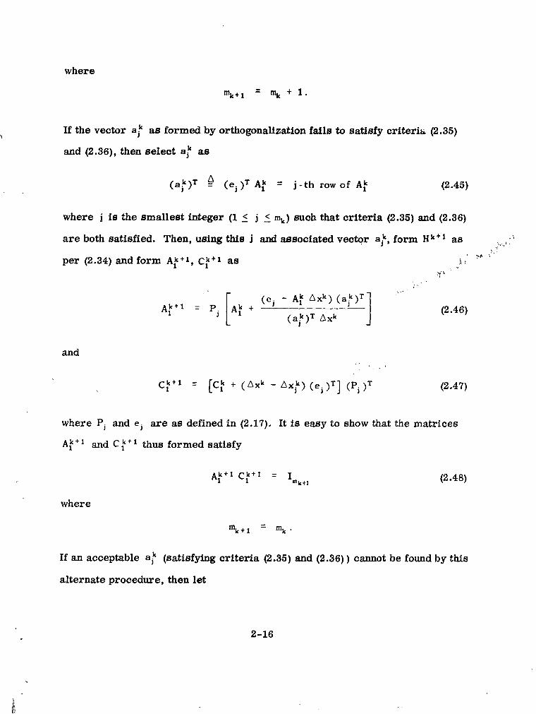
where

If the vector a/ as formed by orthogonalization fails to satisfy criteritL (2.35)

and (2.36), then select a: as

(a:)' e (e j )T A: = j - t h rowof A: (2.45)

where j is the smallest integer (15 j 5 mk) such that criteria (2.35) and (2.36)

are both satisfied. Then, using this j and aJssociated vector a;, form H k + l a6 \..I

* y

' >A \ per (2.34) and form A; + 1, c;+ 1 as F : v b

(e, - A,k A x k )A t ' ' = P

1

[A; + (a:)' A x k 1 (2.46)

and

c;+1 = [C: t ( A x k - Ax!) (e j )'] (Pj )' (2.47)

where Pj and ej are a6 defined in (2.17). It is easy to show that the matrices

A;" and C it thus formed satisfy

1A:+' C k + l = I"lktl (2.48)

where

-m k + l - mk .

If an acceptable a! (Satisfying criteria (2.35) and (2.36)) cannot be found by this

alternate procedure, then let

2-16

(2.49)

and continue the iteration with equation (2.1).

If and when a point k = P is reached such that mk+ = n ,then one has

where AXP+' contains n independent vectors Ax". At k = p + 1 = k,, the

iteration can be continued with Algorithm IIA (which is essentially the same as

the alternate procedure just described for forming a:, with % = n).

c To start Algorithm IIB (at k = l), one treats A,' and 9; as empty, i.e., m l = 0.-Then t ry a: = Ax1 (as would be the case using Gram-Schmidt orthogonalization),

5 Band this obviously satisfies criterion (2.34. Usually, criterion (2.3,!3) would also

be satisfied by this choice. If not, H2 would be set equal to H (as per (2.49))

and the iteration continued (A; and C 12 would remain empty in this case).

Note that satisfaction of criterion (2.35) in Algorithm IIB implies that Axk does

not lie almost entirely in the subspace of the previous (m, + - 1)vectors Axi

that are to be retained in C:". This follows from the fact that a!, whether

formed by orthogonalization o r by the alternate procedure of equation (2.45), is

orthogonal to these (mktl - 1)vectors. Hence if a: is not orthogonal to A xk,

then Axk cannot be a linear combination of these (%+ - 1)vectors. Similarly

satisfaction of criterion (2.36)insures that A fk does not lie almost entirely in

the subspace formed by the previous (mk+ - 1)vectors A f corresponding to

2-17

the above A x i . This follows from the fact that the vector (!Ik)= a! is orthogonal

to these (mk+ - 1) vectors A f as shown by the following.

(a;)' Hk A f i = (a:)T A x i (using (2.3)) (2.51)

= 0.

A simpler algorithm than IIB naturally results i f the cri teria for independence

(2.35) and (2.36) are ignored. This algorithm, denoted as Algorithm IIB-S, con­

sists of equations (2.1), (2.34), and (2.42). Like (Secant) Algorithm IIA-s, it

would encounter numerical problems whenever the 'vector A xk (Afk) failed to be

sufficiently independent of the previous vectors Ax' (Af ), 0 < k - i < n. The

combination of Algorithm IIB-S followed by IIA-A is denoted as Algorithm 11-S.

It is essentially the same as the Rosen-Barnes (Secant) Method [ 11 , [ 181 , al­

though for k > n i t involves fewer computations per iteration than the latter

method.

The proof that H k , as formed by Algorithm 11, satisfies equation (2.3) is directly

analogous to that given for Algorithm I and so wi l l not be repeated.

2-18

IIlllllllllII I I1 I I I1Ill IIIII I I1 Ill1I1 I

SECTION 111

LOCAL CONVERGENCE OF ALGORITHMS I AND II

First the conditions insuring local convergence of the regular Secant Method

will be reviewed. Assume that

a. f (x) has continuous second derivatives in some neighborhood of a

solution X to f ( x ) = 0.

b. The Jacobian matrix J ( x ) (?)is non-singular at the solution.

Let

where

Fxi 9 xk - x i , i = k - 1, . . . , k - n

Then Bittner [ 21 proved that local convergence of the Secant Method is assured

when the following additional condition is met.

Given o such that 0 < w < 1,

Idk( > w, for every k > n

where dk is defined by (3.1).

Tornheim 1211 proved that under these same conditions, local convergence is

superlinear of order at least that of the positive root of

3-1

Some representative values of this root are 1.62 for n = 1, 1.18 for n = 10,

and 1.03 for n = 100.

Ortega and Rheinboldt [ 161 have generalized these results and relaxed require­

ment (a) to f (x) having Lipschitz continuous first derivatives in some neighbor­

hood of the solution. The matrix 8 Xk (as defined by (1.22)) is said to be a

member of a class of uniformly non-singular matrices if condition (3.2) is

satisfied. Assuming this to be the case, it is shown that J k (as given by (1.24)

or (1.19) ) is a strongly consistent approximation to J (xk)in that there exists

constants c and r > 0 such that

when

Under some additional assumptions that the iterates xk given by

Xk+l = Xk - ( J k ) - 1 f k (3.5)

are well defined and that 1 1 Xk 1 1 remains suitably small, i t is shown that t h e

iteration of (3.5)converges superlinearly to a solution 2 of f ( x ) = 0, the order

of convergence being at least equal to the positive root of (3.3). As a corollary,

J k -.J (X)as k -. The determination of whether (3.2) is satisfied at every step k > n is generally

impractical sincc it ir,-,-Jlvesa considerable amount of computations. In Algo­

rithms I and 11, comparatively simple criteria are utilized to determine the

relative independence of the vectors comprising AXk and AFk. If these criteria

3-2

!

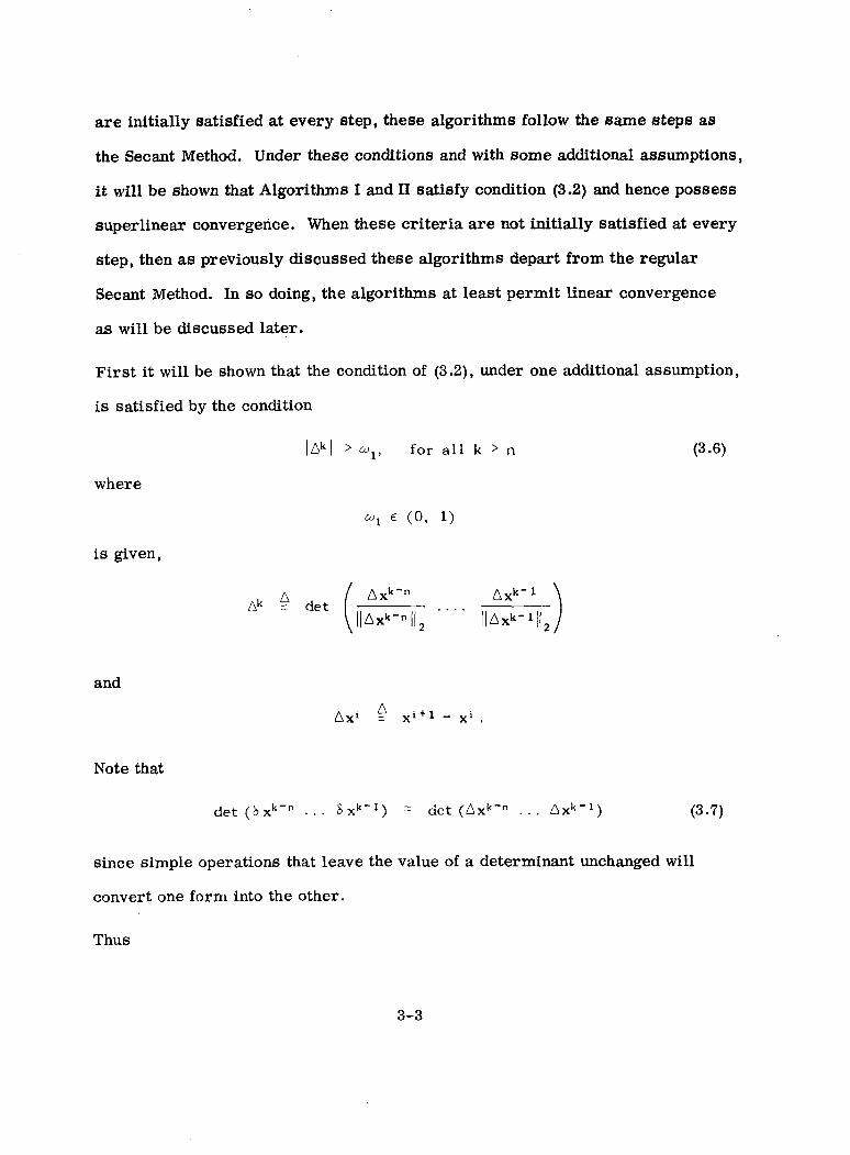
are initially satisfied at every step, these algorithms follow the same steps as

the Secant Method. Under these conditions and with some additional assumptions,

it will be shown that Algorithms I and I1 satisfy condition (3.2)and hence possess

superlinear convergence. When these criteria are not initially satisfied at every

step, then as previously discussed these algorithms depart from the regular

Secant Method. In so doing, the algorithms at least permit linear convergence

as will be discussed later.

First it wi l l be shown that the condition of (3.2), under one additional assumption,

is satisfied by the condition

where

is given,

and

A x i 4 x i + l - x i ,

Note that

det ( b xk-” . . . 8 xk-l) = det (Axk‘” . . . n x k - l ) (3.7)

since simple operations that leave the value of a determinant unchanged wi l l

convert one form into the other.

Thus

3-3

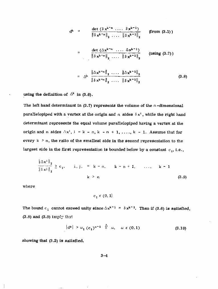
det ( 6 ~ ~ ' ".... 6xk")d k = II8 xk-nlI2 .. . . 11 s xk-'I12

(from (3.1))

-- det (Ax"-" .. . . Axk") (using (3.7))

llSxk-"Il2 . * . . lISxk-1lI2

using the definition of Ak in (3.6).

The left hand determinant in (3.7) represents the volume of the n-dimensional

parallelopiped with a vertex at the origin and n sides 6 x i , while the right hand

determinant represents the equal volume parallelopiped having a vertex at the

origin and n sides Ax', i = k - n, k - n + 1, ... ., k - 1. Assume that for

every k > n, the ratio of the smallest side in the second representation to the

largest side in the first representation is bounded below by a constant cl,i.e.,

where

c1 E (0,l l

The bound c 1 cannot exceed unity since Axk-' 6xk'l. Then if (3.6) is satisfied,

(3.8)and (3.9) imp!;. th3 t

AIdk[ > m1 (cl)n'1 = W , w E ( 0 , l ) (3.10)

showing that (3.2)is satisfied.

3-4

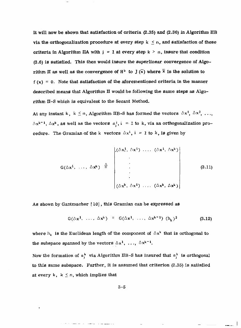
It will now be shown that satisfaction of criteria (2.35) and (2.36)in Algorithm IIB

via the orthogonalization procedure at every step k 5 n, and satisfaction of these

criteria in Algorithm IIA with j = 1 at every step k > n, insure that condition

(3.6) is satisfied. This then would insure the superlinear convergence of Algo­

rithm 11as well as the convergence of H k to J (x)where is the solution to

f (x ) = 0 . Note that satisfaction of the aforementioned criteria in the manner

described means that Algorithm II would be following the same steps as Algo­

rithm II-S which is equivalent to the Secant Method.

At any instant k , k 5 n , Algorithm IIB-S has formed the vectors Ax', Ax2, ..., A ~ k - 1 , AX^, as well as the vectors a / , i =. 1to k, via an orthogonalization pro­

cedure. The Gramian of the k vectors Ax' , i = 1 to k, is given by

( A x ? , Ax') . . . . ( A x ' , A x k )

(3.11)

A s shown by Gantmacher [lo],this Gramian can be expressed as

where h, is the Euclidean length of'the component of A x k that is orthogonal to

the subspace spanned by the vectors A x ' , ..., A xk- 1.

Now the formation of a,!' via Algorithm IIB-S has insured that a: is orthogonal

to this same subspace. Further, it is assumed that criterion (2.35) is satisfied

at every k, k 5 n , which implies that

3-5

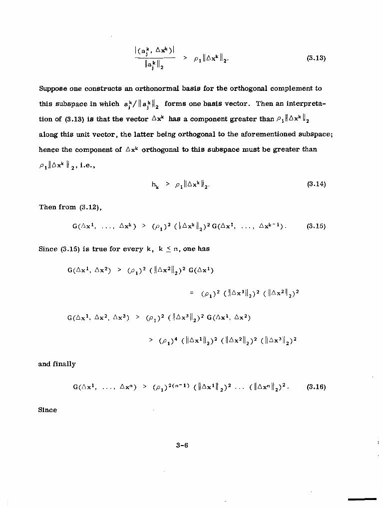
(3.13)

Suppose one constructs an orthonormal basis for the orthogonal complement to

this subspace in which a f / 11 af 11, forms one basis vector. Then an interpreta­

tion of (3.13) is that the vector Axk has a component greater than P i 11 Axk

along this unit vector, the latter being orthogonal to the aforementioned subspace;

hence the component of A x k orthogonal to this subspace must be greater than

p,IIAxk 11 2 , i.e.,

hk ' P l l l n X k l 1 2 . (3.14)

Then from (3.12),

G ( A x 1 , . . . , A x k ) > ( P , ) ~( IIAxk ( 1 2 ) 2 G ( A x ' , . . . , A x k - ' ) . (3.15)

Since (3.15)is true for every k, k 5 n , one has

and finally

~ ( A x 1 , . . . , AX.) > ( P ~ ) ~ ( " - ' )( IIAxlII 2 ) 2 . . ( I I A x " I I ~ ) ~ (3.16)

Since

3-6

(3.17)

equation (3.11) implies that

c(Axl, . . ., Axn) = det [ AX""]

= '[det ( A X n + l ) ] * . (3.18)

Hence from (3.16)and (3.18),

ldet (AXn' l )1 > (p1)" - ' 1lAx1l\ , . . . IlAxnI12 (3.19)

or

Thus criterion (3.7) is satisfied for k = n + 1. This result wil l now be extended

to all k, k > n .

Similar to (3.12),one can express G ( A x ~ ' - ~ + ...,A x k ) asl,

where h, is the length of the component of Axk that is orthogonal to the subspace

formed by the n - 1 vectors A x k - " + l , ..., Axk- * . Algorithm IIA-S forms a/

so as to be Orthogonal to this subspace; hence satisfaction of criterion (2.35)

produces the same inequality for h, as before, namely

3-7

II ~~ I I I I ,I.11, I 111 I I I I 1 I I 111111 11.11” 1 1 1 1 1 1 l . 1 ~ 1 1 1 1 1 1 1 1 1 . 1 I I I II II I1111

(3.22)

Hence,

2 G(Axk-n+l1 . . ., Ax,) > ( P , ) ~ (IlAxkI12) G(Axk’“+’, . . . ( Axk“). (3.23)

Now a:- ’,whether formed by Algorithm IIA-Sor IIB-S,is orthogonal to the

subspace formed by to Axka2 (it may be orthogonal to a larger subspace),

so that one obtains

2 .~ ( A X k - n + l , . . . ) Axk-1) > ( p 1 ) 2 (1lAxk-’II2) G ( ~ X ~ - ” + ~ , A x k e 2 ) . (3.24)

Continuing in this fashion,

2 .G ( b ~ k - ~ + l ,. . , Axk-2) > ( p l y (IlAxk-2Il2) G(nX“-n+l, , Axk-3)

(3.25)

Combining the above inequalities yields

2 G(Axk-n+l, . . . , AX”) > ( p 1 ) 2 ( n - V (JIAxk-n+l . . ( l l ~ x k l j 2 ). (3.26)

Since

(3.27)

one obtains

3-0

I

(3.28)

or

Ink\ > (p , ) ” - ’ 2 w l , k > n + 1. (3.29)

Combining (3.29) with (3.20) shows that condition (3.7) is satisfied for all k ,

k > n , when the criteria of Algorithms IIB and ILA are initially satisfied as de­

scribed. Then under these conditions and the previous assumptions, Algorithm I1

possesses local superlinear convergence of order at least that of the positive

root of (3.3).

The extension of these results to Algorithm I is fairly simple, although some

additional assumptions are required as wi l l be shown. First assume that cri­

terion (2.5) in Algorithm IB is satisfied at each step k 5 n via the orthogonaliza­

tion procedure and that this criterion in Algorithm IA is satisfied at each step

k > n by j = 1. Then in an analogous manner to the foregoing one obtains

det ( n f k - ” ~ -II A f k - n 1 1 2

. . . n f k - l )I > ( p , ) ” ” , k > n (3.30)IID fk’ 1 1 1 2

w.here p1 is a preselected number in the interval (0, 1). The matrices A X k and

AFk satisfy

3-9

AXk = H k A F k (3.31)

so that

det (AX") = det ( H k ) det ( O F k ) . (3.32)

Then from (3.32),

(using (3.30)and (3.31)). (3.33)

Assume that Hk is non-singular. This is not assured in Algorithm I even though

the satisfaction of criterian (2.5) assures the non-singularity of AF k. However,

as previously discussed, if the vectors A f comprising A F k are formed from

iterates close enough to a solution x,then the independence of the vectors A f

assures the independence of the corresponding vectors A x i (assuming J (X) is

non-singular) and hence assures the non-singularity of H k . Assume further that

(3.34)

where c 2 E (0,1].

Note that c cannot exceed unity since for any matrix A,

3-10

Ill

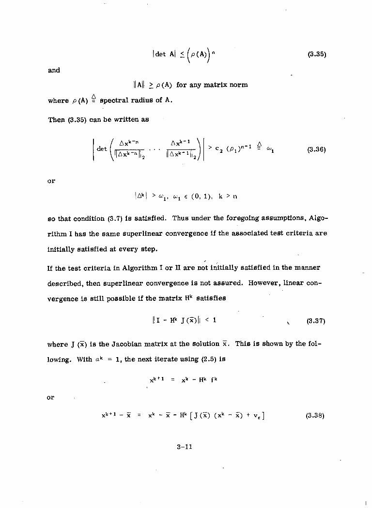
(3.35)

and

11 All p (A) for any matrix norm

where p (A) spectral radius of A.

Then (3.35) can be written as

(3.36)

or

lAkl > ul,w1 E (0,l) , k > n

so that condition (3.7)is satisfied. Thus under the foregoing assumptions, Algo­

rithm I has the same superlinear convergence if the associated test criteria a r e

initially satisfied at every step. I

If the test criteria in Algorithm I or 11are not iktially satisfied in the manner

described, then superlinear convergence is not assured. However, linear con­

vergence is still possible if the matrix Hk satisfies

where J (X) is the Jacobian matrix a t the solution X. This is shown by the fol­

lowing. With uk = 1,the next iterate using (2.5)is

X k + l = Xk - H k f k

(3.38)

3-11

-

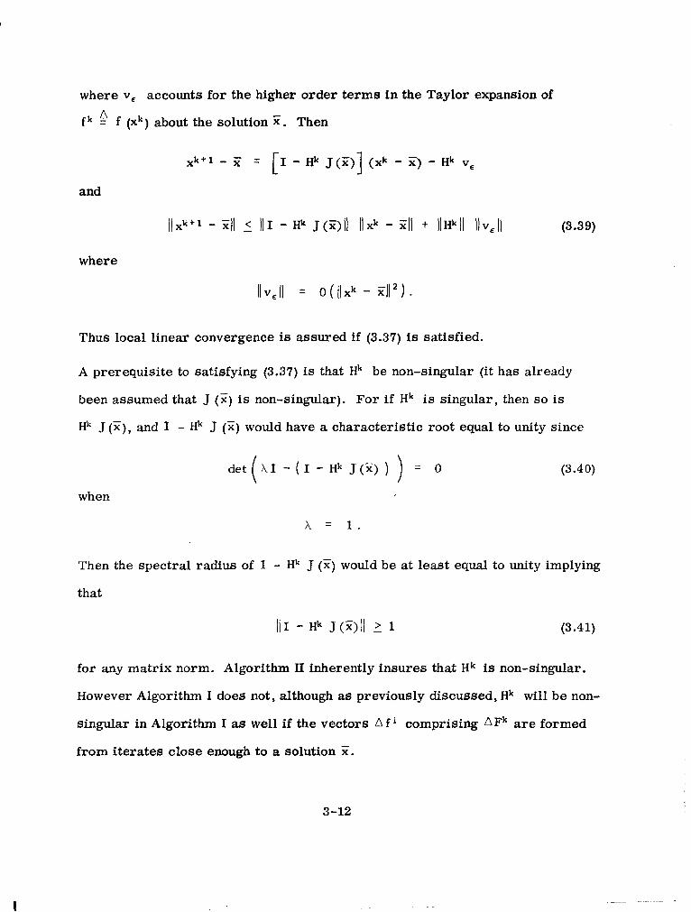
where v6 accounts for the higher order terms in the Taylor expansion of nf k = f (xk) about the solution E. Then

xk+l - X - [I - Hk J(Z)] (xk - -x) Hk vE

and

(3.39)

where

IIv,II = o ( IIXk - xl12)

Thus local linear convergence is assured if (3.37) is satisfied.

A prerequisite to satisfying (3.37) is that Hk be non-singular (it has already

been assumed that J (X)is non-singular). For i f Hk is singular, then so is

Hk J ( X ) , and I - Hk J (X)would have a characteristic root equal to unity since

when

A = 1 .

Then the spectral radius of I - Hk J (x)would be at least equal to unity implying

that

111 - Hk J(X)II 11 (3.41)

for any matrix norm. Algorithm IT inherently insures that H k is non-singular.

However Algorithm I does not, although as previously discussed, Hk wi l l be non­

singular in Algorithm I as well if the vectors A f comprising nFk are formed

from iterates close enough to a solution X.

3-12

Even though Hk is non-singular in Algorithm 11, and assumed to be so in Algo­

rithm I, there still is no assurance that (3.37)will be satisfied. Heuristically

though, one would expect this to be the case if for example the initial estimate H1

is a good approximation to J (51) and if the problem is not severely nonlinear. In

any event, the conditions under which Algorithms I and 11depart from the Secant

Method are those tending to cause poor convergence of the latter. The alterna­

tives followed by Algorithms I and I1 in these circumstances at least retain the

potential for linear convergence .

3-13

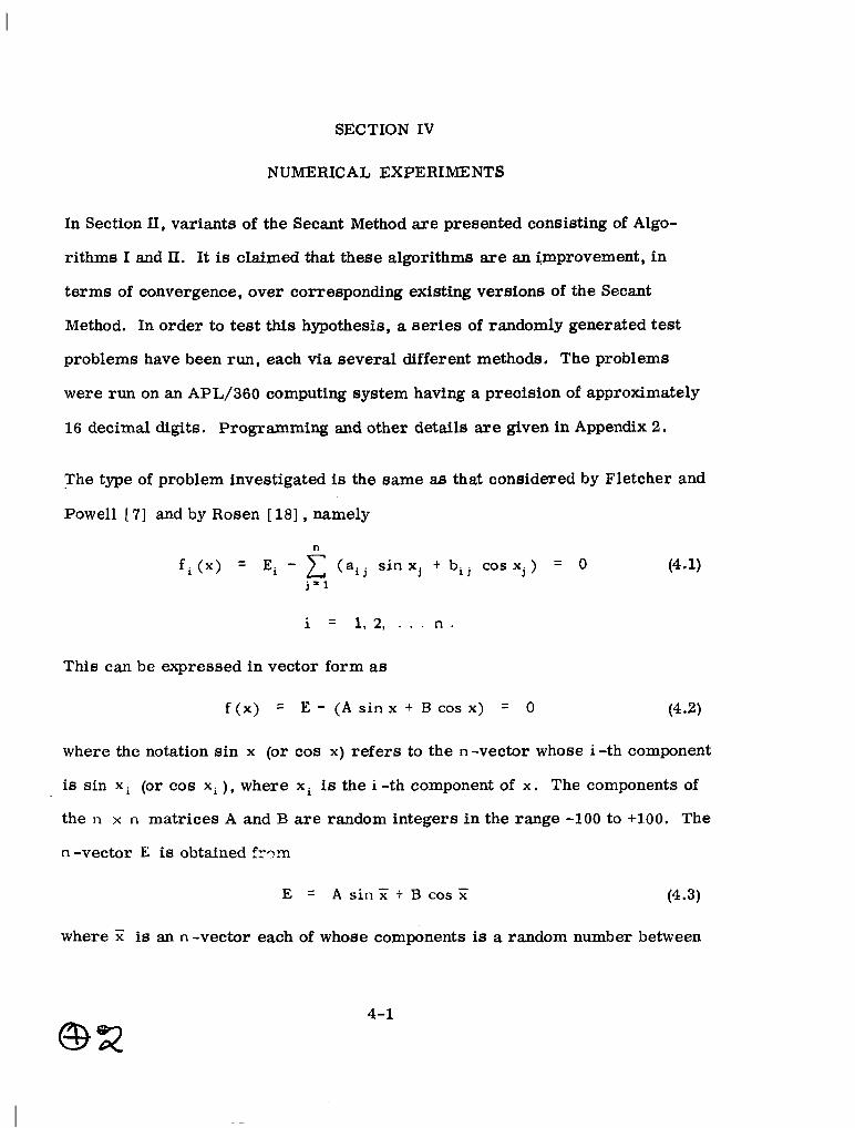
SECTION IV

NUMERICAL EXPERIMENTS

In Section 11, variants o the Secant Method are presenteG consisting of Algo­

rithms I and 11. It is claimed that these algorithms are an improvement, in

terms of convergence, over corresponding existing versions of the Secant

Method. In order to test th is hypothesis, a series of randomly generated test

problems have been run, each via several different methods. The problems

were run on an APL/360 computing system having a precision of approximately

16 decimal digits. Programming and other details are given in Appendix 2.

The type of problem investigated is the same as that considered by Fletcher and

Powell [ 71 and by Rosen [ 181 , namely

n

f i ( x ) = Ei - ( a i j s i n x j t b i j cosx j ) = 0 j = l

i = 1 , 2 , . . . n

This can be expressed in vector form as

f ( x ) = E - ( A s i n x f B COS x) = 0 (44

where the notation sin x (or cos x) refers to the n -vector whose i -th component

i s sin x i (or cos xi ), where x i is the i -th component of x. The components of

the n x n matrices A and B a r e random integers in the range -100 to +loo. The

n-vector E is obtained f x m

E = A s i n X + B cos Ti: (4.3)

where X is an n-vector each of whose components is a random number between

4-1

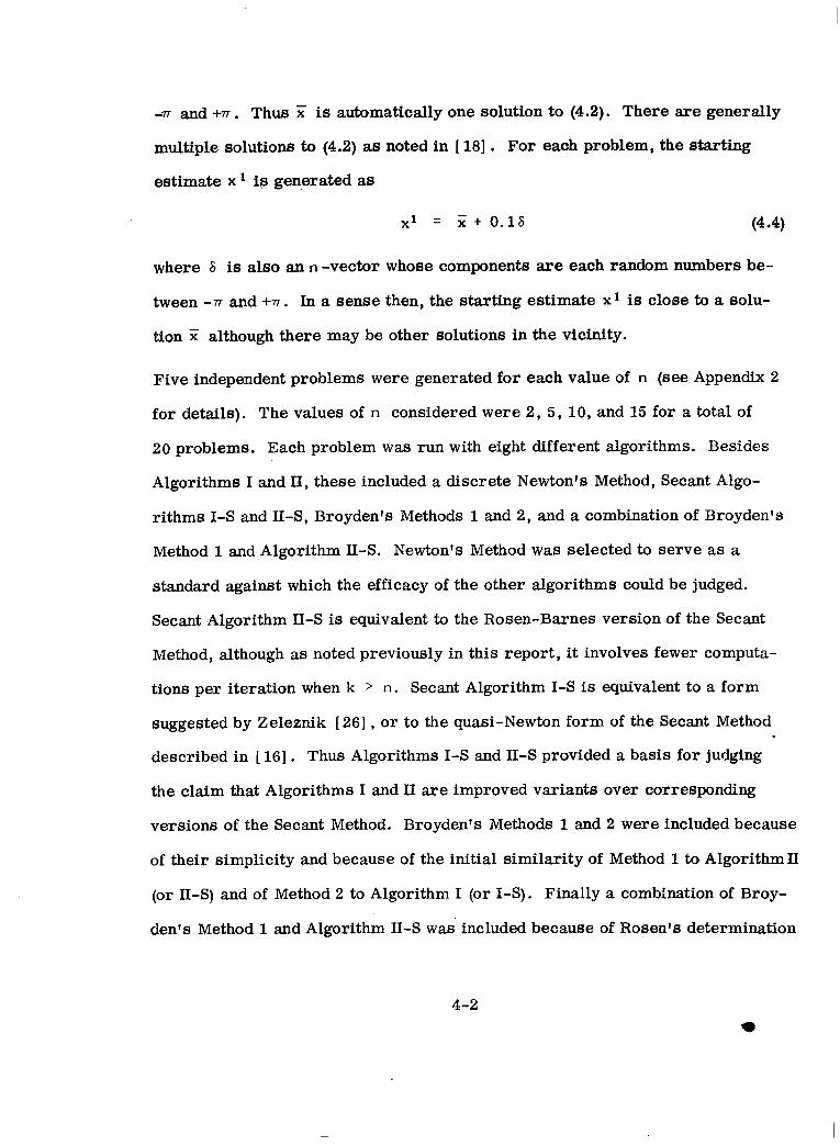
-n and +n . Thus X is automatically one solution to (4.2). There are generally

multiple solutions to (4.2) as noted in [ 181 . For each problem, the starting

estimate x is generated as

where 6 is also an n -vector whose components are each random numbers be­

tween -n and +n. In a sense then, the starting estimate x l is close to a solu­

tion X although there may be other solutions in the vicinity.

Five independent problems were generated for each value of n (see Appendix 2

for details). The values of n considered were 2, 5, 10,and 15 for a total of

20 problems. Each problem w a s run with eight different algorithms. Besides

Algorithms I and II, these included a discrete Newton's Method, Secant Algo­

rithms I-S and 11-S, Broyden's Methods l and 2, and a combination of Broyden's

Method 1 and Algorithm II-S. Newton's Method w a s selected to serve as a

standard against which the efficacy of the other algorithms could be judged.

Secant Algorithm 11-S is equivalent to the Rosen-Barnes version of the Secant

Method, although as noted previously in this report, it involves fewer computa­

tions per iteration when k > n. Secant Algorithm I-S is equivalent to a form

suggested by Zeleznik [26],or to the quasi-Newton form of the Secant Method

described in [ 161. Thus Algorithms I-S and 11-S provided a basis for judging

the claim that Algorithms I and 11 are improved variants over corresponding

versions of the Secant Method. Broyden's Methods 1 and 2 w e r e included because

of their simplicity and because of the initial similarity of Method 1 to AlgorithmII

(or 11-S) and of Method 2 to Algorithm I (or I-S). Finally a combination of Broy­

den's Method 1 and Algorithm 11-S was included because of Rosen's determination

4-2

that such a combination generally yielded better results in his series of

problems than either method alone.

When Algorithm I o r 11w a s utilized, it w a s necessary to specify a value of p l .

Each time these Algorithms were employed, two o r more runs were made with

different values of p 1, in order to obtain some measure of the effect of p on

convergence. Concurrently, an attempt was made to develop a rule of thumb for

selecting a nominal value of P that would yield good results. Section 111pro­

vided some insight on the effect that p1 has in establishing a lower bound for

the ill-conditioning of Axk. This together with initial experimentation resulted

in the selection of some "nominal" values of p1 as n x and 2n x lo'? The

results using these values of p1 are listed in subsequent tables.

When Algorithm I1 w a s used, it w a s also necessary to specify a value of p2 . In

order to avoid a further increase in the number of runs, which was already con­

siderable, only one value of p 2 was specified for each value of p 1. The specifica­

tion w a s arbitrarily set at p , = 0.1 p 1 . The parameter p 2 is used in criterion

(2.36) to insure the independence of the vectors A f that are retained for subse­

quent use. However when mk < n , criterion (2.36) is a sufficient but not neces­

sary condition for assuring this independence. In other words, criterion (2.36)

could fa i l even though the vectors A f were sufficiently independent. In order

to reduce the probability of this unnecessary rejection of a; as formed by

orthogonalization, it w a s deemed desirable to set p2 lower than p l . At the same

time a value of p2 > 0 w a b &ill considered necessary to avoid )lHk11 -, a.

In the combination of Broyden's Method 1and Algorithm II-S,the vector zk in

4-3

H k + l = Hk + (Axk - Hk A f k ) (zk>' Hk

(zk)= Hk A f k (4.5)

is formed a8 =,average of'the vectors in the individual methods. When each of

the above methods is used by itself, only the direction of zk is important since,

a constant multiplier has no effect. But when an average of 60different vectors

is performed, the relative scaling assigned to each is important since it affects

the direction of the resultant average. Since this scaling was not explicitly de­

scribed in Rosen's paper [ 181 ,the author decided on the magnitude scaling in­

herent in each method as it is described elsewhere in this report. Thus in

Broyden's Method 1, zk is set equal to Axk, while in Algorithml-S Zk is the

component of Axk that is orthogonal to the subspace formed by the previous

vectors A x i , 0 < k - i < n . In this scheme, the ratio of the magnitude of zk as

produced by Algorithm 11-S to that produced by Broyden's Method 1is a maximum

of unity when A x k is orthogonal to the aforementioned subspace and becomes zero

when Axk lies in this subspace.

All of the algorithms that have been listed could be utilized either in a full step

version (ak = 1)or in a reduced-step version (ak selected to minimize o r reduce

v k + l ) . Only the full step version w a s used in these experiments for the following

reasons. Methods that select ak on the basis of minimizing are somewhat

inefficient in terms of function evaluations. Secondly, there are a great many norm-

reducing schemes. To utilize even just a few of these on top of the run permuta­

tions already considered would result in a morass of data in which the basic pur­

pose of the investigations would be masked. Certainly the relative efficiency of ' norm-reducing methods is peripheral to this investigation. The basic purpose of

this experimentation is to test the convergence characteristics of Algorithms I

4-4

and II near a solution and to compare them with those of Secant Algorithms I-S

and 11-S among others. This comparison is facilitated by the use of a single gen­

erally accepted method of selecting the step size and certainly ak = 1qualifies.

-Each algorithm considered requires an initial estimate H1 of the inverse Jacobian

as well as an initial estimate x1 of the solution. Algorithms I and II, as wel l as

I-S and IC-S, could function with any initial estimate H provided a norm-reducing

method for selecting the step size were included. These algorithms, for a linear

system, generate the system inverse Jacobian after at most n iterations. For a

non-linear system, these algorithms would generate an approximation to the in­

verse Jacobian at x1 within n iterations, provided the step size were not so

great as to drive the iterate to a locale with a markedly different Jacobian. A

norm-reducing constraint would generally prevent such deviations. However,

norm-reducing schemes were not included in this numerical experimentation for

reasons previously discussed. Secondly, 'starting with an arbitrary H' (e.g.,

H' = I) provides little if any saving in computations since the n iterations re­

quired to develop a good approximation to the inverse Jacobian at x 1 are com­

parable to the computational effort in directly calculating an approximate J' l(x).

For these reasons, the initial estimate H in this investigation w a s uniformly

generated by computing a discretized approximation to J (x') and obtaining its

inverse. This selection also has the effect of not penalizing Broyden's Method

unnecessarily; the latter is at its best when H' % J-'(xl).

The use of the full-step T w - P i m for all of the algorithms, as opposed to a reduced-

step norm-reducing version, raises the possibility that in some cases the iteration

wil l fail to converge to a solution for any of the methods. To accommodate this

possibility the following strategy w a s adopted. If all of the quasi-Newton

4-5

algorithms (i.e., all except the discrete Newton's Method) failed to converge to

a solution, the starting estimate x1 given by (4.4) would be changed to

x1 = x t (+)q x 0.18

where q assumed the values 1,2, etc., until at least one of the quasi-Newton

methods converged to a solution.

The effect of (4.6) is to bring the starting estimate x1 closer and closer to a

solution X so as to increase the probability of convergence. The reason for

adopting this strategy is that the main purpose of the investigation is to compare

the local convergence of Algorithms I and 11with that of the other quasi-Newton

methods, especially that of Secant Algorithms I-S and 11-S. The latter methods

will at times encounter difficulties after reaching points very close to a solution;

it is primarily this type of problem that Algorithms I and 11 were designed to

overcome. An evaluation of the region of convergence of the various methods is

beyond the scope of this investigation. In the actual numerical work, equation (4.6)

had to be utilized only once, in problem 55, when all of the quasi-Newton methods

failed to converge. The use of q = 1in (4.6) resulted in all of the methods con­

verging to a solution in this problem.

In judging the effectiveness of the various algorithms in this particular series of

problems, the primary criterion used is the number of vector function evaluations

required by the algorithm to converge to a solution. This criterion, which has

been used by many authors, is simple to apply and provides a'fair representation

of total computational effort especially if the function is at all complicated. In

the discrete Newton's Method, n + 1function evaluations are required at each

step except the last, where only one evaluation is required. The other

4-6

(quasi-Newton) methods require but one function evaluation per step except for

the first step (k = 1) which requires n + 1 evaluations to establish the initial

estimate H l . Thus denoting the final iterate index as k , (at which rpkf is less

than the convergence criterion), the total number of function evaluations is

. givenby

No. of f evaluations = &, - 1) (n + 1) + 1 (4.7)

= k , (n + 1) - n

for the discrete Newton's Method, and by

=No. of f evaluations &f - 1) f (n f 1)

for the quasi-Newton methods. The convergence criterion in all cases was

arbitrarily set at

o r

A secondary criterion used to judge the effectiveness of the various algorithms

is the accuracy of the final matrix Hkf generated by each algorithm, since the

accuracy of the estimated inverse Jacobian at the solution is of importance in

some applications. Also the accuracy of Hkfis a distinguishing characteristic,

especially in those cases where convergence is poor. The standard used for

comparison is the inverse of the estimated Jacobian at the solution as determined

by the same discrete process used in the discrete Newton'B Method. Denoting the

4-7

latter matrix as J' (F),the e r ror criterion used is the maximum absolute

component value of the e r ror matrix (Hkf - J-' (Z) ).

For purposes of comparison, it is convenient to divide the quasi-Newton algo­

rithms into two groups. Group 1 consists of those algorithms in which the up­

dating of Hk has the form

HkH k t l = Hk +- (Axk - Hk A f k ) ( z ~ ) ~ (4.10)

( ~ k ) ~ A fkHk

This group then includes the Broyden 1 algorithm, Algorithms II and 11-S,and

the combination of Broyden 1 and Algorithm 11-S. Similarly, Group 2 algorithms

are classified by the form

H k + l = Hk .+ (Axk - Hk A f k ) ( z k ) = (4.11)

( z " ) ~A f k

Group 2 then consists of the Broyden 2 algorithm and Algorithms I and I-S.

The results of the computer runs in this series of problems are summarized in

Tables 4.1 through 4.4. When convergence occurred, as determined by 11 f / I 2 < 10-6,

the distance of the final iterate xkf from a true solution was always less than 10'6

(as measured in the infinity norm). Usually, the closeness of xk* to a true solu­

tion w a s in the order of An asterisk next to the number of function evalua­

tions for convergence indicates convergence to a solution other than the nominal

solution X originally set up. In all cases, these other solutions were within 27-1

of X and usually much closer. The term I1Divergeffis used to indicate when an

algorithm w a s divergent, the criterion being divergence to a distance (again in

the infinity norm) of 100 o r more from 51. The term l.'Oscllis used to denote

4-8

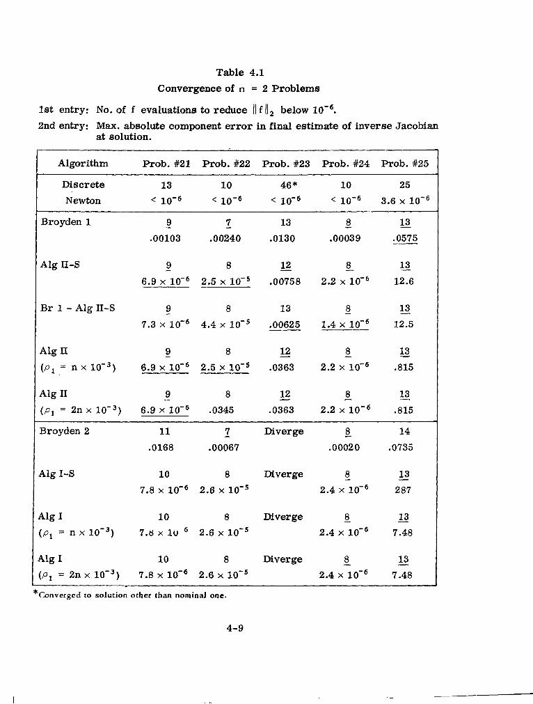
Table 4.1

Convergence of n = 2 Problems

1st entry: No. of f evaluations to reduce 11 f / I 2 below 2nd entry: Max.absolute component e r ro r in final estimate of inverse Jacobian

at solution.

Algorithm mob. #21 Prob. #22 Prob. #23 R o b . #24 Prob. #25 ~~

Discrete 13 10 46* 10 25 Newton < 10-6 < 10- < 10-j < 3.6 x

Broyden 1 -9 -7 13 -8 13 .00103 .00240 .0130 ,00039 .0575-~

- -8 13Alg II-S -9 8 12 6.9 x 2.5 x lo-’ .00758 2.2 x 10- 12.6

B r 1 - Alg II-S 9I 8 13 -8 13 7.3 x 4.4 x ,00625 1.4 x 12.5

- -A l g II -9 8 12 -8 13

( p l = n x 6.9 x 2.5 x .0363 2.2 x 10-6 .815

Alg I1 -9 8 12 -8 13­-( p l = 2n x 6.9 x .0345 .0363 2.2 x 10-6 .815

~ ~~ ~~~ ~~~ ~~

Broyden 2 11 -7 Diverge -8 14 .0168 .00067 .00020 .0735

4lg I-S 10 8 7.8 x 2.6 x lo-’

Diverge -8 2.4 x

-13 287

llg I 10 8 :pl = n x 7.8 x 10 2.6 x lo-’

Diverge s 2.4 x

-13 7.48

ilg I 10 8 ‘p l = 2n x 7.8 x loe6 2.6 x

Diverge -8 2.4 x

-13 7.48

*Converged to solution other than nominal one.

4-9

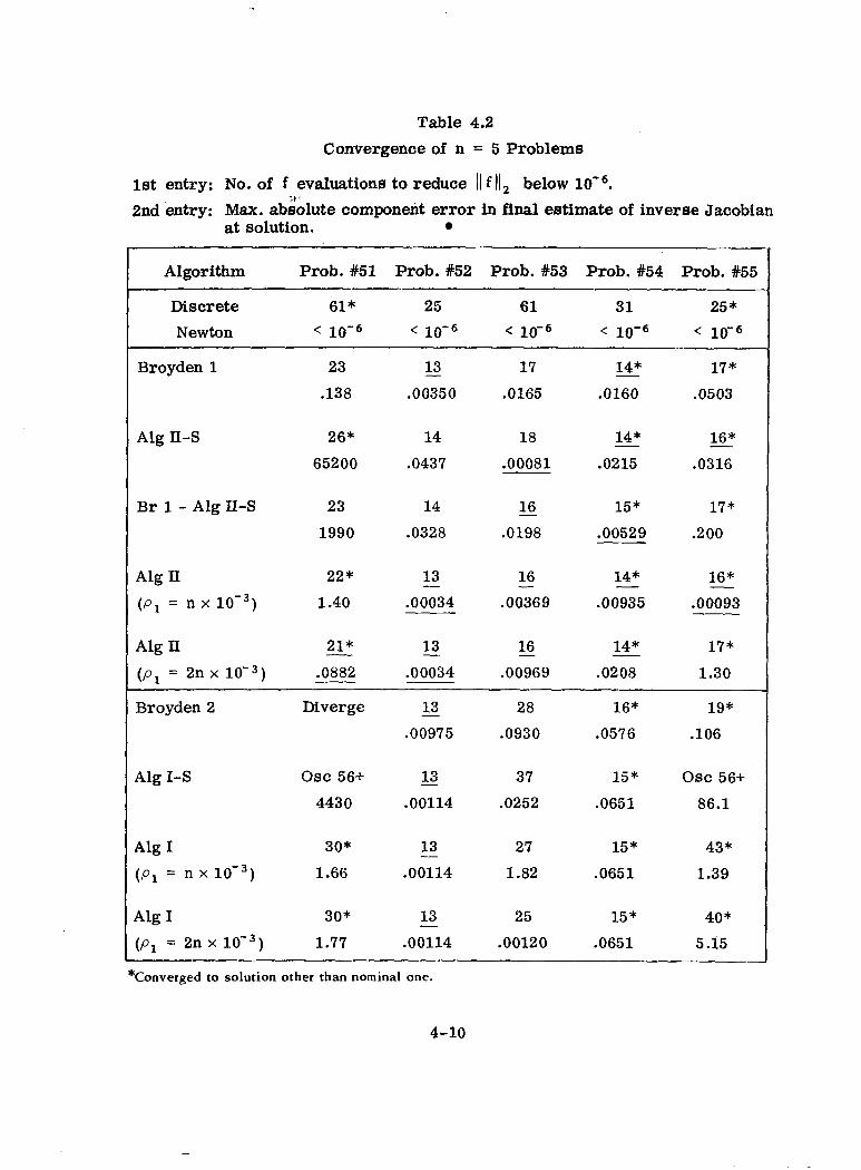
Table 4.2 Convergence of n = 5 Problems

1st entry: No. of f evaluations to reduce 11 f 11, below 3 '

2nd entry: Max. absolute component error in final estimate of inverse Jacobian at solution.

Algorithm

Discrete Newton

Broyden 1

Alg 11-S

Br 1 - Alg II-S

Alg II ( p l = n x

Alg 11 ( p l = 2n x 10-3)

Broyden 2

Alg I-S

Alg I ( p l = n x

Alg I ( p l = 2n x

Prob.#51 Prob. #52 Prob. #53 Prob. #54 Prob. #55

61* 25 61 31 25* < 10-6 < < 10-6 < 10-6

~~

23 13- 17 14* 17*-.138 .00350 ,0165 .0160 .0503

26* 14 18 14* 16*- ­65200 .0437 .00081 .0215 .0316

23 14 16 15* 17*-1990 .0328 .0198 .00529 .200-22* 13 16 14* 16*- - - ­1.40 .00034 ,00369 .00935 ,00093

21*- 13- 16- 14*- 17* .0882 .00034 .00969 .0208 1.30

Diverge 13- 28 16* 19* .00975 .0930 .0576 .lo6

Osc 56+ 13- 37 15* Osc 56+ 4430 ,00114 .0252 .0651 86.1

30* 13 27 15* 43* -1.66 .00114 1.82 .0651 1.39

30* 13 25 15* 40*-1.77 .00114 .00120 .0651 5.15

*Converged to solution other than nominal one.

4-10

Table 4.3 Convergence of n = 10 Problems

1st entry: No. of f evaluations to reduce 11 f below 2nd entry; Max. absolute component e r ror in final estimate of inverse Jacobian

at solution. .

Algorithm Prob. #lo1 Prob. #lo2 Prob. #lo3 Prob. #lo4 Prob. #lo5 .__ - . . - ._.

Discrete 45 Diverge 45 89* 56 Newton 10-6 < 10-6 1.2 x 10-6 < 10-6

-. ~ ~. -~ .. .

Broyden 1

Alg 11-S

Br 1- Alg 11-S

Alg 11 ( p l = n x

Alg 11 (p l = 2 n x 10-3)

_.

Broyden 2

41g I-s

91g I [p l = n x

21 36- 22 27* 24 .00963 .169 .00235 1.37 .00682-

21 94 - 31* 23 .00489 30.9 .00348 259 .0192

21 62 22 29* 24 .00928 10.2 .00867 294 2.09

21

26"20 37 -21 - 22-.00163 2.07 .00348 .147- ,0215

20- 40 -21 26* 23 .00163 .284 .00360 ,152 .0371

23 Diverge 23 31* 26 .0105 .00470 .231 .0436

21 .0791 .00355 83.2 .410

21 Diverge -21 28* 27 .ui51 .00355 3.77 .437

21 Diverge -

21 Diverge - 29* 28

21 28* 27 .00547 .002 13 2.51 .414

. .

*Converged to solution other than nominal one .

4-11

- -

Table 4.4 Convergence of n = 15 Problems

1st entry: No.'of f evaluations to reduce 11 f 11, below 2nd entry: Max. absolute component error in final estimate of inverse Jacobian

at solution. .. .. . - - . . . ..

Algorithm Prob. #151 Prob. #152 Prob. #153 Prob. #154 Prob. #15f - _ _ -

Discrete 81 129* Diverge 161 97 Newton 10-6 < 10-6 < 10-6 < 10-6

- -~ -

Broyden 1

Alg II-S

Br 1 - Alg II-S

Alg Is (pi = n x 10-3)

Alg II ( p l = 2n x

Broyden 2

Alg I-S

AIg I

( p l = n x

__I..

-28 Diverge 35 36* 31 .00449 .0153 .366 .0127

28 33 30- osc 91+ - 34 ­

.0193 1.55 .157 2.64 .0719

28 30- Diverge 36 35 ­

.00!23 .116 406 ,00996

28 51* -33 32 30- - ­.0193 .538- .0313 .133 .0289

-28 41* 33 -32 ­- 30 .00584 1.19 .0262 .118 .00922

~ - . .

32 Diverge Diverge 35 32 .0300 .846 .0330

30 osc 91+ 61* 34 31 .152 2.70 11.2 12.5 .155

30 osc 91+ 63 34 31 .0272 .595 .411 2.08 .152

31 56* 106* 34 31 .0285 1.74 .753 1.58 .211

_ _ _ -

*Converged to solution other than nominal one.

4-12

convergence to the vicinity of a solution but lack of convergence to a solution

within the stated (large) number of function evaluations.

For each problem, the algorithm(s) providing convergence with the least number

of function evaluations is (are) identified by the underlining of this number.

Similarly, the quasi-Newton algorithm(s) yielding the smallest component error

in Hkf is (are)identified by the underlining of this error . In many problems

more than one algorithm provided convergence with the minimum number of

evaluations. On occasion, more than one quasi-Newton algorithm yielded both

the minimum number of evaluations and the minimum component e r ror in Hkf . When this occurred, o r when more than one algorithm yielded the same two

numbers regardless of whether they were minima or not, the reason w a s that

these algorithms were following exactly the same path. Thus for example in

Problem #21, both cases of Algorithms I1 as well as Algorithm II-S followed

identical paths since the cri teria associated with Algorithm II were initially

satisfied at every step. In Problem #52, both cases of Algorithm I1 happened to

follow the same step-by-step procedure (but not the same as in Algorithm 11-S)

even though the associated p1 criteria differed by a factor of two.

The algorithms in Tables 4.1 through 4.4 are arranged in the order of discrete

Newton's Method, then Group 1 algorithms and lastly Group 2 algorithms. A

quick perusal of these tables reveals that the discrete Newton w a s generally the

least efficient in terms of function evaluations. This w a s pretty much expected

in view of the required n + 1function evaluations per iteration. The discrete

Newton converged to a solution in every problem except two (Problems #lo2

and #153). That divergence occurred twice is not surprising. The multiplicity

4-13

of roots in a small region implies that the Jacobian is singular at many points

in this region. A chance landing close to one of these points could throw the

next iterate f a r out with no chance of recovery. This apparently occurred in

Problems #lo2 and #153. When convergence occurred, the discrete Newton

always provided the most accurate estimate of Hkf (generally within of

J (X)), as would be expected.

A further perusal of these tables reveals that as a group, the Group 1 algorithms

were generally more effective than Group 2, this behavior becoming more pro­

nounced as n increased. Moreover this is the case in an algorithm by algorithm

comparison of corresponding algorithms in each group. Thus Broyden 1w a s

generally more effective than Broyden 2,Algorithm 11 more effective than Algo­

rithm I, and Algorithm 11-S more effective than Algorithm I-S. In the case of

Broyden 1and Algorithm 11, their greater effectiveness (over the corresponding

versions in Group 2) may be due in part to their inherently avoiding H k becoming

singular, as previously shown in this report. In the case of Algorithm 11-S vs.

I-S, neither algorithm insures against the singularity of Hk . However when k < n ,

Hk is less likely to become singular in Algorithm 11-S than in I-S. This is shown

by the following.

Assume that Hk is non-singular. Then as shown in Section I , H k + l in Algo­

rithm 11-S wi l l become singular (for A x k # 0) if and only if

( z k ) T A x k = 0 . (4.12)

This occurs only when Axk lies in the subspace of the previous vectors AX',

0 < k - i < n . In the case of Algorithm I-S, a similar development shows

that H k + l becomes singular (for Axk # 0) if and only if

4-14

( z k ) T Jk Axk = 0 . (4.13)

Recall that in Algorithm I-S, z k is formed to be orthogonal to the previous

vectors A f i , 0 < k - i < n ,o r

( z k ) T A f i = 0, 0 < k - i < n . (4.14)

But A f satisfies

(4.15)

which when substituted in (4..14)yields

Jk( z ~ ) ~A x i = 0 , 0 < k - i < n .

Thus the vector (Jk)T zk in Algorithm I-S is always orthogonal to the vectors A x ' ,

0 < k - i < n . If A x k lies in the subspace formed by these vectors, then (Jk)>' z k

must be orthogonal to A x k as well , showing that (4.13)holds. In addition, when

k < n , it is possible for the vector (Jk)T zk to be orthogonal to A x k even if the

latter lies outside the aforementioned subspace since this subspace would be of

dimension less than n - 1. If one assumes that the vectors Axk in both algorithms

are more o r less randomly oriented, then there is greater likelihood of Hk be­

coming singular in Algorithm I-S than in 11-S. This may be a factor in the better

performance of Algorithm 11-S compared to Algorithm I-S.

To facilitate the comparison of performance of algorithms within a group,

Tables 4.5 and 4.6 have been prepared. For each set of problems, these tables

list the number of times an algorithm reached convergence in the fewest evalua­

tions, the number of times an algorithm yielded the most accurate matrix Hkf ,

and the number of times the algorithm failed to converge. The first two

4-15

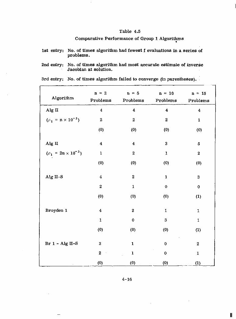
Table 4.5

Comparative Performance of Group 1 Algorithms c

1st entry: No. of times algorithm had fewest f evaluations in a series of problems.

2nd entry: No. of times algorithm had most accurate estimate of inverse Jacobian at solution.

3rd entry: No. of times algorithm failed to converge (in parentheses).

n = 2 n = 5 n = 10 n = 15 Algorithm Problems Problems Problems Problems

Alg I1

( p l = n x

Alg I1

( p l = 2nx

Alg 11-S

Broyden 1

Br 1- Alg 11-S

Table 4.6

Comparative Performance of Group 2 Algorithms

1st entry: No. of times algorithm had fewest f evaluations in a series of problems.

2nd entry: No. of times algorithm had most accurate estimate of inverse Jacobian at solution.

3rd entry: No. of times algorithm failed to converge (in parentheses).

Algorithm

Alg I

( p l = n x

Alg I

( p l = 2n x

Alg I-S

Broyden 2

n = 2 n = 5 Problems Problems

3

3

(1)

3

3

(1)

2

-

n = 10 n = 15

Problems Problems - __­

3 3

0 2

(1) (1)

4-17

I

I

comparison numbers are based on the best performance in each problem of the

algorithms in the group rather than of all algorithms tested.

Table 4.5 reveals that' either case of Algorithm 11was generally more effective

than any of the other algorithms in the group. Besides yielding the fewest function

evaluations in general, Algorithm II converged in all of the 20 random problems

under test whereas the other algorithms in the group each failed to converge

once (in Problem #152). In addition, the convergence of Algorithm II-S w a s very

poor in one other problem (Problem #102) where it required 94 evaluations to

reach a solution. The combination of Broyden 1 and Algorithm II-S did not per­

form any better on the average than the individual algorithms comprising it. In

the aforementioned problem (#102) when Algorithm II-S had poor convergence,

this combination did much better than Algorithm II-S but still much worse than

Broyden 1. It would seem that Broyden 1is to be preferred over this combina­

tion algorithm.

Table 4.6 reveals that Algorithm I with p 1 = 2n x w a s generally more

effective than any of the other algorithms in the group. Although it failed to

converge twice (in Problems #23 and #102),none of the other algorithms in the

group converged in these two problems. In addition, Algorithm I-S and Broyden 2

failed to converge three additional times. Algorithm I with p1 = n x w a s

not quite as effective as with p1 = 2n x although it still.performed better

on the average than either Algorithm I-S o r Broyden 2. Both cases of Algorithm I

generally yielded smaller e r ro r s in H k f than did Algorithm I-S. In addition

Algorithm I-S often had some strikingly large e r ro r s in Hkf even when it con­

verged (see tabulation for Problems #25, #104, #153, and #154). Broyden 2,

4-18

when it converged, yielded a fairly accurate Hkf ,almost as good on the average

as did Algorithm I.

It is of interest to examine the cases where Algorithm I-S o r 11-S converged to

a region near a solution but failed to converge to a solution (denoted by TTOscll

in Tables 4.1 through 4.4), and also those cases where either of these algorithms

required an excessively large number of evaluations to reach a solution. In

problem #51,Algorithm I-S reached the vicinity of a solution within about 25

function evaluations but oscillated erratically thereafter. When terminated, the

e r ror in (Hk- J- (TI) ) for either of the known solutions in the vicinity was an

astounding 4430. This number also approximated the magnitude of the largest

component of Hk since the components of J' (X) were less than one in all of

the problems. At the same time, the determinant of Hk measured only -1.3 x

indicating a poorly conditioned, near singular matrix. The relative independence

of the vectors Axi comprising the matrix AXk, as measured by program COND

described in Appendix 2, w a s only 6.0 x 10-l3. Thus the poor conditioning of this

set of vectors w a s apparently the major factor in causing an erroneous, near-

singular matrix H k ,and in preventing convergence.

In problem #102,Algorithm 11-S required 94 function evaluations to reach the

expected solution, with the e r ror in H k f being quite large (30.9). Again Hkf was

near singular (det H k f = 7.8 x and the conditioning of the vectors Axi

comprising A X k f was extremely poor (6.0 x Periodic measurements

during this run of the e r ror in Hk, the determinant of Hk ,and the conditioning

of A X k showed the same pattern. This same pattern w a s also in evidence in

Problem #55 where Algorithm I-S exhibited continual oscillatory behavior in the

vicinity of a solution, and in Problem #152 where Algorithms I-S and 11-S both

4-19

exhibited erratic oscillation in the vicinity of a solution and failure to converge.

Thus the inability of Algorithms I-S and II-S to prevent near singular matrices

Hk appears to be a factor in delaying o r preventing convergence at times.

Algorithm I exhibited a related type of behavior in two cases, Problems #152

and #153. In Problem #152, Algorithm I with p1 = n x loe3.failed to converge

after 91 function evaluations although it w a s close to a solution. However its

behavior near the solution w a s not at all erratic and the iteration would have

undoubtedly converged to a solution if the run had not been terminated. There

had been no change in Hk and D: for about 25 iterations preceding termination

since A fk at each of these steps was insufficiently independent of any set of

(mk - 1)of the previous vectors A f retained in D:. The value of 11 fk w a s

geometrically decreasing with a ratio of between .91 and .94 over these 25 itera­

tions indicating (slow) linear convergence. The unchanging matrix Hk was near

singular and the conditioning of the vectors Axi corresponding to the aforemen­

tioned A f w a s very poor. This situation is not altogether unexpected since only

the independence of the vectors A f retained in D: is assured in Algorithm I.

A s noted in Chapter 111, the independence of the corresponding vectors Axi would

be assured only if these vectors had been formed from iterates sufficiently close

to the solution. This apparently was not the case in this particular problem.

In Problem #153 with p = 2n x a similar situation occurred although here

the iteration w a s allowed to continue to a solution (in 106 evaluations) because

the linear rate of convergence w a s better (about 0.76). This rate of convergence

existed over the 50 iterations preceding convergence, during which time Hk and

DF (= AI?) w a s retained unchanged for the same reason as before. Again the

matrix Hk was near singular and the conditioning of the vectors A x i , corresponding

4-20

to the vectors A f i retained in ll:, w a s very poor. Despite these two cases of

very slow convergence, Algorithm I on the average showed better performance

than Secant Algorithm I-S, both in the number of evaluations required for con­

vergence and in the accuracy of Hk'. A number of runs were made with Algorithms I and 11in which the value of pr

w a s either much larger o r much smaller than the %ominal" values of n x

and 2n x 10-3 . Sometimes these runs produced better results than for the

"nominal1' values of p l . More often, the results w e r e not quite as good. In

general, too small a value of pl simply resulted in Algorithms I and II degen­

erating into Algorithms I-S and 11-S respectively. Too large a value of p1 often

delayed or prevented convergence. No thorough attempt w a s made to optimize

the selection of p l . The rule of thumb developed for selecting Tfnominalllvalues

of p1 proved adequate to demonstrate improved performance of Algorithm I

over I-S and of Algorithm I1 over 11-S in this ser ies of problems. While the

results from this one series of problems are not conclusive, these results do

support the claim that Algorithms I and II are improvements over Secant Algo­

rithms I-S and 11-S respectively.

As noted earlier, Algorithm 11 showed better performance than did Algorithm I.

This w a s true in almost every problem, in terms of ability to converge, the

number of function evaluations required, and the accuracy of H k f . A s discussed

earlier, this is attributed in large measure to the inherent ability of Algorithm I1

to avoid singular o r near singular matrices Hk,which is lacking in Algorithm I.

This characteristic is directly associated in Algorithm 11with the selection and

retention of t".fficiently'l independent vectors Ax' comprising Ck. At the same

time Algorithm II insures that H k is well defined (as does Algorithm I) through

I

4-21

the requirement that the associated vectors A f

(asdetermined by criterion (2.36)). be llsufficientlyllindependent

Criterion (2.36)utilizes the parameter p z which w a s set at 0 . 1 ~ ~in this series

of problems as previously discussed. Probably as a result of the much smaller

value of p2 compared to p l , the relevant criterion associated with p2 w a s gen­

erally not the determining criterion in terms of rejection of a trial vector a F. That i s , i f criterion (2.35)was satisfied, then criterion (2.36)w a s usually (but

not always) satisfied as well. Perhaps Algorithm 11could function almost as

wel l in the great majority of cases by utilizing only criterion (2.35) which assures

good conditioning of the retained vectors A x i . Possibly the good conditioning of

the corresponding vectors A f is not quite as important in general. It might be

useful in future research to compare the performance of Algorithm I1 in a num­

ber of caseB with a simplified Algorithm I1 in which criterion (2.36)is dropped.

In this series of problems, Algorithm I1 showed better performance than Broy­

den 1and Algorithm I better than Broyden 2. The ineffectiveness of Broyden 2

has already been noted by Broyden [ 41 so further comparisonds not warranted.

Consider the performance of Algorithm 11vs Broyden 1. Algorithm 11showed up

somewhat better in terms of the primary criterion, the number of function

evaluations required for convergence. However, the calculations per iteration

in Broyden 1 are much simpler than in Algorithm I1 (or 11-S for that matter).

Thus the criterion of function evaluations is not quite fair to Broyden 1, since

a small average increase in the number of function evaluations may be more

than balanced by the decreased calculations at each step. About the only area

where Algorithm I1 showed a decided edge over Broyden 1is in the ability to

reach a solution in this series of problems. Algorithm I1 converged in all of

4-22

the 20 problems under test whereas Broyden 1failed once (in Problem #152).

In view of the foregoing, further numerical experimentation in many types of

problems would be required to establish the merit of Algorithm II relative to

Broyden 1. The results of the present numerical work suggest that Algorithm I1

is competitive with Broyden 1 and may have an edge in the ability to reach a

solution in many problems.

4-23 I

- ~~ ..... .. .. ._. . ... . . . . -..

SECTION V

CONCLUSIONS

Based on the preceding developments, the following conclusions have been .

reached. 3

1. Algorithms I and I1 are improvements over Secant Algorithms I-S and

11-S respectively, in terms of ability to converge to a solution Z of f (x)

= 0, the number of function evaluations required, and in the closeness

of the final matrix H k f to J'l (X).

2. Secant Algorithms I-$ and 11-S have a tendency towards poor conver­

gence, especially as the order of the system increases. This is related

to their inability to insure that Hk exists and is non-singular, Algo­

rithm 11-S is judged to be the better of the two.

3. Algorithm 11is considered to be quite effective and warrants further

study. Algorithm I, while more effective than Secant Algorithm I-S,

does not measure up to Algorithm 11 in general performance.

4. Algorithm I insures the existence of Hk while Algorithm 11 insures

both the existence and non-singularity of Hk. These characteristics

together with related factors are judged responsible for the better per­

formance in general of Algorithm I compared to I-S,of Algorithm 11

compared to 11-S, and of Algorithm I1 compared to I.

5 . Algorithms I and I1 are only moderately more complex than Secant

Algorithms I-S and 11-S respectively. The added complexity consists

of the determination at each step of whether the associated criteria a r e

5-1

6 .

7.

satisfied. These criteria are relatively simple to apply. Algorithm II

has two associated criteria, as opposed to one in Algorithm I, and thus

requires somewhat more computations.

If the criteria associated with Algorithms I and II are initially satisfied

at each step, then under certain additional assumptions these algorithms

possess superlinear local convergence. If these criteria are not ini­

tially satisfied at each step, these algorithms are still likely to possess

linear convergence.

Algorithm I1 appears to be competitive with Broyden's.Method 1in

overall effectiveness. The simpler calculations per step in Broyden's

Method 1 are offset to some extent by the somewhat faster convergence

of Algorithm 11. In addition, Algorithm II may have an edge in the

ability to reach a solution in many problems.

The following are a f e w suggestions for additional research in this area.

1. Compare the performance of full step versions of Algorithm 11,Algo­

rithm 11-S, and Broyden's Method l in a variety of problems including

those of high order (n 1 10). Experiment with other ru les for selecting

the parameters p1 and p 2 in Algorithm 11besides those used in the

numerical part of this research.

2 . Repeat for one or more norm reducing versions of these three methods.

3. Compare :kgciformance of Algorithm 11in item 1and/or item 2 with

that of a simplified version in which the criterion associated with p is

dropped.

5 -2

4. Determine the effectiveness of Algorithm 11when used in conjunction

with the Freudenstein-Roth technique for solving some very difficult

problems. The final estimates xkf and Hkf of one stage in the process

could serve as the initial estimates XIand H1 for the next stage. Com­

pare the overall performance with that obtained when Newton's Method

o r Broyden's Method 1 is used in this process.

5-3

REFERENCES

A.J. Barnes, "An Algorithm for Solving Nonlinear Equations Based on the

Secant Method," Computer J., V8, 1965,pp. 66-72.

2. L, Bittner, "A Generalization of the Secant Process,tfWissen. Zeit. der

Technischen Hochschule Dresden, V9, 1959,pp. 325-329.

3. K.M. Brown and S. D. Conte, !!The Solution of Simultaneous Nonlinear Equa­

tions,tfProc. A.C.M. Nat. Mtg., 1967,pp. 111-114.

4. C . G. Broyden, ITAC l a s s of Methods for Solving Nonlinear Simultaneous

Equations,ftMath. of Comput., V19, 1965,pp. 577-593.

J 5. C .G. Broyden, "Quasi-Newton Methods and their Application to Function

Minimisation," Math. of Comput., V21, 1967,pp. 368-381.

, 6. C .G.Broyden, "A New Method of Solving Nonlinear Simultaneous Equations,tt

Computer J., V12, 1969,pp. 94-99.

7. R. Fletcher and M. Powell, "A Rapidly Convergent Descent Method for

Minimization,ttComputer J., V6, 1963,pp. 163-168.

-8. F. Freudenstein and B. Roth, "Numerical Solutions of Systems of Nonlinear

Equations," J . Assoc. Comp. Mach., VlO, 1963,pp. 550-556.

9. C . Froberg, Introdkcciwi io Numerical Analysis, Addison-Wesley Publishing

Co., Reading, Mass., 1965.

R-1

i

~~10. F. R. Gantmacher, Applications of the Theory of Matrices, interscience

Publishers, New York, 1959.

J 11. A. S. HousehoXaer, Principles of Numerical Analysis, McGraw-Hill, New

York, 1953.

12. A. S. Householder, The Theory of Matrices in Numerical Analysis, Blaisdell '1,

Publishing Co., New York, 1964.

13. T.A. Jeeves, "Secant Modification of Newton's Method," Comm. Assoc.

Comp. Mach., V1,1958,pp. 9-10.

14. D. W.Marquardt, "An Algorithm for Least-Squares Estimation of Nonlinear

Parameters," J. Siam, V11, 1963,pp. 431-441.

15. J. Ortega, "Notes on Newton and Secant Methods in n Dimensions," Tech.

Note, IBM Fed. Sys. Div., 1967.

16. J. Ortega and W. Rheinboldt, Iterative Solution of Nonlinear Equations in

Several Variables, Academic Press, New York, 1970.

I 17. A. M.Ostrowski, Solution of Equations and Systems of Equations, Second

Edition, Academic Press, New York, 1966.

18. E. M.Rosen, "A Review of Quasi-Newton Methods in Nonlinear Equation

Solving and Unconstrained Optimization,'? Proc. A.C .M. Nat. Mtg., 1966.

19. J. Rosen, "The Steepest Ascent/Descent Method," Brown University Com­

puting Review, VI/No. 2, 1967,pp. 64-75.

R -2

2

J20. J. Sherman and W.J. Morrison, "Adjustment of an Inverse Matr ix Corre­

sponding to Changes in the Elements of a Given Column or a Given Row of

the Original Matrix," Ann. Math. Statist., V20, 1949,p. 621.

21. L. Tornheim, "Convergence of Multipoint Iterative Methods," J. Assoc.

Comp. Mach., V11, 1964,pp. 210-220.

22. J. Traub, Iterative Methods for the Solution of Equations, Prentice Hall,

Englewood Cliffs, N. J., 1964.

J 23. M.Urabe, Nonlinear Autonomous Oscillations, Academic Press, New York,

1967,pp.280-302.

24. R . G . Voigt, "Rates of Convergence for Iterative Methods for Nonlinear

Systems of Equations," University of Maryland Computer Science Center

TR 69-97,Aug. 1969.

25. P. Wolfe, "The Secant Method for Simultaneous Nonlinear Equations,"

Comm. Assoc. Comp. Mach., V2, 1959,pp. 12-13.

26. F.J. Zeleznik, "Quasi-Newton Methods for Nonlinear Equations," J. Assoc.

Comp. Mach., V15, 1968,pp. 265-271.

R -3

APPENDIX 1

ALTERNATE ORTHOGONALIZATION PROCEDURE

FOR ALGORITHMS IB AND IIB

Algorithm IB requires the formation of br ,for possible use in Equations (2.4)

and (2.12), so as to satisfy

(b;)' A f k = 0 , i = 1, 2, . . . , q;mk < n (Al . l )

where A f are the previous independent vectors retained in D f . Gram-Schmidt

orthogonalization can be used to accomplish this. However, this can represent

a considerable amount of work since each time A f k is used to replace some

emlier vector in forming D k t l, the formation of b;' at the next step must

start at or near the beginning of the Gram-Schmidt computational cycle.

A simpler orthogonalization scheme can be developed by utilizing the vectors b f ,

i = 1 to mk, which are available at every step in Algorithm IB. As indicated

previously, the vectors bk and A f k are related by

(bk)T f," = si,,, (since Bf D: = I)

Consider the following expression for forming br .

(Al.2)

(A1.3)

where c i are constants to he determined. Since Equation (Al . l ) must be satis­

fied, one obtains

i

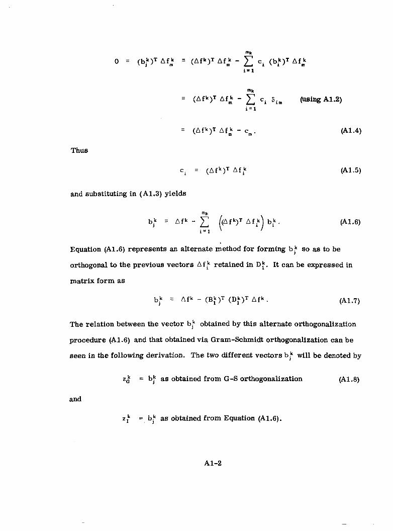
mk

= ( A f k ) T Af: - ci si, (using A-1.2) i = l

= ( A f k ) T A f t - cm. (Al.4)

Thus

'i = ( A f k ) T A f f (Al.5)

and substituting in (A1.3) yields

b; = A f k - 2 ((Afk)' Af:) bk (Al.6)

Equation (A1.6) represents an alternate method for forming b4 so as to be

orthogonal to the previous vectors A f k retained in D :. It can be expressed in

matrix form as

br = A f k - (B:)T (D:)T A f k . (Al.7)

The relation between the vector br obtained by this alternate orthogonalization

procedure (A1.6) and that obtained via Gram-Schmidt orthogonalization can be

seen in the following derivation. The two different vectors bf will be denoted by

z t = bf as obtained from G-S orthogonalization (Al.8)

and

2: = bf as obtained from Equation (A1.6).

A1-2

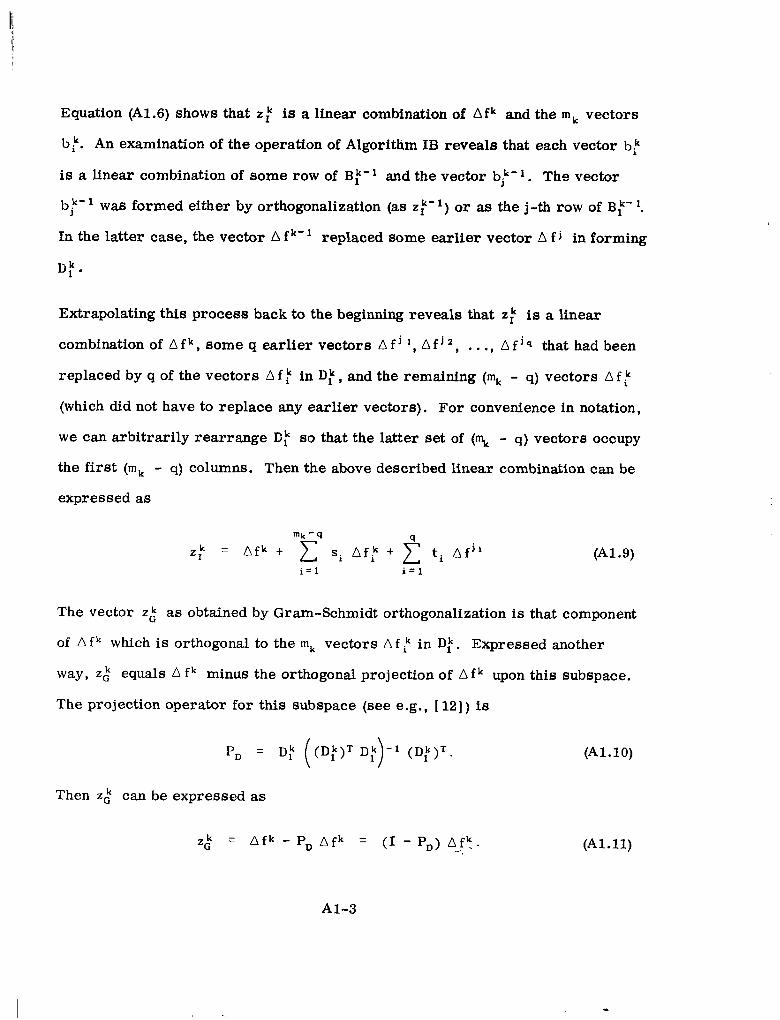
Equation (A1.6) shows that z: is a linear combination of A f k and the m k vectors

bk. An examination of the operation of Algorithm IB reveals that each vector bk

is a linear combination of some row of I3f-l and the vector bj"''. Ths vector

b;-' w a s formed either by orthogonalization (as z:") or as the j-th row of Bf'l.

In the latter case, the vector A f k- ' replaced some earlier vector A f j in forming

D f . Extrapolating this process back to the beginning reveals that z: is a linear

combination of A f k , some q earlier vectors A f j ',A f ' l , ..., A f j q that had been

replaced by q of the vectors A f in Df,and the remaining (mk - q) vectors A f k (which did not have to replace any earlier vectors). For convenience in notation,

w e can arbitrarily rearrange D: so that the latter set of (% - q) vectors occupy

the first (mk - q) columns. Then the above described linear combination can be

expressed as

(A1.9)

The vector z k as obtained by Gram-Schmidt orthogonalization is that component

of A f k which is orthogonal to the mk vectors A f k in D:. Expressed another

way, z k equals A f k minus the orthogonal projection of A f k upon this subspace.

The projection operator for this subspace (see e.g., [ 121) is

P, = D: ( (D,k)T D;)-l (D:)=. (A1.10)

Then z i can be expressed as

(A 1.11)

A1-3

-

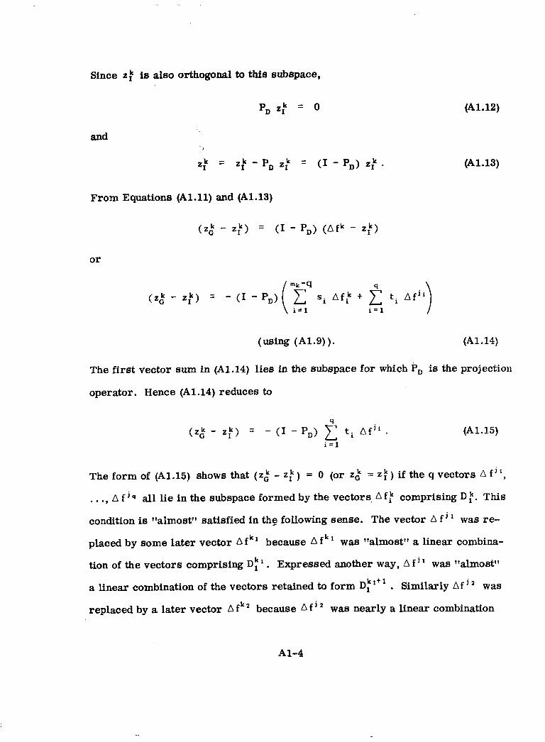
Since zf is also orthogonal to this subspace,

PD 2; = 0 (A1.12)

and

2; = 2: - P, 2: = (I - P,) 2:. (A1.13)

From Equations (Al . l l ) and (A1.13)

( 2 6 - 2:) = ( I - P,) ( A f k - 2:)

or

(using (Al.9)). (A1.14)

The first vector sum in (A1.14) lies in the subspace for which P, is the projection

operator. Hence (A1.14) reduces to

9

(2; - 2;) - - (I - PD) C t i A f J i . (A1.15) i = l

The form of (A1.15) shows that (2," - z:) = 0 (or z k J z:) if the q vectors A f ' * ,

...,A f J q all lie in the subspace formed by the vectors, A f comprising D t. This condition is llalmost'l satisfied in the following sense. The vector A f j w a s re­

placed by some later vector A f k l because A f k ' was llalmostlla linear combina­

tion of the vectors comprising D: . Expressed another way, A f 1 was "almost"

a linear combination of the vectors retained to form D,k i t 1 . Similarly A f j w a s

replaced by a later vector A f k 2 because A f J

w a s nearly a linear combination

A1-4

-

s

of the vectors retained to form Dlkz+l ,etc. Then the vectors A f j * , ...,A f j q

are t'almostttin the subspace of the vectors comprising D: so that (2," - 2:) 2 0.

The smaller p1 is in the criterion of (2.5), the closer is this approximation.

At k = p when n - 1independent vectors A fp have been retained in D p, zf' (if

it is non-zero) wil l be the same as z&' (to within a scalar multiple which is

irrelevant) , regardless of whether o r not the replaced vectors A f j' are in the

subspace spanned by the columns of D 1". This subspace would be of dimension

n - 1,and since both z p and zGp are orthogonal to this subspace, they both must

lie along the same line in n space. More formally, referring to (A1.15), 1 t i A f "

lies in n space and can be expresaed as a linear combination of A f P and the n - 1

vectors comprising Df'. But (I-P,,) operating on this linear combination yields

zero everywhere except for the component along A f P ,or

- - ,u (using (Al.11))

or

z p = (1 + p ) z& (A 1.16)

If no earlier vectors A f " have been replaced up to the k-th instant, then (A1.15)

implies that z$ = z f . This is always the case in (Secant) Algorithm IB-S. Hence

the use of the alternate orthogonalization procedure of (A1.6) in Algorithm IB-S

yields identical resultP tr, those obtained by Gram-Schmidt orthogonalization.

The same orthogonalization procedure just described can also be used in Algo­

rithm IIB to form the trial vector a! satisfying

A1-5

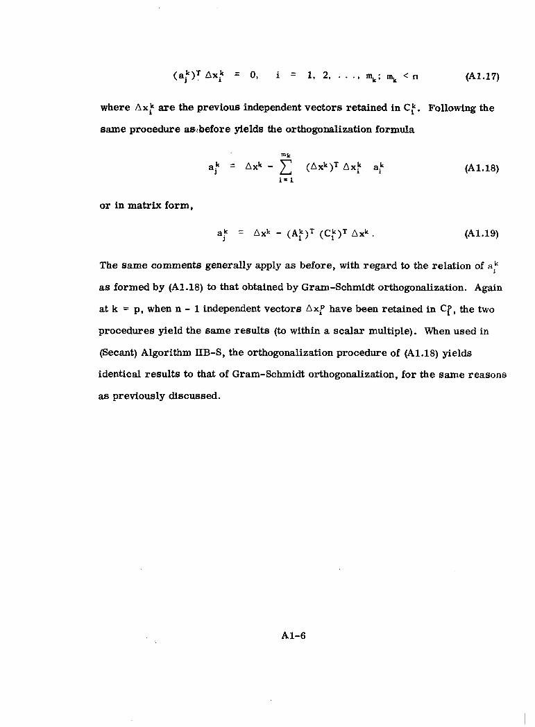
(a:)= Ax: = 0, i = 1, 2, . . . , 2;mk < n (A1.17)

where Ax: are the previous independent vectors retained in Cf. Following the

same procedure a&before yields the orthogonalization formula

(A 1.18)

o r in matrix form,

1ak = A x k - (A:)= (C:)T Axk. (A1.19)

The same comments generally apply as before, with regard to the relation of a:

as formed by (Al.18) to that obtained by Gram-Schmidt orthogonalization. Again

at k = p, when n - 1independent vectors Ax: have been retained in Cf,the two

procedures yield the same results (to within a scalar multiple). When used in

(Secant) Algorithm IIB-S, the orthogonalization procedure of (A1.18) yields

identical results to that of Gram-Schmidt orthogonalization, for the same reasons

as previously discussed.

A1-6

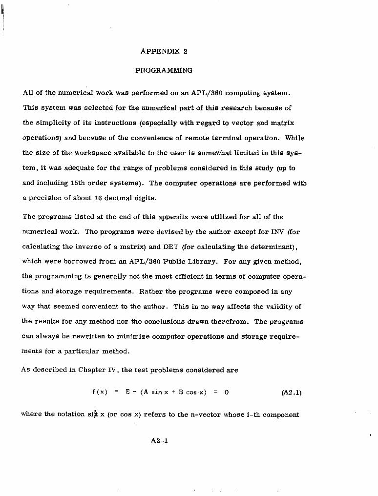
APPENDIX 2

PROGRAMMING

All of the numerical work w a s performed on an APL/360 computing system.

This system w a s selected for the numerical part of this research because of

the simplicity of its instructions (especially with regard to vector and matrix

operations) and because of the convenience of remote terminal operation. While

the size of the workspace available to the user is somewhat limited in this sys­

tem, it w a s adequate for the range of problems considered in this study (up to

and including 15th order systems). The computer operations are performed with

a precision of about 16 decimal digits.

The programs listed at the end of this appendix were utilized for all of the

numerical work. The programs were devised by the author except for INV (for

calculating the inverse of a matrix) and DET (for calculating the determinant),

which were borrowed from an APL/360 Public Library. For any given method,

the programming is generally not the most efficient in terms of computer opera­

tions and storage requirements. Rather the programs were composed in any

way that seemed convenient to the author. This in no way affects the validity of

the results for any method nor the conclusions drawn therefrom. The programs

can always be rewritten to minimize computer operations and storage require­

ments for a particular method.

As described in Chapter IV , t he test problems considered are

f(x) = E - (A s i n x + B c0s.x) = 0 (A2.1)

where the notation si%x (or cos x) refers to the n-vector whose i-th component

A2-1

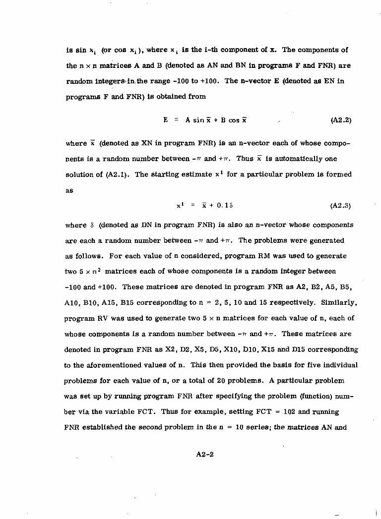
is sin xi (or cos xi),where x i is the i-th component of x. The components of

the n x n matrices A and B (denoted as AN and BN in programs F and FNR)are

random integers+@therange -100 to +loo. The n-vector E (denoted as E N in

programs F and FNR)is obtained from

E = A s i n E t B c o s Z (A2.2)

where x (denoted as XN in program FNR) is an n-vector each of whose compo­

nents is a random number between - - 7 ~ and +n. Thus x is automatically one

solution of (A2.1). The starting estimate x for a particular problem is formed

as

x1 = x t 0.18 (A2.3)

where 6 (denoted as DN in program FNR) is also an n-vector whose components

are each a random number between -n and +n. The problems were generated

as follows. For each value of n considered, program R M w a s used to generate

two 5 x n2 matrices each of whose components is a random integer between

-100 and +loo. These matrices are denoted in program FNR as A2,B2,A5,B5,

A10,B10,A15,B15 corresponding to n = 2, 5, 10 and 15 respectively. Similarly,

program RV w a s used to generate two 5 x n matrices for each value of n, each of

whose components is a random number between -n and +T. These matrices are

denoted in program FNR as X2,D2,X5,D5,X10,D10,X15 and D15 corresponding

to the aforementioned values of n. This then provided the basis for five individual

problems for each value of n, or a total of 20 problems. A particular problem

was set up by running program FNR after specifying the problem (function) num­

ber via the variable FCT. Thus for example, setting FCT = 102 and running

FNR established the second problem in the n = 10 series; the matrices AN and

A2-2

BN would be formed from the second rows of A10 and B10 respectively while

the vectors XN and DN would be formed from the second rows of X10 and D10

respectively. The initial value x1 (denoted as X1 in FNR)would also be estab­

lished as per (A2.3).

Once a problem w a s set up, an approximation H' to the inverse Jacobian at x1

(denoted as JX1) w a s formed via program JINV, which formed a discrete approxi­

mation to the Jacobian via program F and calculated the inverse via IM. The

discretization parameter h w a s specified as lom4 (via DEL). The matrix denoted

as E in JINV is the identity matrix of order n. Then a particular run was speci­

. fied by assigning component values to the vector variable SEL, which selected

among other things the particular algorithm to be used, the quasi-Newton step

(full step w a s used throughout, i.e., ak = l), the maximum number of iterations

permitted, the convergence criterion for (1 fk \ I 2 (set at lom6throughout), and the

value of p1 for use in Algorithm I o r Algorithm II. The parameter p 2 in Algo­

rithm I1 w a s arbitrarily fixed at 0.1 pl .

The program BEGIN started a particular run. This program printed out several

items for run identification purposes including the algorithm used, the function

(problem) number, and the selected value of p1 (when Algorithm I or Algorithm II

w a s utilized). This program also incorporated the programs INITIAL and

ITERATE. The program INITIAL established initial values for several variables

and ITERATE performed the actual iterations. Included in ITERATE are pro­

grams AMEND and HNEW. The program AMEND formed Axk, x k + l, f k + l ,and

A f k in the usual way, for subsequent use. The program HNEW then formed Hk+

according to the particular algorithm that had been selected. For example in the

discrete Newton's Method (ALG = 9), I l k + ' w a s formed as an approximation to

A2-3

I

J' (xktl ) using the program JRW . For the other methods, HNEW selected the

appropriate program for calculating Hk + . After calculation of Hk l , the execu­

tion returned to ITERATE where the iterate index k was incremented by one.

After a check for convergence of 11 f k 11, and for determination of whether k ex­

ceeded the allowable limit, the process was repeated.

Besides a discrete Newton's Method, the other methods used on each problem

were Broyden's Methods 1and 2 (ALG = 7 and ALG = 8 respectively), Secant

algorithms I-S and 11-S (ALG = 5 and 6 respectively), a combination of Broyden's

Method 1and Algorithm 11-S (ALG = lo), Algorithm I (ALG = l), and Algorithm 11

(ALG = 2). There was also provision for using Algorithms I and I1 with Gram-

Schmidt orthogonalization (ALG = 3 and 4 respectively) but this was only used

on a few problems since the computations were more extensive and there was

generally little if any improvement over the simpler alternate orthogonalization

scheme. The program names for forming Hk+lin accordance with the afore­

mentioned methods are BROYDEN, SECANT, BRlALGIIS, ALGI, and ALGII.

program SECANT includes Algorithms I-S and 11-S. When Algorithm I-S (II-S)

is used, Algorithm IB-S (IIB-S) is in effect until k = n + 1at which time a switch

is made to Algorithm IA-S (IIA-S). Similarly, in program ALGI (or ALGII), Algo­

rithm IB (IIB) is in effect until mk = n at which time a switch is made to Algo­

rithm IA (IIA). The operation of programs ALGI and ALGII wil l be described in

the following paragraphs, with the program variables identified in terms of the

nomenclature used elsewhere in this report. The description should also suffice

to clarify the operation of the similar but simpler program SECANT.

When Algorithm IB (IIB)is in effect, the vector 2,representing b: (a;), ie

formed first via an orthogonalization procedure. If the appropriate criteria are

A2-4

I

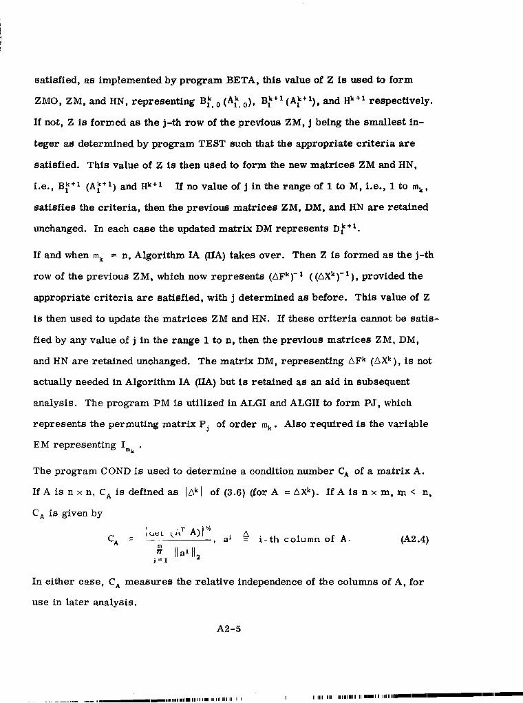
satisfied, as implemented by program BETA, this value of Z is used to form

ZMO, ZM, and HN, representing Bt, (A:, o ) , B:+I (A,k+l) , and Hk+lrespectively.

If not, Z is formed as the j-th row of the previous ZM, j being the smallest in­

teger as determined by program TEST such that the appropriate criteria are

satisfied. This value of Z is then used to form the new matrices ZM and HN,

i.e., B;+I (Alk'l) and Hktl If no value of j in the range of 1 to M, Le., 1to mk,

satisfies the criteria, then the previous matrices ZM, DM, and HN are retained

unchanged. In each case the updated matrix DM represents D: 'l .

If and when mk = n, Algorithm IA (IJA) takes over. Then Z is formed as the j-th

row of the previous ZM, which now represents (AFk) - l ( (AXk)-') , provided the

appropriate cri teria are satisfied, with j determined as before. This value of Z

is then used to update the matrices ZM and HN. If these criteria cannot be satis­

fied by any value of j in the range 1to n, then the previous matrices ZM, DM,

and HN are retained unchanged. The matrix DM, representing A F k ( A X k ) , is not

actually needed in Algorithm IA (IIA)but is retained as an aid in subsequent

analysis. The program P M is utilized in ALGI and ALGII to form PJ, which

represents the permuting matrix Pj of order mk . Also required is the variable

E M representing Imk. The program COND is used to determine a condition number C, of a matrix A.

If A is n x n, C, is defined as ( A k [ of (3.6) (for A = AXk). If A is n x m, m < n,

C, is given by

c, = ; ~ C L(AT A ) ] ' , ai 4 i - t h column of A . (A2.4)

m Ilai112

i = 1

In either case, C, measures the relative independence of the columns of A, for

use in later analysis.

A2-5

~ ~ -.. ....___.--.-- 11.1 -11.1111111.111.1111111 1111 11111 I I

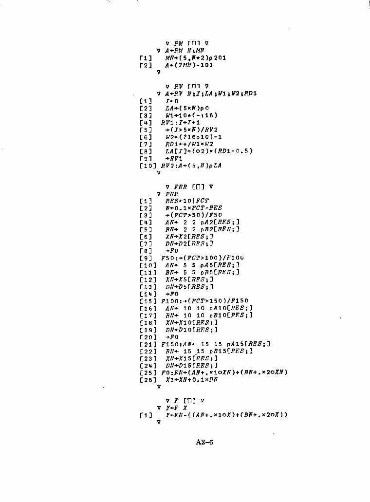
0 RV fn1 V V A+RV N;I;LA;Wl;WP;RDl

c11 140 [2] LA+(SxN)pOC3] W1+10*(-\16)C41 RV1:I+I+l f 5 3 +(1>5xN)/RV2 C61 W2+(?16p10)-1C 73 RDl++/ h?lx 112 C 81 LA[l]+(o2)x(RDl- 0 . 5 ) r91 + m i [lo] RV2:A+( 5 ,N)pLA

V

v FNR cni v V FNR

Cl I RES+lOIFCT c 2 1 N+O.lxFCT-RES C 3 1 +(FCT>50)/F50 C41 A N 4 2 2 pA2CRES;I C 5 1 RN+ 2 2 pB2CRPS;l C61 XN+X2CRBS;l C71 DN+D2CRES;l 1-83 +FO C91 F50:+(FCT>100)/FlO~C101 A N 4 5 5 pA5CRES;IC111 BN+ 5 5 pB5CRBS;l c 12 3 XN+XS c RES;3 Ti31 DN+D5[RES;]C141 +FO C l S I F100:+(FCT~lSO)/FlSOC161 AN+ 10 10 pA1OCRES;IC17'1 RN+ 10 10 pBlOCRRS;] C18l XN+XlOCRRS;]Cis1 DN+DlOCRES;l f201 +FO C213 FlSO:AN+ 15 15 pAl5CRES;lC221 RN+ 15 15 pB15CRES;JC 23 1 XN+Xl5 (RES;1 C241 DN+DlSCRES;I C 2 5 1 FO:BN+(AN+.xlOXN)+(RN+.x2oXN) C261 Xl+XN+O.lxDN

V

V F COI V v Y4F X

I-11 Y+BlV-((AN+.xloX)+(BN+.x2oX))V

A2-6

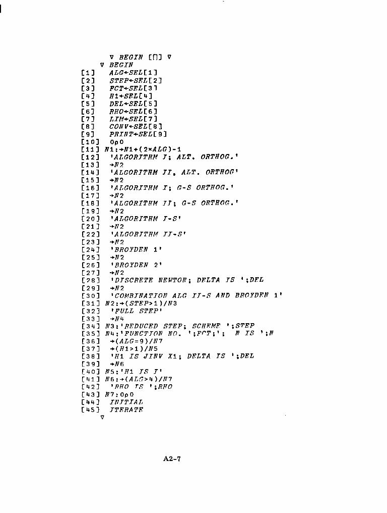
V BEGIN Cnl V V BEGIN

I:1 I ALG+SBL C 1I C 2 3 STRP+SEL I:2 1 C 3 3 FCT+SBLC 3 7 C41 Hl+SELC 43 I:5 1 BEL+SELC 5 1C 6 3 RHOtSELC 6 I C 7 3 LIW-SELC7 3 CSl CONV+SELCBI C93 PRINT+SELCSI El01 o p o [ill Nl t+Nl+( 2xALG)-l C 1 2 1 ‘ALGORITHM 7;ALT. ORTROG,‘ E 1 3 1 + N 2 C141 ‘ALGORJTRM JI, ALT. ORTROC‘ C151 + N 2 [I61 ’ALGORITHM I ; C - S OPTHOG.‘ C171 +N2 C I S 1 ‘ALGORITHM IT; C - S ORTHOC.‘ [I91 + N 2 C201 ‘ALGORZTHM J - S ‘ E 2 1 1 4 7 2 [2 2 1 ‘ALGORTTHP! T T - S ‘ C 2 3 1 -072 C241 ‘BROYDEN 1’ [251 +N 2 E 2 6 1 ‘BROYDEN 2’ C271 + N 2 C701 ‘DTSCRKTE NEWTON; DELTA T S ‘;DFL C 2 9 1 4 N 2 C301 ‘COMRTNATTON ALG T J - S AND BROYDFN 1 ’ C 3 1 l N2:+(STEP>l )/N3 E 3 2 1 ‘ F U L L STEP‘ C 3 3 1 4 N 4 c341 N3:’REDUCED S T E P ; SCHEME ’ ; S T E P [3S] N4:’FUNCTJON NO. ‘;FPT;’; N TS ’;I? C 3 6 1 +(ALG=9)/N7 C 3 7 1 + ( H I > l ) / N S c 3 0 1 ’ H I IS JTNV XI; DELTA TS ‘;DEL C 3 9 1 +N6 C401 N5:‘HI TS J ’ C 4 l l N6:+(ALC>4)/N7 C 4 2 1 ’RHO T S ‘;RPO C431 N 7 : O p O C441 ZNJTTAC C451 JTERATE

V

A2-7

V I N I T I A L [n] V V I N I T I A L

Cll NX+XI C23 FNX+F RX C31 MFNX++/FNXxFNXC 41 K+M+Q+L+OC 5 1 DM+Np 0 [SI ZM+BDM C71 +(Hl=l ) / I N C 81 HN+E c91 +o C 101 I N :HN+JXl

V

V I T E R A T E [ P I V V I T E R A T E

[ll TTER:X+NX [23 FX+FNX C31 H+HN C 4 1 MAGF+MFNX C 5 1 K+K+I [6] 'K! ';K;'* NORM OF F X : ' ; M A C F * 0 . 5 C71 + ( P R I N T < B i / L T C81 + ( ( 5 1 K ) * O ) / L T C9l 'COND. N O . OF H : ' ; C O N D H C101 ' D E T OF H: ' ; D T C113 + ( A L C > f i ) / L T C 1 2 1 'COND. N O . OF RM: ' ; C O N R DM C131 ' D E T OF D M : ' ; D T E 1 4 1 L T : + ( (MACF*O. 5 ) < C O N V ) / S O L C i s 1 + ( P R I N T < l ) / L T l cis1 ' M A X DIFF FROM EXPFCTED S O L : ' ; r / I x - x u C171 + ( P R I N T < 2 ) / L T I [ l a ] 'MAX D I F F BETWE'RN H APD JXNV A T S O L I ' ; r / l ( A x A ) o ( H - J X F ) [ i s ] L T l : + ( K > L I M ) / T E R M [ 2 0 ] P+-H+.xFX C211 AMEND C221 HNEW C231 + I T E R c 24i TERM:'TERMINATED ; N O . OF TTERATIONS E X C F E D S L r ! m * C 2 5 1 +END C76l S0L:QpO E271 + ( N > S ) / L T 5 1281 ' SOLUTION I S : ' C291 X E301 L T 5 : ' M A X D I F F FROM EXPECTED S O L : ' ; r / l X - X N [31] 'MAX A B S ERROR I N APPR J.TNV A T S O L : ' ; T / l ( f l * W ) p ( R - J X F ) C321 + ( P R I N T < 4 ) / E N D C331 'APPROX JXNV AT SOLUTION: ' C341 H C351 END; 3 0 P O

V

A2-8

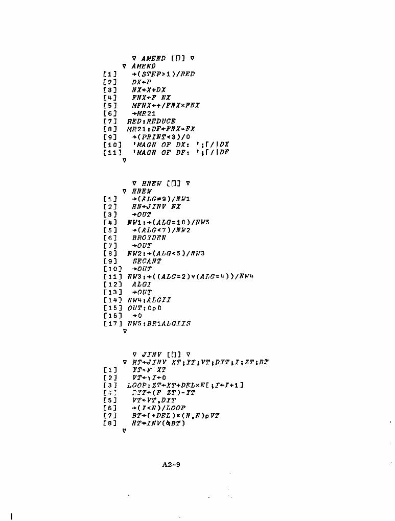
0 AMEND CUI Q 0 AMEND

C l J +(STBP>I )/REDC 2 3 DX+P C3 3 NX+X+DX C Q 3 FNX+F NX [5 3 MFNX++/FNXxFNX C63 +MR21 C 7 3 RED t REDUCE CSl MR21:DF+FNX-FX C93 +(PRINT<3)/0 C l 0 3 'MACN OF DX: ,;T/(DX C111 'MACN OF DF: * ; r / ( D F

Q

0 HNEW Cnl V 0 HNEW

C11 +(ALG*9)/NW1C 2 3 RN+JINV NX C33 +OUT C43 NWlr+(ALG=IO)/NWS[SI +(ALG<7)/NW2 [61 BROYDEN C71 +OUT E 0 1 NW2:+(ALG<5)/lQW3 L93 SECANT E l 0 3 +OUT c 11 3 NW3 t + ( (ALC=2) v ( A L C = Q ) )/NY4E123 ALGI C I S 3 +OUT C 141 N W 4 :ALG.TI C153 0UT:OpO C161 + O C171 NW5:BRIALGIIS

V

0 JINV C f l l V V HT+JINV XT;YT VT;DYT;I;2T;BT

E 1 3 YT+F XT C 2 1 VT+iI+O [3 1 LOOP: ZT+XT+DELxEC ;I+I+i3 [:;I ?YT+( F ZT)-YT C 5 3 VT+VT,DYT [SI +(I<N)/LOOPC 7 3 BT+( +DRL)x (N,N )p VT E 8 3 RT+INV(4BT)

0

A2-9

0 S E C A N T CUI V 0 SECANT ;(I; V;2 ;ZDV;ZMO ;PJ ;DMO

C l I V+DX-R+.xDP C 2 1 +(ALG=6)/S2 C 3 1 Sl:DV+DF c43 +s3 CS3 S2rDV+DX C6 1 S3 :+( K>N )/S4 c 7 3 Z+DV- (4 ZM )+ .x (@DM)+ xDV C B J ZDV++/ZxDV c 9 3 ZMO+ZM- ( iZDV)x ( ZM+ .xDV)e . x Z C 10 I ZM+( K,IV )P ( (NxK- I )p ZEiO ) Z + ZDV r 11 I DM+it+( K , A )p ( ( NxK-1 InqDM),DVc 1 2 1 +s5 C13 I S4 :Z+ZMCl; 1 E141 BM+(N,R)pi,NpO C l S 1 ZMO+ZM+(~+/ZxDV)x(EMCl;J-ZM+.xDVI. .xz C161 M+N C17 3 PJ+PM 1 C l B J ZM+PJ+.xZMO C191 D M O + ~ M + ( D V - D M [ ; ~ I ) O . X E M ~ ; ~ ] C 2 0 1 DM+DEfO+. x (QPJ) C 2 1 1 SS:+(ALG=6)/S6 [ 2 2 ] v+Z E 2 3 1 +'S7 E241 S6rV+(@H)t.xZ C 2 5 1 S7:HN+Ht(i+/VxDF)xUo.xV

V

V B R l A L G I I S [n] V V BR1ALGIIS;U;V;Z;ZDV:ZMQ;PJ;nMO

C l I U+DX-H+. xDF C 2 1 DV+DX C31 +(K*N)/SR4 C41 Z+DV-(BZM)+. x (4DM)+. xDV E 5 1 ZDV++/ZxDVC 6 I ZMO+ZM- ( + ZDV)x ( ZM+. xDV)0 . X Z C 7I ZM+( K ,N )p ( ( N x K -1)p ZMQ ) ,Z i ZDV C 8 1 L'M+Q( K,N )p ( ( NxK-1 ) o Q n M ) ,Dt c 9 1 +SR5 c 1 0 1 SR4:Z+ZMCl;l t 11 I E)?+( A ,ir )p i , ~ po C 1 2 1 ZMO+ZM+( + t/i>DV)x (EMT1;I-ZM+. xDV 10 . X Z C 1 3 1 M+N C l 4 1 PJ+PM 1 C 15 1 ZM+PJ+ .x ZE?O [161 DMO+DM+( DV-DMC ;1 7 ) e . xEMr ;1 3 C171 DM+DMO+. x ((PPJ) C l S I SRS:ZC+0.5x(ZtDV) ti91 V+fQH)t.xZC [ 2 0 ] HN+H+(+t/VxDF)xNo. XV

V

A2-10

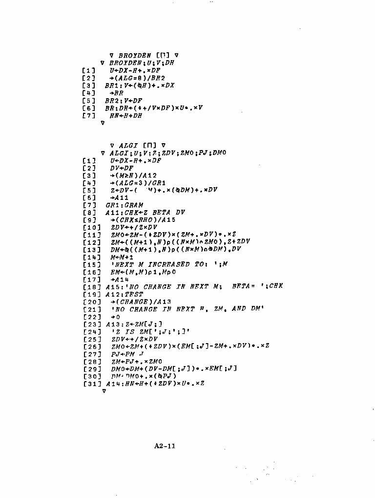
V BROYDEN [[?I V V BR0YDEA;U;V;DH

[13 U+DX-R+.xDF C23 +(ALG=8)/BR2 t 3 1 BRI t V+( (PH)+ .xDX C43 +BR C 5 3 BR2:V+DF [SI BR:DH4(++/VxDF)x~ooXV [7] RN+H+DH

V

V ALGI En] V V ALGI ;U ;V ;7: ;ZDV ;ZMO ;PJ ;DMO

C l I U+DX-R+.xDF E21 DV+DF C3l +(MZN)/A12C41 +(ALC=B)/GRlC 5 3 Z + D V - ( ' Y ) + . x (QDM)+.xDV C63 +All C73 GR1:CRAM CSl AlltCBK+Z BETA DV C 93 + ( C R K s R H O )/A15 C103 ZDV++/ZxDV CY.1 ] ZMO+ZM-( + ZDV)x ( ZM+ .xDV)0 . X Z C f 21 ZM+( ( M i l 1, N ) p ( ( N x M 1n ZMO ) ,2t ZDV C13 3 DM+.4( (M+l),N ) p ( (NxM) n ( P D M ) ,DV [ I 4 3 M+M+l C153 'NEXT M INCREASED TO: ';M [:163 EM+(M,M)p 1 , M p 0 C171 +A14 C.181 A15:'NO CHANCE IN NEXT M ; BETA= ' ; C H K C191 A12 ;TEST C 201 +(CHANGE)/Ai3 C211 'PJO CHANGE Tlll NEXT R, ZM, A R D D#' C 2 2 1 +o C233 A13: Z+ZMCJ;I C241 '2 IS ZMC';J;'*9 3 ' C 2 5 3 ZDV++ / Z x D V I:26 J Z M O + Z M + ( .IZ D V ) x (EM[ J J I -ZM+. xDV 1 0 . x 2 E271 PJ+PM -7 C281 ZM+PJ+.xZMO [:293 DMO+DM+ (DV-DMC;J ]10. xEMC ;J ] [3 0) PPI. ?MO+. x ((PPJ) C3 11 A14 :HN+H+ ( + ZDV ) x U o . x Z

V

A2-11

V A L C I I [ I l l V V A L C I I iU iV ; Z ; Z O V ; ZMO :PJ;DMO

E l ] U+DX-H+.xDF C 2 I DV+DX c 3 +(MLN / A 2 2 r 4 1 + ( A L G = 4 ) / C R 2C 5 1 Z+DV- ( Q Z M ) + . x ( (PDM)+. XVV C 6 l + A 2 1 1 7 1 CR2:CRAM C 8 1 A 2 1 : C H K l + Z B E T A DV C93 C H K 2 + ( ( Q H ) + . x Z ) BETA DF [1 0 1 +( CHKlsRRO ) / A 2 5 C111 + ( C H K 2 S O . l x R H O ) / A 2 5 r i 2 1 Z ~ V + + / Z X D V r 1 3 1 ZMO+-ZM-(+ZDV)x(ZM+.xDV)o.xZ r 1 4 1 ZPf+((M+i),N)p( ( N x M ) n Z M O ) , Z + Z D V r l 5 l DM+Q( ( M + l ) , N I P ( (NxM)nQDEA) ,DVC 16 1 M+M+l C171 ' N E X T M TNCRFASED T O ; ' ;M r 1 8 1 EM+( M , M ) p l , M p 0 r i g 1 + A 2 4 r 2 O I A 2 5 : ' N O CHANCE J N NRXT M ; CAMiVA= ' ; C B K I ; ' , B E T A = ' : C H K 7 C21 I A 2 2 : T E S T r 2 2 1 +( CRANCE: ) / A 2 3 f 2 3 1 ' N O CHANCE: TN NEXT H , ZM, AND DM' r 2 4 1 +O -. f 2 5 1 A 2 3 :Z+ZMC J ;3 r 2 6 1 'Z I S ZMC';J;';I' f 2 7 I Z D V++ / Zx D V r 2 8 I ZMO*-ZM+( + Z D V ) x (EM[:J J - Z M + .X D V ) o X Z C291 PJ+PM J r 3 0I ZM+PJ+. x Z M O C 3 1 3 D M O ~ D M + ( D ~ - D M C ; J ] ) O . X ~ ~ ~ ~ ; J ~ C3 2 1 DM+DMO+. x ( (PPJ 1 f 3 3 1 A 2 4 : V + ( 4 H ) + . x Z r 3 4 l + ( P R I N T < 7 ) / A 3 3 C 3 5 1 '1-ZMxDM: ' ;r / I(M x M )p (EM- ZM+ .xDM ) r 3 6 3 A 3 3 :HN+H+ ( + + / V x D F )x N o . x V

V

A2-12

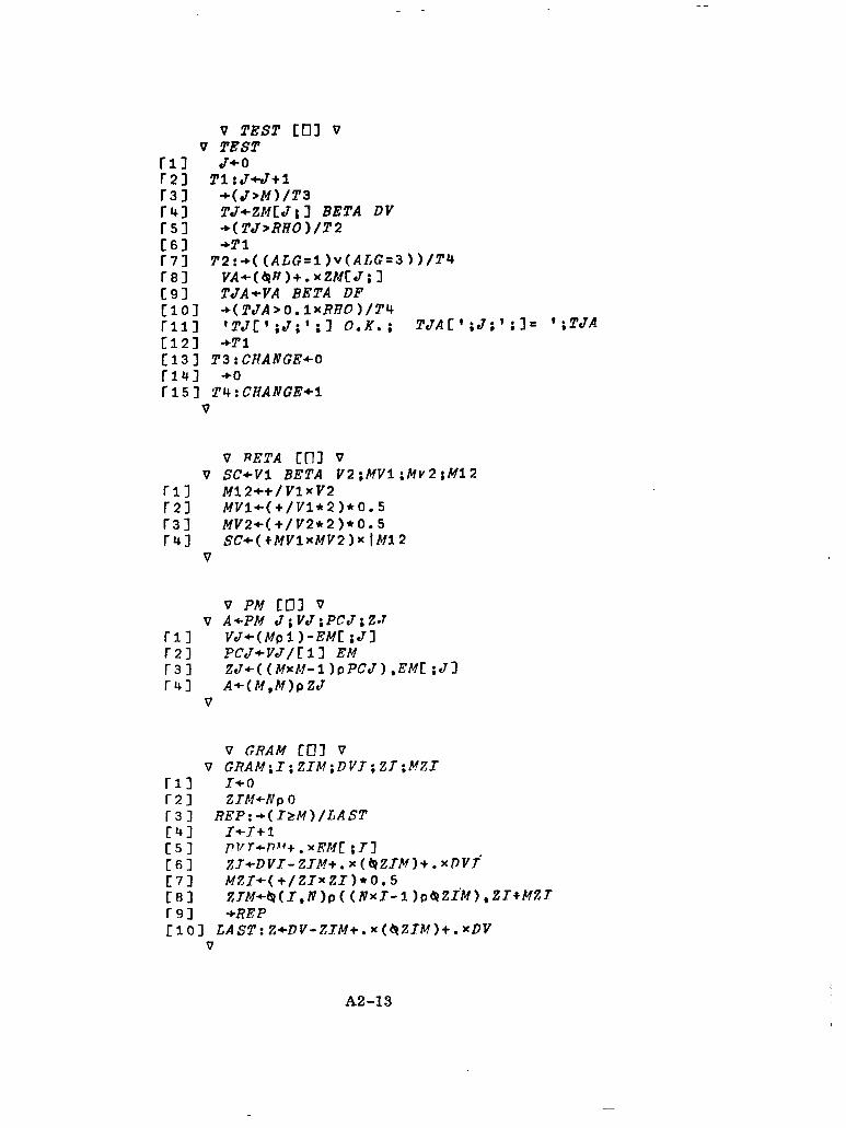
0 TEST CUI 0 0 TEST

r i i J+O r21 Tl:J+J+l r 3 3 +(J>M)/T3r41 TJ+ZMCJ;l BETA DV T5 3 +(TJ>RHO)/T2 E63 +Ti r 7 1 T2:+( (ALG=l)v(ALG=B))/T4r 83 VA+( 4 H )+. x ZMCJ ;I C93 TJA+VA BETA DF C103 +(TJA>O.lxRRO)/T4f l l l 'TJ[';J;';I O . K . ; TJAC';J;';l= ';TJA C121 +T1 C131 TB:CHANCE+O ri41 +O r 15 3 Tls :CHANCE4

0

v RETA COI v 0 SC+Vl BETA V2;MVl;kv2;Ml2

r i l M ~ ~ + + / v I x v ~r21 M V I + ( + / V ~ * ~ ) * O . ~r 3 3 ~ V 2 4+/V2*2 ) *0.5 r41 SC+(+MVlxMV2)xlM12

V

PM CUI V V A+PM J;VJ;PCJ;ZJ

r 1 3 VJ+(Mpl)-EMC;Jl r21 PCJ+VJ/CIl EM r 3 1 ZJ+((MxM-l)pPCJ),EMC;Jl r 43 A+(M,M )p ZJ

V

0 CRAM CUI V V CRAM;Z;Z1M;DVJ;Z ; T ; E A Z I

r i i 11-0 r 21 ZZM+Np 0 r31 REP:+(IzM)/LASTC41 I+J+1 [ 5 3 PT'T+nn'+. xFM[ ;TJ C 61 ZI+DVZ- ZJM+ .x ( 4 Z m )+ .xOVf C 7 3 Mer+( +/ZIxZI)*0 . 5 C 8 I ZJM+4 ( I,R )p ( ( NxI-1 )p 4 ZIM ) ,ZI.)MZT r91 +REP ClOI LAST:Z+DV-ZIM+.x(@ZIM)+.xDV

V

A2-13

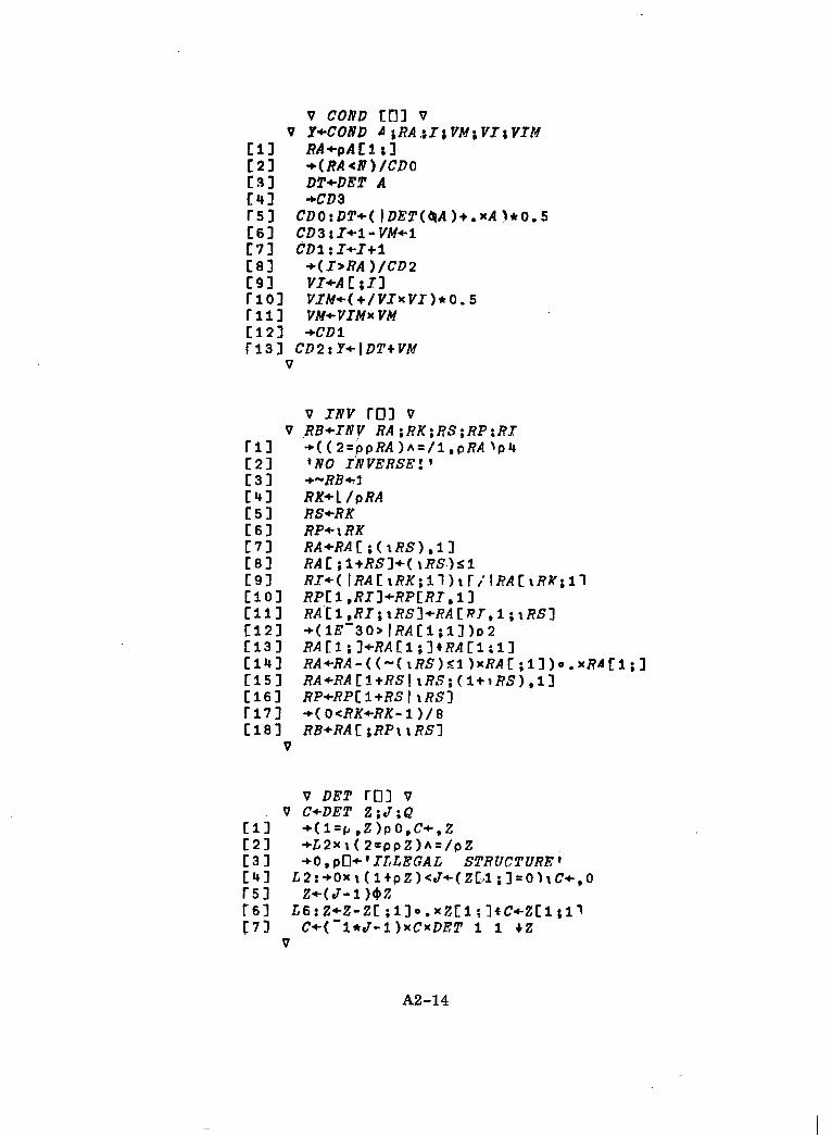
V COND 6131 V V Y+COND A ;RA;I;VM;VI;VIM

C 11 RA+pA C 1;1 C21 +(RA4V)/CDO C33 DT+DET A C43 +CD3 r 5 3 CDO t DT+( IDET(&A )+. xA !*O. 5 C S ] CD3:I+l-VM+l C71 CDl:I+I+i CS3 +(I>RA)/CD2 C91 VI+AC;Ilr 1o I VXM+( +/ V I x VI)* 0 . 5 f 11I VM+VIMx VM C121 +CD1 Ti33 CD2rY+JDTtVM

V

v INV roi v 0 RB+INV RA;RX;RS;RP:RI

r11 +( (2=ppRA)A=/l,pRA104 C21 @NO INVERSE!‘ C3 l +NRB+3 C41 RK+I /ORAC 5 1 RS+RK C 61 RP+ i RK C71 RA+RAC ;( I RS),11 CSl RAC;l+RSI+(rRS.)slC 9 1 RI+( IRA C 1RK;11) I r ;1 RA C IRK;11 C l O l RPCl,RII+RPCRI,ll c 111 RA [:1,RI;i RSI+RA C R J , 1 ;I RSI Cl23 +( 1E-30> IRAC 1 ;1110 2 C13 1 RAC1;I+RAC 1;1tRAC1:11 Cis1 RA+RA- ( ( - ( 1RS)ll )xRA[ ;13 ) e . x R ~[l;3 C15 1 RA+RA Cl+RS 1 i RS;( l+r R S ) ,lI C161 RP+RPCl+RS(iRSIr671 +(O<RK+RK-1)/8 L l S l RB+RAC;RPIIRSI

V

A2-14