Embed Size (px)
Citation preview
REVIEW ARTICLE
Nonlinear physics of electrical wave propagation in
the heart: a review
Sergio Alonso1,2, Markus Bar1, and Blas Echebarria2
1 Physikalisch-Technische Bundesanstalt, Abbestr. 2-12 10587, Berlin, Germany2 Department of Physics, Universitat Politecnica de Catalunya, Av. Dr. Maranon 44,
E-08028 Barcelona, Spain
E-mail: [email protected], [email protected], [email protected]
Abstract. The beating of the heart is a synchronized contraction of muscle cells
(myocytes) that are triggered by a periodic sequence of electrical waves (action
potentials) originating in the sino-atrial node and propagating over the atria and
the ventricles. Cardiac arrhythmias like atrial and ventricular fibrillation (AF,VF)
or ventricular tachycardia (VT) are caused by disruptions and instabilities of these
electrical excitations, that lead to the emergence of rotating waves (VT) and turbulent
wave patterns (AF,VF). Numerous simulation and experimental studies during the
last 20 years have addressed these topics. In this review we focus on the nonlinear
dynamics of wave propagation in the heart with an emphasis on the theory of pulses,
spirals and scroll waves and their instabilities in excitable media and their application
to cardiac modeling. After an introduction into electrophysiological models for action
potential propagation, the modeling and analysis of spatiotemporal alternans, spiral
and scroll meandering, spiral breakup and scroll wave instabilities like negative line
tension and sproing are reviewed in depth and discussed with emphasis on their impact
in cardiac arrhythmias.
CONTENTS 2
Contents
1 Introduction 4
2 Electrophysiology of the cardiac electrical activation 8
2.1 The heart . . . . . . . . . . . . . . . . . . . . . . . . . . . . . . . . . . . 8
2.2 The cardiac myocytes . . . . . . . . . . . . . . . . . . . . . . . . . . . . . 8
2.3 Electrical activity propagation . . . . . . . . . . . . . . . . . . . . . . . . 10
2.4 Cardiac arrhytmias . . . . . . . . . . . . . . . . . . . . . . . . . . . . . . 11
3 Mathematical description of the action potential propagation 13
3.1 Action potential . . . . . . . . . . . . . . . . . . . . . . . . . . . . . . . . 13
3.1.1 Nernst potential. . . . . . . . . . . . . . . . . . . . . . . . . . . . 13
3.1.2 Ion currents. . . . . . . . . . . . . . . . . . . . . . . . . . . . . . . 13
3.2 Connection among cells . . . . . . . . . . . . . . . . . . . . . . . . . . . 15
3.2.1 Intracellular action potential propagation. . . . . . . . . . . . . . 15
3.2.2 Intercellular action potential propagation. . . . . . . . . . . . . . 17
3.2.3 3D formulation. . . . . . . . . . . . . . . . . . . . . . . . . . . . . 18
3.3 Ionic models . . . . . . . . . . . . . . . . . . . . . . . . . . . . . . . . . . 19
3.3.1 Detailed electrophysiological models. . . . . . . . . . . . . . . . . 20
3.3.2 Cardiac models with simplified ion currents. . . . . . . . . . . . . 22
3.3.3 Generic reaction-diffusion models. . . . . . . . . . . . . . . . . . . 24
3.4 Excitation-contraction coupling . . . . . . . . . . . . . . . . . . . . . . . 25
3.4.1 Excitation-induced contraction . . . . . . . . . . . . . . . . . . . 26
3.4.2 Stretch activated channels. . . . . . . . . . . . . . . . . . . . . . . 26
3.5 Anisotropy. . . . . . . . . . . . . . . . . . . . . . . . . . . . . . . . . . . 27
3.5.1 Modeling three-dimensional anisotropy. . . . . . . . . . . . . . . . 27
4 Wave propagation in models of cardiac tissue 29
4.1 Homogeneous isotropic tissue . . . . . . . . . . . . . . . . . . . . . . . . 29
4.1.1 Traveling waves. . . . . . . . . . . . . . . . . . . . . . . . . . . . . 30
4.1.2 Spiral waves. . . . . . . . . . . . . . . . . . . . . . . . . . . . . . 33
4.1.3 Scroll waves. . . . . . . . . . . . . . . . . . . . . . . . . . . . . . . 35
4.2 Heterogeneous tissue . . . . . . . . . . . . . . . . . . . . . . . . . . . . . 36
4.2.1 Large non-excitable local heterogeneities. . . . . . . . . . . . . . . 36
4.2.2 Gradients of electrophysiological properties. . . . . . . . . . . . . 37
4.2.3 Localized heterogeneity. . . . . . . . . . . . . . . . . . . . . . . . 40
4.2.4 Small-scale heterogeneities. . . . . . . . . . . . . . . . . . . . . . . 40
4.2.5 Geometry effects. . . . . . . . . . . . . . . . . . . . . . . . . . . . 42
4.3 Anisotropic tissue . . . . . . . . . . . . . . . . . . . . . . . . . . . . . . . 44
CONTENTS 3
5 Cardiac alternans 45
5.1 Dynamics . . . . . . . . . . . . . . . . . . . . . . . . . . . . . . . . . . . 46
5.2 Theory and Methods . . . . . . . . . . . . . . . . . . . . . . . . . . . . . 49
5.2.1 Kinematic description of alternans. . . . . . . . . . . . . . . . . . 49
5.2.2 Amplitude equations. . . . . . . . . . . . . . . . . . . . . . . . . . 50
5.2.3 Numerical bifurcation and stability analysis. . . . . . . . . . . . . 52
6 Spiral wave dynamics 57
6.1 Meandering . . . . . . . . . . . . . . . . . . . . . . . . . . . . . . . . . . 59
6.2 Spiral breakup . . . . . . . . . . . . . . . . . . . . . . . . . . . . . . . . . 60
7 Scroll wave dynamics 64
7.1 Meandering . . . . . . . . . . . . . . . . . . . . . . . . . . . . . . . . . . 64
7.2 Sproing . . . . . . . . . . . . . . . . . . . . . . . . . . . . . . . . . . . . 65
7.3 Negative line tension . . . . . . . . . . . . . . . . . . . . . . . . . . . . . 66
7.3.1 Expansion of scroll rings. . . . . . . . . . . . . . . . . . . . . . . . 67
7.3.2 Buckling of scroll waves. . . . . . . . . . . . . . . . . . . . . . . . 68
7.3.3 Turbulence of scroll waves. . . . . . . . . . . . . . . . . . . . . . . 69
7.4 Characterization of electrical turbulence. . . . . . . . . . . . . . . . . . . 70
8 Theory and methods for spiral and scroll wave instabilities 74
8.1 Kinematic description . . . . . . . . . . . . . . . . . . . . . . . . . . . . 74
8.1.1 Spiral waves. . . . . . . . . . . . . . . . . . . . . . . . . . . . . . 74
8.1.2 Scroll wave rings. . . . . . . . . . . . . . . . . . . . . . . . . . . . 76
8.1.3 Equations for filament motion. . . . . . . . . . . . . . . . . . . . . 77
8.2 Linear stability analysis of spiral and scroll waves . . . . . . . . . . . . . 80
8.2.1 Stability analysis of spiral waves. . . . . . . . . . . . . . . . . . . 80
8.2.2 Linear stability analysis of untwisted straight scroll waves. . . . . 80
8.2.3 Linear stability analysis of twisted straight scroll waves. . . . . . . 83
8.3 Normal form analysis of the meander transition . . . . . . . . . . . . . . 83
8.3.1 Spiral waves. . . . . . . . . . . . . . . . . . . . . . . . . . . . . . 83
8.3.2 Scroll waves. . . . . . . . . . . . . . . . . . . . . . . . . . . . . . . 84
8.4 Linear stability analysis of spirals near breakup. . . . . . . . . . . . . . . 85
8.4.1 Linear stability analysis of periodic traveling waves. . . . . . . . . 86
8.4.2 Spiral instabilities and breakup phenomenologies. . . . . . . . . . 87
9 Discussion and outlook 90
CONTENTS 4
1. Introduction
Cardiovascular disease (CVD) is the leading cause of death in the developed world and
accounts for about a third of all deaths [1, 2]. CVD may occur due to problems in
the veins or arteries (arteriosclerosis) giving rise to heart attacks or strokes, in the
disruption of the proper contraction of the ventricles resulting in heart failure and
impaired blood supply. A loss of rhythm and synchronization of cardiac electrical
impulses orchestrating the pumping of blood is associated with a number of arrhythmias
(i.e., abnormal or irregular heart rhythm) including atrial (AF) and ventricular (VF)
fibrillation and ventricular tachycardia (VT) [3].
The main motivation for modeling in cardiology is nicely summarized in a
short introduction written by J. Jalife for a series of articles on recent advances in
computational cardiology in the leading journal Circulation research [4]: “Of all the
cardiac arrhythmias seen in clinical practice, atrial fibrillation (AF) and ventricular
tachycardia/fibrillation (VT/VF) are among the leading causes of morbidity and
mortality in the developed world. AF is the most common sustained arrhythmia and
is associated with an increased risk of stroke, heart failure, dementia, and death. In
developed nations overall prevalence of AF is 0.9% and the number of people affected is
projected to more than double over the next 2 decades. VT/VF is the most important
immediate cause of sudden cardiac death (SCD). Incidence of SCD is estimated to be
4 to 5 million cases per year worldwide. Thus arrhythmias and SCD are among the
most significant manifestations ofcardiovascular diseases worldwide, but their underlying
mechanisms remain elusive.” Over the years, many researchers have developed, tested
and sometimes validated hypotheses regarding the nonlinear dynamics of sudden changes
in cardiac dynamics associated with arrhythmias. We will review crucial instabilities
and disruptions of the normal heartbeat like alternans, rotor dynamics and electrical
turbulence and the related theoretical approaches.
Nowadays, the incorporation of available experimental data - obtained from
electrophysiological studies of cardiac muscle cells, electrocardiogram (ECG) recordings,
optical imaging of the voltage and calcium content in cardiac tissue, or magnetic
resonance imaging (MRI) of the anatomy and the mechanical motion of the heart
permits the developments of detailed and realistic models of the heart. The adequate
representation of the normal function of the heart and of various forms of CVD presents
big challenges for mathematical modeling and simulations. The heart acts as an
electromechanical pump, and its complete mathematical description would have to take
into account electric wave propagation, muscle contraction and blood fluid dynamics
making cardiac modeling a formidable multiphysics problem [5]. A second equally
formidable task is the integration of largely different spatial and temporal scales in
cardiac modeling. It is of great relevance to predict the impact of mutations as well
as the influence of pharmacological substances on the organ function of the heart in
simulation studies. Attempts in this direction require not only models at different levels
- from molecules and cells to tissue and organs - but also multiscale approaches that
CONTENTS 5
allow to estimate the impact of processes at small scales on the dynamics at larger
scales [6, 7]. Consequently, continuum models at tissue and organ level are typically
derived by mathematical homogenization procedures that average over a microscopic
scale [8]. A prominent example of this approach in cardiac modeling is the derivation of
the macroscopic spatially homogeneous, continuum bidomain equations for electrical
propagation from a homogenization procedure that averages over the discrete and
potentially heterogeneous microscopic cellular scale [9, 10]. Most studies that focus
on the electrical propagation and the related dynamic diseases like tachycardias and
fibrillation in the atria and ventricles employ the monodomain equations that can be
derived as an approximation of the bidomain model [11]. The monodomain equation
describes electrical wave propagation in the heart by coupled reaction-diffusion type
equations that are prototype models in nonlinear dynamics of spatially extended systems
[12]. The theory of nonlinear dynamics has introduced important concepts like the
distinction between periodic and chaotic dynamics as well as classification of bifurcations
that describe parameter-dependent qualitative changes in the dynamics in a unified
language [13]. Early on, it was realized, e.g., by Glass and Mackey, that physiological
rhythms such as the heartbeat offer a rich variety of nonlinear dynamical behavior and
the concept of dynamical diseases was introduced [14]. In an equally pioneering spirit,
Winfree pointed out the link between cardiac arrhythmias and generic dynamics of
excitable media [15].
The present review will focus mostly on electrical wave propagation in the heart.
It will thus not provide a complete mathematical framework for cardiac dynamics and
mostly neglect phenomena that involve mechanical aspects (e.g., the contraction and
motion of the heart) or fluid dynamics (e.g., with cardiac valves or arteries that involve
fluid dynamics). The aim of this review is twofold: on the one hand, we will discuss
phenomena familiar to cardiac modelers and cardiologists from the viewpoint of the
theory of nonlinear dynamics in excitable media; on the other hand, we would like to
provide a presentation of the basics of cardiac electrical wave propagation in a form that
is familiar to researchers working on nonlinear dynamics. This, we hope, will help to
overcome potential barriers of understanding, resulting from the different terminologies
used by physicians and biologists on the one side and computational and mathematical
modelers on the other side. Due to this broad scope, we have sacrificed a natural
historical prospective on the development of the different concepts to provide a more
tractable version. Our goal is to stimulate thereby the communication of the rapidly
growing community of cardiac modelers with scientists from the areas of nonlinear
physics and applied mathematics. These disciplines have developed suitable tools of
theoretical and numerical analysis that may support the impressive efforts in modeling
and simulation of the heart. In particular, we will put our focus on the understanding
of arrhythmias and fibrillation. Hopefully this will attract the attention from people
generally interested in modeling of nonlinear systems into mathematically challenging
problems that pertain to important issues of cardiac modeling.
With respect to electrical propagation, the basic local dynamics at the cellular
CONTENTS 6
level describe the temporal evolution of the transmembrane voltage (i.e. potential
difference accross the cell membrane) and of the important ionic channels (i.e. membrane
proteins allowing the flow of ions across the cell membrane). The resulting equations
are based on experimental data from physiological measurements at the cellular level
and are extended to the tissue level by assuming a resistive intercellular coupling. This
combination of local cellular dynamics and the spatial coupling between cells yields a set
of nonlinear reaction-diffusion equations, that exhibit solitary pulses and pulse trains
as solutions, characteristic of excitable systems, and describe the propagation of action
potentials in the tissue. A finite superthreshold perturbation can bring these systems far
from their stable quiescent state for a given amount of time known as action potential
duration, that typically depends on the time elapsed from the previous excitation.
Many cardiac malfunctions are associated with disturbances of normal propagation,
sometimes involving the formation of re-entries often called rotors (i.e., sustained
rotational electrical activity in cardiac tissue), which are believed to underlie ventricular
tachycardias (VT) characterized by a rapid heartbeat [16, 17]. Note, that the term
”rotor” similar to the term ”pinwheel” was originally introduced by Winfree [18] to
denote the center of the spiral wave. In physics literature this region is usually called
the ”core” [19], while in contemporary medical literature the term ”rotor” is often used
as a synonym to ”spiral wave” , see e. g. [20]. They also constitute one building block
of ventricular fibrillation (VF), a particularly dangerous malfunction of the heart, in
which synchronous excitation and contraction of different parts of the ventricles is lost,
potentially causing sudden death if left untreated for more than a few minutes. Re-
entries underlying VT are usually rotors or spiral waves, and are sketched as spiraling
excitationsrotating around an unexcited core (i.e., neighborhood of the internal end of
such wavefront). A common explanation for the transition from VT to VF is related
to breakup of an initially created rotor near [21] or far-away [22] its core, resulting
in the continuous creation and destruction of spirals or to breakup of scroll waves
(i.e., rotating waves in resp. two or three-dimensional media with a spiral-like shape
around an unexcited filament). Thus, a major challenge is to classify and understand
the mechanisms that cause, first, the creation of rotors, and second, their subsequent
destabilization.
Although most biologically relevant mechanisms of rotor initiation are driven by
tissue inhomogeneities, this review will deal mostly with homogeneous, continuous
models that describe the tissue and organ scale of cardiac propagation. This is done
typically by comparing phenomena observed in simple cardiac models with even simpler,
generic models for propagation in excitable media. As a result, we neglect a number of
important issues in the cardiac modeling that have been covered in depth in preceding,
excellent reviews and books. More details on electrophysiological cell models that form
the basis of models for cardiac propagation by giving the local excitable dynamics are
summarized, e.g., in the book by Pullan et al. [23] and in an article by Fenton and
Cherry [24]. A more detailed account on the basic mechanism of cardiac propagation
than the one provided by us below was given by Kleber and Rudy [25].
CONTENTS 7
We neglect also many recent efforts towards an improved and extended modeling
of the intracellular calcium dynamics as an active process that typically requires a
stochastic modeling approach. For more information on these topics see, e.g., the
excellent reviews by Falcke [26] for a general discussion of intercellular calcium handling
and by Qu and colleagues [27] for a description of recent progress on stochastic
calcium dynamics in cardiac cells. Recently, many efforts have been undertaken to
employ information on cardiac anatomy and geometry from MRI imaging, histology
and other experimental techniques in order to built realistic models of three dimensional
propagation. We do not cover these topics here and refer to the articles by Plank, Bishop,
Clayton, Smaill, Lamata and colleagues [28–32].
Moreover, a number of shorter review articles are also available which offer valuable
information on the central topics of nonlinear dynamics and cardiac arrhythmias
discussed in this article. A short survey on cardiac arrhythmias can be found in the
article by Fenton et al. [33]. The phenomenologies of alternans [34, 35] and fibrillation
[36] as well as a dynamics-based classification of ventricular arrhythmias [37] were given
by Weiss and colleagues. The current understanding and experimental knowledge on
the role of spirals (or rotors) is summarized in a short review by Pandit and Jalife [20].
A shorter concise review of the physics of cardiac arrhythmogenesis was presented by
Karma [38].
This review is organized as follows: In the next section, we consider basic facts
regarding the electrophysiology of the heart at different scales. Mathematical details
of the models needed for the rest of the review are described in Section 3. Aspects
of wave propagation in excitable media in general and cardiac tissue in particular are
introduced in Section 4, that discusses also the influence of heterogeneities and geometry
effects. Different types of dynamics are studied in Sections 5-7, namely alternans in one
dimension, meandering and breakup in two dimensions and instability of scroll waves
in three dimensions. Methodic approaches to analyze these instabilities are discussed
in Section 8. Finally, Section 9 provides a summary of the main results and a short
discussion and outlook for future investigations.
CONTENTS 8
2. Electrophysiology of the cardiac electrical activation
2.1. The heart
Situated at the chest cavity, between the right and left lungs, and supported by a
membranous structure, the heart is a muscle that pumps blood throughout the body.
The pumping is generated by a coordinated contraction, triggered by an electrical
impulse that propagates along cardiac tissue. The heart is separated in two halves
and has four main chambers. The lower chambers are the ventricles, while the smaller
upper chambers are called atria. The cardiac muscle, or myocardium, constitutes the
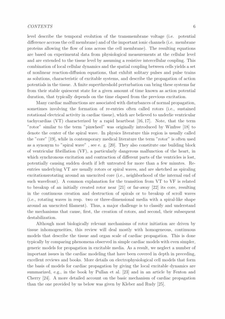
bulk of the heart. In Figure 1 the main parts of the heart are identified.
Figure 1. Explanatory sketch of the different parts of heart, including the four
electrically active chambers: two atria and two ventricles; and the main elements of the
heart’s blood circulation system, including most relevant arteries and veins. Reprinted
from the free open access book [39].
The heart is composed of cardiac muscle with intervening connective tissue, blood
vessels and nerves. Cardiac tissue is divided into three layers called endocardium,
myocardium and epicardium. The endocardium and epicardium are the internal and
external layers, respectively. In the middle lies the myocardium, thicker than the
former. Between the endocardium and myocardium is the subendocardial layer, where
the impulse-conducting system (Purkinje fibers) is located.
2.2. The cardiac myocytes
Cardiac cells are called myocytes, having a length of 80 − 100µm and a diameter
of 10 − 20µm. Each of these cells is separated from the extracellullar space by a
phospholipid bilayer membrane. This membrane presents selective permitivity, allowing
CONTENTS 9
some ions (Na+, K+, Ca2+, etc) to flow between the extracellular and intracellular
media through a set of specific ion channels. The resulting charge imbalance produces a
transmembrane potential difference, whose evolution is governed by the balance between
the electrical and chemical gradients across the membrane of the cell. The potential at
which chemical and electrical forces are in equilibrium is called the reversal or Nernst
potential, and is specific to each ion. The potential at which the cell is at rest is known
as the resting potential, and in cardiac cells its value is typically around −85 mV. If a
sufficiently large stimulus is given to the cell, the transmembrane potential rises above
a threshold potential and an active response occurs, known as an action potential. The
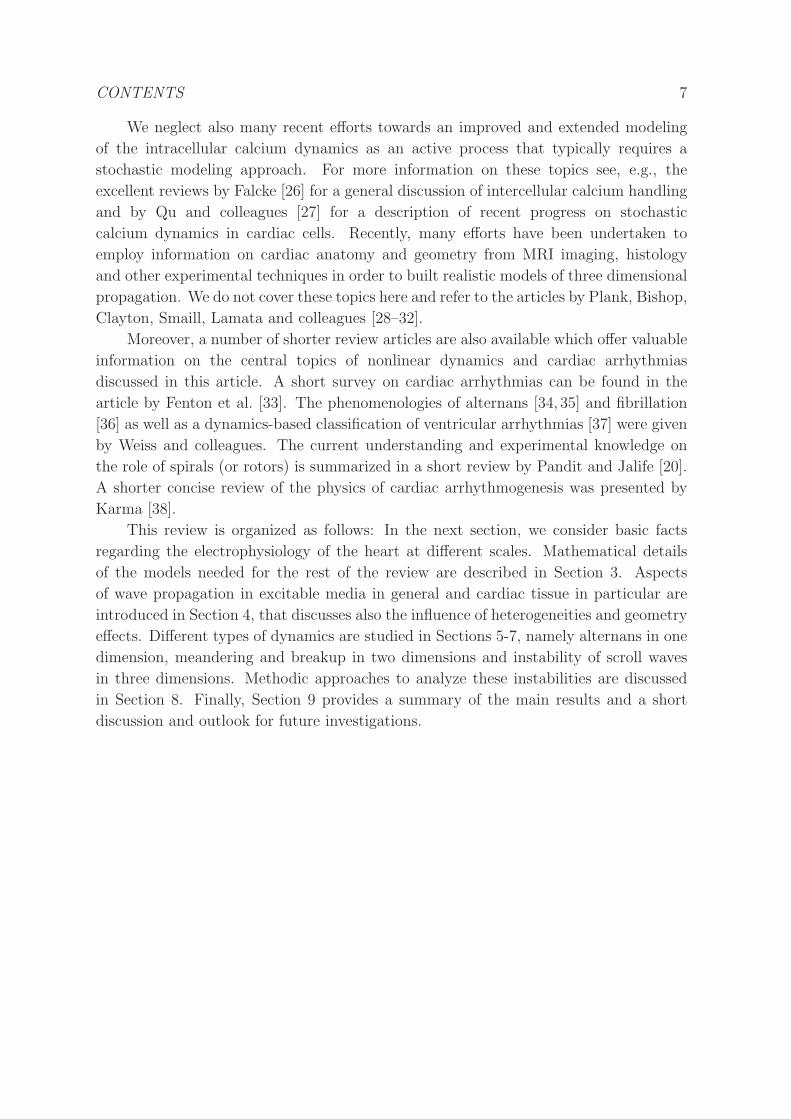
amplitude of a cardiac action potential is of the order of 130 mV.
Figure 2. Sketch of a typical action potential in a ventricular myocyte. Phases and
ion currents responsible for the action potential: sharp increase due to sodium influx
(0), rapid decrease due to potassium outflux (1), balance currents and plateu phase
(2), end of calcium influx (3) and return to the resting potential (4).
In Figure 2, a typical time evolution of the transmembrane potential is shown,
resulting in an action potential with different phases. Phase 0 is characterized by a sharp
stroke due to rapid influx of sodium ions. During phase 1 there is a rapid decrease in the
membrane potential due to a fast outward potassium current. This is then balanced by
the inward Ca2+ currents giving rise to the characteristic plateau of phase 2. Finally, in
phase 3 the calcium currents cease and the membrane returns to its resting potential,
or phase 4, due to a slow outward potassium current. In summary, during phase 0
there is a depolarization (i.e., change in membrane potential from negative to positive
values) of the cell membrane while phase 3 corresponds to repolarization (i.e., change
in membrane potential that returns it to a negative value) of the membrane.
Myocytes are connected to each other by means of intercalated discs, which are
responsible of the mechanical and electrical coupling among cells. The latter is produced
through gap junctions (i.e., pipe-like channels that permit the flow of ions from one cell
to another). This results in the propagation of the action potential in tissue, giving rise
to an excitation wave, with a propagation speed characteristic of the type of cardiac
CONTENTS 10
tissue. Gap junctions are located at the longitudinal ends of the myocytes, that are
bundled in cardiac fibers along which the propagation speed is faster. Thus, cardiac
action potential propagation is both discrete and anisotropic.
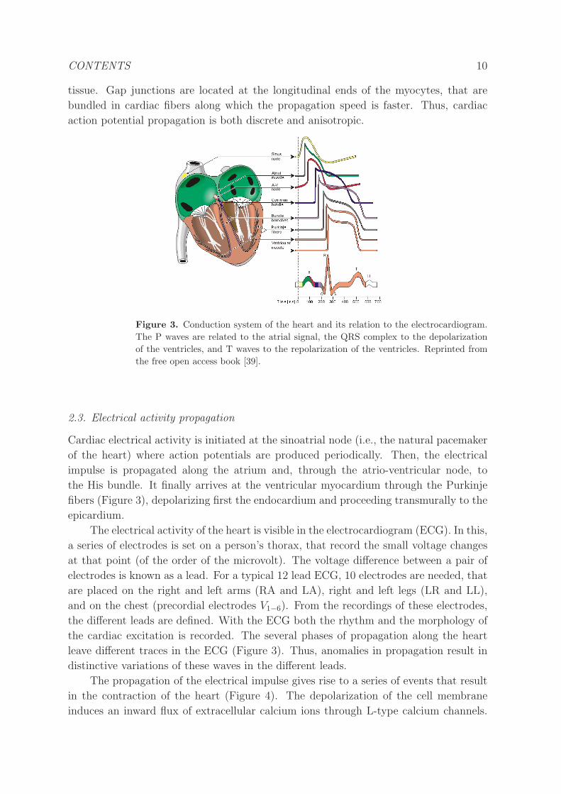
Figure 3. Conduction system of the heart and its relation to the electrocardiogram.
The P waves are related to the atrial signal, the QRS complex to the depolarization
of the ventricles, and T waves to the repolarization of the ventricles. Reprinted from
the free open access book [39].
2.3. Electrical activity propagation
Cardiac electrical activity is initiated at the sinoatrial node (i.e., the natural pacemaker
of the heart) where action potentials are produced periodically. Then, the electrical
impulse is propagated along the atrium and, through the atrio-ventricular node, to
the His bundle. It finally arrives at the ventricular myocardium through the Purkinje
fibers (Figure 3), depolarizing first the endocardium and proceeding transmurally to the
epicardium.
The electrical activity of the heart is visible in the electrocardiogram (ECG). In this,
a series of electrodes is set on a person’s thorax, that record the small voltage changes
at that point (of the order of the microvolt). The voltage difference between a pair of
electrodes is known as a lead. For a typical 12 lead ECG, 10 electrodes are needed, that
are placed on the right and left arms (RA and LA), right and left legs (LR and LL),
and on the chest (precordial electrodes V1−6). From the recordings of these electrodes,
the different leads are defined. With the ECG both the rhythm and the morphology of
the cardiac excitation is recorded. The several phases of propagation along the heart
leave different traces in the ECG (Figure 3). Thus, anomalies in propagation result in
distinctive variations of these waves in the different leads.
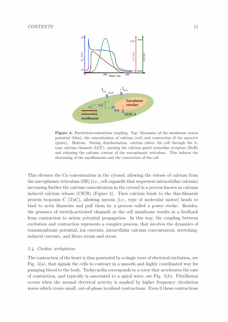
The propagation of the electrical impulse gives rise to a series of events that result
in the contraction of the heart (Figure 4). The depolarization of the cell membrane
induces an inward flux of extracellular calcium ions through L-type calcium channels.
CONTENTS 11
Figure 4. Excitation-contraction coupling. Top: Dynamics of the membrane action
potential (blue), the concentration of calcium (red) and contraction of the myocyte
(green). Bottom: During depolarization, calcium enters the cell through the L-
type calcium channels (LCC), opening the calcium gated ryanodine receptors (RyR)
and releasing the calcium content of the sarcoplasmic reticulum. This induces the
shortening of the myofilaments and the contraction of the cell.
This elevates the Ca concentration in the cytosol, allowing the release of calcium from
the sarcoplasmic reticulum (SR) (i.e., cell organelle that sequesters intracelullar calcium)
increasing further the calcium concentration in the cytosol in a process known as calcium
induced calcium release (CICR) (Figure 4). Then calcium binds to the thin-filament
protein troponin C (TnC), allowing myosin (i.e., type of molecular motor) heads to
bind to actin filaments and pull them by a process called a power stroke. Besides,
the presence of stretch-activated channels at the cell membrane results in a feedback
from contraction to action potential propagation. In this way, the coupling between
excitation and contraction represents a complex process, that involves the dynamics of
transmembrane potential, ion currents, intracellular calcium concentration, stretching-
induced currents, and fibers strain and stress.
2.4. Cardiac arrhytmias
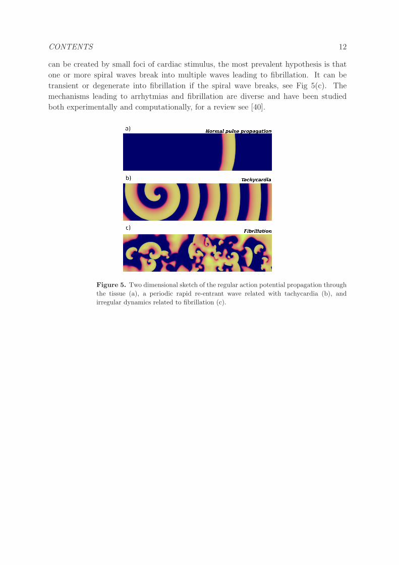
The contraction of the heart is thus generated by a single wave of electrical excitation, see
Fig. 5(a), that signals the cells to contract in a smooth and highly coordinated way for
pumping blood to the body. Tachycardia corresponds to a rotor that accelerates the rate
of contraction, and typically is associated to a spiral wave, see Fig. 5(b). Fibrillation
occurs when the normal electrical activity is masked by higher frequency circulation
waves which create small, out-of-phase localized contractions. Even if these contractions
CONTENTS 12
can be created by small foci of cardiac stimulus, the most prevalent hypothesis is that
one or more spiral waves break into multiple waves leading to fibrillation. It can be
transient or degenerate into fibrillation if the spiral wave breaks, see Fig 5(c). The
mechanisms leading to arrhytmias and fibrillation are diverse and have been studied
both experimentally and computationally, for a review see [40].
Figure 5. Two dimensional sketch of the regular action potential propagation through
the tissue (a), a periodic rapid re-entrant wave related with tachycardia (b), and
irregular dynamics related to fibrillation (c).
CONTENTS 13
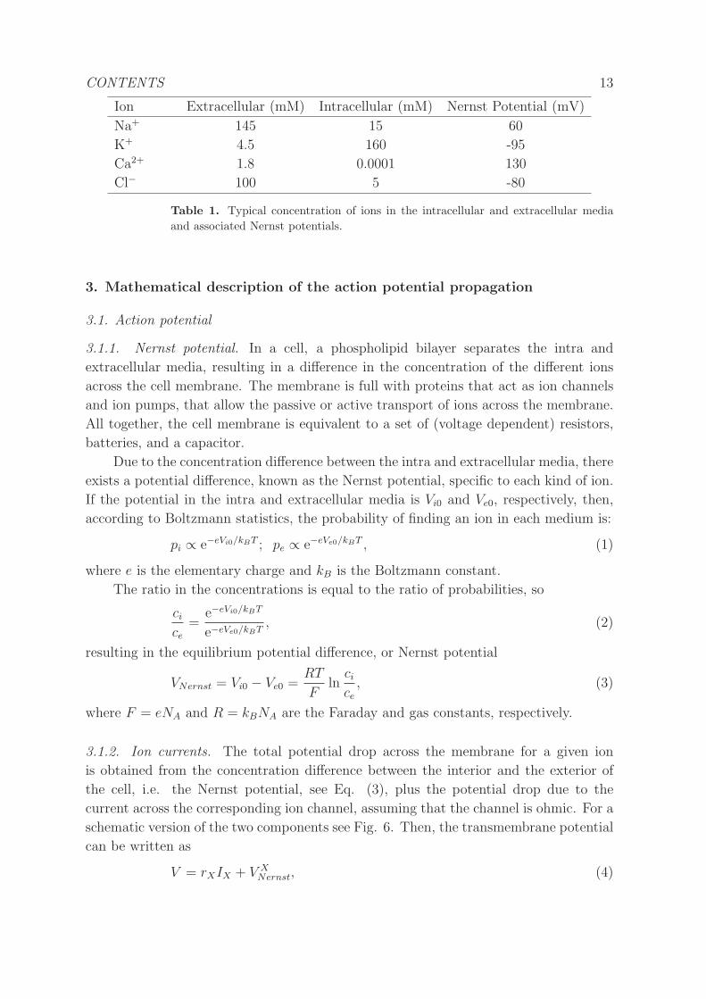
Ion Extracellular (mM) Intracellular (mM) Nernst Potential (mV)
Na+ 145 15 60
K+ 4.5 160 -95
Ca2+ 1.8 0.0001 130
Cl− 100 5 -80
Table 1. Typical concentration of ions in the intracellular and extracellular media
and associated Nernst potentials.
3. Mathematical description of the action potential propagation
3.1. Action potential
3.1.1. Nernst potential. In a cell, a phospholipid bilayer separates the intra and
extracellular media, resulting in a difference in the concentration of the different ions
across the cell membrane. The membrane is full with proteins that act as ion channels
and ion pumps, that allow the passive or active transport of ions across the membrane.
All together, the cell membrane is equivalent to a set of (voltage dependent) resistors,
batteries, and a capacitor.
Due to the concentration difference between the intra and extracellular media, there
exists a potential difference, known as the Nernst potential, specific to each kind of ion.
If the potential in the intra and extracellular media is Vi0 and Ve0, respectively, then,
according to Boltzmann statistics, the probability of finding an ion in each medium is:
pi ∝ e−eVi0/kBT ; pe ∝ e−eVe0/kBT , (1)
where e is the elementary charge and kB is the Boltzmann constant.
The ratio in the concentrations is equal to the ratio of probabilities, so
cice
=e−eVi0/kBT
e−eVe0/kBT, (2)
resulting in the equilibrium potential difference, or Nernst potential
VNernst = Vi0 − Ve0 =RT
Fln
cice, (3)
where F = eNA and R = kBNA are the Faraday and gas constants, respectively.
3.1.2. Ion currents. The total potential drop across the membrane for a given ion
is obtained from the concentration difference between the interior and the exterior of
the cell, i.e. the Nernst potential, see Eq. (3), plus the potential drop due to the
current across the corresponding ion channel, assuming that the channel is ohmic. For a
schematic version of the two components see Fig. 6. Then, the transmembrane potential
can be written as
V = rXIX + V XNernst, (4)
CONTENTS 14
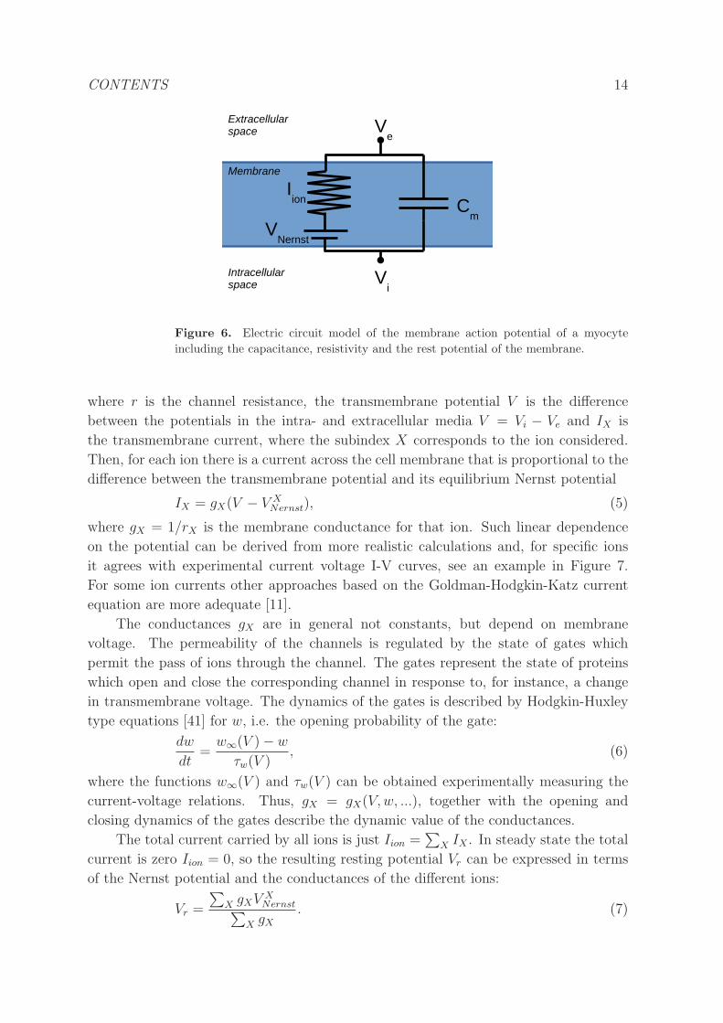
Figure 6. Electric circuit model of the membrane action potential of a myocyte
including the capacitance, resistivity and the rest potential of the membrane.
where r is the channel resistance, the transmembrane potential V is the difference
between the potentials in the intra- and extracellular media V = Vi − Ve and IX is
the transmembrane current, where the subindex X corresponds to the ion considered.
Then, for each ion there is a current across the cell membrane that is proportional to the
difference between the transmembrane potential and its equilibrium Nernst potential
IX = gX(V − V XNernst), (5)
where gX = 1/rX is the membrane conductance for that ion. Such linear dependence
on the potential can be derived from more realistic calculations and, for specific ions
it agrees with experimental current voltage I-V curves, see an example in Figure 7.
For some ion currents other approaches based on the Goldman-Hodgkin-Katz current
equation are more adequate [11].
The conductances gX are in general not constants, but depend on membrane
voltage. The permeability of the channels is regulated by the state of gates which
permit the pass of ions through the channel. The gates represent the state of proteins
which open and close the corresponding channel in response to, for instance, a change
in transmembrane voltage. The dynamics of the gates is described by Hodgkin-Huxley
type equations [41] for w, i.e. the opening probability of the gate:
dw
dt=
w∞(V )− w
τw(V ), (6)
where the functions w∞(V ) and τw(V ) can be obtained experimentally measuring the
current-voltage relations. Thus, gX = gX(V,w, ...), together with the opening and
closing dynamics of the gates describe the dynamic value of the conductances.
The total current carried by all ions is just Iion =∑
X IX . In steady state the total
current is zero Iion = 0, so the resulting resting potential Vr can be expressed in terms
of the Nernst potential and the conductances of the different ions:
Vr =
∑
X gXVXNernst
∑
X gX. (7)
CONTENTS 15
-80 -60 -40 -20 0 20 40V / mV
-2
-1,5
-1
-0,5
0
0,5
1
I / n
A 0 10 20 30 40 50V / mV
-1
-0,5
0
0,5
I / n
A
(a)(b)
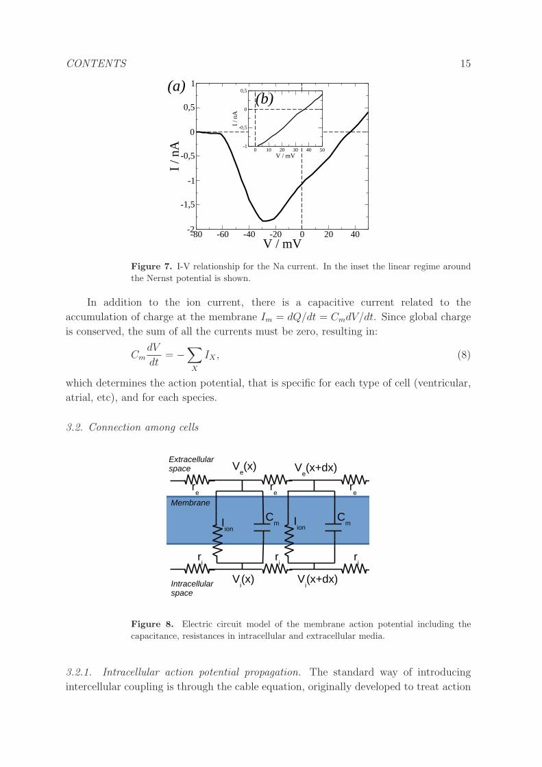
Figure 7. I-V relationship for the Na current. In the inset the linear regime around
the Nernst potential is shown.
In addition to the ion current, there is a capacitive current related to the
accumulation of charge at the membrane Im = dQ/dt = CmdV/dt. Since global charge
is conserved, the sum of all the currents must be zero, resulting in:
CmdV
dt= −
∑
X
IX , (8)
which determines the action potential, that is specific for each type of cell (ventricular,
atrial, etc), and for each species.
3.2. Connection among cells
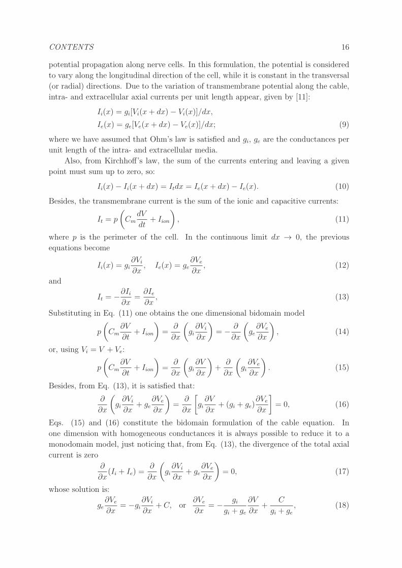
Figure 8. Electric circuit model of the membrane action potential including the
capacitance, resistances in intracellular and extracellular media.
3.2.1. Intracellular action potential propagation. The standard way of introducing
intercellular coupling is through the cable equation, originally developed to treat action
CONTENTS 16
potential propagation along nerve cells. In this formulation, the potential is considered
to vary along the longitudinal direction of the cell, while it is constant in the transversal
(or radial) directions. Due to the variation of transmembrane potential along the cable,
intra- and extracellular axial currents per unit length appear, given by [11]:
Ii(x) = gi[Vi(x+ dx)− Vi(x)]/dx,
Ie(x) = ge[Ve(x+ dx)− Ve(x)]/dx; (9)
where we have assumed that Ohm’s law is satisfied and gi, ge are the conductances per
unit length of the intra- and extracellular media.
Also, from Kirchhoff’s law, the sum of the currents entering and leaving a given
point must sum up to zero, so:
Ii(x)− Ii(x+ dx) = Itdx = Ie(x+ dx)− Ie(x). (10)
Besides, the transmembrane current is the sum of the ionic and capacitive currents:
It = p
(
CmdV
dt+ Iion
)
, (11)
where p is the perimeter of the cell. In the continuous limit dx → 0, the previous
equations become
Ii(x) = gi∂Vi
∂x, Ie(x) = ge
∂Ve
∂x, (12)
and
It = −∂Ii∂x
=∂Ie∂x
, (13)
Substituting in Eq. (11) one obtains the one dimensional bidomain model
p
(
Cm∂V
∂t+ Iion
)
=∂
∂x
(
gi∂Vi
∂x
)
= − ∂
∂x
(
ge∂Ve
∂x
)
, (14)
or, using Vi = V + Ve:
p
(
Cm∂V
∂t+ Iion
)
=∂
∂x
(
gi∂V
∂x
)
+∂
∂x
(
gi∂Ve
∂x
)
. (15)
Besides, from Eq. (13), it is satisfied that:
∂
∂x
(
gi∂Vi
∂x+ ge
∂Ve
∂x
)
=∂
∂x
[
gi∂V
∂x+ (gi + ge)
∂Ve
∂x
]
= 0, (16)
Eqs. (15) and (16) constitute the bidomain formulation of the cable equation. In
one dimension with homogeneous conductances it is always possible to reduce it to a
monodomain model, just noticing that, from Eq. (13), the divergence of the total axial
current is zero
∂
∂x(Ii + Ie) =
∂
∂x
(
gi∂Vi
∂x+ ge
∂Ve
∂x
)
= 0, (17)
whose solution is:
ge∂Ve
∂x= −gi
∂Vi
∂x+ C, or
∂Ve
∂x= − gi
gi + ge
∂V
∂x+
C
gi + ge, (18)
CONTENTS 17
from which we obtain the monodomain cable equation:
p
(
Cm∂V
∂t+ Iion
)
=∂
∂x
(
gigegi + ge
∂V
∂x
)
, (19)
where we can define an effective conductante geff = gige/(gi+ge), which is the harmonic
mean of the conductances1
geff=
1
gi+
1
ge, (20)
which ensures a null conductance if any of the conductances is zero [11].
3.2.2. Intercellular action potential propagation. So far, the equations derived above
are valid for propagation in a single cardiomyocyte. For the modeling of tissue one has
to consider cardiac cells coupled through gap junctions, and different approaches can be
employed.
Continuum model. In the continuum model one has to solve the cable equation in each
cardiomyocyte and impose boundary conditions at the gap junctional space, such that
gi∂Vi
∂x(x = x−
j ) = gi∂Vi
∂x(x = x+
j ) = gjVj, (21)
where gj is the gap junction conductance, x+j and x−
j represent the positions of the right
and left sides of the junction, and Vj = Vi(x = x+j ) − Vi(x = x−
j ) is the intracellular
voltage drop across the gap junction. A simpler formulation is to consider the continuum
cable equation (19), but for an effective conductance geff that is an average of the
conductances at the intracellular medium and gap junctional spaces in a similar way
than the harmonic mean employed in Eq. (20) and obtained from a homogenization
approach [42]. In any of these cases, the difference between a continuum and a discrete
description only appears when studying the effects of propagation failure [43], typical
for low conductivities and determined by the interplay between the properties of the
action potential of the myocytes and structural properties of the tissue.
Isopotential model. An alternative approach is to assume an isopotential model, in
which the whole cell is at the same potential and the potential drops occur only at
the gap junction resistances. Then, one should consider the discretized version of the
continuum equations, with a spatial step equal to the size of the cell dx ≃ 100µm, and
gi ≡ gj, the gap junction conductance. Such a model is convenient when considering the
effects of the time and voltage dependence of the gap junction conductances. In general
terms gj = gj(Vj, t), where Vj is the transjunctional potential, so Vj = V n+1i − V n
i is the
difference in intracellular potential of the two cells joined by the gap junction. The gap
junction itself behaves as a gate, so
dgjdt
=gss(Vj)− gj
τj(Vj)(22)
CONTENTS 18
with the steady state conductance and time constant depending on the intercellular
potential, such that
gss = gmin +gmax − gmin
1 + exp [A(Vj − V1/2)], τj(Vj) = τj0e
−Vj/Vτ . (23)
Typical values are V1/2 ∼ 40 − 60 mV, Vτ ∼ 15 mV, and τj0 ∼ 100s [44]. For typical
wave speeds of 50-70 cm/s and durations of the upstroke of ∼ 3 − 5 ms the width of
the front of the depolarization pulse is ∼ 0.15 − 0.45cm, corresponding to 15-45 cells.
Given the upstroke voltage difference of ∼ 100mV, then the voltage difference between
cells is, at most, ∼ 6 − 7mV. Thus, under normal conditions, the dynamics of the
gap junction conductances does not seem to play a role, and one can assume it to be
constant. However, in some cardiac diseases there is a reduction or redistribution of the
protein molecules forming gap junction channels, from intercalated disks to lateral cell
borders [45]. The resulting gap junction and connexin expression remodeling [46, 47]
reduces conduction velocity and enhances anisotropy in diseased myocardium [48].
3.2.3. 3D formulation. A generalization of the cable equation to three dimensional
tissue can be made, assuming that cardiac tissue is composed of two media, so at each
point of space we can define intracellular and extracellular potentials. Then, assuming
Ohm’s law, we can write the currents as Je = σe∇Ve, Ji = σi∇Vi, where σi(x) and
σe(x) are the conductances of the intra- and extracellular media, that in this case are
assumed to be of tensorial character, so they define directions where propagation is
faster (or slower) and depend on the distribution of cardiac fibers in tissue. Here,
implicitly we are assuming that these conductances are average values over gap junctions,
inhomogeneities, etc. Again, applying Kirchhoff’s law, we obtain the bidomain model
for three-dimensional tissue, which are the equivalent of Eqs. (14) and (17):
χ
(
Cm∂V
∂t+ Iion
)
= ∇ · (σi∇Vi) = −∇ · (σe∇Ve), (24)
∇ · (σi∇Vi + σe∇Ve) = 0; (25)
where now χ is the ratio of surface to cell volume. In the case when σi = λσe, so the
anisotropy ratios are the same in the intracellular and extracellular media (which is
not the case in cardiac tissue), the above description can be reduced to a monodomain
equation for the transmembrane potential. In effect, in this case
∇ · (σe∇Ve) = − λ
1 + λ∇ · (σe∇V ), (26)
so we obtain the monodomain equation:
χ
(
Cm∂V
∂t+ Iion
)
=λ
1 + λ∇ · (σe∇V ). (27)
Then, the propagation of the transmembrane potential is described by the equation:
∂V
∂t= − Iion
Cm
+∇ · (D∇V ), (28)
CONTENTS 19
where typical values of the membrane capacitance are Cm ∼ 1 − 10µF/cm2, varying
for different types of cells or different species [49]. The diffusion coefficient D ∼ 0.001
cm2/ms is derived from the resistivity between cells, and the cell capacitance and surface
to volume ratio [11]. Resistivity and surface to volume ratio, usually obtained from an
approximation of a cardiac cell by a cylinder, may also change from cell to cell.
For the rest of the review we will consider the monodomain description of cardiac
tissue propagation Eq. (28). Although this is not a correct description for two and
three-dimensional tissue [50], since the intracellular medium is more anisotropic than
the extracellular medium, it is usually a sufficient description of action potential
propagation in most situations. A relevant exception is the case of defibrillation, where
a bidomain description is required [51,52]. The injection of current into resting cardiac
tissue produces the formation of virtual electrodes, that are thought to be behind
the mechanism by which an external electric shock is able to annihilate reentrant
waves. Such virtual electrodes are virtual cathodes and anodes resulting from unequal
anisotropy ratios of the intracellular and extracellular spaces of the cardiac [51–53] or
from the borders of non-conducting heterogeneities [54, 55].
3.3. Ionic models
Ion currents across the ion channels at the cell membrane are governed by highly
nonlinear processes. There are different types of active cells in the heart and the explicit
form of the total current Iion depends on the type of cell and species [33].
• Ventricular myocytes. The action potential dynamics of ventricular myocytes has
been amply studied. There is a large list of ventricle cell models [33], which
are developed for different type of species, from mice or rabbits to dogs and
humans. The ventricles are the largest chambers of the heart and where electrical
discoordination becomes more dangerous [56]. Furthermore the thickness of the
ventricular walls makes it necessary to consider the three-dimensional structure of
the tissue.
• Atrial myocytes. The models for atrial cells are characterized by a short action
potential due to the reduced calcium current with respect to ventricular myocytes.
There are several models for the action potential of atrial cells, for a comparison
between two of the latest models in human tissue see [57].
• Cells forming the sinoatrial node. The regular activity of the heart is initiated by
this specialized population of cardiac cells. Their membrane potential oscillates
periodically [58], generating electrical oscillatory signals. A detailed comparison of
all the numerical models of automaticity has been recently presented [59].
• Purkinje fibers. The first models of cardiac cells were derived for this type of
cells [60]. The network of the Purkinje fibers produces a fast conduction pathway
to transmit electrical excitation from the atria into the ventricles [61]. The action
potentials of the myocytes at the Purkinje fibers present characteristic features:
CONTENTS 20
the velocity of propagation is faster than in other types of cardiac cells, and the
action potential duration is longer [61]. These cells can also present automaticity
and produce oscillations. For a review of several models of the Purkinje fibers cells
see [62].
For concreteness, in this review we focus in models of ventricular cardiac tissue. A
full description of all the possible ion currents, together with the dynamics of the ion
channel gates, is complex and produces models with a large number of equations. In
contrast, generic models try to reproduce the main properties of such ion currents with a
reduced number of parameters. In this section, we classify the models employed for the
study of wave instabilities in cardiac tissue in three classes. First, we consider realistic
ionic models that describe in detail several ion currents across the cell membrane.
Second, we study simple cardiac models that fit the main characteristic experimental
features of the action potential into simpler formulations. Finally, we consider generic
models of excitable media.
3.3.1. Detailed electrophysiological models. Electrophysiological detailed models [30]
are based on direct experimental observations from voltage and patch clamp studies.
Typically, these models include many Hodgkin-Huxley type equations [41] to describe
individual ion currents (IX) forming the total current Iion(V,w, pi) =∑
X IX across the
cell membrane [63]. Modern ionic models also describe the changes of concentrations
of all major ions inside cardiac cells, and generally consist of anywhere between 10 and
60 equations [64, 65]. The quantitative descriptions of ion currents in cardiac tissue
are continually being revised, and there is not general agreement on the best model
for all circumstances [66]. Detailed models are adequate to numerically explore the
effects of different drugs in the propagation properties of the action potential [67]. The
nonlinear terms are typically stiff so adaptive methods are usually required to obtain
fast integration speeds [68, 69].
Below, we present some detailed electrophysiological models that have been amply
used in studies of cardiac wave propagation.
• Beeler-Reuter model. One of the first models of action potential in ventricular
myocytes is the Beeler-Reuter model [70]. It was the first ionic model used
to simulate spatio-temporal propagation in two dimensions [71]. It reproduces
important experimental phenomena by the use of four individual ion currents
in terms of Hodgkin-Huxley type equations. The total current for this model is
Iion = INa + ICa + Ix1 + IK1, where the corresponding ion currents are:
INa = (GNam3hj +GNaC)(V − ENa),
ICa = Gsdf(V − Esi),
Ix1 = x10.8e0.04(V+77) − 1
e0.04(V+35),
IK1 = 0.35
(
4e0.04(V+85) − 1
e0.08(V+53) + e0.04(V+53)+ 0.2
V + 23
1− e−0.04(V+23)
)
, (29)
CONTENTS 21
where INa is the fast inward Na+ current, adapted from the sodium activation
parameter determined for squid axon by Hodgkin and Huxley [41]; ICa is the slow
inward Ca2+ current, which follows the same functional form; Ix1 is the time-
activated outward current and IK1is the time-independent K+ outward current.
The dependence on the membrane voltage of the latter two currents is chosen to
match current-voltage relations seen in myocardium, and they produce a reasonable
plateau and repolarization and it was originally introduced for purkinje fibers
modeling in [72]. The values ENa, Esi are reversal potentials and m, h, j, d, f
and x1 are gating variables, whose dynamics can be modeled as
dwi
dt= (wi∞ − wi)/τwi
, (30)
where wi represents any of the gating variables, and wi∞ and τwi, which depend on
V , are the steady state value and the relaxation time constant for the corresponding
variable, see Eq. (6). The shape of the action potential can be seen in Fig.9(a) with
standard values of the parameters of the model.
This model was posteriorly modified giving rise to several versions of the model. A
calcium speedup was introduced in [71] to suppress spiral wave breakup present in
the original equations giving rise to the modified Beeler-Reuter model.
• Luo-Rudy model. Multitude of results regarding ventricular tissue have been
illustrated with the Luo-Rudy phase 1 (LR1) model [64]. It describes the biophysical
mechanism of generation of action potential in cardiac guinea pig cells by a relatively
small number of state variables and was widely used to study wave propagation in
2D and 3D cardiac tissue [73, 74]. This model speeds up the opening and closing
rate coefficients for the sodium current from Beeler-Reuter model, see Eqs. (29),
and adds three new currents following the classical Hodgkin and Huxley description.
The representation of the total current is Iion = INa + Isi + IK + IK1 + IKp + Ib,
where the corresponding currents are:
INa = GNam3hj(V − ENa),
Isi = Gsidf(V − Esi),
IK = GKxx1(V − EK),
IK1= GK1
K1∞(V − EK1),
IKp = GKpKp(V − EKp),
Ib = Gb(V − Eb); (31)
where INa is the fast Na+ current, Isi is the slow inward Ca2+ current, IK is the slow
outward K+ current, IK1is the time-independent K+ current, IKp is the plateau
K+ current, and Ib is a background current with constant conductance. The values
ENa, Esi, EK , EK1, EKp and Eb are the reversal potentials and m, h, j, d, f and x
are again gating variables, whose dynamics can be modeled by Eq. (30).
The sodium conductance GNa controls the speed of the waves [75] and in a
general sense the excitability of the tissue, and Gsi is responsible for the front-
tail interaction between the pulses.
CONTENTS 22
An extension of this model is the Luo-Rudy phase 2 (LR2) model that includes a
more detailed description of intracellular Ca2+ [76].
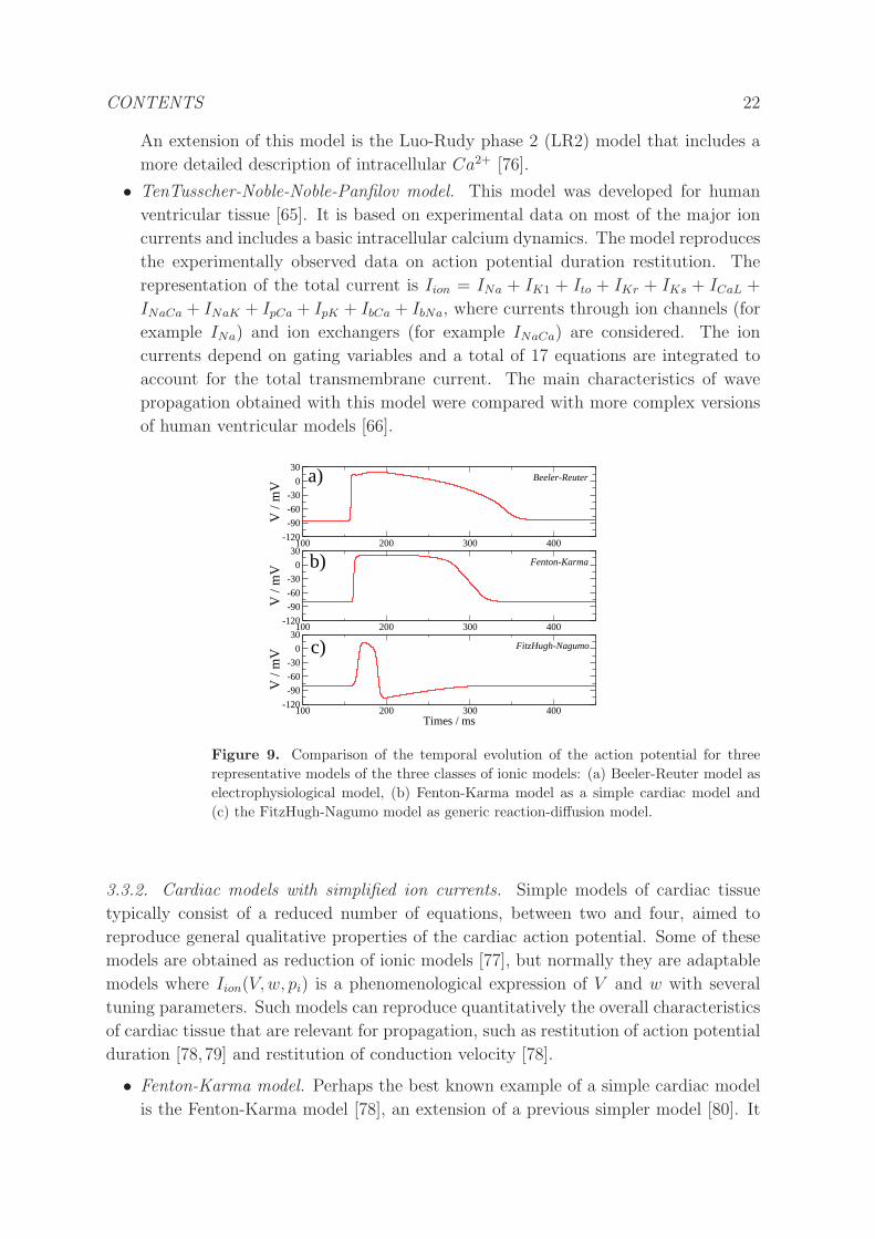
• TenTusscher-Noble-Noble-Panfilov model. This model was developed for human
ventricular tissue [65]. It is based on experimental data on most of the major ion
currents and includes a basic intracellular calcium dynamics. The model reproduces
the experimentally observed data on action potential duration restitution. The
representation of the total current is Iion = INa + IK1 + Ito + IKr + IKs + ICaL +
INaCa + INaK + IpCa + IpK + IbCa + IbNa, where currents through ion channels (for
example INa) and ion exchangers (for example INaCa) are considered. The ion
currents depend on gating variables and a total of 17 equations are integrated to
account for the total transmembrane current. The main characteristics of wave
propagation obtained with this model were compared with more complex versions
of human ventricular models [66].
100 200 300 400Times / ms
-120
-90
-60
-30
0
30
V /
mV
100 200 300 400-120
-90
-60
-30
0
30
V /
mV
100 200 300 400-120
-90
-60
-30
0
30
V /
mV
FitzHugh-Nagumo
Fenton-Karma
Beeler-Reutera)
b)
c)
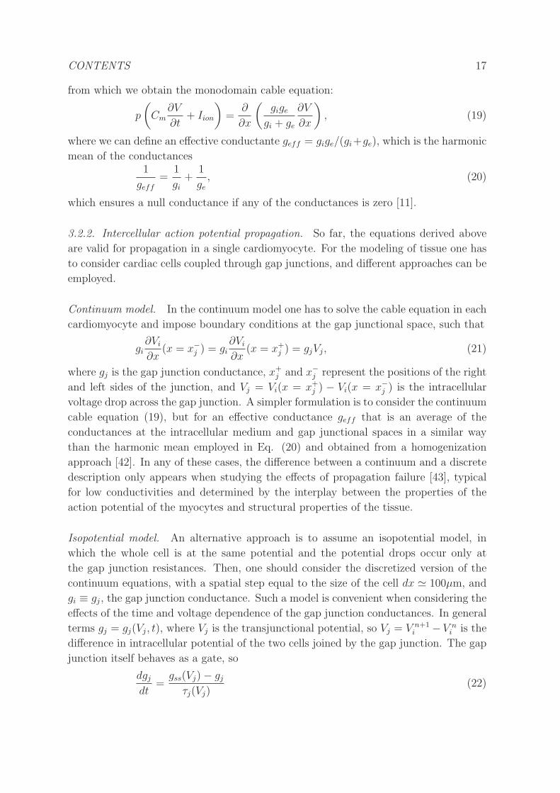
Figure 9. Comparison of the temporal evolution of the action potential for three
representative models of the three classes of ionic models: (a) Beeler-Reuter model as
electrophysiological model, (b) Fenton-Karma model as a simple cardiac model and
(c) the FitzHugh-Nagumo model as generic reaction-diffusion model.
3.3.2. Cardiac models with simplified ion currents. Simple models of cardiac tissue
typically consist of a reduced number of equations, between two and four, aimed to
reproduce general qualitative properties of the cardiac action potential. Some of these
models are obtained as reduction of ionic models [77], but normally they are adaptable
models where Iion(V,w, pi) is a phenomenological expression of V and w with several
tuning parameters. Such models can reproduce quantitatively the overall characteristics
of cardiac tissue that are relevant for propagation, such as restitution of action potential
duration [78,79] and restitution of conduction velocity [78].
• Fenton-Karma model. Perhaps the best known example of a simple cardiac model
is the Fenton-Karma model [78], an extension of a previous simpler model [80]. It
CONTENTS 23
consists of the usual cable equation:
∂v
∂t= − Ifi + Iso + Isi
Cm
+∇ · (D∇v), (32)
for a renormalized variable v. From this the transmembrane potential can be
approximated by V = (100v − 80)mV . The three phenomenological currents read:
Ifi = − up(v − Vc)(1− v)/τd,
Iso = v(1− p)/τo + p/τr,
Isi = − w
1 + tanh[k(v − V sic )]
/(2τsi), (33)
mimicking fast inward sodium (Ifi), slow outward potassium (Iso) and slow inward
calcium (Isi) currents. The variables u and w are gating variables which are used to
regulate inactivation of the fast inward and slow inward currents. Their evolution
depends on the transmembrane potential:
du
dt= (1− p)(1− u)/τ−u (v)− pu/τ+u ,
dw
dt= (1− p)(1− w)/τ−w − pw/τ+w ; (34)
where
p =
1 if v ≥ Vc,
0 if v < Vc,(35)
and
τ−u (v) = (1− q)τ−u1 + qτ−u2 with q =
1 if v ≥ Vv,
0 if v < Vv.(36)
The gate variables u and w are related respectively to the product of the gates h
and j of the sodium current, as well as to the gate f controlling the inactivation and
reactivation of the calcium current, in the more elaborated models of section (3.3.1).
Expressions (33) are not based on physical models of realistic ion currents, however
the flexibility of the functions Eqs. (34) permits the tunning of the parameters to
reproduce different propagation properties of experiments or other more realistic
models. Figure 9(b) shows an example of the action potential with this model.
The Fenton-Karma model with different parameter values has been employed to
study diverse types of instabilities in cardiac tissue [40]. More realistic action
potential shapes have been obtained with the extension of this model by an
additional equation [81,82].
• Aliev-Panfilov model. This is another frequently used model with simplified kinetics
[79]. It does not describe ion currents but the model is formed by nonlinear functions
which may be tuned to reproduce pulse shape and the restitution properties of the
canine myocardium with good precision. The model consists of just two equations
∂v
∂t= − p0v(v − p3)(v − 1)− vw +∇ · (D∇v),
∂w
∂t=
(
ǫ0 +p1w
v + p2
)
(w − p0v(v − p3 − 1)) (37)
CONTENTS 24
where v is a renormalized transmembrane potential, related to the physiological
one by V = 100v− 80 mV . The parameters ǫ0, p1 and p2 specify the scale between
v and the control variable w. The parameters p0 and p3 determine the shape of the
cubic function which controls the action potential dynamics. This model can also
be considered an extension of the FitzHugh-Nagumo model, discussed in the next
section.
Besides these two models, there is a collection of reduced models created with the
same spirit as the ones here described. Other two-variable cardiac models were employed
for the incipient simulations of cardiac arrhythmias [83] and the first descriptions of
spiral breakup [84].
3.3.3. Generic reaction-diffusion models. Generic excitable media can be described by
a system of two coupled reaction-diffusion equations:
∂v
∂t= ∇ · (D∇v) + I(v, w, pi),
∂w
∂t= R(v, w, pi); (38)
where v corresponds to a scaled transmembrane potential V .
These generic models of excitable media are not derived from physiological data
and some properties of the waves often differ from waves of transmembrane potential in
physiologically realistic models. Since they do not aim at quantitative agreement, it is
usual to consider the functions I(v, w, pi) and R(v, w, pi) as simple as possible [85, 86].
A simple model should contain at least a stable equilibrium state, a threshold for wave
triggering and a refractory period [87].
The main advantage of these models is their simplicity, together with their ability
to reproduce general qualitative properties of cardiac excitation, such as generation and
propagation of a pulse, refractory properties, dispersion relations, etc. They are specially
appropriate to study features of cardiac wave propagation that are generic to a whole
range of excitable media. Besides, due to their simplicity, they allow the implementation
of effective numerical solvers and in some cases (or in some limits) they are amenable to
analytic treatment. For historical and practical reasons, here we consider three examples
of generic models:
• FitzHugh-Nagumo model. This historical model was derived in the 60s [85, 88]. It
reproduces the plateau observed in cardiac cells which was absent in the Hodgkin-
Huxley model of the nerve impulse [63]. The specific form of the reaction terms
is:
I(v, w, pi) =1
ǫ
(
v − v3
3− w
)
,
R(v, w, pi) = v + p1 − p2w; (39)
where the parameters p1 and p2 specify the inhibitor kinetics. The small parameter
ǫ is the ratio of the temporal scales between v and w. The evolution of the model
CONTENTS 25
is shown in Fig. 9(c) in comparison with more realistic description of the action
potential. The action potential is shorter than the other type of models because of
the inhibitory tail produced by the second variable w.
• Barkley model. A very popular simple model for excitable media, given by [89]:
I(v, w, pi) =1
ǫv(1− v)
(
v − w + p2p1
)
,
R(v, w, pi) = v − w; (40)
where ǫ is the ratio of the temporal scales between v and w. The parameters p1and p2 specify the activator kinetics, with p2 effectively controlling the excitation
threshold of the system.
This model has been widely used for large and systematic numerical studies due to
the particularly fast numerical implementation in two [90] and three [89] dimensions.
• Bar-Eiswirth model. The Bar-Eiswirth model is an extension of the Barkley model,
introduced to study spiral breakup [91]:
I(v, w, pi) =1
ǫv(1− v)
(
v − w + p2p1
)
,
R(v, w, pi) = f(v)− w; (41)
with a different reaction function of the inhibitor:
f(v) =
0 if v < 1/3
1− 6.75v(v − 1)2 if 1/3 ≤ v ≤ 1
1 if v > 1
(42)
This function leads to inhibitor production only above a threshold value of v, giving
rise to a rich variety of patterns.
There are several other examples of generic models which are used to study wave
dynamics in excitable media. For example the Puschino model, extensively used in
incipient numerical simulations of excitable media [92], and its modification [93].
The boundary between generic and simple cardiac models is obviously diffuse and
some FitzHugh-Nagumo-like models have been modified to obtain more physiological
descriptions of the cardiac tissue by the introduction of additional temporal scales in
the model [94].
3.4. Excitation-contraction coupling
In section 2.3 we considered wave propagation in a static medium. The heart, however,
contracts, and this effect goes beyond a mere change in the geometry, since it induces a
modification of the electrical properties of tissue [95, 96]. This has been shown to have
important implications for the creation of a proarrhythmic substrate [97].
CONTENTS 26
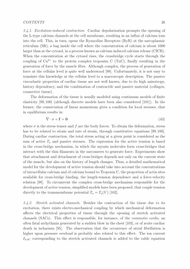
3.4.1. Excitation-induced contraction Cardiac depolarization prompts the opening of
the L-type calcium channels at the cell membrane, resulting in an influx of calcium ions
into the cell. This, in turn, opens the Ryanodine Receptors (RyR) at the sarcoplasmic
reticulum (SR), a bag inside the cell where the concentration of calcium is about 1000
larger than at the cytosol, in a process known as calcium induced calcium release (CICR).
When the concentration at the cytosol rises, the crossbridge cycle starts through the
coupling of Ca2+ to the protein complex troponim C (TnC), finally resulting in the
generation of force by the muscle fiber. Although complex, the process of generation of
force at the cellular level is quite well understood [98]. Unfortunately, it is not easy to
translate this knowledge at the cellular level to a macroscopic description. The passive
viscoelastic properties of cardiac tissue are not well known, due to its high anisotropy,
history dependency, and the combination of contractile and passive material (collagen,
connective tissue).
The deformation of the tissue is usually modeled using continuum models of finite
elasticity [99, 100] (although discrete models have been also considered [101]). In the
former, the conservation of linear momentum gives a condition for local stresses, that
in equilibrium results in:
∇ · σ + f = 0 (43)
where σ is the stress tensor and f are the body forces. To obtain the deformation, stress
has to be related to strain and rate of strain, through constitutive equations [99, 100].
During cardiac contraction, the total stress acting at a given point is considered as the
sum of active Ta and passive stresses. The expression for the active tension is based
in the cross-bridge mechanism, in which the myosin molecules form cross-bridges that
interact with the thin filaments in the sarcomeres to generate force. Experiments show
that attachment and detachment of cross-bridges depends not only on the current state
of the muscle, but also on the history of length changes. Thus, a detailed mathematical
model for the development of active tension should take into account the concentrations
of intracellular calcium and of calcium bound to Troponin C, the proportion of actin sites
available for cross-bridge binding, the length-tension dependence and a force-velocity
relation [98]. To circumvent the complex cross-bridge mechanism responsible for the
development of active tension, simplified models have been proposed, that couple tension
directly to the transmembrane potential Ta = Ta(V ) [102].
3.4.2. Stretch activated channels. Besides the contraction of the tissue due to its
excitation, there exists electro-mechanical coupling by which mechanical deformation
affects the electrical properties of tissue through the opening of stretch activated
channels (SACs). This effect is responsible, for instance, of the commotio cordis, an
often fatal arrhythmia generated by a sudden blow in the chest [103], or of acute cardiac
death in ischaemia [95]. The observation that the occurrence of atrial fibrillation is
higher upon pressure overload is probably also related to this effect. The ion current
ISAC corresponding to the stretch activated channels is added to the cable equation
CONTENTS 27
giving rise to
∂V
∂t= ∇ · (D∇V ) +
IionCm
+ISAC
Cm
. (44)
In simple formulations [104, 105] ISAC was assumed to be linearly proportional to
deformation and to the deviation of the transmembrane potential from its Nernst
equilibrium value ESAC , so
ISAC = GSAC(√C − 1)(V − ESAC). (45)
In fact, it has been observed that the conductance of this current is not a constant, but
varies with time, having an activation time of 20 ms to peak current, and then a decay
to half the peak current value in about 50 ms [106,107].
3.5. Anisotropy.
One of the main characteristics of cardiac myocytes is their elongated shape, that induces
their alignment in the tissue. A myocyte can be seen as a cylinder 100 µm long and 10-
20 µm wide. The fibers of the cell are oriented parallel to their long axis, and contract
in such direction.
The gap junctions mainly accumulate at both ends of the cylinder. In tissue, this
asymmetrical distribution of gap junctions produces a faster propagation of the action
potential along the direction parallel to the myocytes axis than perpendicularly to it,
with a 2:1 velocity ratio. More detailed models consider also the laminar order of the
cells in the tissue, introducing an additional anisotropy in the velocity of the waves,
giving rise to three different velocities with ratio 4:2:1. Such velocities correspond,
respectively, to the fiber axis, parallel to the laminar arrangement of myocytes, and
normal to the arrangement of myocytes [108].
The effect of anisotropy can be incorporated into a model of wave propagation in
cardiac tissue by the modification of the diffusion coefficient in the cable equation (28).
In the monodomain approach the diffusion tensor is usually determined by two diffusion
coefficient values: one in the direction of fast propagation (D‖) and a second value for
the two perpendicular directions (D⊥). To obtain a ratio 1:2 in the velocities a relation
D⊥ ∼ D‖/4 is used. Typical values of the velocities employed in the monodomain
approach are c‖ ∼ 50 cm/s and c⊥ ∼ 20 cm/s for the longitudinal and the transversal
direction of the fibers.
However, extra and intracellular anisotropy ratios are different. It implies that
a strict reduction to a monodomain description is not possible. The values in the
longitudinal direction of the extra and intracellular conductivities are similar, but
intracellular transversal conductivities is one or two orders of magnitude smaller than
the extracellular conductivity [109,110].
3.5.1. Modeling three-dimensional anisotropy. The direction of anisotropy in the tissue
varies in the transmural direction such that the fiber direction rotates, giving rise to
CONTENTS 28
rotational anisotropy [78, 111]. This effect produces a continuous rotation of the fiber
axis of ∆θ ≃ 120 between the endocardium and the epicardium. This total angle is
roughly constant independently of the local thickness of the ventricle. In order to model
such change in the propagation properties the diffusion tensor is accordingly modify:
D =σ
SoCm
=
D11 D12 0
D21 D22 0
0 0 D33
where σ in the conductivity tensor and S0 is the cell surface to cell volume ratio. The
elements are defined then
D11 = D‖ cos2 θ(z) +D⊥,1 sin
2 θ(z), (46)
D22 = D‖ sin2 θ(z) +D⊥,1 cos
2 θ(z), (47)
D12 = D21 = (D‖ −D⊥,1) cos θ(z) sin θ(z), (48)
where the function θ(z) corresponds to the transmural distribution of the anisotropy.
This function can be obtained from experimental data, see for example [112], and
included into detailed whole heart models [113].
The variation on the fiber axis can be constant or it may accumulate in the regions
with transitions between different zones of the tissue [114].
CONTENTS 29
4. Wave propagation in models of cardiac tissue
4.1. Homogeneous isotropic tissue
The complete modeling of the heart requires the combination of approaches from
different areas of physics [115]. The fluid dynamics in the blood vessels and the cavities
of the heart depends on the stresses generated by the heart walls, which are described
by continuum mechanics. Their motion is in turn the result of the electro-mechanical
coupling [102]. Therefore, the electrophysiology of the tissue determines the contraction
of the heart, its pumping properties and the resulting blood flow.
The electrophysiological dynamics of the atria and ventricles are connected through
the electrical propagation across the atrio-ventricular node and on the Purkinje fibers.
Since this affects only the initial condition for wave propagation in the ventricles, it is
possible to study both regions independently. For the ventricles, there have been efforts
to create detailed electrophysiological models incorporating realistic geometries [116].
The first geometric models of the ventricles were obtained by averaging of histological
sectioning. Examples of such studies are the San Diego rabbit model [117] and the
Auckland swine model [118]. Similarly, detailed models of human atria are also available
[119]. More recently, individual geometries of the hearts are obtained by magnetic
resonance imaging like e. g. in the Oxford rabbit model [29].
The distribution of cells within the ventricles is not homogeneous. Epicardial and
endocardial cells have different electrophysiological properties and, therefore, the local
action potential dynamics is different depending on the location of the cell inside the
ventricle. More controversial is the presence of midmyocardial M-cells in between the
endocardium and the epicardium, cells with a prolonged action potential in comparison
with cells in normal epicardium or endocardium [120].
The cable equation (28), together with the highly nonlinear dynamics of the action
potential, describes the electrical excitation that propagates through the heart. A
complete knowledge of all the factors that affect the propagation of the electrical
signal is not possible, therefore simplifications and approximations are commonly used.
Although cardiac tissue is three-dimensional, many properties of propagation can be
studied in lower dimensions. For example, the characterization of the conduction
velocity depending on different electrophysiological properties or the dispersion relation
during periodic pacing can be analyzed in one dimensional systems, the characteristic
frequency of rotors can be obtained in two-dimensional domains. On the other hand,
while the ventricular wall is thick and anisotropic, the atria are much thinner and a two-
dimensional approximation is not unreasonable. In effect, fibrillation in atria is clearly
different from ventricular fibrillation [56]. While many modelers assume that atrial
fibrillation is produced in a thin tissue by a pure two-dimensional mechanism, fibrillation
in the ventricles requires inclusion of the third dimension in the models [121, 122].
Nevertheless, more and more detailed structural information is included in current three-
dimensional models of the atria see e.g. [123] and ventricles, see e.g. [31]. Other elements
of the heart like the Purkinje fibers can be conveniently approximated as one-dimensional
CONTENTS 30
fibers to study the propagation of the electrical signal. Finally, the sinoatrial node is
highly localized and descriptions based on pure ordinary differential equations are useful
to study the characteristics of the oscillation.
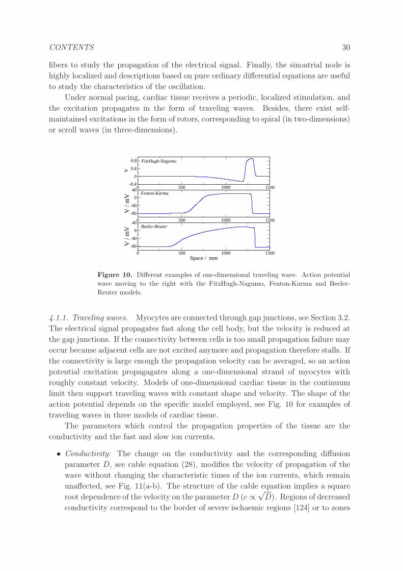
Under normal pacing, cardiac tissue receives a periodic, localized stimulation, and
the excitation propagates in the form of traveling waves. Besides, there exist self-
maintained excitations in the form of rotors, corresponding to spiral (in two-dimensions)
or scroll waves (in three-dimensions).
0 500 1000 1500-0,4
0
0,4
0,8
v
0 500 1000 1500
-80
-40
0
40
V /
mV
0 500 1000 1500Space / mm
-80
-40
0
40
V /
mV
FitzHugh-Nagumo
Fenton-Karma
Beeler-Reuter
Figure 10. Different examples of one-dimensional traveling wave. Action potential
wave moving to the right with the FitzHugh-Nagumo, Fenton-Karma and Beeler-
Reuter models.
4.1.1. Traveling waves. Myocytes are connected through gap junctions, see Section 3.2.
The electrical signal propagates fast along the cell body, but the velocity is reduced at
the gap junctions. If the connectivity between cells is too small propagation failure may
occur because adjacent cells are not excited anymore and propagation therefore stalls. If
the connectivity is large enough the propagation velocity can be averaged, so an action
potential excitation propagagates along a one-dimensional strand of myocytes with
roughly constant velocity. Models of one-dimensional cardiac tissue in the continuum
limit then support traveling waves with constant shape and velocity. The shape of the
action potential depends on the specific model employed, see Fig. 10 for examples of
traveling waves in three models of cardiac tissue.
The parameters which control the propagation properties of the tissue are the
conductivity and the fast and slow ion currents.
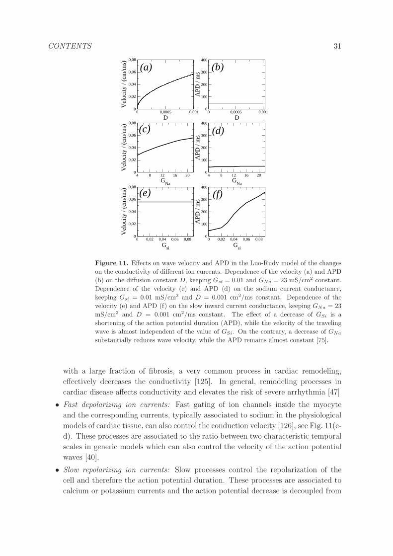
• Conductivity: The change on the conductivity and the corresponding diffusion
parameter D, see cable equation (28), modifies the velocity of propagation of the
wave without changing the characteristic times of the ion currents, which remain
unaffected, see Fig. 11(a-b). The structure of the cable equation implies a square
root dependence of the velocity on the parameterD (c ∝√D). Regions of decreased
conductivity correspond to the border of severe ischaemic regions [124] or to zones
CONTENTS 31
0 0,0005 0,001
D
0
0,02
0,04
0,06
0,08
Vel
ocity
/ (c
m/m
s)
0 0,0005 0,001
D
0
100
200
300
400
APD
/ m
s
0 0,02 0,04 0,06 0,08
Gsi
0
0,02
0,04
0,06
0,08
Vel
ocity
/ (c
m/m
s)
0 0,02 0,04 0,06 0,08
Gsi
0
100
200
300
400
APD
/ m
s
4 8 12 16 20
GNa
0
0,02
0,04
0,06
0,08V
eloc
ity /
(cm
/ms)
4 8 12 16 20
GNa
0
100
200
300
400
APD
/ m
s
(a) (b)
(c) (d)
(e) (f)
Figure 11. Effects on wave velocity and APD in the Luo-Rudy model of the changes
on the conductivity of different ion currents. Dependence of the velocity (a) and APD
(b) on the diffusion constant D, keeping Gsi = 0.01 and GNa = 23 mS/cm2 constant.
Dependence of the velocity (c) and APD (d) on the sodium current conductance,
keeping Gsi = 0.01 mS/cm2 and D = 0.001 cm2/ms constant. Dependence of the
velocity (e) and APD (f) on the slow inward current conductance, keeping GNa = 23
mS/cm2 and D = 0.001 cm2/ms constant. The effect of a decrease of GSi is a
shortening of the action potential duration (APD), while the velocity of the traveling
wave is almost independent of the value of GSi. On the contrary, a decrease of GNa
substantially reduces wave velocity, while the APD remains almost constant [75].
with a large fraction of fibrosis, a very common process in cardiac remodeling,
effectively decreases the conductivity [125]. In general, remodeling processes in
cardiac disease affects conductivity and elevates the risk of severe arrhythmia [47]
• Fast depolarizing ion currents: Fast gating of ion channels inside the myocyte
and the corresponding currents, typically associated to sodium in the physiological
models of cardiac tissue, can also control the conduction velocity [126], see Fig. 11(c-
d). These processes are associated to the ratio between two characteristic temporal
scales in generic models which can also control the velocity of the action potential
waves [40].
• Slow repolarizing ion currents: Slow processes control the repolarization of the
cell and therefore the action potential duration. These processes are associated to
calcium or potassium currents and the action potential decrease is decoupled from
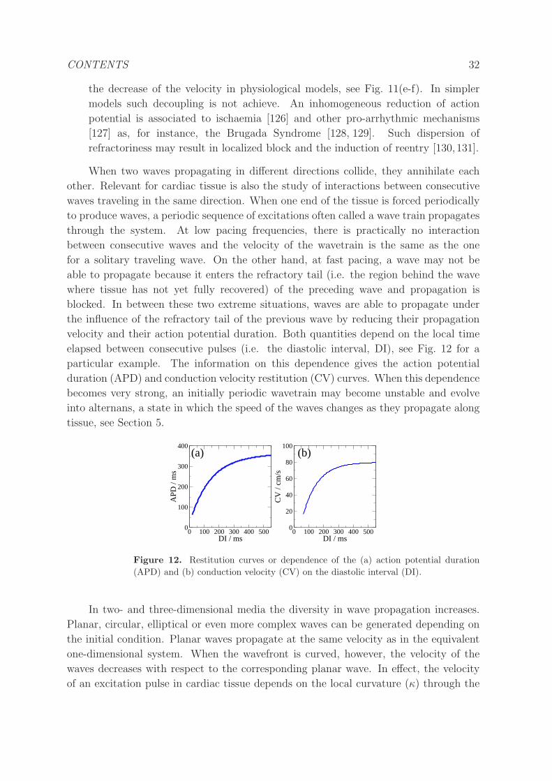
CONTENTS 32
the decrease of the velocity in physiological models, see Fig. 11(e-f). In simpler
models such decoupling is not achieve. An inhomogeneous reduction of action
potential is associated to ischaemia [126] and other pro-arrhythmic mechanisms
[127] as, for instance, the Brugada Syndrome [128, 129]. Such dispersion of
refractoriness may result in localized block and the induction of reentry [130,131].
When two waves propagating in different directions collide, they annihilate each
other. Relevant for cardiac tissue is also the study of interactions between consecutive
waves traveling in the same direction. When one end of the tissue is forced periodically
to produce waves, a periodic sequence of excitations often called a wave train propagates
through the system. At low pacing frequencies, there is practically no interaction
between consecutive waves and the velocity of the wavetrain is the same as the one
for a solitary traveling wave. On the other hand, at fast pacing, a wave may not be
able to propagate because it enters the refractory tail (i.e. the region behind the wave
where tissue has not yet fully recovered) of the preceding wave and propagation is
blocked. In between these two extreme situations, waves are able to propagate under
the influence of the refractory tail of the previous wave by reducing their propagation
velocity and their action potential duration. Both quantities depend on the local time
elapsed between consecutive pulses (i.e. the diastolic interval, DI), see Fig. 12 for a
particular example. The information on this dependence gives the action potential
duration (APD) and conduction velocity restitution (CV) curves. When this dependence
becomes very strong, an initially periodic wavetrain may become unstable and evolve
into alternans, a state in which the speed of the waves changes as they propagate along
tissue, see Section 5.
0 100 200 300 400 500DI / ms
0
100
200
300
400
APD
/ m
s
0 100 200 300 400 500DI / ms
0
20
40
60
80
100
CV
/ cm
/s
(a) (b)
Figure 12. Restitution curves or dependence of the (a) action potential duration
(APD) and (b) conduction velocity (CV) on the diastolic interval (DI).
In two- and three-dimensional media the diversity in wave propagation increases.
Planar, circular, elliptical or even more complex waves can be generated depending on
the initial condition. Planar waves propagate at the same velocity as in the equivalent
one-dimensional system. When the wavefront is curved, however, the velocity of the
waves decreases with respect to the corresponding planar wave. In effect, the velocity
of an excitation pulse in cardiac tissue depends on the local curvature (κ) through the
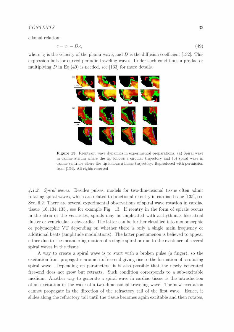
CONTENTS 33
eikonal relation:
c = c0 −Dκ, (49)
where c0 is the velocity of the planar wave, and D is the diffusion coefficient [132]. This
expression fails for curved periodic traveling waves. Under such conditions a pre-factor
multiplying D in Eq.(49) is needed, see [133] for more details.
Figure 13. Reentrant wave dynamics in experimental preparations. (a) Spiral wave
in canine atrium where the tip follows a circular trajectory and (b) spiral wave in
canine ventricle where the tip follows a linear trajectory. Reproduced with permission
from [134]. All rights reserved
4.1.2. Spiral waves. Besides pulses, models for two-dimensional tissue often admit
rotating spiral waves, which are related to functional re-entry in cardiac tissue [135], see
Sec. 6.2. There are several experimental observations of spiral wave rotation in cardiac
tissue [16, 134, 135], see for example Fig. 13. If reentry in the form of spirals occurs
in the atria or the ventricles, spirals may be implicated with arrhythmias like atrial
flutter or ventricular tachycardia. The latter can be further classified into monomorphic
or polymorphic VT depending on whether there is only a single main frequency or
additional beats (amplitude modulations). The latter phenomenon is believed to appear
either due to the meandering motion of a single spiral or due to the existence of several
spiral waves in the tissue.
A way to create a spiral wave is to start with a broken pulse (a finger), so the
excitation front propagates around its free-end giving rise to the formation of a rotating
spiral wave. Depending on parameters, it is also possible that the newly generated
free-end does not grow but retracts. Such condition corresponds to a sub-excitable
medium. Another way to generate a spiral wave in cardiac tissue is the introduction
of an excitation in the wake of a two-dimensional traveling wave. The new excitation
cannot propagate in the direction of the refractory tail of the first wave. Hence, it
slides along the refractory tail until the tissue becomes again excitable and then rotates,
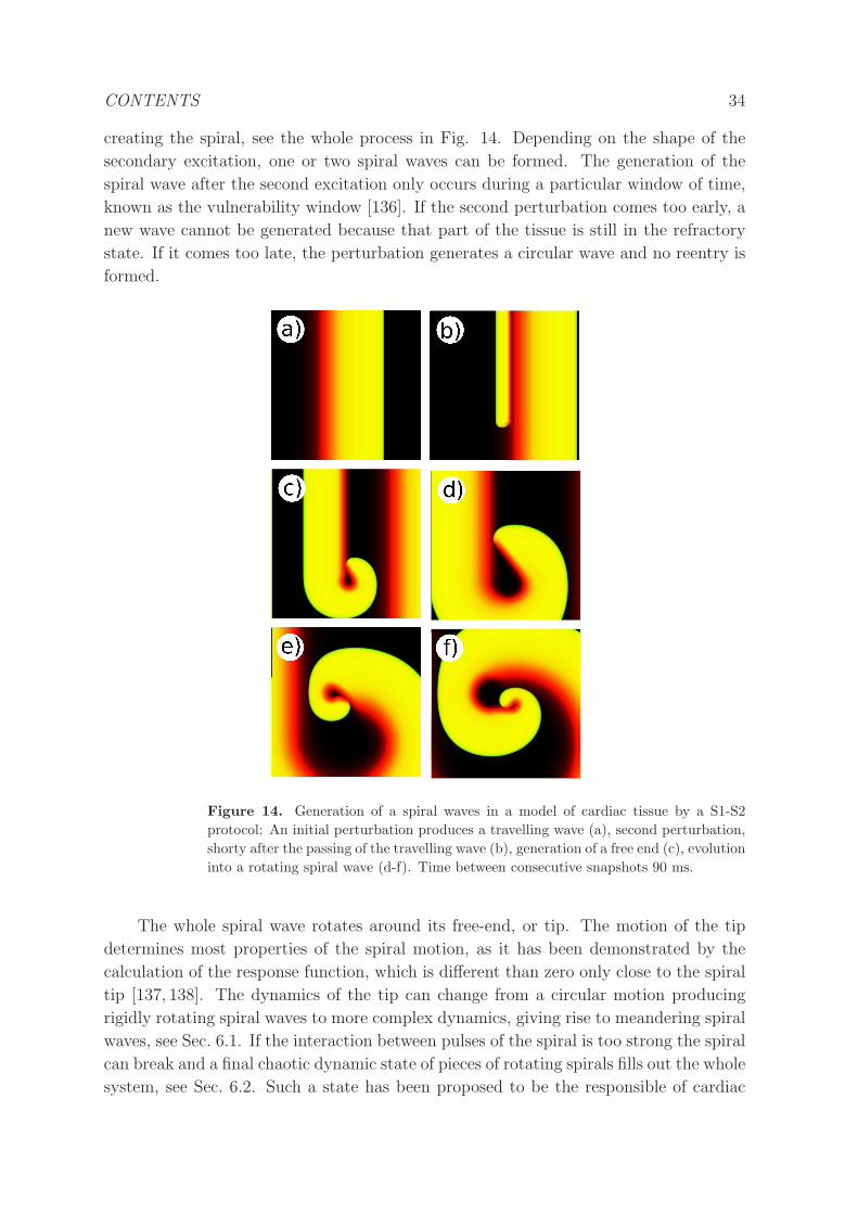
CONTENTS 34
creating the spiral, see the whole process in Fig. 14. Depending on the shape of the
secondary excitation, one or two spiral waves can be formed. The generation of the
spiral wave after the second excitation only occurs during a particular window of time,
known as the vulnerability window [136]. If the second perturbation comes too early, a
new wave cannot be generated because that part of the tissue is still in the refractory
state. If it comes too late, the perturbation generates a circular wave and no reentry is
formed.
Figure 14. Generation of a spiral waves in a model of cardiac tissue by a S1-S2
protocol: An initial perturbation produces a travelling wave (a), second perturbation,
shorty after the passing of the travelling wave (b), generation of a free end (c), evolution
into a rotating spiral wave (d-f). Time between consecutive snapshots 90 ms.
The whole spiral wave rotates around its free-end, or tip. The motion of the tip
determines most properties of the spiral motion, as it has been demonstrated by the
calculation of the response function, which is different than zero only close to the spiral
tip [137, 138]. The dynamics of the tip can change from a circular motion producing
rigidly rotating spiral waves to more complex dynamics, giving rise to meandering spiral
waves, see Sec. 6.1. If the interaction between pulses of the spiral is too strong the spiral
can break and a final chaotic dynamic state of pieces of rotating spirals fills out the whole
system, see Sec. 6.2. Such a state has been proposed to be the responsible of cardiac
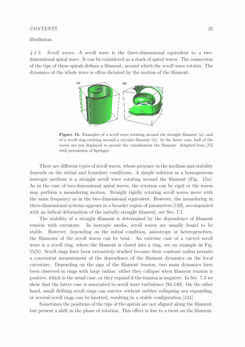
CONTENTS 35
fibrillation.
4.1.3. Scroll waves. A scroll wave is the three-dimensional equivalent to a two-
dimensional spiral wave. It can be considered as a stack of spiral waves. The connection
of the tips of these spirals defines a filament, around which the scroll wave rotates. The
dynamics of the whole wave is often dictated by the motion of the filament.
Figure 15. Examples of a scroll wave rotating around the straight filament (a), and
of a scroll ring rotating around a circular filament (b). In the latter case, half of the
waves are not displayed to permit the visualization the filament. Adapted from [75]
with permission of Springer.
There are different types of scroll waves, whose presence in the medium and stability
depends on the initial and boundary conditions. A simple solution in a homogeneous
isotropic medium is a straight scroll wave rotating around the filament (Fig. 15a).
As in the case of two-dimensional spiral waves, the rotation can be rigid or the waves
may perform a meandering motion. Straight rigidly rotating scroll waves move with
the same frequency as in the two-dimensional equivalent. However, the meandering in
three-dimensional systems appears in a broader region of parameters [139], accompanied
with an helical deformation of the initially straight filament, see Sec. 7.1.
The stability of a straight filament is determined by the dependence of filament
tension with curvature. In isotropic media, scroll waves are usually found to be
stable. However, depending on the initial condition, anisotropy or heterogeneities,
the filaments of the scroll waves can be bent. An extreme case of a curved scroll
wave is a scroll ring, where the filament is closed into a ring, see an example in Fig.
15(b). Scroll rings have been extensively studied because their constant radius permits
a convenient measurement of the dependence of the filament dynamics on the local
curvature. Depending on the sign of the filament tension, two main dynamics have
been observed in rings with large radius: either they collapse when filament tension is
positive, which is the usual case, or they expand if the tension is negative. In Sec. 7.3 we
show that the latter case is associated to scroll wave turbulence [93,140]. On the other
hand, small drifting scroll rings can survive without neither collapsing nor expanding,
or several scroll rings can be knotted, resulting in a stable configuration [141].
Sometimes the positions of the tips of the spirals are not aligned along the filament,
but present a shift in the phase of rotation. This effect is due to a twist on the filament.
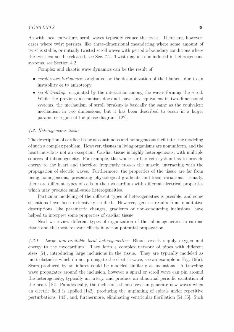
CONTENTS 36
As with local curvature, scroll waves typically reduce the twist. There are, however,
cases where twist persists, like three-dimensional meandering where some amount of
twist is stable, or initially twisted scroll waves with periodic boundary conditions where
the twist cannot be released, see Sec. 7.2. Twist may also be induced in heterogeneous
systems, see Section 4.2.
Complex and chaotic wave dynamics can be the result of:
• scroll wave turbulence: originated by the destabilization of the filament due to an
instability or to anisotropy.
• scroll breakup: originated by the interaction among the waves forming the scroll.
While the previous mechanism does not have any equivalent in two-dimensional
systems, the mechanism of scroll breakup is basically the same as the equivalent
mechanism in two dimensions, but it has been described to occur in a larger
parameter region of the phase diagram [122].
4.2. Heterogeneous tissue
The description of cardiac tissue as continuous and homogeneous facilitates the modeling
of such a complex problem. However, tissues in living organisms are nonuniform, and the
heart muscle is not an exception. Cardiac tissue is highly heterogeneous, with multiple
sources of inhomogeneity. For example, the whole cardiac vein system has to provide
energy to the heart and therefore frequently crosses the muscle, interacting with the
propagation of electric waves. Furthermore, the properties of the tissue are far from
being homogeneous, presenting physiological gradients and local variations. Finally,
there are different types of cells in the myocardium with different electrical properties
which may produce small-scale heterogeneities.
Particular modeling of the different types of heterogeneities is possible, and some
situations have been extensively studied. However, generic results from qualitative
descriptions, like parametric changes, gradients or non-conducting inclusions, have
helped to interpret some properties of cardiac tissue.
Next we review different types of organization of the inhomogeneities in cardiac
tissue and the most relevant effects in action potential propagation.
4.2.1. Large non-excitable local heterogeneities. Blood vessels supply oxygen and
energy to the myocardium. They form a complex network of pipes with different
sizes [54], introducing large inclusions in the tissue. They are typically modeled as
inert obstacles which do not propagate the electric wave, see an example in Fig. 16(a).
Scars produced by an infarct could be modeled similarly as inclusions. A traveling
wave propagates around the inclusion, however a spiral or scroll wave can pin around
the heterogeneity, typically an artery, and produce an abnormal periodic excitation of
the heart [16]. Paradoxically, the inclusions themselves can generate new waves when
an electric field is applied [142], producing the unpinning of spirals under repetitive
perturbations [143], and, furthermore, eliminating ventricular fibrillation [54, 55]. Such
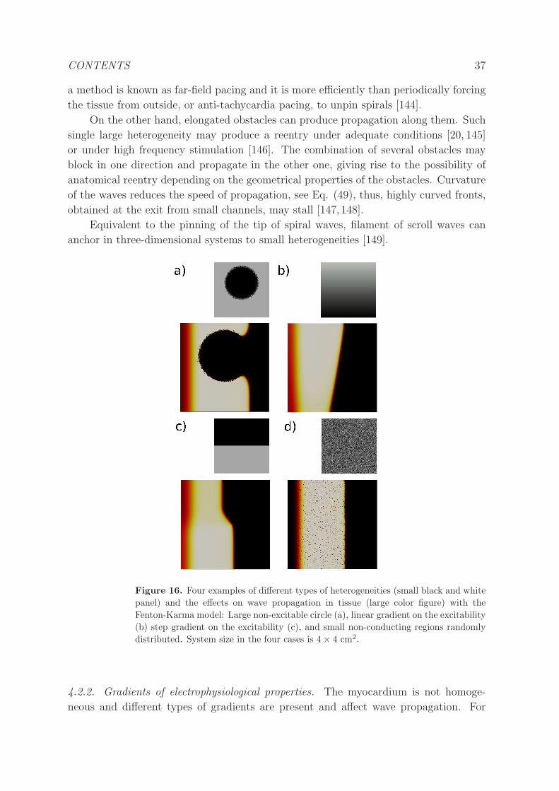
CONTENTS 37
a method is known as far-field pacing and it is more efficiently than periodically forcing
the tissue from outside, or anti-tachycardia pacing, to unpin spirals [144].
On the other hand, elongated obstacles can produce propagation along them. Such
single large heterogeneity may produce a reentry under adequate conditions [20, 145]
or under high frequency stimulation [146]. The combination of several obstacles may
block in one direction and propagate in the other one, giving rise to the possibility of
anatomical reentry depending on the geometrical properties of the obstacles. Curvature
of the waves reduces the speed of propagation, see Eq. (49), thus, highly curved fronts,
obtained at the exit from small channels, may stall [147,148].
Equivalent to the pinning of the tip of spiral waves, filament of scroll waves can
anchor in three-dimensional systems to small heterogeneities [149].
Figure 16. Four examples of different types of heterogeneities (small black and white
panel) and the effects on wave propagation in tissue (large color figure) with the
Fenton-Karma model: Large non-excitable circle (a), linear gradient on the excitability
(b) step gradient on the excitability (c), and small non-conducting regions randomly
distributed. System size in the four cases is 4× 4 cm2.
4.2.2. Gradients of electrophysiological properties. The myocardium is not homoge-
neous and different types of gradients are present and affect wave propagation. For
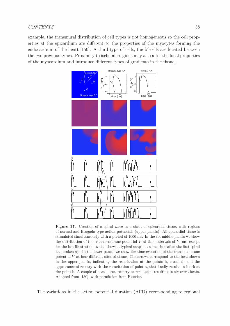
CONTENTS 38
example, the transmural distribution of cell types is not homogeneous so the cell prop-
erties at the epicardium are different to the properties of the myocytes forming the
endocardium of the heart [150]. A third type of cells, the M-cells are located between
the two previous types. Proximity to ischemic regions may also alter the local properties
of the myocardium and introduce different types of gradients in the tissue.
Brugada−type AP
c*
b*
normal AP
0 200time (ms)
-80
-40
0
Vm
(m
V)
Brugada-type AP
0 200time (ms)
-80
-40
0
Vm
(m
V)
Normal AP
d
a
b
c
a*d
*
Figure 17. Creation of a spiral wave in a sheet of epicardial tissue, with regions
of normal and Brugada-type action potentials (upper panels). All epicardial tissue is
stimulated simultaneously with a period of 1000 ms. In the six middle panels we show
the distribution of the transmembrane potential V at time intervals of 50 ms, except
for the last illustration, which shows a typical snapshot some time after the first spiral
has broken up. In the lower panels we show the time evolution of the transmembrane
potential V at four different sites of tissue. The arrows correspond to the beat shown
in the upper panels, indicating the reexcitation at the points b, c and d, and the
appearance of reentry with the reexcitation of point a, that finally results in block at
the point b. A couple of beats later, reentry occurs again, resulting in six extra beats.
Adapted from [130], with permission from Elsevier.
The variations in the action potential duration (APD) corresponding to regional
CONTENTS 39
differences of electrophysiological properties result in dispersion of repolarization. This
has been linked to an increased risk of cardiac death [151] and, in particular, to a higher
risk of arrhythmogenicity in short QT, long QT and Brugada syndromes [152–155]. In
Brugada syndrome, for instance, dispersion of repolarization is thought to be caused by
an abbreviation of the APD of the right ventricular epicardium due to loss of the action
potential dome [156]. Then, a region of depolarized tissue (during calcium current
entrance, or phase-2 of the AP) can re-excite adjacent regions that exhibit shorter
action potential duration (APD) [130], producing an extrasystole which can eventually
initate phase-2 reentry (see Figure 17). This same mechanism has also been proposed to
explain reentry associated to dispersion of repolarization around ischemic regions [157].
Thus, reexcitation due to phase-2 reentry needs two conditions to be met: first, that a
heterogeneous loss of dome is produced in tissue and, second, that the spike-and-dome
regions are able to reexcitate the loss-dome areas. The latter has been shown to occur
due to the propagation of a slow pulse sustained by the inward calcium current, that is
then able to reexcitate adjacent tissue [131].
Linear Gradients. A continuous change on the properties of propagation will cause an
acceleration (deceleration) of the pulse moving in the direction (opposite direction) of
the excitability gradient. It may also modify the vulnerability window and even induce
conduction block [136].
In a two-dimensional slab of tissue a gradient of excitability induces variations in
wave velocity, see Fig. 16(b), and produces the drift of a spiral wave pushed by the
change of the rotation frequency during each period of rotation due to the gradient.
The direction of the drift depends on the model parameters [158]. A gradient in the gap
junction conductances produces similar behavior [159].
A straight scroll wave with the filament parallel to a gradient of excitability produces
the formation of constant twist along the filament [160]. Furthermore, if the scroll wave
is not oriented in the direction of the gradient it turns and tries to align in the same
direction. On the other hand, scroll rings are also affected by gradients and the normal
vector of the filament plane also orientate with the gradient [161].
Step Gradients. Sudden changes on the excitability or in other properties of the
myocytes may substantially affect the dynamics of the waves. A traveling wave
propagating from a region of higher excitability to a region of lower excitability will
change velocity adapting to the local properties of the the tissue. However, in the
opposite direction it may block and do not propagate.
Step gradients produce two different velocities, see Fig. 16(c). Spiral waves located
at the border of two regions with different properties of propagation may be affected if
the core of the spiral rotates crossing this border. The difference of rotating frequencies
produces a directed drift along the boundary between the two regions [162].
A scroll wave oriented perpendicularly to the border between two regions with
different propagation properties will deform. The filament in the region with faster
CONTENTS 40
rotation frequency will maintain its original shape. In the other region, the filament
twists because of the difference in frequency. Thus, to keep the filament connected and
compensate this phase difference twist develops [160].
4.2.3. Localized heterogeneity. The accumulation of different types of cells or the
presence of light infarct areas or scars may result in a localized change in excitability
of a determinate region of the tissue. Apart from the effects of the borders discussed in
the previous section, the shape, size and degree of excitability of the heterogeneity may
be determinant for the propagation properties of the waves. A two-dimensional pulse
crossing a region with different excitability will change locally its velocity and curvature.
If the difference in excitability in this region in comparison with the rest of the medium
is large enough reentry can be produced [163].
One of the most accepted mechanism of reentry formation is the interaction of two
consecutive waves with a large heterogeneity formed by cells with a refractory period
larger than the rest [163–167]. The second pulse stops in the heterogeneity because of
the refractory state produced by the previous wave. It can, however, propagate outside
of the heterogeneity producing a free end which re-enters into the heterogeneity when
the refractory period ends.
4.2.4. Small-scale heterogeneities. Small-scale heterogeneities are inevitable and
omnipresent in cardiac tissues. This is due to the variability of individual cells,
the presence of different cell types as well as the potential inclusion of fibrotic cells
inside otherwise healthy tissue. Another factor is the discrete nature of the tissue
that is composed of myocytes separated by extracellular space filled with interstitial
fluids. As discussed in Section 3.2, homogenization procedures [8] are employed to
derive the bidomain equations of cardiac dynamics based on periodic arrangements of
cells and related periodic variation of medium properties [9, 10]. Often, the bidomain
equations are further reduced to the monodomain equations [11], resulting in a set of
coupled nonlinear reaction-diffusion equations that is the main model type discussed
in this review. A homogenization of reaction-diffusion equations with small-scale
heterogeneities was carried out recently [168, 169] to obtain effective diffusivities resp.
conductivities and effective local excitation kinetics assuming a random structure.
The procedure was validated with simulations in discrete models with randomly
assigned coupling between cells and/or local kinetics with small fraction of non-excitable
elements and/or blocked connections. Homogenization fails badly if such obstacles to
perturbation reach fractions close to percolation. Then, large cluster occur and the
assumption of homogenization regarding a large differences in scales between variation
of local kinetics and spatial coupling on the one hand and the typical interface width of
excitation on the other hand breaks down [168]. As a result, heterogeneities may induce
disruption and subsequent reentry, as has been observed in very schematic models [170],
in simplified ionic models [171], and in more complex models [172]. Homogenization
has also been used to predict effective wave speeds in periodic media [42, 173]. As long
CONTENTS 41
as the excitation front width is larger than the characteristic size of the heterogeneities
the wave speed is approximately constant. Interestingly, intermediate periods of the
heterogeneity length scale may yield conduction block of waves, whereas propagation is
possible at small and large length scales [173].
In contrast to such approximations of spatial homogeneity and/or smooth changes
of parameters in cardiac modeling, cardiac tissue may be modeled not as a continuous
medium but as a discrete interconnected collection of cells, some of which, e. g. the
fibroblasts, are non-excitable, see and example in Fig. 16(d).
Approximately two thirds of the volume of cardiac tissue is formed by myocytes,
the rest of the volume is basically composed by fibroblasts. Since the size of myocytes is
around five times larger than the size of the fibroblasts, the fibroblasts are the largest cell
population by number [174]. One of the main function of fibroblasts is the production
of the proteins forming the extracellular matrix (ECM) which give support to the whole
tissue. An excess production of such proteins leads to fibrosis, which increases the risk
of malfunction in the heart. It has been shown in in vitro experiments that fibroblasts
form gap junctions with myocytes [175] and, therefore, may be electrically active in the
tissue.
The effects of a large fraction of fibroblast in the myocardium and its implications
in the formation of arrhythmias have been recently studied [176]. Although commonly a
heterogeneous description of the tissue was considered in such studies, homogenization
techniques were also employed to create a tridomain model [177], which is an extension
of the bidomain model with an additional third phase representing the fibroblasts.
Nevertheless, fibroblasts are usually included in the modeling of tissue as non-excitable
elements in a discrete version of the cable equation. Because of the smaller size of the
fibroblasts with respect to the myocytes, they are sometimes included in the discrete
lattice as an additional connection to each myocyte [178, 179], or with a smaller size in
models at the sub-cellular scale [180,181].
The effect of fibrosis, details of tissue structure obtained from histology and
other heterogeneities on the cellular level have also been included in a number of
discrete models for cardiac tissue in two and three dimensions [171, 172, 182–189]. The
disconnection among myocytes has been also employed as a model to explain reentry
around the pulmonary vein in the atria [190], which is one of the major causes of atrial
fibrillation [191], and in the formation of ectopic pacemakers [171].
In general the inclusion of randomly distributed non-excitable cells or the
uncoupling of myocites produces a reduction of wave velocity and an increase of spiral
period [192, 193]. It can stabilize spiral waves and preclude their breakup, typically
occurring at rapid rotation frequencies [194]. In all the different models that incorporate
non-excitable tissue, a decrease in the velocity of wave propagation is observed, that
can induce the formation of reentries [171, 190, 194] due to the source-sink mismatch
mechanism [25,195], see a realization of such reentry formation in Fig. 18.
On the other hand, a heterogeneous description of the medium is also particularly
convenient for the modeling of cell cultures. In this case cells grow in vitro, establishing
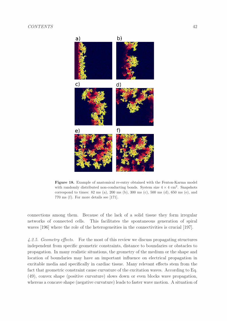
CONTENTS 42
Figure 18. Example of anatomical re-entry obtained with the Fenton-Karma model
with randomly distributed non-conducting bonds. System size 4 × 4 cm2. Snapshots
correspond to times: 82 ms (a), 200 ms (b), 300 ms (c), 500 ms (d), 650 ms (e), and
770 ms (f). For more details see [171].
connections among them. Because of the lack of a solid tissue they form irregular
networks of connected cells. This facilitates the spontaneous generation of spiral
waves [196] where the role of the heterogeneities in the connectivities is crucial [197].
4.2.5. Geometry effects. For the most of this review we discuss propagating structures
independent from specific geometric constraints, distance to boundaries or obstacles to
propagation. In many realistic situations, the geometry of the medium or the shape and
location of boundaries may have an important influence on electrical propagation in
excitable media and specifically in cardiac tissue. Many relevant effects stem from the
fact that geometric constraint cause curvature of the excitation waves. According to Eq.
(49), convex shape (positive curvature) slows down or even blocks wave propagation,
whereas a concave shape (negative curvature) leads to faster wave motion. A situation of
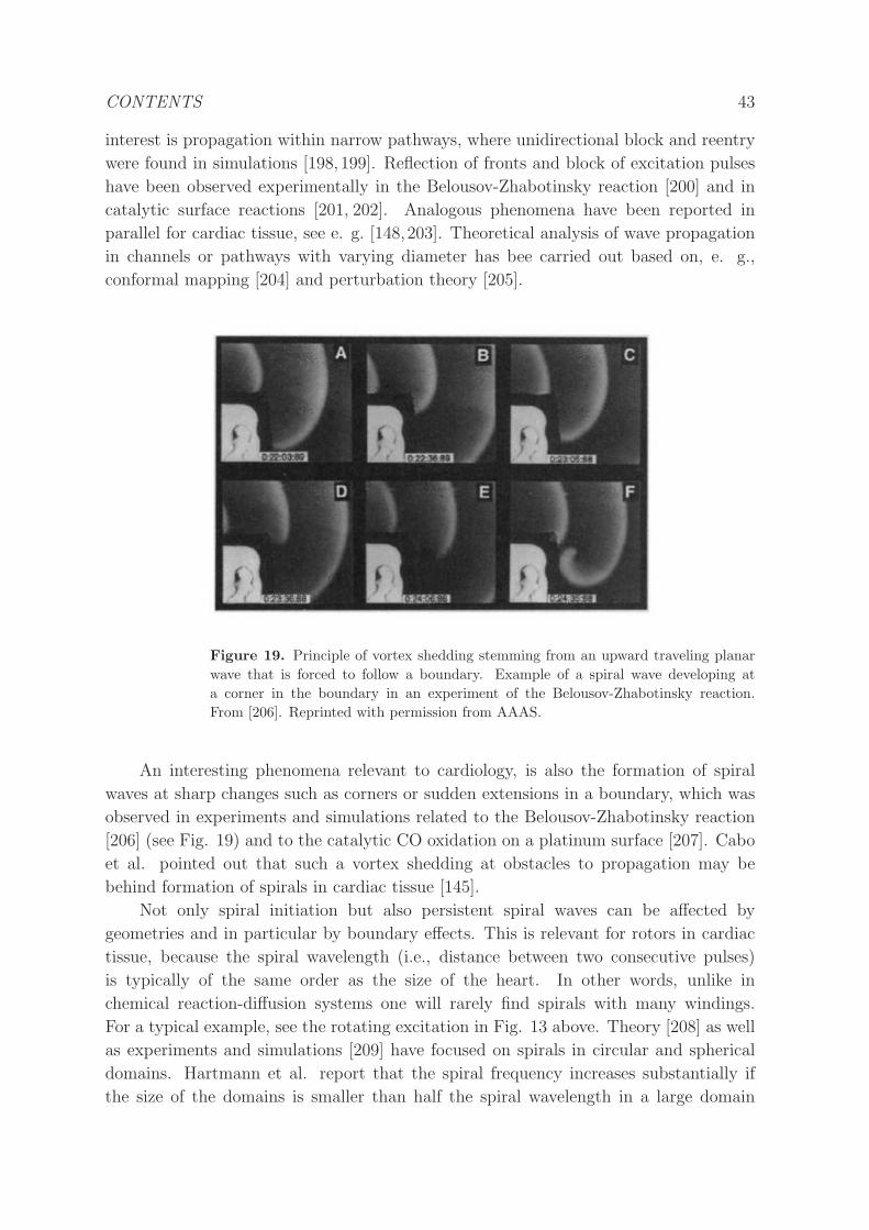
CONTENTS 43
interest is propagation within narrow pathways, where unidirectional block and reentry
were found in simulations [198, 199]. Reflection of fronts and block of excitation pulses
have been observed experimentally in the Belousov-Zhabotinsky reaction [200] and in
catalytic surface reactions [201, 202]. Analogous phenomena have been reported in
parallel for cardiac tissue, see e. g. [148,203]. Theoretical analysis of wave propagation
in channels or pathways with varying diameter has bee carried out based on, e. g.,
conformal mapping [204] and perturbation theory [205].
Figure 19. Principle of vortex shedding stemming from an upward traveling planar
wave that is forced to follow a boundary. Example of a spiral wave developing at
a corner in the boundary in an experiment of the Belousov-Zhabotinsky reaction.
From [206]. Reprinted with permission from AAAS.
An interesting phenomena relevant to cardiology, is also the formation of spiral
waves at sharp changes such as corners or sudden extensions in a boundary, which was
observed in experiments and simulations related to the Belousov-Zhabotinsky reaction
[206] (see Fig. 19) and to the catalytic CO oxidation on a platinum surface [207]. Cabo
et al. pointed out that such a vortex shedding at obstacles to propagation may be
behind formation of spirals in cardiac tissue [145].
Not only spiral initiation but also persistent spiral waves can be affected by
geometries and in particular by boundary effects. This is relevant for rotors in cardiac
tissue, because the spiral wavelength (i.e., distance between two consecutive pulses)
is typically of the same order as the size of the heart. In other words, unlike in
chemical reaction-diffusion systems one will rarely find spirals with many windings.
For a typical example, see the rotating excitation in Fig. 13 above. Theory [208] as well
as experiments and simulations [209] have focused on spirals in circular and spherical
domains. Hartmann et al. report that the spiral frequency increases substantially if
the size of the domains is smaller than half the spiral wavelength in a large domain
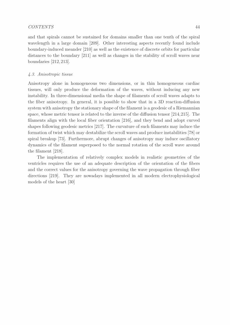
CONTENTS 44
and that spirals cannot be sustained for domains smaller than one tenth of the spiral
wavelength in a large domain [209]. Other interesting aspects recently found include
boundary-induced meander [210] as well as the existence of discrete orbits for particular
distances to the boundary [211] as well as changes in the stability of scroll waves near
boundaries [212,213].
4.3. Anisotropic tissue
Anisotropy alone in homogeneous two dimensions, or in thin homogeneous cardiac
tissues, will only produce the deformation of the waves, without inducing any new
instability. In three-dimensional media the shape of filaments of scroll waves adapts to
the fiber anisotropy. In general, it is possible to show that in a 3D reaction-diffusion
system with anisotropy the stationary shape of the filament is a geodesic of a Riemannian
space, whose metric tensor is related to the inverse of the diffusion tensor [214,215]. The
filaments align with the local fiber orientation [216], and they bend and adopt curved
shapes following geodesic metrics [217]. The curvature of such filaments may induce the
formation of twist which may destabilize the scroll waves and produce instabilities [78] or
spiral breakup [73]. Furthermore, abrupt changes of anisotropy may induce oscillatory
dynamics of the filament superposed to the normal rotation of the scroll wave around
the filament [218].
The implementation of relatively complex models in realistic geometries of the
ventricles requires the use of an adequate description of the orientation of the fibers
and the correct values for the anisotropy governing the wave propagation through fiber
directions [219]. They are nowadays implemented in all modern electrophysiological
models of the heart [30]
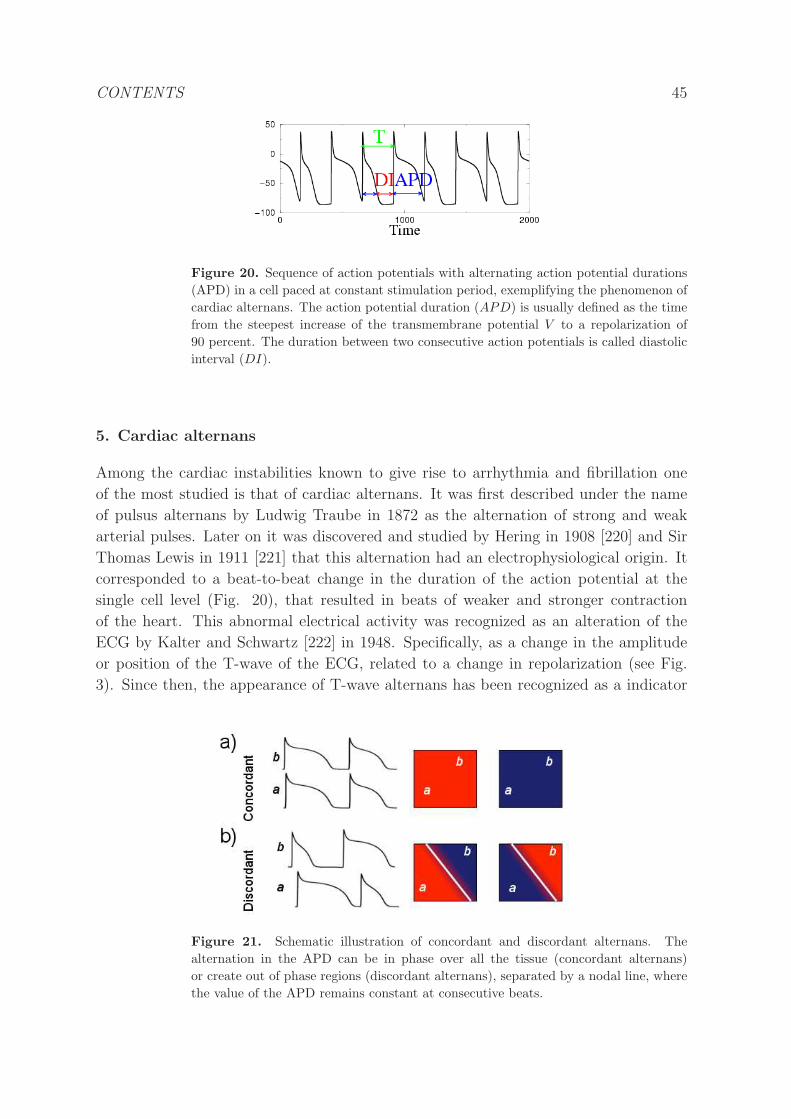
CONTENTS 45
Figure 20. Sequence of action potentials with alternating action potential durations
(APD) in a cell paced at constant stimulation period, exemplifying the phenomenon of
cardiac alternans. The action potential duration (APD) is usually defined as the time
from the steepest increase of the transmembrane potential V to a repolarization of
90 percent. The duration between two consecutive action potentials is called diastolic
interval (DI).
5. Cardiac alternans
Among the cardiac instabilities known to give rise to arrhythmia and fibrillation one
of the most studied is that of cardiac alternans. It was first described under the name
of pulsus alternans by Ludwig Traube in 1872 as the alternation of strong and weak
arterial pulses. Later on it was discovered and studied by Hering in 1908 [220] and Sir
Thomas Lewis in 1911 [221] that this alternation had an electrophysiological origin. It
corresponded to a beat-to-beat change in the duration of the action potential at the
single cell level (Fig. 20), that resulted in beats of weaker and stronger contraction
of the heart. This abnormal electrical activity was recognized as an alteration of the
ECG by Kalter and Schwartz [222] in 1948. Specifically, as a change in the amplitude
or position of the T-wave of the ECG, related to a change in repolarization (see Fig.
3). Since then, the appearance of T-wave alternans has been recognized as a indicator
Figure 21. Schematic illustration of concordant and discordant alternans. The
alternation in the APD can be in phase over all the tissue (concordant alternans)
or create out of phase regions (discordant alternans), separated by a nodal line, where
the value of the APD remains constant at consecutive beats.
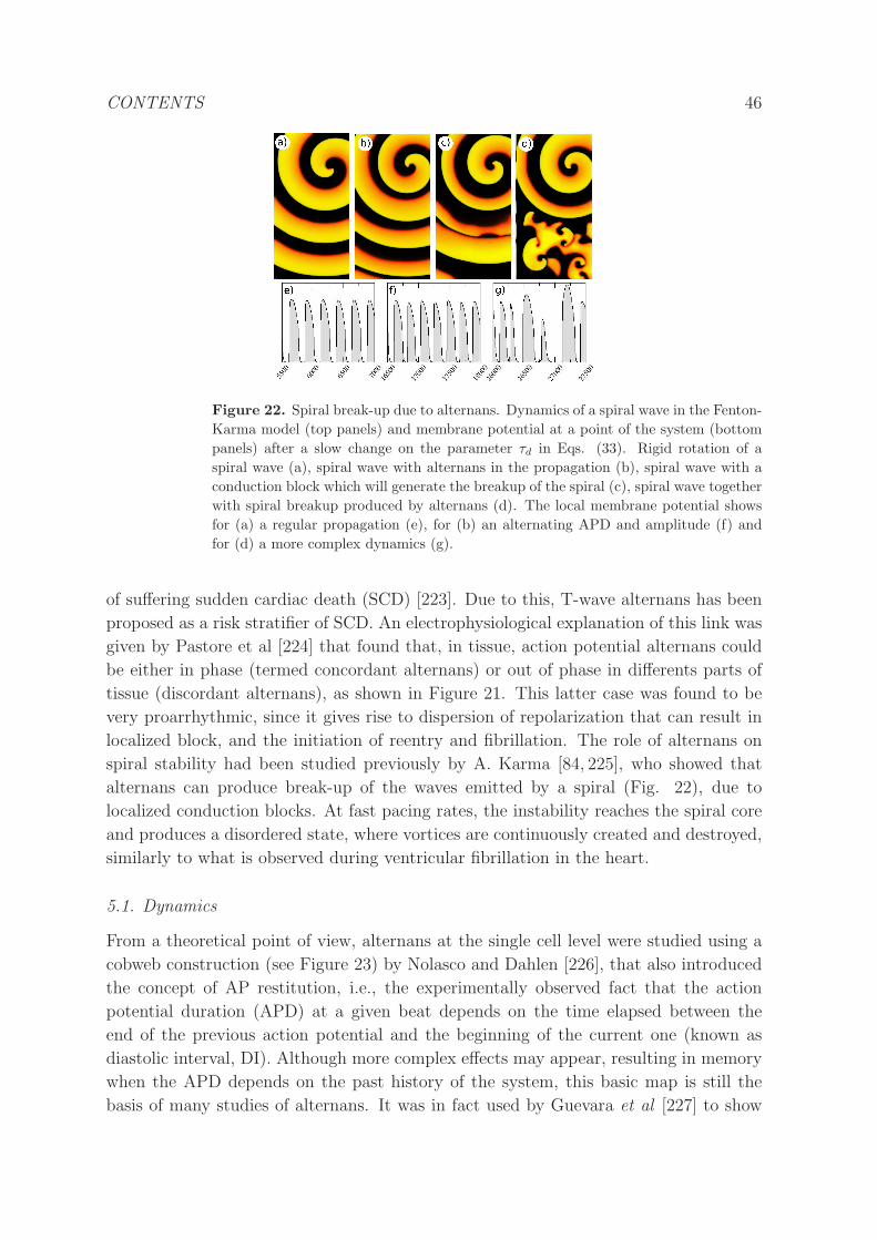
CONTENTS 46
Figure 22. Spiral break-up due to alternans. Dynamics of a spiral wave in the Fenton-
Karma model (top panels) and membrane potential at a point of the system (bottom
panels) after a slow change on the parameter τd in Eqs. (33). Rigid rotation of a
spiral wave (a), spiral wave with alternans in the propagation (b), spiral wave with a
conduction block which will generate the breakup of the spiral (c), spiral wave together
with spiral breakup produced by alternans (d). The local membrane potential shows
for (a) a regular propagation (e), for (b) an alternating APD and amplitude (f) and
for (d) a more complex dynamics (g).
of suffering sudden cardiac death (SCD) [223]. Due to this, T-wave alternans has been
proposed as a risk stratifier of SCD. An electrophysiological explanation of this link was
given by Pastore et al [224] that found that, in tissue, action potential alternans could
be either in phase (termed concordant alternans) or out of phase in differents parts of
tissue (discordant alternans), as shown in Figure 21. This latter case was found to be
very proarrhythmic, since it gives rise to dispersion of repolarization that can result in
localized block, and the initiation of reentry and fibrillation. The role of alternans on
spiral stability had been studied previously by A. Karma [84, 225], who showed that
alternans can produce break-up of the waves emitted by a spiral (Fig. 22), due to
localized conduction blocks. At fast pacing rates, the instability reaches the spiral core
and produces a disordered state, where vortices are continuously created and destroyed,
similarly to what is observed during ventricular fibrillation in the heart.
5.1. Dynamics
From a theoretical point of view, alternans at the single cell level were studied using a
cobweb construction (see Figure 23) by Nolasco and Dahlen [226], that also introduced
the concept of AP restitution, i.e., the experimentally observed fact that the action
potential duration (APD) at a given beat depends on the time elapsed between the
end of the previous action potential and the beginning of the current one (known as
diastolic interval, DI). Although more complex effects may appear, resulting in memory
when the APD depends on the past history of the system, this basic map is still the
basis of many studies of alternans. It was in fact used by Guevara et al [227] to show
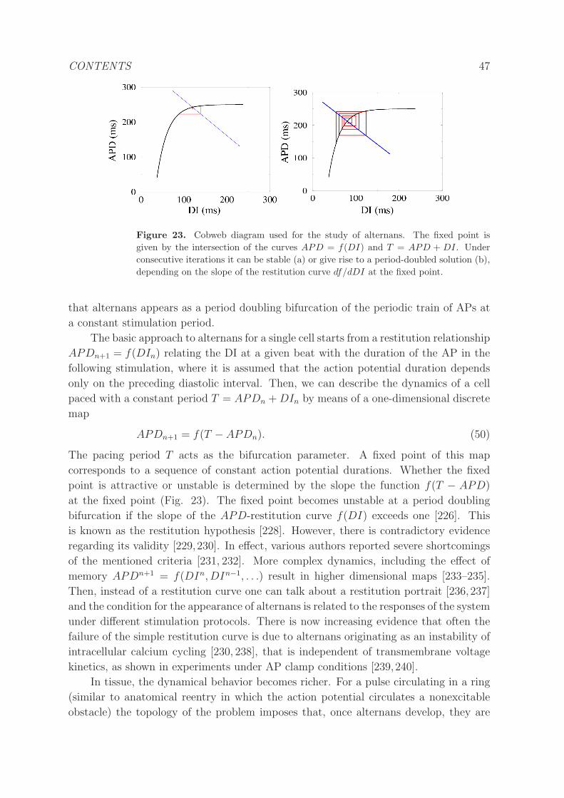
CONTENTS 47
Figure 23. Cobweb diagram used for the study of alternans. The fixed point is
given by the intersection of the curves APD = f(DI) and T = APD + DI. Under
consecutive iterations it can be stable (a) or give rise to a period-doubled solution (b),
depending on the slope of the restitution curve df/dDI at the fixed point.
that alternans appears as a period doubling bifurcation of the periodic train of APs at
a constant stimulation period.
The basic approach to alternans for a single cell starts from a restitution relationship
APDn+1 = f(DIn) relating the DI at a given beat with the duration of the AP in the
following stimulation, where it is assumed that the action potential duration depends
only on the preceding diastolic interval. Then, we can describe the dynamics of a cell
paced with a constant period T = APDn +DIn by means of a one-dimensional discrete
map
APDn+1 = f(T − APDn). (50)
The pacing period T acts as the bifurcation parameter. A fixed point of this map
corresponds to a sequence of constant action potential durations. Whether the fixed
point is attractive or unstable is determined by the slope the function f(T − APD)
at the fixed point (Fig. 23). The fixed point becomes unstable at a period doubling
bifurcation if the slope of the APD-restitution curve f(DI) exceeds one [226]. This
is known as the restitution hypothesis [228]. However, there is contradictory evidence
regarding its validity [229,230]. In effect, various authors reported severe shortcomings
of the mentioned criteria [231, 232]. More complex dynamics, including the effect of
memory APDn+1 = f(DIn, DIn−1, . . .) result in higher dimensional maps [233–235].
Then, instead of a restitution curve one can talk about a restitution portrait [236, 237]
and the condition for the appearance of alternans is related to the responses of the system
under different stimulation protocols. There is now increasing evidence that often the
failure of the simple restitution curve is due to alternans originating as an instability of
intracellular calcium cycling [230, 238], that is independent of transmembrane voltage
kinetics, as shown in experiments under AP clamp conditions [239,240].
In tissue, the dynamical behavior becomes richer. For a pulse circulating in a ring
(similar to anatomical reentry in which the action potential circulates a nonexcitable
obstacle) the topology of the problem imposes that, once alternans develop, they are
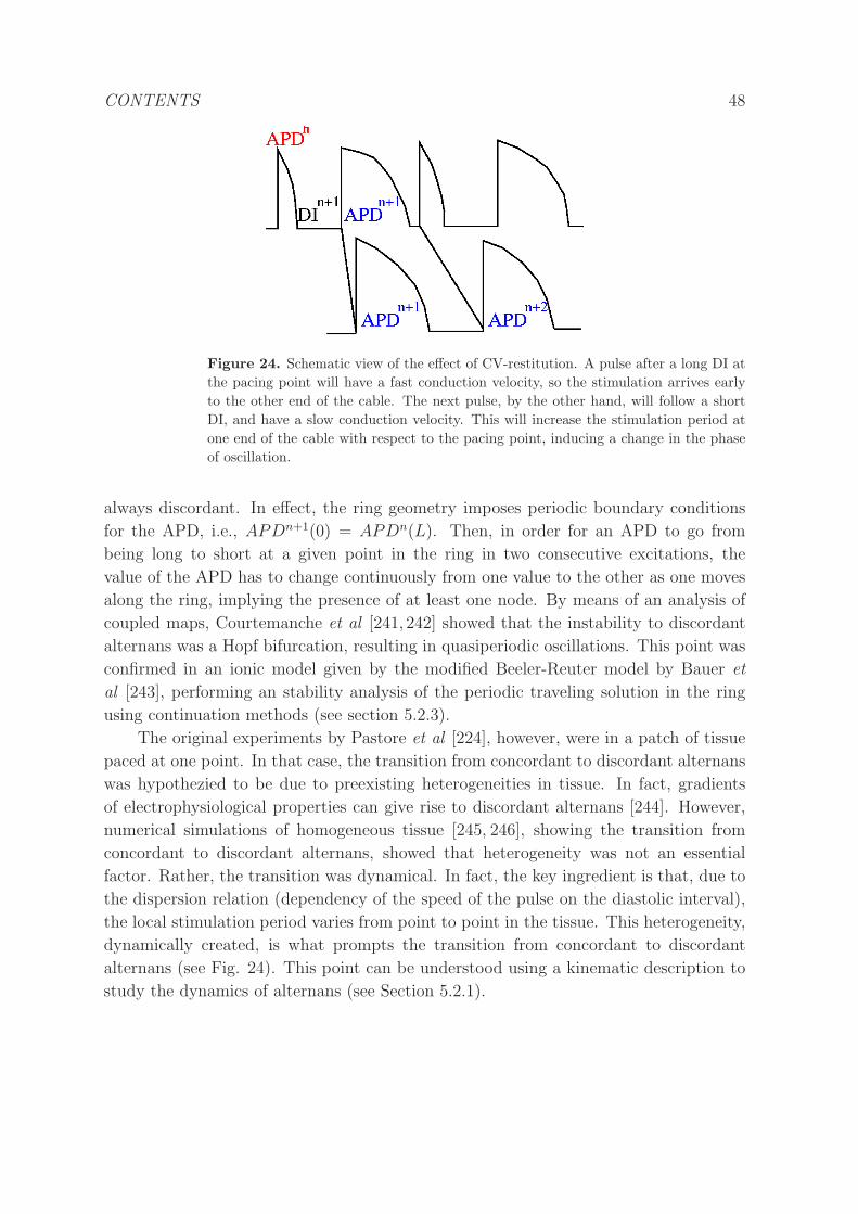
CONTENTS 48
Figure 24. Schematic view of the effect of CV-restitution. A pulse after a long DI at
the pacing point will have a fast conduction velocity, so the stimulation arrives early
to the other end of the cable. The next pulse, by the other hand, will follow a short
DI, and have a slow conduction velocity. This will increase the stimulation period at
one end of the cable with respect to the pacing point, inducing a change in the phase
of oscillation.
always discordant. In effect, the ring geometry imposes periodic boundary conditions
for the APD, i.e., APDn+1(0) = APDn(L). Then, in order for an APD to go from
being long to short at a given point in the ring in two consecutive excitations, the
value of the APD has to change continuously from one value to the other as one moves
along the ring, implying the presence of at least one node. By means of an analysis of
coupled maps, Courtemanche et al [241, 242] showed that the instability to discordant
alternans was a Hopf bifurcation, resulting in quasiperiodic oscillations. This point was
confirmed in an ionic model given by the modified Beeler-Reuter model by Bauer et
al [243], performing an stability analysis of the periodic traveling solution in the ring
using continuation methods (see section 5.2.3).
The original experiments by Pastore et al [224], however, were in a patch of tissue
paced at one point. In that case, the transition from concordant to discordant alternans
was hypothezied to be due to preexisting heterogeneities in tissue. In fact, gradients
of electrophysiological properties can give rise to discordant alternans [244]. However,
numerical simulations of homogeneous tissue [245, 246], showing the transition from
concordant to discordant alternans, showed that heterogeneity was not an essential
factor. Rather, the transition was dynamical. In fact, the key ingredient is that, due to
the dispersion relation (dependency of the speed of the pulse on the diastolic interval),
the local stimulation period varies from point to point in the tissue. This heterogeneity,
dynamically created, is what prompts the transition from concordant to discordant
alternans (see Fig. 24). This point can be understood using a kinematic description to
study the dynamics of alternans (see Section 5.2.1).
CONTENTS 49
5.2. Theory and Methods
Alternans in a one-dimensional geometry, either with periodic boundary conditions (a
pulse circulating in a ring), or in a paced cable, can be studied using a kinematic
description that provides the local values of the pacing period and APD in terms of the
restitution properties of the tissue. This provides a description of the system that is
valid even in the nonlinear regime, so it can be used to study, for instance, conduction
blocks. Close to the onset of alternans it is possible to derive amplitude equations for
the spatio-temporal dynamics of alternans. Even if these equations can be derived from
the kinematic equations, they can also be written down based on general symmetry
properties of the bifurcation to alternans and, therefore, reproduce generic properties
of the dynamics. Besides, one can analyze the bifurcation to alternans through a full
linear stability analysis of the cable equations. For this one can exploit the symmetry
properties of a pulse circulating in a ring. A full linear stability analysis for the paced
case is, at this moment, missing.
5.2.1. Kinematic description of alternans. Let us consider the case of a cable paced at
one end x = 0 with period T0. Then, we characterize the time at which the wavefront
and the waveback pass through a given point of tissue x by:
tf (x) = tf (0) +
∫ x
0
dx′
c(x′), (51)
tb(x) = tf (x) + APD(x); (52)
where c(x) is the velocity of the wavefront at position x. Knowing c(x) and APD(x) at
every point in space, then the system is completely determined. From the restitution
curves, we know that these variables will depend on position through the value of the
diastolic interval DI at that point, so c(x) = CV [DI(x)], APD(x) = f [DI(x)]. Besides,
at each point we have that local period of stimulation corresponding to the beat n is
T n(x) = APDn(x) +DIn(x), so
DIn(x) = T n(x)− f [DIn−1(x)], (53)
but
T n+1(x) = tn+1f (x)−tnf (x) = T0+
∫ x
0
dx′
CV [DIn+1(x′)]−∫ x
0
dx′
CV [DIn(x′)];(54)
where T0 = tn+1f (0)− tnf (0) is the pacing period at the origin.
Eqs. (53)-(54) constitute a closed set of discrete time equations (maps) that can
be used to study the stability of a pulse in tissue. However, there is a missing point
that happens to be crucial, this is, that the restitution curve of a given cell in tissue is
actually affected by electrotonic current coming from neighboring cells. During pulse
propagation, the electrotonic current coming from the left and right neighboring cells
is different, meaning that the change in the restitution curve must break the left-right
symmetry. The easiest way to include this effect is to consider diffusion plus a first
derivative, that breaks this symmetry (for a more rigorous derivation, see [247]). Then
ftissue(DIn) = fcell(DIn)− w∂xDIn + ξ2∂2xDIn. (55)
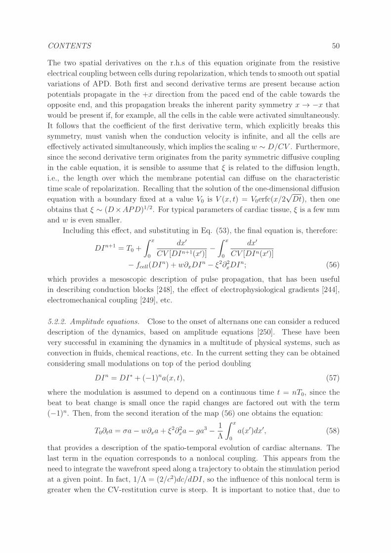
CONTENTS 50
The two spatial derivatives on the r.h.s of this equation originate from the resistive
electrical coupling between cells during repolarization, which tends to smooth out spatial
variations of APD. Both first and second derivative terms are present because action
potentials propagate in the +x direction from the paced end of the cable towards the
opposite end, and this propagation breaks the inherent parity symmetry x → −x that
would be present if, for example, all the cells in the cable were activated simultaneously.
It follows that the coefficient of the first derivative term, which explicitly breaks this
symmetry, must vanish when the conduction velocity is infinite, and all the cells are
effectively activated simultaneously, which implies the scaling w ∼ D/CV . Furthermore,
since the second derivative term originates from the parity symmetric diffusive coupling
in the cable equation, it is sensible to assume that ξ is related to the diffusion length,
i.e., the length over which the membrane potential can diffuse on the characteristic
time scale of repolarization. Recalling that the solution of the one-dimensional diffusion
equation with a boundary fixed at a value V0 is V (x, t) = V0erfc(x/2√Dt), then one
obtains that ξ ∼ (D×APD)1/2. For typical parameters of cardiac tissue, ξ is a few mm
and w is even smaller.
Including this effect, and substituting in Eq. (53), the final equation is, therefore:
DIn+1 = T0 +
∫ x
0
dx′
CV [DIn+1(x′)]−∫ x
0
dx′
CV [DIn(x′)]
− fcell(DIn) + w∂xDIn − ξ2∂2xDIn; (56)
which provides a mesoscopic description of pulse propagation, that has been useful
in describing conduction blocks [248], the effect of electrophysiological gradients [244],
electromechanical coupling [249], etc.
5.2.2. Amplitude equations. Close to the onset of alternans one can consider a reduced
description of the dynamics, based on amplitude equations [250]. These have been
very successful in examining the dynamics in a multitude of physical systems, such as
convection in fluids, chemical reactions, etc. In the current setting they can be obtained
considering small modulations on top of the period doubling
DIn = DI∗ + (−1)na(x, t), (57)
where the modulation is assumed to depend on a continuous time t = nT0, since the
beat to beat change is small once the rapid changes are factored out with the term
(−1)n. Then, from the second iteration of the map (56) one obtains the equation:
T0∂ta = σa− w∂xa+ ξ2∂2xa− ga3 − 1
Λ
∫ x
0
a(x′)dx′, (58)
that provides a description of the spatio-temporal evolution of cardiac alternans. The
last term in the equation corresponds to a nonlocal coupling. This appears from the
need to integrate the wavefront speed along a trajectory to obtain the stimulation period
at a given point. In fact, 1/Λ = (2/c2)dc/dDI, so the influence of this nonlocal term is
greater when the CV-restitution curve is steep. It is important to notice that, due to
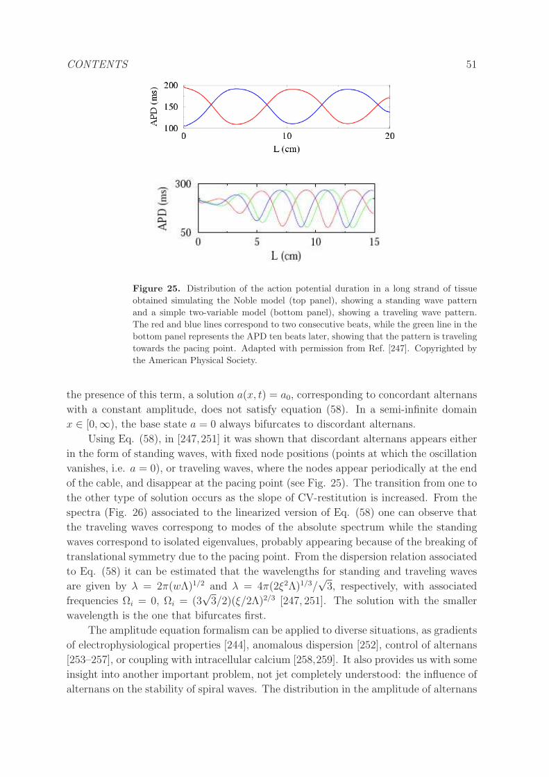
CONTENTS 51
Figure 25. Distribution of the action potential duration in a long strand of tissue
obtained simulating the Noble model (top panel), showing a standing wave pattern
and a simple two-variable model (bottom panel), showing a traveling wave pattern.
The red and blue lines correspond to two consecutive beats, while the green line in the
bottom panel represents the APD ten beats later, showing that the pattern is traveling
towards the pacing point. Adapted with permission from Ref. [247]. Copyrighted by
the American Physical Society.
the presence of this term, a solution a(x, t) = a0, corresponding to concordant alternans
with a constant amplitude, does not satisfy equation (58). In a semi-infinite domain
x ∈ [0,∞), the base state a = 0 always bifurcates to discordant alternans.
Using Eq. (58), in [247,251] it was shown that discordant alternans appears either
in the form of standing waves, with fixed node positions (points at which the oscillation
vanishes, i.e. a = 0), or traveling waves, where the nodes appear periodically at the end
of the cable, and disappear at the pacing point (see Fig. 25). The transition from one to
the other type of solution occurs as the slope of CV-restitution is increased. From the
spectra (Fig. 26) associated to the linearized version of Eq. (58) one can observe that
the traveling waves correspong to modes of the absolute spectrum while the standing
waves correspond to isolated eigenvalues, probably appearing because of the breaking of
translational symmetry due to the pacing point. From the dispersion relation associated
to Eq. (58) it can be estimated that the wavelengths for standing and traveling waves
are given by λ = 2π(wΛ)1/2 and λ = 4π(2ξ2Λ)1/3/√3, respectively, with associated
frequencies Ωi = 0, Ωi = (3√3/2)(ξ/2Λ)2/3 [247, 251]. The solution with the smaller
wavelength is the one that bifurcates first.
The amplitude equation formalism can be applied to diverse situations, as gradients
of electrophysiological properties [244], anomalous dispersion [252], control of alternans
[253–257], or coupling with intracellular calcium [258,259]. It also provides us with some
insight into another important problem, not jet completely understood: the influence of
alternans on the stability of spiral waves. The distribution in the amplitude of alternans
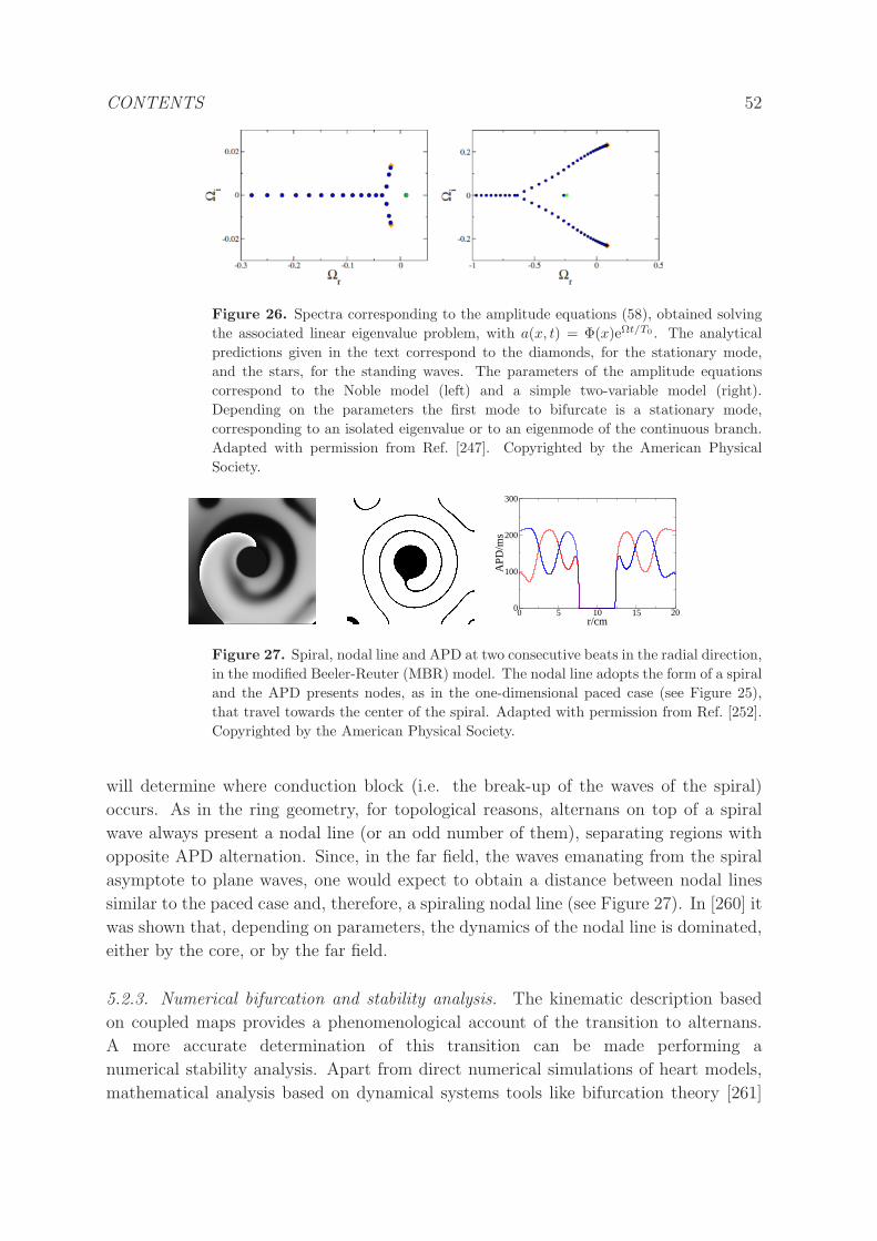
CONTENTS 52
Figure 26. Spectra corresponding to the amplitude equations (58), obtained solving
the associated linear eigenvalue problem, with a(x, t) = Φ(x)eΩt/T0 . The analytical
predictions given in the text correspond to the diamonds, for the stationary mode,
and the stars, for the standing waves. The parameters of the amplitude equations
correspond to the Noble model (left) and a simple two-variable model (right).
Depending on the parameters the first mode to bifurcate is a stationary mode,
corresponding to an isolated eigenvalue or to an eigenmode of the continuous branch.
Adapted with permission from Ref. [247]. Copyrighted by the American Physical
Society.
0 5 10 15 20r/cm
0
100
200
300A
PD/m
s
Figure 27. Spiral, nodal line and APD at two consecutive beats in the radial direction,
in the modified Beeler-Reuter (MBR) model. The nodal line adopts the form of a spiral
and the APD presents nodes, as in the one-dimensional paced case (see Figure 25),
that travel towards the center of the spiral. Adapted with permission from Ref. [252].
Copyrighted by the American Physical Society.
will determine where conduction block (i.e. the break-up of the waves of the spiral)
occurs. As in the ring geometry, for topological reasons, alternans on top of a spiral
wave always present a nodal line (or an odd number of them), separating regions with
opposite APD alternation. Since, in the far field, the waves emanating from the spiral
asymptote to plane waves, one would expect to obtain a distance between nodal lines
similar to the paced case and, therefore, a spiraling nodal line (see Figure 27). In [260] it
was shown that, depending on parameters, the dynamics of the nodal line is dominated,
either by the core, or by the far field.
5.2.3. Numerical bifurcation and stability analysis. The kinematic description based
on coupled maps provides a phenomenological account of the transition to alternans.
A more accurate determination of this transition can be made performing a
numerical stability analysis. Apart from direct numerical simulations of heart models,
mathematical analysis based on dynamical systems tools like bifurcation theory [261]
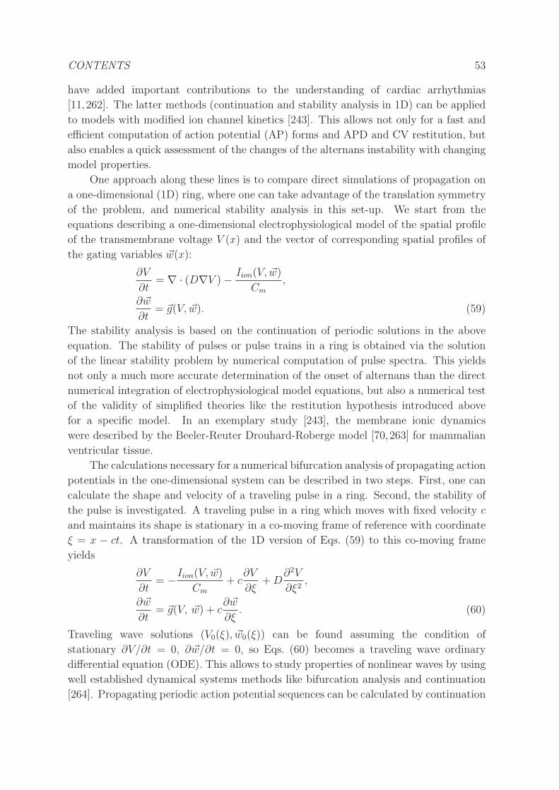
CONTENTS 53
have added important contributions to the understanding of cardiac arrhythmias
[11,262]. The latter methods (continuation and stability analysis in 1D) can be applied
to models with modified ion channel kinetics [243]. This allows not only for a fast and
efficient computation of action potential (AP) forms and APD and CV restitution, but
also enables a quick assessment of the changes of the alternans instability with changing
model properties.
One approach along these lines is to compare direct simulations of propagation on
a one-dimensional (1D) ring, where one can take advantage of the translation symmetry
of the problem, and numerical stability analysis in this set-up. We start from the
equations describing a one-dimensional electrophysiological model of the spatial profile
of the transmembrane voltage V (x) and the vector of corresponding spatial profiles of
the gating variables ~w(x):
∂V
∂t= ∇ · (D∇V )− Iion(V, ~w)
Cm
,
∂ ~w
∂t= ~g(V, ~w). (59)
The stability analysis is based on the continuation of periodic solutions in the above
equation. The stability of pulses or pulse trains in a ring is obtained via the solution
of the linear stability problem by numerical computation of pulse spectra. This yields
not only a much more accurate determination of the onset of alternans than the direct
numerical integration of electrophysiological model equations, but also a numerical test
of the validity of simplified theories like the restitution hypothesis introduced above
for a specific model. In an exemplary study [243], the membrane ionic dynamics
were described by the Beeler-Reuter Drouhard-Roberge model [70,263] for mammalian
ventricular tissue.
The calculations necessary for a numerical bifurcation analysis of propagating action
potentials in the one-dimensional system can be described in two steps. First, one can
calculate the shape and velocity of a traveling pulse in a ring. Second, the stability of
the pulse is investigated. A traveling pulse in a ring which moves with fixed velocity c
and maintains its shape is stationary in a co-moving frame of reference with coordinate
ξ = x − ct. A transformation of the 1D version of Eqs. (59) to this co-moving frame
yields
∂V
∂t= −Iion(V, ~w)
Cm
+ c∂V
∂ξ+D
∂2V
∂ξ2,
∂ ~w
∂t= ~g(V, ~w) + c
∂ ~w
∂ξ. (60)
Traveling wave solutions (V0(ξ), ~w0(ξ)) can be found assuming the condition of
stationary ∂V/∂t = 0, ∂ ~w/∂t = 0, so Eqs. (60) becomes a traveling wave ordinary
differential equation (ODE). This allows to study properties of nonlinear waves by using
well established dynamical systems methods like bifurcation analysis and continuation
[264]. Propagating periodic action potential sequences can be calculated by continuation
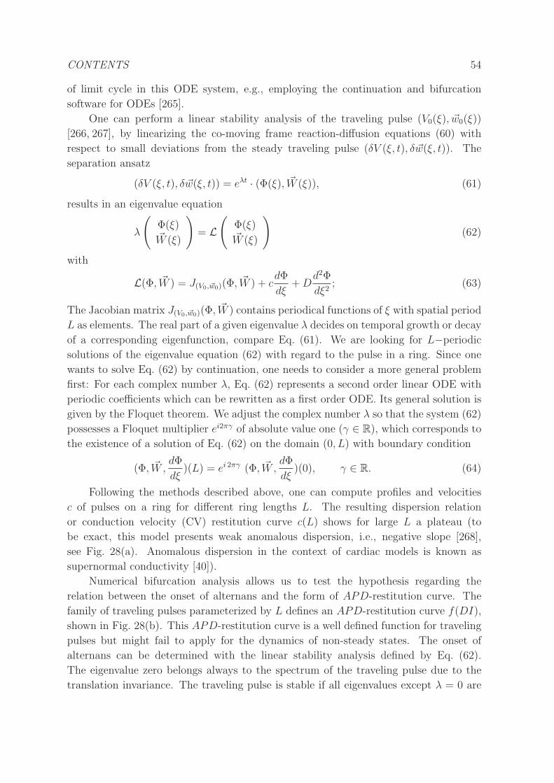
CONTENTS 54
of limit cycle in this ODE system, e.g., employing the continuation and bifurcation
software for ODEs [265].
One can perform a linear stability analysis of the traveling pulse (V0(ξ), ~w0(ξ))
[266, 267], by linearizing the co-moving frame reaction-diffusion equations (60) with
respect to small deviations from the steady traveling pulse (δV (ξ, t), δ ~w(ξ, t)). The
separation ansatz
(δV (ξ, t), δ ~w(ξ, t)) = eλt · (Φ(ξ), ~W (ξ)), (61)
results in an eigenvalue equation
λ
(
Φ(ξ)~W (ξ)
)
= L(
Φ(ξ)~W (ξ)
)
(62)
with
L(Φ, ~W ) = J(V0, ~w0)(Φ,~W ) + c
dΦ
dξ+D
d2Φ
dξ2; (63)
The Jacobian matrix J(V0, ~w0)(Φ,~W ) contains periodical functions of ξ with spatial period
L as elements. The real part of a given eigenvalue λ decides on temporal growth or decay
of a corresponding eigenfunction, compare Eq. (61). We are looking for L−periodic
solutions of the eigenvalue equation (62) with regard to the pulse in a ring. Since one
wants to solve Eq. (62) by continuation, one needs to consider a more general problem
first: For each complex number λ, Eq. (62) represents a second order linear ODE with
periodic coefficients which can be rewritten as a first order ODE. Its general solution is
given by the Floquet theorem. We adjust the complex number λ so that the system (62)
possesses a Floquet multiplier ei2πγ of absolute value one (γ ∈ R), which corresponds to
the existence of a solution of Eq. (62) on the domain (0, L) with boundary condition
(Φ, ~W,dΦ
dξ)(L) = ei 2πγ (Φ, ~W,
dΦ
dξ)(0), γ ∈ R. (64)
Following the methods described above, one can compute profiles and velocities
c of pulses on a ring for different ring lengths L. The resulting dispersion relation
or conduction velocity (CV) restitution curve c(L) shows for large L a plateau (to
be exact, this model presents weak anomalous dispersion, i.e., negative slope [268],
see Fig. 28(a). Anomalous dispersion in the context of cardiac models is known as
supernormal conductivity [40]).
Numerical bifurcation analysis allows us to test the hypothesis regarding the
relation between the onset of alternans and the form of APD-restitution curve. The
family of traveling pulses parameterized by L defines an APD-restitution curve f(DI),
shown in Fig. 28(b). This APD-restitution curve is a well defined function for traveling
pulses but might fail to apply for the dynamics of non-steady states. The onset of
alternans can be determined with the linear stability analysis defined by Eq. (62).
The eigenvalue zero belongs always to the spectrum of the traveling pulse due to the
translation invariance. The traveling pulse is stable if all eigenvalues except λ = 0 are
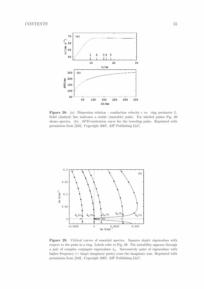
CONTENTS 55
Figure 28. (a): Dispersion relation - conduction velocity c vs. ring perimeter L.
Solid (dashed) line indicates a stable (unstable) pulse. For labeled pulses Fig. 29
shows spectra. (b): APD-restitution curve for the traveling pulse. Reprinted with
permission from [243]. Copyright 2007, AIP Publishing LLC.
Figure 29. Critical curves of essential spectra. Squares depict eigenvalues with
respect to the pulse in a ring. Labels refer to Fig. 28. The instability appears through
a pair of complex conjugate eigenvalues λa. Successively pairs of eigenvalues with
higher frequency (= larger imaginary parts) cross the imaginary axis. Reprinted with
permission from [243]. Copyright 2007, AIP Publishing LLC.
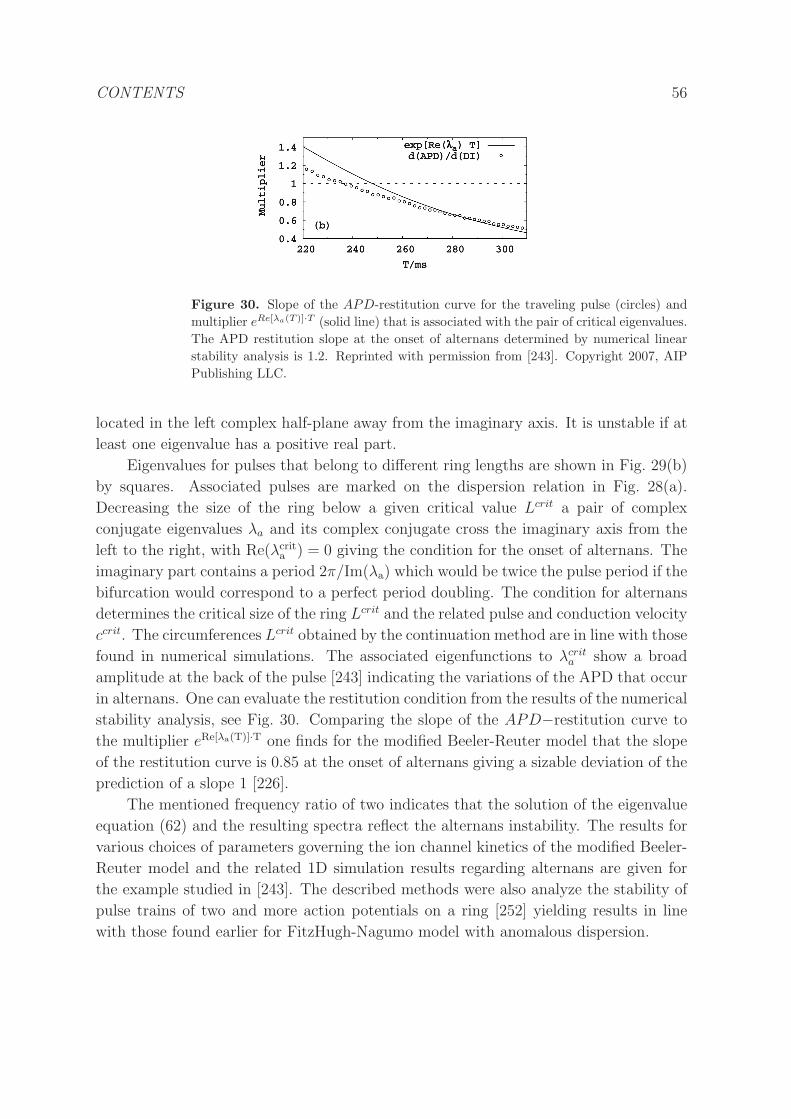
CONTENTS 56
Figure 30. Slope of the APD-restitution curve for the traveling pulse (circles) and
multiplier eRe[λa(T )]·T (solid line) that is associated with the pair of critical eigenvalues.
The APD restitution slope at the onset of alternans determined by numerical linear
stability analysis is 1.2. Reprinted with permission from [243]. Copyright 2007, AIP
Publishing LLC.
located in the left complex half-plane away from the imaginary axis. It is unstable if at
least one eigenvalue has a positive real part.
Eigenvalues for pulses that belong to different ring lengths are shown in Fig. 29(b)
by squares. Associated pulses are marked on the dispersion relation in Fig. 28(a).
Decreasing the size of the ring below a given critical value Lcrit a pair of complex
conjugate eigenvalues λa and its complex conjugate cross the imaginary axis from the
left to the right, with Re(λcrita ) = 0 giving the condition for the onset of alternans. The
imaginary part contains a period 2π/Im(λa) which would be twice the pulse period if the
bifurcation would correspond to a perfect period doubling. The condition for alternans
determines the critical size of the ring Lcrit and the related pulse and conduction velocity
ccrit. The circumferences Lcrit obtained by the continuation method are in line with those
found in numerical simulations. The associated eigenfunctions to λcrita show a broad
amplitude at the back of the pulse [243] indicating the variations of the APD that occur
in alternans. One can evaluate the restitution condition from the results of the numerical
stability analysis, see Fig. 30. Comparing the slope of the APD−restitution curve to
the multiplier eRe[λa(T)]·T one finds for the modified Beeler-Reuter model that the slope
of the restitution curve is 0.85 at the onset of alternans giving a sizable deviation of the
prediction of a slope 1 [226].
The mentioned frequency ratio of two indicates that the solution of the eigenvalue
equation (62) and the resulting spectra reflect the alternans instability. The results for
various choices of parameters governing the ion channel kinetics of the modified Beeler-
Reuter model and the related 1D simulation results regarding alternans are given for
the example studied in [243]. The described methods were also analyze the stability of
pulse trains of two and more action potentials on a ring [252] yielding results in line
with those found earlier for FitzHugh-Nagumo model with anomalous dispersion.
CONTENTS 57
6. Spiral wave dynamics
Rotating excitations (rotors) are often found in cardiac experiments and corresponding
simulations. A special case of two-dimensional rotors are spiral waves, that are discussed
in this section. Their three-dimensional equivalent are scroll waves that will be reviewed
separately in the next section. Spirals can become unstable (spiral breakup), which leads
typically to a state of irregular, chaotic activity. The description of reentry in cardiac
tissue in terms of a rotating wave around an obstacle forming a spiral wave dates back
to a classical paper by Wiener and Rosenblueth in 1946 [269]. Later, it was shown in
chemical media (i.e., in the Belousov-Zhabotinsky (BZ) reaction [270]) that such rotors
can be autonomous and circulate around an unexcited area referred to as the spiral
core. An obstacle is thus not necessary to sustain spiral waves in excitable media. In
the cardiac literature this latter case is refered to as functional reentry, and contrasted
with anatomical reentry when the spiral wave is anchored to an obstacle and rotates
around a region of heterogeneous tissue. In any of these cases, the rotors impose a
frequency that is much larger than the natural sinus rhythm frequency of the heart
and are therefore widely discussed as building block of ventricular tachycardias and
fibrillation, see e. g. [20]. To exist, sustained rotating spirals need a minimum system
size of 20 percent of the spiral wavelength in an unbounded domain. So one may expect
that rotors are not found in small animals. Recent studies, however, reveal that (stable
and unstable) spirals and the related signature of ventricular fibrillation (VF) appear
even in mice and rats. A comparative analysis of typical VF frequencies νV F in animals
from mice and rats via cats, dogs and pigs to humans and horses displays a characteristic
power law scaling with νV F ∝ BM−1/4, where BM is the body mass [271]. Similarly,
the rotor core diameter R scales with R ∝ BM1/4, while the action potential velocity is
practically constant. In absolute numbers, characteristic fibrillation frequencies decrease
from 38 Hz in mice to 6.8 Hz in humans. Since the extension L of the heart roughly
scales with L ∝ BM1/4, the characteristic ratio of system size L to rotor size R is only
weakly dependent on the size of the animal and apart from the characteristic scaling of
frequencies and lengths comparable rotor dynamics may be observed in many different
species.
Theoretical analysis and numerical simulations of spirals in cardiac propagation
were often motivated by the rich variety of experimentally observed spiral dynamics.
Stationary and drifting spirals were discovered, e. g., in slices of ventricular muscle
from dog and sheep [16, 17]. Later on, improved imaging techniques allowed the
visualization of spiral dynamics on the surface of isolated rabbit hearts [135], wherein
nonstationary reentrant spiral dynamics was identified as a mechanism for polymorphic
tachycardia. Optical imaging of electrical activity in isolated, perfused dog hearts
enabled the observation of transiently erupting rotors and frequent wavefront collisions
and wavebreak generation in the early phase of ventricular fibrillation-like activity [272].
In parallel, a method to obtain spatial phase maps (i.e., representation of the dynamical
phase of the local excitations, see Fig.2) was developed that allowed to identify the

CONTENTS 58
Figure 31. Types of spiral wave dynamics in numerical simulations of the Fenton-
Karma model together with the trajectory of the spiral tip, and its relation to cardiac
arrhythmia: Monomorphic ventricular tachycardia related with a rigid rotating spiral
wave (a), polymorphic ventricular tachycardia related with a meandering spiral wave
(b) and ventricular fibrillation related with spiral breakup (c).
multiple spiral tips (i.e., phase singularities), as sources of fibrillatory activity and
rotating, reentrant excitations and to follow their temporal evolution with emphasis
on formation and termination of such rotors [273].
Depending on the dynamics of the tip and the type of wave interaction between
consecutive pulses of the same spiral wave, different types of behavior are observed, see
Fig. 31 for three representative examples:
• Rigidly rotating spiral waves: the tip of the spiral wave rotates rigidly around
a circular unexcited region, the core (Fig. 31(a)). Under some conditions such
dynamics is associated with monomorphic ventricular tachycardia where the ECG
shows a fast characteristic frequency [17]. Two limiting cases can be distinguished:
the large core regime, when the core size is larger than the typical spiral wavelength
and there is not interaction between consecutive pulses, and the small core regime,
where the core size is much smaller than the wavelength [274].
• Meandering spiral waves: the motion of the tip is not circular but it performs
a more complex motion. These spiral waves would produce the appearance of
several frequencies in the ECG and, therefore, they are associated to polymorphic
ventricular tachycardia. In the simplest case two frequencies are combined to
produce epicycloid or hypocycloid dynamics [275]. The appearance of additional
frequencies produces complex spiral motion [276]. In effect, the typical spiral waves
observed in models of cardiac tissue present elongated cores. In these, the tip
follows a relatively large straight motion along the refractory tail of the previous
pulse combined with rapid turns (Fig. 31(b)) [277]. Variation of parameters in
cardiac models yields a variety of meander patterns [74].
• Spiral break-up: the interaction between pulses can produce the breaking of the
spiral in different pieces that automatically rotate and produce new spiral waves.
Then, the new spirals break again, producing a cascade effect (Fig. 31(c)). A final
chaotic dynamic state of pieces of rotating spirals fills out the whole system [91,278].
Such a state has been proposed to underlie ventricular and atrial fibrillation [80,279].
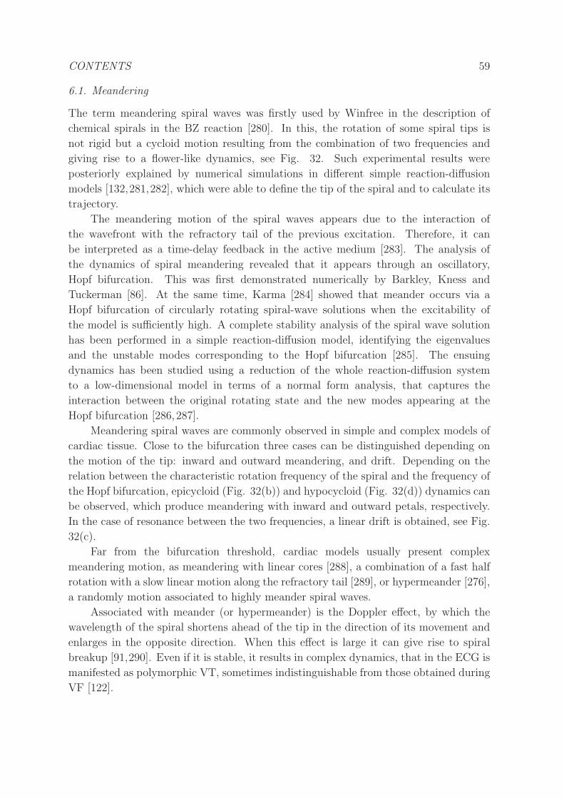
CONTENTS 59
6.1. Meandering
The term meandering spiral waves was firstly used by Winfree in the description of
chemical spirals in the BZ reaction [280]. In this, the rotation of some spiral tips is
not rigid but a cycloid motion resulting from the combination of two frequencies and
giving rise to a flower-like dynamics, see Fig. 32. Such experimental results were
posteriorly explained by numerical simulations in different simple reaction-diffusion
models [132,281,282], which were able to define the tip of the spiral and to calculate its
trajectory.
The meandering motion of the spiral waves appears due to the interaction of
the wavefront with the refractory tail of the previous excitation. Therefore, it can
be interpreted as a time-delay feedback in the active medium [283]. The analysis of
the dynamics of spiral meandering revealed that it appears through an oscillatory,
Hopf bifurcation. This was first demonstrated numerically by Barkley, Kness and
Tuckerman [86]. At the same time, Karma [284] showed that meander occurs via a
Hopf bifurcation of circularly rotating spiral-wave solutions when the excitability of
the model is sufficiently high. A complete stability analysis of the spiral wave solution
has been performed in a simple reaction-diffusion model, identifying the eigenvalues
and the unstable modes corresponding to the Hopf bifurcation [285]. The ensuing
dynamics has been studied using a reduction of the whole reaction-diffusion system
to a low-dimensional model in terms of a normal form analysis, that captures the
interaction between the original rotating state and the new modes appearing at the
Hopf bifurcation [286,287].
Meandering spiral waves are commonly observed in simple and complex models of
cardiac tissue. Close to the bifurcation three cases can be distinguished depending on
the motion of the tip: inward and outward meandering, and drift. Depending on the
relation between the characteristic rotation frequency of the spiral and the frequency of
the Hopf bifurcation, epicycloid (Fig. 32(b)) and hypocycloid (Fig. 32(d)) dynamics can
be observed, which produce meandering with inward and outward petals, respectively.
In the case of resonance between the two frequencies, a linear drift is obtained, see Fig.
32(c).
Far from the bifurcation threshold, cardiac models usually present complex
meandering motion, as meandering with linear cores [288], a combination of a fast half
rotation with a slow linear motion along the refractory tail [289], or hypermeander [276],
a randomly motion associated to highly meander spiral waves.
Associated with meander (or hypermeander) is the Doppler effect, by which the
wavelength of the spiral shortens ahead of the tip in the direction of its movement and
enlarges in the opposite direction. When this effect is large it can give rise to spiral
breakup [91,290]. Even if it is stable, it results in complex dynamics, that in the ECG is
manifested as polymorphic VT, sometimes indistinguishable from those obtained during
VF [122].
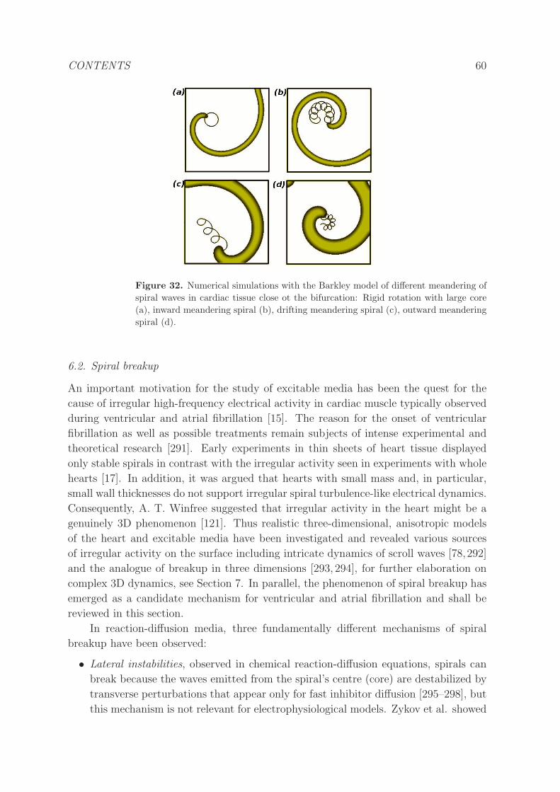
CONTENTS 60
Figure 32. Numerical simulations with the Barkley model of different meandering of
spiral waves in cardiac tissue close ot the bifurcation: Rigid rotation with large core
(a), inward meandering spiral (b), drifting meandering spiral (c), outward meandering
spiral (d).
6.2. Spiral breakup
An important motivation for the study of excitable media has been the quest for the
cause of irregular high-frequency electrical activity in cardiac muscle typically observed
during ventricular and atrial fibrillation [15]. The reason for the onset of ventricular
fibrillation as well as possible treatments remain subjects of intense experimental and
theoretical research [291]. Early experiments in thin sheets of heart tissue displayed
only stable spirals in contrast with the irregular activity seen in experiments with whole
hearts [17]. In addition, it was argued that hearts with small mass and, in particular,
small wall thicknesses do not support irregular spiral turbulence-like electrical dynamics.
Consequently, A. T. Winfree suggested that irregular activity in the heart might be a
genuinely 3D phenomenon [121]. Thus realistic three-dimensional, anisotropic models
of the heart and excitable media have been investigated and revealed various sources
of irregular activity on the surface including intricate dynamics of scroll waves [78,292]
and the analogue of breakup in three dimensions [293, 294], for further elaboration on
complex 3D dynamics, see Section 7. In parallel, the phenomenon of spiral breakup has
emerged as a candidate mechanism for ventricular and atrial fibrillation and shall be
reviewed in this section.
In reaction-diffusion media, three fundamentally different mechanisms of spiral
breakup have been observed:
• Lateral instabilities, observed in chemical reaction-diffusion equations, spirals can
break because the waves emitted from the spiral’s centre (core) are destabilized by
transverse perturbations that appear only for fast inhibitor diffusion [295–298], but
this mechanism is not relevant for electrophysiological models. Zykov et al. showed
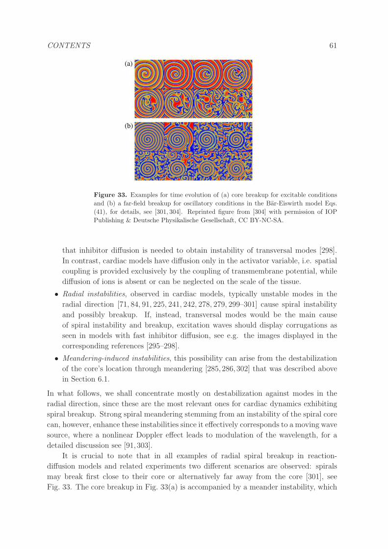
CONTENTS 61
Figure 33. Examples for time evolution of (a) core breakup for excitable conditions
and (b) a far-field breakup for oscillatory conditions in the Bar-Eiswirth model Eqs.
(41), for details, see [301, 304]. Reprinted figure from [304] with permission of IOP
Publishing & Deutsche Physikalische Gesellschaft, CC BY-NC-SA.
that inhibitor diffusion is needed to obtain instability of transversal modes [298].
In contrast, cardiac models have diffusion only in the activator variable, i.e. spatial
coupling is provided exclusively by the coupling of transmembrane potential, while
diffusion of ions is absent or can be neglected on the scale of the tissue.
• Radial instabilities, observed in cardiac models, typically unstable modes in the
radial direction [71, 84, 91, 225, 241, 242, 278, 279, 299–301] cause spiral instability
and possibly breakup. If, instead, transversal modes would be the main cause
of spiral instability and breakup, excitation waves should display corrugations as
seen in models with fast inhibitor diffusion, see e.g. the images displayed in the
corresponding references [295–298].
• Meandering-induced instabilities, this possibility can arise from the destabilization
of the core’s location through meandering [285, 286, 302] that was described above
in Section 6.1.
In what follows, we shall concentrate mostly on destabilization against modes in the
radial direction, since these are the most relevant ones for cardiac dynamics exhibiting
spiral breakup. Strong spiral meandering stemming from an instability of the spiral core
can, however, enhance these instabilities since it effectively corresponds to a moving wave
source, where a nonlinear Doppler effect leads to modulation of the wavelength, for a
detailed discussion see [91, 303].
It is crucial to note that in all examples of radial spiral breakup in reaction-
diffusion models and related experiments two different scenarios are observed: spirals
may break first close to their core or alternatively far away from the core [301], see
Fig. 33. The core breakup in Fig. 33(a) is accompanied by a meander instability, which
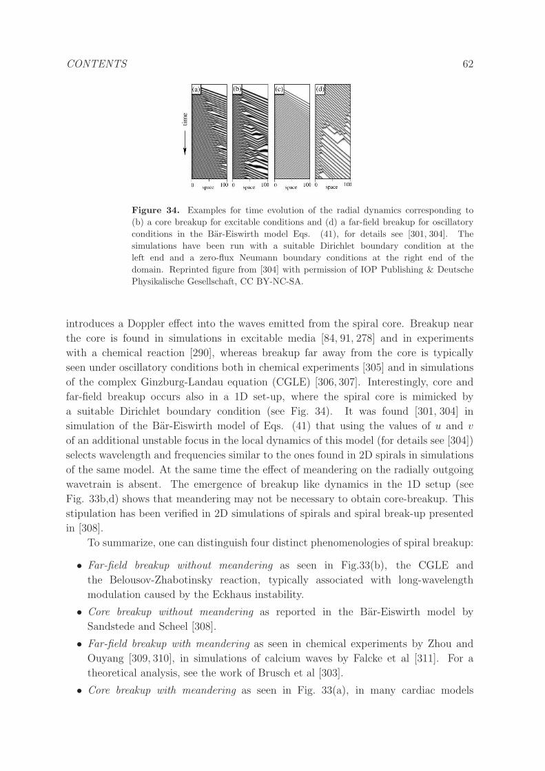
CONTENTS 62
Figure 34. Examples for time evolution of the radial dynamics corresponding to
(b) a core breakup for excitable conditions and (d) a far-field breakup for oscillatory
conditions in the Bar-Eiswirth model Eqs. (41), for details see [301, 304]. The
simulations have been run with a suitable Dirichlet boundary condition at the
left end and a zero-flux Neumann boundary conditions at the right end of the
domain. Reprinted figure from [304] with permission of IOP Publishing & Deutsche
Physikalische Gesellschaft, CC BY-NC-SA.
introduces a Doppler effect into the waves emitted from the spiral core. Breakup near
the core is found in simulations in excitable media [84, 91, 278] and in experiments
with a chemical reaction [290], whereas breakup far away from the core is typically
seen under oscillatory conditions both in chemical experiments [305] and in simulations
of the complex Ginzburg-Landau equation (CGLE) [306, 307]. Interestingly, core and
far-field breakup occurs also in a 1D set-up, where the spiral core is mimicked by
a suitable Dirichlet boundary condition (see Fig. 34). It was found [301, 304] in
simulation of the Bar-Eiswirth model of Eqs. (41) that using the values of u and v
of an additional unstable focus in the local dynamics of this model (for details see [304])
selects wavelength and frequencies similar to the ones found in 2D spirals in simulations
of the same model. At the same time the effect of meandering on the radially outgoing
wavetrain is absent. The emergence of breakup like dynamics in the 1D setup (see
Fig. 33b,d) shows that meandering may not be necessary to obtain core-breakup. This
stipulation has been verified in 2D simulations of spirals and spiral break-up presented
in [308].
To summarize, one can distinguish four distinct phenomenologies of spiral breakup:
• Far-field breakup without meandering as seen in Fig.33(b), the CGLE and
the Belousov-Zhabotinsky reaction, typically associated with long-wavelength
modulation caused by the Eckhaus instability.
• Core breakup without meandering as reported in the Bar-Eiswirth model by
Sandstede and Scheel [308].
• Far-field breakup with meandering as seen in chemical experiments by Zhou and
Ouyang [309, 310], in simulations of calcium waves by Falcke et al [311]. For a
theoretical analysis, see the work of Brusch et al [303].
• Core breakup with meandering as seen in Fig. 33(a), in many cardiac models
CONTENTS 63
[84, 279, 292] and in experiments with the Belousov-Zhabotinsky reaction [310].
This route is often termed Doppler-induced instability.
For models of cardiac tissue, usually core-breakup and strong meandering of the
spiral core is observed [279].
CONTENTS 64
7. Scroll wave dynamics
In the ventricles, one has to take into account that the wall thickness is not negligible,
making the tissue fully three-dimensional. The natural extension of spiral waves in two
dimensions corresponds to scroll waves in three dimensions.
Straight scroll waves may rotate with constant frequency. However, under certain
conditions the filament of the scroll is not straight but takes a helical shape under
meandering, see Section 7.1, or when an external twist is imposed, see Section 7.2; or it
may produce complex unstable dynamics if the tension of the filament is negative, see
Section 7.3. Finally, the breakup of spiral and of scroll waves are discussed in Section
7.4.
7.1. Meandering
The natural extension of two-dimensional meandering to more realistic three-
dimensional tissue is the meandering of scroll waves [312]. The first explicit simulations
of scroll meandering were obtained with simple models and its dynamics employed to
explain relevant properties of the ECG under arrhythmic conditions [135].
In the first numerical simulations an equivalent behavior to two-dimensional
meandering was assumed. However, it was observed that scroll curvature modifies the
meander Hopf instability, resulting in a short wavelength instability that saturates.
Then, one obtains helicoidal meandering scrolls [313] because the meandering of the
filament of the scroll wave promotes the bending of the filament [73].
The linear stability analysis of scroll waves shows that the branch of meander modes
can become unstable for finite wavelength perturbations along the filament, see Sec.
8.2.2, even if it is stable in two dimensions, so three-dimensional effects make the scroll
unstable where the spiral was stable [139,314]. The final nonlinear state depends on the
boundary conditions, so the amplitude of meander is constant along the direction of the
filament z for periodic boundary conditions, but varies with z for non-flux boundary
conditions.
Spiral meander in the presence of an external field can be studied using a normal
form model [315], which can also be applied to a scroll wave, with filament curvature
taking the place of the external field. This improves previous models [313] by considering
the effect of scroll curvature both in the motion of the instantaneous filament and in
the amplitude of the meander modes and explains the difference in curvature between
the translation and meander modes.
Apart from the quasi two-dimensional periodic meander, complex aperiodic
meander has also been described [316], which presents buckling of the scroll wave, an
instability typically associated to negative filament tension, see Sec.7.3.2.
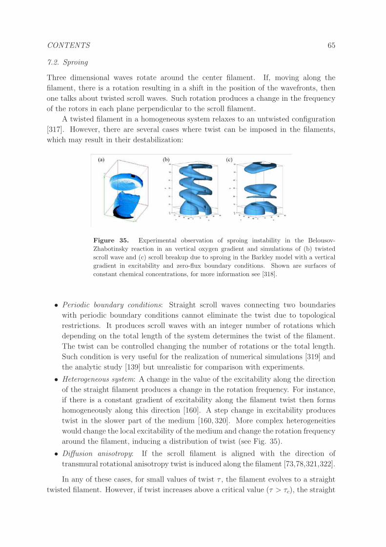
CONTENTS 65
7.2. Sproing
Three dimensional waves rotate around the center filament. If, moving along the
filament, there is a rotation resulting in a shift in the position of the wavefronts, then
one talks about twisted scroll waves. Such rotation produces a change in the frequency
of the rotors in each plane perpendicular to the scroll filament.
A twisted filament in a homogeneous system relaxes to an untwisted configuration
[317]. However, there are several cases where twist can be imposed in the filaments,
which may result in their destabilization:
Figure 35. Experimental observation of sproing instability in the Belousov-
Zhabotinsky reaction in an vertical oxygen gradient and simulations of (b) twisted
scroll wave and (c) scroll breakup due to sproing in the Barkley model with a vertical
gradient in excitability and zero-flux boundary conditions. Shown are surfaces of
constant chemical concentrations, for more information see [318].
• Periodic boundary conditions: Straight scroll waves connecting two boundaries
with periodic boundary conditions cannot eliminate the twist due to topological
restrictions. It produces scroll waves with an integer number of rotations which
depending on the total length of the system determines the twist of the filament.
The twist can be controlled changing the number of rotations or the total length.
Such condition is very useful for the realization of numerical simulations [319] and
the analytic study [139] but unrealistic for comparison with experiments.
• Heterogeneous system: A change in the value of the excitability along the direction
of the straight filament produces a change in the rotation frequency. For instance,
if there is a constant gradient of excitability along the filament twist then forms
homogeneously along this direction [160]. A step change in excitability produces
twist in the slower part of the medium [160, 320]. More complex heterogeneities
would change the local excitability of the medium and change the rotation frequency
around the filament, inducing a distribution of twist (see Fig. 35).
• Diffusion anisotropy: If the scroll filament is aligned with the direction of
transmural rotational anisotropy twist is induced along the filament [73,78,321,322].
In any of these cases, for small values of twist τ , the filament evolves to a straight
twisted filament. However, if twist increases above a critical value (τ > τc), the straight
CONTENTS 66
filament becomes unstable giving rise to a helical shape of the filament [139], in an
instability known as sproing. The radius of the helix grows as the square root of the
difference between the actual twist value and the critical value (√τ − τc), which suggests
that it corresponds to a supercitical Hopf bifurcation.
7.3. Negative line tension
Even if the scroll filaments are just convenient mathematical entities, their dynamics
permits to assign them physical magnitudes like tension. The first reference to the
concept of filament tension of scroll waves is due to Yakushevich [323].
The first three-dimensional numerical simulations showed the dynamics of scroll
waves with positive filament tension: straight filaments are stable while scroll rings
shrink and disappear [324]. Then, numerical simulations were done showing not
only shrink of scroll rings but also expansion [92]. Almost simultaneously, the first
interpretations in terms of kinematic theory already predicted the existence of expanding
scroll rings [325], implying that a straight scroll wave had to be also unstable.
The first clear numerical simulations of negative filament tension where done by
Biktashev et al and the instability explained in terms of negative filament tension using
a perturbation theory [93]. Recently, Dierckx et al [326] have calculated higher orders
in the perturbation theory in generic models of excitable media.
Numerically, the full turbulent dynamics was studied some years later [140] and its
possible appearance in ionic models of cardiac tissue was also discussed [75], where it is
related to reduced conductances of sodium and slow inward currents. These low values
are typically employed to model ischemic conditions of cardiac tissue [126].
Further understanding of this instability was obtained when, using a complete linear
stability analysis of the scroll wave solution in a simple reaction-diffusion model, the
unstable mode corresponding to the negative filament instability was identified as a
translational mode, related to rigid body displacements in the direction perpendicular
to the filament [314].
In simple models positive tension occurs for a medium with high excitability,
i.e. a low excitation threshold, while negative tension occurs typically in media with
low excitability [40, 140, 325]. However, more elaborate models show a region of the
parameter space where scroll rings can slowly expand even if the medium is highly
excitable [327], although turbulent dynamics was not observed in such simulations.
Besides a change in the parameters of the model, the excitability of the medium can also
be decreased replacing the partial differential equations by a discrete model, resulting
in a change of filament tension when discreteness is increased [192].
The most detailed study of the onset of negative filament tension has been
performed in the Barkley model Eqs. (40) [139,140,328]. In a large region of parameters
Eqs. (40) produce stable scroll waves with positive tension and without any scroll
breakup, see Fig. 36. Negative filament tension appears inside a broad region of
parameters and closer to the non-excitable condition, where free edges retract, see
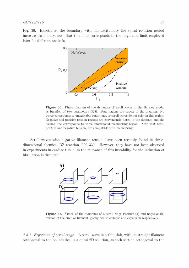
CONTENTS 67
Fig. 36. Exactly at the boundary with non-excitability the spiral rotation period
increases to infinity, note that this limit corresponds to the large core limit employed
later for different analysis.
0,4 0,6 0,8 1p
1
0
0,1
0,2
p2
No Waves
Negative
PositivetensionMeandering
tension
Figure 36. Phase diagram of the dynamics of scroll waves in the Barkley model
as function of two parameters [328]. Four regions are shown in the diagram: No
waves corresponds to unexcitable conditions, so scroll waves do not exist in this region;
Negative and positive tension regions are conveniently noted in the diagram and the
dashed line corresponds to three-dimensional meandering region. Note that both,
positive and negative tension, are compatible with meandering.
Scroll waves with negative filament tension have been recently found in three-
dimensional chemical BZ reaction [329, 330]. However, they have not been observed
in experiments in cardiac tissue, so the relevance of this instability for the induction of
fibrillation is disputed.
Figure 37. Sketch of the dynamics of a scroll ring: Positive (a) and negative (b)
tension of the circular filament, giving rise to collapse and expansion respectively.
7.3.1. Expansion of scroll rings. A scroll wave in a thin slab, with its straight filament
orthogonal to the boundaries, is a quasi 2D solution, as each section orthogonal to the
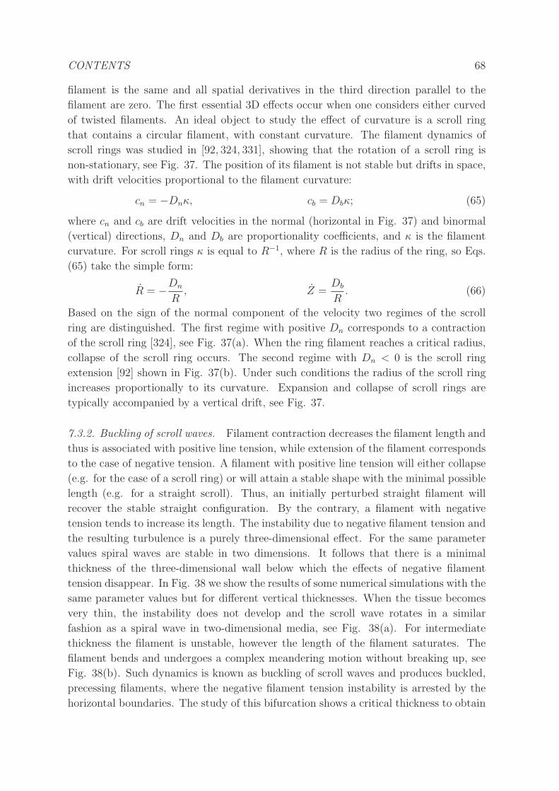
CONTENTS 68
filament is the same and all spatial derivatives in the third direction parallel to the
filament are zero. The first essential 3D effects occur when one considers either curved
of twisted filaments. An ideal object to study the effect of curvature is a scroll ring
that contains a circular filament, with constant curvature. The filament dynamics of
scroll rings was studied in [92, 324, 331], showing that the rotation of a scroll ring is
non-stationary, see Fig. 37. The position of its filament is not stable but drifts in space,
with drift velocities proportional to the filament curvature:
cn = −Dnκ, cb = Dbκ; (65)
where cn and cb are drift velocities in the normal (horizontal in Fig. 37) and binormal
(vertical) directions, Dn and Db are proportionality coefficients, and κ is the filament
curvature. For scroll rings κ is equal to R−1, where R is the radius of the ring, so Eqs.
(65) take the simple form:
R = −Dn
R, Z =
Db
R. (66)
Based on the sign of the normal component of the velocity two regimes of the scroll
ring are distinguished. The first regime with positive Dn corresponds to a contraction
of the scroll ring [324], see Fig. 37(a). When the ring filament reaches a critical radius,
collapse of the scroll ring occurs. The second regime with Dn < 0 is the scroll ring
extension [92] shown in Fig. 37(b). Under such conditions the radius of the scroll ring
increases proportionally to its curvature. Expansion and collapse of scroll rings are
typically accompanied by a vertical drift, see Fig. 37.
7.3.2. Buckling of scroll waves. Filament contraction decreases the filament length and
thus is associated with positive line tension, while extension of the filament corresponds
to the case of negative tension. A filament with positive line tension will either collapse
(e.g. for the case of a scroll ring) or will attain a stable shape with the minimal possible
length (e.g. for a straight scroll). Thus, an initially perturbed straight filament will
recover the stable straight configuration. By the contrary, a filament with negative
tension tends to increase its length. The instability due to negative filament tension and
the resulting turbulence is a purely three-dimensional effect. For the same parameter
values spiral waves are stable in two dimensions. It follows that there is a minimal
thickness of the three-dimensional wall below which the effects of negative filament
tension disappear. In Fig. 38 we show the results of some numerical simulations with the
same parameter values but for different vertical thicknesses. When the tissue becomes
very thin, the instability does not develop and the scroll wave rotates in a similar
fashion as a spiral wave in two-dimensional media, see Fig. 38(a). For intermediate
thickness the filament is unstable, however the length of the filament saturates. The
filament bends and undergoes a complex meandering motion without breaking up, see
Fig. 38(b). Such dynamics is known as buckling of scroll waves and produces buckled,
precessing filaments, where the negative filament tension instability is arrested by the
horizontal boundaries. The study of this bifurcation shows a critical thickness to obtain
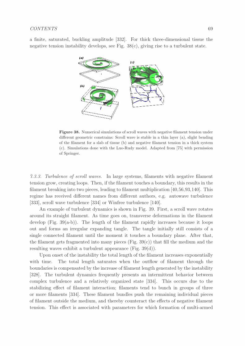
CONTENTS 69
a finite, saturated, buckling amplitude [332]. For thick three-dimensional tissue the
negative tension instability develops, see Fig. 38(c), giving rise to a turbulent state.
Figure 38. Numerical simulations of scroll waves with negative filament tension under
different geometric constrains: Scroll wave is stable in a thin layer (a), slight bending
of the filament for a slab of tissue (b) and negative filament tension in a thick system
(c). Simulations done with the Luo-Rudy model. Adapted from [75] with permission
of Springer.
7.3.3. Turbulence of scroll waves. In large systems, filaments with negative filament
tension grow, creating loops. Then, if the filament touches a boundary, this results in the
filament breaking into two pieces, leading to filament multiplication [40,56,93,140]. This
regime has received different names from different authors, e.g. autowave turbulence
[333], scroll wave turbulence [334] or Winfree turbulence [140].
An example of turbulent dynamics is shown in Fig. 39. First, a scroll wave rotates
around its straight filament. As time goes on, transverse deformations in the filament
develop (Fig. 39(a-b)). The length of the filament rapidly increases because it loops
out and forms an irregular expanding tangle. The tangle initially still consists of a
single connected filament until the moment it touches a boundary plane. After that,
the filament gets fragmented into many pieces (Fig. 39(c)) that fill the medium and the
resulting waves exhibit a turbulent appearance (Fig. 39(d)).
Upon onset of the instability the total length of the filament increases exponentially
with time. The total length saturates when the outflow of filament through the
boundaries is compensated by the increase of filament length generated by the instability
[328]. The turbulent dynamics frequently presents an intermittent behavior between
complex turbulence and a relatively organized state [334]. This occurs due to the
stabilizing effect of filament interaction; filaments tend to bunch in groups of three
or more filaments [334]. These filament bundles push the remaining individual pieces
of filament outside the medium, and thereby counteract the effects of negative filament
tension. This effect is associated with parameters for which formation of multi-armed
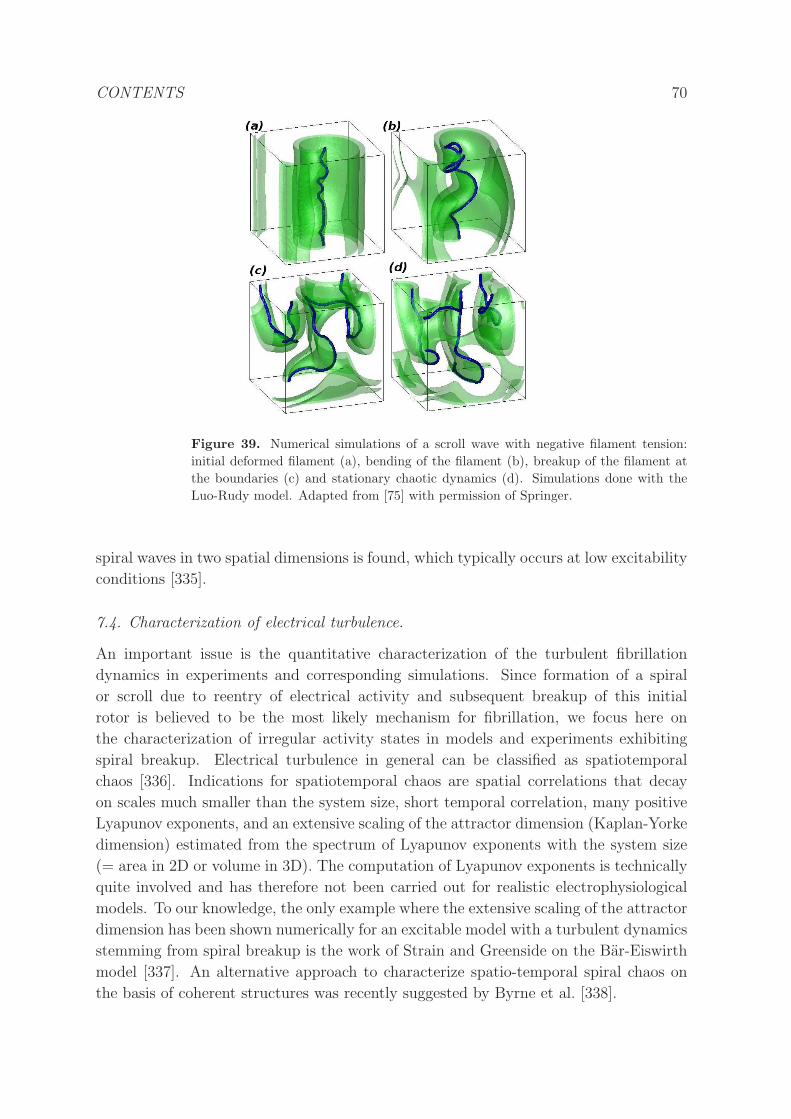
CONTENTS 70
Figure 39. Numerical simulations of a scroll wave with negative filament tension:
initial deformed filament (a), bending of the filament (b), breakup of the filament at
the boundaries (c) and stationary chaotic dynamics (d). Simulations done with the
Luo-Rudy model. Adapted from [75] with permission of Springer.
spiral waves in two spatial dimensions is found, which typically occurs at low excitability
conditions [335].
7.4. Characterization of electrical turbulence.
An important issue is the quantitative characterization of the turbulent fibrillation
dynamics in experiments and corresponding simulations. Since formation of a spiral
or scroll due to reentry of electrical activity and subsequent breakup of this initial
rotor is believed to be the most likely mechanism for fibrillation, we focus here on
the characterization of irregular activity states in models and experiments exhibiting
spiral breakup. Electrical turbulence in general can be classified as spatiotemporal
chaos [336]. Indications for spatiotemporal chaos are spatial correlations that decay
on scales much smaller than the system size, short temporal correlation, many positive
Lyapunov exponents, and an extensive scaling of the attractor dimension (Kaplan-Yorke
dimension) estimated from the spectrum of Lyapunov exponents with the system size
(= area in 2D or volume in 3D). The computation of Lyapunov exponents is technically
quite involved and has therefore not been carried out for realistic electrophysiological
models. To our knowledge, the only example where the extensive scaling of the attractor
dimension has been shown numerically for an excitable model with a turbulent dynamics
stemming from spiral breakup is the work of Strain and Greenside on the Bar-Eiswirth
model [337]. An alternative approach to characterize spatio-temporal spiral chaos on
the basis of coherent structures was recently suggested by Byrne et al. [338].
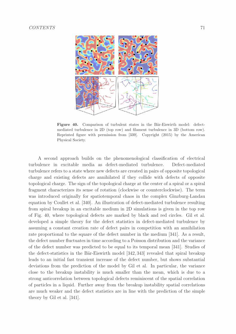
CONTENTS 71
Figure 40. Comparison of turbulent states in the Bar-Eiswirth model: defect-
mediated turbulence in 2D (top row) and filament turbulence in 3D (bottom row).
Reprinted figure with permission from [339]. Copyright (2015) by the American
Physical Society.
A second approach builds on the phenomenological classification of electrical
turbulence in excitable media as defect-mediated turbulence. Defect-mediated
turbulence refers to a state where new defects are created in pairs of opposite topological
charge and existing defects are annihilated if they collide with defects of opposite
topological charge. The sign of the topological charge at the center of a spiral or a spiral
fragment characterizes its sense of rotation (clockwise or counterclockwise). The term
was introduced originally for spatiotemporal chaos in the complex Ginzburg-Landau
equation by Coullet et al. [340]. An illustration of defect-mediated turbulence resulting
from spiral breakup in an excitable medium in 2D simulations is given in the top row
of Fig. 40, where topological defects are marked by black and red circles. Gil et al.
developed a simple theory for the defect statistics in defect-mediated turbulence by
assuming a constant creation rate of defect pairs in competition with an annihilation
rate proportional to the square of the defect number in the medium [341]. As a result,
the defect number fluctuates in time according to a Poisson distribution and the variance
of the defect number was predicted to be equal to its temporal mean [341]. Studies of
the defect-statistics in the Bar-Eiswirth model [342, 343] revealed that spiral breakup
leads to an initial fast transient increase of the defect number, but shows substantial
deviations from the prediction of the model by Gil et al. In particular, the variance
close to the breakup instability is much smaller than the mean, which is due to a
strong anticorrelation between topological defects reminiscent of the spatial correlation
of particles in a liquid. Further away from the breakup instability spatial correlations
are much weaker and the defect statistics are in line with the prediction of the simple
theory by Gil et al. [341].
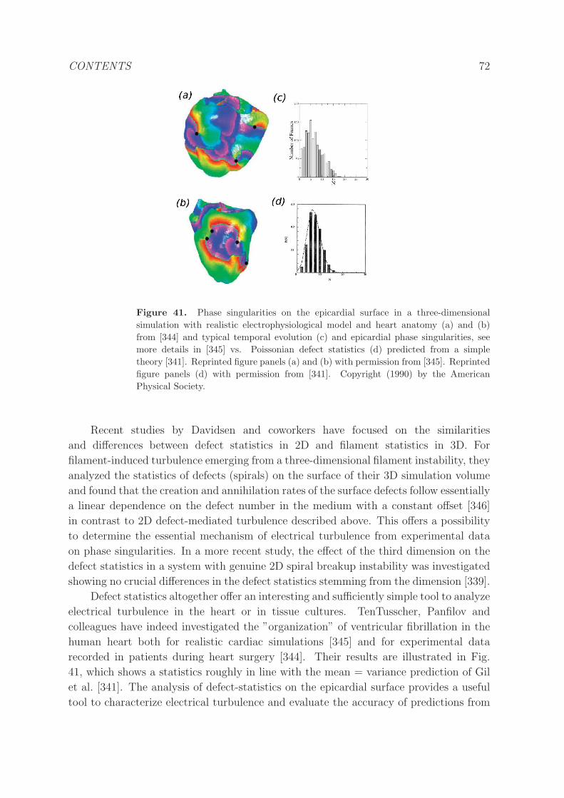
CONTENTS 72
Figure 41. Phase singularities on the epicardial surface in a three-dimensional
simulation with realistic electrophysiological model and heart anatomy (a) and (b)
from [344] and typical temporal evolution (c) and epicardial phase singularities, see
more details in [345] vs. Poissonian defect statistics (d) predicted from a simple
theory [341]. Reprinted figure panels (a) and (b) with permission from [345]. Reprinted
figure panels (d) with permission from [341]. Copyright (1990) by the American
Physical Society.
Recent studies by Davidsen and coworkers have focused on the similarities
and differences between defect statistics in 2D and filament statistics in 3D. For
filament-induced turbulence emerging from a three-dimensional filament instability, they
analyzed the statistics of defects (spirals) on the surface of their 3D simulation volume
and found that the creation and annihilation rates of the surface defects follow essentially
a linear dependence on the defect number in the medium with a constant offset [346]
in contrast to 2D defect-mediated turbulence described above. This offers a possibility
to determine the essential mechanism of electrical turbulence from experimental data
on phase singularities. In a more recent study, the effect of the third dimension on the
defect statistics in a system with genuine 2D spiral breakup instability was investigated
showing no crucial differences in the defect statistics stemming from the dimension [339].
Defect statistics altogether offer an interesting and sufficiently simple tool to analyze
electrical turbulence in the heart or in tissue cultures. TenTusscher, Panfilov and
colleagues have indeed investigated the ”organization” of ventricular fibrillation in the
human heart both for realistic cardiac simulations [345] and for experimental data
recorded in patients during heart surgery [344]. Their results are illustrated in Fig.
41, which shows a statistics roughly in line with the mean = variance prediction of Gil
et al. [341]. The analysis of defect-statistics on the epicardial surface provides a useful
tool to characterize electrical turbulence and evaluate the accuracy of predictions from
CONTENTS 73
computational models with experimental data. A recent application, e.g., compares
defect statistics and other metrics from homogeneous and heterogeneous models [347]
and concludes that the influence of transmural and apicobasical electrophysiological
heterogeneity in electrical turbulence is negligible and may, hence, be discarded in
models. These heterogeneities were included by assigning different electrophysiological
parameters to epicardial, midmyocardial and endocardial cell layers in [347].
CONTENTS 74
8. Theory and methods for spiral and scroll wave instabilities
After the phenomenological description of the different instabilities affecting rotors in
cardiac tissue presented in the previous two sections, we survey in this section theoretical
approaches and numerical methods to study and analyze the instabilities responsible of
complex dynamics in excitable media and cardiac models.
8.1. Kinematic description
In many situations a spiral or scroll wave can be considered as a rigid body, and its
motion reduced to the motion of its tip (for a spiral) or its instantaneous or central
filament (for a scroll). This is particularly valid in the limit of weak excitability,
where this procedure can be performed rigorously using perturbation methods [348–350].
Cardiac tissue, under normal conditions, is highly excitable, so the kinematics equations
in this case have to be considered as a phenomenological description of the motion of
the spiral (or scroll) wave. Still, such a description has helped to understand important
phenomena, as the origin of meander [351], the drift of spirals under an external
field [352–354], or the influence of a periodic forcing [355]. This knowledge has helped
to devise possible methods for defibrillation using low intensity electrical fields [356].
8.1.1. Spiral waves. This phenomenological approach starts by reducing the dynamics
of a spiral wave to the motion of its tip [283,357]. In a Cartesian coordinate frame such
equations are written as
dX
dt= −c sinα− g cosα,
dY
dt= c cosα− g sinα; (67)
where X and Y are the tip coordinates, α its angular variable, and c and g denote,
respectively, the normal and tangential (respective to the spiral curve) tip velocities,
see Fig. 42. These two velocities depend on curvature effects, parametrized by the
instantaneous wavefront curvature at the tip, denoted κ, and are expressed by the
eikonal equation for the normal velocity, and an analogous description for the tangential
velocity:
c = c0 −Dκ, g = g0 − γκ; (68)
in terms of the set of basic kinematic parameters c0 , g0 , D, and γ. In the limit of weak
excitability the curvature correction to the normal velocity can be assumed negligible
(Dκ ≪ c0), so that c reduces to c0.
The particular solution corresponding to a rigid rotating spiral is recovered by
setting α = ω0t and taking g = 0, which gives a critical curvature κc = g0/γ. From the
calculation of the curvature of a spiral wave rotating around an obstacle of radius R0, one
obtains κc = (c0/ξ2DR2
0)1/3 [283], resulting from the limit of Wiener and Rosenblueth
approach of spiral waves [269], with ξ being a numerical constant. Thus, the natural
frequency of the rotating spiral is [283]
ω0 =c0R0
= ξ√
Dc0√
κ3c , (69)
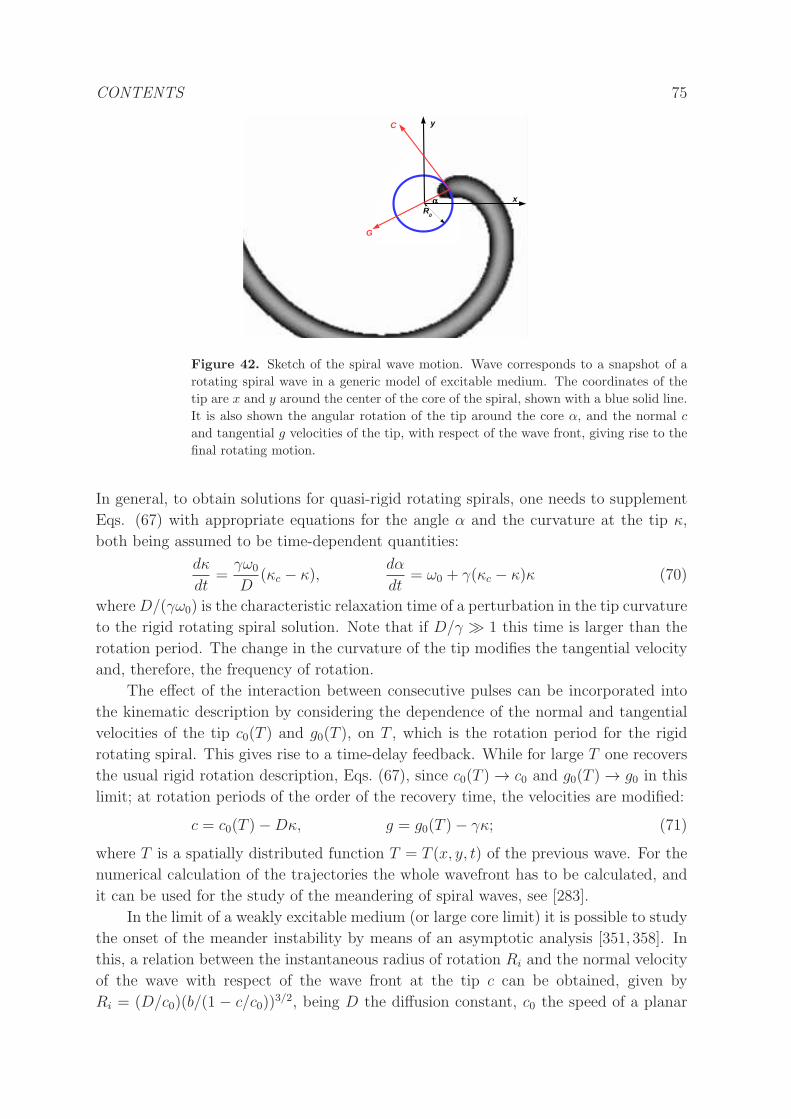
CONTENTS 75
Figure 42. Sketch of the spiral wave motion. Wave corresponds to a snapshot of a
rotating spiral wave in a generic model of excitable medium. The coordinates of the
tip are x and y around the center of the core of the spiral, shown with a blue solid line.
It is also shown the angular rotation of the tip around the core α, and the normal c
and tangential g velocities of the tip, with respect of the wave front, giving rise to the
final rotating motion.
In general, to obtain solutions for quasi-rigid rotating spirals, one needs to supplement
Eqs. (67) with appropriate equations for the angle α and the curvature at the tip κ,
both being assumed to be time-dependent quantities:
dκ
dt=
γω0
D(κc − κ),
dα
dt= ω0 + γ(κc − κ)κ (70)
whereD/(γω0) is the characteristic relaxation time of a perturbation in the tip curvature
to the rigid rotating spiral solution. Note that if D/γ ≫ 1 this time is larger than the
rotation period. The change in the curvature of the tip modifies the tangential velocity
and, therefore, the frequency of rotation.
The effect of the interaction between consecutive pulses can be incorporated into
the kinematic description by considering the dependence of the normal and tangential
velocities of the tip c0(T ) and g0(T ), on T , which is the rotation period for the rigid
rotating spiral. This gives rise to a time-delay feedback. While for large T one recovers
the usual rigid rotation description, Eqs. (67), since c0(T ) → c0 and g0(T ) → g0 in this
limit; at rotation periods of the order of the recovery time, the velocities are modified:
c = c0(T )−Dκ, g = g0(T )− γκ; (71)
where T is a spatially distributed function T = T (x, y, t) of the previous wave. For the
numerical calculation of the trajectories the whole wavefront has to be calculated, and
it can be used for the study of the meandering of spiral waves, see [283].
In the limit of a weakly excitable medium (or large core limit) it is possible to study
the onset of the meander instability by means of an asymptotic analysis [351, 358]. In
this, a relation between the instantaneous radius of rotation Ri and the normal velocity
of the wave with respect of the wave front at the tip c can be obtained, given by
Ri = (D/c0)(b/(1 − c/c0))3/2, being D the diffusion constant, c0 the speed of a planar
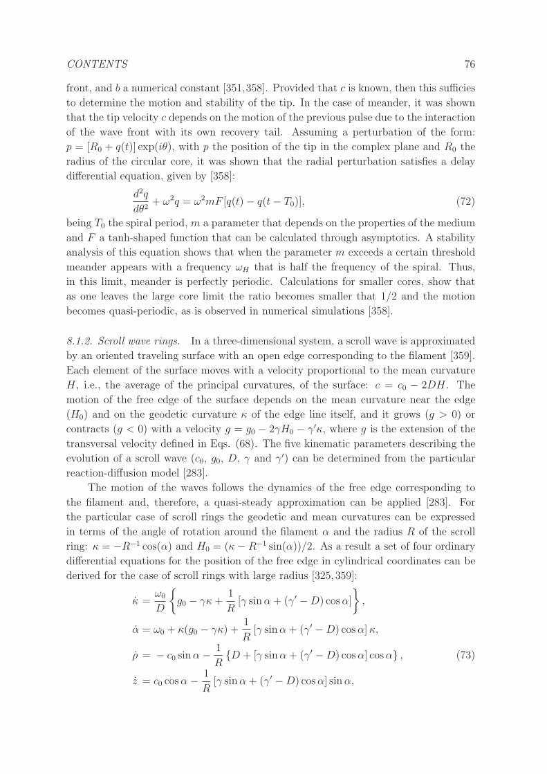
CONTENTS 76
front, and b a numerical constant [351,358]. Provided that c is known, then this sufficies
to determine the motion and stability of the tip. In the case of meander, it was shown
that the tip velocity c depends on the motion of the previous pulse due to the interaction
of the wave front with its own recovery tail. Assuming a perturbation of the form:
p = [R0 + q(t)] exp(iθ), with p the position of the tip in the complex plane and R0 the
radius of the circular core, it was shown that the radial perturbation satisfies a delay
differential equation, given by [358]:
d2q
dθ2+ ω2q = ω2mF [q(t)− q(t− T0)], (72)
being T0 the spiral period, m a parameter that depends on the properties of the medium
and F a tanh-shaped function that can be calculated through asymptotics. A stability
analysis of this equation shows that when the parameter m exceeds a certain threshold
meander appears with a frequency ωH that is half the frequency of the spiral. Thus,
in this limit, meander is perfectly periodic. Calculations for smaller cores, show that
as one leaves the large core limit the ratio becomes smaller that 1/2 and the motion
becomes quasi-periodic, as is observed in numerical simulations [358].
8.1.2. Scroll wave rings. In a three-dimensional system, a scroll wave is approximated
by an oriented traveling surface with an open edge corresponding to the filament [359].
Each element of the surface moves with a velocity proportional to the mean curvature
H, i.e., the average of the principal curvatures, of the surface: c = c0 − 2DH. The
motion of the free edge of the surface depends on the mean curvature near the edge
(H0) and on the geodetic curvature κ of the edge line itself, and it grows (g > 0) or
contracts (g < 0) with a velocity g = g0 − 2γH0 − γ′κ, where g is the extension of the
transversal velocity defined in Eqs. (68). The five kinematic parameters describing the
evolution of a scroll wave (c0, g0, D, γ and γ′) can be determined from the particular
reaction-diffusion model [283].
The motion of the waves follows the dynamics of the free edge corresponding to
the filament and, therefore, a quasi-steady approximation can be applied [283]. For
the particular case of scroll rings the geodetic and mean curvatures can be expressed
in terms of the angle of rotation around the filament α and the radius R of the scroll
ring: κ = −R−1 cos(α) and H0 = (κ− R−1 sin(α))/2. As a result a set of four ordinary
differential equations for the position of the free edge in cylindrical coordinates can be
derived for the case of scroll rings with large radius [325,359]:
κ =ω0
D
g0 − γκ+1
R[γ sinα + (γ′ −D) cosα]
,
α = ω0 + κ(g0 − γκ) +1
R[γ sinα + (γ′ −D) cosα]κ,
ρ = − c0 sinα− 1
RD + [γ sinα + (γ′ −D) cosα] cosα , (73)
z = c0 cosα− 1
R[γ sinα + (γ′ −D) cosα] sinα,
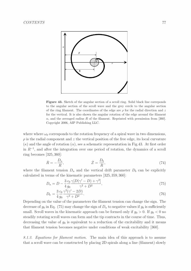
CONTENTS 77
Figure 43. Sketch of the angular section of a scroll ring. Solid black line correponds
to the angular section of the scroll wave and the grey cercle to the angular section
of the ring filament. The coordinates of the edge are ρ for the radial direction and z
for the vertical. It is also shown the angular rotation of the edge around the filament
α, and the averaged radius R of the filament. Reprinted with permission from [360].
Copyright 2006, AIP Publishing LLC.
where where ω0 corresponds to the rotation frequency of a spiral wave in two dimensions,
ρ is the radial component and z the vertical position of the free edge, its local curvature
(κ) and the angle of rotation (α), see a schematic representation in Fig.43. At first order
in R−1, and after the integration over one period of rotation, the dynamics of a scroll
ring becomes [325,360]:
R = −Dn
R, Z =
Db
R, (74)
where the filament tension Dn and the vertical drift parameter Db can be explicitly
calculated in terms of the kinematic parameters [325,359,360]:
Dn = D − 3
4
c0g0
γ[D(γ′ −D) + γ2]
γ2 +D2, (75)
Db =3
4
c0g0
γ2(γ′ − 2D)
γ2 +D2. (76)
Depending on the value of the parameters the filament tension can change the sign. The
decrease of g0 in Eq. (75) may change the sign ofDn to negative values if g0 is sufficiently
small. Scroll waves in the kinematic approach can be formed only if g0 > 0. If g0 < 0 no
steadily rotating scroll waves can form and the tip contracts in the course of time. Thus,
decreasing the value of g0 is equivalent to a reduction of the excitability and it means
that filament tension becomes negative under conditions of weak excitability [360].
8.1.3. Equations for filament motion. The main idea of this approach is to assume
that a scroll wave can be constructed by placing 2D spirals along a line (filament) slowly
CONTENTS 78
varying in space. A periodic rigidly rotating spiral wave satisfies V = V (r, θ − ωt). For
the scroll wave, one can represent the three-dimensional space in the neighborhood of
the filament using the coordinate representation R+ pN+ qB, given by:
dR
ds= T,
dT
ds= κN,
dN
ds= −κT+ τgB,
dB
ds= −τgN, (77)
whereR is the position of the filament, T is the tangent vector, N and B the normal and
binormal unit vectors, s the arclength, κ the curvature and τg the torsion of the filament.
Then, the filament dynamics is represented by coordinates along its length s and in
normal p and binormal q directions yielding to V (s, p, q, t) = V0(r, θ+φ(s, t)−ωt)+V1+...,
(where r and θ are the polar coordinates in the plane p, q) [361].
Starting from the straight, untwisted scroll wave, one can obtain the motion of the
mean filament and the equation for twist, making an expansion in terms of curvature
and torsion, and projecting over the adjoints translational and rotational marginal
eigenmodes (also known as response functions, see [137, 138]). At lowest order this
results in the equations [93, 361]:
∂φ
∂t=
∂N
∂t·B+ b1
(
∂2φ
∂s2− ∂τg
∂s
)
+ a1
(
∂φ
∂s− τg
)2
, (78)
∂R
∂t·N = b2κ, (79)
∂R
∂t·B = c3κ. (80)
where it is imposed the gauge condition ∂tR ·T = 0.
In the case of an untwisted scroll ring, κ = R−1, and the former equations become
simply [93]:
R = −Dn
R, Z =
Db
R, (81)
where R and Z are, respectively, the velocities of the filament in the normal and binormal
directions. The parameters Dn = b2 and Db = c3 can be obtained by calculating the
adjoint eigenfunctions of the linearization around a stable rotating scroll wave [361].
As in the previous section the theory predicts a linear dependence of the radius of the
scroll ring on the curvature. Note, however, that the finding of the adjoint solution is
not trivial and it has to be obtained using numerical methods [138].
The ribbon model (78)-(80) developed by Keener can be extended also to the case
of twist induced instabilities. Defining p(σ, t), the unit vector pointing orthogonally
from the center filament to the line of instantaneous scroll wave tips, the scroll wave
twist can be defined as τ = (p× ∂sp) ·T. Then, a phenomenological extension of Eqs.
(78)-(80) for a twisted scroll wave was developed in [160] (a more rigorous derivation
can be found in [326]), giving
[Rt]⊥ = a1Rss + a2Rs ×Rss + d1τRs ×Rsss − d2τ [Rsss]⊥
− b1[Rssss]⊥ − b2Rs ×Rssss (82)
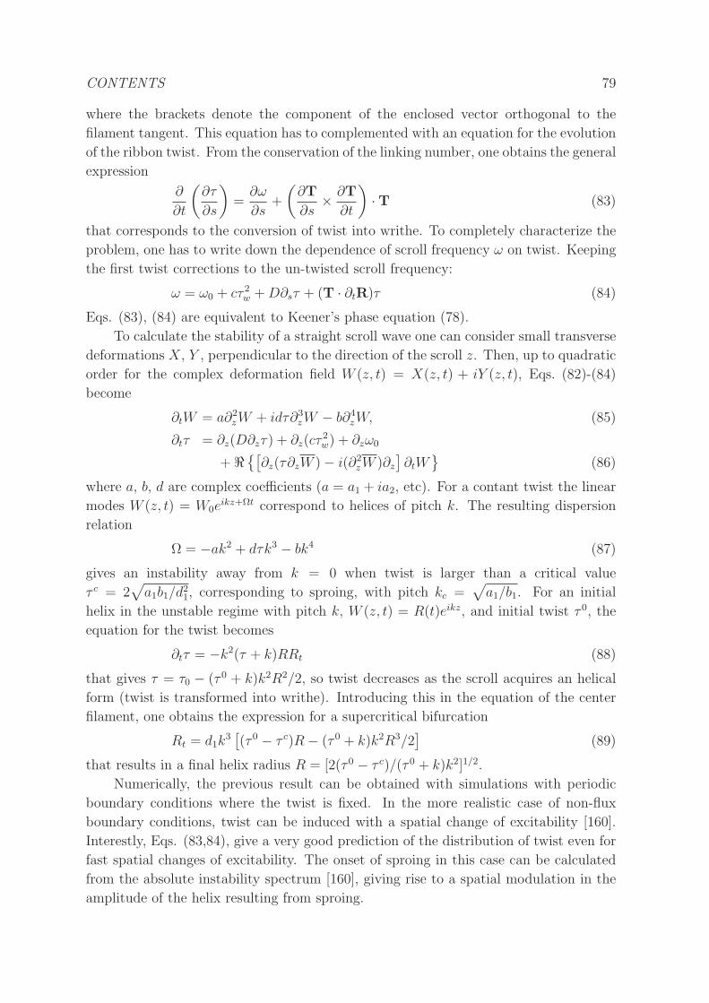
CONTENTS 79
where the brackets denote the component of the enclosed vector orthogonal to the
filament tangent. This equation has to complemented with an equation for the evolution
of the ribbon twist. From the conservation of the linking number, one obtains the general
expression
∂
∂t
(
∂τ
∂s
)
=∂ω
∂s+
(
∂T
∂s× ∂T
∂t
)
·T (83)
that corresponds to the conversion of twist into writhe. To completely characterize the
problem, one has to write down the dependence of scroll frequency ω on twist. Keeping
the first twist corrections to the un-twisted scroll frequency:
ω = ω0 + cτ 2w +D∂sτ + (T · ∂tR)τ (84)
Eqs. (83), (84) are equivalent to Keener’s phase equation (78).
To calculate the stability of a straight scroll wave one can consider small transverse
deformations X, Y , perpendicular to the direction of the scroll z. Then, up to quadratic
order for the complex deformation field W (z, t) = X(z, t) + iY (z, t), Eqs. (82)-(84)
become
∂tW = a∂2zW + idτ∂3
zW − b∂4zW, (85)
∂tτ = ∂z(D∂zτ) + ∂z(cτ2w) + ∂zω0
+ ℜ[
∂z(τ∂zW )− i(∂2zW )∂z
]
∂tW
(86)
where a, b, d are complex coefficients (a = a1 + ia2, etc). For a contant twist the linear
modes W (z, t) = W0eikz+Ωt correspond to helices of pitch k. The resulting dispersion
relation
Ω = −ak2 + dτk3 − bk4 (87)
gives an instability away from k = 0 when twist is larger than a critical value
τ c = 2√
a1b1/d21, corresponding to sproing, with pitch kc =√
a1/b1. For an initial
helix in the unstable regime with pitch k, W (z, t) = R(t)eikz, and initial twist τ 0, the
equation for the twist becomes
∂tτ = −k2(τ + k)RRt (88)
that gives τ = τ0 − (τ 0 + k)k2R2/2, so twist decreases as the scroll acquires an helical
form (twist is transformed into writhe). Introducing this in the equation of the center
filament, one obtains the expression for a supercritical bifurcation
Rt = d1k3[
(τ 0 − τ c)R− (τ 0 + k)k2R3/2]
(89)
that results in a final helix radius R = [2(τ 0 − τ c)/(τ 0 + k)k2]1/2.
Numerically, the previous result can be obtained with simulations with periodic
boundary conditions where the twist is fixed. In the more realistic case of non-flux
boundary conditions, twist can be induced with a spatial change of excitability [160].
Interestly, Eqs. (83,84), give a very good prediction of the distribution of twist even for
fast spatial changes of excitability. The onset of sproing in this case can be calculated
from the absolute instability spectrum [160], giving rise to a spatial modulation in the
amplitude of the helix resulting from sproing.
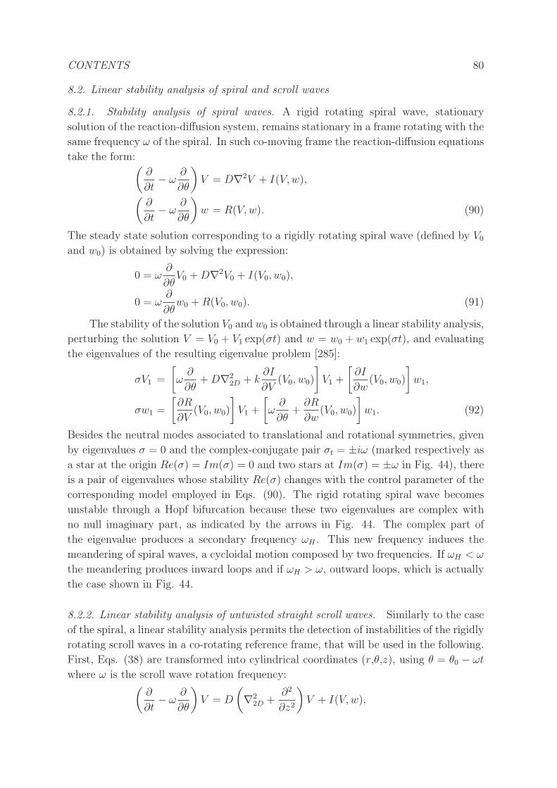
CONTENTS 80
8.2. Linear stability analysis of spiral and scroll waves
8.2.1. Stability analysis of spiral waves. A rigid rotating spiral wave, stationary
solution of the reaction-diffusion system, remains stationary in a frame rotating with the
same frequency ω of the spiral. In such co-moving frame the reaction-diffusion equations
take the form:(
∂
∂t− ω
∂
∂θ
)
V = D∇2V + I(V,w),
(
∂
∂t− ω
∂
∂θ
)
w = R(V,w). (90)
The steady state solution corresponding to a rigidly rotating spiral wave (defined by V0
and w0) is obtained by solving the expression:
0 = ω∂
∂θV0 +D∇2V0 + I(V0, w0),
0 = ω∂
∂θw0 +R(V0, w0). (91)
The stability of the solution V0 and w0 is obtained through a linear stability analysis,
perturbing the solution V = V0 + V1 exp(σt) and w = w0 + w1 exp(σt), and evaluating
the eigenvalues of the resulting eigenvalue problem [285]:
σV1 =
[
ω∂
∂θ+D∇2
2D + k∂I
∂V(V0, w0)
]
V1 +
[
∂I
∂w(V0, w0)
]
w1,
σw1 =
[
∂R
∂V(V0, w0)
]
V1 +
[
ω∂
∂θ+
∂R
∂w(V0, w0)
]
w1. (92)
Besides the neutral modes associated to translational and rotational symmetries, given
by eigenvalues σ = 0 and the complex-conjugate pair σt = ±iω (marked respectively as
a star at the origin Re(σ) = Im(σ) = 0 and two stars at Im(σ) = ±ω in Fig. 44), there
is a pair of eigenvalues whose stability Re(σ) changes with the control parameter of the
corresponding model employed in Eqs. (90). The rigid rotating spiral wave becomes
unstable through a Hopf bifurcation because these two eigenvalues are complex with
no null imaginary part, as indicated by the arrows in Fig. 44. The complex part of
the eigenvalue produces a secondary frequency ωH . This new frequency induces the
meandering of spiral waves, a cycloidal motion composed by two frequencies. If ωH < ω
the meandering produces inward loops and if ωH > ω, outward loops, which is actually
the case shown in Fig. 44.
8.2.2. Linear stability analysis of untwisted straight scroll waves. Similarly to the case
of the spiral, a linear stability analysis permits the detection of instabilities of the rigidly
rotating scroll waves in a co-rotating reference frame, that will be used in the following.
First, Eqs. (38) are transformed into cylindrical coordinates (r,θ,z), using θ = θ0 − ωt
where ω is the scroll wave rotation frequency:(
∂
∂t− ω
∂
∂θ
)
V = D
(
∇22D +
∂2
∂z2
)
V + I(V,w),
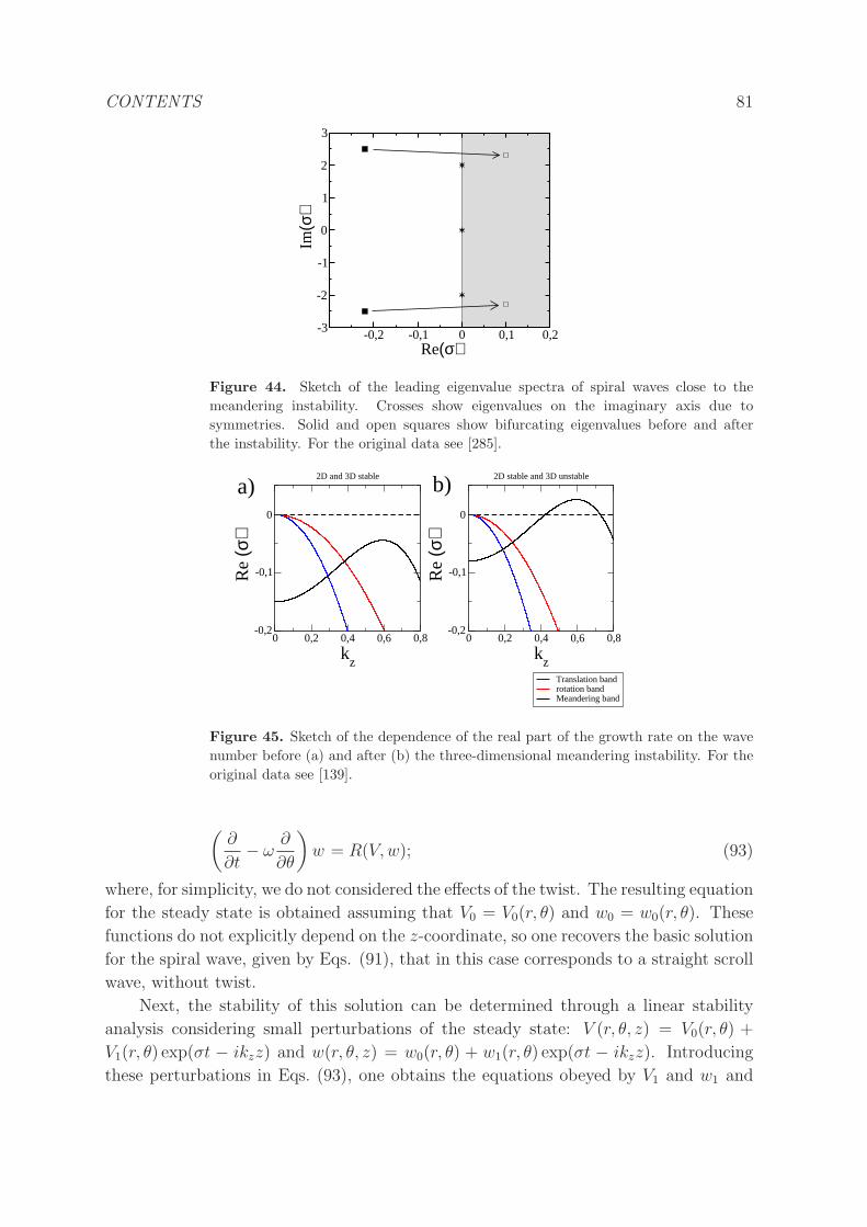
CONTENTS 81
-0,2 -0,1 0 0,1 0,2Re(σ)
-3
-2
-1
0
1
2
3
Im(σ
)
Figure 44. Sketch of the leading eigenvalue spectra of spiral waves close to the
meandering instability. Crosses show eigenvalues on the imaginary axis due to
symmetries. Solid and open squares show bifurcating eigenvalues before and after
the instability. For the original data see [285].
0 0,2 0,4 0,6 0,8
kz
-0,2
-0,1
0
Re
(σ)
Translation bandrotation bandMeandering band
2D and 3D stable
0 0,2 0,4 0,6 0,8
kz
-0,2
-0,1
0
Re
(σ)
2D stable and 3D unstable
a) b)
Figure 45. Sketch of the dependence of the real part of the growth rate on the wave
number before (a) and after (b) the three-dimensional meandering instability. For the
original data see [139].
(
∂
∂t− ω
∂
∂θ
)
w = R(V,w); (93)
where, for simplicity, we do not considered the effects of the twist. The resulting equation
for the steady state is obtained assuming that V0 = V0(r, θ) and w0 = w0(r, θ). These
functions do not explicitly depend on the z-coordinate, so one recovers the basic solution
for the spiral wave, given by Eqs. (91), that in this case corresponds to a straight scroll
wave, without twist.
Next, the stability of this solution can be determined through a linear stability
analysis considering small perturbations of the steady state: V (r, θ, z) = V0(r, θ) +
V1(r, θ) exp(σt − ikzz) and w(r, θ, z) = w0(r, θ) + w1(r, θ) exp(σt − ikzz). Introducing
these perturbations in Eqs. (93), one obtains the equations obeyed by V1 and w1 and
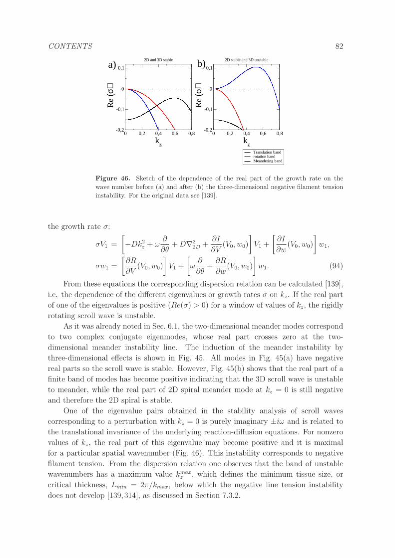
CONTENTS 82
0 0,2 0,4 0,6 0,8
kz
-0,2
-0,1
0
0,1
Re
(σ)
Translation bandrotation bandMeandering band
2D and 3D stable
0 0,2 0,4 0,6 0,8
kz
-0,2
-0,1
0
0,1
Re
(σ)
2D stable and 3D unstable
a) b)
Figure 46. Sketch of the dependence of the real part of the growth rate on the
wave number before (a) and after (b) the three-dimensional negative filament tension
instability. For the original data see [139].
the growth rate σ:
σV1 =
[
−Dk2z + ω
∂
∂θ+D∇2
2D +∂I
∂V(V0, w0)
]
V1 +
[
∂I
∂w(V0, w0)
]
w1,
σw1 =
[
∂R
∂V(V0, w0)
]
V1 +
[
ω∂
∂θ+
∂R
∂w(V0, w0)
]
w1. (94)
From these equations the corresponding dispersion relation can be calculated [139],
i.e. the dependence of the different eigenvalues or growth rates σ on kz. If the real part
of one of the eigenvalues is positive (Re(σ) > 0) for a window of values of kz, the rigidly
rotating scroll wave is unstable.
As it was already noted in Sec. 6.1, the two-dimensional meander modes correspond
to two complex conjugate eigenmodes, whose real part crosses zero at the two-
dimensional meander instability line. The induction of the meander instability by
three-dimensional effects is shown in Fig. 45. All modes in Fig. 45(a) have negative
real parts so the scroll wave is stable. However, Fig. 45(b) shows that the real part of a
finite band of modes has become positive indicating that the 3D scroll wave is unstable
to meander, while the real part of 2D spiral meander mode at kz = 0 is still negative
and therefore the 2D spiral is stable.
One of the eigenvalue pairs obtained in the stability analysis of scroll waves
corresponding to a perturbation with kz = 0 is purely imaginary ±iω and is related to
the translational invariance of the underlying reaction-diffusion equations. For nonzero
values of kz, the real part of this eigenvalue may become positive and it is maximal
for a particular spatial wavenumber (Fig. 46). This instability corresponds to negative
filament tension. From the dispersion relation one observes that the band of unstable
wavenumbers has a maximum value kmaxz , which defines the minimum tissue size, or
critical thickness, Lmin = 2π/kmax, below which the negative line tension instability
does not develop [139,314], as discussed in Section 7.3.2.
CONTENTS 83
8.2.3. Linear stability analysis of twisted straight scroll waves. In this case we employ
Eqs. (93) in cylindrical coordinates (r,θ,z), where the amount of twist τ in the scroll
wave is explicitly considered using θ = θ0 − ωt− τz:(
∂
∂t− ω
∂
∂θ
)
V = D
(
∇22D +
∂2
∂z2− 2τ
∂2
∂θ∂z+ τ 2
∂2
∂θ2
)
V + I(V,w),
(
∂
∂t− ω
∂
∂θ
)
w = R(V,w); (95)
see for more details [314]. The resulting equation for the steady state is obtained
assuming that V0 = V0(r, θ) and w0 = w0(r, θ). As in the previous case, the stability
of this solution can be determined through a linear stability analysis introducing small
perturbations of the steady state: V (r, θ, z) = V0(r, θ) + V1(r, θ) exp(σt − ikzz) and
w(r, θ, z) = w0(r, θ) + w1(r, θ) exp(σt− ikzz) into Eqs. (95):
σV1 =
[
−Dk2z + ω
∂
∂θ+Dτ 2
∂2
∂θ2+ 2Diτkz
∂
∂θ+D∇2
2D +∂I
∂V(V0, w0)
]
V1
+
[
∂I
∂w(V0, w0)
]
w1,
σw1 =
[
∂R
∂V(V0, w0)
]
V1 +
[
ω∂
∂θ+
∂R
∂w(V0, w0)
]
w1. (96)
For nonzero twist (τ 6= 0 ) the dispersion relations obtained from Eq. (96) are not
symmetric with respect kz and therefore σ does not depend only in k2z but also on odd
powers of kz.
8.3. Normal form analysis of the meander transition
8.3.1. Spiral waves. A simple phenomenological analysis of the transition to meander
was developed by Barkley [286] and further formalized by Sandstede & Scheel [287].
In this, a normal form is derived for the bifurcation to meander, assuming that it
occurs as a supercritical Hopf bifurcation, and taking into account Euclidean symmetry
(rotation plus translations in the plane). Then, at the onset of the instability there are
five marginal modes, corresponding to translational and rotational symmetry, and the
modes emerging from the Hopf bifurcation. With this, the model reads:
φ = ω (97)
p = eiφ(iωR0 − z) (98)
z = (λH − |z|2)z (99)
where φ is the phase of the circular motion of the spiral tip, and the complex functions
p = x+ iy and z = ρeiα are the position of the tip and the (complex) amplitude of the
Hopf modes. Besides, the Hopf and translational eigenvalues are given by λH = µ+ iωH
and λT = iω, respectively (note that the equations are written in the original, not in
the comoving, frame). When µ < 0 the Hopf modes decay to zero, and the solution is
CONTENTS 84
a rigidly rotating spiral p(t) = R0eiωt. When µ > 0, then, taking z = ρeiα, for the Hopf
mode one obtains:
ρ = (µ− ρ2)ρ, α = ωH , (100)
which, assuming that the amplitude decays fast to its steady state value, gives ρ =√µ,
α = α0 + ωHt. Then, the motion of the tip of the spiral is given by:
p = iωR0eiωt −√
µe−iα0+i(ω−ωH)t. (101)
When the frequency of the Hopf modes is the same as the original frequency of the
spiral ωH = ω, this equation results in a linear drift of the tip:
p(t) = R0eiωt −√
µte−iα0 , (102)
If the frequencies are different, ωH 6= ω then, the solution reads:
p(t) = R0eiωt +
iõ
ω − ωH
e−iα0+i(ω−ωH)t, (103)
that results in outward or inward petals depending on the relative values of ω and ωH .
These type of normal forms can also be used, for instance, to study the resonant
drift of the spirals under the effect of a periodic forcing [362].
8.3.2. Scroll waves. The normal form of a spiral wave under meandering (97)-(99) has
to be modified in order to take into account the effects of a small curvature of slightly
curved filaments of a 3D scroll wave [315].
dφ
dt= ω,
∂p
∂t= eiφ(iωR0 − z) + β
∂2p
∂z2,
∂z
∂t= (µ− iωH − |z|2)z + γe−iφ∂
2p
∂z2. (104)
Using a perturbation of the form p = R0eiωt+p1e
iφeσt+ikzz and z = z1eσt+ikzz, where
R0eiωt is the steady scroll wave solution, one obtains the eigenvalues corresponding to
the meander and translation bands. The eigenvalue for meandering becomes:
σH = µ− iωH −[
γ
µ+ i(ω − ωH)
]
k2z ; (105)
so σH depends on kz, and therefore the bifurcation line of 3D meander may be different
than 2D meandering. The eigenvalue corresponding to the translation band is:
σt = −iω +
[
β +γ
µ+ i(ω − ωH)
]
k2z ; (106)
which indicates that the real value of σ depends on kz, and for large enough values of
γ the eigenvalue may become positive. The curvature at the origin of the translation
band is the same as the drift velocity of a spiral in the presence of a electric field. It
is also equal to the opposite of the curvature of the meander band shifted by a factor
β [315]. The specific form of the coefficients γ and β can be found in [315].
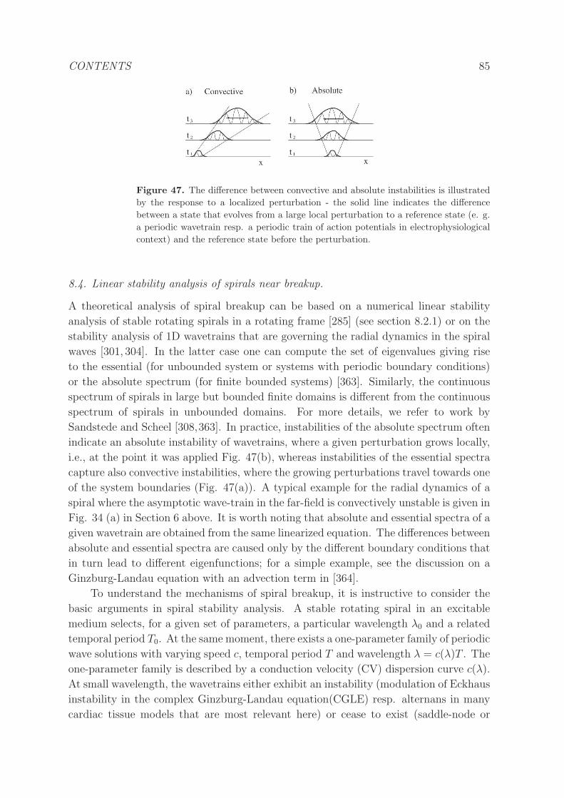
CONTENTS 85
Figure 47. The difference between convective and absolute instabilities is illustrated
by the response to a localized perturbation - the solid line indicates the difference
between a state that evolves from a large local perturbation to a reference state (e. g.
a periodic wavetrain resp. a periodic train of action potentials in electrophysiological
context) and the reference state before the perturbation.
8.4. Linear stability analysis of spirals near breakup.
A theoretical analysis of spiral breakup can be based on a numerical linear stability
analysis of stable rotating spirals in a rotating frame [285] (see section 8.2.1) or on the
stability analysis of 1D wavetrains that are governing the radial dynamics in the spiral
waves [301, 304]. In the latter case one can compute the set of eigenvalues giving rise
to the essential (for unbounded system or systems with periodic boundary conditions)
or the absolute spectrum (for finite bounded systems) [363]. Similarly, the continuous
spectrum of spirals in large but bounded finite domains is different from the continuous
spectrum of spirals in unbounded domains. For more details, we refer to work by
Sandstede and Scheel [308,363]. In practice, instabilities of the absolute spectrum often
indicate an absolute instability of wavetrains, where a given perturbation grows locally,
i.e., at the point it was applied Fig. 47(b), whereas instabilities of the essential spectra
capture also convective instabilities, where the growing perturbations travel towards one
of the system boundaries (Fig. 47(a)). A typical example for the radial dynamics of a
spiral where the asymptotic wave-train in the far-field is convectively unstable is given in
Fig. 34 (a) in Section 6 above. It is worth noting that absolute and essential spectra of a
given wavetrain are obtained from the same linearized equation. The differences between
absolute and essential spectra are caused only by the different boundary conditions that
in turn lead to different eigenfunctions; for a simple example, see the discussion on a
Ginzburg-Landau equation with an advection term in [364].
To understand the mechanisms of spiral breakup, it is instructive to consider the
basic arguments in spiral stability analysis. A stable rotating spiral in an excitable
medium selects, for a given set of parameters, a particular wavelength λ0 and a related
temporal period T0. At the same moment, there exists a one-parameter family of periodic
wave solutions with varying speed c, temporal period T and wavelength λ = c(λ)T . The
one-parameter family is described by a conduction velocity (CV) dispersion curve c(λ).
At small wavelength, the wavetrains either exhibit an instability (modulation of Eckhaus
instability in the complex Ginzburg-Landau equation(CGLE) resp. alternans in many
cardiac tissue models that are most relevant here) or cease to exist (saddle-node or
CONTENTS 86
drift pitchfork bifurcations in FitzHugh-Nagumo systems [365, 366]). If the wavelength
selected by the spiral is smaller than this minimum value, it will be unstable. These
minimum stable wavelengths and periods shall be called λmin, respectively Tmin, in the
following. Only in a few cases (e.g. for the CGLE describing oscillatory media [367],
or the Rinzel-Keller model of an excitable medium [368]), it is possible to compute
the instabilities or bifurcations analytically. In other cases, simpler kinematic theories
(see above section on alternans) or approximations by singular perturbation theory
(excitable media) may yield useful information on the nature of this instability. For
the models employed in cardiac dynamics, none of these methods are sufficient to yield
an understanding of the instability at λmin. This calls again for alternative methods,
namely numerical stability analysis of traveling waves, introduced above in Section 5.2.3.
8.4.1. Linear stability analysis of periodic traveling waves. One has to numerically
compute the 1D wave solutions and their linear stability along the dispersion curve.
Continuation software as AUTO can be used to obtain the spatial profiles U0(z)
of periodic waves as stationary solutions in a co-moving frame z = r − ct [369].
Consequently, one needs to compute periodic orbits that correspond to a single
wavelength with periodic boundary conditions. The evolution of small perturbations of
a spatially periodic travelling wave U0(z) in the reaction diffusion equations is described
by Wjn(z)eωjnt, where Wjn(z) and ωjn are eigenvectors and eigenvalues of the linearized
equations. For continuum models such as the reaction-diffusion equations used in
electrophysiology, there are infinitely many eigenvalues and eigenfunctions as the system
length L → ∞. Consequently, the ωjn are located on continuous curves in the complex
plane. A wavetrain solution is stable when all eigenvalues ωjn have non-positive real
parts. If the wavelength λ is used as a bifurcation parameter, the described method
yields accurate information on the minimum stable wavelength λmin for a given model
and parameter set, where the eigenvalue spectra and the eigenfunctions describe the
dynamics of perturbations to the wavetrains.
If one considers periodic travelling waves with constant shape U0(z) and constant
speed c in 1D, a few facts on the eigenvalues and the eigenfunctions are known a priori. If
the cardiac model is spatially homogeneous, any translation of a given periodic solution
is also a valid solution with identical stability properties. This translational symmetry
of the wavetrains is reflected by an eigenvector W00 = dU0/dz with zero eigenvalue
ω00 = 0 (Goldstone mode). Symmetry arguments require the eigenfunctions of the
periodic operator, obtained by linearization around a wavetrain with wavelength λ, to
be Bloch functions Wjn(z) = ei(2πn/L)zφjn(z) = eikzφjn(z) with φjn(z) = φjn(z + λ) and
n = 0, . . . , N −1 [370]. The above Bloch form can be used in an ansatz that reduces the
stability problem for the infinite domain to a stability problem in a domain of length λ
with the wavenumber k = 2πn/L as an additional parameter. If one assumes a purely
imaginary exponent ikz in the prefactor of the Bloch eigenfunctions, one obtains the
so-called essential spectrum. To assess the stability of spirals in finite domains, one
needs, however, to compute also the absolute spectrum. This can be done by employing
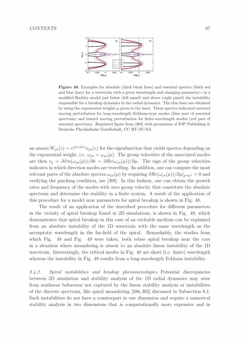
CONTENTS 87
Figure 48. Examples for absolute (thick black lines) and essential spectra (thick red
and blue lines) for a wavetrain with a given wavelength and changing parameter ǫ in a
modified Barkley model just below (left panel) and above (right panel) the instability
responsible for a breakup dynamics in the radial dynamics. The thin lines are obtained
by using the exponential weights µ given in the inset. These spectra indicated outward
moving perturbation for long-wavelength Eckhaus-type modes (blue part of essential
spectrum) and inward moving perturbation for finite-wavelength modes (red part of
essential spectrum). Reprinted figure from [304] with permission of IOP Publishing &
Deutsche Physikalische Gesellschaft, CC BY-NC-SA.
an ansatz Wjn(z) = e(µ+ik)zφjn(z) for the eigenfunction that yields spectra depending on
the exponential weight, i.e. ωjn = ωjn(µ). The group velocities of the associated modes
are then vg = ∂Im(ωjn(µ))/∂k = ∂Re(ωjn(µ))/∂µ. The sign of the group velocities
indicates in which direction modes are travelling. In addition, one can compute the most
relevant parts of the absolute spectra ωjn(µ) by requiring ∂Re(ωjn(µ))/∂µ|µ=µ∗ = 0 and
verifying the pinching condition, see [308]. In this fashion, one can obtain the growth
rates and frequency of the modes with zero group velocity that constitute the absolute
spectrum and determine the stability in a finite system. A result of the application of
this procedure for a model near parameters for spiral breakup is shown in Fig. 48.
The result of an application of the described procedure for different parameters
in the vicinity of spiral breakup found in 2D simulations, is shown in Fig. 49, which
demonstrates that spiral breakup in this case of an excitable medium can be explained
from an absolute instability of the 1D wavetrain with the same wavelength as the
asymptotic wavelength in the far-field of the spiral. Remarkably, the studies from
which Fig. 48 and Fig. 49 were taken, both relate spiral breakup near the core
in a situation where meandering is absent to an absolute linear instability of the 1D
wavetrain. Interestingly, the critical modes in Fig. 48 are short (i.e. finite) wavelength
whereas the instability in Fig. 49 results from a long-wavelength Eckhaus instability.
8.4.2. Spiral instabilities and breakup phenomenologies. Potential discrepancies
between 2D simulation and stability analysis of the 1D radial dynamics may arise
from nonlinear behaviour not captured by the linear stability analysis or instabilities
of the discrete spectrum, like spiral meandering [286, 302] discussed in Subsection 6.1.
Such instabilities do not have a counterpart in one dimension and require a numerical
stability analysis in two dimensions that is computationally more expensive and in
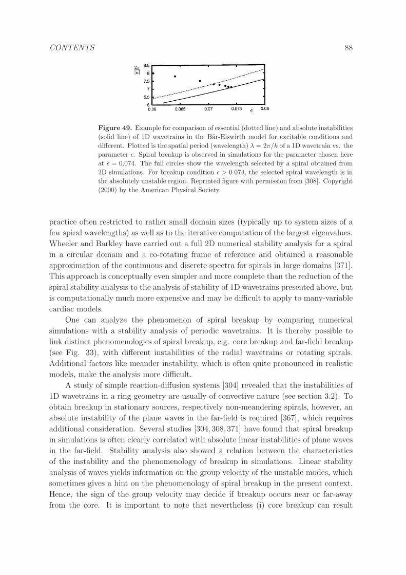
CONTENTS 88
Figure 49. Example for comparison of essential (dotted line) and absolute instabilities
(solid line) of 1D wavetrains in the Bar-Eiswirth model for excitable conditions and
different. Plotted is the spatial period (wavelength) λ = 2π/k of a 1D wavetrain vs. the
parameter ǫ. Spiral breakup is observed in simulations for the parameter chosen here
at ǫ = 0.074. The full circles show the wavelength selected by a spiral obtained from
2D simulations. For breakup condition ǫ > 0.074, the selected spiral wavelength is in
the absolutely unstable region. Reprinted figure with permission from [308]. Copyright
(2000) by the American Physical Society.
practice often restricted to rather small domain sizes (typically up to system sizes of a
few spiral wavelengths) as well as to the iterative computation of the largest eigenvalues.
Wheeler and Barkley have carried out a full 2D numerical stability analysis for a spiral
in a circular domain and a co-rotating frame of reference and obtained a reasonable
approximation of the continuous and discrete spectra for spirals in large domains [371].
This approach is conceptually even simpler and more complete than the reduction of the
spiral stability analysis to the analysis of stability of 1D wavetrains presented above, but
is computationally much more expensive and may be difficult to apply to many-variable
cardiac models.
One can analyze the phenomenon of spiral breakup by comparing numerical
simulations with a stability analysis of periodic wavetrains. It is thereby possible to
link distinct phenomenologies of spiral breakup, e.g. core breakup and far-field breakup
(see Fig. 33), with different instabilities of the radial wavetrains or rotating spirals.
Additional factors like meander instability, which is often quite pronounced in realistic
models, make the analysis more difficult.
A study of simple reaction-diffusion systems [304] revealed that the instabilities of
1D wavetrains in a ring geometry are usually of convective nature (see section 3.2). To
obtain breakup in stationary sources, respectively non-meandering spirals, however, an
absolute instability of the plane waves in the far-field is required [367], which requires
additional consideration. Several studies [304, 308, 371] have found that spiral breakup
in simulations is often clearly correlated with absolute linear instabilities of plane waves
in the far-field. Stability analysis also showed a relation between the characteristics
of the instability and the phenomenology of breakup in simulations. Linear stability
analysis of waves yields information on the group velocity of the unstable modes, which
sometimes gives a hint on the phenomenology of spiral breakup in the present context.
Hence, the sign of the group velocity may decide if breakup occurs near or far-away
from the core. It is important to note that nevertheless (i) core breakup can result
CONTENTS 89
from different types of instability and that (ii) the same instability scenario may lead
to phenomenologically different appearances. In other words, the form of the linearly
unstable modes is not sufficient to determine the full nonlinear spatiotemporal dynamics.
Moreover, a particular phenomenology found in simulations does not necessary allow
a conclusion on the specific nature of the linear instability presumably behind it. To
obtain the full information, direct simulations and an independent linear stability are
hence necessary. In many cardiac models, core breakup is presumably caused by an
alternans instability of the wavetrains emitted from the spiral core [225,279,292,372].
The influence of meandering and the resulting Doppler effect in core breakup
has been verified in simulations [91] and experiments with the Belousov-Zhabotinsky
reaction [290]. Far-field breakup of (presumably) meandering spirals with a non-
decaying modulation of the wavetrain in the far-field (’superspirals’ [287,373]) has been
studied in the same reaction [309,310]. Here, an interpretation of the breakup in terms
of the non-linear consequences of the Eckhaus instability has been given [303]. Most
of results for the stability analysis of spirals near the onset of breakup were obtained
for simple reaction-diffusion systems. The analysis and numerical procedures described
here may be applied to simple cardiac models like the Aliev-Panfilov model [79] or the
variant of the Noble model studied by Karma [84]. This should enable researchers to
elucidate the mechanisms behind the rich phenomenology of spiral breakup found in
cardiac models [40]. Finally, the hypothesis that alternans is the crucial instability
behind spiral breakup maybe tested and possible alternatives may be uncovered.
CONTENTS 90
9. Discussion and outlook
Cardiac arrhythmias are potential triggers of sudden cardiac death, which is the main
cause of death in the developed world [374], and a plethora of other health risks.
The transition between healthy and pathological tissue dynamics may have different
causes, e.g., myocardial ischemia, infarction or genetic predisposition. Similarly, the
dynamical mechanisms governing such a transition are not unique and often not well
understood. As a result mathematical modeling of action potential propagation in the
heart has become a major research topic during the last two decades. Realistic models
of cardiac tissue include hundred of dynamical coupled equations evolving in complex
and asymmetrical geometries.
A huge growth of computational capabilities and numerical algorithms in the last
years has enabled direct numerical simulations, employing these models, to reproduce
the main properties of cardiac arrhythmia and the associated dynamical transitions.
However, mechanistic interpretations of the transition are often difficult and missing for
realistic cardiac models. Therefore, we have reviewed here often findings in simplified
models of cardiac tissue to analyze the different mechanisms of instabilities in cardiac
dynamics and provided simplified theoretical descriptions.
Altogether, cardiac modeling has emerged as one of the prime application areas of
theories and methods of nonlinear physics originally developed for pattern formation in
extended nonequilibrium media. Rotors are believed to be formed in reentry and are
crucial for the appearance of arrhythmias like ventricular tachycardia (VT) as well as
atrial and ventricular fibrillation (AF,VF). Therefore, a substantial part of this review
is focused on the dynamics and potential instabilities of such structures.
We have reviewed the related advances in theory, the different numerical and
analytical methods that have been developed in recent years and their application to
cardiac dynamics. According to Jalife [4] in particular rotors are crucial:“AF and
VT/VF are by far the most significant cardiac arrhythmias faced by the physician.
Owing to their highly complex electrocardiographic appearance, both AF and VF are
commonly thought of as being the result of exceptionally complex and disorganized cardiac
activation, in which electrical waves propagate through the atria or ventricles chaotically
and unpredictably. In fact, during fibrillation the electrical activation sequence is
profoundly abnormal; electrical wave fronts do not follow the usual paths. The atrial or
ventricular rates accelerate to the extreme and electrical waves assume a complex vortex-
like behavior that looks a lot like eddy formation and turbulence in water. Recent evidence
strongly suggesting that rotors are critical in sustaining both atrial and ventricular
fibrillation (AF, VF) in the human heart, which may have critical implications for
treatment with radio-frequency ablation.” This passage illustrates the fruitful exchange
between the nonlinear physics and the cardiology communities that has been the main
theme of this review article.
What has been achieved is a detailed understanding of a few central phenomena.
Often this has been done initially for largely simplified cardiac model equations. The
CONTENTS 91
findings and the associated methods described here can, however, also be applied to more
realistic electrophysiological models and may in the future help the analysis of newly
developed computational models. The starting point for a nonlinear dynamics treatment
of cardiac propagation is a periodic sequence of action potentials corresponding to (a
somewhat idealized) normal sine rhythm. This rhythm is parametrized by its frequency
and the wavelength of subsequent action potentials and corresponding velocities.
A key instability that already occurs in the local dynamics of paced cardiac
cells is cardiac alternans (Section 5), which is a period doubling of the oscillation in
the membrane potential of a single cardiac cell occurring at sufficiently large pacing
frequency. In a single cell the onset of alternans can be predicted from the action
potential duration (APD) restitution curve that describes the dependency of the time
a specific AP lasts on the diastolic interval The map approach, amplitude equations as
well as numerical linear analysis of APD trains allow accurate predictions for the onset
of alternans. Many of these theories are not rigorous and therefore need comparison
with direct numerical simulations. In tissue, alternans may occur in two different
forms, namely discordant and concordant alternans. Discordant alternans is particularly
relevant and may lead to further complications like APD block and formation of rotors.
The mechanism of its occurrence has been worked out nicely in the framework of
amplitude equations.
The dynamics of rotors invokes many complicated phenomena. Rotors in cardiac
tissues behave usually in a complicated manner. This is a result of various dynamical
instabilities of the spirals rigid rotation (Section 6). These may act upon the core region
near the tip or in the far-field of periodic waves of a spiral or affect both aspects. Most
electrophysiological models display strong meandering, a well understood phenomenon
stemming from an oscillatory instability of the tip motion. Instabilities in the far-field
lead typically to the destruction of coherent spiral patterns and to formation of new
rotors by spiral breakup.
Scroll waves are subject to many new instabilities like negative filament line tension
and sproing that were described in Section 7, that also contains a discussion on the
state-of-the art characterization of electrical turbulence. Finally, Section 8 deals with
approaches to analyze the instabilities behind the complex dynamical phenomenologies
found in simulations of cardiac dynamics and corresponding experiments. A main
result is that changes in behavior of rotors are often associated with linear instabilities.
Numerical stability analysis can then give an accurate determination of critical
parameters, nature of instabilities and bifurcation and their spatiotemporal signatures.
A popular view cited in many talks and publications, see e.g. [15, 40] is that the
mechanism for ventricular fibrillation may develop from a rotor that occurs from a
perturbation of the regular sine rhythm. The rotor is the center of a spiral wave
that typically has a much higher frequency than the sine rhythm in cardiac tissue
and therefore occurs as tachycardia. If this spiral is unstable a more irregular pattern
appears that bears the signature of fibrillation. Alternative explanations for the irregular
dynamics observed in fibrillation have featured a single drifting or wildly moving
CONTENTS 92
(meandering) rotor or electrical turbulence forming at some distance from a spiral
(mother rotor) center. All these scenarios can be traced back to the different instabilities
described in this review and are, in principle, possible in perfectly homogeneous
tissue. Since healthy tissue usually is not subject to the cascade of events leading
to fibrillatory activity, functional reentry may occur as a result of pathological changes
in the electrophysiological properties of the myocytes.
While this review mostly has dealt with cardiac propagation in homogeneous and
isotropic media, the true heart has a couple of other important features that need to be
incorporated into a realistic modeling with the goal to obtain quantitative predictions
and sufficient agreement with experiments. In the following we briefly address some of
these possible model extensions.
• Models including heterogeneities and anisotropy: Heterogeneities (see Section 4.2)
and anisotropy (see Section 3.5) are often relevant in the formation and maintenance
of arrhythmias. In such a case, one sometimes speaks of anatomical reentry. While
investigations of spatially homogeneous models show that heterogeneities are not
always necessary to generate complex, irregular activity in the heart, they may
largely enhance the probability of such effects and alter substantially the appearance
of irregular electrical activity in the tissue. A striking example are the complex
fractionated atrial electrograms, see e. g. [375], that show very short correlations in
space that cannot be reproduced in simulation of homogeneous tissue models and
are therefore often associated with microfibrosis or other variations of conductive
properties at the level of individual cardiac muscle cells. As a result more and
more models incorporate detailed information on structural heterogeneities or the
anatomy of fiber orientation that determines the anisotropic conduction properties
in the heart and try to assess the impact of tissue anatomy on cardiac dynamics,
for a short review, see e. g. [32]. In ageing tissue the amount of heterogeneity,
e.g. due to fibrosis, as well as the prevalence of arrhythmias like AF and VF is
strongly increased. Therefore, it will be necessary to include structural details
possibly obtained from imaging of specific patient into quantitative modeling of
cardiac disease. A good understanding of the role of heterogeneity,a classical
subject on cardiac modeling research with contributions already in the sixties [376],
shall nevertheless be coupled to an analysis of an averaged homogeneous model. If
the averaged parameters place the dynamics in the tissue close to an instability,
the influence of heterogeneities may be crucial to trigger malfunction. For larger
heterogeneities and smoothly varying parameters, again stability analysis and
bifurcation theory can be directly applied to cardiac as has been done previously
for simple generic reaction-diffusion equations of FitzHugh-Nagumo type [377–380].
Modeling of heterogeneities is also necessary for a better understanding and
development of therapeutic strategies in atrial and ventricular fibrillation. To
prevent these arrhythmias, already now ablation procedures are employed that
assume that the source of these abnormal cardiac dynamics can be localized and
isolated. This implicitly assumes that they stem from areas where ischaemia or
CONTENTS 93
fibrosis have altered the dynamics of the tissue towards a potentially damaging
form. Another relevant area where heteregoneities of another type have recently
be implicated is defibrillation of tissue with chaotic, irregular activity. Luther
et al. have provided experimental evidence that suggests that defibrillation may
work to a large extent by wave initiation at larger non-conducting heterogeneities
in cardiac tissue, namely blood vessels that exceed a certain critical size [54, 55].
Their work has sparked a lively discussion among experimentalist and modelers. A
recent contribution is the work by Caldwell et al. who provide experimental data
on wave initiation by applying external field to tissue and provide an alternative
explanation [381]. The final word in this debate is, however, not yet spoken
and will require a much larger effort in modeling and detailed experiments that
should aim at understanding the mechanism of defibrillation and on optimizing the
defibrillation strategies, e. g. by following and critically testing ideas like Luther et
al. who showed that application of a sequence of smaller shocks may provide much
more efficient than the standard protocol of defibrillation based on one single large
shock [54].
A topic related to the inclusion of heterogeneities is the correct description of
anisotropy. Despite large progress during the last years in computational modeling
the extension of the analysis of instabilities to anisotropic conditions, more complete
geometries and more elaborate models is still in progress. For example the
characteristic Eikonal equation can be generalized to the case of anisotropic tissue to
produce a modified curvature relation for wave fronts in anisotropic generic models
of excitable media [382]. The use of complex metrics adapting the anisotropic
properties of the media, for example using analytical models of fiber structure [383],
to the metrics and generalize the analytical solutions in cartesian coordinates to
the new metrics has already given first promising results.
• Models with electro-mechanical coupling and mechano-electric feedback: An
important improvement in the instability theories of cardiac tissue has been already
begun with the incorporation of the effects of the deformation of the tissue in
the study of the different instabilities. The effect of a deforming metrics in
wave propagation has been studied in simulations in a medium with a varying
oscillatory metric [384, 385] and indicate that the mechanical deformation could
play an important role on the stability of spiral waves. An oscillatory change
of metrics in one of the directions, results effectively in time-varying anisotropic
diffusion that changed the local curvature of the waves emitted by the spiral. If,
at a given point, the local curvature became too small to support propagation,
block and spiral break-up resulted. On the other hand, the influence of the stretch
activated channels in action potential morphology and propagation has been shown
to give rise to spontaneous oscillations [104,386,387], ectopic beats [388], initiation
of spiral waves [389,390], spiral break-up [105,391], instability of scroll waves [392],
or transition from concordant to discordant alternans [249].
• Stochastic models: Throughout this review, we have discussed deterministic models.
CONTENTS 94
Since, however, the importance of fluctuations and stochastic dynamics ihas been
established for important aspect of cardiac muscle cell physiology, in particular for
intracellular calcium cycling [26], stochastic elements have entered more advanced
physiological models and have become a topic of increasing interest to cardiac
modelers. This aspect was recently covered by a longer review article [27].
Often these models describe the fluctuation at the level of a single cell. It remains
a largely unsolved problem, how fluctuations at the level of the single cell can
be incorporated in tissue models. Moreover, it is not yet clear if and how such
fluctuations will become critical for the dynamics at the tissue or organ level. A
first step maybe to employ discrete models of cardiac tissue that represent the
dynamics of individual cells and are simple enough to be computationally feasible,
see e. g. [170–172], with additional noise terms or a stochastic dynamics derived
from detailed cellular models.
In summary, we have reviewed here a collection of important results regarding the
dynamics of cardiac propagation in one-, two- and three-dimensional cardiac tissue and
introduced tools for the analysis of crucial instabilities that have been previously applied
to generic models of excitable media and to simple cardiac models. Such knowledge
may motivate other researchers to extend the current techniques into more elaborate
frameworks, where it may be used for more complex and realistic physiological models of
cardiac tissue and eventually contribute to a complete understanding and classification
of cardiac arrhythmias, which should be helpful for the subsequent development of
efficient defibrillation protocols or preventive drug therapies.
Acknowledgments
We like to thank Thomas Niedermayer and two anonymous referee for a careful reading
of the manuscript and making numerous suggestions, which helped to improve the
manuscript. We acknowledge financial support from the German Science Foundation
(DFG) within the framework of SFB 910 Control of self-organizing nonlinear systems;
from the Ministerio de Ciencia e Innovacion of Spain under grant numbers FIS2011-
28820-C02-01 and SAF2014-58286-C2-2-R and MINECO of Spain under the Ramon y
Cajal program with the grant number RYC-2012-11265.
References
[1] Shanthi Mendis, Pekka Puska, Bo Norrving, et al. Global atlas on cardiovascular disease
prevention and control. World Health Organization, 2011.
[2] Mohsen Naghavi, Haidong Wang, Rafael Lozano, Adrian Davis, Xiaofeng Liang, Maigeng Zhou,
Stein Emil Vollset, Ayse Abbasoglu Ozgoren, Safa Abdalla, Foad Abd-Allah, et al. Global,
regional, and national age-sex specific all-cause and cause-specific mortality for 240 causes of
death, 1990-2013: a systematic analysis for the global burden of disease study 2013. Lancet,
385(9963):117–171, 2015.
[3] D. Zipes and J. Jalife. Cardiac Electrophysiology: From Cell to Bedside. Elsevier, 2013.
CONTENTS 95
[4] Jose Jalife. Introduction to the series on computational approaches to cardiac arrhythmias
translation into diagnostics and therapy. Circulation Research, 112(5):831–833, 2013.
[5] Peter J Hunter, Andrew J Pullan, and Bruce H Smaill. Modeling total heart function. Annual
Review of Biomedical Engineering, 5(1):147–177, 2003.
[6] Peter J Hunter and Thomas K Borg. Integration from proteins to organs: the physiome project.
Nature Reviews Molecular Cell Biology, 4(3):237–243, 2003.
[7] Zhilin Qu, Alan Garfinkel, James N Weiss, and Melissa Nivala. Multi-scale modeling in biology:
how to bridge the gaps between scales? Progress in Biophysics and Molecular Biology,
107(1):21–31, 2011.
[8] Salvatore Torquato. Random heterogeneous materials: microstructure and macroscopic
properties, volume 16. Springer Science & Business Media, 2002.
[9] JC Neu and W Krassowska. Homogenization of syncytial tissues. Critical Reviews in Biomedical
Engineering, 21(2):137–199, 1992.
[10] Paul E Hand, Boyce E Griffith, and Charles S Peskin. Deriving macroscopic myocardial
conductivities by homogenization of microscopic models. Bulletin of Mathematical Biology,
71(7):1707–1726, 2009.
[11] James P Keener and James Sneyd. Mathematical physiology, volume 1. Springer, 1998.
[12] Gregoire Nicolis. Introduction to nonlinear science. Cambridge University Press, 1995.
[13] Steven H Strogatz. Nonlinear dynamics and chaos: with applications to physics, biology,
chemistry, and engineering. Westview press, 2014.
[14] Leon Glass and Michael C Mackey. From clocks to chaos: the rhythms of life. Princeton
University Press, 1988.
[15] Arthur T Winfree. When time breaks down: the three-dimensional dynamics of electrochemical
waves and cardiac arrhythmias. Princeton University Press Princeton, 1987.
[16] Jorge M Davidenko, Arcady V Pertsov, Remy Salomonsz, William Baxter, and Jose Jalife.
Stationary and drifting spiral waves of excitation in isolated cardiac muscle. Nature,
355(355):349–351, 1992.
[17] Arkady M Pertsov, Jorge M Davidenko, Remy Salomonsz, William T Baxter, and Jose Jalife.
Spiral waves of excitation underlie reentrant activity in isolated cardiac muscle. Circulation
Research, 72(3):631–650, 1993.
[18] AT Winfree. Stably rotating patterns of reaction and diffusion. Prog Theor Chem, 4:1–51, 1978.
[19] David A Kessler, Herbert Levine, and William N Reynolds. Spiral core in singly diffusive excitable
media. Physical review letters, 68(3):401, 1992.
[20] Sandeep V Pandit and Jose Jalife. Rotors and the dynamics of cardiac fibrillation. Circulation
Research, 112(5):849–862, 2013.
[21] G K Moe, W C Rheinboldt, and J A Abildskov. A computer model of atrial fibrillation. Am
Heart J, 67:200–20, 1964.
[22] Jose Jalife, Omer Berenfeld, and Moussa Mansour. Mother rotors and fibrillatory conduction: a
mechanism of atrial fibrillation. Cardiovascular Research, 54(2):204–16, 2002.
[23] Andrew J Pullan, Leo K Cheng, and Martin L Buist. Mathematically modelling the electrical
activity of the heart: From cell to body surface and back again. World Scientific, 2005.
[24] Flavio H Fenton and Elizabeth M Cherry. Models of cardiac cell. Scholarpedia, 3(8):1868, 2008.
[25] Andre G Kleber and Yoram Rudy. Basic mechanisms of cardiac impulse propagation and
associated arrhythmias. Physiological Reviews, 84(2):431–488, 2004.
[26] Martin Falcke. Reading the patterns in living cells: the physics of ca2+ signaling. Advances in
Physics, 53(3):255–440, 2004.
[27] Zhilin Qu, Gang Hu, Alan Garfinkel, and James N Weiss. Nonlinear and stochastic dynamics in
the heart. Physics Reports, 543(2):61–162, 2014.
[28] Gernot Plank, Rebecca AB Burton, Patrick Hales, Martin Bishop, Tahir Mansoori, Miguel O
Bernabeu, Alan Garny, Anton J Prassl, Christian Bollensdorff, Fleur Mason, et al. Generation
of histo-anatomically representative models of the individual heart: tools and application.
CONTENTS 96
Philosophical Transactions of the Royal Society A: Mathematical, Physical and Engineering
Sciences, 367(1896):2257–2292, 2009.
[29] Martin J Bishop, Gernot Plank, Rebecca AB Burton, Jurgen E Schneider, David J Gavaghan,
Vicente Grau, and Peter Kohl. Development of an anatomically detailed mri-derived rabbit
ventricular model and assessment of its impact on simulations of electrophysiological function.
American Journal of Physiology-Heart and Circulatory Physiology, 298(2):H699–H718, 2010.
[30] RH Clayton, Olivier Bernus, EM Cherry, Hans Dierckx, FH Fenton, L Mirabella, AV Panfilov,
FB Sachse, G Seemann, and H Zhang. Models of cardiac tissue electrophysiology: progress,
challenges and open questions. Progress in Biophysics and Molecular Biology, 104(1):22–48,
2011.
[31] Bruce H Smaill, Jichao Zhao, and Mark L Trew. Three-dimensional impulse propagation in
myocardium arrhythmogenic mechanisms at the tissue level. Circulation Research, 112(5):834–
848, 2013.
[32] Pablo Lamata, Ramon Casero, Valentina Carapella, Steve A Niederer, Martin J Bishop,
Jurgen E Schneider, Peter Kohl, and Vicente Grau. Images as drivers of progress in cardiac
computational modelling. Progress in Biophysics and Molecular Biology, 115(2):198–212, 2014.
[33] Flavio H Fenton, Elizabeth M Cherry, and Leon Glass. Cardiac arrhythmia. Scholarpedia,
3(7):1665, 2008.
[34] James N Weiss, Alain Karma, Yohannes Shiferaw, Peng-Sheng Chen, Alan Garfinkel, and Zhilin
Qu. From pulsus to pulseless the saga of cardiac alternans. Circulation Research, 98(10):1244–
1253, 2006.
[35] James N Weiss, Michael Nivala, Alan Garfinkel, and Zhilin Qu. Alternans and arrhythmias from
cell to heart. Circulation Research, 108(1):98–112, 2011.
[36] James N Weiss, Zhilin Qu, Peng-Sheng Chen, Shien-Fong Lin, Hrayr S Karagueuzian, Hideki
Hayashi, Alan Garfinkel, and Alain Karma. The dynamics of cardiac fibrillation. Circulation,
112(8):1232–1240, 2005.
[37] James N Weiss, Alan Garfinkel, Hrayr S Karagueuzian, Thao P Nguyen, Riccardo Olcese, Peng-
Sheng Chen, and Zhilin Qu. Perspective: A dynamics-based classification of ventricular
arrhythmias. Journal of Molecular and Cellular Cardiology, 82:136–152, 2015.
[38] Alain Karma. Physics of cardiac arrhythmogenesis. Annual Review of Condensed Matter Physics,
4(1):313–337, 2013.
[39] Jaakko Malmivuo and Robert Plonsey. Bioelectromagnetism: principles and applications of
bioelectric and biomagnetic fields. Oxford University Press, 1995.
[40] Flavio H Fenton, Elizabeth M Cherry, Harold M Hastings, and Steven J Evans. Multiple
mechanisms of spiral wave breakup in a model of cardiac electrical activity. Chaos: An
interdisciplinary journal of Nonlinear Science, 12(3):852–892, 2002.
[41] A L Hodgkin and A F Huxley. A quantitative description of membrane current and its application
to conduction and excitation in nerve. The Journal of Physiology, 117(4):500–44, 1952.
[42] JP Keener. Homogenization and propagation in the bistable equation. Physica D: Nonlinear
Phenomena, 136(1):1–17, 2000.
[43] Yan Wang and Yoram Rudy. Action potential propagation in inhomogeneous cardiac tissue:
safety factor considerations and ionic mechanism. American Journal of Physiology-Heart and
Circulatory Physiology, 278(4):H1019–H1029, 2000.
[44] Thomas Desplantez, Deborah Halliday, Emmanuel Dupont, and Robert Weingart. Cardiac
connexins cx43 and cx45: formation of diverse gap junction channels with diverse electrical
properties. Pflugers Archiv, 448(4):363–375, 2004.
[45] Habo J Jongsma and Ronald Wilders. Gap junctions in cardiovascular disease. Circulation
Research, 86(12):1193–1197, 2000.
[46] Nicholas J Severs, Alexandra F Bruce, Emmanuel Dupont, and Stephen Rothery. Remodelling
of gap junctions and connexin expression in diseased myocardium. Cardiovascular Research,
80(1):9–19, 2008.
CONTENTS 97
[47] Stefan Dhein, Thomas Seidel, Aida Salameh, Joanna Jozwiak, Anja Hagen, Martin Kostelka, Gerd
Hindricks, and Friedrich-Wilhelm Mohr. Remodeling of cardiac passive electrical properties
and susceptibility to ventricular and atrial arrhythmias. Frontiers in Physiology, 5, 2014.
[48] Harold VM van Rijen, Dominik Eckardt, Joachim Degen, Martin Theis, Thomas Ott, Klaus
Willecke, Habo J Jongsma, Tobias Opthof, and Jacques MT de Bakker. Slow conduction and
enhanced anisotropy increase the propensity for ventricular tachyarrhythmias in adult mice
with induced deletion of connexin43. Circulation, 109(8):1048–1055, 2004.
[49] Hiroshi Satoh, LM Delbridge, Lothar A Blatter, and Donald M Bers. Surface: volume
relationship in cardiac myocytes studied with confocal microscopy and membrane capacitance
measurements: species-dependence and developmental effects. Biophysical Journal,
70(3):1494–1504, 1996.
[50] Joakim Sundnes, Bjørn Fredrik Nielsen, Kent Andre Mardal, Xing Cai, Glenn Terje Lines, and
Aslak Tveito. On the computational complexity of the bidomain and the monodomain models
of electrophysiology. Annals of Biomedical Engineering, 34(7):1088–1097, 2006.
[51] Natalia Trayanova, Kirill Skouibine, and Felipe Aguel. The role of cardiac tissue structure in
defibrillation. Chaos: An Interdisciplinary Journal of Nonlinear Science, 8(1):221–233, 1998.
[52] Natalia A Trayanova and Lukas J Rantner. New insights into defibrillation of the heart from
realistic simulation studies. Europace, 16(5):705–713, 2014.
[53] John P Wikswo Jr, Shien-Fong Lin, and Rashida A Abbas. Virtual electrodes in cardiac tissue:
a common mechanism for anodal and cathodal stimulation. Biophysical Journal, 69(6):2195,
1995.
[54] Stefan Luther, Flavio H Fenton, Bruce G Kornreich, Amgad Squires, Philip Bittihn, Daniel
Hornung, Markus Zabel, James Flanders, Andrea Gladuli, Luis Campoy, et al. Low-energy
control of electrical turbulence in the heart. Nature, 475(7355):235–239, 2011.
[55] Flavio H Fenton, Stefan Luther, Elizabeth M Cherry, Niels F Otani, Valentin Krinsky, Alain
Pumir, Eberhard Bodenschatz, and Robert F Gilmour. Termination of atrial fibrillation using
pulsed low-energy far-field stimulation. Circulation, 120(6):467–476, 2009.
[56] RA Gray and J Jalife. Ventricular fibrillation and atrial fibrillation are two different beasts.
Chaos: An Interdisciplinary Journal of Nonlinear Science, 8(1):65–78, 1998.
[57] Elizabeth M Cherry, Harold M Hastings, and Steven J Evans. Dynamics of human atrial cell
models: restitution, memory, and intracellular calcium dynamics in single cells. Progress in
Biophysics and Molecular Biology, 98(1):24–37, 2008.
[58] Matteo E Mangoni and Joel Nargeot. Genesis and regulation of the heart automaticity.
Physiological Reviews, 88(3):919–82, 2008.
[59] Ronald Wilders. Computer modelling of the sinoatrial node. Medical & Biology Engineering &
Computing, 45(2):189–207, 2007.
[60] Denis Noble. A modification of the hodgkinhuxley equations applicable to purkinje fibre action
and pacemaker potentials. The Journal of Physiology, 160(2):317–352, 1962.
[61] Philip Stewart, Oleg V Aslanidi, Denis Noble, Penelope J Noble, Mark R Boyett, and
Henggui Zhang. Mathematical models of the electrical action potential of purkinje fibre cells.
Philosophical Transactions of the Royal Society A: Mathematical, Physical and Engineering
Sciences, 367(1896):2225–2255, 2009.
[62] Penelope J Noble and Denis Noble. A historical perspective on the development of models of
rhythm in the heart. In Heart Rate and Rhythm, pages 155–173. Springer, 2011.
[63] Denis Noble and Yoram Rudy. Models of cardiac ventricular action potentials: iterative
interaction between experiment and simulation. Philosophical Transactions of the Royal Society
of London. Series A: Mathematical, Physical and Engineering Sciences, 359(1783):1127–1142,
2001.
[64] C H Luo and Y Rudy. A model of the ventricular cardiac action potential. depolarization,
repolarization, and their interaction. Circulation Research, 68(6):1501–26, 1991.
[65] KHWJ Ten Tusscher, D Noble, PJ Noble, and AV Panfilov. A model for human ventricular tissue.
CONTENTS 98
American Journal of Physiology-Heart and Circulatory Physiology, 286(4):H1573–H1589, 2004.
[66] Kirsten HWJ Ten Tusscher, Olivier Bernus, Rok Hren, and Alexander V Panfilov. Comparison
of electrophysiological models for human ventricular cells and tissues. Progress in biophysics
and molecular biology, 90(1):326–345, 2006.
[67] Robert K Amanfu and Jeffrey J Saucerman. Cardiac models in drug discovery and development:
a review. Critical Reviews in Biomedical Engineering, 39(5):379–95, 2011.
[68] Joakim Sundnes, Glenn Terje Lines, Xing Cai, Bjørn Frederik Nielsen, Kent-Andre Mardal, and
Aslak Tveito. Computing the electrical activity in the heart, volume 1. Springer Science &
Business Media, 2007.
[69] GT Lines, ML Buist, P Grottum, AJ Pullan, J Sundnes, and A Tveito. Mathematical models
and numerical methods for the forward problem in cardiac electrophysiology. Computing and
Visualization in Science, 5(4):215–239, 2003.
[70] Go W Beeler and H Reuter. Reconstruction of the action potential of ventricular myocardial
fibres. The Journal of Physiology, 268(1):177–210, 1977.
[71] Marc Courtemanche and Arthur T Winfree. Re-entrant rotating waves in a beeler–reuter based
model of two-dimensional cardiac electrical activity. International Journal of Bifurcation and
Chaos, 1(02):431–444, 1991.
[72] Ro E McAllister, D Noble, and RW Tsien. Reconstruction of the electrical activity of cardiac
purkinje fibres. The Journal of physiology, 251(1):1–59, 1975.
[73] Zhilin Qu, Jong Kil, Fagen Xie, Alan Garfinkel, and James N Weiss. Scroll wave dynamics in
a three-dimensional cardiac tissue model: roles of restitution, thickness, and fiber rotation.
Biophysical Journal, 78(6):2761–2775, 2000.
[74] Zhilin Qu, Fagen Xie, Alan Garfinkel, and James N Weiss. Origins of spiral wave meander
and breakup in a two-dimensional cardiac tissue model. Annals of Biomedical Engineering,
28(7):755–771, 2000.
[75] Sergio Alonso and Alexander V Panfilov. Negative filament tension in the luo-rudy model of
cardiac tissue. Chaos: An Interdisciplinary Journal of Nonlinear Science, 17(1):015102, 2007.
[76] C H Luo and Y Rudy. A dynamic model of the cardiac ventricular action potential. i. simulations
of ionic currents and concentration changes. Circulation Research, 74(6):1071–96, 1994.
[77] VI Krinskii and Yu M Kokoz. Analysis of excitable membranes equations. 3. purkinje fiber
membrane-reduction of noble equations to 2nd order system-analysis of automaticity on
nullclines plots. Biofizika, 18(6):1067–1073, 1973.
[78] Flavio Fenton and Alain Karma. Vortex dynamics in three-dimensional continuous myocardium
with fiber rotation: Filament instability and fibrillation. Chaos: An Interdisciplinary Journal
of Nonlinear Science, 8(1):20–47, 1998.
[79] Rubin R Aliev and Alexander V Panfilov. A simple two-variable model of cardiac excitation.
Chaos, Solitons & Fractals, 7(3):293–301, 1996.
[80] Alain Karma. Electrical alternans and spiral wave breakup in cardiac tissue. Chaos: An
Interdisciplinary Journal of Nonlinear Science, 4(3):461–472, 1994.
[81] Alfonso Bueno-Orovio, Elizabeth M Cherry, and Flavio H Fenton. Minimal model for human
ventricular action potentials in tissue. Journal of Theoretical Biology, 253(3):544–60, 2008.
[82] Angelina Penaranda, Inma R Cantalapiedra, Jean Bragard, and Blas Echebarria. Cardiac
dynamics: a simplified model for action potential propagation. Theoretical Biology and Medical
Modelling, 9(50):1–18, 2012.
[83] FJ Van Capelle and Dirk Durrer. Computer simulation of arrhythmias in a network of coupled
excitable elements. Circulation Research, 47(3):454–466, 1980.
[84] Alain Karma. Spiral breakup in model equations of action potential propagation in cardiac tissue.
Physical Review Letters, 71(7):1103, 1993.
[85] Richard FitzHugh. Impulses and physiological states in theoretical models of nerve membrane.
Biophysical Journal, 1(6):445–466, 1961.
[86] Dwight Barkley, Mark Kness, and Laurette S Tuckerman. Spiral-wave dynamics in a simple
CONTENTS 99
model of excitable media: The transition from simple to compound rotation. Physical Review
A, 42(4):2489, 1990.
[87] EC Zeeman. Differential equations for the heartbeat and nerve impulse. Towards a theoretical
biology, 4:8–67, 1972.
[88] Jinichi Nagumo, Suguru Arimoto, and Shuji Yoshizawa. An active pulse transmission line
simulating nerve axon. Proceedings of the IRE, 50(10):2061–2070, 1962.
[89] Matthew Dowle, Rolf Martin Mantel, and Dwight Barkley. Fast simulations of waves in three-
dimensional excitable media. International Journal of Bifurcation and Chaos, 7(11):2529–2545,
1997.
[90] Dwight Barkley. A model for fast computer simulation of waves in excitable media. Physica D:
Nonlinear Phenomena, 49(1):61–70, 1991.
[91] M Bar and M Eiswirth. Turbulence due to spiral breakup in a continuous excitable medium.
Physical Review E, 48(3):R1635, 1993.
[92] AV Panfilov and AN Rudenko. Two regimes of the scroll ring drift in the three-dimensional
active media. Physica D: Nonlinear Phenomena, 28(1):215–218, 1987.
[93] VN Biktashev, AV Holden, and H Zhang. Tension of organizing filaments of scroll waves.
Philosophical Transactions of the Royal Society of London. Series A: Physical and Engineering
Sciences, 347(1685):611–630, 1994.
[94] Colleen C Mitchell and David G Schaeffer. A two-current model for the dynamics of cardiac
membrane. Bulletin of Mathematical Biology, 65(5):767–793, 2003.
[95] P Kohl, C Bollensdorff, and A Garny. Effects of mechanosensitive ion channels on ventricular
electrophysiology: experimental and theoretical models. Experimental Physiology, 91(2):307,
2006.
[96] NHL Kuijpers, HMM ten Eikelder, PHM Bovendeerd, S Verheule, T Arts, and PAJ Hilbers.
Mechanoelectric feedback leads to conduction slowing and block in acutely dilated atria: a
modeling study of cardiac electromechanics. American Journal of Physiology- Heart and
Circulatory Physiology, 292(6):H2832, 2007.
[97] F Ravelli. Mechano-electric feedback and atrial fibrillation. Progress in Biophysics and Molecular
Biology, 82(1-3):137–149, 2003.
[98] PJ Hunter, AD McCulloch, and HEDJ ter Keurs. Modelling the mechanical properties of cardiac
muscle. Progress in Biophysics and Molecular Biology, 69(2-3):289–331, 1998.
[99] DA Nordsletten, SA Niederer, MP Nash, PJ Hunter, and NP Smith. Coupling multi-physics
models to cardiac mechanics. Progress in biophysics and molecular biology, 104(1):77–88, 2011.
[100] Martyn P Nash and Peter J Hunter. Computational mechanics of the heart. Journal of elasticity
and the physical science of solids, 61(1-3):113–141, 2000.
[101] Louis D Weise and Alexander V Panfilov. A discrete electromechanical model for human cardiac
tissue: effects of stretch-activated currents and stretch conditions on restitution properties and
spiral wave dynamics. PloS one, 8(3):e59317, 2013.
[102] Martyn P Nash and Alexander V Panfilov. Electromechanical model of excitable tissue to study
reentrant cardiac arrhythmias. Progress in Biophysics and Molecular Biology, 85(2):501–522,
2004.
[103] P Kohl, A D Nesbitt, P J Cooper, and M Lei. Sudden cardiac death by commotio cordis: role
of mechano-electric feedback. Cardiovascular Research, 50(2):280–9, 2001.
[104] A V Panfilov, R H Keldermann, and M P Nash. Self-organized pacemakers in a coupled reaction-
diffusion-mechanics system. Physical Review Letters, 95(25):258104, 2005.
[105] A. V Panfilov, R. H Keldermann, and M. P Nash. Drift and breakup of spiral waves in reaction-
diffusion-mechanics systems. Proceedings of the National Academy of Sciences, 104(19):7922–
7926, 2007.
[106] Weizhen Niu and Frederick Sachs. Dynamic properties of stretch-activated k+ channels in adult
rat atrial myocytes. Progress in Biophysics and Molecular Biology, 82(1):121–135, 2003.
[107] GCL Bett and F Sachs. Activation and inactivation of mechanosensitive currents in the chick
CONTENTS 100
heart. The Journal of Membrane Biology, 173(3):237–254, 2000.
[108] Bryan J Caldwell, Mark L Trew, Gregory B Sands, Darren A Hooks, Ian J LeGrice, and
Bruce H Smaill. Three distinct directions of intramural activation reveal nonuniform side-to-
side electrical coupling of ventricular myocytes. Circulation: Arrhythmia and Electrophysiology,
2(4):433–440, 2009.
[109] R Christian Penland, David M Harrild, and Craig S Henriquez. Modeling impulse propagation
and extracellular potential distributions in anisotropic cardiac tissue using a finite volume
element discretization. Computing and Visualization in Science, 4(4):215–226, 2002.
[110] Jeroen G Stinstra, Bruce Hopenfeld, and Rob S MacLeod. On the passive cardiac conductivity.
Annals of Biomedical Engineering, 33(12):1743–1751, 2005.
[111] Alexander V Panfilov and James P Keener. Re-entry in three-dimensional fitzhugh-nagumo
medium with rotational anisotropy. Physica D: Nonlinear Phenomena, 84(3):545–552, 1995.
[112] Daniel D Streeter, Henry M Spotnitz, Dali P Patel, John Ross, and Edmund H Sonnenblick.
Fiber orientation in the canine left ventricle during diastole and systole. Circulation Research,
24(3):339–347, 1969.
[113] PM Nielsen, IJ Le Grice, BH Smaill, and PJ Hunter. Mathematical model of geometry and fibrous
structure of the heart. American Journal of Physiology-Heart and Circulatory Physiology,
260(4):H1365–H1378, 1991.
[114] Andrew E Pollard, Mary Jo Burgess, and Kenneth W Spitzer. Computer simulations of three-
dimensional propagation in ventricular myocardium. effects of intramural fiber rotation and
inhomogeneous conductivity on epicardial activation. Circulation Research, 72(4):744–756,
1993.
[115] DA Nordsletten, SA Niederer, MP Nash, PJ Hunter, and NP Smith. Coupling multi-physics
models to cardiac mechanics. Progress in Biophysics and Molecular Biology, 104(1):77–88,
2011.
[116] Natalia A Trayanova. Whole-heart modeling applications to cardiac electrophysiology and
electromechanics. Circulation Research, 108(1):113–128, 2011.
[117] Frederick J Vetter and Andrew D McCulloch. Three-dimensional analysis of regional cardiac
function: a model of rabbit ventricular anatomy. Progress in Biophysics and Molecular Biology,
69(2):157–183, 1998.
[118] Carey Stevens, Espen Remme, Ian LeGrice, and Peter Hunter. Ventricular mechanics in diastole:
material parameter sensitivity. Journal of Biomechanics, 36(5):737–748, 2003.
[119] Gunnar Seemann, Christine Hoper, Frank B Sachse, Olaf Dossel, Arun V Holden, and Henggui
Zhang. Heterogeneous three-dimensional anatomical and electrophysiological model of human
atria. Philosophical Transactions of the Royal Society of London A: Mathematical, Physical
and Engineering Sciences, 364(1843):1465–1481, 2006.
[120] Charles Antzelevitch, Serge Sicouri, Silvio H Litovsky, Anton Lukas, Subramaniam C Krishnan,
Jose M Di Diego, Gary A Gintant, and Da-Wei Liu. Heterogeneity within the ventricular wall.
Circ Res, 69(1):427, 1991.
[121] AT Winfree. Electrical turbulence in three-dimensional heart muscle. Science, 266(5187):1003–
1006, 1994.
[122] Richard A Gray, Jose Jalife, Alexandre V Panfilov, William T Baxter, Candido Cabo, Jorge M
Davidenko, Arkady M Pertsov, AV Panfilov, P Hogeweg, and AT Winfree. Mechanisms of
cardiac fibrillation. Science, 270(5239):1222–1225, 1995.
[123] Natalia A Trayanova. Mathematical approaches to understanding and imaging atrial fibrillation
significance for mechanisms and management. Circulation Research, 114(9):1516–1531, 2014.
[124] Olivier Bernus, Christian W Zemlin, Roman M Zaritsky, Sergey F Mironov, and Arkady M
Pertsov. Alternating conduction in the ischaemic border zone as precursor of reentrant
arrhythmias: a simulation study. Europace, 7(s2):S93–S104, 2005.
[125] Kathleen S McDowell, Hermenegild J Arevalo, Mary M Maleckar, and Natalia A Trayanova.
Susceptibility to arrhythmia in the infarcted heart depends on myofibroblast density.
CONTENTS 101
Biophysical Journal, 101(6):1307–1315, 2011.
[126] Robin M Shaw and Yoram Rudy. Electrophysiologic effects of acute myocardial ischemia: a
theoretical study of altered cell excitability and action potential duration. Cardiovascular
Research, 35(2):256–272, 1997.
[127] Nathalie Virag, Vincent Jacquemet, CS Henriquez, Steeve Zozor, Olivier Blanc, J-M Vesin,
Etienne Pruvot, and Lukas Kappenberger. Study of atrial arrhythmias in a computer model
based on magnetic resonance images of human atria. Chaos: An Interdisciplinary Journal of
Nonlinear Science, 12(3):754–763, 2002.
[128] Pedro Brugada and Josep Brugada. Right bundle branch block, persistent ST segment elevation
and sudden cardiac death: A distinct clinical and electrocardiographic syndrome: A multicenter
report. Journal of the American College of Cardiology, 20(6):1391 – 1396, 1992.
[129] Gan-Xin Yan and Charles Antzelevitch. Cellular basis for the electrocardiographic j wave.
Circulation, 93(2):372–379, 1996.
[130] Inma R Cantalapiedra, Angelina Penaranda, Lluis Mont, Josep Brugada, and Blas Echebarria.
Reexcitation mechanisms in epicardial tissue: Role of i to density heterogeneities and i na
inactivation kinetics. Journal of Theoretical Biology, 259(4):850–859, 2009.
[131] Inma R Cantalapiedra, Angelina Penaranda, Blas Echebarria, and Jean Bragard. Phase-2 reentry
in cardiac tissue: role of the slow calcium pulse. Physical Review E, 82(1):011907, 2010.
[132] Vladimir Sergeevich Zykov. Simulation of wave processes in excitable media. Manchester
University Press, 1987.
[133] AM Pertsov, M Wellner, and J Jalife. Eikonal relation in highly dispersive excitable media.
Physical review letters, 78(13):2656, 1997.
[134] Elizabeth M Cherry and Flavio H Fenton. Visualization of spiral and scroll waves in simulated
and experimental cardiac tissue. New Journal of Physics, 10(12):125016, 2008.
[135] Richard A Gray, Jose Jalife, Alexandre Panfilov, William T Baxter, Candido Cabo, Jorge M
Davidenko, and Arkady M Pertsov. Nonstationary vortexlike reentrant activity as a mechanism
of polymorphic ventricular tachycardia in the isolated rabbit heart. Circulation, 91(9):2454–
2469, 1995.
[136] Zhilin Qu, Alan Garfinkel, and James N Weiss. Vulnerable window for conduction block in a one-
dimensional cable of cardiac cells, 1: single extrasystoles. Biophysical Journal, 91(3):793–804,
2006.
[137] IV Biktasheva, Dwight Barkley, VN Biktashev, GV Bordyugov, and AJ Foulkes. Computation
of the response functions of spiral waves in active media. Physical Review E, 79(5):056702,
2009.
[138] IV Biktasheva, D Barkley, VN Biktashev, and AJ Foulkes. Computation of the drift velocity of
spiral waves using response functions. Physical Review E, 81(6):066202, 2010.
[139] Herve Henry and Vincent Hakim. Scroll waves in isotropic excitable media: Linear instabilities,
bifurcations, and restabilized states. Physical Review E, 65(4):046235, 2002.
[140] Sergio Alonso, Francesc Sagues, and Alexander S Mikhailov. Taming winfree turbulence of scroll
waves in excitable media. Science, 299(5613):1722–1725, 2003.
[141] M Courtemanche, W Skaggs, and Arthur T Winfree. Stable three-dimensional action potential
circulation in the fitzhugh-nagumo model. Physica D: Nonlinear Phenomena, 41(2):173–182,
1990.
[142] Alain Pumir, V Nikolski, M Horning, A Isomura, K Agladze, K Yoshikawa, R Gilmour,
E Bodenschatz, and Valentin Krinsky. Wave emission from heterogeneities opens a way to
controlling chaos in the heart. Physical Review Letters, 99(20):208101, 2007.
[143] Seiji Takagi, Alain Pumir, D Pazo, Igor Efimov, V Nikolski, and Valentine Krinsky. Unpinning
and removal of a rotating wave in cardiac muscle. Physical Review Letters, 93(5):058101, 2004.
[144] Philip Bittihn, Gisela Luther, Eberhard Bodenschatz, Valentin Krinsky, Ulrich Parlitz, and Stefan
Luther. Far field pacing supersedes anti-tachycardia pacing in a generic model of excitable
media. New Journal of Physics, 10(10):103012, 2008.
CONTENTS 102
[145] Candido Cabo, Arkady M Pertsov, Jorge M Davidenko, William T Baxter, Richard A Gray, and
Jose Jalife. Vortex shedding as a precursor of turbulent electrical activity in cardiac muscle.
Biophysical Journal, 70(3):1105–1111, 1996.
[146] Alexander V Panfilov and James P Keener. Effects of high frequency stimulation on cardiac
tissue with an inexcitable obstacle. Journal of Theoretical Biology, 163(4):439–448, 1993.
[147] Candido Cabo, Arkady M Pertsov, Jorge M Davidenko, and Jose Jalife. Electrical turbulence as
a result of the critical curvature for propagation in cardiac tissue. Chaos: An Interdisciplinary
Journal of Nonlinear Science, 8(1):116–126, 1998.
[148] Stephan Rohr, Jan P Kucera, Vladimir G Fast, and Andre G Kleber. Paradoxical improvement
of impulse conduction in cardiac tissue by partial cellular uncoupling. Science, 275(5301):841–
844, 1997.
[149] Christian W Zemlin and Arkady M Pertsov. Anchoring of drifting spiral and scroll waves to
impermeable inclusions in excitable media. Physical Review Letters, 109(3):038303, 2012.
[150] Evgeny P Anyukhovsky, Eugene A Sosunov, and Michael R Rosen. Regional differences in
electrophysiological properties of epicardium, midmyocardium, and endocardium in vitro and
in vivo correlations. Circulation, 94(8):1981–1988, 1996.
[151] Wojciech Zareba, Arthur J Moss, and Saskia le Cessie. Dispersion of ventricular repolarization
and arrhythmic cardiac death in coronary artery disease. The American Journal of Cardiology,
74(6):550–553, 1994.
[152] Mark Restivo, Edward B Caref, Dmitry O Kozhevnikov, and Nabil El-Sherif. Spatial dispersion
of repolarization is a key factor in the arrhythmogenicity of long qt syndrome. Journal of
Cardiovascular Electrophysiology, 15(3):323–331, 2004.
[153] Peter Milberg, Nico Reinsch, Kristina Wasmer, Gerold Monnig, Jorg Stypmann, Nani Osada,
Gunter Breithardt, Wilhelm Haverkamp, and Lars Eckardt. Transmural dispersion of
repolarization as a key factor of arrhythmogenicity in a novel intact heart model of lqt3.
Cardiovascular Research, 65(2):397–404, 2005.
[154] C Antzelevitch and A Oliva. Amplification of spatial dispersion of repolarization underlies sudden
cardiac death associated with catecholaminergic polymorphic vt, long qt, short qt and brugada
syndromes. Journal of Internal Medicine, 259(1):48–58, 2006.
[155] Charles Antzelevitch. Role of spatial dispersion of repolarization in inherited and acquired sudden
cardiac death syndromes. American Journal of Physiology-Heart and Circulatory Physiology,
293(4):H2024–H2038, 2007.
[156] Takeshi Aiba, Wataru Shimizu, Ichiro Hidaka, Kazunori Uemura, Takashi Noda, Can Zheng,
Atsunori Kamiya, Masashi Inagaki, Masaru Sugimachi, and Kenji Sunagawa. Cellular basis
for trigger and maintenance of ventricular fibrillation in the brugada syndrome model: high-
resolution optical mapping study. Journal of the American College of Cardiology, 47(10):2074–
2085, 2006.
[157] Anton Lukas and Charles Antzelevitch. Phase 2 reentry as a mechanism of initiation of
circus movement reentry in canine epicardium exposed to simulated ischemia. Cardiovascular
Research, 32(3):593–603, 1996.
[158] KHWJ Ten Tusscher and Alexander V Panfilov. Reentry in heterogeneous cardiac tissue
described by the luo-rudy ventricular action potential model. American Journal of Physiology-
Heart and Circulatory Physiology, 284(2):H542–H548, 2003.
[159] Candido Cabo and Penelope A Boyden. Heterogeneous gap junction remodeling stabilizes
reentrant circuits in the epicardial border zone of the healing canine infarct: a computational
study. American Journal of Physiology-Heart and Circulatory Physiology, 291(6):H2606–
H2616, 2006.
[160] Blas Echebarria, Vincent Hakim, and Herve Henry. Nonequilibrium ribbon model of twisted
scroll waves. Physical Review Letters, 96(9):098301, 2006.
[161] Michael Vinson, Sergey Mironov, Scott Mulvey, and Arkady Pertsov. Control of spatial
orientation and lifetime of scroll rings in excitable media. Nature, 386:477–480, 1997.
CONTENTS 103
[162] VG Fast and AM Pertsov. [drift of vortex in the myocardium]. Biofizika, 35(3):478–482, 1989.
[163] Ezana M Azene, Natalia A Trayanova, and Eddy Warman. Wave front–obstacle interactions in
cardiac tissue: A computational study. Annals of Biomedical Engineering, 29(1):35–46, 2001.
[164] AV Panfilov and BN Vasiev. Vortex initiation in a heterogeneous excitable medium. Physica D:
Nonlinear Phenomena, 49(1):107–113, 1991.
[165] GB Makkes van der Deijl and AV Panfilov. Formation of fast spirals on heterogeneities of an
excitable medium. Physical Review E, 78(1):012901, 2008.
[166] Rikkert H Keldermann, Kirsten HWJ ten Tusscher, Martyn P Nash, Rok Hren, Peter Taggart,
and Alexander V Panfilov. Effect of heterogeneous apd restitution on vf organization in a model
of the human ventricles. American Journal of Physiology-Heart and Circulatory Physiology,
294(2):H764–H774, 2008.
[167] Angelina Penaranda, Inma R Cantalapiedra, and Blas Echebarria. Slow pulse due to calcium
current induces phase-2 reentry in heterogeneous tissue. In Computing in Cardiology, 2010,
pages 661–664. IEEE, 2010.
[168] Sergio Alonso, Raymond Kapral, and Markus Bar. Effective medium theory for reaction rates
and diffusion coefficients of heterogeneous systems. Physical Review Letters, 102(23):238302,
2009.
[169] Sergio Alonso, Markus Baer, and Raymond Kapral. Effective medium approach for heterogeneous
reaction-diffusion media. The Journal of Chemical Physics, 131(21):214102, 2009.
[170] Daniel T Kaplan, Joseph M Smith, Bo EH Saxberg, and Richard J Cohen. Nonlinear dynamics
in cardiac conduction. Mathematical biosciences, 90(1):19–48, 1988.
[171] Sergio Alonso and Markus Bar. Reentry near the percolation threshold in a heterogeneous discrete
model for cardiac tissue. Physical Review Letters, 110(15):158101, 2013.
[172] Bruno Gouvea de Barros, Rodrigo Weber dos Santos, Marcelo Lobosco, and Sergio Alonso.
Simulation of ectopic pacemakers in the heart: multiple ectopic beats generated by reentry
inside fibrotic regions. Biomedical Research International, page 713058, 2015.
[173] Jakob Lober, Markus Bar, and Harald Engel. Front propagation in one-dimensional spatially
periodic bistable media. Physical Review E, 86(6):066210, 2012.
[174] Dong Fan, Abhijit Takawale, Jiwon Lee, and Zamaneh Kassiri. Cardiac fibroblasts, fibrosis and
extracellular matrix remodeling in heart disease. Fibrogenesis Tissue Repair, 5(1):15–15, 2012.
[175] Stephan Rohr. Role of gap junctions in the propagation of the cardiac action potential.
Cardiovascular Research, 62(2):309–322, 2004.
[176] Stephan Rohr. Arrhythmogenic implications of fibroblast-myocyte interactions. Circulation:
Arrhythmia and Electrophysiology, 5(2):442–452, 2012.
[177] Frank B. Sachse, A. P. Moreno, G. Seemann, and J. A. Abildskov. A Model of Electrical
Conduction in Cardiac Tissue Including Fibroblasts. Annals of Biomedical Engineering,
37(5):874–889, 2009.
[178] Peter Kohl, Patrizia Camelliti, Francis L Burton, and Godfrey L Smith. Electrical coupling
of fibroblasts and myocytes: relevance for cardiac propagation. Journal of Electrocardiology,
38(4):45–50, 2005.
[179] K Andrew MacCannell, Hojjat Bazzazi, Lisa Chilton, Yoshiyuki Shibukawa, Robert B Clark,
and Wayne R Giles. A mathematical model of electrotonic interactions between ventricular
myocytes and fibroblasts. Biophysical Journal, 92(11):4121–4132, 2007.
[180] Yuanfang Xie, Alan Garfinkel, James N Weiss, and Zhilin Qu. Cardiac alternans induced
by fibroblast-myocyte coupling: mechanistic insights from computational models. American
Journal of Physiology-Heart and Circulatory Physiology, 297(2):H775, 2009.
[181] Yuanfang Xie, Alan Garfinkel, Patrizia Camelliti, Peter Kohl, James N Weiss, and Zhilin Qu.
Effects of fibroblast-myocyte coupling on cardiac conduction and vulnerability to reentry: a
computational study. Heart Rhythm, 6(11):1641–1649, 2009.
[182] Darren A Hooks, Karl A Tomlinson, Scott G Marsden, Ian J LeGrice, Bruce H Smaill, Andrew J
Pullan, and Peter J Hunter. Cardiac microstructure implications for electrical propagation
CONTENTS 104
and defibrillation in the heart. Circulation Research, 91(4):331–338, 2002.
[183] Darren A Hooks, Mark L Trew, Bryan J Caldwell, Gregory B Sands, Ian J LeGrice, and Bruce H
Smaill. Laminar arrangement of ventricular myocytes influences electrical behavior of the
heart. Circulation Research, 101(10):e103–e112, 2007.
[184] Kirsten HWJ Ten Tusscher and Alexander V Panfilov. Influence of diffuse fibrosis on wave
propagation in human ventricular tissue. Europace, 9(suppl 6):vi38–vi45, 2007.
[185] Matthias W Keller, Armin Luik, Mohammad Soltan Abady, Gunnar Seemann, Claus Schmitt,
and Olaf Dossel. Influence of three-dimensional fibrotic patterns on simulated intracardiac
electrogram morphology. In Computing in Cardiology Conference (CinC), 2013, pages 923–
926. IEEE, 2013.
[186] Fernando Otaviano Campos, Thomas Wiener, Anton J Prassl, R Weber Dos Santos, Damian
Sanchez-Quintana, Helmut Ahammer, Gernot Plank, and Ernst Hofer. Electroanatomical
characterization of atrial microfibrosis in a histologically detailed computer model. Biomedical
Engineering, IEEE Transactions on, 60(8):2339–2349, 2013.
[187] Marjorie Letitia Hubbard and Craig S Henriquez. A microstructural model of reentry arising
from focal breakthrough at sites of source-load mismatch in a central region of slow conduction.
American Journal of Physiology-Heart and Circulatory Physiology, 306(9):H1341–H1352, 2014.
[188] Marjorie Letitia Hubbard, Joshua Xu, and Craig S Henriquez. The effect of random cell
decoupling on electrogram morphology near the percolation threshold in microstructural models
of cardiac tissue. In Computing in Cardiology Conference (CinC), 2014, pages 65–68. IEEE,
2014.
[189] Kim Christensen, Kishan A Manani, and Nicholas S Peters. Simple model for identifying critical
regions in atrial fibrillation. Physical Review Letters, 114(2):028104, 2015.
[190] Elizabeth M Cherry, Joachim R Ehrlich, Stanley Nattel, and Flavio H Fenton. Pulmonary vein
reentry—properties and size matter: insights from a computational analysis. Heart Rhythm,
4(12):1553–1562, 2007.
[191] Michel Haissaguerre, Pierre Jaıs, Dipen C Shah, Atsushi Takahashi, Meleze Hocini, Gilles
Quiniou, Stephane Garrigue, Alain Le Mouroux, Philippe Le Metayer, and Jacques Clementy.
Spontaneous initiation of atrial fibrillation by ectopic beats originating in the pulmonary veins.
New England Journal of Medicine, 339(10):659–666, 1998.
[192] Sergio Alonso, Markus Bar, and Alexander V Panfilov. Effects of reduced discrete coupling on
filament tension in excitable media. Chaos: An Interdisciplinary Journal of Nonlinear Science,
21(1):013118, 2011.
[193] Zhilin Qu. Dynamical effects of diffusive cell coupling on cardiac excitation and propagation:
a simulation study. American Journal of Physiology-Heart and Circulatory Physiology,
287(6):H2803–H2812, 2004.
[194] AV Panfilov. Spiral breakup in an array of coupled cells: the role of the intercellular conductance.
Physical Review Letters, 88(11):118101, 2002.
[195] Shu-ichi Kinoshita, Mayuko Iwamoto, Keita Tateishi, Nobuhiko J Suematsu, and Daishin
Ueyama. Mechanism of spiral formation in heterogeneous discretized excitable media. Physical
Review E, 87(6):062815, 2013.
[196] Gil Bub, Alvin Shrier, and Leon Glass. Spiral wave generation in heterogeneous excitable media.
Physical Review Letters, 88(5):058101, 2002.
[197] Benjamin E Steinberg, Leon Glass, Alvin Shrier, and Gil Bub. The role of heterogeneities and
intercellular coupling in wave propagation in cardiac tissue. Philosophical Transactions of the
Royal Society A: Mathematical, Physical and Engineering Sciences, 364(1842):1299–1311, 2006.
[198] AM Pertsov, EA Ermakova, and EE Shnol. On the diffraction of autowaves. Physica D: Nonlinear
Phenomena, 44(1):178–190, 1990.
[199] Boris Y Kogan, Walter J Karplus, Brian S Billett, and William G Stevenson. Excitation wave
propagation within narrow pathways: geometric configurations facilitating unidirectional block
and reentry. Physica D: Nonlinear Phenomena, 59(4):275–296, 1992.
CONTENTS 105
[200] Agota Toth, Vilmos Gaspar, and Kenneth Showalter. Signal transmission in chemical systems:
propagation of chemical waves through capillary tubes. The Journal of Physical Chemistry,
98(2):522–531, 1994.
[201] G Haas, M Bar, IG Kevrekidis, PB Rasmussen, H-H Rotermund, and G Ertl. Observation of
front bifurcations in controlled geometries: From one to two dimensions. Physical Review
Letters, 75(19):3560, 1995.
[202] Nils Hartmann, Yannis Kevrekidis, and Ronald Imbihl. Pattern formation in restricted
geometries: the no+ co reaction on pt (100). Journal of Chemical Physics, 112(15):6795–
6803, 2000.
[203] Candido Cabo, Arkady M Pertsov, William T Baxter, Jorge M Davidenko, Richard A Gray, and
Jose Jalife. Wave-front curvature as a cause of slow conduction and block in isolated cardiac
muscle. Circulation Research, 75(6):1014–1028, 1994.
[204] Peter Schutz and Mathias Bode. Discrete coupling and propagating signals. International
Journal of Bifurcation and Chaos, 6(10):1891–1900, 1996.
[205] S Martens, J Lober, and H Engel. Front propagation in channels with spatially modulated cross
section. Physical Review E, 91(2):022902, 2015.
[206] Konstantin Agladze, James P Keener, Stefan C Muller, and Alexander Panfilov. Rotating spiral
waves created by geometry. Science, pages 1746–1746, 1994.
[207] M Bar, AK Bangia, IG Kevrekidis, G Haas, H-H Rotermund, and G Ertl. Composite catalyst
surfaces: Effect of inert and active heterogeneities on pattern formation. The Journal of
Physical Chemistry, 100(49):19106–19117, 1996.
[208] VS Zykov and Stefan C Muller. Spiral waves on circular and spherical domains of excitable
medium. Physica D: Nonlinear Phenomena, 97(1):322–332, 1996.
[209] N Hartmann, M Bar, IG Kevrekidis, K Krischer, and R Imbihl. Rotating chemical waves in small
circular domains. Physical Review Letters, 76(8):1384, 1996.
[210] Markus Bar, Anil K Bangia, and Ioannis G Kevrekidis. Bifurcation and stability analysis of
rotating chemical spirals in circular domains: Boundary-induced meandering and stabilization.
Physical Review E, 67(5):056126, 2003.
[211] VN Biktashev, D Barkley, and IV Biktasheva. Orbital motion of spiral waves in excitable media.
Physical Review Letters, 104(5):058302, 2010.
[212] Jan F Totz, Harald Engel, and Oliver Steinbock. Spatial confinement causes lifetime enhancement
and expansion of vortex rings with positive filament tension. arXiv preprint arXiv:1401.6550,
2014.
[213] Arash Azhand, Rico Buchholz, Florian Buchholz, Jan Totz, and Harald Engel. No-flux boundaries
stabilize scroll rings in excitable media with negative filament tension. arXiv preprint
arXiv:1401.8119, 2014.
[214] Robert J Young and Alexander V Panfilov. Anisotropy of wave propagation in the heart can be
modeled by a riemannian electrophysiological metric. Proceedings of the National Academy of
Sciences, 107(34):15063–15068, 2010.
[215] Henri Verschelde, Hans Dierckx, and Olivier Bernus. Covariant stringlike dynamics of scroll wave
filaments in anisotropic cardiac tissue. Physical Review Letters, 99(16):168104, 2007.
[216] Omer Berenfeld and Arkady M Pertsov. Dynamics of intramural scroll waves in three-dimensional
continuous myocardium with rotational anisotropy. Journal of theoretical biology, 199(4):383–
394, 1999.
[217] Marcel Wellner, Omer Berenfeld, Jose Jalife, and Arkady M Pertsov. Minimal principle for rotor
filaments. Proceedings of the National Academy of Sciences, 99(12):8015–8018, 2002.
[218] Christian W Zemlin, Frency Varghese, Marcel Wellner, and Arkady M Pertsov. Refraction of
scroll-wave filaments at the boundary between two reaction-diffusion media. Physical review
letters, 114(11):118303, 2015.
[219] RH Clayton and AV Panfilov. A guide to modelling cardiac electrical activity in anatomically
detailed ventricles. Progress in Biophysics and Molecular Biology, 96(1):19–43, 2008.
CONTENTS 106
[220] H. Hering. Experimentelle studien an saugentieren uber das electro- cardiogram. Z Exper Med,
7:363, 1909.
[221] Thomas Lewis. Notes upon alternation of the heart. Quart J Med, 4:141–144, 1910.
[222] H H Kalter and M L Schwartz. Electrical alternans. New York State Journal of Medicine,
48(10):1164–6, 1948.
[223] David S Rosenbaum, Lance E Jackson, Joseph M Smith, Hasan Garan, Jeremy N Ruskin, and
Richard J Cohen. Electrical alternans and vulnerability to ventricular arrhythmias. New
England Journal of Medicine, 330(4):235–241, 1994.
[224] Joseph M Pastore, Steven D Girouard, Kenneth R Laurita, Fadi G Akar, and David S Rosenbaum.
Mechanism linking t-wave alternans to the genesis of cardiac fibrillation. Circulation,
99(10):1385–1394, 1999.
[225] Alain Karma. Electrical alternans and spiral wave breakup in cardiac tissue. Chaos: An
Interdisciplinary Journal of Nonlinear Science, 4(3):461–472, 1994.
[226] J B Nolasco and R W Dahlen. A graphic method for the study of alternation in cardiac action
potentials. Journal of Applied Physiology, 25(2):191–6, 1968.
[227] MR Guevara, G Ward, A Shrier, and L Glass. Electrical alternans and period doubling
bifurcations. IEEE Comp Cardiol, 562:167–170, 1984.
[228] Alan Garfinkel, Young-Hoon Kim, Olga Voroshilovsky, Zhilin Qu, Jong R Kil, Moon-Hyoung
Lee, Hrayr S Karagueuzian, James N Weiss, and Peng-Sheng Chen. Preventing ventricular
fibrillation by flattening cardiac restitution. Proceedings of the National Academy of Sciences,
97(11):6061–6066, 2000.
[229] Etienne J Pruvot, Rodolphe P Katra, David S Rosenbaum, and Kenneth R Laurita. Role of
calcium cycling versus restitution in the mechanism of repolarization alternans. Circulation
Research, 94(8):1083–1090, 2004.
[230] Joshua I. Goldhaber, Lai-Hua Xie, Tan Duong, Christi Motter, Kien Khuu, and James N. Weiss.
Action potential duration restitution and alternans in rabbit ventricular myocytes: The key
role of intracellular calcium cycling. Circulation Research, 96(4):459–466, 2005.
[231] Eric Cytrynbaum and James P Keener. Stability conditions for the traveling pulse: Modifying the
restitution hypothesis. Chaos: An Interdisciplinary Journal of Nonlinear Science, 12(3):788–
799, 2002.
[232] Elizabeth M Cherry and Flavio H Fenton. Suppression of alternans and conduction blocks
despite steep apd restitution: electrotonic, memory, and conduction velocity restitution effects.
American Journal of Physiology-Heart and Circulatory Physiology, 286(6):H2332–H2341, 2004.
[233] Jeffrey J. Fox, Eberhard Bodenschatz, and Robert F. Gilmour. Period-doubling instability and
memory in cardiac tissue. Physical Review Letters, 89:138101, 2002.
[234] Ning Wei, Yoichiro Mori, and Elena G Tolkacheva. The role of short term memory and conduction
velocity restitution in alternans formation. Journal of Theoretical Biology, 367:21–28, 2015.
[235] E. G. Tolkacheva, D. G. Schaeffer, Daniel J. Gauthier, and W. Krassowska. Condition for
alternans and stability of the 1:1 response pattern in a “memory” model of paced cardiac
dynamics. Physical Review E, 67:031904, 2003.
[236] Soma S Kalb, Hana M Dobrovolny, Elena G Tolkacheva, Salim F Idriss, Wanda Krassowska,
and Daniel J Gauthier. The restitution portrait. Journal of Cardiovascular Electrophysiology,
15(6):698–709, 2004.
[237] Soma S Kalb, Elena G Tolkacheva, David G Schaeffer, Daniel J Gauthier, and Wanda
Krassowska. Restitution in mapping models with an arbitrary amount of memory. Chaos:
An Interdisciplinary Journal of Nonlinear Science, 15(2):023701, 2005.
[238] Giedrius Kanaporis and Lothar A. Blatter. The mechanisms of calcium cycling and action
potential dynamics in cardiac alternans. Circulation Research, 116(5):846–856, 2015.
[239] E Chudin, J Goldhaber, A Garfinkel, J Weiss, and B Kogan. Intracellular ca 2+ dynamics and
the stability of ventricular tachycardia. Biophysical journal, 77(6):2930–2941, 1999.
[240] Jorg Huser, Yong Gao Wang, Katherine A Sheehan, Fredy Cifuentes, Stephen L Lipsius, and
CONTENTS 107
Lothar A Blatter. Functional coupling between glycolysis and excitation—contraction coupling
underlies alternans in cat heart cells. The Journal of Physiology, 524(3):795–806, 2000.
[241] Marc Courtemanche, Leon Glass, and James P Keener. Instabilities of a propagating pulse in a
ring of excitable media. Physical Review Letters, 70(14):2182, 1993.
[242] Marc Courtemanche, James P Keener, and Leon Glass. A delay equation representation of pulse
circulation on a ring in excitable media. SIAM Journal on Applied Mathematics, 56(1):119–142,
1996.
[243] S Bauer, G Roder, and M Bar. Alternans and the influence of ionic channel modifications: Cardiac
three–dimensional simulations and one-dimensional numerical bifurcation analysis. Chaos: An
Interdisciplinary Journal of Nonlinear Science, 17(1):015104, 2007.
[244] Blas Echebarria and Alain Karma. Mechanisms for initiation of cardiac discordant alternans.
The European Physical Journal-Special Topics, 146(1):217–231, 2007.
[245] Zhilin Qu, Alan Garfinkel, Peng-Sheng Chen, and James N Weiss. Mechanisms of discordant
alternans and induction of reentry in simulated cardiac tissue. Circulation, 102(14):1664–1670,
2000.
[246] Mari A Watanabe, Flavio H Fenton, Steven J Evans, Harold M Hastings, and Alain Karma.
Mechanisms for discordant alternans. Journal of Cardiovascular Electrophysiology, 12(2):196–
206, 2001.
[247] Blas Echebarria and Alain Karma. Amplitude equation approach to spatiotemporal dynamics of
cardiac alternans. Physical Review E, 76(5):051911, 2007.
[248] Jeffrey J Fox, Mark L Riccio, Fei Hua, Eberhard Bodenschatz, and Robert F Gilmour.
Spatiotemporal transition to conduction block in canine ventricle. Circulation Research,
90(3):289–296, 2002.
[249] M Radszuweit, E Alvarez-Lacalle, M Bar, and B Echebarria. Cardiac contraction induces
discordant alternans and localized block. Physical Review E, 91(2):022703, 2015.
[250] Mark C Cross and Pierre C Hohenberg. Pattern formation outside of equilibrium. Reviews of
Modern Physics, 65(3):851, 1993.
[251] Blas Echebarria and Alain Karma. Instability and spatiotemporal dynamics of alternans in paced
cardiac tissue. Physical Review Letters, 88(20):208101, 2002.
[252] Blas Echebarria, Georg Roder, Harald Engel, Jorn Davidsen, and Markus Bar. Supernormal
conduction in cardiac tissue promotes concordant alternans and action potential bunching.
Physical Review E, 83(4):040902, 2011.
[253] Blas Echebarria and Alain Karma. Spatiotemporal control of cardiac alternans. Chaos: An
Interdisciplinary Journal of Nonlinear Science, 12(3):923–930, 2002.
[254] David J Christini, Mark L Riccio, Calin A Culianu, Jeffrey J Fox, Alain Karma, and Robert F
Gilmour Jr. Control of electrical alternans in canine cardiac purkinje fibers. Physical Review
Letters, 96(10):104101, 2006.
[255] Trine Krogh-Madsen, Alain Karma, Mark L Riccio, Peter N Jordan, David J Christini, and
Robert F Gilmour Jr. Off-site control of repolarization alternans in cardiac fibers. Physical
Review E, 81(1):011915, 2010.
[256] Alejandro Garzon, Roman O Grigoriev, and Flavio H Fenton. Model-based control of cardiac
alternans on a ring. Physical Review E, 80(2):021932, 2009.
[257] Alejandro Garzon, Roman O Grigoriev, and Flavio H Fenton. Model-based control of cardiac
alternans in purkinje fibers. Physical Review E, 84(4):041927, 2011.
[258] Y Shiferaw, D Sato, and A Karma. Coupled dynamics of voltage and calcium in paced cardiac
cells. Physical Review E, 71(2):021903, 2005.
[259] Per Sebastian Skardal, Alain Karma, and Juan G Restrepo. Unidirectional pinning and hysteresis
of spatially discordant alternans in cardiac tissue. Physical Review Letters, 108(10):108103,
2012.
[260] Juan G Restrepo and Alain Karma. Line-defect patterns of unstable spiral waves in cardiac
tissue. Physical Review E, 79(3):030906, 2009.
CONTENTS 108
[261] John Guckenheimer and Philip Holmes. Nonlinear oscillations, dynamical systems, and
bifurcations of vector fields, volume 42. Springer Science & Business Media, 1983.
[262] Alexander V Panfilov and Arun V Holden. Computational biology of the heart. Wiley New York,
1997.
[263] Jean-Pierre Drouhard and Fernand A Roberge. Revised formulation of the hodgkin-huxley
representation of the sodium current in cardiac cells. Computers and Biomedical Research,
20(4):333–350, 1987.
[264] Rudiger Seydel. Practical bifurcation and stability analysis, volume 5. Springer Science &
Business Media, 2009.
[265] Doedel E, Paffenroth RC, Champneys AR, FairgrieveTF, Kuznetsov YA, Oldeman BE, Sandstede
B, and Wang X. Auto2000: Continuation and bifurcation software for ordinary differential
equations (with homcont). Technical report, Concordia University, 2002.
[266] Bjorn Sandstede. Stability of travelling waves. Handbook of dynamical systems, 2:983–1055,
2002.
[267] Jens DM Rademacher, Bjorn Sandstede, and Arnd Scheel. Computing absolute and essential
spectra using continuation. Physica D: Nonlinear Phenomena, 229(2):166–183, 2007.
[268] Michal Or-Guil, Ioannis G Kevrekidis, and Markus Bar. Stable bound states of pulses in an
excitable medium. Physica D: Nonlinear Phenomena, 135(1):154–174, 2000.
[269] Norbert Wiener and Arturo Rosenblueth. The mathematical formulation of the problem of
conduction of impulses in a network of connected excitable elements, specifically in cardiac
muscle. Archivos del instituto de Cardiologıa de Mexico, 16(3):205–265, 1946.
[270] Arthur T Winfree. Spiral waves of chemical activity. Science, 175(4022):634–636, 1972.
[271] Sami F Noujaim, Omer Berenfeld, Jerome Kalifa, Marina Cerrone, Kumaraswamy Nanthakumar,
Felipe Atienza, Javier Moreno, Sergey Mironov, and Jose Jalife. Universal scaling law of
electrical turbulence in the mammalian heart. Proceedings of the National Academy of Sciences,
104(52):20985–20989, 2007.
[272] Francis X Witkowski, L Joshua Leon, Patricia A Penkoske, Wayne R Giles, Mark L Spano,
William L Ditto, and Arthur T Winfree. Spatiotemporal evolution of ventricular fibrillation.
Nature, 392(6671):78–82, 1998.
[273] Richard A Gray, Arkady M Pertsov, and Jose Jalife. Spatial and temporal organization during
cardiac fibrillation. Nature, 392(6671):75–78, 1998.
[274] Arthur TWinfree. Varieties of spiral wave behavior: An experimentalist5. s approach to the theory
of excitable media. Chaos: An Interdisciplinary Journal of Nonlinear Science, 1(3):303–334,
1991.
[275] H Zhang and AV Holden. Chaotic meander of spiral waves in the fitzhugh-nagumo system.
Chaos, Solitons & Fractals, 5(3):661–670, 1995.
[276] VN Biktashev and AV Holden. Deterministic brownian motion in the hypermeander of spiral
waves. Physica D: Nonlinear Phenomena, 116(3):342–354, 1998.
[277] Dwight Barkley. Spiral meandering. In Chemical waves and patterns, pages 163–189. Springer,
1995.
[278] Alexandre Panfilov and Pauline Hogeweg. Spiral breakup in a modified fitzhugh-nagumo model.
Physics Letters A, 176(5):295–299, 1993.
[279] Alexandre V Panfilov. Spiral breakup as a model of ventricular fibrillation. Chaos: An
Interdisciplinary Journal of Nonlinear Science, 8(1):57–64, 1998.
[280] AT Winfree. Advances in Biological and Medical Physics. New York, Academic Press, 1973.
[281] Erzsebet Lugosi. Analysis of meandering in zykov kinetics. Physica D: Nonlinear Phenomena,
40(3):331–337, 1989.
[282] W Jahnke, WE Skaggs, and Arthur T Winfree. Chemical vortex dynamics in the belousov-
zhabotinskii reaction and in the two-variable oregonator model. The Journal of Physical
Chemistry, 93(2):740–749, 1989.
[283] AS Mikhailov, VA Davydov, and VS Zykov. Complex dynamics of spiral waves and motion of
CONTENTS 109
curves. Physica D: Nonlinear Phenomena, 70(1):1–39, 1994.
[284] Alain Karma. Meandering transition in two-dimensional excitable media. Physical Review
Letters, 65(22):2824, 1990.
[285] Dwight Barkley. Linear stability analysis of rotating spiral waves in excitable media. Physical
Review Letters, 68(13):2090, 1992.
[286] Dwight Barkley. Euclidean symmetry and the dynamics of rotating spiral waves. Physical Review
Letters, 72(1):164, 1994.
[287] Bjorn Sandstede and Arnd Scheel. Superspiral structures of meandering and drifting spiral waves.
Physical Review Letters, 86(1):171, 2001.
[288] Valentin I Krinsky, Igor R Efimov, and Jose Jalife. Vortices with linear cores in excitable media.
Proceedings of the Royal Society of London. Series A: Mathematical and Physical Sciences,
437(1901):645–655, 1992.
[289] Igor R Efimov, Valentin I Krinsky, and Jose Jalife. Dynamics of rotating vortices in the beeler-
reuter model of cardiac tissue. Chaos, Solitons & Fractals, 5(3):513–526, 1995.
[290] Qi Ouyang, Harry L Swinney, and Ge Li. Transition from spirals to defect-mediated turbulence
driven by a doppler instability. Physical Review Letters, 84(5):1047, 2000.
[291] Denis Noble. Modeling the heart–from genes to cells to the whole organ. Science, 295(5560):1678–
1682, 2002.
[292] Flavio Fenton and Alain Karma. Fiber-rotation-induced vortex turbulence in thick myocardium.
Physical Review Letters, 81(2):481, 1998.
[293] Alexandre V Panfilov and Paulien Hogeweg. Scroll breakup in a three-dimensional excitable
medium. Physical Review E, 53(2):1740, 1996.
[294] Zhilin Qu, Fagen Xie, and Alan Garfinkel. Diffusion-induced vortex filament instability in 3-
dimensional excitable media. Physical Review Letters, 83(13):2668, 1999.
[295] Aric Hagberg and Ehud Meron. From labyrinthine patterns to spiral turbulence. Physical Review
Letters, 72(15):2494, 1994.
[296] Aric Hagberg and Ehud Meron. Complex patterns in reaction-diffusion systems: A tale of two
front instabilities. Chaos: An Interdisciplinary Journal of Nonlinear Science, 4(3):477–484,
1994.
[297] Athanasius FM Maree and Alexander V Panfilov. Spiral breakup in excitable tissue due to lateral
instability. Physical Review Letters, 78(9):1819, 1997.
[298] VS Zykov, AS Mikhailov, and SC Muller. Wave instabilities in excitable media with fast inhibitor
diffusion. Physical Review Letters, 81(13):2811, 1998.
[299] Marc Courtemanche. Complex spiral wave dynamics in a spatially distributed ionic model of
cardiac electrical activity. Chaos: An Interdisciplinary Journal of Nonlinear Science, 6(4):579–
600, 1996.
[300] A Giaquinta, S Boccaletti, and FT Arecchi. Superexcitability induced spiral breakup in excitable
systems. International Journal of Bifurcation and Chaos, 6(09):1753–1759, 1996.
[301] Markus Bar and Michal Or-Guil. Alternative scenarios of spiral breakup in a reaction-diffusion
model with excitable and oscillatory dynamics. Physical Review Letters, 82(6):1160, 1999.
[302] Ehud Meron. Pattern formation in excitable media. Physics Reports, 218(1):1–66, 1992.
[303] Lutz Brusch, Alessandro Torcini, and Markus Bar. Doppler effect of nonlinear waves and
superspirals in oscillatory media. Physical Review Letters, 91(10):108302, 2003.
[304] Markus Bar and Lutz Brusch. Breakup of spiral waves caused by radial dynamics: Eckhaus and
finite wavenumber instabilities. New Journal of Physics, 6(1):5, 2004.
[305] Q Ouyang and J-M Flesselles. Transition from spirals to defect turbulence driven by a convective
instability. Nature, 379(6561):143–146, 1996.
[306] Hugues Chate and Paul Manneville. Phase diagram of the two-dimensional complex ginzburg-
landau equation. Physica A: Statistical Mechanics and its Applications, 224(1):348–368, 1996.
[307] SM Tobias and E Knobloch. Breakup of spiral waves into chemical turbulence. Physical Review
Letters, 80(21):4811, 1998.
CONTENTS 110
[308] Bjorn Sandstede and Arnd Scheel. Absolute versus convective instability of spiral waves. Physical
Review E, 62(6):7708, 2000.
[309] Lu Qun Zhou and Qi Ouyang. Experimental studies on long-wavelength instability and spiral
breakup in a reaction-diffusion system. Physical Review Letters, 85(8):1650, 2000.
[310] Lu Qun Zhou and Qi Ouyang. Spiral instabilities in a reaction-diffusion system. The Journal of
Physical Chemistry A, 105(1):112–118, 2001.
[311] M Falcke, M Bar, JD Lechleiter, and JL Hudson. Spiral breakup and defect dynamics in a model
for intracellular ca 2+ dynamics. Physica D: Nonlinear Phenomena, 129(3):236–252, 1999.
[312] Arthur TWinfree. Electrical instability in cardiac muscle: phase singularities and rotors. Journal
of Theoretical Biology, 138(3):353–405, 1989.
[313] Igor Aranson and Igor Mitkov. Helicoidal instability of a scroll vortex in three-dimensional
reaction-diffusion systems. Physical Review E, 58(4):4556, 1998.
[314] Herve Henry and Vincent Hakim. Linear stability of scroll waves. Physical Review Letters,
85(25):5328, 2000.
[315] Herve Henry. Spiral wave drift in an electric field and scroll wave instabilities. Physical Review
E, 70(2):026204, 2004.
[316] A Rusakov, AB Medvinsky, and AV Panfilov. Scroll waves meandering in a model of an excitable
medium. Physical Review E, 72(2):022902, 2005.
[317] AV Panfilov, AN Rudenko, and AM Pertsov. Twisted scroll waves in three-dimensional active
media. In Self-Organization Autowaves and Structures Far from Equilibrium, pages 103–105.
Springer, 1984.
[318] Ulrich Storb, Camilo Rodrigues Neto, Markus Bar, and Stefan C Muller. A tomographic study
of desynchronization and complex dynamics of scroll waves in an excitable chemical reaction
with a gradient. Physical Chemistry Chemical Physics, 5(11):2344–2353, 2003.
[319] C Henze, E Lugosi, and AT Winfree. Helical organizing centers in excitable media. Canadian
Journal of Physics, 68(9):683–710, 1990.
[320] AS Mikhailov, AV Panfilov, and AN Rudenko. Twisted scroll waves in active three-dimensional
media. Physics Letters A, 109(5):246–250, 1985.
[321] S Setayeshgar and Andrew J Bernoff. Scroll waves in the presence of slowly varying anisotropy
with application to the heart. Physical review letters, 88(2):028101, 2001.
[322] Wouter-Jan Rappel. Filament instability and rotational tissue anisotropy: a numerical study
using detailed cardiac models. Chaos: An Interdisciplinary Journal of Nonlinear Science,
11(1):71–80, 2001.
[323] LV Yakushevich. Vortex filament elasticity in active medium. Studia Biophysica, 100(3):195–200,
1984.
[324] AV Panfilov and AM Pertsov. Vortex ring in a 3-dimensional active medium described by
reaction-diffusion equations. Doklady Akademii Nauk SSSR, 274(6):1500, 1984.
[325] PK Brazhnik, VA Davydov, VS Zykov, and AS Mikhailov. Vortex rings in excitable media. Zh.
Eksp. Teor. Fiz, 93:1725–1736, 1987.
[326] Hans Dierckx and Henri Verschelde. Effective dynamics of twisted and curved scroll waves using
virtual filaments. Physical Review E, 88(6):062907, 2013.
[327] Sergio Alonso and Alexander V Panfilov. Negative filament tension at high excitability in a
model of cardiac tissue. Physical Review Letters, 100(21):218101, 2008.
[328] Sergio Alonso, Ralf Kahler, Alexander S Mikhailov, and Francisco Sagues. Expanding scroll rings
and negative tension turbulence in a model of excitable media. Physical Review E, 70(5):056201,
2004.
[329] Chaiya Luengviriya, Ulrich Storb, Gert Lindner, Stefan C Muller, Markus Bar, and Marcus JB
Hauser. Scroll wave instabilities in an excitable chemical medium. Physical Review Letters,
100(14):148302, 2008.
[330] Tamas Bansagi Jr and Oliver Steinbock. Negative filament tension of scroll rings in an excitable
system. Physical Review E, 76(4):045202, 2007.
CONTENTS 111
[331] AV Panfilov and AV Holden. Computer simulation of re-entry sources in myocardium in two and
three dimensions. Journal of Theoretical Biology, 161(3):271–285, 1993.
[332] Hans Dierckx, Henri Verschelde, Ozgur Selsil, and Vadim N Biktashev. Buckling of scroll waves.
Physical Review Letters, 109(17):174102, 2012.
[333] VN Biktashev. A three-dimensional autowave turbulence. International Journal of Bifurcation
and Chaos, 8(04):677–684, 1998.
[334] Roman M Zaritski, Sergey F Mironov, and Arkady M Pertsov. Intermittent self-organization
of scroll wave turbulence in three-dimensional excitable media. Physical Review Letters,
92(16):168302, 2004.
[335] Roman M Zaritski and Arkady M Pertsov. Stable spiral structures and their interaction in
two-dimensional excitable media. Physical Review E, 66(6):066120, 2002.
[336] MC Cross and PC Hohenberg. Spatiotemporal chaos. Science, 263(5153):1569–1569, 1994.
[337] Matthew C Strain and Henry S Greenside. Size-dependent transition to high-dimensional chaotic
dynamics in a two-dimensional excitable medium. Physical Review Letters, 80(11):2306, 1998.
[338] Greg Byrne, Christopher D Marcotte, and Roman O Grigoriev. Exact coherent structures and
chaotic dynamics in a model of cardiac tissue. Chaos: An Interdisciplinary Journal of Nonlinear
Science, 25(3):033108, 2015.
[339] Ghislain St-Yves and Jorn Davidsen. Influence of the medium’s dimensionality on defect-
mediated turbulence. Physical Review E, 91(3):032926, 2015.
[340] P Coullet, L Gil, and J Lega. Defect-mediated turbulence. Physical Review Letters, 62(14):1619,
1989.
[341] L Gil, J Lega, and JL Meunier. Statistical properties of defect-mediated turbulence. Physical
Review A, 41:1138–1141, 1990.
[342] M Bar, M Hildebrand, M Eiswirth, M Falcke, H Engel, and M Neufeld. Chemical turbulence
and standing waves in a surface reaction model: The influence of global coupling and wave
instabilities. Chaos: An Interdisciplinary Journal of Nonlinear Science, 4(3):499–508, 1994.
[343] M Hildebrand, M Bar, and M Eiswirth. Statistics of topological defects and spatiotemporal chaos
in a reaction-diffusion system. Physical Review Letters, 75(8):1503, 1995.
[344] Kirsten HWJ Ten Tusscher, Azzam Mourad, MP Nash, Richard H Clayton, Chris P Bradley,
David J Paterson, Rok Hren, Martin Hayward, Alexander V Panfilov, and Peter Taggart.
Organization of ventricular fibrillation in the human heart: experiments and models.
Experimental Physiology, 94(5):553–562, 2009.
[345] Kirsten HWJ Ten Tusscher, Alexander V Panfilov, et al. Organization of ventricular fibrillation
in the human heart. Circulation Research, 100(12):e87–e101, 2007.
[346] Jorn Davidsen, Meng Zhan, and Raymond Kapral. Filament-induced surface spiral turbulence
in three-dimensional excitable media. Physical Review Letters, 101(20):208302, 2008.
[347] Martin J Bishop, Edward J Vigmond, and Gernot Plank. The functional role of
electrophysiological heterogeneity in the rabbit ventricle during rapid pacing and arrhythmias.
American Journal of Physiology-Heart and Circulatory Physiology, 304(9):H1240–H1252, 2013.
[348] Alain Karma. Scaling regime of spiral wave propagation in single-diffusive media. Physical
Review Letters, 68(3):397, 1992.
[349] Daniel Margerit and Dwight Barkley. Selection of twisted scroll waves in three-dimensional
excitable media. Physical Review Letters, 86(1):175, 2001.
[350] Daniel Margerit and Dwight Barkley. Large-excitability asymptotics for scroll waves in three-
dimensional excitable media. Physical Review E, 66(3):036214, 2002.
[351] Vincent Hakim and Alain Karma. Spiral wave meander in excitable media: the large core limit.
Physical Review Letters, 79(4):665, 1997.
[352] O Steinbock, J Schutze, and SC Muller. Electric-field-induced drift and deformation of spiral
waves in an excitable medium. Physical Review Letters, 68(2):248, 1992.
[353] AP Munuzuri, M Gomez-Gesteira, V Perez-Munuzuri, VI Krinsky, and V Perez-Villar.
Mechanism of the electric-field-induced vortex drift in excitable media. Physical Review E,
CONTENTS 112
48(5):R3232, 1993.
[354] V Krinsky, E Hamm, and V Voignier. Dense and sparse vortices in excitable media drift in
opposite directions in electric field. Physical Review Letters, 76(20):3854, 1996.
[355] Valerii A Davydov, VS Zykov, and AS Mikhailov. Kinematics of autowave structures in excitable
media. Physics-Uspekhi, 34(8):665–684, 1991.
[356] VN Biktashev and AV Holden. Design principles of a low voltage cardiac defibrillator based on
the effect of feedback resonant drift. Journal of Theoretical Biology, 169(2):101–112, 1994.
[357] AS Mikhailov and VS Zykov. Kinematical theory of spiral waves in excitable media: comparison
with numerical simulations. Physica D: Nonlinear Phenomena, 52(2):379–397, 1991.
[358] Vincent Hakim and Alain Karma. Theory of spiral wave dynamics in weakly excitable media:
asymptotic reduction to a kinematic model and applications. Physical Review E, 60(5):5073,
1999.
[359] Alexander S Mikhailov. Three-dimensional kinematics. Chaos, Solitons & Fractals, 5(3):673–679,
1995.
[360] S Alonso, F Sagues, and AS Mikhailov. Periodic forcing of scroll rings and control of winfree
turbulence in excitable media. Chaos: An Interdisciplinary Journal of Nonlinear Science,
16(2):023124, 2006.
[361] James P Keener. The dynamics of three-dimensional scroll waves in excitable media. Physica
D: Nonlinear Phenomena, 31(2):269–276, 1988.
[362] Rolf-Martin Mantel and Dwight Barkley. Periodic forcing of spiral waves in excitable media.
Physical Review E, 54(5):4791, 1996.
[363] Bjorn Sandstede and Arnd Scheel. Absolute and convective instabilities of waves on unbounded
and large bounded domains. Physica D: Nonlinear Phenomena, 145(3):233–277, 2000.
[364] Robert J Deissler. Noise-sustained structure, intermittency, and the ginzburg-landau equation.
Journal of Statistical Physics, 40(3-4):371–395, 1985.
[365] Mark Kness, Laurette S Tuckerman, and Dwight Barkley. Symmetry-breaking bifurcations in
one-dimensional excitable media. Physical Review A, 46(8):5054, 1992.
[366] Martın G Zimmermann, Sascha O Firle, Mario A Natiello, Michael Hildebrand, Markus Eiswirth,
Markus Bar, Anil K Bangia, and Ioannis G Kevrekidis. Pulse bifurcation and transition
to spatiotemporal chaos in an excitable reaction-diffusion model. Physica D: Nonlinear
Phenomena, 110(1):92–104, 1997.
[367] IS Aranson, L Aranson, L Kramer, and A Weber. Stability limits of spirals and traveling waves
in nonequilibrium media. Physical Review A, 46(6):R2992, 1992.
[368] John Rinzel and Joseph B Keller. Traveling wave solutions of a nerve conduction equation.
Biophysical Journal, 13(12):1313, 1973.
[369] EJ Doedel, Xianjun Wang, and Thomas Fairgrieve. Software for continuation and bifurcation
problems in ordinary differential equations. In Technical report. California Institute of
Technology Pasadena, CA, 1994.
[370] Neil W Ashcroft and N David Mermin. Solid state phys. Saunders, Philadelphia, page 293, 1976.
[371] Paul Wheeler and Dwight Barkley. Computation of spiral spectra. SIAM Journal on Applied
Dynamical Systems, 5(1):157–177, 2006.
[372] Kirsten HWJ Ten Tusscher and Alexander V Panfilov. Alternans and spiral breakup in a human
ventricular tissue model. American Journal of Physiology-Heart and Circulatory Physiology,
291(3):H1088–H1100, 2006.
[373] V Perez-Mufiuzuri, R Aliev, B Vasiev, V Perez-Villar, and VI Krinsky. Super-spiral structures
in an excitable medium. Nature, 353, 1991.
[374] Michael Rubart and Douglas P Zipes. Mechanisms of sudden cardiac death. Journal of Clinical
Investigation, 115(9):2305, 2005.
[375] Vincent Jacquemet and Craig S Henriquez. Genesis of complex fractionated atrial electrograms
in zones of slow conduction: a computer model of microfibrosis. Heart Rhythm, 6(6):803–810,
2009.
CONTENTS 113
[376] Gordon K Moe, Werner C Rheinboldt, and JA Abildskov. A computer model of atrial fibrillation.
American heart journal, 67(2):200–220, 1964.
[377] Xiaohui Yuan, Takashi Teramoto, and Yasumasa Nishiura. Heterogeneity-induced defect
bifurcation and pulse dynamics for a three-component reaction-diffusion system. Physical
Review E, 75(3):036220, 2007.
[378] Yasumasa Nishiura, Takashi Teramoto, Xiaohui Yuan, and Kei-Ichi Ueda. Dynamics of traveling
pulses in heterogeneous media. Chaos: An interdisciplinary journal of nonlinear science,
17(3):037104, 2007.
[379] Yasumasa Nishiura, Yoshihito Oyama, Kei-ichi Ueda, et al. Dynamics of traveling pulses in
heterogeneous media of jump type. Hokkaido mathematical journal, 36(1):207–242, 2007.
[380] Takashi Teramoto, Xiaohui Yuan, Markus Bar, and Yasumasa Nishiura. Onset of unidirectional
pulse propagation in an excitable medium with asymmetric heterogeneity. Physical Review E,
79(4):046205, 2009.
[381] Bryan J Caldwell, Mark L Trew, and Arkady M Pertsov. Cardiac response to low energy
field pacing challenges the standard theory of defibrillation. Circulation: Arrhythmia and
Electrophysiology, pages CIRCEP–114, 2015.
[382] Hans Dierckx, Olivier Bernus, and Henri Verschelde. Accurate eikonal-curvature relation
for wave fronts in locally anisotropic reaction-diffusion systems. Physical Review Letters,
107(10):108101, 2011.
[383] Sergey F Pravdin, Hans Dierckx, Leonid B Katsnelson, Olga Solovyova, Vladimir S Markhasin,
and Alexander V Panfilov. Electrical wave propagation in an anisotropic model of the left
ventricle based on analytical description of cardiac architecture. PLoS ONE, 9(5):e93617,
2014.
[384] H Zhang, X Ruan, B Hu, and Q Ouyang. Spiral breakup due to mechanical deformation in
excitable media. Physical Review E, 70(1):16212, 2004.
[385] H Zhang, BW Li, ZM Sheng, Z Cao, and G Hu. The effect of mechanical deformation on spiral
turbulence. EPL (Europhysics Letters), 76:1109, 2006.
[386] RH Keldermann, MP Nash, and AV Panfilov. Pacemakers in a reaction-diffusion mechanics
system. Journal of Statistical Physics, 128(1-2):375–392, 2007.
[387] E Alvarez-Lacalle and B Echebarria. Global coupling in excitable media provides a simplified
description of mechanoelectrical feedback in cardiac tissue. Physical Review E, 79(3):031921,
2009.
[388] Michael R Franz, Robert Cima, Dale Wang, D Profitt, and Robert Kurz. Electrophysiological
effects of myocardial stretch and mechanical determinants of stretch-activated arrhythmias.
Circulation, 86(3):968–978, 1992.
[389] Louis D Weise and Alexander V Panfilov. New mechanism of spiral wave initiation in a reaction-
diffusion-mechanics system. PloS ONE, 6(11):e27264, 2011.
[390] LD Weise and AV Panfilov. Emergence of spiral wave activity in a mechanically heterogeneous
reaction-diffusion-mechanics system. Physical Review Letters, 108(22):228104, 2012.
[391] Rikkert H Keldermann, Martyn P Nash, Hanneke Gelderblom, Vicky Y Wang, and Alexander V
Panfilov. Electromechanical wavebreak in a model of the human left ventricle. American
Journal of Physiology-Heart and Circulatory Physiology, 299(1):H134–H143, 2010.
[392] Yuxuan Hu, Viatcheslav Gurev, Jason Constantino, Jason D Bayer, and Natalia A Trayanova.
Effects of mechano-electric feedback on scroll wave stability in human ventricular fibrillation.
PloS ONE, 8(4):e60287, 2013.