Nonlocal boundary layer (NBL) model: overcoming … · Zdenk. P. Ba ant, Jia-Liang Le & Christian G. Hoover Northwestern University, IL, USA. ABSTRACT: Applications of the nonlocal

Nonlocal boundary layer (NBL) model: overcoming boundary condition problems in strength statistics and fracture analysis of quasibrittle materials

Zdeněk. P. Bažant, Jia-Liang Le & Christian G. Hoover Northwestern University, IL, USA.

ABSTRACT: Applications of the nonlocal models are hampered by unresolved problems in the treatment of boundary conditions. There are many competing variants such as deleting the outside protruding part of nonlocal integral, with rescaling on the interior part, or moving the outside protruding part into a Dirac delta function at the boundary or at the center points of nonlocal domain. The proper boundary conditions are also unclear for the gradient models, including the strongly nonlocal implicit gradient model of Peerlings and de Borst leading to the Helmholtz equation for nonlocal strain. All these models are phenomenological, give very different results, and there are no fundamental criteria for choosing the correct variant. Modeling of the statistical size effect on the nominal strength of structure according to the weakest-link model inspires a new, more physical approach. The weakest-link model (for a structure of positive geometry) requires subdividing the structure volume into elements roughly equal to the representative volume element of material (RVE), whose size corresponds to the diameter of the nonlocal averaging domain (and also to the autocorrelation length). The layer of RVEs along the surface is logically treated as a boundary layer whose deformation de-pends only on the average continuum strain or stress over the thickness, approximated by values at the center-line (or center surface) of the layer. In the interior excluding the boundary layer, the nonlocal averaging of the contributions to failure probability may be applied without problems since the nonlocal integral domain does not protrude outside the boundary of the body. The results of the nonlocal boundary layer (NBL) model agree closely with direct calculations of failure probability according to the weakest-link model. Subsequently, the boundary layer approach is extended to the deterministic analysis of the mean response of structures with dis-tributed softening damage. The notorious problems with the formulation of boundary conditions for the nonlocal approach are eliminated because no nonlocal integral domain can protrude beyond the boundary. Demonstration is given for the gradient models, while for integral-type models it is still in progress at the time of writing

1 INTRODUCTION

Quasibrittle structures, which consist of quasibrittle (or brittle heterogeneous) materials having a soften-ing fracture process zone that is non-negligible com-pared to structure dimensions. They are exemplified by concrete, fiber composites, tough ceramics, sea ice, rock, bone and nano-composites, etc. They gen-erally exhibit softening behavior due to the distrib-uted damage such as micro-cracking, void forma-tion, and softening frictional slip, which necessitates strain-softening constitutive models.

Proposed in 1984, the nonlocal damage contin-uum concept has become widely accepted as an ef-fective means to regularize the boundary value prob-lem with strain softening, to overcome the spurious mesh sensitivity and to capture the size effect.

The concept of nonlocal continuum models for heterogeneous materials was originally proposed

and extensively studied for elastic materials (Erin-gen 1965, 1966, Kröner 1967) and plastic hardening materials, where its purpose is completely different. The earliest extension of this concept to softening materials was the weakly nonlocal explicit gradient model (Bažant, 1984, Aifantis, 1984, Triantafyllidis & Aifantis, 1986), in which the stress at a given point is expressed in terms of the second gradient of the strain tensor at that point. However, the explicit gradient model is weakly nonlocal and does not pre-serve the true strongly nonlocal character since the gradients can take into account only the infinitely close neighborhood of the continuum point (Peer-lings et al 2001, Bažant & Jirásek 2002). Pijaudier-Cabot and Bažant (1987, 1988) improved the nonlo-cal concept by developing the nonlocal generaliza-tion of continuum damage mechanics, using the in-tegral-type nonlocal concept, which is strongly nonlocal. This form has been successfully adopted in

Fracture Mechanics of Concrete and Concrete Structures -Recent Advances in Fracture Mechanics of Concrete - B. H. Oh, et al.(eds)

2010 Korea Concrete Institute, Seoul, ISBN 978-89-5708-180-8

135

many constitutive models for softening materials such as smeared crack model (Bažant and Lin 1988), microplane model (Bažant and Ožbolt 1990, Bažant and Di Luzio 2004), and damage plasticity model (Grassl and Jirásek, 2006). Based on the integral type nonlocal model, Peerlings et al. (1996a,b) pro-posed a strongly nonlocal implicit gradient model leading to the Helmholtz equation. The implicit gra-dient model has been shown to be one special class of integral-type (strongly nonlocal) nonlocal models (Peerlings et al. 2001).

A major problem with the nonlocal models is the treatment of the boundary when the nonlocal domain protrudes out. In such circumstances, one must de-lete the protruding domain and adjust the weighting function of the nonlocal integral so that a uniform field would not get altered. There are many different ways to modify the weighting function to compen-sate for the deleted domain. One may, e.g., rescale weighting function within the body (Bažant and Jirásek 2002), or place a Dirac delta function either along the structural boundary, or at the center point of the nonlocal integral (Borino, et al. 2003). Never-theless, there is no sound physical reasoning for any-one of these approaches.

In the case of the implicit gradient model, the treatment of boundary is also problematic. A natural boundary condition is typically introduced for the Helmholtz differential equation of this model, but there is no good reason for it except simplicity.

The paper presents a nonlocal boundary layer (NBL) model, which is inspired by the weakest-link model for the strength statistics. The approach re-moves the ambiguity of the treatment of boundaries for both the implicit gradient model and the nonlocal integral models. Both statistical and deterministic simulations show that the proposed model can well capture the response of quasibrittle structures.

2 NONLOCAL BOUNDARY LAYER MODEL FOR STRENGTH STATISTICS

A probabilistic theory has been recently developed for the strength statistics of quasibrittle structures of posi-tive geometry, which fail at the macro-crack initiation from a smooth surface (Bažant and Pang 2006, 2007, Bažant et al. 2009). For the strength statistics, a struc-ture of this kind can be modeled as a chain of repre-sentative volume elements (RVE). The RVE is de-fined as the smallest material volume whose failure causes the failure of the entire structure. The failure probability, Pf, of such a structure can then be calcu-lated from the joint probability theorem:

∏=

−=−

n

i

NiNf xsPP

1

1)])((1[)(1 σσ (1 )

By taking the logarithms and, noting that ln(1–x) ≈ –x for small x, one may check that, for small P1 and Pf, Eq. 1 is approximately equivalent to

∑= i NiNf xsPP ))(()(1

σσ (1a)

since both P1 and Pf are much less than 1 in practice. Where σN = nominal strength of the structure = P/bD or P/D

2 for two- or three- dimension scaling (P

= maximum load of the structure or a load parame-ter, b = structure thickness in the third dimension, D = characteristic structure dimension or size), s(xi) = dimensionless stress field describing the stress dis-tribution such that s(xi)σN equals the maximum prin-ciple stress at the center of ith RVE with the coordi-nate xi; x = max(x,0); n = number of RVEs in the structure; and P1 = strength distribution of one RVE, assumed to be independent of the neighbors. The strength distribution of one RVE can be derived on the basis of fracture mechanics of nanocracks propa-gating by activation energy controlled small jumps through the atomic lattice, and of an analytical model for the multi-scale transition of strength sta-tistics (Bažant et al. 2009). It has been shown that the strength of one RVE, P1(σ), can be approxi-mately modeled as a Gaussian distribution onto which a remote power-law tail is grafted at Pf ≈ 10

−4−10

−3 (Eqs. 50 and 51 in Bažant and Pang

2007). To calculate the failure probability of a structure

of any size from Eq. 1, one needs to subdivide the structure into equal-size elements where each ele-ment represents one RVE. The subdivision of a structure into the RVEs is generally non-unique and subjective and, for irregular structure geometry, equal size RVEs are impossible. This leads to incon-sistent estimation of Pf.

To avoid the discrete subdivision, one choice is to replace the finite sum in the logarithm of Eq. 1 for weakest link model by a nonlocal integral (Bažant and Novák 2000a):

∫ −=−

V

fV

V(x)xPP

0

1

d)]([1ln)1ln( σ (2 )

where V0 = l0

3 (l0 = RVE size), and )(xσ is the

nonlocal stress, which can be calculated as εσ E= (E = elastic modulus) (Bažant and Novák 2000a), and the nonlocal strainε can be expressed as (Bažant and Jirásek 2002):

∫ −=

V

xxxx

x

x 'd)'()'()(

1)( εα

α

ε (3)

And ∫ −=

V

xxxx 'd)'()( αα (4)

Proceedings of FraMCoS-7, May 23-28, 2010

hThD ∇−= ),(J (1)

The proportionality coefficient D(h,T) is called moisture permeability and it is a nonlinear function of the relative humidity h and temperature T (Bažant & Najjar 1972). The moisture mass balance requires that the variation in time of the water mass per unit volume of concrete (water content w) be equal to the divergence of the moisture flux J

J•∇=∂

∂−

t

w (2)

The water content w can be expressed as the sum

of the evaporable water we (capillary water, water vapor, and adsorbed water) and the non-evaporable (chemically bound) water wn (Mills 1966, Pantazopoulo & Mills 1995). It is reasonable to assume that the evaporable water is a function of relative humidity, h, degree of hydration, αc, and degree of silica fume reaction, αs, i.e. we=we(h,αc,αs) = age-dependent sorption/desorption isotherm (Norling Mjonell 1997). Under this assumption and by substituting Equation 1 into Equation 2 one obtains

nscw

s

ew

c

ew

hh

Dt

h

h

ew

&&& ++∂

∂

∂

∂

=∇•∇+∂

∂

∂

∂

− αα

αα

)(

(3)

where ∂we/∂h is the slope of the sorption/desorption isotherm (also called moisture capacity). The governing equation (Equation 3) must be completed by appropriate boundary and initial conditions.

The relation between the amount of evaporable water and relative humidity is called ‘‘adsorption isotherm” if measured with increasing relativity humidity and ‘‘desorption isotherm” in the opposite case. Neglecting their difference (Xi et al. 1994), in the following, ‘‘sorption isotherm” will be used with reference to both sorption and desorption conditions. By the way, if the hysteresis of the moisture isotherm would be taken into account, two different relation, evaporable water vs relative humidity, must be used according to the sign of the variation of the relativity humidity. The shape of the sorption isotherm for HPC is influenced by many parameters, especially those that influence extent and rate of the chemical reactions and, in turn, determine pore structure and pore size distribution (water-to-cement ratio, cement chemical composition, SF content, curing time and method, temperature, mix additives, etc.). In the literature various formulations can be found to describe the sorption isotherm of normal concrete (Xi et al. 1994). However, in the present paper the semi-empirical expression proposed by Norling Mjornell (1997) is adopted because it

explicitly accounts for the evolution of hydration reaction and SF content. This sorption isotherm reads

( ) ( )( )

( ) ( )⎥⎥

⎦

⎤

⎢⎢

⎣

⎡

⎥⎥⎥

⎦

⎤

⎢⎢⎢

⎣

⎡

−

−∞

+

−∞

−=

1110

,1

110

11,

1,,

hcc

ge

scK

hcc

ge

scG

sch

ew

αα

αα

αα

αααα

(4)

where the first term (gel isotherm) represents the physically bound (adsorbed) water and the second term (capillary isotherm) represents the capillary water. This expression is valid only for low content of SF. The coefficient G1 represents the amount of water per unit volume held in the gel pores at 100% relative humidity, and it can be expressed (Norling Mjornell 1997) as

( ) ss

s

vgkc

c

c

vgk

scG αααα +=,1

(5)

where k

cvg and k

svg are material parameters. From the

maximum amount of water per unit volume that can fill all pores (both capillary pores and gel pores), one can calculate K1 as one obtains

( )1

110

110

11

22.0188.00

,1

−⎟⎠

⎞⎜⎝

⎛−∞

⎥⎥⎥

⎦

⎤

⎢⎢⎢

⎣

⎡⎟⎠

⎞⎜⎝

⎛−∞

−−+−

=

hcc

ge

hcc

geGs

ssc

w

scK

αα

αα

αα

αα

(6)

The material parameters k

cvg and k

svg and g1 can

be calibrated by fitting experimental data relevant to free (evaporable) water content in concrete at various ages (Di Luzio & Cusatis 2009b).

2.2 Temperature evolution

Note that, at early age, since the chemical reactions associated with cement hydration and SF reaction are exothermic, the temperature field is not uniform for non-adiabatic systems even if the environmental temperature is constant. Heat conduction can be described in concrete, at least for temperature not exceeding 100°C (Bažant & Kaplan 1996), by Fourier’s law, which reads

T∇−= λq (7)

where q is the heat flux, T is the absolute temperature, and λ is the heat conductivity; in this

( )

()

( )

136

Although there are many choices for the weight function α(x−x’), the results are not too dependent on the choice (Bažant & Novák 2000a). In this study, we consider the fourth order polynomial

2

2

0

2

'1)'(

l

xxxx

ρα

−

−=− (5)

where ρ is a coefficient chosen in such a manner that a uniform local strain field is transformed into an identical uniform nonlocal strain field. One finds that ρ = 15/16 for one dimension, ρ = (3/4)

1/2 for two

dimensions and ρ = (105/192)1/3

for three dimen-sions.

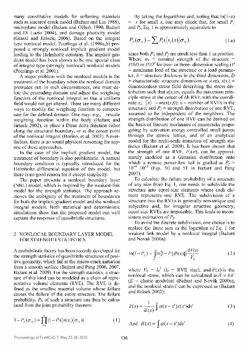
The main obstacle, however, is the treatment of the weight function when the nonlocal domain pro-trudes through the structure boundary. To overcome this difficulty, the nonlocal boundary layer (NBL) method is now proposed.

Figure 1. Concept of boundary layer approach.

In the NBL method, the structure domain is di-

vided into two parts: a boundary layer Vb with thick-ness h = l0 along all the surfaces (including the crack faces), and an interior domain (Fig. 1). For the inte-rior domain VI, one can use the conventional nonlo-cal model to evaluate the nonlocal stress. Since the boundary of interior domain it at distance l0 away from the structure boundary, the nonlocal domain will not protrude through the boundary. For the boundary layer itself, only the stresses and strains at the points at the middle surface Ωm of the layer are used to calculate the failure probability. Therefore, one may rewrite Equation 2 as:

∫

∫

−+

Ω−=−

Ω

I

m

V

MMNf

V

xVxP

V

xxPhP

0

1

0

10

)(d)]([1ln

)(d)]([1ln)](1ln[

σ

σσ

(6)

As the structure size increases, the nonlocal stress

approaches the local stress, the boundary layer be-comes negligible compared to the structure size, and Equation 6 converges to Equation 2.

To give a simple example, consider a rectangular beam of span -to-depth ratio 3, subjected to pure bending. The stress and strain fields are obtained by the engineering beam theory. We define the nominal strength σN = 6M/bD

2, where M = maximum mo-

ment, D = depth of beam, and b = width of beam. To calculate the failure probability of the beam, five methods are considered here:

1) Divide the beam into a number of RVEs and cal-culate the failure probability by Equation 1. This is the original method based on the weakest link model, which is considered as the benchmark solution.

2) The NBL method as proposed. (Eqs 3-6). 3) Conventional nonlocal approach (Eqs 2-5),

where the weighting function is automatically re-scaled when the nonlocal domain protrudes through the structure boundary.

4) Nonlocal approach with the boundary-correction weighting function proposed by Borino et al. (2003), in which the nonlocal strain is expressed as:

∫ −+⎟⎟⎠

⎞⎜⎜⎝

⎛−=

∞

V

xxxx

x

x

x

x 'd)'()'()(

1)(

)(1)( εα

α

ε

α

α

ε (7)

Here

∞α = value of )(xα if the nonlocal domain

does not protrude through the boundary. 5) Nonlocal approach in which a Dirac delta

function is introduced at the structure boundary to compensate for the protruding part of the weight function;

⎥⎦

⎤⎢⎣

⎡+−= ∫∫

Γ∞

yyxxxxxxV

d)()('d)'()'(1

)( εγεαα

ε (8)

and )()()( xxx ααγ −=

∞

where Γ denotes the structure boundary where the nonlocal domain protrudes.

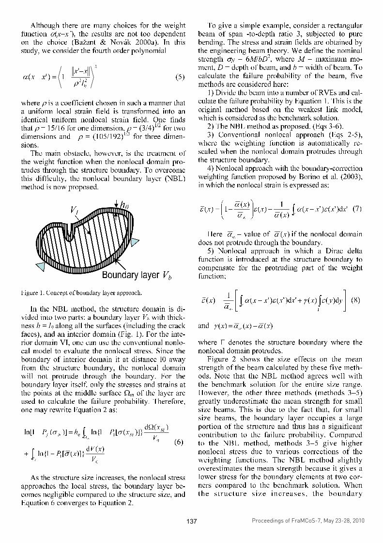
Figure 2 shows the size effects on the mean strength of the beam calculated by these five meth-ods. Note that the NBL method agrees well with the benchmark solution for the entire size range. However, the other three methods (methods 3–5) greatly underestimate the mean strength for small size beams. This is due to the fact that, for small size beams, the boundary layer occupies a large portion of the structure and thus has a significant contribution to the failure probability. Compared to the NBL method, methods 3–5 give higher nonlocal stress due to various corrections of the weighting functions. The NBL method slightly overestimates the mean strength because it gives a lower stress for the boundary elements at two cor-ners compared to the benchmark solution. When the structure size increases, the boundary


hThD ∇−= ),(J (1)


J•∇=∂

∂−

t

w (2)



nscw

s

ew

c

ew

hh

Dt

h

h

ew

&&& ++∂

∂

∂

∂

=∇•∇+∂

∂

∂

∂

− αα

αα

)(

(3)




( ) ( )( )

( ) ( )⎥⎥

⎦

⎤

⎢⎢

⎣

⎡

⎥⎥⎥

⎦

⎤

⎢⎢⎢

⎣

⎡

−

−∞

+

−∞

−=

1110

,1

110

11,

1,,

hcc

ge

scK

hcc

ge

scG

sch

ew

αα

αα

αα

αααα

(4)


( ) ss

s

vgkc

c

c

vgk

scG αααα +=,1

(5)

where k

cvg and k



( )1

110

110

11

22.0188.00

,1

−⎟⎠

⎞⎜⎝

⎛−∞

⎥⎥⎥

⎦

⎤

⎢⎢⎢

⎣

⎡⎟⎠

⎞⎜⎝

⎛−∞

−−+−

=

hcc

ge

hcc

geGs

ssc

w

scK

αα

αα

αα

αα

(6)


cvg and k

svg and g1 can




T∇−= λq (7)


\ _II ")

137

Figure 2. Mean size effect on flexural strength.

layer becomes negligible and the nonlocal strain ap-proaches the local strain. Therefore, all these meth-ods eventually give the same result for large size beams.

3 BOUNDARY LAYER APPROACH FOR GRADIENT MODEL

Inspired by the NBL method for the strength statis-tics, now we apply this concept to the deterministic nonlocal model. In this section, we present the ap-plication of the NBL method to the implicit gradient model proposed by Peerlings et al. (1996a,b, 2001), in which the nonlocal quantity is calculated from the Helmholtz equation (Peerlings et al. 1996 a,b, 2001).

First let us compare the NBL with the original implicit gradient model by analyzing a bar under uniaxial tension and a beam under three-point bend-ing. For the constitutive law, we adopt a simple nonlocal isotropic damage law, which can be de-scribed as:

klijklij C εωσ )1( −=

(9)

where σij = Cauchy stress tensor, εkl = strain tensor, Cijkl = elastic constant, ω = damage parameter. The

damage parameter can be expressed as a function of history parameter κ, which represents the most se-vere deformation the material has experienced. Two commonly used functions are the linear and expo-nential damage laws:

linear:

⎪⎩

⎪⎨

⎧

>

≤≤−

−

=

)(1

)()(

0

0

00

f

f

f

εκ

εκε

εε

εκ

κ

ε

κω

(10a)

exponential:

⎪⎩

⎪⎨

⎧

>⎟⎟

⎠

⎞

⎜⎜

⎝

⎛

−

−−−

≤

=)(exp1

)(0

)(0

0

00

0

εκ

εε

εκ

κ

ε

εκ

κω

f

(10b)

where ε0 = ft/E = the strain at peak stress under uni-axial tension, and εf controls the slope of the soften-ing part of the uniaxial stress-strain curve. Parameter εf can be determined from the area under the uniax-ial stress-strain curve, which is equal to the energy dissipated by the failure process per unit volume.

A scalar equivalent strain εeq is used as a measure of the deformation (Mazars and Pijaudier-Cabot 1989):

∑=

=

3

1

3

i

ieqεε (11)

In the nonlocal version of the damage mechanics,

the damage loading function κε −=eq

f satisfies the following loading conditions:

0),( ≤eq

f εκ ; 0≥κ& , 0),( =

eqf εκκ&

(12)

where eqε is the nonlocal equivalent strain, which

can be calculated from the Helmholtz equation:

eqeqeqc εεε =∇−

22

(13)

(Peerlings et al. 1996a,b, 2001). Parameter c is re-

lated to the size of the nonlocal influence zone for the integral type nonlocal model as (Bažant 1984, Bažant and Planas 1998):

0

2/1

3

0

2

d)( lsl

ssc ⎥

⎦

⎤⎢⎣

⎡= ∫

∞+

∞−

α (14)

If we use the fourth order polynomial as the

weight function (Eq. 5), then we obtain c = 0.271l0. To solve Eq. 13, we need boundary conditions.

Peerlings et al. (1996a,b, 2001) suggested using the natural boundary condition 0/ =∂∂ n

eqε , where n

= unit normal at the boundary. For the FEM imple-


hThD ∇−= ),(J (1)


J•∇=∂

∂−

t

w (2)



nscw

s

ew

c

ew

hh

Dt

h

h

ew

&&& ++∂

∂

∂

∂

=∇•∇+∂

∂

∂

∂

− αα

αα

)(

(3)




( ) ( )( )

( ) ( )⎥⎥

⎦

⎤

⎢⎢

⎣

⎡

⎥⎥⎥

⎦

⎤

⎢⎢⎢

⎣

⎡

−

−∞

+

−∞

−=

1110

,1

110

11,

1,,

hcc

ge

scK

hcc

ge

scG

sch

ew

αα

αα

αα

αααα

(4)


( ) ss

s

vgkc

c

c

vgk

scG αααα +=,1

(5)

where k

cvg and k



( )1

110

110

11

22.0188.00

,1

−⎟⎠

⎞⎜⎝

⎛−∞

⎥⎥⎥

⎦

⎤

⎢⎢⎢

⎣

⎡⎟⎠

⎞⎜⎝

⎛−∞

−−+−

=

hcc

ge

hcc

geGs

ssc

w

scK

αα

αα

αα

αα

(6)


cvg and k

svg and g1 can




T∇−= λq (7)


1.2

0.8

onventional nonlocal Borino Dirac delta function

0.4 -+-----.----------r-------'

o

- 6 -r--------------, (I N

5

NBL

ventional nonlocal Bor 0

4 Dirac elta function

3

2~---._---._---~

2 8

odel

11-

138

mentation, it was proposed to solve the weak forms of equilibrium equation and the Helmholtz equation jointly (de Borst and Mühlhaus 1992, Peerlings et al. 1996a). The physical interpretation of the natural boundary condition still remains unclarified, which appears to be the major drawback of the gradient model. (Peerlings et al 1996a, 2001).

When the NBL for the implicit gradient model is adopted, the Helmholtz equation needs to be solved for the interior domain only. The boundary condition along the interface between the interior domain and the boundary layer involves both the force and natu-ral boundary conditions:

beqeq

eq

n

h

,

0

2εε

ε

=+∂

∂

(14)

where εeq,b = equivalent strain at middle surface of the boundary layer, and n = unit normal of the inter-face. Eq. 14 ha a clear physical meaning —continuity of the nonlocal equivalent strain field across the interface between the interior domain and the boundary layer.

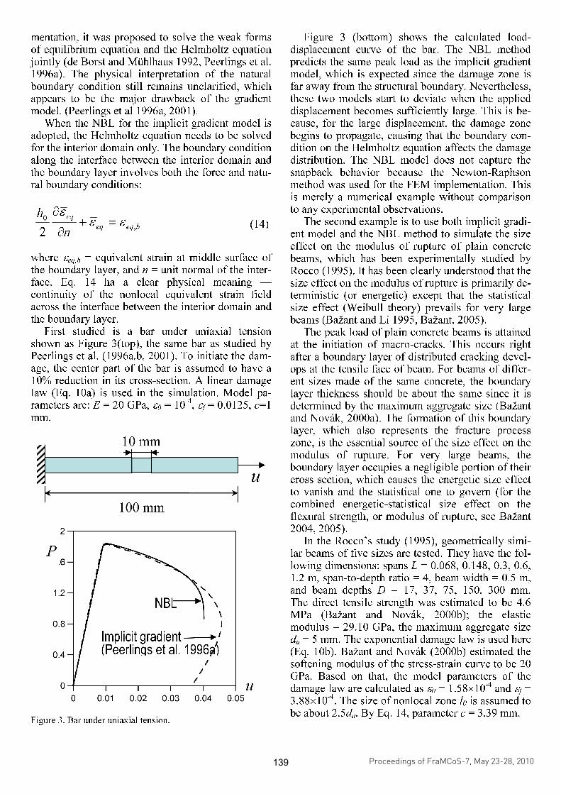
First studied is a bar under uniaxial tension shown as Figure 3(top), the same bar as studied by Peerlings et al. (1996a,b, 2001). To initiate the dam-age, the center part of the bar is assumed to have a 10% reduction in its cross-section. A linear damage law (Eq. 10a) is used in the simulation. Model pa-rameters are: E = 20 GPa, ε0 = 10

-4, εf = 0.0125, c=1

mm.

Figure 3. Bar under uniaxial tension.

Figure 3 (bottom) shows the calculated load-displacement curve of the bar. The NBL method predicts the same peak load as the implicit gradient model, which is expected since the damage zone is far away from the structural boundary. Nevertheless, these two models start to deviate when the applied displacement becomes sufficiently large. This is be-cause, for the large displacement, the damage zone begins to propagate, causing that the boundary con-dition on the Helmholtz equation affects the damage distribution. The NBL model does not capture the snapback behavior because the Newton-Raphson method was used for the FEM implementation. This is merely a numerical example without comparison to any experimental observations.

The second example is to use both implicit gradi-ent model and the NBL method to simulate the size effect on the modulus of rupture of plain concrete beams, which has been experimentally studied by Rocco (1995). It has been clearly understood that the size effect on the modulus of rupture is primarily de-terministic (or energetic) except that the statistical size effect (Weibull theory) prevails for very large beams (Bažant and Li 1995, Bažant, 2005).

The peak load of plain concrete beams is attained at the initiation of macro-cracks. This occurs right after a boundary layer of distributed cracking devel-ops at the tensile face of beam. For beams of differ-ent sizes made of the same concrete, the boundary layer thickness should be about the same since it is determined by the maximum aggregate size (Bažant and Novák, 2000a). The formation of this boundary layer, which also represents the fracture process zone, is the essential source of the size effect on the modulus of rupture. For very large beams, the boundary layer occupies a negligible portion of their cross section, which causes the energetic size effect to vanish and the statistical one to govern (for the combined energetic-statistical size effect on the flexural strength, or modulus of rupture, see Bažant 2004, 2005).

In the Rocco’s study (1995), geometrically simi-lar beams of five sizes are tested. They have the fol-lowing dimensions: spans L = 0.068, 0.148, 0.3, 0.6, 1.2 m, span-to-depth ratio = 4, beam width = 0.5 m, and beam depths D = 17, 37, 75, 150, 300 mm. The direct tensile strength was estimated to be 4.6 MPa (Bažant and Novák, 2000b); the elastic modulus = 29.10 GPa, the maximum aggregate size da = 5 mm. The exponential damage law is used here (Eq. 10b). Bažant and Novák (2000b) estimated the softening modulus of the stress-strain curve to be 20 GPa. Based on that, the model parameters of the damage law are calculated as ε0 = 1.58×10

-4 and εf =

3.88×10-4

. The size of nonlocal zone l0 is assumed to be about 2.5da. By Eq. 14, parameter c = 3.39 mm.


hThD ∇−= ),(J (1)


J•∇=∂

∂−

t

w (2)



nscw

s

ew

c

ew

hh

Dt

h

h

ew

&&& ++∂

∂

∂

∂

=∇•∇+∂

∂

∂

∂

− αα

αα

)(

(3)




( ) ( )( )

( ) ( )⎥⎥

⎦

⎤

⎢⎢

⎣

⎡

⎥⎥⎥

⎦

⎤

⎢⎢⎢

⎣

⎡

−

−∞

+

−∞

−=

1110

,1

110

11,

1,,

hcc

ge

scK

hcc

ge

scG

sch

ew

αα

αα

αα

αααα

(4)


( ) ss

s

vgkc

c

c

vgk

scG αααα +=,1

(5)

where k

cvg and k



( )1

110

110

11

22.0188.00

,1

−⎟⎠

⎞⎜⎝

⎛−∞

⎥⎥⎥

⎦

⎤

⎢⎢⎢

⎣

⎡⎟⎠

⎞⎜⎝

⎛−∞

−−+−

=

hcc

ge

hcc

geGs

ssc

w

scK

αα

αα

αα

αα

(6)


cvg and k

svg and g1 can




T∇−= λq (7)


~1-________ Io~m~m ______ ~lu ~ ~ "I I" ,----1<

IOOmm

2~------------------~

P .6

1.2

0.8

0.4

" NB~\ \ I

Implicit gradient ~ I (Peerlinqs et al. 1996911

O~--~--~--~--~--~

o 0.01 0 .02 0.03 0.04 0.05 u

139

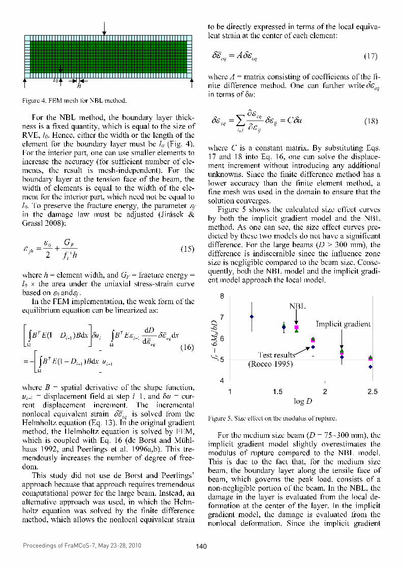
Figure 4. FEM mesh for NBL method.

For the NBL method, the boundary layer thick-

ness is a fixed quantity, which is equal to the size of RVE, l0. Hence, either the width or the length of the element for the boundary layer must be l0 (Fig. 4). For the interior part, one can use smaller elements to increase the accuracy (for sufficient number of ele-ments, the result is mesh-independent). For the boundary layer at the tension face of the beam, the width of elements is equal to the width of the ele-ment for the interior part, which need not be equal to l0. To preserve the fracture energy, the parameter εf in the damage law must be adjusted (Jirásek & Grassl 2008):

hf

G

t

F

fh'2

0+=

ε

ε (15)

where h = element width, and GF = fracture energy = l0 × the area under the uniaxial stress-strain curve based on ε0 andεf .

In the FEM implementation, the weak form of the equilibrium equation can be linearized as:

11

11

d)1(

dd

dd)1(

−

Ω

−

Ω

−

Ω

−

⎥⎦

⎤⎢⎣

⎡−−=

−⎥⎦

⎤⎢⎣

⎡−

∫

∫∫

ii

T

eq

eq

i

T

ii

T

uxBDEB

xD

EBuxBDEB εδε

εδ

(16)

where B = spatial derivative of the shape function, ui−1 = displacement field at step i−1, and δu = cur-rent displacement increment. The incremental nonlocal equivalent strain

eqεδ is solved from the

Helmholtz equation (Eq. 13). In the original gradient method, the Helmholtz equation is solved by FEM, which is coupled with Eq. 16 (de Borst and Mühl-haus 1992, and Peerlings et al. 1996a,b). This tre-mendously increases the number of degree of free-dom.

This study did not use de Borst and Peerlings’ approach because that approach requires tremendous computational power for the large beam. Instead, an alternative approach was used, in which the Helm-holtz equation was solved by the finite difference method, which allows the nonlocal equivalent strain

to be directly expressed in terms of the local equiva-lent strain at the center of each element:

eqeqAδεεδ = (17)

where A = matrix consisting of coefficients of the fi-nite difference method. One can further write

eqδε

in terms of δu:

∑ =∂

∂=

ji

ij

ij

eq

equC

,

δδεε

εδε (18)

where C is a constant matrix. By substituting Eqs. 17 and 18 into Eq. 16, one can solve the displace-ment increment without introducing any additional unknowns. Since the finite difference method has a lower accuracy than the finite element method, a fine mesh was used in the domain to ensure that the solution converges.

Figure 5 shows the calculated size effect curves by both the implicit gradient model and the NBL method. As one can see, the size effect curves pre-dicted by these two models do not have a significant difference. For the large beams (D > 300 mm), the difference is indiscernible since the influence zone size is negligible compared to the beam size. Conse-quently, both the NBL model and the implicit gradi-ent model approach the local model.

Figure 5. Size effect on the modulus of rupture.

For the medium size beam (D = 75~300 mm), the

implicit gradient model slightly overestimates the modulus of rupture compared to the NBL model. This is due to the fact that, for the medium size beam, the boundary layer along the tensile face of beam, which governs the peak load, consists of a non-negligible portion of the beam. In the NBL, the damage in the layer is evaluated from the local de-formation at the center of the layer. In the implicit gradient model, the damage is evaluated from the nonlocal deformation. Since the implicit gradient


hThD ∇−= ),(J (1)


J•∇=∂

∂−

t

w (2)



nscw

s

ew

c

ew

hh

Dt

h

h

ew

&&& ++∂

∂

∂

∂

=∇•∇+∂

∂

∂

∂

− αα

αα

)(

(3)




( ) ( )( )

( ) ( )⎥⎥

⎦

⎤

⎢⎢

⎣

⎡

⎥⎥⎥

⎦

⎤

⎢⎢⎢

⎣

⎡

−

−∞

+

−∞

−=

1110

,1

110

11,

1,,

hcc

ge

scK

hcc

ge

scG

sch

ew

αα

αα

αα

αααα

(4)


( ) ss

s

vgkc

c

c

vgk

scG αααα +=,1

(5)

where k

cvg and k



( )1

110

110

11

22.0188.00

,1

−⎟⎠

⎞⎜⎝

⎛−∞

⎥⎥⎥

⎦

⎤

⎢⎢⎢

⎣

⎡⎟⎠

⎞⎜⎝

⎛−∞

−−+−

=

hcc

ge

hcc

geGs

ssc

w

scK

αα

αα

αα

αα

(6)


cvg and k

svg and g1 can




T∇−= λq (7)


8

NFL + i Implicit gradient

Test result~t ~ '* (Rocco 1995) ~

7

2 ---~6 \0

II

~5

4

1.5 2 2.5 logD

140

hfG tfF '2

1ε=

model is mesh-insensitive, considering the same mesh for both methods, the implicit gradient model gives a slightly lower damage value, and thus a higher peak load, than the NBL method does. It seems that the NBL gives slightly better prediction compared to the test data.

For the small size beam (D < 75 mm), the trend of the NBL method greatly overestimates the modulus of rupture. This is due to the fact that the NBL method limits the element size for the bound-ary layer (Fig. 4). For the small beam, this layer can occupy one fourth to one half of the beam depth. This causes that there are too few elements along the beam depth. In such a case, the beam is too stiff and the peak load is greatly overestimated due to the numerical errors. Therefore, the NBL method is not suitable when the beam is too small, i.e. the depth of beam is less than 4 RVEs.

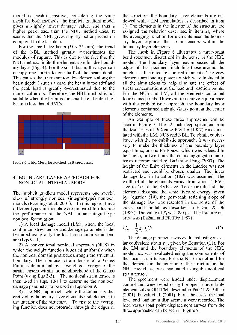
Figure 6. FEM Mesh for notched TPB specimens.

4 BOUNDARY LAYER APPROACH FOR NONLOCAL INTEGRAL MODEL

The implicit gradient model represents one special class of strongly nonlocal (integral-type) nonlocal models (Peerlings et al. 2001). In this regard, three different types of models were prepared to illustrate the performance of the NBL in an integral-type nonlocal formulation:

1) A local damage model (LM), where the local continuum stress tensor and damage parameter is de-termined using only the local continuum strain ten-sor (Eqs 9-11).

2) A conventional nonlocal approach (NUS) in which the weight function is scaled uniformly when the nonlocal domain protrudes through the structural boundary. The nonlocal strain tensor at a Gauss Point is determined by a weighted average of the strain tensors within the neighborhood of the Gauss Point (using Eqs 3-5). The nonlocal strain tensor is then used in Eqs. 10-11 to determine the nonlocal damage parameter to be used in Equation 9.

3) The NBL approach, where the domain is dis-cretized by boundary layer elements and elements in the interior of the structure. To ensure the averag-ing function does not protrude through the edges of

the structure, the boundary layer elements are en-dowed with a LM formulation as described in item 1). The elements in the interior of the structure are assigned the behavior described in item 2), where the averaging function for elements near the bound-ary layer captures the strain tensors within the boundary layer elements.

The mesh in Figure 6 illustrates a three-point bend specimen discretized in the sense or the NBL model. The boundary layer encompasses all the edges of the specimen, including those around the notch, as illustrated by the red elements. The grey elements are loading platens which were included in all the simulations to help eliminate the effect of stress concentrations at the load and reaction points. For the NUS and LM, all the elements contained four Gauss points. However, to achieve equivalence with the probabilistic approach, the boundary layer elements contained a single Gauss point at the center of the elements.

An example of these three approaches can be seen in Figure 7. The 12 inch deep specimen from the test series of Bažant & Pfeiffer (1987) was simu-lated with the LM, NUS and NBL. To obtain equiva-lence with the probabilistic approach, it was neces-sary to make the thickness of the boundary layer equal to l0, or one RVE size, which was selected to be 1 inch, or two times the coarse aggregate diame-ter as recommended by Bažant & Pang (2007). The height of the finite elements in the interior was not restricted and could be chosen smaller. The linear damage law in Equation (10a) was assumed. The width of all the elements varied from about 1 RVE size to 1/3 of the RVE size. To ensure that all the elements dissipate the same fracture energy, given by Equation (19), the post-peak softening slope of the damage law was rescaled in the sense of the crack band model, as described in Bažant & Oh (1983). The value of f't was 390 psi. The fracture en-ergy was (Bažant and Pfeiffer 1987):

(19)

The damage parameter was evaluated using a sca-

lar equivalent strain εeq, given by Equation (11). For the LM and the boundary elements of the NBL model, εeq was evaluated using the components of the local strain tensor. For the NUS model and for the elements in the interior of the structure in the NBL model, εeq was evaluated using the nonlocal strain tensor.

The specimens were loaded under displacement control and were tested using the open source finite element solver OOFEM, descried in Patzák & Bittnar (2001), Patzák et al. (2001). In all the cases, the load level and load point displacement were recorded. The load versus load point displacement curves from the three approaches can be seen in Figure 7.


hThD ∇−= ),(J (1)


J•∇=∂

∂−

t

w (2)



nscw

s

ew

c

ew

hh

Dt

h

h

ew

&&& ++∂

∂

∂

∂

=∇•∇+∂

∂

∂

∂

− αα

αα

)(

(3)




( ) ( )( )

( ) ( )⎥⎥

⎦

⎤

⎢⎢

⎣

⎡

⎥⎥⎥

⎦

⎤

⎢⎢⎢

⎣

⎡

−

−∞

+

−∞

−=

1110

,1

110

11,

1,,

hcc

ge

scK

hcc

ge

scG

sch

ew

αα

αα

αα

αααα

(4)


( ) ss

s

vgkc

c

c

vgk

scG αααα +=,1

(5)

where k

cvg and k



( )1

110

110

11

22.0188.00

,1

−⎟⎠

⎞⎜⎝

⎛−∞

⎥⎥⎥

⎦

⎤

⎢⎢⎢

⎣

⎡⎟⎠

⎞⎜⎝

⎛−∞

−−+−

=

hcc

ge

hcc

geGs

ssc

w

scK

αα

αα

αα

αα

(6)


cvg and k

svg and g1 can




T∇−= λq (7)


141

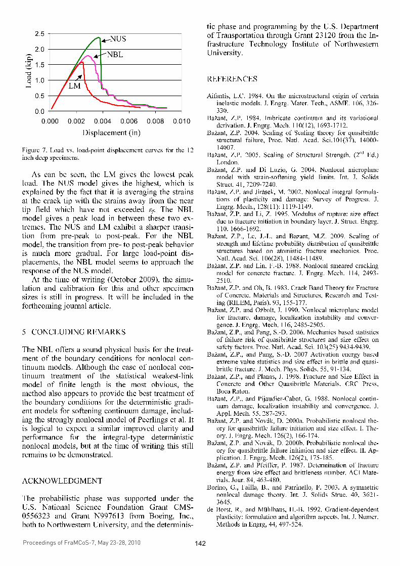
Figure 7. Load vs. load-point displacement curves for the 12 inch deep specimens.

As can be seen, the LM gives the lowest peak

load. The NUS model gives the highest, which is explained by the fact that it is averaging the strains at the crack tip with the strains away from the near tip field which have not exceeded εf. The NBL model gives a peak load in between these two ex-tremes. The NUS and LM exhibit a sharper transi-tion from pre-peak to post-peak. For the NBL model, the transition from pre- to post-peak behavior is much more gradual. For large load-point dis-placements, the NBL model seems to approach the response of the NUS model.

At the time of writing (October 2009), the simu-lation and calibration for this and other specimen sizes is still in progress. It will be included in the forthcoming journal article.

5 CONCLUDING REMARKS

The NBL offers a sound physical basis for the treat-ment of the boundary conditions for nonlocal con-tinuum models. Although the case of nonlocal con-tinuum treatment of the statistical weakest-link model of finite length is the most obvious, the method also appears to provide the best treatment of the boundary conditions for the deterministic gradi-ent models for softening continuum damage, includ-ing the strongly nonlocal model of Peerlings et al. It is logical to expect a similar improved clarity and performance for the integral-type deterministic nonlocal models, but at the time of writing this still remains to be demonstrated.

ACKNOWLEDGMENT

The probabilistic phase was supported under the U.S. National Science Foundation Grant CMS-0556323 and Grant N997613 from Boeing, Inc., both to Northwestern University, and the determinis-

tic phase and programming by the U.S. Department of Transportation through Grant 23120 from the In-frastructure Technology Institute of Northwestern University.

REFERENCES

Aifantis, E.C. 1984. On the microstructural origin of certain inelastic models. J. Engrg. Mater. Tech., ASME. 106, 326-330.

Bažant, Z.P. 1984. Imbricate continuum and its variational derivation. J. Engrg. Mech. 110(12), 1693-1712.

Bažant, Z.P. 2004. Scaling of Scaling theory for quasibrittle structural failure, Proc. Natl. Acad. Sci.101(37), 14000-14007.

Bažant, Z.P. 2005. Scaling of Structural Strength. (2nd Ed.) London.

Bažant, Z.P. and Di Luzio, G. 2004. Nonlocal microplane model with strain-softening yield limits. Int. J. Solids Struct. 41, 7209-7240.

Bažant, Z.P. and Jirásek, M. 2002. Nonlocal integral formula-tions of plasticity and damage: Survey of Progress. J. Engrg. Mech., 128(11): 1119-1149.

Bažant, Z.P. and Li, Z. 1995. Modulus of rupture: size effect due to fracture initiation in boundary layer. J. Struct. Engrg. 110. 1666-1692.

Bažant, Z.P., Le, J.-L. and Bazant, M.Z. 2009. Scaling of strength and lifetime probability distribution of quasibrittle structures based on atomistic fracture mechanics. Proc. Natl. Acad. Sci. 106(28), 11484-11489.

Bažant, Z.P. and Lin, F.-B. 1988. Nonlocal smeared cracking model for concrete fracture. J. Engrg. Mech. 114, 2493-2510.

Bažant, Z.P. and Oh, B. 1983. Crack Band Theory for Fracture of Concrete. Materials and Structures, Research and Test-ing (RILEM, Paris). 93, 155-177.

Bažant, Z.P. and Ožbolt, J. 1990. Nonlocal microplane model for fracture, damage, localization instability and conver-gence. J. Engrg. Mech. 116, 2485-2505.

Bažant, Z.P., and Pang, S.-D. 2006. Mechanics based statistics of failure risk of quasibrittle structures and size effect on safety factors. Proc. Natl. Acad. Sci. 103(25) 9434-9439.

Bažant, Z.P., and Pang, S.-D. 2007 Activation energy based extreme value statistics and size effect in brittle and quasi-brittle fracture. J. Mech. Phys. Solids. 55, 91-134.

Bažant, Z.P., and Planas, J. 1998. Fracture and Size Effect in Concrete and Other Quasibrittle Materials. CRC Press, Boca Raton.

Bažant, Z.P., and Pijaudier-Cabot, G. 1988. Nonlocal contin-uum damage, localization instability and convergence. J. Appl. Mech. 55, 287-293.

Bažant, Z.P. and Novák, D. 2000a. Probabilistic nonlocal the-ory for quasibrittle failure initiation and size effect. I. The-ory. J. Engrg. Mech. 126(2), 166-174.

Bažant, Z.P. and Novák, D. 2000b. Probabilistic nonlocal the-ory for quasibrittle failure initiation and size effect. II. Ap-plication. J. Engrg. Mech. 126(2), 175-185.

Bažant, Z.P. and Pfeiffer, P. 1987. Determination of fracture energy from size effect and brittleness number. ACI Mate-rials. Jour. 84, 463-480.

Borino, G., Failla, B., and Parrinello, F. 2003. A symmetric nonlocal damage theory. Int. J. Solids Struc. 40, 3621-3645.

de Borst, R., and Mühlhaus, H.-B. 1992. Gradient-dependent plasticity: formulation and algorithm aspects. Int. J. Numer. Methods in Engrg, 44, 497-524.


hThD ∇−= ),(J (1)


J•∇=∂

∂−

t

w (2)



nscw

s

ew

c

ew

hh

Dt

h

h

ew

&&& ++∂

∂

∂

∂

=∇•∇+∂

∂

∂

∂

− αα

αα

)(

(3)




( ) ( )( )

( ) ( )⎥⎥

⎦

⎤

⎢⎢

⎣

⎡

⎥⎥⎥

⎦

⎤

⎢⎢⎢

⎣

⎡

−

−∞

+

−∞

−=

1110

,1

110

11,

1,,

hcc

ge

scK

hcc

ge

scG

sch

ew

αα

αα

αα

αααα

(4)


( ) ss

s

vgkc

c

c

vgk

scG αααα +=,1

(5)

where k

cvg and k



( )1

110

110

11

22.0188.00

,1

−⎟⎠

⎞⎜⎝

⎛−∞

⎥⎥⎥

⎦

⎤

⎢⎢⎢

⎣

⎡⎟⎠

⎞⎜⎝

⎛−∞

−−+−

=

hcc

ge

hcc

geGs

ssc

w

scK

αα

αα

αα

αα

(6)


cvg and k

svg and g1 can




T∇−= λq (7)


2.5 .,-----------------,

2.0 +-------j'----+-----------1 ~

0.. ;g 1.5 +-------J.lF+---t-+-----------1

'"0 i3 1.0 +------.~<....:....+--\:I-----------1 ~

0.5 +--1----~-~,_____--------1

0.0 +------,-----,------.----,-------1

- 0.000 0.002 0.004 0.006 0.008 0.010

Displacement (in)

142

Eringen, A.C. 1965. Theory of micropolar continuum. In Proc., Ninth Midwestern Mechanics Conference, 23-40.

Eringen, A.C. 1966. A unified theory of thermomechanical ma-terials. Int. J. Mech. Phys. 44, 497-524.

Grassl, P. and Jirásek, M. 2006 Plastic model with non-local damage applied to concrete. Int. J. Numer. Anal. Methods in Geomachnics. 30, 71-90.

Jirásek, M. 1997. Nonlocal models for damage and fracture: comparison of approaches. Int. J. Solids Struc. 35(31), 4133-4145.

Jirásek, M. and Grassl, P. 2008 Evaluation of directional mesh bias in concrete fracture simulations using continuum dam-age mechanics. Engrg. Frac. Mech. 75, 1921-1943.

Kröner, E. 1967. Elasticity theory of materials with long-range cohesive forces. Int. J. Solids Struc. 3, 731-742.

Mazars, J. and Pijaudier-Cabot, G. 1989 Continuum damage theory-application to concrete. J. Engrg. Mech. 115(2) 345-365.

Patzák, B. and Bittnar, Z. 2001 Design of object oriented finite element code. Advances in Engineering Software. 32(10-11):759-767.

Patzák, B., Rypl, D. and Bittnar, Z. 2001 Parallel explicit finite element dynamics with nonlocal constitutive models. Com-puters and Structures. 79(26-28):2287-2297.

Peerlings, R.H.J., de Borst, R., Brekelmans, W.A.M., and De Vree, J.H.P. 1996. Gradient enhanced damage for qusi-brittle materials. Int. J. Numer. Methods in Engrg, 39, 3391-3403.

Peerlings, R.H.J., de Borst, R., Brekelmans, W.A.M., De Vree, J.H.P., and Spee, I. 1996. Some observations on localiza-tion in non-local and gradient damage models. Eur. J. Mech., A/Solids. 6, 937-953.

Peerlings, R.H.J., Geers, M.G.D., de Borst, R., and Brekel-mans, W.A.M. 2001. A critical comparison of nonlocal and gradient-enhanced softening continua. Int. J. Solids Struc., 38, 7723-7746.

Pijaudier-Cabot, G. and Bažant, Z.P., 1987. Nonlocal damage theory. J.Engrg. Mech. 113(10) 1512-1533.

Rocco, C.G. 1995, Size dependence and fracture mechanisms in the diagonal compression splitting test. PhD thesis, Dept. Ciencia de Materiales, Universidad Politecnica de Madrid.

Triantafyllidis, N., and Aifantis, E. 1986. A gradient approach to localization of deformation. I. Hyperelastic materials. J. Elasticity. 16, 225-237.


hThD ∇−= ),(J (1)


J•∇=∂

∂−

t

w (2)



nscw

s

ew

c

ew

hh

Dt

h

h

ew

&&& ++∂

∂

∂

∂

=∇•∇+∂

∂

∂

∂

− αα

αα

)(

(3)




( ) ( )( )

( ) ( )⎥⎥

⎦

⎤

⎢⎢

⎣

⎡

⎥⎥⎥

⎦

⎤

⎢⎢⎢

⎣

⎡

−

−∞

+

−∞

−=

1110

,1

110

11,

1,,

hcc

ge

scK

hcc

ge

scG

sch

ew

αα

αα

αα

αααα

(4)


( ) ss

s

vgkc

c

c

vgk

scG αααα +=,1

(5)

where k

cvg and k



( )1

110

110

11

22.0188.00

,1

−⎟⎠

⎞⎜⎝

⎛−∞

⎥⎥⎥

⎦

⎤

⎢⎢⎢

⎣

⎡⎟⎠

⎞⎜⎝

⎛−∞

−−+−

=

hcc

ge

hcc

geGs

ssc

w

scK

αα

αα

αα

αα

(6)


cvg and k

svg and g1 can




T∇−= λq (7)


143

Documents

Nonlocal boundary layer (NBL) model: overcoming … · Zdenk. P. Ba ant, Jia-Liang Le & Christian G. Hoover Northwestern University, IL, USA. ABSTRACT: Applications of the nonlocal