Embed Size (px)
Citation preview

NONPARAMETRIC AND SEMIPARAMETRIC METHODS IN R
JEFFREY S. RACINE
Abstract. The R environment for statistical computing and graphics (R Development Core Team(2008)) offers practitioners a rich set of statistical methods ranging from random number genera-tion and optimization methods through regression, panel data, and time series methods, by way ofillustration. The standard R distribution (‘base R) comes preloaded with a rich variety of function-ality useful for applied econometricians. This functionality is enhanced by user supplied packagesmade available via R servers that are mirrored around the world. Of interest in this chapter aremethods for estimating nonparametric and semiparametric models. We summarize many of thefacilities in R and consider some tools that might be of interest to those wishing to work withnonparametric methods who want to avoid resorting to programming in C or Fortran but need thespeed of compiled code as opposed to interpreted code such as Gauss or Matlab by way of example.We encourage those working in the field to strongly consider implementing their methods in theR environment thereby making their work accessible to the widest possible audience via an opencollaborative forum.
1. Introduction
Unlike their more established parametric counterparts, many nonparametric and semiparametric
methods that have received widespread theoretical treatment have not yet found their way into
mainstream commercial packages. This has hindered their adoption by applied researchers, and it
is safe to describe the availability of modern nonparametric methods as fragmented at best, which
can be frustrating for users who wish to assess whether or not such methods can add value to their
application. Thus, one frequently heard complaint about the state of nonparametric kernel methods
concerns the lack of software along with the fact that implementations in interpreted environments
such as Gauss are orders of magnitude slower than compiled implementations written in C or
Fortran. Though many researchers may code their methods, often using interpreted environments
such as Gauss, it is fair to characterize much of this code as neither designed nor suited as tools
for general purpose use as they are typically written solely to demonstrate ‘proof of concept’. Even
though many authors are more than happy to circulate such code (which is of course appreciated!),
this often imposes certain hardships on the user including 1) having to purchase a (closed and
proprietary) commercial software package and 2) having to modify the code substantially in order
to use it for their application.
The R environment for statistical computing and graphics (R Development Core Team (2008))
offers practitioners a range of tools for estimating nonparametric, semiparametric, and of course
parametric models. Unlike many commercial programs, which must first be purchased in order to
evaluate them, you can adopt R with minimal effort and with no financial outlay required. Many
Date: November 14, 2008.
1
2 JEFFREY S. RACINE
nonparametric methods are well documented, tested, and are suitable for general use via a common
interface structure (such as the ‘formula’ interface) making it easy for users familiar with R to deploy
these tools for their particular application. Furthermore, one of the strengths of R is the ability
to call compiled C or Fortran code via a common interface structure thereby delivering the speed
of complied code in a flexible easy to use environment. In addition, there exist a number of R
‘packages’ (often called ‘libraries’ or ‘modules’ in other environments) that implement a variety of
kernel methods, albeit with varying degrees of functionality (e.g., univariate versus multivariate,
the ability/inability to handle numerical and categorical data and so forth). Finally, R delivers a
rich framework for implementing and making code available to the community.
In this chapter we outline many of the functions and packages available in R that might be
of interest to practitioners, and consider some illustrative applications along with code fragments
that might be of interest. Before proceeding further, we first begin with an introduction to the R
environment itself.
2. The R Environment
What is R? Perhaps it is best to begin with the question “what is S”? S is a language and en-
vironment designed for statical computing and graphics which was developed at Bell Laboratories
(formerly AT&T, now Lucent Technologies). S has grown to become the de-facto standard among
econometricians and statisticians, and there are two main implementations, the commercial imple-
mentation called ‘S-PLUS’, and the free, open-source implementation called ‘R’. R delivers a rich
array of statistical methods, and one of its strengths is the ease with which ‘packages’ can be de-
veloped and made available to users for free. R is a mature open platform that is ideally suited to
the task of making ones method available to the widest possible user base free of charge.
In this section we briefly describe a handful of resources available to those interested in using
R, introduce the user to the R environment, and introduce the user to the foreign package that
facilitates importation of data from packages such as SAS, SPSS, Stata, and Minitab, among others.
2.1. Web sites. A number of sites are devoted to helping R users, and we briefly mention a few of
them below.
http://www.R-project.org/: This is the R home page from which you can download the
program itself and many R packages. There are also manuals, other links, and facilities for
joining various R mailing lists.
http://CRAN.R-project.org/: This is the ‘Comprehensive R Archive Network,’ “a net-
work of ftp and web servers around the world that store identical, up-to-date, versions of
code and documentation for the R statistical package.” Packages are only put on CRAN
when they pass a rather stringent collection of quality assurance checks, and in particular
are guaranteed to build and run on standard platforms.
http://cran.r-project.org/web/views/Econometrics.html: This is the CRAN ‘task
view’ for computational econometrics. “Base R ships with a lot of functionality useful
NONPARAMETRIC AND SEMIPARAMETRIC METHODS IN R 3
for computational econometrics, in particular in the stats package. This functionality is
complemented by many packages on CRAN, a brief overview is given below.” This provides
an excellent summary of both parametric and nonparametric packages that exist for the R
environment.
http://pj.freefaculty.org/R/Rtips.html: This site provides a large and excellent collec-
tion of R tips.
2.2. Getting started with R. A number of well written manuals exist for R and can be located
at the R web site. This section is clearly not intended to be a substitute for these resources. It
simply provides a minimal set of commands which will aid those who have never used R before.
Having installed and run R, you will find yourself at the > prompt. To quit the program, simply
type q(). To get help, you can either enter a command preceded by a question mark, as in ?help,
or type help.start() at the > prompt. The latter will spawn your web browser (it reads files
from your hard drive, so you do not have to be connected to the Internet to use this feature).
You can enter commands interactively at the R prompt, or you can create a text file con-
taining the commands and execute all commands in the file from the R prompt by typ-
ing source ("commands.R"), where commands.R is the text file containing your commands.
Many editors recognize the .R extension providing useful interface for the development of R
code. For example, GNU Emacs is a powerful editor that works well with R and also LATEX
(http://www.gnu.org/software/emacs/emacs.html).
When you quit by entering the q() command, you will be asked whether or not you wish to save
the current session. If you enter Y, then the next time you run R in the same directory it will load all
of the objects created in the previous session. If you do so, typing the command ls() will list all of
the objects. For this reason, it is wise to use different directories for different projects. To remove
objects that have been loaded, you can use the command rm(objectname) or rm(list=ls()) will
remove all objects in memory.
2.3. Importing data from other formats. The foreign package allows you to read data created
by different popular programs. To load it, simply type library(foreign) from within R. Supported
formats include
read.arff: Read Data from ARFF Files
read.dbf: Read a DBF File
read.dta: Read Stata Binary Files
read.epiinfo: Read Epi Info Data Files
read.mtp: Read a Minitab Portable Worksheet
read.octave: Read Octave Text Data Files
read.S: Read an S3 Binary or data.dump File
read.spss: Read an SPSS Data File
read.ssd: Obtain a Data Frame from a SAS Permanent Dataset, via read.xport
read.systat: Obtain a Data Frame from a Systat File
4 JEFFREY S. RACINE
read.xport: Read a SAS XPORT Format Library
The following code snippet reads the Stata file ‘wage1.dta’ (Wooldridge (2002)) and lists the
names of variables in the data frame.
R> library(foreign)
R> mydat <- read.dta(file="wage1.dta")
R> names(mydat)
[1] "wage" "educ" "exper" "tenure" "nonwhite" "female"
[7] "married" "numdep" "smsa" "northcen" "south" "west"
[13] "construc" "ndurman" "trcommpu" "trade" "services" "profserv"
[19] "profocc" "clerocc" "servocc" "lwage" "expersq" "tenursq"
Clearly R makes it simple to migrate data from one environment to another.
Having installed R and having read in data from a text file or supported format such as a
Stata binary file, you can then install packages via the install.packages() command, as in
install.packages("np") which will install the np package (Hayfield & Racine (2008)).

NONPARAMETRIC AND SEMIPARAMETRIC METHODS IN R 5
3. Some Nonparametric and Semiparametric Routines Available in R
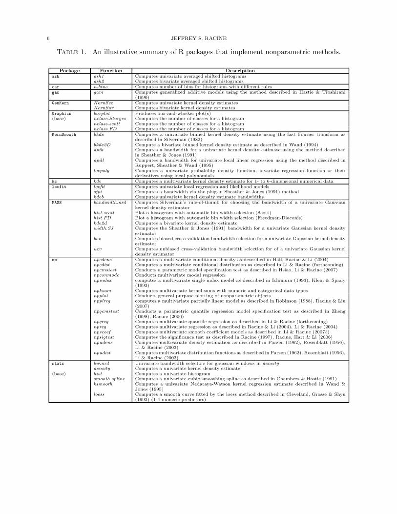
Table 1 summarizes some of the nonparametric and semiparametric routines available to users
of R. As can be seen, there appears to be a rich range of nonparametric implementations avail-
able to the practitioner. However, upon closer inspection many are limited in one way or another
in ways that might frustrate applied econometricians. For instance, some nonparametric regres-
sion methods admit only one regressor, while others admit only numerical data types and cannot
admit categorical data that is often found in applied settings. Table 1 is not intended to be
exhaustive, rather, it ought to serve to orient the reader to a subset of the rich array of nonpara-
metric methods that currently exist in the R environment. To see a routine in action, you can
type example("funcname",package="pkgname") where funcname is the name of a routine and
pkgname is the associated package and this will run an example contained in the help file for that
function. For instance, example("npreg",package="np") will run a kernel regression example
from the package np.
6 JEFFREY S. RACINE
Table 1. An illustrative summary of R packages that implement nonparametric methods.
Package Function Description
ash ash1 Computes univariate averaged shifted histogramsash2 Computes bivariate averaged shifted histograms
car n.bins Computes number of bins for histograms with different rulesgam gam Computes generalized additive models using the method described in Hastie & Tibshirani
(1990)GenKern KernSec Computes univariate kernel density estimates
KernSur Computes bivariate kernel density estimatesGraphics boxplot Produces box-and-whisker plot(s)(base) nclass.Sturges Computes the number of classes for a histogram
nclass.scott Computes the number of classes for a histogramnclass.FD Computes the number of classes for a histogram
KernSmooth bkde Computes a univariate binned kernel density estimate using the fast Fourier transform asdescribed in Silverman (1982)
bkde2D Compute a bivariate binned kernel density estimate as described in Wand (1994)dpik Computes a bandwidth for a univariate kernel density estimate using the method described
in Sheather & Jones (1991)dpill Computes a bandwidth for univariate local linear regression using the method described in
Ruppert, Sheather & Wand (1995)locpoly Computes a univariate probability density function, bivariate regression function or their
derivatives using local polynomialsks kde Computes a multivariate kernel density estimate for 1- to 6-dimensional numerical datalocfit locfit Computes univariate local regression and likelihood models
sjpi Computes a bandwidth via the plug-in Sheather & Jones (1991) methodkdeb Computes univariate kernel density estimate bandwidths
MASS bandwidth.nrd Computes Silverman’s rule-of-thumb for choosing the bandwidth of a univariate Gaussiankernel density estimator
hist.scott Plot a histogram with automatic bin width selection (Scott)hist.FD Plot a histogram with automatic bin width selection (Freedman-Diaconis)kde2d Computes a bivariate kernel density estimatewidth.SJ Computes the Sheather & Jones (1991) bandwidth for a univariate Gaussian kernel density
estimatorbcv Computes biased cross-validation bandwidth selection for a univariate Gaussian kernel density
estimatorucv Computes unbiased cross-validation bandwidth selection for of a univariate Gaussian kernel
density estimatornp npcdens Computes a multivariate conditional density as described in Hall, Racine & Li (2004)
npcdist Computes a multivariate conditional distribution as described in Li & Racine (forthcoming)npcmstest Conducts a parametric model specification test as described in Hsiao, Li & Racine (2007)npconmode Conducts multivariate modal regressionnpindex computes a multivariate single index model as described in Ichimura (1993), Klein & Spady
(1993)npksum Computes multivariate kernel sums with numeric and categorical data typesnpplot Conducts general purpose plotting of nonparametric objectsnpplreg computes a multivariate partially linear model as described in Robinson (1988), Racine & Liu
(2007)npqcmstest Conducts a parametric quantile regression model specification test as described in Zheng
(1998), Racine (2006)npqreg Computes multivariate quantile regression as described in Li & Racine (forthcoming)npreg Computes multivariate regression as described in Racine & Li (2004), Li & Racine (2004)npscoef Computes multivariate smooth coefficient models as described in Li & Racine (2007b)npsigtest Computes the significance test as described in Racine (1997), Racine, Hart & Li (2006)npudens Computes multivariate density estimation as described in Parzen (1962), Rosenblatt (1956),
Li & Racine (2003)npudist Computes multivariate distribution functions as described in Parzen (1962), Rosenblatt (1956),
Li & Racine (2003)stats bw.nrd Univariate bandwidth selectors for gaussian windows in density
density Computes a univariate kernel density estimate(base) hist Computes a univariate histogram
smooth.spline Computes a univariate cubic smoothing spline as described in Chambers & Hastie (1991)ksmooth Computes a univariate Nadaraya-Watson kernel regression estimate described in Wand &
Jones (1995)loess Computes a smooth curve fitted by the loess method described in Cleveland, Grosse & Shyu
(1992) (1-4 numeric predictors)
NONPARAMETRIC AND SEMIPARAMETRIC METHODS IN R 7
3.1. Nonparametric Density Estimation in R. Univariate density estimation is one of the most
popular exploratory nonparametric methods in use today. Readers will no doubt be intimately
familiar with two popular nonparametric estimators, namely the univariate histogram and kernel
estimators. For an in-depth treatment of kernel density estimation we direct the interested reader
to the wonderful monographs by Silverman (1986) and Scott (1992), while for mixed data density
estimation we direct the reader to Li & Racine (2003) and the references therein. We shall begin
with an illustrative parametric example.
Consider any random variable X having probability density function f(x), and let f(·) be the
object of interest. Suppose one is presented with a series of independent and identically distributed
draws from the unknown distribution and asked to model the density of the data, f(x).
For this example we shall simulate n = 500 draws but immediately discard knowledge of the
true data generating process (DGP) pretending that we are unaware that the data is drawn from a
mixture of normals (N(−2, 0.25) and N(3, 2.25) with equal probability). The following code snippet
demonstrates one way to draw random samples from a mixture of normals.
R> library(np)
Nonparametric Kernel Methods for Mixed Datatypes (version 0.20-3)
R> set.seed(123)
R> n <- 250
R> x <- sort(c(rnorm(n,mean=-2,sd=0.5),rnorm(n,mean=3,sd=1.5)))
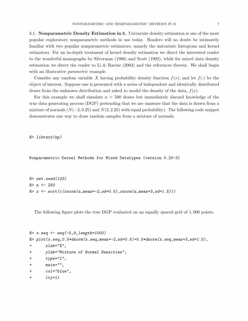
The following figure plots the true DGP evaluated on an equally spaced grid of 1, 000 points.
R> x.seq <- seq(-5,9,length=1000)
R> plot(x.seq,0.5*dnorm(x.seq,mean=-2,sd=0.5)+0.5*dnorm(x.seq,mean=3,sd=1.5),
+ xlab="X",
+ ylab="Mixture of Normal Densities",
+ type="l",
+ main="",
+ col="blue",
+ lty=1)
8 JEFFREY S. RACINE
−4 −2 0 2 4 6 8
0.0
0.1
0.2
0.3
0.4
X
Mix
ture
of N
orm
al D
ensi
ties
Suppose one naıvely presumed that the data is drawn from, say, the normal parametric family
(not a mixture thereof), then tested this assumption using the Shapiro-Wilks test. The following
code snipped demonstrates how this is done in R.
R> shapiro.test(x)
Shapiro-Wilk normality test
data: x
W = 0.87, p-value < 2.2e-16
Given that this popular parametric model is flatly rejected by this dataset, we have two choices,
namely 1) search for a more appropriate parametric model or 2) use more flexible estimators.
For what follows, we shall presume that the reader has found themselves in just such a situation.
That is, they have faithfully applied a parametric method and conducted a series of tests of model
adequacy that indicate that the parametric model is not consistent with the underlying DGP. They
then turn to more flexible methods of density estimation. Note that though we are considering

NONPARAMETRIC AND SEMIPARAMETRIC METHODS IN R 9
density estimation at the moment, it could be virtually any parametric approach that we have been
discussing, for instance, regression analysis and so forth.
If one wished to examine a histogram one could use the following code snippet,
R> hist(x,prob=TRUE,main="")
x
Den
sity
−4 −2 0 2 4 6
0.00
0.05
0.10
0.15
0.20
0.25
Of course, though consistent, the histogram suffers from a number of drawbacks hence one
might instead consider a smooth nonparametric density estimator such as the univariate Parzen
kernel estimator (Parzen (1962)). A univariate kernel estimator can be obtained using the density
command that is part of R base. This function supports a range of bandwidth methods (see ?bw.nrd
for details) and kernels (see ?density for details). The default bandwidth method is Silverman’s
’rule of thumb’ (Silverman (1986, page 48, eqn (3.31))), and for this data we obtain the following:
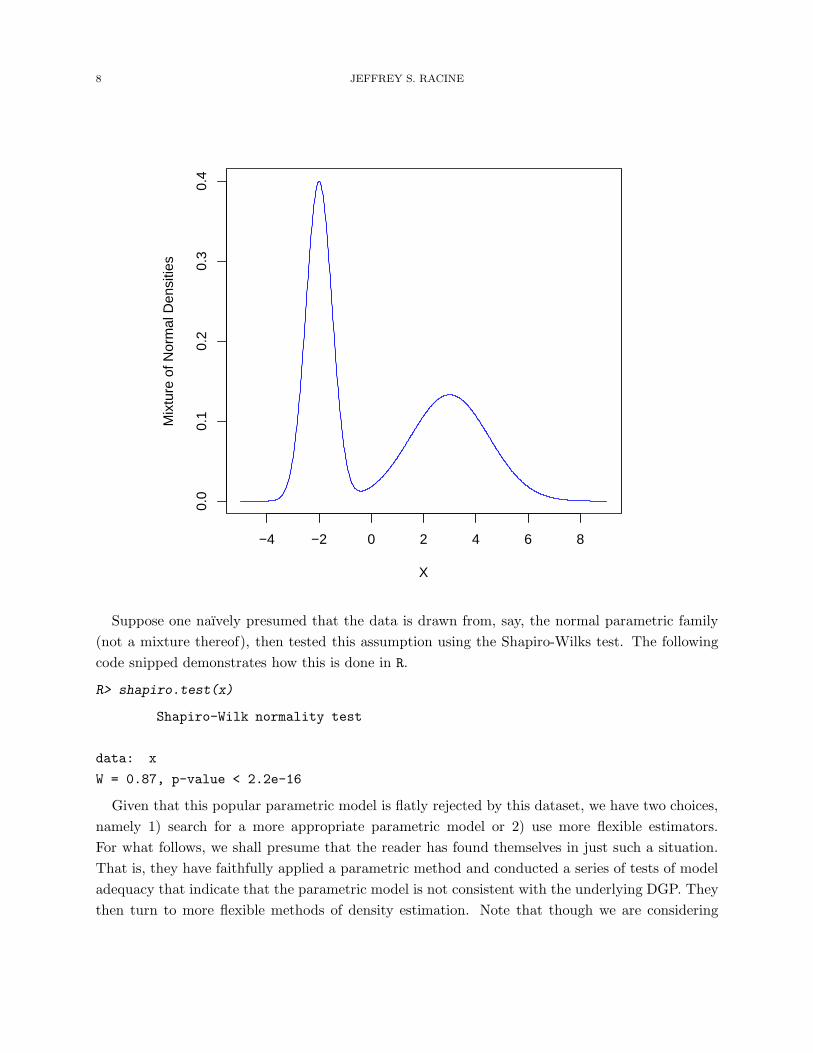
R> plot(density(x),main="")
10 JEFFREY S. RACINE
−4 −2 0 2 4 6 8
0.00
0.05
0.10
0.15
0.20
N = 500 Bandwidth = 0.7256
Den
sity
The density function in R has a number of virtues. It is extremely fast computationally speaking
as the algorithm disperses the mass of the empirical distribution function over a regular grid and
then uses the fast Fourier transform to convolve this approximation with a discretized version of
the kernel and then uses a linear approximation to evaluate the density at the specified points. If
one wishes to obtain a univariate kernel estimate for a large sample of data then this is definitely
the function of choice. However, for a bivariate (or higher dimensional) density estimate one would
require alternative R routines. The function bkd2dD in the KernSmooth package can compute a
two-dimensional density estimate as can kde2d in the MASS package and kde in the ks package
though neither package implements a data-driven two-dimensional bandwidth selector. The np
package, however, contains the function npudens that computes multivariate density estimates, is
quite flexible, and admits data-driven bandwidth selection for an arbitrary number of dimensions
and for both numeric and categorical data types. As the method does not rely on Fourier transforms
and approximations it is nowhere near as fast as the density function1, however, it is much more
1To be specific, bandwidth selection is nowhere near as fast though computing the density itself is comparable oncethe bandwidth is supplied.

NONPARAMETRIC AND SEMIPARAMETRIC METHODS IN R 11
flexible. The default method of bandwidth selection is likelihood cross-validation, and the following
code snippet demonstrates this function using the“Old Faithful”dataset. The Old Faithful Geyser is
a tourist attraction located in Yellowstone National Park. This famous dataset containing n = 272
observations consists of two variables, eruption duration (minutes) and waiting time until the next
eruption (minutes).
R> data("faithful",package="datasets")
R> fhat <- npudens(~waiting+eruptions,data=faithful)
R> plot(fhat,view="fixed",xtrim=-0.1,theta=310,phi=30,main="")
waitin
g
40
60
80
100
eruptions
2
3
4
5
Joint Density
0.00
0.01
0.02
0.03
0.04
For dimensions greater than two, one can plot“partial density surfaces”that plot one-dimensional
slices of the density holding variables not on the axes constant at their median/modes (these can
be changed by the user - see ?npplot for details). One can also plot asymptotic and bootstrapped
error surfaces, the CDF and so forth as the following code snippet reveals.
R> plot(fhat,cdf=TRUE,plot.errors.method="asymptotic",
+ view="fixed",xtrim=-0.1,theta=310,phi=30,main="")

12 JEFFREY S. RACINE
40
60
80
100
2
3
4
5
0.0
0.2
0.4
0.6
0.8
1.0
waitin
g
40
60
80
100
eruptions
2
3
4
5
Joint Distribution
0.0
0.2
0.4
0.6
0.8
1.0
40
60
80
100
2
3
4
5
0.0
0.2
0.4
0.6
0.8
1.0
3.2. Kernel Density Estimation with Numeric and Categorical Data. Suppose that we
were facing a mix of categorical and numeric data and wanted to model the joint density2 function.
When facing a mix of categorical and numeric data, traditionally researchers using kernel methods
resorted to a ‘frequency’ approach. This approach involves breaking the numeric data into subsets
according to the realizations of the categorical data (‘cells’). This of course will produce consistent
estimates. However, as the number of subsets increases, the amount of data in each cell falls leading
to a ‘sparse data’ problem. In such cases, there may be insufficient data in each subset to deliver
sensible density estimates (the estimates will be highly variable). In what follows we consider the
method of Li & Racine (2003) that is implemented in the np package via the npudens function.
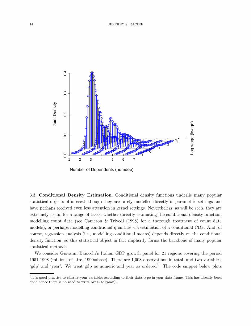
By way of example we consider Wooldridge’s (2002) ‘wage1’ dataset (n = 526), and model the
joint density of two variables, one numeric (‘lwage’) and one categorical (‘numdep’). ‘lwage’ is
the logarithm of average hourly earnings for an individual. ‘numdep’ the number of dependents
2The term ‘density’ is appropriate for distribution functions defined over mixed categorical and numeric variables. Itis the measure defined on the categorical variables in the density function that matters.
NONPARAMETRIC AND SEMIPARAMETRIC METHODS IN R 13
(0, 1, . . . ). We use likelihood cross-validation to obtain the bandwidths. Note that this is indeed
a case of ‘sparse’ data, and the traditional approach would require estimation of a nonparametric
univariate density function based upon only two observations for the last cell (c = 6).
Table 2. Summary of numdep (c = 0, 1, . . . , 6)
c nc
0 2521 1052 993 454 165 76 2
R> library(scatterplot3d)
R> data("wage1")
R> attach(wage1)
R> bw <- npudensbw(~lwage+ordered(numdep),tol=.1,ftol=.1,data=wage1)
R> numdep.seq <- sort(unique(numdep))
R> lwage.seq <- seq(min(lwage),max(lwage),length=50)
R> wage1.eval <- expand.grid(numdep=ordered(numdep.seq),lwage=lwage.seq)
R> fhat <- fitted(npudens(bws=bw,newdata=wage1.eval))
R> f <- matrix(fhat,length(unique(numdep)),50)
R> scatterplot3d(wage1.eval[,1],wage1.eval[,2],fhat,
+ ylab="Log wage (lwage)",
+ xlab="Number of Dependents (numdep)",
+ zlab="Joint Density",
+ angle=15,box=FALSE,type="h",grid=TRUE,color="blue")
R> detach(wage1)
14 JEFFREY S. RACINE
1 2 3 4 5 6 7
0.0
0.1
0.2
0.3
0.4
−1 0
1 2
3 4
Number of Dependents (numdep)
Log
wag
e (lw
age)Jo
int D
ensi
ty
3.3. Conditional Density Estimation. Conditional density functions underlie many popular
statistical objects of interest, though they are rarely modelled directly in parametric settings and
have perhaps received even less attention in kernel settings. Nevertheless, as will be seen, they are
extremely useful for a range of tasks, whether directly estimating the conditional density function,
modelling count data (see Cameron & Trivedi (1998) for a thorough treatment of count data
models), or perhaps modelling conditional quantiles via estimation of a conditional CDF. And, of
course, regression analysis (i.e., modelling conditional means) depends directly on the conditional
density function, so this statistical object in fact implicitly forms the backbone of many popular
statistical methods.
We consider Giovanni Baiocchi’s Italian GDP growth panel for 21 regions covering the period
1951-1998 (millions of Lire, 1990=base). There are 1,008 observations in total, and two variables,
‘gdp’ and ‘year’. We treat gdp as numeric and year as ordered3. The code snippet below plots
3It is good practise to classify your variables according to their data type in your data frame. This has already beendone hence there is no need to write ordered(year).
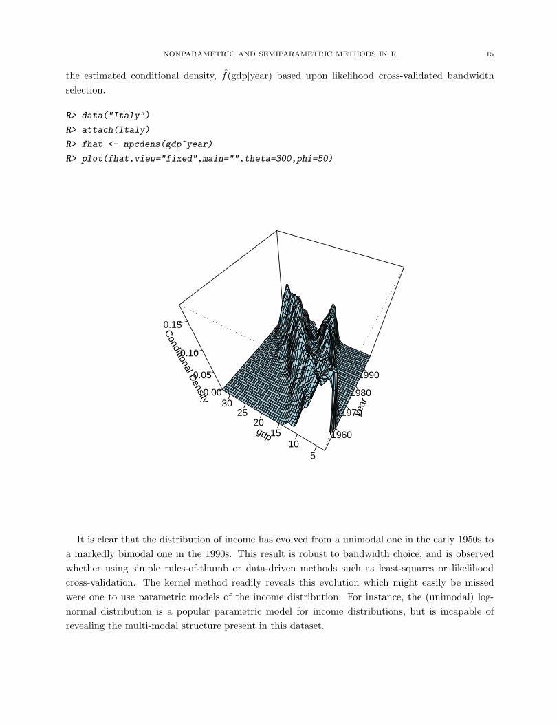
NONPARAMETRIC AND SEMIPARAMETRIC METHODS IN R 15
the estimated conditional density, f(gdp|year) based upon likelihood cross-validated bandwidth
selection.
R> data("Italy")
R> attach(Italy)
R> fhat <- npcdens(gdp~year)
R> plot(fhat,view="fixed",main="",theta=300,phi=50)
year
1960
1970
1980
1990
gdp
510
1520
2530
Conditional D
ensity0.00
0.05
0.10
0.15
It is clear that the distribution of income has evolved from a unimodal one in the early 1950s to
a markedly bimodal one in the 1990s. This result is robust to bandwidth choice, and is observed
whether using simple rules-of-thumb or data-driven methods such as least-squares or likelihood
cross-validation. The kernel method readily reveals this evolution which might easily be missed
were one to use parametric models of the income distribution. For instance, the (unimodal) log-
normal distribution is a popular parametric model for income distributions, but is incapable of
revealing the multi-modal structure present in this dataset.
16 JEFFREY S. RACINE
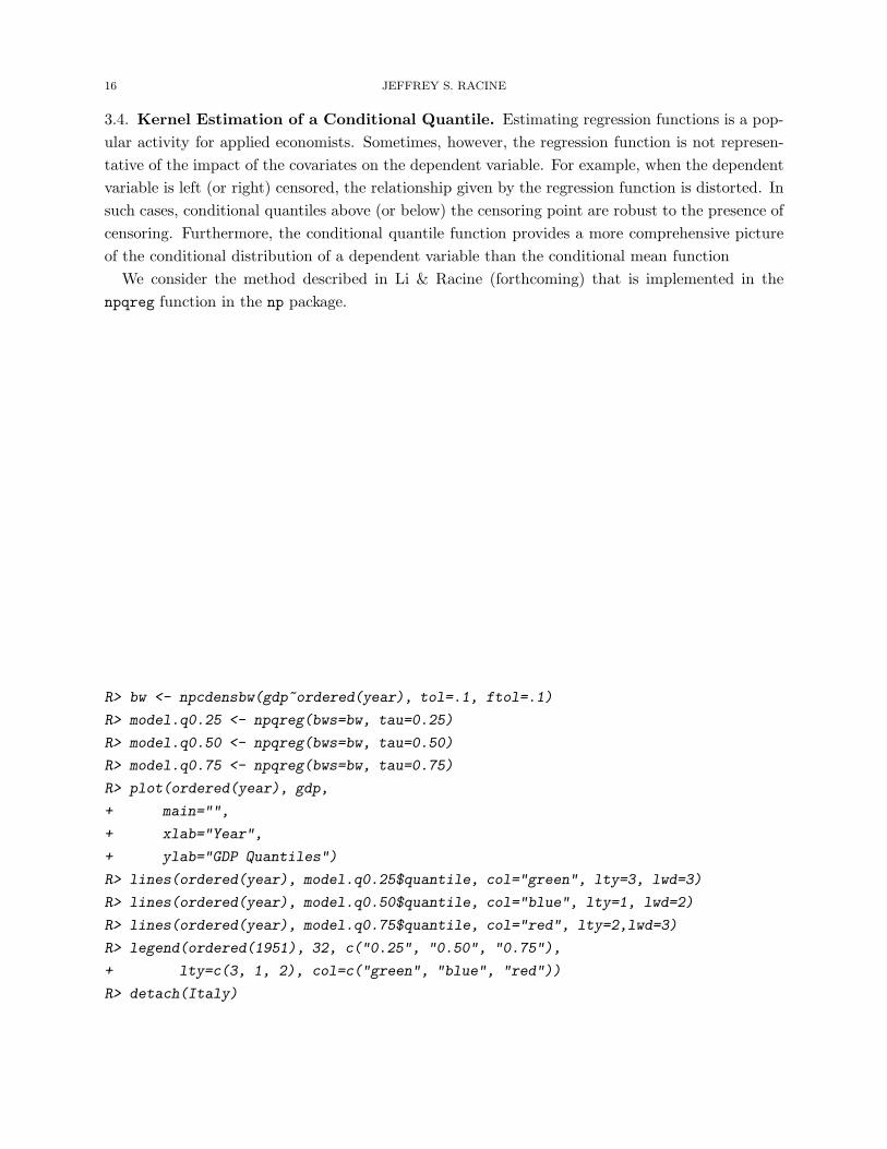
3.4. Kernel Estimation of a Conditional Quantile. Estimating regression functions is a pop-
ular activity for applied economists. Sometimes, however, the regression function is not represen-
tative of the impact of the covariates on the dependent variable. For example, when the dependent
variable is left (or right) censored, the relationship given by the regression function is distorted. In
such cases, conditional quantiles above (or below) the censoring point are robust to the presence of
censoring. Furthermore, the conditional quantile function provides a more comprehensive picture
of the conditional distribution of a dependent variable than the conditional mean function
We consider the method described in Li & Racine (forthcoming) that is implemented in the
npqreg function in the np package.
R> bw <- npcdensbw(gdp~ordered(year), tol=.1, ftol=.1)
R> model.q0.25 <- npqreg(bws=bw, tau=0.25)
R> model.q0.50 <- npqreg(bws=bw, tau=0.50)
R> model.q0.75 <- npqreg(bws=bw, tau=0.75)
R> plot(ordered(year), gdp,
+ main="",
+ xlab="Year",
+ ylab="GDP Quantiles")
R> lines(ordered(year), model.q0.25$quantile, col="green", lty=3, lwd=3)
R> lines(ordered(year), model.q0.50$quantile, col="blue", lty=1, lwd=2)
R> lines(ordered(year), model.q0.75$quantile, col="red", lty=2,lwd=3)
R> legend(ordered(1951), 32, c("0.25", "0.50", "0.75"),
+ lty=c(3, 1, 2), col=c("green", "blue", "red"))
R> detach(Italy)

NONPARAMETRIC AND SEMIPARAMETRIC METHODS IN R 17
1951 1957 1963 1969 1975 1981 1987 1993
510
1520
2530
Year
GD
P Q
uant
iles
0.250.500.75
3.5. Binary Choice and Count Data Models. We define a conditional mode by
(1) m(x) = maxy
g(y|x).
In order to estimate a conditional mode m(x), we need to model the conditional density. Let us
call m(x) the estimated conditional mode, which is given by
(2) m(x) = maxy
g(y|x),
where g(y|x) is the kernel estimator of g(y|x). By way of example, we consider modelling low
birthweights (a binary indicator) using this method.
For this example, we use data on birthweights taken from the R MASS library (Venables &
Ripley (2002)), and compute a parametric Logit model and a nonparametric conditional mode
model. We then compare their confusion matrices4 and assess their classification ability. The
4A ‘confusion matrix’ is simply a tabulation of the actual outcomes versus those predicted by a model. The diagonalelements contain correctly predicted outcomes while the off-diagonal ones contain incorrectly predicted (confused)outcomes.
18 JEFFREY S. RACINE
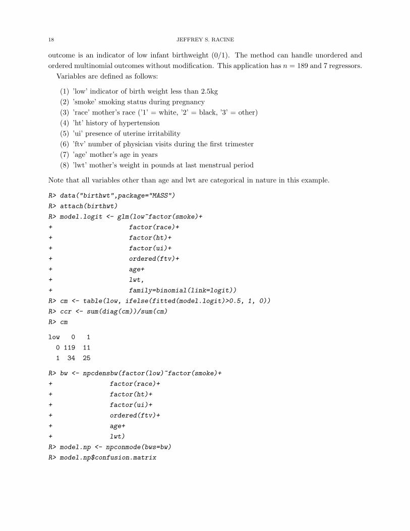
outcome is an indicator of low infant birthweight (0/1). The method can handle unordered and
ordered multinomial outcomes without modification. This application has n = 189 and 7 regressors.
Variables are defined as follows:
(1) ’low’ indicator of birth weight less than 2.5kg
(2) ’smoke’ smoking status during pregnancy
(3) ’race’ mother’s race (’1’ = white, ’2’ = black, ’3’ = other)
(4) ’ht’ history of hypertension
(5) ’ui’ presence of uterine irritability
(6) ’ftv’ number of physician visits during the first trimester
(7) ’age’ mother’s age in years
(8) ’lwt’ mother’s weight in pounds at last menstrual period
Note that all variables other than age and lwt are categorical in nature in this example.
R> data("birthwt",package="MASS")
R> attach(birthwt)
R> model.logit <- glm(low~factor(smoke)+
+ factor(race)+
+ factor(ht)+
+ factor(ui)+
+ ordered(ftv)+
+ age+
+ lwt,
+ family=binomial(link=logit))
R> cm <- table(low, ifelse(fitted(model.logit)>0.5, 1, 0))
R> ccr <- sum(diag(cm))/sum(cm)
R> cm
low 0 1
0 119 11
1 34 25
R> bw <- npcdensbw(factor(low)~factor(smoke)+
+ factor(race)+
+ factor(ht)+
+ factor(ui)+
+ ordered(ftv)+
+ age+
+ lwt)
R> model.np <- npconmode(bws=bw)
R> model.np$confusion.matrix

NONPARAMETRIC AND SEMIPARAMETRIC METHODS IN R 19
Predicted
Actual 0 1
0 127 3
1 27 32
R> detach(birthwt)
3.6. Regression. One of the most popular methods for nonparametric kernel regression was pro-
posed by Nadaraya (1965) and Watson (1964) and is known as the ‘Nadaraya-Watson’ estimator
(also known as the ‘local constant’ estimator), though the ‘local polynomial’ estimator (Fan (1992))
has emerged as a popular alternative.
For what follows, we consider an application taken from Wooldridge (2003, pg. 226) that involves
multiple regression analysis with both numeric and categorical data types.
We consider modelling an hourly wage equation for which the dependent variable is log(wage)
(lwage) while the explanatory variables include three numeric variables, namely educ (years of
education), exper (the number of years of potential experience), and tenure (the number of years
with their current employer) along with two categorical variables, female (‘Female’/‘Male’) and
married (‘Married’/‘Notmarried’). For this example there are n = 526 observations. We use
Hurvich, Simonoff & Tsai’s (1998) AICc approach for bandwidth selection.
R> attach(wage1)
R> #bw.all <- npregbw(formula=lwage~factor(female)+
R> # factor(married)+
R> # educ+
R> # exper+
R> # tenure,
R> # regtype="ll",
R> # bwmethod="cv.aic",
R> # data=wage1)
R>
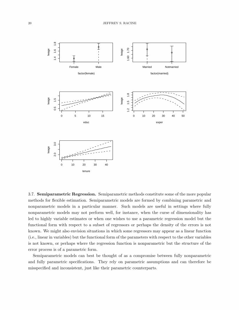
R> model.np <- npreg(bws=bw.all)
R> plot(model.np,
+ plot.errors.method="bootstrap",
+ plot.errors.boot.num=100,
+ plot.errors.type="quantiles",
+ plot.errors.style="band",
+ common.scale=FALSE)
R> detach(wage1)
20 JEFFREY S. RACINE
Female Male
1.4
1.6
1.8
factor(female)
lwag
e
Married Notmarried
1.60
1.70
factor(married)
lwag
e
0 5 10 15
0.5
1.5
educ
lwag
e
0 10 20 30 40 50
1.2
1.5
1.8
exper lw
age
0 10 20 30 40
2.0
3.0
tenure
lwag
e
3.7. Semiparametric Regression. Semiparametric methods constitute some of the more popular
methods for flexible estimation. Semiparametric models are formed by combining parametric and
nonparametric models in a particular manner. Such models are useful in settings where fully
nonparametric models may not perform well, for instance, when the curse of dimensionality has
led to highly variable estimates or when one wishes to use a parametric regression model but the
functional form with respect to a subset of regressors or perhaps the density of the errors is not
known. We might also envision situations in which some regressors may appear as a linear function
(i.e., linear in variables) but the functional form of the parameters with respect to the other variables
is not known, or perhaps where the regression function is nonparametric but the structure of the
error process is of a parametric form.
Semiparametric models can best be thought of as a compromise between fully nonparametric
and fully parametric specifications. They rely on parametric assumptions and can therefore be
misspecified and inconsistent, just like their parametric counterparts.
NONPARAMETRIC AND SEMIPARAMETRIC METHODS IN R 21
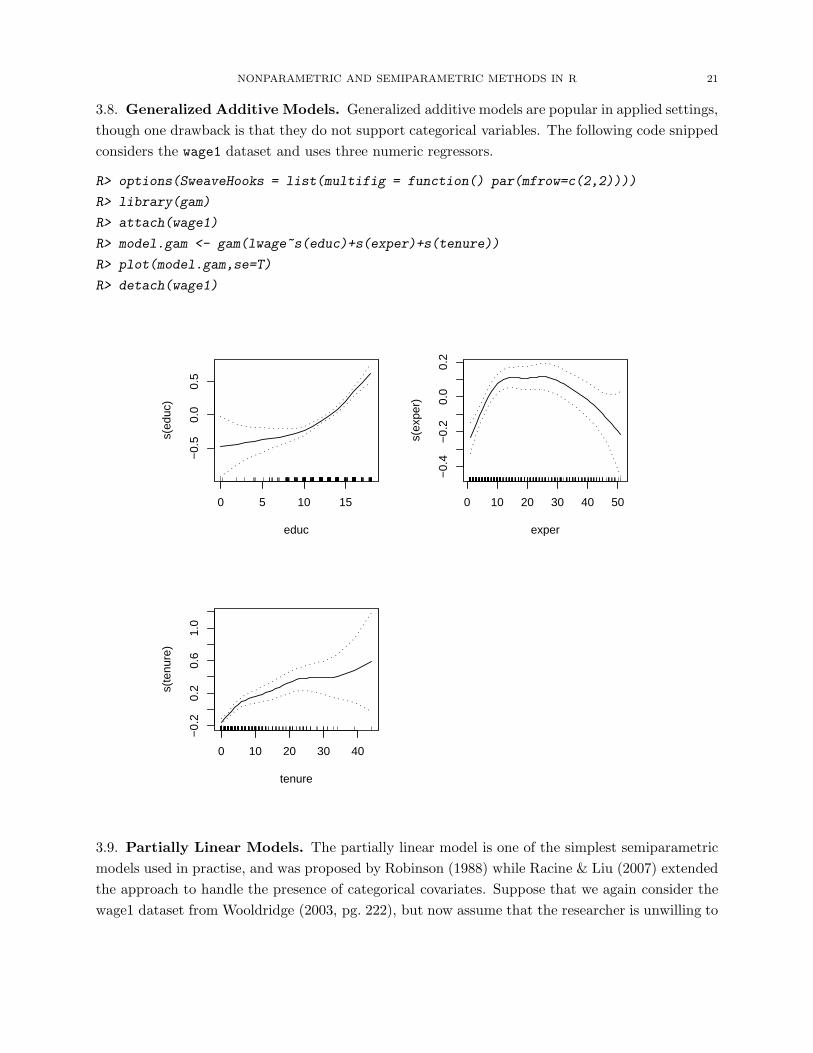
3.8. Generalized Additive Models. Generalized additive models are popular in applied settings,
though one drawback is that they do not support categorical variables. The following code snipped
considers the wage1 dataset and uses three numeric regressors.
R> options(SweaveHooks = list(multifig = function() par(mfrow=c(2,2))))
R> library(gam)
R> attach(wage1)
R> model.gam <- gam(lwage~s(educ)+s(exper)+s(tenure))
R> plot(model.gam,se=T)
R> detach(wage1)
0 5 10 15
−0.
50.
00.
5
educ
s(ed
uc)
0 10 20 30 40 50
−0.
4−
0.2
0.0
0.2
exper
s(ex
per)
0 10 20 30 40
−0.
20.
20.
61.
0
tenure
s(te
nure
)
3.9. Partially Linear Models. The partially linear model is one of the simplest semiparametric
models used in practise, and was proposed by Robinson (1988) while Racine & Liu (2007) extended
the approach to handle the presence of categorical covariates. Suppose that we again consider the
wage1 dataset from Wooldridge (2003, pg. 222), but now assume that the researcher is unwilling to
22 JEFFREY S. RACINE
presume the nature of the relationship between exper and lwage, hence relegates exper to the non-
parametric part of a semiparametric partially linear model. The following code snipped considers
a popular parametric specification followed by a partially linear one.
R> model.lm <- lm(formula=lwage~factor(female)+
+ factor(married)+
+ educ+
+ tenure+
+ exper+
+ I(exper^2),
+ data=wage1)
R> summary(model.lm)
Call:
lm(formula = lwage ~ factor(female) + factor(married) + educ +
tenure + exper + I(exper^2), data = wage1)
Residuals:
Min 1Q Median 3Q Max
-1.8185 -0.2568 -0.0253 0.2475 1.1815
Coefficients:
Estimate Std. Error t value Pr(>|t|)
(Intercept) 0.181161 0.107075 1.69 0.091 .
factor(female)Male 0.291130 0.036283 8.02 6.9e-15 ***
factor(married)Notmarried -0.056449 0.040926 -1.38 0.168
educ 0.079832 0.006827 11.69 < 2e-16 ***
tenure 0.016074 0.002880 5.58 3.9e-08 ***
exper 0.030100 0.005193 5.80 1.2e-08 ***
I(exper^2) -0.000601 0.000110 -5.47 7.0e-08 ***
---
Signif. codes: 0 '***' 0.001 '**' 0.01 '*' 0.05 '.' 0.1 ' ' 1
Residual standard error: 0.401 on 519 degrees of freedom
Multiple R-squared: 0.436, Adjusted R-squared: 0.43
F-statistic: 66.9 on 6 and 519 DF, p-value: <2e-16
R> bw <- npplregbw(formula=lwage~factor(female)+
+ factor(married)+
+ educ+
+ tenure|exper,
NONPARAMETRIC AND SEMIPARAMETRIC METHODS IN R 23
+ data=wage1)
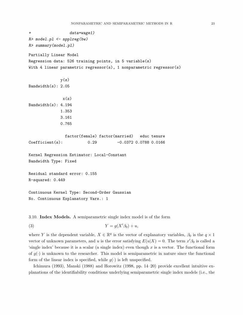
R> model.pl <- npplreg(bw)
R> summary(model.pl)
Partially Linear Model
Regression data: 526 training points, in 5 variable(s)
With 4 linear parametric regressor(s), 1 nonparametric regressor(s)
y(z)
Bandwidth(s): 2.05
x(z)
Bandwidth(s): 4.194
1.353
3.161
0.765
factor(female) factor(married) educ tenure
Coefficient(s): 0.29 -0.0372 0.0788 0.0166
Kernel Regression Estimator: Local-Constant
Bandwidth Type: Fixed
Residual standard error: 0.155
R-squared: 0.449
Continuous Kernel Type: Second-Order Gaussian
No. Continuous Explanatory Vars.: 1
3.10. Index Models. A semiparametric single index model is of the form
(3) Y = g(X ′β0) + u,
where Y is the dependent variable, X ∈ Rq is the vector of explanatory variables, β0 is the q × 1
vector of unknown parameters, and u is the error satisfying E(u|X) = 0. The term x′β0 is called a
‘single index’ because it is a scalar (a single index) even though x is a vector. The functional form
of g(·) is unknown to the researcher. This model is semiparametric in nature since the functional
form of the linear index is specified, while g(·) is left unspecified.
Ichimura (1993), Manski (1988) and Horowitz (1998, pp. 14–20) provide excellent intuitive ex-
planations of the identifiability conditions underlying semiparametric single index models (i.e., the
24 JEFFREY S. RACINE
set of conditions under which the unknown parameter vector β0 and the unknown function g(·) can
be sensibly estimated), and we direct the reader to these references for details.
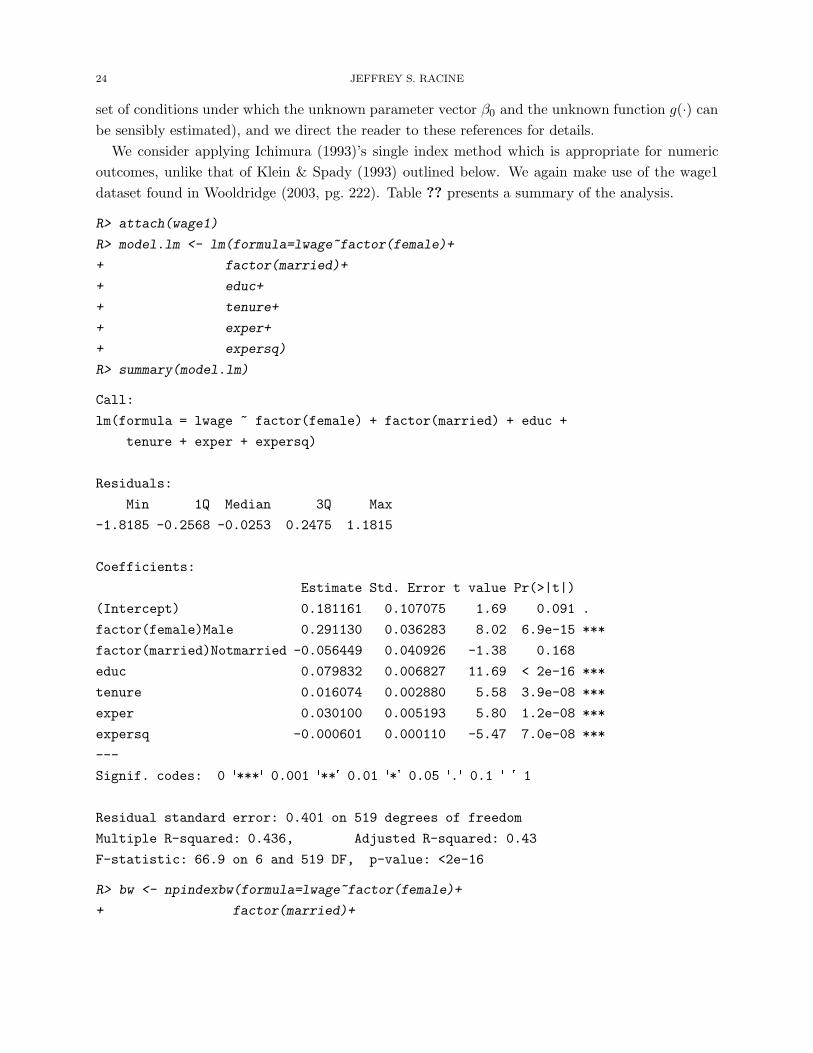
We consider applying Ichimura (1993)’s single index method which is appropriate for numeric
outcomes, unlike that of Klein & Spady (1993) outlined below. We again make use of the wage1
dataset found in Wooldridge (2003, pg. 222). Table ?? presents a summary of the analysis.
R> attach(wage1)
R> model.lm <- lm(formula=lwage~factor(female)+
+ factor(married)+
+ educ+
+ tenure+
+ exper+
+ expersq)
R> summary(model.lm)
Call:
lm(formula = lwage ~ factor(female) + factor(married) + educ +
tenure + exper + expersq)
Residuals:
Min 1Q Median 3Q Max
-1.8185 -0.2568 -0.0253 0.2475 1.1815
Coefficients:
Estimate Std. Error t value Pr(>|t|)
(Intercept) 0.181161 0.107075 1.69 0.091 .
factor(female)Male 0.291130 0.036283 8.02 6.9e-15 ***
factor(married)Notmarried -0.056449 0.040926 -1.38 0.168
educ 0.079832 0.006827 11.69 < 2e-16 ***
tenure 0.016074 0.002880 5.58 3.9e-08 ***
exper 0.030100 0.005193 5.80 1.2e-08 ***
expersq -0.000601 0.000110 -5.47 7.0e-08 ***
---
Signif. codes: 0 '***' 0.001 '**' 0.01 '*' 0.05 '.' 0.1 ' ' 1
Residual standard error: 0.401 on 519 degrees of freedom
Multiple R-squared: 0.436, Adjusted R-squared: 0.43
F-statistic: 66.9 on 6 and 519 DF, p-value: <2e-16
R> bw <- npindexbw(formula=lwage~factor(female)+
+ factor(married)+
NONPARAMETRIC AND SEMIPARAMETRIC METHODS IN R 25
+ educ+
+ exper+
+ expersq+
+ tenure,
+ data=wage1)
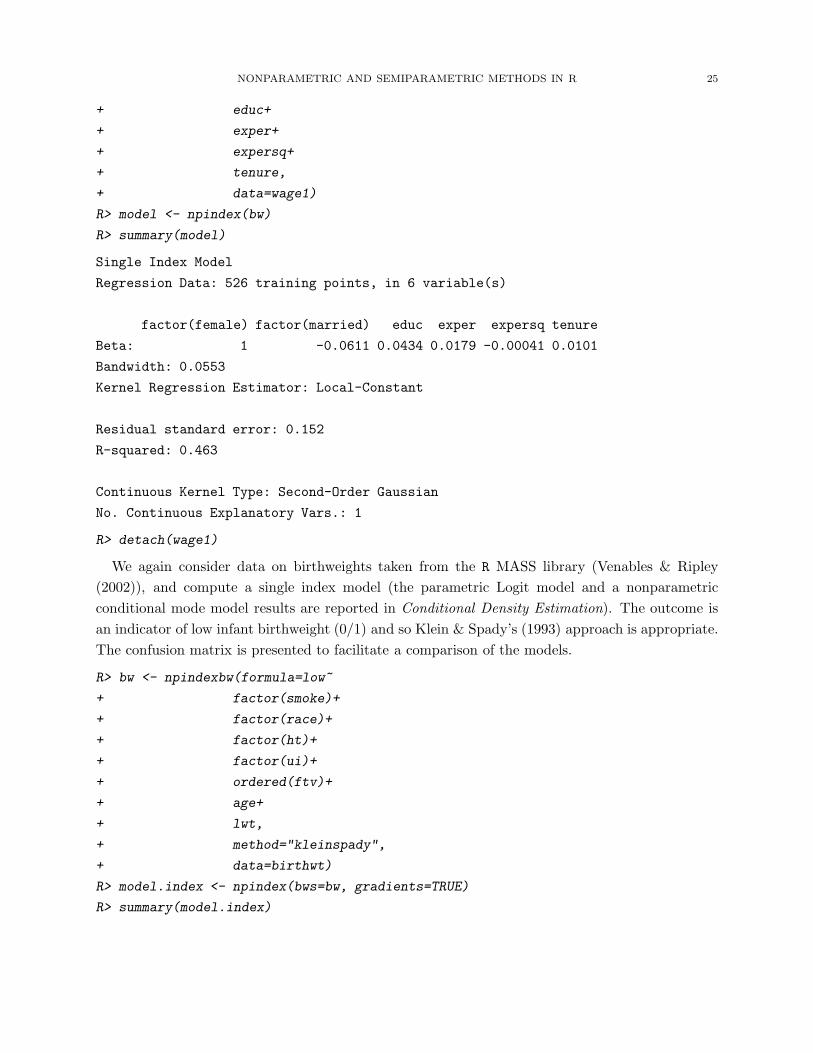
R> model <- npindex(bw)
R> summary(model)
Single Index Model
Regression Data: 526 training points, in 6 variable(s)
factor(female) factor(married) educ exper expersq tenure
Beta: 1 -0.0611 0.0434 0.0179 -0.00041 0.0101
Bandwidth: 0.0553
Kernel Regression Estimator: Local-Constant
Residual standard error: 0.152
R-squared: 0.463
Continuous Kernel Type: Second-Order Gaussian
No. Continuous Explanatory Vars.: 1
R> detach(wage1)
We again consider data on birthweights taken from the R MASS library (Venables & Ripley
(2002)), and compute a single index model (the parametric Logit model and a nonparametric
conditional mode model results are reported in Conditional Density Estimation). The outcome is
an indicator of low infant birthweight (0/1) and so Klein & Spady’s (1993) approach is appropriate.
The confusion matrix is presented to facilitate a comparison of the models.
R> bw <- npindexbw(formula=low~
+ factor(smoke)+
+ factor(race)+
+ factor(ht)+
+ factor(ui)+
+ ordered(ftv)+
+ age+
+ lwt,
+ method="kleinspady",
+ data=birthwt)
R> model.index <- npindex(bws=bw, gradients=TRUE)
R> summary(model.index)
26 JEFFREY S. RACINE
Single Index Model
Regression Data: 189 training points, in 7 variable(s)
factor(smoke) factor(race) factor(ht) factor(ui) ordered(ftv) age
Beta: 1 0.0508 0.363 0.184 -0.0505 -0.0158
lwt
Beta: -0.00145
Bandwidth: 0.0159
Kernel Regression Estimator: Local-Constant
Confusion Matrix
Predicted
Actual 0 1
0 119 11
1 22 37
Overall Correct Classification Ratio: 0.825
Correct Classification Ratio By Outcome:
0 1
0.915 0.627
McFadden-Puig-Kerschner performance measure: 0.808
Continuous Kernel Type: Second-Order Gaussian
No. Continuous Explanatory Vars.: 1
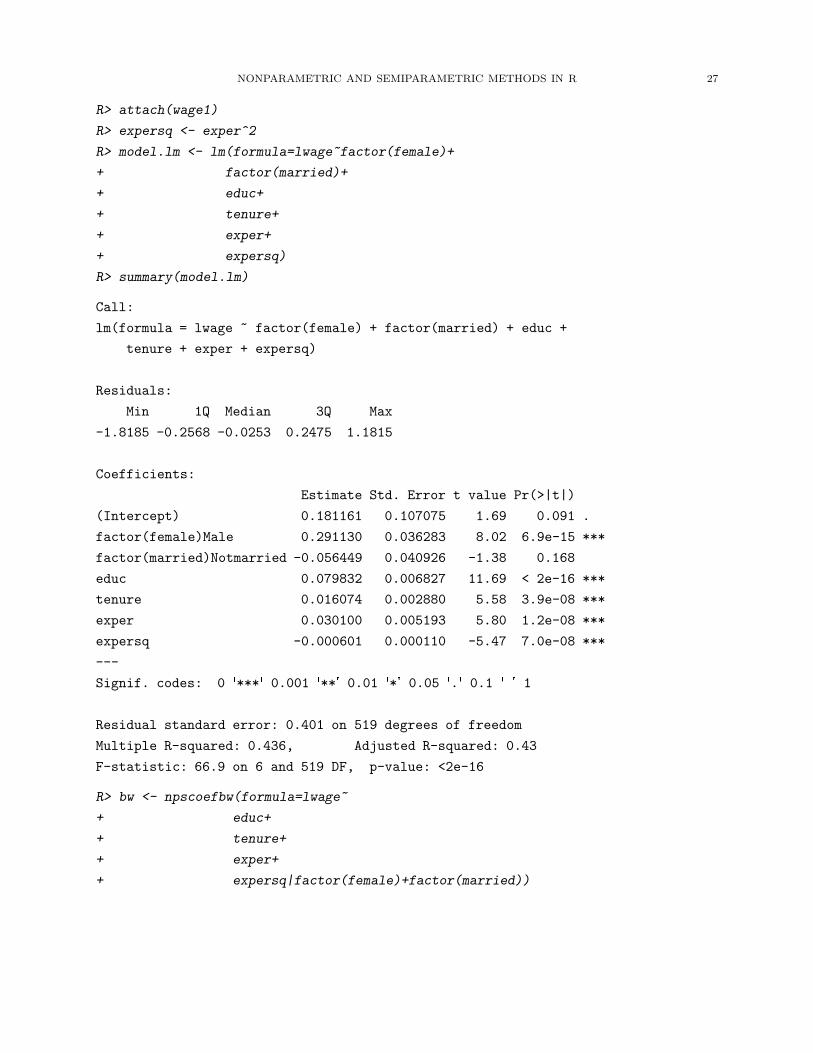
3.11. Smooth Coefficient (Varying Coefficient) Models. The smooth coefficient model is
given by
Yi = α(Zi) + X ′
iβ(Zi) + ui
= (1 + X ′
i)
(
α(Zi)
β(Zi)
)
+ ui
= W ′
iγ(Zi) + ui
(4)
where Xi is a k × 1 vector and where β(z) is a vector of unspecified smooth functions of z.
Suppose that we once again consider the wage1 dataset from Wooldridge (2003, pg. 222), but
now assume that the researcher is unwilling to presume that the coefficients associated with the
numeric variables do not vary with respect to the categorical variables female and married. The
following code snipped presents a summary from the linear and smooth coefficient specification.
NONPARAMETRIC AND SEMIPARAMETRIC METHODS IN R 27
R> attach(wage1)
R> expersq <- exper^2
R> model.lm <- lm(formula=lwage~factor(female)+
+ factor(married)+
+ educ+
+ tenure+
+ exper+
+ expersq)
R> summary(model.lm)
Call:
lm(formula = lwage ~ factor(female) + factor(married) + educ +
tenure + exper + expersq)
Residuals:
Min 1Q Median 3Q Max
-1.8185 -0.2568 -0.0253 0.2475 1.1815
Coefficients:
Estimate Std. Error t value Pr(>|t|)
(Intercept) 0.181161 0.107075 1.69 0.091 .
factor(female)Male 0.291130 0.036283 8.02 6.9e-15 ***
factor(married)Notmarried -0.056449 0.040926 -1.38 0.168
educ 0.079832 0.006827 11.69 < 2e-16 ***
tenure 0.016074 0.002880 5.58 3.9e-08 ***
exper 0.030100 0.005193 5.80 1.2e-08 ***
expersq -0.000601 0.000110 -5.47 7.0e-08 ***
---
Signif. codes: 0 '***' 0.001 '**' 0.01 '*' 0.05 '.' 0.1 ' ' 1
Residual standard error: 0.401 on 519 degrees of freedom
Multiple R-squared: 0.436, Adjusted R-squared: 0.43
F-statistic: 66.9 on 6 and 519 DF, p-value: <2e-16
R> bw <- npscoefbw(formula=lwage~
+ educ+
+ tenure+
+ exper+
+ expersq|factor(female)+factor(married))
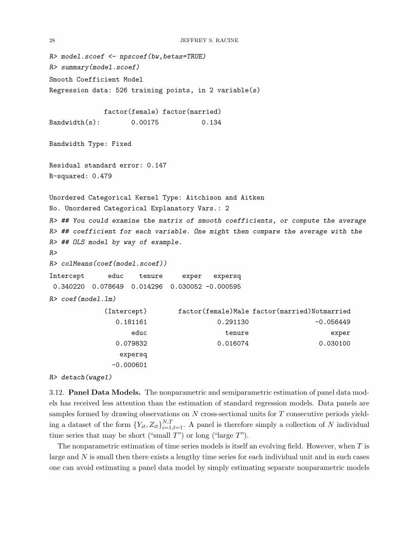
28 JEFFREY S. RACINE
R> model.scoef <- npscoef(bw,betas=TRUE)
R> summary(model.scoef)
Smooth Coefficient Model
Regression data: 526 training points, in 2 variable(s)
factor(female) factor(married)
Bandwidth(s): 0.00175 0.134
Bandwidth Type: Fixed
Residual standard error: 0.147
R-squared: 0.479
Unordered Categorical Kernel Type: Aitchison and Aitken
No. Unordered Categorical Explanatory Vars.: 2
R> ## You could examine the matrix of smooth coefficients, or compute the average
R> ## coefficient for each variable. One might then compare the average with the
R> ## OLS model by way of example.
R>
R> colMeans(coef(model.scoef))
Intercept educ tenure exper expersq
0.340220 0.078649 0.014296 0.030052 -0.000595
R> coef(model.lm)
(Intercept) factor(female)Male factor(married)Notmarried
0.181161 0.291130 -0.056449
educ tenure exper
0.079832 0.016074 0.030100
expersq
-0.000601
R> detach(wage1)
3.12. Panel Data Models. The nonparametric and semiparametric estimation of panel data mod-
els has received less attention than the estimation of standard regression models. Data panels are
samples formed by drawing observations on N cross-sectional units for T consecutive periods yield-
ing a dataset of the form {Yit, Zit}N,Ti=1,t=1
. A panel is therefore simply a collection of N individual
time series that may be short (“small T”) or long (“large T”).
The nonparametric estimation of time series models is itself an evolving field. However, when T is
large and N is small then there exists a lengthy time series for each individual unit and in such cases
one can avoid estimating a panel data model by simply estimating separate nonparametric models
NONPARAMETRIC AND SEMIPARAMETRIC METHODS IN R 29
for each individual unit using the T individual time series available for each. If this situation applies,
we direct the interested reader to Li & Racine (2007a, Chapter 18) for pointers to the literature on
nonparametric methods for time series data.
When contemplating the nonparametric estimation of panel data models, one issue that immedi-
ately arises is that the standard (parametric) approaches that are often used for panel data models
(such as first-differencing to remove the presence of so-called ‘fixed effects’) are no longer valid
unless one is willing to presume additively separable effects, which for many defeats the purpose of
using nonparametric methods in the first place.
A variety of approaches have been proposed in the literature, including Wang (2003), who pro-
posed a novel method for estimating nonparametric panel data models that utilizes the information
contained in the covariance structure of the model’s disturbances, Wang, Carroll & Lin (2005) who
proposed a partially linear model with random effects, and Henderson, Carroll & Li (2006) who con-
sider profile likelihood methods for nonparametric estimation of additive fixed effect models which
are removed via first differencing. In what follows, we consider direct nonparametric estimation of
fixed effects models.
Consider the following nonparametric fixed effects panel data regression model,
Yit = g(Xit) + uit, i = 1, 2 . . . , N, t = 1, 2, . . . , T,
where g(·) is an unknown smooth function, Xit = (Xit,1, . . . ,Xit,q) is of dimension q, all other
variables are scalars, and E(uit|Xi1, . . . ,XiT ) = 0.
We say that panel data is ‘poolable’ if one can ‘pool’ the data, by in effect, ignoring the time
series dimension, that is, by summing over both i and t without regard to the time dimension
thereby effectively putting all data into the same pool then directly applying the methods in, say,
Regression. Of course, if the data is not poolable this would obviously not be a wise choice.
However, to allow for the possibility that the data is in fact potentially poolable, one can introduce
an unordered categorical variable, say δi = i for i = 1, 2, . . . , N , and estimate E(Yit|Zit, δi) =
g(Zit, δi) nonparametrically using the mixed categorical and numeric kernel approach introduced
in Density and Probability Function Estimation. Letting λ denote the cross-validated smoothing
parameter associated with δi, then if λ = 1, one gets g(Zit, δi) = g(Zit) and the data is thereby
pooled in the resulting estimate of g(·). If, on the other hand, λ = 0 (or is close to 0), then this
effectively estimates each gi(·) using only the time series for the ith individual unit. Finally, if
0 < λ < 1, one might interpret this as a case in which the data is partially poolable.
We consider a panel of annual observations for six U.S. airlines for the fifteen year period 1970
to 1984 taken from the Ecdat R package (Croissant (2006)) as detailed in Greene (2003, Table F7.1,
page 949)). The variables in the panel are airline (‘airline’), year (‘year’), the logarithm of total
cost in $1,000 (‘lcost’), the logarithm of an output index in revenue passenger miles (‘loutput’), the
logarithm of the price of fuel (‘lpf’), and load factor, i.e., the average capacity utilization of the
fleet (‘lf’). We treat ‘airline’ as an ordered factor and ‘year’ as an ordered factor and use a local
linear estimator with Hurvich et al.’s (1998) AICc approach.
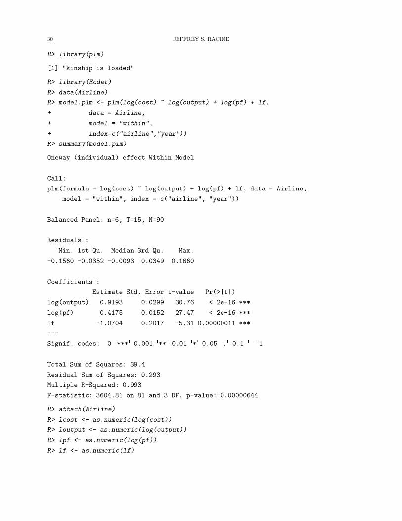
30 JEFFREY S. RACINE
R> library(plm)
[1] "kinship is loaded"
R> library(Ecdat)
R> data(Airline)
R> model.plm <- plm(log(cost) ~ log(output) + log(pf) + lf,
+ data = Airline,
+ model = "within",
+ index=c("airline","year"))
R> summary(model.plm)
Oneway (individual) effect Within Model
Call:
plm(formula = log(cost) ~ log(output) + log(pf) + lf, data = Airline,
model = "within", index = c("airline", "year"))
Balanced Panel: n=6, T=15, N=90
Residuals :
Min. 1st Qu. Median 3rd Qu. Max.
-0.1560 -0.0352 -0.0093 0.0349 0.1660
Coefficients :
Estimate Std. Error t-value Pr(>|t|)
log(output) 0.9193 0.0299 30.76 < 2e-16 ***
log(pf) 0.4175 0.0152 27.47 < 2e-16 ***
lf -1.0704 0.2017 -5.31 0.00000011 ***
---
Signif. codes: 0 '***' 0.001 '**' 0.01 '*' 0.05 '.' 0.1 ' ' 1
Total Sum of Squares: 39.4
Residual Sum of Squares: 0.293
Multiple R-Squared: 0.993
F-statistic: 3604.81 on 81 and 3 DF, p-value: 0.00000644
R> attach(Airline)
R> lcost <- as.numeric(log(cost))
R> loutput <- as.numeric(log(output))
R> lpf <- as.numeric(log(pf))
R> lf <- as.numeric(lf)
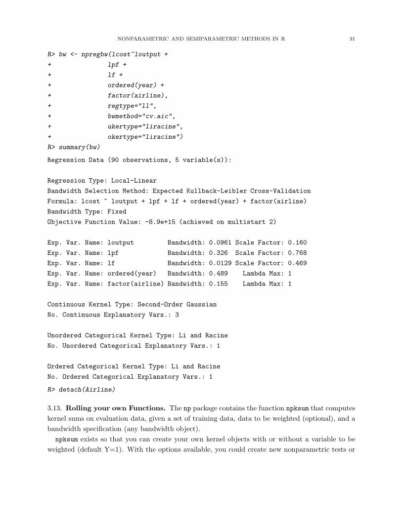
NONPARAMETRIC AND SEMIPARAMETRIC METHODS IN R 31
R> bw <- npregbw(lcost~loutput +
+ lpf +
+ lf +
+ ordered(year) +
+ factor(airline),
+ regtype="ll",
+ bwmethod="cv.aic",
+ ukertype="liracine",
+ okertype="liracine")
R> summary(bw)
Regression Data (90 observations, 5 variable(s)):
Regression Type: Local-Linear
Bandwidth Selection Method: Expected Kullback-Leibler Cross-Validation
Formula: lcost ~ loutput + lpf + lf + ordered(year) + factor(airline)
Bandwidth Type: Fixed
Objective Function Value: -8.9e+15 (achieved on multistart 2)
Exp. Var. Name: loutput Bandwidth: 0.0961 Scale Factor: 0.160
Exp. Var. Name: lpf Bandwidth: 0.326 Scale Factor: 0.768
Exp. Var. Name: lf Bandwidth: 0.0129 Scale Factor: 0.469
Exp. Var. Name: ordered(year) Bandwidth: 0.489 Lambda Max: 1
Exp. Var. Name: factor(airline) Bandwidth: 0.155 Lambda Max: 1
Continuous Kernel Type: Second-Order Gaussian
No. Continuous Explanatory Vars.: 3
Unordered Categorical Kernel Type: Li and Racine
No. Unordered Categorical Explanatory Vars.: 1
Ordered Categorical Kernel Type: Li and Racine
No. Ordered Categorical Explanatory Vars.: 1
R> detach(Airline)
3.13. Rolling your own Functions. The np package contains the function npksum that computes
kernel sums on evaluation data, given a set of training data, data to be weighted (optional), and a
bandwidth specification (any bandwidth object).
npksum exists so that you can create your own kernel objects with or without a variable to be
weighted (default Y=1). With the options available, you could create new nonparametric tests or
32 JEFFREY S. RACINE
even new kernel estimators. The convolution kernel option would allow you to create, say, the least
squares cross-validation function for kernel density estimation.
npksum uses highly-optimized C code that strives to minimize its ’memory footprint’, while there
is low overhead involved when using repeated calls to this function (see, by way of illustration, the
example below that conducts leave-one-out cross-validation for a local constant regression estimator
via calls to the ’R’ function ’nlm’, and compares this to the ’npregbw’ function).
npksum implements a variety of methods for computing multivariate kernel sums (p-variate)
defined over a set of possibly numeric and/or categorical (unordered, ordered) data. The approach
is based on Li and Racine (2003) who employ ’generalized product kernels’ that admit a mix of
numeric and categorical data types.
Three classes of kernel estimators for the numeric data types are available: fixed, adaptive
nearest-neighbor, and generalized nearest-neighbor. Adaptive nearest-neighbor bandwidths change
with each sample realization in the set, x[i], when estimating the kernel sum at the point x. Gen-
eralized nearest-neighbor bandwidths change with the point at which the sum is computed, x.
Fixed bandwidths are constant over the support of x. npksum computes∑
j W ′
jYjK(Xj), where
Aj represents a row vector extracted from A. That is, it computes the kernel weighted sum of the
outer product of the rows of W and Y . In the examples from ?npksum, the uses of such sums are
illustrated.
npksum may be invoked either with a formula-like symbolic description of variables on which
the sum is to be performed or through a simpler interface whereby data is passed directly to the
function via the ’txdat’ and ’tydat’ parameters. Use of these two interfaces is mutually exclusive.
Data contained in the data frame ’txdat’ (and also ’exdat’) may be a mix of numeric (default),
unordered categorical (to be specified in the data frame ’txdat’ using the ’factor’ command), and
ordered categorical (to be specified in the data frame ’txdat’ using the ’ordered’ command). Data
can be entered in an arbitrary order and data types will be detected automatically by the routine
(see ’np’ for details).
Data for which bandwidths are to be estimated may be specified symbolically. A typical descrip-
tion has the form ’dependent data explanatory data’, where ’dependent data’ and ’explanatory
data’ are both series of variables specified by name, separated by the separation character ’+’. For
example, y1 ~ x1 + x2 specifies that y1 is to be kernel-weighted by x1 and x2 throughout the
sum. See below for further examples.
A variety of kernels may be specified by the user. Kernels implemented for numeric data types
include the second, fourth, sixth, and eighth order Gaussian and Epanechnikov kernels, and the
uniform kernel. Unordered categorical data types use a variation on Aitchison and Aitken’s (1976)
kernel, while ordered data types use a variation of the Wang and van Ryzin (1981) kernel (see ’np’
for details).
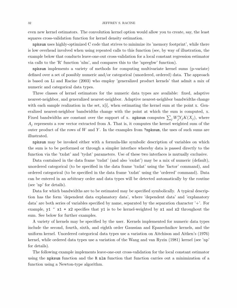
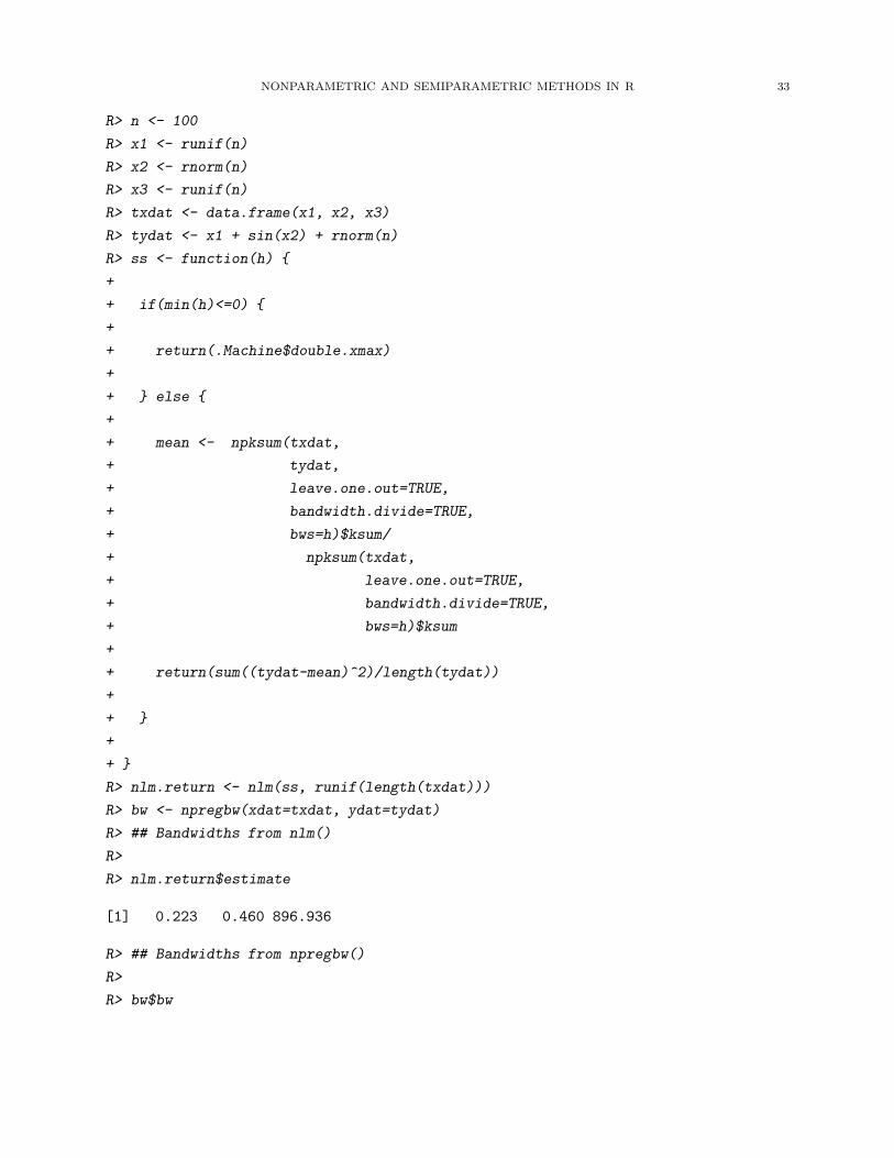
The following example implements leave-one-out cross-validation for the local constant estimator
using the npksum function and the R nlm function that function carries out a minimization of a
function using a Newton-type algorithm.
NONPARAMETRIC AND SEMIPARAMETRIC METHODS IN R 33
R> n <- 100
R> x1 <- runif(n)
R> x2 <- rnorm(n)
R> x3 <- runif(n)
R> txdat <- data.frame(x1, x2, x3)
R> tydat <- x1 + sin(x2) + rnorm(n)
R> ss <- function(h) {
+
+ if(min(h)<=0) {
+
+ return(.Machine$double.xmax)
+
+ } else {
+
+ mean <- npksum(txdat,
+ tydat,
+ leave.one.out=TRUE,
+ bandwidth.divide=TRUE,
+ bws=h)$ksum/
+ npksum(txdat,
+ leave.one.out=TRUE,
+ bandwidth.divide=TRUE,
+ bws=h)$ksum
+
+ return(sum((tydat-mean)^2)/length(tydat))
+
+ }
+
+ }
R> nlm.return <- nlm(ss, runif(length(txdat)))
R> bw <- npregbw(xdat=txdat, ydat=tydat)
R> ## Bandwidths from nlm()
R>
R> nlm.return$estimate
[1] 0.223 0.460 896.936
R> ## Bandwidths from npregbw()
R>
R> bw$bw
34 JEFFREY S. RACINE
[1] 0.223 0.460 1602195.268
R> ## Function value (minimum) from nlm()
R>
R> nlm.return$minimum
[1] 0.953
R> ## Function value (minimum) from npregbw()
R>
R> bw$fval
[1] 0.953
4. Summary
The R environment for statistical computing and graphics (R Development Core Team (2008))
offers practitioners a rich set of statistical methods ranging from random number generation and op-
timization methods through regression, panel data, and time series methods, by way of illustration.
The standard R distribution (‘base R) comes preloaded with a rich variety of functionality useful for
applied econometricians. This functionality is enhanced by user supplied packages made available
via R servers that are mirrored around the world. We hope that this chapter will encourage users
to pursue the R environment should they wish to adopt nonparametric or semiparametric methods,
and we wholeheartedly encourage those working in the field to strongly consider implementing their
methods in the R environment thereby making their work accessible to the widest possible audience
via an open collaborative forum.
References
Cameron, A. C. & Trivedi, P. K. (1998), Regression Analysis of Count Data, Cambridge University Press, New York.
Chambers, J. M. & Hastie, T. (1991), Statistical models in S, London: Chapman & Hall.
Cleveland, W. S., Grosse, E. & Shyu, W. M. (1992), Local regression models, in J. M. Chambers & T. J. Hastie, eds,
‘Statistical Models in S’, Wadsworth and Brooks/Cole, Pacific Grove, CA, chapter 8.
Croissant, Y. (2006), Ecdat: Data sets for econometrics. R package version 0.1-5.
URL: http://www.r-project.org
Fan, J. (1992), ‘Design-adaptive nonparametric regression’, Journal of the American Statistical Association 87, 998–
1004.
Greene, W. H. (2003), Econometric Analysis, fifth edn, Prentice Hall, Upper Saddle River, NJ.
Hall, P., Racine, J. S. & Li, Q. (2004), ‘Cross-validation and the estimation of conditional probability densities’,
Journal of the American Statistical Association 99(468), 1015–1026.
Hastie, T. & Tibshirani, R. (1990), Generalized additive models, Chapman and Hall, London.
Hayfield, T. & Racine, J. S. (2008), ‘Nonparametric econometrics: The np package’, Journal of Statistical Software
27(5).
URL: http://www.jstatsoft.org/v27/i05/
Henderson, D., Carroll, R. J. & Li, Q. (2006), Nonparametric estimation and testing of fixed effects panel data models,
Unpublished manuscript, Texas A & M University.
Horowitz, J. L. (1998), Semiparametric Methods in Econometrics, Springer-Verlag, New York.
NONPARAMETRIC AND SEMIPARAMETRIC METHODS IN R 35
Hsiao, C., Li, Q. & Racine, J. S. (2007), ‘A consistent model specification test with mixed categorical and continuous
data’, Journal of Econometrics 140, 802–826.
Hurvich, C. M., Simonoff, J. S. & Tsai, C. L. (1998), ‘Smoothing parameter selection in nonparametric regression
using an improved Akaike information criterion’, Journal of the Royal Statistical Society Series B 60, 271–293.
Ichimura, H. (1993), ‘Semiparametric least squares (SLS) and weighted SLS estimation of single-index models’,
Journal of Econometrics 58, 71–120.
Klein, R. W. & Spady, R. H. (1993), ‘An efficient semiparametric estimator for binary response models’, Econometrica
61, 387–421.
Li, Q. & Racine, J. (2007a), Nonparametric Econometrics: Theory and Practice, Princeton University Press.
Li, Q. & Racine, J. (2007b), Smooth varying-coefficient nonparametric models for qualitative and quantitative data,
Unpublished manuscript, Department of Economics, Texas A&M University.
Li, Q. & Racine, J. S. (2003), ‘Nonparametric estimation of distributions with categorical and continuous data’,
Journal of Multivariate Analysis 86, 266–292.
Li, Q. & Racine, J. S. (2004), ‘Cross-validated local linear nonparametric regression’, Statistica Sinica 14(2), 485–512.
Li, Q. & Racine, J. S. (forthcoming), ‘Nonparametric estimation of conditional CDF and quantile functions with
mixed categorical and continuous data’, Journal of Business and Economic Statistics .
Manski, C. F. (1988), ‘Identification of binary response models’, Journal of the American Statistical Association
83(403), 729–738.
Nadaraya, E. A. (1965), ‘On nonparametric estimates of density functions and regression curves’, Theory of Applied
Probability 10, 186–190.
Parzen, E. (1962), ‘On estimation of a probability density function and mode’, The Annals of Mathematical Statistics
33, 1065–1076.
R Development Core Team (2008), R: A Language and Environment for Statistical Computing, R Foundation for
Statistical Computing, Vienna, Austria. ISBN 3-900051-07-0.
URL: http://www.R-project.org
Racine, J. S. (1997), ‘Consistent significance testing for nonparametric regression’, Journal of Business and Economic
Statistics 15(3), 369–379.
Racine, J. S. (2006), Consistent specification testing of heteroskedastic parametric regression quantile models with
mixed data, Unpublished manuscript, McMaster University.
Racine, J. S., Hart, J. D. & Li, Q. (2006), ‘Testing the significance of categorical predictor variables in nonparametric
regression models’, Econometric Reviews 25, 523–544.
Racine, J. S. & Li, Q. (2004), ‘Nonparametric estimation of regression functions with both categorical and continuous
data’, Journal of Econometrics 119(1), 99–130.
Racine, J. S. & Liu, L. (2007), A partially linear kernel estimator for categorical data, Unpublished manuscript,
McMaster University.
Robinson, P. M. (1988), ‘Root-n consistent semiparametric regression’, Econometrica 56, 931–954.
Rosenblatt, M. (1956), ‘Remarks on some nonparametric estimates of a density function’, The Annals of Mathematical
Statistics 27, 832–837.
Ruppert, D., Sheather, S. J. & Wand, M. P. (1995), ‘An effective bandwidth selector for local least squares regression
(Corr: 96V91 p1380)’, Journal of the American Statistical Association 90, 1257–1270.
Scott, D. W. (1992), Multivariate Density Estimation: Theory, Practice, and Visualization, Wiley, New York.
Sheather, S. J. & Jones, M. C. (1991), ‘A Reliable Data-based Bandwidth Selection Method for Kernel Density
Estimation’, Journal of the Royal Statistical Society, Series B, Methodological 53, 683–690.
Silverman, B. W. (1982), ‘Algorithm as 176: Kernel density estimation using the fast fourier transform’, Applied
Statistics 31(1), 93–99.
Silverman, B. W. (1986), Density Estimation for Statistics and Data Analysis, Chapman and Hall, New York.
36 JEFFREY S. RACINE
Venables, W. N. & Ripley, B. D. (2002), Modern Applied Statistics with S, fourth edn, Springer, New York.
Wand, M. P. (1994), ‘Fast computation of multivariate kernel estimators’, j-J-COMPUT-GRAPH-STAT 3(4), 433–
445.
Wand, M. P. & Jones, M. C. (1995), Kernel Smoothing, Chapman and Hall, London.
Wang, N. (2003), ‘Marginal nonparametric kernel regression accounting for within-subject correlation’, Biometrika
90, 43–52.
Wang, N., Carroll, R. J. & Lin, X. (2005), ‘Efficient semiparametric marginal estimation for longitudinal/clustered
data’, Journal of the American Statistical Association 100, 147–157.
Watson, G. S. (1964), ‘Smooth regression analysis’, Sankhya 26:15, 359–372.
Wooldridge, J. M. (2002), Econometric Analysis of Cross Section and Panel Data, MIT Press, Cambridge.
Wooldridge, J. M. (2003), Introductory Econometrics, Thompson South-Western.
Zheng, J. (1998), ‘A consistent nonparametric test of parametric regression models under conditional quantile restric-
tions’, Econometric Theory 14, 123–138.
McMaster University, Department of Economics, Kenneth Taylor Hall, Rm 431, McMaster Uni-
versity, 1280 Main Street West, Hamilton, Ontario, Canada L8S 4M4


![Semiparametric Bayesian Analysis of Censored Linear ...sinha/research/SMMR_2015_Final_versi… · Previously, Muller¨ and Roeder [15] used a nonparametric Bayesian approach for handling](https://img.pdfslide.net/doc/110x75/5f4ddd4f4ba54845583df83e/semiparametric-bayesian-analysis-of-censored-linear-sinharesearchsmmr2015finalversi.jpg)