Nonparametric Estimation of Multi-View Latent Variable Models

Nonparametric Estimation of Multi-View Latent Variable Models

Le Song [email protected]

Georgia Institute of Technology, Atlanta, GA 30345 USA

Animashree Anandkumar [email protected]

University of California, Irvine, CA 92697, USA

Bo Dai, Bo Xie BDAI6,[email protected]

Georgia Institute of Technology, Atlanta, GA 30345 USA

Abstract

Spectral methods have greatly advanced the es-timation of latent variable models, generating asequence of novel and efficient algorithms withstrong theoretical guarantees. However, currentspectral algorithms are largely restricted to mix-tures of discrete or Gaussian distributions. Inthis paper, we propose a kernel method for learn-ing multi-view latent variable models, allowingeach mixture component to be nonparametric andlearned from data in an unsupervised fashion.The key idea of our method is to embed the jointdistribution of a multi-view latent variable modelinto a reproducing kernel Hilbert space, and thenthe latent parameters are recovered using a ro-bust tensor power method. We establish that thesample complexity for the proposed method isquadratic in the number of latent components andis a low order polynomial in the other relevantparameters. Thus, our nonparametric tensor ap-proach to learning latent variable models enjoysgood sample and computational efficiencies. Asa special case of our framework, we also obtaina first unsupervised conditional density estima-tor of the kind with provable guarantees. In bothsynthetic and real world datasets, the nonpara-metric tensor power method compares favorablyto EM algorithm and other spectral algorithms.

1. IntroductionRecently, there is a surge of interest in designing spec-tral algorithms for estimating the parameters of latent vari-able models (Hsu et al., 2009; Song et al., 2010; Parikhet al., 2011; Song et al., 2011; Foster et al., 2012; Anand-kumar et al., 2012a;b). Compared to the Expectation-Maximization (EM) algorithm (Dempster et al., 1977) tra-Proceedings of the 31 st International Conference on MachineLearning, Beijing, China, 2014. JMLR: W&CP volume 32. Copy-right 2014 by the author(s).

ditionally used for this task, spectral algorithms are bet-ter in terms of their computational efficiency and prov-able guarantees. However, current spectral algorithms arelargely restricted to mixture of discrete or Gaussian distri-butions, e.g. (Anandkumar et al., 2012a; Hsu & Kakade,2013). When the mixture components are distributionsother than these standard distributions, the theoretical guar-antees for these algorithms are no longer applicable, andtheir empirical performance can be very poor.

We propose a kernel method for obtaining sufficient statis-tics of a multi-view latent variable model (for ` ≥ 3),

P(Xtt∈[`]

)=∑

h∈[k]P(h) ·

∏t∈[`]

P(Xt|h), (1)

given samples only from the observed variables Xtt∈[`],but not the hidden variable H . These statistics allow usto answer integral query,

∫X f(xt) dP(xt|h), for functions

f from a reproducing kernel Hilbert space (RKHS) with-out the need to assume any parametric form for the in-volved latent component P(Xt|h) (we call this setting “un-supervised”). Note that this is a very challenging problem,since we do not have samples to directly estimate P(Xt|h).Hence traditional kernel density estimator does not apply.Furthermore, the nonparametric form of P(Xt|h) rendersprevious spectral methods inapplicable.

Our solution is to embed the distribution of the observedvariables in such a model into a reproducing kernel Hilbertspace, and exploit tensor decomposition of the embed-ded distribution (or covariance operators) to recover theunobserved embedding µXt|h =

∫X φ(x) dP(x|h) of the

mixture components. The key computation of our algo-rithm involves a kernel singular value decomposition of thetwo-view covariance operator, followed by a robust ten-sor power method on the three-view covariance operator.These standard matrix operations makes the algorithm veryefficient and easy to deploy.

Although kernel methods have been previously applied tolearning latent variable models, none of them can provablyrecover the exact latent component P(Xt|h) or its sufficientstatitiscs to support integral query on this distribution. For

Nonparametric Estimation of Multi-view Latent Variable Models

instance, Song et al. (2010; 2011); Song & Dai (2013) es-timated an (unknown) invertible transformation of the suf-ficient statistics of the latent component P(Xt|h), and onlysupported integral query associated with the distribution ofthe observed variables. Sgouritsa et al. (2013) used kernelindependence measure to cluster data points, and treatedeach cluster as a latent component. Besides computationalissues, it is also difficult to provide theoretical guarantees tosuch an approach since the clustering step only finds a localminimum. Benaglia et al. (2009) designed an EM-like al-gorithm for learning the conditional densities in latent vari-able models. This algorithm alternates between the E-step,proportional assignment of data points to components, andthe M-step, kernel density estimation based on weighteddata points. Similarly, theoretical analysis of such a localsearch heurstic is difficult.

The kernel algorithm proposed in this paper is also signif-icantly more general than the previous spectral algorithmswhich work only for distributions with parametric assump-tions (Anandkumar et al., 2012a; Hsu & Kakade, 2013). Infact, when we use the delta kernel, our algorithm recov-ers the previous algorithm of Anandkumar et al. (2012a)for discrete mixture components as a special case. Whenwe use universal kernels, such as the Gaussian RBF kernel,our algorithm can recover Gaussian mixture componentsas well as mixture components with other distributions. Inthis sense, our work also provides a unifying framework forprevious spectral algorithms. We prove sample complex-ity bounds for the nonparametric tensor power method andshow that it is both computational and sample efficient. Asa special case of our framework, we also obtain a first un-supervised conditional density estimator of the kind withprovable guarantees. Furthermore, our approach can alsobe generalized to other latent variable learning tasks such asindependent component analysis and latent variable modelswith Dirichlet priors.

Experimentally, we corroborate our theoretical results bycomparing our algorithm to the EM algorithm and previousspectral algorithms. We show that when the model assump-tions are correct for the EM algorithm and previous spectralalgorithms, our algorithm converges in terms of estimationerror to these competitors. In the opposite cases when themodel assumptions are incorrect, our algorithm is able toadapt to the nonparametric mixture components and beat-ing alternatives by a very large margin.

2. NotationWe denote by X a random variable with domain X , andrefer to instantiations of X by the lower case character, x.We endow X with some σ-algebra A and denote a distri-butions (with respect to A ) on X by P(X). For the multi-view model in equation (1), we also deal with multiplerandom variables, X1, X2, . . . , X`, with joint distribution

P(X1, X2, . . . , X`). For simplicity of notation, we assumethat the domains of all Xt, t ∈ [`] are the same, but themethodology applies to the cases where they have differentdomains. Furthermore, we denote by H a hidden variablewith domainH and distribution P(H).

A reproducing kernel Hilbert space (RKHS) F on X witha kernel κ(x, x′) is a Hilbert space of functions f(·) : X 7→R with inner product 〈·, ·〉F . Its element κ(x, ·) satisfiesthe reproducing property: 〈f(·), κ(x, ·)〉F = f(x), andconsequently, 〈κ(x, ·), κ(x′, ·)〉F = κ(x, x′), meaning thatwe can view the evaluation of a function f at any pointx ∈ X as an inner product. Alternatively, κ(x, ·) can beviewed as an implicit feature map φ(x) where κ(x, x′) =〈φ(x), φ(x′)〉F . In this paper, we will focus on X = Rd,and the normalized Gaussian RBF kernel

κ(x, x′) = exp(−‖x− x′‖2 /(2s2))/(√

2πsd). (2)

But kernel functions have also been defined on graphs, timeseries, dynamical systems, images and other structured ob-jects (Scholkopf et al., 2004). Thus the methodology pre-sented below can be readily generalized to a diverse rangeof data types as long as kernel functions are defined.

3. Kernel Embedding of DistributionsKernel embeddings of distributions are implicit mappingsof distributions into potentially infinite dimensional RKHS.The kernel embedding approach represents a distributionby an element in the RKHS associated with a kernel func-tion (Smola et al., 2007),

µX := EX [φ(X)] =

∫Xφ(x) dP(x), (3)

where the distribution is mapped to its expected featuremap, i.e., to a point in a potentially infinite-dimensionaland implicit feature space. By the reproducing property ofan RKHS, the kernel embedding is a sufficient statistic forintegral query ∀f ∈ F , i.e.,

∫X f(x) dP(x) = 〈µX , f〉F .

Kernel embedding of distributions has rich representationalpower. The mapping is injective for characteristic ker-nels (Sriperumbudur et al., 2008). That is, if two distri-butions, P(X) and Q(X), are different, they are mappedto two distinct points in the RKHS. For domain Rd, manycommonly used kernels are characteristic, such as the nor-malized Gaussian RBF kernel.

Kernel embeddings can be readily generalized to joint dis-tributions of two or more variables using tensor productfeature maps. We can embed the joint distribution of twovariables X1 and X2 into a tensor product feature spaceF × F by CX1X2

:=∫X×X φ(x1) ⊗ φ(x2) dP(x1, x2),

where the reproducing kernel for the tensor product fea-tures satisfies 〈φ(x1)⊗ φ(x2), φ(x′1)⊗ φ(x′2)〉F×F =κ(x1, x

′1)κ(x2, x

′2). By analogy, we can also define

CX1X2X3 := EX1X2X3 [φ(X1)⊗ φ(X2)⊗ φ(X3)].


Given a sample DX =x1, . . . , xm

of size m

drawn i.i.d. from P(X), the empirical kernel embeddingcan be estimated simply as µX = 1

m

∑mi=1 φ(xi) with an

error ‖µX − µX‖F scaling as Op(m−12 ) (Smola et al.,

2007). Similarly, CX1X2and CX1X2X3

can be estimatedas CX1X2

= 1m

∑mi=1 φ(xi1) ⊗ φ(xi2), and CX1:3

=1m

∑mi=1 φ(xi1)⊗φ(xi2)⊗φ(xi3) respectively. Note that we

never explicitly compute the feature maps φ(x) for eachdata point. Instead, most of the computation required forsubsequent statistical inference using kernel embeddingscan be reduced to the Gram matrix manipulation.

3.1. Kernel Embedding as Multi-Linear OperatorThe joint embeddings can also be viewed as an uncen-tered covariance operator CX1X2

: F 7→ F by the stan-dard equivalence between a tensor product feature and alinear map. That is, given two functions f1, f2 ∈ F , theircovariance can be computed by EX1X2

[f1(X1)f2(X2)] =〈f1, CX1X2

f2〉F , or equivalently 〈f1 ⊗ f2, CX1X2〉F×F ,

where in the former we view CXY as an operator while inthe latter we view it as an element in tensor product featurespace. By analogy, CX1X2X3 (with shorthand CX1:3 ) can beregarded as a multi-linear operator from F × F × F to R.It will be clear from the context whether we use CX1:3

as anoperator between two spaces or as an element from a tensorproduct feature space. For generic introduction to tensors,please see (Kolda & Bader, 2009).

In the multi-linear operator view, the application of CX1:3to

a set of elements f1, f2, f3 ∈ F can be defined using theinner product from the tensor product feature space, i.e.,

CX1:3 ×1 f1 ×2 f2 ×3 f3 := 〈CX1:3 , f1 ⊗ f2 ⊗ f3〉F3

which is further equal to EX1X2X3[∏t∈[3] 〈φ(Xt), ft〉F ].

Furthermore, we can define the Hilbert-Schmidt norm ‖·‖as ‖CX1:3

‖2 =∑∞i1,i2,i3=1 (CX1:3

×1 ui1 ×2 ui2 ×3 ui3)2

using three collections of orthonormal bases ui1∞i1=1,

ui2∞i2=1, and ui3

∞i3=1.

The joint embedding, CX1X2 , can be viewed as infinite di-mensional matrices. For instance, we can perform singu-lar value decomposition CX1X2

=∑∞i=1 σi · ui1 ⊗ ui2 ,

where σi ∈ R are singular values ordered in nonincreasingmanner, and ui1

∞i1=1 ⊂ F , ui2

∞i2=1 ⊂ F are singular

vectors and orthonormal bases. The rank of CX1X2is the

smallest k such that σi = 0 for i > k.

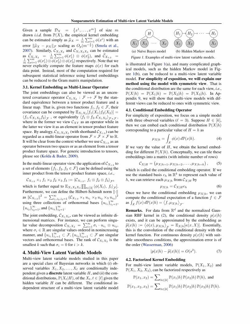
4. Multi-View Latent Variable ModelsMulti-view latent variable models studied in this paperare a special class of Bayesian networks in which (i) ob-served variables X1, X2, . . . , X` are conditionally inde-pendent given a discrete latent variableH , and (ii) the con-ditional distributions, P(Xt|H), of theXt, t ∈ [`] given thehidden variable H can be different. The conditional in-dependent structure of a multi-view latent variable model

H

X1 X2 · · · X`

(a) Naıve Bayes model

H1 H2 · · · H`

X1 X2 X`

(b) Hidden Markov model

Figure 1. Examples of multi-view latent variable models.

is illustrated in Figure 1(a), and many complicated graph-ical models, such as the hidden Markov model in Fig-ure 1(b), can be reduced to a multi-view latent variablemodel. For simplicity of exposition, we will explain ourmethod using the model with symmetric view. That isthe conditional distribution are the same for each view, i.e.,P(X|h) = P(X1|h) = P(X2|h) = P(X3|h). In Ap-pendix 9, we will show that multi-view models with dif-ferent views can be reduced to ones with symmetric view.

4.1. Conditional Embedding OperatorFor simplicity of exposition, we focus on a simple modelwith three observed variables (` = 3). Suppose H ∈ [k],then we can embed each conditional distribution P(X|h)corresponding to a particular value of H = h as

µX|h =

∫Xφ(x) dP(x|h). (4)

If we vary the value of H , we obtain the kernel embed-ding for different P(X|h). Conceptually, we can tile theseembeddings into a matrix (with infinite number of rows)

CX|H =(µX|h=1, µX|h=2, . . . , µX|h=k

), (5)

which is called the conditional embedding operator. If weuse the standard basis eh in Rk to represent each value ofh, we can retrieve each µX|h from CX|H by

µX|h = CX|Heh (6)

Once we have the conditional embedding µX|h, we cancompute the conditional expectation of a function f ∈ Fas∫X f(x) dP(x|h) =

⟨f, µX|h

⟩F .

Remarks. For data from Rd and the normalized Gaus-sian RBF kernel in (2), the conditional density p(x|h)exists, and it can be approximated by the embedding asp(x|h) :=

⟨φ(x), µX|h

⟩F = EX|h[κ(x,X)]. Essentially,

this is the convolution of the conditional density with thekernel function. For continuous density p(x|h) with suit-able smoothness conditions, the approximation error is ofthe order (Wasserman, 2006)

|p(x|h)− p(x|h)| = O(s2). (7)

4.2. Factorized Kernel EmbeddingFor multi-view latent variable models, P(X1, X2) andP(X1, X2, X3), can be factorized respectively as

P(x1, x2) =∑

h∈[k]P(x1|h)P(x2|h)P(h), and

P(x1, x2, x3) =∑

h∈[k]P(x1|h)P(x2|h)P(x3|h)P(h).


Since we assume the hidden variable H ∈ [k] is discrete,we let πh := P(h). Furthermore, if we apply Kroneckerdelta kernel δ(h, h′) with feature map eh, then the embed-dings for P(H)

CHH = EH [eH ⊗ eH ] =(πhδ(h, h

′))h,h′∈[k]

, and

CHHH = EH [eH ⊗ eH ⊗ eH ]

=(πh δ(h, h

′) δ(h′, h′′))h,h′,h′′∈[k]

are diagonal tensors. Making use of CHH and CHHH ,and the factorization of the distributions P(X1, X2) andP(X1, X2, X3), we obtain the factorization of the embed-ding of P(X1, X2) (second order embedding)

CX1X2=∑

h∈[k]

(µX1|h ⊗ µX2|h

)P(h)

=∑

h∈[k]

(CX|Heh

)⊗(CX|Heh

)P(h)

= CX|H(∑

h∈[k]eh ⊗ eh P(h)

)C>X|H

= CX|H CHH C>X|H , (8)

and that of P(X1, X2, X3) (third order embedding)

CX1X2X3 = CHHH ×1 CX|H ×2 CX|H ×3 CX|H . (9)

4.3. Identifiability of ParametersWe note that CX|H =

(µX|h=1, µX|h=2, . . . , µX|h=k

),

and the kernel embeddings for CX1X2and CX1X2X3

can bealternatively written as

CX1X2 =∑

h∈[k]πh · µX|h ⊗ µX|h, (10)

CX1X2X3 =∑

h∈[k]πh · µX|h ⊗ µX|h ⊗ µX|h. (11)

Allman et al. (2009) showed that, under mild conditions,a finite mixture of nonparametric product distributions isidentifiable. The multi-view latent variable model in (10)and (11) has the same form as a finite mixture of nonpara-metric product distribution, and therefore we can adapt All-man’s results to the current setting.Proposition 1 (Identifiability) Let P(X1, X2, X3) be amulti-view latent variable model, such that the condi-tional distributions P(X|h)h∈[k] are linearly indepen-dent. Then, the set of parameters

πh, µX|h

h∈[k]

areidentifiable from CX1X2X3

, up to label swapping of the hid-den variable H .Example 1. The probability vector of a discrete variableX ∈ [n], and the joint probability table of two discretevariables X1 ∈ [n] and X2 ∈ [n], are both kernel embed-dings. To see this, let the kernel be the Kronecker deltakernel κ(x, x′) = δ(x, x′) whose feature map φ(x) is thestandard basis of ex in Rn. The x-th dimension of ex is 1and 0 otherwise. Then

µX =(P(x = 1) . . . P(x = n)

)>,

CX1X2=(P(x1 = s, x2 = t)

)s,t∈[n]

.

We require that the conditional probability tableP (X|h)h∈[k] to have full column rank for identifi-ability in this case.

Example 2. Suppose we have a k-component mixtureof one dimensional spherical Gaussian distributions. TheGaussian components have identical covariance σ2, buttheir mean values are distinct. Note that this model isnot identifiable under the framework of Hsu & Kakade(2013) since the mean values are just scalars and therefore,rank deficient. However, if we embed the density func-tions using universal kernels such as Gaussian RBF kernel,it can be shown that the mixture model becomes identifi-able. This is because we are working with the entire densityfunction which are linearly independent from each other inthis case. Thus, the non-parametric framework allows us toincorporate a wider range of latent variable models.

Finally, we remark that the identifiability result in Propo-sition 1 can be extended to cases where the conditionaldistributions do not satisfy linear independence, i.e., theyare overcomplete, e.g. (Kruskal, 1977; De Lathauwer et al.,2007; Anandkumar et al., 2013b). However, in general, itis not tractable to learn such overcomplete models and wedo not consider them here.

5. Kernel AlgorithmWe first design a kernel algorithm to recover the param-eters,

πh, µX|h

h∈[k]

, of the multi-view latent variablemodel based on CX1X2 and CX1X2X3 . This can be eas-ily extended to the sample versions and this is discussedin Section 5.2. Again for simplicity of exposition, the al-gorithm is explained for symmetric view case. The moregeneral version is presented in Appendix 9.

5.1. Population CaseWe first derive the algorithm for the population case as ifwe could access the true operator CX1X2 and CX1X2X3 . Itsfinite sample counterpart will be presented in the next sec-tion. The algorithm can be thought of as a kernel general-ization of the algorithm in Anandkumar et al. (2013a) usingembedding representations.

Step 1. We perform eigen-decomposition of CX1X2,

CX1X2 =∑∞

i=1σi · ui ⊗ ui

where the eigen-values are ordered in non-decreasing man-ner. According to the factorization in Eq. (8), CX1X2

hasrank k. Let the leading eigenvectors corresponding to thelargest k eigen-value be Uk := (u1, u2, . . . , uk), and theeigen-value matrix be Sk := diag(σ1, σ2, . . . , σk). We de-fine the whitening operatorW := UkS−1/2

k which satisfies

W>CX1X2W = (W>CX|HC

1/2HH)(C1/2

HHC>X|HW) = I,

and M :=W>CX|HC1/2HH is an orthogonal matrix.


Step 2. We apply the whiten operator to the 3rd order ker-nel embedding CX1X2X3

T := CX1X2X3 ×1 (W>)×2 (W>)×3 (W>).

According to the factorization in Eq. (9), T = C−1/2HHH ×1

M ×2 M ×3 M, which is a tensor with orthogonal factors.Essentially, each column vi of M is an eigenvector of T .

Step 3. We use tensor power method to find the leadingk eigenvectors M for T (Anandkumar et al., 2012a). Thecorresponding k eigenvalues λ = (λ1, . . . , λk)> will thenbe equal to (P(h = 1)−1/2, . . . ,P(h = k)−1/2). The ten-sor power method is provided in the Appendix in Algo-rithm 2 for completeness.

Step 4. We recover the conditional embedding operator byundoing the whitening step

CX|H = (W>)†M diag(λ).

5.2. Finite Sample CaseGiven m observation DX1X2X3 = (xi1, xi2, xi3)i∈[m]

drawn i.i.d. from a multi-view latent variable modelP(X1, X2, X3), we now design a kernel algorithm to esti-mate the latent parameters from data. Although the empir-ical kernel embeddings can be infinite dimensional, we cancarry out the decomposition using just the kernel matrices.We denote the implicit feature matrix by

Φ := (φ(x11), . . . , φ(xm1 ), φ(x1

2), . . . , φ(xm2 )),

Ψ := (φ(x12), . . . , φ(xm2 ), φ(x1

1), . . . , φ(xm1 )),

and the corresponding kernel matrix by K = Φ>Φ andL = Ψ>Ψ respectively. And we denote K:x := Φ>φ(x)as a column vector containing the kernel between x anddata points in Φ. For three vectors ξ1, ξ2 and ξ3, denote thesymmetric tensor obtained from their outer product

⊗ [ξ1, ξ2, ξ3] := ξ1⊗ ξ2⊗ ξ3 + ξ3⊗ ξ1⊗ ξ2 + ξ2⊗ ξ3⊗ ξ1.Then the steps in the population case can be mapped one-by-one into kernel operations.

Step 1. We perform a kernel eigenvalue decomposition ofthe empirical 2nd order embedding

CX1X2:=

1

2m

∑m

i=1

(φ(xi1)⊗ φ(xi2) + φ(xi2)⊗ φ(xi1)

),

which can be expressed succinctly as CX1X2 = 12mΦΨ>.

Its leading k eigenvectors Uk = (u1, . . . , uk) lie in thespan of the column of Φ, i.e., Uk = Φ(β1, . . . , βk) withβ ∈ R2m. Then we can transform the eigen-value de-composition problem for an infinite dimensional matrix toa problem involving finite dimensional kernel matrices,

CX1X2C>X1X2

u = σ2 u ⇒ 1

4m2ΦΨ>ΨΦ>Φβ = σ2 Φβ

⇒ 1

4m2KLKβ = σ2Kβ.

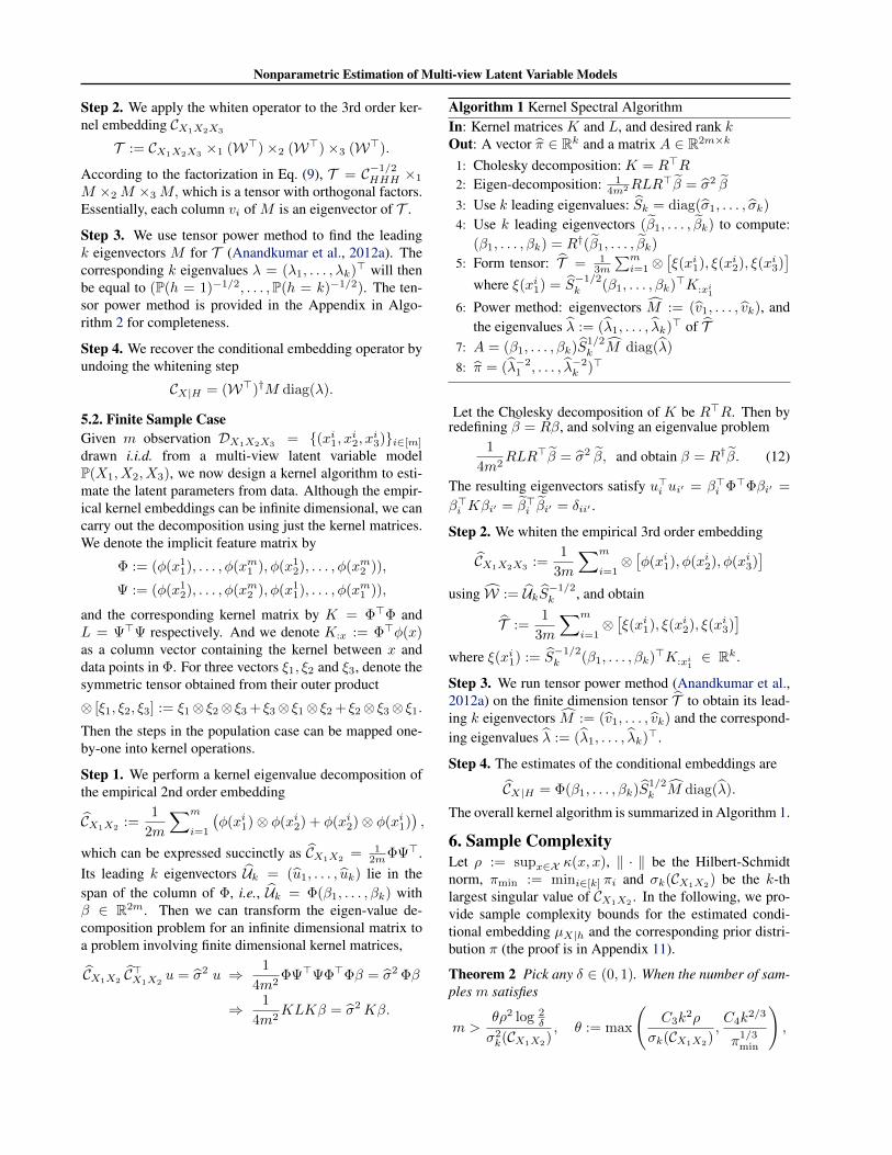
Algorithm 1 Kernel Spectral AlgorithmIn: Kernel matrices K and L, and desired rank kOut: A vector π ∈ Rk and a matrix A ∈ R2m×k

1: Cholesky decomposition: K = R>R

2: Eigen-decomposition: 14m2RLR

>β = σ2 β

3: Use k leading eigenvalues: Sk = diag(σ1, . . . , σk)

4: Use k leading eigenvectors (β1, . . . , βk) to compute:(β1, . . . , βk) = R†(β1, . . . , βk)

5: Form tensor: T = 13m

∑mi=1⊗

[ξ(xi1), ξ(xi2), ξ(xi3)

]where ξ(xi1) = S

−1/2k (β1, . . . , βk)>K:xi1

6: Power method: eigenvectors M := (v1, . . . , vk), andthe eigenvalues λ := (λ1, . . . , λk)> of T

7: A = (β1, . . . , βk)S1/2k M diag(λ)

8: π = (λ−21 , . . . , λ−2

k )>

Let the Cholesky decomposition of K be R>R. Then byredefining β = Rβ, and solving an eigenvalue problem

1

4m2RLR>β = σ2 β, and obtain β = R†β. (12)

The resulting eigenvectors satisfy u>i ui′ = β>i Φ>Φβi′ =

β>i Kβi′ = β>i βi′ = δii′ .

Step 2. We whiten the empirical 3rd order embedding

CX1X2X3:=

1

3m

∑m

i=1⊗[φ(xi1), φ(xi2), φ(xi3)

]using W := UkS−1/2

k , and obtain

T :=1

3m

∑m

i=1⊗[ξ(xi1), ξ(xi2), ξ(xi3)

]where ξ(xi1) := S

−1/2k (β1, . . . , βk)>K:xi1

∈ Rk.

Step 3. We run tensor power method (Anandkumar et al.,2012a) on the finite dimension tensor T to obtain its lead-ing k eigenvectors M := (v1, . . . , vk) and the correspond-ing eigenvalues λ := (λ1, . . . , λk)>.

Step 4. The estimates of the conditional embeddings are

CX|H = Φ(β1, . . . , βk)S1/2k M diag(λ).

The overall kernel algorithm is summarized in Algorithm 1.

6. Sample ComplexityLet ρ := supx∈X κ(x, x), ‖ · ‖ be the Hilbert-Schmidtnorm, πmin := mini∈[k] πi and σk(CX1X2

) be the k-thlargest singular value of CX1X2

. In the following, we pro-vide sample complexity bounds for the estimated condi-tional embedding µX|h and the corresponding prior distri-bution π (the proof is in Appendix 11).

Theorem 2 Pick any δ ∈ (0, 1). When the number of sam-ples m satisfies

m >θρ2 log 2

δ

σ2k(CX1X2

), θ := max

(C3k

2ρ

σk(CX1X2),C4k

2/3

π1/3min

),


for some constants C3, C4 > 0, and the number of itera-tions N and the number of random initialization vectors L(drawn uniformly on the sphere Sk−1) satisfy

N ≥ C2 ·(

log(k) + log log( 1√πminεT

)),

for constant C2 > 0 and L = poly(k) log(1/δ), the robustpower method in (Anandkumar et al., 2012a) yields eigen-pairs (λi, vi) such that there exists a permutation η, withprobability 1− 4δ, we have

‖π−1/2j µX|h=j − (β1, . . . , βk)S

1/2k vη(j)‖F ≤ 8εT · π−1/2

j ,

|π−1/2j − λη(j)| ≤ 5εT , ∀j ∈ [k],

and ‖T −∑kj=1 λj φ

⊗3j ‖ ≤ 55εT where εT := ‖T − T ‖

is the tensor perturbation bound

εT ≤8ρ1.5

√log 2

δ√mσ1.5

k (CX1X2)

+512√

2ρ3(log 2

δ

)1.5m1.5 σ3

k(CX1X2)√πmin

Proof Sketch: we note that our proof is different fromthose in Anandkumar et al. (2012a) which only analyzethe perturbation of the tensor decomposition. Our prooffurther takes into account the error introduced by theapproximate whitening step, and its effects to the tensordecomposition.

Remark 1: We note that the sample complexity ispoly(k, ρ, 1/πmin, 1/σk(CX1X2

)) of a low order, and inparticular, it is O(k2), when the other parameters are fixed.For the special case of discrete measurements, where thekernel κ(x, x′) = δ(x, x′), we have ρ = 1. Note that thesample complexity depends in this case only on the num-ber of components k and not on the dimensionality of theobserved state space. Thus, the robust tensor method hasefficient sample and computational complexities for non-parametric latent variable estimation.

Remark 2: Theorem 2 also gives us an error bound forestimating the integral of a function f ∈ F with respect toa mixture component in unsupervised fashion. That is∣∣∣∣∫

Xf(x) dP(x|h)−

⟨f, µX|h

⟩F

∣∣∣∣≤‖f‖F

∥∥µX|h − µX|h∥∥F = O(

1√m

)assuming ‖f‖F is bounded and ρ/σk = O(1).

Remark 3: For x ∈ Rd and the normalized Gaussian RBFkernel in (2), the recovered conditional embedding µX|hcan be used to estimate the conditional density, p(x|h) ≈p(x|h) :=

⟨φ(x), µX|h

⟩F . In this case, the error can be

decomposed into two terms

|p(x|h)− p(x|h)| ≤ |p(x|h)− p(x|h)|︸︷︷︸O(s2) bias as in (7)

+ |p(x|h)− p(x|h)|︸︷︷︸estimation error

where s is kernel bandwidth and p is the density convolvedwith the kernel function. The estimation error is boundedby |p(x|h) − p(x|h)| ≤ ‖φ(x)‖F‖µX|h − µX|h‖F =

O(ρ1/2 · m−1/2) = O(s−d/2m−1/2) assuming ρ/σk =O(1) and using ρ = s−d. Combining the two sources oferrors, we obtain a finite sample bound for conditional den-sity estimation. That is, with high probability,

|p(x|h)− p(x|h)| = O(s2 + s−d/2m−1/2)

Then we have |p(x|h) − p(x|h)| = O(m−2/(4+d)) if webalance the two terms by setting s = O(m−1/(4+d)).

7. DiscussionWe note that our algorithm and theoretical results can alsobe generalized to the settings of latent variable models withDirichlet priors and nonparametric independent componentanalysis (ICA) as in Anandkumar et al. (2012a). In the firstsetting, a Dirichlet prior is placed on the mixing weights πof the multi-view latent variables,

P(π) =Γ(θ0)∏i∈[k] Γ(θi)

∏i∈[k]

πθi−1i

where θ0 =∑i∈[k] θi with θi > 0, and Γ(·) is the Gamma

function. In this case, we only need to modify the sec-ond and third order kernel embedding CX1X2 and T respec-tively, and then Algorithm 1 applies. In the nonparametricICA setting, the feature map φ(X) of an observed variableX is assumed to be generated from a latent vector H ∈ Rkwith independent coordinates via an operatorA : Rk 7→ F ,

φ(X) := AH + Z

where Z is a zero mean random vector independent of H .In this case, we need to start with a modified 4-th orderkernel embedding, and then reduce to a multi-view problemand estimate A via Algorithm 1.

8. ExperimentsMethods. We compared our kernel spectral algorithm withfour alternatives

1. The EM algorithm for mixture of Gaussians. The EMalgorithm is not guaranteed to find the global solutionin each trial. Thus we randomly initialize it 10 times.

2. The EM-like algorithm for mixture of nonparametricdensities (Benaglia et al., 2009). We initialize the al-gorithm with k-means as Benaglia et al. (2009).

3. The spectral algorithm for mixture of spherical Gaus-sians (Hsu & Kakade, 2013). Their assumption is re-strictive: the centers of the Gaussian need to span a k-dimension subspace, thus it is not applicable for rankdeficiency case where k ≥ l.

4. A discretization based spectral algorithm (Kasahara& Shimotsu, 2010). This algorithm approximates thejoint distribution of the observed variables with his-togram and then applies the spectral algorithm to re-cover the discretized conditional density.


Both our method and the (Benaglia et al., 2009) have ahyper-parameter, kernel bandwidth, which we selected foreach view separately using cross-validation.

8.1. Synthetic DataWe generated three-dimensional synthetic data from vari-ous mixture models. The variables corresponding to thedimensions are independent given the latent component in-dicator. More specifically, we explored two settings (1)Gaussian conditional densities with different variances; (2)Mixture of Gaussian and shifted Gamma conditional den-sities. The shifted Gamma distribution has density

p(x|h) =(x− µ)(d−1)e−x/θ

θdΓ(d), x ≥ µ

where we chose the shape parameter d ≤ 1 such that den-sity is very skewed. Furthermore, we chose the mean andvariance parameters of the Gaussian/Gamma density suchthat component pair-wise overlap is relatively small ac-cording to the Fisher ratio (µ1−µ2)2

σ21+σ2

2.

We also varied the number of samples m for the observedvariables X1, X2 and X3 from 50 to 10, 000, and exper-imented with k = 2, 3, 4 or 8 mixture components. Themixture proportion for the h-th component is set to beπh = 2h

κ(k+1) , ∀h ∈ [k] (unbalanced). It is worth notingthat as k becomes larger, it is more difficult to recover pa-rameters. This is because only a small number of data willbe generated for the first several clusters. For every n, kin each setting, we randomly generated 10 sets of samplesand reported the average results. We note that the valuesfor the latent variables are not given to the algorithms,and hence this is an unsupervised setting to recover theconditional density p(x|h) and the ratio p(h).

Error measure. We measured the performance of al-gorithms by the following weighted `2 norm difference

MSE :=∑kh=1 πh

√∑m′

j=1(p(xj |h)− p(xj |h))2, where

xjj∈[m] is a set of uniformly-spaced test points.

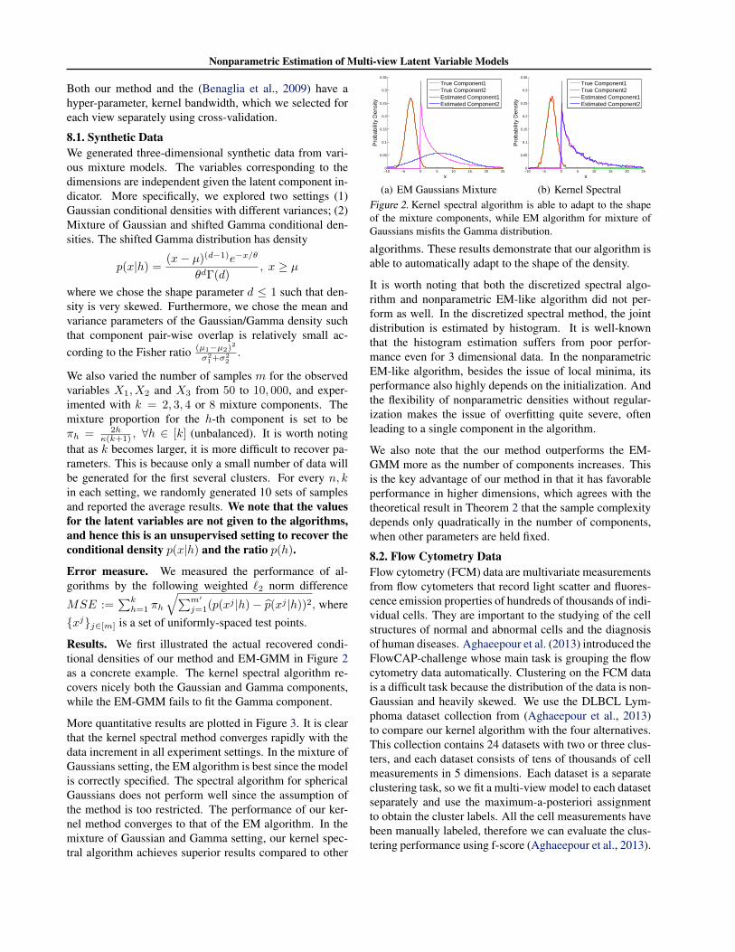
Results. We first illustrated the actual recovered condi-tional densities of our method and EM-GMM in Figure 2as a concrete example. The kernel spectral algorithm re-covers nicely both the Gaussian and Gamma components,while the EM-GMM fails to fit the Gamma component.

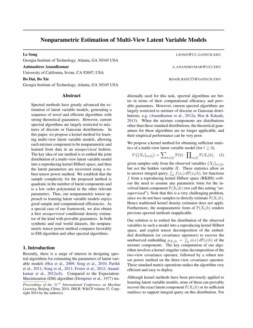
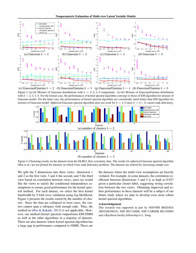
More quantitative results are plotted in Figure 3. It is clearthat the kernel spectral method converges rapidly with thedata increment in all experiment settings. In the mixture ofGaussians setting, the EM algorithm is best since the modelis correctly specified. The spectral algorithm for sphericalGaussians does not perform well since the assumption ofthe method is too restricted. The performance of our ker-nel method converges to that of the EM algorithm. In themixture of Gaussian and Gamma setting, our kernel spec-tral algorithm achieves superior results compared to other

−10 −5 0 5 10 15 20 250

0.05

0.1

0.15

0.2

0.25

0.3

0.35

x

Pro

babi

lity

Den

sity

True Component1True Component2Estimated Component1Estimated Component2

(a) EM Gaussians Mixture

−10 −5 0 5 10 15 20 250

0.05

0.1

0.15

0.2

0.25

0.3

0.35

x

Pro

babi

lity

Den

sity

True Component1True Component2Estimated Component1Estimated Component2

(b) Kernel SpectralFigure 2. Kernel spectral algorithm is able to adapt to the shapeof the mixture components, while EM algorithm for mixture ofGaussians misfits the Gamma distribution.

algorithms. These results demonstrate that our algorithm isable to automatically adapt to the shape of the density.

It is worth noting that both the discretized spectral algo-rithm and nonparametric EM-like algorithm did not per-form as well. In the discretized spectral method, the jointdistribution is estimated by histogram. It is well-knownthat the histogram estimation suffers from poor perfor-mance even for 3 dimensional data. In the nonparametricEM-like algorithm, besides the issue of local minima, itsperformance also highly depends on the initialization. Andthe flexibility of nonparametric densities without regular-ization makes the issue of overfitting quite severe, oftenleading to a single component in the algorithm.

We also note that the our method outperforms the EM-GMM more as the number of components increases. Thisis the key advantage of our method in that it has favorableperformance in higher dimensions, which agrees with thetheoretical result in Theorem 2 that the sample complexitydepends only quadratically in the number of components,when other parameters are held fixed.

8.2. Flow Cytometry DataFlow cytometry (FCM) data are multivariate measurementsfrom flow cytometers that record light scatter and fluores-cence emission properties of hundreds of thousands of indi-vidual cells. They are important to the studying of the cellstructures of normal and abnormal cells and the diagnosisof human diseases. Aghaeepour et al. (2013) introduced theFlowCAP-challenge whose main task is grouping the flowcytometry data automatically. Clustering on the FCM datais a difficult task because the distribution of the data is non-Gaussian and heavily skewed. We use the DLBCL Lym-phoma dataset collection from (Aghaeepour et al., 2013)to compare our kernel algorithm with the four alternatives.This collection contains 24 datasets with two or three clus-ters, and each dataset consists of tens of thousands of cellmeasurements in 5 dimensions. Each dataset is a separateclustering task, so we fit a multi-view model to each datasetseparately and use the maximum-a-posteriori assignmentto obtain the cluster labels. All the cell measurements havebeen manually labeled, therefore we can evaluate the clus-tering performance using f-score (Aghaeepour et al., 2013).


0.05 0.1 0.2 0.5 1 2 5 100

1

2

3

4

5

6

7

8

9

sample size (× 103)

MS

E

EM GMMNonparametric EMKernel SpectralHistogram SpectralHsu et. al.

0.05 0.1 0.2 0.5 1 2 5 100

1

2

3

4

5

6


MS

E

0.05 0.1 0.2 0.5 1 2 5 100

0.5

1

1.5

2

2.5

3

3.5

4

4.5


MS

E

0.05 0.1 0.2 0.5 1 2 5 100

0.5

1

1.5

2

2.5

3


MS

E

(a) Gaussian k = 2 (b) Gaussian k = 3 (c) Gaussian k = 4 (d) Gaussian k = 8

0.05 0.1 0.2 0.5 1 2 5 100

1

2

3

4

5

6

7

8

9


MS

E

0.05 0.1 0.2 0.5 1 2 5 100

1

2

3

4

5

6

7


MS

E

0.05 0.1 0.2 0.5 1 2 5 100.5

1

1.5

2

2.5

3

3.5

4

4.5

5


MS

E

0.05 0.1 0.2 0.5 1 2 5 100

1

2

3

4

5

6


MS

E

(e) Gaussian/Gamma k = 2 (f) Gaussian/Gamma k = 3 (g) Gaussian/Gamma k = 4 (h) Gaussian/Gamma k = 8Figure 3. (a)-(d) Mixture of Gaussian distributions with k = 2, 3, 4, 8 components. (e)-(h) Mixture of Gaussian/Gamma distributionwith k = 2, 3, 4, 8. For the former case, the performances of kernel spectral algorithm converge to those of EM algorithm for mixture ofGaussian model. For the latter case, the performances of kernel spectral algorithm are consistently much better than EM algorithm formixture of Gaussian model. Spherical Gaussian spectral algorithm does not work for k = 4, 8 since k > l(= 3) causes rank deficiency.

1 2 3 4 5 6 7 80.4

0.6

0.8

1.0

Datasets

f−sc

ore

EM GMMNonparametric EMKernel SpectralHistogram SpectralHsu et al.

(a) number of clusters k = 2

2 4 6 8 10 12 14 160.4

0.6

0.8

1.0

Datasets

f−sc

ore

(b) number of clusters k = 3

Figure 4. Clustering results on the datasets from the DLBCL flow cytometry data. The results for spherical Gaussian spectral algorithm(Hsu et al.) are not plotted for datasets on which it has rank deficiency problem. The datasets are ordered by increasing sample size.

We split the 5 dimensions into three views: dimension 1and 2 as the first view, 3 and 4 the second, and 5 the thirdview based on correlation between views, since we wouldlike the views to satisfy the conditional independence as-sumptions to ensure good performance for the kernel spec-tral method. For each dataset, we select the best kernelbandwidth by 5-fold cross validation using log-likelihood.Figure 4 presents the results sorted by the number of clus-ters. Since the data are collapsed in most cases, the cen-ters cannot span a subspace with enough rank. Thus, themethod in (Hsu & Kakade, 2013) is not applicable. How-ever, our method (kernel spectral) outperforms EM-GMMas well as the other algorithms in a majority of datasets.There are also datasets where kernel spectral algorithm hasa large gap in performance compared to GMM. These are

the datasets where the multi-view assumptions are heavilyviolated. For example, in some datasets, the correlation co-efficient between dimensions 3 and 5 is as high as 0.927given a particular cluster label, suggesting strong correla-tion between the two views. Obtaining improved and ro-bust performance in these datasets will be a subject of ourfuture study where we plan to develop even more robustkernel spectral algorithms.

AcknowledgementThis research was supported in part by NSF/NIH BIGDATA1R01GM108341, NSF IIS1116886, NSF CAREER IIS1350983and a Raytheon faculty fellowship to L. Song.


ReferencesAghaeepour, Nima, Finak, Greg, Consortium, The Flow-

CAP, Consortium, The DREAM, Hoos, Holger, Mos-mann, Tim R, Brinkman, Ryan, Gottardo, Raphael, andScheuermann, Richard H. Critical assessment of auto-mated flow cytometry data analysis techniques. NatureMethods, 10(3):228–238, 2013.

Allman, Elizabeth, Matias, Catherine, and Rhodes, John.Identifiability of parameters in latent structure modelswith many observed variables. The Annals of Statistics,37(6A):3099–3132, 2009.

Anandkumar, A., Ge, R., Hsu, D., Kakade, S. M., and Tel-garsky, M. Tensor Methods for Learning Latent VariableModels. Available at arXiv:1210.7559, Oct. 2012a.

Anandkumar, A., Ge, R., Hsu, D., and Kakade, S. M. ATensor Spectral Approach to Learning Mixed Member-ship Community Models. ArXiv 1302.2684, Feb. 2013a.

Anandkumar, A., Hsu, D., Janzamin, M., and Kakade,S. M. When are Overcomplete Topic Models Identi-fiable? Uniqueness of Tensor Tucker Decompositionswith Structured Sparsity. ArXiv 1308.2853, Aug. 2013b.

Anandkumar, Animashree, Foster, Dean P., Hsu, Daniel,Kakade, Sham M., and Liu, Yi-Kai. A spectral al-gorithm for latent dirichlet allocation. Available atarXiv:1204.6703, 2012b.

Benaglia, Tatiana, Chauveau, Didier, and Hunter, David R.An em-like algorithm for semi-and nonparametric esti-mation in multivariate mixtures. Journal of Computa-tional and Graphical Statistics, 18(2):505–526, 2009.

De Lathauwer, L., Castaing, J., and Cardoso, J.-F. Fourth-order cumulant-based blind identification of underdeter-mined mixtures. IEEE Tran. on Signal Processing, 55:2965–2973, June 2007.

Dempster, A. P., Laird, N. M., and Rubin, D. B. Maximumlikelihood from incomplete data via the EM algorithm.Journal of the Royal Statistical Society B, 39(1):1–22,1977.

Foster, D.P., Rodu, J., and Ungar, L.H. Spectral di-mensionality reduction for hmms. Arxiv preprintarXiv:1203.6130, 2012.

Hsu, D., Kakade, S., and Zhang, T. A spectral algorithm forlearning hidden markov models. In Proc. Annual Conf.Computational Learning Theory, 2009.

Hsu, Daniel and Kakade, Sham M. Learning mixtures ofspherical gaussians: moment methods and spectral de-compositions. In Proceedings of the 4th conference onInnovations in Theoretical Computer Science, ITCS ’13,pp. 11–20.

Kasahara, Hiroyuki and Shimotsu, Katsumi. Nonparamet-ric identification of multivariate mixtures. Journal of theRoyal Statistical Society - Series B, 2010.

Kolda, Tamara G. and Bader, Brett W. Tensor decompo-sitions and applications. SIAM Review, 51(3):455–500,2009.

Kruskal, J.B. Three-way arrays: Rank and uniqueness oftrilinear decompositions, with application to arithmeticcomplexity and statistics. Linear algebra and its appli-cations, 18(2):95–138, 1977.

Parikh, A., Song, L., and Xing, E. P. A spectral algorithmfor latent tree graphical models. In Proceedings of theInternational Conference on Machine Learning, 2011.

Rosasco, L., Belkin, M., and Vito, E.D. On learning withintegral operators. Journal of Machine Learning Re-search, 11:905–934, 2010.

Scholkopf, B., Tsuda, K., and Vert, J.-P. Kernel Methodsin Computational Biology. MIT Press, Cambridge, MA,2004.

Sgouritsa, Eleni, Janzing, Dominik, Peters, Jonas, andScholkopf, Bernhard. Identifying finite mixtures of non-parametric product distributions and causal inference ofconfounders. In Conference on Uncertainty on ArtificialIntelligence (UAI), 2013.

Smola, A. J., Gretton, A., Song, L., and Scholkopf, B.A Hilbert space embedding for distributions. In Pro-ceedings of the International Conference on Algorith-mic Learning Theory, volume 4754, pp. 13–31. Springer,2007.

Song, L. and Dai, B. Robust low rank kernel embeddingof multivariate distributions. In Neural Information Pro-cessing Systems (NIPS), 2013.

Song, L., Boots, B., Siddiqi, S., Gordon, G., and Smola,A. J. Hilbert space embeddings of hidden markov mod-els. In International Conference on Machine Learning,2010.

Song, L., Parikh, A., and Xing, E.P. Kernel embeddingsof latent tree graphical models. In Advances in NeuralInformation Processing Systems, volume 25, 2011.

Sriperumbudur, B., Gretton, A., Fukumizu, K., Lanckriet,G., and Scholkopf, B. Injective Hilbert space embed-dings of probability measures. In Proc. Annual Conf.Computational Learning Theory, pp. 111–122, 2008.

Wasserman, L. All of Nonparametric Statistics. Springer,2006.


Appendix

9. SymmetrizationWe presented the kernel algorithm for learning the multi-view latent variable model where the views have identical con-ditional distributions. In this section, we will extend it to the general case where the views are different. Without loss ofgenerality, we will consider recover the operator µX3|h for conditional distribution P(X3|h). The same strategy applies toother views. The idea is to reduce the multi-view case to the identical-view case based on a method by (Anandkumar et al.,2012b).

Given the observations DX1X2X3 = (xi1, xi2, xi3)i∈[m] drawn i.i.d. from a multi-view latent variable modelP(X1, X2, X3), let the kernel matrix associated with X1, X2 and X3 be K, L and G respectively and the correspondingfeature map be φ, ψ and υ respectively. Furthermore, let the corresponding feature matrix be Φ = (φ(x1

1), . . . , φ(xm1 )),Ψ = (φ(x1

2), . . . , φ(xm2 )) and Υ = (φ(x13), . . . , φ(xm3 )). Then, we have the empirical estimation of the second/third-order

embedding as

CX1X2=

1

mΦΨ>, CX3X1

=1

mΥΦ>, CX2X3

=1

mΨΥ>

CX1X2X3:=

1

mIn ×1 Φ×2 Ψ×3 Υ

Find two arbitrary matrices A,B ∈ Rk×∞, so that ACX1X2B> is invertible. Theoretically, we could randomly select k

columns from Φ and Ψ and set A = Φ>k ,B = Ψ>k . In practial, the first k leading eigenvector directions of respect RKHSworks better. Then, we have

CX1X2=

1

mΦ>k ΦΨ>Ψk =

1

mK>nkLnk

CX3X1= CX3X1

Φk =1

mΥKnk

CX3X2= CX3X2

Ψk =1

mΥLnk

CX1X2X3 = CX1X2X3 ×1 Φ>k ×2 Ψ>k =1

mIn ×1 K

>nk ×2 L

>nk ×3 Υ

Based on these matrices, we could reduce to a single view

Pair3 = CX3X1(C>X1X2

)−1CX3X2

=1

mΥKnk(L>nkKnk)−1L>nkΥ> =

1

mΥHΥ>

where H = Knk(L>nkKnk)−1L>nk.

Assume the leading k eigenvectors νk lie in the span of the column of Υ, i.e., νk = Υβk where βk ∈ Rm×1

Pair3ν = λν ⇒ (Pair3)>Pair3ν = λ2ν

⇒ 1

m2ΥH>Υ>ΥHΥ>ν = λ2ν

⇒ 1

m2ΥH>GHGβ = λ2Υβ

⇒ 1

m2GH>GHGβ = λ2Gβ

Then, we symmetrize and whiten the third-order embedding

Triple3 =1

mCX1X2X3

×1 [CX3X2C−1X1X2

]×2 [CX3X1C−1X2X1

] (13)

Plug CX3X2 C−1X1X2

= ΥLnk(K>nkLnk)−1 and CX3X1 C−1X2X1

= ΥKnk(L>nkKnk)−1, we have


Triple3 =1

mIn ×1 ΥLnk(K>nkLnk)−1K>nk

×2ΥKnk(L>nkKnk)−1L>nk ×3 Υ

We multiply each mode with ΥβS− 1

2

k to whitening the data and apply power method to decompose it

T = Triple3 ×1 S− 1

2

k β>Υ> ×2 S− 1

2

k β>Υ> ×3 S− 1

2

k β>Υ>

=1

mIn ×1 S

− 12

k β>GLnk(K>nkLnk)−1K>nk ×2

S− 1

2

k β>GKnk(L>nkKnk)−1L>nk ×3 S− 1

2

k β>G

10. Robust Tensor Power MethodWe recap the robust tensor power method for finding the tensor eigen-pairs in Algorithm 2, analyzed in detail in (Anand-kumar et al., 2013a) and (Anandkumar et al., 2012a). The method computes the eigenvectors of a tensor through deflation,using a set of initialization vectors. Here, we employ random initialization vectors. This can be replaced with better ini-tialization vectors, in certain settings, e.g. in the community model, the neighborhood vectors provide better initializationand lead to stronger guarantees (Anandkumar et al., 2013a). Given the initialization vector, the method then runs a tensorpower update, and runs for N iterations to obtain an eigenvector. The successive eigenvectors are obtained via deflation.

Algorithm 2 λ,M ←TensorEigen(T , vii∈[k], N)

Input: Tensor T ∈ Rk×k×k, set of k initialization vectors vii∈[k], number of iterations N .Output: the estimated eigenvalue/eigenvector pairs λ,M, where λ = (λ1, . . . , λk)> is the vector of eigenvalues andM = (v1, . . . , vk) is the matrix of eigenvectors.for i = 1 to k do

for τ = 1 to k doθ0 ← vτ .for t = 1 to N doT ← T .for j = 1 to i− 1 (when i > 1) do

if |λj⟨θ

(τ)t , vj

⟩| > ξ then

T ← T − λjφ⊗3j .

end ifend forCompute power iteration update θ(τ)

t :=T (I,θ

(τ)t−1,θ

(τ)t−1)

‖T (I,θ(τ)t−1,θ

(τ)t−1)‖

end forend forLet τ∗ := arg maxτ∈LT (θ

(τ)N , θ

(τ)N , θ

(τ)N ).

Do N power iteration updates starting from θ(τ∗)N to obtain eigenvector estimate vi, and set λi := T (vi, vi, vi).

end forreturn the estimated eigenvalue/eigenvectors (λ,M).

11. Proof of Theorem 211.1. Recap of Perturbation Bounds for the Tensor Power Method

We now recap the result of Anandkumar et al. (2013a, Thm. 13) that establishes bounds on the eigen-estimates under goodinitialization vectors for the above procedure. Let T =

∑i∈[k] λivi, where vi are orthonormal vectors and λ1 ≥ λ2 ≥

. . . λk. Let T = T + E be the perturbed tensor with ‖E‖ ≤ εT . Recall that N denotes the number of iterations of thetensor power method. We call an initialization vector u to be (γ,R0)-good if there exists vi such that 〈u, vi〉 > R0 and


| 〈u, vi〉 | −maxj<i | 〈u, vj〉 | > γ| 〈u, vi〉 |. Choose γ = 1/100.

Theorem 3 There exists universal constants C1, C2 > 0 such that the following holds.

εT ≤ C1 · λminR20, N ≥ C2 ·

(log(k) + log log

(λmax

εT

)), (14)

Assume there is at least one good initialization vector corresponding to each vi, i ∈ [k]. The parameter ξ for choosingdeflation vectors in each iteration of the tensor power method in Procedure 2 is chosen as ξ ≥ 25εT . We obtain eigenvalue-eigenvector pairs (λ1, v1), (λ2, v2), . . . , (λk, vk) such that there exists a permutation η on [k] with

‖vη(j) − vj‖ ≤ 8εT /λη(j), |λη(j) − λj | ≤ 5εT , ∀j ∈ [k],

and ∥∥∥∥∥∥T −k∑j=1

λj v⊗3j

∥∥∥∥∥∥ ≤ 55εT .

In the sequel, we establish concentration bounds that allows us to translate the above condition on tensor perturbation (14)to sample complexity bounds.

11.2. Concentration Bounds

11.2.1. ANALYSIS OF WHITENING

Recall that we use the covariance operator CX1X2for whitening the 3rd order embedding CX1,X2,X3

. We first analyze theperturbation in whitening when sample estimates are employed.

Let CX1X2denote the sample covariance operator between variables X1 and X2, and let

B := 0.5(CX1X2 + C>X1X2) = U SU>

denote the SVD. Let Uk and Sk denote the restriction to top-k eigen-pairs, and let Bk := UkSkU>k . Recall that thewhitening matrix is given by W := UkS−1/2

k . Now W whitens Bk, i.e. W>BkW = I .

Now consider the SVD ofW>CX1X2

W = ADA>,

and defineW := WAD−1/2A>,

andW whitens CX1X2 sinceW>CX1X2W = I . Recall that by exchangeability assumption,

CX1,X2=

k∑j=1

πj · µX|j ⊗ µX|j = M Diag(π)M>, (15)

where the j th column of M , Mj = µX|j .

We now establish the following perturbation bound on the whitening procedure. Recall from (25), εpairs :=∥∥∥CX1,X2 − CX1,X2

∥∥∥. Let σ1(·) ≥ σ2(·) . . . denote the singular values of an operator.

Lemma 4 (Whitening perturbation) Assuming that εpairs < 0.5σk(CX1X2),

εW := ‖Diag(π)1/2M>(W −W)‖ ≤ 4εpairsσk(CX1X2

)(16)

Remark: Note that σk(CX1X2) = σ2

k(M).

Proof: The proof is along the lines of Lemma 16 of (Anandkumar et al., 2013a), but adapted to whitening using thecovariance operator here.

‖Diag(π)1/2M>(W −W)‖ = ‖Diag(π)1/2M>W (AD1/2A> − I)‖≤ ‖Diag(π)1/2M>W‖‖D1/2 − I‖.


SinceW whitens CX1X2= M Diag(π)M>, we have that ‖Diag(π)1/2M>W‖ = 1. Now we control ‖D1/2 − I‖. Let

E := CX1,X2− Bk, where recall that B = 0.5(CX1,X2

+ C>X1X2) and Bk is its restriction to top-k singular values. Thus,

we have ‖E‖ ≤ εpairs + σk+1(B) ≤ 2εpairs. We now have

‖D1/2 − I‖ ≤ ‖(D1/2 − I)(D1/2 + I)‖ ≤ ‖D − I‖

= ‖ADA> − I‖ = ‖W>CX1X2W − I‖

= ‖W>EW‖ ≤ ‖W‖2(2εpairs).

Now

‖W2‖ ≤ 1

σk(CX1X2)≤ 2

σk(CX1X2),

when εpairs < 0.5σk(CX1X2). 2

11.2.2. TENSOR CONCENTRATION BOUNDS

Recall that the whitened tensor from samples is given by

T := CX1X2X3×1 (W>)×2 (W>)×3 (W>).

We want to establish its perturbation from the whitened tensor using exact statistics

T := CX1X2X3 ×1 (W>)×2 (W>)×3 (W>).

Further, we haveCX1X2X3

=∑h∈[k]

πh · µX|h ⊗ µX|h ⊗ µX|h (17)

Let εtriples := ‖CX1X2X3− CX1X2X3

‖. Let πmin := minh∈[k] πh.

Lemma 5 (Tensor perturbation bound) Assuming that εpairs < 0.5σk(CX1X2), we have

εT := ‖T − T ‖ ≤ 2√

2εtriplesσk(CX1X2)1.5

+ε3W√πmin

. (18)

Proof: Define intermediate tensor

T := CX1X2X3×1 (W>)×2 (W>)×3 (W>).

We will bound ‖T − T ‖ and ‖T − T ‖ separately.

‖T − T ‖ ≤ ‖CX1,X2,X2− CX1,X2,X3

‖‖W‖3 ≤ 2√

2εtriplesσk(CX1X2)1.5

,

using the bound on ‖W‖ in Lemma 4. For the other term, first note that

CX1,X2,X3=∑h∈[k]

πh ·Mh ⊗Mh ⊗Mh,

‖T − T ‖ = ‖CX1X2X3 ×1 (W −W)> ×2 (W −W)> ×3 (W −W)>‖

≤ ‖Diag(π)1/2M>(W −W)‖3√πmin

=ε3W√πmin

2

Proof of Theorem 2: We obtain a condition on the above perturbation εT in (18) by applying Theorem 3 as εT ≤C1λminR

20. Here, we have λi = 1/

√πi ≥ 1. For random initialization, we have that R0 ∼ 1/

√k, with probability 1 − δ

using poly(k) poly(1/δ) trials, see Thm. 5.1 in (Anandkumar et al., 2012a). Thus, we require that εT ≤ C1

k . Summarizing,


we require for the following conditions to hold

εpairs ≤ 0.5σk(CX1X2), εT ≤

C1

k. (19)

We now substitute for εpairs and εtriples in (18) using Lemma 6 and Lemma 7.

From Lemma 6, we have that

εpairs 62√

2ρ√

log 2δ√

m,

with probability 1− δ. It is required that εpairs < 0.5σk(CX1,X2), which yields that

m >32ρ2 log 2

δ

σ2k(CX1,X2

). (20)

Further we require that εT ≤ C1/k, which implies that each of the terms in (18) is less than C/k, for some constant C.Thus, we have

2√

2εtriplesσ1.5k (CX1,X2

)<C

k⇒ m >

C3k2ρ3 log 2

δ

σ3k(CX1,X2

),

for some constant C3 with probability 1− δ from Lemma 7. Similarly for the second term in (18), we have

ε3W√πmin

<C

k,

and from Lemma 4, this implies that

εpairs ≤C ′π

1/6minσk(CX1,X2

)

k1/3,

Thus, we have

m >C4k

23 ρ2 log 2

δ

π13

minσ2k(CX1,X2)

,

for some other constant C4 with probability 1− δ. Thus, we have the result in Theorem 2.

2

11.2.3. CONCENTRATION BOUNDS FOR EMPIRICAL OPERATORS

Concentration results for the singular value decomposition of empirical operators.

Lemma 6 (Concentration bounds for pairs) Let ρ := supx∈Ω k(x, x), and ‖ · ‖ be the Hilbert-Schmidt norm, we havefor

εpairs :=∥∥∥CX1X2

− CX1X2

∥∥∥ , (21)

Pr

εpairs 6 2√

2ρ√

log 2δ√

m

> 1− δ. (22)

Proof We will use similar arguments as in (Rosasco et al., 2010) which deals with symmetric operator. Let ξi be definedas

ξi = φ(xi1)⊗ φ(xi2)− CX1,X2. (23)

It is easy to see that E[ξi] = 0. Further, we have

supx1,x2

‖φ(x1)⊗ φ(x2)‖2 = supx1,x2

k(x1, x1)k(x2, x2) 6 ρ2, (24)

which implies that ‖CX1X2‖ 6 ρ, and ‖ξi‖ 6 2ρ. The result then follows from the Hoeffding’s inequality in Hilbert space.

Similarly, we have the concentration bound for 3rd order embedding.


Lemma 7 (Concentration bounds for triples) Let ρ := supx∈Ω k(x, x), and ‖ · ‖ be the Hilbert-Schmidt norm, we havefor

εtriples :=∥∥∥CX1X2X3

− CX1X2X3

∥∥∥ , (25)

Pr

εtriples 6 2√

2ρ3/2√

log 2δ√

m

> 1− δ. (26)

Proof We will use similar arguments as in (Rosasco et al., 2010) which deals with symmetric operator. Let ξi be definedas

ξi = φ(xi1)⊗ φ(xi2)⊗ φ(xi3)− CX1X2X3. (27)

It is easy to see that E[ξi] = 0. Further, we have

supx1,x2,x3

‖φ(x1)⊗ φ(x2)⊗ φ(x3)‖2 = supx1,x2,x3

k(x1, x1)k(x2, x2)k(x3, x3) 6 ρ3, (28)

which implies that ‖CX1X2X3‖ 6 ρ3/2, and ‖ξi‖ 6 2ρ3/2. The result then follows from the Hoeffding’s inequality inHilbert space.

12. Experiment on Single Conditional DistributionWe also did some experiments for three-dimensional synthetic data that each view has the same conditional distribution.We generated the data from two settings:

1. Mixture of Gaussian conditional density;

2. Mixture of Gaussian and shifted Gamma conditional density.

The mixture proportion and other experiment settings are exact same as the experiment in the main text. The only differenceis that the conditional densities for each view here are the identical. We use the same measure to evaluate the performance.The empirical results are plotted in Figure 5.

As we expected, the behavior of the proposed method is similar to the results in different conditional densities case. Inmixture of Gaussians, our algorithm converges to the EM GMM resuls. And in the mixture of Gaussian/shift Gamma, ouralgorithm consistently better to other alternatives in most cases, except k = 3 where our method achieve comparable tononparametric EM algorithm.


0.05 0.1 0.2 0.5 1 2 5 100

1

2

3

4

5

6

7

8


MS

E

EM GMMNonparametric EMKernel SpectralHistgram SpectralHsu et. al.

0.05 0.1 0.2 0.5 1 2 5 100

1

2

3

4

5

6

7


MS

E

0.05 0.1 0.2 0.5 1 2 5 100

1

2

3

4

5

6


MS

E

0.05 0.1 0.2 0.5 1 2 5 100

0.5

1

1.5

2

2.5

3


MS

E

(a) Gaussian k = 2 (b) Gaussian k = 3 (c) Gaussian k = 4 (d) Gaussian k = 8

0.05 0.1 0.2 0.5 1 2 5 100

1

2

3

4

5

6

7

8


MS

E

EM GMM

Nonparametric EMKernel SpectralHistgram SpectralHsu et. al.

0.05 0.1 0.2 0.5 1 2 5 100

1

2

3

4

5

6


MS

E

0.05 0.1 0.2 0.5 1 2 5 100.5

1

1.5

2

2.5

3

3.5

4

4.5


MS

E

0.05 0.1 0.2 0.5 1 2 5 100.5

1

1.5

2

2.5

3

3.5


MS

E

(e) Gaussian/Gamma k = 2 (f) Gaussian/Gamma k = 3 (g) Gaussian/Gamma k = 4 (h) Gaussian/Gamma k = 8

Figure 5. (a)-(d) Mixture of Gaussian distributions with k = 2, 3, 4, 8 components. (e)-(h) Mixture of Gaussian/Gamma distributionwith k = 2, 3, 4, 8. For the former case, the performance of kernel spectral algorithm converge to those of EM algorithm for mixtureof Gaussian model. For both cases, the performance of kernel spectral algorithm are consistently the best or comparable. SphericalGaussian spectral algorithm does not work for k = 4, 8, and hence not plotted.

Documents

Nonparametric Estimation of Multi-View Latent Variable Models