Embed Size (px)
Citation preview

Nonparametric Location Tests: One-Sample
Nathaniel E. Helwig
Assistant Professor of Psychology and StatisticsUniversity of Minnesota (Twin Cities)
Updated 04-Jan-2017
Nathaniel E. Helwig (U of Minnesota) Nonparametric Location Tests: One-Sample Updated 04-Jan-2017 : Slide 1

Copyright
Copyright c© 2017 by Nathaniel E. Helwig
Nathaniel E. Helwig (U of Minnesota) Nonparametric Location Tests: One-Sample Updated 04-Jan-2017 : Slide 2

Outline of Notes
1) Background Information:Hypothesis testingLocation testsOrder and rank statisticsOne-sample problem
2) Signed Rank Test (Wilcoxon):OverviewHypothesis testingEstimating locationConfidence intervals
3) Sign Test (Fisher):OverviewHypothesis testingEstimating locationConfidence intervals
4) Some Considerations:Choosing a location testUnivariate symmetryBivariate symmetry
Nathaniel E. Helwig (U of Minnesota) Nonparametric Location Tests: One-Sample Updated 04-Jan-2017 : Slide 3

Background Information
Background Information
Nathaniel E. Helwig (U of Minnesota) Nonparametric Location Tests: One-Sample Updated 04-Jan-2017 : Slide 4

Background Information Hypothesis Testing
Neyman-Pearson Hypothesis Testing Procedure
Hypothesis testing procedure (by Jerzy Neyman & Egon Pearson1):(a) Start with a null and alternative hypothesis (H0 and H1) about θ(b) Calculate some test statistic T from the observed data(c) Calculate p-value; i.e., probability of observing a test statistic as or
more extreme than T under the assumption H0 is true(d) Reject H0 if the p-value is below some user-determined threshold
Typically we assume observed data are from some known probabilitydistribution (e.g., Normal, t , Poisson, binomial, etc.).
1Egon Pearson was the son of Karl Pearson (very influential statistician).Nathaniel E. Helwig (U of Minnesota) Nonparametric Location Tests: One-Sample Updated 04-Jan-2017 : Slide 5

Background Information Hypothesis Testing
Confidence Intervals
In addition to testing H0, we may want to know how confident we canbe in our estimate of the unknown population parameter θ.
A symmetric 100(1− α)% confidence interval (CI) has the form:
θ ± T ∗1−α/2σθ
where θ is our estimate of θ, σθ is the standard error of θ, and T ∗1−α/2 isthe critical value of the test statistic, i.e., P(T ≤ T ∗1−α/2) = 1− α/2.
Interpreting Confidence Intervals:Correct: through repeated samples, e.g., 99 out of 100 confidenceintervals would be expected to contain true θ with α = .01Wrong: through one sample; e.g., there is a 99% chance theconfidence interval around my θ contains the true θ (with α = .01)
Nathaniel E. Helwig (U of Minnesota) Nonparametric Location Tests: One-Sample Updated 04-Jan-2017 : Slide 6
Background Information Location Tests
Definition of “Location Test”
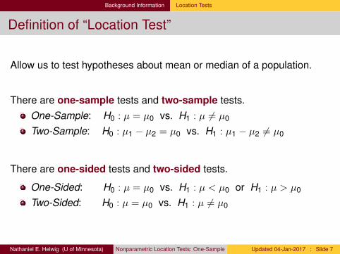
Allow us to test hypotheses about mean or median of a population.
There are one-sample tests and two-sample tests.One-Sample: H0 : µ = µ0 vs. H1 : µ 6= µ0
Two-Sample: H0 : µ1 − µ2 = µ0 vs. H1 : µ1 − µ2 6= µ0
There are one-sided tests and two-sided tests.
One-Sided: H0 : µ = µ0 vs. H1 : µ < µ0 or H1 : µ > µ0
Two-Sided: H0 : µ = µ0 vs. H1 : µ 6= µ0
Nathaniel E. Helwig (U of Minnesota) Nonparametric Location Tests: One-Sample Updated 04-Jan-2017 : Slide 7

Background Information Location Tests
Problems with Parametric Location Tests
Typical parametric location tests (e.g., Student’s t tests) focus onanalyzing mean differences.
Robustness: sample mean is not robust to outliersConsider a sample of data x1, . . . , xn with expectation µ <∞Suppose we fix x1, x2, . . . , xn−1 and let xn →∞Note x = 1
n∑n
i=1 xi →∞, i.e., one large outlier ruins sample mean
Generalizability: parametric tests are meant for particular distributionsAssume data are from some known distributionParametric inferences are invalid if assumption is wrong
Nathaniel E. Helwig (U of Minnesota) Nonparametric Location Tests: One-Sample Updated 04-Jan-2017 : Slide 8

Background Information Order and Rank Statistics
Order Statistics
Given a sample of data
X1, X2, X3, . . . ,Xn
from some cdf F , the order statistics are typically denoted by
X(1), X(2), X(3), . . . ,X(n)
where X(1) ≤ X(2) ≤ X(3) ≤ · · · ≤ X(n) are the ordered data
Note that. . .the 1st order statistic X(1) is the sample minimumthe n-th order statistic X(n) is the sample maximum
Nathaniel E. Helwig (U of Minnesota) Nonparametric Location Tests: One-Sample Updated 04-Jan-2017 : Slide 9

Background Information Order and Rank Statistics
Rank Statistics
Given a sample of data
X1, X2, X3, . . . ,Xn
from some cdf F , the rank statistics are typically denoted by
R1, R2, R3, . . . ,Rn
where Ri ∈ [1,n] for all i ∈ {1, . . . ,n} are the data ranks
If there are no ties (i.e., if Xi 6= Xj ∀i , j), then Ri ∈ {1, . . . ,n}
Nathaniel E. Helwig (U of Minnesota) Nonparametric Location Tests: One-Sample Updated 04-Jan-2017 : Slide 10

Background Information Order and Rank Statistics
Order and Rank Statistics: Example (No Ties)
Given a sample of data
X1 = 3, X2 = 12, X3 = 11, X4 = 18, X5 = 14, X6 = 10
from some cdf F , the order statistics are
X(1) = 3, X(2) = 10, X(3) = 11, X(4) = 12, X(5) = 14, X(6) = 18
and the ranks are given by
R1 = 1, R2 = 4, R3 = 3, R4 = 6, R5 = 5, R6 = 2
Nathaniel E. Helwig (U of Minnesota) Nonparametric Location Tests: One-Sample Updated 04-Jan-2017 : Slide 11
Background Information Order and Rank Statistics
Order and Rank Statistics: Example (With Ties)
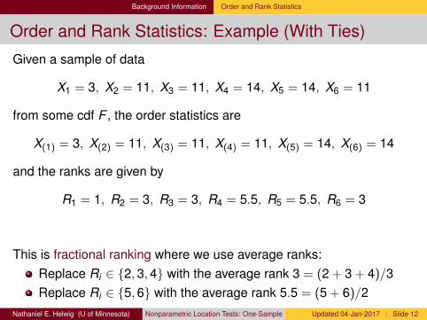
Given a sample of data
X1 = 3, X2 = 11, X3 = 11, X4 = 14, X5 = 14, X6 = 11
from some cdf F , the order statistics are
X(1) = 3, X(2) = 11, X(3) = 11, X(4) = 11, X(5) = 14, X(6) = 14
and the ranks are given by
R1 = 1, R2 = 3, R3 = 3, R4 = 5.5, R5 = 5.5, R6 = 3
This is fractional ranking where we use average ranks:Replace Ri ∈ {2,3,4} with the average rank 3 = (2 + 3 + 4)/3Replace Ri ∈ {5,6} with the average rank 5.5 = (5 + 6)/2
Nathaniel E. Helwig (U of Minnesota) Nonparametric Location Tests: One-Sample Updated 04-Jan-2017 : Slide 12

Background Information Order and Rank Statistics
Order and Rank Statistics: Examples (in R)
Revisit example with no ties:> x = c(3,12,11,18,14,10)> sort(x)[1] 3 10 11 12 14 18> rank(x)[1] 1 4 3 6 5 2
Revisit example with ties:> x = c(3,11,11,14,14,11)> sort(x)[1] 3 11 11 11 14 14> rank(x)[1] 1.0 3.0 3.0 5.5 5.5 3.0
Nathaniel E. Helwig (U of Minnesota) Nonparametric Location Tests: One-Sample Updated 04-Jan-2017 : Slide 13

Background Information Order and Rank Statistics
Summation of Integers (Carl Gauss)
Carl Friedrich Gauss was a German mathematician who madeamazing contributions to all areas of mathematics (including statistics).
According to legend, when Carl was in primary school (about 8 y/o) theteacher asked the class to sum together all integers from 1 to 100.
This was supposed to occupy the students for several hours
After a few seconds, Carl wrote down the correct answer of 5050!Carl noticed that 1 + 100 = 101, 2 + 99 = 101, 3 + 98 = 101, etc.There are 50 pairs that sum to 101 =⇒
∑100i=1 i = 5050
Nathaniel E. Helwig (U of Minnesota) Nonparametric Location Tests: One-Sample Updated 04-Jan-2017 : Slide 14
Background Information Order and Rank Statistics
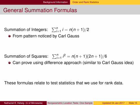
General Summation Formulas
Summation of Integers:∑n
i=1 i = n(n + 1)/2From pattern noticed by Carl Gauss
Summation of Squares:∑n
i=1 i2 = n(n + 1)(2n + 1)/6Can prove using difference approach (similar to Carl Gauss idea)
These formulas relate to test statistics that we use for rank data.
Nathaniel E. Helwig (U of Minnesota) Nonparametric Location Tests: One-Sample Updated 04-Jan-2017 : Slide 15

Background Information One-Sample Problem
Problem(s) of Interest
For the one-sample location problem, we could have:Paired-replicates data: (Xi ,Yi) are independent samplesOne-sample data: Zi are independent samples
We want to make inference about:Paired-replicates data: difference in location (treatment effect)One-sample data: single population’s location
Nathaniel E. Helwig (U of Minnesota) Nonparametric Location Tests: One-Sample Updated 04-Jan-2017 : Slide 16

Background Information One-Sample Problem
Typical Assumptions
Independence assumption:Paired-replicates data: Zi = Yi − Xi are independent samplesOne-sample data: Zi are independent samples
Symmetry assumption:Paired-replicates data: Zi ∼ Fi which is continuous and symmetricaround θ (common median)One-sample data: Zi ∼ Fi which is continuous and symmetricaround θ (common median)
Nathaniel E. Helwig (U of Minnesota) Nonparametric Location Tests: One-Sample Updated 04-Jan-2017 : Slide 17

Wilcoxon’s Signed Rank Test
Wilcoxon’s Signed Rank Test
Nathaniel E. Helwig (U of Minnesota) Nonparametric Location Tests: One-Sample Updated 04-Jan-2017 : Slide 18

Wilcoxon’s Signed Rank Test Overview
Assumptions and Hypothesis
Assumes both independence and symmetry.
The null hypothesis about θ (common median) is
H0 : θ = θ0
and we could have one of three alternative hypotheses:One-Sided Upper-Tail: H1 : θ > θ0
One-Sided Lower-Tail: H1 : θ < θ0
Two-Sided: H1 : θ 6= θ0
Nathaniel E. Helwig (U of Minnesota) Nonparametric Location Tests: One-Sample Updated 04-Jan-2017 : Slide 19
Wilcoxon’s Signed Rank Test Hypothesis Testing
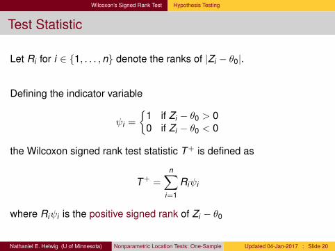
Test Statistic
Let Ri for i ∈ {1, . . . ,n} denote the ranks of |Zi − θ0|.
Defining the indicator variable
ψi =
{1 if Zi − θ0 > 00 if Zi − θ0 < 0
the Wilcoxon signed rank test statistic T+ is defined as
T+ =n∑
i=1
Riψi
where Riψi is the positive signed rank of Zi − θ0
Nathaniel E. Helwig (U of Minnesota) Nonparametric Location Tests: One-Sample Updated 04-Jan-2017 : Slide 20

Wilcoxon’s Signed Rank Test Hypothesis Testing
Distribution of Test Statistic under H0
Assume no ties, let B denote the number of Zi − θ0 values that aregreater than 0, and let r1 < r2 < · · · < rB denote the (ordered) ranks ofthe positive Zi − θ0 values
Note that T+ =∑B
i=1 ri
Under H0 : θ = θ0 we have that Zi − θ0 ∼ Fi , which is continuous andsymmetric around 0.
All 2n possible outcomes for (r1, r2, . . . , rB) occur with equal probability.For given n, form all 2n possible outcomes with corresponding T+
Each outcome has probability 12n under H0
Nathaniel E. Helwig (U of Minnesota) Nonparametric Location Tests: One-Sample Updated 04-Jan-2017 : Slide 21

Wilcoxon’s Signed Rank Test Hypothesis Testing
Null Distribution Example
Suppose we have n = 3 observations (Z1,Z2,Z3) with no ties.
The 23 = 8 possible outcomes for (r1, r2, . . . , rB) areB (r1, r2, . . . , rB) T+ =
∑Bi=1 ri Probability under H0
0 0 1/81 r1 = 1 1 1/81 r1 = 2 2 1/81 r1 = 3 3 1/82 r1 = 1, r2 = 2 3 1/82 r1 = 1, r2 = 3 4 1/82 r1 = 2, r2 = 3 5 1/83 r1 = 1, r2 = 2, r3 = 3 6 1/8
Example probability calculation: P(T+ < 2) =∑1
i=0 P(T+ = i) = 0.25
Nathaniel E. Helwig (U of Minnesota) Nonparametric Location Tests: One-Sample Updated 04-Jan-2017 : Slide 22

Wilcoxon’s Signed Rank Test Hypothesis Testing
Hypothesis Testing
One-Sided Upper Tail Test:H0 : θ = θ0 versus H1 : θ > θ0
Reject H0 if T+ ≥ tα where P(T+ > tα) = α
One-Sided Lower Tail Test:H0 : θ = θ0 versus H1 : θ < θ0
Reject H0 if T+ ≤ n(n+1)2 − tα
Two-Sided Test:H0 : θ = θ0 versus H1 : θ 6= θ0
Reject H0 if T+ ≥ tα/2 or T+ ≤ n(n+1)2 − tα/2
Nathaniel E. Helwig (U of Minnesota) Nonparametric Location Tests: One-Sample Updated 04-Jan-2017 : Slide 23

Wilcoxon’s Signed Rank Test Hypothesis Testing
Large Sample Approximation
Under H0, the expected value and variance of T+ are
E(T+) = n(n+1)4
V (T+) = n(n+1)(2n+1)24
We can create a standardized test statistic T ∗ of the form
T ∗ =T+ − E(T+)√
V (T+)
which asymptotically follows a N(0,1) distribution.
Nathaniel E. Helwig (U of Minnesota) Nonparametric Location Tests: One-Sample Updated 04-Jan-2017 : Slide 24

Wilcoxon’s Signed Rank Test Hypothesis Testing
Derivation of Large Sample Approximation
Note that we have T+ =∑n
i=1 Ui whereUi = Riψi are independent variables for i = 1, . . . ,nP(Ui = i) = P(Ui = 0) = 1/2
Using the independence of the Ui variables we haveE(T+) =
∑ni=1 E(Ui)
V (T+) =∑n
i=1 V (Ui)
Using the distribution of Ui we have
E(Ui) = i 12 + 01
2 = i2 =⇒ E(T+) = 1
2∑n
i=1 i = n(n+1)4
V (Ui) = E(U2i )− [E(Ui)]2 = i2
2 −i24 = i2
4 =⇒V (T+) = 1
4∑n
i=1 i2 = n(n+1)(2n+1)24
Nathaniel E. Helwig (U of Minnesota) Nonparametric Location Tests: One-Sample Updated 04-Jan-2017 : Slide 25

Wilcoxon’s Signed Rank Test Hypothesis Testing
Handling Zeros and Ties
If Zi = θ0, then discard Zi and redefine n as the number ofobservations that do not equal θ0.
If Zi = Zj for two (non-zero) observations, then use the averageranking procedure to handle ties.
T+ is calculated in same fashion (using average ranks)No longer an exact level α testNeed to adjust variance term for large sample approximation
Nathaniel E. Helwig (U of Minnesota) Nonparametric Location Tests: One-Sample Updated 04-Jan-2017 : Slide 26

Wilcoxon’s Signed Rank Test Hypothesis Testing
Example 3.1: Description
Hamilton Depression Scale Factor IV measures suicidal tendencies.Higher scores mean more suicidal tendencies
Nine psychiatric patients were treated with a tranquilizer drug.
X and Y are pre- and post-treatment Hamilton Depression ScaleFactor IV scores
Want to test if the tranquilizer significantly reduced suicidal tendenciesH0 : θ = 0 versus H1 : θ < 0.θ is median of Z = Y − X
Nathaniel E. Helwig (U of Minnesota) Nonparametric Location Tests: One-Sample Updated 04-Jan-2017 : Slide 27

Wilcoxon’s Signed Rank Test Hypothesis Testing
Example 3.1: Data
Nonparametric Statistical Methods, 3rd Ed. (Hollander et al., 2014)
Table 3.1 The Hamilton Depression Scale Factor IV ValuesPatient i Xi Yi
1 1.83 0.8782 0.50 0.6473 1.62 0.5984 2.48 2.0505 1.68 1.0606 1.88 1.2907 1.55 1.0608 3.06 3.1409 1.30 1.290
Source: D. S. Salsburg (1970).
Nathaniel E. Helwig (U of Minnesota) Nonparametric Location Tests: One-Sample Updated 04-Jan-2017 : Slide 28
Wilcoxon’s Signed Rank Test Hypothesis Testing
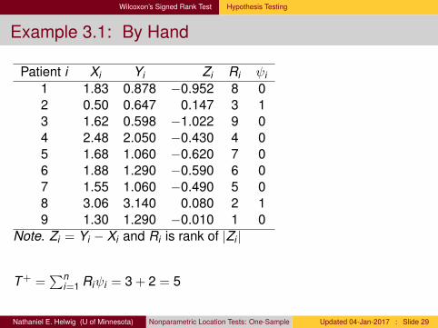
Example 3.1: By Hand
Patient i Xi Yi Zi Ri ψi1 1.83 0.878 −0.952 8 02 0.50 0.647 0.147 3 13 1.62 0.598 −1.022 9 04 2.48 2.050 −0.430 4 05 1.68 1.060 −0.620 7 06 1.88 1.290 −0.590 6 07 1.55 1.060 −0.490 5 08 3.06 3.140 0.080 2 19 1.30 1.290 −0.010 1 0
Note. Zi = Yi − Xi and Ri is rank of |Zi |
T+ =∑n
i=1 Riψi = 3 + 2 = 5
Nathaniel E. Helwig (U of Minnesota) Nonparametric Location Tests: One-Sample Updated 04-Jan-2017 : Slide 29

Wilcoxon’s Signed Rank Test Hypothesis Testing
Example 3.1: Using R
> pre = c(1.83,0.50,1.62,2.48,1.68,1.88,1.55,3.06,1.30)> post = c(0.878,0.647,0.598,2.050,1.060,1.290,1.060,3.140,1.290)> z = post - pre> wilcox.test(z,alternative="less")
Wilcoxon signed rank test
data: zV = 5, p-value = 0.01953alternative hypothesis: true location is less than 0
> wilcox.test(post,pre,alternative="less",paired=TRUE)
Wilcoxon signed rank test
data: post and preV = 5, p-value = 0.01953alternative hypothesis: true location shift is less than 0
Nathaniel E. Helwig (U of Minnesota) Nonparametric Location Tests: One-Sample Updated 04-Jan-2017 : Slide 30

Wilcoxon’s Signed Rank Test Estimating Location
An Estimator of θ
To estimate the median (or median difference) θ, first form theM = n(n + 1)/2 average values
Wij = (Zi + Zj)/2
for i ≤ j = 1, . . . ,n, which are known as Walsh averages.
The estimate of θ corresponding to Wilcoxon’s signed rank test is
θ = median(Wij ; i ≤ j = 1, . . . ,n)
which is the median of the Walsh averages.
Motivation: make mean of Zi − θ as close as possible to n(n + 1)/4.
Nathaniel E. Helwig (U of Minnesota) Nonparametric Location Tests: One-Sample Updated 04-Jan-2017 : Slide 31

Wilcoxon’s Signed Rank Test Confidence Intervals
Symmetric Two-Sided Confidence Interval for θ
Define the following termsM = n(n + 1)/2 is the number of Walsh averagesW (1) ≤W (2) ≤ · · · ≤W (M) are the ordered Walsh averagestα/2 is the critical value such that P(T+ > tα/2) = α/2 under H0
Cα = M + 1− tα/2 is the transformed critical value
A symmetric (1− α)100% confidence interval for θ is given by
θL = W (Cα)
θU = W (M+1−Cα) = W (tα/2)
Nathaniel E. Helwig (U of Minnesota) Nonparametric Location Tests: One-Sample Updated 04-Jan-2017 : Slide 32

Wilcoxon’s Signed Rank Test Confidence Intervals
One-Sided Confidence Intervals for θ
Define the following additional termstα is the critical value such that P(T+ > tα) = α under H0
C∗α = M + 1− tα transformed critical value
An asymmetric (1− α)100% upper confidence bound for θ is
θL = −∞θU = W (M+1−C∗
α) = W (tα)
An asymmetric (1− α)100% lower confidence bound for θ is
θL = W (C∗α)
θU =∞
Nathaniel E. Helwig (U of Minnesota) Nonparametric Location Tests: One-Sample Updated 04-Jan-2017 : Slide 33

Wilcoxon’s Signed Rank Test Confidence Intervals
Example 3.1: Estimate θ
Get W (1) ≤W (2) ≤ · · · ≤W (M) and θ for previous example:
> require(NSM3) # use install.packages("NSM3") to get NSM3> owa(pre,post)$owa[1] -1.0220 -0.9870 -0.9520 -0.8210 -0.8060 -0.7860 -0.7710[8] -0.7560 -0.7260 -0.7210 -0.6910 -0.6200 -0.6050 -0.5900
[15] -0.5550 -0.5400 -0.5250 -0.5160 -0.5100 -0.4900 -0.4810[22] -0.4710 -0.4600 -0.4375 -0.4360 -0.4300 -0.4025 -0.3150[29] -0.3000 -0.2700 -0.2550 -0.2500 -0.2365 -0.2215 -0.2200[36] -0.2050 -0.1750 -0.1715 -0.1415 -0.0100 0.0350 0.0685[43] 0.0800 0.1135 0.1470
$h.l[1] -0.46
Nathaniel E. Helwig (U of Minnesota) Nonparametric Location Tests: One-Sample Updated 04-Jan-2017 : Slide 34

Wilcoxon’s Signed Rank Test Confidence Intervals
Example 3.1: Confidence Interval for θ
> wilcox.test(z,alternative="less",conf.int=TRUE)
Wilcoxon signed rank test
data: zV = 5, p-value = 0.01953
alternative hypothesis: true location is less than 095 percent confidence interval:
-Inf -0.175sample estimates:(pseudo)median
-0.46
Nathaniel E. Helwig (U of Minnesota) Nonparametric Location Tests: One-Sample Updated 04-Jan-2017 : Slide 35

Fisher’s Sign Test
Fisher’s Sign Test
Nathaniel E. Helwig (U of Minnesota) Nonparametric Location Tests: One-Sample Updated 04-Jan-2017 : Slide 36

Fisher’s Sign Test Overview
Assumptions and Hypothesis
Assumes only independence (no symmetry assumption).
The null hypothesis about θ (common median) is
H0 : θ = θ0
and we could have one of three alternative hypotheses:One-Sided Upper-Tail: H1 : θ > θ0
One-Sided Lower-Tail: H1 : θ < θ0
Two-Sided: H1 : θ 6= θ0
Nathaniel E. Helwig (U of Minnesota) Nonparametric Location Tests: One-Sample Updated 04-Jan-2017 : Slide 37

Fisher’s Sign Test Hypothesis Testing
Test Statistic
Defining the indicator variable
ψi =
{1 if Zi − θ0 > 00 if Zi − θ0 < 0
the sign test statistic B is defined as
B =n∑
i=1
ψi
which is the number of positive Zi − θ0 values.
Nathaniel E. Helwig (U of Minnesota) Nonparametric Location Tests: One-Sample Updated 04-Jan-2017 : Slide 38

Fisher’s Sign Test Hypothesis Testing
Distribution of Test Statistic under H0
If θ0 is the true median, ψi has a 50% chance of taking each value:P(ψ = 0|θ = θ0) = P(ψ = 1|θ = θ0) = 1/2
Thus, the sign statistic follows a binomial distribution under H0
B ∼ Binom(n,1/2)
Nathaniel E. Helwig (U of Minnesota) Nonparametric Location Tests: One-Sample Updated 04-Jan-2017 : Slide 39
Fisher’s Sign Test Hypothesis Testing
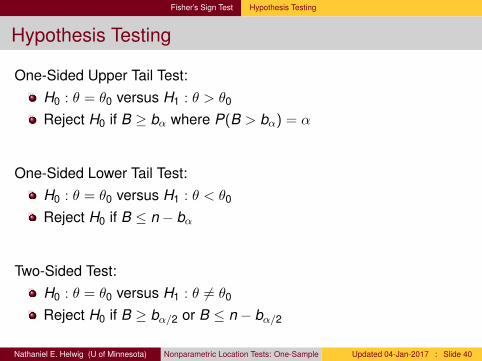
Hypothesis Testing
One-Sided Upper Tail Test:H0 : θ = θ0 versus H1 : θ > θ0
Reject H0 if B ≥ bα where P(B > bα) = α
One-Sided Lower Tail Test:H0 : θ = θ0 versus H1 : θ < θ0
Reject H0 if B ≤ n − bα
Two-Sided Test:H0 : θ = θ0 versus H1 : θ 6= θ0
Reject H0 if B ≥ bα/2 or B ≤ n − bα/2
Nathaniel E. Helwig (U of Minnesota) Nonparametric Location Tests: One-Sample Updated 04-Jan-2017 : Slide 40

Fisher’s Sign Test Hypothesis Testing
Large Sample Approximation
Under H0, B ∼ Binom(n,1/2) so the expected value and variance areE(B) = np = n
2
V (B) = np(1− p) = n4
We can create a standardized test statistic B∗ of the form
B∗ =B − E(B)√
V (B)
which asymptotically follows a N(0,1) distribution.
Nathaniel E. Helwig (U of Minnesota) Nonparametric Location Tests: One-Sample Updated 04-Jan-2017 : Slide 41

Fisher’s Sign Test Hypothesis Testing
Example 3.1: Revisited (By Hand)
Patient i Xi Yi Zi ψi1 1.83 0.878 −0.952 02 0.50 0.647 0.147 13 1.62 0.598 −1.022 04 2.48 2.050 −0.430 05 1.68 1.060 −0.620 06 1.88 1.290 −0.590 07 1.55 1.060 −0.490 08 3.06 3.140 0.080 19 1.30 1.290 −0.010 0
B =∑n
i=1 ψi = 2 and p-value = P(B < 2|H0 is true) = 0.0898> pbinom(2,9,1/2)[1] 0.08984375
Nathaniel E. Helwig (U of Minnesota) Nonparametric Location Tests: One-Sample Updated 04-Jan-2017 : Slide 42

Fisher’s Sign Test Hypothesis Testing
Example 3.1: Revisited (Using R, one-sample)
> library(BSDA)> z = post - pre> SIGN.test(z,alternative="less")
One-sample Sign-Test
data: zs = 2, p-value = 0.08984alternative hypothesis: true median is less than 095 percent confidence interval:-Inf 0.041
sample estimates:median of x
-0.49
Conf.Level L.E.pt U.E.ptLower Achieved CI 0.9102 -Inf -0.010Interpolated CI 0.9500 -Inf 0.041Upper Achieved CI 0.9805 -Inf 0.080
Nathaniel E. Helwig (U of Minnesota) Nonparametric Location Tests: One-Sample Updated 04-Jan-2017 : Slide 43

Fisher’s Sign Test Hypothesis Testing
Example 3.1: Revisited (Using R, paired-samples)
> library(BSDA)> SIGN.test(post,pre,alternative="less")
Dependent-samples Sign-Test
data: post and preS = 2, p-value = 0.08984alternative hypothesis: true median difference is less than 095 percent confidence interval:-Inf 0.041
sample estimates:median of x-y
-0.49
Conf.Level L.E.pt U.E.ptLower Achieved CI 0.9102 -Inf -0.010Interpolated CI 0.9500 -Inf 0.041Upper Achieved CI 0.9805 -Inf 0.080
Nathaniel E. Helwig (U of Minnesota) Nonparametric Location Tests: One-Sample Updated 04-Jan-2017 : Slide 44

Fisher’s Sign Test Estimating Location
A Different Estimator of θ
To estimate the median (or median difference) θ, calculate
θ = median(Zi ; i = 1, . . . ,n)
which is the median of observed sample (or paired differences).> median(z)[1] -0.49
Motivation: make mean of Zi − θ as close as possible to n/2.
Nathaniel E. Helwig (U of Minnesota) Nonparametric Location Tests: One-Sample Updated 04-Jan-2017 : Slide 45

Fisher’s Sign Test Confidence Intervals
Symmetric Two-Sided Confidence Interval for θ
Define the following termsbα/2 is the critical value such that P(B > bα/2) = α/2 under H0
Cα = n + 1− bα/2 is the transformed critical value
A symmetric (1− α)100% confidence interval for θ is given by
θL = Z (Cα)
θU = Z (n+1−Cα) = Z (bα/2)
where Z (i) is the i-th order statistic of the sample {Zi}ni=1.
Nathaniel E. Helwig (U of Minnesota) Nonparametric Location Tests: One-Sample Updated 04-Jan-2017 : Slide 46

Fisher’s Sign Test Confidence Intervals
One-Sided Confidence Intervals for θ
Define the following additional termsbα is the critical value such that P(B > bα) = α under H0
C∗α = n + 1− bα transformed critical value
An asymmetric (1− α)100% upper confidence bound for θ is
θL = −∞θU = Z (n+1−C∗
α) = Z (bα)
An asymmetric (1− α)100% lower confidence bound for θ is
θL = Z (C∗α)
θU =∞
Nathaniel E. Helwig (U of Minnesota) Nonparametric Location Tests: One-Sample Updated 04-Jan-2017 : Slide 47

Fisher’s Sign Test Confidence Intervals
Example 3.1: Revisited Confidence Interval for θ
> zs = sort(z)> zs[1] -1.022 -0.952 -0.620 -0.590 -0.490[6] -0.430 -0.010 0.080 0.147> round(pbinom(0:9,9,1/2),4)[1] 0.0020 0.0195 0.0898 0.2539 0.5000[6] 0.7461 0.9102 0.9805 0.9980 1.0000> zs[7:8]
[1] -0.01 0.08> zs[7]+(zs[8]-zs[7])*(0.95-0.9102)/(0.9805-0.9102)[1] 0.04095306
The asymmetric 95% upper confidence bound is (−∞,0.041).
Nathaniel E. Helwig (U of Minnesota) Nonparametric Location Tests: One-Sample Updated 04-Jan-2017 : Slide 48

Some Considerations
Some Considerations
Nathaniel E. Helwig (U of Minnesota) Nonparametric Location Tests: One-Sample Updated 04-Jan-2017 : Slide 49

Some Considerations Choosing a Location Test
Which Location Test Should You Choose?
Answer depends on your data and what assumptions you are willing tomake about the population distribution.
If observed data are normally distributed, then. . .t-test is most powerful testWilcoxon’s signed rank test is slightly less powerful than t test(4.5% efficiency loss)Fisher’s sign test is less powerful than others(36.3% efficiency loss compared to t test)
If observed data are NOT normally distributed, then. . .Signed rank test is typically as or more efficient than t testSign test should be preferred if data population is asymmetric
Nathaniel E. Helwig (U of Minnesota) Nonparametric Location Tests: One-Sample Updated 04-Jan-2017 : Slide 50

Some Considerations Univariate Symmetry Test
Assumptions and Hypotheses
Assumes ziiid∼ F where θ is the median of F , i.e., F (θ) = 1/2
The null hypothesis is that F is symmetric around θ, i.e.,
H0 : F (θ − b) + F (θ + b) = 1 ∀b
and we could have one of three alternative hypotheses:One-Sided Left-Skew: H1 : F (θ + b) ≥ 1− F (θ − b) ∀b > 0One-Sided Right-Skew: H1 : F (θ + b) ≤ 1− F (θ − b) ∀b > 0Two-Sided: F (θ − b) + F (θ + b) 6= 1 for any b
Nathaniel E. Helwig (U of Minnesota) Nonparametric Location Tests: One-Sample Updated 04-Jan-2017 : Slide 51

Some Considerations Univariate Symmetry Test
Test Statistic
For every triple of observations (Zi ,Zj ,Zk ), 1 ≤ i < j < k ≤ n, define
f ∗(Zi ,Zj ,Zk ) = sign(Zi +Zj−2Zk )+sign(Zi +Zk−2Zj)+sign(Zj +Zk−2Zi)
and note that there are n(n− 1)(n− 2)/6 distinct triples in the sample.(Zi ,Zj ,Zk ) is a left triple (skewed to left) if f ∗(Zi ,Zj ,Zk ) = −1(Zi ,Zj ,Zk ) is a right triple (skewed to right) if f ∗(Zi ,Zj ,Zk ) = 1If f ∗(Zi ,Zj ,Zk ) = 0, then (Zi ,Zj ,Zk ) is neither left nor right
Define the unstandardized test statistic
T =∑
1≤i<j<k≤n
f ∗(Zi ,Zj ,Zk )
= {# of right triples} − {# of left triples}
Nathaniel E. Helwig (U of Minnesota) Nonparametric Location Tests: One-Sample Updated 04-Jan-2017 : Slide 52

Some Considerations Univariate Symmetry Test
Test Statistic (continued)
Define the standardized test statistic
V = T/σ asy∼ N(0,1)
where the variance estimate is given by
σ2 =(n − 3)(n − 4)
(n − 1)(n − 2)
n∑t=1
B2t +
(n − 3)
(n − 4)
n−1∑s=1
n∑t=s+1
B2s,t
+n(n − 1)(n − 2)
6−[1− (n − 3)(n − 4)(n − 5)
n(n − 1)(n − 2)
]T 2
and the Bt and Bst terms are defined as
Bt = {# right triples involving Zt} − {# left triples involving Zt}Bst = {# right triples involving Zs,Zt} − {# left triples involving Zs,Zt}
Nathaniel E. Helwig (U of Minnesota) Nonparametric Location Tests: One-Sample Updated 04-Jan-2017 : Slide 53

Some Considerations Univariate Symmetry Test
Hypothesis Testing
One-Sided Left-Skew Test:H0 : F is symmetric versus H1 : F is left-skewedReject H0 if V ≤ −Zα where P(Z > Zα) = α
One-Sided Right-Skew Test:H0 : F is symmetric versus H1 : F is right-skewedReject H0 if V ≥ Zα
Two-Sided Test:H0 : F is symmetric versus H1 : F is not symmetricReject H0 if |V | ≥ Zα/2
Nathaniel E. Helwig (U of Minnesota) Nonparametric Location Tests: One-Sample Updated 04-Jan-2017 : Slide 54

Some Considerations Univariate Symmetry Test
Example 1: Symmetric
> set.seed(1)> x = rnorm(50)> hist(x)> require(NSM3)> test = RFPW(x)> c(test$obs.stat, test$p.val)[1] -1.4572415 0.1450497
# two-sided> 2*(1 - pnorm(abs(test$obs.stat)))[1] 0.1450497# left-skew> pnorm(test$obs.stat)[1] 0.07252486# right-skew> 1 - pnorm(test$obs.stat)[1] 0.9274751
Histogram of x
x
Fre
quen
cy
−2 −1 0 1 2
02
46
810
1214
Nathaniel E. Helwig (U of Minnesota) Nonparametric Location Tests: One-Sample Updated 04-Jan-2017 : Slide 55

Some Considerations Univariate Symmetry Test
Example 2: Asymmetric
> set.seed(1)> x = rchisq(50,df=3)> hist(x)> require(NSM3)> test = RFPW(x)> c(test$obs.stat, test$p.val)[1] 1.70708892 0.08780553
# two-sided> 2*(1 - pnorm(abs(test$obs.stat)))[1] 0.08780553# left-skew> pnorm(test$obs.stat)[1] 0.9560972# right-skew> 1 - pnorm(test$obs.stat)[1] 0.04390276
Histogram of x
x
Fre
quen
cy
0 1 2 3 4 5 6
02
46
810
1214
Nathaniel E. Helwig (U of Minnesota) Nonparametric Location Tests: One-Sample Updated 04-Jan-2017 : Slide 56

Some Considerations Bivariate Symmetry Test
Exchangeability
Components of a random vector (X ,Y ) are exchangeable if thevectors (X ,Y ) and (Y ,X ) have the same distribution.
Permuting components does not change distributionImplies FX ≡ FY and FX |Y ≡ FY |X and FZ ≡ F−Z with Z = Y − XFZ ≡ F−Z implies that FZ is symmetric about 0
More generally, if components of (X + θ,Y ) are exchangeable, then
Z − θ = Y − (X + θ)
has the same distribution as
θ − Z = (X + θ)− Y
implies that FZ is symmetric about θNathaniel E. Helwig (U of Minnesota) Nonparametric Location Tests: One-Sample Updated 04-Jan-2017 : Slide 57

Some Considerations Bivariate Symmetry Test
Assumptions and Hypotheses
Assumes (xi , yi)iid∼ F (x , y) where F is some bivariate distribution.
The null hypothesis is that F is exchangeable, i.e.,
H0 : F (x , y) = F (y , x) ∀x , y
and there is only one possible alternative hypothesis
H1 : F (x , y) 6= F (y , x) for some x , y
Nathaniel E. Helwig (U of Minnesota) Nonparametric Location Tests: One-Sample Updated 04-Jan-2017 : Slide 58

Some Considerations Bivariate Symmetry Test
Test Statistic
For each pair (xi , yi) let ai = min(xi , yi) and bi = max(xi , yi), and define
ri =
{1, if xi = ai < bi = yi0, if xi = bi ≥ ai = yi
so that ri = 1 if xi < yi and ri = 0 otherwise.
Next, define the n2 values dij , for i , j = 1, . . . ,n, as
dij =
{1, if aj < bi ≤ bj and ai ≤ aj0, otherwise
Nathaniel E. Helwig (U of Minnesota) Nonparametric Location Tests: One-Sample Updated 04-Jan-2017 : Slide 59

Some Considerations Bivariate Symmetry Test
Test Statistic (continued)
For each j = 1, . . . ,n calculate the signed summation of dij as
Tj =n∑
i=1
sidij
where si = 2ri − 1. Note that si = 1 if ri = 1 and si = −1 if ri = 0.
Finally, calculate the observed test statistic
Aobs =1n2
n∑j=1
T 2j
Nathaniel E. Helwig (U of Minnesota) Nonparametric Location Tests: One-Sample Updated 04-Jan-2017 : Slide 60

Some Considerations Bivariate Symmetry Test
Distribution of Test Statistic under H0
In addition to observed (r1, . . . , rn), there are 2n−1 other possibilities.ri can be 0 or 1, so there are 2n total configurationsEach configuration is equally likely under H0
Let A(1) ≤ A(2) ≤ · · · ≤ A(2n) denote the 2n values of the test statistic.Need to form all possible A(k) values for make null distributionNote that dij is same for all A(k) values (by definition of dij )
Nathaniel E. Helwig (U of Minnesota) Nonparametric Location Tests: One-Sample Updated 04-Jan-2017 : Slide 61

Some Considerations Bivariate Symmetry Test
Hypothesis Testing
Two-Sided Test:H0 : F is exchangeable versus H1 : F is not exchangeableReject H0 if Aobs > A(m) where m = 2n − b2nαc
If you are unlucky and Aobs = A(m), use a randomized decision.Reject H0 with probability q = 2nα−M1
M2
M1 =∑2n
k=1 1{A(k)>A(m)} is the # of A(k) values greater than A(m)
M2 =∑2n
k=1 1{A(k)=A(m)} is the # of A(k) values equal to A(m)
Nathaniel E. Helwig (U of Minnesota) Nonparametric Location Tests: One-Sample Updated 04-Jan-2017 : Slide 62

Some Considerations Bivariate Symmetry Test
Example 3.1: Exchangeability Test
> pre = c(1.83,0.50,1.62,2.48,1.68,1.88,1.55,3.06,1.30)> post = c(0.878,0.647,0.598,2.050,1.060,1.290,1.060,3.140,1.290)> require(NSM3)> HollBivSym(pre,post)[1] 0.6666667> set.seed(1)> pHollBivSym(pre,post)Number of X values: 9 Number of Y values: 9Hollander A Statistic: 0.6667Monte Carlo (Using 10000 Iterations) upper-tail probability: 0.0321
Nathaniel E. Helwig (U of Minnesota) Nonparametric Location Tests: One-Sample Updated 04-Jan-2017 : Slide 63