Embed Size (px)
Citation preview

Nonrivalry and the Economics of Data
Charles I. Jones Christopher Tonetti∗
Stanford GSB and NBER Stanford GSB and NBER
August 29, 2019 — Version 1.0
Abstract
Data is nonrival: a person’s location history, medical records, and driving data
can be used by any number of firms simultaneously. Nonrivalry leads to increasing
returns and implies an important role for market structure and property rights.
Who should own data? What restrictions should apply to the use of data? We
show that in equilibrium, firms may not adequately respect the privacy of consu-
mers. But nonrivalry leads to other consequences that are less obvious. Because of
nonrivalry, there may be large social gains to data being used broadly across firms,
even in the presence of privacy considerations. Fearing creative destruction, firms
may choose to hoard data they own, leading to the inefficient use of nonrival data.
Instead, giving the data property rights to consumers can generate allocations that
are close to optimal. Consumers balance their concerns for privacy against the
economic gains that come from selling data to all interested parties.
∗We are grateful to Dan Bjorkegren, Yan Carriere-Swallow, V.V. Chari, Sebastian Di Tella, Joshua Gans,Avi Goldfarb, Mike Golosov, Vikram Haksar, Ben Hebert, Pete Klenow, Hannes Malmberg, Aleh Tsyvinski,Hal Varian, Laura Veldkamp, and Heidi Williams for helpful comments and to Andres Yany for excellentresearch assistance.

NONRIVALRY AND THE ECONOMICS OF DATA 1
1 Introduction
In recent years, the importance of data in the economy has become increasingly appa-
rent. More powerful computers, the growth of networks, and advances such as machine
learning have led to an explosion in the usefulness of data. Examples include self-
driving cars, real-time language translation, medical diagnoses, product recommen-
dations, and social networks.
This paper develops a theoretical framework to study the economics of data. We
are particularly interested in how different property rights for data determine its use
in the economy, and thus affect output, privacy, and consumer welfare. The starting
point for our analysis is the observation that data is nonrival. That is, at a technological
level, data is infinitely usable. Most goods in economics are rival: if a person consumes
a kilogram of rice or an hour of an accountant’s time, some resource with a positive
opportunity cost is used up. In contrast, existing data can be used by any number of
firms or people simultaneously, without being diminished. Consider a collection of a
million labeled images, the human genome, the U.S. Census, or the data generated by
10,000 cars driving 10,000 miles. Any number of firms, people, or machine learning
algorithms can use this data simultaneously without reducing the amount of data avai-
lable to anyone else.
The key finding in our paper is that policies related to data have important econo-
mic consequences. When firms own data, they may not adequately respect the pri-
vacy of consumers. But nonrivalry leads to other consequences that are less obvious.
Because data is nonrival, there are potentially large gains to data being used broadly.
Markets for data provide financial incentives that promote broader use, but if selling
data increases the rate of creative destruction, firms may hoard data in ways that are
socially inefficient.
An analogy may be helpful. Because capital is rival, each firm must have its own
building, each worker needs her own desk and computer, and each warehouse needs
its own collection of forklifts. But if capital were nonrival, it would be as if every auto
worker in the economy could use the entire industry’s stock of capital at the same time.
Clearly this would produce tremendous economic gains. This is what is possible with
data. Obviously there may be incentive reasons why it is inefficient to have all data used
by all firms. But the equilibrium in which firms own data and sharply limit its use by
2 JONES AND TONETTI
other firms may also be inefficient. Our numerical examples suggest that these costs
can be large.
Another allocation we consider is one in which a government — perhaps out of
concern for privacy — sharply limits the use of consumer data by firms. While this
policy succeeds in generating privacy gains, it may potentially have an even larger
cost because of the inefficiency that arises from a nonrival input not being used at the
appropriate scale.
Finally, we consider an institutional arrangement in which consumers own the data
associated with their behavior. Consumers then balance their concerns for privacy
against the economic gains that come from selling data to all interested parties. This
equilibrium results in data being used broadly across firms, taking advantage of the
nonrivalry of data. For a broad range of parameter values in our numerical example,
this allocation generates consumption and welfare that are close to optimal.
To put this concretely, suppose doctors use software to help diagnose skin cancer.
An algorithm can be trained using images of potential cancers labeled with pathology
reports and cancer outcomes. Imagine a world in which hospitals own data and each
uses labeled images from all patients in its network to train the algorithm. Now com-
pare that to a situation in which competing algorithms can each use all the images
from all patients in the United States, or even the world. The software based on larger
samples could help doctors everywhere better treat patients and save lives. The gain
to any single hospital from selling its data broadly may not be sufficient to generate
the broad use that is beneficial to society, either because of concerns related to creative
destruction or perhaps because of legal restrictions. Consumers owning their medical
data and selling it to all interested researchers, hospitals, and entrepreneurs may result
in a world closer to the social optimum in which such valuable data is used broadly to
help many.
The remainder of the paper is structured as follows. The introduction continues
with a discussion of how we model data and on the similarities and differences between
data and ideas — another nonrival good — and provides a literature review. Section 2
provides a simple model to demonstrate the link between nonrivalry and scale effects.
Section 3 turns to the full model and presents the economic environment. Section 4
examines the allocation chosen by the social planner. Section 5 turns to a decentralized
NONRIVALRY AND THE ECONOMICS OF DATA 3
equilibrium in which firms own data and shows that it may be privately optimal for a
firm to both overuse its own data and to sharply limit data sales to other firms. Section 6
instead considers an allocation in which consumers own data and, weighing privacy
considerations, sell some of it to multiple firms. Section 7 shows what happens if the
government outlaws the selling of data. Section 8 collects and discusses our main
theoretical results while Section 9 presents a numerical simulation of our model to
illustrate the various forces at work.
1.1 Data versus Ideas
We find it helpful to define information as the set of all economic goods that are nonri-
val. That is, information consists of economic goods that can be entirely represented as
bit strings, i.e., as sequences of ones and zeros. Ideas and data are types of information.
Following Romer (1990), an idea is a piece of information that is a set of instructions for
making an economic good, which may include other ideas. Data denotes the remai-
ning forms of information. It includes things like driving data, medical records, and
location data that are not themselves instructions for making a good but that may still
be useful in the production process, including in producing new ideas. An idea is a
production function whereas data is a factor of production.
Some examples distinguishing data from ideas might be helpful. First, consider a
million images of cats, rainbows, kids, buildings, etc., labeled with their main subject.
Data like this is extremely useful for training machine learning algorithms, but these
labeled images are clearly not themselves ideas, i.e., not blueprints. The same is true of
the hourly heart-rate history of a thousand people or the speech samples of a popula-
tion. It seems obvious at this level that data and ideas are distinct.
Second, consider the efforts to build a self-driving car. The essence is a machine
learning algorithm, which can be thought of as a collection of nonlinear regressions at-
tempting to forecast what actions an expert driver will take given the data from various
sensors including cameras, lidar, GPS, and so on. Data in this example includes both
the collection of sensor readings and the actions taken by expert drivers. The nonli-
near regression estimates a large number of parameters to produce the best possible
forecasts. A successful self-driving car algorithm — a computer program, and hence an
idea — is essentially just the forecasting rules that come from using data to estimate

4 JONES AND TONETTI
the parameters of the nonlinear model. The data and the idea are distinct: the software
algorithm is the idea that is embedded in the self-driving cars of the future; data is an
input used to produce this idea.
Another dimension along which ideas and data can differ is the extent to which they
are excludable. On the one hand, it seems technologically easier to transmit data than
to transmit ideas. Data can be sent at the press of button over the internet, whereas
we invest many resources in education to learn ideas. On the other hand, data can be
encrypted. Engineers change jobs and bring knowledge with them; people move and
communicate causing ideas to diffuse, at least eventually. Data, in contrast, especially
when it is “big,” may be more easily monitored and made to be highly excludable.
The “idea” of machine learning is public, whereas the driving data that is fed into the
machine learning algorithm is kept private; each firm is gathering its own data.
1.2 Relation to the Literature
The “economics of data” is a new but rapidly-growing field. In this paper we provide
a macro perspective. Since we emphasize nonrivalry, there are parallels between how
data appears in our model and how ideas appear in the growth literature. Compared to
the growth literature, the most distinctive features of our model are
1. The use of nonrival goods: our setup features the simultaneous broad use of data
by many firms; in Romer (1990) and Aghion and Howitt (1992) style models, each
firm produces using a single idea.
2. The market for nonrival goods: our setup features markets through which each
firm decides on a quantity of data to buy and sell; in idea-based models, typically
the inventing firm produces itself or sells a single blueprint to a single monopoly
producer.
3. Property rights: in idea-based models, property rights for ideas are always held
by firms; in our setup, comparing consumer versus firm ownership of data is
fundamental.
At the core of our analysis of decentralized equilibria is a market for data. This
feature is related to the market for ideas in Akcigit et al. (2016). In their setup the idea is
used by only one firm at a time and the market helps to allocate the idea to the firm who
NONRIVALRY AND THE ECONOMICS OF DATA 5
could best make use of it. In contrast, our market for data allows multiple firms to use
the nonrival good simultaneously. The literature on patent-licensing would be the clo-
sest to our paper since it studies legal arrangements under which multiple firms can use
a given idea at the same time. From a more micro perspective, see Ali et al. (2019) who
study the sale of nonrival information in a search and matching decentralized market
and emphasize that nonrivalry generates inefficiency due to the under-utilization of
information. Ichihashi (2019) studies competition among data intermediaries. Akcigit
and Liu (2016) show in a growth context how the information that certain research
paths lead to dead ends is socially valuable and how an economy may suffer from an
inefficient duplication of research if this information is not shared across firms.
Given our macroeconomic perspective, we remain silent on many of the interesting
related topics in industrial organization. Varian (2018) provides a general discussion of
the economics of data and machine learning. He emphasizes that data is nonrival and
refers to a common notion that “data is the new oil.” Varian notes that this nonrivalry
means that “data access” may be more important than “data ownership” and sugge-
sts that while markets for data are relatively limited at this point, some types of data
(like maps) are currently licensed by data providers to other firms. Our paper explores
these and other insights in a formal model. Our results suggest that data ownership is
likely to influence data access. In addition to thinking about property rights granted to
firms who can sell their nonrival goods, we consider granting property rights to data
to consumers. The fact that consumer interaction is necessary to create data in our
setup makes the consumers-own-data property right regime a natural consideration,
whereas the growth literature almost exclusively focuses on property rights granted to
firms.
Data as a byproduct of economic activity also has analogues in the information
economics literature. For example, see Veldkamp (2005), Ordonez (2013), Fajgelbaum
et al. (2017), and Bergemann and Bonatti (2019). Arrieta Ibarra, Goff, Jimenez Hernan-
dez, Lanier and Weyl (2018) and Posner and Weyl (2018) emphasize a “data as labor”
perspective: data is a key input to many technology firms, and people may not be
adequately compensated for the data they provide, perhaps because of market power
considerations.
Acquisti, Taylor and Wagman (2016) discuss the economics of privacy and how con-
6 JONES AND TONETTI
sumers value the privacy of their data. In the context of medical records, Miller and
Tucker (2017) find that approaches to privacy that give users control over redisclosure
encourage the spread of genetic testing, consistent with the mechanism that we high-
light in this paper. See Ali et al. (2018) who study consumer disclosure of personal
information to firms and the consequent pricing and welfare implications. Goldfarb
and Tucker (2011) highlight a tradeoff between privacy and the effectiveness of online
advertising. Chiou and Tucker (2017) study how the length of time that search engines
keep their server logs affects the accuracy of their subsequent searches and find little
evidence of a large impact. Abowd and Schmutte (2019) emphasize that privacy isn’t
binary; there is an intensive margin to privacy with a choice of how much data to use.
They propose a differential privacy framework to produce the socially optimal use of
data that respects privacy concerns. Our paper features such an intensive margin of
data use with corresponding tradeoffs.
Farboodi and Veldkamp (2019) is a paper complimentary to ours. We focus on
property rights and how the associated sale and use of nonrival data can affect effi-
ciency. They emphasize that data is information that can be used to reduce forecast
errors, suggesting a production function with bounded returns to data. We suspect that
our main results about the productivity benefits (“level effects”) from the broad use of
nonrival data would survive even with bounded returns; our Cobb-Douglas specifica-
tion is helpful for tractability. Farboodi and Veldkamp (2017) study the implications
of expanding access to data for financial markets. Begenau, Farboodi and Veldkamp
(2017) suggest that access to big data has lowered the cost of capital for large firms
relative to small ones, leading to a rise in firm-size inequality.
Agrawal, Gans and Goldfarb (2018) provide an overview of the economics of ma-
chine learning. Bajari, Chernozhukov, Hortacsu and Suzuki (2018) examine how the
amount of data impacts weekly retail sales forecasts for product categories at Amazon.
They find that forecasts for a given product improve with the square-root of the number
of weeks of data on that product. However, forecasts of sales for a given category do not
seem to improve much as the number of products within the category grows. Azevedo,
Deng, Montiel Olea, Rao and Weyl (2019) suggest that the distribution of outcomes in
A/B testing in internet search may be fat-tailed: rare outcomes can have very high re-
turns. Carriere-Swallow and Haksar (2019) note that credit bureaus are a long-standing
NONRIVALRY AND THE ECONOMICS OF DATA 7
market institution that facilitates the broad use of nonrival data, at least in one context.
Hughes-Cromwick and Coronado (2019) view government data as a public good and
study its value to U.S. businesses.
In order to emphasize the relationship between nonrivalry and scale effects and
to study different property right regimes in a simple environment, our model omits
some interesting features prevalent in the literature on data. In our model, data does
not affects a firm’s ability to discriminate against consumers via price or quantity. For
example, we do not model firms that are able to learn whether the degree to which
individuals are price sensitive or to refuse to sell insurance to people with high health
risks. These considerations are important, so we view our paper as emphasizing an
underappreciated channel relevant to the design of data property rights, but it does
not provide a complete accounting of the pros and cons of the widespread availability
and use of data.
A question that comes up immediately in this paper is why the Coase (1960) theo-
rem does not apply: why does it matter whether firms or consumers own data initially?
With trade and monetary transfers, why isn’t the allocation the same in either case? One
could certainly set up the model so that this would be true. However, to illustrate the
importance of data sharing, we assume that the Coase theorem fails. In particular, we
assume that consumers cannot commit to sell their data to only a single firm. Notice
that this issue arises solely because of nonrivalry: a given apple can only be eaten
once. This lack of commitment serves to illustrate various properties of an economy
with data; similar assumptions are typically made in growth models with knowledge
spillovers and creative destruction. How it plays out in the real world is a distinct
and interesting question, but we simply note that there are many recent episodes in
the news in which firms display a remarkable inability to avoid selling or using data
that they have access to, often at odds with public statements on data-use policy, so
this assumption — in addition to its pedagogical role — may actually have real-world
relevance. Dosis and Sand-Zantman (2019) provide a micro-founded model of the
failure of the Coase theorem in studying the property rights over the use of data. They
emphasize that whether it is better for firms or consumers to own data depends on
the overall value of the data to the firm and on the extent to which consumers can
monetize their data. They do not consider the nonrivalry of data, however. See also
8 JONES AND TONETTI
Chari and Jones (2000) for some of the problems in implementing the Coase theorem
in economies with public goods.
2 A Simple Model
Suppose the economy consists of N varieties. To be concrete, think of self-driving cars
(e.g. Tesla, Uber, Waymo, and so on). Consumption of each variety combines in a CES
fashion to produce a utility aggregate Y , which we also think of as aggregate output.
With symmetry, Y is given by
Y =
(∫ N
0Y
σ−1σ
i di
) σσ−1
= Nσσ−1Yi.
Variety i is produced using labor Li and data Di:
Yi = Dηi Li = Dη
i L/N = Dηi ν
where L is the total amount of labor in the economy, allocated symmetrically across
varieties, and ν ≡ L/N is firm size measured by employment. The nonrival nature of
data means there are constant returns to labor and increasing returns to labor and data
together; this parallels the Romer (1990) insight that the nonrivalry of ideas gives rise to
increasing returns. The parameter η measures the importance of data and the degree
of increasing returns. Intuitively, a given amount of data can be used to train a machine
learning algorithm to help make cars safer. With a little data, this may allow the car to
apply emergency braking when needed. A machine learning algorithm trained on even
more data may be able to drive on highways and in bumper-to-bumper traffic. In other
words, data can be viewed as improving the quality of an idea.
Importantly, a given amount of data trains a machine learning algorithm that can
then be used in 1 car, 1000 cars, or 1 million cars simultaneously; this is the nonrivalry
of the idea that is produced by the data. The nonrivalry of data will make its appea-
rance shortly, when we note that the same data can be used by many different firms to
produce their own trained machine learning algorithms.
Whenever a variety is consumed, it generates one piece of data: each mile driven
NONRIVALRY AND THE ECONOMICS OF DATA 9
generates data that raises the productivity of future trips. Data generated by Tesla cars
is useful to Tesla. But data generated by Uber and Waymo could also potentially be
useful to Tesla. We formalize this as
Di = αxYi + (1− α)Bi
= αxiYi + (1− α)xNYi
= [αx+ (1− α)xN ]Yi (1)
In the first line, Yi is the amount of data generated by Tesla trips, and x is the fraction of
that data that Tesla is allowed to use. Bi is the bundle of data from other varieties that
Tesla gets to use. The parameter αmeasures the importance of Tesla’s own data relative
to the data bundle from other firms.
The second line in this expression uses the fact that Bi ≡ xNYi. The quantity
NYi is the amount of data generated by Uber, Waymo, and the other varieties in the
economy (because variety i is infinitesimal and because firms are symmetric), and x
is the fraction of other firms’ data that Tesla gets to use. Both x and x are endogenous
allocations in our richer model, chosen subject to privacy considerations. For now,
though, we just treat them as parameters. The third line above just factor outs Yi.
Substituting this expression for data back into variety i’s production function gives
Yi = ([αx+ (1− α)xN ]ην)1
1−η .
There is a multiplier associated with data. The more people consume your product,
the more data you have. This raises productivity and generates more output and con-
sumption and hence more data, completing the circle. The sum of this geometric series
is 11−η , which is the key exponent in this production function.
Finally, substituting into the CES aggregator,
Y = Nσσ−1 ([αx+ (1− α)xN ]ην)
11−η .
Or, in terms of output per person y ≡ Y/L:
y = N1
σ−1 ([αx+ (1− α)xN ]ν)η
1−η , (2)
10 JONES AND TONETTI
where we’ve used L = νN on the right side.
Income per person in this economy depends on the number of firms in two ways.
The first is through the traditional expanding variety effect, associated with the 1σ−1
exponent, well-known since Dixit and Stiglitz (1977). What is new here is the second
role of N , entering through the data term and raised to the power η1−η . To understand
this term, consider two allocations. In one, we prohibit the use of data by other firms
by setting x = 0. In this case, each firm learns only from its own consumers. For the
second case, suppose x > 0. In this case, each firm learns from every other firm in the
industry: Tesla learns from the customers of Uber and Waymo as well as from its own
customers. In this case, there is an additional scale effect: the more firms there are in
the economy, the more data is created, so the more Tesla is able to learn, which raises
Tesla’s productivity.1 But every firm benefits similarly, and so overall output per person
is higher. This is one of the basic insights of the paper: because data is nonrival, there
are social gains to having data be used broadly instead of narrowly.
The richer model we develop in the rest of the paper builds on this simple frame-
work. We endogenize the number of firms by allowing for free entry, and we endogenize
the allocation in the economy, including x and x, by incorporating concerns for privacy
into the utility function.
3 Economic Environment
The economic environment that we work with throughout the paper builds on the sim-
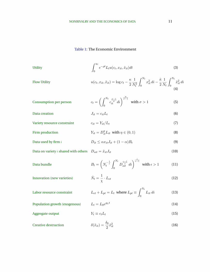
ple model above and is summarized in Table 1. There is a representative consumer with
log utility over per capita consumption, ct. There are Nt varieties of consumer goods
that combine to enter utility with a constant elasticity of substitution (CES) aggregator.
There are Lt people in the economy and population grows exogenously at rate gL.
Privacy considerations also enter flow utility in two ways, as seen in equation (4).
The first is via xit, which denotes the fraction of an individual’s data on consumption of
variety i that is used by the firm producing that variety. The second is through xit, which
denotes the fraction of an individual’s data on variety i that is used by other firms in the
1We are holding firm size ν constant in this comparative static, which meansLmust be rising asN rises.This is exactly the source of the scale effect we are considering. In the full model, this is micro-foundedthrough entry.
NONRIVALRY AND THE ECONOMICS OF DATA 11
Table 1: The Economic Environment
Utility
∫ ∞0
e−ρtLtu(ct, xit, xit)dt (3)
Flow Utility u(ct, xit, xit) = log ct −κ
2
1
N2t
∫ Nt
0x2it di−
κ
2
1
Nt
∫ Nt
0x2it di
(4)
Consumption per person ct =
(∫ Nt
0cσ−1σ
it di
) σσ−1
with σ > 1 (5)
Data creation Jit = citLt (6)
Variety resource constraint cit = Yit/Lt (7)
Firm production Yit = DηitLit with η ∈ (0, 1) (8)
Data used by firm i Dit ≤ αxitJit + (1− α)Bt (9)
Data on variety i shared with others Dsit = xitJit (10)
Data bundle Bt =
(N− 1ε
t
∫ Nt
0D
ε−1ε
sit di
) εε−1
with ε > 1 (11)
Innovation (new varieties) Nt =1
χ· Let (12)
Labor resource constraint Let + Lpt = Lt where Lpt ≡∫ Nt
0Lit di (13)
Population growth (exogenous) Lt = L0egLt (14)
Aggregate output Yt ≡ ctLt (15)
Creative destruction δ(xit) =δ0
2x2it (16)
12 JONES AND TONETTI
economy. For example, xit could denote the fraction of data generated by Tesla drivers
that is used by Tesla, while xit is the fraction of that Tesla driving data that is used by
Waymo and GM. Privacy costs enter via a quadratic loss function, where κ and κ capture
the weight on privacy versus consumption. Because there are Nt varieties, we add up
the privacy costs across all varieties and then assume the utility cost of privacy depends
on the average. There is an additional 1/Nt scaling of the xit privacy cost. Because
xit reflects costs associated with data use by all other (Nt) firms in the economy, it is
natural that there is a factor of Nt difference between these costs, and this formulation
generates interior solutions along the balanced growth path.
A simplifying assumption is that the unweighted average of xit and xit enters utility.
A more natural alternative would be to weight by the share of good i in the consumption
bundle. In the more natural case, consumers would be tempted to buy more of a variety
from a firm that better respects privacy. Our unweighted average shuts down this force,
which simplifies the algebra without changing the spirit of the model.
Where does data come from? Each unit of consumption is assumed to generate one
unit of data as a byproduct. This is our “learning by doing” formulation and is captured
in equation (6): Jit = citLt = Yit, where Jit is data created about variety i.
Firm i produces variety i according to equation (8) in the table, just as in the simple
model:
Yit = DηitLit, with η ∈ (0, 1)
where Dit is the amount of data used in producing variety i and Lit is labor. As be-
fore, the parameter η captures the importance of data. We will show some evidence in
Section 9 suggesting that η might take a value of 0.03 to 0.10; we think of it as a small
positive number.2
Data used by firm i is the sum of two terms:
Dit ≤ αxitJit + (1− α)Bt.
The first term captures the amount of variety i data that is used to help firm i produce.
In some of our allocations, firm iwill be able to use all the variety i data — for example if
firms own data. However, if consumers own data, they may restrict the amount of data
2We require η < 1/σ. For firm size to be finite, the increasing returns from data must be smaller thanthe price elasticity with respect to size coming from CES demand.
NONRIVALRY AND THE ECONOMICS OF DATA 13
that firms are able to use (xit < 1). The second part of the equation incorporates data
from other varieties that is used by firm i. Shared data on other varieties is aggregated
into a bundle,Bt. For example, xitJit is the data from Tesla drivers that Tesla gets to use
while Bt is the bundle of data from other self-driving car companies like Waymo, GM,
and Uber that is also available to Tesla. The weights α and 1−α govern the importance
of own versus others’ data. The way the aggregate bundleBt enters the individual firm’s
constraint in equation (9) is the most important feature of the model. This expression
incorporates the key role of the nonrivalry of data: the bundle Bt can be used by any
number of firms simultaneously; hence it does not have an i subscript.
How is the bundle of data created? Let Dsit ≡ xitJit denote the data about variety i
that is “shared” (hence the “s” subscript) and available for use by other firms to produce
their varieties. Shared data is bundled together via a CES production function with
elasticity of substitution ε:
Bt =
(N− 1ε
t
∫ Nt
0D
ε−1ε
sit di
) εε−1
.
We divorce the returns to variety from the elasticity of substitution in this CES function
using the method suggested by Benassy (1996). In particular, this formulation implies
that B will scale in direct proportion to N and is given by B = NDsi in the symmetric
allocation, which simplifies the analysis.
For tractability, we set up the model so that data produced today is used to produce
output today, i.e., roundabout production. We think of this as a within-period timing
assumption. We also assume that data depreciates fully every period. These two as-
sumptions imply that data is not a state variable, greatly simplifying the analysis.
The creation of new varieties is straightforward: χunits of labor are needed to create
a new variety. Total labor used for entry, Let, plus total labor used in production, Lpt,
equals total labor available in the economy, Lt.
Equation (15) in Table 1 is simply a definition. Aggregate output in the economy, Yt,
equals aggregate consumption; there is no capital.
Notice that in our environment, ideas and data are well-defined and distinct. An
idea is a blueprint for producing a distinct variety, and each new blueprint is created
by χ units of labor. Data is a byproduct of consumption, and each time a good is
14 JONES AND TONETTI
consumed, one unit of data is created that is in turn useful for improving productivity,
which can be thought of as the quality of the idea. A new idea is a new production
function for producing a variety while data is a factor of production.
Finally, equation (16) is not actually part of the economic environment, but it is
an important feature of the economy. We’ve already mentioned one downside to the
broad use of data — the privacy cost to individuals. Data sharing also increases the rate
of creative destruction: ownership of variety i changes according to a Poisson process
with an arrival rate δ(xit). The more that competitors know about an incumbent firm,
the greater the chance that the incumbent firm is displaced by an entrant. Because this
is just a change in ownership, it is not part of the technology that constrains the social
planner.
Discussion. There are alternative assumptions we could make about our economic
environment. For example, instead of having data be generated as a byproduct of
consumption, we could instead assume firms have access to a separate production
function for data (“learning or doing” instead of “learning by doing”). Both occur in
the world: Tesla gathers data while people drive their cars, while Waymo sets up its
own artificial towns in which they test-drive cars to generate data. Second, economic
growth (gL > 0) is not necessary to make most of the main points of the paper; our
results are almost entirely “level effects” rather than “growth effects” and would exist
even with no aggregate growth. The presence of growth helps bring out the distinction
between ideas and data and also simplifies the algebra. Third, we model privacy costs
as a direct utility loss. We see this as a stand in for the many reasons people may not
want firms to have their data. The main point of our paper is to highlight a way in which
the broad use of data is beneficial, not to explore the precise nature of privacy costs. We
include them to show that even when privacy costs are large, our mechanism can still
be quantitatively important.
4 The Optimal Allocation
The optimal allocation in our environment is easy to define and characterize. Using
symmetry, the production structure of the economy can be simplified considerably.
NONRIVALRY AND THE ECONOMICS OF DATA 15
Consumption per person is
ct = Nσσ−1
t cit = Nσσ−1
t
YitLt. (17)
Moreover, the production of a variety is
Yit = DηitLit = Dη
it ·LptNt
. (18)
Combining these two expressions, aggregate output in the symmetric economy is
Yt = N1
σ−1
t DηitLpt. (19)
Next, symmetry allows us to further simplify the data component:
Dit = αxitYit + (1− α)NtxitYit
= [αxit + (1− α)xitNt]Yit (20)
This expression can be substituted into the production function for variety i in (18) to
yield
Yit = [(αxit + (1− α)xitNt)ηLit]
11−η . (21)
The increasing returns associated with data shows up in the 1/(1 − η) exponent. Also,
the term αxit+(1−α)xitNt will appear frequently whenever data is shared. This deriva-
tion shows that the αxit piece reflects firms using data from their own variety while the
(1−α)xitNt piece reflects firms using data from other varieties. Moreover, when data is
shared, this data term scales with the measure of varieties,Nt. This ultimately provides
an extra scale effect associated with data nonrivalry.
Finally, substituting the expression for Dit into the aggregate production function
in (19) and using Lit = Lpt/Nt yields
Yt = N1
σ−1
t
(αxitNt
+ (1− α)xit
) η1−η
L1
1−ηpt . (22)
This equation captures the two sources of increasing returns in our model. The N1
σ−1
t
16 JONES AND TONETTI
is the standard increasing returns from love-of-variety associated with the nonrivalry
of ideas. The L1
1−ηpt captures the increasing returns associated with data. In the optimal
allocation, both play important roles.
We can now state the social planner problem concisely. The key allocations that
need to be determined are how to allocate labor between production and entry and
how much data to share. The optimal allocation solves
max{Lpt,xit,xit}
∫ ∞0
e−ρtL0u(ct, xit, xit) dt, ρ ≡ ρ− gL (23)
s.t.
ct = Yt/Lt
Yt = N1
σ−1
t
(αxitNt
+ (1− α)xit
) η1−η
L1
1−ηpt
Nt =1
χ(Lt − Lpt)
Lt = L0egLt
The planner wants to share variety i data with firm i because that increases pro-
ductivity and output. Similarly, the planner wants to share variety i data with other
firms to take advantage of the nonrivalry of data, increasing the productivity and out-
put of all firms. Tempering the planner’s desire for sharing are consumers’ privacy
concerns. Finally, the planner weighs the gains from new varieties against the gains
from producing more of the existing varieties when allocating labor to production and
entry. The optimal allocation is given in Proposition 1.
Proposition 1 (The Optimal Allocation): Along a balanced growth path, as Nt grows
large, the optimal allocation converges to
xit = xsp =
(1
κ· η
1− η
)1/2
(24)
xit = xsp =α
1− α· κκ
(1
κ· η
1− η
)1/2
(25)
Lspi = χρ · σ − 1
1− η≡ νsp (26)
NONRIVALRY AND THE ECONOMICS OF DATA 17
N spt =
LtχgL + νsp
≡ ψspLt (27)
Lsppt = νspψspLt (28)
Y spt =
[νsp(1− α)ηxηsp
] 11−η (ψspLt)
1σ−1
+ 11−η (29)
cspt =YtLt
=[νsp(1− α)ηxηsp
] 11−η ψ
1σ−1
+ 11−η
sp L1
σ−1+ η
1−ηt (30)
gspc =
(1
σ − 1+
η
1− η
)gL (31)
Dspi = [(1− α)xspνspψspLt]
11−η (32)
Dsp = NDi = [(1− α)xspνsp]1
1−η (ψspLt)1+ 1
1−η (33)
Y spi =
[νsp(1− α)ηxηsp
] 11−η (ψspLt)
η1−η (34)
U0 =1
ρL0
(log c0 −
κ
2x2sp +
gcρ
)(35)
Proof See Appendix A.
The most important result in the proposition is the solution for aggregate output
per person in equation (30). In particular, that solution shows that output per person is
proportional to the size of the economy raised to some power. The exponent, 1σ−1 + η
1−η ,
captures the degree of increasing returns to scale in the economy and is the sum of
two terms. First is the standard “love of variety” effect that is smaller when varieties
are more substitutable. The second term is new and reflects the increasing returns
associated with the nonrivalry of data. It is increasing in η, the importance of data
to the economy. A larger economy is richer because it produces more data which then
feeds back and makes all firms more productive. This equation also makes clear why
we require η < 1; if η ≥ 1, then the degree of increasing returns to scale is so large that
the economy becomes infinitely rich: more output leads to more data, which leads to
more output, and the virtuous circle explodes.
The next equation, (31), expresses the implications for growth: the growth rate of
consumption per person, in the long run, is proportional to the growth rate of popula-
tion, where the factor of proportionality is the degree of increasing returns to scale.
The remaining results in the optimal allocation break down in a simple way. First,
optimal data sharing xsp and xsp are decreasing in the privacy costs (κ and κ) and
18 JONES AND TONETTI
increasing in the importance of data in the economy (η), as shown in equations (24)
and (25).
Next, equation (27) shows that optimal variety N spt is proportional to the popula-
tion in the economy, and the factor of proportionality is defined to be the parameter
ψsp. Higher entry costs, a higher rate of time preference, and faster population growth
all reduce variety along the balanced growth path. A higher elasticity of substitution
between varieties makes new varieties less valuable and reduces N spt . Finally, if data
is more important (↑ η) the economy devotes less resources to entry (which does not
create data) and more resources to production (which does).
This is even more apparent in equation (26), which shows employment per firm,
Lspit , which equals a combination of parameters that we define to be νsp. The compa-
rative statics for firm size are essentially the opposite of those for variety. Optimal firm
size is constant along a balanced growth path and invariant to the overall population of
the economy. This reflects the assumption that the entry cost is a fixed amount of labor
that does not change as the economy grows. The fact that the size distribution of firms
seems stationary in the U.S. suggests this may be a reasonable assumption as Bollard,
Klenow and Li (2016) document. We show later that the key findings of our paper are
robust to variations of this assumption.
We will return to these results after discussing other ways to allocate resources in
this environment. The ν and ψ parameters for the different allocations will be an im-
portant part of that comparison.
5 Firms Own Data
We now explore one possible way to use markets to allocate resources. In this equi-
librium, we assume that firms own data and decide whether or not to sell it. Data is
bought and sold via a data intermediary that bundles together data from all varieties
and resells it to each individual firm. Throughout the paper, buyers of data are always
price takers and sellers of data always set prices.
NONRIVALRY AND THE ECONOMICS OF DATA 19
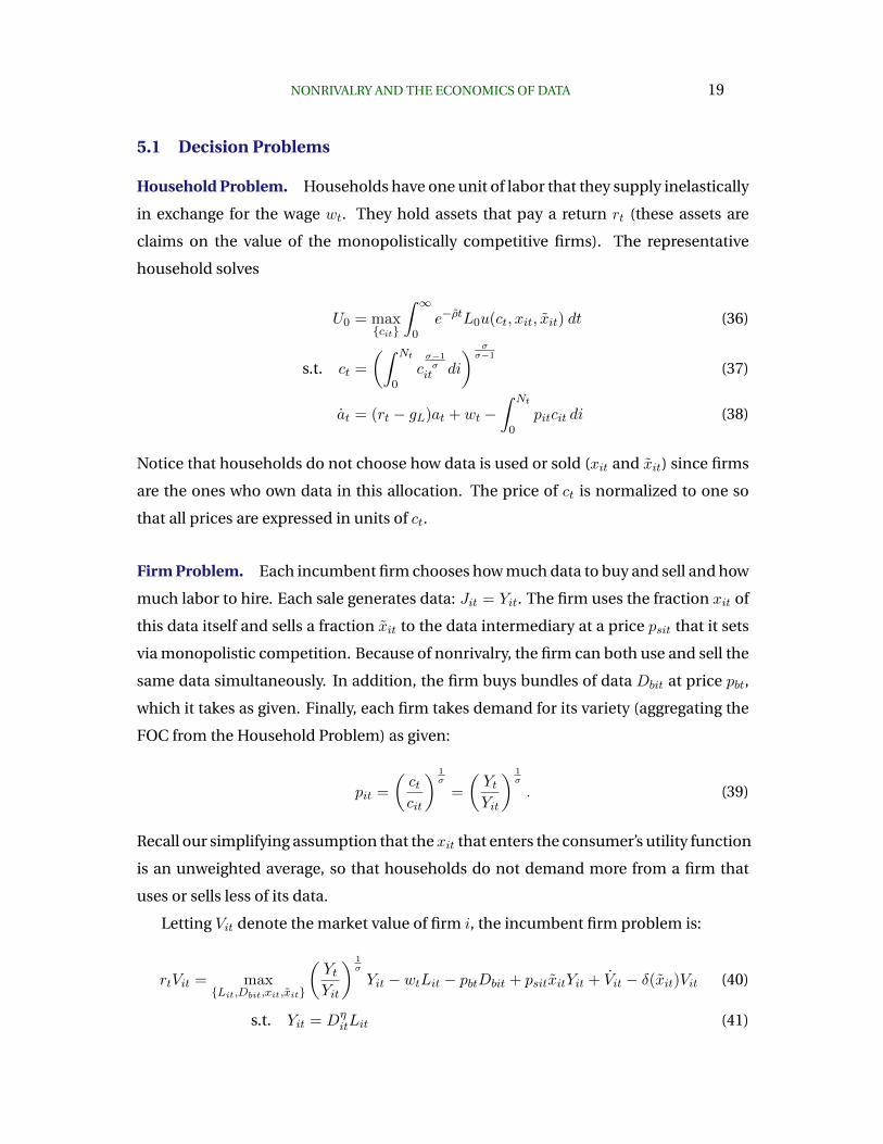
5.1 Decision Problems
Household Problem. Households have one unit of labor that they supply inelastically
in exchange for the wage wt. They hold assets that pay a return rt (these assets are
claims on the value of the monopolistically competitive firms). The representative
household solves
U0 = max{cit}
∫ ∞0
e−ρtL0u(ct, xit, xit) dt (36)
s.t. ct =
(∫ Nt
0cσ−1σ
it di
) σσ−1
(37)
at = (rt − gL)at + wt −∫ Nt
0pitcit di (38)
Notice that households do not choose how data is used or sold (xit and xit) since firms
are the ones who own data in this allocation. The price of ct is normalized to one so
that all prices are expressed in units of ct.
Firm Problem. Each incumbent firm chooses how much data to buy and sell and how
much labor to hire. Each sale generates data: Jit = Yit. The firm uses the fraction xit of
this data itself and sells a fraction xit to the data intermediary at a price psit that it sets
via monopolistic competition. Because of nonrivalry, the firm can both use and sell the
same data simultaneously. In addition, the firm buys bundles of data Dbit at price pbt,
which it takes as given. Finally, each firm takes demand for its variety (aggregating the
FOC from the Household Problem) as given:
pit =
(ctcit
) 1σ
=
(YtYit
) 1σ
. (39)
Recall our simplifying assumption that thexit that enters the consumer’s utility function
is an unweighted average, so that households do not demand more from a firm that
uses or sells less of its data.
Letting Vit denote the market value of firm i, the incumbent firm problem is:
rtVit = max{Lit,Dbit,xit,xit}
(YtYit
) 1σ
Yit − wtLit − pbtDbit + psitxitYit + Vit − δ(xit)Vit (40)
s.t. Yit = DηitLit (41)
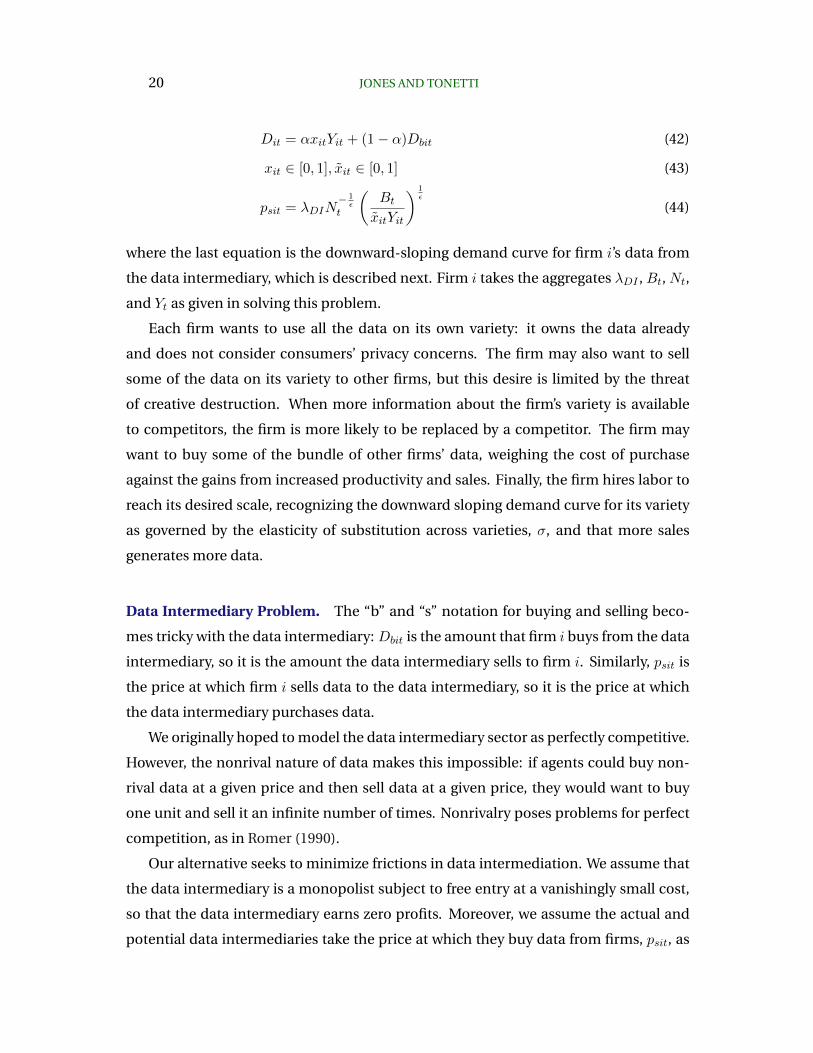
20 JONES AND TONETTI
Dit = αxitYit + (1− α)Dbit (42)
xit ∈ [0, 1], xit ∈ [0, 1] (43)
psit = λDIN− 1ε
t
(BtxitYit
) 1ε
(44)
where the last equation is the downward-sloping demand curve for firm i’s data from
the data intermediary, which is described next. Firm i takes the aggregates λDI , Bt, Nt,
and Yt as given in solving this problem.
Each firm wants to use all the data on its own variety: it owns the data already
and does not consider consumers’ privacy concerns. The firm may also want to sell
some of the data on its variety to other firms, but this desire is limited by the threat
of creative destruction. When more information about the firm’s variety is available
to competitors, the firm is more likely to be replaced by a competitor. The firm may
want to buy some of the bundle of other firms’ data, weighing the cost of purchase
against the gains from increased productivity and sales. Finally, the firm hires labor to
reach its desired scale, recognizing the downward sloping demand curve for its variety
as governed by the elasticity of substitution across varieties, σ, and that more sales
generates more data.
Data Intermediary Problem. The “b” and “s” notation for buying and selling beco-
mes tricky with the data intermediary: Dbit is the amount that firm i buys from the data
intermediary, so it is the amount the data intermediary sells to firm i. Similarly, psit is
the price at which firm i sells data to the data intermediary, so it is the price at which
the data intermediary purchases data.
We originally hoped to model the data intermediary sector as perfectly competitive.
However, the nonrival nature of data makes this impossible: if agents could buy non-
rival data at a given price and then sell data at a given price, they would want to buy
one unit and sell it an infinite number of times. Nonrivalry poses problems for perfect
competition, as in Romer (1990).
Our alternative seeks to minimize frictions in data intermediation. We assume that
the data intermediary is a monopolist subject to free entry at a vanishingly small cost,
so that the data intermediary earns zero profits. Moreover, we assume the actual and
potential data intermediaries take the price at which they buy data from firms, psit, as
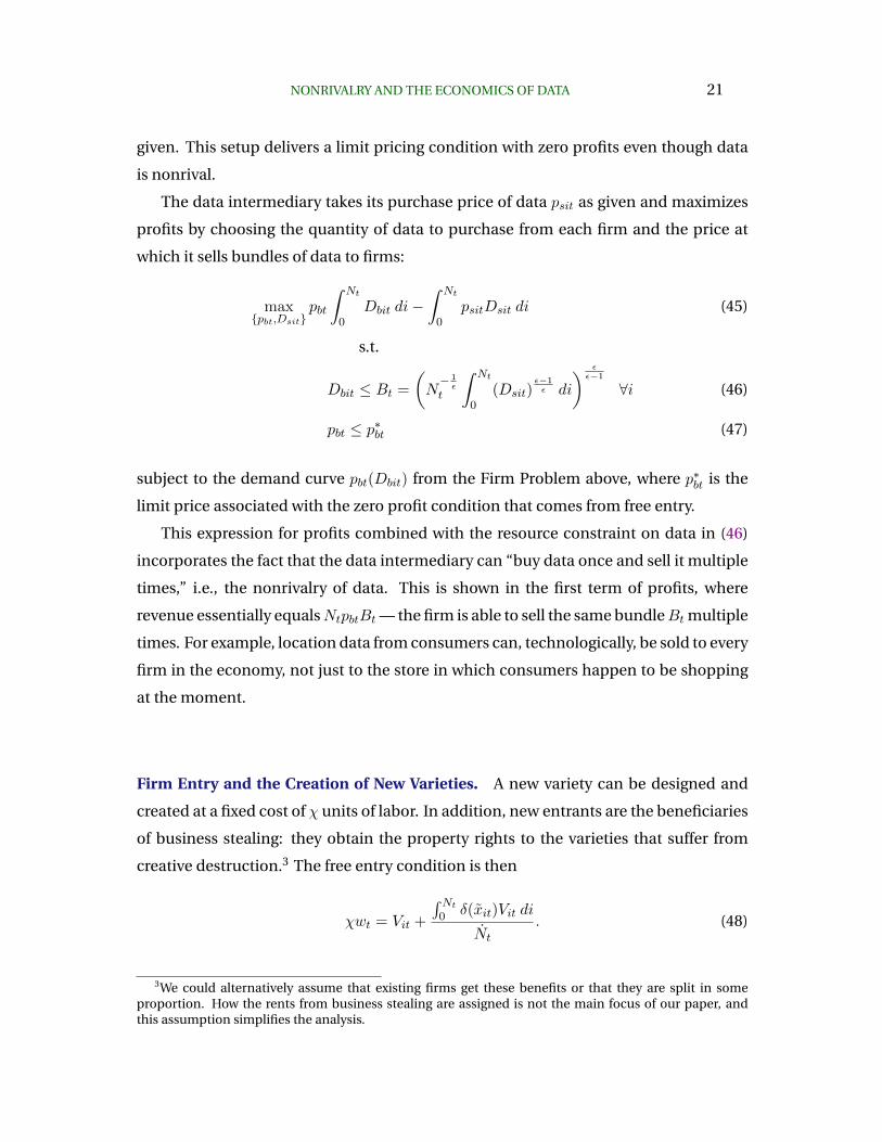
NONRIVALRY AND THE ECONOMICS OF DATA 21
given. This setup delivers a limit pricing condition with zero profits even though data
is nonrival.
The data intermediary takes its purchase price of data psit as given and maximizes
profits by choosing the quantity of data to purchase from each firm and the price at
which it sells bundles of data to firms:
max{pbt,Dsit}
pbt
∫ Nt
0Dbit di−
∫ Nt
0psitDsit di (45)
s.t.
Dbit ≤ Bt =
(N− 1ε
t
∫ Nt
0(Dsit)
ε−1ε di
) εε−1
∀i (46)
pbt ≤ p∗bt (47)
subject to the demand curve pbt(Dbit) from the Firm Problem above, where p∗bt is the
limit price associated with the zero profit condition that comes from free entry.
This expression for profits combined with the resource constraint on data in (46)
incorporates the fact that the data intermediary can “buy data once and sell it multiple
times,” i.e., the nonrivalry of data. This is shown in the first term of profits, where
revenue essentially equalsNtpbtBt — the firm is able to sell the same bundleBt multiple
times. For example, location data from consumers can, technologically, be sold to every
firm in the economy, not just to the store in which consumers happen to be shopping
at the moment.
Firm Entry and the Creation of New Varieties. A new variety can be designed and
created at a fixed cost of χ units of labor. In addition, new entrants are the beneficiaries
of business stealing: they obtain the property rights to the varieties that suffer from
creative destruction.3 The free entry condition is then
χwt = Vit +
∫ Nt0 δ(xit)Vit di
Nt
. (48)
3We could alternatively assume that existing firms get these benefits or that they are split in someproportion. How the rents from business stealing are assigned is not the main focus of our paper, andthis assumption simplifies the analysis.

22 JONES AND TONETTI
The left side χwt is the cost of the χ units of labor needed to create a new variety. The
right side has two terms. The first is the value of the new variety that is created. The
second, is the per-entrant portion of the rents from creative destruction.
5.2 The Equilibrium when Firms Own Data
The equilibrium in which firms own data consists of quantities {ct, Yt, cit, xit, xit, at,
Yit, Lit, Dit, Dbit, Bt, Dsit, Nt, Lpt, Let, Lt} and prices {pit, pbt, psit, wt, rt, Vit} such that
1. {ct, cit, at} solve the Household Problem
2. {Lit, Yit, pit, psit, Dbit, Dit, xit, xit, Vit} solve the Firm Problem
3. (Dsit, Bt) Data markets clear: Dbit = Bt and Dsit = xitYit
4. (pbt) Free entry into data intermediation gives zero profits there (constrains pb as
a function of ps)
5. (Let) Free entry into producing a new variety leads to zero profits, as in equa-
tion (48)
6. Definition of Lpt: Lpt =∫ Nt
0 Lit di
7. wt clears the labor market: Lpt + Let = Lt
8. rt clears the asset market: atLt =∫ Nt
0 Vit di
9. Nt follows its law of motion: Nt = 1χ(Lt − Lpt)
10. Yt ≡ ctLt denotes aggregate output
11. Exogenous population growth: Lt = L0egLt
In Section 8, we compare the allocation that results from this equilibrium with the
optimal allocation as well as with alternative allocations. Before that, we define the
alternative allocations, allowing us to efficiently make the comparisons all at once. For
this reason, we turn next to an equilibrium in which consumers own data.
NONRIVALRY AND THE ECONOMICS OF DATA 23
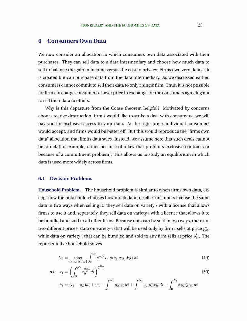
6 Consumers Own Data
We now consider an allocation in which consumers own data associated with their
purchases. They can sell data to a data intermediary and choose how much data to
sell to balance the gain in income versus the cost to privacy. Firms own zero data as it
is created but can purchase data from the data intermediary. As we discussed earlier,
consumers cannot commit to sell their data to only a single firm. Thus, it is not possible
for firm i to charge consumers a lower price in exchange for the consumers agreeing not
to sell their data to others.
Why is this departure from the Coase theorem helpful? Motivated by concerns
about creative destruction, firm i would like to strike a deal with consumers: we will
pay you for exclusive access to your data. At the right price, individual consumers
would accept, and firms would be better off. But this would reproduce the “firms own
data” allocation that limits data sales. Instead, we assume here that such deals cannot
be struck (for example, either because of a law that prohibits exclusive contracts or
because of a commitment problem). This allows us to study an equilibrium in which
data is used more widely across firms.
6.1 Decision Problems
Household Problem. The household problem is similar to when firms own data, ex-
cept now the household chooses how much data to sell. Consumers license the same
data in two ways when selling it: they sell data on variety i with a license that allows
firm i to use it and, separately, they sell data on variety i with a license that allows it to
be bundled and sold to all other firms. Because data can be sold in two ways, there are
two different prices: data on variety i that will be used only by firm i sells at price past,
while data on variety i that can be bundled and sold to any firm sells at price pbst. The
representative household solves
U0 = max{cit,xit,xit}
∫ ∞0
e−ρtL0u(ct, xit, xit) dt (49)
s.t. ct =
(∫ Nt
0cσ−1σ
it di
) σσ−1
(50)
at = (rt − gL)at + wt −∫ Nt
0pitcit di+
∫ Nt
0xitp
astcit di+
∫ Nt
0xitp
bstcit di
24 JONES AND TONETTI
= (rt − gL)at + wt −∫ Nt
0qitcit dt (51)
where qit ≡ pit − xitpast − xitp
bst is the effective price of consumption, taking into ac-
count that the fractions xit and xit of each good consumed generate income when the
associated data is sold.
Firm Problem. Each incumbent firm chooses how much data to buy. Two types of
data are available for purchase: data from the firm’s own variety (Dait) and data from
other varieties (Dbit). Each firm sees the downward-sloping demand for its variety
(aggregating the FOC from the Household Problem):
qit =
(ctcit
) 1σ
=
(YtYit
) 1σ
= pit − xitpast − xitpbst (52)
so that
pit =
(YtYit
) 1σ
+ xitpast + xitp
bst. (53)
Letting Vit denote the market value of firm i, the incumbent firm problem is:
rtVit = maxLit,Dait,Dbit
[(YtYit
) 1σ
+ xitpast + xitp
bst
]Yit − wtLit − patDait − pbtDbit
+ Vit − δ(xit)Vit (54)
s.t. Yit = DηitLit
Dit = αDait + (1− α)Dbit (55)
Dait ≥ 0, Dbit ≥ 0
Firms no longer face a simple constant elasticity demand curve because the ef-
fective price that consumers pay is different from the price that firms receive (because
consumers sell data). From the perspective of the firm,Dait andDbit are perfect substi-
tutes: the firm is indifferent between using its own data versus an appropriately-sized
bundle of other firms’ data. This fact will help pin down the relative price of the two
kinds of data.

NONRIVALRY AND THE ECONOMICS OF DATA 25
Data Intermediary Problem. Because we have two types of data, we now introduce
two different data intermediaries: one handles the sale of “own” data and the other
handles the bundle. Each is modeled as earlier, i.e., as a monopolist who is constrained
by free entry into data intermediation.
Taking the price past of data purchased from consumers as given, the data interme-
diary for own data solves the following problem at each date t:
max{pait,Dacit}
∫ Nt
0paitDait di−
∫ Nt
0pastD
acit di (56)
s.t.
Dait ≤ Dacit ∀i (57)
pait ≤ p∗ait (58)
subject to the demand curve pait(Dait) from the Firm Problem above, where p∗ait is the
limit price associated with the zero profit condition that comes from free entry.
Similarly, taking the price pbst of data purchased from consumers as given, the data
intermediary for bundled data solves
max{pbit,Dbcit}
∫ Nt
0pbitDbit di−
∫ Nt
0pbstD
bcit di (59)
s.t.
Dbit ≤ Bt =
(N− 1ε
t
∫ Nt
0(Db
cit)ε−1ε di
) εε−1
∀i (60)
pbit ≤ p∗bit (61)
subject to the demand curve pbit (Dbit) from the Firm Problem above, where p∗bit is the
limit price associated with the zero profit condition that comes from free entry.
The two data intermediaries are monopolists who choose the prices pait and pbit
of data as well as how much data to buy from consumers of each variety and type,
taking the prices past and pbst as given. From the standpoint of the consumer, one unit
of consumption generates one unit of data and data from all varieties sell at the same
price, while each type of license may sell at a different price.
The constraints on the data intermediary problems are critical. Equation (57) says
that the largest amount of own data the intermediary can sell to firm i is the amount
26 JONES AND TONETTI
of variety i data that the data intermediary has purchased. In contrast, equation (60)
recognizes that data from all varieties can be bundled together and resold to each indi-
vidual firm.
We assume free entry into the data intermediary sector at zero cost. This constrains
the prices pa and pb that the data intermediaries can charge and implies that the mo-
nopolist earns zero profits. This condition together with the fact that the two types of
data are perfect substitutes in the firm production function pin down the prices.
6.2 Equilibrium when Consumers Own Data
An equilibrium in which consumers own data consists of quantities {ct, Yt, cit, xit, xit, at,
Yit, Lit, Dit, Dait, Dbit, Dacit, D
bcit, Bt, Nt, Lpt, Let, Lt} and prices {qit, pit, pait, pbit, past, pbst, wt,
rt, Vit} such that
1. {ct, cit, xit, xit, at} solve the Household Problem
2. {Lit, Yit, pit, Dait, Dbit, Dit, Vit} solve the Firm Problem
3. (qit) The effective consumer price is qit = pit − xitpast − xitpbst
4. Dacit, D
bcit, Bt, pait, and pbit solve the Data Intermediary Problem subject to the
constraint that there is free entry into this sector, so it makes zero profits
5. past clears the data market so that supply equals demand: Dacit = xitcitLt
6. pbst clears the data market so that supply equals demand: Dbcit = xitcitLt
7. (Let) Free entry into producing a new variety leads to zero profits (including the
entrant’s share of the rents from creative destruction): χwt = Vit +∫Nt0 δ(xit)Vit di
Nt
8. Definition of Lpt: Lpt =∫ Nt
0 Lit di
9. wt clears the labor market: Lpt + Let = Lt
10. rt clears the asset market: atLt =∫ Nt
0 Vit di
11. Nt follows its law of motion: Nt = 1χ(Lt − Lpt)
12. Yt ≡ ctLt denotes aggregate output
13. Exogenous population growth: Lt = L0egLt
NONRIVALRY AND THE ECONOMICS OF DATA 27
6.3 Understanding the Equilibrium when Consumers Own Data
While Section 8 will discuss the key features of this allocation, it is worth pausing here
to highlight some smaller results.
First, because own data and the bundle of other-variety data are perfect substitutes
(see equation (55)), in equilibrium
pat =α
1− αpbt (62)
where we’ve dropped the i subscript because of symmetry. At any other price ratio,
firms would buy only one type of data and not the other. Similarly, the consumer prices
for each type of data satisfy
past = pat and pbst = Ntpbt. (63)
Second, consider the inequality constraints in the Data Intermediary problems. In
equilibrium, the data intermediary will sell any data that it buys. Moreover, because
of nonrivalry, data can be bought once and sold multiple times. This means that both
inequality constraints will bind. First, Dait = Dacit = xitYit; that is, all data on variety
i that the data intermediary purchases will be sold to firm i. Second, Dbit = Bt =
NDbcit = NxitYit (using symmetry); that is, all data that is licensed for sharing that the
data intermediary buys will be sold to all firms as bundled data.
7 Outlaw Data Sales
The final allocation that we consider is motivated by recent concerns over data privacy.
In the world in which firms own data, suppose the government, in an effort to protect
privacy, limits the use of data. In particular, it mandates that
xit = 0
xit ≤ x ∈ (0, 1].
That is, firms are not allowed to sell their data to any third parties: xit = 0. A similar
allocation without the broad use of data may arise from an opt-out law that grants con-

28 JONES AND TONETTI
sumers the right to prevent firms from selling their data, since there are privacy costs
to the consumer and no counteracting direct income gain. Moreover, the government
may restrict firms to use less than 100 percent of their own-variety data, parameterized
by xit = x. We require x > 0 in our setting — otherwise output of each firm would be
zero because data is an essential input to production.
With this determination of xit and xit, the rest of the equilibrium looks exactly like
the firms-own-data case, so we will not repeat that setup here. Instead, we turn next to
comparing the equilibrium outcomes across these different allocations.
8 Key Insights from Comparing the Different Allocations
This section delivers the payoff from the preparation we’ve made in the previous secti-
ons: we see how the different allocation mechanisms we’ve studied lead to different
outcomes. We compare the allocations on the balanced growth path for the social
planner (sp), when consumers own data (c), when firms own data (f ), and when the
government outlaws the selling of data (os). When firms restrict the sale of data to limit
their exposure to creative destruction, what are the consequences? When consumers
own data and can sell it, is the allocation optimal? What if selling data is banned out of
a concern for privacy?
Privacy and Data Sales. The steady-state fraction of data that is used by other firms
is given by4
xsp =
(1
κ· η
1− η
)1/2
(64)
xc =
(1
κ· η
1− η· σ − 1
σ
)1/2
(65)
xf =
(2Γρ
(2− Γ)δ0
)1/2
where Γ ≡ η(σ − 1)εε−1 − ση
(66)
xos = 0. (67)
Interestingly, even when consumers own and sell their data, the equilibrium allocation
features inefficiently low data sales because of the σ−1σ < 1 term in equation (65). The
4We assume εε−1
> ση and εε−1
> 32ση − 1
2η so that Γ ∈ (0, 2) holds in equation (66).
NONRIVALRY AND THE ECONOMICS OF DATA 29
equilibrium price of data that consumers receive in exchange for selling is influenced
by this same factor:
pbst =η
1− η· σ − 1
σ· 1
xc(ψcLt)
1σ−1 .
Recall that σσ−1 is the standard monopoly markup in the goods market, so the intuition
is that the monopoly markup distortion leads data to sell for a price that is inefficiently
low, causing consumers to sell too little data.
The strong similarity between the consumer and optimal x can be contrasted with
data sales when firms own data, given in equation (66). First, the utility cost associated
with privacy κ does not enter the firm solution, as firms do not inherently care about
privacy. Second, xf depends on δ0, capturing the crucial role of creative destruction
— which does not enter the planner or consumer solutions for x. As we will see in our
numerical examples, reasonable values for δ0 mean that creative destruction concerns
are first-order for firms, so they may sell little data to other firms and choose a small xf .
Thus, firms inadvertently deliver privacy benefits to consumers. But as we will see, this
aversion to selling data has other consequences. An extreme version of this allocation
is the one that outlaws data sales entirely, so that xos = 0.
The privacy considerations that involve only firm i and consumption of variety i are
similar. In particular,
xsp =α
1− ακ
κ· xsp (68)
xc =α
1− ακ
κ· xc (69)
xf = 1 (70)
xos = x ∈ (0, 1]. (71)
These equations show that when firms own data, they overuse it. That is, firms set
xf = 1, while the social planner and consumers take into account the privacy costs
associated with κ and generally choose less direct use of data, xc < xsp < 1.
Firm Size. Because of symmetry, firm size Lit equals the ratio of production employ-
ment to varieties, Lpt/Nt. This quantity plays an important role in all of the allocations
30 JONES AND TONETTI
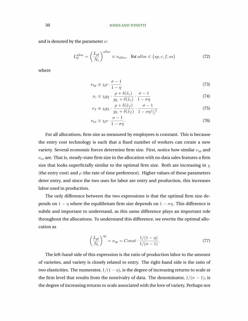
and is denoted by the parameter ν:
Lallocit =
(LptNt
)alloc≡ νalloc, for alloc ∈ {sp, c, f, os} (72)
where
νsp ≡ χρ ·σ − 1
1− η(73)
νc ≡ χgL ·ρ+ δ(xc)
gL + δ(xc)· σ − 1
1− ση(74)
νf ≡ χgL ·ρ+ δ(xf )
gL + δ(xf )· σ − 1
1− ση ε−1ε
(75)
νos ≡ χρ ·σ − 1
1− ση. (76)
For all allocations, firm size as measured by employees is constant. This is because
the entry cost technology is such that a fixed number of workers can create a new
variety. Several economic forces determine firm size. First, notice how similar νsp and
νos are. That is, steady-state firm size in the allocation with no data sales features a firm
size that looks superficially similar to the optimal firm size. Both are increasing in χ
(the entry cost) and ρ (the rate of time preference). Higher values of these parameters
deter entry, and since the two uses for labor are entry and production, this increases
labor used in production.
The only difference between the two expressions is that the optimal firm size de-
pends on 1 − η where the equilibrium firm size depends on 1 − ση. This difference is
subtle and important to understand, as this same difference plays an important role
throughout the allocations. To understand this difference, we rewrite the optimal allo-
cation as (LptNt
)sp= νsp = Const · 1/(1− η)
1/(σ − 1). (77)
The left-hand side of this expression is the ratio of production labor to the amount
of varieties, and variety is closely related to entry. The right-hand side is the ratio of
two elasticities. The numerator, 1/(1− η), is the degree of increasing returns to scale at
the firm level that results from the nonrivalry of data. The denominator, 1/(σ − 1), is
the degree of increasing returns to scale associated with the love of variety. Perhaps not

NONRIVALRY AND THE ECONOMICS OF DATA 31
surprisingly, the planner makes the ratio of production labor to the amount of varieties
proportional to the ratio of these two elasticities, which capture the social value of
production labor and entry.
In contrast, consider the equilibrium allocation when selling data is outlawed. Flip-
ping the numerator and denominator, equation (76) can be expressed as(Nt
Lpt
)os=
1
νos= Const · 1− ση
σ − 1. (78)
As shown in Appendix equation (A.67), this expression derives from the free entry con-
dition for firms, i.e., χwt = Vit (since there is no creative destruction in the outlaw-
sales equilibrium). The value of a firm is the present discounted value of future profits.
The number of firms in the economy, Nt, depends on profits relative to entry costs.
Aggregate profits as a share of aggregate output equals (1 − ση)/σ · 1/(1 − η), while
aggregate payments to production labor as a share of output equals (σ−1)/σ ·1/(1−η).
Equation (78) says that equilibrium variety is proportional to this ratio. And the inverse
of this expression gives νos.
Equations (73) and (76) imply that firm employment is larger in the equilibrium
with no data sales than in the optimal allocation since σ > 1. This occurs because
of the profit share term. Intuitively, the equilibrium allocation creates varieties based
on profits, while the social planner creates varieties based on the full social surplus.
Because profits are less than social surplus — the standard appropriability problem
— the outlaw-sales equilibrium features too few firms. The flip side is that firms in
equilibrium are inefficiently large.
We will discuss the equations for νc and νf after considering the number of firms
and varieties, next.
Number of Firms and Varieties. The effect of the appropriability problem on the
measure of varieties can be seen more directly in our next set of equations. The number
of firms (varieties) in an allocation is proportional to the labor force:
Nalloct = ψallocLt where ψalloc ≡
1
χgL + νalloc. (79)

32 JONES AND TONETTI
Notice that the last half of the denominator of the ψ expression is just the ν term itself.
For gL small, variety is basically inversely proportional to firm size, verifying intuition
provided above about firm size and variety.
Next, we compare firm size and variety between the equilibrium in which consu-
mers own data and the outlaw-sales equilibrium in which firms own data. Equati-
ons (74) and (76) show that firm sizes differ in these two allocations only because of
creative destruction, which enters in two ways. In the numerator of (74), there is a
ρ+δ(xc) term. This captures the extent to which creative destruction raises the effective
rate at which firms discount future profits. In the denominator, however, there is an
additional term involving δ(xc). This term captures the rents from destroyed firms as
they flow to new entrants — business stealing — essentially raising the return to entry.
If ρ = gL, then these two terms cancel and creative destruction does not influence firm
size and variety creation.
A similar effect impacts firm size and the number of firms in the equilibrium when
firms own data and can legally buy and sell it, as seen in equation (75). However, in that
allocation, data sales are typically lower than when consumers own data, implying that
creative destruction is also lower, reducing the role of this term.
Aggregate Output and Economic Growth. The key finding of the paper is how data
use influences living standards. The next set of equations shows aggregate output in
the various allocations. For the allocations that feature some data sharing, the equation
for aggregate output is
Y alloct =
[νalloc(1− α)ηxηalloc
] 11−η (ψallocLt)
1+ 1σ−1
+ η1−η for alloc ∈ {sp, c, f}. (80)
There are essentially three key terms in this expression, and all have a clear interpre-
tation. First, νalloc captures the size of each individual firm, and it is raised to the
power 1/(1 − η) because of the increasing returns to scale at the firm level associated
with data. Second, the term (1 − α)xalloc captures data. In particular, recall (e.g., from
equation (33)) that
Dit = [αxit + (1− α)xitNt]Yit = Nt
[αxitNt
+ (1− α)xit
]Yit. (81)
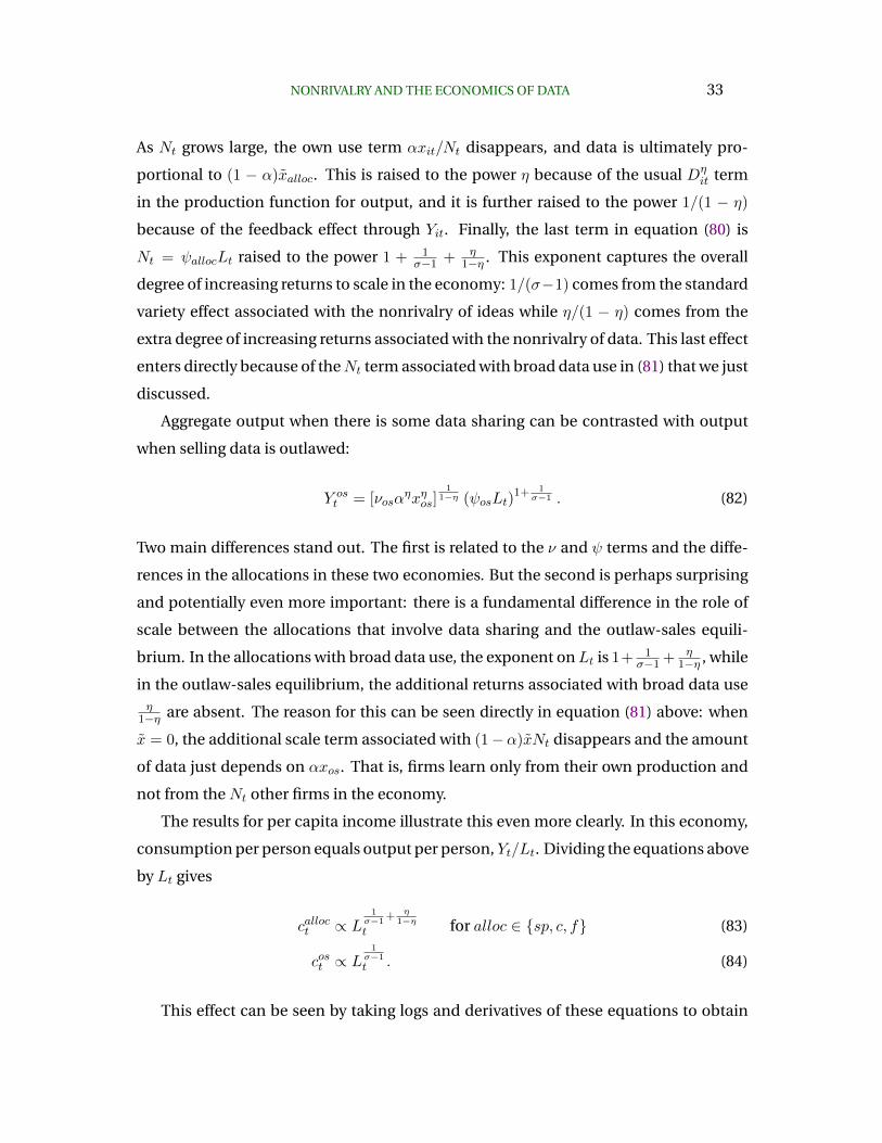
NONRIVALRY AND THE ECONOMICS OF DATA 33
As Nt grows large, the own use term αxit/Nt disappears, and data is ultimately pro-
portional to (1 − α)xalloc. This is raised to the power η because of the usual Dηit term
in the production function for output, and it is further raised to the power 1/(1 − η)
because of the feedback effect through Yit. Finally, the last term in equation (80) is
Nt = ψallocLt raised to the power 1 + 1σ−1 + η
1−η . This exponent captures the overall
degree of increasing returns to scale in the economy: 1/(σ−1) comes from the standard
variety effect associated with the nonrivalry of ideas while η/(1 − η) comes from the
extra degree of increasing returns associated with the nonrivalry of data. This last effect
enters directly because of theNt term associated with broad data use in (81) that we just
discussed.
Aggregate output when there is some data sharing can be contrasted with output
when selling data is outlawed:
Y ost = [νosα
ηxηos]1
1−η (ψosLt)1+ 1
σ−1 . (82)
Two main differences stand out. The first is related to the ν and ψ terms and the diffe-
rences in the allocations in these two economies. But the second is perhaps surprising
and potentially even more important: there is a fundamental difference in the role of
scale between the allocations that involve data sharing and the outlaw-sales equili-
brium. In the allocations with broad data use, the exponent onLt is 1+ 1σ−1 + η
1−η , while
in the outlaw-sales equilibrium, the additional returns associated with broad data useη
1−η are absent. The reason for this can be seen directly in equation (81) above: when
x = 0, the additional scale term associated with (1−α)xNt disappears and the amount
of data just depends on αxos. That is, firms learn only from their own production and
not from the Nt other firms in the economy.
The results for per capita income illustrate this even more clearly. In this economy,
consumption per person equals output per person, Yt/Lt. Dividing the equations above
by Lt gives
calloct ∝ L1
σ−1+ η
1−ηt for alloc ∈ {sp, c, f} (83)
cost ∝ L1
σ−1
t . (84)
This effect can be seen by taking logs and derivatives of these equations to obtain
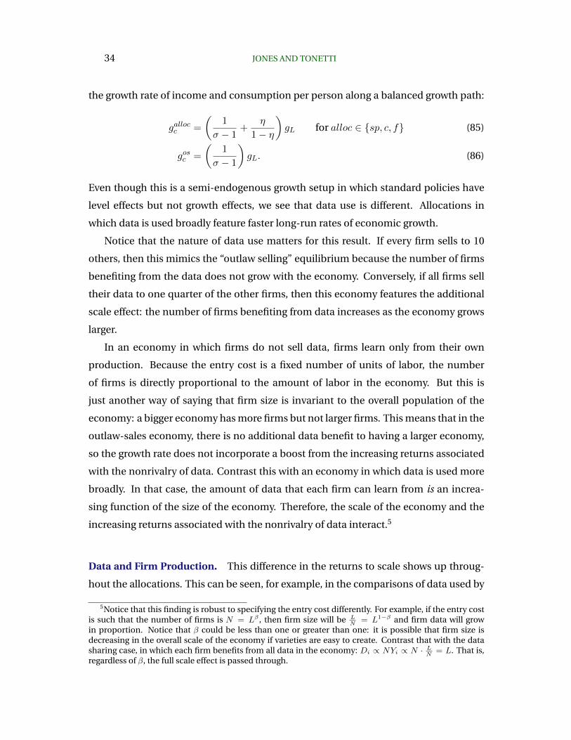
34 JONES AND TONETTI
the growth rate of income and consumption per person along a balanced growth path:
gallocc =
(1
σ − 1+
η
1− η
)gL for alloc ∈ {sp, c, f} (85)
gosc =
(1
σ − 1
)gL. (86)
Even though this is a semi-endogenous growth setup in which standard policies have
level effects but not growth effects, we see that data use is different. Allocations in
which data is used broadly feature faster long-run rates of economic growth.
Notice that the nature of data use matters for this result. If every firm sells to 10
others, then this mimics the “outlaw selling” equilibrium because the number of firms
benefiting from the data does not grow with the economy. Conversely, if all firms sell
their data to one quarter of the other firms, then this economy features the additional
scale effect: the number of firms benefiting from data increases as the economy grows
larger.
In an economy in which firms do not sell data, firms learn only from their own
production. Because the entry cost is a fixed number of units of labor, the number
of firms is directly proportional to the amount of labor in the economy. But this is
just another way of saying that firm size is invariant to the overall population of the
economy: a bigger economy has more firms but not larger firms. This means that in the
outlaw-sales economy, there is no additional data benefit to having a larger economy,
so the growth rate does not incorporate a boost from the increasing returns associated
with the nonrivalry of data. Contrast this with an economy in which data is used more
broadly. In that case, the amount of data that each firm can learn from is an increa-
sing function of the size of the economy. Therefore, the scale of the economy and the
increasing returns associated with the nonrivalry of data interact.5
Data and Firm Production. This difference in the returns to scale shows up throug-
hout the allocations. This can be seen, for example, in the comparisons of data used by
5Notice that this finding is robust to specifying the entry cost differently. For example, if the entry costis such that the number of firms is N = Lβ , then firm size will be L
N= L1−β and firm data will grow
in proportion. Notice that β could be less than one or greater than one: it is possible that firm size isdecreasing in the overall scale of the economy if varieties are easy to create. Contrast that with the datasharing case, in which each firm benefits from all data in the economy: Di ∝ NYi ∝ N · L
N= L. That is,
regardless of β, the full scale effect is passed through.
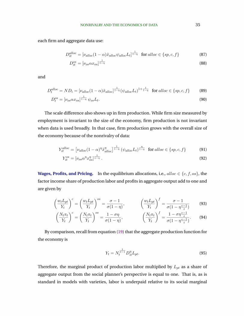
NONRIVALRY AND THE ECONOMICS OF DATA 35
each firm and aggregate data use:
Dallocit = [νalloc(1− α)xallocψallocLt]
11−η for alloc ∈ {sp, c, f} (87)
Dosit = [νosαxos]
11−η (88)
and
Dalloct = NDi = [νalloc(1− α)xalloc]
11−η (ψallocLt)
1+ 11−η for alloc ∈ {sp, c, f} (89)
Dost = [νosαxos]
11−η ψosLt. (90)
The scale difference also shows up in firm production. While firm size measured by
employment is invariant to the size of the economy, firm production is not invariant
when data is used broadly. In that case, firm production grows with the overall size of
the economy because of the nonrivalry of data:
Y allocit =
[νalloc(1− α)ηxηalloc
] 11−η (ψallocLt)
η1−η for alloc ∈ {sp, c, f} (91)
Y osit = [νosα
ηxηos]1
1−η . (92)
Wages, Profits, and Pricing. In the equilibrium allocations, i.e., alloc ∈ {c, f, os}, the
factor income share of production labor and profits in aggregate output add to one and
are given by
(wtLptYt
)c=
(wtLptYt
)os=
σ − 1
σ(1− η),
(wtLptYt
)f=
σ − 1
σ(1− η ε−1ε )
(93)(NtπtYt
)c=
(NtπtYt
)os=
1− σησ(1− η)
,
(NtπtYt
)f=
1− ση ε−1ε
σ(1− η ε−1ε )
. (94)
By comparison, recall from equation (19) that the aggregate production function for
the economy is
Yt = N1
σ−1
t DηitLpt. (95)
Therefore, the marginal product of production labor multiplied by Lpt as a share of
aggregate output from the social planner’s perspective is equal to one. That is, as is
standard in models with varieties, labor is underpaid relative to its social marginal
36 JONES AND TONETTI
product so that the economy can provide some profits to incentivize the creation of
new varieties.
It is also interesting to compare the monopoly markup and pricing in the different
equilibrium allocations. The price of a variety is
qcit = N1
σ−1
t = (ψcLt)1
σ−1 (96)
pcit =
(1 + η · σ − 1
σ(1− η)
)N
1σ−1
t =
(1 + η · σ − 1
σ(1− η)
)(ψcLt)
1σ−1 (97)
pfit = N1
σ−1
t = (ψfLt)1
σ−1 (98)
posit = N1
σ−1
t = (ψosLt)1
σ−1 . (99)
Two points are worth noting. First, the effective price paid by consumers (i.e., incor-
porating the fact that they can sell their data) in the consumers-own-data allocation —
qcit — and the actual price paid by consumers in the other allocations — pfit, posit — are
both equal to N1
σ−1
t . Of course, Nt will differ across these allocations, but the point is
that the consumer prices are both the same function of the number of firms. Moreover,
there is no “markup” term that shows up in this expression. This is a feature of the
exogenous labor supply in our environment. One way or the other, labor can only be
used to produce goods and so the monopoly markup does not result in a misallocation
of labor. This is true even though firms internalize that they have increasing returns
because of the learning-by-doing associated with data.
Second, notice that the price that firms receive for their sales in the consumers-
own-data equilibrium, pcit, does involve a markup term given by 1 + η · σ−1σ(1−η) . If η = 0,
this term would drop out. Instead, it captures the fact that firms know that consumers
can sell their data. Therefore, firms charge an additional markup over marginal cost to
capture this revenue.
The Value of Data. The value of data as a share of GDP is given by(Nt(patDat + pbtDbt)
Yt
)c=
η
1− ησ − 1
σ(100)(
Nt(patYit + pbtDbt)
Yt
)f=
η
1− η ε−1ε
· σ − 1
σ. (101)
NONRIVALRY AND THE ECONOMICS OF DATA 37
We will use these expressions in the numerical examples shortly.6
9 Numerical Examples
We now provide a set of numerical examples to illustrate the forces in the model. This
should not be viewed as a formal calibration that can be compared quantitatively to
facts about the U.S. economy. For example, our model assumes that all firms benefit
from data equally and that each firm’s data is equally useful. In this sense, the model
might more naturally be compared to a particular industry, such as radiology or auto-
nomous cars. Nevertheless, we find it useful to think about how large the various forces
in the model might possibly be.
How Large is η? We have two approaches to gaining insight into the value of η. First,
from equation (100), in the equilibrium allocation in which consumers own data, the
share of GDP spent on data is given by η1−η
σ−1σ (and when firms own data, this formula
provides an excellent approximation to the value of own and purchased data).7 Taking
a standard value of σ = 4, this equals .75 · η1−η . How important is data as a factor of
production? A casual guess is that it accounts for no more than 5 percent of GDP, which
would imply a value of η = .0625. And 10 percent of GDP seems like a solid upper
bound, implying a value of η = .1176. With this as motivation, we take a benchmark va-
lue of η = .06 and consider robustness to values of 0.03 and 0.12, with some preference
for the two lower values.
An alternative way to gain insight into η is to look at machine learning error rates
and how they change with the quantity of data. Sun, Shrivastava, Singh and Gupta
(2017) study how the error rate in image recognition applications of machine learning
changes with the number of images in the learning sample. They examine four different
approaches with a number of images that ranges from 10 million to 300 million. If we
assume that the error rate is proportional to M−β where M is the number of images,
then we can compute an estimate of β. Using their data, together with a related exercise
from Facebook from Joulin, van der Maaten, Jabri and Vasilache (2015), we obtain 5
6When firms own the data, the total value above is the sum of own and purchased data. Since own datais not purchased, we price it at its shadow value pat = α
1−αpbt, driven by perfect substitutability.7We choose a large value of ε equal to 50, so that ε−1
ε≈ 1; plugging this into equation (101) gives the
result.
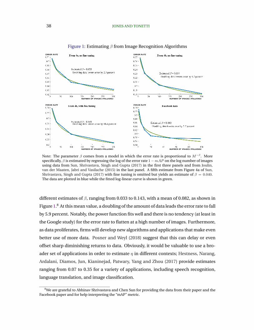
38 JONES AND TONETTI
Figure 1: Estimating β from Image Recognition Algorithms
Note: The parameter β comes from a model in which the error rate is proportional to M−β . Morespecifically, β is estimated by regressing the log of the error rate 1−mAP on the log number of imagesusing data from Sun, Shrivastava, Singh and Gupta (2017) in the first three panels and from Joulin,van der Maaten, Jabri and Vasilache (2015) in the last panel. A fifth estimate from Figure 4a of Sun,Shrivastava, Singh and Gupta (2017) with fine tuning is omitted but yields an estimate of β = 0.040.The data are plotted in blue while the fitted log-linear curve is shown in green.
different estimates of β, ranging from 0.033 to 0.143, with a mean of 0.082, as shown in
Figure 1.8 At this mean value, a doubling of the amount of data leads the error rate to fall
by 5.9 percent. Notably, the power function fits well and there is no tendency (at least in
the Google study) for the error rate to flatten at a high number of images. Furthermore,
as data proliferates, firms will develop new algorithms and applications that make even
better use of more data. Posner and Weyl (2018) suggest that this can delay or even
offset sharp diminishing returns to data. Obviously, it would be valuable to use a bro-
ader set of applications in order to estimate η in different contexts; Hestness, Narang,
Ardalani, Diamos, Jun, Kianinejad, Patwary, Yang and Zhou (2017) provide estimates
ranging from 0.07 to 0.35 for a variety of applications, including speech recognition,
language translation, and image classification.
8We are grateful to Abhinav Shrivastava and Chen Sun for providing the data from their paper and theFacebook paper and for help interpreting the “mAP” metric.

NONRIVALRY AND THE ECONOMICS OF DATA 39
In order to map the estimate of β into the parameter η in our model, we need
to make some assumption about how the error rate translates into productivity. If
productivity equals the inverse of the error rate, then η = β. However, there is no
reason why this assumption needs to hold, and one could imagine that productivity is
the error rate raised to some other exponent. Without knowledge of this exponent, we
cannot map the estimates from the machine learning literature directly into η. Hence,
we prefer our earlier approach to calibration based on data’s share of GDP. What we find
most valuable about the machine learning evidence is that it supports the power law
formulation that is assumed in our model.
Other parameters. Other parameter values used in our example are reported in Ta-
ble 2. We consider an elasticity of substitution of 4 implying that the degree of incre-
asing returns in the economy is 1σ−1 = 0.33 when there are no data sales, rising to
1σ−1 + η
1−η = 0.40 when data is used broadly; our baseline value of η = 0.06 implies η/(1−
η) = 0.064. Population growth in advanced economies is around 1 percent per year,
but the growth rate of R&D labor is closer to 4 percent; as a compromise, we choose
gL = 0.02. Combined with the returns to scale, this implies steady-state growth rates of
consumption per person of 0.67 percent when selling data is outlawed and 0.79 percent
when data is used broadly. Of course these are lower than what we see in advanced
economies, but our model omits quality improvements within firms/varieties, so we
probably should not match a higher growth rate. We set L0 = 100, corresponding to a
workforce of around 100 million people; labor units are therefore millions of people. We
set the rate of time preference to 2.5 percent (it must be larger than gL). Entry requires
χ = 0.01 workers; because labor units are in millions of people, this corresponds to
10,000 people, and with an R&D share of the population of around 1 percent, this would
mean 100 researchers. We set the weight on own data to α = 0.5; this parameter plays
very little role in our results.
The privacy and creative destruction parameters and less standard, so we choose
baseline values, but also explore a wide range of values in our numerical exercise. Re-
garding the privacy cost parameters, κ and κ, Athey, Catalini and Tucker (2017) show
that people express concerns about privacy but are willing to share once incentivized,
even by a relatively small reward: a majority of MIT students in their survey were wil-
40 JONES AND TONETTI
Table 2: Parameter Values
Description Parameter Value
Importance of data η 0.06
Elasticity of substitution (goods) σ 4
Weight on privacy κ = κ 0.20
Population level L0 100
Population growth rate gL 0.02
Rate of time preference ρ 0.025
Labor cost of entry χ 0.01
Creative destruction δ0 0.4
Weight on own data α 1/2
Elasticity of substitution (data) ε 50
Use of own data in OS x 1
Note: Baseline parameter values for the numerical example.
ling to share the email addresses of three close friends in exchange for a free pizza.
Nevertheless, we give an important role to privacy; an individual’s privacy concerns
regarding all their economic activity may be different than that exhibited in the lab. We
set κ = 0.20, implying that having all of one’s data shared with all firms is equivalent
to a reduction in consumption of 10 percent; we explore robustness to values between
0.02 and 0.99. Selling all of a variety’s data increases the rate of creative destruction by
δ0/2, which we calibrate to 20 percent; absent any other death, this corresponds to an
expected lifetime of 5 years. We explore robustness to values of δ0 between 0.02 and
0.99.
9.1 Consumption-Equivalent Welfare
Consumers care about consumption as well as privacy. A consumption-equivalent
welfare measure incorporates both. Along a balanced growth path, welfare is given by
Uallocss =L0
ρ
(log calloc0 − κ
2x2alloc +
gallocc
ρ
).
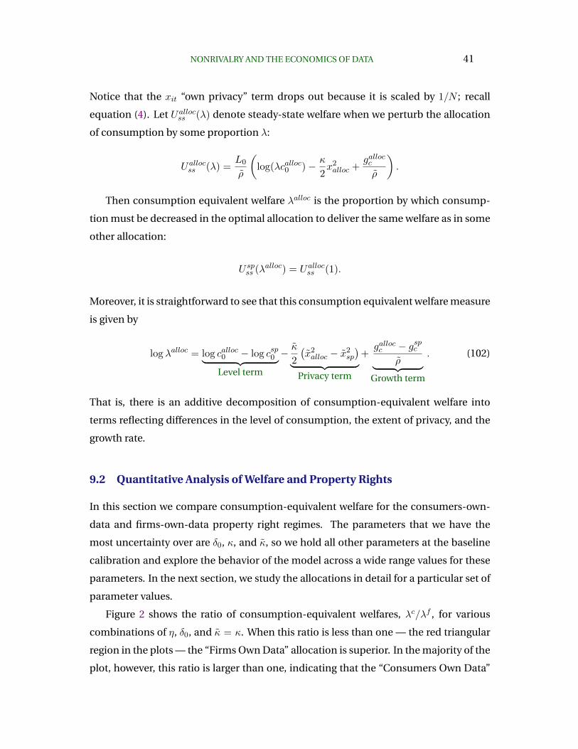
NONRIVALRY AND THE ECONOMICS OF DATA 41
Notice that the xit “own privacy” term drops out because it is scaled by 1/N ; recall
equation (4). Let Uallocss (λ) denote steady-state welfare when we perturb the allocation
of consumption by some proportion λ:
Uallocss (λ) =L0
ρ
(log(λcalloc0 )− κ
2x2alloc +
gallocc
ρ
).
Then consumption equivalent welfare λalloc is the proportion by which consump-
tion must be decreased in the optimal allocation to deliver the same welfare as in some
other allocation:
U spss (λalloc) = Uallocss (1).
Moreover, it is straightforward to see that this consumption equivalent welfare measure
is given by
log λalloc = log calloc0 − log csp0︸ ︷︷ ︸Level term
− κ2
(x2alloc − x2
sp
)︸ ︷︷ ︸
Privacy term
+gallocc − gspc
ρ︸ ︷︷ ︸Growth term
. (102)
That is, there is an additive decomposition of consumption-equivalent welfare into
terms reflecting differences in the level of consumption, the extent of privacy, and the
growth rate.
9.2 Quantitative Analysis of Welfare and Property Rights
In this section we compare consumption-equivalent welfare for the consumers-own-
data and firms-own-data property right regimes. The parameters that we have the
most uncertainty over are δ0, κ, and κ, so we hold all other parameters at the baseline
calibration and explore the behavior of the model across a wide range values for these
parameters. In the next section, we study the allocations in detail for a particular set of
parameter values.
Figure 2 shows the ratio of consumption-equivalent welfares, λc/λf , for various
combinations of η, δ0, and κ = κ. When this ratio is less than one — the red triangular
region in the plots — the “Firms Own Data” allocation is superior. In the majority of the
plot, however, this ratio is larger than one, indicating that the “Consumers Own Data”
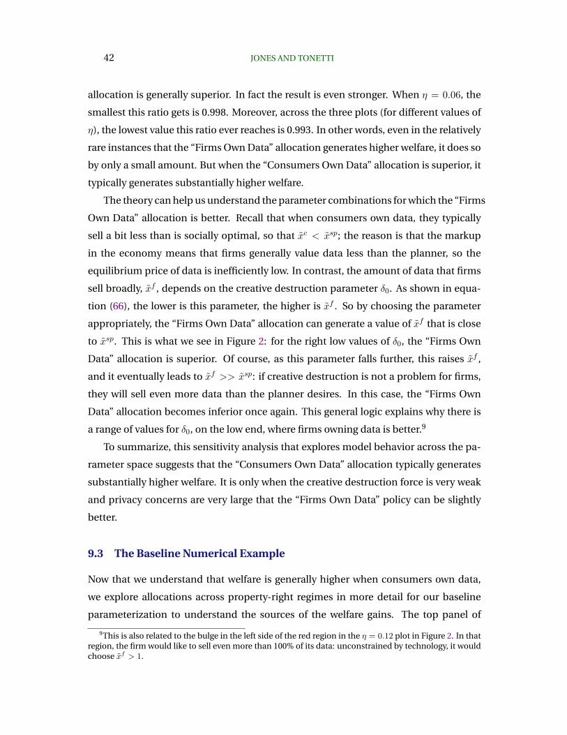
42 JONES AND TONETTI
allocation is generally superior. In fact the result is even stronger. When η = 0.06, the
smallest this ratio gets is 0.998. Moreover, across the three plots (for different values of
η), the lowest value this ratio ever reaches is 0.993. In other words, even in the relatively
rare instances that the “Firms Own Data” allocation generates higher welfare, it does so
by only a small amount. But when the “Consumers Own Data” allocation is superior, it
typically generates substantially higher welfare.
The theory can help us understand the parameter combinations for which the “Firms
Own Data” allocation is better. Recall that when consumers own data, they typically
sell a bit less than is socially optimal, so that xc < xsp; the reason is that the markup
in the economy means that firms generally value data less than the planner, so the
equilibrium price of data is inefficiently low. In contrast, the amount of data that firms
sell broadly, xf , depends on the creative destruction parameter δ0. As shown in equa-
tion (66), the lower is this parameter, the higher is xf . So by choosing the parameter
appropriately, the “Firms Own Data” allocation can generate a value of xf that is close
to xsp. This is what we see in Figure 2: for the right low values of δ0, the “Firms Own
Data” allocation is superior. Of course, as this parameter falls further, this raises xf ,
and it eventually leads to xf >> xsp: if creative destruction is not a problem for firms,
they will sell even more data than the planner desires. In this case, the “Firms Own
Data” allocation becomes inferior once again. This general logic explains why there is
a range of values for δ0, on the low end, where firms owning data is better.9
To summarize, this sensitivity analysis that explores model behavior across the pa-
rameter space suggests that the “Consumers Own Data” allocation typically generates
substantially higher welfare. It is only when the creative destruction force is very weak
and privacy concerns are very large that the “Firms Own Data” policy can be slightly
better.
9.3 The Baseline Numerical Example
Now that we understand that welfare is generally higher when consumers own data,
we explore allocations across property-right regimes in more detail for our baseline
parameterization to understand the sources of the welfare gains. The top panel of
9This is also related to the bulge in the left side of the red region in the η = 0.12 plot in Figure 2. In thatregion, the firm would like to sell even more than 100% of its data: unconstrained by technology, it wouldchoose xf > 1.
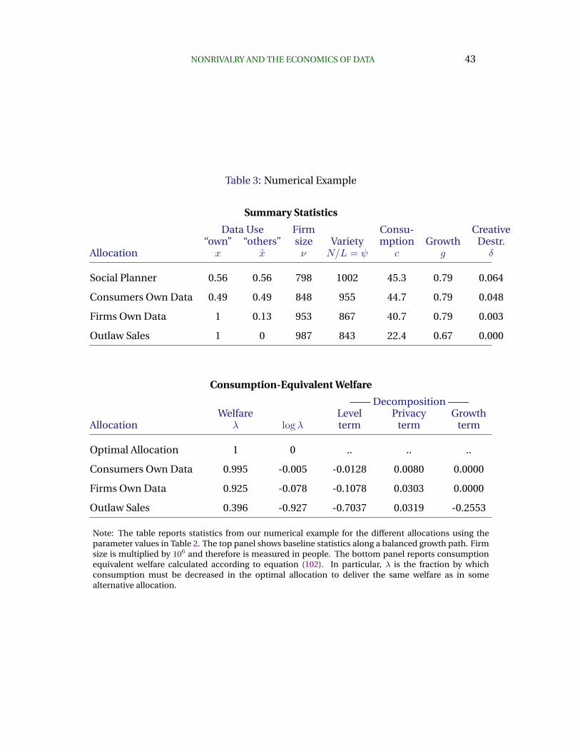
NONRIVALRY AND THE ECONOMICS OF DATA 43
Table 3: Numerical Example
Summary Statistics
Data Use Firm Consu- Creative“own” “others” size Variety mption Growth Destr.
Allocation x x ν N/L = ψ c g δ
Social Planner 0.56 0.56 798 1002 45.3 0.79 0.064
Consumers Own Data 0.49 0.49 848 955 44.7 0.79 0.048
Firms Own Data 1 0.13 953 867 40.7 0.79 0.003
Outlaw Sales 1 0 987 843 22.4 0.67 0.000
Consumption-Equivalent Welfare
—— Decomposition ——Welfare Level Privacy Growth
Allocation λ log λ term term term
Optimal Allocation 1 0 .. .. ..
Consumers Own Data 0.995 -0.005 -0.0128 0.0080 0.0000
Firms Own Data 0.925 -0.078 -0.1078 0.0303 0.0000
Outlaw Sales 0.396 -0.927 -0.7037 0.0319 -0.2553
Note: The table reports statistics from our numerical example for the different allocations using theparameter values in Table 2. The top panel shows baseline statistics along a balanced growth path. Firmsize is multiplied by 106 and therefore is measured in people. The bottom panel reports consumptionequivalent welfare calculated according to equation (102). In particular, λ is the fraction by whichconsumption must be decreased in the optimal allocation to deliver the same welfare as in somealternative allocation.
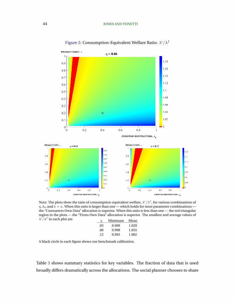
44 JONES AND TONETTI
Figure 2: Consumption-Equivalent Welfare Ratio: λc/λf
Note: The plots show the ratio of consumption-equivalent welfare, λc/λf , for various combinations ofη, δ0, and κ = κ. When this ratio is larger than one — which holds for most parameter combinations —the “Consumers Own Data” allocation is superior. When this ratio is less than one — the red triangularregion in the plots — the “Firms Own Data” allocation is superior. The smallest and average values ofλc/λf in each plot are η Minimum Mean
.03 0.999 1.029
.06 0.998 1.055
.12 0.993 1.082
A black circle in each figure shows our benchmark calibration.
Table 3 shows summary statistics for key variables. The fraction of data that is used
broadly differs dramatically across the allocations. The social planner chooses to share
NONRIVALRY AND THE ECONOMICS OF DATA 45
56 percent of data, even taking privacy considerations into account. When consumers
own data, they sell less at 49 percent.10 As discussed earlier, the reason for this dif-
ference is the monopoly markup σσ−1 = 1.33 that leads the price at which consumers
sell their data to be too low relative to what the planner would want. These “high use”
allocations can be contrasted with the bottom two allocations. When firms own data,
they distort the use of data in two ways. First, they use 100 percent of their own data,
more than what consumers or the planner would desire. In this sense, firms do not
satisfy the privacy concerns of consumers. Second, there is too little sharing with other
firms relative to the planner: firms sell only 13 percent of their data to other firms. The
key factor in this decision is creative destruction. And of course, when selling data is
outlawed, the allocation features no data sales.
The next two columns of the top panel show that firm size and the number of varie-
ties differ across the allocations. When firms own data or when selling is outlawed, the
rate of creative destruction is low (see the last column). Less creative destruction has
two countervailing effects. On the one hand, it raises the present value of profits, which
tends to promote entry. On the other hand, it reduces the boost to entry associated with
business stealing. When ρ > gL the business stealing effect dominates and higher rates
of creative destruction lead to more entry and smaller firms. This can be seen in the
top panel of Table 3, where the number of varieties is higher when consumers own data
than in the two limited-sales allocations. Similarly, firm size is smaller when consumers
own data.
The outlaw-sales equilibrium features a smaller scale effect, which shows up both
in economic growth being slower and in the overall level of consumption being sub-
stantially lower.
The bottom panel of Table 3 shows the welfare decomposition using the baseline
parameter values. The allocation in which data selling is outlawed is stunningly infe-
rior: consumption-equivalent welfare is only 40 percent of that of the social planner.
A small part of this is the growth rate differential, but the bulk comes from distortions
to the level of consumption, most importantly the missing scale effect associated with
broad data use. Laws that prohibit data sales can have dramatic effects, reducing inco-
mes substantially.
10In the planner and consumers-own-data allocations x = x because we’ve set κ = κ and α = 1/2.
46 JONES AND TONETTI
One institution that appropriately balances these concerns is assigning ownership
of data to consumers. Data use is close to that of the social planner and consumption-
equivalent welfare falls just short of optimal in this example. Consumers take their own
privacy considerations into account but are incentivized by markets to sell their data
broadly to a range of firms, leading them to nearly-optimal allocations.
In contrast, when firms own data, concerns about creative destruction sharply limit
the amount of data they sell to other firms. While limited sharing generates some
privacy benefits, equal to about 3 percent of consumption, the social loss from nonrival
data not being used by other firms is much larger. Of course, the way we’ve modeled
privacy is ad hoc, as privacy considerations are not the main focus of the paper. Ho-
wever, our baseline parameterization of κ was intentionally set to deliver large utility
costs from lack of privacy, and still the welfare losses are dominated by the use of data
in production.
Equilibrium welfare is just 93% of optimal when firms own data, compared to 99+%
of optimal when consumers own data. Failing to appropriately take advantage of the
nonrivalry of data leads consumption to be lower by more than seven percent along
the balanced growth path, even in this example in which there are sharply diminishing
returns to additional data.
10 Discussion
Implications for IO. Several issues related to antitrust and IO are raised by this fra-
mework. First, because firms see increasing returns to scale associated with data and,
perhaps more importantly, because of the nonrivalry of data, firms in this economy
would like to merge into a single economy-wide firm. Our paper provides a concept
of a firm as the boundary of data usage and the nonrivalry of data may create strong
pressures to increase scale. Return to the example of medical data being used within
hospital networks to improve the accuracy of diagnoses. If hospitals merged, they
would be able to estimate a more accurate algorithm, leading to better service on this
dimension for all of its patients.
Second, data may serve as a barrier to entry. A natural concern about the limited-
sales allocations is that as a firm accumulates data, this may make it harder for other
NONRIVALRY AND THE ECONOMICS OF DATA 47
firms to enter. In our framework, this force appears somewhat mechanically through
the dependence of the rate of creative destruction δ(x) on the amount of data sold. It
would be interesting in future research to consider this force more explicitly, say, in a
quality ladder model.
The Boundaries of Data Diffusion: Firms and Countries. At the beginning of the
paper, we noted that both ideas and data are nonrival. Both can be expressed as bit
strings, and it is natural to wonder about the differences between them. For example,
while ideas give rise to increasing returns and people create ideas, growth theory does
not typically suggest that Luxembourg and Hong Kong should be much poorer than
Germany and China because of their relatively small size. Instead, the view is that ideas
diffuse across countries, at least eventually and in general, so that the relevant scale is
the scale of the global market of connected countries rather than that of any individual
economy.
Data may be different. For example, it seems much easier to monitor and limit the
spread of data than to limit the spread of ideas. Perhaps this is because ideas, in order
to be useful, need to be embodied inside people in the form of human capital (which
makes it inherently hard to keep it from spreading). In contrast, data can be encrypted
and tightly controlled.
This raises an interesting question about whether the quantity of data that an or-
ganization has access to can serve as an important productivity advantage. This could
apply to firms or even to countries. For example, the Chinese economy is large. Could
access to the inherently larger quantities of data associated with a large population
provide an advantage. Lee (2018) suggests “China has more data than the US — way
more. Data is what makes AI go. A very good scientist with a ton of data will beat a
super scientist with a modest amount of data.” Similarly, a government that places a
lower weight on consumer privacy might induce more data sales, leading to a higher
level of aggregate output (but perhaps lower welfare). State-owned enterprises could
be encouraged to share data with each other. Or, in an industry context with trade, this
difference could lead to firms (e.g., in China) having a distinct productivity advantage
in data-intensive products.
48 JONES AND TONETTI
11 Conclusion
The economics of data raises many important questions. Privacy concerns have appro-
priately received a great deal of attention recently. Our framework supports this: when
firms own data, they may overuse it and not adequately respect consumer privacy.
But another important consideration arises from the nonrivalry of data. Because
data is infinitely usable, there are large social gains to allocations in which the same
data is used by multiple firms simultaneously. Consider our own profession. There
are clearly substantial benefits in having data from the PSID, the CPS, and the National
Income and Product Accounts available for all to use. At the heart of these gains is
the fact that data is nonrival. It is technologically feasible for medical data to be widely
used by health researchers and for all driving data to be used by every machine learning
algorithm. Yet when firms own such data, they may be reluctant to sell it because of
concerns over creative destruction. Our numerical examples suggest that the welfare
costs arising from limits to using nonrival data can be large.
Government restrictions that, out of a concern for privacy, outlaw selling data enti-
rely may be particularly harmful. Instead, our analysis indicates that giving data pro-
perty rights to consumers can lead to allocations that are close to optimal. Consumers
balance their concerns for privacy against the economic gains that come from selling
data to all interested parties.
NONRIVALRY AND THE ECONOMICS OF DATA 49
References
Abowd, John M. and Ian M. Schmutte, “An Economic Analysis of Privacy Protection and
Statistical Accuracy as Social Choices,” American Economic Review, 2019, 2019 (1), 171–202.
Acquisti, Alessandro, Curtis Taylor, and Liad Wagman, “The Economics of Privacy,” Journal of
Economic Literature, June 2016, 54 (2), 442–92.
Aghion, Philippe and Peter Howitt, “A Model of Growth through Creative Destruction,” Econo-
metrica, March 1992, 60 (2), 323–351.
Agrawal, Ajay, Joshua Gans, and Avi Goldfarb, Prediction Machines: The simple economics of
artificial intelligence, Harvard Business Press, 2018.
Akcigit, Ufuk and Qingmin Liu, “The Role of Information in Innovation and Competition,”
Journal of the European Economic Association, 2016, 14 (4), 828–870.
, Murat Alp Celik, and Jeremy Greenwood, “Buy, Keep, or Sell: Economic Growth and the
Market for Ideas,” Econometrica, 2016, 84 (3), 943–984.
Ali, S. Nageeb, Ayal Chen-Zion, and Erik Lillethun, “Reselling Information,” working paper,
2019.
, Greg Lewis, and Shoshana Vasserman, “Voluntary Disclosure and Personalized Pricing,”
working paper, 2018.
Arrieta Ibarra, Imanol, Leonard Goff, Diego Jimenez Hernandez, Jaron Lanier, and E. Glen Weyl,
“Should We Treat Data as Labor? Moving Beyond ”Free”,” American Economic Association
Papers and Proceedings, 2018, pp. 38–42.
Athey, Susan, Christian Catalini, and Catherine Tucker, “The Digital Privacy Paradox: Small
Money, Small Costs, Small Talk,” Working Paper 23488, National Bureau of Economic
Research June 2017.
Azevedo, Eduardo M., Alex Deng, Jose Montiel Olea, Justin M Rao, and E Glen Weyl, “A/B Testing
with Fat Tails,” 2019. University of Pennsylvania manuscript.
Bajari, Patrick, Victor Chernozhukov, Ali Hortacsu, and Junichi Suzuki, “The Impact of Big Data
on Firm Performance: An Empirical Investigation,” Working Paper 24334, National Bureau of
Economic Research February 2018.
Begenau, Juliane, Maryam Farboodi, and Laura Veldkamp, “Big Data in Finance and the Growth
of Large Firms,” 2017. NYU manuscript.
50 JONES AND TONETTI
Benassy, Jean-Pascal, “Taste for Variety and Optimum Production Patterns in Monopolistic
Competition,” Economics Letters, 1996, 52 (1), 41–47.
Bergemann, Dirk and Alessandro Bonatti, “Markets for Information: An Introduction,” Annual
Review of Economics, 2019, 11 (1), null.
Bollard, Albert, Peter J. Klenow, and Huiyu Li, “Entry Costs Rise with Development,” 2016.
Stanford University manuscript.
Carriere-Swallow, Yan and Vikram Haksar, “The Economics and Implications of Data: An
Integrated Perspective,” June 2019. IMF unpublished manuscript.
Chari, V. V. and Larry E. Jones, “A Reconsideration of the Problem of Social Cost: Free Riders and
Monopolists,” Economic Theory, 2000, 16 (1), 1–22.
Chiou, Lesley and Catherine Tucker, “Search Engines and Data Retention: Implications for Pri-
vacy and Antitrust,” Working Paper 23815, National Bureau of Economic Research September
2017.
Coase, Ronald H., “The Problem of Social Cost,” The Journal of Law and Economics, 1960, 3,
1–44.
Dixit, Avinash K. and Joseph E. Stiglitz, “Monopolistic Competition and Optimum Product
Diversity,” American Economic Review, June 1977, 67, 297–308.
Dosis, Anastasios and Wilfried Sand-Zantman, “The Ownership of Data,” July 2019. University
of Toulouse, unpublished manuscript.
Fajgelbaum, Pablo D., Edouard Schaal, and Mathieu Taschereau-Dumouchel, “Uncertainty
Traps,” The Quarterly Journal of Economics, 2017, 132 (4), 1641–1692.
Farboodi, Maryam and Laura Veldkamp, “Long Run Growth of Financial Technology,” NBER
Working Papers 23457, National Bureau of Economic Research, Inc May 2017.
and , “A Growth Model of the Data Economy,” working paper, 2019.
Goldfarb, Avi and Catherine E. Tucker, “Privacy Regulation and Online Advertising,” Manage-
ment science, 2011, 57 (1), 57–71.
Hestness, Joel, Sharan Narang, Newsha Ardalani, Gregory F. Diamos, Heewoo Jun, Hassan
Kianinejad, Md. Mostofa Ali Patwary, Yang Yang, and Yanqi Zhou, “Deep Learning Scaling
is Predictable, Empirically,” CoRR, 2017, abs/1712.00409.

NONRIVALRY AND THE ECONOMICS OF DATA 51
Hughes-Cromwick, Ellen and Julia Coronado, “The Value of US Government Data to US
Business Decisions,” Journal of Economic Perspectives, February 2019, 33 (1), 131–46.
Ichihashi, Shota, “Non-Competing Data Intermediaries,” June 2019. Bank of Canada, unpublis-
hed manuscript.
Joulin, Armand, Laurens van der Maaten, Allan Jabri, and Nicolas Vasilache, “Learning Visual
Features from Large Weakly Supervised Data,” CoRR, 2015, abs/1511.02251.
Lee, Kai-Fu, “Tech companies should stop pretending AI won’t destroy jobs,” MIT Technology
Review, February 21 2018.
Miller, Amalia R. and Catherine Tucker, “Privacy Protection, Personalized Medicine, and
Genetic Testing,” Management Science, 2017, 64 (10), 4648–4668.
Ordonez, Guillermo, “The Asymmetric Effects of Financial Frictions,” Journal of Political
Economy, 2013, 121 (5), 844–895.
Posner, Eric A. and E. Glen Weyl, Radical Markets: Uprooting Capitalism and Democracy for a
Just Society, Princeton University Press, 2018.
Romer, Paul M., “Endogenous Technological Change,” Journal of Political Economy, October
1990, 98 (5), S71–S102.
Sun, Chen, Abhinav Shrivastava, Saurabh Singh, and Abhinav Gupta, “Revisiting Unreasonable
Effectiveness of Data in Deep Learning Era,” CoRR, 2017, abs/1707.02968.
Varian, Hal, “Artificial Intelligence, Economics, and Industrial Organization,” in Ajay K. Agrawal,
Joshua Gans, and Avi Goldfarb, eds., The Economics of Artificial Intelligence: An Agenda,
University of Chicago Press, 2018.
Veldkamp, Laura, “Slow Boom, Sudden Crash,” Journal of Economic Theory, 2005, 124 (2), 230–
257.